SOCSol4L

AN IMPROVED MATLAB R© PACKAGE FOR APPROXIMATING THESOLUTION TO A CONTINUOUS-TIME STOCHASTIC OPTIMAL CONTROL

PROBLEM

JEFFREY D. AZZATO & JACEK B. KRAWCZYK

Abstract. Computing the solution to a stochastic optimal con-trol problem is difficult. A method of approximating a solu-tion to a given continuous-time stochastic optimal controlproblem using Markov chains was developed in [Kra01].This paper describes a suite of MATLAB R© routines imple-menting this method.

2006 Working PaperSchool of Economics and Finance

JEL Classification: C63 (Computational Techniques), C87 (Economic Software).AMS Categories: 93E25 (Computational methods in stochastic optimal control).

Authors’ Keywords: Computational economics, Approximating Markov decision chains.

This report documents 2005–2007 research intoComputational Economics Methodsdirected by Jacek B. Krawczyk and

supported by VUW FCA FRG-05 (24644)

Correspondence should be addressed to:

Jacek B. Krawczyk. Faculty of Commerce and Administration, Victoria University of Wellington,

P.O. Box 600, Wellington, New Zealand. Fax: +64-4-4635014 Email:

J.Krawczykatvuw.ac.nz Webpage: http://www.vuw.ac.nz/staff/jacek_krawczyk

Contents

Introduction 1

1. SOCSol 2

1.1. Purpose 2

1.2. Syntax 2

2. ContRule 7

2.1. Purpose 7

2.2. Syntax 7

3. GenSim 8

3.1. Purpose 8

3.2. Implementation 8

3.3. Syntax 8

4. ValGraph 10

4.1. Purpose 10

4.2. Syntax 10

5. LagranMap 11

5.1. Purpose 11

5.2. Syntax 11

6. Technical Information 13

6.1. Encoding the State Space 13

6.2. The Solution Files 14

7. Hints 15

7.1. Choosing State Variable Bounds 15

7.2. Choosing Discretisation Step Sizes 15

7.3. Use of TolFun 16

7.4. Relative Magnitudes of Controls 16

7.5. Enforcing Bounds on Directly Controlled State Variables 16

7.6. Enforcing Bounds on Monotonic State Variables 17

7.7. Enforcing Terminal State Constraints 17

7.8. Retrieving Additional Information 17

Appendix A. Example of use of SOCSol4L 19

A.1. Optimisation Problem 19

A.2. Solution Syntax 20

A.3. Retrieving Results Syntax 21

References 24

Introduction

Computing the solution to a stochastic optimal control problem is difficult. A methodof approximating a solution to a given continuous-time stochastic optimal control(soc) problem using Markov chains was developed in [KW97] and subsequently im-

proved in [Kra01]. This paper describes a suite of MATLAB R©1 routines implementingthis method.

The suite of routines developed updates and extends that described in [AK06]. Fur-ther details on the underlying method are available in [Kra05]. In Appendix A weprovide an example showing how to generate a test result from [KW97].

The method deals with finite-horizon, free terminal state soc problems having theform

minu

J(u, x0) = E

[

∫ T

0f(

x(t), u(t), t)

dt + h(

x(T))

∣

∣

∣

∣

x(0) = x0

]

(1)

subject to

dx = g(

x(t), u(t), t)

dt + b(

x(t), u(t), t)

dW(2)

where W is a standard Wiener process. In the optimisation method, we also allow forconstraints on the control and state variables (local and mixed).

Note: Throughout the paper, the dimension of the state space shall be denoted by d,the dimension of the control by c, the length of the horizon by T, and the number ofvariables which are affected by noise by N (N 6 d).

To solve (1) subject to (2) and local constraints, we developed a package of MATLAB R©

programmes under the name SOCSol4L. The package is composed of five main mod-ules:

1. SOCSol2. ContRule3. GenSim4. ValGraph5. LagranMap

SOCSol discretises a given soc problem and then solves this “discretisation.” If theproblem is constrained, it can also produce maps from states and times to Lagrangemultipliers’ values. ContRule derives graphs of continuous-time, continuous-statecontrol rules from the SOCSol solution. GenSim simulates the continuous system usingsuch a control rule (also derived from the SOCSol solution). ValGraph provides anautomated means of computing expected values for the continuous system as initialconditions change. LagranMap produces graphs of Lagrange multipliers’ values fromLagrange maps generated by SOCSol.

1See [Mat92] for an introduction to MATLAB R©.

1

1. SOCSol

1.1. Purpose. SOCSol takes the given soc problem and approximates it with a Markovchain, which it then solves. This results in a discrete-time, discrete-space control rule.SOCSol does not perform the interpolation necessary to convert this discrete-time,discrete-space control rule into a continuous-time, continuous-state control rule (thisis done by GenSim).

1.2. Syntax. SOCSol is called as follows.

SOCSol ( ‘ Del taFunct ionFi le ’ , ‘ Ins tantaneousCostFunct ionFi le ’ ,‘ Termina lS ta teFunct ionFi le ’ , StateLB , StateUB , Sta teStep ,TimeStep , ‘ ProblemFile ’ , Options , I n i t i a l C o n t r o l V a l u e , A,b , Aeq , beq , ControlLB , ControlUB ,‘ UserConstra intFunct ionFi le ’ )

Note: It is easiest to define these arguments in a script, and then call that script inMATLAB R©. See Appendix A for an example of this.

DeltaFunctionFile:

A string giving the name (no .m extension) of a file containing a MATLAB R© functionrepresenting the equations of motion.

If the problem is deterministic, the function returns a vector of length d correspondingto the value of g

(

x(t), u(t), t)

.

If the problem is stochastic then the function returns a vector of length 2d, the firstd elements of which are g

(

x(t), u(t), t)

and the second d elements of which are

b(

x(t), u(t), t)

. If some of the variables are undisturbed by noise (i.e., N < d), thenthe variables for which the diffusion term is constantly 0 must follow those that aredisturbed by noise.

In either case the function should have a header of the form

function Value = Delta ( Control , S t a t e V a r i a b l e s , Time )

where Control is a vector of length c, StateVariables is a vector of length d, andTime is a scalar.

InstantaneousCostFunctionFile:

A string giving the name (no .m extension) of a file containing a MATLAB R© function

representing the instantaneous cost function f(

x(t), u(t), t)

.2 The function shouldhave a header of the form

function Value = Cost ( Control , S t a t e V a r i a b l e s , Time )

2A maximisation problem can be converted into a minimisation problem by multiplying the per-formance criterion by −1. Consequently, if the soc problem to be solved involves maximisation, thenegative of its instantaneous cost should be specified in InstantaneousCostFunctionFile.

2

where Control is a vector of length c, StateVariables is a vector of length d, andTime is a scalar.

TerminalStateFunctionFile:

A string containing the name (no .m extension) of a file containing a MATLAB R©

function representing the terminal state function h(

x(T))

. This function should return

only the single real value given by h(

x(T))

(even if the function is identically zero).3

The function should have a header of the form

function Value = Term ( S t a t e V a r i a b l e s )

where StateVariables is a vector of length d.

StateLB, StateUB, and StateStep:

These determine the finite state grid for the Markov chain that we hope will approxi-mate the soc problem. Each may be given as a vector or as an array, independent ofthe type of the other two.

The value of StateLB is the least possible state, while the value of StateUB is the

maximum possible state.4

The value of StateStep determines the distances between points of the state grid. Ithas to be chosen so that its entry/entries corresponding to the i-th state variable ex-actly divides/divide the difference/differences between the corresponding entries ofStateLB and StateUB. Of course, step size need not be the same for all state variables.

Each of these values can be given in two different ways:

1. As a vector of length d (the dimension of the state space, where each value in thevector corresponds to one dimension) In this case, the same set of numbers willapply to every decision stage of the Markov chain.

2. As a matrix with S + 1 rows and d columns, where S is the number of decisionstages in the Markov chain as determined by TimeStep below. The i-th row is thenused to determine the state grid in the i-th stage.

TimeStep:

This determines the number of decision stages and their associated times.

TimeStep is a vector of step lengths that partition the interval [0, T]; i.e., their sumshould be T. The number of elements of TimeStep is the number of decision stages inthe Markov chain, which we denote by S.

3A maximisation problem can be converted into a minimisation problem by multiplying the per-formance criterion by −1. Consequently, if the soc problem to be solved involves maximisation, thenegative of its terminal state should be specified in TerminalStateFunctionFile.

4The solution is routinely disturbed close to the state boundaries StateLB and StateUB. Conse-quently, these should be chosen “generously.” Of course, larger state grids require greater computationtimes—see Section 7.1 for advice.

3

ProblemFile:

A string containing the name (with no extension) of the problem. This name is usedto store the solution on disk. SOCSol produces at least two files with this name: onewith the extension .DPP, which contains the parameters used to compute the Markovchain, and one with the extension .DPS, which contains the solution itself. If theLagrangeMaps option (described below) is set to ‘yes’, a third file with the extension.DPL is also produced. This contains the Lagrange multipliers.

The .DPP and .DPS files are used by GenSim to produce the continuous-time,continuous-state control rule. Note that the routines ContRule, GenSim and ValGraph

(see Sections 2, 3 and 4 respectively) require that the .DPP and .DPS files exist andremain unchanged, while the routine LagranMap (see Section 5) requires that the .DPP

and .DPL files exist and remain unchanged.

Options:

This vector (in fact, a cell array) of strings controls various internal settings that needonly be adjusted infrequently. Two types of options can be set using the Options vec-tor: options directly related to SOCSol4L, and options used by fmincon, a MATLAB R©

routine employed by SOCSol4L.

The user need only specify those options that are to be changed from their defaultvalues. If all options are to remain at their default values, then Options should bepassed as empty, i.e., as { }.

In order to alter an option from its default value, the option should be named (in astring) followed directly by the value to which it is to be set (in another string). Forexample, if it was desired to set the ControlDimension option to 2 and turn on theDisplay, then Options could be set as

Options = { ‘ ControlDimension ’ ‘2 ’ ‘ Display ’ ‘ on ’ } ;

Note that the number 2 is entered as the string ‘2’ . While it is important that anoption be followed directly by the value to which it is to be set, option-value pairs canbe given in any order. So it would be equally valid to set the above as

Options = { ‘ Display ’ ‘ on ’ ‘ ControlDimension ’ ‘2 ’} ;

The options related directly to SOCSol4L are:

1. ControlDimension. This contains the value c for your problem. It must be givenas a natural number (in a string). The default value is 1.

2. StochasticProblem. This should be set to ‘yes’ if your problem is stochastic. Thedefault value is ‘no’, i.e., the problem is assumed to be deterministic.

3. NoisyVars. This should be set to the number N (in a string) if N < d. The defaultvalue is d, i.e., all variables are assumed to be noisy. If the problem is deterministic,SOCSol ignores the value of NoisyVars.

4. LagrangeMaps. This specifies whether SOCSol should produce an output file con-taining the Lagrange multipliers associated with the problem’s constraints. If so,

4

LagrangeMaps should be set to ‘yes’. The default value is ‘no’. This option mustbe enabled if the user later wishes to utilise the LagranMap routine (see Section 5).

In general, fmincon can use either large-scale or medium-scale algorithms. Whilelarge-scale algorithms are more efficient for some problems, the use of such an al-gorithm requires differentiability of the function to be minimised. This is not gener-ally true of the cost-to-go functions that SOCSol4L passes to fmincon. Consequently,SOCSol4L employs only fmincon’s medium-scale algorithms.

As a result of this, those fmincon options specific to large-scale algorithms are notset through the Options vector, but instead passed their default values by SOCSol4L.However, the fmincon options specific to medium-scale algorithms may be set throughthe Options vector. These include:

1. Diagnostics. This controls whether fmincon prints diagnostic information aboutthe cost-to-go functions that it minimises. The default value is ‘off’, butDiagnostics may also be set to ‘on’.

2. Display. This controls fmincon’s display level. The default value is ‘off’ (no dis-play), but Display may also be set to ‘iter’ (display output for each of fmincon’siterations), ‘final’ (display final output for each call to fmincon) and ‘notify’ (displayoutput only if non-convergence is encountered).

3. MaxFunEvals. This sets fmincon’s maximum allowable number of function evalua-tions. The default value is 100c, but MaxFunEvals may be set to any natural number(in a string).

4. MaxIter. This sets fmincon’s maximum allowable number of iterations. The de-fault value is 400, but MaxIter may be set to any natural number (in a string).

5. MaxSQPIter. This sets fmincon’s maximum allowable number of sequential qua-dratic programming steps. The default value is ∞, but MaxSQPIter may be set toany natural number (in a string).

6. TolCon. This sets fmincon’s termination tolerance on constraint violation. Thedefault value is 10−6, but TolCon may be set to any positive real number (in astring).

7. TolFun. This sets fmincon’s termination tolerance on function evaluation. Thedefault value is 10−6, but TolFun may be set to any positive real number (in astring). See Section 7.3 for more on the use of TolFun.

8. TolX. This sets fmincon’s termination tolerance on optimal control evaluation. Thedefault value is 10−6, but TolX may be set to any positive real number (in a string).

If necessary, it is also possible to set:

11. DerivativeCheck. This controls whether fmincon compares user-supplied analyticderivatives (e.g., gradients or Jacobians) to finite differencing derivatives. The de-fault value is ‘off’, but DerivativeCheck may also be set to ‘on’.

12. DiffMaxChange. This sets fmincon’s maximum allowable change in variables forfinite difference derivatives. The default value is 0.1, but DiffMaxChange may be setto any positive real number (in a string).

13. DiffMinChange. This sets fmincon’s minimum allowable change in variables forfinite difference derivatives. The default value is 10−8, but DiffMaxChange may beset to any positive real number (in a string).

5

14. OutputFcn. A string containing the name (no .m extension) of a file containing aMATLAB R© function that is to be called by fmincon at each of its iterations. Such afunction is typically used to retrieve/display additional data from fmincon.

See Optimization Options :: Argument and Options Reference (Optimization Toolbox)in MATLAB R© help for more information on output functions.

For more information on fmincon, and fmincon options in particular, see fmincon ::Functions (Optimization Toolbox) and Optimization Options :: Argument and Options Ref-erence (Optimization Toolbox) in MATLAB R© help.

InitialControlValue:

In general, a vector of initial values for the control variables. This is used by SOCSol4L

as an approximate starting point in its search for an optimal discrete-state, discrete-time decision rule. Consequently, it may be chosen with some inaccuracy.

A and b:

These allow for the imposition of the linear inequality constraint(s) Au 6 b on thecontrol variable(s). In general, A is a matrix and b is a vector. If there are no linearinequality constraints on the control variable(s), both A and b should be passed asempty: [ ].

Aeq and beq:

These allow for the imposition of the linear equality constraint(s) Aeq · u = beq onthe control variable(s). In general, Aeq is a matrix and beq is a vector. If there areno linear equality constraints on the control variable(s), both Aeq and beq should bepassed as empty: [ ].

ControlLB and ControlUB:

In general, vectors of lower and upper bounds (respectively) on the control variables.If a control variable has no lower bound, the corresponding entry of ControlLB shouldbe set to −Inf. Similarly, if a control variable has no upper bound, the correspondingentry of ControlUB should be set to Inf.

UserConstraintFunctionFile:

A string containing the name (no .m extension) of a file containing a MATLAB R© func-tion representing problem constraints (in particular, non-linear problem constraints).

This function should return the value of inequality constraints as a vector Value1 andthe value of equality constraints as a vector Value2, where inequality constraints arewritten in the form k

(

u, x, t)

6 0 and equality constraints are written in the form

keq(

u, x, t)

= 0.

The function should have a header of the form

function [ Value1 , Value2 ] = Constra int ( Control ,S t a t e V a r i a b l e s , TimeStep )

6

where Control is a vector of length c, StateVariables is a vector of length d, andTimeStep is a scalar.

Note that the TimeStep argument makes the time step for the relevant Markov chaintime readily available for incorporation in constraints. It should not be confused withthe Time arguments of the other user-specified functions, which correspond to theMarkov chain times themselves.

In the absence of constraints requiring the use of UserConstraintFunctionFile,UserConstraintFunctionFile should be passed as empty: [ ].

See fmincon :: Functions (Optimization Toolbox) in MATLAB R© help for further infor-mation about solution starting points, A, b, Aeq, beq, bounds and the specificationof non-linear problem constraints. Some hints on enforcing problem constraints aregiven in Sections 7.5, 7.6 and 7.7.

2. ContRule

2.1. Purpose. ContRule produces graphs of the continuous-time, continuous-state

control rule derived from the solution computed by SOCSol.5 Each control rule graphis produced for a given time and holds all but one state variable constant.

2.2. Syntax. ContRule is called as follows.

ContRule ( ‘ ProblemFile ’ , Time , I n i t i a l C o n d i t i o n ,V a r i a b l e O f I n t e r e s t , LineSpec ) ;

ControlValues = ContRule ( · · · ) ;

Calling ContRule without any output arguments produces control rule profiles forthe given time and displays some technical information in the MATLAB R© commandwindow. However, ContRule may also be called with a single output argument. Inthis instance, ContRule also assigns the output argument the values of the controlrules in the form of an M × c array, where

M =StateUBVariableOfInterest − StateLBVariableOfInterest

StateStepVariableOfInterest

+ 1.

So the rows of this array correspond to points of the VariableOfInterest-th dimen-sion of the state grid, while its columns correspond to control dimensions.

ProblemFile:

A string containing the name (with no extension) of the problem. This name is usedto retrieve the solution produced by SOCSol from the disk. ContRule requires that the.DPP and .DPS files produced by SOCSol still exist and remain unchanged.

5Analogous graphs of the Lagrange multipliers associated with problem constraints can be obtainedvia LagranMap—see Section 5.

7

Time:

A scalar in the interval [0, T] telling ContRule the time for which a control profile is tobe computed. If Time is not a Markov chain time, ContRule computes a control profilefor the last Markov chain time before Time.

InitialCondition:

A vector determining the values of the fixed state variables. A value must be givenfor the VariableOfInterest as a placeholder, although this value is not used.

VariableOfInterest:

A scalar telling the routine which of the state variables to vary, i.e., numbers like “1”or “2” etc. have to be entered in accordance with the state variables’ ordering in thefunction DeltaFunctionFile. The control rule profile appears with the nominatedstate variable along the horizontal axis.

LineSpec:

This specifies the line style, marker symbol and colour of timepaths. It is a string ofthe format discussed in the LineSpec :: Functions (MATLAB Function Reference) sectionof MATLAB R© help.

If LineSpec is not specified, it defaults to ‘r-’ (a solid red line without markers).

3. GenSim

3.1. Purpose. GenSim takes the solution computed by SOCSol, derives a continuous-time, continuous-state control rule and simulates the continuous system using thisrule. It returns graphs of the timepaths of the state and control variables and theassociated performance criterion values for one or more simulations.

3.2. Implementation. The derivation of the continuous-time, continuous-state controlrule from the solution computed by SOCSol requires some form of interpolation inboth state and time. In an effort to keep the script simple the interpolation in stateis linear. States that are outside the state grid simply move to the nearest state gridpoint. For times between Markov chain times, the control profile for the most recentMarkov chain time is used.

The differential equation that governs the evolution of the system is simulated by in-terpolation of its Euler-Maruyama approximation. The performance criterion integralis approximated using the left-hand endpoint rectangle rule.

3.3. Syntax. GenSim is called as follows.

SimulatedValue = GenSim ( ‘ ProblemFile ’ , I n i t i a l C o n d i t i o n ,SimulationTimeStep , NumberOfSimulations , LineSpec ,TimepathOfInterest , UserSuppliedNoise )

8

ProblemFile:

A string containing the name (with no extension) of the problem. This name is usedto retrieve the solution produced by SOCSol from the disk. GenSim requires that the.DPP and .DPS files produced by SOCSol still exist and remain unchanged.

InitialCondition:

This is a vector of length d that contains the initial condition: the point from whichthe simulation starts.

SimulationTimeStep:

This is a vector of step lengths that partition interval [0, T]; i.e., their sum should beT.

With more simulation steps there is less error from approximating the equations ofmotion using the Euler-Maruyama scheme and from approximating the performancecriterion using the left-hand endpoint rectangle method. In general, the simulationstep is much smaller than the time step used to compute the solution (i.e., smallerthan the TimeStep argument given to SOCSol).

If no SimulationTimeStep vector is given, the SimulationTimeStep vector defaults tothe TimeStep vector used for computing the ProblemFile.

NumberOfSimulations:

This is the number of simulations that should be performed. If NumberOfSimulationsis passed as negative, GenSim performs |NumberOfSimulations| simulations, but doesnot plot any timepaths.

Multiple simulations are normally performed when dealing with a stochastic sys-tem. Each simulation uses a randomly determined noise realisation (unless this issuppressed by the UserSuppliedNoise argument).

If NumberOfSimulations is not specified, it defaults to 1.

LineSpec:

This specifies the line style, marker symbol and colour of timepaths. It is a string ofthe format discussed in the LineSpec :: Functions (MATLAB Function Reference) sectionof MATLAB R© help.

If LineSpec is not specified, it defaults to ‘r-’ (a solid red line without markers).

TimepathOfInterest:

This is an integer between 0 and d + c (inclusive) that specifies which timepath(s)GenSim is to plot. If TimepathOfInterest is passed the value 0, GenSim plots timepathsfor all state and control variables. Otherwise, if TimepathOfInterest is passed thevalue i > 0, GenSim plots the timepath of the i-th variable, where state variablesprecede control variables.

If TimepathOfInterest is not specified, it defaults to 0.

9

UserSuppliedNoise:

This entirely optional argument enables the user to override the random generationof noise realisations. If UserSuppliedNoise is passed the value 0, a constantly 0 noiserealisation is used. Otherwise, UserSuppliedNoise should be passed a matrix with Ncolumns and a row for each entry of SimulationTimeStep.

Note that NumberOfSimulations should be 1 if UserSuppliedNoise is specified. IfUserSuppliedNoise is left unspecified, GenSim randomly selects a standard Gaussiannoise realisation for each simulation. Naturally, UserSuppliedNoise has no effect ondeterministic problems.

SimulatedValue:

The MATLAB R© output consists of a vector of the values of the performance criterionfor each of the simulations performed.

If the problem is stochastic and noise realisations are random, then the average ofthe values from a large number of simulations can be used as an approximation tothe expected value of the continuous stochastic system (under the continuous-time,continuous-state control rule derived from the solution computed by SOCSol). Thisaverage is left for the user to compute.

4. ValGraph

4.1. Purpose. ValGraph automates the process of computing expected values for thecontinuous system (under the continuous-time, continuous-state control rule derivedfrom the solution computed by SOCSol) as the initial conditions change. In a similarspirit to ContRule (see Section 2), it deals with one state variable at a time (identifiedby VariableOfInterest), while the other state variables remain fixed.

4.2. Syntax. ValGraph is called as follows.

ValGraph ( ‘ ProblemFile ’ , I n i t i a l C o n d i t i o n , V a r i a b l e O f I n t e r e s t ,Var iab leOf Interes tVa lues , SimulationTimeStep ,NumberOfSimulations , Sca leFac tor , LineSpec )

ProblemFile:

A string containing the name (with no extension) of the problem. This name is usedto retrieve the solution produced by SOCSol from the disk. ValGraph requires that the.DPP and .DPS files produced by SOCSol still exist and remain unchanged.

InitialCondition:

A vector determining the values of the fixed state variables. A value must be givenfor the VariableOfInterest as a placeholder, although this value is not used.

10

VariableOfInterest:

A scalar telling the routine which of the state variables to vary. The value graphappears with this state variable along the horizontal axis.

VariableOfInterestValues:

A vector containing the values of the VariableOfInterest at which the system’s per-formance is to be evaluated.

SimulationTimeStep:

This is as for GenSim in Section 3.

NumberOfSimulations:

This is the number of simulations that should be performed. NumberOfSimulations

behaves like the identically-named argument for GenSim in Section 3, except if passedthe value 1 for a stochastic problem, it yields a constantly zero noise realisation.

If NumberOfSimulations is not specified, it defaults to 1.

ScaleFactor:

This simply scales all the resulting values by the given factor.

Maximisation problems must have all payoffs replaced by their negatives before entryinto SOCSol, as it assumes that problems require minimisation. Setting ScaleFactor

to −1 “corrects” the sign on payoffs for maximisation problems.

Naturally, if ScaleFactor is not specified, it defaults to 1.

LineSpec:

This specifies the line style, marker symbol and colour of timepaths. It is a string ofthe format discussed in the LineSpec :: Functions (MATLAB Function Reference) sectionof MATLAB R© help.

If LineSpec is not specified, it defaults to ‘r-’ (a solid red line without markers).

5. LagranMap

5.1. Purpose. LagranMap utilises SOCSol’s output to produce graphs of the Lagrange

multipliers associated with problem constraints.6 Each Lagrange map graph is pro-duced for a given time and holds all but one state variable constant.

5.2. Syntax. LagranMap is called as follows.

LagranMap ( ‘ ProblemFile ’ , Time , I n i t i a l C o n d i t i o n ,V a r i a b l e O f I n t e r e s t , LineSpec , M u l t i p l i e r O f I n t e r e s t ) ;

6Analogous graphs of the problem’s controls can be obtained via ContRule—see Section 2.

11

LagrangeValues = LagranMap ( · · · ) ;

Calling LagranMap without any output arguments produces Lagrange multiplier pro-files for the given time and displays some technical information in the MATLAB R©

command window. However, LagranMap may also be called with a single output ar-gument. In this instance, LagranMap also assigns the output argument the values ofthe Lagrange multipliers in the form of an M × c array, where

M =StateUBVariableOfInterest − StateLBVariableOfInterest

StateStepVariableOfInterest

+ 1.

So the rows of this array correspond to points of the VariableOfInterest-th dimen-sion of the state grid, while its columns correspond to control dimensions.

ProblemFile:

A string containing the name (with no extension) of the problem. This name is usedto retrieve the solution produced by SOCSol from the disk. LagranMap requires that

this solution include a .DPL file,7 and that the .DPP and .DPL files produced by SOCSol

still exist and remain unchanged.

Time:

A scalar in the interval [0, T] telling LagranMap the time for which Lagrange mapprofile is to be computed. If Time is not a Markov chain time, LagranMap computes aLagrange map profile for the last Markov chain time before Time.

InitialCondition:

A vector determining the values of the fixed state variables. A value must be givenfor the VariableOfInterest as a placeholder, although this value is not used.

VariableOfInterest:

A scalar telling the routine which of the state variables to vary, i.e., numbers like “1”or “2” etc. have to be entered in accordance with the state variables’ ordering in thefunction DeltaFunctionFile. The Lagrange map profile appears with the nominatedstate variable along the horizontal axis.

LineSpec:

This specifies the line style, marker symbol and colour of timepaths. It is a string ofthe format discussed in the LineSpec :: Functions (MATLAB Function Reference) sectionof MATLAB R© help.

If LineSpec is not specified, it defaults to ‘r-’ (a solid red line without markers).

MultplierOfInterest:

This is an integer between 0 and the number of bounds & constraints (inclusive) thatspecifies which Lagrange map(s) LagranMap is to plot. If MultplierOfInterest is

7See Options in Section 1.2.

12

passed the value 0, LagranMap plots Lagrange maps for all bounds and constraints.Otherwise, if MultplierOfInterest is passed the value i > 0, LagranMap plots theLagrange map of the i-th bound/constraint.

If MultplierOfInterest is not specified, it defaults to 0.

6. Technical Information

6.1. Encoding the State Space. Each point of the state grid is assigned a unique num-ber in the SOCSol routine. This state number is then used as an index in all theresultant matrices.

A CodingVector is computed for each stage. As a precursor to this, the number ofstates along each of the d state variable axes is first computed by

S t a t e s = round ( ( Max − Min ) . / S t a t e S t e p + 1 ) ;

where Max, Min, and StateStep are vectors appropriate for the current stage. Takingthe product of the entries of States gives TotalStates for the current stage. TheCodingVector is then defined by

c = cumprod ( S t a t e s ) ;CodingVector = [ 1 , c ( 1 : Dimension − 1 ) ] ;

where Dimension is the internal name for d, the number of state variables. TheCodingVector is used to compute the state number for each point of the state gridfor the current stage.

Suppose that x is a point of the state grid. Then x is converted into a vector ofnumbers called StateVector (which has 1 ≤ StateVector(i) ≤ States(i) for eachi = 1, . . . , d) by

S t a t e V e c t o r = round ( ( x − Min ) . / S t a t e S t e p + 1 ) ;

Finally, the state number for x, called State, is computed by taking the dot productof StateVector - 1 with the CodingVector and then adding 1, i.e.,

S t a t e = ( S t a t e V e c t o r − 1)∗ CodingVector + 1 ;

This process assigns a unique State to each point of the state grid. Every numberbetween 1 and TotalStates (inclusive) corresponds to a point of the state grid. Byconstruction, 1 corresponds to Min and TotalStates to Max.

Converting a state number back into a point of the state grid is equally simple. Thefirst step is to convert the State into a StateVector. This is carried out by a functionSnToSVec:

function S t a t e V e c t o r = SnToSVec ( StateNumber , CodingVector ,Dimension )

StateNumber = StateNumber − 1 ;S t a t e V e c t o r = zeros ( 1 , Dimension ) ;

13

for i = Dimension : −1:1S t a t e V e c t o r ( i ) = f l o o r ( StateNumber/CodingVector ( i ) ) ;StateNumber = StateNumber

− S t a t e V e c t o r ( i )∗ CodingVector ( i ) ;end ;

S t a t e V e c t o r = S t a t e V e c t o r + 1 ;

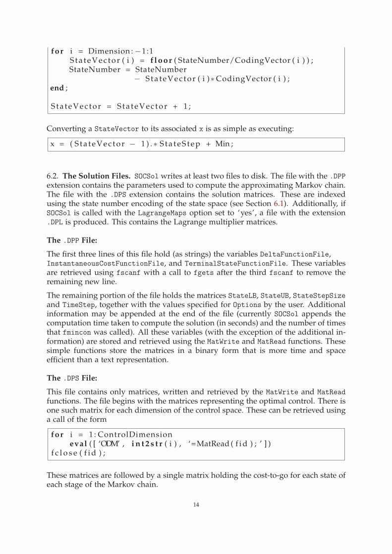
Converting a StateVector to its associated x is as simple as executing:

x = ( S t a t e V e c t o r − 1 ) . ∗ S t a t e S t e p + Min ;

6.2. The Solution Files. SOCSol writes at least two files to disk. The file with the .DPP

extension contains the parameters used to compute the approximating Markov chain.The file with the .DPS extension contains the solution matrices. These are indexedusing the state number encoding of the state space (see Section 6.1). Additionally, ifSOCSol is called with the LagrangeMaps option set to ‘yes’, a file with the extension.DPL is produced. This contains the Lagrange multiplier matrices.

The .DPP File:

The first three lines of this file hold (as strings) the variables DeltaFunctionFile,InstantaneousCostFunctionFile, and TerminalStateFunctionFile. These variablesare retrieved using fscanf with a call to fgets after the third fscanf to remove theremaining new line.

The remaining portion of the file holds the matrices StateLB, StateUB, StateStepSizeand TimeStep, together with the values specified for Options by the user. Additionalinformation may be appended at the end of the file (currently SOCSol appends thecomputation time taken to compute the solution (in seconds) and the number of timesthat fmincon was called). All these variables (with the exception of the additional in-formation) are stored and retrieved using the MatWrite and MatRead functions. Thesesimple functions store the matrices in a binary form that is more time and spaceefficient than a text representation.

The .DPS File:

This file contains only matrices, written and retrieved by the MatWrite and MatRead

functions. The file begins with the matrices representing the optimal control. There isone such matrix for each dimension of the control space. These can be retrieved usinga call of the form

for i = 1 : ControlDimensioneval ( [ ‘ODM’ , i n t 2 s t r ( i ) , ‘=MatRead ( f i d ) ; ’ ] )

f c l o s e ( f i d ) ;

These matrices are followed by a single matrix holding the cost-to-go for each state ofeach stage of the Markov chain.

14

The .DPL File:

This file also contains only matrices, written and retrieved by the MatWrite andMatRead functions. The file begins with six matrices (in fact, scalars) that respectivelygive the numbers of lower bounds, upper bounds, linear inequalities, linear equalities,non-linear inequalities and non-linear equalities that constrain the controls. These arethen followed by matrices representing each of these constraints, grouped in the orderabove. The matrices can be retrieved using a call of the form:

NumLower = MatRead ( f i d ) ;NumUpper = MatRead ( f i d ) ;NumIneqLin = MatRead ( f i d ) ;NumEqLin = MatRead ( f i d ) ;NumIneqNonlin = MatRead ( f i d ) ;NumEqNonlin = MatRead ( f i d ) ;for i = 1 :NumLower

eval ( [ ‘ LagrangeLower ’ , i n t 2 s t r ( i ) , ‘=MatRead ( f i d ) ; ’ ] ) ;end ;f o r j = 1 :NumUpper

eval ( [ ‘ LagrangeUpper ’ , i n t 2 s t r ( j ) , ‘=MatRead ( f i d ) ; ’ ] ) ;end ;...

7. Hints

7.1. Choosing State Variable Bounds. The formulation of a soc problem may giverise to a “natural” choice of bounds on its state variable(s), e.g., x1 ∈ [0, 0.5]. However,SOCSol4L’s solutions are routinely disturbed close to the bounds specified. Conse-quently, it may be sensible to specify a larger state grid than might initially appearnecessary (e.g., x1 ∈ [−0.2, 0.7]). Figure 1 demonstrates how this can move distortionoutside the area of interest.

Of course, ceteris paribus, specifying a larger state grid increases computation time. Ifthe soc problem has many dimensions, this increase may be considerable.

7.2. Choosing Discretisation Step Sizes. The choice of state step(s) and the choice oftime step are not entirely independent. In particular, the time step should not be “toosmall” in comparison to the state step(s). This is because some control u is optimalfor the Markov chain at a given grid point. However, the control chosen at this pointis a multiple of the time step. So if the time step is “too small,” u cannot be realised,

making the optimal solution unobtainable.8

Empirical evidence suggests that the time step can also be “too large” in comparisonto the state step(s). It is thus desirable to try a variety of discretisations, which maythen indicate some choices of step sizes that are effective for a particular problem.This is easily done by extending the script suggested in Section 1.2 to call SOCSol

several times, specifying ProblemFile differently each time.

8See p. 16 of [Kra01] for further discussion.

15

−0.2 −0.1 0 0.1 0.2 0.3 0.4 0.5 0.6 0.7−1

−0.8

−0.6

−0.4

−0.2

0

0.2

Con

trol

State

Figure 1. Control rules with distortion at the right.

7.3. Use of TolFun. When fine discretisation is used (in particular, a small time step),the cost-to-go functions that fmincon must minimise are relatively flat. Consequentlyfmincon may make significant errors when computing controls if TolFun is left at itsdefault level. These errors often manifest as large “steps” in control rules and/ortimepaths.

As a result of this, TolFun should be set to an especially small value (e.g., 10−12) when

fine discretisation is used.9

7.4. Relative Magnitudes of Controls. Most numerical optimisation methods workmost effectively when the solution components (here, the entries of u) are of compa-rable size. However, not all problems naturally accommodate this. For example, itmay be that u1 ∈ [0, 1] while u2 > 0 realises large values (e.g., 104). In certain cases, itis possible to remove such non-comparability by rescaling one or more controls. Forexample, if u2 ∝ x and x realises values comparable to u1, then replacement of u2 by

a suitably chosen u′2 results in both u1 and u′

2 realising comparable values.10

7.5. Enforcing Bounds on Directly Controlled State Variables. Call a state variablewhose derivative explicitly depends on at least one control variable directly controlled.A method of enforcing bounds on directly controlled variables is sketched below.

Suppose that a state variable xi has

dxi = gi(x, u)dt

9See p. 15 of [Kra01] for further discussion.10See p. 13–14 of [Kra01] for further discussion.

16

where at least one entry of u appears in gi (i.e., xi is directly controlled). If theTimeStep is constant and denoted by δ and t is a Markov chain time, then

xi(t + δ) = xi(t) + δgi(x, u).

So specifying the UserConstraintFunctionFile as

function [ v1 v2 ] = ConFun ( u , x , t s )

v1 = [ a − x ( i ) − t s ∗gi ( x , u ) ] ;v2 = [ ] ;

enforces the lower bound a − xi 6 0.

7.6. Enforcing Bounds on Monotonic State Variables. Suppose that an soc problemis formulated in such a way that it can be shown analytically that in its optimalsolution, some state variable xi must be monotonic with respect to time. Then if xi isdecreasing, enforcing the upper bound xi 6 a amounts to changing GenSim’s initialcondition to xi(0) = a if it was previously xi(0) = a + p for some positive p.

Naturally, an analogous method applies if xi is increasing. See Section 7.7 below foranother way of enforcing bounds on monotonic state variables.

7.7. Enforcing Terminal State Constraints. Suppose that a state variable xi is subjectto the terminal constraint xi(T) 6 a(x−i(T), u(T)), where

x−i = (x1, . . . , xi−1, xi+1, . . . , xd).

Such a terminal constraint can be enforced by adding a summand of the form

k(

max{0, xi − a(x−i, u)})2

to TerminalStateFunction, where k > 0 is a constant. It may be necessary to runSOCSol several times to find a value of k sufficiently large to enforce the constraint.

This method can be used to enforce lower bounds on decreasing state variables andupper bounds on increasing state variables.

7.8. Retrieving Additional Information. If additional information is required fromone of the SOCSol4L routines, it is often possible to retrieve this by declaring a globalvariable. For example, suppose that it were necessary to obtain the state values usedby GenSim in plotting a particular state timepath. Identifying the appropriate internalvariable as GenSim’s StateEvolution, one could procede as follows:

1. Execute the statement global temp in the MATLAB R© command window.2. Append GenSim with the lines

global temptemp=S t a t e E v o l u t i o n ;

and save.3. Call GenSim in the MATLAB R© command window.

17

The desired state values would then be available in the variable temp. It is recom-mended that the name chosen for this variable (here, “temp”) not coincide with thename of any SOCSol4L internal variable.

18

Appendix A. Example of use of SOCSol4L

A.1. Optimisation Problem. We will show how to obtain the results reported in Ex-ample 2.3.1 of [Kra01].

The optimisation problem is determined in R1 by

minu(·)

J =1

2

∫ 1

0

(

u(t)2 + x(t)2)

dt +1

2x2(1),(3)

subject to

x = u and(4)

x(0) =1

2.(5)

A Markovian approximation to this problem is to be formed and then solved. Theoptimisation call for the routine that does this is SOCSol(· · ·), where the argumentsinside the brackets are the same as those of Section 1.2. Details of the specification ofthese arguments for this example are given below.

The following functions are defined by the user and saved in MATLAB R© as .m filesin locations on the path. Each file has a name (for example Delta.m), and consists ofa header, followed by one (or more) commands. For this example we have:

DeltaFunctionFile:

This is called, for example, Delta.m and is written as follows.

function v = Delta ( u , x , t )v = u ;

InstantaneousCostFunctionFile:

This is called Cost.m and is written as follows.

function v = Cost ( u , x , t )v = ( u^2 + x ^2)/2 ;

TerminalStateFunctionFile:

This is called Term.m and is written as follows.

function v = Term ( x )v = x ^2/2;

The parameters used in SOCSol are described in Section 1.2. In this example they arespecified as follows.

StateLB and StateUB: For this one-dimensional Linear-Quadratic problem we give 0and 0.5 respectively. This is because it is anticipated that the state value will diminishmonotonically from 0.5 to a small positive value. Consequently values smaller orlarger than these are unnecessary.

19

StateStep: This is given a value of 0.05, making the discrete state space the set{0, 0.05, 0.1, . . . , 0.45, 0.5}.

TimeStep: Given by the vector ones(1, 10)/10, this divides the interval [0, 1] into 10equal subintervals.

ProblemFile: This is the name for the files that the results are to be stored in, sayTestProblem.

Options: In this example it is not necessary to include this vector: the default of { }suffices.

InitialControlValue: This is given a value of 0.5. As this value is only an approxi-mate starting point for the routine, it may be specified with some inaccuracy.

A, b, Aeq and beq: As there are no linear constraints, these are all passed as empty:[ ].

ControlLB and ControlUB: As the control variable is unbounded, these are passed as−Inf and Inf respectively.

UserConstraintFunctionFile: As there are no constraints requiring the use of thisargument, it too is passed as empty: [ ].

A.2. Solution Syntax. Consequently SOCSol could be called in MATLAB R© as follows.

SOCSol ( ‘ Delta ’ , ‘ Cost ’ , ‘Term ’ , 0 , 0 . 5 , 0 . 0 5 , ones ( 1 , 10)/10 ,‘ TestProblem ’ , { } , 0 . 5 , [ ] , [ ] , [ ] , [ ] , −Inf , Inf ,[ ] ) ;

TestProblem is just the header part (without the .DPS and .DPP extensions) of the tworesults files saved from SOCSol and stored for later use (see Section 6.2 for details).

While the call above is clear for such a simple problem, it is preferable to writeMATLAB R© scripts for more involved problems. For this example, a script could bewritten as follows.

StateLB = 0 ;StateUB = 0 . 5 ;S t a t e S t e p = 0 . 0 5 ;TimeStep = ones ( 1 , 1 0 ) / 1 0 ;Options = { } ;I n i t i a l C o n t r o l V a l u e = 0 . 5 ;A = [ ] ;b = [ ] ;Aeq = [ ] ;beq = [ ] ;ControlLB = −Inf ;ControlUB = Inf ;SOCSol ( ‘ Delta ’ , ‘ Cost ’ , ‘Term ’ , StateLB , StateUB , Sta teStep ,

TimeStep , ‘ TestProblem ’ , Options , I n i t i a l C o n t r o l V a l u e , A,b , Aeq , beq , ControlLB , ControlUB , [ ] ) ;

20

If this script were called work_space.m and placed in a directory visible to theMATLAB R© path, it would then only be necessary to call work_space in MATLAB R©.

In each case, the .m extensions are excluded from the filenames.

A.3. Retrieving Results Syntax. The results are communicated by means of threetypes of figures: control-versus-state policy rules, state-and-control timepaths, andvalue graphs.

A.3.1. Control vs. State. The routine ContRule is used to obtain a graph of the controlrule at time 0 from SOCSol’s solution. The following values are specified for theparameters described in Section 2.2.

ProblemFile: As above, this is ‘TestProblem’.

Time: This is given a value of 0, as this is the time for which a control rule is to becomputed.

InitialCondition: As there is no need to hold a varying variable fixed, this conditiondoes not matter in a one-dimensional example, where we only have one state variable(i.e., IndependentVariable) to vary. Consequently, this is set arbitrarily to 0.5.

IndependentVariable: This is set to 1, as there is only one state variable to vary. Ifthis example had more than one state dimension, IndependentVariable could be anynumber beween 1 and d (inclusive), depending on which dimension/variable was tobe varied.

LineSpec: This is left unspecified, assuming its default of ‘r-’.

Consequently ContRule is called as follows.

ContRule ( ‘ TestProblem ’ , 0 , 0 . 5 , 1 )

This produces the graph shown in Figure 2.

Note that in this graph the optimal solution is presented as a dashed line, while ourcomputed trajectories are presented as solid lines. This convention is followed forsubsequent graphs.

21

0 0.05 0.1 0.15 0.2 0.25 0.3 0.35 0.4 0.45 0.5−0.5

−0.45

−0.4

−0.35

−0.3

−0.25

−0.2

−0.15

−0.1

−0.05

0

Con

trol

State

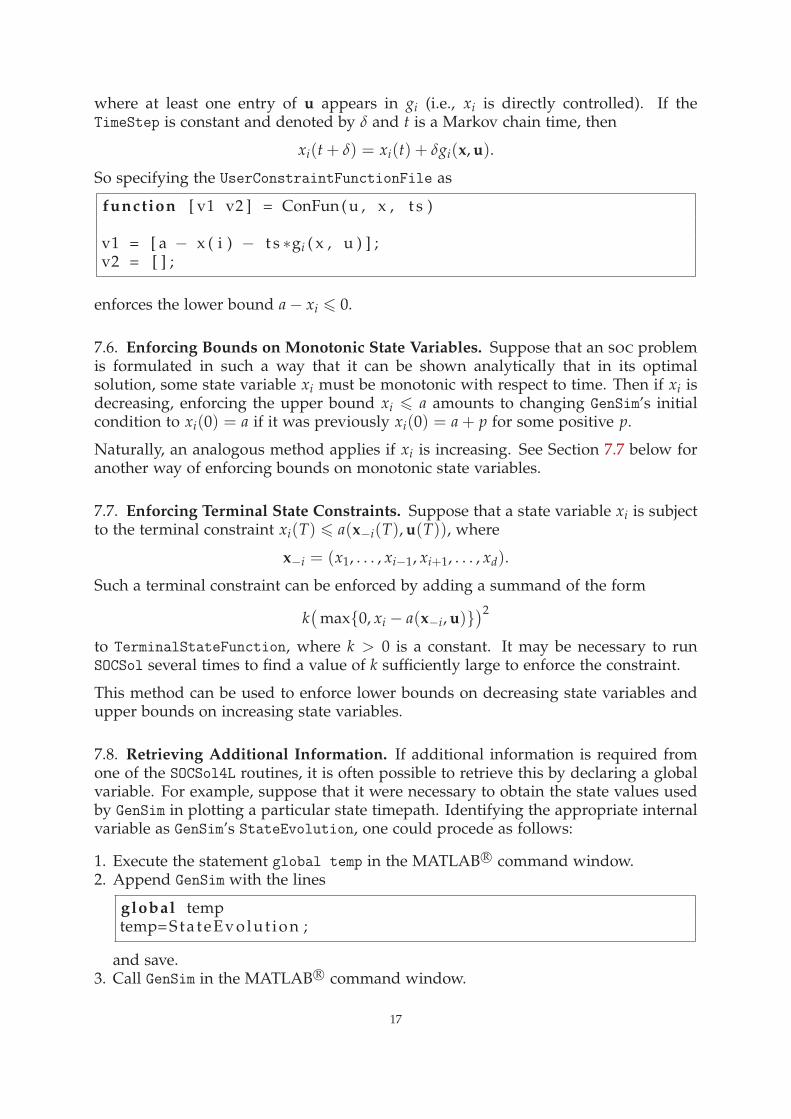
Figure 2. Control rules at time t = 0.

A.3.2. State and Control vs. Time. The files TestProblem.DPP and TestProblem.DPS areused to derive a continuous-time, continuous-state control rule. The system is thensimulated using this rule. We use the routine GenSim with the following values forthe parameters and functions described in Section 3.

ProblemFile: This is ‘TestProblem’ as before.

InitialCondition: As the simulation starts at x0 = 0.5, this is specified as 0.5.

SimulationTimeStep: For 100 equidistant time steps this is given as ones(1, 100)/100.

NumberOfSimulations, LineSpec and UserSuppliedNoise: These are not passed, asthe default values suffice.

Consequently GenSim is called as follows.

SimulatedValue = GenSim ( ‘ TestProblem ’ , 0 . 5 , ones ( 1 , 100)/100)

SimulatedValue gives the simulated value of the performance criterion. This is 0.1252(4 s.f.) with the choice of parameters given here.

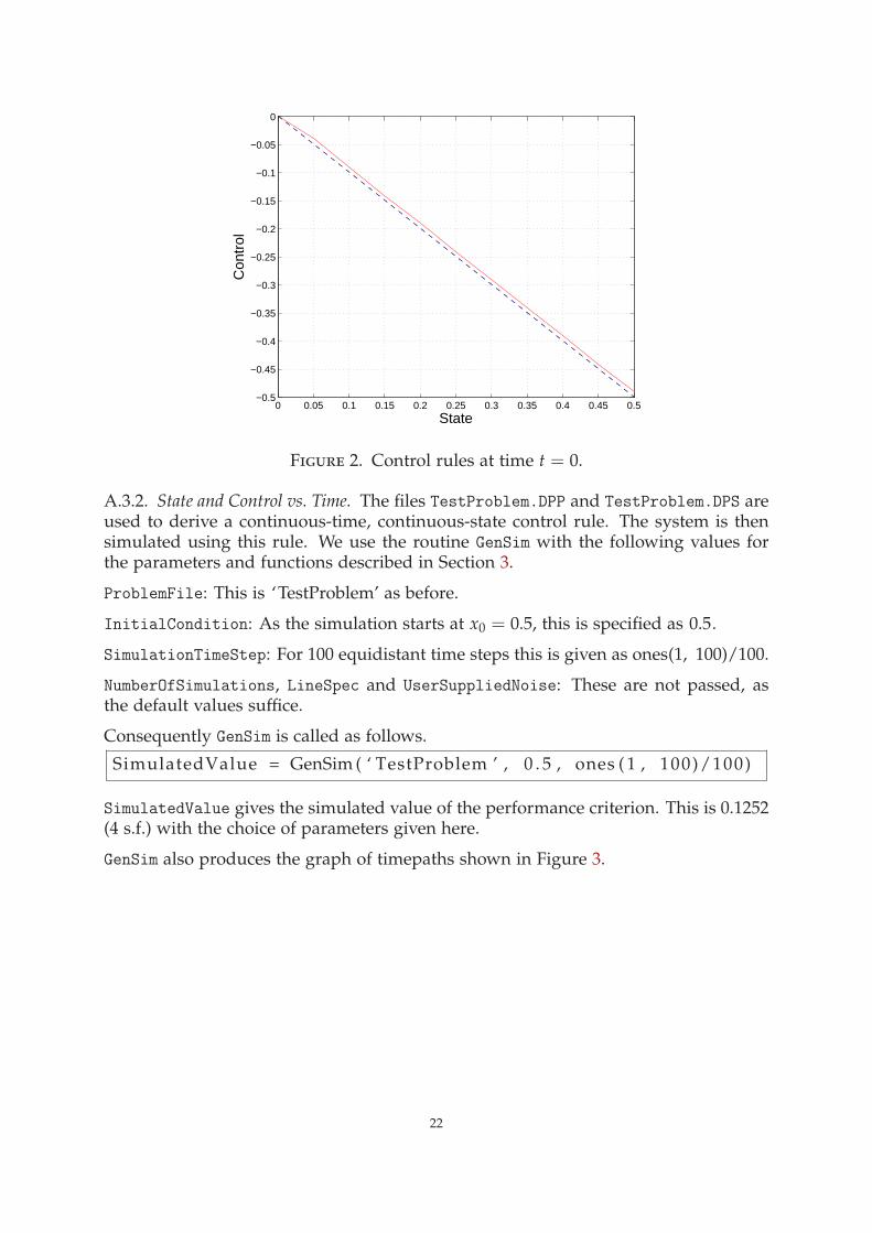
GenSim also produces the graph of timepaths shown in Figure 3.

22

0 0.1 0.2 0.3 0.4 0.5 0.6 0.7 0.8 0.9 10.1

0.2

0.3

0.4

0.5

Sta

te

0 0.1 0.2 0.3 0.4 0.5 0.6 0.7 0.8 0.9 1−0.5

−0.4

−0.3

−0.2

−0.1

Con

trol

Time

Figure 3. Optimal and approximated trajectories.

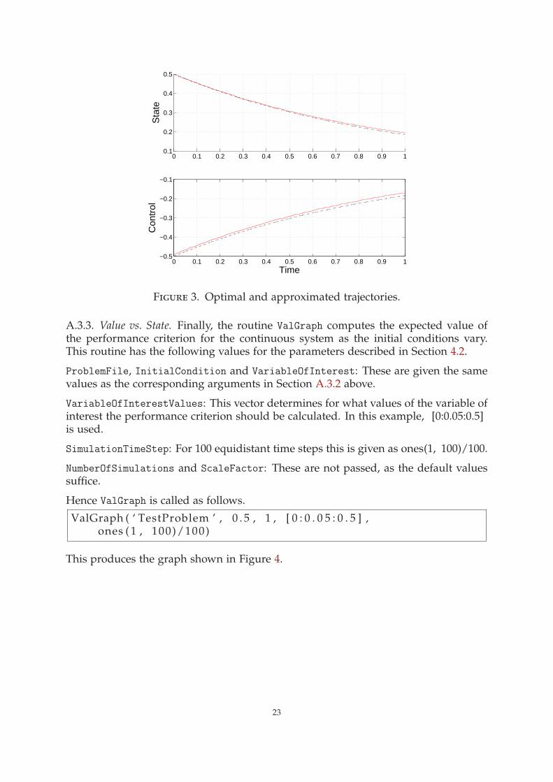
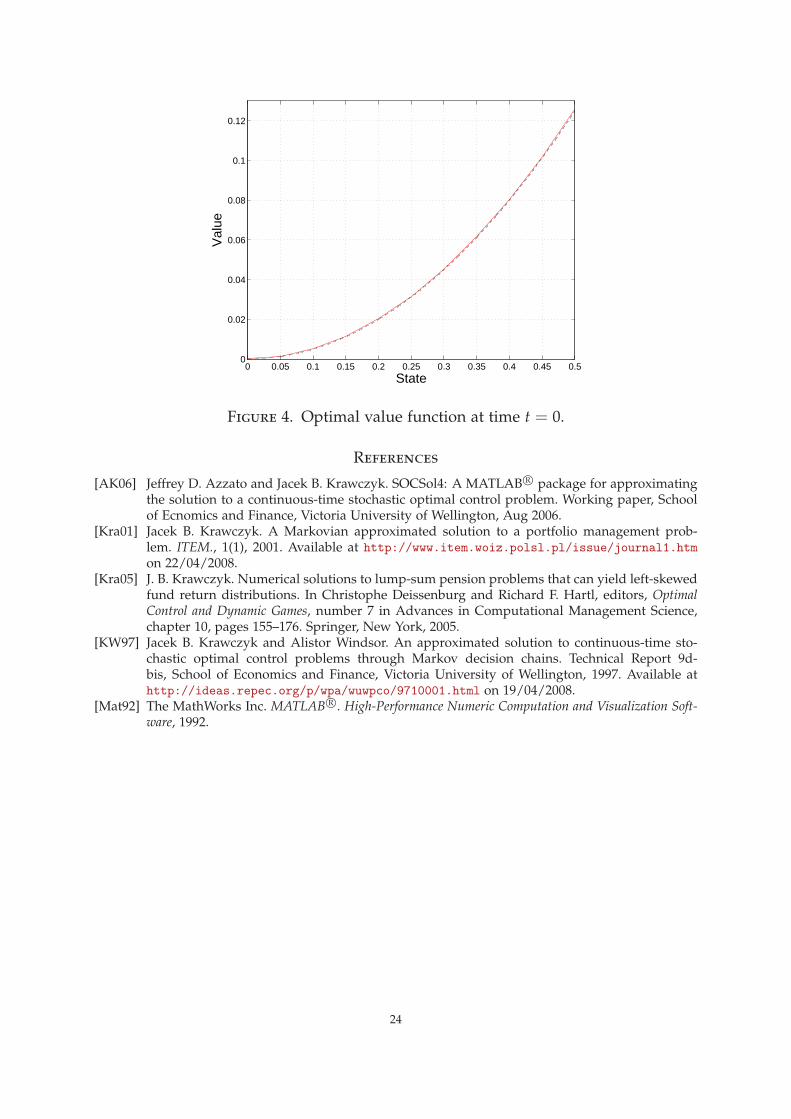
A.3.3. Value vs. State. Finally, the routine ValGraph computes the expected value ofthe performance criterion for the continuous system as the initial conditions vary.This routine has the following values for the parameters described in Section 4.2.

ProblemFile, InitialCondition and VariableOfInterest: These are given the samevalues as the corresponding arguments in Section A.3.2 above.

VariableOfInterestValues: This vector determines for what values of the variable ofinterest the performance criterion should be calculated. In this example, [0:0.05:0.5]is used.

SimulationTimeStep: For 100 equidistant time steps this is given as ones(1, 100)/100.

NumberOfSimulations and ScaleFactor: These are not passed, as the default valuessuffice.

Hence ValGraph is called as follows.

ValGraph ( ‘ TestProblem ’ , 0 . 5 , 1 , [ 0 : 0 . 0 5 : 0 . 5 ] ,ones ( 1 , 100)/100)

This produces the graph shown in Figure 4.

23

0 0.05 0.1 0.15 0.2 0.25 0.3 0.35 0.4 0.45 0.50

0.02

0.04

0.06

0.08

0.1

0.12

Val

ue

State

Figure 4. Optimal value function at time t = 0.

References

[AK06] Jeffrey D. Azzato and Jacek B. Krawczyk. SOCSol4: A MATLAB R© package for approximatingthe solution to a continuous-time stochastic optimal control problem. Working paper, Schoolof Ecnomics and Finance, Victoria University of Wellington, Aug 2006.

[Kra01] Jacek B. Krawczyk. A Markovian approximated solution to a portfolio management prob-lem. ITEM., 1(1), 2001. Available at http://www.item.woiz.polsl.pl/issue/journal1.htmon 22/04/2008.

[Kra05] J. B. Krawczyk. Numerical solutions to lump-sum pension problems that can yield left-skewedfund return distributions. In Christophe Deissenburg and Richard F. Hartl, editors, OptimalControl and Dynamic Games, number 7 in Advances in Computational Management Science,chapter 10, pages 155–176. Springer, New York, 2005.

[KW97] Jacek B. Krawczyk and Alistor Windsor. An approximated solution to continuous-time sto-chastic optimal control problems through Markov decision chains. Technical Report 9d-bis, School of Economics and Finance, Victoria University of Wellington, 1997. Available athttp://ideas.repec.org/p/wpa/wuwpco/9710001.html on 19/04/2008.

[Mat92] The MathWorks Inc. MATLAB R©. High-Performance Numeric Computation and Visualization Soft-ware, 1992.

24