University of LynchburgDigital Showcase @ University of Lynchburg

Undergraduate Theses and Capstone Projects

Spring 4-12-2019

Socioeconomic Influences of Property CrimeRates: A Study in Virginia’s CountiesMary PassleyUniversity of Lynchburg

Follow this and additional works at: https://digitalshowcase.lynchburg.edu/utcp

Part of the Other Economics Commons

This Thesis is brought to you for free and open access by Digital Showcase @ University of Lynchburg. It has been accepted for inclusion inUndergraduate Theses and Capstone Projects by an authorized administrator of Digital Showcase @ University of Lynchburg. For more information,please contact digitalshowcase@lynchburg.edu.

Recommended CitationPassley, Mary, "Socioeconomic Influences of Property Crime Rates: A Study in Virginia’s Counties" (2019). Undergraduate Theses andCapstone Projects. 129.https://digitalshowcase.lynchburg.edu/utcp/129

Socioeconomic Influences of Property Crime Rates: A Study in Virginia’s Counties

Mary Passley

Senior Research Project

Submitted for Honors in the College of Business

Department of Economics

April 12th, 2019

Dr. Gerald Prante

Dr. Michael Craig

Dr. Michael Schnur

ABSTRACT

Most research on factors and causes of crime, whether property or violent crime, focuses on individuals’ behavior or their surrounding environment. In this research, I explore the idea of socioeconomic factors correlated to property crime. I conducted a retrospective design to fully explore United States Census data and crime data gathered by the Bureau of Justice Statistics to discover statistically significant variables connected to property crime. Significant findings were shown by average people per house and retail sales per capita in all counties. Additional significant findings were percent employment change and percent with high school degree or higher in low rate counties as well as percent in labor force, percent employment change, and percent poverty in moderate rate counties. These findings may help Sheriff’s Offices allocate more research and resources to investigating why these variables affect the rate of property crime and may be able to set the rising crime rates on a decreasing trend.

I. INTRODUCTION

Economic factors are found all around society, influencing both big and small decisions. One theory, General Strain Theory, proposes the idea that socioeconomic strain pushes people to make uncharacteristically harmful choices under this strain. Economic factors such as unemployment, poverty, median gross rent, retail sales per capita, etcetera, can put pressure on people to commit crimes they would not under unstrained circumstances.

This research analyzes the pressure economic factors puts on individuals in order to determine which specific factors correlate to committing property crimes. In an effort to help law enforcement allocate time, resources, and their efforts better to combat crime, this research will determine the right economic factors to focus on to set property crimes on a decreasing trend.

In order to complete the research in a timely matter, property crimes will be represented by the number of burglaries, larceny thefts, motor vehicle thefts, and arson committed in each of Virginia’s counties. This allows the research to focus on a few, representative crimes and one state to determine the economic causes of crime which previous research has yet to do.

For a more focused approach, data will be collected for each of Virginia’s counties. More specifically, crime and demographic data from only the counties in Virginia. To keep the study concise under time constraints, crime data is coming from county Sheriff’s Offices rather than city Police Departments. Though cities may have relevant and significant findings, under a strict timeline and the vast number of cities in Virginia, it is more feasible to analyze county level data. Further research may be able to include city data as well as county data.

The decision to just research and gather data on Sheriff’s Offices was based on the idea of Sheriffs wanting to reduce crime in their counties in order to get elected. Police Chiefs are usually appointed and though they too want to reduce crime in their jurisdiction it is not as important to them as a Sheriff because they are not trying to gain votes from their community to get reelected. Therefore, in order to help the Sheriffs find ways to improve their jurisdiction and reduce crime to influence voters, this study and research will focus specifically on factors that cause crimes in counties only.

This research will be conducted in a retrospective design. Data for economic variables will be gathered from the United States Census Bureau and property crime data will be gathered from the National Incidence Based Reporting System.

II. BACKGROUND

This study is focused on property crimes such as burglary rather than violent crimes such as robbery because economic strain puts pressure on people to commit property crimes not violent crimes. All counties and Sheriffs’ Offices within Virginia self-report the data that were collected for this research study. This means, historically, that Virginia’s counties have been reporting

burglaries, larceny thefts, motor vehicle thefts, and arson the same way with the same terminology for an extended period of time. Research and studies performed on property crimes usually list various specific types of crime but this academic exploration will focus on those four crimes to represent property crime. In this study property crime(s), is the term used to address the sum of the four individual property crimes included to lessen the possible confusion between different terminology in the various studies. Each source gathered was used to support the data collected and help identify gaps that this project could correlate to the amount of property crime in each county in Virginia.

According to NIBRS (2012) the United States Census Bureau (2016) and the Bureau of Justice Statistics (2016) property crime has been rising over the last decade. To combat this issue, many research studies have been done to determine what factors are correlated to this rise in crime. One such study indicates a relationship between poverty and property crime is present, however is was unable to be determined whether property crime influenced poverty or vice versa (Lehrer 2000). Other sources pointed to socioeconomic strain as the cause of rising property crime rates (Kelly 2000). These previous studies help narrow down correlated factors of causes of property crime across the country. To combat the issue in Virginia, these studies’ findings were used to determine economic influenced factors in relation to property crime.

The data were collected from the Bureau of Justice Statistics (2016) and the United States Census Bureau (2016) so it is assumed to be reliable and valid. Krienert et. al. (2009) discussed the definition of property which was used to operationalize it for the purpose of this study. To find specific economic factors, Allison (1972) and Lauritsen et. al. (2016) were used to narrow down to the most prominent variables given the wide variety available for economic influences. Crutchfield et. al. (1997) and Gao et. al. (2017) both focus on how working and unemployment have an impact on property crime rates. Fella et. al. (2014) discussed how the education level of people in an area can have a significant impact on the amount of crime happening. Kurth (2013) discussed how socioeconomic status also influences the amount of property crime that happens in a specific area. Lehrer (2000) found evidence of poverty and crime influencing one another. Both Baron (2008) and Kelly (2000) provided previous research on how socioeconomic strain causes individuals to commit crimes to continue to provide for themselves and their families, which is the basis for Agnew’s General Strain Theory (1992). Each source gave significant information of previous findings and help further the ability of this research to fill in the gaps between them.

According to Robert Agnew’s General Strain Theory (1992), economic strains such as unemployment, poverty, and low levels of education put strain on individuals. This socioeconomic strain causes people to turn to crime to be able to provide for their families. The strain is what causes people to commit crimes they would normally not. Following Agnew’s theory, it stands to reason that counties with high percentages of poverty and unemployment, combined with low education levels should have higher crime rates because these factors contribute to economic strain (Baron 2008; Kelly 2000).

The resources, references, and studies referenced in the research will provide a foundation for finding previously linked socioeconomic factors with property crimes as well as show which factors have already been explored so this research may find new factors that are correlated to property crimes in Virginia. Finding new variables that are correlated will help police and research resources to be distributed and allotted to the factors that could help decrease the amount of crime happening in Virginia’s counties.

III. MODEL DEVELOPMENT

This study attempts to determine economic causes of property crimes in Virginia’s counties using one dependent variable made of four individual property crimes and eight independent variables.

The regression model attempts to explain high rates of property crimes in various counties of Virginia with the eight independent variables including percent of the population that possesses a high school degree or higher, median household income, percent employment change, percent poverty, percent of the population in the labor force, median gross rent, total retail sales per capita, and the number of people per household.

Increases in percent of the county population that hold a high school degree or higher should correlate to a decrease in the rate of property crimes within the county. Higher education leads to higher paying jobs, lessening economic pressure and therefore lessening the need for crimes to be committed. Higher education also predicts better rationalization of why they should not commit a crime due to the possible consequences that will affect the future. This predicts that this variable will have a negative expected sign. Running a one tailed test with a negative sign implies that the null hypothesis is β1 < 0 and the opposite being the alternative hypothesis, Ha: β1 > 0 .

Median income is predicted to have a negative sign as well because the higher the median income in a county is, the less socioeconomic strain there is on the population. This means people have a decreased desire to commit burglary to obtain needed or wanted goods. The null and alternative hypotheses for this variable is the same as for high school degree.

The coefficient of percent employment change, is predicted to be positive. A greater change in employment, assuming it is a negative change, would lead to a higher rate of unemployment and socioeconomic strain, increasing the amount of burglaries committed. The null and alternative hypotheses for a positive expected sign would be H0: β3 > 0 and Ha: β3 < 0.

As with employment change, the predicted sign of percent of poverty is positive because increased socioeconomic strains will increase the population’s desire to commit burglary to obtain more than they can afford. The null and alternative hypotheses will also be the same as employment change, H0: β4 > 0 and Ha: β4 < 0.

The next variable represents the percent of the county population that is in the labor force. It has a negative predicted sign because a higher labor force population means more people can be working to earn income which deters them from committing burglary. The null and alternate hypotheses are the same as the other negative expected signs, H0: β5 < 0 and Ha: β5 > 0.

Median rent’s coefficient is predicted to be negative based on the idea that the higher rent is in a county the higher the income, correlated with less socioeconomic strain. There is a decreased need for burglaries to be committed when people have higher incomes associated with increased median gross rent. The null hypothesis is H0: β6 < 0 and the alternate hypothesis is Ha: β6 > 0.

The predicted sign of retail sales per capita could be either negative or positive. It could be positive because higher sales provide more opportunity for people to commit burglary to obtain items they desire. On the other hand, it could be negative because higher sales per capita may indicate higher income in a particular county which provides the population with the legal opportunity to obtain wanted goods. For this study, it is assumed increased sales will increase the desire to commit burglary therefore, this study expects a positive sign. The null hypothesis for a positive sign is H0: β7 > 0 and the alternate hypothesis is Ha: β7 < 0.

The number of people per household is predicted to have a positive sign. The more people in a house, the more strain there is to provide, increasing the number of property crimes occurring. It would have the same null and alternate hypotheses as retail sales per capita.

These are the expected signs after completing research related to crimes and socioeconomic factors. However, some of the signs may not come out as predicted due to omitted or confounding variables.

IV. DESCRIPTION OF DATA

The data were collected from the United States Census Bureau on a self-reporting basis from the Sheriff’s Offices in the 86 counties in the state of Virginia. The data collected were from the 2010 Census, the reliability for this particular research design is consistent due to the previously established trustworthiness of the United States Census because the data are gathered in the same way each time, year after year. The validity for this particular research design may be credible because the source is the United States Census but the data could be collected wrong year after year, meaning it could be reliable but not valid. The United States Census Bureau is the most reliable and valid source for this data as it is gathered by the United States government. The seven independent variables come from the United State Census Bureau. The dependent variable, property crimes, comes from the Bureau of Justice Statistics and is the most reliable and valid source as it is gathered from Sheriff’s Offices in each county. Gathering the data from another source may not be reliable because the Sheriff’s Offices are the primary source for crime data in

each county and other sources would be secondary, and therefore less reliable. The data gathered for this research includes one dependent variable and eight independent variables. The dependent variable is the rate of property crimes which is calculated by dividing the sum of burglaries, larceny thefts, motor vehicle thefts, and arson in a county by the population in that county, multiplied by 1000. The eight independent variables include percent of the population that possesses a high school degree or higher, median household income, percent employment change, percent poverty, percent of the population in the labor force, median gross rent, the total retail sales per capita, and the average number of people per household. The percentages and per capita variables were already calculated by the United States Census Bureau.

V. METHODOLOGY

The proposed research design for this study is retrospective. A retrospective design allows for data to be collected by researchers in a timely manner because it has already been compiled (Salkind, 2010). Though retrospective designs look at data from the past, it is not outdated because the data being used for this study is from 2016. One advantage of this design is the data is already collected and complied so it is easily accessible and ready to use. A disadvantage of this study is factors and rates of violent crime can change every day and a retrospective design can only look at the past data.

The population for this project was the population of all the 86 counties in the Commonwealth of Virginia. There was no sample of these counties because data was available for the whole population. The setting for this research project was the Commonwealth of Virginia, which is measured as the 12th most populated state in the United States with a population of 8,411,808 as of July 1, 2016 (United States Census Bureau, 2016).

Reliability is measured by the consistency and stability of continuous measurements. “Reliability is the degree to which an assessment tool produces stable and consistent results” (Phelan & Wren 2005, p.34). The three forms of reliability are stability reliability, representative reliability, and equivalent reliability. Stability reliability basically accounts for the consistency of a source. Representative reliability relates to the sampling of data and the reliability across different subgroups. Equivalent reliability is the gathering of information in the same exact way every time; however, there are different labels for different things. For example, race came from the term ancestry. Overall, the reliability for this particular research design is consistent due to the previously established trustworthiness of the United States Census because the data are gathered in the same way each time, year after year.

Validity is a type of measurement of accuracy. “Validity refers to how well a test measures what it is purported to measure” (Phelan & Wren 2005, p.41). Face validity, content validity, and construct validity are the three forms of validity. Face validity is the reasonability of the face value of a source or data. Content validity is viewing the big picture and going in-depth with the

source to ensure the details are correct. Construct validity is testing one’s knowledge of the source and relating it to the details in the source in order to identify errors. The validity for this particular research design may be credible because the source is the United States Census but the data could be collected wrong year after year, meaning it could be reliable but not valid.

The data were analyzed through OLS, where the data were entered and formulated into frequency tables, regression models, and descriptive statistics tables. Frequency tables and descriptive statistics tables were used to convey the information held within the data while OLS and regression models were used to identify the variables that were statistically significant in this project. Statistical significance was determined by the results of the OLS regression by comparing the T-stat to the critical value as well as verifying by looking at having a p-value of less than 0.1.

VI. RESULTS

The data were run through descriptive statistics and OLS as a whole and in four separate categories. A confidence level of 90 percent was used. Table 1 details which counties are included in each category. Tables 2 through 6 detail the descriptive statistics of the counties as a whole and as individual categories. Tables 7 through 11 provide the regression output for both the counties as a whole and as separate categories.

After running the data as a whole through OLS there were two statistically significant variables found, retail sales per capita and average number of people per household. In order to find variables to be statistically significant specific to low or high rates the data were sorted into four categories based on property crime rates to determine if the counties with low, moderate, high, and very high rates had an impact.

Once OLS regressions were run within the specific data categories, two variables within one category came out to be statistically significant and three in another category. The variables that turned out to be statistically significant in low rate countries are percent of employment change and percent with a high school degree or higher. In moderate rate counties, the significant variables are percent in the labor force, percent of employment change, and percent of poverty. The significant variables are bolded and are in tables 7, 8, and 9.

There may be an issue with multicollinearity within the data. Multicollinearity can occur when two independent variables are giving very similar, overlapping data. This could be happening with the percent poverty and median income variables as both of these give information on the economic class of the individual county. However, test regressions excluding one or the other of these variables did not show substantial changes to the significant findings.

The statistically significant variables mean that there is a correlation between them and the property crime rate. These results suggest that a one point increase in the variables will lower or higher the property crime rate by their coefficient.

VII. CONCLUSION AND DISCUSSION

In conclusion, this research had some success in determining what socioeconomic factors are related to property crimes in the state of Virginia. There were a few statistically significant variables found. This research contributes an exploratory study on these significant findings. In future research the relationship between the significant variables and property crime can further be explored and researched to see if it applies to just counties in Virginia or if it would also be applicable to other states with varying rates of property crime.

With these findings, however, law enforcement can allocate resources and funding to help people that fit into a need identified by the significant variables. Sheriff’s Offices will be able to look at the correlated data to see where help can be offered. One option is to develop a program to help employment stabilization as employment change was found to have an impact on property crime rates. Another option would be to offer poverty help programs to those in moderate rate counties in an effort to reduce the amount of property crime happening there. In low rate counties, Sheriff’s Offices can work with schools to encourage students and young adults to graduate as the percent of high school graduates is correlated to the property crime rates in those counties. Raising the percent of high school graduates will help combat the rising number of property crimes.

Some recommendations for further research includes increasing the number of property crimes that represent property crimes as a whole as four crimes may have left out key findings of other significant variables. Including more independent variables may help to expand the possibility of having a statistically significant finding. If time was not an issue, including city data from Police Departments as well as Sheriff’s Offices may lead to more or different significant findings that will help determine where resources would be most effective in reducing the amount of property crimes.

TABLES

Table 1: Counties Grouped by Property Crime RatesLow(1-6)

Moderate(6.01-8)

High(8.01-11)

Very High (>11.01)

Craig Fauquier Botetourt DinwiddieMontgomery Bedford Sussex GreeneHighland Loudoun Madison LouisaCumberland Surry Dickenson AccomackBath Brunswick Bland NelsonCulpeper Essex Franklin PatrickCharles City Prince Edward Mathews LancasterNottoway Pittsylvania Wise RockbridgeRappahannock Shenandoah Augusta StaffordRichmond Alleghany Mecklenburg MiddlesexPage Northumberland Caroline King GeorgeWythe Clarke Northampton LeeLunenburg Warren Hanover BuchananRockingham Fluvanna Southampton PulaskiGiles Halifax Scott FrederickKing William Charlotte Buckingham SpotsylvaniaGreensville Powhatan Amelia New KentOrange Floyd Amherst Washington

Goochland Carroll GloucesterRussell King & Queen YorkAppomattoxSmythIsle of Wight Grayson

TazewellWestmoreland

Henry

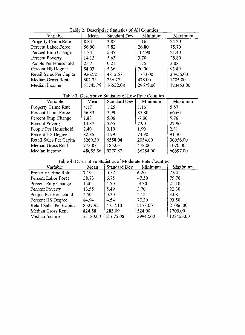
Table 2: Descriptive Statistics of All CountiesVariable Mean Standard Dev Minimum Maximum

Property Crime Rate 8.83 3.85 1.16 24.20Percent Labor Force 56.90 7.82 26.80 75.70Percent Emp Change 1.34 5.37 -17.90 21.40Percent Poverty 14.13 5.63 3.70 28.80People Per Household 2.47 0.21 1.75 3.08Percent HS Degree 84.03 5.36 70.00 93.80Retail Sales Per Capita 9262.21 4812.57 1753.00 30956.00Median Gross Rent 802.73 236.77 478.00 1705.00Median Income 51745.79 16552.08 29679.00 123453.00

Variable Mean Standard Dev Minimum MaximumProperty Crime Rate 4.17 1.25 1.16 5.57Percent Labor Force 56.33 7.99 35.80 66.60Percent Emp Change 1.83 5.06 -7.00 9.70Percent Poverty 14.87 5.65 7.90 27.90People Per Household 2.40 0.19 1.99 2.81Percent HS Degree 82.86 4.99 74.90 91.30Retail Sales Per Capita 8269.39 6558.04 2054.00 30956.00Median Gross Rent 772.83 185.03 478.00 1070.00Median Income 48055.56 9270.82 36284.00 66697.00

Table 4: Descriptive Statistics of Moderate Rate CountiesVariable Mean Standard Dev Minimum Maximum

Property Crime Rate 7.19 0.57 6.20 7.94Percent Labor Force 58.73 6.75 47.50 75.70Percent Emp Change 1.40 4.70 -4.30 21.10Percent Poverty 13.55 5.49 3.70 22.30People Per Household 2.50 0.20 2.12 3.08Percent HS Degree 84.94 4.54 77.30 93.50Retail Sales Per Capita 8527.92 4757.10 2173.00 21066.00Median Gross Rent 824.58 283.09 524.00 1705.00Median Income 55180.00 21675.08 29942.00 123453.00

Table 3: Descriptive Statistics of Low Rate Counties

Table 5: Descriptive Statistics of High Rate CountiesVariable Mean Standard Dev Minimum Maximum

Property Crime Rate 9.35 0.74 8.12 10.52Percent Labor Force 54.06 8.53 26.80 68.10Percent Emp Change 1.21 4.95 -12.90 14.00Percent Poverty 15.18 5.17 6.20 25.00People Per Household 2.44 0.20 1.75 2.79Percent HS Degree 82.71 5.63 72.30 92.60Retail Sales Per Capita 9124.27 4312.19 1753.00 18176.00Median Gross Rent 748.86 162.04 517.00 1088.00Median Income 47230.59 11375.07 33624.00 78645.00

Variable Mean Standard Dev Minimum MaximumProperty Crime Rate 13.90 2.99 11.12 24.20Percent Labor Force 58.20 7.69 40.10 68.70Percent Emp Change 1.01 6.87 -17.90 21.40Percent Poverty 13.12 6.28 5.30 28.80People Per Household 2.53 0.25 2.15 3.07Percent HS Degree 85.33 6.01 70.00 93.80Retail Sales Per Capita 11013.50 3294.84 5177.00 17187.00Median Gross Rent 857.23 278.77 507.00 1466.00Median Income 55533.86 18272.05 29679.00 97144.00

Table 7: Regression Results of All CountiesSummary Obs: 86 R2: 0.11 F: 1.24Variable β Std-Err T-Stat P-Value

Intercept -7.86 16.69 -0.47 0.64Percent Labor Force -0.16 0.11 -1.46 0.15Percent Emp Change -0.06 0.08 -0.79 0.43Percent Poverty -0.13 0.20 -0.67 0.51People Per Household 7.14 3.47 2.06 0.04Percent HS Degree 0.14 0.16 0.90 0.37Retail Sales Per Capita 0.0002 9.03E-05 1.80 0.08Median Gross Rent -2.52E-05 0.003 -0.006 0.99Median Income -6.64E-05 8.32E-05 -0.80 0.43

Table 6: Descriptive Statistics of Very High Rate Counties

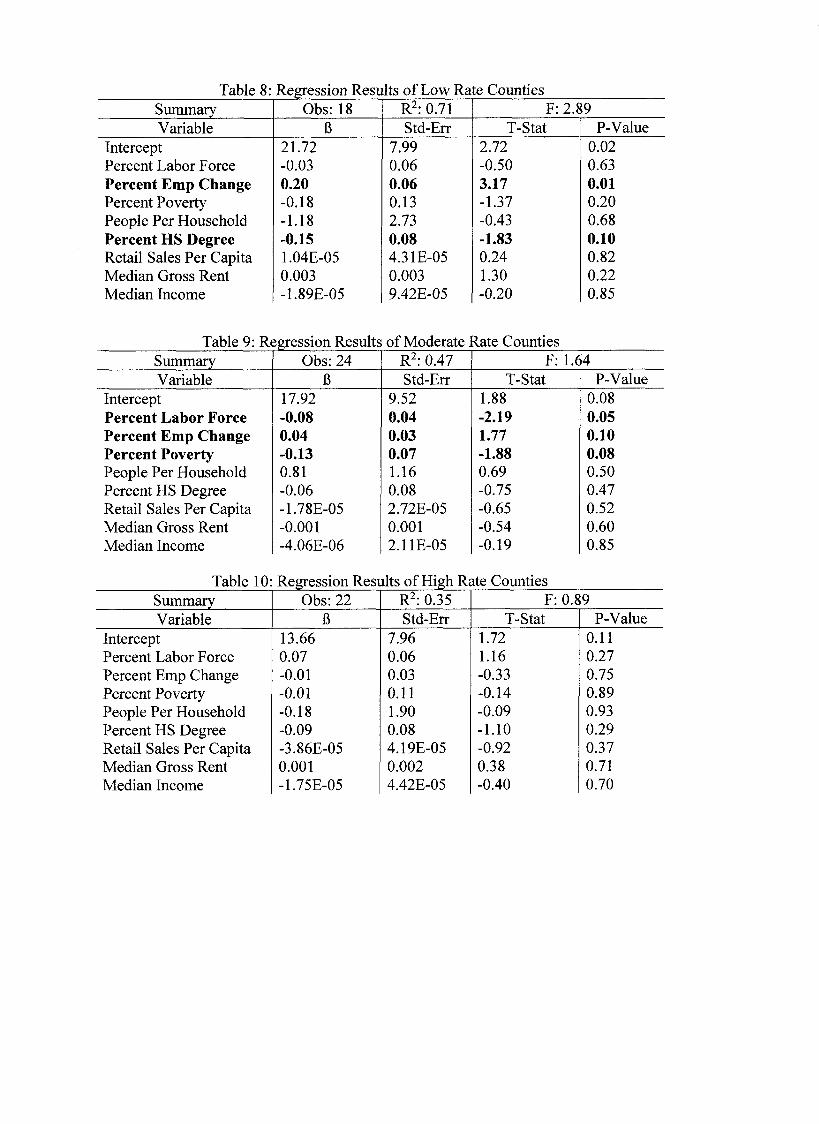
Table 8: Regression Results of Low Rate Counties

Table 9: Regression Results of Moderate Rate Counties

Table 10: Regression Results of High Rate CountiesSummaryVariable β

Obs: 22 R2: 0.35Std-Err T-Stat

F: 0.89P-Value

InterceptPercent Labor Force Percent Emp Change Percent Poverty People Per Household Percent HS Degree Retail Sales Per Capita Median Gross Rent Median Income

13.660.07-0.01-0.01-0.18-0.09-3.86E-050.001-1.75E-05

7.960.060.030.111.900.084.19E-050.0024.42E-05

1.721.16-0.33-0.14-0.09-1.10-0.920.38-0.40

0.110.270.750.890.930.290.370.710.70

InterceptPercent Labor Force Percent Emp Change Percent Poverty People Per Household Percent HS Degree Retail Sales Per Capita Median Gross Rent Median Income

21.72-0.030.20-0.18-1.18-0.151.04E-050.003-1.89E-05

7.990.060.060.132.730.084.31E-050.0039.42E-05

2.72-0.503.17-1.37-0.43-1.830.241.30

- 0.20

0.020.630.010.200.680.100.820.220.85

VariableSummary Obs: 18

βR2: 0.71Std-Err T-Stat

F: 2.89P-Value

SummaryVariable

Obs: 24β

R2: 0.47Std-Err T-Stat

F: 1.64P-Value

InterceptPercent Labor Force Percent Emp Change Percent PovertyPeople Per Household Percent HS Degree Retail Sales Per Capita Median Gross Rent Median Income

17.92-0.080.04-0.130.81-0.06-1.78E-05-0.001-4.06E-06

9.520.040.030.071.160.082.72E-050.0012.11E-05

1.88-2.191.77-1.880.69-0.75-0.65-0.54-0.19

0.080.050.100.080.500.470.520.600.85

Table 11: Regression Results of Very High Rate CountiesSummaryVariable β

Obs: 22 R2: 0.15 F: 0.28P-ValueT-StatStd-Err

InterceptPercent Labor Force Percent Emp Change Percent Poverty People Per Household Percent HS Degree Retail Sales Per Capita Median Gross Rent Median Income

-28.770.14-0.060.441.670.260.0002-0.0014.36E-06

63.220.240.170.5210.670.580.00030.010.0003

-0.460.59-0.330.860.160.450.83-0.070.01

0.660.570.750.410.880.660.420.940.99

REFERENCES

Allison, J. P. (1972). Economic factors and the rate of crime. Land Economics, 48(2), 193.

Baron, S. W. (2008). Street youth, unemployment, and crime: Is it that simple? using generalstrain theory to untangle the relationship. Canadian Journal o f Criminology & Criminal Justice, 50(4), 399-434.

Bureau of Justice Statistics. (2016). Retrieved fromhttps://www.bjs.gov/index.cfm?ty=pbdetailandiid=2218

Crutchfield, R. D., & Pitchford, S. R. (1997). Work and crime: The effects of labor stratification. Social Forces, 76(1), 93-118.

Fella, G., & Gallipoli, G. (2014). Education and crime over the life cycle. Review o f Economic Studies, 81(4), 1484-1517. doi://restud.oxfordjoumals.org/content/by/year

Gao, G., Liu, B., & Kouassi, I. (2017). The contemporaneous effect of unemployment on crime rates: The case of Indiana. Southwestern Economic Review, 44(1), 99-107. doi://swer.wtamu.edu/swervolume

Kelly, M. (2000). Inequality and crime. Review o f Economics & Statistics, 82(4), 530-539. doi:10.1162/003465300559028

Krienert, J. L., & Vandiver, D. M. (2009). Assaultive behavior in bars: A gendered comparison. Violence and Victims, 24(2), 232-47.

Kurth, W. J. (2013). Population density and rates o f at-risk behaviors o f crime and adolescent births: A quantitative correlational study (Order No. 3592909). Available from Criminal Justice Database. (1439924737).

Lauritsen, J. L., Rezey, M. L., and Heimer, K. (2016). When choice of data matters:Analyses of U.S. crime trends, 1973-2012. Journal o f Quantitative Criminology, 32(3), 335-355. doi: http://dx.doi.Org/10.1007/s 10940-015-9277-2

Lehrer, E. (2000). Crime-fighting and urban renewal. Public Interest, (141), 91.

National Incident Based Reporting System [NIBRS] (2012). Retrieved from https://ucr.fbi.gov/nibrs/2012/resources/nibrs-offense-defmitions

Phelan, C., & Wren, J. (2005). Exploring Reliability In Academic Assessment. (1), 30-47.

Salkind, N. J. (2010). Retrospective Study. Encyclopedia o f Research. (5), 34-37.

United States Census Bureau (2016). Retrieved fromhttps://www.census.gov/quickfacts/fact/table/US/PST045216