Embed Size (px)
Citation preview

Social Welfare Issues of Financial Literacy*
Professor Stephen Satchell Trinity College, University of Cambridge
Trinity Street, Cambridge CB2 1TQ, United Kingdom. Ph: +44 1223338409
Email: [email protected]
Dr Oliver Williams Scalpel Research Ltd
Abstract In the matter of financial literacy it is often supposed that more is automatically preferable to less. This paper considers to what extent this may be true generally, and specifically focuses on the case of investment forecasting skill (a significant component of an individual’s financial literacy). We show that the while improved forecasting skill can increase an individual’s own utility, the resulting increase in trading volume leads to higher asset price volatility. Under the plausible assumption that this volatility imposes disutility on non-investors, an interesting trade-off is exposed between the benefits of skill improvement which accrue to investors, and the costs suffered more broadly by society. The paper constructs a formal analytic framework in which to discuss these issues, examines under what conditions the marginal utility of skill is in fact monotonic for the individual and considers implications for policy-makers.
*The authors thank Robert Kosowski, Hamish Low and Susan Thorp for many useful comments.

Abstract
In the matter of financial literacy it is often supposed that more is automatically prefer-able to less. This paper considers to what extent this may be true generally, and specificallyfocuses on the case of investment forecasting skill (a significant component of an individ-ual’s financial literacy). We show that the while improved forecasting skill can increasean individual’s own utility, the resulting increase in trading volume leads to higher assetprice volatility. Under the plausible assumption that this volatility imposes disutility onnon-investors, an interesting trade-o! is exposed between the benefits of skill improvementwhich accrue to investors, and the costs su!ered more broadly by society. The paper con-structs a formal analytic framework in which to discuss these issues, examines under whatconditions the marginal utility of skill is in fact monotonic for the individual and considersimplications for policy-makers.
1

Social Welfare Issues of Financial Literacy
S.E. Satchell
Trinity College
University of Cambridge
O.J. Williams!
Scalpel Research Ltd
1 Introduction
“Where ignorance is bliss, ’Tis folly to be wise” Thomas Gray (1742)
“All wisdom is foolish that does not adapt itself to the common folly” Michel Eyquemde Montaigne (1533-1592)1
1.1 Financial Literacy
The topic of financial literacy has attracted a growing literature in recent years, with its relevancevery much underlined by the prominent role played by consumer finance in global credit crisesfrom 2007 onwards. The concept cuts across many diverse fields of economics, encompassingissues at the level of the individual, such as consumers’ ability to manage a household budgetor make informed decisions about credit, as well as at the aggregate level, such as the impactof financial literacy on stock-market participation (with attendant consequences for asset pricedynamics).2
A key theme of the literature is that the rapid pace of financial innovation has led to a widearray of savings, credit and investment products, provided not only by traditional institutions,but also by novel forms of intermediaries and agents (a process which has been acceleratedby technological progress, particularly the internet). Comprehending this landscape, and eval-uating competing product o!erings, has placed non-trivial demands on consumers’ analyticcapabilities, with consequently a high likelihood of sub-optimal financial decision-making. Atthe extremes, a plausible hypothesis is that the financial literati benefit from access to superiorinvestment opportunities while less well-informed members of society fall prey to predatorylending or fraudulent investment scams.
Simultaneously, financial literacy has become a prominent item on the public agenda world-wide. (Cox (2006), HM Treasury (2009) and EBF (2009) give insights into the treatment of
!The authors thank Robert Kosowski, Hamish Low and Susan Thorp for many useful comments.1quoted from ‘The Complete Essays of Montaigne’ translated by D. Frame (1957, book 3 chapter 3)2A broad overview of the field is provided by Braunstein and Welch (2002), while representative empirical
literature includes van Rooij et al (2007) who consider the relationship between financial literacy and stockmarket participation (finding that low levels of literacy are associated with low likelihoods of stock investing),Lusardi (2008) who presents evidence of financial illiteracy in the United States and Hung et al (2009) whodiscuss approaches to the definition and measurement of financial literacy itself.
2

this matter in the United States, United Kingdom and European Union respectively). Indeed,even when not stated explicitly, elements of investor education are often implicit in moves to-wards greater consumer protection in financial services, such as the Treating Customers Fairlyprinciple devised by the UK Financial Services Authority (FSA (2005)).
Whilst at first glance it might appear that more financial literacy would be unequivocallypreferable to less, it is essential to take account of how this is distributed across individuals in theeconomy. For instance it is clear that a substantial proportion of the world’s economic activityis concerned with the trading and management of financial products, and that this is executedby a highly-financially-literate technocracy. However the recent dramatic turbulence acrossfinancial markets (with severe knock-on e!ects to the real sector) vocally begs the questionof whether such a concentration of expertise is socially desirable. This discussion continuesto enjoy a particularly high profile in the popular media, e.g. Trillin (2009) (‘...having smartguys there almost caused Wall Street to collapse.’) as well as in governments across the world,exemplified by the proposal of the ‘Volcker Rule’ by Obama (2010). On a related note, withinthe academic and practitioner communities there is much debate about future performanceprospects of quantitative funds given an increasing degree of herding by investors into a relativelysmall number of correlated strategies (see Fabozzi et al (2008)).
This state of a!airs presents us with a host of intriguing theoretical problems concerningthe relationship between financial literacy, its distribution across the population and overallsocial welfare. A common thread running throughout these problems is that in each case thecentral objects of interest are the distributions of consumers’ future wealth which we can modelas depending on some vector of consumer-specific financial literacy characteristics or attributes;according to the problem at hand these might be observable quantities, e.g. age or educationallevel, or alternatively qualitative survey data (a significant body of the empirical literature dealswith such surveys, as reviewed by Hung et al (2009)). For the sake of argument we shall usethe term literacy parameter to refer to any characteristic upon which future random wealth isdependent.
In some cases these problems can be approached by applying existing well-established ana-lytic methods. For instance investigation of the impacts of sub-optimal saving and borrowingdecisions can be performed within conventional frameworks of inter-temporal consumption andportfolio choice (e.g. Campbell and Viceira (2002)). Similarly, when considering the welfaree!ects su!ered by consumers who do not make full use of certain financial products (either bychoice or due to lack of information), we can find a starting point in the literature which dealswith the e!ects of portfolio constraints, e.g. Vila and Zariphopoulou (1997) consider the impactof borrowing constraints while He and Pearson (1991) address short-selling constraints.
However many important problems remain which are somewhat specific to this domain. Tothat end, in this paper we present general results concerning the relationship between financialliteracy and individuals’ expected utility as well as complementary results at the aggregatesocial level. Furthermore, as a topical example, we focus attention on one particular attributeof literacy which is investment forecasting skill.
There are many aspects of forecasting skill embedded in the concept of financial literacy. Aswe have already declared, financial literacy problems are often characterised by a random distri-
3

bution of future wealth and forecasting skill concerns how well an individual can anticipate theserandom future outcomes. In its broadest sense the notion is very flexible, for instance a family’sdecision over whether to rent or buy a house will (to some extent) depend on their expectationof future house price inflation, while their choice of a fixed or variable rate mortgage dependson expectations of the path of future interest rates. Similarly, decisions about investment inhuman capital (e.g. higher education) depend on expectations of future earnings, which in turnrelate - to some degree - to broader macroeconomic factors. The apposite issue here is that thevast majority of individuals are engaged in a forecasting process at some point in their lifetimesand that their e!ectiveness in this process is influenced by their level of financial literacy.
Notwithstanding the variety of themes which come under the forecasting umbrella, we de-vote our attentions here to the example of forecasting future asset prices from an investmentperspective, since this is one of the most prominent and explicit forecasting processes in whichan individual might participate. Nevertheless, a substantial proportion of households in ad-vanced economies typically ‘outsource’ this forecasting problem to professional fund managers.Within that industry active, rather than passive, management of assets is often equated withforecasting skill and presumably active managers are highly financially literate. Their skill at-tracts fees and underpins a large part of the financial industry however their claims to be able topredict financial outcomes are controversial and their activities are from time to time deemed tobe prime examples of the negative e!ects of ‘too much’ financial literacy in the ‘wrong hands’.This raises the specific questions of what level of forecasting skill is desirable and how shouldthis be distributed in the population. These issues are clearly of both academic and politicalinterest and in this paper we set out a framework in which to address them.
1.2 Investment Forecasting Skill
Discussion of asset price predictability has raged in the economics and finance literature forcenturies. Contributions range from the technical analysis methods devised in 18th centuryJapan3 to the e"cient market hypotheses debates throughout the 20th century (e.g. Bachelier(1900), Fama (1965), Samuelson (1965), Malkiel (1973)) and more recent work on behaviouralfinance (Kahneman and Tversky (1979), Simon (1987), Shleifer (1999)). Regardless of whereone stands on this topic it is evident that investors’ appetite for actively managed funds hascontinued unabated and their trading activities constitute a vast proportion of everyday financialmarket turnover.
Against this background an orthodoxy has developed in certain political-economic quartersas regards the preferred structure of financial markets. For instance arguments are frequentlyadvanced in favour of wider household ownership of equities (often connected with privatizationschemes, e.g Perotti (1995)), greater control by individuals of their pension portfolios (Em-merson and Wakefield (2003)) and investment by the general public in hedge funds (e.g. FSA(2005)). In many jurisdictions this has led to the implementation of specific policy measureswith profound consequences for the asset management industry as well as the welfare of indi-viduals themselves. From the point of view of financial economics, a major substantive impactof these measures is to alter the distribution and levels of forecasting skill among investors. As
3the so-called Sakata Rules reputedly devised by rice trader Munehisa Homma
4
the dramatis personae of markets change, so too does the character of their price dynamics.From a theoretical perspective, an extensive body of literature demonstrates how active trad-
ing can lead to increased volatility; this trading may itself be the result of superior infomation(Grossman and Stiglitz (1980)), opportunistic ‘noisy’ behaviour (Campbell and Kyle (1988),De Long et al (1990)) or fundamental analysis (Graham and Dodd (1934)), but all of thesechannels involve some component of skilled forecasting.4 However when investors are relativelyunskilled they may have no conscious forecast whatsoever or, if they do, update it erroneouslyand infrequently. Under relatively undemanding assumptions about rationality on the part ofinvestors, low skill translates into negligible trading and, in turn, less volatile markets. Withthis in mind, the supposition that such policies are a ‘good thing’ sits uneasily with the intuitionthat they may bring increased volatility in their wake.
In the sections which follow we specifically set out to address two broad groups of policyquestions which we categorise as follows:
Type I questions concern the level of skill in the market: What is the optimal level of skillwhich an investor should attempt to attain? Is more skill always preferable to less skill? Is itsocially desirable to increase the level of all investors’ skill in general? These are relevant todiscussion of financial literacy and investor education.
Type II questions relate instead to the distribution of skill: Is it in the interests of unskilledinvestors to delegate portfolio decisions to professional managers with superior skill? Is therea socially-optimal allocation of capital across di!erentially-skilled investor types? These arerelevant to financial product innovation (e.g. introduction of 130/30 funds) and broadeningretail access to more sophisticated products such as hedge funds.
The importance of Type II questions is sharpened by the observation that many famousfinancial catastrophes (e.g. Barings, Long Term Capital Management and Mado!) have in-volved one group of investors accepting uncritically a real (or imaginary) complex, mathematicalderivatives strategy purveyed by another group, supposed to have superior skill.5
Our results are illuminating: we find that increasing the skill level of one group of investorscan indeed increase their own utility but the induced incremental volatility can simultaneouslyreduce the utility of others with a net impact on social welfare which is negative. We also findthat even if competing groups of independent investors increase their level of skill in tandem itis perfectly plausible for overall welfare to decline; once again the culprit is increased volatility.
Existing theory provides us with helpful foundations from which to select appropriate literacyparameters ! to represent skill. While it is common practice to measure managers’ ex postperformance with metrics such as Sharpe ratios and Information Ratios these do not di!erentiatebetween returns achieved due to luck or forecasting skill. Fortunately, however, a range ofalternatives is available which measure managers’ forecasting ability directly; as well as beingrevealing statistics as regards skill we find that these parameters also have valuable economiccontent and indeed define skill as a quasi-commodity over which preferences can be establishedmuch like conventional goods.
4Value investors used to claim that their skills involved no notion of forecasting outside pure arbitrage, butthe notion of value involves some projection of future earnings in most cases.
5See Fay(1997), Lowenstein (2001) and Markopolos (2010) for explanatory accounts of Barings, LTCM andMado! respectively.
5

Our approach is to first construct a general equilibrium model of agents with heterogeneousskill levels and solve for equilibrium prices and portfolios conditional on agents’ respectiveproprietary forecasts. We then examine the resulting distributions of equilibrium price, wealthand utility over repeated forecasting instances. This gives us an ex ante picture of the relativemerits of di!erent market structures (in terms of agents’ skill levels).
Existing literature treats the topic of performance measurement extensively; for instanceBain (1996) reviews methods from a practitioner viewpoint, Aragon and Ferson (2006) reviewtheory and recent empirical evidence and Knight and Satchell (2002) covers a range of theo-retical and practical themes. A separate branch of literature considers the appropriateness ofperformance measures and their relationship to the investor’s optimal portfolio constructionproblem (e.g. Leland (1999)). Notwithstanding these contributions we believe that this paperis among the first to address the topic of skill from a marginal utility or welfare perspective.
Much of the literature on dynamic models with heterogeneous investors deals with the casewhere agents are all price-takers. Examples include Detemple and Murthy (1994) and Zapatero(1998). These models feature exogenous primitives such as stochastic production processes andderive equilibrium interest rates which typically have a weighted average form dependent oninvestors’ asymmetric beliefs and evolution of wealth. However the e!ect of interaction on riskyasset prices is limited or nonexistent. For example, agents decide what quantity of capital tocommit to alternative available investments based on an imperfect returns forecast however theactual return does not respond to the quantity demanded, rather the demand e!ect shows upin the equilibrium rate of return of the risk-free asset which soaks up residual wealth.
For our purposes it is essential to capture the notion of competition between agents forreturns. Introducing non-price-taking behaviour into conventional continuous-time dynamicmodels is a complex undertaking in its own right, and Basak (1997) remains one of the fewtreatments of this problem. In view of the rich heterogeneity which is central to our analysis wefocus here on static models which nevertheless expose our key results. Heterogeneity in staticmodels has remained relatively unexplored for some time; Lintner (1969) covered much of therelevant ground in a non-price-taking model. We find that introducing forecasting skill into thiscontext brings useful new insight and we look forward to extending this to a dynamic settingin future work.
The organisation of the paper is as follows: in section 2 we introduce our central financialliteracy propositions cast in a general risk-sharing framework, in section 3 we present a modelof two discrete wealth states in which financial literacy is characterised using hit-rate as aforecasting skill measurement and in section 4 we apply the model to the policy questionsoutlined above. Section 5 concludes, considering the relevance of our findings for empirical workand areas for further study. Proofs and detailed derivations are relegated to the Appendix.
6

2 Financial Literacy: Individual Utility and Social Welfare
2.1 Individual Expected Utility
Suppose we have K agents: each has a private signal S(i) which is jointly distributed (accordingto their subjective belief) with the actual state of the world which we denote by z. This jointdensity is denoted q(S, z) where S is the vector of all agents’ signals. For the sake of clarity ofnotation we have that all securities are in zero net supply and all cashflows are settled in thesame period, i.e. the payo!s of securities occur at the same point in time as their settlement.Finally, each agent’s joint distribution q depends on a literacy parameter !(i) and we denote by! (no superscript) the vector of all agents’ skill parameters together.
The agents trade with each other and construct optimal portfolios of wealth in all stateswhich we represent by the function w(i)(S, z; !). We make no assumptions on the form which w(i)
might take. We do not explicitly solve here the optimization problem to determine w(i)(S, z)(which is well-established elsewhere in the literature, dating back as far as Wilson (1968)),however in order to understand what follows it is essential to note that w represents the state-dependent wealth of the agent in equilibrium. Also, due to the single period nature of our model,w(i) is the agent’s final wealth net of the initial cost of securities and this will clearly dependon the entire vector of literacy parameters in the market (!) since these influence the individualdemands of other agents.
We begin by considering the perspective of an individual agent. For clarity in the algebrawhich follows we tend to suppress the (i) superscripts.
Proposition 2.1. Marginal expected utility of the general literacy parameter !i is given by:
E [uw(w(S, z; !))w!(S, z; !)] + COV!u(w(S, z; !)), q!(S,z;!)
q(S,z;!)
"(1)
Proof. See Appendix.
Clearly a su"cient condition for positive marginal expected utility of literacy will be havingboth terms positive and we consider these individually below.
The first term in (1) is the marginal expected utility of a literacy improvement while keepingthe subjective density unchanged, i.e. we focus only on the influence which the literacy param-eter has on position size (and hence future state-dependent wealth). For instance: a literacyimprovement might take the form of an increase in forecasting skill which reduces the disper-sion of an agent’s future state distribution; ceteris paribus, depending on the precise form of theagent’s utility function, that increase in precision may lead to the agent altering his portfolio,increasing positions in states believed to be more likely (and reducing positions in less likelystates). However whether or not this also leads to an increase in the agent’s expected wealthdepends on the demand function(s) of other agent(s) and the resulting equilibrium price. Theoverall e!ect of this entire interaction is concentrated in this term which we call the sizing term.
In Figure 1 we provide a simple example. Here we have two agents A and B and a singlerisky asset. Each agent has a CARA utility function with equal risk aversion (") and theyeach believe that the future asset price is normal although they di!er as regards its mean and
7

Figure 1: A simple example of interacting asset demands between two agents with heterogeneousforecasts of the future price; A0A"
0 and A1A"1 are demand schedules for agent A at two di!erent
skill levels and BB" is the supply schedule for agent B (obtained by reflecting agent B’s demandschedule in the price-axis). Equilibrium prices are pi and the mean forecasts of the agents aremA and mB. At both equilibria agent A is a seller of assets while agent B is a buyer (representedgraphically as a supplier of a negative quantity).
variance. It is straightforward to show that their resulting demand for the risky asset is linearand given by Qi = mi#p
"#2i
where mi and #2i denote type-specific forecasts of mean and variance
(with i either A or B) and p is the equilibrium price.6 In the figure the individual agents’ assetdemands are represented by the lines AA" and BB". Evidently a skill-increasing improvementin literacy (reflected in a decrease in #2
i ) causes a flattening in these lines although they willalways intersect the price axis (where Q = 0) at the respective mean forecast level mi.
Hence we see that improving type A’s literacy (flattening the line from A0A"0 to A1A"
1)increases the quantity of securities sold by agent A in equilibrium. However note that agentA’s expected wealth depends not only on this quantity but also on the equilibrium price. Thisexpected net wealth (before and after the flattening) is illustrated on the graph by the appro-priate shaded box (bordered vertically by the lines Q = Qi and the p-axis, and horizontallyby the lines p = mA and p = pi). Clearly increasing the equilibrium traded quantity Qi (inabsolute terms) does not necessarily increase expected wealth as this will depend on the preciseshape of the other agent’s demand schedule (e.g. BB"). This is why the sign of the sizing termis of particular interest.
The second term in (1) is the covariance between utility of state-dependent wealth andthe ratio q!(S,z;!)
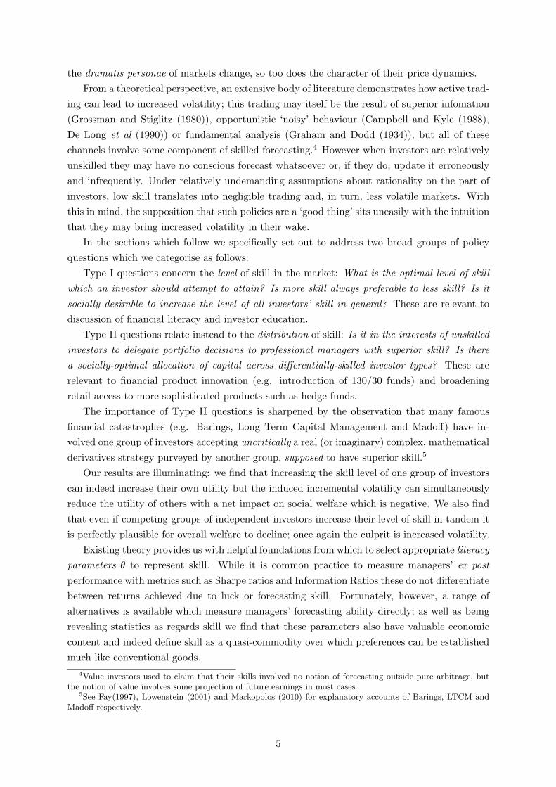
q(S,z;!) (this ratio could approximately be thought of as the proportionate ‘distortion’applied to the joint density function q at point (S,z) when the literacy parameter is increased byone unit). For instance, suppose we consider the conditional q(z|S) to be a standard univariatenormal and treat the literacy parameter as a skill-induced precision adjustment to the (unity)
6A detailed derivation is provided by Williams (2009).
8
Figure 2: A simple example of a density ‘distortion’ function based on a standard normal where! = 4 plotted over the domain (!0.4,+0.4)
variance, i.e. variance is defined as#
1!
$2, then we have:
q(z; !) = !$2$
exp!! !2z2
2
"
q!(z; !) = q(z;!)! ! 2!z2q(z;!)
2q!(z;!)q(z;!) = 1
! ! !z2
which we illustrate in Figure 2 for the case ! = 4. Positive values of the ratio occur wherethe density is ‘pulled upwards’ by the improvement in literacy (indicating relatively more likelystates) and negative values where the density is ‘pushed downwards’ (indicating the opposite).We are interested in the value of the covariance between this function and the agent’s statedependent utility. Ideally, given an improvement in literacy d! and knowing their private signalS, the agent would adjust their portfolio in perfect sympathy with the ‘distortion’ function(e.g. overweighting positions where ‘distortion’ is positive and underweighting where negative),leading to a positive covariance. This term therefore represents how closely state-dependentutility is ‘tuned’ to the ‘improved’ subjective density belief which the agent obtains. We callthis therefore the tuning term.
We next present an example of a special case which helps to provide some intuition.
Corollary 2.2. Suppose that the agent’s wealth is unconditionally normally-distributed, thenthe condition for positive marginal expected utility of the general literacy parameter !i is:
COV!w, q!
q
"+ E [w!]
COV [w, w!]> RA
where RA is Rubinstein’s (1973) coe"cient of global risk-aversion.
Proof. See Appendix.
Various remarks follow from this corollary:(a) As regards E [w!]: positivity of this term by itself is neither necessary nor su"cient for
(2.2) to hold. This is the very essence of our proposition: an increase in literacy which increases
9
future wealth on average is not guaranteed to deliver net positive marginal utility once otherdistributional characteristics are taken into account.
(b) The ‘tuning’ e!ect represented by COV!w, q!
q
"can take any sign depending on the
precise relationship between the nature of the investor’s literacy parameter (as it influences thesubjective distribution q) and the flexibility which is available to construct the state-dependentportfolio w. For instance (returning to the example where ! represents forecasting skill) ifthe agent is in the unfortunate position of skillfully forecasting parts of the distribution whichcannot be traded using available securities (e.g. extreme events in the tails of the distribution)then this term could be negligible. In the opposite case of a complete market with no portfolioconstraints we would expect this term to be positive.
2.2 Social Welfare
We now turn our attention to the overall profile of financial literacy in the market and itsrelationship to an equally-weighted social welfare function. We begin by assuming a numberof heterogeneous investor types, each with potentially di!erent initial wealth levels (denotedw0) and utility functions. We define a cross-sectional distribution of agent types according toheadcount, which we denote by f , and for each agent type we denote the j’th moment of theiruncertain wealth gains by M (j)(!). Note that these moments are a function of the entire profileof literacy in the market represented by the vector of all agents’ literacy parameters !. For eachtype we also assume the existence of all derivatives of their utility function, where we denotethe j’th derivative by u(j).
Hence, from a cross-sectional point of view, we can think of both u(j)(w0) and M (j)(!) asrandom variables with values which depend on the type of a randomly-selected agent, distributedaccording to f .
Proposition 2.3. For an economy with an equally-weighted Social Welfare Function we definethe Social Benefit of Trading (SBT ) as the incremental social welfare achieved in equilibriumas a result of securities trading among agents with a profile of literacy !. This is given by thefollowing expression:
SBT (!) =%%
j=1
Ef
&u(j)(w0)
j!M (j)(!)
'
where Ef indicates expectation taken with respect to the cross-sectional distribution of agenttypes (f) and u(j) and M (j) are cross-sectional random variables as described above.
Proof. See Appendix.
Corollary 2.4. For an economy composed of multiple types of investor where future wealth isnormally-distributed we have
SBT (!) = COVf
(u"(w0), µw(!)
)+
12
Ef
!u""(w0)M (2)(!)
"
where µw(!) " M (1)(!) and M (2)(!) respectively denote the type-specific mean and second mo-ment of wealth gains, both of which are cross-sectional random variables distributed according to
10

f . COVf and Ef denote covariance and expected value calculated across types in the populationwith respect to this f distribution.
Proof. This follows from Proposition 2.3 by noting that Ef [µw(!)] = 0 due to market clearing7
and hence Ef [u"(w0)µw(!)] = COVf [u"(w0), µw(!)].
This corollary shows us that for risk averse agents (u""(w0) < 0) a necessary conditionfor positive SBT is that initial wealth covaries negatively with expected wealth gains acrossinvestor types. In other words we require that wealth enhancements due to literacy will accrueon average to the poorer members of society. Taking the particular example of investing skill:although we lack empirical evidence on this point we suspect that this covariance is more likelyto be positive in reality, i.e. it is the wealthier investors in society who have the means toeither improve their own skill or to delegate management of their funds to others with superiorskill. Were our suspicion to be true, it would turn the sign of the first term negative in (2) andthereby militate against any social benefit of skill.
The corollary also gives us conditions under which changes in the profile of financial literacywill be socially beneficial. For instance if society has a choice between two alternative profiles!1 or !2, both of which result in an equal cross-sectional second moment of wealth, then !1 willbe preferred if
COVf
(u"(w0), µw(!1)
)> COVf
(u"(w0), µw(!2)
)(2)
Corollary 2.5. For an economy composed of multiple types of investor with identical utilityfunctions u where future wealth is normally-distributed and initial wealth is equal across all thetypes we have
SBT (!) =12
Ef
!u""(w0)M (2)(!)
"(3)
Proof. This follows immediately from Corollary 2.4 above where the first term becomes zerowhen u"(w0) is equal across all types.
For risk averse investors the sign of SBT in (3) will be unambiguously negative since M (2) >
0. However in a no-trade equilibrium we have zero mean and variance of wealth gains sincefuture wealth equals initial wealth. The immediate consequence of this is that society wouldprefer an equilibrium with absolutely no trading (M (2) = 0) to any equilibrium with trading(M (2) > 0). Returning to our example where ! represents forecasting skill: if we assume that allunskilled investors have identical di!use beliefs about future prices (resulting in zero trading)then this would be equivalent to a preference for no skill over any skill.
In summarising the results above it is clear that general arguments will be hard to find,therefore we consider further particular special cases in the section which follows. These willdemonstrate the applicability of our propositions. Prior to that exposition however we brieflydiscuss parametric measurements of forecasting skill from a more practical viewpoint.
7Securities are in zero net supply hence aggregate demand equals aggregate supply ex ante and once uncertaintyis resolved the value of aggregate profit will equal the absolute value of aggregate loss. Informally-speaking,trading is a ‘zero sum game’ in this model.
11

2.3 Forecasting Skill Metrics in Practice
Before we proceed to model forecasting skill as a particular attribute of financial literacy, itis instructive to briefly review candidates for the parameter which we have thus far labeledas !.8 The fundamental requirement is that ! should be some measurement of dependence orassociation between actual future states of the world and a forecast which is made at the timewhen asset demands are determined. We outline two possibilities below.
2.3.1 Hit-Rate
Perhaps the simplest measure of association in this context is the hit-rate which we can defineinformally as the proportion of forecasts which are directionally correct. Here we ignore magni-tudes of return entirely and focus simply on the signs of the forecasts and actual outcomes. Ina basic incarnation we might consider a model of two discrete states which we represent by theoutcomes 0 and 1 respectively and denote by the random variable Q. We also restrict forecaststo be correspondingly either 0 or 1 and denote these by the random variable S. For the sake ofparsimony we assume that the hit-rate is not conditional on the direction of the forecast (i.e. 0forecasts are equally-likely to be correct as 1 forecasts) and therefore we define the hit-rate as:
P[Q = 1|S = 1] = P [Q = 0|S = 0] = h
2.3.2 Information Coe!cient
Grinold and Kahn (1999) define the Information Coe"cient (IC) as the correlation betweenan investor’s forecast of a future asset return (in terms of a standardised score) and the actualreturn where return is defined as
rt+1 "Pt+1
Pt! 1
Formally, if we were to represent the forecast as a standardised normal random variable, S #N(0, 1), unconditional expected future return as µ, and assume joint-normality between forecastand actual return rt+1, then the conditional forecast return would be:
E[rt+1 | S] = µ + IC#S
where IC is the investor’s Information Coe"cient and # is the unconditional standard deviationof the return. Similarly we obtain the investor’s conditional forecast variance:
V ar[rt+1 | S] = #2(1! IC2)
The Information Coe"cient features extensively in the portfolio management literature. Byway of examples: Coggin and Hunter (1983) discuss empirical IC measurement issues, Dimsonand Marsh (1984) refer to the concept in their empirical study of analysts’ forecasting ability,Khan et al (1996) apply IC in global asset allocation, Khan (1998) discusses its applicability
8A detailed discussion of skill measurement is beyond the scope of this paper. More complete treatments ofthis topic are provided by Aragon and Ferson (2006), Granger and Machina (2006) and Williams (2009) amongothers.
12

in bond investing, Lee (2000) uses it as a key parameter in a range of analytics pertaining totactical asset allocation, Herold (2003) discusses its relevance in qualitative forecasting, Satchelland Williams (2007) consider the question of optimal forecasting horizon and Fishwick (2007)analyses the case of multiple models.
For purposes of reconciliation we provide the proposition below as a rule-of-thumb to aid incomparison of hit-rates and Information Coe"cients.
Proposition 2.6. For the case of forecasting a future state which takes only one of the twodiscrete values 0 or 1: if forecasts are also restricted to the discrete values 0 and 1 wherethe probability of a forecast of 1 is denoted by g, then the relationship between hit-rate h andInformation Coe"cient (IC) is given by:
IC =h! g
1! g
For example when g = 12 then IC = 2h! 1.
Proof. See Appendix.
In the analysis which follows we have chosen to focus on the use of hit-rate as a skill mea-surement within the context of a two-state model. Equivalent analysis for the case of theInformation Coe"cient (with a continuum of states) is more involved but raises several furthersubtle insights. We consider the IC case in a separate paper9 where, despite the incrementalcomplexity, we find several results which are qualitatively similar to those which follow in thispaper.
3 A Model with Two Discrete States
3.1 The Model and Equilibrium Solution
Suppose we have K agents, divided into two types (A and B), two states of the world and asingle risky asset which pays o! one unit in state 1 and zero units in state 0. We denote theactual probability of state 1 by g and the proportion of agents who are type A by $ (with0 < $ < 1). Each agent receives a type-dependent private signal SA or SB and has a hit-ratehA or hB which represents the probability of their signal being correct. Therefore for each agentwe need to solve the expected utility maximisation problem to obtain the quantity of risky assetwhich they buy given their signal. We denote this quantity x0 (when S = 0) or x1 (when S = 1).We assume the agents have exponential utility functions with di!ering risk aversions "A and"B and to ease the algebra we make the additional assumption that each agent can borrow andlend unlimited amounts at a risk-free rate of zero.10
9Satchell and Williams (2010)10While clearly unrealistic this allows us to highlight key details in the model which concern forecast formula-
tion, price determination and utility realisation. Including more complex heterogeneity in wealth and preferencesis straightforward and does not significantly alter the basic results we present here.
13

Furthermore all settlement and payo!s take place in the same time period so the assets havethe character of futures-type contracts. We denote equilibrium price by p and hence agents’expected utilities (conditional on their signal) are given by:
E [U |S = 0] = ! 1"
(1! h) exp [!"x0(1! p)]! 1"
h exp ["x0p]
E [U |S = 1] = ! 1"
h exp [!"x1(1! p)]! 1"
(1! h) exp ["x1p]
Optimal position amounts x are easily found by di!erentiation:
dU0
dx0= (1! p)(1! h) exp [!"x0(1! p)]! ph exp ["x0p] = 0
xS=0 =1"
log*
1HP
+
dU1
dx1= (1! p)h exp [!"x1(1! p)]! p(1! h) exp ["x1p] = 0
xS=1 =1"
log*H
P
+
where for convenience we refer to the probabilities in terms of odds:
H =h
1! h
P =p
1! p
and for notational clarity these quantities will often feature in our expressions instead of theunderlying probabilities. If the signal S = 1, for instance, then the odds ratio H
P can beinterpreted as indicating the agent’s level of optimism or pessimism relative to the market.
The equilibrium price p is now found by imposing market clearing. As an example weconsider below the case where SA = 0 and SB = 1:
$
"Alog
*1
HAP
++
1! $
"Blog
*HB
P
+= 0
*1
HAP
+ "#A
=*
P
HB
+ 1""#B
P =(HB
)1""#B
"#A
+1""#B
*1
HA
+"
#A"
#A+1""
#B
P =(HB
)1#f*
1HA
+f
where superscripts and subscripts index H and " according to agent type and we use f to denotethe risk-tolerance weighted proportion of type A’s in the market. We note also that 0 < f < 1and that when "A = "B (i.e. we have common constant risk aversion between the two agenttypes) then f and $ are equal. Given our assumption of constant absolute risk aversion it isclear that an increase in risk-aversion of type i is equivalent to a reduction in the proportion oftype i agents in the market. Therefore much of the following analysis proceeds in terms of the
14

f parameter without discussion of any di!erential risk aversion between agents.11
In all we have four cases to consider depending on values of SA and SB and the correspondingsolutions appear in Table 1 where in the interests of tidy notation we define M = (HA)f (HB)1#f
and Q = (HA)f (HB)f#1.
Table 1: Equilibrium in two-agent two-state model, conditional on each agent having formedtheir forecasts but before state of the world is revealed
SA, SB P p0, 0 1
M1
1+M0, 1 1
Q1
1+Q
1, 0 Q 11+ 1
Q
1, 1 M 11+ 1
M
3.2 Equilibrium Price and Wealth Dynamics
Although our model is inherently static it can be thought of as a transmission mechanismwhere agents’ signals (either 0 or 1) are converted into equilibrium price. In this sense it isapparent that equilibrium price dynamics are driven by the changing nature of agents’ beliefsover time. Given knowledge of the agents’ skill levels (as embodied in h) along with furtherdetails of the probability distribution of forecasts and outcomes we can gain insight into plausiblecharacteristics which the unconditional price distribution may have over time. (Here we interprettime to mean a series of repeated forecasting instances.12)
In order to fully specify the joint distribution of (SA, SB, z) it remains for us to specify themarginal univariate probabilities of SA and SB and also the nature of dependency between them.We consider simple extreme examples below but note that more complexity could potentiallybe incorporated here, for instance via copula-type representations (e.g. Tajar et al (2001)).
It is essential to note that the dependence structure assumed between the agents’ signalsplaces strict constraints on values which hA and hB can take, e.g. it is nonsense for both hA
and hB to equal unity and still be independent. This topic is considered for general multivariateBernoulli distributions by Chaganty and Joe (2006); for the trivariate case they find necessaryand su"cient conditions on the bivariate marginals such that the overall joint distribution isvalid. Here we make the plausible assumption that unconditional signal probabilities exactlyequal the actual probability of the state of the world which, in turn, we fix at 1
2 , i.e.
P(SA = 1
)= P
(SB = 1
)= g =
12
(4)
We further note that a hit-rate of h = 12 (H = 1) represents the least level of possible skill
(greatest uncertainty) since for h < 12 an agent with signal S will invest identically as he would
11Nevertheless when we eventually address the question of social welfare we are careful to aggregate utilitiesusing weightings given by ! although equilibrium prices and allocations are determined by f .
12This approach is similar in spirit to techniques employed in the market microstructure literature where theprocess by which trading orders arrive asynchronously into the market is modeled and the pace of this flow is amore appropriate scale on which to measure time than wall-clock time.
15

if receiving the signal (1 ! S) and having hit-rate (1 ! h) > 12 . Therefore we restrict our
exploration to cases where h > 12 .
(1) In the case of perfect correlation (which we might see in, for instance, a herding scenario)we first note that HA = HB and there is in fact zero trade. Hence we trivially find that:
E [p] = (1! g)1
1 + M+ g
M
1 + M
E(p2
)= (1! g)
11 + 2M + M2
+ g1
1 + 2 1M + 1
M2
and when hit-rates are both equal to 12 (H = M = 1) we have expectation of 1
2 and variance of0. As the hit-rate increases towards unity (H $ %) the mean price tends to g (the frequencyof forecasts equal to 1) and variance g(1! g) as we would expect from a Bernoulli distribution.
From this we note that (quite intuitively) the equilibrium price is a convex combination ofa ‘bullish’ price and a ‘bearish’ price and the variance depends on both the degree of switchingbetween bullish/bearish states (represented by g) and the profile of agents’ skill (upon whichthe size of position-taking depends).
(2) We now consider independence. Again for comparison we consider the case of equal skill.Hence we have:
E [p] = (1! g)21
1 + M+ g(1! g)
11 + Q
+ g(1! g)1
1 + 1Q
+ g2 11 + 1
M
E(p2
)= (1! g)2
*1
1 + M
+2
+ g(1! g)*
11 + Q
+2
+ g(1! g)
&1
1 + 1Q
'2
+ g2
&1
1 + 1M
'2
In this case we must apply the conditions of Chaganty and Joe to determine the admissiblerange of hit-rates. Given the assumptions in (4) these reduce to
hA + hB <32;hA < 1, hB < 1
demonstrating that if hA = hB then the maximum acceptable common hit rate will be h = 34
where H = M = 3.As illustration here we consider the case of equifrequent types (i.e. f = 0.5). This
simplification conveniently means that when both agents are equally uninformed we haveHA = HB = 1 = M = Q. Once again in this case the mean price is 1
2 and variance is 0and as both h $ 1 we find E[p] $ g (mean price simply represents the average of the agents’forecasts) and variance increases. The latter is illustrated in Figure 3 where we carefully restrictthe plot to the region of (hA, hB) points consistent with independence. It is apparent, however,that variance in price is at its highest with a single skilled forecaster (e.g. hA $ 1 and hB = 1
2).Now we consider an agent’s unconditional expected wealth over repeated forecasting in-
stances. We compute this by the weighted sum of wealth levels which we list in Table 2 fromthe perspective of type A (the equivalent values for type B agents are straightforward to deter-
16

Figure 3: Variance of price with two equifrequent independent forecasters
Figure 4: Distribution of future wealth over repeated forecasting instances (two equifrequentindependent agents)
(a) Expected value of wealth of agent A (b) Variance of wealth of agent A
17

Table 2: Ex-post characteristics of equilibrium in equifrequent two-agent two-state model
SA, SB, z wA(SA, SB, z) U(wA) q(S, z;hA) qhA (S,z;hA)
q(S,z;hA)
0, 0, 0 ! 1"
11+M log 1
Q ! 1"Q
"11+M (1! g)hAhB 1
hA
0, 0, 1 1"
M1+M log 1
Q ! 1"Q
M1+M g(1! hA)(1! hB) ! 1
1#hA
0, 1, 0 ! 1"
11+Q log 1
M ! 1"M
"11+Q (1! g)hA(1! hB) 1
hA
0, 1, 1 1"
Q1+Q log 1
M ! 1"M
Q1+Q g(1! hA)hB ! 1
1#hA
1, 0, 0 ! 1"
11+ 1
Q
log M ! 1"M
Q1+Q (1! g)(1! hA)hB ! 1
1#hA
1, 0, 1 1"
1Q
1+ 1Q
log M ! 1"M
"11+Q ghA(1! hB) 1
hA
1, 1, 0 ! 1"
11+ 1
M
log Q ! 1"Q
M1+M (1! g)(1! hA)(1! hB) ! 1
1#hA
1, 1, 1 1"
1M
1+ 1M
log Q ! 1"Q
"11+M ghAhB 1
hA
mine but we omit the details in the interests of brevity).
E(wA
)=
%
(SA,SB ,z)
wA(SA, SB, z)q(S, z;hA) (5)
We plot the overall expected level of wealth in Figure 4. This plot at once highlights thechallenge we face in determining the marginal benefit of skill improvement. Although expectedwealth gradually increases for the agent if we hold the other agent’s skill level constant, if weincrease both together it is apparent that there is an o!setting e!ect. Although the agent getsbetter at forecasting future market states, the competition which he faces from the other agentdiminishes the returns which can be captured.
We also note that increased skill levels in general lead to increased variance in equilibriumprice over repeated forecasting instances. This raises the question of whether the disutility ofthe increased variance in returns may actually outweigh the positive utility of the improvedmean. We investigate this next.
3.3 Unconditional Expected Utility
In Table 2 we have presented the possible levels of utility which an agent can achieve togetherwith the probability of each state and from this it is straightforward to compute expectedutility over repeated realisations of forecasts and states. We therefore plot these levels in Figure5 against agents’ skill levels
It is apparent from the plot that the marginal expected utility of skill is positive for mostskill levels. In principle the optimal level of skill can be computed analytically however wedo not present that analysis here as the expression is rather unwieldy and we do not find itparticularly insightful.
Nevertheless inspection of Figure 5 shows how the increasing variance of wealth tends todetract from the wealth benefits which type A expects to gain from increasing his own skill(keeping the other type’s skill unchanged). Similarly if agent A keeps his skill unchanged whilehis competitor (agent B) improves, then A su!ers the dual blow of declining expected wealth
18

Figure 5: Expected utility of type A for the case of two equifrequent independent agent types
along with increasing variance, reflected in a rapidly declining expected utility.
4 Application to Policy Issues
Equipped with knowledge of the distribution of future wealth we can now turn attention tothe questions we presented in the introduction. In the course of doing this we will show theapplicability of the theory we presented in Section 2.
4.1 Type I: E!ects of the Level of Skill
First of all we consider matters regarding the overall level of skill in the market, e.g. e!ectsof changing the level of skill and whether we can say anything about an ‘optimal’ level ofskill. While there are clearly many approaches to tackling this question, the approach which wefollow here demonstrates the usefulness of our simple model along with the intuition provided byProposition 2.1. In order to keep our analysis separate from skill distributional factors (whichwe consider Type II issues) we begin by assuming an equal number of investors of each typein the market, i.e. the equifrequent case to which we have already made some reference in theprevious section. We now address three related questions.
(1) Suppose both agent types always have equal skill and we increase the shared skill level intandem. What are the consequences of skill adjustment for expected utility?
In this case hA = hB = h, thus HA = HB = H = M and Q = 1. The equilibrium propertiesof this structure are shown in Table 3. We find that expected utility in this case has a convenient
19

Table 3: Characteristics of equilibrium in two-agent two-state model where hA = hB = h
SA, SB, z wA(SA, SB, z) U(wA) q(S, z;h) qh(S,z;h)q(S,z;h) wh
0, 0, 0 0 ! 1" (1! g)h2 2
h 00, 0, 1 0 ! 1
" g(1! h)2 ! 21#h 0
0, 1, 0 12" log H !M" 1
2
" (1! g)h(1! h) 1#2hh(1#h)
12"h(1#h)
0, 1, 1 ! 12" log H !M
12
" g(1! h)h 1#2hh(1#h) ! 1
2"h(1#h)
1, 0, 0 ! 12" log H !M
12
" (1! g)(1! h)h 1#2hh(1#h) ! 1
2"h(1#h)
1, 0, 1 12" log H !M" 1
2
" gh(1! h) 1#2hh(1#h)
12"h(1#h)
1, 1, 0 0 ! 1" (1! g)(1! h)2 ! 2
1#h 01, 1, 1 0 ! 1
" gh2 2h 0
analytical form which we reach with the aid of hyperbolic functions as follows:
E [U ] = ! 1"
!h2 + (1! h)2 + h(1! h)M# 1
2 + (1! h)hM12
"
E [U ] = ! 1"
[1! 2h(1! h) + h(1! h) [exp(!0.5 log M) + exp(0.5 log M)]]
E [U ] = ! 1"
[1 + 2h(1! h) [cosh 0.5 log M ! 1]]
Using the fact thatdM
dh=
1(1! h)2
it is straightforward to now derive
dE[U ]dh
= ! 1"
[sinh 0.5 log H ! (2! 4h) + (2! 4h) cosh 0.5 log H]
We can compare this expression with the results of applying (1) from section 2, whichenables us to break the marginal utility down into intuitive components. First we have the‘sizing’ component which we find to be strictly negative for h > 0.5:
E [uw(w(S, z;h))wh(S, z;h)] =12"
H# 12 ! 1
2"H
12 = ! 1
"sinh 0.5 log H < 0
This result is intuitively appealing: if both agents have the same skill level then increases in skillwill lead to larger position taking on average but equilibrium prices will become more accuraterepresentations of future prices. These two factors work against each other with a net wealthimpact which is negative.
Separately we have the ‘tuning’ component which is strictly positive for h > 0.5:
E*u(w(S, z;h))
qh(S, z;h)q(S, z;h)
+= ! 1
"
!2h! 2(1! h) + (1! 2h)H# 1
2 + (1! 2h)H12
"
= ! 1"
[!(2! 4h) + (2! 4h) cosh 0.5 log H] > 0
This is consistent with our expectations: our model is a complete market since we havetwo states and two assets (one risky asset and an unlimited risk-free asset) hence agents have
20

Figure 6: Marginal expected utility for two identically-skilled independent types
(a) positive ‘tuning’ component (thick line) and negative‘sizing’ component (dotted line)
0.6 0.7 0.8 0.9 1.0hit!rate
!0.5
!0.4
!0.3
!0.2
!0.1
0.1
dEU!dh
(b) net overall marginal utility
0.6 0.7 0.8 0.9 1.0hit!rate
!0.4
!0.3
!0.2
!0.1
dEU!dh
maximum flexibility to construct state-dependent portfolios which closely match their subjectivedistributions.
By way of summary we plot overall marginal expected utility for this case in Figure 6,showing the breakdown between the ‘sizing’ and ‘tuning’ components. Evidently increasingskill has a negative e!ect on each agent’s utility. This immediately addresses one of our TypeI questions: increasing the skill of competing investor types in tandem may not lead to utilitybenefits overall.
(2) Suppose only one type is skilled. What is the e!ect on their ex ante utility as skill isincreased, assuming the other type remains unskilled?
In this case the analytic expression is more complex and so we resort to inspection of theexpected utility plot in Figure 5 and the cross-section of this surface in Figure 7. In contrast tothe previous example we find here that marginal expected utility is positive at all but the veryhighest levels of skill from the perspective of the skilled investor (shown in panel (a)). Notehowever that the expected utility of the unskilled investor declines (panel (b)). One policy issuehere is that targeting particular investor groups for skill improvements can easily have negativespillover e!ects on others.
We do not go to the extent of decomposing marginal utility in this case but use this as ademonstration of how sensitive the impact of skill improvement is to the exact structure of skillin the market. This raises the important question of how altering individual investors’ skilllevels may a!ect overall social welfare. This constitutes our third question.
21

Figure 7: Expected utility for skilled agents of each type
(a) E(UA) with hB fixed at 0.5 (dotted), 0.6 (solid) or0.75 (dashed)
0.6 0.7 0.8 0.9 1.0hA
!1.10
!1.00
!0.95
!0.90
EUA
(b) E(UB) with hB fixed at 0.5 (dotted), 0.6 (solid) or0.75 (dashed)
0.6 0.7 0.8 0.9 1.0hA
!1.20
!1.15
!1.10
!1.05
!1.00
EUB
Figure 8: Social Welfare Functions for two skill agents
(a) Utilitarian (equally-weighted) (b) Rawlsian (maximin)
22

(3) Is it socially desirable to increase skill levels?
To address this question we adopt the device of a Social Welfare Function (SWF). We refer toFigure 8 which plots both Utilitarian (equally-weighted) and Rawlsian (maximin) social welfarefunctions for our model market (see Mas-Colell et al 1995). An immediate consequence of theassumptions of our model is that the surface is downward-sloping. For all plausible skill levels(i.e. with the exception of extreme levels bordering on perfect foresight) we find that improvingskill of one type results in decreasing social welfare overall (if we keep the other type’s skillconstant). Indeed the optimal social allocation of skill in this economy occurs when both typesare perfectly unskilled, hence our original quotation by Thomas Gray.
Naturally this surprising result is heavily driven by the simple structure of our model market,in particular the assumption of equal initial wealth across types. Nevertheless this is very muchconsistent with the more general intuition suggested by our theoretical analysis in Proposition2.3. Indeed in Corollary 2.4 we demonstrated (under the assumption of normality) the necessityof negative covariance between initial wealth and wealth gains in order to achieve a social benefitfrom trading. Our example here has zero covariance, however we reiterate our suspicion thatin reality this covariance may well be positive, which would reinforce the notion that ignorancemay indeed be bliss from a social point of view.
4.2 Type II: E!ects of Distribution of Skill
In the preceding section we have demonstrated the ambiguous e!ects of raising investor skillwhile keeping the distribution of investor types constant (with an equal weighting between thetwo types after adjusting for potentially di!ering risk tolerance). We now consider the e!ectsof adjusting the proportion of investors of each type while keeping skill levels constant. As areminder, we are concerned here with questions of the form:
Is it in the interests of unskilled investors to delegate portfolio decisions to professional man-agers with superior skill? Is there a socially-optimal allocation of capital across di!erentially-skilled investor types?
A central aspect of our analysis so far was typically whether or not incremental skill-inducedprice volatility was justified by increased investor utility. However from a policy perspective adrawback of this approach is its assumption that all members of the population are investors,with heterogenenity characterised only by their di!erential levels of forecasting skill. Thismight be justified (at least on a ceteris paribus basis) if we could demonstrate that the non-investors were an entirely independent group whose welfare was una!ected by events takingplace in financial markets. Naturally this is an impossible case to make; in practice we seeubiquitous reminders of the (largely negative) welfare e!ects which asset price volatility haveon non-investors via the real economy.13
We now recognise that increased volatility is a ‘bad’ from the point of view of both investorsand non-investors, however the former group enjoy the o!setting benefit of (potentially) in-
13This theme is prevalent in many strands of the macroeonomics literature: by way of example: Agenor andAizenman (1999) and Caballero (2000) consider volatility in the context of emerging financial markets, Aghionand Banerjee (2005) model relationships between volatility and production and Ul Haq et al (1996) collect variousperspectives on the celebrated Tobin Tax, specifically intended to combat the damaging real e!ects of spuriousvolatility.
23

creased wealth due to the trading opportunities which volatility presents. From a quantitativepoint of view we can apply the analysis of the preceding sections to summarise the averagewelfare of the investor group while the disutility of the non-investor group can be representedby the standard deviation of the equilibrium price over repeated forecasting instances.
We illustrate this approach in Figures 9 to 12 where we measure utility and social welfare interms of certainty equivalent wealth. In Figure 9 we consider the perspective of a skilled type(A) while we keep type B’s skill level fixed with hB = 0.5. The proportion of skilled types in thepopulation is denoted by f .14 The skilled types enjoy maximum welfare when they are as smallas possible a group in the overall population. In this case they can derive positive benefit fromtheir superior forecasting ability. However the magnitude of this benefit declines monotonicallyas they become more frequent (f increases) and we find that when they constitute the entirepopulation (f = 1.0) they obtain zero incremental utility. Reminiscent of the case in Section4.1 we find that the increased welfare of the skilled types comes at the cost of declining welfarefor the unskilled types and monotonically increasing volatility.
For comparison in Figure 10 we illustrate the case where type B actually does have someforecasting skill (hB is fixed at 0.6) but this is nevertheless lower than type A. Whilst at firstglance the overall picture is similar we find that in this case the switching of investors from typeB to type A (i.e. f increasing from zero) actually reduces volatility at first. This e!ect occursbecause the two types have independent forecasts (by the deliberate construction of our model)and equilibrium price is, loosely speaking, a weighted average of the two types’ forecasts.
In Figures 11 and 12 we show society’s trade-o! between investors’ welfare and standarddeviation of price (which we use as a measure of the volatility which a!ects investors andnon-investors alike). The plots consist of two separate overlaid components:
(1) In the background of each figure we have sketched convex social indi!erence curves whichare a stylized representation of society’s preferences over investor-welfare/volatility pairs; thesecurves are for indicative purposes only and have not been chosen with any particular preferencesin mind, although we feel that convexity is a reasonable assumption on the usual basis thataverage combinations are (plausibly) preferable to extremes. These curves radiate outwardsfrom the origin, with the optimal point being the origin itself. Hence curves further from theorigin represent less desirable outcomes.
(2) Overlaid on the indi!erence curves are - in each case - three separate curves, each ofwhich is the locus of the feasible investor-welfare/volatility pairs which can be achieved for givenfixed levels of hA and hB as the proportion of types (f) is varied.15 For the sake of argumentwe call these curves isoskill curves since each one is drawn by keeping available skill levels fixedand varying only f . All the isoskills have a point in common which is where all investors aretype B (the relatively unskilled type whose skill level is always kept the same across isoskillsin each figure). Note that in Figure 11 (where hB = 0.5 representing no skill) both investors’welfare and volatility are zero at this common point, as would be expected.16
In view of our previous results it is unsurprising to find that investors’ average welfare is14again we consider f to have been adjusted for di!ering risk-tolerances if relevant15For this calculation we use f to compute prices and allocations and assume equal risk aversion between types
so we also use f to calculate weightings in the welfare calculation.16We might informally describe this as the ‘ignorance is bliss’ point.
24
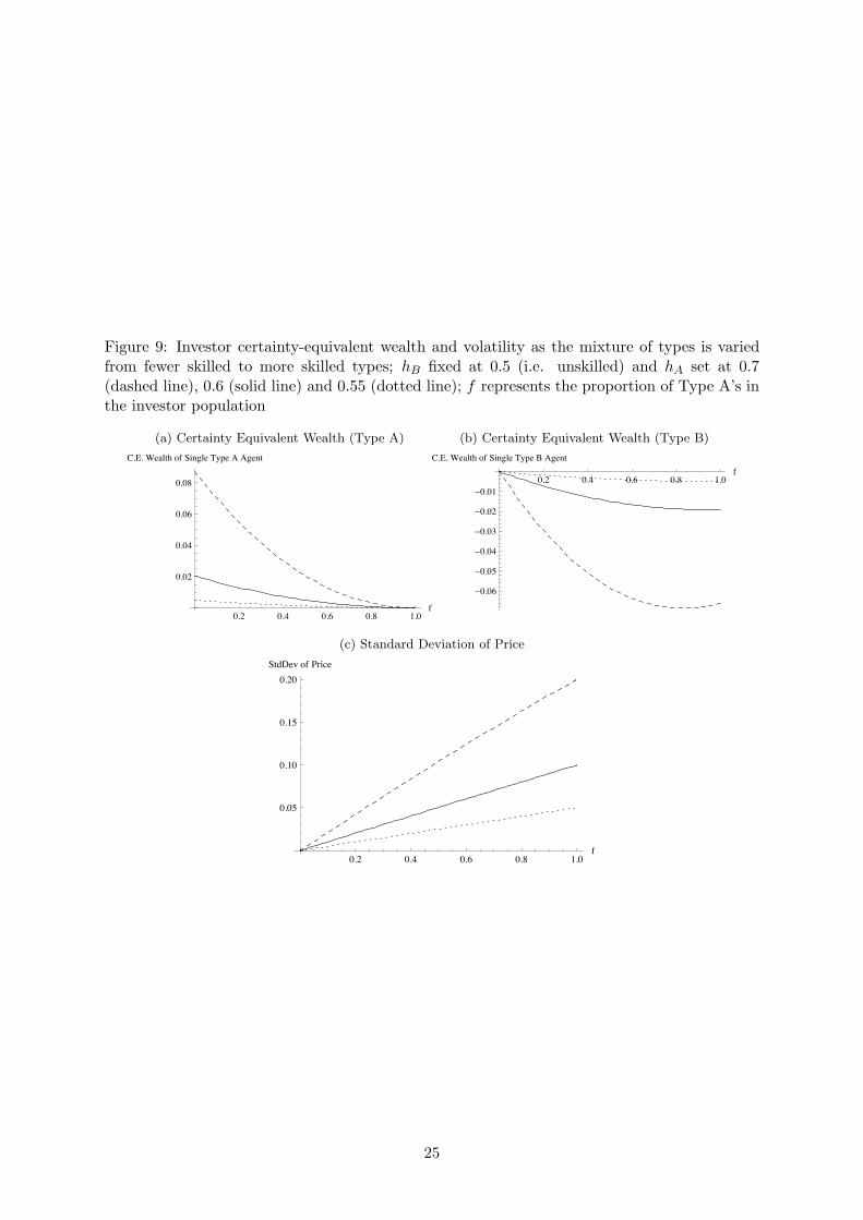
Figure 9: Investor certainty-equivalent wealth and volatility as the mixture of types is variedfrom fewer skilled to more skilled types; hB fixed at 0.5 (i.e. unskilled) and hA set at 0.7(dashed line), 0.6 (solid line) and 0.55 (dotted line); f represents the proportion of Type A’s inthe investor population
(a) Certainty Equivalent Wealth (Type A)
0.2 0.4 0.6 0.8 1.0f
0.02
0.04
0.06
0.08
C.E. Wealth of Single Type A Agent
(b) Certainty Equivalent Wealth (Type B)
0.2 0.4 0.6 0.8 1.0f
!0.06
!0.05
!0.04
!0.03
!0.02
!0.01
C.E. Wealth of Single Type B Agent
(c) Standard Deviation of Price
0.2 0.4 0.6 0.8 1.0f
0.05
0.10
0.15
0.20StdDev of Price
25

Figure 10: Investor certainty-equivalent wealth and volatility as the mixture of types is variedfrom fewer skilled to more skilled; hB fixed at 0.6 and hA set at 0.8 (dashed line), 0.7 (solidline) and 0.65 (dotted line)
(a) Certainty Equivalent Wealth (Type A)
0.2 0.4 0.6 0.8 1.0f
0.05
0.10
0.15
C.E. Wealth of Single Type A Agent
(b) Certainty Equivalent Wealth (Type B)
0.2 0.4 0.6 0.8 1.0f
!0.12
!0.10
!0.08
!0.06
!0.04
!0.02
C.E. Wealth of Single Type B Agent
(c) Standard Deviation of Price
0.2 0.4 0.6 0.8 1.0f
0.05
0.10
0.15
0.20
0.25
0.30StdDev of Price
26
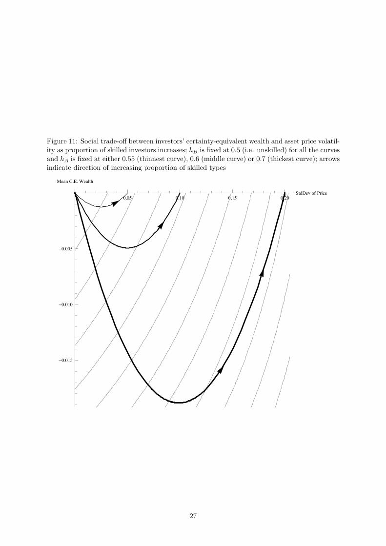
Figure 11: Social trade-o! between investors’ certainty-equivalent wealth and asset price volatil-ity as proportion of skilled investors increases; hB is fixed at 0.5 (i.e. unskilled) for all the curvesand hA is fixed at either 0.55 (thinnest curve), 0.6 (middle curve) or 0.7 (thickest curve); arrowsindicate direction of increasing proportion of skilled types
0.05 0.10 0.15 0.20StdDev of Price
!0.015
!0.010
!0.005
Mean C.E. Wealth
27

Figure 12: Social trade-o! between investors’ wealth and asset price volatility as proportionof skilled investors increases; hB is fixed at 0.6 for all the curves and hA is fixed at either0.65 (thinnest curve), 0.7 (middle curve) or 0.8 (thickest curve); arrows indicate direction ofincreasing proportion of skilled types; point a represents entire population at the lower hit-rate(which is always 0.6), while b, c and d represent entire population at the higher hit-rates (0.65,0.7 and 0.8 respectively)
a b c d0.05 0.10 0.15 0.20 0.25 0.30StdDev of Price
!0.04
!0.03
!0.02
!0.01
Mean C.E. Wealth
28
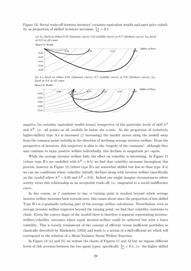
Figure 13: Social trade-o! between investors’ certainty-equivalent wealth and asset price volatil-ity as proportion of skilled investors increases; "A
"B= 0.1.
(a) hA fixed at either 0.55 (thinnest curve), 0.6 (middle curve) or 0.7 (thickest curve); hB fixedat 0.5 in all cases
0.05 0.10 0.15 0.20StdDev of Price
!0.05
!0.04
!0.03
!0.02
!0.01
Mean C.E. Wealth
(b) hA fixed at either 0.65 (thinnest curve), 0.7 (middle curve) or 0.8 (thickest curve); hB
fixed at 0.6 in all cases
0.05 0.10 0.15 0.20 0.25 0.30StdDev of Price
!0.10
!0.08
!0.06
!0.04
!0.02
Mean C.E. Wealth
negative (in certainty equivalent wealth terms) irrespective of the particular levels of skill hA
and hB, i.e. all points on all isoskills lie below the x-axis. As the proportion of (relativelyhigher-skilled) type A’s is increased (f increasing) the market moves along the isoskill awayfrom the common point initially in the direction of declining average investor welfare. From theperspective of investors, this trajectory is akin to the ‘tragedy of the commons’: although theymay continue to enjoy positive welfare individually, this declines in magnitude per capita.
While the average investor welfare falls, the e!ect on volatility is interesting. In Figure 11(where type B’s are unskilled with hB = 0.5) we find that volatility increases throughout thisprocess, however in Figure 12 (where type B’s are somewhat skilled but less so than type A’s)we can see conditions where volatility initially declines along with investor welfare (specificallyon the isoskill where hA = 0.65 and hB = 0.6). Indeed one might imagine circumstances wheresociety views this relationship as an acceptable trade-o!, i.e. tangential to a social indi!erencecurve.
In due course, as f continues to rise, a turning point is reached beyond which averageinvestor welfare increases back towards zero; this comes about since the proportion of less skilledType B’s is a gradually reducing part of the average welfare calculation. Nevertheless, even asaverage investor welfare improves beyond the turning point, we find that volatility continues toclimb. Given the convex shape of the isoskill there is therefore a segment representing investor-welfare/volatility outcomes where equal investor-welfare could be achieved but with a lowervolatility. This is loosely reminiscent of the concept of e"cient versus ine"cient portfolios asclassically described by Markowitz (1952) and leads to a notion of a skill-e"cient set which willcorrespond to the solution of a Mean-Variance Social Welfare Function.
In Figure 13 (a) and (b) we redraw the charts of Figures 11 and 12 but we impose di!erentlevels of risk aversion between the two agent types: specifically "A
"B= 0.1, i.e. the higher skilled
29
type is the less risk-averse of the two. In the notation of Section 3.1 we recall that:
f =$
$ + (1! $)"A"B
and while the ‘weighted’ frequency f determines equilibrium prices and allocations we plotisoskills with weightings given by $. Clearly this e!ects both the shape and level of the isoskillcurves. The e!ect of the di!erential risk-aversion is that f > $ so the skilled types have adisproportionately high impact on pricing (and volatility) compared to their headcount in thepopulation. Hence the mean certainty-equivalent wealth now reaches much lower levels thanunder equal risk aversion since - for a given level of volatility - a greater proportion of thepopulation are in the low-skilled category.
We now apply these tools to our Type II policy questions but find that direct answers areelusive without more specific knowledge of skill levels, market structure and distribution ofwealth across the population.
Although these examples indicate that a ‘first best’ allocation of skill across investors wouldbe our ‘ignorance is bliss’ point, unless society explicitly outlaws the accumulation of investorskill it seems likely that wealth incentives for skill accumulation on an individual basis willpersist (as depicted, for instance, in Figure 9). This means that to a large extent society mayhave to take the location of the prevailing isoskill curve as exogenously given, depending onthe limitations of investors’ own human capital rather than any structural arrangements in theeconomy itself.
We cautiously hypothesize therefore that policy interventions intended to shift the locationof the isoskill are likely to be slow and costly. In contrast, governments may be able to usefaster-acting policy tools to influence the exact location on the isoskill, e.g. supply side measuresaimed at adjusting the structure of the asset management industry, targeted tax incentives toreward specific types of investment, etc..
In a ‘second best’ world, this highlights the need for policy-makers to attempt to establishwhere on the isoskill their economy is located: if on an ‘ine"cient’ segment then there are clearwelfare incentives to reducing the proportion of skilled types ($), thereby reducing volatilitywhile maintaining (or increasing) average investor welfare. However unless the economy canbe immediately relocated to the new ‘e"cient’ point then the challenge here is that a gradualreduction in $ may lead to reduced investor welfare during the transition period: potentiallyan unpopular consequence.
If the economy is on the ‘e"cient’ segment there may be a perfectly socially-acceptabletrade-o! between investor-welfare and volatility; this depends on the precise levels of skill inthe market as well as society’s preferences, for instance we see possible examples in Figures 12and 13(b) but not in Figures 11 or 13(a). It is also possible in this case that an increase in theskilled population ($) may move society onto a higher indi!erence curve.
30
5 Concluding Remarks
To some degree governments have the policy tools to influence the distribution of financial liter-acy, albeit rather crudely. We have put forward general propositions which provide a theoreticalframework to consider the welfare e!ects of such alterations to an economy’s financial literacyprofile, including required conditions for achieving welfare improvements. Specifically, underthe assumption of normally-distributed wealth, we have shown that social benefits will dependpartly on the relationship between each individual’s initial wealth and subsequent (literacy-induced) gains, and partly on the impact which any measures have on volatility of wealth.17
Ideally, policy measures to increase financial literacy should strive for a negative covariance be-tween initial wealth and wealth gains in order to make a positive contribution to social welfare.Nevertheless if these policies have the side-e!ect of increasing volatility in asset markets thentheir overall welfare impact may still be negative and we have provided a theoretical basis toanalyse this trade-o!.
To make our propositions more vivid we demonstrated their applicability to the case of in-vestment forecasting skill, being a particular facet of financial literacy. Although our model waspredicated on simple assumptions we tentatively found that circumstances favouring skill im-provement may be less commonplace than conventionally believed and we were able to demon-strate several scenarios where skill improvement had questionable value. In this context weaddressed two broad policy categories:
Type I policies concern the levels of skill in the population, keeping the distribution constant.Here we would argue that the benefits of universal investor education must be weighed againstthe e!ects which higher levels of skilled trading can have on volatility. Clearly investor educationwhich does not increase skill would be a suboptimal social investment, but even increased skillcombined with greater volatility may have negative welfare implications for society as a wholeas we demonstrated in Section 4. However, given limited resources to improve financial literacyin specific social groups, our general proposition argues that society should focus educationale!orts very much on the poorest, and such programmes may indeed be welfare-enhancing ifappropriately designed to be volatility-neutral (or volatility-reducing).
Type II policies consider the e!ects of the distribution of skill in the market, keeping levelsconstant. In this case we have shown that in appropriate circumstances it can indeed be sociallydesirable to switch investors between skill levels. This might be achieved by - for instance -encouraging broader consumer participation in actively-managed funds (including 130/30 andhedge funds), or by altering the regulatory environment to allow conventional funds greateractive management flexibility (such as the European Union’s UCITS III directive). Neverthelesswe have been careful to demonstrate that the desirability of such measures depends on the initiallevels and distribution of skill in the market. Once again it is perfectly possible for such policiesto have adverse e!ects on volatility and to therefore be self-defeating. We have shown howanalysis of this welfare/volatility trade-o! can be carried-out by using methods analogous tothose of portfolio theory and hence given a theoretical explanation for the quote ‘...having smartguys there almost caused Wall Street to collapse.’
17In the case of non-normal wealth distributions we extend the calculation to include higher moments of wealthand higher derivatives of utility functions but similar intuition applies.
31

Although these results apparently introduce new complexity into policy making, there isgreat scope for helpful empirical modeling of markets along the lines we have described. Inparticular a wealth of analysts’ forecast data is available from which forecasting skill can bemeasured, along with reports of institutional Assets Under Management which give some senseof distribution of investors across levels of skill. The methods we have introduced in this paperenable the debate to benefit from proper quantitative treatment and raise it from the level offolk myths and value judgements.
This leads us to empirical applications. Assuming access to a suitably broad database offorecasts, trading positions and outcomes, our results suggest a variety of testable hypotheses:
(a) Do investors typically operate close to their optimal skill level? (In section 2 we spe-cialised our proposition to the case of normally-distributed wealth to find simple conditions forthe turning point in marginal utility).
(b) Do more complete markets lead to higher skill levels in general? (Our example in section4 hints at this possibility due to more positive ‘tuning’ e!ects).
(c) Do markets segment into separating equilibria of skilled and unskilled types? (This issuggested by the negative marginal utility achieved when all agents increase skill together).
Finally, it is clear that analysis of skill parameters enables society to detect the extremeimplausibility (even impossibility) of fraudulent investment o!erings which are indeed ‘too goodto be true’. Our framework enhances this by providing a setting in which to model the widesocial damage which can be wrought by such schemes. Financial literacy can indeed be anequitable servant as well as a pernicious master.
A Derivations and Proofs
A.1 Proofs
A.1.1 Proposition 2.1
Proof. Agent i has unconditional expected utility given by:
+%,
#%· · ·
+%,
#%u(w(S, z; !))q(S, z; !)dS(1)dS(2) · · · dS(n)dz
Di!erentiating with respect to the agent’s literacy parameter !i gives:
+%,
#%· · ·
+%,
#%uw(w(S, z; !))w!(S, z; !)q(S, z; !)dS(1) · · · dz +
+%,
#%· · ·
+%,
#%u(w(S, z; !))q!(S, z; !)dS(1) · · · dz
= E [uw(w(S, z; !))w!(S, z; !)] + E!u(w(S, z; !)) q!(S,z;!)
q(S,z;!)
"
Since q is a probability density we can think of q!(S,z;!)q(S,z;!) as if it were a score function; from
well-known properties of the score function it therefore follows that
E!
q!(S,z;!)q(S,z;!)
"= 0 (6)
32

A.1.2 Corollary 2.2
Proof. We deploy Stein’s Lemma to rewrite (1) in more familiar terms. This results in acondition for positive marginal utility of literacy as follows:
COV [uw(w), w!] + COV!u(w), q!
q
"+ E [uw(w)] E [w!] > 0
E [uww(w)] COV [w, w!] + E [uw(w)] COV!w, q!
q
"+ E [uw(w)] E [w!] > 0
COV!w, q!
q
"+ E [w!]
COV [w, w!]> RA
where
RA " !E [uww(w)]E [uw(w)]
is the coe"cient of risk aversion defined by Rubinstein (1973).
A.1.3 Proposition 2.3
Proof. For clarity we consider here only the case of discrete types: suppose we have N agenttypes, each with a heterogeneous utility function u[i] and being a proportion f (i) of the pop-ulation. Agent type i has initial (certain) wealth denoted by w(i)
0 and future state-dependentwealth represented by the function w(i)(S, z; !). We assume we have a utilitarian (i.e. equally-weighted) social welfare function. We denote the j’th derivative of u[i] by u[i](j). If agents refrainentirely from investing (i.e. there is no trading with each other) then the value of this welfarefunction is given by
SWF0 =N#1%
i=0
f (i)u(i)(w(i)0 )
However when agents do engage in trade (with a vector of skill parameters !) then ex anteexpected social welfare is given by
SWF (!) =N#1%
i=0
f (i)E[u(i)(w(i)(S, z; !))]
=N#1%
i=0
f (i)E
-
.u(w(i)0 ) +
%%
j=1
1j!
(w(i)(S, z; !)! w(i)0 )ju[i](j)(w(i)
0 )
/
0
= SWF0 +N#1%
i=0
f (i)E
-
.%%
j=1
1j!
(w(i)(S, z; !)! w(i)0 )ju[i](j)(w(i)
0 )
/
0
= SWF0 +%%
j=1
N#1%
i=0
f (i) u[i](j)(w(i)
0 )j!
E*1
#w(i)(S, z; !)2j
+
33

Hence the net welfare e!ect of trading is given by the second term. We call this the SocialBenefit of Trading (SBT ) which is therefore given by:
SBT (!) =%%
j=1
Ef
&u(j)(w0)
j!M (j)(!)
'
where Ef indicates that expectation is taken with respect to the cross-sectional distribution oftypes f and M (j)(!) denotes the j’th moment of the type-specific change in wealth which isequal to E
!##w(i)(S, z; !)
$j".
A.1.4 Proposition 2.6
Proof. Suppose we make a discrete forecast S of either 0 or 1 in respect of a discrete outcomeQ which is also either 0 or 1. We define the following probabilities:
P[S = 1] = g
P[Q = 1|S = 1] = P [Q = 0|S = 0] = h
We list the possible outcomes and joint probabilities of (S,Q) pairs in Table 4 and hence computethe following:
E [SQ] = gh
E [S] = E [Q] = g
V [S] = V [Q] = g(1! g)
COV [S, Q] = gh! g2 = g(h! g)
IC = COR [S, Q] =COV [S, Q]3
V [S] V [Q]=
h! g
1! g
For example when g = 12 we have IC = 2h! 1.
Table 4: Joint distribution of forecast S and actual outcome Q where h denotes hit-rate and gdenotes marginal probability of a forecast equal to 1
S Q SQ P [S, Q]0 0 0 (1! g)h0 1 0 (1! g)(1! h)1 0 0 g(1! h)1 1 1 gh
References
Agenor, P.-R. and J. Aizenman (1999): “Volatility and the welfare costs of financialmarket integration,” in The Asian financial crisis: causes, contagion and consequences,ed. by P.-R. Agenor, M. Miller, D. Vines, and A. Weber, Cambridge University Press.
Aghion, P. and A. Banerjee (2005): Volatility and Growth, Oxford University Press.
34

Aragon, G. and W. Ferson (2006): “Portfolio Performance Evaluation,” Foundationsand Trends in Finance, 2, 83–190.
Bachelier, L. (1900): “Theory of Speculation,” in The Random Character of Stock Mar-ket Prices, ed. by P. Cootner, MIT Press, 17–78.
Bain, W. (1996): Investment Performance Measurement, Woodhead Publishing.
Basak, S. (1997): “Consumption choice and asset pricing with a non-price-taking agent,”Economic Theory, 10, 437–462.
Caballero, R. (2000): “Aggregate Volatility in Modern Latin America: Causes andCures,” MIT Department of Economics Working Paper No 00-11.
Campbell, J. Y. and A. S. Kyle (1988): “Smart Money, Noise Trading and StockPrice Behavior,” NBER Technical Working Papers 0071, National Bureau of EconomicResearch, Inc.
Chaganty, N. and H. Joe (2006): “Range of correlation matrices for dependentBernoulli random variables,” Biometrika, 93, 197–206.
Coggin, T. and J. Hunter (1983): “Problems in Measuring the Quality of InvestmentInformation: The Perils of the Information Coe"cient,” Financial Analysts Journal.
Cox, C. (2006): “Improving Financial Literacy in the United States,” Testimony beforethe U.S. Senate Committee on Banking, Housing and Urban A!airs (May 23rd).
DeLong, J. B., A. Shleifer, L. Summers, and R. Waldmann (1990): “Noise TraderRisk in Financial Markets,” Journal of Political Economy, 98, 703–738.
Detemple, J. and S. Murthy (1994): “Intertemporal Asset Pricing with HeterogeneousBeliefs,” Journal of Economic Theory, 62, 294–320.
Dimson, E. and P. Marsh (1984): “An Analysis of Brokers’ and Analysts’ UnpublishedForecasts of UK Stock Returns,” Journal of Finance, 39, 1257–1292.
EBF (2009): “EBF Report on Financial Literacy,” European Banking Federation (19thMay 2009).
Emmerson, C. and M. Wakefield (2003): “Achieving Simplicity, Security and Choice inRetirement? An Assessment of the Government’s Proposed Pension Reforms,” BriefingNote 36, IFS London.
Fabozzi, F., S. Focardi, and C. Jonas (2008): “Challenges in Quantitative EquityManagement,” Research Foundation of CFA Institute.
Fama, E. (1965): “The Behavior of Stock-Market Prices,” Journal of Business, 38, 34–105.
Fay, S. (1997): The Collapse of Barings, W.W. Norton.
Fishwick, E. (2007): “The information horizon - optimal holding period, strategy aggres-sion and model combination in a multi-horizon framework,” in Forecasting ExpectedReturns in the Financial Markets, ed. by S.Satchell, Academic Press, chap. 10, 215–226.
Frame, D. (1957): The Complete Essays of Montaigne, Stanford University Press.
35

FSA (2005): “Wider-range Retail Investment Products,” FSA Discussion Paper 05/3.
Graham, B. and D. Dodd (1934): Security Analysis, McGraw-Hill.
Granger, C. and M. Machina (2006): “Forecasting and Decision Theory,” in Handbookof Economic Forecasting, ed. by G. Elliott, C. Granger, and A. Timmermann, North-Holland.
Grinold, R. and R. Kahn (1999): Active Portfolio Management, McGraw Hill, seconded.
Grossman, S. and J. Stiglitz (1980): “On the Impossibility of Informationally E"cientMarkets,” American Economic Review, 70, 393–408.
Haq, M. U., I. Kaul, and I. Grunberg (1996): The Tobin tax: coping with financialvolatility, Oxford University Press.
He, H. and N. Pearson (1991): “Consumption and portfolio policies with incompletemarkets and short-sale constraints: The infinite dimensional case,” Journal of EconomicTheory, 54.
Herold, U. (2003): “Portfolio Construction with Qualitative Forecasts,” Journal of Port-folio Management, 30, 61–72.
Hung, A., A. Parker, and J. Yoong (2009): “Defining and Measuring Financial Lit-eracy,” Rand Corporation Working Paper WR-708.
Kahneman, D. and A. Tversky (1979): “Prospect Theory: An Analysis of Decisionunder Risk,” Econometrica, 47, 263–291.
Knight, J. and S. Satchell (2002): Performance Measurement in Finance,Butterworth-Heinemann.
Lee, W. (2000): Theory and Methodology of Tactical Asset Allocation, Wiley.
Leland, H. (1999): “Beyond Mean-Variance: Performance Measurement in a Nonsym-metrical World,” Financial Analysts Journal, 27–36.
Lintner, J. (1969): “The Aggregation of Investors’ Diverse Judgements and Preferences inPurely Competitive Security Markets,” Journal of Financial and Quantitative Analysis,4, 347–400.
Lowenstein, R. (2001): When Genius Failed: The Rise and Fall of Long-Term CapitalManagement, Random House.
Lusardi, A. (2008): “Financial Literacy: An Essential Tool for InformedConsumer Choice?” http://www.dartmouth.edu/~alusardi/Papers/Lusardi_
Informed_Consumer.pdf.
Malkiel, B. G. (1973): A Random Walk Down Wall Street, W.W. Norton and Co.
Markopolos, H. (2010): No One Would Listen: A True Financial Thriller, Wiley.
Markowitz, H. (1952): “Portfolio Selection,” Journal of Finance, 7, 77–91.
Mas-Colell, A., M. Whinston, and J. Green (1995): Microeconomic Theory, OxfordUniversity Press.
36

Obama, B. (2010): “Remarks by the President on Financial Reform,”Http://www.whitehouse.gov/the-press-o"ce/remarks-president-financial-reform.
Perotti, E. (1995): “Credible Privatization,” American Economic Review, 85, 847–859.
Rubinstein, M. (1973): “A Comparative Statics Analysis of Risk Premiums,” Journal ofBusiness, 46, 605–615.
Satchell, S. and O. Williams (2007): “Optimal Forecasting Horizon for Skilled In-vestors,” in Forecasting Expected Returns in the Financial Markets, ed. by S. Satchell,Academic Press.
——— (2010): “On the di"culty of measuring forecasting skill in financial markets,”Unpublished.
Shleifer, A. (1999): Ine"cient markets: An introduction to behavioral finance, OxfordUniversity Press.
Simon, H. (1987): “Rationality in Psychology and Economics,” in Rational Choice, ed. byR.Hogarth and M.Reder, University of Chicago Press, 25–40.
Tajar, A., M. Denuit, and P. Lambert (2001): “Copula-type representation for ran-dom couples with Bernoulli margins,” University Catholique de Louvain Institut DeStatistique Discussion Paper 118.
Treasury, H. M. (2009): “Reforming financial markets,” CM 7667.
Trillin, C. (2009): “Wall Street Smarts,” The New York Times (14th October 2009).
van Rooij, M., A. Lusardi, and R. Alessie (2007): “Financial Literacy and StockMarket Participation,” http://www.dartmouth.edu/~alusardi/Papers/Literacy_
StockMarket.pdf.
Vila, J.-L. and T. Zariphopoulou (1997): “Optimal Consumption and Portfolio Choicewith Borrowing Constraints,” Journal of Economic Theory, 77, 402–431.
Williams, O. (2009): “Asset Pricing With Heterogeneous Skilled Agents,” PhD Disser-tation, University of Cambridge Faculty of Economics.
Zapatero, F. (1998): “E!ects of Financial Innovations on Market Volatility when Beliefsare Heterogeneous,” Journal of Economic Dynamics and Control, 22, 597–626.
37