Social Networks, Ethnicity, and Entrepreneurship

William R. Kerr Martin Mandorff

Working Paper 16-042

Working Paper 16-042

Copyright © 2015, 2016 by William R. Kerr and Martin Mandorff

Working papers are in draft form. This working paper is distributed for purposes of comment and discussion only. It may not be reproduced without permission of the copyright holder. Copies of working papers are available from the author.

Social Networks, Ethnicity, and Entrepreneurship

William R. Kerr Harvard Business School

Martin Mandorff Swedish Competition Authority

Social Networks, Ethnicity, and Entrepreneurship

William R. KerrHarvard University and NBER

Martin Mandorff∗

Swedish Competition Authority

June 14, 2016

Abstract

We study the relationship between ethnicity, occupational choice, and entre-preneurship. Immigrant groups in the United States cluster in specific businesssectors. For example, the concentration of Korean self-employment in dry clean-ers is 34 times greater than other immigrant groups, and Gujarati-speaking Indi-ans are similarly 108 times more concentrated in managing motels. We developa model of social interactions where non-work relationships facilitate the acquisi-tion of sector-specific skills. The resulting scale economies generate occupationalstratification along ethnic lines, consistent with the reoccurring phenomenon ofsmall, socially-isolated groups achieving considerable economic success via con-centrated entrepreneurship. Empirical evidence from the United States supportsour model’s underlying mechanisms.

Key words: entrepreneurship, self-employed, occupation, ethnicity, immigration,networks.

JEL codes: L26; D21, D22, D85, F22, J15, L14, M13.

∗Comments are appreciated and can be sent to wkerr@hbs.edu. We thank Gary Becker, OlaBengtsson, Gustaf Bruze, Dennis Carlton, Barry Chiswick, Rob Fairlie, Matthew Gentzkow, EmilIantchev, Svante Janson, Mini Kaur, Steven Lalley, Ben Mathew, Andriy Protsyk, Jesse Shapiro,Rachel Soloveichik, Chad Syverson, Robert Topel and Nick Wormald and seminar participants forvery valuable comments. We thank Meir Brooks and Rahul Gupta for excellent research support.The theory section of this paper draws heavily from Mandorff’s Ph.D. Dissertation at the Universityof Chicago. Financial support from the Marcus Wallenberg Foundation, the Jan Wallander and TomHedelius Foundation, the Esther and T.W. Schultz Dissertation Fellowship, the Markovitz DissertationFellowship, the Kauffman Foundation, and Harvard Business School is gratefully acknowledged.

1

1 Introduction

Minority immigrant groups are more engaged in self-employed entrepreneurship thannatives, especially among newer cohorts of arrivals. Using the 2007-2011 Current Pop-ulation Surveys, Fairlie and Lofstrom (2013) calculate that immigrants represent 25%of new US business owners compared to their 15% workforce share. Moreover, busi-ness owners for a given immigrant ethnic group tend to specialize in a few industries,and these industry choices can vary across ethnic groups. Prominent recent exam-ples from the United States include Korean dry cleaners, Vietnamese nail care salons,Yemeni grocery stores, and Punjabi Indian convenience stores. This is not just a re-cent phenomenon, with prominent examples of earlier ethnic specializations includingJewish merchants in medieval Europe and Chinese launderers in early twentieth cen-tury California. Despite the potential importance of these patterns economically– forexample, The Economist (2016) reports that one-third of all US motels are owned byGujarati Indians– very few studies have examined the origin or consequences of thisethnic specialization for self-employment in detail.We focus on the roles that ethnic group size and isolated social interactions among

group members can have for yielding this entrepreneurial specialization. We developa simple model that considers a small industry where self-employed entrepreneurs canbenefit from social interactions outside of work (e.g., family gatherings, religious andcultural functions, meetings with friends). At these social events, self-employed entre-preneurs have the opportunity to discuss recent customer trends, share best practices,coordinate activities, and so on. The model describes how a small ethnic minoritygroup that has restricted social interactions can have a comparative advantage for self-employment, similar to the account of Chung and Kalnins (2006) for better resourceaccess through ethnic networks in the case of Gujarati hotel owners. We then analyzethe model’s predictions using Census Bureau data for the United States in 2000. Weshow how the size of groups and their social isolation, which we measure using in-marriage rates, strongly predict industrial concentration for immigrant self-employedentrepreneurs. A 10% decline in group size raises the group’s industry concentrationfor self-employment by 6%, and a 10% increase in group isolation boosts concentrationby 5%. We show that these results are robust under many specification variants andusing instrument variable techniques outlined below.We focus on these rationales, ethnic group size and social isolation, for two rea-

sons. The first is the exceptionally broad and pervasive nature of minority immigrantconcentration for self-employment. Kuznets (1960) observes that "all minorities arecharacterized, at a given time, by an occupational structure distinctly narrower thanthat of the total population and the majority." While the particulars vary across eth-nic groups, time periods and national settings, the consistent empirical observation istowards self-employed specialization among ethnic groups that are socially cohesive.

2

Thus, to make progress towards the general pattern, we seek to investigate a generalmechanism that does not revolve around the traits of any single ethnic group or set-ting; similarly, our empirical analysis includes as many immigrant groups in the UnitedStates as possible. Understanding how group-level behavior can generate group-leveldifferences is important, especially as we know that controlling for differences in de-mographic characteristics and other quantifiable attributes does not explain the ethnicentrepreneurship premium.A second rationale is that we believe ethnic group size and group social isolation can

manifest themselves in many ways discussed in the literature. For example, frequentreports comment on how immigrant communities can share risks among members,provide informal support and financial loans, allow for sanctions against misbehavior,and similar. In the context of our study, these factors become more powerful forsmaller, tighter ethnic groups as, for example, a group’s ability to sanction againstpoor behavior depends upon the extent to which the group can punish misdeeds inthe future. Concentrated social ties increase the cost of breaking a contract, addingsocial repercussions to economic and legal penalties. Group influences could also leadto behavioral factors prompting entry into self employment (e.g., Åstebro et al., 2014).We, of course, do not argue that other factors are entirely subordinate to the twothat we emphasize, and data limitations unfortunately do not allow us to horseracetheories. The goal instead is to provide a step towards understanding common traitsthat could be observed in as many settings and with as diverse a set of ethnic groupsas the historical record documents.In advance of our empirical work, we note some important issues. First, while there

are plenty of anecdotal and sociological accounts of how social interactions can con-nect to entrepreneurial activity1, identifying interaction effects is notoriously diffi cult.Unobservable characteristics can give rise to the reflection problem described by Man-ski (1993). Our empirical work could be subject to these concerns of omitted factorsor reverse causality (e.g., self-employment concentration leading to higher in-marriagerates). We consider two instrument variable specifications to address this issue. Oneapproach uses the 1980 group sizes and in-marriage rates in the United States. Oursecond approach instruments US ethnic group size with the predictions from a gravitymodel for migration to the United States and instruments US in-marriage rates withthose observed for the same ethnic group in the United Kingdom. These estimationsconfirm the OLS results. We finally provide earnings estimations consistent with themodel’s predictions.

1For example, Fairlie and Robb (2007) document from the Characteristics of Business Ownersdatabase that more than half of business owners have close relatives who are self-employed, and aquarter of business owners have worked for these relatives. Datasets linking vertically across gener-ations are more common. Dunn and Holtz-Eakin (2000) find that the incidence of self-employment,controlled for other factors, doubles when an individual’s parents are self-employed.

3

Second, we seek to quantify general traits that do not rely on very aggressive defini-tions of industry boundaries, even if this leads us to underestimate some concentration.For example, since people have a proclivity and skill for cuisine from their home coun-try, Greek restaurateurs will sort into Greek restaurants and Chinese restaurateurs willsort into Chinese restaurants, independent of social relationships. This sorting mecha-nism is well-understood and very likely at work in some settings, but we will considerthe restaurant industry as a whole to avoid some of these taste-based factors. Similarly,we will look at industries on a national basis, even though there is clear evidence ofadditional clustering happening at localized levels for some industries (e.g., taxi cabs,landscaping). We use this uniform approach to be consistent over industries, versusfor example defining the motel industry in a different way from taxi cabs, and becauseethnic connections have been measured in parallel settings to provide knowledge andbenefits at extended spatial distances (e.g., Agrawal et al., 2008).Our work connects to several prior literatures. We most directly contribute to stud-

ies of immigrant entrepreneurship and self-employment behavior.2 Compared to manycontributions in this literature, our study focuses much more on quantifying patternsin industrial specialization across groups, versus a detailed study within a single group.As noted earlier, this reflects our goal to build a framework for why the patterns areso consistently observed. In a broader context, we relate to economic and sociolog-ical literatures regarding minority and immigrant group occupational specialization.3

In addition, our setting resembles but differs substantially from the standard theoryof discrimination. We analyze environments when groups are economically integratedbut culturally isolated, in contrast to the Becker (1957) framework where discrimi-nation taxes the market transactions between groups. These important differencesshape whether the minority group isolation can provide a comparative advantage forself-employment or not.4 We also relate to a literature on the importance of socialinteractions for economic behavior outside of the workplace or within it.5

2Important examples include Chung and Kalnins (2006), Fairlie (2008), Gil and Hartman (2009),Fairlie et al. (2010), Jackson and Schneider (2011), Patel and Vella (2013), and Kerr and Kerr (2015).Fairlie and Lofstrom (2013) provide a complete review.

3Related and classic work includes Morris (1956), Winder (1962), Blalock (1967), Milgram (1967),Light (1977), Thernstrom (1980), Landa (1981), Sowell (1981), Aldrich andWaldinger (1990), Milgromet al. (1990), Melton (1990), Sowell (1996), Cohen (1997), Greif (1993), Greif et al. (1994), andBotticini and Eckstein (2005). Our theory is also related to the concept of ethnic capital (Borjas1992, 1995) and group assimilation (Lazear 1999).

4To illustrate how market interaction can take place without social interaction, consider a scenefrom Shakespeare’s The Merchant of Venice (Act 1, Scene III) depicting the social divide between theChristians and Jews in Renaissance Europe. Following a negotiation over a large loan to a Christianman who has always scorned him, the Jewish moneylender Shylock comments: "I will buy with you,sell with you, talk with you, walk with you, and so following; but I will not eat with you, drink withyou, nor pray with you."

5Important examples include Granovetter (1973), Montgomery (1991), Glaeser et al. (1996),

4

Classic accounts of the nature of entrepreneurship emphasize in equal measure dis-ruptive forces that entrepreneurs generate (Schumpeter, 1942, 1988) and their role inreducing price gaps and arbitrage opportunities (Kirzner, 1972, 1979). These theoriesrarely provide specific pressures or predictions for one group to become an entrepreneurversus another, except along defined traits like ability to navigate uncertainty (Knight,1921), risk tolerance (Kihlstrom and Laffont, 1979), business acumen (Lucas, 1978),and skill mix (Lazear, 2005). Connections of entrepreneurship to migration status havebeen frequently noted but poorly explained. A central emphasis in this paper is thatsocial interactions can generate group-level effects towards self-employed entrepreneur-ship and industry choice that are important for explaining why, today and in timespast, some populations show a greater tendency to self-employment, above and be-yond other features that promote entry decisions. Further research needs to continuebuilding out these connections from social networks and occupational structures toentrepreneurship given the general applicability of these phenomena to many ethnicgroups and their persistent roles in many cultures and economies.These findings are also of managerial relevance and policy importance. For immi-

grant entrepreneurs, our work quantifies economic relationships that are often perceivedbut anecdotal. We provide evidence on the power of group choices and also offer in-sights on their long-term stability. For example, new immigrant arrivals to a rapidlyassimilating immigrant group should discount some of the comparative advantage thatis presently visible for their ethnic group in chosen self-employed industries as theyare unlikely to experience as powerful of a force in the future. Our model also high-lights why members of an ethnic group may have an economic incentive to preserveand encourage social isolation, independent of cultural or religious factors. On the flipside, our work provides insights into industry dynamics for other market participants.Business owners in a self-employment industry can forecast increased competition iftheir industry has a very cohesive and socially isolated ethnic group that is set to growrapidly over the next decade, especially if the size of their industry is well matched tothe size of ethnic group. Policy makers can also utilize the results of this study. Studiesof immigration tend to focus on broad employment and wage effects for natives by skilllevel, geographic region, etc. Our study provides insights on how available data can beused to provide more precise industry-level perspectives, differentiated by wage work-ers versus self-employed entrepreneurs, on the likely economic impacts of an immigrantgroup expanding.

Bertrand et al. (2000), Glaeser and Scheinkman (2002), and Calvo-Armengol and Jackson (2004).Durlauf and Fafchamps (2006) and Durlauf and Ioannides (2010) provide broad reviews.

5

2 A Model of Entrepreneurial Clustering

This section develops a simple model to illustrate how social isolation and small groupsize can generate ethnic entrepreneurial clustering when social interactions and produc-tion are complementary. To keep the model tractable and intuitive, we make severalstrong assumptions. First, we consider a setting where everyone has equal innate abil-ity and is divided into two ethnic groups, A and B. Group A is in the minority, with acontinuum of individuals of total mass NA, and group B is the majority, with a contin-uum of individuals of total mass NB > NA. To focus the model on production-relatedcomplementarities, both groups have equal access to industries and there is no productmarket discrimination. We discuss below settings with more than two ethnic groups.While members of groups A and B interact equally in the marketplace, we make a

second assumption that they are socially segregated and spend their leisure time sep-arately. Moreover, we model that social interaction is random within ethnic groups–that is, each person interacts with a representative sample of individuals in their owngroup only.6 Our online appendix analyzes several settings with endogenous socialinteractions, marriage markets, and so forth, finding a large range of conditions underwhich the results developed with random matching hold in more complicated environ-ments.We analyze how these ethnic groups sort across two industries. One industry (which

we label industry 1) is characterized by a production structure where self-employed en-trepreneurs can obtain advantages through social interactions with other self-employedentrepreneurs in the same industry. The production structure in the other industry(which we label industry 0), by contrast, is assumed to have constant returns to scalewith worker productivity normalized to one. Thus, we are assuming that private socialinteractions do not have the same benefit in this industry as they did in industry 1, andthis industry could be equally comprised of individuals working in self-employment orin larger firms.This stark industrial structure serves to isolate in industry 1 a setting where self-

employed entrepreneurs need to rely on their own judgment when they make businessdecisions. When socializing during family gatherings and religious/cultural functions,entrepreneurs in this industry could mentor each other and exchange industry knowl-edge and professional advice. The more an entrepreneur socializes with other entre-preneurs, the more knowledge is exchanged. We are thus explicitly creating a situationwhere social interaction and production are complementary in ways that the otherindustry does not possess (or possesses in very negligible degrees). We return to thisbelow.

6The terms "representative sample" and "random sample" are used interchangeably. They coincideconceptually if the random sample is large enough, which is assumed to be the case.

6

More formally, define Xl for l ∈ {A,B} as the fraction of the population in group lwho are self-employed entrepreneurs in industry 1. We will also refer to this fraction asthe group’s degree of specialization. Since social interaction is random within groups, afractionXl of the friends and family members of every individual in group l are also self-employed entrepreneurs in industry 1. Denote individual entrepreneurial productivityin group l for industry 1 as θ (Xl) . Our initial assumption that productivity increaseswhen socializing with other entrepreneurs in industry 1 is formally stated as:

Assumption 1a Entrepreneurial productivity in industry 1 increases inspecialization: θ′ > 0.

Let us denote the aggregate output of industry 1 as Q1, which is a function of thedistribution (XA, XB):

Q1 (XA, XB) = XANAθ (XA) +XBNBθ (XB) . (1)

Since social interaction is assumed to play no productive role for industry 0, the ag-gregate output of industry 0 is simply:

Q0 (XA, XB) = (1−XA)NA + (1−XB)NB. (2)

Moving to demand, the two industries need to be complementary enough to avoid thecomplications of multiple optima possibly generated by non-convexities. To simplify theexposition, let them be perfect complements. Consumers then have Leontief preferenceswith the utility function:

U (q0, q1) = min(q0,

q1v

), (3)

where v > 0 is a preference parameter and q0 and q1 are individual consumption ofeach industry’s output, respectively.

2.1 The Pareto Problem

We now describe the effi cient outcome; the competitive outcome is described in theonline appendix. Since the outputs of both industries have unitary income elasticities,distributional aspects can be ignored when characterizing the effi cient outcome. Theproblem simplifies to choosing an industry distribution (XA, XB) that maximizes arepresentative utility function U (Q0 (XA, XB) , Q1 (XA, XB)). A marginal analysis isinappropriate since this is a non-convex optimization problem. We consider instead themost specialized industry distributions, where either as many individuals as possible ingroup A or as many individuals as possible in group B are self-employed entrepreneursin industry 1.

7

Figure 1 depicts the production possibilities for the two most specialized distribu-tions. Define V (XA, XB) ≡ Q1

Q0as the ratio of industry outputs under the distribution

(XA, XB). Along the curve with the kink V (1, 0) in the figure, group A specializes asself-employed entrepreneurs in industry 1. Starting from a position on the far rightwhere everyone works in industry 0, members of group A are added to the set of self-employed entrepreneurs in industry 1 as we move leftward along the x-axis. Whenreaching the kink V (1, 0), all members of group A are self-employed entrepreneurs inindustry 1. Thereafter, continuing to move leftward, members of group B are alsoadded to industry 1 until reaching Q0 = 0. Similarly, along the curve with the kinkV (0, 1), group B first specializes as self-employed entrepreneurs in industry 1. Mem-bers of group B are added moving leftward along the x-axis until reaching the kinkV (0, 1), where all Bs are working in industry 1. Thereafter also members of group Aare added until reaching Q0 = 0.The curve with minority specialization is above the curve with majority specializa-

tion, so long as the need for self-employed entrepreneurs in industry 1 is suffi cientlysmall. A large fraction of As are self-employed entrepreneurs in industry 1 when theminority specializes, allowing minority entrepreneurs to socialize mostly with otherentrepreneurs in industry 1, greatly improving productivity. The same is not true forthe majority when they specialize, since even if a large fraction of self-employed entre-preneurs in industry 1 are Bs, most Bs are nevertheless employed in industry 0. As aresult, social interactions do not aid the self-employed entrepreneurs in industry 1 inthis scenario very much.The argument can be generalized to show that minority specialization is Pareto

effi cient so long as industry 1 is small enough. Perfect complementarity simplifies theproblem of solving for the optimal allocation, since any bundle where industrial outputsare in the exact ratio v of the Leontief preferences (3) is strictly preferable to all otherbundles that do not include at least as much of each industry. The Pareto optimaldistribution (XA, XB) must therefore satisfy v = V (XA, XB). Define the total numberof entrepreneurs in the population as M ≡ XANA +XBNB. It follows that:

Proposition 1 If v ≤ V (1, 0), all self-employed entrepreneurs in industry 1 belongto minority group A.

Consequently, the effi cient outcome requires that a single group specializes as self-employed entrepreneurs in industry 1, and importantly, which group specializes is notarbitrary. Minority specialization is more effi cient since the minority’s social isolationenables entrepreneurs in A to socialize mostly within their own isolated group. Propo-sition 1 implies that, for v ≤ V (1, 0), the transformation curve and the curve withminority specialization in Figure 1 coincide. Group A has absolute and comparativeadvantages as self-employed entrepreneurs in industry 1. If the demand for industry

8

1 is suffi ciently great, however, then the minority is too small to satisfy demand bythemselves. In the special case when v = V (0, 1), the demand for industry 1 is greatenough for group B to specialize completely. In this case minority involvement wouldjust serve to dilute the majority’s productivity advantage, and the Pareto effi cientsolution is for Bs to specialize in being self-employed entrepreneurs in industry 1.

Corollary If v = V (0, 1), all self-employed entrepreneurs in industry 1 belong to themajority, B.

As the corollary shows, the relationship between group size and productivity is notmonotonic. Rather, the group with the absolute advantage is the group with a popu-lation size that most closely adheres to the size of industry 1 where social interactionand production are complementary. Other production possibilities generated by moreunspecialized distributions, such as XA = XB, are not displayed in Figure 1. Sincesome of these production plans could be above the two specialized curves in Figure 1,the transformation frontier cannot be fully characterized at this stage. The productionfunction must be restricted further to allow a complete characterization.

2.2 Quality and Convex Productivity

In addition to the quantity of social interactions with other self-employed entrepreneurs,the quality of these interactions could also matter for productivity. Let individualproductivity for self-employed entrepreneurs in industry 1 increase both in the quantityand average productivity of other entrepreneurs in the sector of the same group. Writethis as

θ = φ+ δXlθ, (4)

where φ > 0 is a productivity term, 0 < δ < 1 is a social multiplier, Xl is the fractionof entrepreneurs in group l, and θ is the average productivity of these entrepreneurs.Solving for equilibrium productivity by setting θ equal to θ, individual productivity ingroup l is a function:

θ (Xl) =φ

1− δXl

. (5)

Under these conditions, productivity is convex in the degree of specialization whentaking both the quantity and the quality of interaction into account.7 With this resultin mind, we make the following assumption:

7This specification highlights the differences from a standard interaction model. The standardmodel is generally specified so that individual productivity is a function of a group-specific term φ

and the discounted mean of the group, δθ. Solving θ = φ+ δθ, interaction exacerbates the differencein φ across groups, θ = φ

1−δ > φ, but the degree of specialization Xl has no effect on productivity.

9

Assumption 1B Productivity of self-employed entrepreneurs in industry 1 is convexin specialization: θ′′ > 0.

Assumption 1B allows a full characterization of the effi cient solution without havingto resort to explicit functional form. It is further discussed in the online appendix, anda full model is provided that does not require this condition. Convex productivity givesthe following result:

Lemma If productivity is convex, both groups never work in both industries.

The effi cient economy aims for maximum ethnic homogeneity in self-employed en-trepreneurship in industry 1. Ruling out that both groups work in both sectors impliesthat only the specialized distributions along the two curves depicted in Figure 1 couldpossibly coincide with the transformation frontier. The shape of the entire transforma-tion frontier can therefore be deduced by tracing out the maximum of the two curvesin that figure.

Proposition 2 If productivity is convex, there is a cutoff value v∗ such that forv < v∗, the minority group specializes as self-employed entrepreneurs in industry 1,whereas for v > v∗, the majority specializes.

Figure 2 shows how the degree of specialization varies with the size of industry 1, asgoverned by v, and the cutoff value v∗ for majority group specialization. The greaterthe value of v, the greater is the demand for industry 1 and the more people work init. As industry 1 increases in size in Figure 2, the interaction externality generates acharacteristic discrete jump from one type of equilibrium to another. At the point v∗,where many from group B have also joined self-employed entrepreneurship in industry1, the economy abruptly moves from minority specialization to majority specialization.

2.3 Model Discussion

This simple model provides a stark economic environment for considering how isolatedsocial interactions could impact the sorting of ethnic groups over industries. We have,of course, only modelled two industries, while the world has many. This simplificationis not as limiting as it may first appear. The model is simply trying to capture a settingwhere a small industry of self-employed entrepreneurs can benefit through non-workinteractions. Allowing the baseline industry 0 in the framework, which has constantproductivity and non-returns to interactions, to be broken up into many industrieswould not overturn the result that the effi cient solution is for the small ethnic groupto specialize in being the self-employed entrepreneurs if their group size matches thedemand preferences for industry 1. In fact, framed this way, the baseline industry 0

10

would be expected to be quite large to any one industry, making it more likely thatthe minority group should specialize.Another obvious simplification is that we only have two ethnic groups, whereas

the world is much more diverse. Yet, a complex model allowing for several smallindustries and also several minority ethnic groups would lead to the same conclusions.For example, consider an economy with industries 1a and 1b that have equal demandand display the same productivity benefit for social interaction. Also allow there tobe two minority groups of equal size. If the demands for industries 1a and 1b aresuffi ciently small, then the effi cient outcome is for one minority group to specialize inbeing self-employed entrepreneurs in 1a, and for the other minority group to specializein 1b. Which minority group specializes in which sector is arbitrary. In this multi-sectoreconomy with sector-specific skills, otherwise-similar groups consequently specialize indifferent business sectors. Pushing further, if the economy has several small industriesof varying sizes that benefit from these social interactions, and multiple minority ethnicgroups, the effi cient outcome will be characterized by minority groups specializing inspecific self-employment industries as much as possible.The online appendix provides an extended analysis of this model, including analy-

sis of competitive outcomes; occupational stratification and the dynamics of groupspecialization; individual heterogeneity in ability and earnings; marriage markets; andthe formation of splinter groups. Perhaps the most important extension is into earn-ings, where the extended model predicts that members of an ethnic group can achievegreater earnings when entering a common self-employed industrial specialization. Thisis important for separating the positive social complementarities rationale for minorityspecialization from classic discrimination accounts.8 Our upcoming empirical analysisfocuses exclusively on the group size, social isolation, and self-employed entrepreneurialclustering relationships articulated in the simple model, and we hope future researchconsiders more of the additional predictions made in the extended model.

3 Analysis of US Entrepreneurial Stratification

This section assesses the extent to which the social isolation and small group sizes ofethnic immigrant communities lead to entrepreneurial stratification. We begin witha description of our US 2000 Census of Populations sample and our metrics for cal-

8The empirical work of Patel and Vella (2013) strongly shows a positive earning relationship forimmigrant groups and common group occupational choices, and the appendix also provides somecomplementary evidence from our own data. The favorable economic outcome does not necessarilycarry over to utility. Depending on the degree of endogeneity of social interaction, the overall situationfor minority groups may still be worse than the overall situation for the majority. Related work alsoincludes Chiswick (1978), Borjas (1987), Simon and Warner (1992), Rauch (2001), Mandorff (2007),Bayer et al. (2008), and Beaman (2012).

11

culating entrepreneurial clustering and social isolation. Our initial analysis includesdescriptive measures of prominent ethnic entrepreneurship groups and OLS regressionsof our ethnic concentration ratios on ethnic group size and isolation. We then addressendogeneity concerns using a two-stage least squares instrumental variable (IV) ap-proach. We corroborate evidence through a series of robustness checks, including asimulation methodology that verifies our entrepreneurial cluster measures are robustto controls for small ethnic group sizes. We close with a discussion of earnings.

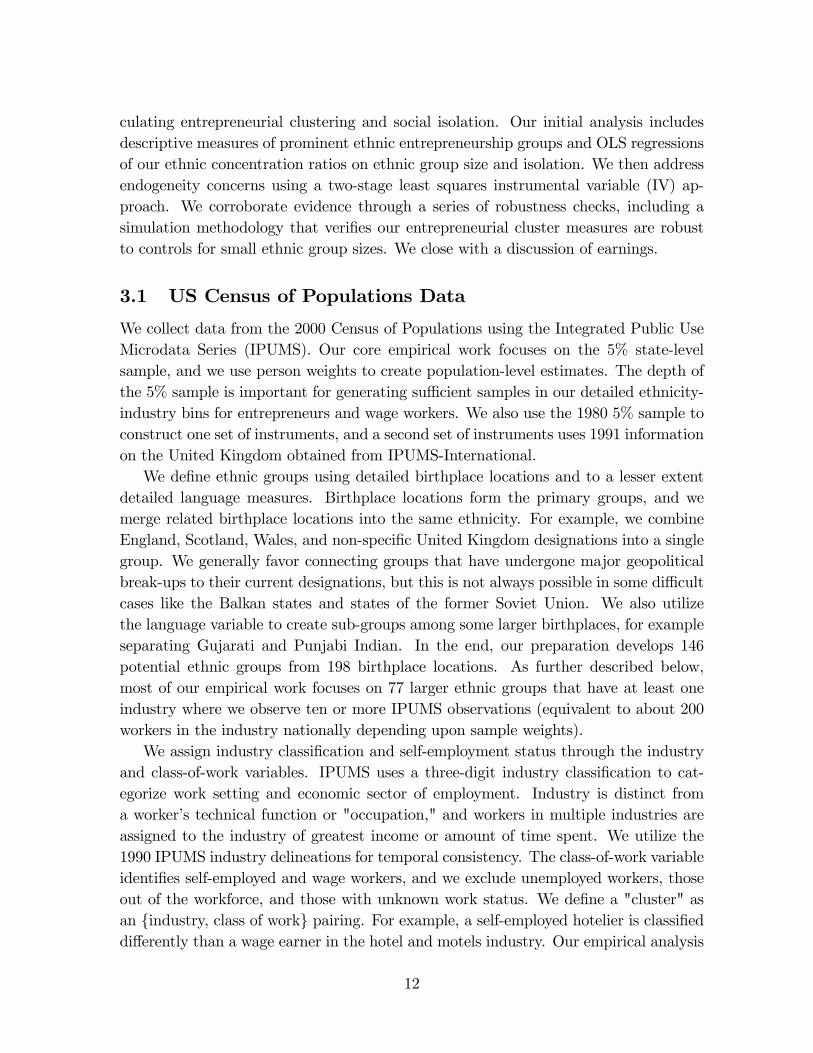
3.1 US Census of Populations Data

We collect data from the 2000 Census of Populations using the Integrated Public UseMicrodata Series (IPUMS). Our core empirical work focuses on the 5% state-levelsample, and we use person weights to create population-level estimates. The depth ofthe 5% sample is important for generating suffi cient samples in our detailed ethnicity-industry bins for entrepreneurs and wage workers. We also use the 1980 5% sample toconstruct one set of instruments, and a second set of instruments uses 1991 informationon the United Kingdom obtained from IPUMS-International.We define ethnic groups using detailed birthplace locations and to a lesser extent

detailed language measures. Birthplace locations form the primary groups, and wemerge related birthplace locations into the same ethnicity. For example, we combineEngland, Scotland, Wales, and non-specific United Kingdom designations into a singlegroup. We generally favor connecting groups that have undergone major geopoliticalbreak-ups to their current designations, but this is not always possible in some diffi cultcases like the Balkan states and states of the former Soviet Union. We also utilizethe language variable to create sub-groups among some larger birthplaces, for exampleseparating Gujarati and Punjabi Indian. In the end, our preparation develops 146potential ethnic groups from 198 birthplace locations. As further described below,most of our empirical work focuses on 77 larger ethnic groups that have at least oneindustry where we observe ten or more IPUMS observations (equivalent to about 200workers in the industry nationally depending upon sample weights).We assign industry classification and self-employment status through the industry

and class-of-work variables. IPUMS uses a three-digit industry classification to cat-egorize work setting and economic sector of employment. Industry is distinct froma worker’s technical function or "occupation," and workers in multiple industries areassigned to the industry of greatest income or amount of time spent. We utilize the1990 IPUMS industry delineations for temporal consistency. The class-of-work variableidentifies self-employed and wage workers, and we exclude unemployed workers, thoseout of the workforce, and those with unknown work status. We define a "cluster" asan {industry, class of work} pairing. For example, a self-employed hotelier is classifieddifferently than a wage earner in the hotel and motels industry. Our empirical analysis

12

focuses on self-employment industries, and we consider total industry employment inrobustness checks. We drop observations of 24 industries in which self-employment isnon-existent (e.g., military, railroads, the US postal service, religious organizations).Our final sample includes 200 industries.We narrow our sample using demographic information available in the IPUMS

dataset. For immigrants and US-born workers, we retain males between 30 and 65years old who are living in metropolitan statistical areas.9 We further require thatimmigrants arrived in the United States before 1990 to avoid issues related to migrationfor temporary employment (which in the United States is typically in roles selected bythe sponsoring firm and can last for six years on the H-1B program). To circumventschooling decisions that are influenced by other forms of social interaction than thosediscussed here, we require that immigrants be at least 20 years of age at the time ofimmigration to the United States. Immigrants must also have immigrated no earlierthan 1969.10 Our final sample contains 1,604,350 observations representing 34,984,436people when applying sample weights. Of these individuals, 143,327 observations,representing 3,141,080 people, are immigrants.

3.2 Clustering in Entrepreneurial Activities

We study entrepreneurship through self-employment status. The use of the term "en-trepreneurship" differs greatly across studies, and our focus here is on a broad definitionthat includes both employer firms and sole proprietors. Likewise, our definition cap-tures firms with a full range of growth ambitions and prospects, from independentartisans to high-growth firms supported by venture capital investors. As we considerpopulation-level counts, our definitions are mostly determined through "Main Street"activity like restaurants, barber shops, construction, retail trade, and similar. Be-cause classification is discrete in the class-of-work variable, we tend to only captureself-employment when it is the main activity of an individual (e.g., not capturing aca-demics who consult part-time to companies).The central focus of our theory is on the concentration of ethnic entrepreneurs

in particular industries. We devise "overage" ratios, defined below, to quantify theheightened rate of ethnic self-employment in a particular industry and also across arange of industries. Our core metrics, used in most of our empirical analysis andthe default for the discussion below, only retain individuals that are self-employed,

9Faggio and Silva (2014) analyze differences in self-employment alignment to entrepreneurship inurban and rural areas.10The Immigration and Naturalization Services Act of 1965 abolished national origin restrictions,

allowing large-scale non-European immigration for the first time since the Chinese Exclusion Act of1882. Our sample requires immigration no earlier than 1969 since the Act went into effect in June of1968.

13

considering variation in ethnic groups across industries. In robustness checks we alsocalculate overage ratios on industry total employment, combining wage earners andself-employed workers.11

To define our metrics, we identify each employed worker xi’s ethnic group andindustry. We define OV ERlk as the ratio of an ethnic group l’s concentration in anindustry k to the industry’s national employment share. Thus, if ethnic group l hasNl total workers and Nk

l workers in industry k, then Xkl = Nk

l /Nl and OV ERlk =Xkl /X

k. The subscript lk denotes that these two metrics are unique to each group-industry pairing, and we calculate OV ERlk for each industry where the ethnic groupis employed.To move from these industry-level values to analyses of entrepreneurial group con-

centration, our core estimates take a weighted average across industry-level overagevalues for each ethnic group, with the weights being the share of the group’s self-employment that is present in that industry:

OV ER1l =K∑k=1

OV ERlkXkl . (6)

Our estimations ultimately use the log value of this OV ER1 metric. We also considerseveral variants in robustness checks. One set of robustness checks considers differentsamples for OV ER1l, such as including rural populations or excluding natives from theXk denominators used in OV ERlk. A second approach varies the formula in severalways:

1. Weighted average over the three largest industries for ethnic group l: OV ER2l =∑3k′=1OV ERlk′X

k′l /∑3

k′=1Xk′l , where k

′ = k such that∑3

k′=1Nk′l is maximized.

2. Weighted average over the three largest industry-level overages for ethnic group l:OV ER3l =

∑3k′=1OV ERlk′X

k′l /∑3

k′=1Xk′l , where k

′ = k such that∑3

k′=1OV ERlk′

is maximized.

3. Maximum overage: OV ER4l = maxl[OV ERlk].

In making these calculations that measure extreme values, we need to be carefulabout small sample size. We first require that ethnicities included in our sample have

11It may seem appealing to use wage earners instead as a counterfactual to self-employed workers.This approach, however, does not offer a good counterfactual as ethnic entrepreneurs show a greatertendency to hire members of their own ethnic groups into their firms (e.g., Andersson et al., 2009,2012; Åslund et al., 2012; Kerr et al., 2015). A Yemeni grocery store owner, taking as an exampleour second most concentrated cluster discussed below in Table 1b, is far more likely to hire Yemeniemployees into the growing firm. We thus use this as a robustness check that provides us deepersample sizes.

14

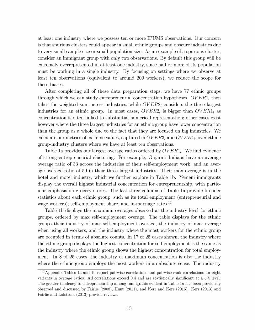
at least one industry where we possess ten or more IPUMS observations. Our concernis that spurious clusters could appear in small ethnic groups and obscure industries dueto very small sample size or small population size. As an example of a spurious cluster,consider an immigrant group with only two observations. By default this group will beextremely overrepresented in at least one industry, since half or more of its populationmust be working in a single industry. By focusing on settings where we observe atleast ten observations (equivalent to around 200 workers), we reduce the scope forthese biases.After completing all of these data preparation steps, we have 77 ethnic groups

through which we can study entrepreneurial concentration hypotheses. OV ER1l thentakes the weighted sum across industries, while OV ER2l considers the three largestindustries for an ethnic group. In most cases, OV ER2l is bigger than OV ER1l asconcentration is often linked to substantial numerical representation; other cases existhowever where the three largest industries for an ethnic group have lower concentrationthan the group as a whole due to the fact that they are focused on big industries. Wecalculate our metrics of extreme values, captured in OV ER3l and OV ER4l, over ethnicgroup-industry clusters where we have at least ten observations.Table 1a provides our largest overage ratios ordered by OV ER1l. We find evidence

of strong entrepreneurial clustering. For example, Gujarati Indians have an averageoverage ratio of 33 across the industries of their self-employment work, and an aver-age overage ratio of 59 in their three largest industries. Their max overage is in thehotel and motel industry, which we further explore in Table 1b. Yemeni immigrantsdisplay the overall highest industrial concentration for entrepreneurship, with partic-ular emphasis on grocery stores. The last three columns of Table 1a provide broaderstatistics about each ethnic group, such as its total employment (entrepreneurial andwage workers), self-employment share, and in-marriage rates.12

Table 1b displays the maximum overages observed at the industry level for ethnicgroups, ordered by max self-employment overage. The table displays for the ethnicgroups their industry of max self-employment overage, the industry of max overagewhen using all workers, and the industry where the most workers for the ethnic groupare occupied in terms of absolute counts. In 17 of 25 cases shown, the industry wherethe ethnic group displays the highest concentration for self-employment is the same asthe industry where the ethnic group shows the highest concentration for total employ-ment. In 8 of 25 cases, the industry of maximum concentration is also the industrywhere the ethnic group employs the most workers in an absolute sense. The industry

12Appendix Tables 1a and 1b report pairwise correlations and pairwise rank correlations for eightvariants in overage ratios. All correlations exceed 0.4 and are statistically significant at a 5% level.The greater tendency to entrepreneurship among immigrants evident in Table 1a has been previouslyobserved and discussed by Fairlie (2008), Hunt (2011), and Kerr and Kerr (2015). Kerr (2013) andFairlie and Lofstrom (2013) provide reviews.

15

size variable ranks industries from largest (1) to smallest (200) in terms of their overallsize in the economy. Most of the maximum-concentration industries in the first twoindustry lists are of moderate size; industries in the third set for highest absolute countof ethnic employees tend to be larger industries.We pause now to reflect on some of the features displayed in these tables. First, it

is noteworthy from viewing the tabulations that some important factors outside of themodel are surely aiding group concentration but are not captured by our theoreticaland empirical work, while still being of a similar spirit in terms of the conceptual ideasof this paper. For example, we treat the taxi industry as a single industry for ourempirical work, but in most respects taxi markets are segmented by cities. Frequenttravelers note the degree to which different ethnic groups appear to dominate thetaxi industry on a city-by-city basis, with the most important group for each citybeing different. In fact, more broadly, many industries of maximum concentration(e.g., grocery stores, gas stations) are cases where geography can play an importantrole. This suggests we are likely under-estimating true concentration in this regard.13

A second, but seemingly smaller, factor from these tables is that taste variations inservices offered could make for separate markets (e.g., restaurants). These taste-basedfactors clearly exist and explain entrepreneurial clustering, but we find it more excitingand important to observe entrepreneurial clustering without resorting to taste-basedelements (e.g., it is unclear if Greek and Italian restaurants are really separate markets).On a related note, social interaction effects should in principle be relevant to any

setting where the complementarity between social interaction and skill acquisition isstrong. However, occupations and industries that require specific education and skillsthat are typically acquired early in life are not amenable to the forces that we modelin which immigrants arrive in the United States as adults. Thus, adult immigrantsfind it harder to enter the medical profession, despite its significant interplay betweensocial and professional interactions, given medicine’s deep professional requirementsand extensive training period. Many of the displayed entrepreneurial activities thatare subject to ethnic concentration have much shorter training cycles and fewer degreeor occupational licensing requirements.

3.3 Ethnic Isolation and In-Marriage Rates

Our theory emphasizes how entrepreneurial knowledge can be supported and diffusedin tightly knit ethnic communities, and we predict that more-isolated and smallercommunities are more likely to display entrepreneurial clustering within a particularindustry. Our proxy for these social interactions is developed through within-groupmarriage rates among ethnicities, which can be an effective metric if sorting in the

13Unfortunately, the data counts become very thin for segmenting by geography using IPUMS.Future work using universal linked employer-employee data can analyze these features.

16

marriage market is similar to sorting in other social relationships. Representativework on this topic includes Kennedy (1944), Bisin and Verdier (2000), and Bisin etal. (2004). High marriage rates within an ethnic group, also termed in-marriage orendogamy, suggest greater social isolation and stratification. Mandorff (2007) showswith the General Social Survey the predictive power of in-marriage rates for friendshipstructures within ethnic groups. Conversely, groups with less in-marriage are moresocially integrated into the larger population. We use in-marriage rates to test ourhypothesis that socially stratified ethnicities display greater entrepreneurial activity.We calculate in-marriage rates for ethnicities using a second dataset developed from

IPUMS. We focus on women and men immigrating to the United States between theages of 5 and 15 and who are between ages 30 and 65 in 2000. The age at immigrationrestriction prevents the inclusion of children coming to the United States for adoptionsince most of these children are adopted before the age of five. Setting the upper limitat 15 years of age prevents the inclusion of immigrants already married or immigratingto the United States for marriage. We exclude individuals already married at the timeof immigration to the United States since their behavior does not model well levels ofsocial isolation in the United States. Due to these features, this sample is mutuallyexclusive from that used to calculate our overage metrics.14 ,15

Most immigrant groups are socially segregated with respect to marriage, some verystrongly so. With random matching for marriage and equal male and female migration,in-marriage rates would roughly equal a group’s fraction of the overall population.The in-marriage rates shown in Table 1a are much higher, with all but three casesexceeding 50%. The table further shows the high entrepreneurship concentration ofthese groups as well, with pairwise correlations of 0.51 and 0.60 for in-marriage ratesand the OV ER1l and OV ER2l metrics, respectively, among the groups listed in Table1a.14IPUMS identifies spouses when both are listed as being in the same household. We do not require

the spouse to also be an "eligible" immigrant. For the marriage to count as an in-marriage, the spousemust share the same birthplace location or ancestry as the eligible individual in the sample.15We use the same methodology to determine in-marriage rates with the 1980 US Census of Popu-

lations and the 1991 UK Census of Populations, and these metrics later serve as instruments for the2000 US in-marriage rate. We use a rate calculated at a regional level in cases where we have insuffi -cient data for an ethnic group. The regions are defined for birthplace locations along the same linesas the IPUMS delineations. The IPUMS codebook defines the following regions: Africa, Americas,Asia, Central America/Caribbean, Central/Eastern Europe, East Asia, Europe, India/Southwest Asia,Middle East/Asia Minor, Northern Europe, Oceania, Other North America, Russian Empire/BalticStates, South America, Southeast Asia, Southern Europe, US Outlying Area, and Western Europe.

17

3.4 OLS Empirical Tests

Our empirical estimations focus on the core prediction that smaller and more-sociallyisolated ethnic groups should display greater industrial concentration towards entre-preneurship. To establish this, we use the following regression approach:

OV ER1l = α + β1SIZEl + β2ISOLl + εl, (7)

where SIZEl is the negative of the log value of group size and ISOLl is the login-marriage rate of the group. We take the negative of size so that our theoreticalprediction is that β1 and β2 are positive. We report all coeffi cients in unit standarddeviation terms for ease of interpretation with our overage metrics. Our baseline re-gressions winsorize variables at their 10% and 90% levels to guard against outliers,weight estimations by log ethnic employment for each group, and report robust stan-dard errors. Robustness checks below consider adjustments to all of these specificationchoices.The first column of Table 2 shows a very strong relationship of group size and

social isolation to the three overage measures. A one standard-deviation decrease ingroup size is correlated with a 0.63 increase in average entrepreneurial concentrationacross all industries. Similarly, a one standard-deviation increase in the in-marriagerate translates into a 0.52 standard-deviation increase in overage.Columns 2-5 contain several robustness checks. Columns 2 and 3 show very similar

results when we drop our sample weights and winsorization steps, respectively. Column4 introduces fixed effects for each origin continent. Doing so reduces both coeffi cientsmodestly, yet they remain overall quite strong. Columns 5 and 6 show similar resultswhen using a median regression format or when bootstrapping standard errors. Theselast two columns should be compared to Column 2 given their unweighted nature.Columns 7 and 8 introduce additional controls to consider whether smaller sample

sizes for ethnic groups create concentration ratios mechanically. Our metric design at-tempts to guard against this, yet we can also conduct Monte Carlo simulations to test.In these simulations, we randomly assign individuals to industries and self-employmentstatus. In one version, used for Column 7, we draw industry and self-employment sta-tus independently from each other, which means that we tend to predict the sameself-employment rates across industries. In a second version used in Column 8, wejointly draw the two components such that we mimic the industry-by-industry entre-preneurship rates observed in the data. From these 1000 Monte Carlo simulations,we calculate for each ethnic group the average observed overage. Introducing thesecontrols does not impact our estimations except that the size relationship diminishesmodestly.Table 3 next reports robustness checks on our metric design. The first column

repeats our baseline estimation. Column 2 shows that a focus on the three largest

18

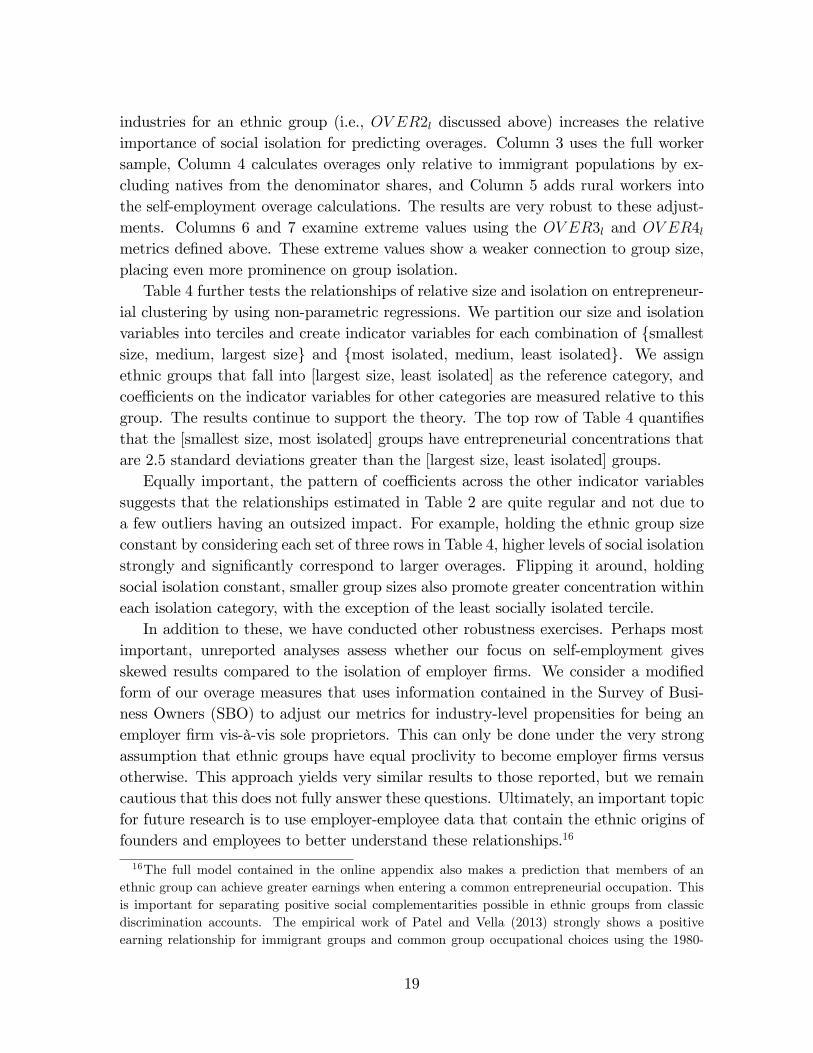
industries for an ethnic group (i.e., OV ER2l discussed above) increases the relativeimportance of social isolation for predicting overages. Column 3 uses the full workersample, Column 4 calculates overages only relative to immigrant populations by ex-cluding natives from the denominator shares, and Column 5 adds rural workers intothe self-employment overage calculations. The results are very robust to these adjust-ments. Columns 6 and 7 examine extreme values using the OV ER3l and OV ER4lmetrics defined above. These extreme values show a weaker connection to group size,placing even more prominence on group isolation.Table 4 further tests the relationships of relative size and isolation on entrepreneur-

ial clustering by using non-parametric regressions. We partition our size and isolationvariables into terciles and create indicator variables for each combination of {smallestsize, medium, largest size} and {most isolated, medium, least isolated}. We assignethnic groups that fall into [largest size, least isolated] as the reference category, andcoeffi cients on the indicator variables for other categories are measured relative to thisgroup. The results continue to support the theory. The top row of Table 4 quantifiesthat the [smallest size, most isolated] groups have entrepreneurial concentrations thatare 2.5 standard deviations greater than the [largest size, least isolated] groups.Equally important, the pattern of coeffi cients across the other indicator variables

suggests that the relationships estimated in Table 2 are quite regular and not due toa few outliers having an outsized impact. For example, holding the ethnic group sizeconstant by considering each set of three rows in Table 4, higher levels of social isolationstrongly and significantly correspond to larger overages. Flipping it around, holdingsocial isolation constant, smaller group sizes also promote greater concentration withineach isolation category, with the exception of the least socially isolated tercile.In addition to these, we have conducted other robustness exercises. Perhaps most

important, unreported analyses assess whether our focus on self-employment givesskewed results compared to the isolation of employer firms. We consider a modifiedform of our overage measures that uses information contained in the Survey of Busi-ness Owners (SBO) to adjust our metrics for industry-level propensities for being anemployer firm vis-à-vis sole proprietors. This can only be done under the very strongassumption that ethnic groups have equal proclivity to become employer firms versusotherwise. This approach yields very similar results to those reported, but we remaincautious that this does not fully answer these questions. Ultimately, an important topicfor future research is to use employer-employee data that contain the ethnic origins offounders and employees to better understand these relationships.16

16The full model contained in the online appendix also makes a prediction that members of anethnic group can achieve greater earnings when entering a common entrepreneurial occupation. Thisis important for separating positive social complementarities possible in ethnic groups from classicdiscrimination accounts. The empirical work of Patel and Vella (2013) strongly shows a positiveearning relationship for immigrant groups and common group occupational choices using the 1980-

19

3.5 IV Empirical Tests: 1980 Values

We next consider IV specifications to test against reverse causality concerns (e.g., thatisolated business ownerships lead to greater social isolation or lower group sizes). Weuse two sets of instruments. The first set of instruments builds upon an idea developedin our model, that initial conditions can have lasting and persistent impacts, whichis also shown quite strongly in this context by the empirical work of Patel and Vella(2013). We thus use the lagged 1980 values of ethnic group size and in-marriage ratesin the United States to instrument for 2000 levels. The distinct advantage of theseinstruments is that they can be calculated from the 1980 Census of Populations in amanner very comparable to our endogenous regressors. Despite this comparable datastructure and collection procedure, the ethnic divisions in 1980 are less detailed thanin 2000 and thus, in some cases, the same 1980 value must be applied to several 2000ethnic groups. We thus cluster standard errors around the 43 groups present in the 1980data, with other aspects of the IV estimations being the same as OLS specifications.The first-stage results with this instrument set are quite strong. The first two

columns of Table 5 show that these instruments have very strong individual predictivepower and a combined joint F-statistic of 24.17 The exclusion restriction requires thatthe 1980 group sizes and in-marriage levels only impact 2000 entrepreneurship to theextent that they shape current group size and social isolation, which seems reasonable.One possible counter to this, on the other hand, is that some of the 1980 respondentsare still employed in 2000, and this may carry with it persistence that violates theexclusion restriction.The second-stage results in Column 3 are quite similar to the OLS findings. The

IV specifications suggest that a one standard-deviation decrease in ethnic group sizeincreases overage by 0.76 standard deviations. A one standard-deviation increase inisolation leads to a 0.52 standard-deviation increase in entrepreneurial concentration.These results are well-measured and economically important. The size coeffi cient growsmodestly from its OLS baseline, while the in-marriage rate coeffi cient declines slightly.The results are precisely enough estimated that we can reject at a 5% level the null hy-pothesis in Wu-Hausman tests that the instrumented regressors are exogenous. TheseIV results strengthen the predictions of our theory that smaller, more isolated groupsare more conducive to entrepreneurial clustering.

2000 Census of Populations data, and Table A2 in the online appendix provides complementaryevidence using our data. Related work also includes Chiswick (1978), Borjas (1987), Simon andWarner (1992), Rauch (2001), Mandorff (2007), Bayer et al. (2008), and Beaman (2012).17The F-statistic comes from the Kleibergen-Paap Wald rank F-statistic used when standard errors

are clustered or robust and is based off the Cragg-Donald F-test for weak instrumentation.

20

3.6 IV Empirical Tests: Gravity Model and UK Values

Our second IV approach uses as instruments the predicted ethnic group size from agravity model and in-marriage rates from the United Kingdom in 1991. This is aneven stronger test of the model, with advantages and liabilities compared to our 1980instruments. First, to instrument for ethnic group size, we use a gravity model toquantify predicted ethnic size based upon worldwide migration rates to the UnitedStates. The original application of gravity models was to trade flows, where studiesshowed that countries closer to each other and with larger size tended to show greatertrade flows, similar to the forces of planetary pull. This concept has also been appliedto the migration literature, and we similarly model

SIZEl = α + β1DISTl + β2POPl + εl, (8)

where DISTl is the log distance to the United States from the origin country and POPlis the log population of the origin country. For this purpose, we estimate log ethnicgroup size in the United States as the dependent variable (without a negative valuebeing taken as in earlier estimations). Unsurprisingly, lower distance (β1 = −1.56(s.e.=0.22)) and greater population (β2 = 0.38 (s.e.=0.06)) are strong predictors ofethnic group size in the United States. We take the predicted values from this regressionfor each ethnic group as our first instrument.For our second instrument of in-marriage rates in the United States, we calculate

the in-marriage rates in the 1991 UK Census of Populations. This approach is attrac-tive as the social isolation evident in the United Kingdom a decade before our study isonly likely to be predictive of US self-employment rates to the extent that the Britishisolation captures a persistent trait of the ethnic group. The limitation of this instru-ment is that we are only able to calculate this for 24 broader ethnic sets than our baseobservations. We map our observations to these groups and cluster the standard errorsat the UK group level.Columns 4-5 of Table 5 again report the first-stage relationships. The instruments

remain individually predictive of their corresponding endogenous regressor, and theyhave a joint F-statistic of 35.5. Similar to the 1980 US instruments, the minimum2SLS relative bias that can be specified is less than 10%. This implies that we canspecify a very small bias and still reject the null hypothesis that the instruments areweak. The bias level is determined by the minimum eigenvalue statistic and Stock andYogo’s (2005) 2SLS size of the nominal 5% Wald test.The second-stage results are again comparable to our core OLS findings. The size

results are a bit lower than OLS, while the social isolation effects are even strongerthan OLS, with elasticities of around 0.67. We now fail to reject at a 5% level that theinstrumented regressors are exogenous, but we do reject it a 10% level.Table 6 shows a set of robustness checks with the two IV approaches. The results

21

are quite similar with the simple adjustments of excluding sample weights, droppingwinsorization, or using bootstrapped standard errors. We drop the robustness checksof median regressions and continent fixed effects, with the latter being due to our directuse of distance for predicted ethnic group size.The results with simulated overage controls are more interesting and deserve greater

comment. It becomes harder in the presence of the simulated overage controls for us toestablish a high-quality first stage for the size variable. This is workable enough in thecase of the 1980 size instrument, but it is not feasible for the predicted size relationshipin the gravity model. Intuitively, both the instrument and predicted overage are beingbuilt upon the same data, making it hard to separate them.Accordingly, in Columns 5 and 6, we start by just instrumenting for the isolation

metric, entering size and the predicted overage as control variables. These results arequite strong and comparable to the base IV. In Columns 7 and 8, we conduct thedouble IV for the 1980 instruments, which maintain a first-stage relationship, and findqualitatively similar results.Table 7 shows comparable patterns with the alternative metric designs. The results

for social isolation are robust in all specifications. Those for size are mostly robust, witha few exceptions in Panel B with the predicted size instruments. Table 8 also shows verysimilar results to those reported above when expanding the gravity equation to have asquared distance term or an indicator for Canada and Mexico as bordering countriesor when using underlying components of the gravity equation as direct instruments.In summary, and looking across the OLS and IV variants, the model developed in

this paper finds consistent support. The strongest findings are those for social isolation,which is a very strong predictor of entrepreneurial concentration. The weight of theevidence also supports that smaller group sizes promote entrepreneurial concentration.

4 Conclusions

By distinguishing between market interactions and social interactions, we have devel-oped a theory where social relationships reduce the cost of acquiring sector-specificskills for entrepreneurship. As a result, occupational choice reinforces initial group dif-ferences, and different ethnic groups cluster in different industries. The scale economiesgenerated by social relationships imply that social interactions, as opposed to marketinteractions, can result in favorable economic outcomes and self-employment conditionsfor minority groups. This is true when interactions are random or endogenous, witha key condition being that social relationships must not be close substitutes for oneanother for the broadest predictions to hold. A natural extension is to apply thesetheoretical concepts to the intergenerational transmission of skills and to follow occu-pational structure and entrepreneurial persistence across generations. This interaction

22

mechanism can also be applied to the study of the transmission of other types of skillsbeyond entrepreneurship.Taken as a whole, the Census data are consistent with social complementarities

in skill acquisition operating as a stratifying force, contributing to the persistence ofdifferences in occupational structure, entrepreneurship, and group inequality. Censusdata on occupational choice show that ethnic clustering is an important aspect of en-trepreneurial activity. Mean earnings and entrepreneurship are positively related atthe group level when controlling for other factors. Using intermarriage data in theCensus as a proxy for social interactions, we find that entrepreneurial groups social-ize mostly within their own group, and that stratification appears to increase within-marriage. These results are also consistent with the economic success and social iso-lation of specialized minority groups throughout history. We hope that the predictionsof this theory for ethnic entrepreneurship can be evaluated in settings outside of theUnited States given its general nature (Fairlie et al., 2010). Further connecting this toethnic enclaves and employer-employee data will also be powerful.

23

References

[1] Agrawal, Ajay, Devesh Kapur, and John McHale. 2008. How do spatial and socialproximity influence knowledge flows? Evidence from patent data. Journal ofUrban Economics 64: 258-269.

[2] Aldrich, Howard and Roger Waldinger. 1990. Ethnicity and entrepreneurship. An-nual Review of Sociology 16: 111-135.

[3] Andersson, Fredrik, Monica Garcia-Perez, John Haltiwanger, Kristin McCue, andSeth Sanders. 2009. Workplace concentration of immigrants. Working Paper.

[4] Andersson, Fredrik, Simon Burgess, and Julia Lane. 2012. Do as the neighbors do:The impact of social networks on immigrant employment. Working Paper.

[5] Åslund, Olof, Lena Hensvik, and Oskar Skans. 2012. Seeking similarity: Howimmigrants and natives manage in the labor market. Working Paper.

[6] Åstebro, Thomas, Holger Herz, Ramana Nanda, and Roberto Weber. 2014. Seek-ing the roots of Entrepreneurship: Insights from behavioral economics. Journalof Economic Perspectives 28: 49-70.

[7] Bayer, Patrick, Stephen Ross, and Giorgio Topa. 2008. Place of work and placeof residence: Informal hiring networks and labor market outcomes. Journal ofPolitical Economy 116: 1150-1180.

[8] Beaman, Lori. 2012. Social networks and the dynamics of labor market outcomes:Evidence from refugees resettled in the US. Review of Economic Studies 79:128-161.

[9] Becker, Gary. 1957. The Economics of Discrimination. Chicago: University ofChicago Press.

[10] Becker, Gary. 1973. A Theory of marriage: Part I. Journal of Political Economy81: 813-846.

[11] Bertrand, Marianne, Erzo Luttmer, and Sendhil Mullainathan. 2000. Networkeffects and welfare cultures. Quarterly Journal of Economics 115: 1019-1055.

[12] Bisin, Alberto and Thierry Verdier. 2000. Beyond the melting pot: Cultural trans-mission, marriage, and the evolution of ethnic and religious traits. QuarterlyJournal of Economics 115: 955-988.

[13] Bisin, Alberto, Giorgio Topa, and Thierry Verdier. 2004. Religious intermarriageand socialization in the United States. Journal of Political Economy 112: 615-664.

[14] Blalock, Hubert. 1967. Toward a Theory of Minority Group Relations. New York:John Wiley.

24

[15] Bonacich, Edna. 1973. A theory of middleman minorities. American SociologicalReview 38: 583-594.

[16] Borjas, George. 1987. Self-selection and the earnings of immigrants. AmericanEconomic Review 80: 531-553.

[17] Borjas, George. 1992. Ethnic capital and intergenerational mobility. QuarterlyJournal of Economics 107: 123-150.

[18] Borjas, George. 1995. Ethnicity, neighborhoods and human capital externalities.American Economic Review 85: 365-390.

[19] Botticini, Marestella and Zvi Eckstein. 2005. Jewish occupational selection: Edu-cation, restrictions, or minorities? Journal of Economic History 65: 922-948.

[20] Calvo-Armengol, Antoni and Matthew Jackson. 2004. The effects of social net-works on employment and inequality. American Economic Review 94: 426-454.

[21] Chiswick, Barry. 1978. The effect of Americanization on the earnings of foreign-born men. Journal of Political Economy 86: 897-921.

[22] Chung, Wilbur and Arturs Kalnins. 2006. Social capital, geography, and the sur-vival: Gujarati immigrant entrepreneurs in the U.S. lodging industry.Manage-ment Science 52(2): 233-247.

[23] Cohen, Robin. 1997. Global Diasporas: An Introduction. London: University Col-lege London Press.

[24] Dunn, Thomas and Douglas Holtz-Eakin. 2000. Financial capital, human capital,and the transition to self-employment: Evidence from intergenerational links.Journal of Labor Economics 18: 282-305.

[25] Durlauf, Steven and Marcel Fafchamps. 2006. Social capital. In Handbook of Eco-nomic Growth, edited by Philippe Aghion and Steven Durlauf. Amsterdam:North Holland.

[26] Durlauf, Steven and Yannis Ioannides, 2010. Social interactions. Annual Reviewof Economics 2: 451-478.

[27] Faggio, Giulia, and Olmo Silva. 2014. Self-employment and entrepreneurship inurban and rural labour markets. Journal of Urban Economics 83(1): 67-85.

[28] Fairlie, Robert. 2008. Estimating the Contribution of Immigrant Business Own-ers to the U.S. Economy. Small Business Administration, Offi ce of AdvocacyReport.

[29] Fairlie, Robert, Harry Krashinsky, and Julie Zissimopoulos. 2010. The interna-tional Asian business success story? A comparison of Chinese, Indian andother Asian businesses in the United States, Canada and United Kingdom.

25

In International Differences in Entrepreneurship, edited by Josh Lerner andAntoinette Schoar. Chicago: University of Chicago Press.

[30] Fairlie, Robert and Magnus Lofstrom. 2013. Immigration and entrepreneurship. InThe Handbook on the Economics of International Migration, edited by BarryChiswick and Paul Miller. Amsterdam: North-Holland Publishing.

[31] Fairlie, Robert and Alicia Robb. 2007. Families, human capital, and small business:Evidence from the Characteristics of Business Owners Survey. Industrial andLabor Relations Review 60: 225-245.

[32] Gil, Ricard and Wesley Hartmann. 2009. Airing your dirty laundry: Vertical in-tegration, reputational capital, and social networks. The Journal of Law, Eco-nomics, & Organization 27(2): 219-244.

[33] Glaeser, Edward, Bruce Sacerdote and José Scheinkman. 1996. Crime and socialinteractions. Quarterly Journal of Economics 111: 507-548.

[34] Glaeser, Edward and José Scheinkman. 2002. Non-market interaction. In Ad-vances in Economics and Econometrics: Theory and Applications, Eight WorldCongress, edited by Mathias Dewatripont, Lars Peter Hansen, and StephenTurnovsky. Cambridge, UK: Cambridge University Press.

[35] Granovetter, Mark. 1973. The strength of weak ties.American Journal of Sociology78: 1360-1380.

[36] Greif, Avner. 1993. Contract enforceability and economic institutions in earlytrade: The Maghribi traders coalition. American Economic Review 83: 525-548.

[37] Greif, Avner, Paul Milgrom, Barry and Weingast. 1994. Coordination, commit-ment and enforcement: The case of the merchant guild. Journal of PoliticalEconomy 102: 745-776.

[38] Hunt, Jennifer. (2011). Which immigrants are most innovative and entrepreneur-ial? Distinctions by entry visa. Journal of Labor Economics 29(3): 417-457.

[39] Jackson, C. Kirabo and Henry Schneider. 2011. Do social connections reduce moralhazard? Evidence from the New York City taxi industry. American EconomicJournal: Applied Economics 3(3): 244-267.

[40] Kennedy, Ruby. 1944. Single or triple melting-pot? Intermarriage trends in NewHaven, 1870-1940. The American Journal of Sociology 49: 331-339.

[41] Kerr, Sari Pekkala and William Kerr. 2015. Immigrant entrepreneurship. WorkingPaper, NBER Cambridge, MA.

26

[42] Kerr, Sari Pekkala, William Kerr, and William Lincoln. 2015. Skilled immigrationand the employment structures of U.S. firms. Journal of Labor Economics33(S1): S147-S186.

[43] Kerr, William. 2013. U.S. high-skilled immigration, innovation, and entrepreneur-ship: Empirical approaches and evidence. Working Paper no. 19377, NBER,Cambridge, MA.

[44] Kihlstrom, R., and Jean-Jacques Laffont. 1979. A general equilibrium entrepre-neurial theory of firm formation based on risk aversion. Journal of PoliticalEconomy 87: 719-748.

[45] Kirzner, Israel. 1972. Competition and Entrepreneurship. Chicago: University ofChicago Press.

[46] Kirzner, Israel. 1979. Perception, Opportunity and Profit; Studies in the Theoryof Entrepreneurship. Chicago: University of Chicago Press.

[47] Knight, Frank. 1921. Risk, Uncertainty, and Profit. Boston: Houghton Miffl in.

[48] Kuznets, Simon. 1960. Economic structure and life of the Jews. In The MinorityMembers: History, Culture, and Religion, edited by Louis Finkelstein. Philadel-phia, PA: Jewish Publication Society of America.

[49] Landa, Janet. 1981. A theory of the ethnically homogeneous middleman group: Aninstitutional alternative to contract law. Journal of Legal Studies 10: 349-362.

[50] Lazear, Edward. 1999. Culture and language. Journal of Political Economy 107:95-126.

[51] Lazear, Edward. 2005. Entrepreneurship. Journal of Labor Economics 23: 649-680.

[52] Light, Ivan. 1977. The ethnic vice industry, 1880-1944. American Sociological Re-view 42: 464-479.

[53] Lucas, Robert. 1978. On the size distribution of business firms. Bell Journal ofEconomics 9: 508-523.

[54] Mandorff, Martin. 2007. Social networks, ethnicity, and occupation. University ofChicago Ph.D. Dissertation.

[55] Manski, Charles. 1993. Identification of endogenous social effects: The reflectionproblem. Review of Economic Studies 60: 531-542.

[56] Melton, Gordon, ed. 1999. Encyclopedia of American Religions. 6th ed. Detroit:Gale Research.

[57] Milgrom, Paul, Douglass North, and BarryWeingast. 1990. The role of institutionsin the revival of trade: The medieval law merchant, private judges, and theChampagne fairs. Economics and Politics 1: 1-23.

27

[58] Montgomery, James. 1991. Social networks and labor-market outcomes: Towardan economic analysis. American Economic Review 81: 1408-1418.

[59] Morris, Stephen. 1956. Indians in East Africa: A study in a plural society. TheBritish Journal of Sociology 7: 194-211.

[60] Patel, Krishna and Francis Vella. 2013. Immigrant networks and their implicationsfor occupational choice and wages. Review of Economics and Statistics 95(4):1249-1277.

[61] Rauch, James. 2001. Business and social networks in international trade. Journalof Economic Literature 39: 1177-1203.

[62] Schumpeter, Joseph. 1942. Capitalism, Socialism, and Democracy. New York:Harper Brothers.

[63] Schumpeter, Joseph. 1988. Essays in Entrepreneurs, Innovations, Business Cy-cles, and the Evolution of Capitalism, edited by R. Clemence. Piscataway, NJ:Transaction Publishers.

[64] Simon, Curtis, and John Warner. 1992. Matchmaker, matchmaker: The effect ofold boy networks on job match quality, earnings and tenure. Journal of LaborEconomics 10(3): 306-330.

[65] Sowell, Thomas. 1981. Ethnic America. New York: Basic Books.

[66] Sowell, Thomas. 1996. Migrations and Cultures: A World View. New York: BasicBooks.

[67] Thernstrom, Stephan, ed. 1980.Harvard Encyclopedia of American Ethnic Groups.Cambridge, MA: Harvard University Press.

[68] Winder, R. Bayly. 1962. The Lebanese in West Africa. Comparative Studies inSociety and History 4: 296-333.

28

V(1,0)

V(0,1)

v

Q1

Q0

V(1,0)

V(0,1)

v

Q1

Q0

Figure 1: Production possibilities with specialized occupational distributions. The ray v is the preference parameter over goods in the Leontief utility function. Along the curve with the kink V(1,0), all entrepreneurs belong to group A (below the kink) or all members of group A are entrepreneurs (above). Similarly, along the curve with the kink V(0,1), all entrepreneurs belong to group B (below) or all members of group B are entrepreneurs (above).

V(1,0) v* V(0,1) v

X

1

0

XB

XA

V(1,0) v* V(0,1) v

X

1

0

XB

XA

Figure 2. The efficient occupational distribution for different values of v. The minority group A specializes as entrepreneurs so long as the entrepreneurial sector is small enough.

Ethnic group, designated by

country of origin or sub-groups available

in IPUMS

Weighted average

overage ratio over all

industries

Weighted average overage ratio for three

largest self-employment

industries for ethnicitySelf-employment industry with max

overage ratio

Total employment

in sample

Share of employment classified as

self-employed

In-marriage rate

Yemen 50.0 64.2 Grocery stores 2,322 26% 86%Eritrea 35.4 45.5 Taxicab service 3,338 17% 100%Gujarati 32.8 59.4 Hotels and motels 26,373 25% 93%Ethiopia 27.2 43.9 Taxicab service 8,760 14% 64%Bangladesh 20.5 27.6 Taxicab service 11,770 16% 86%Chaldean 16.1 35.0 Grocery stores 5,429 33% 88%Haiti 16.1 29.8 Taxicab service 58,971 8% 75%Ghana 15.9 20.6 Taxicab service 10,975 11% 68%Afghanistan 15.3 20.9 Taxicab service 6,432 24% 76%Nigeria 13.6 29.5 Taxicab service 27,232 18% 64%Tonga 12.0 14.5 Landscape and horticultural services 2,685 27% 77%Morocco 11.3 11.2 Construction 5,346 23% 32%Punjabi 10.5 21.8 Gasoline service stations 16,453 27% 96%Jordan 10.0 17.6 Grocery stores 7,674 35% 68%Laos 9.9 3.6 Agricultural production, crops 19,635 9% 77%Pakistan 9.9 18.5 Taxicab service 35,722 22% 83%Dominican Republic 8.7 16.6 Taxicab service 70,576 13% 62%Cambodia 8.5 7.8 Eating and drinking places 16,245 15% 82%Iraq 8.5 3.4 Offices and clinics of physicians 4,598 32% 60%Turkey 8.1 3.4 Eating and drinking places 10,438 27% 60%Korea 8.0 15.0 Laundry, cleaning, and garment services 91,928 45% 70%Australia 7.9 2.1 Construction 4,910 23% 32%Hungary 7.6 3.1 Construction 6,697 26% 32%Syria 7.5 11.0 Offices and clinics of physicians 7,623 41% 57%Sri Lanka (Ceylon) 7.3 9.1 Offices and clinics of physicians 4,010 26% 50%

Table 1a: Ethnic groups displaying the greatest self-employment industrial concentration

Notes: Descriptive statistics from 2000 Census IPUMS. Sample includes males immigrating after 1968 (effective date of the Immigration Reform Act of 1965), aged 30-65 in 2000, and living in the United States for at least 10 years. Sample excludes workers whose self-employment status is unknown or not applicable, industries without self-employment, and workers living outside of metropolitan areas. The overage ratios and industry titles are specific to self-employment and weight industries by the number of self-employed workers for the ethnic group. Two small groups that are partially composed of residual individuals are not listed in this table but have overage values in this range (Indochina, ns 9.4; Africa, ns/nec 8.2). The employment column displays the total workforce size included in the sample for each ethnic group.

Ethnic groupIndustry of max overage for self-

employed sample IndexIndustry

sizeIndustry of max overage for total

worker sampleIndustry

size Industry of max total employmentIndustry

size

Gujarati Hotels and motels 108.1 31 Liquor stores 146 Hotels and motels 31Yemen Grocery stores 75.0 13 Grocery stores 13 Grocery stores 13Eritrea Taxicab service 61.0 77 Taxicab service 77 Taxicab service 77Ethiopia Taxicab service 52.6 77 Taxicab service 77 Taxicab service 77Bangladesh Taxicab service 47.1 77 Taxicab service 77 Eating and drinking places 4Haiti Taxicab service 42.3 77 Taxicab service 77 Construction 1Nigeria Taxicab service 38.1 77 Taxicab service 77 Hospitals 5Ghana Taxicab service 35.3 77 Taxicab service 77 Hospitals 5Punjabi Gasoline service stations 34.6 88 Taxicab service 77 Taxicab service 77Korea Laundry, cleaning, etc. services 33.5 94 Shoe repair shops 200 Laundry, cleaning, etc. services 94Afghanistan Taxicab service 32.5 77 Taxicab service 77 Eating and drinking places 4Jordan Grocery stores 28.1 13 Taxicab service 77 Grocery stores 13Dom. Republic Taxicab service 27.2 77 Taxicab service 77 Construction 1Armenian Jewelry stores 25.7 138 Jewelry stores 138 Construction 1Pakistan Taxicab service 25.6 77 Taxicab service 77 Taxicab service 77Lebanon Gasoline service stations 23.5 88 Gasoline service stations 88 Eating and drinking places 4Chaldean Grocery stores 20.6 13 Liquor stores 146 Grocery stores 13Tonga Landscape/horticultural services 18.2 25 Landscape/horticultural services 25 Construction 1India Hotels and motels 17.8 31 Offices and clinics of physicians 36 Computer and data processing 8Portugal Fishing, hunting, and trapping 16.5 170 Dyeing and finishing textiles 176 Construction 1Ecuador Taxicab service 15.6 77 Apparel and accessories 106 Construction 1Iran Apparel, fabrics, and notions 14.3 144 Apparel, fabrics, and notions 144 Eating and drinking places 4Vietnam Fishing, hunting, and trapping 13.4 170 Fishing, hunting, and trapping 170 Electrical machinery/equipment 14USSR/Russia Taxicab service 13.2 77 Taxicab service 77 Construction 1Ukraine Taxicab service 13.2 77 Taxicab service 77 Construction 1

Notes: See Table 1a. Table is ordered by the 25 largest self-employment overage ratios at the industry level for ethnic groups. The industry size variable ranks industries from largest (1) to smallest (200). The table also displays for each ethnic group the industry of maximum overage when considering all employed workers and the industry where the greatest number of workers are employed.

Table 1b: Maximum overage clusters and industry employment ranks by ethnic group

Baseline estimation

Without sample weights

Without winsorization

Including fixed effects

for origin continent

Using median

regression format

Using bootstrapped

standard errors

Including simulated overage control1

Including simulated overage control2

(1) (2) (3) (4) (5) (6) (7) (8)

Inverse of log ethnic group size 0.634 0.630 0.629 0.552 0.586 0.630 0.509 0.524(small groups have larger values) (0.069) (0.067) (0.062) (0.070) (0.092) (0.070) (0.188) (0.182)

Log isolation of ethnic group 0.519 0.521 0.511 0.485 0.529 0.521 0.550 0.538(0.067) (0.065) (0.066) (0.091) (0.091) (0.070) (0.070) (0.067)

Log predicted overage1 0.155(0.195)

Log predicted overage2 0.123(0.186)

R-Squared value 0.612 0.626 0.629 0.650 0.428 0.626 0.577 0.612

Table 2: OLS estimations for log weighted average overage ratio for ethnic groups

Notes: Estimations describe the OLS relationship between industry concentration for ethnic entrepreneurship and ethnic group size and in-marriage isolation. The outcome variable is the log weighted average overage ratio across industries for each ethnic group, where the weights are levels of self employment in each industry per group. Variables are winsorized at their 10%/90% levels and transformed to have unit standard deviation for interpretation. Regressions are weighted by log ethnic group employee counts in MSAs, include 77 observations, and report robust standard errors. Columns 2-6 provide robustness checks on the baseline specification. Regressions in Columns 5 and 6 are unweighted and should be referenced against Column 2. Column 5 reports pseudo R-squared values. Columns 7 and 8 include control variables for predicted overage ratios based upon 1000 Monte Carlo simulations. In these simulations, pools of similarly sized ethnic groups to our true sample are formed and randomly assigned industry and entrepreneurship status according to national propensities. From these random assignments, we calculate 1000 overage metrics for each ethnic group that exactly mirror our primary data construction. The average of these simulations is entered as a control variable. In the first version included in Column 7, self-employment status and industry status are separately randomized, such that we overall predict roughly the same self-employment rate in each industry. In the second version included in Column 8, self-employment status and industry are jointly drawn such that we overall replicate observed self-employment levels across industries.

Baseline estimation

Using three largest

industries for ethnic group

Using total worker sample

Excluding natives from denominator

sharesIncluding

rural workers

(1) (2) (3) (4) (5) (6) (7)

Inverse of log ethnic group size 0.634 0.375 0.595 0.398 0.602 0.130 0.068(small groups have larger values) (0.069) (0.080) (0.073) (0.080) (0.072) (0.076) (0.076)

Log isolation of ethnic group 0.519 0.640 0.514 0.578 0.529 0.722 0.706(0.067) (0.072) (0.066) (0.083) (0.068) (0.070) (0.075)

R-Squared value 0.61 0.51 0.525 0.470 0.585 0.533 0.508

Notes: See Table 2. Regressions in Columns 2-5 provide robustness checks on the core metric. Column 2 restricts the overage measure to just the three largest self-employment industries for an ethnic group, Column 3 considers the metric that uses all employed workers for the ethnic group, Column 4 compares industry-level overages only to rates of other immigrant groups, and Column 5 includes rural workers in the sample. Columns 6-7 consider extreme values among industries by ethnic group. These latter overages are done without reference to industry importance in terms of ethnic group self-employment, but they do require at least ten observations exist for an ethnic group - industry cluster to be included.

Table 3: OLS estimations with alternative metric designs

Log weighted average overage across all industriesLog average

of three largest overage

ratios for ethnic group

Log largest overage ratio

for ethnic group

Log weighted average overage across all

industries

Log weighted average overage across three

largest industries

Log average of three largest overage ratios for

ethnic groupLog largest overage ratio

for ethnic group

(1) (2) (2) (3)

(0,1) Indicator: ethnic size in smallest third x 2.472 2.276 1.826 1.572(0,1) Indicator: ethnic isolation in highest third (0.188) (0.168) (0.155) (0.180)

(0,1) Indicator: ethnic size in smallest third x 1.514 0.753 0.416 0.375(0,1) Indicator: ethnic isolation in middle third (0.271) (0.380) (0.368) (0.362)

(0,1) Indicator: ethnic size in smallest third x 1.048 0.280 -0.654 -1.002(0,1) Indicator: ethnic isolation in lowest third (0.280) (0.273) (0.243) (0.251)

(0,1) Indicator: ethnic size in middle third x 1.581 1.211 1.127 1.044(0,1) Indicator: ethnic isolation in highest third (0.322) (0.374) (0.253) (0.260)

(0,1) Indicator: ethnic size in middle third x 0.908 0.573 0.351 0.338(0,1) Indicator: ethnic isolation in middle third (0.313) (0.314) (0.345) (0.362)

(0,1) Indicator: ethnic size in middle third x 0.428 -0.038 -0.443 -0.542(0,1) Indicator: ethnic isolation in lowest third (0.228) (0.220) (0.276) (0.306)

(0,1) Indicator: ethnic size in largest third x 0.802 0.944 0.927 0.767(0,1) Indicator: ethnic isolation in highest third (0.369) (0.361) (0.309) (0.300)

(0,1) Indicator: ethnic size in largest third x 0.126 0.279 0.329 0.294(0,1) Indicator: ethnic isolation in middle third (0.312) (0.334) (0.297) (0.299)

(0,1) Indicator: ethnic size in largest third x(0,1) Indicator: ethnic isolation in lowest third

R-Squared value 0.57 0.49 0.55 0.54

Table 4: OLS relationships with non-parametric forms

Notes: See Table 3. Effects are measured relative to largest and least isolated ethnic groups.

Excluded group

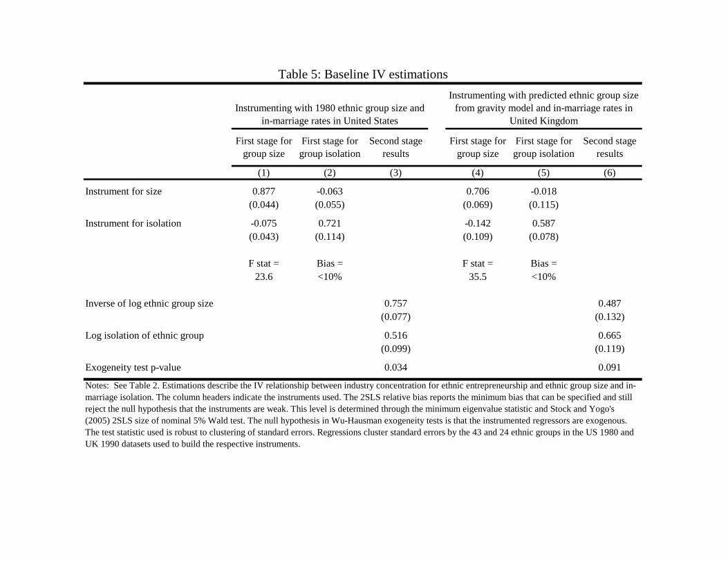
First stage for group size

First stage for group isolation

Second stage results

First stage for group size

First stage for group isolation

Second stage results

(1) (2) (3) (4) (5) (6)

Instrument for size 0.877 -0.063 0.706 -0.018(0.044) (0.055) (0.069) (0.115)

Instrument for isolation -0.075 0.721 -0.142 0.587(0.043) (0.114) (0.109) (0.078)

F stat = Bias = F stat = Bias =23.6 <10% 35.5 <10%

Inverse of log ethnic group size 0.757 0.487(0.077) (0.132)

Log isolation of ethnic group 0.516 0.665(0.099) (0.119)

Exogeneity test p-value 0.034 0.091

Table 5: Baseline IV estimations

Instrumenting with 1980 ethnic group size and in-marriage rates in United States

Instrumenting with predicted ethnic group size from gravity model and in-marriage rates in

United Kingdom

Notes: See Table 2. Estimations describe the IV relationship between industry concentration for ethnic entrepreneurship and ethnic group size and in-marriage isolation. The column headers indicate the instruments used. The 2SLS relative bias reports the minimum bias that can be specified and still reject the null hypothesis that the instruments are weak. This level is determined through the minimum eigenvalue statistic and Stock and Yogo's (2005) 2SLS size of nominal 5% Wald test. The null hypothesis in Wu-Hausman exogeneity tests is that the instrumented regressors are exogenous. The test statistic used is robust to clustering of standard errors. Regressions cluster standard errors by the 43 and 24 ethnic groups in the US 1980 and UK 1990 datasets used to build the respective instruments.

Baseline estimation

Without sample weights

Without winsorization

Using bootstrapped

standard errors

Including simulated overage control1

Including simulated overage control2

Including simulated overage control1

Including simulated overage control2

(1) (2) (3) (4) (5) (6) (7) (8)

Inverse of log ethnic group size 0.757 0.748 0.689 0.748 0.519 0.547 1.254 1.220(small groups have larger values) (0.077) (0.072) (0.084) (0.085) (0.232) (0.116) (0.355) (0.332)

Log isolation of ethnic group 0.516 0.526 0.554 0.526 0.539 0.516 0.465 0.468(0.099) (0.091) (0.145) (0.095) (0.122) (0.212) (0.133) (0.125)

F statistic 23.6 23.4 6.9 34.6 33.1 37.5 15.4 23.0Exogeneity test p-value 0.034 0.043 0.100 0.011 0.915 0.912 0.014 0.012

Inverse of log ethnic group size 0.487 0.476 0.506 0.476 0.315 0.334 Insufficient Insufficient(small groups have larger values) (0.132) (0.123) (0.091) (0.105) (0.185) (0.179) first stage first stage

Log isolation of ethnic group 0.665 0.639 0.464 0.639 0.772 0.751(0.119) (0.111) (0.089) (0.135) (0.089) (0.091)

F statistic 35.5 34.1 13.5 20.0 40.7 29.8Exogeneity test p-value 0.091 0.084 0.160 0.061 0.137 0.166

Table 6: Robustness checks on IV estimations for log weighted average overage ratio for ethnic groups

Notes: See Tables 2 and 5.

B. IV results using predicted group sizes and UK in-marriage rates

A. IV results using 1980 ethnic group size and in-marriage rates in United States

Double IVIsolation IV Only

Baseline estimation

Using three largest

industries for ethnic group

Using total worker sample

Excluding natives from denominator

sharesIncluding

rural workers

(1) (2) (3) (4) (5) (6) (7)

Inverse of log ethnic group size 0.757 0.531 0.636 0.491 0.730 0.272 0.193(small groups have larger values) (0.077) (0.110) (0.063) (0.135) (0.086) (0.126) (0.123)

Log isolation of ethnic group 0.516 0.696 0.469 0.771 0.532 0.759 0.720(0.099) (0.091) (0.104) (0.113) (0.097) (0.087) (0.107)

F statistic 23.6 23.6 54.4 23.6 23.6 23.6 23.6Exogeneity test p-value 0.034 0.019 0.403 0.081 0.040 0.042 0.078

Inverse of log ethnic group size 0.487 0.132 0.466 0.386 0.444 0.075 0.043(small groups have larger values) (0.132) (0.109) (0.120) (0.141) (0.132) (0.100) (0.090)

Log isolation of ethnic group 0.665 0.861 0.550 0.696 0.712 0.905 0.853(0.119) (0.125) (0.177) (0.130) (0.122) (0.104) (0.088)

F statistic 35.5 35.5 10.5 35.5 35.5 35.5 35.5Exogeneity test p-value 0.091 0.022 0.107 0.687 0.055 0.239 0.464

Notes: See Tables 3 and 5.

B. IV results using predicted group sizes and UK in-marriage rates

A. IV results using 1980 ethnic group size and in-marriage rates in United States

Table 7: IV estimations with alternative metric designs

Log weighted average overage across all industriesLog average

of three largest overage

ratios for ethnic group

Log largest overage ratio

for ethnic group

Baseline estimation

Including border in the gravity model

Including distance

squared in the gravity model

Using distance and population as instruments

Using distance, population, and

border as instruments

Using distance, population, and

distance squared as instruments

(1) (2) (3) (4) (5) (6)

Inverse of log ethnic group size 0.487 0.483 0.483 0.522 0.524 0.522(small groups have larger values) (0.132) (0.131) (0.130) (0.149) (0.148) (0.150)

Log isolation of ethnic group 0.665 0.665 0.665 0.680 0.624 0.673(0.119) (0.120) (0.120) (0.111) (0.084) (0.083)

F statistic 35.5 36.2 35.8 22.2 17.0 17.0Exogeneity test p-value 0.091 0.086 0.096 0.029 0.063 0.024Overidentification test p-value 0.174 0.283 0.394

Notes: See Tables 3 and 5.

Table 8: IV results with alternative gravity model designs for predicted size

Online Appendices

1 Theoretical Appendix

The theory in this paper consists of two fundamental building blocks. First, social in-teractions and production are complementary. Second, different social relationships arenot close substitutes for one another. The former is analyzed in the main text, and thisappendix begins with the omitted proofs and additional discussion. We then considerpricing equilibrium and social networks with endogenous matching. The numbering ofassumptions and propositions continues from the main text.

1.1 Proofs and Discussion of Baseline Model

1.1.1 Proofs of Propositions and Lemmas

Proposition 1 If v ≤ V (1, 0), all self-employed entrepreneurs in industry 1 belongto minority group A.

Proof: Take the distribution (XA, 0) where XA is such that v = V (XA, 0). This isfeasible since v ≤ V (1, 0). Assume by contradiction that it is not the uniquely effi cientdistribution. Then there exists an alternative distribution (X ′A, X

′B) with Q′1 ≥ Q1

and Q′0 ≥ Q0. Given Q′0 ≥ Q0 it follows that M ′ ≤ M , or equivalently, X ′ANA +

X ′BNB ≤ XANA, which implies X ′A ≤ XA and X ′B < XA, with X ′A < XA if X ′B = 0.Manipulating the expression for Q′1:

Q′1 = (M ′ −X ′BNB) θ (X ′A) +X ′BNBθ (X ′B) (1)

< (M −X ′BNB) θ (XA) +X ′BNBθ (XA) = Q1

This contradicts Q′1 ≥ Q1. �

Lemma If productivity is convex, both groups never work in both industries.

Proof: Assume by contradiction that an effi cient distribution (XA, XB) exists where0 < Xl < 1 for l = {A,B}. Consider a marginal change ε in the ethnic compositionof self-employed entrepreneurs in industry 1 while holding fixed the overall number ofsaid entrepreneurs M (and therefore also the outputs of both industries). Taking thederivative of Q1 with respect to ε, and evaluating it at ε = 0:

∂Q1∂ε

(XA +

ε

NA

, XB −ε

NB

)= θ (XA) +XAθ

′ (XA)− θ (XB)−XBθ′ (XB) (2)

1

Since (XA, XB) is effi cient, and since Xl is interior, this derivative has to be zero.1 Butwith convex productivity the derivative is zero only at XA = XB, which is the globalminimum. This contradicts effi ciency. �

Proposition 2 If productivity is convex, there is a cutoff value v∗ such that forv < v∗, the minority group specializes as self-employed entrepreneurs in industry 1,whereas for v > v∗, the majority specializes.

Proof: Direct from Proposition 1 and Lemma proofs with convexity. �

1.1.2 The Case of Non-Convex Productivity

To see that convexity is needed for the Lemma on ethnic homogeneity to hold, con-sider a non-convex production function where a threshold fraction must work as self-employed entrepreneurs in industry 1 for interaction to have value: θ > 0 if Xl ≥ b

and zero otherwise. This specification violates the assumption that productivity isstrictly increasing in the degree of specialization. Then, if the demand for industry 1output is so great that a single group cannot satisfy it entirely, v > V (0, 1), and ifin addition V (b, b) < v < V (b, 1), effi ciency requires that both ethnic groups work inboth industries, contradicting the Lemma.To see why, consider what would happen if one of the groups specialized completely.

In this case the non-specialized group’s degree of specialization would be positive butbelow b, causing the self-employed industry 1 entrepreneurs in that group to have zeroproductivity. If, however, the industrial distribution was unspecialized instead, withXA = XB, then self-employed industry 1 entrepreneurs in both groups would be asproductive as those in the most productive group were under the alternative. Clearlythis would be Pareto superior, contradicting the Lemma. This special case showshow the Lemma fails for non-convex productivity, and how in this case the qualitativefeatures of specialization will depend on specific functional form assumptions. Recallhowever that the results for both v ≤ V (1, 0) and v = V (0, 1) are more general andapply both for convex and non-convex productivity. This condition is less importantfor the remaining model discussion.

1.2 The Price Equilibrium

The model in the main text characterizes the effi cient outcome. The focus now turnsto the competitive outcome. An equilibrium analysis will yield two insights into how

1If the derivative is nonzero, then the output of industry 1 could increase while keeping the outputof industry 0 constant. By subsequently increasing the number of workers in industry 0 marginally, aPareto improvement is feasible, thus contradicting effi ciency.

2

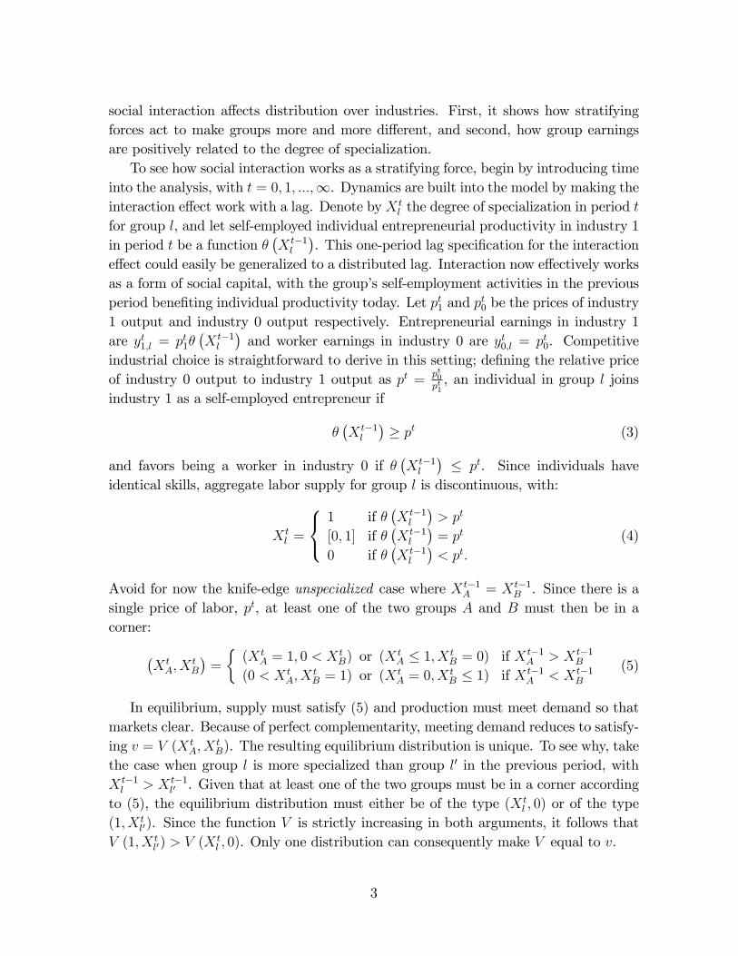
social interaction affects distribution over industries. First, it shows how stratifyingforces act to make groups more and more different, and second, how group earningsare positively related to the degree of specialization.To see how social interaction works as a stratifying force, begin by introducing time

into the analysis, with t = 0, 1, ...,∞. Dynamics are built into the model by making theinteraction effect work with a lag. Denote by X t

l the degree of specialization in period tfor group l, and let self-employed individual entrepreneurial productivity in industry 1in period t be a function θ

(X t−1l

). This one-period lag specification for the interaction

effect could easily be generalized to a distributed lag. Interaction now effectively worksas a form of social capital, with the group’s self-employment activities in the previousperiod benefiting individual productivity today. Let pt1 and p

t0 be the prices of industry

1 output and industry 0 output respectively. Entrepreneurial earnings in industry 1are yt1,l = pt1θ

(X t−1l

)and worker earnings in industry 0 are yt0,l = pt0. Competitive

industrial choice is straightforward to derive in this setting; defining the relative priceof industry 0 output to industry 1 output as pt =

pt0pt1, an individual in group l joins

industry 1 as a self-employed entrepreneur if

θ(X t−1l

)≥ pt (3)

and favors being a worker in industry 0 if θ(X t−1l

)≤ pt. Since individuals have

identical skills, aggregate labor supply for group l is discontinuous, with:

X tl =

1 if θ

(X t−1l

)> pt

[0, 1] if θ(X t−1l

)= pt

0 if θ(X t−1l

)< pt.

(4)

Avoid for now the knife-edge unspecialized case where X t−1A = X t−1

B . Since there is asingle price of labor, pt, at least one of the two groups A and B must then be in acorner:(

X tA, X

tB

)=

{(X t

A = 1, 0 < X tB) or (X t

A ≤ 1, X tB = 0) if X t−1

A > X t−1B

(0 < X tA, X

tB = 1) or (X t

A = 0, X tB ≤ 1) if X t−1

A < X t−1B

(5)

In equilibrium, supply must satisfy (5) and production must meet demand so thatmarkets clear. Because of perfect complementarity, meeting demand reduces to satisfy-ing v = V (X t

A, XtB). The resulting equilibrium distribution is unique. To see why, take

the case when group l is more specialized than group l′ in the previous period, withX t−1l > X t−1

l′ . Given that at least one of the two groups must be in a corner accordingto (5), the equilibrium distribution must either be of the type (X t

l , 0) or of the type(1, X t

l′). Since the function V is strictly increasing in both arguments, it follows thatV (1, X t

l′) > V (X tl , 0). Only one distribution can consequently make V equal to v.

3

The equilibrium distribution is therefore uniquely determined by the distributionin the previous period. Continuing to avoid the knife-edge unspecialized case, define afunction φ that maps every previous distribution into a new distribution:(

X tA, X

tB

)= φ

(X t−1A , X t−1

B

)(6)

Next, proceed to characterize stationary equilibrium distributions. Like other equilib-rium distributions, stationary distributions must satisfy (5) and must meet demand.Following the same argument as above, based on V being strictly increasing in botharguments, it follows that there is a stationary equilibrium where each of the twogroups specializes. Denote the stationary distribution as

(XAA , X

AB

)when the minority

specializes, and the stationary distribution as(XBA , X

BB

)when the majority specializes.

Finally, returning for a moment to the unspecialized knife-edge case where X t−1A =

X t−1B , this type of initial condition is of measure zero and therefore not elaborated

on. Note only that since V is strictly increasing in both arguments, there can only beone such stationary unspecialized equilibrium distribution. Denote that equilibriumdistribution as

(XUA , X

UB

). In the unspecialized case, although there is only one sta-

tionary equilibrium, the uniqueness of equilibria no longer applies. To summarize, thereare consequently three stationary equilibrium distributions: two specialized,

(XAA , X

AB

)and

(XBA , X

BB

), and one unspecialized,

(XUA , X

UB

). Figure A1 shows the two specialized

equilibria, as well as the knife-edge equilibrium, when v is less than V (1, 0).

1.2.1 Industrial Stratification

Our next analysis shows that the dynamic system in (6) converges to a stationaryspecialized equilibrium, so long as the interaction externality is not too strong. Thisanalysis only examines unspecialized initial conditions, which establishes convergenceon measure one. Consider what happens to the aggregate production of industry 1when one (infinitesimal) person in group l becomes a self-employed entrepreneur in thatindustry. First, aggregate production increases by an amount equal to the individualproductivity of that person, θ (Xl). In addition, all other self-employed entrepreneursin industry 1 from group l benefit from the interaction externality when socializing withthis new entrepreneur. Individual productivity therefore increases by 1

Nlθ′ (Xl) for all

XlNl self-employed industry 1 entrepreneurs in group l. Consequently, the internalizedeffect on aggregate production of one person joining the self-employed entrepreneurialsector of industry 1 is θ (Xl), and the external effect is Xlθ

′ (Xl). Assume that theexternal effect is smaller than the internal effect.2

Assumption 2 The internal effect dominates: θ′ (Xl)Xl < θ (Xl).

2We thank Rachel Soloveichik for this interpretation of Assumption 2.

4

This condition is satisfied if productivity is concave in Xl, but it also holds for someconvexity as long as θ (0) > 0. To see why the assumption is needed for the system tobe stable, consider the extreme case when group A has no mass at all, with NA = 0.Since the derivative of V with respect to X t

A is zero in this case, group A can be ignoredaltogether in the general equilibrium analysis. There is then a single stationary levelof specialization for group B; denote this value as X∗B.Consider a perturbation in period t so that the majority starts out with too many

entrepreneurs in industry 1, X tB > X∗B, shown in Figure A2. Such a deviation boosts

the interaction effect in period t + 1 relative to the stationary equilibrium, θ (X tB) >

θ (X∗B). With perfect complementarity, the outputs of both industry 0 and industry 1must therefore increase relative to their stationary equivalents. Increasing the outputof industry 0 requires an increase in the number of workers in that industry, andconsequently, a decrease in the number of self-employed entrepreneurs in industry 1 tobelow the stationary value X∗B. With fewer of these entrepreneurs in period t+ 1 thanthe stationary number, the tables turn in period t + 2, so that the interaction effectnow is reduced to below that in the stationary equilibrium. Reducing the productionof industry 0 and industry 1 in period t + 2 in response, the number of industry 0workers in period t + 2 has to decrease and the number of self-employed industry 1entrepreneurs has to increase relative to the stationary equilibrium. These reversalsrepeat every period in cobweb-style dynamics.3

The question of whether the system is stable reduces to whether the number ofself-employed entrepreneurs in industry 1 in period t + 2 is less than the number ofsuch entrepreneurs in period t, so that the degree of specialization in group B getscloser and closer to the stationary value X∗B over time. Using the derived directionof the change in industry 1 production, Qt+1

1 > Qt+21 , this latter inequality can be

equivalently expressed, after multiplying and dividing the left-hand side by X tB and

dividing both sides by X t+1B NB, as:

X tB

θ (X tB)

X tB

> X t+2B

θ(X t+1B

)X t+1B

(7)

Given that productivity is not too convex, as stipulated by Assumption 2, it followsthat θ(Xl)

Xlis strictly decreasing in Xl. Since X t

B > X t+1B , equation (7) then establishes

that X tB > X t+2

B . This proves convergence and the stability of group B’s degree ofspecialization around X∗B.Having established stability in the case of NA = 0, the same example also serves

to show how the stratifying force comes into play. Let group B be in its stable state,with X t

B = X∗B, and perturb the minority’s industry distribution so that XtA > X∗B.

3The flip-flopping character of the equilibrium distribution is a result of the one-period lag speci-fication for the interaction effect. The distribution would change more gradually with a more generalspecification allowing for distributed lags.

5

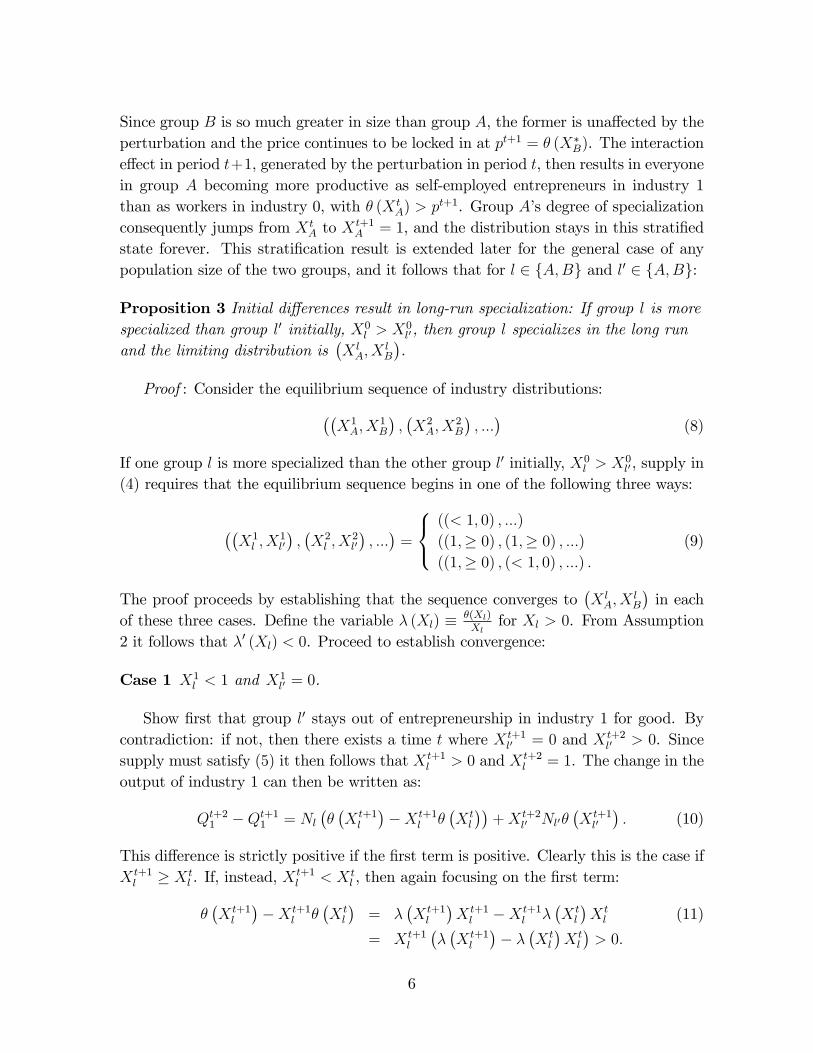
Since group B is so much greater in size than group A, the former is unaffected by theperturbation and the price continues to be locked in at pt+1 = θ (X∗B). The interactioneffect in period t+1, generated by the perturbation in period t, then results in everyonein group A becoming more productive as self-employed entrepreneurs in industry 1than as workers in industry 0, with θ (X t

A) > pt+1. Group A’s degree of specializationconsequently jumps from X t

A to Xt+1A = 1, and the distribution stays in this stratified

state forever. This stratification result is extended later for the general case of anypopulation size of the two groups, and it follows that for l ∈ {A,B} and l′ ∈ {A,B}:

Proposition 3 Initial differences result in long-run specialization: If group l is morespecialized than group l′ initially, X0

l > X0l′, then group l specializes in the long run

and the limiting distribution is(X lA, X

lB

).

Proof : Consider the equilibrium sequence of industry distributions:((X1A, X

1B

),(X2A, X

2B

), ...)

(8)

If one group l is more specialized than the other group l′ initially, X0l > X0

l′ , supply in(4) requires that the equilibrium sequence begins in one of the following three ways:

((X1l , X

1l′),(X2l , X

2l′), ...)

=

((< 1, 0) , ...)

((1,≥ 0) , (1,≥ 0) , ...)

((1,≥ 0) , (< 1, 0) , ...) .

(9)

The proof proceeds by establishing that the sequence converges to(X lA, X

lB

)in each

of these three cases. Define the variable λ (Xl) ≡ θ(Xl)Xl

for Xl > 0. From Assumption2 it follows that λ′ (Xl) < 0. Proceed to establish convergence:

Case 1 X1l < 1 and X1

l′ = 0.

Show first that group l′ stays out of entrepreneurship in industry 1 for good. Bycontradiction: if not, then there exists a time t where X t+1

l′ = 0 and X t+2l′ > 0. Since

supply must satisfy (5) it then follows that X t+1l > 0 and X t+2

l = 1. The change in theoutput of industry 1 can then be written as:

Qt+21 −Qt+1

1 = Nl

(θ(X t+1l

)−X t+1

l θ(X tl

))+X t+2

l′ Nl′θ(X t+1l′

). (10)

This difference is strictly positive if the first term is positive. Clearly this is the case ifX t+1l ≥ X t

l . If, instead, Xt+1l < X t

l , then again focusing on the first term:

θ(X t+1l

)−X t+1

l θ(X tl

)= λ

(X t+1l

)X t+1l −X t+1

l λ(X tl

)X tl (11)

= X t+1l

(λ(X t+1l

)− λ

(X tl

)X tl

)> 0.

6

This establishes thatQt+21 > Qt+1

1 . Since the output production of both industries mustmove in the same direction to clear the market, because of perfect complementarity, itfollows that the output of industry 0 also increases from t + 1 to t + 2. This in turnrequires that the number of workers in industry 0 increases, or equivalently, that thenumber of self-employed entrepreneurs in industry 1 decreases:

X t+2l Nl +X t+2

l′ Nl′ < X t+1l Nl +X t+1

l′ Nl′ . (12)

Since X t+2l = 1 and X t+1

l′ = 0, this inequality can be simplified as Nl + X t+2l′ Nl′ <

X t+1l Nl. This inequality is a contradiction and establishes that group l′ stays out

of self-employed entrepreneurship in industry 1 for good. The stationary equilibriummust consequently be of the form

(X ll , 0).

Assume first that X tl > X∗, in which case it is easy to show that Qt+1

1 > Ql1 > Qt+2

1

as well as X t+1l < X l

l < X t+2l . Since Qt+1

1 > Qt+21 it follows that:

X t+1l NAθ

(X tl

)> X t+2

l NAθ(X t+1l

)(13)

X t+1l λ

(X tl

)X tl > X t+2

l λ(X t+1l

)X t+1l

X tlλ(X tl

)> X t+2

l λ(X t+1l

).

The last line implies that X tl > X t+2

l . The exact same argument, but with reverseinequalities, can be made for X t

l < X ll . Therefore, having established that X t

l >

X t+2l > X l

l when Xtl > X l

l , and vice versa when Xtl < X l

l , it has been shown that Xtl

approaches the stationary equilibrium valueX ll over time. This establishes convergence

in Case 1.

Case 2 X1l = 1, X1

l′ ≥ 0, X2l = 1 and X2

l′ ≥ 0.

Show first that in this case, group l stays specialized for good. By contradiction:if not, then there exists a time t when X t

l = 1, X t+1l = 1 and X t+2

l < 1. Since supplymust satisfy (5), it follows that X t+2

l′ = 0. The change in the output of industry 1 canbe written as

Qt+21 −Qt+1

1 = Nl

(X t+2l θ (1)− θ (1)

)−X t+1

l′ Nl′θ(X tl

)< 0. (14)

Since the supply of output of both industries must move in the same direction to clearthe market, it follows that the output of industry 0 also decreases, which requires thatthe number of self-employed entrepreneurs in industry 1 increases:

X t+2l Nl +X t+2

l′ Nl′ > X t+1l Nl +X t+1

l′ Nl′ . (15)

Since X t+2l′ = 0 and X t+1

l = 1, this inequality can be rewritten as X t+2l Nl > Nl +

X t+1l′ Nl′ , which is a contradiction. This establishes that group l stays specialized in

7

industry 1 for good. The stationary equilibrium must consequently be of the form(1, X l

l′

). By the same argument as in Case 1, the sequence can be shown to approach

the stationary equilibrium value X ll′ over time, both if X

tl′ > X l

l′ and if Xtl′ < X l

l′ . Thisestablishes convergence in Case 2.

Case 3 X1l = 1 and X1

l′ ≥ 0 and X2l < 1 and X2

l′ = 0.

By the same argument in Case 1, it follows that group l′ stays out of entrepreneur-ship in industry 1 permanently. Repeating the arguments in Case 1, convergence canthen be established also in Case 3.

Consequently, in all three cases there is convergence. �This also implies that the stationary unspecialized equilibrium

(XUA , X

UB

)is un-

stable. If the minority group is slightly more specialized initially, then the economyconverges to minority specialization

(XAA , X

AB

), and if the opposite is true, then the

economy converges to majority specialization(XBA , X

BB

). Over time, social segregation

amplifies initial group differences.

1.2.2 Initial Conditions and Multiple Groups

Depending on the initial conditions, as is clear from Proposition 3, either of the twogroups A and B can specialize as self-employed entrepreneurs in industry 1. Socialinteraction amplifies initial differences, but it does not explain why they are thereto begin with. The difference in group size has some implications for what initialconditions to expect, however.Consider an economy with more than two groups. As before, the group with more

self-employed entrepreneurs in industry 1 initially will specialize in the long run. Ifthe initial industrial distribution is subject to randomness, one of the smaller groups islikely to be the most specialized initially. To see why, let the initial distribution be gen-erated by random draws, where each person becomes a self-employed entrepreneur inindustry 1 with probability ρ.4 This probability structure results in the same expectedinitial degree of specialization for all groups, but since the population size varies acrossgroups, the variance in the degree of specialization also varies. The smallest groupshave the largest variance, and therefore, the smallest groups are most likely to exhibitthe lowest and also the greatest initial degrees of specialization. Consequently, withthe smallest groups the most likely to specialize initially, as interaction amplifies initialdifferences over time, the smallest groups are also the most likely to specialize in thelong run.

4These draws can be partially correlated within groups with the assumption that the correlationis the same for every group.

8

1.2.3 Assimilation

Our model does not feature assimilation of immigrants and their offspring and thusyields permanent social and industrial segregation. In our framework, assimilationwould reduce the social isolation of an ethnic group (or some members of it) to themajority group. Our framework then predicts the industry choices of the assimilatedindividuals to look like those of the majority, especially if another ethnic group showsstrong social isolation.

1.2.4 Heterogeneity and Earnings

Social complementarities also have implications for earnings. To examine how inter-action effects would show up in earnings data, it is necessary to move away from theframework of identical skills. Returning to a static environment, endow each person iwith entrepreneurial skills relevant to self-employment in industry 1, s1 (i), and withanother set of skills necessary for industry 0, s0 (i). Self-employed entrepreneurial earn-ings in industry 1 are now a function of both interactions and skills. Denote the earningsof individual i in group l when she is a self- employed entrepreneur in industry 1 asy1 (Xl, i) = p1θ (Xl) s1 (i), and when she is a member of industry 0 as y0 (i) = p0s0 (i).Defining the ratios s ≡ s1

s0, p ≡ p0

p1, and q ≡ py1

y0, the earnings-maximizing industry

choice of individual i is to consider becoming a self-employed entrepreneur in industry1 if:

q (Xl, i) ≥ p (16)

and to consider working in industry 0 if q (Xl, i) ≤ p. Here the term q (Xl, i) =

θ (Xl) s (i) summarizes the individual’s comparative advantage in self-employed entre-preneurship in industry 1, at parity prices, as a function of social interaction and skills.When individuals have different skills, the character of the price equilibrium de-

pends crucially on the marginal self-employed entrepreneur and how her comparativeadvantage changes as more and more untalented people also become entrepreneurs inindustry 1. If the benefits of interaction are weak and the marginal entrepreneur “dete-riorates”as more intrinsically untalented people enter the industry, then the economyreduces to a standard Roy model, or sorting model, with a unique unspecialized equi-librium. Only if the interaction effect is strong enough to overcome skill heterogeneitycan interaction change the character of the equilibrium.Without loss of generality, order individuals from the greatest to the smallest com-

parative advantage in industry 1-style entrepreneurship, so that the skill ratio is de-creasing in i, s′ (i) ≤ 0. The marginal entrepreneur is then the individual indexed byi = Xl, and her comparative advantage is q (Xl, Xl). To prevent the economy fromreducing to a sorting model, assume that the interaction effect trumps heterogeneity:

Assumption 3 Interaction dominates at the margin: ddXl

q (Xl, Xl) > 0.

9

This assumption implies that the solid line in Figure A3 is upward sloping. Theequilibrium distribution (XA, XB) must be competitively supplied and enough outputmust be produced by both industries to meet demand. Using a similar line of reasoningas in the previous section, based on V being strictly increasing in both arguments, itfollows from Assumption 3 that there are three equilibria: one unstratified, denoted(XUA , X

UB

); one where the minority group A specializes, denoted

(XAA , X

AB

); and one

where the majority group B specializes, denoted(XBA , X

BB

).5

In the equilibrium where minority A specializes as self-employed entrepreneurs inindustry 1, the mean earnings of members of group A are higher than the mean earningsof members of group B, and vice versa in the equilibrium where group B specializes.To see why, let y = max (y0, y1) be actual individual earnings, and denote mean groupearnings as µ =

∫ 10ydi.

Proposition 4 Earnings covary with self-employed entrepreneurship in industry 1:µ (Xl) > µ (Xl′) if Xl > Xl′.

Proof: Since people sort into industries, mean earnings can be rewritten as

µ (Xl) =

∫ 1

0

y0 (i) di+

∫ Xl

0

(y1 (Xl, i)− y0 (i)) di (17)

Rearranging, the difference in mean earnings between the two groups is:

µ (Xl)− µ (Xl′) =

∫ Xl′

0

(y1 (Xl, i)− y1 (Xl′ , i)) di+

∫ Xl

Xl′

(y1 (Xl, i)− y0 (i)) di (18)

where both parts of the expression are positive. The first part is strictly positive due tothe interaction effect, ∂y1(Xl,i)

∂Xl> 0, and the second part is positive because of sorting,

y1 (Xl, i) ≥ y0 (i) for all i ≤ Xl. �This unequivocal effect on mean earnings at the group level does not carry through

to the industry level. Depending on the joint distribution of skills, mean earningsin either industry can increase or decrease as interaction increases self-employed en-trepreneurial productivity in industry 1 and shifts people of different ability betweenindustries. The effect of interaction on industry earnings is similar to the effect ofchanging skill prices, which cannot be signed for a general skill distribution (Heckmanand Honore, 1990).The difference in mean earnings, normalized in units of industry 0 output, is shown

in Figure A4 for the equilibrium with minority specialization. The exact derivationis included below. The relative price of industry 0 to industry 1 outputs is always

5Note that Assumptions 2 and 3, when combined, put both an upper and a lower bound on theinteraction effect: −d ln sdXl

< d ln θdXl

< 1Xl.

10

such that the marginal entrepreneur is indifferent between industries. Keeping trackof whether the marginal entrepreneur is in group A or in group B depending on theindustrial distribution, the equilibrium price can be expressed as:

p =

{q (Xl, Xl) if Xl > Xl′ and Xl′ = 0, or Xl < Xl′ and Xl > 0

q (Xl′ , Xl′) if Xl > Xl′ and Xl′ > 0, or Xl < Xl′ and Xl = 0(19)

When increasing the number of self-employed entrepreneurs in industry 1 in equilibriumwith minority specialization, the relative price of industry 0 output to industry 1 outputincreases continuously as the marginal entrepreneur in group A becomes more and moreproductive. This increase in price continues until all As are self-employed entrepreneursin industry 1. To expand industry 1’s self-employed entrepreneurial sector further fromthe point where everyone in group A are entrepreneurs, the price has to drop discretelyfrom p = q (1, 1) to q (0, 0), to lure the unproductive Bs into the sector as well. Theearnings differential between groups A and B moves accordingly, as shown in FigureA4, increasing continuously until all As are self-employed entrepreneurs in industry1, at which point earnings jump in response to the discontinuous drop in the relativeprice.Derivation of Earnings Differential in Figure A4: Mean earnings denominated in

terms of industry 0 outputs are:

µ (Xl)

p0=

∫ Xl

0

p−1θ (Xl) s1 (i) di+

∫ 1

Xl

s0 (i) di. (20)

Replace the relative price of industry 0 output to industry 1 output, p = p0p1, with the

comparative advantage of the marginal entrepreneur, q, since these two are equal inequilibrium. Denote the earnings differential as ∆ (Xl, Xl′) ≡ µ(Xl)−µ(Xl′ )

p0. It can be

expressed as:

∆ (Xl, Xl′) =

∫ Xl′

0

q−1 (θ (Xl)− θ (Xl′)) s1 (i) di+

∫ Xl

Xl′

[q−1θ (Xl) s1 (i)− s0 (i)

]di.

(21)For Xl < 1 and Xl′ = 0, where q = q (Xl, Xl), and q (Xl, Xl) = θ (Xl) s (Xl), differenti-ating with respect to Xl gives

∂∆ (Xl, 0)

∂Xl

= −s′ (Xl) s (Xl)−2∫ Xl

0

s1 (i) di > 0. (22)

For Xl = 1 and Xl′ = 0, the drop in price from q (1, 1) to q (0, 0) results in a jump inthe mean earnings differential equal to

∆ (1, 0)|p=q(0,0) − ∆ (1, 0)|p=q(1,1) =(q (0, 0)−1 − q (1, 1)−1

)θ (1)

∫ 1

0

s1 (i) di > 0. (23)

11

For x = 1 and Xl′ > 0, where q = q (Xl′ , Xl′), differentiating with respect to Xl′ gives

∂∆ (1, Xl′)

∂Xl′= − dq

dXl′q−2θ (1)

∫ 1

0

s1 (i) di+s′ (Xl′) s (Xl′)−2∫ Xl′

0

s1 (i) di−2s0 (Xl′) < 0.

(24)�

1.3 Relationships in a Social Network

Since interactions have been restricted to be random, the analysis has so far abstractedfrom changes in the social structure that could arise in response to the productive valueof interaction. The most interesting question is whether the majority will split up intosmaller social groups, formed around choice of industry, to capitalize on interaction. Ifsuch splinter groups could form costlessly, then social interaction would no longer beable to generate industrial stratification along ethnic lines.By developing a utility-based theory of interaction, explicitly stating social prefer-

ences and characterizing the optimal social structure, this section shows that splintergroups will not arise so long as preferences are suffi ciently diverse, and so long as dif-ferent social relationships are not close substitutes for one another. Under these twopremises it is costly to confine social interactions to within a small group since thequality of social matches deteriorates with decreasing group size.The theory developed in this section is constructed around a standard marriage

market as in Becker (1973). In addition to spousal matching, people are also relatedby birth, which yields a larger social structure where individuals are interrelated notjust pairwise but in a social network. Since the social network is derived as the out-come of matching, the problem analyzed here is different in nature from the problemsmost commonly analyzed in the social network literature, for example in Jackson andWolinsky (1996), which focuses on strategic interaction between identical agents.

1.3.1 The Marriage Market

Take a very large finite population i = 1, ..., N , which is divided into mutually exclusiveand exhaustive families by birth, with each family consisting of d > 3 individuals.Every person i independently draws a trait ti, which could be for example beauty orintelligence, uniformly distributed between zero and one:

Assumption 4 Individual traits ti are independent draws.

The independence of the draw signifies what can be thought of as maximal diversity:even within families people have different traits.

12

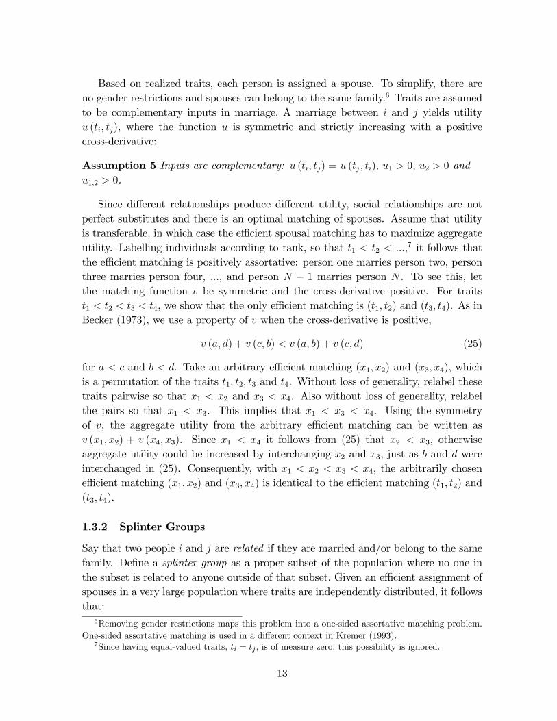
Based on realized traits, each person is assigned a spouse. To simplify, there areno gender restrictions and spouses can belong to the same family.6 Traits are assumedto be complementary inputs in marriage. A marriage between i and j yields utilityu (ti, tj), where the function u is symmetric and strictly increasing with a positivecross-derivative:

Assumption 5 Inputs are complementary: u (ti, tj) = u (tj, ti), u1 > 0, u2 > 0 andu1,2 > 0.

Since different relationships produce different utility, social relationships are notperfect substitutes and there is an optimal matching of spouses. Assume that utilityis transferable, in which case the effi cient spousal matching has to maximize aggregateutility. Labelling individuals according to rank, so that t1 < t2 < ...,7 it follows thatthe effi cient matching is positively assortative: person one marries person two, personthree marries person four, ..., and person N − 1 marries person N . To see this, letthe matching function v be symmetric and the cross-derivative positive. For traitst1 < t2 < t3 < t4, we show that the only effi cient matching is (t1, t2) and (t3, t4). As inBecker (1973), we use a property of v when the cross-derivative is positive,

v (a, d) + v (c, b) < v (a, b) + v (c, d) (25)

for a < c and b < d. Take an arbitrary effi cient matching (x1, x2) and (x3, x4), whichis a permutation of the traits t1, t2, t3 and t4. Without loss of generality, relabel thesetraits pairwise so that x1 < x2 and x3 < x4. Also without loss of generality, relabelthe pairs so that x1 < x3. This implies that x1 < x3 < x4. Using the symmetryof v, the aggregate utility from the arbitrary effi cient matching can be written asv (x1, x2) + v (x4, x3). Since x1 < x4 it follows from (25) that x2 < x3, otherwiseaggregate utility could be increased by interchanging x2 and x3, just as b and d wereinterchanged in (25). Consequently, with x1 < x2 < x3 < x4, the arbitrarily choseneffi cient matching (x1, x2) and (x3, x4) is identical to the effi cient matching (t1, t2) and(t3, t4).

1.3.2 Splinter Groups

Say that two people i and j are related if they are married and/or belong to the samefamily. Define a splinter group as a proper subset of the population where no one inthe subset is related to anyone outside of that subset. Given an effi cient assignment ofspouses in a very large population where traits are independently distributed, it followsthat:

6Removing gender restrictions maps this problem into a one-sided assortative matching problem.One-sided assortative matching is used in a different context in Kremer (1993).

7Since having equal-valued traits, ti = tj , is of measure zero, this possibility is ignored.

13

Proposition 5 The probability that splinter groups exist is zero.

Proof: Define a d-regular multigraph with loops, where every vertex corresponds toa family, and every edge corresponds to a marriage. A splinter group is equivalent toan unconnected component of this graph. Assortative marriages on independent traitsgenerate a random configuration of vertices. A random configuration is equivalent toa regular random multigraph, as defined in Janson et al. (2000). A regular randommultigraph is asymptotically almost surely Hamilitonian for d > 3 (Janson et al. 2000).Connectivity follows from Hamiltonicity, which rules out the existence of unconnectedcomponents, and consequently, the existence of splinter groups. �A partial explanation for this result is that if person imarries person j, then because

of the independence of traits, it is unlikely that anyone else in i’s family marries intoj’s family as well. As the population grows larger, it becomes less and less likely thatthere is more than one marriage between the families of i and j. This “mismatch”prevents i and j, and their families, from socially isolating themselves from the largerpopulation. The problem is more interesting than what this partial intuition conveys,however. The likelihood of more than one marriage between two particular familiesdecreases as the population grows larger, but on the other hand, the number of familiesfor whom this event could occur increases. If, for example, d had been equal to two,then these two effects would have balanced, so that small splinter groups would haveformed even as the population approached infinity. This proof most likely also goesthrough for d ≥ 3, since it really only needs connectivity and since connectivity isclosely related to cubic graphs. The fourth edge is necessary in the case of multigraphsto ensure Hamiltonicity, but Hamiltonicity is stronger than connectivity.In addition to the above proof, we can provide a more structured intuition for no

splinter groups by using a branching tree to trace out relationships in the population.Let Σ be the set of all families. Define an arbitrary family in Σ as the singleton setσ (0). Let σ (1) be the set of families in Σ/σ (0) with at least one family membermarried to someone in the original family σ (0). Define σ (2) as the set of families inΣ/ (σ (0) ∪ σ (1)) with at least one family member married to someone in σ (1). Con-tinuing by iteration to more and more distant relations, let σ (r) be the set of familiesin Σ/ (σ (r − 2) ∪ σ (r − 1)) married to someone in σ (r − 1). The variable r denoteswhat is sometimes called the degree of separation between the initial family σ (0) andthe families in σ (r). The degree of separation is a measure of the social distance be-tween individuals; compare Milgram (1967). The collection of these sets, ∪rq=0 σ (q),constitutes a branching tree. The sets in this collection are mutually exclusive, but ifthere are splinter groups, the sets are not exhaustive even as r →∞. Denote by s (r)

the cardinality of the set σ (r). Since each family in σ (r) is composed of d family mem-bers, where at least one member in each family by definition is married into σ (r − 1),

14

the expansion of the tree ∪rq=0 σ (q) is bounded by

s (r + 1) ≤ s (r) (d− 1) . (26)

If equation (26) holds with equality, then as r increases s (r) very soon encompassesthe entire population. It turns out that the equation generally holds as an inequality,however. The reason for this slowdown is threefold. First, a person in σ (r) could marryanother person in σ (r). Second, a family in σ (r) could have more than one familymember married to someone in σ (r − 1). Thirdly, several people in σ (r) could marryinto the same family. These three types of events combine to prevent each family inσ (r) from contributing a full d − 1 new families to σ (r + 1), and consequently cause(26) to hold as an inequality.Applying the branching tree ∪rq=0 σ (q) to the effi cient assortative matching, the

branching tree is overwhelmingly likely to grow to encompass the entire population inthe limit. Since the branching tree only expands to include people who are directlyor indirectly related, this limit result is equivalent to Proposition 5 that there are nosplinter groups. To see why the entire population is included in the limit, consider whatwould happen if it were not true, if the branching tree died out without having reacheda positive fraction of the population. If this were the case, then σ (r) would eventuallyhave to grow arbitrarily small relative to the remainder set Σ/ (σ (r − 2) ∪ σ (r − 1)),and therefore the likelihood that someone in σ (r) married someone else in σ (r) ratherthan in the remainder set, or that several people in σ (r − 1) married into the samefamily in σ (r) rather than in the remainder set, or that several people in σ (r) marriedinto the same family in the remainder set, must also grow arbitrarily small. But thenequation (26) should hold as an equality, implying that s (r + 1) > s (r), which contra-dicts the premise that the branching tree died out without having reached the entirepopulation. Consequently, everyone in the population is either directly or indirectlyrelated, and there are no splinter groups.

1.3.3 Implications for Productivity

The social network developed here allows more individual choice than the random in-teraction model analyzed earlier, since here industry choice can be made contingenton every aspect of the social structure. The main results from the random interactionmodel continue to hold nevertheless. A large group cannot align social relationships soas to maximize productivity in a small industry where social interaction and produc-tivity are complementary, without incurring the cost of deteriorating social matchesthat comes from breaking up into smaller groups. This follows from the result that nosplinter groups arise under first-best matching on social traits. Since the social choiceset of ethnic minority groups is restricted anyway, these groups can limit their social

15

interactions to a single industry at no alternative cost. Ethnic minorities are thereforewell suited for social interaction-intensive industries.A social network with the same properties could also be derived from a meeting

technology where spouses meet and marry at random. The social structure derivedhere can therefore equally well be thought of as arising in a rigid environment wherepeople meet randomly, as arising from effi cient matching. Since randomness is likely toplay a role in who marries whom, this adds additional strength to the result. Breakingup into smaller groups does not only carry a social utility cost, but also carries the costof bypassing random marriages.

1.3.4 Future Model Extensions

An interesting extension for future work is to include both general and specific skillsin the same framework. In such a model of spillovers between sectors, it should bepossible to derive stratification in overall entrepreneurial activity as well as industrystratification between different forms of self-employed entrepreneurship at the sametime. This would correspond to the current situation in the United States, wheregroups like the Koreans are strongly clustered in a few business sectors, while at thesame time being overrepresented as self-employed owners in almost all other businessactivities as well.

2 Empirical Appendix: Earnings Estimations

Our model makes an additional prediction that members of an ethnic group can achievegreater earnings when entering a common entrepreneurial setting. In our framework,social complementarities produce a positive relationship between earnings and entre-preneurship at the group level. This prediction is in direct contrast to what wouldbe expected if discrimination in the marketplace is the most important factor leadingto segmented group self-employment. The empirical work of Patel and Vella (2013)strongly shows a positive earning relationship for immigrant groups and common groupoccupational choices using the 1980-2000 Census of Populations data. To close the loopfor this paper, we thus provide a brief analysis of earnings and refer readers to thesecomplementary pieces for additional evidence.Table A2 provides individual-level estimations of the earnings relationship. The

outcome variable is the log yearly income of individuals. The core regressors, which wefurther describe shortly, measure the entrepreneurial activity of the individual’s ethnicgroup and whether the individual is self-employed. The sample is taken from the 2000Census IPUMS. We include males aged 30-65 in 2000. Our sample contains all nativemales and immigrant males who migrate after 1968 (effective date of the ImmigrationReform Act of 1965) and have lived in the United States for at least 10 years. The

16

sample excludes workers whose self-employment status is unknown or not applicable,industries without self-employment, and workers living outside of metropolitan areas.We report three core explanatory variables. The first is whether the individual

is self-employed. The second is the percentage of an individual’s ethnic group whoare self-employed (similar to the values reported in Table 1a), regardless of industry.Third, we measure the share of the individual’s ethnic group that is employed in theindustry of the focal individual. With the model developed, we anticipate both of thesegroup measures to have positive predictive power. For natives, these latter variablesare simply measured over the whole US-born population.Our estimations also include many unreported controls for individuals that relate to

earnings. We include fixed effects for PUMA geographical locations and for industries.We also control for high-school and college education, whether the individual is a nativeor an immigrant, whether the individual is fluent in the English language, and fixedeffects for seven age categories and seven age-at-immigration categories. Regressionscluster standard errors by ethnic group and use IPUMS sample weights.The first three columns show that all three elements are predictive of earnings.

Being self-employed (a binary measure) is directly associated with a 3% increase in totalearnings in the cross-section. A 1% increase in the rate of overall self-employment foran ethnic group connects to a 1% increase in total earnings. To aid interpretation, thebottom of the table also provides the standard deviation x beta coeffi cient for group-level variables; a one standard-deviation increase (0.0255) in group self-employmentconnects to 3% higher earning. Similarly, looking at ethnic group concentration for theindividual in his particular industry, a 1% increase in group concentration connects toa 0.6% increase in total earnings. In standard-deviation terms, the relative effect of5% is even larger than the 3% for group self-employment. Columns 4-6 show similaroutcomes when we exclude workers in professional occupations and holders of doctoratedegrees.These results thus support the model’s structure. They also signal for immigrant

groups a potential positive benefit from entrepreneurial concentration. We note, how-ever, that this analysis and the connected empirical work of Patel and Vella (2013) arejust first steps toward understanding this complex and important set of relationships.We particularly believe it is important for future theoretical and empirical work toconsider both owners and employees of firms. Empirical work can particularly targetemployer-employee datasets to observe more detailed hiring and wage patterns; suchwork can also evaluate job transitions during the assimilation of new members of ethnicgroups, perhaps ultimately leading to starting their own business.

17

3 Additional Appendix References:

Heckman, James and Bo Honore. 1990. The empirical content of the Roy model.Econometrica 58: 1121-1149.

Jackson, Matthew, and Asher Wolinsky. 1996. A strategic model of social and economicnetworks. Journal of Economic Theory 71: 44-74.

Janson, Svante, Tomasz Luczak, and Andrzej Rucinski. 2000. Random Graphs. NewYork: John Wiley.

Kremer, Michael. 1993. The O-ring theory of economic development. Quarterly Jour-nal of Economics 108: 551-575.

Milgram, Stanley. 1967. The small world problem. Psychology Today 22: 61-67.

18

X

θ (X)

A

BU

X

θ (X)

A

BU

Figure A1. Individual productivity and the three stationary equilibria: one specialized equilibrium with minority specialization (A), one specialized equilibrium with majority specialization (B), and one unstratified equilibrium (U).

Xt+1 X* X t+2 X t X

p t+1

pt+2

θ (X)

Xt+1 X* X t+2 X t X

p t+1

pt+2

θ (X)

Figure A2. Stable dynamics when the internal effect dominates.

0 a b 1 X

q(X,X)

q(b,X)

q(a,X)

0 a b 1 X

q(X,X)

q(b,X)

q(a,X)

Figure A3. Sorting versus interaction effects in individual productivity. The dotted lines illustrate how the interaction effect raises productivity at all ability levels when specialization increases from a to b. The solid line shows the productivity of the marginal entrepreneur, for whom i=X at every level of X.

μ(XA) - μ(XB)p0

0

V(1,0) v* V(0,1) v

μ(XA) - μ(XB)p0

0

V(1,0) v* V(0,1) v

Figure A4. The difference in mean earnings between group A and group B, for different values of v, when minority group A specializes.

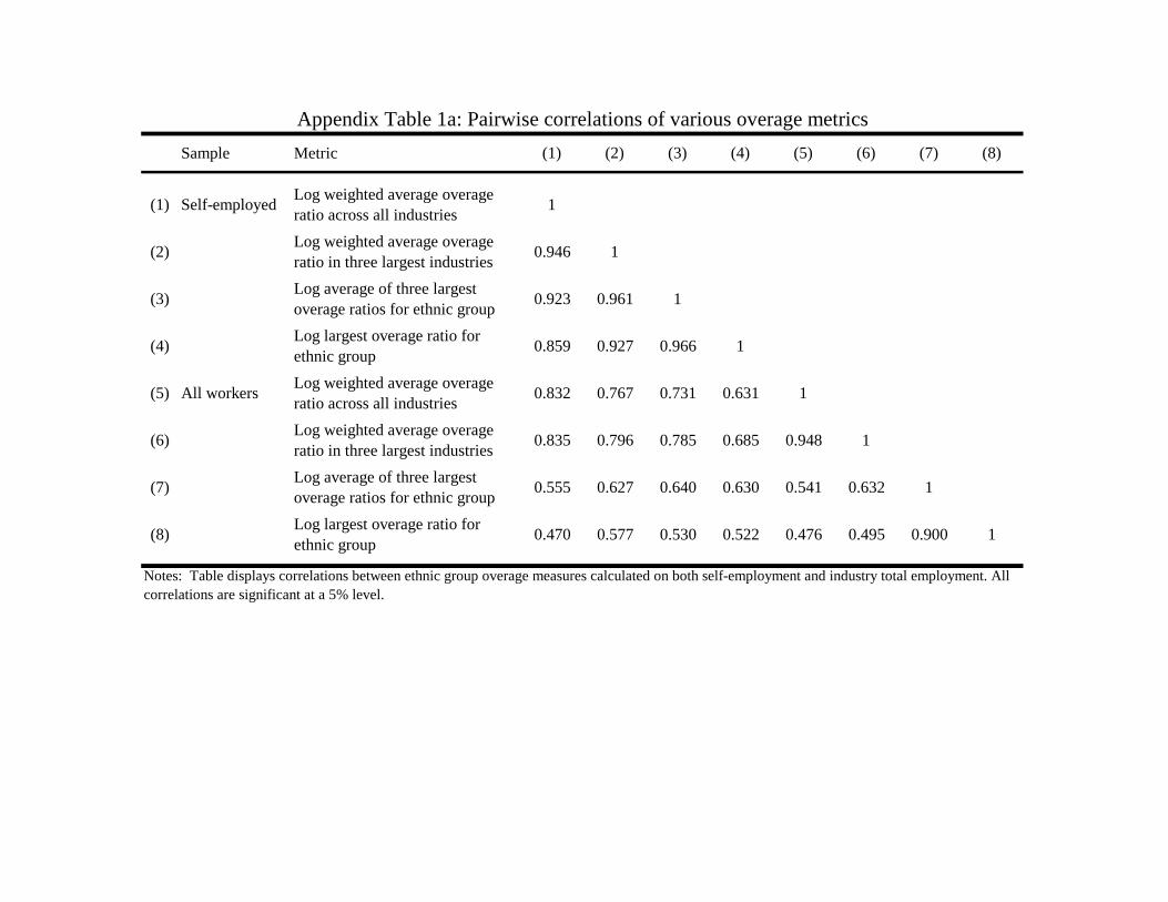
Sample Metric (1) (2) (3) (4) (5) (6) (7) (8)

(1) Self-employed Log weighted average overageratio across all industries 1

(2) Log weighted average overage ratio in three largest industries 0.946 1

(3) Log average of three largest overage ratios for ethnic group 0.923 0.961 1

(4) Log largest overage ratio for ethnic group 0.859 0.927 0.966 1

(5) All workers Log weighted average overage ratio across all industries 0.832 0.767 0.731 0.631 1

(6) Log weighted average overage ratio in three largest industries 0.835 0.796 0.785 0.685 0.948 1

(7) Log average of three largest overage ratios for ethnic group 0.555 0.627 0.640 0.630 0.541 0.632 1

(8) Log largest overage ratio for ethnic group 0.470 0.577 0.530 0.522 0.476 0.495 0.900 1

Appendix Table 1a: Pairwise correlations of various overage metrics

Notes: Table displays correlations between ethnic group overage measures calculated on both self-employment and industry total employment. All correlations are significant at a 5% level.

Sample Metric (1) (2) (3) (4) (5) (6) (7) (8)

(1) Self-employed Log weighted average overage ratio across all industries 1

(2) Log weighted average overage ratio in three largest industries 0.808 1

(3) Log average of three largest overage ratios for ethnic group 0.588 0.789 1

(4) Log largest overage ratio for ethnic group 0.569 0.760 0.971 1

(5) All workers Log weighted average overage ratio across all industries 0.835 0.821 0.661 0.648 1

(6) Log weighted average overage ratio in three largest industries 0.706 0.859 0.719 0.678 0.872 1

(7) Log average of three largest overage ratios for ethnic group 0.589 0.739 0.768 0.816 0.760 0.743 1

(8) Log largest overage ratio for ethnic group 0.587 0.705 0.705 0.742 0.749 0.724 0.955 1

Appendix Table 1b: Pairwise rank correlations of various overage metrics

Notes: See Appendix Table 1a. Table displays rank correlations between ethnic group overage measures calculated on both self-employment and industry total employment. All correlations are significant at a 5% level.

(1) (2) (3) (4) (5) (6)

Percent of self-employed in 1.145 1.122 1.091 1.067individual's ethnic group (1) (0.334) (0.335) (0.347) (0.349)

Share of group that is working in 0.680 0.615 0.624 0.562an individual's industry (2) (0.205) (0.201) (0.210) (0.208)

Indicator for individual being 0.031 0.033 0.030 0.022 0.025 0.022self-employed (0.002) (0.004) (0.002) (0.002) (0.004) (0.002)

Observations 1,560,890 1,560,890 1,560,890 1,286,318 1,286,318 1,286,3181 SD change x beta (1) 0.029 0.029 0.028 0.0271 SD change x beta (2) 0.055 0.050 0.050 0.046

Table A2: Estimations for log yearly income of individual

Notes: Estimations describe the OLS relationship between log yearly income of individuals and entrepreneurial activity of their ethnic group. Sample is taken from 2000 Census IPUMS. Sample includes native males and immigrant males who migrate after 1968 (effective date of the Immigration Reform Act of 1965), are aged 30-65 in 2000, and have lived in the United States for at least 10 years. Sample excludes workers whose self-employment status is unknown or not applicable, industries without self-employment, and workers living outside of metropolitan areas. Baseline estimation includes fixed effects for the following person-level traits (category counts in parentheses): PUMA geographical location (625), industry (200), native/immigrant (2), age (7), age at immigration for migrants (7), education (3), and English language fluency (2). Regressions cluster standard errors by ethnic group and use IPUMS sample weights. The bottom of the table provides the standard deviation x beta coefficient for the group-level variables (0.0255 for (1), 0.0810 for (2)). Columns 4-6 exclude workers in professional occupations and holders of doctorate degrees.

Baseline estimation Excluding professionals and PhDs