Embed Size (px)
Citation preview
Master in Computing
Master of Science Thesis
Social Crowd Controllers using Reinforcement Learning Methods.
Luiselena Casadiego Bastidas.
Advisor: Nuria Pelechano.
July, 2014.
Abstract
Crowd Simulation is an area of research that is present in several disciplines andindustries. Even though the visualization of crowds is an important subject, thebehavior behind it helps to make it believable. Behavioral modeling can be a te-dious task because the agents have to mimic the complexity of human reactions tosituations. In this work, we propose an alternative model for crowd simulation ofpedestrian movements using Reinforcement Learning methods for low level deci-sions. Taking the approach of microscopic models, we trained an agent to reach agoal point while avoiding obstacles that might be on its way, and trying to follow acoherent path during the walk. Once one agent has learned, its knowledge is passedto the rest of the members of the crowd by sharing the resulting Q-Table, expectingthe individual behavior and interactions to lead to a crowd behavior. We presentedstates sets, an action set and reward functions general enough to adapt to differentenvironments, allowing us to use the same knowledge in different scenario settings.
Contents
1 Introduction 11.1 Introduction . . . . . . . . . . . . . . . . . . . . . . . . . . . . . . . . . . 11.2 Objectives . . . . . . . . . . . . . . . . . . . . . . . . . . . . . . . . . . . 31.3 Motivation . . . . . . . . . . . . . . . . . . . . . . . . . . . . . . . . . . . 31.4 Organization . . . . . . . . . . . . . . . . . . . . . . . . . . . . . . . . . . 4
2 State of the Art 52.1 Social Force Models . . . . . . . . . . . . . . . . . . . . . . . . . . . . . . 52.2 Cellular Automata Models . . . . . . . . . . . . . . . . . . . . . . . . . . 62.3 Rule-Based Models . . . . . . . . . . . . . . . . . . . . . . . . . . . . . . 72.4 Reinforcement Learning . . . . . . . . . . . . . . . . . . . . . . . . . . . 8
2.4.1 Elements of Reinforcement Learning . . . . . . . . . . . . . . . . 92.4.2 The Agent-Environment Interface . . . . . . . . . . . . . . . . . 102.4.3 Setting goals and how to achieve them . . . . . . . . . . . . . . . 112.4.4 Markov Decision Processes (MDP) . . . . . . . . . . . . . . . . . 132.4.5 Value Functions . . . . . . . . . . . . . . . . . . . . . . . . . . . . 142.4.6 Related Work . . . . . . . . . . . . . . . . . . . . . . . . . . . . . 16
3 Our Approach 203.1 Crowd Controller Module . . . . . . . . . . . . . . . . . . . . . . . . . . . 233.2 Reinforcement Learning Module . . . . . . . . . . . . . . . . . . . . . . 25
3.2.1 Reinforcement Learning Library . . . . . . . . . . . . . . . . . . 273.2.2 Learning Problem definition. . . . . . . . . . . . . . . . . . . . . 29
3.2.2.1 State definition . . . . . . . . . . . . . . . . . . . . . . . 303.2.2.2 Action definition . . . . . . . . . . . . . . . . . . . . . . 363.2.2.3 Reward function . . . . . . . . . . . . . . . . . . . . . . 37
3.3 Specifications of our experiment setup. . . . . . . . . . . . . . . . . . . . 41
CONTENTS
4 Results 424.1 Evaluation of the reward function. . . . . . . . . . . . . . . . . . . . . . 42
4.1.1 Training Process . . . . . . . . . . . . . . . . . . . . . . . . . . . 444.1.2 Demo Simulation . . . . . . . . . . . . . . . . . . . . . . . . . . . 47
4.2 The second states set approach . . . . . . . . . . . . . . . . . . . . . . . 514.3 Visual results. . . . . . . . . . . . . . . . . . . . . . . . . . . . . . . . . . 55
5 Conclusions 645.1 Conclusions . . . . . . . . . . . . . . . . . . . . . . . . . . . . . . . . . . 645.2 Future Work . . . . . . . . . . . . . . . . . . . . . . . . . . . . . . . . . . 65
List of Figures
2.1 The agent-environment interaction in reinforcement learning. . . . . . 102.2 Backup diagrams for (a) V πand (b) Qπ. . . . . . . . . . . . . . . . . . . . 16
3.1 Q-table example . . . . . . . . . . . . . . . . . . . . . . . . . . . . . . . . 213.2 Modules relationship . . . . . . . . . . . . . . . . . . . . . . . . . . . . . 233.3 Communications chart between modules . . . . . . . . . . . . . . . . . 263.4 Composition of States . . . . . . . . . . . . . . . . . . . . . . . . . . . . 313.5 Goal State Definition . . . . . . . . . . . . . . . . . . . . . . . . . . . . . 323.6 Obstacle State Definition . . . . . . . . . . . . . . . . . . . . . . . . . . . 333.7 Distance State Definition . . . . . . . . . . . . . . . . . . . . . . . . . . . 333.8 Change in Obstacle State definition . . . . . . . . . . . . . . . . . . . . 353.9 Occupancy Code . . . . . . . . . . . . . . . . . . . . . . . . . . . . . . . . 353.10 Description of movements: (a) King’s movements (b) Action definition
by rotation of orientation vector . . . . . . . . . . . . . . . . . . . . . . . 373.11 Distance Gain: (a) Direction Vector to the goal in t-1 and t, (b) Cases
of distance gain. . . . . . . . . . . . . . . . . . . . . . . . . . . . . . . . 393.12 Reward by Cosine: (a) Direction Vector to the goal and Agent’s direc-
tion vector, (b) Some of the reward values for certain angles . . . . . . 40
4.1 Reward Function Evaluation: Tests Setting . . . . . . . . . . . . . . . . 434.2 Ratio of Distance Gained per step during training process. . . . . . . . 454.3 Ratio of Path followed for Distance Gained during training process. . 454.4 Rate of success during training process . . . . . . . . . . . . . . . . . . 464.5 Rate of collisions during training process . . . . . . . . . . . . . . . . . 464.6 Ratio of Distance Gained per step during demo simulation. . . . . . . . 474.7 Ratio of Path followed for Distance Gained during demo simulation. . 484.8 Rate of success during demo simulation. . . . . . . . . . . . . . . . . . . 48

LIST OF FIGURES
4.9 Rate of collisions during demo simulation. . . . . . . . . . . . . . . . . 494.10 Results of simulation on an environment without obstacle. . . . . . . . 504.11 Ratio of Distance Gained per step during simulation without an ob-
stacle. . . . . . . . . . . . . . . . . . . . . . . . . . . . . . . . . . . . . . . 504.12 Ratio of Path taken for Distance Gained during simulation without
an obstacle. . . . . . . . . . . . . . . . . . . . . . . . . . . . . . . . . . . 514.13 Same state definition for different situations . . . . . . . . . . . . . . . 524.14 Twins Test for first state set approach . . . . . . . . . . . . . . . . . . . 524.15 (a) First state set approach vs (b) Second state set approach . . . . . . 534.16 Second state set approach twins test: (a) Overlapping obstacles, (b)
Close obstacles, (c) Not enough space for the agent to walk throughand (d) Tight fit for the agent to walk through. . . . . . . . . . . . . . . 54
4.17 Single agent in field of dummies. . . . . . . . . . . . . . . . . . . . . . . 554.18 Six agents in circle crossing. . . . . . . . . . . . . . . . . . . . . . . . . . 564.19 Six agents in circle crossing with an obstacle in the middle. . . . . . . . 574.20 Six agents in line crossing. . . . . . . . . . . . . . . . . . . . . . . . . . . 584.21 Six agents in line crossing with a moving obstacle. . . . . . . . . . . . . 594.22 Six agents reaching for the same goal. . . . . . . . . . . . . . . . . . . . 604.23 Six agents reaching for the same goal with a moving obstacle. . . . . . 614.24 Best case scenario for a simulation of 12 agents in circle. . . . . . . . . 624.25 Worst case scenario for a simulation of 12 agents in circle. . . . . . . . 63

Chapter 1
Introduction
1.1 Introduction
Crowd Simulation is an area that has experienced significant development in thesepast few decades. The use of virtual crowds is not restrained to the scientific field,they are so versatile that, they can be found in the entertainment industry an ad-vertisement as well. Crowd simulation is a key component to research experimentsor products where the use of a large amount of “actors” is not feasible or safe. Pro-vides a way to study the behavior of a collection of individuals under specific cir-cumstances and an alternative to populate scenarios with control over them, stillportraying believable or coherent responses to the environment and themselves.
The task of producing a virtual crowd is not a simple one. There are two mainissues to take into account: the behavioral aspect and the visualization [1]. Theweight of importance given to these problems are defined by the type of applicationthe virtual crowd is going to be a part of. If the purpose of the application is tostudy the reaction of crowds under certain circumstances (like evacuation underhazard or navigation through crowded rooms) the visualization of the individualsas characters might be discarded. Results can be appreciated with the use of dotsor simpler figures. In the other case, if the goal is to produce virtual crowds to fill orpopulate scenarios (like movies, commercials and games) it is imperative to work ina high quality visual representation of these characters. Either way, compromisingone aspect for the other leaves us with results that are not the most convincing.Having a group of dots moving around doesn’t give us a sense of crowd nor doesa group of characters going through walls and each other. A virtual crowd should
1
CHAPTER 1. INTRODUCTION 2
have the balance between looking good and behaving in a believable manner.
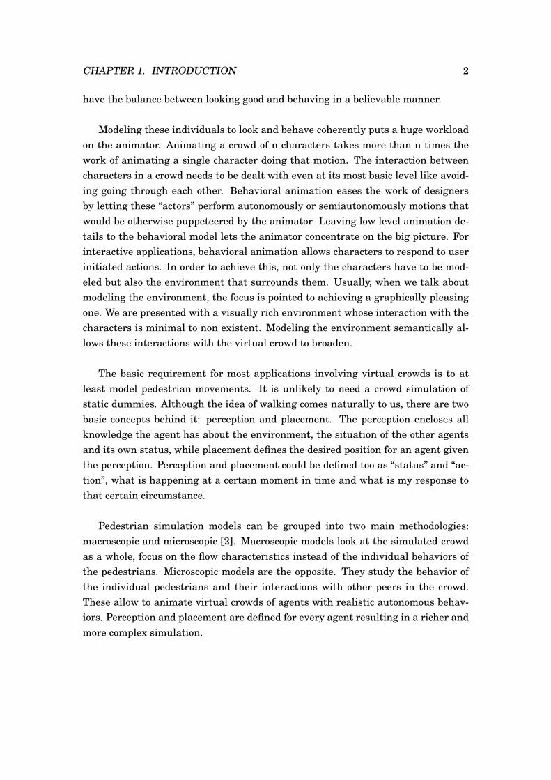
Modeling these individuals to look and behave coherently puts a huge workloadon the animator. Animating a crowd of n characters takes more than n times thework of animating a single character doing that motion. The interaction betweencharacters in a crowd needs to be dealt with even at its most basic level like avoid-ing going through each other. Behavioral animation eases the work of designersby letting these “actors” perform autonomously or semiautonomously motions thatwould be otherwise puppeteered by the animator. Leaving low level animation de-tails to the behavioral model lets the animator concentrate on the big picture. Forinteractive applications, behavioral animation allows characters to respond to userinitiated actions. In order to achieve this, not only the characters have to be mod-eled but also the environment that surrounds them. Usually, when we talk aboutmodeling the environment, the focus is pointed to achieving a graphically pleasingone. We are presented with a visually rich environment whose interaction with thecharacters is minimal to non existent. Modeling the environment semantically al-lows these interactions with the virtual crowd to broaden.
The basic requirement for most applications involving virtual crowds is to atleast model pedestrian movements. It is unlikely to need a crowd simulation ofstatic dummies. Although the idea of walking comes naturally to us, there are twobasic concepts behind it: perception and placement. The perception encloses allknowledge the agent has about the environment, the situation of the other agentsand its own status, while placement defines the desired position for an agent giventhe perception. Perception and placement could be defined too as “status” and “ac-tion”, what is happening at a certain moment in time and what is my response tothat certain circumstance.
Pedestrian simulation models can be grouped into two main methodologies:macroscopic and microscopic [2]. Macroscopic models look at the simulated crowdas a whole, focus on the flow characteristics instead of the individual behaviors ofthe pedestrians. Microscopic models are the opposite. They study the behavior ofthe individual pedestrians and their interactions with other peers in the crowd.These allow to animate virtual crowds of agents with realistic autonomous behav-iors. Perception and placement are defined for every agent resulting in a richer andmore complex simulation.
CHAPTER 1. INTRODUCTION 3
In the state of the art for microscopic methods such as Rule-Based models, Cel-lular Automata models and Social Force models, the agent is instructed, in a wayor another, what to do when faced with certain circumstances. We do get an au-tonomous agent but its intelligence comes from what it was taught to be good andbad. Reinforcement Learning is a learning method that has been around for manyyears now in the areas of Artificial Intelligence and Robotics. This method allowsthe agent to learn from experience with the environment what it should be aimingfor and what should be avoided, all this by maximizing a reward signal given by theenvironment itself on what repercussion his action choice brought.
In this work we would like to present Reinforcement Learning methods as avalid alternative to known pedestrian microscopic models for low level decisions.
1.2 Objectives
Our main goal with this work is to present a coherently functional crowd sim-ulation of autonomous agents using the Reinforcement Learning Model. Toachieve this, we have set a series of stepping stones to conquer:
• Model the perception of the environment in a general way.
• Define actions simple enough to work in several settings.
• Calibrate the reward function of the different perceptions of the environment.
In our final case scenario, the agents should be able to: avoid going through obsta-cles, avoid collision with their peers and obstacles and reach their goal. All of theseby following a natural and logical route through the environment.
1.3 Motivation
Our motivation of working with Reinforcement Learning in Crowd Simulation comesfrom the need to ease the workload inherent on it. Our premise is that once an agentknows how to behave individually, the interaction with other agents with the sameknowledge will result in a coherent crowd behavior on a shared environment. TheReinforcement Learning model can be adapted to portray the two basic elementsof pedestrian movements that are perception and placement, where the transition
CHAPTER 1. INTRODUCTION 4
from a place to another comes from the valued experience the agent has for thatchange. The RL model allows us to abstract from a prestablished environment bymodeling situations (states) that could be present in any configuration of this one.The independence of a setting makes this approach appealing to us, because theagent can adapt its knowledge to the new scenarios it is presented with and refineit by experiencing with this new world.
1.4 Organization
After the introduction and definition of our objectives, we proceed to make a briefsummary on the main methodologies to model pedestrian movements and some ofthe most recent approaches in the State of the Art. Then comes the theoreticalexplanation of the methodology we used in the next chapter, continuing to the prac-tical side of what we present as an alternative to the already known approachesin Technical Development. Lastly we present the results of our different scenariosand the conclusions we reached in the last two chapters.

Chapter 2
State of the Art
In this chapter we discuss the three most used microscopic approaches to modelpedestrian movements and the most recent works employing them. Then we intro-duce the Reinforcement Learning method defining its most important concepts andthe overall process of how it works [2, 3] , ending that section with some relatedworks in the area of Crowd Simulation that have used this method.
2.1 Social Force Models
The social force model was first presented in [4], they establish that the motion ofpedestrians can be described as if they would be subjected to “social forces”. Thesevirtual forces are analogous to real forces like repulsive interaction, friction forces,dissipation and fluctuations. Each force parameter has a natural interpretation,is individual for each pedestrian, and is often chosen randomly within some em-pirically found or otherwise plausible interval. Social forces model human crowdbehavior with a mixture of physical and sociopsychological factors. This model ap-plies repulsion and tangential forces to simulate the interaction between people andobstacles, allowing a realistic “pushing” behavior and variable flow rates.
In 2010, Moussaid et.al [5] used a social forces model to study the impact of thewalking behavior of groups in the crowd dynamics. Shukla [6] extended it to includeimproved velocity-dependent interaction forces, this allows to consider interactionsof pedestrians with both static and dynamic obstacles.
In 2011, Dutra et.al [7] used a social forces model on their hybrid model for
5
CHAPTER 2. STATE OF THE ART 6
crowd simulation, to prevent collisions between agents and, between agents andobstacles. Saboia and Goldenstein [8] , proposed the use of lattice-gas concepts onthe social force model to reduce artifacts when there is low density of pedestrians.Zanlungo et al. [9] introduced a new specification of the social force model in whichpedestrians explicitly predict the place and time of the next collision in order toavoid it. Similarly in 2013, Gao et al. [10] worked on a modified social force modelthat considers relative velocity to enhance the realism of the simulation.
In 2012, Yan et al. [11] proposed a novel swarm optimization based on socialforces model (SFSO). Later in the year, Li and Jiang [12] presented a novel frictionbased social force model that allowed to focus on the individual initiative.
Finally in 2013, an evacuation model is proposed by Jiahui et al. [13] to optimizethe social force model by taking into account the cohesion among passengers of asubway an the nervousness factor in an emergency.
2.2 Cellular Automata Models
Cellular Automata is an artificial intelligence approach to simulation modeling de-fined as mathematical idealizations of physical systems, in which space and timeare discrete, and physical quantities take a finite set of discrete values. The space isrepresented as an uniform lattice of cells with local states subject to a uniform setof rules, which drives the behavior of the system. These rules compute the state of aparticular cell as a function of its previous state and the states of the adjacent cells[14]. CA models do not allow contact between agents, floor space is discrete andindividuals can only move to an adjacent free cell. This approach offers realistic re-sults for lower density crowds, but unrealistic results when agents in high-densitysituations are forced into discreet cells.
In 2010, Sarmady et al. [15] presented a new approach of finer grid cellularautomata, thought to alleviate the problem of the chess like movements witnessedin traditional cellular automata models. Then in 2011, Zhang et al. [16] proposeda simulation model of pedestrian flow based on geographical cellular automata.Zhiqiang et al. [17] improved and optimized a traditional discrete cellular automatafor a crowd evacuation model of a supermarket. Long et al. [18] worked on a modifi-cation to the traditional cellular automata, aiming to take into account abandoned
CHAPTER 2. STATE OF THE ART 7
possessions and luggage on an emergency evacuation of a passenger station.
In 2012, Zainuddin and Aik [19] presented a cellular automata model to simu-late the circular movements of Muslim pilgrims performing the Tawaf ritual withinthe Masjid Al-haram facility in Makkah. They tackled the issue of circular motionsin Cellular Automata, that so far, had not been too explored; and they took intoaccount the pedestrian’s ability to select the exit route.
In 2013, Carneiro et al. [20] proposed a model that uses 2d cellular automatato simulate the crowd evacuation behavior in a soccer stadium. Ben at.al [21] pre-sented an agent-based modeling approach in the cellular automata environmentfor evacuation simulation. Chang worked twice with cellular automata this yearfor personnel evacuation [22, 23], the first time modeling with stochastic cellularautomata located nearest to the exist; and the second time, he modified his modelto base it in a 2.5D cellular automata.
This year, Giitsidis and Sirakoulis [24] presented a simulation for emergencyevacuation of disembarking aircraft employing cellular automata.
2.3 Rule-Based Models
Rule-Based Models are considered by many the first approach in the field of be-havioral animation. Derived from the Reynold’s work in [25], they are based onthe premise that the group behavior is just the result of the interaction betweenthe individual behavior of the group members. Therefore, it would be enough tosimulate simple actions on agents individually and the more complex behavior ofthe crowd would emerge from the interaction between them. These models charac-terize themselves by applying a set of rules over the agents, these rules establishthe response to the situations presented by the environment and what we want theagents to achieve.
In 2010, Xiong et al. [26], worked on a multiagent-based simulation to study thespatial and temporal transmission of HIV/AIDS among injection drug users. Theagents followed behavior rules for: movement, infection, social influence and for thedevelopment of AIDS. Wulansari [27], proposed the same year an implementationof a steering model to simulate a crowd during the tawaf ritual. It evaluates sev-

CHAPTER 2. STATE OF THE ART 8
eral pilgrim’s behaviors like walking on a certain direction, collision avoidance andobstacle avoidance.
In 2011, Kumarage et al. [28], presented a simulation of a hornet attack wherethey used OpenSteer [29] for the simple steering behaviors of their agents. Sunand Qin [30], implemented a model that adopted the rule-based module to generateappropriate behaviors according to event reactions. Yu and Duan [31], modeled anevacuation simulation using rules that defined the movement of the agents duringthe run. Then in 2012, Yuan et al. [32] worked on a method to populate virtual en-vironments with crowd patches, these patches were pre-calculated and reused thecrowd simulation modeled using a rule-based method.
This year, Zhong et al. [33] proposed an evolutionary framework to automati-cally extract decision rules for agent-based crowd models.
2.4 Reinforcement Learning
Reinforcement learning is the learning process where an agent needs to learn whatto do and how to map situation to actions so as to maximize a numerical rewardsignal. The learner is not told which actions to take, but instead it must discoverwhich actions yield the most reward by trying them. These actions may affect notonly the immediate reward but also the next situation and through that, all subse-quent rewards. This approach is defined by characterizing a learning problem andnot the learning method. The basic idea is to capture the most important aspectsof the real problem facing a learning agent, during its interaction with its environ-ment to achieve a certain goal [46]. Such agent must be able to sense the state ofthe environment to some extent and must be able to take actions that affect thestate. It must also have a goal or goals relative to the state of the environment. Theformulation can be summarized in these three aspects: perception, action and goal.
One characteristic that separates Reinforcement Learning from other learningmethods is that there exists an issue of balancing exploration and exploitation of theknowledge. To maximize a reward, the agent must prefer actions that it has triedin the past and found to be effective in producing a reward, but to discover saidactions, it has to try actions that it has not selected before. This trade-off betweenexploration and exploitation is one of the challenges of Reinforcement Learning.
CHAPTER 2. STATE OF THE ART 9
The agent has to exploit what it knows already but it also has to explore in orderto make better action selections in the future. Favoring exploitation could leave uswith a solution that is not the best and the other way around could leave us withan agent that is not goal oriented.
2.4.1 Elements of Reinforcement Learning
Besides the agent and environment, four main subelements can be identified on areinforcement learning system: a policy, a reward function, a value function , andoptionally, a model of the environment.
A policy defines the way the learning agent behaves at a given time. Could bedefined as the mapping from perceived states of the environment to actions to betaken when in those states. In psychology, it would correspond to a set of stimulus-response rules or associations. In some systems the policy can be a simple functionor a lookup table, although in others it may involve extensive computation such asa search process. The policy alone is sufficient to determine behavior.
A reward function defines the goal in a reinforcement learning problem. It mapseach perceived state (or state-action pair) of the environment to a single number,a reward, indicating the inherent desirability of that state. The whole purpose ofthe agent is to maximize the total reward it receives in the long run, so the re-ward function tells the agent what are the good and bad events in a state. Thereward function is a defining feature of the problem and it must be unalterable bythe agent, although it can serve as a basis for changing the policy.
A value function specifies what is good in the long run. The value of a stateis the total amount of reward an agent can expect to accumulate over the futurestarting from that state. Values indicate the long term desirability of states aftertaking into account the states that are likely to follow, and the rewards availablein those states. Without rewards there cannot be values, but the whole purpose ofestimating values is to achieve more reward. The action choices are made takinginto account the states with highest values and not highest rewards, because theseactions will yield us a better amount of reward in the future.
A model of the environment is something that allows us to mimic the behavior

CHAPTER 2. STATE OF THE ART 10
of the environment at any given time. For example, given a state and action, themodel might predict the resultant next state and the next reward, it allows us tomake decisions on a course of action before this has been experienced. Models areused for planning, hence their use is optional depending on the type of applicationthe RL system is going to be used for.
2.4.2 The Agent-Environment Interface
The agent is the learner and the decision maker, the environment is the everythingthat surrounds the agent and what it interacts with. They interact continually, theagent selecting actions and the environment responding to these actions and pre-senting new situations to the agent. The environment is also the responsible forgiving rewards, these numerical values that the agent tries to maximize over time.
The agent and the environment interact at each of a sequence of time steps.At each time step t, the agent receives some representation of the environment’sstate, st ∈ S, where S is the set of possible states, and on that basis selects an ac-tion, at ∈ A(st), where A(st) is the set of actions available in state st. One timestep later, in part as a consequence of its action, the agent receives a numericalreward, rt+1 ∈ R, and finds itself in a new state, st+1. Figure 2.1 diagrams theagent-environment interaction.
Figure 2.1: The agent-environment interaction in reinforcement learning.
At each time step, the agent implements a mapping from states to probabilitiesof selecting each possible action. This mapping is the agent’s policy and is denotedπt, where πt(s, a) is the probability that at = a if st = s. Reinforcement learning

CHAPTER 2. STATE OF THE ART 11
methods specify how the agent modifies its policy as a result of its experience.
The reinforcement learning framework is abstract and flexible. Time steps neednot to refer to fixed intervals of time but could refer to arbitrary successive stages ofdecision-making and acting. Both actions and states can be low-level or high-leveldepending on what the learning problem is to begin with. The states can depicteither physical properties or psychological, they could refer to locations on an envi-ronment, sensorial signals in an agent and even moods perceived. The possibilitiesare endless, as long as, the learning problem can be reduced to three signals pass-ing back an forth between the agent and the environment: one signal to representthe choices made by the agent (actions), one signal to represent the basis on whichthe choices are made (states), and one signal to define the agent’s goal (rewards).
The boundary between what is considered part of the agent and what is consid-ered part of the environment cannot be trivialized to a physical boundary of body vssurroundings. The general rule to follow is that anything that cannot be changedarbitrarily by the agent is considered to be outside of it and thus part of its environ-ment. Also it is not assumed that everything in the environment in unknown to theagent. The agent-environment boundary doesn’t limit the agent’s knowledge but itsabsolute control. In practice, the agent-environment boundary is determined onceone has selected particular states, actions, and rewards, and thus has identified aspecific decision-making task of interest.
2.4.3 Setting goals and how to achieve them
In Reinforcement Learning, the goal of an agent is formalized in terms of a specialreward signal passing from the environment to the agent. At each time steps, thereward is a simple number, rt ∈ R. Informally, the agent’s goal is to maximize thetotal amount of rewards it receives. This mean maximizing not the immediate re-ward but the cumulative reward over time. If we want the agent to do somethingfor us, we must provide rewards to it in such a way that maximizing these rewardsthe agent will also achieve our goal. The reward signal is our way of communicatingto the agent what we want it to achieve.
The ultimate goal of the agent should be something over which it has imperfect

CHAPTER 2. STATE OF THE ART 12
control, it should not be able, for example, to simply decree that the reward hasbeen received in the same way that it might arbitrarily change its action[47].
We have said several times that the agent’s goal is to maximize the reward itreceives in the long run. Formally defined, we seek to maximize the expected return,whereRt is defined as some specific function of the reward sequence rt+1, rt+2, rt+3,...,.In the simplest case, the return is the sum of the rewards:
Rt = rt+1 + rt+2 + rt+3 + ...+ rT , (2.1)
where T is a final time step. This approach makes sense in systems where thereis a natural notion of final time step. When the agent-environment interactionbreaks naturally into subsequences, these are called episodes. Each episode endsin a special state called the terminal state, followed by a reset to a standard start-ing state or to a sample from a standard distribution of starting states. Tasks withepisodes of this kind are called episodic tasks. In some cases, the agent-environmentinteraction does not break naturally into identifiable episodes, but goes on continu-ally without limit. We call these continuing tasks. The return formulation in 2.1 isproblematic for continuing tasks because the final time step would be T = ∞, andthe return, which is what we are trying to maximize, could itself easily be infinite.
To address this, the concept of discounted return is introduced. The agent nowtries to select actions so that the sum of the discounted rewards it receives over thefuture is maximized. The discounted return is defined as:
Rt = rt+1 + γrt+2 + γ2rt+3 + ... =∞∑k=0
γkrt+k+1, (2.2)
where γ is a parameter, 0 ≤ γ ≤ 1, called the discount rate.
The discount rate determines the present value of future rewards: a reward re-ceived k time steps in the future is worth only γk−1 times what it would be worth ifit were received immediately. If γ < 1, the infinite sum has a finite value as long asthe reward sequence {rk} is bounded. If γ = 0, the agent is “nearsighted” in beingconcerned only with maximizing immediate rewards. As γ approaches 1, the objec-tive takes future rewards into account more strongly: the agent becomes farsighted.

CHAPTER 2. STATE OF THE ART 13
2.4.4 Markov Decision Processes (MDP)
In the Reinforcement Learning framework the agent makes its decision as a func-tion of the state. The state is the environment’s signal to the agent, it means what-ever information is available to the agent to make a decision on. Ideally, a state sig-nal should summarize past sensations compactly but in a way that still retains allthe relevant information. A state signal that succeeds in this is said to be Markov,or to have the Markov property. Even if much of the information about the sequencethat led us to the present state were to be lost, a state remains Markov if it repre-sents correctly the result of such sequence over the environment. This is sometimesalso referred as an “independence of path” property because all that matters is inthe current state signal, its meaning is independent of the “path” or history of sig-nals that have led up to it.
To formally define the Markov property, we are going to assume that there area finite number of states and rewards values so this allows us to work in terms ofsums and probabilities. Consider how a general environment might respond at atime t+1 to the action taken at time t. Int he most general causal case, this reponsemay depend on everything that has happened earlier. In this case, the dynamicscan be defines only by specifying the complete probability distribution:
Pr{st+1 = s′, rt+1 = r|st, at, rt, st−1, at−1, ..., r1, s0, a0}, (2.3)
for all s’, r, and all possible values of the past events: st, at, rt, ..., r1, s0, a0. If thestate signal has the Markov property, on the other hand, the environment’s responseat t+1 depends only on the state and action representations at t, in which case theenvironment’s dynamics can be defines by specifying only
Pr{st+1 = s′, rt+1 = r′|st, at}, (2.4)
for all s’, r,st,and at. Meaning, a state signal has the Markov property, and is aMarkov state, if and only if 2.4 is equal to 2.3for all s’,r, and histories,st, at, rt, ..., r1, s0, a0. In this case, the environment and task as a whole are also said to have the Markovproperty. The Markov property is important in reinforcement learning because de-cisions and values are assumed to be functions only of the current state. In order forthese to be effective and informative, the state representation must be informative.

CHAPTER 2. STATE OF THE ART 14
A reinforcement learning task that satisfies the Markov property is called aMarkov decision process, or MDP. If the state and action spaces are finite, then it iscalled a finite Markov decision process (finite MDP). A particular finite MDP is de-fined by its state and action sets and by the one-step dynamics of the environment.Given any state and action, s and a, the probability of each possible next state, s’, is
Pass′ = Pr{st+1 = s′|st = s, at = a}. (2.5)
These quantities are called transition probabilities. Similarly, given any currentstate and action, s and a , together with any next state ,s’, the expected value of thenext reward is
Rass′ = E{rt+1|st = s, at = a, st+1 = s′}. (2.6)
These quantities, Pass′and Rass′ , completely specify the most important aspects ofthe dynamics of a finite MDP.
2.4.5 Value Functions
Most of the reinforcement learning algorithms are based on estimating value func-tions, functions of states (or of state-action pairs) that estimate how good it is forthe agent to be in a given state, or how good it is to perform a given action in a givenstate. This notion of “how good” is defined in terms of expected return. The rewardsthe agent can expect to receive in the future depend on what actions it will take inthe present. In the same way, value functions are defines with respect to particularpolicies.
A policy, π, is a mapping from each state, s ∈ S, and actions, a ∈ A(s), to theprobability, π(s, a) of taking action a when in state s. Informally, the value of a states under the policy π, denoted V π(s), is the expected return when starting in s andfollowing π thereafter. For MDPs, V π(s) can be defined formally as
V π(s) = Eπ{Rt|st = s} = Eπ{∞∑k=0
γkrt+k+1|st = s}, (2.7)
where Eπ{}denotes the expected value given that the agent follows policy π. Thefunction V π is called the state-value function for policy π.
CHAPTER 2. STATE OF THE ART 15
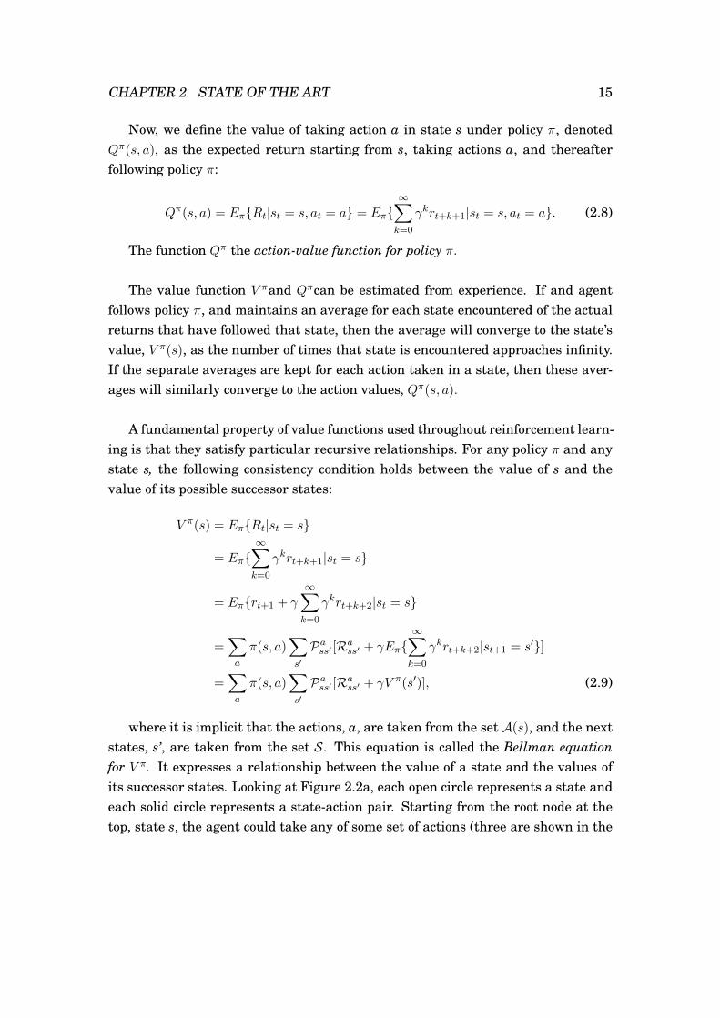
Now, we define the value of taking action a in state s under policy π, denotedQπ(s, a), as the expected return starting from s, taking actions a, and thereafterfollowing policy π:
Qπ(s, a) = Eπ{Rt|st = s, at = a} = Eπ{∞∑k=0
γkrt+k+1|st = s, at = a}. (2.8)
The function Qπ the action-value function for policy π.
The value function V πand Qπcan be estimated from experience. If and agentfollows policy π, and maintains an average for each state encountered of the actualreturns that have followed that state, then the average will converge to the state’svalue, V π(s), as the number of times that state is encountered approaches infinity.If the separate averages are kept for each action taken in a state, then these aver-ages will similarly converge to the action values, Qπ(s, a).
A fundamental property of value functions used throughout reinforcement learn-ing is that they satisfy particular recursive relationships. For any policy π and anystate s, the following consistency condition holds between the value of s and thevalue of its possible successor states:
V π(s) = Eπ{Rt|st = s}
= Eπ{∞∑k=0
γkrt+k+1|st = s}
= Eπ{rt+1 + γ∞∑k=0
γkrt+k+2|st = s}
=∑a
π(s, a)∑s′
Pass′ [Rass′ + γEπ{∞∑k=0
γkrt+k+2|st+1 = s′}]
=∑a
π(s, a)∑s′
Pass′ [Rass′ + γV π(s′)], (2.9)
where it is implicit that the actions, a, are taken from the set A(s), and the nextstates, s’, are taken from the set S. This equation is called the Bellman equationfor V π. It expresses a relationship between the value of a state and the values ofits successor states. Looking at Figure 2.2a, each open circle represents a state andeach solid circle represents a state-action pair. Starting from the root node at thetop, state s, the agent could take any of some set of actions (three are shown in the

CHAPTER 2. STATE OF THE ART 16
figure). From each of these, the environment could respond with one of several nextstates, s’, along with a reward, r. The Bellman equation 2.9 averages over all thepossibilities, weighting each by its probability of occurring. It states that the valueof the start state must equal the (discounted) value of the expected next state, plusthe reward expected along the way.
(a) (b)
Figure 2.2: Backup diagrams for (a) V πand (b) Qπ.
The value function V π is the unique solution to its Bellman equation. Diagramslike the ones shown in Figure 2.2 are called backup diagrams because they diagramrelationships that form the basis for the update or backup operations that are at theheart of reinforcement learning methods. These operation transfer value informa-tion back to a state (or a state-action pair) from its successor states (or state-actionpairs).
2.4.6 Related Work
Reinforcement Learning is slowly gaining some stance in the agent simulation field.Its varied use in the area just shows its real versatility and this method can solvemany learning problems when modeled correctly. Not only is used to model thepedestrian movements as low level decisions but it is implemented for the learningof high level decisions too . In the following works we can see how reinforcementlearning is used to solve some learning problems but approaching them is differentways. The beauty of RL is that its framework can adapt to whatever it is we desireto model, as long as, its elements are defined for such purpose.
In 2010, Torrey [34] proposes reinforcement learning as a viable alternative
CHAPTER 2. STATE OF THE ART 17
method for crowd simulation. Presents a case study of a school domain where theagent’s goal is to reach its designated classroom. She modeled a pretty simple stateset where the agent perceives the time it has left to reach its goal, its distance to itand its distance to the closest other agent. The actions the agent can perform arestaying in the current segment, move one segment towards the goal or move onesegment towards the closest other agent. The agents have two motivations uponwhich they build their rewards: to socialize with other agents and to reach theirgoal classroom. With a small crowd, the results seemed to sustain the initial state-ment but she makes a point of stating the importance of modeling the environment,both state wise and reward wise.
Lee et.al [35] propose a method for inferring the behavior styles of charactercontrollers from a small set of examples. They demonstrate how a rich set of behav-ior variations can be captured by determining the appropriate reward function inthe reinforcement learning framework, and how this can be applied to different en-vironment an scenarios. This approach is based in apprenticeship learning wherean agent learns from an expert agent.
Cuayáhuitl et.al [36] presented an approach for inducing adaptive behavior ofroute instructions. They proposed a two-stage approach to learn a hierarchy ofwayfinding strategies using hierarchical reinforcement learning.Their experimentswere based on an indoor navigation scenario for a building that is complex to navi-gate. Their results showed adaptation to the type of user and structure of the spa-tial environment, plus the learning speed was better than the baseline approachesthey used.
Gil et.al [37] proposed a Q-Learning based multiagent system oriented to pro-vide navigation skills to simulation agents in virtual environments. They focusedon learning local navigation behaviors from the interactions with other agents andthe environment. They adopted and environment-independent state space repre-sentation to provide scalability. Their results showed that RL techniques can beuseful to improve the scalability in the problem of controlling the navigation ofcrowded-oriented agents.
In 2012, Kastanis and Slater [38] used Reinforcement Learning to train a vir-tual character to move participants to a specified location. Based on proxemics
CHAPTER 2. STATE OF THE ART 18
theory, the states for the agent were the four distances from the avatar to the par-ticipant (personal distance, social distance, public distance and not engaged). Theagent had 6 actions that involved walking forward, backwards, stay idle and wave.The reward function was based on the response of the human. If the person movedtowards the target, the agent got a positive reward and in all other cases a negativeone. The results showed that the agent did learn the rule that, when it moves soclose to the participant that it breaks the convention of personal distance, the par-ticipant will tend to move backwards.
Gil et.al [39] presented a calibration method for a framework based in Multi-agent Reinforcement Learning. The agents learned to control individually its in-stant velocity vector in scenarios with collisions and frictions forces. Each agentgets a different learned motion controller. The results indicated similarities in thelearned dynamics of the agents with those of real pedestrians.
In [40], Lo et.al present a novel approach for motion controllers. The agentlearns how to move around evading static obstacles basing its decisions on visioninput. The character “sees” with depth perception skipping this way the manualdesign phase of parametrization state space. They avoid the curse of dimensional-ity by introducing a hierarchical model and a regression algorithm.
In 2013, Rothkopf and Ballard [41] developed a methodology to estimate the rel-ative reward contributions of multiple basic visuomotor tasks to observed naviga-tion behavior using inverse reinforcement learning. The simulations demonstratedthat the reward functions used by the agent that mimics human’s performance onthe task of traversing a walkway with multiple independent goals, can be well re-covered with modest amounts of observation data.
Hao and Leung [42] proposed a social learning framework for a population ofagents to coordinate on socially optimal outcomes in the context of general-sumgames. They used reinforcement learning as a learning strategy instead of evolu-tionary learning. The agents were able to achieve a much more stable coordinationon socially optimal outcomes compared with previous work ,and the framework canbe suitable for both the settings of symmetric and asymmetric games.
Martinez-Gil et al introduce in [43, 44] a multi-agent RL approach for pedestrian
CHAPTER 2. STATE OF THE ART 19
groups where the agents learn to control their velocity, avoid obstacles and otherpedestrians and to reach a goal. They propose a new methodology that uses differ-ent iterative learning strategies, combining a vector quantization with Q-Learningalgorithm. They made comparisons with Helbing’s social force model, obtaining re-sults that validated this approach given the emergence of collective behaviors.
The use Beheshti and Sukthankar [45] gave to reinforcement learning here isdifferent from what we’ve seen so far. They presented this year a reinforcementlearning model for constructing normative agents to model human social systems.The case study was focused on using this architecture to predict trends in smok-ing cessation resulting from a smoke-free campus initiative. The agents learn fromtheir interactions with other agents, their judgment is their reward and a sociallycorrect behavior is learned.
As we can see from these works, RL has been present in the area for someyears now. Its potential is yet to be fully explored, but so far it has been proved togive satisfying results. Our work presents another way of using RL to model lowlevel pedestrian movements, where the agent’s perception is independent from theenvironment overall layout.
Chapter 3
Our Approach
As we saw in the previous chapter, the crowd simulation problem can be approachedfrom different points of view. In the reinforcement learning case, not only we find abroad selection of methods to use, but within these methods, we can still find newways to model the same learning problem (i.e: pedestrian moves), by the variationof the perception of the environment, the actions available to the agent and, mostimportantly, the reward function.
Our approach is based on Q-Learning . Q-learning is a form of model-free rein-forcement learning [48]. Is a simple way for agents to learn how to act optimally incontrolled MDPs. It works by successively improving its evaluations of the qualityof particular actions at particular states. In its simplest form, one-step Q-learningis defined by
Q(st, at)← Q(st, at) + α[rt+1 + γmaxaQ(st+1, a)−Q(st, at)]. (3.1)
In this case, the learned action-value function, Q, directly approximates Q*, theoptimal action-value function, independent of the policy being followed. In 3.1 wecan see the procedural algorithm for Q-Learning.
We will start the learning process of the crowd with just one agent. It will learnhow to walk logically and to reach its goal, while avoiding objects that might be onthe way to it. Once our single agent learns how to fulfill its goals, this knowledgewill be used for the rest of the agents to build knowledge from. Meaning, one willlearn alone the whole task, then this learning will be transferred to the other agentswho will improve it from their own experience. This is possible because, one of the
20
CHAPTER 3. OUR APPROACH 21
Algorithm 3.1 Q-Learning AlgorithmInitialize Q(s,a) arbitrarilyRepeat (for each episode):
Initialize sRepeat(for each step of episode):
Choose a from s using policy derived from Q(e.g.,ε-greedy)Take action a, observe r, s’Q(s, a)← Q(s, a) + α[r + γmaxa′Q(s′, a′)−Q(s− a)]s← s′
until s is terminal
characteristics of Q-Learning is that it stores all the learning in a table of n statesby m actions, where each cell on it contains the value for each pair state-action,as depicted by Figure 3.1. This table is called Q-table. As we mentioned before, itworks by successively improving its evaluations of the quality of these pairs, so ifwe give the rest of the agents what the pioneer learned by giving them its Q-table,they can start the simulation with knowledge of how to behave but still mold thisto their own experiences throughout the run.
Figure 3.1: Q-table example
The Q-table can be reused for other agents because they all perceive the envi-ronment the same way and have the same set of actions to perform. The agent’sstates are defined by their perception of the environment at that step in time, they
CHAPTER 3. OUR APPROACH 22
are not aware of the whole configuration of the scene but of a certain portion thatpertains to a radius of perception. States and actions are defined relative to theposition and orientation the agent has at that point, hence, the environment per sedoes not define the states as much as the agents perception of it. For this reason,we presume the experiences from a learned environment can be applied to otherconfigurations. The radius of perception is what we allow the agent to know at eachstep. The agent always has the knowledge of the position of its goal but doesn’talways know where all the other agents and/or obstacles are located at all times.The detection of other agents and obstacles comes once they enter a radius of visionthat will include their avoidance as part of the agent’s goals.
Algorithm 3.2 Episodic Learning AlgorithmRepeat(For each agent on the simulation):
Get perception of the environmentProcess informationMove accordinglyEvaluate decision
until agent reachs its goal or time runs out
The basic algorithm for our work is the one presented in Algorithm 3.2. Eachagent in the simulation gets information from the environment and processing thisinformation they proceed to take a decision based on what they have learned so far,in our case, this decision is moving on a certain direction. After moving from its ini-tial position to a new one, the decision is evaluated, and this will be repeated untilour agent reaches its goal or the time we set for the goal to be achieved runs out.In the learning stage, the decisions made by the agent are ruled by a higher ε value(for the ε-greedy policy) than when the agent is in a “demo” mode. Higher ε valuesintroduce more randomness in the decision making portion of the learning, makesthe agent more exploratory on the environment than exploitative of the informationit already has. For “demo” behavior, this value is set closer to zero (to keep learningsomething) or equal to zero (to just follow what it knows) .
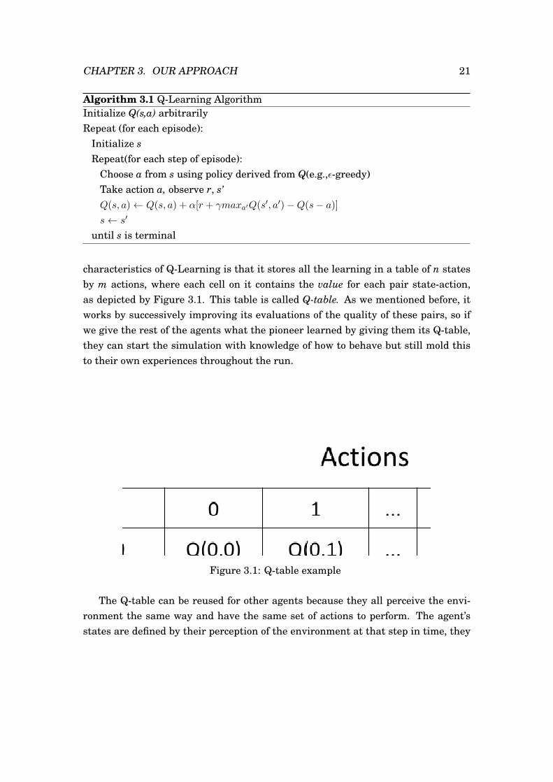
To properly function, our framework relies in two main modules that allows us tomake a separation between the agent and its surrounding environment. On the oneside, we have the Crowd Controller Module. This module is focused on all the du-ties that belong to the crowd simulation and feeding the information to the agents.On the other side we have the Reinforcement Learning Module, this one involves
CHAPTER 3. OUR APPROACH 23
everything that comes with the learning of the tasks at hand. The interaction be-tween these two is what allows us to simulate intelligent autonomous agents. Therelationship between the crowd controller and the reinforcement learning moduleis from 1 to n as depicted by Figure 3.2, where n is the amount of characters thatcompose the crowd. For a better understanding of these modules, we now proceedto explain them in a more detailed way.
Figure 3.2: Modules relationship
3.1 Crowd Controller Module
The crowd controller module is the main module in our project. It handles boththe rendering and setup of the simulation among other responsibilities, such ascontrolling the agents and giving them the pertinent information of their surround-ings. The controller module handles the simulation as depicted by Algorithm 3.3.Dividing the simulation by a prefixed amount of time intervals, the controller ateach time step will control every agent on the environment. Until the time intervalthat defines an episode is done, the controller will check the status of the agent,checking whether it has arrived to its goal point or not. In case it has not, it willprovide the information that affects that agent and then move it according to thefeedback it gets as a result.
This feedback comes from the interaction with the RL module that each agenthas assigned. The RL module decides the agent’s movements but the crowd con-troller actually moves the agent. Since this controller is the one in charge of all the
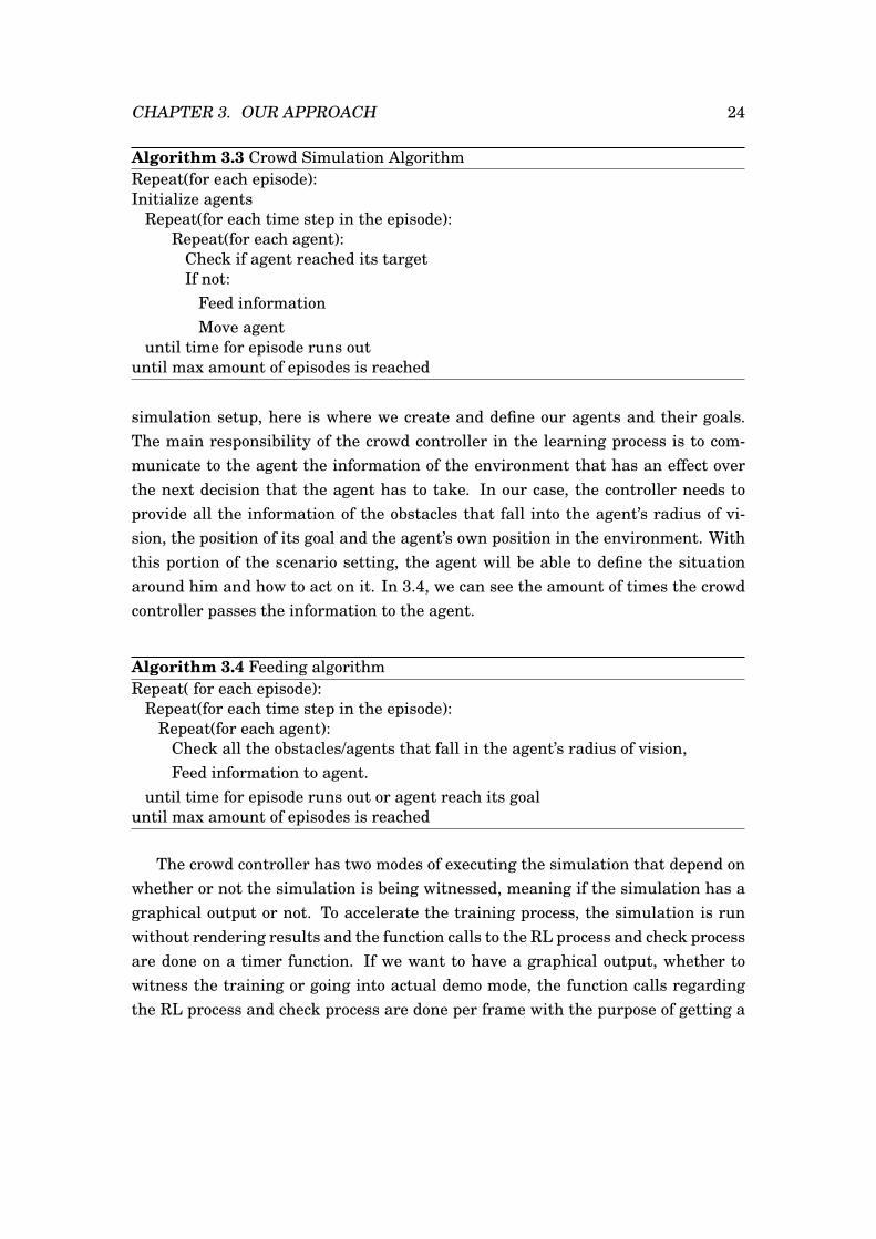
CHAPTER 3. OUR APPROACH 24
Algorithm 3.3 Crowd Simulation AlgorithmRepeat(for each episode):Initialize agents
Repeat(for each time step in the episode):Repeat(for each agent):
Check if agent reached its targetIf not:
Feed informationMove agent
until time for episode runs outuntil max amount of episodes is reached
simulation setup, here is where we create and define our agents and their goals.The main responsibility of the crowd controller in the learning process is to com-municate to the agent the information of the environment that has an effect overthe next decision that the agent has to take. In our case, the controller needs toprovide all the information of the obstacles that fall into the agent’s radius of vi-sion, the position of its goal and the agent’s own position in the environment. Withthis portion of the scenario setting, the agent will be able to define the situationaround him and how to act on it. In 3.4, we can see the amount of times the crowdcontroller passes the information to the agent.
Algorithm 3.4 Feeding algorithmRepeat( for each episode):
Repeat(for each time step in the episode):Repeat(for each agent):
Check all the obstacles/agents that fall in the agent’s radius of vision,Feed information to agent.
until time for episode runs out or agent reach its goaluntil max amount of episodes is reached
The crowd controller has two modes of executing the simulation that depend onwhether or not the simulation is being witnessed, meaning if the simulation has agraphical output or not. To accelerate the training process, the simulation is runwithout rendering results and the function calls to the RL process and check processare done on a timer function. If we want to have a graphical output, whether towitness the training or going into actual demo mode, the function calls regardingthe RL process and check process are done per frame with the purpose of getting a
CHAPTER 3. OUR APPROACH 25
graphical synchronized response.
3.2 Reinforcement Learning Module
The Reinforcement Learning module is the one we are really focused on this project.It is the core of the individual behavior of the agents. By using a reinforcementlearning library, we can create a learning machine for each agent so each one is aindividual with their our “brain”. The RL Module receives the information providedby the controller module and process it into states, the machine provides the agentwith an action to take following the ε-greedy policy, resulting in a movement thatis then evaluated by the RL Module, then fed to the machine that will process it toimprove the Q-table, from where it provides the “best” actions to take at each query.
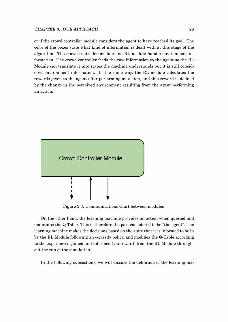
Even though we are making a separation between the RL Module responsibili-ties and the learning machine, the two of them are what really define the reinforce-ment learning module as a whole. This separation is described to show what arethe elements of the RL framework that we can actually modify so we can establishan agent/environment division of the elements. In Figure 3.3, we can see how thecommunication flows from a module to another. The dashed line represents the ini-tialization. The crowd controller module creates an agent, and for the first time, as-signs it its goal, current position and information pertinent to the escenario setting.The agent then proceeds to inform the RL Module to initialize its own RL Machineand to process the information given by the Crowd Controller Module. The RL Mod-ule informs the RL Machine the state the agent is in and asks for an action so theagent can perform according to this. The RL Machine now starts a cycle where itgives the RL Module an action for the agent to perform. The RL Module translatesthis action into a direction vector so the agent can be moved, and the agent informsthe crowd controller module where it has to go now. The crowd controller modulecalculates the pertinent information for that agent and at that moment and passesit along. The RL Module receives the information from the agent and process it intothe state resulting from performing the previous action and calculates the producedreward. The RL module communicates to the RL Machine the new state and thereward yielded so the machine responds to it with an action and now we are backat the starting point of the cycle.
This cycle will stop when the maximum amount of allowed decisions is reached
CHAPTER 3. OUR APPROACH 26
or if the crowd controller module considers the agent to have reached its goal. Thecolor of the boxes state what kind of information is dealt with at this stage of thealgorithm. The crowd controller module and RL module handle environment in-formation. The crowd controller feeds the raw information to the agent so the RLModule can translate it into states the machine understands but it is still consid-ered environment information. In the same way, the RL module calculates therewards given to the agent after performing an action, and this reward is definedby the change in the perceived environment resulting from the agent performingan action.
Figure 3.3: Communications chart between modules
On the other hand, the learning machine provides an action when queried andmaintains the Q-Table. This is therefore the part considered to be “the agent”. Thelearning machine makes the decisions based on the state that it is informed to be inby the RL Module following an ε-greedy policy, and modifies the Q-Table accordingto the experiences gained and informed (via reward) from the RL Module through-out the run of the simulation.
In the following subsections, we will discuss the definition of the learning ma-
CHAPTER 3. OUR APPROACH 27
chine and the main elements of our reinforcement learning problem.
3.2.1 Reinforcement Learning Library
As the core for our reinforcement learning module we used BaReL, a reinforcementlearning library developed by Jason Kastanis in 2008. BaReL offers reinforcementlearning algorithms for direct application in a basic way. We are able to create anRL application by using a minimum amount of functions. The main reason as towhy we used this library, besides its simplicity, is because it allows to both save andreuse the Q-table of the agent. We are able to save the Q-table to a .txt file at anytime, allowing us to create a record of learning every amount of episodes, and thenthis file can be loaded to the learning machine again to continue the learning, or inour case, to spread it to the other agents.
We made use of 8 of its functions to create our RL application, 3 of which areworth mentioning to help understanding the workflow of the RL process that in-volve the creation of the learning machine and the action queries.
Machine Creation
The machine creation is the first thing that has to be done after creating an agent.The machine will not only store the Q-table but it will also provide the actions whenqueried, and improve the knowledge acquired by the several experiences that re-ceives. As it was mentioned previously, the machine can be thought of as the brainof our agent and it has to be created and initialized before expecting the agent to doanything else.
To create and initialize the machine, BaReL offers among several options thefollowing:
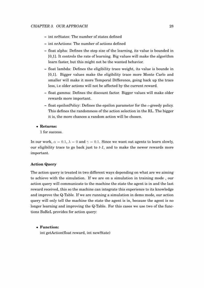
• Function:int createRLMachine(int nrStates, int nrActions, float alpha, float lambda,gamma, float epsilonPolicy)
• Parameters:
CHAPTER 3. OUR APPROACH 28
– int nrStates: The number of states defined
– int nrActions: The number of actions defined
– float alpha: Defines the step size of the learning, its value is bounded in[0,1]. It controls the rate of learning. Big values will make the algorithmlearn faster, but this might not be the wanted behavior.
– float lambda: Defines the eligibility trace weight, its value is bounde in[0,1]. Bigger values make the eligibility trace more Monte Carlo andsmaller will make it more Temporal Difference, going back up the traceless, i.e older actions will not be affected by the current reward.
– float gamma: Defines the discount factor. Bigger values will make olderrewards more important.
– float epsilonPolicy: Defines the epsilon parameter for the ε-greedy policy.This defines the randomness of the action selection in the RL. The biggerit is, the more chances a random action will be chosen.
• Returns:1 for success.
In our work, α = 0.1, λ = 0 and γ = 0.1. Since we want out agents to learn slowly,our eligibility trace to go back just to t-1, and to make the newer rewards moreimportant.
Action Query
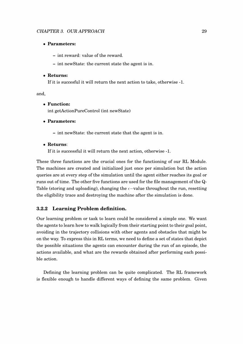
The action query is treated in two different ways depending on what are we aimingto achieve with the simulation. If we are on a simulation in training mode , ouraction query will communicate to the machine the state the agent is in and the lastreward received, this so the machine can integrate this experience to its knowledgeand improve the Q-Table. If we are running a simulation in demo mode, our actionquery will only tell the machine the state the agent is in, because the agent is nolonger learning and improving the Q-Table. For this cases we use two of the func-tions BaReL provides for action query:
• Function:int getAction(float reward, int newState)
CHAPTER 3. OUR APPROACH 29
• Parameters:
– int reward: value of the reward.
– int newState: the current state the agent is in.
• Returns:If it is succesful it will return the next action to take, otherwise -1.
and,
• Function:int getActionPureControl (int newState)
• Parameters:
– int newState: the current state that the agent is in.
• Returns:If it is successful it will return the next action, otherwise -1.
These three functions are the crucial ones for the functioning of our RL Module.The machines are created and initialized just once per simulation but the actionqueries are at every step of the simulation until the agent either reaches its goal orruns out of time. The other five functions are used for the file management of the Q-Table (storing and uploading), changing the ε−value throughout the run, resettingthe eligibility trace and destroying the machine after the simulation is done.
3.2.2 Learning Problem definition.
Our learning problem or task to learn could be considered a simple one. We wantthe agents to learn how to walk logically from their starting point to their goal point,avoiding in the trajectory collisions with other agents and obstacles that might beon the way. To express this in RL terms, we need to define a set of states that depictthe possible situations the agents can encounter during the run of an episode, theactions available, and what are the rewards obtained after performing each possi-ble action.
Defining the learning problem can be quite complicated. The RL frameworkis flexible enough to handle different ways of defining the same problem. Given
CHAPTER 3. OUR APPROACH 30
that we are aiming to use the same Q-table for different scenarios and on differentagents, our goal is to be as general as possible when defining our RL elements.Keeping this in mind, we now proceed to introduce the solution adopted for eachelement of our RL Problem.
3.2.2.1 State definition
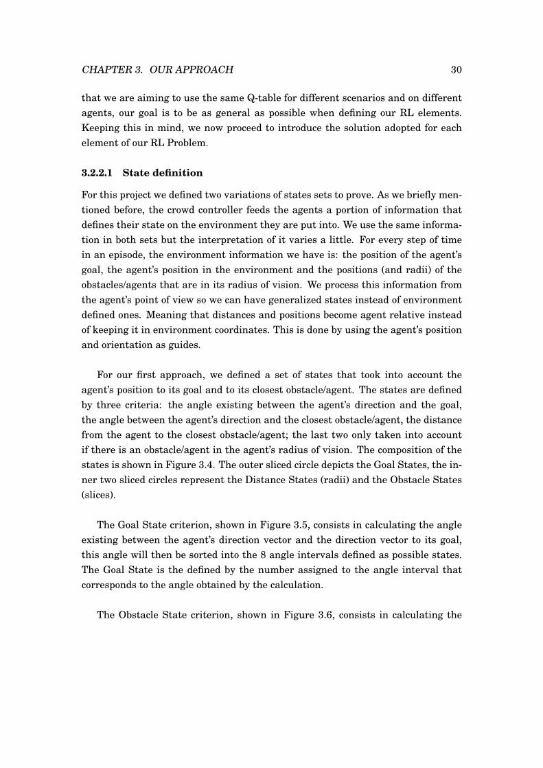
For this project we defined two variations of states sets to prove. As we briefly men-tioned before, the crowd controller feeds the agents a portion of information thatdefines their state on the environment they are put into. We use the same informa-tion in both sets but the interpretation of it varies a little. For every step of timein an episode, the environment information we have is: the position of the agent’sgoal, the agent’s position in the environment and the positions (and radii) of theobstacles/agents that are in its radius of vision. We process this information fromthe agent’s point of view so we can have generalized states instead of environmentdefined ones. Meaning that distances and positions become agent relative insteadof keeping it in environment coordinates. This is done by using the agent’s positionand orientation as guides.
For our first approach, we defined a set of states that took into account theagent’s position to its goal and to its closest obstacle/agent. The states are definedby three criteria: the angle existing between the agent’s direction and the goal,the angle between the agent’s direction and the closest obstacle/agent, the distancefrom the agent to the closest obstacle/agent; the last two only taken into accountif there is an obstacle/agent in the agent’s radius of vision. The composition of thestates is shown in Figure 3.4. The outer sliced circle depicts the Goal States, the in-ner two sliced circles represent the Distance States (radii) and the Obstacle States(slices).
The Goal State criterion, shown in Figure 3.5, consists in calculating the angleexisting between the agent’s direction vector and the direction vector to its goal,this angle will then be sorted into the 8 angle intervals defined as possible states.The Goal State is the defined by the number assigned to the angle interval thatcorresponds to the angle obtained by the calculation.
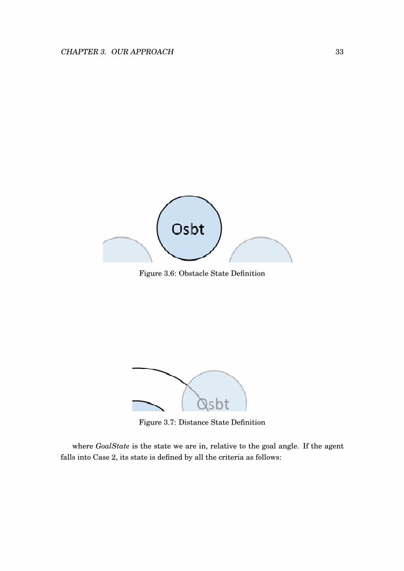
The Obstacle State criterion, shown in Figure 3.6, consists in calculating the

CHAPTER 3. OUR APPROACH 31
Figure 3.4: Composition of States
angle existing between the agent’s direction vector and the direction vector fromit to the nearest obstacle, this angle will then be sorted into the 8 angle intervalsdefined as possible states. As we can see in the figure, the division of the angles intointervals is not even as in the Goal State criterion. This is because we consideredmore important to discretize the states regarding what is happening in front of theagent and not at the back of it. We could have done as many partitions in the backas in the front of the agent, but this would have lead to a much larger memory spaceto store the Q-Table.
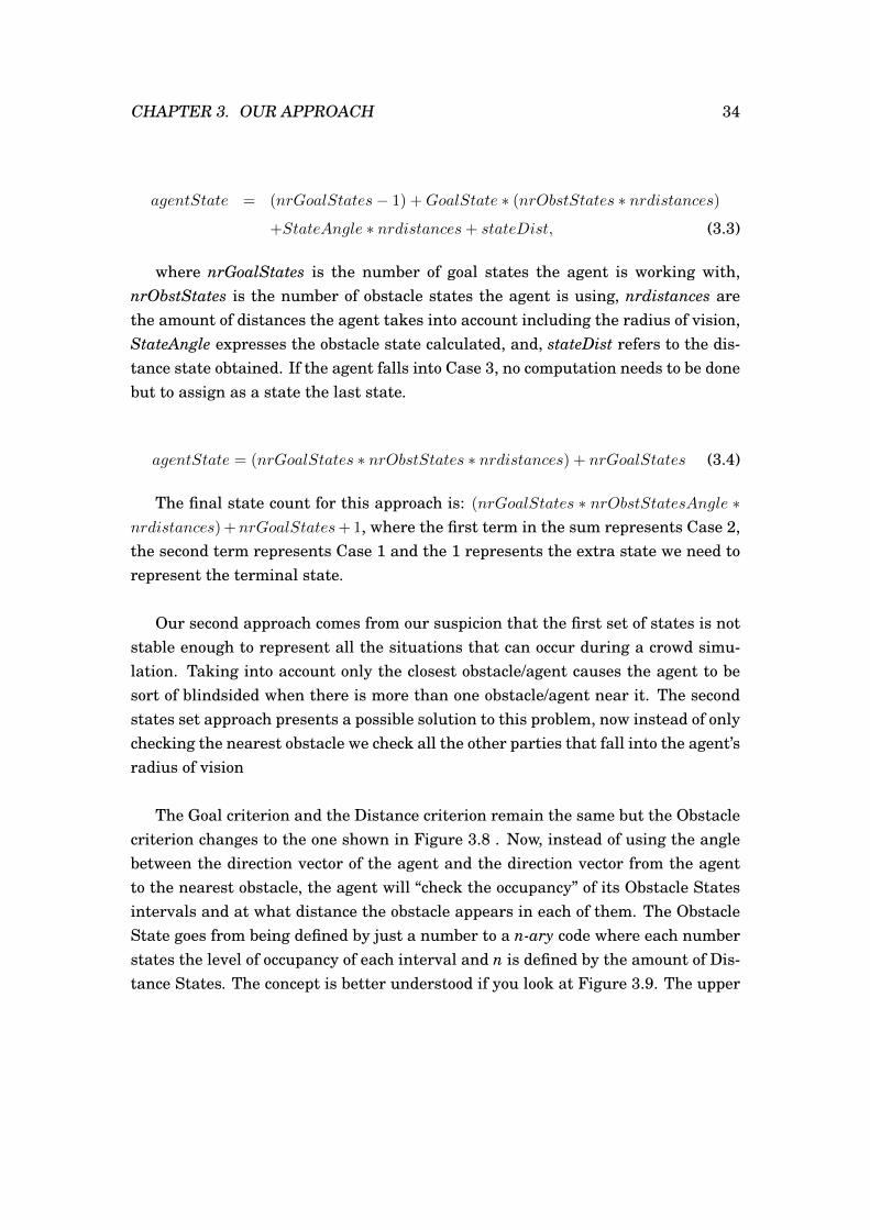
The Distance State criterion, shown in Figure 3.7 , consists in calculating thedistance existing between the agent and its nearest obstacle. This is done by mea-suring the distance between the agent and the center of the obstacle and then sub-tracting the radius of it. This result is then placed in the corresponding distanceinterval that will define the distance state. A distance state of 0 means that there isno obstacle in the radius of vision, a distance state of 1 establishes the presence ofthe obstacle in the nearest radius to the agent, and from this, the numbering growsuntil it reaches the radius of vision.
CHAPTER 3. OUR APPROACH 32
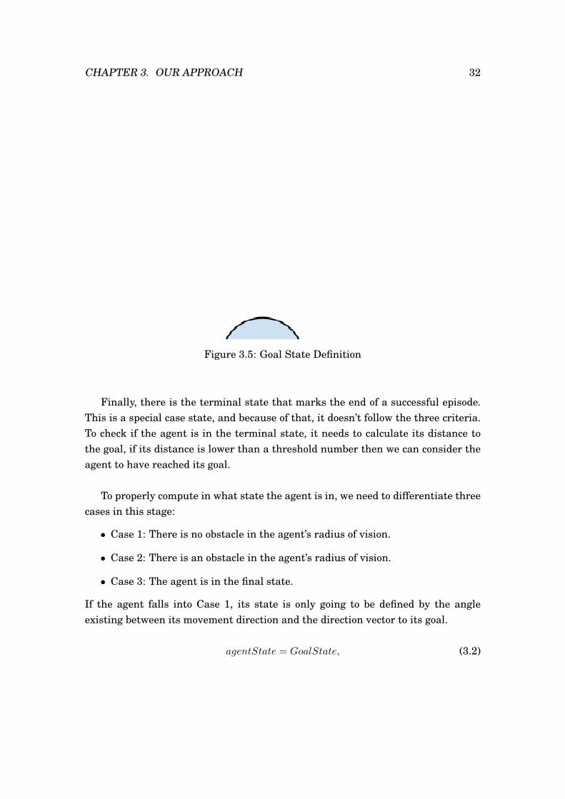
Figure 3.5: Goal State Definition
Finally, there is the terminal state that marks the end of a successful episode.This is a special case state, and because of that, it doesn’t follow the three criteria.To check if the agent is in the terminal state, it needs to calculate its distance tothe goal, if its distance is lower than a threshold number then we can consider theagent to have reached its goal.
To properly compute in what state the agent is in, we need to differentiate threecases in this stage:
• Case 1: There is no obstacle in the agent’s radius of vision.
• Case 2: There is an obstacle in the agent’s radius of vision.
• Case 3: The agent is in the final state.
If the agent falls into Case 1, its state is only going to be defined by the angleexisting between its movement direction and the direction vector to its goal.
agentState = GoalState, (3.2)
CHAPTER 3. OUR APPROACH 33
Figure 3.6: Obstacle State Definition
Figure 3.7: Distance State Definition
where GoalState is the state we are in, relative to the goal angle. If the agentfalls into Case 2, its state is defined by all the criteria as follows:
CHAPTER 3. OUR APPROACH 34
agentState = (nrGoalStates− 1) +GoalState ∗ (nrObstStates ∗ nrdistances)
+StateAngle ∗ nrdistances+ stateDist, (3.3)
where nrGoalStates is the number of goal states the agent is working with,nrObstStates is the number of obstacle states the agent is using, nrdistances arethe amount of distances the agent takes into account including the radius of vision,StateAngle expresses the obstacle state calculated, and, stateDist refers to the dis-tance state obtained. If the agent falls into Case 3, no computation needs to be donebut to assign as a state the last state.
agentState = (nrGoalStates ∗ nrObstStates ∗ nrdistances) + nrGoalStates (3.4)
The final state count for this approach is: (nrGoalStates ∗ nrObstStatesAngle ∗nrdistances)+nrGoalStates+1, where the first term in the sum represents Case 2,the second term represents Case 1 and the 1 represents the extra state we need torepresent the terminal state.
Our second approach comes from our suspicion that the first set of states is notstable enough to represent all the situations that can occur during a crowd simu-lation. Taking into account only the closest obstacle/agent causes the agent to besort of blindsided when there is more than one obstacle/agent near it. The secondstates set approach presents a possible solution to this problem, now instead of onlychecking the nearest obstacle we check all the other parties that fall into the agent’sradius of vision
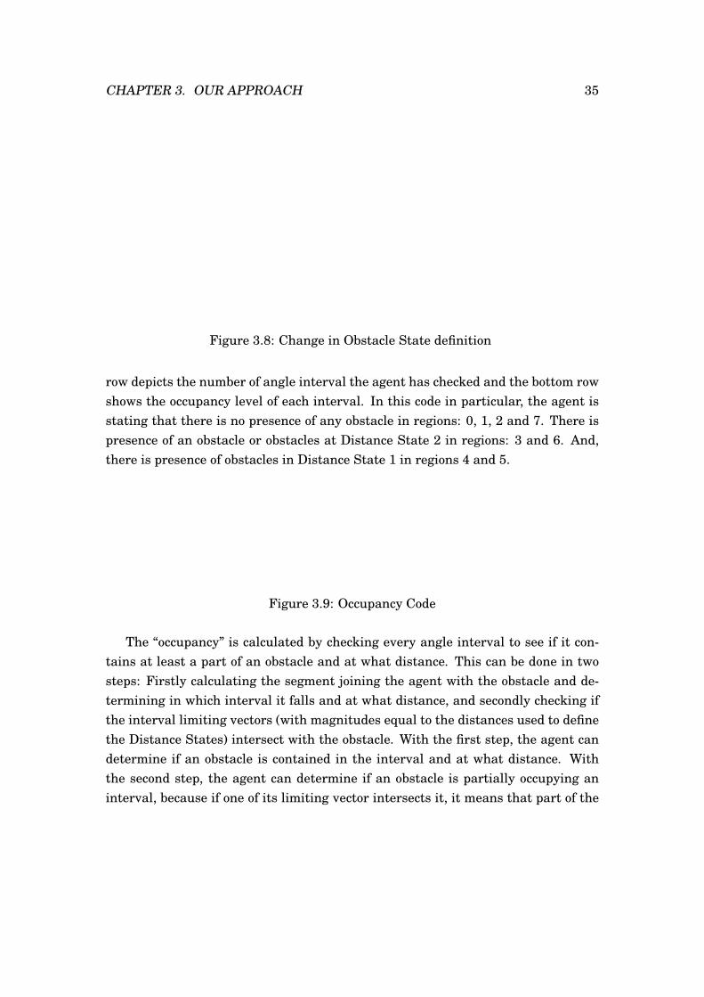
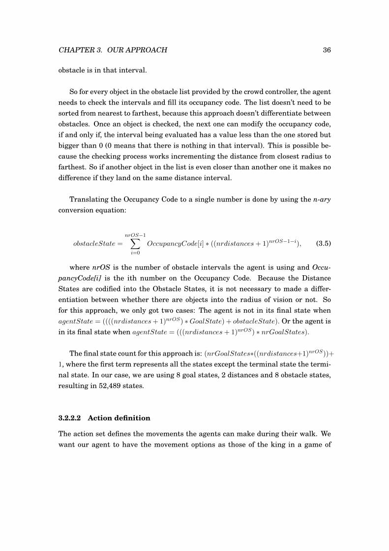
The Goal criterion and the Distance criterion remain the same but the Obstaclecriterion changes to the one shown in Figure 3.8 . Now, instead of using the anglebetween the direction vector of the agent and the direction vector from the agentto the nearest obstacle, the agent will “check the occupancy” of its Obstacle Statesintervals and at what distance the obstacle appears in each of them. The ObstacleState goes from being defined by just a number to a n-ary code where each numberstates the level of occupancy of each interval and n is defined by the amount of Dis-tance States. The concept is better understood if you look at Figure 3.9. The upper
CHAPTER 3. OUR APPROACH 35
Figure 3.8: Change in Obstacle State definition
row depicts the number of angle interval the agent has checked and the bottom rowshows the occupancy level of each interval. In this code in particular, the agent isstating that there is no presence of any obstacle in regions: 0, 1, 2 and 7. There ispresence of an obstacle or obstacles at Distance State 2 in regions: 3 and 6. And,there is presence of obstacles in Distance State 1 in regions 4 and 5.
Figure 3.9: Occupancy Code
The “occupancy” is calculated by checking every angle interval to see if it con-tains at least a part of an obstacle and at what distance. This can be done in twosteps: Firstly calculating the segment joining the agent with the obstacle and de-termining in which interval it falls and at what distance, and secondly checking ifthe interval limiting vectors (with magnitudes equal to the distances used to definethe Distance States) intersect with the obstacle. With the first step, the agent candetermine if an obstacle is contained in the interval and at what distance. Withthe second step, the agent can determine if an obstacle is partially occupying aninterval, because if one of its limiting vector intersects it, it means that part of the
CHAPTER 3. OUR APPROACH 36
obstacle is in that interval.
So for every object in the obstacle list provided by the crowd controller, the agentneeds to check the intervals and fill its occupancy code. The list doesn’t need to besorted from nearest to farthest, because this approach doesn’t differentiate betweenobstacles. Once an object is checked, the next one can modify the occupancy code,if and only if, the interval being evaluated has a value less than the one stored butbigger than 0 (0 means that there is nothing in that interval). This is possible be-cause the checking process works incrementing the distance from closest radius tofarthest. So if another object in the list is even closer than another one it makes nodifference if they land on the same distance interval.
Translating the Occupancy Code to a single number is done by using the n-aryconversion equation:
obstacleState =
nrOS−1∑i=0
OccupancyCode[i] ∗ ((nrdistances+ 1)nrOS−1−i), (3.5)
where nrOS is the number of obstacle intervals the agent is using and Occu-pancyCode[i] is the ith number on the Occupancy Code. Because the DistanceStates are codified into the Obstacle States, it is not necessary to made a differ-entiation between whether there are objects into the radius of vision or not. Sofor this approach, we only got two cases: The agent is not in its final state whenagentState = ((((nrdistances+ 1)nrOS) ∗GoalState) + obstacleState). Or the agent isin its final state when agentState = (((nrdistances+ 1)nrOS) ∗ nrGoalStates).
The final state count for this approach is: (nrGoalStates∗((nrdistances+1)nrOS))+
1, where the first term represents all the states except the terminal state the termi-nal state. In our case, we are using 8 goal states, 2 distances and 8 obstacle states,resulting in 52,489 states.
3.2.2.2 Action definition
The action set defines the movements the agents can make during their walk. Wewant our agent to have the movement options as those of the king in a game of

CHAPTER 3. OUR APPROACH 37
chess. Meaning that our agents can move in 8 different directions as depicted inFigure 3.10a. Similar as with the states, the actions are defined using the agent’sorientation as pivot or guide. For that reason, the actions are defined relatively tothis direction vector, being the set of actions a result of rotations in the Y axis ofthe orientation vector. For consistency, each action is always defined by the sameangle (e.g. action 1 will always mean no rotation at all, action 2 will always meanrotation of 180 degrees, etc) as can be seen in Figure 3.10b.
(a) (b)
Figure 3.10: Description of movements: (a) King’s movements (b) Action definitionby rotation of orientation vector
So every time an action is chosen, translating this action to a movement is per-formed by taking the orientation vector at that moment and applying a rotation tothis vector. The resulting vector is the agent’s new direction hence will be takenas a reference for the next action chosen. Allowing for a set of actions to remainrelative to the agent’s orientation helps to create a more human like path.
3.2.2.3 Reward function
The reward function defines what we want the agent to learn. Through this incen-tive, the agent will reach its goal as long as we formulate it properly. There aretwo things that the agents need to learn in order to reach its goal successfully: (1)
CHAPTER 3. OUR APPROACH 38
Crashing into or going through objects needs to be severely punished while movingtowards its goal and walking coherently has to be rewarded positively.
The reward function can vary depending on the set of states we are using,what we consider that “walking coherently” means and whether the agent reachedits goal or not. The general formula of the reward is very simple: r(st, at) =
rewardGoal+rewardObstacle. With the special case being that the agent has reachedits goal, in which case we just assign a reward of 100.
Consider rewardGoal the reward we assign for walking coherently towards itsgoal. For us, this derived in two options: either we rewarded the agent the dis-tance it gained by choosing said action in said state or we formulated the rewardby assigning it the cosine of the angle resulting from its chosen direction and thedirection vector to the goal. One is less straightforward than the other but both tryto establish the same principle, walking straight to the goal is the best option. Inthe case of distance gained per step, the reward comes defined by:
rewardGoal = |−−→pd2g| − |
−−→cd2g|, (3.6)
where−−→pd2g is the previous direction vector existing between the agent and the goal,
and−−→cd2g is the current direction vector existing from the agent to the goal. This re-
sults in positive rewards when the agent is getting nearer to the goal and negativerewards if the breach between them grows. In Figure 3.11, we show graphicallywhat this difference means. In 3.11a, we can clearly see that
−−→pd2g represents the
direction vector to the goal that existed in t− 1, hence its faded,−−→cd2g is represented
in a solid black color meaning that it is the direction vector to the goal in the currenttime t. This reward function works because of the two simple cases that occur. Incase a , as showed in 3.11b, the magnitude of
−−→pd2g is smaller than the magnitude of
−−→cd2g, meaning that the agent instead of approaching the goal is going in a directionthat is making the distance longer and the difference between these will give it anegative reward, while in case b, the magnitude of
−−→cd2g is smaller than the mag-
nitude of−−→pd2g, which means the agent is getting closer and the difference between
these will give it a positive reward.
Implicitly, we are teaching the agent that the best way to walk towards the goalis in a straight line from its birthing point to its goal point, because the reward de-

CHAPTER 3. OUR APPROACH 39
fines as distance gain gets greater at every step if it does not deviate from it. Sidesteps, angular steps and backward steps will not yield such a high reward.
(a) (b)
Figure 3.11: Distance Gain: (a) Direction Vector to the goal in t-1 and t, (b) Casesof distance gain.
Our second option for a rewardGoal takes another approach to inducing theagent to learn to walk in a straight line to its goal. In this case, instead of takinginto account the distance gained at every step, we want to consider how much alikeis its direction of movement to the direction vector pointing towards the goal. Thisreward function can be defined as:
rewardGoal = cos(angle(−−→cd2g,
−−−−−−−−→currentDir))3, (3.7)
where−−→cd2g remains to be the current direction vector from the agent to its goal
and−−−−−−−−→currentDir is the current direction vector of the agent. Using the cosine of the
angle between these vectors results in a reward that is better when the agent’s di-rection movement tends to the direction vector to the goal, and diminishes as thedifference between them increases. For a better understanding of the concept, wecan see this in Figure 3.12. We decided to use the cube value of the cosine to makethe function decrease faster the farther is the direction vector of the agent to coin-cide with
−−→cd2g as shown in Figure 3.12b. This favors more directions that are closer
to the desired one. In this manner, we are directly communicating to the agent thatkeeping the direction of movement as close as possible to the direction vector point-
CHAPTER 3. OUR APPROACH 40
ing towards the goal, is its best option reward wise, and this translates to walkingin a straight line.
(a)
(b)
Figure 3.12: Reward by Cosine: (a) Direction Vector to the goal and Agent’s direc-tion vector, (b) Some of the reward values for certain angles
Now for the rewardObstacle definition we have to differentiate between the twostate sets we previously defined. In the first approach it is straight forward, if thereis an obstacle in the nearest radius of distance, this is considered a collision, and forthis reason it is severely punished by setting the rewardObstacle to -80. If there isno obstacle, the reward will be set to 0 because it does not affect the agent’s decision.And finally, if the obstacle is not crashing but it is perceived by the agent, dependingon the radius of distance it is detected we calculate the reward as follows:
rewardObstacle = −80/102i, (3.8)
where i is the ith closest distance to the agent’s nearest radius (e.g: if i = 1 itmeans that it is the first distance after the nearest one to the agent, so the penaltywill be -0.8). This penalty is used as a warning that the decision that it made mighttake him in the wrong direction and will help with stearing the agent before itcrashes with the obstacle. Notice that the penalties are bigger than the positiverewards and this is because we need the agent to learn that even though walking
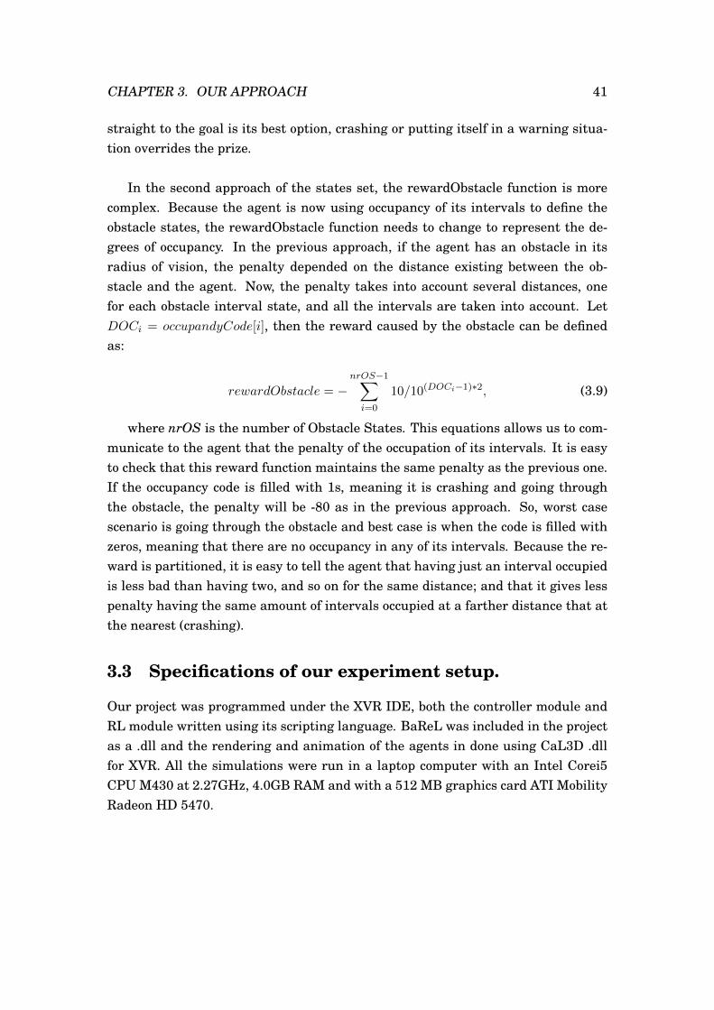
CHAPTER 3. OUR APPROACH 41
straight to the goal is its best option, crashing or putting itself in a warning situa-tion overrides the prize.
In the second approach of the states set, the rewardObstacle function is morecomplex. Because the agent is now using occupancy of its intervals to define theobstacle states, the rewardObstacle function needs to change to represent the de-grees of occupancy. In the previous approach, if the agent has an obstacle in itsradius of vision, the penalty depended on the distance existing between the ob-stacle and the agent. Now, the penalty takes into account several distances, onefor each obstacle interval state, and all the intervals are taken into account. LetDOCi = occupandyCode[i], then the reward caused by the obstacle can be definedas:
rewardObstacle = −nrOS−1∑i=0
10/10(DOCi−1)∗2, (3.9)
where nrOS is the number of Obstacle States. This equations allows us to com-municate to the agent that the penalty of the occupation of its intervals. It is easyto check that this reward function maintains the same penalty as the previous one.If the occupancy code is filled with 1s, meaning it is crashing and going throughthe obstacle, the penalty will be -80 as in the previous approach. So, worst casescenario is going through the obstacle and best case is when the code is filled withzeros, meaning that there are no occupancy in any of its intervals. Because the re-ward is partitioned, it is easy to tell the agent that having just an interval occupiedis less bad than having two, and so on for the same distance; and that it gives lesspenalty having the same amount of intervals occupied at a farther distance that atthe nearest (crashing).
3.3 Specifications of our experiment setup.
Our project was programmed under the XVR IDE, both the controller module andRL module written using its scripting language. BaReL was included in the projectas a .dll and the rendering and animation of the agents in done using CaL3D .dllfor XVR. All the simulations were run in a laptop computer with an Intel Corei5CPU M430 at 2.27GHz, 4.0GB RAM and with a 512 MB graphics card ATI MobilityRadeon HD 5470.

Chapter 4
Results
In this chapter we will present the results of the tests we considered important toapply to the different elements of our RL method. First, we will evaluate the twoproposed reward functions in our first states set approach using just one agent.This will help us to decide which one of the proposed reward functions is betterfor our purpose. Then, we proceed to explain why there was a need for a secondapproach of states set and what were the weaknesses of our first approach. Lastly,we will present a set of images that depict the results of some of the simulations weran using our proposed method.
4.1 Evaluation of the reward function.
To evaluate the reward functions, we decided to do some tests using both functionspaired with our first states set approach. Both simulations were run twice each.Once for the training process, and another one for the demo simulation. Four mea-surements were taken each time for each reward function, the agent learning andusing its knowledge on the same environment setting depicted by Figure 4.1. Theagent starts each episode near the center of the scenario, with an obstacle betweenit and its goal. The agent moves in the direction provided by the RL Module witha velocity of 0.03 units/step, it works with two radii inside its radius of vision, thecloser one (red circle) at 0.5 units from its center and the second one (gray surround-ing area) at 1 unit from it.
As specified before, the agent will not know where the obstacle is at all times
42

CHAPTER 4. RESULTS 43
but it always knows where its goal is at. The detection of the obstacle starts whenat least a point of its perimeter comes into contact with the grey area, if it comesinto contact with the red area it is then considered a crash.
We thought of a set of measurements that could give us some useful informationto verify if the reward function being used is achieving our goals, that are the fol-lowing: the agent reaching its goal, the agent avoiding the obstacle and the agentwalking coherently during the episode. To evade the agent learning to walk in astatic setting, the goal’s position varies from episode to episode, allowing the agentto be exposed to different situations and have a richer Q-Table.
Figure 4.1: Reward Function Evaluation: Tests Setting
Each simulation is composed by 2000 episodes, and each episode lasts until theagent reaches its goal ,or it reaches 2000 decisions made. In the four simulationswe will measure the same four values, two per episode and two as overall evalua-tions of the simulation.
The episode evaluation consists of two measurements: the ratio of distancegained towards the goal per step, and the ratio of the real path followed against thedistance gained towards the goal. The first measurement is pretty much straightforward. This ratio defines the average distance gained for every step taken duringan episode. Our agent has a constant velocity throughout the simulation (0.03 unitsper step), this is multiplied to the direction vector obtained from the RL module andthe result is added to its current position, resulting in the agent’s movement. If we

CHAPTER 4. RESULTS 44
take the accumulated distance gained and divide it by the number of steps thatthe agent took during the episode, we can observe the average velocity the agenthad during the run of the episode. In subsection 3.2.2.3, we defined that walkingcoherently means going in a straight line towards its goal. For this reason, if wetake the ratio of distance gained per step and we compare it to the agent’s velocity.Depending on the similarity between this value and the real velocity we can deter-mine how good the decisions made during this episode were.
Likewise, we can study the relationship between the path followed and the dis-tance gained. Consider the path followed is the accumulation of all the distanceswalked byt the agent during the episode. In the best case scenario, dividing thepath followed by the distance gained should be as close as possible to 1. This meansthat the agent followed the most efficient path towards the goal. Since we are in asetting where there is an obstacle on the way to the goal, this ratio will not be equalto 1 but smaller values mean better results.
For the evaluation of the simulation we considered the rate of success and therate of collisions to be really important. To avoid absorbing states that can perpet-uate the simulation, our episodes are capped at 2000 decisions if the agent doesn’treach its goal. If that is the case, then the episode is counted as a failed episode.Ultimately, it could be considered that the agent’s primary objective is to reach itsgoal. Knowing the rate of success can help us weight the options.
Finally, the rate of collisions informs us about the percentage of episodes theagent where collisioned with the obstacle. The agent should avoid obstacles andnever go through them for the simulation to be realistic. As the agent gains experi-ence the number of collisions should decrease. A collision occurs when an obstacleor another agent enters the closest radius of the agent’s radius of vision.
4.1.1 Training Process
During the training process we obtained the following measurements of the perfor-mance of each reward function. These results are partial because, during training,the learning machine follows the ε-greey policy inserting randomness in the deci-sion making (action selection).
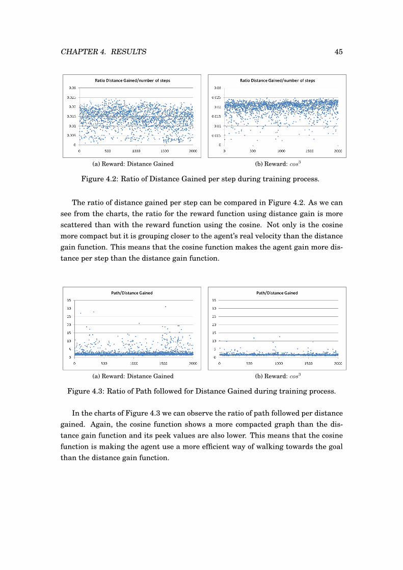
CHAPTER 4. RESULTS 45
(a) Reward: Distance Gained (b) Reward: cos3
Figure 4.2: Ratio of Distance Gained per step during training process.
The ratio of distance gained per step can be compared in Figure 4.2. As we cansee from the charts, the ratio for the reward function using distance gain is morescattered than with the reward function using the cosine. Not only is the cosinemore compact but it is grouping closer to the agent’s real velocity than the distancegain function. This means that the cosine function makes the agent gain more dis-tance per step than the distance gain function.
(a) Reward: Distance Gained (b) Reward: cos3
Figure 4.3: Ratio of Path followed for Distance Gained during training process.
In the charts of Figure 4.3 we can observe the ratio of path followed per distancegained. Again, the cosine function shows a more compacted graph than the dis-tance gain function and its peek values are also lower. This means that the cosinefunction is making the agent use a more efficient way of walking towards the goalthan the distance gain function.

CHAPTER 4. RESULTS 46
(a) Reward: Distance Gained (b) Reward: cos3
Figure 4.4: Rate of success during training process
The rate of success during training proves to be better for the cosine functionthan the distance gain function, as it is shown in Figure 4.4. The 0.40% failure inthe cosine chart means that only 8 out of the 2000 episodes did not finish positively.With the distance gain reward function the number goes up to 155 episodes out of2000.
(a) Reward: Distance Gained (b) Reward: cos3
Figure 4.5: Rate of collisions during training process
Now the collision rate in Figure 4.5 shows us a very interesting behavior. Thedistance gain reward function worked better at avoiding collisions than the cosinereward function. The percentages show that the agent can achieve almost totalavoidance by using the distance gain reward function, while the cosine reward func-tion presented a higher incidence of episodes with collisions.

CHAPTER 4. RESULTS 47
We can infer from these partial results, that there is a tendency of the distancegain reward function to induce the agent to follow longer paths, and approach thegoal slowly in order to avoid obstacles.
4.1.2 Demo Simulation
The next set of charts are a depiction of the results obtained from running the simu-lation in demo mode (choosing the actions without randomness), using the Q-Tablesresulting from the previous training processes. With this information, we can un-derstand what the agent learned in each training process and we can weight ouroptions regarding the reward function to use for our crowd simulation.
(a) Reward: Distance Gained (b) Reward: cos3
Figure 4.6: Ratio of Distance Gained per step during demo simulation.
In Figure 4.6, we can see a separation present in both charts. This could meanthat the amount of episodes used for the training process were insufficient and theagent still makes poor decisions when it comes to moving towards the goal. How-ever, the ratio seems to converge closer to the real velocity in the simulation madewith the cosine reward function than the simulation made with the distance gainreward function.
The ratios of path taken for distance gained in Figure 4.7 shows us how both re-ward functions are converging below 5, but the cosine reward function looks morecompact than the distance gain reward function. Still there are too many scatteredvalues to tell which option is best in this case.

CHAPTER 4. RESULTS 48
(a) Reward: Distance Gained (b) Reward: cos3
Figure 4.7: Ratio of Path followed for Distance Gained during demo simulation.
(a) Reward: Distance Gained (b) Reward: cos3
Figure 4.8: Rate of success during demo simulation.
The success rate presented in Figure 4.8, is inconclusive too. The distance gainreward function yielded a 26.20% of episodes ended without the agent achieving itsgoal, while the cosine reward function was slightly better with a 20.90%. Compar-ing these results to our partial results during training makes clear that both train-ing processes needed more episodes to improve the Q-Tables, or that the amount ofdecisions made for episode should be bigger.
The collision rate charts in Figure 4.9, shows us that the distance gain rewardfunction was effective in teaching the agent to avoid collisions. But when the agentgot its rewards from the cosine function, avoiding obstacles does not seem to be astrict priority.
After analizing these measurement, we now can conclude that the distance gain
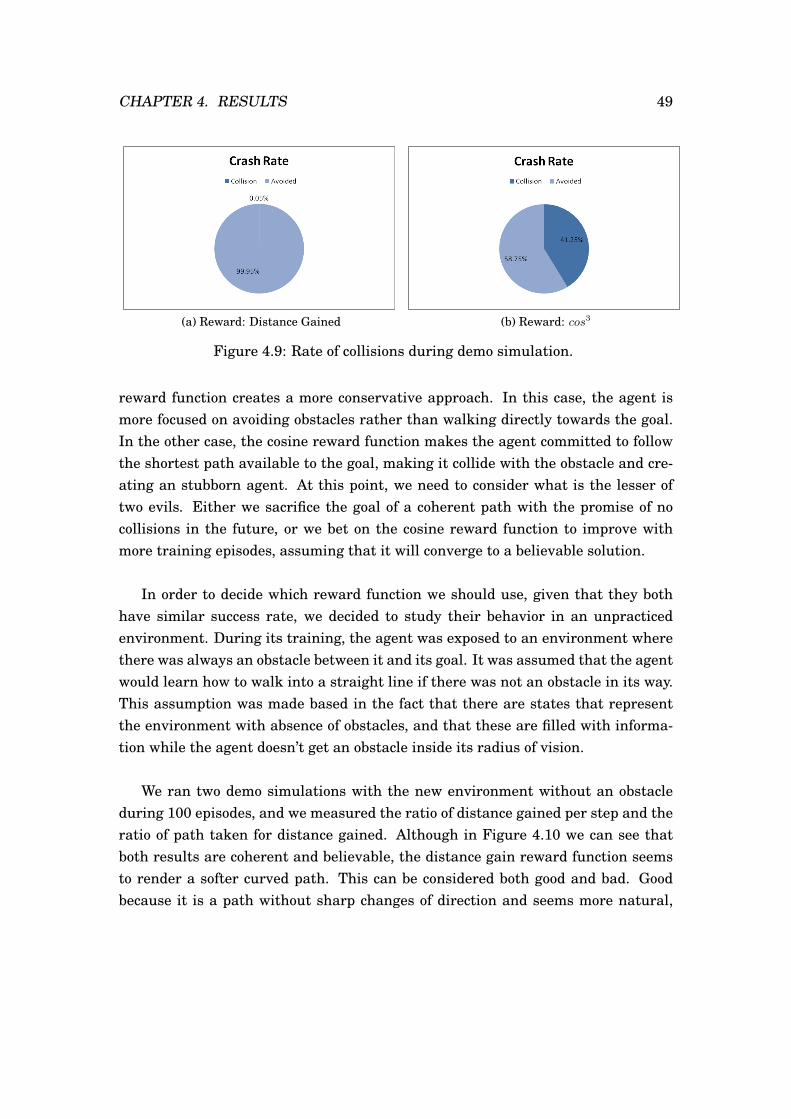
CHAPTER 4. RESULTS 49
(a) Reward: Distance Gained (b) Reward: cos3
Figure 4.9: Rate of collisions during demo simulation.
reward function creates a more conservative approach. In this case, the agent ismore focused on avoiding obstacles rather than walking directly towards the goal.In the other case, the cosine reward function makes the agent committed to followthe shortest path available to the goal, making it collide with the obstacle and cre-ating an stubborn agent. At this point, we need to consider what is the lesser oftwo evils. Either we sacrifice the goal of a coherent path with the promise of nocollisions in the future, or we bet on the cosine reward function to improve withmore training episodes, assuming that it will converge to a believable solution.
In order to decide which reward function we should use, given that they bothhave similar success rate, we decided to study their behavior in an unpracticedenvironment. During its training, the agent was exposed to an environment wherethere was always an obstacle between it and its goal. It was assumed that the agentwould learn how to walk into a straight line if there was not an obstacle in its way.This assumption was made based in the fact that there are states that representthe environment with absence of obstacles, and that these are filled with informa-tion while the agent doesn’t get an obstacle inside its radius of vision.
We ran two demo simulations with the new environment without an obstacleduring 100 episodes, and we measured the ratio of distance gained per step and theratio of path taken for distance gained. Although in Figure 4.10 we can see thatboth results are coherent and believable, the distance gain reward function seemsto render a softer curved path. This can be considered both good and bad. Goodbecause it is a path without sharp changes of direction and seems more natural,

CHAPTER 4. RESULTS 50
(a) Reward: Distance Gained (b) Reward: cos3
Figure 4.10: Results of simulation on an environment without obstacle.
but bad because there is no reason for the agent to deviate from the straight linegiven that there is no obstacle in the way.
(a) Reward: Distance Gained (b) Reward: cos3
Figure 4.11: Ratio of Distance Gained per step during simulation without an obsta-cle.
The visual results induce us to think that with the distance gain reward func-tion, the agent isn’t learning to walk in a straight line to the goal, but we cannotmake decisions only basing this assumption in the visual results. In relation to theratio of distance gained per step, as shown in Figure 4.11, we can witness that thevelocity during the simulation with the distance gain reward function is lower thanthe velocity reached with the cosine reward function, stating that the agent mightbe doing a better looking path with the distance gain reward function, but this isachieved only by using more steps and gaining less distance with each of them. Thecosine reward function shows a more consistent velocity between episodes, even
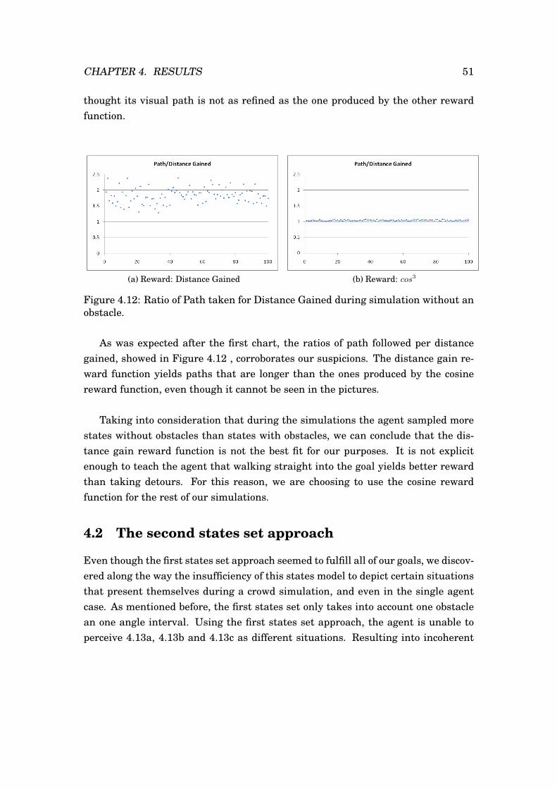
CHAPTER 4. RESULTS 51
thought its visual path is not as refined as the one produced by the other rewardfunction.
(a) Reward: Distance Gained (b) Reward: cos3
Figure 4.12: Ratio of Path taken for Distance Gained during simulation without anobstacle.
As was expected after the first chart, the ratios of path followed per distancegained, showed in Figure 4.12 , corroborates our suspicions. The distance gain re-ward function yields paths that are longer than the ones produced by the cosinereward function, even though it cannot be seen in the pictures.
Taking into consideration that during the simulations the agent sampled morestates without obstacles than states with obstacles, we can conclude that the dis-tance gain reward function is not the best fit for our purposes. It is not explicitenough to teach the agent that walking straight into the goal yields better rewardthan taking detours. For this reason, we are choosing to use the cosine rewardfunction for the rest of our simulations.
4.2 The second states set approach
Even though the first states set approach seemed to fulfill all of our goals, we discov-ered along the way the insufficiency of this states model to depict certain situationsthat present themselves during a crowd simulation, and even in the single agentcase. As mentioned before, the first states set only takes into account one obstaclean one angle interval. Using the first states set approach, the agent is unable toperceive 4.13a, 4.13b and 4.13c as different situations. Resulting into incoherent

CHAPTER 4. RESULTS 52
decisions when these situations occur (the agent could end up inside an obstacle orwalking farther from it than needed)
(a) (b) (c)
Figure 4.13: Same state definition for different situations
Another similar issue of this states set is the inability to deal with tricky situa-tions. Imagine an environment where two obstacles are too close to each other forthe agent to walk between them. We would expect the agent to avoid taking thatpath because the negative reward yielded for going through an obstacle is consider-ably big. As we can see in Figure 4.14, if the agent is oblivious to the existence ofthe other obstacle (4.14a) , it will behave as expected. Confusion comes from havingtwo obstacles inside its radius of vision (4.14b, 4.14c). Since it can only choose oneobstacle and assign it to just one of its angle intervals, the agent does not have graspof the complete situation, ending up taking decisions under wrongful assumptionsresulting in artifacts.
(a) (b) (c)
Figure 4.14: Twins Test for first state set approach
These poor decisions could be blamed on an incomplete training process, butthere is no way for the agent to learn to avoid these situations if the experiences
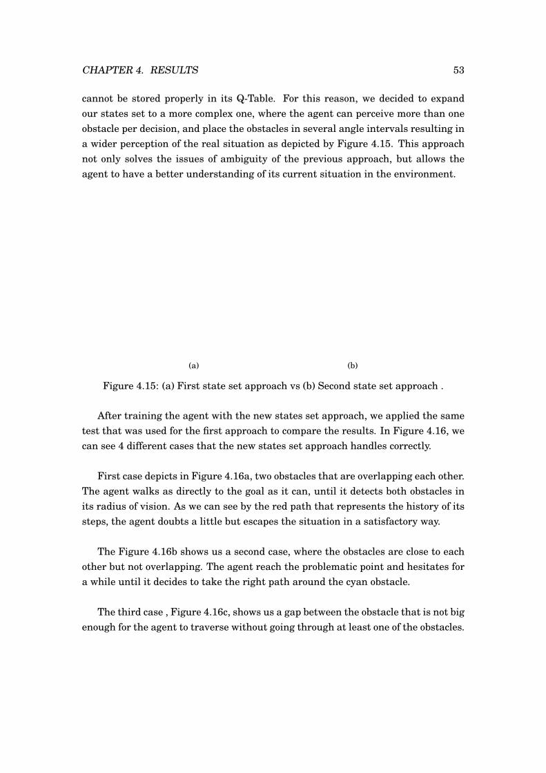
CHAPTER 4. RESULTS 53
cannot be stored properly in its Q-Table. For this reason, we decided to expandour states set to a more complex one, where the agent can perceive more than oneobstacle per decision, and place the obstacles in several angle intervals resulting ina wider perception of the real situation as depicted by Figure 4.15. This approachnot only solves the issues of ambiguity of the previous approach, but allows theagent to have a better understanding of its current situation in the environment.
(a) (b)
Figure 4.15: (a) First state set approach vs (b) Second state set approach .
After training the agent with the new states set approach, we applied the sametest that was used for the first approach to compare the results. In Figure 4.16, wecan see 4 different cases that the new states set approach handles correctly.
First case depicts in Figure 4.16a, two obstacles that are overlapping each other.The agent walks as directly to the goal as it can, until it detects both obstacles inits radius of vision. As we can see by the red path that represents the history of itssteps, the agent doubts a little but escapes the situation in a satisfactory way.
The Figure 4.16b shows us a second case, where the obstacles are close to eachother but not overlapping. The agent reach the problematic point and hesitates fora while until it decides to take the right path around the cyan obstacle.
The third case , Figure 4.16c, shows us a gap between the obstacle that is not bigenough for the agent to traverse without going through at least one of the obstacles.

CHAPTER 4. RESULTS 54
The agent successfully avoids going into that absorbing state and continues its wayto the goal.
Finally in our fourth case shown in Figure 4.16d, there is a gap just big enoughfor the agent to squeeze in. So far, this has been the case that takes the agentlonger to evaluate. After a higher amount of steps than before, as it can be seen onthe red path, the agent manages to fit through the gap and walk straight to the goal.
(a) (b)
(c) (d)
Figure 4.16: Second state set approach twins test: (a) Overlapping obstacles, (b)Close obstacles, (c) Not enough space for the agent to walk through and (d) Tight fitfor the agent to walk through.
These results indicate that the change from state set approach was effective tohandle the issues brought by the inclusion of more obstacles in the simulation. Thiswas an imperative problem because, in our learning problem, other agents are con-sidered as obstacles as well.

CHAPTER 4. RESULTS 55
4.3 Visual results.
To demonstrate the versatility of our reinforcement learning model, we thought ofdifferent scenarios where it would be interesting to prove the knowledge acquire bythe agent during training. We improved the Q-Table from the previous results bysubjecting it to a more thorough training process. It was necessary to fill the stateswhere several objects can be detected before subjecting the Q-Table to a trial in acrowd simulation.
(a) (b)
(c) (d)
Figure 4.17: Single agent in field of dummies.
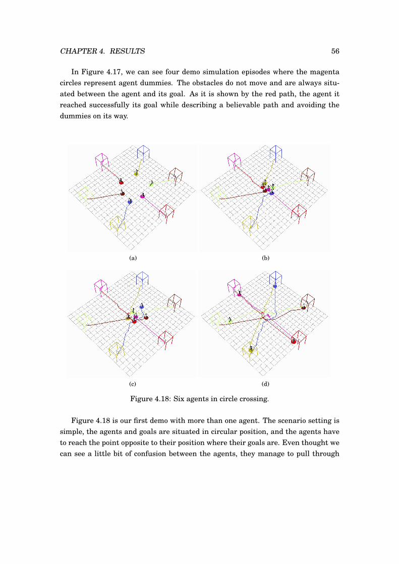
CHAPTER 4. RESULTS 56
In Figure 4.17, we can see four demo simulation episodes where the magentacircles represent agent dummies. The obstacles do not move and are always situ-ated between the agent and its goal. As it is shown by the red path, the agent itreached successfully its goal while describing a believable path and avoiding thedummies on its way.
(a) (b)
(c) (d)
Figure 4.18: Six agents in circle crossing.
Figure 4.18 is our first demo with more than one agent. The scenario setting issimple, the agents and goals are situated in circular position, and the agents haveto reach the point opposite to their position where their goals are. Even thought wecan see a little bit of confusion between the agents, they manage to pull through
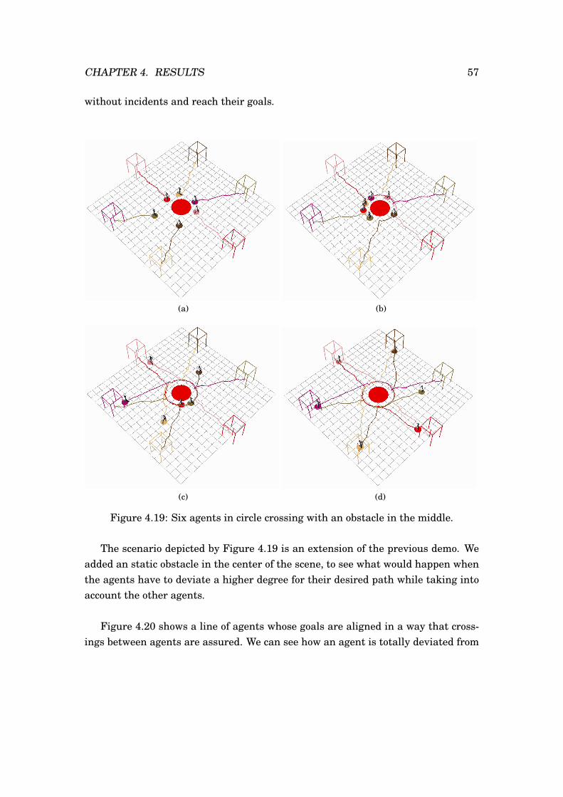
CHAPTER 4. RESULTS 57
without incidents and reach their goals.
(a) (b)
(c) (d)
Figure 4.19: Six agents in circle crossing with an obstacle in the middle.
The scenario depicted by Figure 4.19 is an extension of the previous demo. Weadded an static obstacle in the center of the scene, to see what would happen whenthe agents have to deviate a higher degree for their desired path while taking intoaccount the other agents.
Figure 4.20 shows a line of agents whose goals are aligned in a way that cross-ings between agents are assured. We can see how an agent is totally deviated from

CHAPTER 4. RESULTS 58
(a) (b)
(c) (d)
Figure 4.20: Six agents in line crossing.
its original course, but still manages to find a coherent way to its goal after it is freefrom possible collision conflicts.
The next simulation, shown in Figure 4.21, is an extension from the previousone. We introduced a moving obstacle to check that the agents were able to avoid iteven while trying to maintain an efficient path to their respective goals.
Another setting tried was assigning the same goal for each agent in the simula-
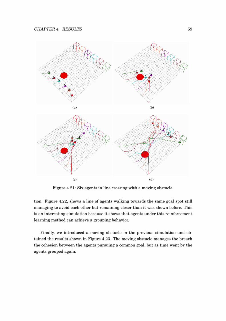
CHAPTER 4. RESULTS 59
(a) (b)
(c) (d)
Figure 4.21: Six agents in line crossing with a moving obstacle.
tion. Figure 4.22, shows a line of agents walking towards the same goal spot stillmanaging to avoid each other but remaining closer than it was shown before. Thisis an interesting simulation because it shows that agents under this reinforcementlearning method can achieve a grouping behavior.
Finally, we introduced a moving obstacle in the previous simulation and ob-tained the results shown in Figure 4.23. The moving obstacle manages the breachthe cohesion between the agents pursuing a common goal, but as time went by theagents grouped again.
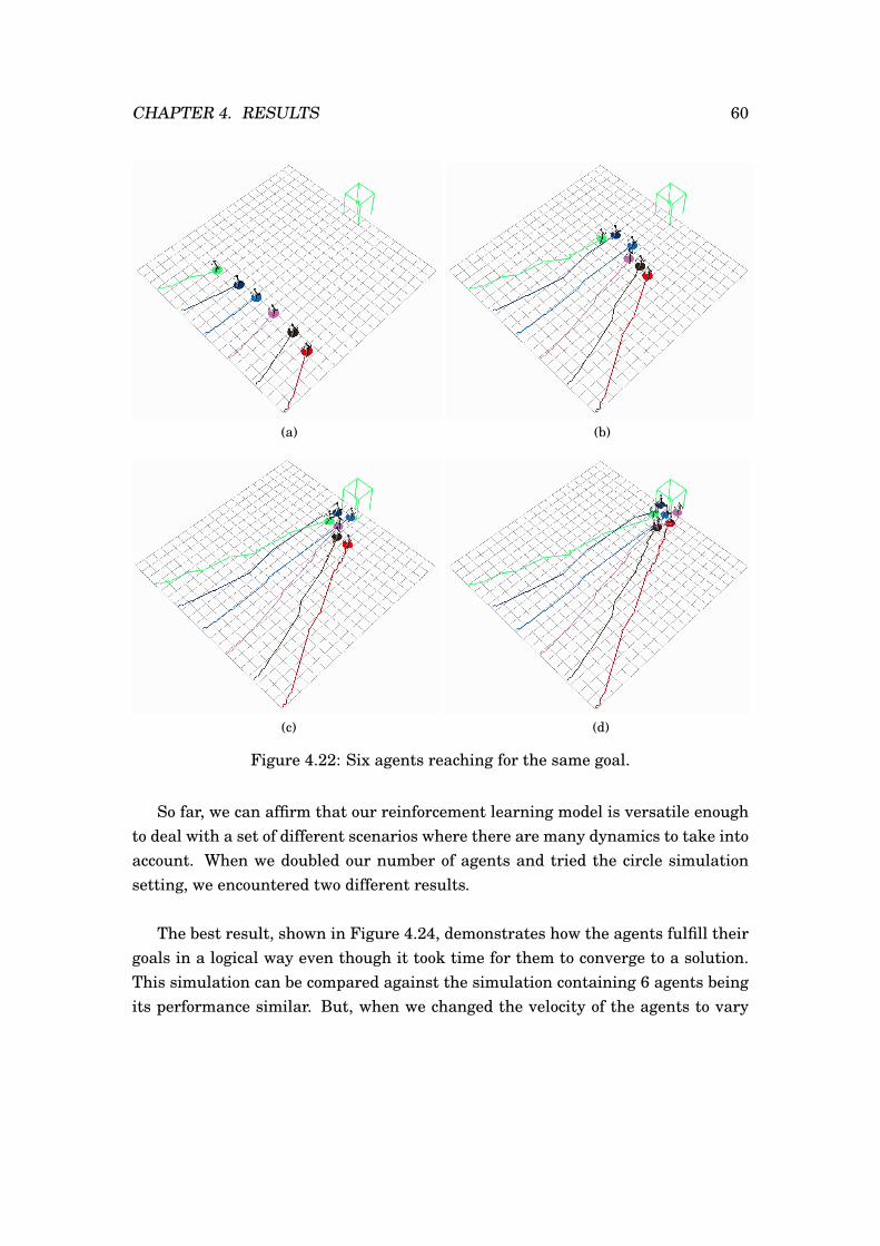
CHAPTER 4. RESULTS 60
(a) (b)
(c) (d)
Figure 4.22: Six agents reaching for the same goal.
So far, we can affirm that our reinforcement learning model is versatile enoughto deal with a set of different scenarios where there are many dynamics to take intoaccount. When we doubled our number of agents and tried the circle simulationsetting, we encountered two different results.
The best result, shown in Figure 4.24, demonstrates how the agents fulfill theirgoals in a logical way even though it took time for them to converge to a solution.This simulation can be compared against the simulation containing 6 agents beingits performance similar. But, when we changed the velocity of the agents to vary
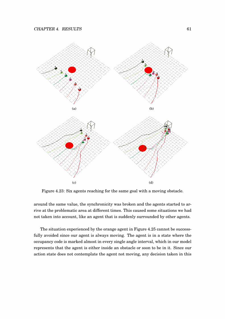
CHAPTER 4. RESULTS 61
(a) (b)
(c) (d)
Figure 4.23: Six agents reaching for the same goal with a moving obstacle.
around the same value, the synchronicity was broken and the agents started to ar-rive at the problematic area at different times. This caused some situations we hadnot taken into account, like an agent that is suddenly surrounded by other agents.
The situation experienced by the orange agent in Figure 4.25 cannot be success-fully avoided since our agent is always moving. The agent is in a state where theoccupancy code is marked almost in every single angle interval, which in our modelrepresents that the agent is either inside an obstacle or soon to be in it. Since ouraction state does not contemplate the agent not moving, any decision taken in this
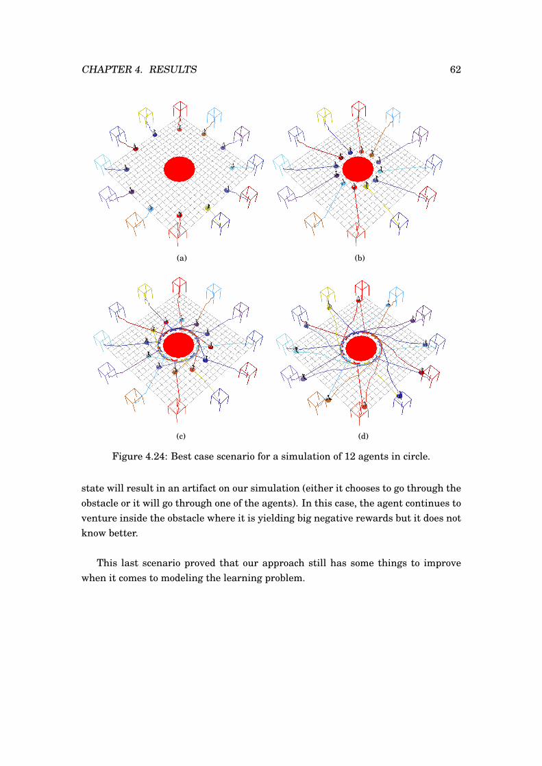
CHAPTER 4. RESULTS 62
(a) (b)
(c) (d)
Figure 4.24: Best case scenario for a simulation of 12 agents in circle.
state will result in an artifact on our simulation (either it chooses to go through theobstacle or it will go through one of the agents). In this case, the agent continues toventure inside the obstacle where it is yielding big negative rewards but it does notknow better.
This last scenario proved that our approach still has some things to improvewhen it comes to modeling the learning problem.

CHAPTER 4. RESULTS 63
(a) (b)
(c) (d)
Figure 4.25: Worst case scenario for a simulation of 12 agents in circle.
Chapter 5
Conclusions
We will now present the conclusions reached during our work both regarding ourmodel and the reinforcement learning requirements. To close this chapter, we pro-pose some improvements needed over our current approach to solve some issuesinherent to it.
5.1 Conclusions
The reward function evaluation showed us the importance of a unambiguous re-ward function. If we want the agent to achieve our goals, these have to be clearlyexpressed in terms of positive rewards and penalties so the agent cannot make in-correct assumptions of what we are asking it to perform. Another important thingobserved during the evaluation, is how the preliminary results during training donot necessarily depict the final results, but are just a guide to measure what theagent is learning. During training, the agent follows an ε-greedy policy that intro-duce randomness in its action selection. These partial results could be consideredas projections of what the agent could achieve. The visual results during trainingshould improve over time, otherwise there are problems with the definition of theRL elements and no amount of training can correct that.
Regarding the training process, it has to be taken into account that the agentwill learn only from the situations it experiences. The training process has to bethorough enough to allow the agent to experience several times different settings.This group of scenarios need to comprise all the states set the agent is using, so theagent is able to improve its decisions over time. An incomplete Q-Table can provide
64

CHAPTER 5. CONCLUSIONS 65
believable results for states that have been visited several times but for those whowere not lucky enough could present poor action selection.
Our model proved to fulfill our goals to a certain degree, but failed to representin certain situations resulting in artifacts in our simulation. Despite its weak-nesses, this work proves once again that Reinforcement Learning methods are avalid option for modeling crowd simulations, given its flexibility and adaptive char-acteristics. Once the learning problem is properly defined, the work of the animatoris done and the training process can begin, resulting in a compilation of experiencesthat can be used for any amount of characters desired in a simulation.
5.2 Future Work
As future work, there are a few subjects we think would be reasonable to explore.For instance, the introduction of an action that means to stay put and not movein any direction. Our work does not contemplate the agents choosing not to move,hence we obtained some artifacts when everyone around it is moving and the agentis trapped (the agent will go through another agent or obstacle). This is a trickydecision because it introduces a new problem into the reward function. It has to bedefined some sort of time penalization or a way to express that staying in the samestate for too long is not always good or this action could be valuated as the go-toaction, just because it has no penalization and that could be considered as a goodreward.
Another matter to attend would be on the crowd controller module. The infor-mation fed to the agent is recollected by checking all the obstacles/agents in thescenario to see which ones are inside the agent’s radius of vision. With an unsortedlist of obstacles/agents, the states are defined but there is no differentiation betweenan obstacle an another one in this step, all we are focused on is in stating that thereis something on the agent’s way to certain intervals of distance. Hence, in the worstcase scenario, if we have a long radius of vision and all the objects on the list arealigned in a queue, hey are all going to be checked in the state construction, eventhough it is possible that the state could have been defined just by a few of them.To solve this issue, we propose to work in the perception of the environment as it isthe perception of a human. Meaning avoiding to add to this list , objects that arefully occluded or partially occluded (if the part that is perceived is occluded but not

CHAPTER 5. CONCLUSIONS 66
the object as a whole).
Finally, our proposed set of states is thought to resume every single possiblesituation that might occur during simulation but this comes with a cost that couldbe avoided. In order to get a believable simulation, there has to be a learning periodwhere we try to mimic the scenarios that could occur. With a bigger amount of statesthere are more scenarios that we have to make sure that are tried before going intoa “demo” version of the Q-Table. For this reason, it is highly encouraged to workon the set of states to achieve a more condensed one (e.g. Nearest distance to theagent could be considered as a whole circle and not slices), but this has proven tobe a delicate subject because changes in the set state could mean changes in thereward function calculation.
Bibliography
[1] Thalmann,C ,and Raupp M, S (2007): Crowd Simulation. Springer-Verlag,London.
[2] Pelechano, N., Allbeck, J and Bardler, N (2008): Virtual Crowds: Methods,Simulation, and Control. Synthesis Lectures on Computer Graphics and Ani-mation #8, Morgan and Claypool Publishers.
[3] Duives, D.C., Daamen, W. and Hoogendoorn, S.P. (2013): State-of-the-artcrowd motion simulation models. Transportation Research Part C: EmergingTehcnologies, 37,193-209.
[4] Helbing, D and Molnar,P: (1995): Social Force Model for Pedestrian Dynamics.Physical review E, 51(5),4282.
[5] Moussaïd, M., Perozo, N., Garnier, S., Helbing, D., and Theraulaz, G. (2010):The walking behaviour of pedestrian social groups and its impact on crowddynamics. PloS one, 5(4), e10047.
[6] Shukla, P. K. (2010): On modeling and evolutionary optimization of nonlin-early coupled pedestrian interactions. In Applications of Evolutionary Compu-tation (pp. 21-30). Springer Berlin Heidelberg.
[7] Dutra, T. B., Cavalcante-Neto, J. B., and Vidal, C. A. (2011): A hybrid model forsimulating crowd with varied behaviors in real-time. In Virtual Reality (SVR),2011 XIII Symposium on (pp. 232-241). IEEE.
[8] Saboia, P., and Goldenstein, S. (2011): Crowd Simulation: Improving Pedestri-ans’ Dynamics by the Application of Lattice-Gas Concepts to the Social ForceModel. In Graphics, Patterns and Images (Sibgrapi), 2011 24th SIBGRAPIConference on (pp. 41-47). IEEE.
67
BIBLIOGRAPHY 68
[9] Zanlungo, F., Ikeda, T., & Kanda, T. (2011): Social force model with explicitcollision prediction. EPL (Europhysics Letters), 93(6), 68005
[10] Gao, Y., Luh, P. B., Zhang, H., & Chen, T. (2013): A modified social force modelconsidering relative velocity of pedestrians. In Automation Science and Engi-neering (CASE), 2013 IEEE International Conference on (pp. 747-751). IEEE.
[11] Yan, G. W., Li, C. Q., & Mu-chao, L. (2012): A novel swarm optimization al-gorithm based on Social Force model for multimodal functions. In Control andDecision Conference (CCDC), 2012 24th Chinese (pp. 849-854). IEEE.
[12] Li, Z., and Jiang, Y. (2012): A Friction Based Social Force Model for GroupBehaviors. In Proceedings of the The 2012 IEEE/WIC/ACM International JointConferences on Web Intelligence and Intelligent Agent Technology-Volume 02(pp. 1-8). IEEE Computer Society.
[13] Jiahui, W., and Jie, S. (2013, November): Emergency evacuation in subwaystation based on Combined Social Force Model. In Electronics Information andEmergency Communication (ICEIEC), 2013 IEEE 4th International Confer-ence on (pp. 242-245). IEEE.
[14] Dijkstra,J., Timmermans, H.J. and Jessurun, A.J (2001): A multi-agent cellu-lar automata system for visualising simulated peestria activity. In Theory andPractical Issues on Cellular Automata (pp.29-36). Springer London.
[15] Sarmady, S., Haron, F., and Talib, A. Z. (2010): Simulating crowd movementsusing fine grid cellular automata. In Computer Modelling and Simulation (UK-Sim), 2010 12th International Conference On (pp. 428-433). IEEE.
[16] Zhang, S., Li, M., Li, F., Liu, A., and Cai, D. (2011): A simulation model ofpedestrian flow based on geographical cellular automata. In Geoinformatics,2011 19th International Conference on (pp. 1-5). IEEE. Chicago.
[17] Zhiqiang, K., Chongchong, Y., Li, T., and Jingyan, W. (2011): Simulation ofevacuation based on multi-agent and cellular automaton. In Mechatronic Sci-ence, Electric Engineering and Computer (MEC), 2011 International Confer-ence on (pp. 550-553). IEEE.
[18] Long, L. W., Hua, W. Y., Ping, L., and YingJie, W. (2011): Research on cellu-lar automaton model for evacuation under passenger station. In Electronics,

BIBLIOGRAPHY 69
Communications and Control (ICECC), 2011 International Conference on (pp.4465-4468). IEEE. Chicago.
[19] Zainuddin, Z., and Aik, L. E. (2012): Refined cellular automata model forTawaf simulation. In Computers & Informatics (ISCI), 2012 IEEE Symposiumon (pp. 46-51). IEEE.
[20] Carneiro, L. D. O., Cavalcante-Neto, J. B., Vidal, C. A., and Dutra, T. B. (2013):Crowd Evacuation Using Cellular Automata: Simulation in a Soccer Stadium.In Virtual and Augmented Reality (SVR), 2013 XV Symposium on (pp. 240-243). IEEE.
[21] Ben, X., Huang, X., Zhuang, Z., Yan, R., and Xu, S. (2013): Agent-based ap-proach for crowded pedestrian evacuation simulation. Intelligent TransportSystems, IET, 7(1), 56-67
[22] Chang, J. (2013): Simulation of Personnel Evacuation Based on Cellular Au-tomata: To Consider Individual Character and Following Behavior. In Com-putational Intelligence and Design (ISCID), 2013 Sixth International Sympo-sium on (Vol. 2, pp. 403-405). IEEE.
[23] Chang, J. (2013): Evacuation Simulation Based on 2.5 D Cellular Automata:To Consider Individual Character and Following Behavior. In Computer Sci-ences and Applications (CSA), 2013 International Conference on (pp. 288-291).IEEE.
[24] Giitsidis, T., & Sirakoulis, G. C. (2014): Simulation of aircraft disembarkingand emergency evacuation. In Parallel, Distributed and Network-Based Pro-cessing (PDP), 2014 22nd Euromicro International Conference on (pp. 372-379). IEEE
[25] Reynolds ,C.W(1987): Flocks, herds and schools: A distributed behavioralmodel. In Computer Graphics, Volume 21, Number 4, ACM, pp.25-34.
[26] Xiong, J., Wang, J., Yang, K., Peng, S., and Xu, Q. (2010): Multiagent-basedsimulation of the HIV/AIDS spatial and temporal transmission among injec-tion drug users. In Geoinformatics, 2010 18th International Conference on (pp.1-6). IEEE. Chicago
[27] Wulansari, O. D. E. (2010): Steering behavior analysis and implementation tosimulate crowd tawaf ritual on Augmented Reality Manasik. In Distributed

BIBLIOGRAPHY 70
Framework and Applications (DFmA), 2010 International Conference on (pp.1-7). IEEE.
[28] Kumarage, D., Wimalaratne, P., and Ranawana, R. (2011): Simulated hornetattack on crowd in a virtual environment. In VR Innovation (ISVRI), 2011IEEE International Symposium on (pp. 55-62). IEEE.
[29] Reynolds, Craig. (2004):"Opensteer: Steering behaviors for autonomous char-acters." Website.[Available: http://opensteer. sourceforge. net] .
[30] Sun, L., and Qin, W. (2011). Simulation of crowd behaviors based on event re-action. In Computer Science and Automation Engineering (CSAE), 2011 IEEEInternational Conference on (Vol. 2, pp. 163-167). IEEE.
[31] Yu, L., and Duan, C. (2011). Evacuation modelling: An agent based ap-proach. In Artificial Intelligence, Management Science and Electronic Com-merce (AIMSEC), 2011 2nd International Conference on (pp. 7080-7083).IEEE.
[32] Yuan, Y., Wu, Z., and Zhou, M. (2012): Populating virtual environments withcrowd patches and rule-based method. In Proceedings of the 11th ACM SIG-GRAPH International Conference on Virtual-Reality Continuum and its Ap-plications in Industry (pp. 239-246). ACM.
[33] Zhong, J., Luo, L., Cai, W., & Lees, M. (2014): Automatic rule identifica-tion for agent-based crowd models through gene expression programming.In Proceedings of the 2014 international conference on Autonomous agentsand multi-agent systems (pp. 1125-1132). International Foundation for Au-tonomous Agents and Multiagent Systems.
[34] Torrey, L. (2010): Crowd Simulation Via Multi-Agent Reinforcement Learning.In AIIDE.
[35] Lee, S. J., and Popovic, Z. (2010): Learning behavior styles with inverse rein-forcement learning. ACM Transactions on Graphics (TOG), 29(4), 122.
[36] Cuayáhuitl, H., Dethlefs, N., Frommberger, L., Richter, K. F., and Bateman,J. (2010): Generating adaptive route instructions using hierarchical reinforce-ment learning. In Spatial Cognition vii (pp. 319-334). Springer Berlin Heidel-berg.

BIBLIOGRAPHY 71
[37] Martinez-Gil, F., Barber, F., Lozano, M., Grimaldo, F., and Fernández, F.(2010): A Reinforcement Learning Approach for Multiagent Navigation. InICAART (1) (pp. 607-610).
[38] Kastanis, I., and Slater, M. (2012): Reinforcement learning utilizes proxemics:An avatar learns to manipulate the position of people in immersive virtualreality. ACM Transactions on Applied Perception (TAP), 9(1), 3.
[39] Martinez-Gil, F., Lozano, M., and Fernández, F. (2012):Calibrating a motionmodel based on reinforcement learning for pedestrian simulation. In Motionin Games (pp. 302-313). Springer Berlin Heidelberg.
[40] Lo, W. Y., Knaus, C., and Zwicker, M. (2012): Learning motion con-trollers with adaptive depth perception. In Proceedings of the ACM SIG-GRAPH/Eurographics Symposium on Computer Animation (pp. 145-154). Eu-rographics Association.
[41] Rothkopf, C. A., and Ballard, D. H. (2013): Modular inverse reinforcementlearning for visuomotor behavior. Biological cybernetics, 107(4), 477-490.
[42] Hao, J., and Leung, H. F. (2013): Achieving socially optimal outcomes in mul-tiagent systems with reinforcement social learning. ACM Transactions on Au-tonomous and Adaptive Systems (TAAS), 8(3), 15.
[43] Martinez-Gil, F., Lozano, M., and Fernández, F. (2012): Multi-agent reinforce-ment learning for simulating pedestrian navigation. In Adaptive and LearningAgents (pp. 54-69). Springer Berlin Heidelberg.
[44] Martinez-Gil, F., Lozano, M., and Fernández, F. (2014): Strategies for sim-ulating pedestrian navigation with multiple reinforcement learning agents.Autonomous Agents and Multi-Agent Systems, 1-33.
[45] Beheshti, R., and Sukthankar, G. (2014): A normative agent-based model forpredicting smoking cessation trends. In Proceedings of the 2014 internationalconference on Autonomous agents and multi-agent systems (pp. 557-564). In-ternational Foundation for Autonomous Agents and Multiagent Systems.
[46] Kaelbling,L.P, Littman, M.L, and Moore, A.W.(1996): Reinforcement learning:A survey. arXiv preprint cs/9605103.

BIBLIOGRAPHY 72
[47] Sutton, R.S an Barto, A.G. (1998): Introduction to reinforcement learning. MITPress.
[48] Watkins, C. J., and Dayan, P. (1992): Q-learning. Machine learning, 8(3-4),279-292.

73