Social and Cognitive Peer Effects:Experimental Evidence from Selective High Schools in Peru

Roman Andres Zarate∗

January 23, 2019

Job Market PaperPlease find the latest version here.

AbstractA growing literature emphasizes the importance of social skills in the labor market.

However, to date, no study addresses the role of peer characteristics in the formationof social skills. This paper reports estimates of cognitive and social peer effects froma large-scale field experiment at selective boarding schools in Peru. My experimen-tal design overcomes some methodological challenges in the peer effects literature. Irandomly varied the characteristics of neighbors in dormitories with two treatments:(a) less or more sociable peers (identified by their position in the school’s friendshipnetwork before the intervention) and (b) lower- or higher-achieving peers (identifiedby admission test scores). While more sociable peers enhance the formation of socialskills, higher-achieving peers do not improve academic achievement; in fact, they fur-ther reduce the academic performance of lower-achieving students. These results ap-pear to be driven by students’ self-confidence and the social support they receive fromtheir neighbors. I interpret these findings in the context of a simple self-confidencemodel where students infer their skills by interacting with their peers.

∗Department of Economics, MIT. Email: razarate@mit.edu. I am deeply grateful to my advisors Joshua Angrist, Esther Duflo,and Parag Pathak for their guidance throughout this project. I also thank Daron Acemoglu, Abhijit Banerjee, and Frank Schilbachfor their helpful suggestions. This paper would not have been possible without the support of the staff of the Ministry Educationof Peru; I especially thank Marıa Antonieta Alva and Cinthia Wicht for their collaboration and support, and Paola Encalada for herdedicated work at different stages of this project. I also thank Andrei Bartra, Pıa Basurto, Antonio Campos, Jose Carlos Chavez,Yessenia Collahua, Gerald Eliers, Fiorella Guevara, Diego Jara, Ricardo Montero, Raul Panduro, Barbara Sparrow, Guillermo Trefolgi,and Paola Ubillus for their help. I am also grateful to all the directors of the COAR Network for their work during the implementation.Heather McCurdy provided generous help with MIT Institutional Review Board (IRB) documentation. I am particularly gratefulto Sydnee Caldwell, Joaquın Klot, Matt Lowe, and Francine Loza for their feedback. Claudia Allende, Zach Brown, Alonso Bucarey,Adriana Camacho, Lorena Caro, Nicolas de Roux, Josh Dean, Juan Dubra, Leopoldo Fergusson, David Figlio, Chishio Furukawa, IsabelHincapie, Nicolas Idrobo, Juan Galan, Arda Gitmez, Gabriel Kreindler, Stephanie Majerowicz, Santiago Melo, Mateo Montenegro,Andres Moya, Alan Olivi, Gautam Rao, Cory Smith, Vira Semenova, Roman David Zarate, David Zarruk, and the participants at theDevelopment, Labor, Organizational lunches at MIT, NEUDC 2018, and the 2018 NAEd/Spencer fellows retreat also provided usefulcomments and suggestions. Jorge Alva and Marıa Antonieta Luperdi were very generous during my stay in Peru. This project is partof the MineduLab. Funding for this project was generously provided by the Weiss Family Fund and the NAEd/Spencer dissertationfellowship. The experiment was approved by the MIT IRB (ID 1702862092), and is registered at the AEA RCT Registry (ID 0002600).

1

1 Introduction

Social skills are a determinant of individuals’ well-being and labor market success. For in-stance, social skills are important for communication within organizations and team pro-ductivity (Woolley et al., 2010; Adhvaryu et al., 2018). They facilitate interactions betweenpeople, and thus cannot be easily substituted by automation (Autor, 2014). Recent em-pirical evidence shows that the labor market increasingly rewards social skills (Deming,2017), and that social skills are complementary to cognitive skills (Weinberger, 2014). De-spite this recognition there is little research in economics on how social skills are formed.

Policymakers may be able to use peer effects to influence the formation of social skills.Intuitively, students could develop these skills by interacting with highly sociable peers.Sociable students may also affect the formation of their peers’ cognitive skills. For exam-ple, it may be easier for students to befriend sociable peers, and having more friends im-proves academic achievement (Lavy and Sand, 2012). Likewise, some evidence suggeststhat students benefit from being in school with higher-achieving peers but only whenthey are in fact studying together (Carrell et al., 2013). Therefore, peers’ social and cogni-tive skills could have complementary effects on academic achievement. While economistsas other social scientists have extensively studied peer effects on academic achievement,behaviors, and racial attitudes (Epple and Romano, 2011; Sacerdote, 2011; Boisjoly et al.,2006), to my knowledge there is no research in Economics of the impact of peers’ sociabilityon the formation of cognitive or social skills.

This paper reports estimates of social and cognitive peer effects from a large-scale fieldexperiment at selective boarding schools in Peru. While other studies have exploited ran-dom assignment to dormitories and classrooms—relying only in randomly occuring vari-ation in peer characteristics—I use a novel experimental design to generate large varia-tion in peer skills. Specifically, I assign students to two cross-randomized treatments inthe allocation to beds in a dormitory: (1) less or more sociable peers, and (2) lower- orhigher-achieving peers. This design surmounts many of the challenges with traditionalapproaches to study peer effects, which have suffered from a version of weak instrumentsor other biases (Manski, 1993; Angrist, 2014; Caeyers and Fafchamps, 2016).

To classify students as less vs. more sociable, I collected data on the social networksthe year before the intervention. I asked students who were their preferred neighbors,their friends, and with whom do they study or play. I construct an aggregate networkwith the four questions and use eigenvector centrality as a measure of sociability. Thismeasure accounts for the fact that high central individuals are connected to other highcentral individuals as well. In the context of my study, this indicator is highly correlatedwith other metrics introduced by psychologists to measure social skills. To classify stu-dents as higher vs. lower achieving, I use students’ scores from the schools’ admissionstests, which include math and reading comprehension scores.

2

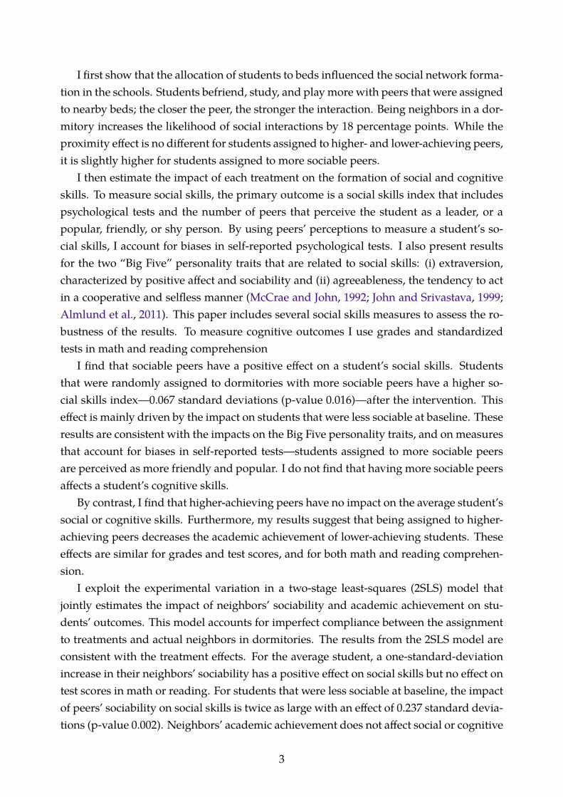
I first show that the allocation of students to beds influenced the social network forma-tion in the schools. Students befriend, study, and play more with peers that were assignedto nearby beds; the closer the peer, the stronger the interaction. Being neighbors in a dor-mitory increases the likelihood of social interactions by 18 percentage points. While theproximity effect is no different for students assigned to higher- and lower-achieving peers,it is slightly higher for students assigned to more sociable peers.

I then estimate the impact of each treatment on the formation of social and cognitiveskills. To measure social skills, the primary outcome is a social skills index that includespsychological tests and the number of peers that perceive the student as a leader, or apopular, friendly, or shy person. By using peers’ perceptions to measure a student’s so-cial skills, I account for biases in self-reported psychological tests. I also present resultsfor the two “Big Five” personality traits that are related to social skills: (i) extraversion,characterized by positive affect and sociability and (ii) agreeableness, the tendency to actin a cooperative and selfless manner (McCrae and John, 1992; John and Srivastava, 1999;Almlund et al., 2011). This paper includes several social skills measures to assess the ro-bustness of the results. To measure cognitive outcomes I use grades and standardizedtests in math and reading comprehension

I find that sociable peers have a positive effect on a student’s social skills. Studentsthat were randomly assigned to dormitories with more sociable peers have a higher so-cial skills index—0.067 standard deviations (p-value 0.016)—after the intervention. Thiseffect is mainly driven by the impact on students that were less sociable at baseline. Theseresults are consistent with the impacts on the Big Five personality traits, and on measuresthat account for biases in self-reported tests—students assigned to more sociable peersare perceived as more friendly and popular. I do not find that having more sociable peersaffects a student’s cognitive skills.

By contrast, I find that higher-achieving peers have no impact on the average student’ssocial or cognitive skills. Furthermore, my results suggest that being assigned to higher-achieving peers decreases the academic achievement of lower-achieving students. Theseeffects are similar for grades and test scores, and for both math and reading comprehen-sion.

I exploit the experimental variation in a two-stage least-squares (2SLS) model thatjointly estimates the impact of neighbors’ sociability and academic achievement on stu-dents’ outcomes. This model accounts for imperfect compliance between the assignmentto treatments and actual neighbors in dormitories. The results from the 2SLS model areconsistent with the treatment effects. For the average student, a one-standard-deviationincrease in their neighbors’ sociability has a positive effect on social skills but no effect ontest scores in math or reading. For students that were less sociable at baseline, the impactof peers’ sociability on social skills is twice as large with an effect of 0.237 standard devia-tions (p-value 0.002). Neighbors’ academic achievement does not affect social or cognitive

3

outcomes, on average. However, for lower-achieving students, a one-standard-deviationincrease in their neighbors’ academic scores leads to a reduction in math and readingscores of 0.082 (p-value 0.081) and 0.122 (p-value 0.040) standard deviations, respectively.

My results are twofold. First, I provide evidence that, for less sociable students, ex-posure to more sociable peers has a positive effect on social skills. Second, I find thatexposure to higher-achieving peers does not positively influence academic achievement;there is evidence suggesting that they further decrease the academic achievement of lowachievers. Therefore, my main conclusion is that while sociable peers make you more sociable,higher-achieving peers do not improve your academic learning.

I then explore the potential mechanisms that drive my results. I examine whether thechange in students’ self-confidence in their skills is a valid mechanism. First, I show thatmy results are consistent with a simple model of self-confidence based on Compte andPostlewaite (2004). Second, I provide suggestive empirical evidence that changes in self-confidence explain my findings.

The idea behind the model is that, while more sociable peers make less sociable stu-dents feel better about their social skills, higher-achieving peers make lower achievingstudents feel worse about their cognitive skills. Under this framework, success in social orcognitive activities is a function of self-confidence, and self-confidence depends on pastsuccesses. It is easier for less sociable students to engage in social activities with more—rather than less—sociable peers, and these interactions make students more successful.Success translates into more self-confidence in social skills, making students more likelyto do well in future interactions with both neighbors and other people. By contrast, lower-achieving students feel less accomplished when assigned to higher-achieving peers. If stu-dents think they are doing worse, they are less confident in their academic skills, drivingdown their investment in cognitive activities.

I find empirical evidence consistent with self-confidence driving my results. First, lesssociable students report better social interactions with their neighbors when assigned tomore sociable peers. In particular, they are happier with their dormitory assignments,and indicate that their neighbors are more empathetic towards them. Likewise, there isevidence suggesting that less sociable students gain self-confidence in their social skillswhen assigned to more sociable peers. By contrast, lower-achieving students report lessself-confidence in their cognitive abilities when assigned to higher-achieving peers.

I also rule out the possibility that the number of social interactions between studentsand their neighbors is driving the empirical findings as in Carrell et al. (2013). I exploretwo questions to reach this conclusion: (1) do less sociable students have more social inter-actions with their peers when assigned to more sociable peers?, and (2) do lower-achievingstudents interact less with their peers when assigned to higher-achieving peers? I find ev-idence against both hypotheses. Less sociable students have a similar number of socialinteractions with their peers, regardless of their random assignment to the more sociable

4

peers treatment. Likewise, although lower-achieving students are studying with higher-achieving peers, they still experience declines in academic achievement.

This paper builds on and contributes to three strands of the literature: (i) the formationof social skills, (ii) social networks, and (iii) the identification and consequences of peereffects.

My results explore how peer characteristics affect the development of social skills inschool, extending the literature on the formation of social skills. While a substantial bodyof evidence documents positive and increasing returns to social skills in the labor mar-ket (Deming, 2017), little is known about how social skills are formed. There are a fewexceptions: Rao (2013) shows that rich students are more altruistic and discriminate lesswhen they are exposed to poor peers. Similarly, Falk et al. (2018) find that a mentorshipprogram in Germany increased children’s pro-sociality. Adhvaryu et al. (2018) show thatan on-the-job soft skills training program in India increased female workers’ extraversionand communication. Finally, there is some evidence of how income (Akee et al., 2018) andincentives (Donato et al., 2017) might affect the Big Five personality traits.1

This paper also builds on the literature on social networks. While some evidence high-lights the role of eigenvector centrality for the diffusion of microfinance (Banerjee et al.,2013) and the monitoring of savings decisions (Breza and Chandrasekhar, 2018), this pa-per confirms that eigenvector centrality is correlated with social skills as measured by psy-chological tests. Moreover, my results show that having highly central peers has a positiveeffect on a student’s social skills.

My experimental design and results reconcile some of the evidence in the peer effectsliterature. Most previous empirical studies of peer effects focus on baseline test scores ofpeers, and employ one of two methodologies for identification: they exploit either the ran-dom formation of groups or quasi-experimental variation in the skills of peers. Studiesthat use the former method find small positive peer effects in small groups such as dormi-tories (Epple and Romano, 2011; Sacerdote, 2001), and sizeable significant effects in largegroups such as classrooms (Duflo et al., 2011), squadrons (Carrell et al., 2009), or large-size dormitories (Garlick, 2018). Golsteyn et al. (2017) also use a similar research design toshow that students perform better in the presence of more persistent and more risk-aversepeers. Studies that employ the second approach use exogenous variation in peer charac-teristics. For example, Abdulkadiroglu et al. (2014) use school-specific admission cutoffsto estimate peer effects in exam schools in Boston and New York, and Duflo et al. (2011)use cutoffs from a tracking system to estimate peer effects in Kenya. In contrast to studiesthat use random allocation to groups, quasi-experimental studies have found zero peereffects.2

1The Big Five personality traits are: openness to experience, conscientiousness , extraversion, agreeable-ness, and emotional stability.

2Garlick (2018) finds a negative impact of tracking for low-scoring students in a university in South Africa.He argues that this result is attributable to peer effects. However, as the author points out, the research

5

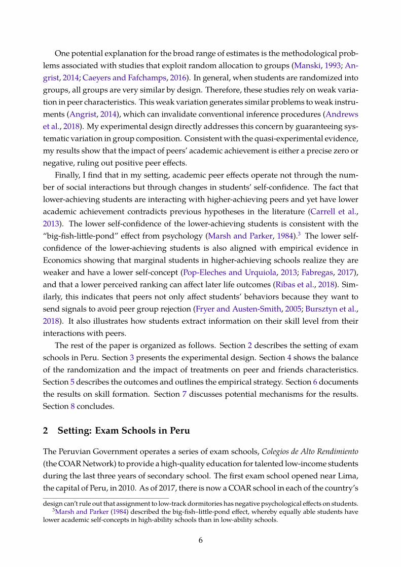
One potential explanation for the broad range of estimates is the methodological prob-lems associated with studies that exploit random allocation to groups (Manski, 1993; An-grist, 2014; Caeyers and Fafchamps, 2016). In general, when students are randomized intogroups, all groups are very similar by design. Therefore, these studies rely on weak varia-tion in peer characteristics. This weak variation generates similar problems to weak instru-ments (Angrist, 2014), which can invalidate conventional inference procedures (Andrewset al., 2018). My experimental design directly addresses this concern by guaranteeing sys-tematic variation in group composition. Consistent with the quasi-experimental evidence,my results show that the impact of peers’ academic achievement is either a precise zero ornegative, ruling out positive peer effects.

Finally, I find that in my setting, academic peer effects operate not through the num-ber of social interactions but through changes in students’ self-confidence. The fact thatlower-achieving students are interacting with higher-achieving peers and yet have loweracademic achievement contradicts previous hypotheses in the literature (Carrell et al.,2013). The lower self-confidence of the lower-achieving students is consistent with the“big-fish-little-pond” effect from psychology (Marsh and Parker, 1984).3 The lower self-confidence of the lower-achieving students is also aligned with empirical evidence inEconomics showing that marginal students in higher-achieving schools realize they areweaker and have a lower self-concept (Pop-Eleches and Urquiola, 2013; Fabregas, 2017),and that a lower perceived ranking can affect later life outcomes (Ribas et al., 2018). Sim-ilarly, this indicates that peers not only affect students’ behaviors because they want tosend signals to avoid peer group rejection (Fryer and Austen-Smith, 2005; Bursztyn et al.,2018). It also illustrates how students extract information on their skill level from theirinteractions with peers.

The rest of the paper is organized as follows. Section 2 describes the setting of examschools in Peru. Section 3 presents the experimental design. Section 4 shows the balanceof the randomization and the impact of treatments on peer and friends characteristics.Section 5 describes the outcomes and outlines the empirical strategy. Section 6 documentsthe results on skill formation. Section 7 discusses potential mechanisms for the results.Section 8 concludes.

2 Setting: Exam Schools in Peru

The Peruvian Government operates a series of exam schools, Colegios de Alto Rendimiento(the COAR Network) to provide a high-quality education for talented low-income studentsduring the last three years of secondary school. The first exam school opened near Lima,the capital of Peru, in 2010. As of 2017, there is now a COAR school in each of the country’s

design can’t rule out that assignment to low-track dormitories has negative psychological effects on students.3Marsh and Parker (1984) described the big-fish–little-pond effect, whereby equally able students have

lower academic self-concepts in high-ability schools than in low-ability schools.

6

25 regions. There are 100 slots per cohort in each school, except for the school in Lima,which has 300.

The COAR Network meets the standards of elite private high schools in Latin Amer-ica, where students have access to all the required inputs for a high-quality education.COAR are boarding schools, deliberately located close to the capital city of each region toreduce daily transportation costs for both families and the government. Upon admission,students receive school materials, uniforms, and a personal laptop for school use. All ofthe schools have a high-quality infrastructure, including a library and excellent scientificlaboratories. Students also have the option of obtaining a world-renowned InternationalBaccalaureate (IB) degree. Teachers are hired outside the public school system and receivehigher salaries. The government covers all the necessary operating expenses, includinglaundry service and food.

Applicants are eligible for admission into COAR if they ranked in the top 10 of theirpublic school cohort in the previous academic year. The admissions process consists oftwo rounds. In the first round, applicants take a written test in reading comprehension andmathematics. The highest-scoring applicants move onto a second round, during whichpsychologists rate them based on two activities: a one-to-one interview, and the observa-tion of peer interactions during a set of tasks. I refer to these scores as the interview andsocial fit scores, respectively. Admissions decisions are determined by a composite scoreof all three tests, by the region of origin, and by the applicant’s school preferences.

Before the experiment, school directors implemented their own individual systems toallocate students to dormitories and classrooms. Most schools attempted to foster multi-cultural diversity by mixing students from different regions within the same dormitory.There was also variation across schools in how they allocated first-year students to class-rooms. Classroom assignment for students in the upper cohorts depends on whether stu-dents apply for the IB degree and the track they choose for this program.

3 Experimental Design

This section presents the experimental design. The objective of the experiment is to esti-mate the impact of peers’ sociability and academic achievement on students’ outcomes. Todo this, it is necessary to ensure systematic variation in peer characteristics across treat-ments. I do so by classifying students into types according to sociability and academicachievement, and by randomizing students into groups with systematic variation in thetype of peer. Thus, there is by design substantial variation in peer characteristics acrossthese groups, surmounting the weak variation problem pointed out by Angrist (2014) inother peer effects studies.

This section is divided as follows. First, I describe the data that was available beforethe intervention. Second, I illustrate how I used this data to classify students according to

7

sociability and academic achievement. Third, I explain how students were randomized togroups with different types of peers, and describe how I used this assignment to allocatestudents to dormitories in the schools. Figure 1 illustrates the project’s timeline.

3.1 Data3.1.1 Administrative Data

Administrative data on student demographics and baseline scores was collected as part ofthe admissions process or from existing government databases. For all students enrolledin the COAR Network in 2017, I have data on admissions test scores in three categories:(i) the written test in math and reading comprehension, (ii) the admissions interview, and(iii) the social fit score determined by a team of psychologists.

In addition, I exploit existing government data to describe students’ socio-demographiccharacteristics. The socio-demographic data I use is employed by the Government of Peruto determine households’ eligibility for national social programs, and is available for 85%of students. It includes whether a student comes from a household classified as poor orextremely poor, and whether they come from a rural area.

Column 1 of Table 1 reports descriptive statistics for students in the COAR Network.Although these schools target students from the public school system, admitted studentshave diverse social and economic backgrounds. For example, 35-37% of the students comefrom poor households, and 20% from extremely poor households. Likewise, 26% of stu-dents come from rural households.

For the 2015-16 cohorts, the Ministry of Education also administered psychologicaltests. Some of these tests incorporate measures of social skills, including emotional in-telligence (Law et al., 2004) and the “Reading the Mind in the Eyes” test (Declerck andBogaert, 2008). Appendix C describes these tests in detail.

3.1.2 Surveys

With the Ministry of Education, we administered an online survey to measure social inter-actions and non-cognitive skills for students in the 2015 and 2016 cohorts. The survey wasconducted in class and on a computer, with a compliance rate above 95% for each school.A team of psychologists in each school was in charge of monitoring the survey.

The survey asked students to list the names of their peers in four distinct categoriesof social interactions: (i) roommate preferences (students were told that their answers tothis question could affect their dormitory assignment), (ii) friends , (iii) study mates, and(iv) people with whom they socialized or engaged in social activities. Appendix Table A.1shows three statistics for each category of the network: total degree, mutual degree, andeigenvector centrality. The average mutual degree is half of (or lower than) the average to-tal degree. For example, when we consider a broad social network that aggregates all four

8

questions about social interactions, students report having 7.02 connections on average, ofwhich only 3.24 are mutual.

The survey also included questions on students’ perception by their peers. Studentswere asked to rank up to five peers in the categories of leadership, friendliness, popular-ity, and shyness. Table A.1 shows descriptive statistics for these variables. On average, astudent was named by 3.48 of her peers as the best leader, by 3.59 as the most friendly, by3.21 as the most popular, and by 2.59 as the shyest.

3.2 Classifying Students According to Academic and Social Skills

I use data from the admissions process and baseline social networks survey to identifymore sociable and higher-achieving students.

I use the test score in the first round of the admissions process—that evaluates stu-dents in math and reading comprehension—to characterize students as lower- or higher-achieving at baseline. This test was taken before students interacted at all. For each school-by-grade-by-gender cell, students above the cell-specific median are classified as higherachieving, and those below the median as lower achieving.

To identify more and less sociable students, I rely on the social networks baseline sur-vey described in the previous section. I use the eigenvector centrality of an aggregateundirected social network that groups the four categories of social interactions describedabove; Banerjee et al. (2013) and Banerjee et al. (2014) perform a similar aggregation. Otherstudies have used eigenvector centrality to measure sociability, predict the diffusion of in-formation in other contexts (Banerjee et al., 2014; Beaman and Dillon, 2018), and showhow more central individuals can do a better job at monitoring savings decisions (Brezaand Chandrasekhar, 2018). I use the same strategy to classify students as lower or higherachieving. That is, students with an eigenvector centrality above the cell-specific medianare classified as more sociable, and those below the cell-specific median as less sociable.Appendix Figure A.2 shows that in the context of exam schools in Peru, eigenvector cen-trality and admissions test scores are positively correlated.

Table A.1 (columns 2 to 5) presents descriptive statistics of the baseline social networksby student type. More sociable students have a better position in the schools’ social net-works, with a larger average degree, mutual degree, and eigenvector centrality for thefour social networks reported (roommate preferences, friends, study mates, and socialpartnerships). For example, in the general network more sociable students have, on av-erage, 4 more connections and 1.4 more mutual connections than less sociable students.More sociable students are also perceived as friendly by 4.6 peers on average, while only2.5 peers perceive less sociable students as friendly.

More interestingly, I also find a large statistically significant correlation of eigenvectorcentrality and my set of indicators of social skills. Appendix Table A.2 reports standard-

9

ized coefficients of an OLS regression of social skills measures4 on the three admissionstest scores, and on the eigenvector centrality of the baseline social network controlling forschool×grade×gender fixed effects. For most of my social skills indicators, eigenvectorcentrality has a stronger correlation than admissions test scores. These results confirmthat individuals who are assessed as very central in the schools’ social networks at base-line also have highly developed social skills.

Since first-year students did not complete the baseline survey in 2016, eigenvector cen-trality at baseline is not available for this cohort. However, in an attempt to identify so-ciable students in this cohort, I use the social-fit test in the admission. In theory, this scorecomprises measures of empathy, leadership, and teamwork. However, by contrast withthe eigenvector centrality, the correlation between the social-fit score and more traditionalsocial skills measures is weak. For this reason, I focus on the higher-achieving peers treat-ment for the first-years. Appendix Tables A.6 and A.7 show that my main results are robustto the inclusion of this treatment.

3.3 Randomization

To estimate the impact of peers’ sociability and academic achievement on students’ out-comes, I randomized students to two treatments: (1) more sociable peers, and (2) higher-achieving peers. In the previous section, I explained how students were classified intomore sociable and higher-achieving students. Here I explain the details of the random-ization.

3.3.1 Peer Group Types

By randomizing the type of peer that students have, instead of the simple randomizationto groups, I assure that students in my study are exposed to peers with different levelsof skills. This is a novel approach and is central to my study. It differs from the moretraditional approach that exploits random assignments to groups; where, by virtue of therandomization, peer characteristics are the same in expectation —although there will besmall variation across groups in the realized sample.

The experimental design accounts for the fact that a student, not only receives a treat-ment, but is also a treatment for her peers. Students were allocated to peer group types inwhich they were matched with peers of their respective treatments. In each peer grouptype, half of the peers are of the same type as the student and the other half of the peersare of the type of her assigned treatment.

For exposition, consider the simple case of two types of students: high and low. Theresearcher is interested in identifying the Average Treatment Effect (ATE) of having high-type peers. With two types of students there are three peer group types: two homogenous

4Some of these variables were collected before or after the intervention. They are described in detail insection 5.1 and Appendix C.

10

groups, composed of individuals of a single type, and a heterogeneous group composedof individuals of both types. The following matrix shows the composition of peer grouptypes:

High LowHigh Group A Group BLow Group B Group C

In this case, there are three potential peer group types:

a) Group A: a group composed of the high type only.

b) Group B: a mixed group, in which half are high-type students and the other half arelow-type students.

c) Group C: a group composed of the low type only.

Notice that, conditional on a student’s type, she can be assigned to a homogenousgroup (Groups A and C), with individuals of her own type, or to a mixed group (GroupB), with individuals of both types.

To illustrate how this generates systematic variation across treatments, compare a high-type student in Group A versus a high-type student in Group B. In Group A, all peers arehigh types, while in Group B half of the peers are high types and the other half are lowtypes. Hence, the difference in the proportion of high-type peers in Group A versus Bis equal to 0.5. The Conditional Average Treatment Effect (CATE) of having high-typepeers conditional on being a high-type student (τi = H)can be identified by the differencebetween high-type students in group A and high-type students in Group B.

CATEH = E [Yi|τi = H,A]− E [Yi|τi = H,B] (1)

Similarly, consider a low-type student in Group B versus a low-type student in GroupC. In Group B, half the peers are high types and the other half are low types, while inGroup C all peers are low-type students. Hence, the difference in the proportion of high-type peers in Group B versus C is equal to 0.5. The Conditional Average Treatment Effect(CATE) of having high-type peers conditional on being a low-type student (τi = L) can beidentified by the difference between low-type students in group B and low-type studentsin Group C.

CATEL = E [Yi|τi = L,B]− E [Yi|τi = L,C] (2)

Considering the above, the average treatment effect of high-type peers is a weightedaverage of the CATE in equations 1 and 2, where weights capture the proportion of hightype and low type students in the data, respectively. Since I am using the cell-specificmedian to classify students, the weights are equal.

ATE = 0.5 ∗ CATEH + 0.5 ∗ CATEL (3)

11

Notice that the statistical power to estimate this average effect is maximized when allpeer group types —Groups A, B and C— are of the same size. The number of studentswho are treated (high-type students in Group A and low-type students in Group B) andthe number of students who are not treated (high-type students in Group B and low-typestudents in Group C) would be the same.

The fact that all three groups are the same size implies that students are twice as likelyto be assigned to peers of their same type. Hence, high-type students are twice as likely toreceive the treatment (high-type peers) than low-type students. Given that the propensityscore of receiving the treatment will vary by student type, we need to account for this inthe empirical analysis.

The randomization in my field experiment is analogous to this example, with just onedifference. In my randomization I use two treatments instead of one, so rather than twotypes of students, I have four types: (i) more sociable and higher achieving, (ii) moresociable and lower achieving, (iii) less sociable and higher achieving, and (iv) less sociableand lower achieving. This implies that instead of the three peer group types A, B and C frommy previous example, there are ten potential peer group types in my experimental strategy.5

Figure 2 shows the ten possible combinations of types of peers and student types. Eachrow corresponds to the student type, each column to the type of peer to whom she wasassigned, and each cell to the combination of a student type-type of peer or peer grouptype.6 Each group takes a different cell color in the symmetrical matrix of Figure 2.

I performed the randomization stratifying at the school-by-grade-by-gender level andstudent type level. The first stratification (school-by-grade-by-gender) is performed be-cause the allocation to dormitories is specific to these strata. The second stratification(student type) is necessary because students were assigned to peer group types based ontheir type as described in the classification above.

3.3.2 Assigning Students to Dormitories

This subsection describes how I implement my experimental strategy. After randomizingstudents into peer group types, as described below, I used these groups to allocate studentsto the dormitories in the COAR Network.

There is vast heterogeneity in the structure of dormitories across the COAR Network.For example, while the school in Lima has dormitories of three to five students, its coun-terpart in Cusco has a total of four dormitories, with approximately 80 students per dor-mitory.7 To reconcile my peer group types with the widely varying number of dorm sizesacross schools, I sorted the names of the students on a list based on the 10 peer group types

5With 4 types of students there would be 16 possible combinations, but 6 of them are redundant.6Group 1, for example, is composed of only more sociable and higher-achieving students. Group 3 is

composed of less sociable and higher-achieving with more sociable and lower-achieving students.7Appendix Figure A.1 shows a picture of the dormitories in the schools in Lima, Piura, and Cusco.

12

mentioned in the previous subsection. This list was later used to allocate students to dor-mitories. The peer group types were randomly ordered on the list8, and for mixed groupscomposed of more than one student type, the names of students of different types werealternated. Appendix B describes in detail how the lists determined the allocation to dor-mitories and classrooms.

The order on the list is directly linked to the physical distance between two students in adormitory. Students who are adjacent on the list are more likely to be near each other in thedormitories. In small dorms, the assigned peers will likely share the same room. In biggerdorms, students and assigned peers will be either placed in the same bunk bed or in bedsnext to each other. I used information from the school directors about the types of dormsavailable when creating my lists. Most of the schools (23 out of 25) in the COAR networkused my lists to allocate students to dormitories. There were coordination problems inlogistics with the other two schools. In some cases, the school directors sent the allocationthey used, and I checked whether it was done based on the lists.

The design protocol was generally followed by school administrators, but in some casesthere was not perfect compliance between the order of students on the list and the actualassignment to dormitories. For example, in some schools students were assigned to otherbeds for health reasons. Likewise, since there is a natural mismatch between the size ofdormitories and the size of the peer group types from my randomization, some studentsdid not have their assigned peers as neighbors in the dormitories. I account for this belowby considering three relevant groups:

1. Assigned peers: Students assigned to the same peer group types.

2. Neighbors: For small dormitories (less than 5 students), I define neighbors as room-mates. For larger dormitories (more than 5 students), neighbors are students as-signed either to the same or the adjacent bunk bed.

3. Friends: Peers with whom the student reports a social connection after the interven-tion.

4 Balance and First Stage

This section shows that the randomization is balanced in characteristics at baseline andthat the experiment ensures substantial variation of peer characteristics across treatments.This variation translates into neighbors with different academic skills and sociability atbaseline. Furthermore, I also show that the intervention led to the formation of new friend-ships, influencing the social networks in the schools.

8The order was specific to each school×grade×gender.

13

4.1 Balance of Baseline Characteristics

I use the following equation to estimate the correlation of the higher-achieving peers’ treat-ment and the more sociable peers’ treatment on students’ outcomes and baseline charac-teristics:

yiτ = α + λssiτ + λcciτ + γτ + νiτ (4)

Equation 4 explores how the treatment of more sociable peers, siτ , and the treatmentof higher-achieving peers, ciτ , correlate with the characteristic of individual i of type τ , yiτ .We include student type fixed effects, denoted by γτ since the propensity score of receivingthe treatment varies by the student type. The parameters of interest are λs and λc, whichrepresent the correlation of more sociable and higher-achieving peers, respectively.

In addition to the type fixed effect, all of my estimations control for the stratifica-tion variables of my randomization: the strata corresponds to cells by school-by-grade-by-gender-by-student type. Moreover, I control for the dependent variable at baselineto improve the efficiency of my estimates. All of my results are robust to an alternativespecification in which baseline covariates are chosen based on the “post-double-selection”Lasso method developed by Belloni et al. (2014a,b). The standard errors are clustered atthe student type×group of peer level, since all the students within this unit share the sametreatment peers.

For the 2017 cohort, I used a similar procedure to the one described in section 3.3.2to assign students to classrooms. To exploit the same type of variation as with dorm as-signments, I include a strata-by-classroom fixed effect for students in their first year whenI estimate equation 4. The magnitude of peer effects from roommates could be differentto the magnitude of peer effects from classmates. For example, evidence in the literaturesuggests that teachers change their behavior based on the composition of the classroom(Duflo et al., 2011). Hence, I make sure that the variation in peer characteristics is only inthe sociability and academic achievement of neighbors in the dormitories.

I estimate equation 4 on social and cognitive skills at baseline for all students, and forall subgroups of sociability and academic achievement, and present the balance tests forthese variables in Table 2. The estimates reported in Table 2 show that the treatmentsare not correlated with social and cognitive skills at baseline. Furthermore, Tables A.3and A.4 present balance tests on all other variables available at baseline. Overall, and asexpected from an RCT, I do not reject a zero correlation of the treatments with baselinecharacteristics. The table also reports the F-statistic of multivariate regressions, whichshow that for both treatments and across all subgroups of students, treatments are notcorrelated with baseline characteristics.

14

4.2 First Stage

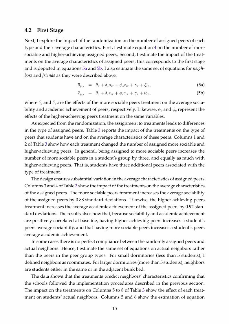
Next, I explore the impact of the randomization on the number of assigned peers of eachtype and their average characteristics. First, I estimate equation 4 on the number of moresociable and higher-achieving assigned peers. Second, I estimate the impact of the treat-ments on the average characteristics of assigned peers; this corresponds to the first stageand is depicted in equations 5a and 5b. I also estimate the same set of equations for neigh-bors and friends as they were described above.

spiτ = θs + δssiτ + φsciτ + γτ + ξiτ , (5a)

cpiτ = θc + δcsiτ + φcciτ + γτ + νiτ , (5b)

where δs and δc are the effects of the more sociable peers treatment on the average socia-bility and academic achievement of peers, respectively. Likewise, φs and φc represent theeffects of the higher-achieving peers treatment on the same variables.

As expected from the randomization, the assignment to treatments leads to differencesin the type of assigned peers. Table 3 reports the impact of the treatments on the type ofpeers that students have and on the average characteristics of these peers. Columns 1 and2 of Table 3 show how each treatment changed the number of assigned more sociable andhigher-achieving peers. In general, being assigned to more sociable peers increases thenumber of more sociable peers in a student’s group by three, and equally as much withhigher-achieving peers. That is, students have three additional peers associated with thetype of treatment.

The design ensures substantial variation in the average characteristics of assigned peers.Columns 3 and 4 of Table 3 show the impact of the treatments on the average characteristicsof the assigned peers. The more sociable peers treatment increases the average sociabilityof the assigned peers by 0.88 standard deviations. Likewise, the higher-achieving peerstreatment increases the average academic achievement of the assigned peers by 0.92 stan-dard deviations. The results also show that, because sociability and academic achievementare positively correlated at baseline, having higher-achieving peers increases a student’speers average sociability, and that having more sociable peers increases a student’s peersaverage academic achievement.

In some cases there is no perfect compliance between the randomly assigned peers andactual neighbors. Hence, I estimate the same set of equations on actual neighbors ratherthan the peers in the peer group types. For small dormitories (less than 5 students), Idefined neighbors as roommates. For larger dormitories (more than 5 students), neighborsare students either in the same or in the adjacent bunk bed.

The data shows that the treatments predict neighbors’ characteristics confirming thatthe schools followed the implementation procedures described in the previous section.The impact on the treatments on Columns 5 to 8 of Table 3 show the effect of each treat-ment on students’ actual neighbors. Columns 5 and 6 show the estimation of equation

15

4 on more sociable and higher-achieving neighbors. Overall, each treatment, more so-ciable and higher-achieving peers, increases the number of neighbors of their respectivetype by 1.6. Columns 7 and 8 show the effect on average neighbors’ characteristics. Be-ing assigned to more sociable peers increases the average sociability of neighbors by 0.557standard deviations. Likewise, the higher-achieving peers treatment increases the aver-age academic achievement of neighbors by 0.59 standard deviations. As expected, dueto the non-compliance reasons mentioned above, these effects are not as large as those incolumns 1 to 4 of Table 3 on assigned peers, but still very strong and highly significant.

4.3 Social Interactions

I now analyze whether students became friends with their neighbors. I show that theintervention had an influence on the social networks in the schools. I do this by showingthat the intervention changed the average characteristics of friends, and it did becausestudents formed new friendhsips with the peers near them in the dormitories.

I use social network data to show how the intervention affected the formation of newfriendships. After the intervention, I administered two surveys with questions that mea-sured social interactions, as shown in the timeline in Figure 1. The first survey took placefour months after the intervention, in August 2017. In this survey, students answeredquestions identifying their friends, study partners, and people with whom they engagedin social activities such as playing games or dancing. The second survey took place in De-cember 2017, using the same set of questions.9 I then constructed a general network thataggregates the answers from both surveys.

To test whether the intervention had an impact on the social network in the schools, Iestimate equation 4 on the number of friends of each type. I also estimate equations 5a and5b on average friends’ characteristics. Columns 9-12 of Table 3 present the results. Beingassigned to more sociable peers increases by 0.483 the number of more sociable friends,and being assigned to higher-achieving peers by 0.414 the number of higher-achievingfriends. These effects translate into an increase of 0.063 and 0.058 standard deviations theaverage sociability and academic achievement of friends, respectively. All of these effectsare statistically significant at the 1% level.

In addition, I also study how the order on the lists affected the social interactionsamong students. I do this by estimating the following equation:

lij = γ0 +9∑

k=1

γk1d=kij + νij. (6)

9In addition to the questions in the first survey, students also answered questions related to collaborationbetween them and diffusion of information in the second round. The questions on cooperation asked fromwhom did they receive help (and who did they help) with their studies and personal problems. Studentsalso named up to five peers who the ministry should contact to diffuse academic or cultural informationduring the vacation period.

16

Equation 6 describes how dummy variables (1d=kij ), denoting the distance between stu-dents i and j on the list change the likelihood of a link (lij) between i and j. The equationincludes nine dummy variables, each of which represents a distance of 1–9 on the list.

The distance between students on the list predicts the formation of social links. PanelA of Figures 3 and 4 shows how the distance on the list predicts the likelihood that two stu-dents will form a social connection out of all the students. Figure 3 shows the estimationof equation 6 by the more sociable treatment status, and Figure 4 by the higher-achievingpeers treatment status. The plots show the estimates of γk with the respective 95% con-fidence interval. Being the neighbor of a student on the list increases the likelihood ofbecoming friends, engaging in social activities together, or studying together by approxi-mately 18 percentage points. Furthermore, there is a decreasing pattern in the distance onthe list, showing that the physical distance in the allocation to dormitories has the powerto predict social interactions.

I find no evidence of heterogeneous effects of distance dummies on social interactionsby the more sociable peers or higher-achieving peers treatments. The plots in Panel A ofFigures 3 and 4 show this clearly since the blue and purple bars—which denote the controland treatment groups, respectively—look very similar.

I also test this formally by estimating whether there are heterogeneous treatment effectsof being neighbors on the list by treatments. Students i and j are neighbors on the listif their names are adjacent, which is equivalent to a distance dij equal to 1. I estimateequation 7, which captures how the likelihood that individuals i and j will have a socialinteraction lij is predicted by being neighbors (neighborij), and neighbors’ heterogeneityby the more sociable treatment, siτ , and the higher-achieving peers treatment, ciτ .

lij = γ0 + γ1neighborij + γ2siτ × neighborij + γ3ciτ × neighborij+∑9

k=2 γk1d=kij + ατ + µijτ ,(7)

The parameters of interest in equation 7 are the impact of being neighbors, γ1, andthe differential effect of being neighbors by the more sociable peers treatment, γ2, and thehigher-achieving peers treatment, γ3.

I find that being neighbors on the list has a substantial effect on the likelihood of form-ing social interactions. The estimates of equation 7 are reported in column 1 of AppendixTable A.5. If two students are neighbors on the list, this increases the likelihood that theywill become friends, study together or engage in social activities together by 16.1 percent-age points (p-value 0.000). I also find that the impact of being neighbors is greater whenthe student is assigned to more sociable peers. In particular, students are 3.7 percentagepoints (p-value 0.014) more likely to form a link with their neighbor when that peer is moresociable. In contrast, I do not find that there is a differentiated effect of being neighborson social interactions when the student is assigned to higher-achieving peers.

For students assessed as less sociable at baseline, distance has the same effect on socialinteractions for those assigned to more and less sociable peers. Panel B of Figure 3 presents

17

the estimates of equation 6 for less sociable students, and Panel C presents the resultsfor more sociable students. Both plots show a similar pattern: distance on the list has adecreasing effect on the likelihood of forming social interactions. Furthermore, for lesssociable students this pattern is similar regardless of whether they are assigned to lesssociable or more sociable peers. By contrast, the plot in Panel C suggests that more sociablestudents are more likely to form social interactions with their neighbors when assigned tomore sociable peers.

I derive the same conclusion by estimating equation 7 by subgroups of sociability atbaseline. Columns 2 and 3 of Table A.5 present the estimation of equation 7 for less andmore sociable students at baseline, respectively. The results are consistent with the discus-sion above. Less sociable students are 16.5 percentage points (p-value 0.000) more likely toform connections with their neighbors. There is no evidence of differentiated impacts ofneighbors in different treatments. By contrast, more sociable students are 14.1 percentagepoints (p-value 0.000) more likely to form connections with their neighbors, 4.8 additionalpercentage points more likely when those neighbors are more sociable (p-value 0.022), and3.5 additional percentage points more likely when those neighbors are higher achieving(p-value 0.106).

Next, I explore differences in the effect of distance by academic achievement at base-line. The evidence suggests that the level of interactions between lower-achieving studentsand higher-achieving peers is similar to the level with lower-achieving peers. Panel B ofFigure 4 presents the estimates of equation 6 for lower-achieving students, and Panel C forhigher-achieving students. Both plots show a decreasing effect of distance on the list onthe likelihood of forming social interactions. For both subgroups, this pattern is similarregardless of being assigned to lower- or higher-achieving peers.

Similar evidence comes from the estimation of equation 7 by academic achievementat baseline. Columns 4 and 5 of Table A.5 present the estimation of equation 7 for lower-and higher-achieving students, respectively. Lower-achieving students are 17 percentagepoints (p-value 0.000) more likely to form connections with their neighbors, and there isno evidence of differentiated impacts of neighbors for either the more sociable or higher-achieving peers treatment. Higher-achieving students are 15.1 percentage points (p-value0.000) more likely to form connections with their neighbors, and 7 additional percentagepoints (p-value 0.001) more likely when those neighbors are more sociable.

The fact that for lower-achieving students there are no differences in social interactionsby peer assignment suggests that there is no sorting by students’ academic achievementin the network formation. This opposed to previous evidence in the literature of peereffects. Carrell et al. (2013) argue that peer effects are negative because lower-achievingstudents interact among themselves, instead of connecting with higher-achieving peers (endogenous social networks). This is not true in my study.

A potential concern with this analysis is that the estimation has assumed link inde-

18

pendence in the network formation. The most recent developments in the econometricsof networks address the correlation between linking decisions.10 In Appendix E, I showthat these results are robust to link dependencies.

In summary, this section concludes that the intervention had an influence on the net-work formation in schools. Students became friends with their peers near them in thedormitories and there is no evidence of of heterogenous effects of proximity on social in-teractions.

5 Outcomes and Empirical Strategy

5.1 Outcomes

In this section I describe the outcomes of my study. These are grouped into two broadcategories according to the type of skill affected: social or cognitive. Social skills outcomesare measured using self-reported instruments and peers’ perception of students accordingto different characteristics. Cognitive skills outcomes are measured by school grades andtest scores collected by the Ministry of Education.

5.1.1 Social Skills Outcomes

The first set of outcomes corresponds to measures of social skills. Finding reliable mea-sures of social skills is a big challenge. I use two categories of social skills outcomes: psy-chological self-reported tests and peers’ perception measures.

My main outcome is expressed as a social skills index. It is constructed using the firstcomponent of a Principal Component Analysis (PCA) on the entire set of tests in this paperthat measure social skills, including peers’ perceptions. The psychological tests used forthis index are described in Appendix C. The peers’ perception measures capture the num-ber of peers who report that the student is in the top five of four school-grade categories:leadership, friendliness, popularity, and shyness.

I reproduce the social skills index, with the available social skills measures at baseline.Appendix Figure A.3 displays a scatterplot between the two measures of students’ socialskills at baseline and after the intervention. There is a large, positive correlation betweenthe two measures. An OLS regression shows that one standard deviation in the socialskills index at baseline is correlated with a 0.43-standard-deviation increase in the socialskills index after the intervention.

The most widely accepted taxonomy of psychological traits, both in the literature andin my data, is the Big Five (McCrae and John, 1992; John and Srivastava, 1999).11 The

10See Chandrasekhar and Jackson (2016), Chandrasekhar (2016), de Paula Aureo et al. (2018), Graham(2017), Mele (2017a), Mele (2017b) for examples.

11Almlund et al. (2011) summarizes the Big Five personality traits and their application to economics.Likewise, Akee et al. (2018); Donato et al. (2017); Kranton and Sanders (2017) provide recent evidence of theBig Five in economics research.

19

American Psychology Association Dictionary defines the Big Five personality traits as follows(Table 1.1 in Almlund et al. (2011)):

1. Conscientiousness: the tendency to be organized, responsible, and hardworking.

2. Openness to Experience: the tendency to be open to new aesthetic, cultural, or intel-lectual experiences.

3. Extraversion: an orientation of one’s interests and energies toward the outer world ofpeople and things rather than the inner world of subjective experience; characterizedby positive affect and sociability.

4. Agreeableness: the tendency to act in a cooperative, unselfish manner.

5. Neuroticism or Emotional Stability: Emotional Stability is “predictability and con-sistency in emotional reactions, with absence of rapid mood changes.” Neuroticismis a chronic level of emotional instability and proneness to psychological distress.

Only two traits from the Big Five are associated with social skills: extraversion12 andagreeableness13. Empirical evidence shows that extraversion is associated with good la-bor market outcomes (Fletcher, 2013), and that agreeableness influences occupational de-cisions (Almlund et al., 2011; Cobb-Clark and Tan, 2011). These results are consistent witha study by Deming (2017) that concludes that the labor market increasingly rewards socialskills.

In addition to the Big Five14, the Ministry of Education collects other self-reported mea-sures of social skills: altruism, empathy, emotional intelligence, intercultural sensitivity,and leadership. As part of the endline survey for this study, we also collected the Readingthe Mind in the Eyes test. Other details for all of these tests are described in Appendix C.

While self-reported psychological tests are frequently used to measure social skills,they are subject to social desirability bias and can be manipulated by the respondent.Since social skills are important for interactions with peers, we also included questionsof how peers perceive students.15 This is additionally supported by empirical evidencewhich shows that relying on the perceptions of members of the same community relaxesinformation asymmetries (Hussam et al., 2017).

Students were asked to rank up to five of their peers in the four dimensions of leader-ship, friendliness, popularity, and shyness. I constructed a measure of peers’ perception

12The facets of extraversion correspond to: warmth (friendly), gregariousness (sociable), assertiveness(self-confident), activity (energetic), excitement seeking (adventurous), and positive emotions (enthusiastic).

13The facets of agreeableness are: trust (forgiving), straight-forwardness (not demanding), altruism(warm), compliance (not stubborn), modesty (not show-off), tender-mindedness (sympathetic).

14The ministry implements the translation of the questionnaire developed by Goldberg (1999) into Spanishfound in Cupani (2009). The English version is available at the following link: https://ipip.ori.org/New_IPIP-50-item-scale.htm. The Spanish version of this test is available upon request.

15This was also the case in the baseline survey, as described in Appendix A.

20

by adding the number of peers who name a given student in each of the four dimensions.The perception measure for individual i corresponds to the number of peers who believethat subject i is in the top five of characteristic c in their school-grade. There is a positivecorrelation between the number of peers who rank the student in the top five on leader-ship, friendliness, and popularity, and a negative correlation with shyness.

5.1.2 Cognitive Outcomes

Teachers assign grades to students for each subject based on their homework and testscores during the first three quarters of the year. Although these variables are available forthe three cohorts, the 2015 cohort reports ony preliminary IB discrete grades with limitedvariation. Since these are only preliminary and there is small variation16 my empiricalanalysis focuses on the grades of the 2016–17 cohorts.

Another reason to focus on these cohorts is that students in the 2016–17 cohorts werealso assessed via standardized tests designed by the Ministry of Education. These testsdetermine the students’ grades for their final quarter at school. For the 2015 cohort, thesetest scores are not available; the Ministry used the IB grades instead.

As described in section 3, the more sociable peers treatment is only available for the2015–16 cohorts. Likewise, test scores and grades are only available for the 2016–17 co-horts. Appendix Table A.10 reconciles both sets of information, and indicates which co-horts were used for each treatment–outcome combination. I still use all the cohorts toestimate the impact of the higher-achieving peers treatment on social skills.

5.2 Empirical Strategy

I begin by estimating the effect of my two treatments—more sociable and higher-achievingpeers—on the social and cognitive skills outcomes described in section 5.1. The followingequation estimates the impact of each treatment:

yiτ = α + λssiτ + λcciτ + γτ + εiτ . (8)

Equation 8 shows how the more sociable peers treatment, siτ , and the higher-achievingpeers treatment, ciτ , affect the outcome, yiτ , of individual i of student type τ . I includestudent type fixed effects, γτ , because the likelihood of receiving the treatments varies bystudent type. The parameters of interest in this equation, λs and λc, the causal impactof the more sociable and higher-achieving peers treatments, respectively. I include thesame set of controls as the ones in the balance tests of section 4. The standard errors areclustered at the student type×group of peer level, since all the students within this unit

16While for the 2016–17 cohorts grades ranged between 1 and 20, for the 2015 cohort students received IBgrades between 1 and 7; 83% of the students in the latter cohort obtained a grade between 3 and 5 for math,and 96% achieved a grade between 4 and 6 for Spanish.

21

share the same treatment peers. I also report the randomization inference p-values for mymain results (Athey and Imbens, 2017; Young, 2017).

Estimates of equation 8 and equations 5a and 5b are of independent interest. Theyalso are the Reduced Form and the First Stage of an IV estimate of the effect of peers’ abil-ities. I estimate the effect of a one-standard-deviation in peers’ average characteristics (i.e.neighbors’ sociability and academic achievement) on students’ outcomes. I use the exper-imental variation in my study in a two-endogenous model, and jointly estimate the effectof peers’ characteristics on the cognitive and social outcomes of students. The followingequation introduces my two-endogenous model:

yiτ = θ + βssniτ + βccniτ + γτ + εiτ , (9)

where sniτ and cniτ denote the average baseline sociability and academic achievement ofstudent i of type τ . For small dormitories (less than 5 students), I define neighbors as peersin the same room. For larger dormitories (more than 5 students), neighbors are definedas having the same or the adjacent bunk bed. The parameters of interest are βs and βc; theeffect of a one standard deviation in the average sociability and academic achievement ofneighbors on students’ outcomes. The first stage of this model is depicted in equations 5aand 5b. It represents the impact of the assignment to treatment on peer characteristics.

As described in section 4, Columns 7 and 8 of Table 3 display the estimates of equations5a and 5b. Being assigned to live with more sociable peers increases the average sociabil-ity of neighbors by 0.55 standard deviations, and the higher-achieving peers treatmentincreases the average academic achievement of neighbors by 0.59 standard deviations.

6 Main Results

This section describes the impact of the intervention on students’ cognitive and social skillsoutcomes. I first present the reduced-form estimates on social skills, then the reduced-form estimates on cognitive skills. Finally, I present the 2SLS estimates using the experi-mental variation as an instrument for neighbors’ sociability and academic achievement atbaseline.

6.1 Social Skills Outcomes

My description of the results starts by reporting the impact of my two treatments—themore sociable peers treatment and the higher-achieving peers treatment—on personalitytraits, peers’ perception, and my social skills index. Panel A of Table 4 reports the reduced-form estimates of equation 8 for all students on all of my social skills indicators.

The results reveal that having more sociable peers has positive effects on openness,extraversion, and agreeableness of the Big Five personality traits. Columns 1 to 5 showthe impact of both treatments on the Big Five: openness, conscientiousness, emotional

22

stability, extraversion, and agreeableness. I focus on the last two traits, which are directlyrelated to social skills. I find that the effect of more sociable peers on extraversion andagreeableness are 0.067 (p-value 0.029) and 0.066 (p-value 0.035) standard deviations, re-spectively. The higher-achieving peers treatment has no effect on the Big Five.

I find no evidence that either the more sociable or the higher-achieving peers treat-ment affects how peers perceive the students. Columns 6 to 9 show the treatment effectson peers’ perception measure for social skills outcomes. The dependent variable in eachcolumn is the number of peers who think a student is in the top five of leadership, friend-liness, popularity, and shyness at the school-by-grade level. Overall, I cannot reject thateither the more sociable peers treatment or the higher-achieving peers treatment do notaffect the peers’ perceptions of a student.

The more sociable peers treatment has a similar positive impact on other measures ofsocial skills and the overall social skills index. Column 10 displays the regression resultsfor an index composed of other measures of social skills, which are described in AppendixC. By contrast, higher-achieving peers do not affect other measures of social skills. Column11 of Table 4 shows the impact of my treatments on my main social skills outcome—thesocial skills index. Overall, the more sociable peers treatment has a positive impact on thesocial skills index. In particular, there is a treatment effect of 0.067 standard deviations (p-value 0.016). Also consistent with my regressions for other social skills outcomes, I cannotrule out the possibility that the higher-achieving peers treatment does not affect the socialskills index.

Table 4 additionally reports the Randomization Inference (RI) p-values of my regres-sions. The null hypothesis for this test is that the outcomes for all units in the samplewould have been the same, regardless of whether the units received the treatment or con-trol status. Thus, the null hypothesis implies that all students would have the same degreeof social skills, regardless of the sociability of their peers. To compute the RI p-values, thetreatments of more sociable peers and higher-achieving peers were randomly reassigned,1,000 times, using the same stratification criteria as the original assignment. I estimateequation 8 for each of these 1,000 permutations. Then I compare the distribution of thecoefficients that were induced by reassignment with the corresponding coefficients, λs andλc , of the real assignment, and produce RI p-values.

The RI p-values are generally consistent with the sampling inference p-values. Overall,I reject the null hypothesis for the more sociable peers treatment on the extraversion andagreeableness traits. I arrive at the same conclusion for my general social skills index incolumn 11. Hence, the results in Panel A of Table 4 suggest that more sociable peers have apositive impact on the formation of students’ social skills. By contrast, there is no evidencethat higher-achieving peers affect cognitive skills.

Next, I explore whether there are heterogeneous treatment effects according to stu-dents’ degree of sociability at baseline. To do this I estimate equation 8 by subgroups: less

23

vs. more sociable students at baseline (Panels B and C, respectively). I then compare theresults for my subgroups to the estimates of equation 8 for all students, presented in PanelA.

The positive effects of the more sociable peers on the social skills of their neighbors aremostly driven by the effect on the less sociable students. Comparing the results in PanelsA and B of Table 4 shows that most of the positive effects of more sociable peers on socialskills are driven by the impact on the students assessed as less sociable at baseline. In par-ticular, more sociable peers have a positive impact on extraversion of 0.084 (p-value 0.067)standard deviations (column 4), and on agreeableness of 0.123 (p-value 0.008) standarddeviations (column 5).

I also find that less sociable students assigned to more sociable peers are perceived tobe more friendly and popular than those who were assigned to less sociable peers. Lesssociable students are perceived to be friendlier by 0.062 (p-value 0.024) standard devia-tions (column 7) and more popular by 0.042 (p-value 0.024) standard deviations (column8). Both effects are statistically significant at the 95% level. These effects amount to anincrease of 0.25 and 0.30, accordingly, in the number of peers who perceive students asfriendly and popular, which represents a respective 13% and 20% increase over the av-erage at baseline. By contrast, higher-achieving peers decrease the number of peers whoperceive the student as friendly and popular.

Likewise, the more sociable peers treatment has a larger effect on other social skills andthe social skills index for less sociable students than for all students. Column 10 showsthat the more sociable peers treatment increases other social skills measures for less so-ciable students by 0.085 standard deviations (p-value 0.029), compared to 0.048 standarddeviations for the average student. The same pattern is observed for the social skills index(column 11)—an increase of 0.114 standard deviations (p-value 0.004) for less sociable stu-dents versus 0.066 standard deviations for average students. Additionally, the RI p-values(all< 0.1) support the general conclusion that more sociable peers have a particularly pos-itive effect on the social skills of less sociable students. The effect of the higher-achievingpeers treatment on both variables is a precise zero.

The more sociable peers treatment does not affect the formation of social skills for stu-dents assessed as more sociable at baseline. Panel C supports this general conclusion byshowing the reverse side of the story. I cannot reject the possibility of zero treatment effectsfor most of the outcomes in this table.

Thus, more sociable peers have a positive impact on the formation of social skills. Theseimpacts are driven by the effects on less sociable students. This reveals how less sociablestudents benefit from being assigned to more sociable peers.

24

6.2 Cognitive Skills Outcomes

Table 5 reports the cognitive skills outcomes based on the estimation of equation 8. Columns1 and 2 report the treatment effects for the grades in math and reading comprehension.Analogously, columns 3 and 4 show the impact of each treatment on math and readingtest scores.

Consistent with the peer effects estimates reported by quasi-experimental studies (An-grist and Lang, 2004; Duflo et al., 2011; Abdulkadiroglu et al., 2014) that generate largevariation in peers’ skills, I find that the impact of higher-achieving peers on students’ aca-demic achievement is a precise zero. Panel A of Table 5 presents the cognitive skills out-comes for all students in my sample. This is a narrowly measured estimate in the context ofmy study. The 95% confidence interval for math test scores ranges between -0.06 and 0.01standard deviations. For reading, it ranges between -0.07 and 0.02 standard deviations.Likewise, I do not find evidence that having more sociable peers affects the formation ofcognitive skills.

Next, I examine treatment effect heterogeneity for the cognitive skills outcomes. I esti-mate equation 8 for two subgroups of academic achievement: lower- and higher-achievingstudents. Panels B and C of Table 5 report the reduced-form estimates for lower- andhigher-achieving students at baseline.

I find that higher-achieving peers have heterogeneous treatment effects on the forma-tion of cognitive skills. Columns 1 and 2 in Panel B of Table 5 show that the higher-achieving peers treatment has a negative effect on grades for both math and reading com-prehension. I first analyze the heterogeneous effects on grades, and find that higher-achieving peers decrease students’ math grades by 0.081 standard deviations (p-value0.019), and reading grades by 0.049 standard deviations (p-value 0.201). I also explorewhether there are heterogeneous effects on test scores. Columns 4 and 5 of Table 5 showthat the effects of higher-achieving peers on lower-achieving students are negative andsignificant for both math (-0.049 with a p-value of 0.054) and reading comprehension (-0.068 with a p-value of 0.045). For the more sociable peers treatment, I arrive at the sameconclusion for both subgroups: I find no evidence that more sociable peers affect the for-mation of cognitive skills. The heterogeneous effects that I find for both grades and testscores are consistent with the RI p-values.

Finally, I show that the effects of higher-achieving peers are indeed statistically differ-ent for higher- and lower- achieving students at baseline.

In summary, higher-achieving peers have, on average a zero effect on students’ over-all cognitive outcomes, but they are detrimental to the academic achievement of lower-achieving students.

25

6.3 2SLS Estimates

Table 6 presents the results of the 2SLS two-endogenous model described by equation 9on social and cognitive skills. These estimates are useful to provide magnitudes that arecomparable with other peer effects studies. The table reports the estimates of parametersβs and βc, the impact of neighbors’ average sociability and academic achievement on stu-dents’ outcomes. There are two endogenous variables: neighbors’ sociability and neigh-bors’ academic achievement (both calculated at baseline). I instrument for these variablesusing indicators for whether the student was assigned to the more sociable or the higher-achieving peers treatment. The table shows the estimation for five dependent variables:social skills index (column 1), math grades (column 2), reading comprehension grades(column 3), math test scores (column 4), and reading test scores (column 5).

I find that neighbors’ sociability has a positive impact on social skills, but no impact oncognitive outcomes. Panel A of Table 6 shows the results for all students. A one-standard-deviation increase in neighbors’ sociability has a 0.132-standard-deviation impact (p-value0.009) on the social skills index for the average student (column 1). I cannot reject an effectequal to zero on grades or test scores (columns 2-5).

Nor can I reject that the academic achievement of neighbors at baseline has a zero im-pact on social and cognitive skills outcomes. The 95% confidence interval of a one standarddeviation in neighbors’ baseline academic achievement ranges between -0.11 and 0.02 formath test scores (Table 6 Panel A, column 4), and between -0.12 and 0.03 for reading testscores (Table 6 Panel A, column 5). This rules out both the positive peer effects estimates ofexploiting random allocation to dorms (between 0.06 and 0.12 standard deviations), andthe large peer effects estimates of exploiting random allocation to large groups such asclassrooms or squadrons (0.35-0.53 standard deviations).

The positive impact of neighbors’ sociability on social skills is driven by the effect onstudents assessed as less sociable at baseline. I explore heterogeneity in baseline sociabilityby reporting the estimates of equation 9 for less sociable students in Panel B of Table 6 andthe estimates for more sociable students in Panel C. Consistent with the results in Table 4, aone-standard-deviation increase in neighbors’ average sociability at baseline increases thesocial skills index for less sociable students by 0.237 standard deviations (p-value 0.002).By contrast, the impact on more sociable students has a small point estimate, 0.031 , and itis not possible to reject that it is equal to zero (p-value 0.632). The estimates also show thatfor less sociable students, higher-achieving peers have a negative impact on math grades(Table 6 Panel B, column 2, p-value: 0.098) and more sociable peers have a negative impacton math test scores (Table 6 Panel B, column 4, p-value: 0.045). However, these effects arenot consistent across the other outcomes. In a similar fashion, more sociable peers havea positive impact on reading comprehension grades for more sociable students (p-value0.094).

26

The results also show that neighbors’ sociability has a positive impact on lower-achievingstudents’ social skills. Panels D and E of Table 6 show the estimation of equation 9 byacademic achievement at baseline. Panel D reports the estimates of βs and βc for lower-achieving students, and Panel E for higher-achieving students. A one-standard-deviationincrease in neighbors’ sociability produces a 0.254-standard-deviation increase in the so-cial skills index for lower-achieving students (p-value 0.001).

By contrast, there is suggestive evidence that neighbors’ academic achievement hasa negative impact on test scores for lower-achieving students. A one standard deviationin neighbors’ academic achievement at baseline decreases math grades by 0.150 (p-value0.018), reading grades by 0.093 (p-value 0.219), math test scores by 0.082 (p-value 0.082),and reading test scores by 0.122 standard deviations (p-value 0.040) for lower-achievingstudents. For higher-achieving students, there is no evidence that either neighbors’ socia-bility or academic achievement affects social or cognitive skills outcomes.

In summary, the conclusions of the 2SLS model are the same as those using the reduced-form estimates, and the estimates are precise enough to rule out even small effects ofhigh-achieving peers on cognitive skills. Having more sociable neighbors has a positiveimpact on social skills for less sociable students. Likewise, the evidence suggests that hav-ing higher-achieving neighbors has a detrimental effect on the academic achievement oflower-achieving students.

7 Mechanism: Self-Confidence

Next, I explore potential mechanisms that might explain my results.Recall that peer effects were negative for lower-achieving students. According to Car-

rell et al. (2013), peer effects are negative because lower-achieving students interact amongstthemselves, instead of connecting with higher-achieving peers (endogenous social net-works). I test this hypothesis as a mechanism that can explain the results in my study andexplore other potential mechanisms that might describe my findings. Whatever mecha-nism is operating in the backend of my intervention, it must be able to explain two mainoutcomes from my study:

1. More sociable peers have a positive effect on the formation of social skills, particu-larly for less sociable students.

2. Higher-achieving peers have a negative effect on academic achievement for lower-achieving students, and no effect on average.

Moving back to subsection 5.1.1, I reviewed how the intervention impacted the net-work formation and the social interactions that students develop. However, some of theevidence presented there also rules out that the number of social interactions between stu-dents and their peers explains my findings. More precisely, I find no evidence that less

27

sociable students have more interactions with more —rather than less— sociable peers,or that lower-achieving students are interacting or studying less with higher-achievingpeers. The evidence indicating that lower-achieving students befriend higher-achievingpeers and still have lower academic achievement contradicts the hypothesis introducedby Carrell et al. (2013). In my study, even though lower-achieving students interact withhigher-achieving peers, they still experience declines in academic achievement.

In this section, I study whether changes in the self-confidence of students in their skillscan explain my results. The main idea behind this mechanism is that students updatetheir beliefs about their social and cognitive skills by interacting with their peers. First,I address the self-confidence story through the lens of the confidence-enhanced perfor-mance model from Compte and Postlewaite (2004). I show that my empirical findings areconsistent with students: (1) succeeding in social activities with peers when at least oneof them is sociable, and (2) failing in cognitive activities when they perform worse thantheir peers. Furthermore, I provide empirical evidence suggesting that the interventionchanged students’ self-confidence in their skills.

7.1 Theoretical Framework7.1.1 General Model

The model that I describe next is based on Compte and Postlewaite (2004). The modeladdresses how peer effects can shift students’ beliefs about their skills—defined as self-confidence— and eventually change students’ outcomes. I extend the model to two activ-ities: (1) activities with neighbors (type n) and (2) other activities (type (o). By changingthe probability of success in activities type n, students change their level of confidencewhich affects their general outcomes and investment decisions.17 All proofs are providedin Appendix D.

In the model, the agent faces a sequence of decisions for each time period t whethershe decides or not to invest in an activity. There are two types of activities: n and o. Under-taking an activity entails a cost c. This cost is stochastic with support in [0, 1]. The randomvariables {ct}∞t=1 are independent, and when the agent makes a decision at t, she knowsthe realization of ct and the type of the activity n or o.

In this theoretical framework, success in both types of activities depends on the self-confidence of the agent, and her self-confidence depends on her perception of past suc-cesses. Let ρa denote the probability of success in an activity of type a, for a = {n, o}, andκ ∈ (0, 1] as a measure of the agent’s self-confidence. The model assumes that:

ρa = κµa,

17The model in Compte and Postlewaite (2004) focuses on how biases in information processing can en-hance welfare. Here, I don’t introduce any bias in the recall of failures. Instead, I focus on how changes inthe probability of success in activities with peers can affect the general success of the student.

28

where µa is an exogenous parameter—the probability of success in an activity of type a,that does not depend on the agent’s self-confidence.

The level of self-confidence κ is a function of the empirical frequency of past successesφ in activities n and o:

κ = κ(φ),

φ = γφn + (1− γ)φo,

where φa = sasa+fa

is the frequency of success in activities of type a, sa denotes the numberof successes and fa the number of failures. The parameter γ is the weight the agent assignsto the n activities in her past successes. I will assume that γ ∈ (0, 1), so that the agentdecides on both types of activities.

The model assumes that κ is a smooth and increasing function of φ: κ = κ(φ), whereκ′(·) > 0, κ(0) > 0, and, without loss of generality κ(1) = 1. Combining the two functionsabove, the probability of success in an activity is a function of the perception of success φ,where:

ρa(φ) = κ(φ)µa, for a = {n, o}.

Finally, the model assumes that the effect of self-confidence on performance cannot be toostrong, that is, ρ′a(φ) < 1.18

An equilibrium in this model implies that for each type of activity, the probability ofsuccess coincides with the agent’s perception of the frequency of success. Among thepossible perceptions φ that an agent may have about the frequency of success, the onethat plays a focal role is the unique perception φ∗, such that:

φ∗n = κ(φ∗)µn, (10a)

φ∗o = κ(φ∗)µo, (10b)

where φ∗ = γφ∗n + (1− γ)φ∗o.The agent assesses whether it is worth investing in an activity of type a and forms a

belief pa on whether or not she will succeed. With a belief pat about her chance of successat time t, the agent compares the expected payoff from undertaking the activity to its cost.The agent only undertakes the activity a if and only if:

pat ≥ ct.

The belief of success is a function of the data that she recollects: pa = β(sa, fa). Thisfunction can be interpreted as an agent who is initially unsure of the probability of successin activities a and updates her initial beliefs as she acumulates experience. The restrictionson the function β are the following:

(i) ∀s, f ≥ 0, 0 < β(sa, fa) < 1.18This assumption guarantees an interior solution for the level of self-confidence in equilibrium.

29

(ii) There exists A > 0 such that ∀sa, fa > 0, |β(sa, fa)− sa(sa + fa)| ≤ Asa+fa

.

The first assumption states that beliefs must lie between 0 and 1. The second assump-tion is for “asymptotic consistency”, ruling out belief formation processes for which thereis a permanent divergence between the agent’s perceived successes and failures and herbeliefs.

Compte and Postlewaite (2004) show that under these conditions, beliefs are correct inthe long run, and lim

t→∞pat = ρa(φ

∗). The agent invests in an activity in the long-run whenρa(φ

∗) ≥ ct, and this probability is given by:

Pr(ct ≤ ρa(φ∗)) =

∫ ρa(φ∗)

0

g(c)dc = G(ρa(φ∗)),

where G(·) corresponds to the c.d.f. of the cost parameter c. I assume that G(·) has no flatregions.

To understand the impact of the intervention on students’ self-confidence and theirsubsequent changes in skills, I will argue that the intervention changed the parameter µn:the probability of success that doesn’t depend on the self-confidence of the individual inactivitiesn. This parameter affects students’ self-confidence and the likelihood of investingin activities n through two different channels: (1) a direct channel, whereby the agentexogenously becomes more likely to succeed, and (2) an indirect channel, whereby shegains self-confidence in her skills and this translates into a larger probability of success inequilibrium. Hence, through self-confidence, an increase in µn amplifies the probabilityof success for the agent in activities n. We can observe these effects by calculating thederivative of equation 10a with respect to µn:

dφ∗ndµn

= κ(·)︸︷︷︸direct channel

+ κ′(·)µndφ∗

dµn︸ ︷︷ ︸indirect channel

(11)

Equation 11 reveals the the two channels through which changes in µn can affect theprobability of success in equilibrium φ∗n: the direct channel is given by changes in µn, andthe indirect channel—where I choose to focus my attention—is determined by the increasein self-confidence κ′(·) of an individual in equilibrium. Both channels jointly explain howincreasing the parameter µn leads to an agent’s higher success in activities r in equlibrium.

The changes in µn also affect the probability of success in other activities through self-confidence. More specifically, they affect the probability of success of the second type ofactivity in this model, activities of type o. We can observe this by applying the implicitfuntion theorem to 10b:

dφ∗odµn

= µo κ′(·)dφ∗

dµn︸ ︷︷ ︸self-confidence

(12)

The overall changes in the probability of success in both types of activities, accountingfor the fact that dφ∗

dµnis also determined in equilibrium, is summarized as follows:

30

Proposition 1. Under the assumptions that κ′(·) > 0, κ(0) > 0, ρ′a(φ) < 1, and γ ∈ (0, 1),then:

1. The probability of success in activities n in equilibrium φ∗n increases with µn.

2. The probability of success in activities o in equilibrium φ∗o increases with µn.

3. The level of self-confidence in equilibrium κ(φ∗) increases with µn.

Corollary 1. The probability that the agent invests in both types of activities in equilibrium is anincreasing function of the parameter µn.

Once the agent becomes more likely to succeed, she is willing to invest more frequentlyin equilibrium. There is a direct channel for activities n, and an indirect channel throughwhich self-confidence influences an individual’s success, both in activities of type n ando.

7.1.2 The Intervention

To understand this model in the context of my intervention, I will assume that activities ninvolve interactions with neighbors, and activities o do not. The randomization changedthe peer characteristics and hence generated variation in the parameter µn. In particular, astudent’s success in neighbor activities depends on the characteristics of the student andher neighbors. More precisely, the parameter µn is determined by the types of the studentand her neighbor. I consider only two types of individuals i ∈ {l, h} and assume that:

µn = µn(τi, τj) for τi, τj = {h, l}.

where τi and τj are the types of individual i (the student) and j (the student’s neighbor),respectively.

Furthermore, I consider two types of activities: social and cognitive activities.

(a) Social activities form social skills. These are described as activities where studentsinteract with peers by having a conversation or playing a game. Neighbor activitiesinvolve interaction with neighbors and other activities involve interaction with otherpeople. Success in a social activity can be intuitively described by a student who en-joyed the interaction.

(b) Cognitive activities form cognitive skills. Cognitive activities involve the likes of study-ing for a test, attending class or receiving support from a tutor. Success can take differ-ent shapes for neighbor and other activities. For example, success in other activitiescan occur when a student learns or when she receives a good grade. Alternatively,success in neighbor activities is defined as a situation where students do not performworse than their neighbors. That is, I will assume that students will have a lower utilityif they underperfom or learn less than their neighbors: cognitive success in neighboractivities is determined relatively, not absolutely.

31

I impose two additional assumptions on the likelihood of a student’s success. Theprobability of success in neighbor activities depends on student and neighbor types asfollows:

Assumption 1. Social success: The probability of success in a social neighbor activity is largerwhen either the student or her neighbor is high in social skills: µn(l, l) < µn(·, h) = µn(h, ·).

Under this assumption, a student is prone to feel good about participating in social activ-ities with their neighbors when at least one of them is more sociable.

Assumption 2. Cognitive success: The probability of success in a cognitive neighbor activ-ity is lower when the student is a low-type and her neighbor a high-type: µn(l, h) < µn(l, l) =µn(h, h) = µn(l, h).

Under this assumption, students care about their relative ranking and avoid doing worsethan their peers. A student is more likely perform worse than her neighbor when she islower-achieving and her neighbor is higher-achieving.

Proposition 2. Under the assumption of social success:

1) When assigned to more sociable peers, in equilibrium less sociable students:

(a) Invest more in social activities with neighbors.(b) Invest more in other social activities.(c) Increase their self-confidence in social skills.

2) More sociable students do not change their self-confidence or investment decisions onsocial skills.

The intuition behind this statement is that less sociable students benefit from interact-ing with more sociable peers. It is a direct result of proposition 1. Less-sociable studentscan more easily engage in conversations or other activities with more sociable—ratherthan less sociable—neighbors. As a result, students feel more successful in social activ-ities. The higher the success, the more the increase in students’ self-confidence, whichloops back into more successful activities with neighbors as well as with other people. Bycontrast, the intervention did not change the probability of success of more sociable stu-dents in social neighbor activities. Hence, the sociability of neighbors does not affect theself-confidence of more sociable students. This rationalizes why more sociable studentsdo not change their social skills under the lens of this model.

Proposition 3. Under the assumption of cognitive success:

1) When assigned to higher-achieving peers, in equilibrium lower-achieving students:

(a) Invest less in cognitive activities with neighbors.(b) Invest less in other cognitive activities.(c) Decrease their self-confidence in cognitive skills.

32

2) Higher-achieving students do not change their self-confidence or investment decisionson cognitive skills.

The intuition behind this statement is that lower-achieving students feel less accom-plished when they compare their performance to their higher-achieving neighbros. Thelower the perceived success, the greater the frustration, and the lower the self-confidence,which brings down their investment in cognitive skills. The lower self-confidence loopsback into less successful study interactions with their neighbors as well as other learn-ing activities. By contrast, the intervention did not change the probability of success forhigher-achieving students in cognitive neighbor activities. Hence, higher-achieving stu-dents did not experience changes in their academic achievement.

Why changes in self-confidence asymmetrically affect the formation of social and cog-nitive skills? The measurement of cognitive and social skills could potentially explain thisdifference. While schools regularly test academic performance and students can visiblybe ranked based on it, there is no such clearly defined measure of social skills. Most mea-sures of social skills are not only based on self-perception, but more importantly, studentsdo not have information on the individual versus peer contribution to the formation ofsocial skills. Hence, when they perceive a high level of social skills due to the interactionwith sociable peers, students are likely to believe that their individual contribution is high,reinforcing the idea that they are successful in social activities.

7.2 Empirical Evidence

In this section I present empirical evidence suggesting that self-confidence is a mechanismdriving my results.

First, I study whether less sociable students feel they have better social interactionswhen assigned to more sociable peers. Through the lens of the model of the previous sec-tion, this can be interpreted as having more success in social activities. Table 7 presentsthese results on the following set of variables: whether the student feels supported by herfriends (column 1), the level of satisfaction with her dormitory (column 2), whether thestudent thinks she is friends with her neighbors (column 3), whether the student reportsbeing empathetic to her neighbors (column 4), whether the student reports that her neigh-bors are empathetic to her (column 5)19, whether the student reports that their neighborsare worried for her problems (column 6), and a neighbors’ quality index that aggregatesall these variables (column 7).

There is evidence suggesting that less sociable students perceive a higher quality ofinteractions with neighbors when assigned to more sociable peers. Panels A and B of Ta-ble 7 present the results on social interactions quality for less sociable and more sociable

19Only a random sample of the students answered the two questions of empathy in the social networksurvey in August 2017.

33

students, respectively. The results show that less sociable students perceive a higher qual-ity of social interactions when assigned to more sociable peers. They feel more supportedby their friends, a higher level of satisfaction with their dormitory, and that their neigh-bors are more empathetic to them. The results in column 6 show that the more sociablepeers treatment has an impact of 0.345 standard deviations (p-value 0.010) on the qualityindex for less sociable students. By contrast, while more sociable students report a higherquality of interactions (Panel B, column 7), this difference is not statistically significant.

Second, I find evidence that less sociable students changed their beliefs about their so-cial skills due to the intervention. To support this claim, I estimate equation 8 based onwhether the student named herself (weighted by the ranking) in the top five of leader-ship, friendliness, popularity, and shyness in her school-by-grade. Table 8 presents theseresults. Panels A and B show the results for students assessed as less sociable and moresociable at baseline. The estimates in Panel A show that except for leadership (column1), the student is more likely to consider herself friendly (column 2), popular (column 3),and not shy (column 4) if she is assigned to more sociable peers. While some of theseimpacts are not significant, the effect on an index constructed by aggregating these threevariables (column 5) is statistically significant at the 95% level. Including leadership inthe index (column 6) reduces the size of the impact. However, it is still large in magni-tude compared to the effects on the self-confidence of the more sociable students (Panel Bof Table 8). This evidence suggests that the intervention increased less sociable students’self-confidence in their level of social skills. I also find no such effect for the more sociablestudents which is consistent with the assumptions of the model described before.

I also estimate whether lower-achieving students changed their beliefs about their cog-nitive skills due to the higher-achieving peers treatment. The estimates of equation 8 foroutcomes of self-confidence in cognitive skills are presented in Table 9. Panel A shows theresults for the lower-achieving students, and Panel B for the higher-achieving students.The set of outcomes in the table are:

• Belonging to the school (column 1): in the endline survey students indicated thedegree to which they felt they belonged to the school (0 to 100).

• Academic ranking: students estimated their academic ranking in the school (column2) and relative to their friends (column 3).

• Goals relative to peers: students answered the Achievement Goal Questionnaire.20 Twoof the factors of the test involve the student comparing herself to her peers: whetherthe student wants to perform well compared to other students (column 4), and whetherthe student avoids doing worse than other students (column 5).

20The details of the test are discussed in Appendix C.

34

• Academically skilled: whether the student considers herself one of the top five mostacademically skilled in the school, weighted by the ranking (column 6).

• Volunteering to receive information about scholarship and other academic opportu-nities, and the ranking the student gave herself for receiving this information (col-umn 7).

• A self-confidence index that aggregates all the variables in columns 1 to 7.

My results show that lower-achieving students had lower levels of self-confidence intheir cognitive skills when assigned to higher-achieving peers. The treatment effects ofhigher-achieving peers on the variables of self-confidence for lower-achieving studentsare presented in Panel A of Table 9. In column 1, I find that lower-achieving students de-crease their belief that they belong to the school by 0.06 standard deviations (p-value 0.086)when assigned to higher-achieving peers. Since the COAR Network is designed for high-achieving students, the changes in beliefs are consistent with students feeling that theyunderachieve and are not part of the academic community because of it. Columns 2 and3 show that these students also report having a lower academic ranking in the school andrelative to their friends, although only the latter is statistically different from zero. Like-wise, they are less likely to report that they want to perform better (column 4) or avoiddoing worse than their peers (column 5). They are also less likely to name themselvesamong the top five most-skilled students (column 6), and to volunteer to receive informa-tion about scholarships and other academic opportunities (column 7). These results are allsummarized by the effect on the self-confidence index in column 8; the higher-achievingpeers treatment has a negative effect on self-confidence for lower-achieving students of0.301 standard deviations (p-value 0.007). In comparison to the results in Panel B, the esti-mates for the higher-achieving students in Panel C do not suggest that peer characteristicschanged their beliefs about their skills.

Thus, my empirical evidence suggests that by interacting with more sociable peers, lesssociable students gained self-confidence in their social skills. Similarly, by interacting withhigher-achieving, lower-achieving students lost self-confidence in their cognitive skills,which can explain why they have a lower academic performance.

In summary, this section provided a simple theoretical framework and empirical evi-dence that suggests that the type of peer had an impact on the students’ self-confidence.Hence, I cannot rule out self-confidence as a mechanism driving my results on social andcognitive skills.

8 Conclusion

While there is a positive return to social skills in the labor market, there is still little ev-idence on how social skills form. This paper presents the results of a field experiment

35

designed to estimate causal cognitive and social peer effects. The study was conductedin 23 out of 25 exam schools in Peru, covering a sample of approximately 6,000 students.Students were classified by baseline sociability and academic achievement using central-ity measures of social networks and test scores. Unlike previous experimental designs,I have shown that it is possible to guarantee strong variation in peer characteristics byrandomizing the type of peer and matching students to peers of their treatment groups.

I found that more sociable peers have a positive impact on the development of socialskills. These effects are mainly driven by the impact on those who were assessed as lesssociable at baseline. My results show that they became more extroverted and showed ahigher level of agreeableness, the two components of the Big Five personality traits relatedto social skills. These effects are robust to other psychological tests that measure socialskills and to measures that account for self-reported biases. Less sociable students withmore sociable peers were perceived to be more friendly and popular in their school.

By contrast, I do reject positive cognitive peer effects on the formation of cognitiveskills. For students who were lower achieving at baseline, the evidence suggests that thehigher-achieving peers treatment has a negative effect. My rejection of positive cognitivepeer effects is consistent with the evidence from quasi-experimental studies (Angrist andLang, 2004; Abdulkadiroglu et al., 2014; Rao, 2013). The findings contradict the positivepeer effects of studies that use random allocation to groups (Sacerdote, 2011; Epple andRomano, 2011), highlighting the methodological concerns associated with this type of de-sign, as pointed out by Angrist (2014).

I have shown that my results are consistent with the idea that students changed theirself-confidence by interacting with their assigned peers. I presented a simple theoreticalframework through which I can reproduce the empirical primary findings under reason-able assumptions for the model. The main intuition behind the model is that studentsdo not know their level of skills but update their beliefs after interacting with their peers.Hence, students changed their investment decisions due to the updated beliefs about theirsuccess in social and cognitive activities. Furthermore, there is empirical evidence sug-gesting that self-confidence explains my results on the formation of social skills and aca-demic achievement.

I also study the role of social interactions as a mechanism of how peer characteristicsaffect the formation of skills. I can rule out the level of interactions as a mechanism. Whilethe intervention had a substantial impact on social network formation in the schools, I donot find that less sociable students interact more with more sociable peers.

Similarly, although lower-achieving students are befriending and studying with higher-achieving peers, they experience a decline in academic achievement. This result contra-dicts previous evidence in the literature which suggests students only benefit from higher-achieving peers when they are interacting with them (Carrell et al., 2013).

In conclusion, while the existing literature and education policies have focused on

36

peers’ academic achievement, this paper shows that in the setting of selective boardingschools in Peru, the role of sociable peers is more important. Further studies are neededto assess whether these results are valid in other contexts and the impact of these effectson labor market outcomes.

References

Abdulkadiroglu, A., Angrist, J., and Pathak, P. (2014). The elite illusion: Achievementeffects at boston and new york exam schools. Econometrica, 82(1):137–196.

Adhvaryu, A., Kala, N., and Nyshadham, A. (2018). The skills to pay the bills: Returnsto on-the-job soft skills training. Working Paper 24313, National Bureau of EconomicResearch.

Akee, R., Copeland, W., Costello, E. J., and Simeonova, E. (2018). How does house-hold income affect child personality traits and behaviors? American Economic Review,108(3):775–827.

Almlund, M., Duckworth, A. L., Heckman, J., and Kautz, T. (2011). Chapter 1 - person-ality psychology and economics1. In Hanushek, E. A., Machin, S., and Woessmann, L.,editors, Handbook of The Economics of Education, volume 4 of Handbook of the Economics ofEducation, pages 1 – 181. Elsevier.

Andrews, I., Sotck, J., and Sun, L. (2018). Weak instruments in iv regression: Theory andpractice.

Angrist, J. D. (2014). The perils of peer effects. Labour Economics, 30:98 – 108. SpecialSection articles on.

Angrist, J. D. and Lang, K. (2004). Does school integration generate peer effects? evidencefrom boston’s metco program. American Economic Review, 94(5):1613–1634.

Arli, S. K. and Bakan, A. B. (2018). An investigation of the relationship between intercul-tural sensitivity and compassion in nurses. International Journal of Intercultural Relations,63:38 – 42.

Athey, S. and Imbens, G. (2017). Chapter 3 - the econometrics of randomized experimentsa.In Banerjee, A. V. and Duflo, E., editors, Handbook of Field Experiments, volume 1 of Hand-book of Economic Field Experiments, pages 73 – 140. North-Holland.

Autor, D. (2014). Polanyi’s paradox and the shape of employment growth. Working Paper20485, National Bureau of Economic Research.

37

Banerjee, A., Chandrasekhar, A. G., Duflo, E., and Jackson, M. O. (2013). The diffusion ofmicrofinance. Science, 341(6144).

Banerjee, A., Chandrasekhar, A. G., Duflo, E., and Jackson, M. O. (2014). Gossip: Identi-fying central individuals in a social network. Working Paper 20422, National Bureau ofEconomic Research.

Beaman, L. and Dillon, A. (2018). Diffusion of agricultural information within social net-works: Evidence on gender inequalities from mali. Journal of Development Economics,133:147 – 161.

Belloni, A., Chernozhukov, V., and Hansen, C. (2014a). High-dimensional methods andinference on structural and treatment effects. Journal of Economic Perspectives, 28(2):29–50.

Belloni, A., Chernozhukov, V., and Hansen, C. (2014b). Inference on treatment effects afterselection among high-dimensional controls†. The Review of Economic Studies, 81(2):608–650.

Boisjoly, J., Duncan, G. J., Kremer, M., Levy, D. M., and Eccles, J. (2006). Empathy orantipathy? the impact of diversity. American Economic Review, 96(5):1890–1905.

Breza, E. and Chandrasekhar, A. (2018). Social networks, reputation, and commitment:Evidence from a savings monitors field experiment. Technical report.

Bursztyn, L., Egorov, G., and Jensen, R. (2018). Cool to be smart or smart to be cool?understanding peer pressure in education. The Review of Economic Studies, page rdy026.

Caeyers, B. and Fafchamps, M. (2016). Exclusion bias in the estimation of peer effects.Working Paper 22565, National Bureau of Economic Research.

Carre, A., Stefaniak, N., D’Ambrosio, F., Bensalah, L., and Besche, C. (2013). The basicempathy scale in adults (bes-a): Factor structure of a revised form. 25:679–691.

Carrell, S., Fullerton, R. L., and West, J. (2009). Does your cohort matter? measuring peereffects in college achievement. Journal of Labor Economics, 27(3):439–464.

Carrell, S. E., Sacerdote, B. I., and West, J. E. (2013). From natural variation to optimalpolicy? the importance of endogenous peer group formation. Econometrica, 81(3):855–882.

Castro-Solano, A. (2007). Teorıa y Evaluacion dell Liderazgo. Paidos.

Chandrasekhar, A. (2016). The Oxford Handbook of the Economics of Networks, chapter Econo-metrics of Network Formation. Oxford Handbook Series.

38

Chandrasekhar, A. and Jackson, M. O. (2016). A Network Formation Model Based onSubgraphs. ArXiv e-prints.

Chen, G.-M. and Starosta, W. J. (2000). The development and validation of the interculturalsensitivity scale. Human Communication.

Cobb-Clark, D. A. and Tan, M. (2011). Noncognitive skills, occupational attainment, andrelative wages. Labour Economics, 18(1):1 – 13.

Colman, A. M. (2009). A Dictionary of Psychology.

Compte, O. and Postlewaite, A. (2004). Confidence-enhanced performance. American Eco-nomic Review, 94(5):1536–1557.

Cupani, M. (2009). El cuestionario de personalidad ipip-ffm: Resultados preliminares deuna adaptacion en una muestra de preadolescentes argentinos. 6:51–58.

de Paula Aureo, Seth, R.-S., and Elie, T. (2018). Identifying preferences in networks withbounded degree. Econometrica, 86(1):263–288.

Declerck, C. H. and Bogaert, S. (2008). Social value orientation: related to empathy andthe ability to read the mind in the eyes. The Journal of social psychology, 148.

Deming, D. J. (2017). The growing importance of social skills in the labor market. QuarterlyJournal of Economics, 132(4):1593–1640.

Donato, K., Miller, G., Mohanan, M., Truskinovsky, Y., and Vera-Hernandez, M. (2017).Personality traits and performance contracts: Evidence from a field experiment amongmaternity care providers in india. American Economic Review, 107(5):506–10.

Duflo, E., Dupas, P., and Kremer, M. (2011). Peer effects, teacher incentives, and the im-pact of tracking: Evidence from a randomized evaluation in kenya. American EconomicReview, 101(5):1739–74.

Epple, D. and Romano, R. E. (2011). Chapter 20 - peer effects in education: A survey ofthe theory and evidence. volume 1 of Handbook of Social Economics, pages 1053 – 1163.North-Holland.

Fabregas, R. (2017). A better school but a worse position? the effects of marginal schooladmissions in mexico city. Technical report, Harvard University. Job Market Paper.

Falk, A., Kosse, F., Deckers, T., Pinger, P., and Schildberg-Horisch, H. (2018). The formationof prosociality: Causal evidence on the role of social environment. Technical report,University of Bonn.

39

Fletcher, J. M. (2013). The effects of personality traits on adult labor market outcomes:Evidence from siblings. Journal of Economic Behavior & Organization, 89:122 – 135.

Fryer, R. and Austen-Smith, D. (2005). An economic analysis of ’acting white’. QuarterlyJournal of Economics.

Gambin, M. and Sharp, C. (2018). The relations between empathy, guilt, shame and de-pression in inpatient adolescents. Journal of Affective Disorders, 241:381 – 387.

Garlick, R. (2018). Academic peer effects with different group assignment policies: Res-idential tracking versus random assignment. American Economic Journal: Applied Eco-nomics, 10(3):345–69.

Goldberg, L. R. (1999). Personality Psychology in Europe, volume 7, chapter A broad-bandwidth, public domain, personality inventory measuring the lower-level facets ofseveral five-factor models. Tilburg University Press.

Golsteyn, B., Non, A., and Zolitz, U. (2017). The impact of peer personality on academicachievement. Technical report, University of Zurich.

Gordon, S. R. and Mwavita, M. (2018). Evaluating the international dimension in an un-dergraduate curriculum by assessing students’ intercultural sensitivity. Studies in Edu-cational Evaluation, 59:76 – 83.

Graham, B. S. (2017). An econometric model of network formation with degree hetero-geneity. Econometrica, 85(4):1033–1063.

Handcock, M. S., Hunter, D. R., Butts, C. T., Goodreau, S. M., Krivitsky, P. N., and Morris,M. (2018). ERGM: Fit, Simulate and Diagnose Exponential-Family Models for Networks.

Handcock, M. S., Hunter, D. R., Butts, C. T., Goodreau, S. M., Krivitsky, P. N., Morris, M.,and de Moll, S. B. (2016). Exponential random graph models (ergms) using statnet.

Hussam, R., Rigol, N., and Roth, B. (2017). Targeting high ability entrepreneurs usingcommunity information. Technical report, MIT M.

J. Elliot, A. and Murayama, K. (2008). On the measurement of achievement goals: Critique,illustration, and application. 100.

John, O. P. and Srivastava, S. (1999). Handbook of Personality: Theory and Research, chapterThe Big Five trait taxonomy: History, measurement, and theoretical perspectives, pages102–138. Guilford Press, New York, second edition.

Jolliffe, D. and Farrington, D. P. (2006). Development and validation of the basic empathyscale. Journal of Adolescence, 29(4):589 – 611.

40

Kranton, R. E. and Sanders, S. G. (2017). Groupy versus non-groupy social preferences:Personality, region, and political party. American Economic Review, 107(5):65–69.

Lavy, V. and Sand, E. (2012). The friends factor: How students’ social networks affecttheir academic achievement and well-being? Working Paper 18430, National Bureau ofEconomic Research.

Law, K., Wong, C.-S., and J Song, L. (2004). The construct and criterion related validity ofemotional intelligence and its potential utility for management studies. 89:483–96.

Manski, C. F. (1993). Identification of endogenous social effects: The reflection problem.The Review of Economic Studies, 60(3):pp. 531–542.

Marsh, H. W. and Parker, J. W. (1984). Determinants of student self-concept: Is it better tobe a relatively large fish in a small pond even if you don’t learn to swim as well? Journalof Personality and Social Psychology, 47(1):213–231.

McCrae, R. R. and John, O. P. (1992). An introduction to the five-factor model and itsapplications. Journal of Personality, 60(2):175–215.

Mehu, M., Grammer, K., and Dunbar, R. I. (2007). Smiles when sharing. Evolution andHuman Behavior, 28(6):415 – 422.

Mele, A. (2017a). A structural model of dense network formation. Econometrica, 85(3):825–850.

Mele, A. (2017b). A structural model of homophily and clustering in social networks.Technical report, Johns Hopkins University.

Otto, P. E. and Bolle, F. (2011). Multiple facets of altruism and their influence on blooddonation. The Journal of Socio-Economics, 40(5):558 – 563.

Pop-Eleches, C. and Urquiola, M. (2013). Going to a better school: Effects and behavioralresponses. American Economic Review, 103(4):1289–1324.

Rao, G. (2013). Familiarity does not breed contempt: Diversity, discrimination and gen-erosity in delhi schools. Technical report, Department of Economics, Berkeley Univer-sity.

Ribas, R., Sampaio, B., and Trevisan, G. (2018). Can better peers signal less success? thedisruptive effect of perceived rank on career investment. Technical report.

Rushton, J. P., Chrisjohn, R. D., and Fekken, G. C. (1981). The altruistic personality andthe self-report altruism scale. Personality and Individual Differences, 2(4):293 – 302.

41

Sacerdote, B. (2001). Peer effects with random assignment: Results for dartmouth room-mates. The Quarterly Journal of Economics, 116(2):681–704.

Sacerdote, B. (2011). Chapter 4 - peer effects in education: How might they work, how bigare they and how much do we know thus far? volume 3 of Handbook of the Economics ofEducation, pages 249 – 277. Elsevier.

Villadangos, M., Errasti, J., Amigo, I., Jollife, D., and Garcıa-Cueto, E. (2016). Charac-teristics of empathy in young people measured by the spanish validation of the basicempathy scale. Psicothema.

Wai, M. and Tiliopoulos, N. (2012). The affective and cognitive empathic nature of thedark triad of personality. Personality and Individual Differences, 52(7):794 – 799.

Weinberger, C. J. (2014). The increasing complementarity between cognitive and socialskills. The Review of Economics and Statistics, 96(5):849–861.

Woolley, A. W., Chabris, C. F., Pentland, A., Hashmi, N., and Malone, T. W. (2010). Evi-dence for a collective intelligence factor in the performance of human groups. Science,330(6004):686–688.

Young, A. (2017). Channelling fisher: Randomization tests and the statistical insignifi-cance of seemingly significant experimental results. Technical report, London School ofEconomics.

Yukl, G. (2013). Leadership in Organizations. Pearson, eighth edition edition.

42

Table 1: Summary Statistics at Baseline

All Students By Sociability By Academic AchievementLess Sociable More Sociable Lower Achieving Higher Achieving

Variable (1) (2) (3) (4) (5)Sociability (centrality measure) -0.00 -0.64 0.64 -0.04 0.04

(1.00) (0.51) (0.96) (0.99) (1.01)Academic achievement (score in the admission test) 0.00 -0.08 0.08 -0.79 0.78

(0.99) (0.96) (1.02) (0.47) (0.71)Poor (%) 0.36 0.39 0.35 0.39 0.33Extremely poor (%) 0.18 0.22 0.18 0.21 0.16Rural (%) 0.26 0.31 0.23 0.30 0.22

N 6,147 1,832 1,822 3,069 3,078

Notes: This table reports summary statistics by type of student. Column 1 shows statistics for all students, and columns 2 to 5 ac-cording to the classification of students by social and cognitive skills. To classify students as more vs. less sociable, I use sociability atbaseline as measured by the eigenvector centrality of an aggregate social network of dorm preferences, friendships, study, and socialpartnerships. Eigenvector centrality measures a student’s influence student in the network. A student with a high eigenvector scoreis connected to other students who themselves have a high influence as well. Eigenvector centrality is not measured for the 2017 co-hort. To classify students as higher vs. lower achieving, I use the score in the admissions test to the COAR Network, which evaluatesthe applicants in math and reading comprehension. For sociability and admissions test scores at baseline, standard deviations arereported in parentheses. The table includes a set of three demographic characteristics of students, including poverty, extreme poverty,and whether the student comes from a rural household. These demographic variables come from government administrative data.

43

Table 2: Balance on Cognitive and Social Skills at Baseline

Social Skills Index Math Score Reading ScoreAll students Sociability All students Academic Achievement All students Academic Achievement

Variable Less Sociable More Sociable Lower Achieving Higher Achieving Lower Achieving Higher Achieving(1) (2) (3) (4) (5) (6) (7) (8) (9)

More sociable peers -0.041 -0.033 -0.050 0.019 0.019 0.019 0.010 0.022 -0.002(0.082) (0.117) (0.111) (0.027) (0.034) (0.042) (0.028) (0.040) (0.040)

Higher-achieving peers 0.048 0.130 0.003 0.016 -0.023 0.053 -0.000 -0.012 0.011(0.059) (0.116) (0.110) (0.023) (0.030) (0.034) (0.023) (0.032) (0.033)

Control mean -0.05 -0.39 0.26 -0.11 -0.39 0.31 -0.08 -0.31 0.25More sociable F p-value 0.89 0.57 0.91 0.89 0.82 0.92 0.89 0.82 0.92Higher-achieving F p-value 0.73 0.77 0.49 0.73 0.80 0.40 0.73 0.80 0.40N 6,103 1,832 1,822 4,553 2,274 2,279 4,553 2,274 2,279

Notes: This table reports balance checks of being assigned to more sociable and higher-achieving peers on social and cognitive skills outcomes for all students and subgroups by sociability and academicachievement at baseline. All regressions include strata fixed effects and control for the baseline value of the dependent variable. For the 2017 cohort all regressions include strata-by-classroom fixedeffects. To classify students as more vs. less sociable, I use sociability at baseline as measured by the eigenvector centrality of an aggregate social network of dorm preferences, friendships, study, andsocial partnerships. Eigenvector centrality measures a student’s influence in the network. A student with a high eigenvector score is connected to other students who themselves have a high influenceas well. Eigenvector centrality is not measured for the 2017 cohort. To classify students as higher vs. lower achieving, I use the score in the admissions test to the COAR Network, which evaluates theapplicants in math and reading comprehension. The control group is defined as being assigned to less sociable and lower-achieving peers. The “More sociable F p-value” and the “Higher-achieving Fp-value” correspond to the F-statistic of the respective treatment of multivariate regressions that include all variables at baseline presented in Appendix Tables A.3 and A.4. Standard errors are clusteredat the peer group type-by-type level; *** p-value<0.01, ** p-value<0.05, * p-value<0.1.

44

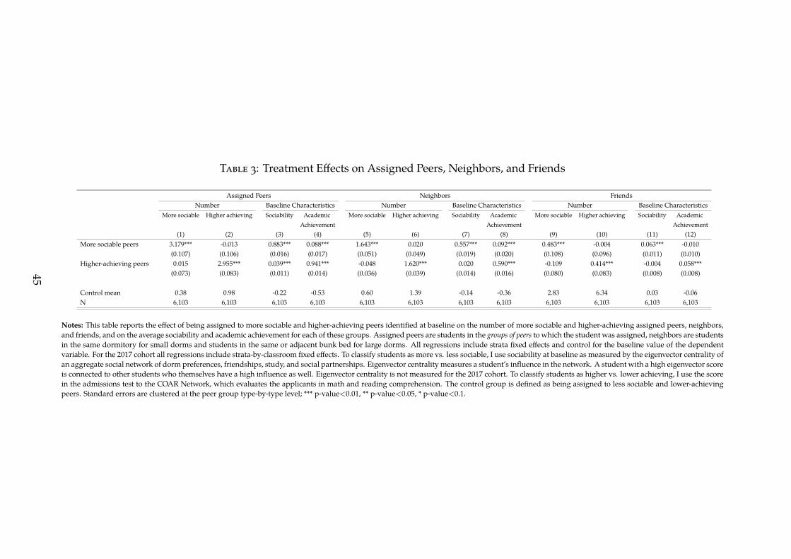
Table 3: Treatment Effects on Assigned Peers, Neighbors, and Friends

Assigned Peers Neighbors FriendsNumber Baseline Characteristics Number Baseline Characteristics Number Baseline Characteristics

More sociable Higher achieving Sociability Academic More sociable Higher achieving Sociability Academic More sociable Higher achieving Sociability AcademicAchievement Achievement Achievement

(1) (2) (3) (4) (5) (6) (7) (8) (9) (10) (11) (12)More sociable peers 3.179*** -0.013 0.883*** 0.088*** 1.643*** 0.020 0.557*** 0.092*** 0.483*** -0.004 0.063*** -0.010

(0.107) (0.106) (0.016) (0.017) (0.051) (0.049) (0.019) (0.020) (0.108) (0.096) (0.011) (0.010)Higher-achieving peers 0.015 2.955*** 0.039*** 0.941*** -0.048 1.620*** 0.020 0.590*** -0.109 0.414*** -0.004 0.058***

(0.073) (0.083) (0.011) (0.014) (0.036) (0.039) (0.014) (0.016) (0.080) (0.083) (0.008) (0.008)

Control mean 0.38 0.98 -0.22 -0.53 0.60 1.39 -0.14 -0.36 2.83 6.34 0.03 -0.06N 6,103 6,103 6,103 6,103 6,103 6,103 6,103 6,103 6,103 6,103 6,103 6,103

Notes: This table reports the effect of being assigned to more sociable and higher-achieving peers identified at baseline on the number of more sociable and higher-achieving assigned peers, neighbors,and friends, and on the average sociability and academic achievement for each of these groups. Assigned peers are students in the groups of peers to which the student was assigned, neighbors are studentsin the same dormitory for small dorms and students in the same or adjacent bunk bed for large dorms. All regressions include strata fixed effects and control for the baseline value of the dependentvariable. For the 2017 cohort all regressions include strata-by-classroom fixed effects. To classify students as more vs. less sociable, I use sociability at baseline as measured by the eigenvector centrality ofan aggregate social network of dorm preferences, friendships, study, and social partnerships. Eigenvector centrality measures a student’s influence in the network. A student with a high eigenvector scoreis connected to other students who themselves have a high influence as well. Eigenvector centrality is not measured for the 2017 cohort. To classify students as higher vs. lower achieving, I use the scorein the admissions test to the COAR Network, which evaluates the applicants in math and reading comprehension. The control group is defined as being assigned to less sociable and lower-achievingpeers. Standard errors are clustered at the peer group type-by-type level; *** p-value<0.01, ** p-value<0.05, * p-value<0.1.

45

Table 4: Reduced-Form Estimates on Social Skills

Big Five Personality Traits Peers’ Perceptions Other Measures Social SkillsOpenness Conscientiousness Emotional Extraversion Agreeableness Leadership Friendliness Popularity Shyness of social skills Index

Stability

(1) (2) (3) (4) (5) (6) (7) (8) (9) (10) (11)Panel A: All Students

More sociable peers 0.066** 0.026 0.035 0.067** 0.066** 0.002 0.037 0.026 0.009 0.048* 0.067**(0.032) (0.032) (0.031) (0.031) (0.031) (0.019) (0.024) (0.019) (0.017) (0.028) (0.027)

Higher-achieving peers 0.024 0.031 0.025 -0.006 -0.007 0.050*** -0.023 0.008 -0.016 -0.008 -0.006(0.026) (0.026) (0.026) (0.026) (0.026) (0.019) (0.024) (0.020) (0.017) (0.023) (0.022)

RI p-value more sociable peers 0.036 0.464 0.298 0.048 0.066 0.944 0.148 0.268 0.674 0.156 0.030RI p-value higher-achieving peers 0.340 0.252 0.342 0.856 0.854 0.028 0.326 0.820 0.444 0.856 0.878

Control mean -0.05 0.01 0.01 -0.03 -0.02 -0.05 -0.02 -0.04 0.02 -0.01 -0.01N 4,942 4,942 4,942 4,942 4,942 3,544 3,544 3,544 3,544 6,103 6,103

Panel B: Less Sociable Students at BaselineMore sociable peers 0.080* 0.023 0.060 0.084* 0.123*** 0.004 0.061** 0.049** 0.013 0.085** 0.114***

(0.045) (0.046) (0.042) (0.045) (0.046) (0.021) (0.027) (0.022) (0.029) (0.039) (0.039)Higher-achieving peers -0.039 0.047 0.051 -0.056 0.024 -0.012 -0.094*** -0.060*** -0.022 0.016 0.008

(0.043) (0.044) (0.041) (0.044) (0.045) (0.022) (0.028) (0.023) (0.030) (0.038) (0.038)

RI p-value more sociable peers 0.092 0.642 0.204 0.078 0.018 0.910 0.046 0.050 0.712 0.074 0.004RI p-value higher-achieving peers 0.386 0.342 0.324 0.264 0.654 0.600 0.002 0.010 0.476 0.724 0.856

Control mean -0.15 -0.17 -0.16 -0.16 -0.24 -0.24 -0.31 -0.19 0.17 -0.21 -0.26N 1,536 1,536 1,536 1,536 1,536 1,763 1,763 1,763 1,763 1,832 1,832

Panel C: More Sociable Students at BaselineMore sociable peers 0.053 0.028 0.010 0.051 0.012 0.003 0.023 0.004 0.005 0.010 0.019

(0.042) (0.042) (0.045) (0.039) (0.041) (0.032) (0.039) (0.031) (0.019) (0.039) (0.037)Higher-achieving peers 0.083** 0.021 0.020 0.006 -0.033 0.108*** 0.053 0.075** -0.009 -0.012 -0.011

(0.041) (0.042) (0.045) (0.039) (0.041) (0.030) (0.037) (0.031) (0.019) (0.039) (0.037)

RI p-value more sociable peers 0.240 0.560 0.848 0.280 0.858 0.954 0.588 0.996 0.788 0.802 0.630RI p-value higher-achieving peers 0.070 0.688 0.678 0.946 0.460 0.002 0.244 0.046 0.718 0.718 0.754

Control mean -0.03 -0.09 -0.04 0.04 -0.02 0.10 0.24 0.06 -0.18 -0.01 0.01N 1,570 1,570 1,570 1,570 1,570 1,781 1,781 1,781 1,781 1,822 1,822

p-value of difference 0.655 0.941 0.416 0.594 0.072 0.903 0.498 0.263 0.816 0.175 0.079

Notes: This table reports the effect of being assigned to more sociable and higher-achieving peers identified at baseline based on personality traits, peers’ perceptions, and social skills outcomes. All regressions include strata fixed effects andcontrol for the baseline value of the dependent variable. For the 2017 cohort all regressions include strata-by-classroom fixed effects. To classify students as more vs. less sociable, I use sociability at baseline as measured by the eigenvectorcentrality of an aggregate social network of dorm preferences, friendships, study, and social partnerships. Eigenvector centrality measures a student’s influence in the network. A student with a high eigenvector score is connected to otherstudents who themselves have a high influence as well. Eigenvector centrality is not measured for the 2017 cohort. To classify students as higher vs. lower achieving, I use the score in the admissions test to the COAR Network, which evaluatesthe applicants in math and reading comprehension. The control group is defined as being assigned to less sociable and lower-achieving peers. Personality traits correspond to the Big Five. Measures of peers’ perceptions correspond tothe number of peers who think the student is in the top five of leadership, friendliness, popularity, and shyness (school-by-grade). The table presents two social skills indexes for robustness. The first is constructed using PCA on all thevariables that measure social skills (see Appendix C for details), excluding personality traits and measures of peers’ perceptions. The second index is constructed using PCA on all the variables that measure social skills (see Appendix C fordetails). The table also reports the RI p-values of each treatment. The treatments were randomly reassigned on 1,000 permutations of students. Each outcome variable was then regressed on the reassigned treatment indicators. The truecoefficients were then compared to the distribution of coefficients induced by reassignment in order to generate the RI p-values. The last row reports the p-value of equal treatment effects of more sociable peers for less sociable and moresociable students at baseline. Standard errors are clustered at the peer group type-by-type level; *** p-value<0.01, ** p-value<0.05, * p-value<0.1.

46

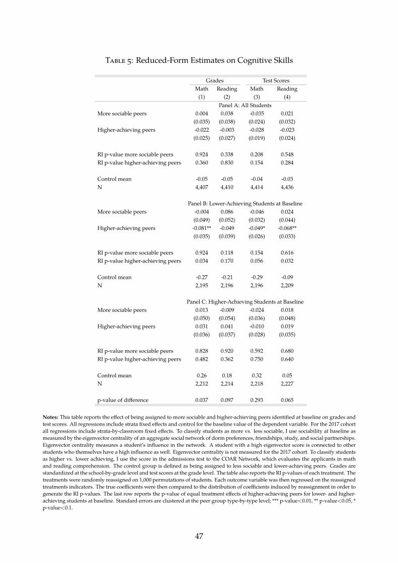
Table 5: Reduced-Form Estimates on Cognitive Skills

Grades Test ScoresMath Reading Math Reading

(1) (2) (3) (4)Panel A: All Students

More sociable peers 0.004 0.038 -0.035 0.021(0.035) (0.038) (0.024) (0.032)

Higher-achieving peers -0.022 -0.003 -0.028 -0.023(0.025) (0.027) (0.019) (0.024)

RI p-value more sociable peers 0.924 0.338 0.208 0.548RI p-value higher-achieving peers 0.360 0.830 0.154 0.284

Control mean -0.05 -0.05 -0.04 -0.03N 4,407 4,410 4,414 4,436

Panel B: Lower-Achieving Students at BaselineMore sociable peers -0.004 0.086 -0.046 0.024

(0.049) (0.052) (0.032) (0.044)Higher-achieving peers -0.081** -0.049 -0.049* -0.068**

(0.035) (0.039) (0.026) (0.033)

RI p-value more sociable peers 0.924 0.118 0.154 0.616RI p-value higher-achieving peers 0.034 0.170 0.056 0.032

Control mean -0.27 -0.21 -0.29 -0.09N 2,195 2,196 2,196 2,209

Panel C: Higher-Achieving Students at BaselineMore sociable peers 0.013 -0.009 -0.024 0.018

(0.050) (0.054) (0.036) (0.048)Higher-achieving peers 0.031 0.041 -0.010 0.019

(0.036) (0.037) (0.028) (0.035)

RI p-value more sociable peers 0.828 0.920 0.592 0.680RI p-value higher-achieving peers 0.482 0.362 0.750 0.640

Control mean 0.26 0.18 0.32 0.05N 2,212 2,214 2,218 2,227

p-value of difference 0.037 0.097 0.293 0.065

Notes: This table reports the effect of being assigned to more sociable and higher-achieving peers identified at baseline on grades andtest scores. All regressions include strata fixed effects and control for the baseline value of the dependent variable. For the 2017 cohortall regressions include strata-by-classroom fixed effects. To classify students as more vs. less sociable, I use sociability at baseline asmeasured by the eigenvector centrality of an aggregate social network of dorm preferences, friendships, study, and social partnerships.Eigenvector centrality measures a student’s influence in the network. A student with a high eigenvector score is connected to otherstudents who themselves have a high influence as well. Eigenvector centrality is not measured for the 2017 cohort. To classify studentsas higher vs. lower achieving, I use the score in the admissions test to the COAR Network, which evaluates the applicants in mathand reading comprehension. The control group is defined as being assigned to less sociable and lower-achieving peers. Grades arestandardized at the school-by-grade level and test scores at the grade level. The table also reports the RI p-values of each treatment. Thetreatments were randomly reassigned on 1,000 permutations of students. Each outcome variable was then regressed on the reassignedtreatments indicators. The true coefficients were then compared to the distribution of coefficients induced by reassignment in order togenerate the RI p-values. The last row reports the p-value of equal treatment effects of higher-achieving peers for lower- and higher-achieving students at baseline. Standard errors are clustered at the peer group type-by-type level; *** p-value<0.01, ** p-value<0.05, *p-value<0.1.

47

Table 6: 2SLS Estimates of Social and Cognitive Peer Effects on Students’ Outcomes

Social Skills Index Grades Test ScoresMath Reading Math Reading

(1) (2) (3) (4) (5)Panel A: All Students

Roommates’ sociability 0.132*** 0.010 0.068 -0.052 0.061(0.050) (0.064) (0.070) (0.044) (0.057)

Roommates’ academic achievement -0.021 -0.059 -0.015 -0.045 -0.047(0.038) (0.044) (0.047) (0.033) (0.041)

N 5,988 4,343 4,346 4,350 4,372

Panel B: Less Sociable Students at BaselineRoommates’ sociability 0.237*** -0.001 -0.037 -0.129** 0.057

(0.075) (0.097) (0.108) (0.064) (0.090)Roommates’ academic achievement -0.017 -0.135* 0.049 -0.057 -0.104

(0.063) (0.077) (0.087) (0.053) (0.074)

N 1,793 993 994 995 1,008

Panel C: More Sociable Students at BaselineRoommates’ sociability 0.031 0.016 0.152* -0.010 0.067

(0.064) (0.084) (0.090) (0.059) (0.070)Roommates’ academic achievement -0.016 -0.042 -0.048 0.030 -0.036

(0.061) (0.084) (0.088) (0.062) (0.067)

N 1,782 1,015 1,014 1,014 1,021

Panel D: Lower-Achieving Students at BaselineRoommates’ sociability 0.254*** 0.015 0.153* -0.065 0.062

(0.068) (0.087) (0.093) (0.056) (0.074)Roommates’ academic achievement -0.051 -0.150** -0.091 -0.082* -0.122**

(0.058) (0.064) (0.071) (0.047) (0.058)

N 2,999 2,169 2,170 2,171 2,184

Panel E: Higher-Achieving Students at BaselineRoommates’ sociability 0.011 0.013 -0.022 -0.031 0.065

(0.075) (0.096) (0.104) (0.069) (0.089)Roommates’ academic achievement 0.004 0.015 0.053 -0.020 0.017

(0.052) (0.060) (0.061) (0.047) (0.056)

N 2,989 2,174 2,176 2,179 2,188

Notes: This table reports 2SLS estimates of neighbors’ average sociability and academic achievement at baseline on students’ out-comes. There are two endogenous variables: neighbors’ sociability and neighbors’ academic achievement at baseline. I instrumentfor these using indicators for whether the student was assigned to the more sociable or higher-achieving peers treatment. Neighborsare students in the same dormitory for small dormitories and students in the same or adjacent bunk bed for large dormitories. Allregressions include strata fixed effects and control for the baseline value of the dependent variable. For the 2017 cohort all regressionsinclude strata-by-classroom fixed effects. To classify students as more vs. less sociable, I use sociability at baseline as measured bythe eigenvector centrality of an aggregate social network of dorm preferences, friendships, study, and social partnerships. Eigenvec-tor centrality measures a student’s influence in the network. A student with a high eigenvector score is connected to other studentswho themselves have a high influence as well. Eigenvector centrality is not measured for the 2017 cohort. To classify students ashigher vs. lower achieving, I use the score in the admissions test to the COAR Network, which evaluates the applicants in math andreading comprehension. The control group is defined as being assigned to less sociable and lower-achieving peers. The social skillsindex is constructed using PCA on all the variables that measure social skills (see Appendix C for details). Grades are standardizedat the school-by-grade level and test scores at the grade level. Standard errors are clustered at the peer group type-by-type level; ***p-value<0.01, ** p-value<0.05, * p-value<0.1.

48

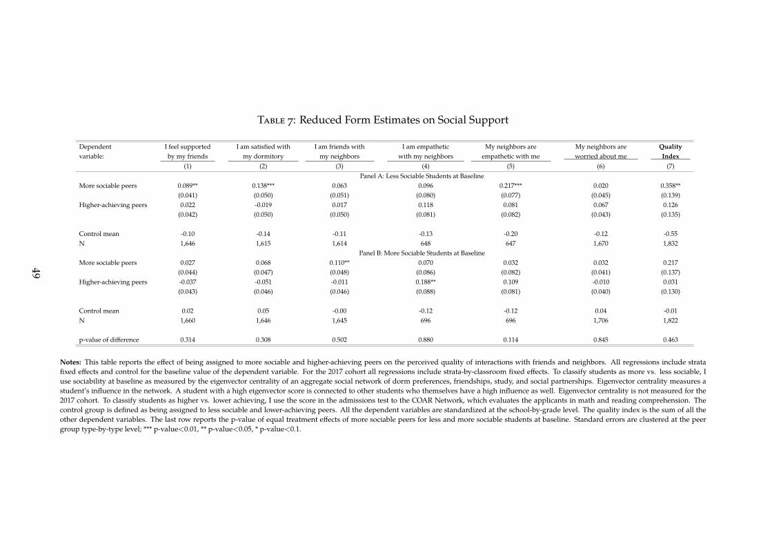
Table 7: Reduced Form Estimates on Social Support

Dependent I feel supported I am satisfied with I am friends with I am empathetic My neighbors are My neighbors are Qualityvariable: by my friends my dormitory my neighbors with my neighbors empathetic with me worried about me Index

(1) (2) (3) (4) (5) (6) (7)Panel A: Less Sociable Students at Baseline

More sociable peers 0.089** 0.138*** 0.063 0.096 0.217*** 0.020 0.358**(0.041) (0.050) (0.051) (0.080) (0.077) (0.045) (0.139)

Higher-achieving peers 0.022 -0.019 0.017 0.118 0.081 0.067 0.126(0.042) (0.050) (0.050) (0.081) (0.082) (0.043) (0.135)

Control mean -0.10 -0.14 -0.11 -0.13 -0.20 -0.12 -0.55N 1,646 1,615 1,614 648 647 1,670 1,832

Panel B: More Sociable Students at BaselineMore sociable peers 0.027 0.068 0.110** 0.070 0.032 0.032 0.217

(0.044) (0.047) (0.048) (0.086) (0.082) (0.041) (0.137)Higher-achieving peers -0.037 -0.051 -0.011 0.188** 0.109 -0.010 0.031

(0.043) (0.046) (0.046) (0.088) (0.081) (0.040) (0.130)

Control mean 0.02 0.05 -0.00 -0.12 -0.12 0.04 -0.01N 1,660 1,646 1,645 696 696 1,706 1,822

p-value of difference 0.314 0.308 0.502 0.880 0.114 0.845 0.463

Notes: This table reports the effect of being assigned to more sociable and higher-achieving peers on the perceived quality of interactions with friends and neighbors. All regressions include stratafixed effects and control for the baseline value of the dependent variable. For the 2017 cohort all regressions include strata-by-classroom fixed effects. To classify students as more vs. less sociable, Iuse sociability at baseline as measured by the eigenvector centrality of an aggregate social network of dorm preferences, friendships, study, and social partnerships. Eigenvector centrality measures astudent’s influence in the network. A student with a high eigenvector score is connected to other students who themselves have a high influence as well. Eigenvector centrality is not measured for the2017 cohort. To classify students as higher vs. lower achieving, I use the score in the admissions test to the COAR Network, which evaluates the applicants in math and reading comprehension. Thecontrol group is defined as being assigned to less sociable and lower-achieving peers. All the dependent variables are standardized at the school-by-grade level. The quality index is the sum of all theother dependent variables. The last row reports the p-value of equal treatment effects of more sociable peers for less and more sociable students at baseline. Standard errors are clustered at the peergroup type-by-type level; *** p-value<0.01, ** p-value<0.05, * p-value<0.1.

49

Table 8: Reduced-Form Estimates on Self-Confidence in Social Skills

Dependent Self-perception Self-confidence Indexvariable: I am in the top five of: Excluding All variables

Leadership Friendliness Popularity Shyness leadership(1) (2) (3) (4) (5) (6)

Panel A: Less Sociable Students at BaselineMore sociable peers -0.044 0.037 0.061 0.072* 0.169** 0.129

(0.042) (0.045) (0.045) (0.043) (0.078) (0.097)Higher-achieving peers -0.003 -0.043 0.003 -0.020 -0.061 -0.066

(0.043) (0.045) (0.044) (0.043) (0.076) (0.094)

Control mean -0.05 -0.01 -0.01 -0.06 -0.07 -0.12N 1,681 1,681 1,681 1,681 1,832 1,832

Panel B: More Sociable Students at BaselineMore sociable peers -0.087* -0.025 0.001 -0.003 -0.040 -0.128

(0.045) (0.047) (0.045) (0.040) (0.080) (0.101)Higher-achieving peers 0.053 -0.016 -0.071 0.040 -0.048 -0.001

(0.046) (0.048) (0.045) (0.039) (0.077) (0.101)

Control mean 0.02 -0.00 0.00 -0.02 -0.02 -0.00N 1,710 1,710 1,710 1,710 1,822 1,822

p-value of difference 0.474 0.339 0.337 0.203 0.062 0.069

Notes: This table reports the effect of being assigned to more sociable and higher-achieving peers identified on self-confidence in socialskills. All regressions include strata fixed effects and control for the baseline value of the dependent variable. For the 2017 cohortall regressions include strata-by-classroom fixed effects. To classify students as more vs. less sociable, I use sociability at baseline asmeasured by the eigenvector centrality of an aggregate social network of dorm preferences, friendships, study, and social partnerships.Eigenvector centrality measures a student’s influence in the network. A student with a high eigenvector score is connected to otherstudents who themselves have a high influence as well. Eigenvector centrality is not measured for the 2017 cohort. To classify studentsas higher vs. lower achieving, I use the score in the admissions test to the COAR Network, which evaluates the applicants in math andreading comprehension. The control group is defined as being assigned to less sociable and lower-achieving peers. All the dependentvariables are standardized at the school-by-grade level, and weighted by the ranking that the student assigned to herself in the survey.In column 5, the self-confidence index is the sum of all the other dependent variables excluding leadership. In column 6, the self-confidence index is the sum of all the other dependent variables. The last row reports the p-value of equal treatment effects of moresociable peers for less and more sociable students at baseline. Standard errors are clustered at the peer group type-by-type level; ***p-value<0.01, ** p-value<0.05, * p-value<0.1.

50

Table 9: Reduced-Form Estimates of Self-Confidence in Cognitive Skills

Dependent What is my level What is my academic ranking: Goals with respect to peers: Self-perception: Self-confidencevariable: of belonging in the school? among friends? I try to I avoid I am in the top five of I volunteer to receive Index

to the school perform better doing worse academically skilled academic information(1) (2) (3) (4) (5) (6) (7) (8)

Panel A: Lower-Achieving Students at BaselineMore sociable peers -0.003 -0.037 -0.037 -0.015 0.008 -0.028 0.012 -0.118

(0.041) (0.042) (0.044) (0.048) (0.048) (0.037) (0.042) (0.123)Higher-achieving peers -0.066* -0.035 -0.089** -0.068* -0.032 -0.017 -0.072** -0.318***

(0.035) (0.035) (0.036) (0.041) (0.041) (0.033) (0.035) (0.106)

Control mean 0.02 -0.08 -0.05 0.03 -0.04 -0.07 0.02 0.35N 2,801 2,813 2,805 2,680 2,680 2,829 2,829 3,050

Panel B: Higher-Achieving Students at BaselineMore sociable peers 0.009 -0.019 0.027 -0.079 -0.050 -0.085* 0.007 -0.107

(0.043) (0.042) (0.043) (0.048) (0.044) (0.050) (0.045) (0.133)Higher-achieving peers 0.044 0.004 -0.023 -0.006 0.002 0.065 0.033 0.109

(0.035) (0.033) (0.035) (0.038) (0.036) (0.040) (0.037) (0.108)

Control mean -0.02 0.11 0.09 0.00 0.06 0.08 -0.01 0.72N 2,856 2,855 2,854 2,763 2,763 2,867 2,867 3,053

p-value of difference 0.027 0.429 0.191 0.270 0.537 0.118 0.041 0.005

Notes: This table reports the effect of being assigned to more sociable and higher-achieving peers on self-confidence in cognitive skills. All regressions include strata fixed effects and control for thebaseline value of the dependent variable. For the 2017 cohort all regressions include strata-by-classroom fixed effects. To classify students as more vs. less sociable, I use sociability at baseline as measuredby the eigenvector centrality of an aggregate social network of dorm preferences, friendships, study, and social partnerships. Eigenvector centrality measures a student’s influence in the network. Astudent with a high eigenvector score is connected to other students who themselves have a high influence as well. Eigenvector centrality is not measured for the 2017 cohort. To classify students as highervs. lower achieving, I use the score in the admissions test to the COAR Network, which evaluates the applicants in math and reading comprehension. The control group is defined as being assigned toless sociable and lower-achieving peers. All the dependent variables are standardized at the school-by-grade level. The self-perception measures are weighted by the ranking that the student assignedto herself in the survey. The self-confidence index is the sum of all the other dependent variables. The last row reports the p-value of equal treatment effects of higher-achieving peers for lower andhigher-achieving students at baseline. Standard errors are clustered at the peer group type-by-type level; *** p-value<0.01, ** p-value<0.05, * p-value<0.1.

51

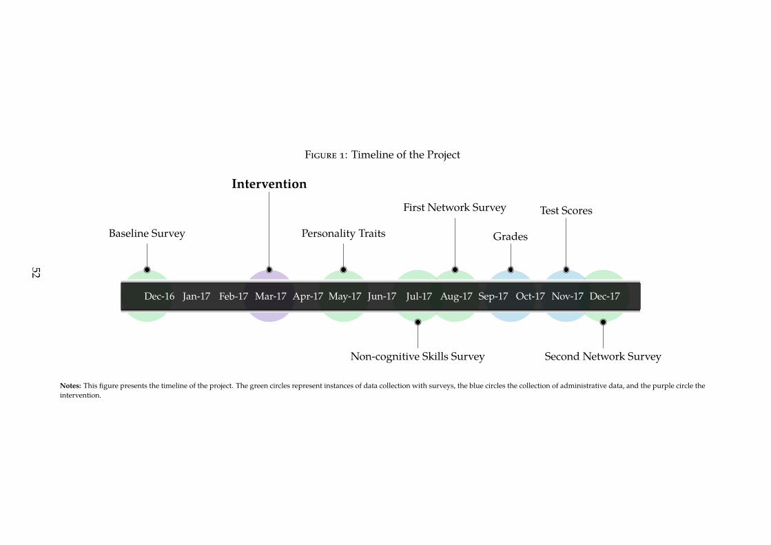
Figure 1: Timeline of the Project

Dec-16 Jan-17 Feb-17 Mar-17 Apr-17 May-17 Jun-17 Jul-17 Aug-17 Sep-17 Oct-17 Nov-17 Dec-17

Baseline Survey

Intervention

Personality Traits

Non-cognitive Skills Survey

First Network Survey

Grades

Test Scores

Second Network Survey

Notes: This figure presents the timeline of the project. The green circles represent instances of data collection with surveys, the blue circles the collection of administrative data, and the purple circle theintervention.

52

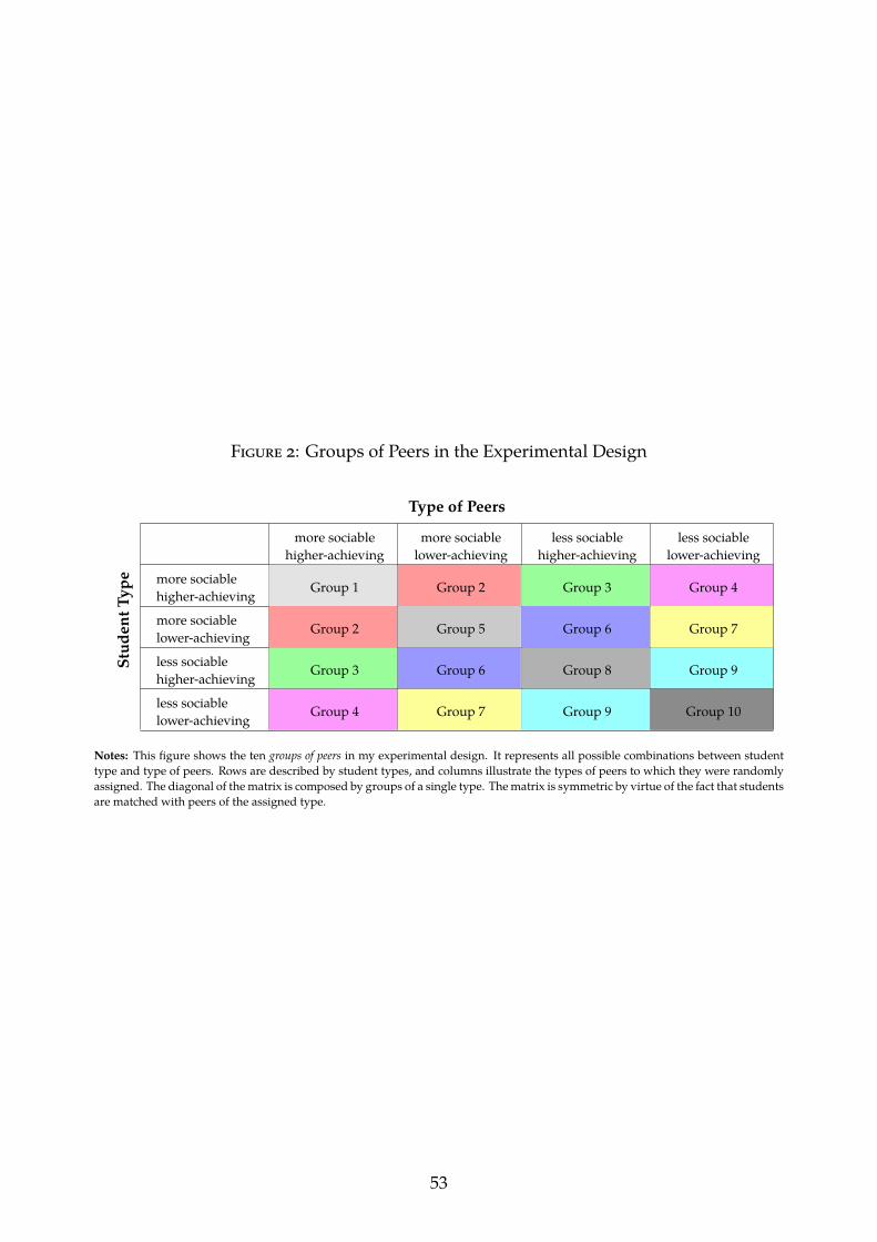
Figure 2: Groups of Peers in the Experimental Design

Type of Peers

Stud

entT

ype

more sociablehigher-achieving

more sociablelower-achieving

less sociablehigher-achieving

less sociablelower-achieving

more sociablehigher-achieving Group 1 Group 2 Group 3 Group 4

more sociablelower-achieving Group 2 Group 5 Group 6 Group 7

less sociablehigher-achieving Group 3 Group 6 Group 8 Group 9

less sociablelower-achieving Group 4 Group 7 Group 9 Group 10

Notes: This figure shows the ten groups of peers in my experimental design. It represents all possible combinations between studenttype and type of peers. Rows are described by student types, and columns illustrate the types of peers to which they were randomlyassigned. The diagonal of the matrix is composed by groups of a single type. The matrix is symmetric by virtue of the fact that studentsare matched with peers of the assigned type.

53

Figure 3: Effects of Proximity on Link Formation by Level of Sociability

Panel A: All Students

0.1

.2.3

Effe

ct

1 2 3 4 5 6 7 8 9 1 2 3 4 5 6 7 8 9

Distance

Less sociable peers More sociable peers

Panel B: Less Sociable Students Panel C: More Sociable Studentsat Baseline at Baseline

-.10

.1.2

.3

Effe

ct

1 2 3 4 5 6 7 8 9 1 2 3 4 5 6 7 8 9

Distance

Less sociable peers More sociable peers

-.10

.1.2

.3

Effe

ct

1 2 3 4 5 6 7 8 9 1 2 3 4 5 6 7 8 9

Distance

Less sociable peers More sociable peers

Notes: This figure shows the impact of distance between a pair of students on the likelihood that theybecome friends, study together, or engage in social activities such as playing or dancing. Distance is capturedby nine distance dummies, and 95% confidence intervals are displayed for all proximity effects. The figureplots the impact by treatment (more sociable peers) vs. control (less sociable peers) status in sociability. Byconstruction in the experimental design, students are at an odd distance from their treatment peers, and atan even distance from the peers of their type. Panel A presents the results for all students, Panel B for theless sociable students at baseline, and Panel C for the more sociable students at baseline. To classify studentsas more vs. less sociable, I use sociability at baseline measured by the eigenvector centrality of an aggregatesocial network of dorm preferences, friendships, study, and social partnerships. All estimations control forstrata fixed effects. Standard errors are double clustered at the student level and at the group-by-type level.

54

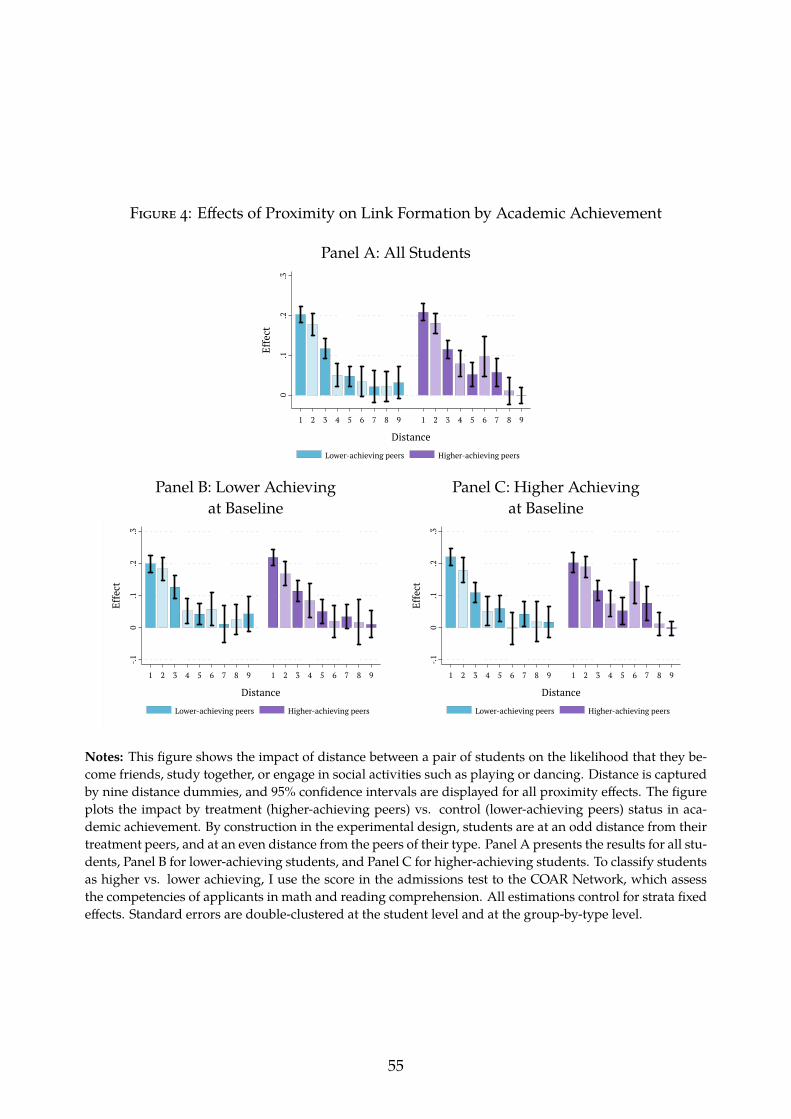
Figure 4: Effects of Proximity on Link Formation by Academic Achievement

Panel A: All Students0

.1.2

.3

Effe

ct

1 2 3 4 5 6 7 8 9 1 2 3 4 5 6 7 8 9

Distance

Lower-achieving peers Higher-achieving peers

Panel B: Lower Achieving Panel C: Higher Achievingat Baseline at Baseline

-.10

.1.2

.3

Effe

ct

1 2 3 4 5 6 7 8 9 1 2 3 4 5 6 7 8 9

Distance

Lower-achieving peers Higher-achieving peers

-.10

.1.2

.3

Effe

ct

1 2 3 4 5 6 7 8 9 1 2 3 4 5 6 7 8 9

Distance

Lower-achieving peers Higher-achieving peers

Notes: This figure shows the impact of distance between a pair of students on the likelihood that they be-come friends, study together, or engage in social activities such as playing or dancing. Distance is capturedby nine distance dummies, and 95% confidence intervals are displayed for all proximity effects. The figureplots the impact by treatment (higher-achieving peers) vs. control (lower-achieving peers) status in aca-demic achievement. By construction in the experimental design, students are at an odd distance from theirtreatment peers, and at an even distance from the peers of their type. Panel A presents the results for all stu-dents, Panel B for lower-achieving students, and Panel C for higher-achieving students. To classify studentsas higher vs. lower achieving, I use the score in the admissions test to the COAR Network, which assessthe competencies of applicants in math and reading comprehension. All estimations control for strata fixedeffects. Standard errors are double-clustered at the student level and at the group-by-type level.

55

A Supplementary Material

56

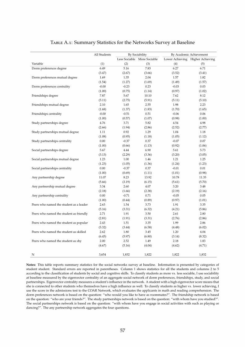
Table A.1: Summary Statistics for the Networks Survey at Baseline

All Students By Sociability By Academic AchievementLess Sociable More Sociable Lower Achieving Higher Achieving

Variable (1) (2) (3) (4) (5)Dorm preferences degree 6.49 5.16 7.83 6.27 6.71

(3.47) (2.67) (3.66) (3.52) (3.41)Dorm preferences mutual degree 1.69 1.35 2.04 1.57 1.82

(1.54) (1.27) (1.69) (1.49) (1.57)Dorm preferences centrality -0.00 -0.23 0.23 -0.03 0.03

(1.00) (0.75) (1.14) (0.97) (1.02)Friendships degree 7.87 5.67 10.10 7.62 8.12

(5.11) (2.75) (5.91) (5.11) (5.10)Friendships mutual degree 2.10 1.65 2.55 1.98 2.23

(1.68) (1.37) (1.83) (1.70) (1.65)Friendships centrality -0.00 -0.51 0.51 -0.06 0.06

(1.00) (0.57) (1.07) (0.98) (1.00)Study partnerships degree 4.76 3.71 5.82 4.54 4.98

(2.66) (1.94) (2.86) (2.52) (2.77)Study partnerships mutual degree 1.11 0.92 1.29 1.04 1.18

(1.08) (0.95) (1.18) (1.05) (1.12)Study partnerships centrality 0.00 -0.37 0.37 -0.07 0.07

(1.00) (0.66) (1.13) (0.92) (1.06)Social partnerships degree 5.67 4.44 6.90 5.61 5.73

(3.13) (2.29) (3.36) (3.20) (3.05)Social partnerships mutual degree 1.23 1.00 1.46 1.21 1.25

(1.23) (1.05) (1.36) (1.24) (1.23)Social partnerships centrality 0.00 -0.37 0.37 -0.01 0.01

(1.00) (0.69) (1.11) (1.01) (0.98)Any partnership degree 11.07 8.23 13.92 10.78 11.35

(5.66) (3.19) (6.15) (5.61) (5.70)Any partnership mutual degree 3.34 2.60 4.07 3.20 3.48

(2.18) (1.66) (2.38) (2.19) (2.16)Any partnership centrality 0.00 -0.71 0.71 -0.05 0.05

(1.00) (0.44) (0.89) (0.97) (1.01)Peers who named the student as a leader 2.63 1.54 3.73 1.91 3.35

(5.16) (3.31) (6.32) (4.21) (5.86)Peers who named the student as friendly 2.71 1.91 3.50 2.61 2.80

(2.81) (1.91) (3.31) (2.76) (2.86)Peers who named the student as popular 2.43 1.51 3.35 1.99 2.86

(5.32) (3.44) (6.58) (4.48) (6.02)Peers who named the student as skilled 2.62 1.80 3.45 1.20 4.04

(6.45) (5.97) (6.80) (3.14) (8.32)Peers who named the student as shy 2.00 2.52 1.49 2.18 1.83

(4.67) (5.16) (4.04) (4.62) (4.71)

N 3,654 1,832 1,822 1,822 1,832

Notes: This table reports summary statistics for the social networks survey at baseline. Information is presented by categories ofstudent student. Standard errors are reported in parentheses. Column 1 shows statistics for all the students and columns 2 to 5according to the classification of students by social and cognitive skills. To classify students as more vs. less sociable, I use sociabilityat baseline measured by the eigenvector centrality of an aggregate social network of dorm preferences, friendships, study, and socialpartnerships. Eigenvector centrality measures a student’s influence in the network. A student with a high eigenvector score means thatshe is connected to other students who themselves have a high influence as well. To classify students as higher vs. lower achieving, Iuse the score in the admissions test to the COAR Network, which evaluates the applicants in math and reading comprehension. Thedorm preferences network is based on the question: “who would you like to have as roommates?”. The friendship network is basedon the question: “who are your friends?”. The study partnerships network is based on the question: “with whom have you studied?”.The social partnerships network is based on the question: “with whom have you engage in social activities with such as playing ordancing?”. The any partnership network aggregates the four questions.

57

Table A.2: Correlation of Sociability and Social Skills Outcomes

Big Five Personality Traits Peers’ Perception Other measures Social Skills Index Social Skills IndexOpenness Conscientiousness Emotional Extraversion Agreeableness Leadership Friendliness Popularity Shyness of social skills Before the Intervention After the Interventipn

Stability

(1) (2) (3) (4) (5) (6) (7) (8) (9) (10) (11) (12)Academic achievement at baseline 0.090*** -0.001 0.064*** -0.014 -0.013 0.217*** 0.042** 0.105*** -0.066*** 0.047*** 0.064*** 0.042**

(0.021) (0.022) (0.022) (0.019) (0.020) (0.020) (0.016) (0.022) (0.019) (0.016) (0.017) (0.016)Sociability at baseline 0.103*** 0.061** 0.032* 0.142*** 0.120*** 0.230*** 0.359*** 0.215*** -0.103*** 0.099*** 0.139*** 0.142***

(0.024) (0.025) (0.017) (0.021) (0.017) (0.021) (0.020) (0.029) (0.021) (0.018) (0.018) (0.018)Social-fit score 0.072*** 0.022 0.001 0.063*** 0.027 0.137*** 0.073*** 0.104*** -0.113*** 0.027 0.066*** 0.046**

(0.018) (0.020) (0.020) (0.019) (0.020) (0.015) (0.016) (0.017) (0.020) (0.018) (0.017) (0.019)Interview score 0.092*** 0.073*** 0.071*** 0.091*** 0.049*** 0.068*** 0.057*** 0.049*** -0.036** 0.074*** 0.118*** 0.088***

(0.019) (0.016) (0.016) (0.018) (0.018) (0.015) (0.015) (0.017) (0.017) (0.015) (0.016) (0.015)

N 3,106 3,106 3,106 3,106 3,106 3,637 3,637 3,637 3,637 3,654 3,654 3,654

Notes: This table reports standardized estimates of an OLS regression on social skills outcomes of sociability at baseline and the score in the three tests of the admission process to the COAR Network. All regressions include school-by-grade-by-gender fixed effects.Sociability at baseline is measured by the eigenvector centrality of an aggregate social network of dorm preferences, friendships, study, and social partnerships. Eigenvector centrality is a measure of the influence of a student in the network. A student with a higheigenvector score is connected to other students who themselves have a high influence as well. Academic achievement at baseline is the score in the admission test to the COAR Network, which evaluates the applicants in math and reading comprehension. Personalitytraits correspond to the Big Five. Measures of peers’ perception correspond to the number of peers who think the student is in the top 5 of leadership, friendliness, popularity, and shyness (school-by-grade). The table presents two social skills indexes for robustness. Thefirst one is constructed using Principal Component Analysis (PCA) on all the variables that measure social skills (see Appendix C for details), excluding personality traits and measures of peers’ perception. The second index is contructed using Principal ComponentAnalysis (PCA) on all the variables that measure social skills (see Appendix C for details).

58

Table A.3: Balance Tests for the More Sociable Peers Treatment

Variable All Students Less Sociable at Baseline More Sociable at BaselineControl mean Difference Control mean Difference Control mean Difference

Admission test -0.016 0.002 -0.064 -0.024 0.058 0.028(0.019) (0.027) (0.026)

Interview score 14.065 0.009 14.053 0.019 14.082 -0.000(0.042) (0.059) (0.061)

Social-fit score 20.001 0.095 19.977 0.071 20.035 0.119(0.064) (0.088) (0.092)

Female 0.589 0.003 0.594 0.002 0.582 0.004(0.003) (0.004) (0.003)

Not poor 0.426 -0.014 0.393 -0.008 0.475 -0.020(0.014) (0.021) (0.020)

Poor 0.364 0.026* 0.378 0.034 0.344 0.019(0.015) (0.022) (0.020)

Extremely poor 0.210 -0.012 0.229 -0.026 0.182 0.001(0.012) (0.018) (0.017)

Rural 0.279 -0.014 0.315 -0.028 0.224 0.000(0.012) (0.018) (0.017)

Subsidized health insurance 0.508 0.008 0.552 -0.011 0.443 0.027(0.016) (0.022) (0.022)

Average math at baseline -0.049 0.019 -0.157 0.012 0.115 0.027(0.027) (0.037) (0.038)

Average reading at baseline -0.049 0.010 -0.169 0.041 0.134 -0.021(0.028) (0.041) (0.038)

Sociability index baseline -0.042 -0.041 -0.293 -0.033 0.333 -0.050(0.080) (0.117) (0.111)

Indegree baseline network -0.077 -0.021 -0.434 -0.003 0.460 -0.040(0.027) (0.033) (0.044)

Outdegree baseline network -0.094 0.023 -0.419 0.016 0.395 0.029(0.026) (0.027) (0.046)

Centrality baseline network 0.303 0.003 0.203 -0.002 0.453 0.008(0.003) (0.003) (0.006)

Peers’ perception leader 2.502 -0.184 1.587 -0.113 3.879 -0.257(0.151) (0.132) (0.272)

Peers’ perception friendly 2.553 -0.009 1.837 0.200** 3.631 -0.221(0.080) (0.083) (0.136)

Peers’ perception popular 2.203 0.110 1.466 0.126 3.313 0.093(0.159) (0.142) (0.285)

Peers’ perception shy 2.083 0.029 2.560 -0.131 1.366 0.192(0.144) (0.227) (0.178)

Baseline grit 43.707 -0.248 43.340 -0.171 44.251 -0.325(0.198) (0.285) (0.274)

Baseline Rosenberg scale 32.991 0.101 32.777 0.119 33.306 0.081(0.154) (0.224) (0.212)

Baseline Read the Mind 20.521 -0.060 20.224 0.184 20.960 -0.304*(0.130) (0.186) (0.180)

Multivariate F p-value 0.785 0.571 0.726

Notes: This table reports balance checks of being assigned to more sociable peers on baseline characteristics. All regressions includestrata fixed effects, control for the baseline value of the dependent variable, and include the higher-achieving peers treatment. For the2017 cohort all regressions include strata-by-classroom fixed effects. To classify students as more vs. less sociable, I use sociability atbaseline as measured by the eigenvector centrality of an aggregate social network of dorm preferences, friendships, study, and socialpartnerships. Eigenvector centrality is a measure of the influence of a student in the network. A student with a high eigenvector score isconnected to other students who themselves have a high influence as well. Eigenvector centrality is not measured for the 2017 cohort.To classify students as higher vs. lower achieving, I use the score in the admission test to the COAR Network, which evaluates theapplicants in math and reading comprehension. The control group is defined as being assigned to less sociable and lower-achievingpeers. The “F p-value” correspond to the F-statistic of the more sociable peers treatment of multivariate regressions that includeall the variables at baseline. Standard errors are clustered at the peer group type-by-type level; *** p-value<0.01, ** p-value<0.05, *p-value<0.1.

59

Table A.4: Balance Tests for the Higher-Achieving Peers Treatment

Variable All Students Lower Achieving at Baseline Higher Achieving at BaselineControl mean Difference Control mean Difference Control mean Difference

Admission test -0.163 0.013 -0.787 -0.006 0.764 0.031(0.016) (0.018) (0.026)

Interview score 8.400 -0.013 8.589 -0.011 8.117 -0.015(0.033) (0.042) (0.052)

Social-fit score 11.973 -0.061 12.161 0.012 11.693 -0.131*(0.049) (0.061) (0.077)

Female 0.575 -0.000 0.575 0.004 0.575 -0.004(0.002) (0.004) (0.003)

Not poor 0.443 0.010 0.404 0.001 0.502 0.019(0.012) (0.017) (0.018)

Poor 0.369 -0.017 0.387 -0.005 0.342 -0.030*(0.013) (0.018) (0.017)

Extremely poor 0.188 0.007 0.209 0.003 0.156 0.011(0.011) (0.016) (0.014)

Rural 0.276 -0.003 0.319 -0.021 0.212 0.014(0.013) (0.019) (0.016)

Subsidized health insurance 0.504 0.013 0.517 0.045** 0.485 -0.019(0.015) (0.021) (0.022)

Average math at baseline -0.093 0.016 -0.373 -0.023 0.319 0.053(0.023) (0.030) (0.034)

Average reading at baseline -0.064 -0.000 -0.281 -0.012 0.256 0.011(0.023) (0.032) (0.033)

Sociability index baseline -0.023 0.048 -0.065 0.060 0.040 0.038(0.059) (0.083) (0.083)

Indegree baseline network 0.008 -0.050* -0.075 -0.032 0.131 -0.068*(0.027) (0.038) (0.039)

Outdegree baseline network -0.001 -0.013 -0.016 -0.059 0.021 0.033(0.028) (0.040) (0.038)

Centrality baseline network 0.330 -0.003 0.324 -0.007 0.338 0.000(0.003) (0.004) (0.004)

Peers’ perception leader 2.493 0.006 1.930 -0.036 3.331 0.050(0.148) (0.178) (0.236)

Peers’ perception friendly 2.691 0.010 2.618 -0.001 2.801 0.021(0.078) (0.112) (0.109)

Peers’ perception popular 2.362 -0.013 2.007 -0.024 2.890 -0.006(0.158) (0.186) (0.255)

Peers’ perception shy 2.020 0.036 2.110 0.160 1.886 -0.089(0.146) (0.211) (0.203)

Baseline grit 43.568 0.158 43.330 0.431 43.921 -0.108(0.196) (0.271) (0.282)

Baseline Rosenberg scale 33.013 0.139 32.854 0.127 33.249 0.153(0.154) (0.221) (0.215)

Baseline Read the Mind 20.602 -0.265** 20.248 -0.231 21.127 -0.295(0.128) (0.180) (0.183)

Multivariate F p-value 0.810 0.857 0.625

Notes: This table reports balance checks of being assigned to higher-achieving peers on baseline characteristics. All regressions includestrata fixed effects, control for the baseline value of the dependent variable, and include the more sociable peers treatment. For the2017 cohort all regressions include strata-by-classroom fixed effects. To classify students as more vs. less sociable, I use sociability atbaseline as measured by the eigenvector centrality of an aggregate social network of dorm preferences, friendships, study, and socialpartnerships. Eigenvector centrality is a measure of the influence of a student in the network. A student with a high eigenvector score isconnected to other students who themselves have a high influence as well. Eigenvector centrality is not measured for the 2017 cohort.To classify students as higher vs. lower achieving, I use the score in the admission test to the COAR Network, which evaluates theapplicants in math and reading comprehension. The control group is defined as being assigned to less sociable and lower-achievingpeers. The “F p-value” correspond to the F-statistic of the higher-achieving peers treatment of multivariate regressions that includeall the variables at baseline. Standard errors are clustered at the peer group type-by-type level; *** p-value<0.01, ** p-value<0.05, *p-value<0.1.

60

Table A.5: Effects of Proximity on Social Interactions

All Students By Sociability By Academic AchievementLess Sociable More Sociable Lower Achieving Higher Achieving

Variable (1) (2) (3) (4) (5)Neighbor 0.161*** 0.163*** 0.141*** 0.170*** 0.151***

(0.012) (0.017) (0.017) (0.016) (0.017)More sociable peers -0.000 0.002 -0.002 0.001 -0.002

(0.001) (0.002) (0.002) (0.002) (0.001)Higher-achieving peers -0.000 -0.003* 0.002 -0.001 0.000

(0.001) (0.002) (0.002) (0.002) (0.001)Neighbor ×more sociable peers 0.037** 0.019 0.048** 0.003 0.070***

(0.015) (0.020) (0.021) (0.020) (0.022)Neighbor × higher-achieving peers 0.001 -0.022 0.035 0.011 -0.007

(0.013) (0.020) (0.022) (0.018) (0.019)

Control mean 0.11 0.11 0.11 0.11 0.11N students 6,134 1,832 1,822 3,064 3,071N pairs of students 751,758 223,719 223,147 375,896 375,862

Notes: This table reports the effect of being neighbors on the list on the likelihood that students will become friends, study togetheror engage in social activities. Effects are reported at the pair-of-students level, and include the interaction between this effect and theeffect of having more sociable peers, as well as the effect of having higher-achieving peers. All regressions include strata fixed effectsand control for whether the pair of students had any of the mentioned social interactions at baseline. To classify students as more vs.less sociable, I use sociability at baseline as measured by the eigenvector centrality of an aggregate social network of dorm preferences,friendships, study, and social partnerships. Eigenvector centrality measures a student’s influence in the network. A student with a higheigenvector score is connected to other students who themselves have a high influence as well. Eigenvector centrality is not measuredfor the 2017 cohort. To classify students as higher vs. lower achieving, I use the score in the admissions test to the COAR Network,which evaluates the applicants in math and reading comprehension. Standard errors are two-way clustered at the student and at thepeer group type-by-type level; *** p− value < 0.01, ** p− value < 0.05, * p− value < 0.1.

61

Table A.6: Reduced-Form Estimates on Social Skills Including the First-Year SociableTreatment

Big Five Personality Traits Other Measures Social SkillsExtraversion Agreeableness of social skills Index

(1) (2) (3) (4)Panel A: All Students

More sociable peers 0.067** 0.066** 0.048* 0.067**(0.031) (0.032) (0.029) (0.028)

More sociable peers (first-years) -0.094 0.010 0.045 0.035(0.063) (0.067) (0.061) (0.056)

Higher-achieving peers -0.005 -0.008 -0.013 -0.009(0.027) (0.028) (0.025) (0.024)

N 4,826 4,826 6,021 6,021

Panel B: Less Sociable First-Year Students at BaselineMore sociable peers (first-years) -0.044 -0.054 0.083 0.064

(0.110) (0.122) (0.102) (0.093)Higher-achieving peers 0.079 -0.098 -0.097 -0.064

(0.095) (0.087) (0.075) (0.073)

N 825 825 1,172 1,172Panel C: More Sociable First-Year Students at Baseline

More sociable peers (first-years) -0.120 0.065 0.005 0.007(0.093) (0.092) (0.082) (0.080)

Higher-achieving peers 0.074 0.052 -0.050 -0.018(0.083) (0.075) (0.073) (0.068)

N 895 895 1,195 1,195

Notes: This table reports the effect of being assigned to more sociable and higher-achieving peers identified at baseline based on personality traits, andsocial skills outcomes. All regressions include strata fixed effects and control for the baseline value of the dependent variable. For the 2017 cohort allregressions include strata-by-classroom fixed effects. To classify students as more vs. less sociable for the 2015-16 cohorts, I use sociability at baselineas measured by the eigenvector centrality of an aggregate social network of dorm preferences, friendships, study, and social partnerships. Eigenvectorcentrality measures a student’s influence in the network. A student with a high eigenvector score is connected to other students who themselves havea high influence as well. To classify students as more vs. less sociable for the first-year, I use the social-fit score in the admission test that evaluates thestudents in empathy, leadership, and teamwork. To classify students as higher vs. lower achieving, I use the score in the admissions test to the COARNetwork, which evaluates the applicants in math and reading comprehension. The control group is defined as being assigned to less sociable and lower-achieving peers. Personality traits correspond to the Big Five. Measures of peers’ perceptions correspond to the number of peers who think the studentis in the top five of leadership, friendliness, popularity, and shyness (school-by-grade). The table presents two social skills indexes for robustness. Thefirst is constructed using PCA on all the variables that measure social skills (see Appendix C for details), excluding personality traits and measures ofpeers’ perceptions. The second index is constructed using PCA on all the variables that measure social skills (see Appendix C for details). The table alsoreports the RI p-values of each treatment. The treatments were randomly reassigned on 1,000 permutations of students. Each outcome variable was thenregressed on the reassigned treatment indicators. The true coefficients were then compared to the distribution of coefficients induced by reassignment inorder to generate the RI p-values. The last row reports the p-value of equal treatment effects of more sociable peers for less sociable and more sociablestudents at baseline. Standard errors are clustered at the peer group type-by-type level; *** p-value<0.01, ** p-value<0.05, * p-value<0.1.

62

Table A.7: Reduced-Form Estimates on Cognitive Skills Including the First-Year SociableTreatment

Grades Test ScoresMath Reading Math Reading

(1) (2) (3) (4)Panel A: All Students

More sociable peers 0.004 0.038 -0.036 0.021(0.036) (0.039) (0.025) (0.033)

More sociable peers (first-years) -0.003 0.012 -0.008 0.016(0.061) (0.056) (0.046) (0.052)

Higher-achieving peers -0.041 -0.005 -0.028 -0.038(0.028) (0.030) (0.021) (0.027)

N 4,330 4,333 4,337 4,359Panel B: Lower-Achieving Students at Baseline

More sociable peers -0.005 0.085 -0.047 0.024(0.050) (0.053) (0.033) (0.045)

More sociable peers (first-years) -0.059 0.016 -0.025 0.002(0.084) (0.076) (0.061) (0.077)

Higher-achieving peers -0.098** -0.075* -0.060** -0.070*(0.039) (0.042) (0.028) (0.037)

N 2,158 2,159 2,159 2,172Panel C: Higher-Achieving Students at Baseline

More sociable peers 0.012 -0.009 -0.024 0.019(0.051) (0.055) (0.037) (0.049)

More sociable peers (first-years) 0.052 -0.011 0.008 0.025(0.091) (0.082) (0.070) (0.068)

Higher-achieving peers 0.005 0.061 -0.004 -0.010(0.039) (0.041) (0.031) (0.038)

N 2,172 2,174 2,178 2,187

Notes: This table reports the effect of being assigned to more sociable and higher-achieving peers identified at baseline based on personality traits, andsocial skills outcomes. All regressions include strata fixed effects and control for the baseline value of the dependent variable. For the 2017 cohort allregressions include strata-by-classroom fixed effects. To classify students as more vs. less sociable for the 2015-16 cohorts, I use sociability at baselineas measured by the eigenvector centrality of an aggregate social network of dorm preferences, friendships, study, and social partnerships. Eigenvectorcentrality measures a student’s influence in the network. A student with a high eigenvector score is connected to other students who themselves havea high influence as well. To classify students as more vs. less sociable for the first-year, I use the social-fit score in the admission test that evaluates thestudents in empathy, leadership, and teamwork. To classify students as higher vs. lower achieving, I use the score in the admissions test to the COARNetwork, which evaluates the applicants in math and reading comprehension. The control group is defined as being assigned to less sociable and lower-achieving peers. Personality traits correspond to the Big Five. Measures of peers’ perceptions correspond to the number of peers who think the studentis in the top five of leadership, friendliness, popularity, and shyness (school-by-grade). The table presents two social skills indexes for robustness. Thefirst is constructed using PCA on all the variables that measure social skills (see Appendix C for details), excluding personality traits and measures ofpeers’ perceptions. The second index is constructed using PCA on all the variables that measure social skills (see Appendix C for details). The table alsoreports the RI p-values of each treatment. The treatments were randomly reassigned on 1,000 permutations of students. Each outcome variable was thenregressed on the reassigned treatment indicators. The true coefficients were then compared to the distribution of coefficients induced by reassignment inorder to generate the RI p-values. The last row reports the p-value of equal treatment effects of more sociable peers for less sociable and more sociablestudents at baseline. Standard errors are clustered at the peer group type-by-type level; *** p-value<0.01, ** p-value<0.05, * p-value<0.1.

63

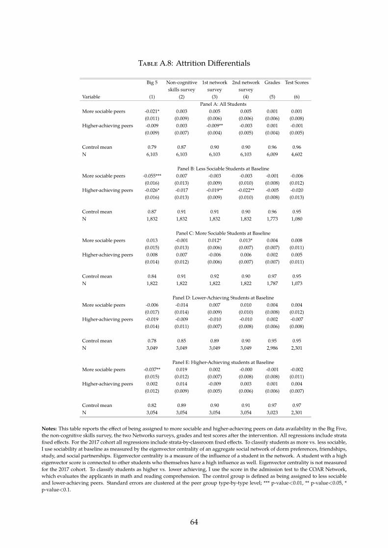
Table A.8: Attrition Differentials

Big 5 Non-cognitive 1st network 2nd network Grades Test Scoresskills survey survey survey

Variable (1) (2) (3) (4) (5) (6)Panel A: All Students

More sociable peers -0.021* 0.003 0.005 0.005 0.001 0.001(0.011) (0.009) (0.006) (0.006) (0.006) (0.008)

Higher-achieving peers -0.009 0.003 -0.009** -0.003 0.001 -0.001(0.009) (0.007) (0.004) (0.005) (0.004) (0.005)

Control mean 0.79 0.87 0.90 0.90 0.96 0.96N 6,103 6,103 6,103 6,103 6,009 4,602

Panel B: Less Sociable Students at BaselineMore sociable peers -0.055*** 0.007 -0.003 -0.003 -0.001 -0.006

(0.016) (0.013) (0.009) (0.010) (0.008) (0.012)Higher-achieving peers -0.026* -0.017 -0.019** -0.022** -0.005 -0.020

(0.016) (0.013) (0.009) (0.010) (0.008) (0.013)

Control mean 0.87 0.91 0.91 0.90 0.96 0.95N 1,832 1,832 1,832 1,832 1,773 1,080

Panel C: More Sociable Students at BaselineMore sociable peers 0.013 -0.001 0.012* 0.013* 0.004 0.008

(0.015) (0.013) (0.006) (0.007) (0.007) (0.011)Higher-achieving peers 0.008 0.007 -0.006 0.006 0.002 0.005

(0.014) (0.012) (0.006) (0.007) (0.007) (0.011)

Control mean 0.84 0.91 0.92 0.90 0.97 0.95N 1,822 1,822 1,822 1,822 1,787 1,073

Panel D: Lower-Achieving Students at BaselineMore sociable peers -0.006 -0.014 0.007 0.010 0.004 0.004

(0.017) (0.014) (0.009) (0.010) (0.008) (0.012)Higher-achieving peers -0.019 -0.009 -0.010 -0.010 0.002 -0.007

(0.014) (0.011) (0.007) (0.008) (0.006) (0.008)

Control mean 0.78 0.85 0.89 0.90 0.95 0.95N 3,049 3,049 3,049 3,049 2,986 2,301

Panel E: Higher-Achieving students at BaselineMore sociable peers -0.037** 0.019 0.002 -0.000 -0.001 -0.002

(0.015) (0.012) (0.007) (0.008) (0.008) (0.011)Higher-achieving peers 0.002 0.014 -0.009 0.003 0.001 0.004

(0.012) (0.009) (0.005) (0.006) (0.006) (0.007)

Control mean 0.82 0.89 0.90 0.91 0.97 0.97N 3,054 3,054 3,054 3,054 3,023 2,301

Notes: This table reports the effect of being assigned to more sociable and higher-achieving peers on data availability in the Big Five,the non-cognitive skills survey, the two Networks surveys, grades and test scores after the intervention. All regressions include stratafixed effects. For the 2017 cohort all regressions include strata-by-classroom fixed effects. To classify students as more vs. less sociable,I use sociability at baseline as measured by the eigenvector centrality of an aggregate social network of dorm preferences, friendships,study, and social partnerships. Eigenvector centrality is a measure of the influence of a student in the network. A student with a higheigenvector score is connected to other students who themselves have a high influence as well. Eigenvector centrality is not measuredfor the 2017 cohort. To classify students as higher vs. lower achieving, I use the score in the admission test to the COAR Network,which evaluates the applicants in math and reading comprehension. The control group is defined as being assigned to less sociableand lower-achieving peers. Standard errors are clustered at the peer group type-by-type level; *** p-value<0.01, ** p-value<0.05, *p-value<0.1.

64

Table A.9: Reduced Form Estimates on Personality Traits (Accounting for Attrition)

Dependent variable: Attrition Big Five Big Five Personality TraitsOpenness Conscientiousness Emotional Stability Extraversion Agreeableness

(1) (2) (3) (4) (5) (6)More sociable peers -0.007 0.077* 0.033 0.051 0.084* 0.108**

(0.016) (0.046) (0.048) (0.043) (0.046) (0.046)Higher-achieving peers -0.025 -0.041 0.070 0.036 -0.061 0.017

(0.016) (0.045) (0.046) (0.043) (0.046) (0.046)

Control mean 0.87 -0.04 -0.04 -0.08 -0.01 -0.05N 1,622 1,370 1,370 1,370 1,370 1,370

Notes: This table reports the effect of being assigned to more sociable and higher achieving peers identified at baseline on personality traits. Effects are presented for the less sociable students at baselineonly, and account for attrition in the Big Five. All regressions include strata fixed effects and control for the baseline value of the dependent variable. For the 2017 cohort all regressions include strata-by-classroom fixed effects. To classify students as more vs. less sociable, I use sociability at baseline as measured by the eigenvector centrality of an aggregate social network of dorm preferences, friendships,study, and social partnerships. Eigenvector centrality is a measure of the influence of a student in the network. A student with a high eigenvector score is connected to other students who themselveshave a high influence as well. Eigenvector centrality is not measured for the 2017 cohort. To classify students as higher vs. lower achieving, I use the score in the admission test to the COAR Network,which evaluates the applicants in math and reading comprehension. The control group is defined as being assigned to less sociable and lower-achieving peers. Personality traits correspond to the BigFive. Standard errors are clustered at the peer group type-by-type level; *** p-value<0.01, ** p-value<0.05, * p-value<0.1.

65

Table A.10: Treatments and Outcomes Available by Cohort

Treatments OutcomesSocial Skills Cognitive Skills

More sociable peers 2015, 2016 2016Higher-achieving peers 2015, 2016, 2017 2016, 2017Complementarity 2015, 2016 2016

Figure A.1: Figure Appendix: Dorm Structure

School in Lima

School in Piura School in Cusco

Notes: This figure displays pictures of the dorms for the schools in Lima, Piura, and Cusco.

66

Figure A.2: Correlation of Cognitive and Social Skills

-2-1

01

23

4

A

cade

mic

Ach

ieve

men

tBe

fore

the

Inte

rven

tion

-2 -1 0 1 2 3 4

Social Skills IndexBefore the Intervention

achievement=0.00+0.11*socialskills

Notes: This figure shows a scatter plot of academic achievement and sociability at baseline for the 2015-16cohorts by student type. A one standard deviation of the social skills index predicts an increase in 0.11standard deviations of academic achievement at baseline.

67

Figure A.3: Correlation of the Sociability Index Before and After the Intervention

-2-1

01

23

Soci

al S

kills

Inde

xA

fter

the

Inte

rven

tion

-2 0 2 4

Social Skills IndexBefore the Intervention

socialskillst=0.00+0.42*socialskillst-1

Notes: This figure shows a scatter plot and the linear prediction of the sociability index before and after theintervention. A one standard deviation of the social skills index before the intervention predicts an increaseof 0.42 in the social skills index after the intervention.

68

B Use of the Lists to Allocate Students to Dorms and Classrooms

This section explains in detail how the order of students on the lists determines their al-location to dormitories. To start, recall the simple two-type example in which studentswere either H and L. As described in section 3.3.2, this case allows for three groups ofcombined types: Group 1 (only Hs), Group 2 (a mixed group of Hs and Ls), and Group 3(only Ls). Let us assume that the random ordering of the groups on the list is: Group 1-Group 3-Group 2. For the purpose of illustration, I will assume that there are 12 students,four in each group. After numbering the students by type, the order on the list would bethe following: H1 −H2 −H3 −H4 − L1 − L2 − L3 − L4 −H5 − L5 −H6 − L6. Notice thaton the list, the order of the students in Group 2 alternates the type of student in the formH-L.

Figure B.1 shows an illustrative example of how the lists were used to allocate studentsto dorms and classrooms. Panel A describes the allocation when each room holds fourstudents, Panel B when dorm rooms hold three students and Panel C for a big dorm roomof 12 students. The order on the list is used to determine the allocation. When dormrooms hold four students, dorms and peer group types have the same size so there is perfectcompliance with the initial allocation. Yet, when dorm rooms hold three students, the firstthree students of typeH –who were assigned to Group 1 (onlyHs)—are allocated to room1. The fourth student assigned to Group 1 is assigned to a room with two students whoare type L. Notice that in this case there is no perfect compliance. In the big dorm, allstudents H1 − H4 are in beds close to each other. However, students H3 and H4 are alsoclose to students of type L, while students H1 and H2 are surrounded only by peers whoare type H .

69

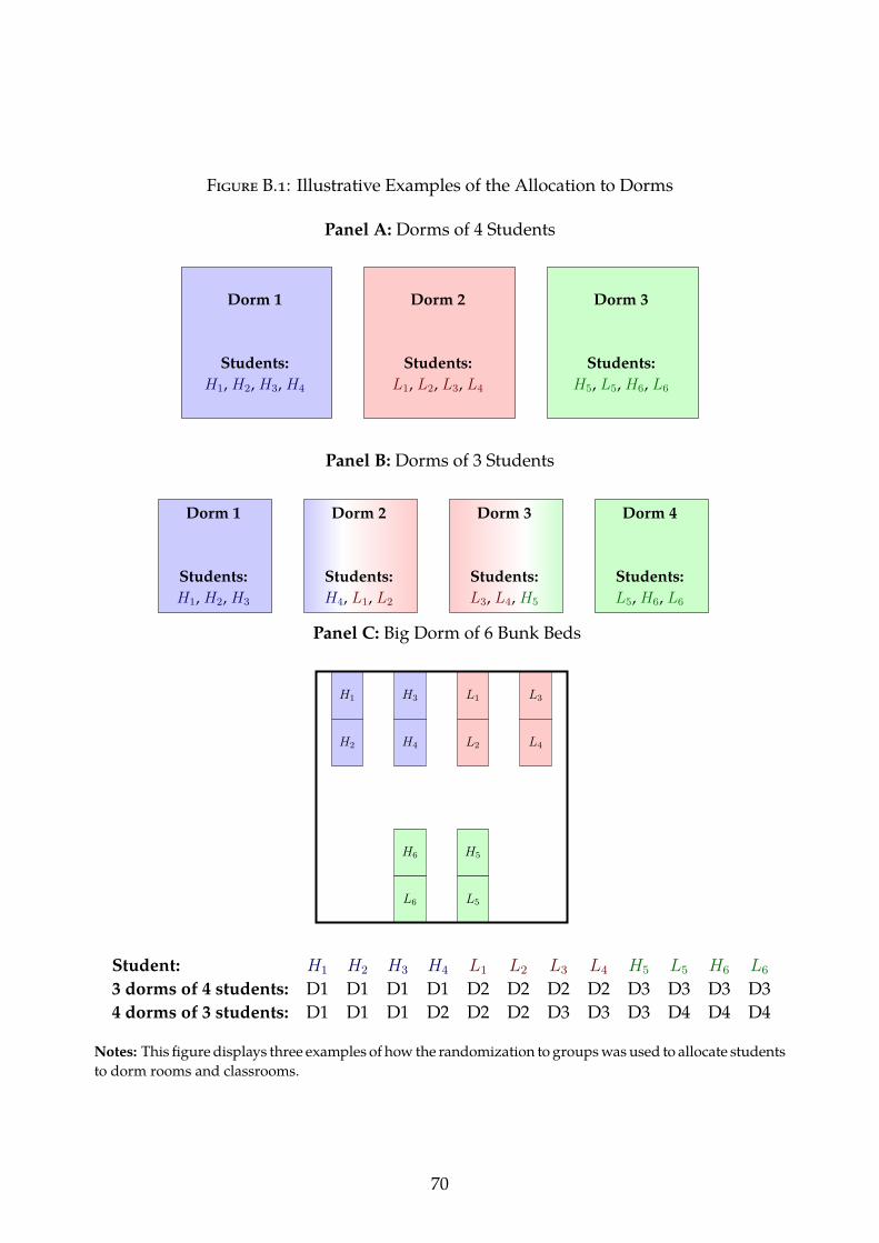
Figure B.1: Illustrative Examples of the Allocation to Dorms

Panel A: Dorms of 4 Students

Dorm 1

Students:H1, H2, H3, H4

Dorm 2

Students:L1, L2, L3, L4

Dorm 3

Students:H5, L5, H6, L6

Panel B: Dorms of 3 Students

Dorm 1

Students:H1, H2, H3

Dorm 2

Students:H4, L1, L2

Dorm 3

Students:L3, L4, H5

Dorm 4

Students:L5, H6, L6

Panel C: Big Dorm of 6 Bunk Beds

H1

H2

H3

H4

L1

L2

L3

L4

L6

H6

L5

H5

Student: H1 H2 H3 H4 L1 L2 L3 L4 H5 L5 H6 L6

3 dorms of 4 students: D1 D1 D1 D1 D2 D2 D2 D2 D3 D3 D3 D34 dorms of 3 students: D1 D1 D1 D2 D2 D2 D3 D3 D3 D4 D4 D4

Notes: This figure displays three examples of how the randomization to groups was used to allocate studentsto dorm rooms and classrooms.

70

C Psychological Tests

This section describes in detail the psychological tests that were used to construct the so-ciability index.

In addition to the Big Five personality traits and the peers’ perceptions measures de-scribed in section 5.1, the tests used to construct the sociability index are:

• Altruism: The altrusim self-reported scale was developed by Rushton et al. (1981).The test used in the COAR network is composed of 17 items. The score on the testis found to predict criteria such as peer ratings of altruism, completing an organdonor card, and paper-and-pencil measures of prosocial orientation (Rushton et al.,1981). More recent evidence shows that the score on the test is related to spontaneoussmiles—which is an important signal in the formation and maintenance of cooper-ative relationships (Mehu et al., 2007). Likewise, there is evidence that the score inthe test is related to charity giving but not to blood donor donation behavior (Ottoand Bolle, 2011).

• Leadership: The leadership scale corresponds to the leader behavior questionnairedeveloped in Spanish by Castro-Solano (2007). It is based on the theory of Yukl(2013). The scale measures three components of leadership: (1) behaviors guidedtowards tasks, (2) behaviors guided towards others, and (3) behaviors guided to-wards changes. In my data, there is a positive correlation between the score on thescale and the number of peers who perceived the subject as a leader.

• Empathy: The empathy scale corresponds to the Basic Empathy Scale developed byJolliffe and Farrington (2006). The scale is composed of two factors: cognitive andemotional empathy. The scale has been validated in other contexts: when appliedto adults (Carre et al., 2013) and the Spanish version of it (Villadangos et al., 2016).It has also been affirmed that students who report higher scores in socially aversivepersonalities (psychopathy, narcissism, and Machiavellianism) have a low score onthe scale (Wai and Tiliopoulos, 2012). Likewise, Gambin and Sharp (2018) show thata low score on the test is associated with guilt and depressive symptoms.

• Intercultural Sensitivity: This 24-item scale of intercultural sensitivity was devel-oped by Chen and Starosta (2000). The authors define intercultural sensitivity as:“a person’s ability to develop a positive emotion towards understanding and appreciatingcultural differences that promotes appropriate and effective behavior in intercultural com-munication.” The scale is composed of two factors: positive and negative reactionsto intercultural interactions. Evidence shows that there is a positive correlation be-tween intercultural sensitivity and compassion in nurses (Arli and Bakan, 2018), thatAmerican student scores depend on religious affiliation and the number of times

71

they have traveled outside the US (Gordon and Mwavita, 2018), and that Iranianuniversity students have demonstrated a strong relationship between interculturalsensitivity and ethnic background.

• Emotional Intelligence: Emotional intelligence is defined as individuals’ ability torecognize their own emotions and those of others, discern between different feel-ings and label them appropriately, use emotional information to guide thinking andbehavior, and manage and/or adjust emotions to adapt to environments or achieveone’s goal(s) (Colman, 2009). The emotional intelligence test corresponds to the scaledeveloped by Law et al. (2004). The test is composed of 16 items and has four fac-tors: self-emotional appraisal, uses of emotion, regulation of emotion, and others’emotional appraisal.

• The Read the Mind in the Eyes Test: The objective of this test is to assess howwell people can read others’ emotions just by looking at pictures of their eyes. Itis a multiple choice test with 36 items. For each item, the respondent has to iden-tify the corresponding emotion expressed in a pair of eyes; four choices are givenfor each question. According to Deming (2017), this test is a reliable measure ofsocial skills since it is positively correlated with performance in groups (Declerckand Bogaert, 2008). However, this measure could potentially have problems dueto the cultural differences between the context where the test was developed andthe context of my study. In particular, according to the website Lab in the Wild:socialintelligence.labinthewild.org, the test was developed in Great Britainand the images were taken from British magazines in the 1990s. Therefore, the testmay not produce accurate results when administered to people who are not nativespeakers of English or those who come from cultures that are very different fromBritain’s.

While not part of the construction of the sociability index, students completed otherassessments:

• Achievement Goals: Achievement goals are conceptualized as cognitive–dynamicaims that focus on competence. Students answered the The Achievement Goal Ques-tionnaire (J. Elliot and Murayama, 2008). The test is composed of 12 items and hasfour factors: mastery approach goal items, mastery avoidance goal items, perfor-mance approach goal items, and performance avoidance goal items. The last twoitems are related to goals in comparison with peers.

72

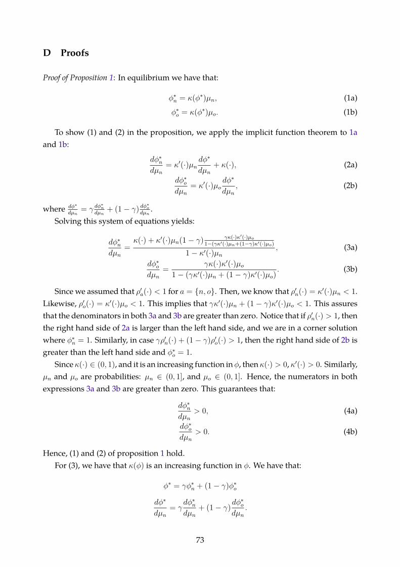
D Proofs

Proof of Proposition 1: In equilibrium we have that:

φ∗n = κ(φ∗)µn, (1a)

φ∗o = κ(φ∗)µo. (1b)

To show (1) and (2) in the proposition, we apply the implicit function theorem to 1aand 1b:

dφ∗ndµn

= κ′(·)µndφ∗

dµn+ κ(·), (2a)

dφ∗odµn

= κ′(·)µodφ∗

dµn, (2b)

where dφ∗

dµn= γ dφ

∗n

dµn+ (1− γ) dφ

∗o

dµn.

Solving this system of equations yields:

dφ∗ndµn

=κ(·) + κ′(·)µn(1− γ) γκ(·)κ′(·)µo

1−(γκ′(·)µn+(1−γ)κ′(·)µo)

1− κ′(·)µn, (3a)

dφ∗odµn

=γκ(·)κ′(·)µo

1− (γκ′(·)µn + (1− γ)κ′(·)µo). (3b)

Since we assumed that ρ′a(·) < 1 for a = {n, o}. Then, we know that ρ′n(·) = κ′(·)µn < 1.Likewise, ρ′o(·) = κ′(·)µo < 1. This implies that γκ′(·)µn + (1− γ)κ′(·)µo < 1. This assuresthat the denominators in both 3a and 3b are greater than zero. Notice that if ρ′n(·) > 1, thenthe right hand side of 2a is larger than the left hand side, and we are in a corner solutionwhere φ∗n = 1. Similarly, in case γρ′n(·) + (1− γ)ρ′o(·) > 1, then the right hand side of 2b isgreater than the left hand side and φ∗o = 1.

Sinceκ(·) ∈ (0, 1), and it is an increasing function inφ, thenκ(·) > 0, κ′(·) > 0. Similarly,µn and µo are probabilities: µn ∈ (0, 1], and µo ∈ (0, 1]. Hence, the numerators in bothexpressions 3a and 3b are greater than zero. This guarantees that:

dφ∗ndµn

> 0, (4a)

dφ∗odµn

> 0. (4b)

Hence, (1) and (2) of proposition 1 hold.For (3), we have that κ(φ) is an increasing function in φ. We have that:

φ∗ = γφ∗n + (1− γ)φ∗o

dφ∗

dµn= γ

dφ∗ndµn

+ (1− γ)dφ∗o

dµn.

73

Since γ ∈ (0, 1), and dφ∗ndµn

> 0, dφ∗o

dµn> 0, then dφ∗

dµn> 0. Since κ(φ) is an increasing function in

φ, then dκ(φ∗)dµn

= κ′(·) dφ∗dµn

> 0.

Proof of corollary 1: The likelihood that the agent invests in equilibrium is given byG(φ∗a). Since G(·) is a c.d.f. with no flat regions then, G(·) is a strictly increasing functionand φ∗a(·) increases with µn for a = {n, o}. Hence, the agent invests more in both types ofactivities.

Proof of Proposition 2: Under the assumption of social success, for less sociable studentsµn(l, l) < µn(l, h). By applying proposition 1 and corollary 1 we obtain the result. Formore sociable students µn(h, l) = µn(h, h), and therefore they do not experience changesin self-confidence or investment decisions.

Proof of Proposition 3: Under the assumption of cognitive success, for lower-achievingstudents µn(l, h) < µn(l, l). By applying proposition 1 and corollary 1 we obtain the result.For higher-achieving students µn(h, l) = µn(h, h), and therefore they do not experiencechanges in self-confidence or investment decisions.

74

E Network Formation Model

This section explores the impact of the allocation of students on network formation, in-cluding dependencies in the formation of links.

E.1 Exponential Random Graph Models (ERGM)

For the descritpion of this section, I follow Handcock et al. (2018) and Handcock et al.(2016)21. Exponential random graph models (ERGMs) are a family of statistical models,which are suitable for the analysis of data on social networks. The assumption behindthese models is that the structure of a network graph Y can be explained by any statisticg(Y ), such as the number of ties, centrality measures, and so on. The ERGM assigns aprobability to graphs on the basis of these statistics. The general form for an ERGM canbe written as:

P (Y = y) =exp(θ′g(y))

k(θ)(5)

where Y is the random variable for the state of the network —with realization y—, andg(y) is a vector of statistics for the network; θ is a vector of associated coefficients to thosestatistics, and k(θ) is a normalizing constant that represents the quantity in the numeratorover all possible realizations of network Y .

Equation 5 can be re-expressed in terms of the conditional log-odds of a single tie be-tween two students as:

logit(Yij = 1|ycij) = θ′δ(yij)),

where Yij is the random variable for the state of the dyad between students i and j; ycijrepresent all the other dyads in the network other than yij . The vector δ(yij)) contains the“change statistic” for each model term g(y).

δ(yij) = g(y+ij)− g(y−ij)

where y+ij gets determined by ycij and setting yij to 1, and y−ij is defined by ycij and set-tinh yij set to 0. That is, δ(yij)) equals the value of g(y) when yij = 1 minus the value ofg(y) when yij = 0, but all other dyads are as in g(y). Therefore the coefficient θ can beinterpreted as the log-odds of an individual tie conditional on all others.

I perform the estimation using the package statnet in R22. In my analysis, I consider thefollowing set of statistics as part of the set g(Y ): the number of edges in the network, thenumber of neighbors, and the interaction between the number of neighbors with treat-ments and baseline characteristics. I estimate a separate model by the baseline classifica-

21This tutorial can be accessed: https://statnet.org/trac/raw-attachment/wiki/Sunbelt2016/

ergm_tutorial.html.22http://statnet.org/

75

tion of: (i) less and more sociable students, and (ii) lower- and higher- achieving students.

g1(y) = {edges, neighbors× treatments× baseline}

In addition to these terms, I estimate a second model that includes a geometrically-weighededgewise shared partner term that accounts for link dependencies.

Figures E.1 and E.2 show the estimates for the less sociable students, and lower-achievingstudents, respectively. The figure presents three panels, one for each coefficient. Panel Ashows the results for the neighbor, and panels B and C for heteroeneous effects of neigh-bors by each treatment status. Overall, I find very similar estimates regardless of includingor not the link-dependencies term.. Therefore, the conclusions of social interactions arerobust to link dependencies. There is a substantial impact of being neighbors on the likeli-hood of forming social interactions and there are no heterogeneous impacts by treatmentneither for the less sociable nor the lower-achieving students.

76

Figure E.1: Estimates of ERGM by Baseline Sociability

Panel A: The coefficient of neighborsfor less sociable students

-1.00

0.00

1.00

2.00

3.00

Edges Decaying

Panel B: The coefficient of neighbors Panel C: The coefficient of neighbors×more sociable peers × higher-achieving peers

for less sociable students for less sociable students

-0.50

0.00

0.50

Edges Decaying

-1.00

-0.50

0.00

0.50

Edges Decaying

Notes: This figure shows the estimates of an ERGM for each network. 95% confidence intervals are dis-played for all estimates. The model includes the number of edges in the graph, and the neighbor coefficientinteracted with treatments status and baseline characteristics of sociability. The plot presents estimates fortwo models: one with edges (blue circles) without link dependencies, and a second model including linkdependencies with a decaying geometrically-weighed edgewise shared partner term of 0.1 (purple circles).The network aggregates whether students are friends, study together, or engage in social activities such asplaying or dancing.

77

Figure E.2: Estimates of ERGM by Baseline Academic Achievement

Panel A: The coefficient of neighborsfor lower-achieving students

-1.00

0.00

1.00

2.00

3.00

Edges Decaying

Panel B: The coefficient of neighbors Panel C: The coefficient of neighbors×more sociable peers × higher-achieving peers

for lower-achieving students for lower-achieving students

-0.50

0.00

0.50

Edges Decaying

-1.00

-0.50

0.00

0.50

Edges Decaying

Notes: This figure shows the estimates of an ERGM for each network. 95% confidence intervals are dis-played for all estimates. The model includes the number of edges in the graph, and the neighbor coefficientinteracted with treatments status and baseline characteristics of sociability. The plot presents estimates fortwo models: one with edges (blue circles) without link dependencies, and a second model including linkdependencies with a decaying geometrically-weighed edgewise shared partner term of 0.1 (purple circles).The network aggregates whether students are friends, study together, or engage in social activities such asplaying or dancing.

78