Embed Size (px)
Citation preview


Tạp chí Khoa học và Công nghệ
SPECIAL ISSUE ON THE 49th ESTABLISHMENT OF COLLEGE OF TECHNOLOGY – TNU
(19/8/1965 – 19/8/20140
Content Page
The Quang Phan, Dung Thi Quoc Nguyen, Thao Thi Phuong Phan - Effects of Workpiece Hardness on Hard
Turned Surfaces of Alloy Steels 3
Lanh Van Nguyen, Loc Bao Dam - Direct MRAS based an Adaptive Control System for Twin Rotor MIMO
System 9
Nguyen Minh Y, Thang N.Pham and Toan H. Nguyen - A new approach for enery saving to household
customers based smartgrid technologies 15
Dinh Thi Gia, Tuan Manh Tran, Son Que Tran - Direct mras with safe constraints applied for two-wheeled
mobile robot 21
Phong Tien Le, Minh Duc Ngo - Research on designing an energy management system
for isolated pv source 29
Phong Tien Le, Huong Thi Mai Nguyen, Hung Tien Nguyen - Control of grid-connected solar power systems
with interleaved flyback converters 37
Nam Hoai Nguyen, Trinh Thi Minh Nguyen - A new training procedure for a class of recurrent neural networks 43
Cam Thi Hong Nguyen, Trang Van Nguyen, Pi Ngoc Vu - A new study on optimum calculation of partial transmission ratios of coupled planetary gear sets 47
Thuy Thi Thu Nguyen - Establishment of a database of emission factors for atmospheric pollutants from steel
rolling 51
Duy Tien Nguyen, Binh Hoang Lam, Son Hung Lam, Huy Phuong Nguyen - Dissolved Oxygen Control of the Activated Sludge Wastewater Treatment Process Using Hedge AlgebraicControl 57
Khuyen Thi Minh Pham, Yen Thi Mai Pham - Supply chain management for colleges/universities: solutions to
improve the efficiency of science and technology transfer 63
Thao Thi Phuong Phan, Thinh Duc Nguyen, Oanh Thi Lam Nguyen - Design and fabrication of robotic bluetooth cleaner 69
Thinh Duc Nguyen, Tuan Anh Vu, Du Van Nguyen- Caculation analysis and design for construction of solar
engine model 73
Ha Thi Thu Phan, Thao Thi Phuong Phan - Effect of annealing treatment on high strain rate behavior of
Graphene reinforced Polyurethane composites 77
Thuy Thi Hong Truong, Nga Thi Hong Do -Application of neural networks or diagnosis of hepatitis 81
Huy Ngoc Vu, Tuan Manh Tran, Huong Thi Mai Nguyen, Hung Tien Nguyen - Robust control of dc motors 87
Huy Ngoc Vu, Tuan Manh Tran, Huong Thi Mai Nguyen, Hung Tien Nguyen - Thyristor-based digital control of dc motors 93
Kien Ngoc Vu, Du Huy Dao, Cong Huu Nguyen - Research to improve the model order reduction algorithm 101
Viet Quoc Vu - Improving the efficiency of conventional drinking-water-treatment processes in the removal of
arsenic 107
Huyen Vu Xuan Dang, Hanh Vu Bich Dang, Amira Abdelrasoul, Huu Doan, Dan Phuoc Nguyen -
Assessment of treated latex wastewater reuse for perennial tree irrigation on ground water quality 111
Huyen Vu Xuan Dang, Huyen Thi Bich Trinh, Hanh Vu Bich Dang, Dan Phuoc Nguyen - Studying on toxicity of treated latex wastewater to plant perennial tree – a case study in Binh Duong, VietNam 117
Journal of Science and Technology 127(13)
2014

The Quang Phan et al Journal of SCIENCE and TECHNOLOGY 127(13): 3 - 8
3
EFFECTS OF WORKPIECE HARDNESS ON HARD TURNED SURFACES OF ALLOY STEELS
The Quang Phan, Dung Thi Quoc Nguyen* and Thao Thi Phuong Phan
University of Technology - TNU
ABSTRACT
Nowadays, hard turning is widely applied in Vietnam industry and it is usually the finished
operation so the quality of the machined surface plays a very important role to the use today and in
the future. This paper presents results of a research on hard turning of 9XC and X12M alloy steels
to explore the influence of workpiece’s hardness on machined surface roughness and topography
at selected cutting conditions. It is evident that the surface roughness was directly proportional to
the increase of the workpiece’s hardness from HRC = around 50 to higher than 60. Moreover,
lower hardness resulted in worse surface roughness. Even though when the cutting speed increased
by twice, the best surface roughness still achieved at the workpiece’s hardness of HRC= around
50. The cause is predicted to be involved with a change in chip/ rake face interactions depending
on workpiece’s hardness and tools wear.
Keywords: Hard turning, furface roughness, topography, workpiece, tool wear.
INTRODUCTION*
Precision machined components can be
manufactured by hard turned or ground
operations. Surface integrity is a qualitative
and quantitative description of both the
surface and subsurface component including
surface topography, surface and subsurface
hardness, microstructure and residual stresses,
etc. The work of Schwach and Gue [1] used a
stylus instrument to measured surface
roughness created by hard turn stated that
surface roughness decreased when feed rate
reduced. Decreasing feed rates makes the
surface residual stress more compressive and
its maximal one closer to the surface.
Moreover, tools wear increased surface
roughness except at moderate mode. Sharp
cutting tool is recommended for hard turn to
get better surface integrity. Chou [2] stated
that fine structure of the workpiece PM M50
steel resulted in lower wear rate by delay of
delamination wear and this effect is much
stronger in intermittent cutting.
Barbacki and co-workers [3] carried out
experiments to compare the microstructural
* Tel: 0915308818; Email: [email protected]
changes in the surface layer of hardened steel by
hard turning and grinding found that both
operations offered high surface quality of the
machined components. According to them,
favorable surface integrity can be achieved both
technologies and properly way to apply. Several
parameters such as thickness of white layer, its
hardness and stress level can be determined as a
function of cutting parameters and tools wear.
Kishawy and Elbestawi [4] studied effects of
process parameters on material side flow
during hard turning showed the formation of
material side flow based on two possible
mechanisms. First, the workpiece material
was squeezed between flank face and the
machined surface and it is clear when chip
thickness is less than minimal chip thickness.
Second, under high pressure and temperature,
the plastically deformed material was pressed
aside. The trailing edge notch was caused by
the chip edge serration. They also found that
feed rates, tools wear, tool nose radius and
edge preparation all have effects on material
side flow and of course on surface
topography. The formation of white layer on
the machined surface of hard turning was
studied by Chou and Evans [5], they stated

The Quang Phan et al Journal of SCIENCE and TECHNOLOGY 127(13): 3 - 8
4
that the surface layer consists of two layer the
white outmost and dark layer just below. The
formation of white layer involves dominantly
with a rapid heating – cooling process. Plastic
deformation also helps grain refinement and
phase transformation to facilitate its
formation.
The study in this paper concentrated on the
effects of workpiece’s hardness on the surface
integrity particular on surface roughness and
its topography in the relation with certain
cutting conditions and tools wear.
EXPERIMENTAL PROCEDURE
Tool and Machine tool
The tools used in the study were PCBN equal
triangle inserts made in Korea. Machine tool
is a turning center CNC-HTC2050 made in
China. The tool was set up on tool handle and
then on the machine with: rake angle = - 6;
flank angle = 6; clear angle: 1 = 2 = 30.
Workpiece
Two types of workpieces were used namely
X12M and 9XC hardened steels (Russian
standards). Their chemical compositions were
analyzed by spectrographic method shown in
table 1 and 2. The hardness of the two
workpieces was divided into three categories:
HRC=4750; HRC=5457 and HRC=6063.
The microstructures of the two types of
steels were analyzed on optical microscopy
corresponding to the three categories of
hardness shown in Figure 1. When the
hardness of X12M steel increased from HRC
4750 to 5457 and 6063, the carbides
were observed to be elongated in shape,
concentrated in lines and increased from 3-5
µm to 10-25 m with high density.
However, the carbides in 9XC steels kept
quite stable with small size of approximately
1 µm when the hardness increased from
HRC 47 to HRC 63.
Table 1. Chemical composition of X12M steel
Element C Si P Mn Ni Cr Mo
Percentage % 1,4916 0,3589 0,0112 0,2404 0,2125 11,393 0,3803
Element Cu Ti Al Fe V
Percentage % 0,3383 0,0063 0,0249 85,396 0,1799
Table 2. Chemical composition of 9XC steel
Element C Si P Mn Ni Cr Mo
Percentage % 0,823 1,2351 0,0241 0,5862 0,0332 1,113 0,0192
Element Cu Ti Al Fe V
Percentage % 0,2876 0,1768 0,0299 0,0011 95,447 0,1499
Figure 1. The microstructure of X12M (a, b, c) and 9XC (a’, b’, c’) steels with the hardness approximately
HRC=4750; HRC=5457 and HRC=6063, respectively
a) b) c)
a’) b’) c’)
The Quang Phan et al Journal of SCIENCE and TECHNOLOGY 127(13): 3 - 8
5
Cutting conditions
The cutting conditions were selected as
follows:
Cutting speed: v1 = 110 m/p; Feed rate: s1 =
0.12 mm/rev; un-depth of cut: t1 = 0.15 mm.
Cutting speed: v2 = 220 m/p; Feed rate: s2 =
0.12 mm/rev; un-depth of cut: t2 = 0.15 mm.
RESULTS AND DISCUSSION
Surface integrity
Surface roughness
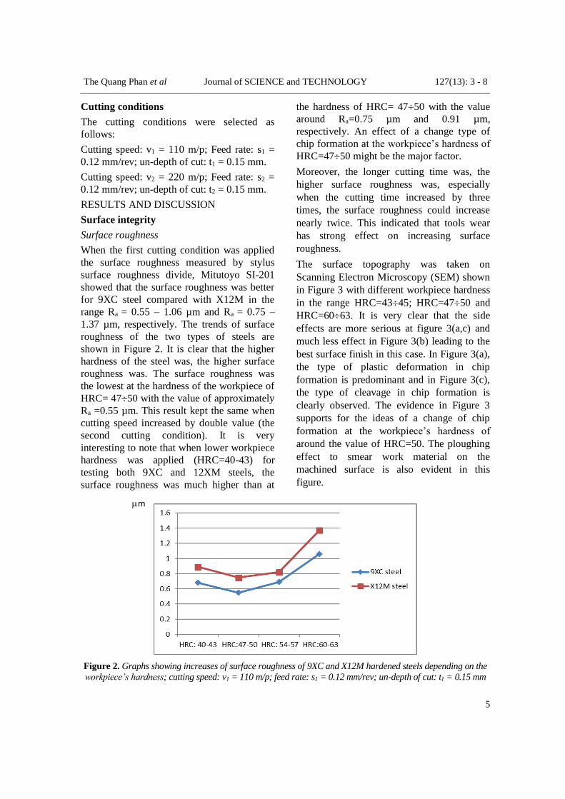
When the first cutting condition was applied
the surface roughness measured by stylus
surface roughness divide, Mitutoyo SI-201
showed that the surface roughness was better
for 9XC steel compared with X12M in the
range Ra = 0.55 – 1.06 µm and Ra = 0.75 –
1.37 µm, respectively. The trends of surface
roughness of the two types of steels are
shown in Figure 2. It is clear that the higher
hardness of the steel was, the higher surface
roughness was. The surface roughness was
the lowest at the hardness of the workpiece of
HRC= 4750 with the value of approximately
Ra =0.55 µm. This result kept the same when
cutting speed increased by double value (the
second cutting condition). It is very
interesting to note that when lower workpiece
hardness was applied (HRC=40-43) for
testing both 9XC and 12XM steels, the
surface roughness was much higher than at
the hardness of HRC= 4750 with the value
around Ra=0.75 µm and 0.91 µm,
respectively. An effect of a change type of
chip formation at the workpiece’s hardness of
HRC=4750 might be the major factor.
Moreover, the longer cutting time was, the
higher surface roughness was, especially
when the cutting time increased by three
times, the surface roughness could increase
nearly twice. This indicated that tools wear
has strong effect on increasing surface
roughness.
The surface topography was taken on
Scanning Electron Microscopy (SEM) shown
in Figure 3 with different workpiece hardness
in the range HRC=4345; HRC=4750 and
HRC=6063. It is very clear that the side
effects are more serious at figure 3(a,c) and
much less effect in Figure 3(b) leading to the
best surface finish in this case. In Figure 3(a),
the type of plastic deformation in chip
formation is predominant and in Figure 3(c),
the type of cleavage in chip formation is
clearly observed. The evidence in Figure 3
supports for the ideas of a change of chip
formation at the workpiece’s hardness of
around the value of HRC=50. The ploughing
effect to smear work material on the
machined surface is also evident in this
figure.
Figure 2. Graphs showing increases of surface roughness of 9XC and X12M hardened steels depending on the
workpiece’s hardness; cutting speed: v1 = 110 m/p; feed rate: s1 = 0.12 mm/rev; un-depth of cut: t1 = 0.15 mm
m

The Quang Phan et al Journal of SCIENCE and TECHNOLOGY 127(13): 3 - 8
6
Figure 3. SEM micrographs showing the surface topography after hard turning of X12M steel with
different hardness of workpiece: HRC=4345; HRC=4750 and HRC=6063; Cutting speed: v1 = 110
m/p; Feed rate: s1 = 0.12 mm/rev; un-depth of cut: t1 = 0.15 mm
The micro-hardness measurements on cross
section of the workpiece from the depth of 15
µm to 300 µm showed evidence the effects of
smearing on the machined surface resulting in
an increase in surface hardness at a very
narrow layer with the depth less than 15 µm.
It is reasonable because the depth of cut here
is quite small t = 0.15 mm at the level of
precision cutting and consistent with other
authors’ results.
Frictional Interactions between chip and rake face
It is evident in Figure 4(a) that at low
workpiece’s hardness (HRC=4345), the
length of contact is the longest (l = 300 µm)
and mainly covered by the work material.
However, the length of contact is reduced by
a half (l = 150 µm) shown in Figure 4(b)
when workpiece with the hardness of
HRC=5054 were machined. The rake face is
nearly free of material transfer. Moreover,
when the hardness of the workpiece was
HRC=6063, the length of contact increased
gain as shown in Figure 4(c) with l = 280 µm.
The main different compared with Figure 4(a)
is that material transfer is much less and
concentrated on the rear rake face. From
evidence in Figure 4, it is clear that there is a
change in frictional interactions between chip
and tool from mainly plastic type to cleavage
one in chip formation when the hardness of the
workpiece varied from around HRC=45 to 60.
Figure 4. SEM micrographs showing the rake face of PCBN inserts after hard turning of X12M steel with
different hardness of workpiece: HRC=4345; HRC=5054 and HRC=6063; Cutting speed: v1 = 110
m/p; Feed rate: s1 = 0.12 mm/rev; un-depth of cut: t1 = 0.15 mm
a) b) c)

The Quang Phan et al Journal of SCIENCE and TECHNOLOGY 127(13): 3 - 8
7
Discussion
From the results mentioned above in the study,
the best surface roughness (Ra = approximately
0.55 µm) was achieved when X12 and 9XC
steel with the hardness of HRC = around 50
was machined by the first and second cutting
conditions. With the hardness HRC = around
45 and higher than 55, the surface hardness
was much worse. The fact can be explained by
the change in chip formation from plastic type
toward cleavage type similar to machining
brittle materials as shown in Figure 4. This
also involves with the type of frictional
chip/rake face interactions. Short chip/rake
contact and free of material transfer results in
low surface roughness and better surface
topography. Long chip/rake face length of
contact and more material transfer in both near
the cutting edge and at the region where chip
breaks from contact with the rake face cause
the higher surface roughness and worse surface
topography. This is completely consistent with
the ideas that the length of chip/rake face
contact is directly proportional to the value of
cutting force and surface roughness as a result
of the level of adhesion between chip and tool.
The hardness of the workpiece could change
the frictional contact on the rake face. When
the hardness reached HRC=6063, the first
crater with short length of contact formed
near the cutting edge and then the second
crater appeared at the rear of the first crater.
The harder of the chip shortened the length of
chip/tool contact on the rake face and after a
while when the crater developed enough it
formed the second one due to the depth of the
first crater changed the frictional contact on
the rake face.
CONCLUSION
From this study, conclusions can be derived
as follows:
The surface integrity estimated by surface
roughness and surface topography is consider
to the best for both type of workpiece
materials at the hardness HRC= 4750. The
surface topography shows that at low
hardness of HRC = 4750 chip formation
mainly in plastic type and at high hardness of
HRC = 55 and above the chip formation
changed toward cleavage similar to brittle
materials in cutting.
The frictional chip/tool interactions are also
changed depending on the workpiece’s
hardness. The lower hardness the longer
chip/tool contact is with full of material
transfer on the contact area. However, when
the hardness of the workpiece is higher than
HRC = 55, the contact length is shortened
with free material transfer and after a duration
of cutting, the second crater appears at the
rear of the first crater with not much material
transfer.
REFERENCES
1. D.W. Schwach and Y.B. Guo.; “Feasibility of
producing optimal surface integrity by process
design in hard turning”, Materials Science and
Engineering, A 395 (2005), pp. 116-123.
2. Y.K. Chou., “Hard turning of M50 steel with
different microstructure in continuous and
intermittent cutting”, Wear 255 (2003), pp. 1388-
1394.
3. A. Barbacki, M. Kawalec, A. Hamrol.,
“Turning and Grinding as a source of of
microstructural changes in the surface layer of
hardened steel, Journal of Materials Processing
Technology, 133 (2003), pp. 21-25.
4. H.A. Kishawy and M.A. Elbestawi., “Effects
of process parameters on materials side flow
during hard turning”, International Journal of
Machine Tools & Manufacture, 39 (1999), pp.
1017-1030.
5. Y.K. Chou and C.J. Evans., “White layers and
thermal modeling of hard turned surfaces”,
International Journal of Machine Tools &
Manufacture, 39 (1999), pp. 1863 -1881.
6. N.T.Q. Dung., “A study of hard turning
process with the use of PCBN inserts”, PhD
Dissertation, Thai Nguyen University of
Technology, 2012.

The Quang Phan et al Journal of SCIENCE and TECHNOLOGY 127(13): 3 - 8
8
TÓM TẮT
ẢNH HƯỞNG CỦA ĐỘ CỨNG PHÔI
TRONG QUÁ TRÌNH TIỆN CỨNG THÉP HỢP KIM
Phan Quang Thế, Nguyễn Thị Quốc Dung*, Phan Thị Phương Thảo
Trường Đại học Kỹ thuật Công nghiệp – ĐH Thái Nguyên
Hiện nay, công nghệ tiện cứng đã được ứng dụng rộng rãi trong công nghiệp ở Việt Nam.
Tiện cứng thường là quá trình gia công lần cuối nên chất lượng bề mặt gia công đóng vai trò rất
quan trọng đối với việc sử dụng công nghệ tiện cứng trong hiện tại và tương lai. Bài báo này trình
bày kết quả một nghiên cứu về quá trình tiện cứng thép hợp kim 9XC và X12M nhằm xác định
ảnh hưởng của độ cứng phôi đến hình học và nhám bề mặt gia công trong điều kiện công nghệ xác
định. Kết quả cho thấy trong dải độ cứng từ 50 đến 60HRC nhám bề mặt tỉ lệ thuận với độ cứng
phôi. Tuy nhiện ở độ cứng thấp hơn chất lượng bề mặt giảm và nhám bề mặt tăng. Nhám bề mặt
đạt giá trị tốt ở độ cứng xấp xỉ 50HRC ngay cả khi tốc độ cắt tăng gấp đôi. Hiện tượng này được
cho là có liên quan đến việc thay đổi tương tác tiếp xúc giữa phôi và mặt trước của dao phụ thuộc
vào độ cứng phôi và mòn dụng cụ.
Từ khóa: Tiện cứng, nhám bề mặt, hình học, phôi, mòn dụng cụ.
* Tel: 0915308818; Email: [email protected]

Lanh Van Nguyen et al Journal of SCIENCE and TECHNOLOGY 127(13): 9 - 14
9
DIRECT MRAS BASED AN ADAPTIVE CONTROL SYSTEM FOR TWIN ROTOR MIMO SYSTEM
Lanh Van Nguyen*, Loc Bao Dam
University of Technology – TNU
ABSTRACT
In this paper, a Model Reference Adaptive Systems (MRAS) based an Adaptive System is
proposed to a Twin Rotor MIMO System (TRMS). The TRMS is an open-loop unstable, non-
linear and multi output system. The main task of this design is to keep the balance and to track a
given trajectory. There are two separate adaptive controllers designed for controlling two angles.
By applying Lyapunov stability theory the adaptive law that is derived in this study is quite simple
in its form, robust and converges quickly. Experimental results show that the proposed adaptive
PID controllers have better performance compared to the conventional PID controllers in the sense
of robustness against internal and/or external disturbances.
Index Terms – Model Reference Adaptive Systems (MRAS), Twin Rotor MIMO System (TRMS).
Keywords: Model Reference Adaptive Systems (MRAS), Twin Rotor MIMO System (TRMS).
INTRODUCTION*
The TRMS which isa model of the simpli fied
heli copter. Its position and velo city are
controlled by changing the speed of pitch and
yaw rotors. The TRMS system has high non
line arity, uncer tainty, especially coupling
between input sandout puts. This would be
avery complicated problem if we want to
control the TRMS moving quickly and
accurately to the desired location or a given
trajectory. The motion control system can
bequite complex because many different
factors must be conside redin the design. It's
hard to figure out the design methods that
consider all the factors such as: reducethe
effects of noise, object variable parameters,
avoid the influence of the coupling. There is
nosing lesolution to this problem.
There have been many research papers in
order to control the system. How ever the
classic controller will notachieve the desire
dresults. There fore, advanced controller was
introduced.
In this study, design of MRAS-based adaptive
control systems is developed for the TRMS
which acts on the errors to reject system
* Tel: 0974161383; Email: [email protected]
disturbances, and to cope with system
parameter changes. In the model reference
adaptive systems the desired closed loop
response is specified through a stable
reference model. The control system attempts
to make the process output similar to the
reference model output.
Fig 1: Experimental setup
Figure 1. Experimental setup
The proposed controller is expected to
improve the tracking performance and
increase the robustness under the effects of
disturbances and parameter changes. Two
separate adaptive controllers are designed
based on the Lyapunov’s stability theory for
controlling two given trajectory.
This paper is organized as follows. Design of
MRAS based an adaptive controller is

Lanh Van Nguyen et al Journal of SCIENCE and TECHNOLOGY 127(13): 9 - 14
10
introduced in Section II. In Section III, the
dynamics of the twin rotor MIMO system is
shown. The design of the proposed controller
is introduced in Section IV. The experimental
results are also presented in section V. At the
end of this paper, summary of the paper is
given.
DESIGN OF DIRECT MRAS
Figure 2. Adaptive system designed with Liapunov
The structure depicted in Fig 1 can be used as
an adaptive PID controlled system. A second-
order process is controlled with the aid of a
PID-controller. Variations in the process
parameters bp, ap and Kw can be compensated
for by variations in parameters of this
controller Kp, Kd and Ki. We are going to find
the form of the adjustment laws for Kp, Kd and
Ki. The following steps are thus necessary to
design an adaptive controller with the method
of Lyapunov:
1. Determine the differential equation for :
= , (1) where and are
states of the reference model and process,
respectively.
2. Choose a Lyapunov function :
= , (2) in which a positive
definite symmetrical matrix, a diagonal
matrix with in principle arbitrary coefficients
0, and is the parameter error vector.
3. Determine the condition under which is
definite negative.
4. Solve from , (3)
where is the process matrix and is a
positive definite symmetrical matrix. This
yields, the form of the adjustment laws [2]:
(4)
In Equation 4 , and are called the
adaptive gains, and , , , , and are
defined in Fig 2, , are elements of the
matrix.
TWIN ROTOR MIMO SYSTEM
In order to design a controller for the TRMS,
a dynamical model is first required [3].
DESIGN OF CONTROL SYSTEM
PID Control System with Fixed Parameters

Lanh Van Nguyen et al Journal of SCIENCE and TECHNOLOGY 127(13): 9 - 14
11
The PID control algorithm is mostly used in
the industrial applications since it is simple
and easy to implement when the system
dynamics is not available. For the TRMS
control variables are a pitch angle and yaw
angle such that two separate controllers
are required. In this study, the PID controller
is used for the given trajectories control.
There are many methods of choosing suitable
values of the three gains to achieve the
satisfied system performance. In this study,
the Ziegler – Nichols approach is used to
design PID controller to achieve a desired
system performance.
+
+
Twin Rotor
MIMO
System
-
PID1
PID2
-
Fig 3: PID controller structure
Figure 3. PID controller structure
Adaptive PID Control System
For purposes of comparison, the process is
repeated using an adaptive control structure.
The pitch angle and yaw angle of the TRMS
are controlled separately by two adaptive
controllers by replacing two corresponding
linear controllers indicated in Fig. 4.
Reference Model
Reference model is described by the transfer
function:
(6)
The parameters of the reference model are
chosen such that the higher order dynamics of
the system will not be excited. This leads to
the choice of
and , such that:
(7)

Lanh Van Nguyen et al Journal of SCIENCE and TECHNOLOGY 127(13): 9 - 14
12
Figure 4. Adaptive PID control structure
State Variable Filter
As mentioned in Section II, the derivative of
the error can be created using a state variable
filter. The parameters of this state variable
filter are chosen in such a way that the
parameters of the reference model can vary
without the need to change the parameters of
the state variable filter every time. The
parameters are chosen as:
, and , then
(8)
Adaptive Controllers based on MRAS
Follow Ep. (4) the complete adaptive laws in
integral form for the pitch angle controller are
(9)
For the yaw controller
(10)
In the form of the adjustment laws ,
, and are elements of the
and matrices, obtained from the solution of
the Lyapunov equations indicated in Eq. (11):
;
(11)
- + +
- +
Reference Model 2
- +
+ -
+ + +
- Lyapunov
SVF
SVF
+ -
- +
Reference Model 1
- +
+ + -
Twin Rotor MIMO System
+ + +
-
-
-
+ +
Lyapunov
+ +

Lanh Van Nguyen et al Journal of SCIENCE and TECHNOLOGY 127(13): 9 - 14
13
where and are positive definite
matrices and and are:
(12)
With , ;
and are adaptive
gains.
EXPERMENTAL TESTS
From the experimental results with two sets
of PID controller and adaptive PID controller
in Fig 5 we find that, the system using
adaptive PID controller has result in sticking
and eliminates noise better than that useing
the classical PID one.
Figure 5. Responses of the PID control system (left hand side)and adaptive PID control (right hand side)
system with disturbance
Fig 6. Adaptive PID parameter

Lanh Van Nguyen et al Journal of SCIENCE and TECHNOLOGY 127(13): 9 - 14
14
CONCLUSION
In this paper, the conventional PID controller
and the adaptive PID controllers are
successfully designed to TRMS under
disturbances. The simple adaptive control
schemes based on Model Reference Adaptive
Systems (MRAS) algorithm are developed for
the asymptotic output tracking problem with
changing system parameters and disturbances
under guaranteeing stability. Experiments
have been carried out to investigate the effect
of changing the external disturbance forces on
the system. Based on the experimental results
and the analysis, a conclusion has been made
that both conventional and adaptive
controllers are capable of controlling the
given trajectory of the non-linear system.
However, the adaptive PID controller has
better performance compared to the
conventional PID controller in the sense of
robustness against disturbances.
REFERENCE
1. Van Amerongen, J., Intelligent Control (part
1)-MRAS, Lecture notes, University of Twente,
The Netherlands, March 2004.
2. Nguyen Duy Cuong, Nguyen Van Lanh, Dang
Van Huyen, “Design of MRAS-based Adaptive
Control Systems”, The IEEE 2013 International
Conference on Control, Automation and
Information Sciences (ICCAIS), pp. 79 - 84, 2013.
3. Twin Roto MIMO System Control
Experiments 33-949S Feedback Instruments Ltd,
East susex, U.K., 2006.
TÓM TẮT
HỆ THỐNG THÍCH NGHI MÔ HÌNH MẪU TRỰC TIẾP DỰATRÊN HỆ THỐNG ĐIỀU KHIỂN THÍCH NGHI CHO HỆ THỐNG TWIN ROTOR MOMO
Nguyễn Văn Lanh*, Đàm Bảo Lộc
Trường Đại học Kỹ thuật Công nghiệp – ĐH Thái Nguyên Bài báo này, đề xuất một hệ thống thích nghi theo mô hình mẫu (MRAS) đã được áp dụng vào hệ
thống Twin Rotor MIMO (TRMS). TRMS là một hệ thống hở không ổn định, phi tuyến có nhiều
đầu vào/ra. Mục đích chính của thiết kế này nhằm giữ cho hệ thống cân bằng và chuyển động bám
theo một quỹ đạo cho trước. Để thực hiện thiết kế cần thực hiện qua các bước sau: Bước 1, xây
dựng hệ phương trình chuyển động của đối tượng dựa theo phương trình Lagrange. Bước 2, thực
hiện tuyến tính hóa các phương trình. Bước 3, thiết kế hai bộ điều khiển thích nghi độc lập để điều
khiển hai góc đầu ra. Luật điều khiển thích nghi áp dụng lý thuyết ổn định Lyapunov có dạng đơn
giản, bền vững và hội tụ nhanh. Các kết quả mô phỏng và thực nghiệm chỉ ra rằng các bộ điều
khiển PID thích nghi có chất lượng tốt hơn khi so sánh với các bộ điều khiển PID thông thường
dưới tác động của các nhiễu bên trong và/ hoặc nhiễu ngoài.
Từ khóa: Hệ thống thích nghi theo mô hình mẫu (MRAS), Hệ nhiều đầu vào nhiều
đầu ra Twin Rotor (TRMS).
* Tel: 0974161383; Email: [email protected]

Minh Y Nguyen et al Journal of SCIENCE and TECHNOLOGY 127(13): 15 - 20
15
A NEW APPROACH FOR ENERY SAVING TO HOUSEHOLD CUSTOMERS BASED SMARTGRID TECHNOLOGIES
Minh Y Nguyen*, Thang N. Pham and Toan H. Nguyen
University of Technology – TNU
ABSTRACT
This paper addresses the energy efficiency problem of household customers by observing and
responding accordingly to the condition of the upstream grid; the key condition is the market price
which is passed to the end-use customers though a new market entity, namely load aggregators. A
framework based on Smargrid technologies, e.g., Advanced Metering Infrastructure (AMI) for
monitoring home energy consumptions is proposed. The problem is to schedule and control the
home electrical appliances in response to the market price to minimize the energy cost over a day.
The problem is formulated using Dynamic Programming (DP) and solved by DP backward
algorithm. Using stochastic optimization techniques, the proposed framework is capable of
addressing the uncertainties related to the appliance performance: outside temperature and/or
users’ habits, etc.
Keywords: Demand response, Home energy efficiency, Heat ventilation and air conditioning,
Dynamic programming, Smartgrid.
INTRODUCTION*
This paper discusses a new approach to
energy efficiency in the residential sector by
watching the household consumption from
the system perspective: it is more economical
and efficient not only for household
customers but the system-wide if the
appliances and lighting are turned on in low
price times and off in the high time. This can
be referred to as Demand Response (DR)
program and/or Home Energy Management
System (HEMS). Herein, we propose a DR
framework for a household that consists of
two functions: (1) Off-line scheduling
according to the prediction and (2) On-line
control based on both the previous scheduling
and real-time load measurements. The
framework is based on advanced
communication and automation technologies
applied to the power grid, i.e., Smartgrid with
the key component is Advanced Metering
Infrastructure (AMI). The problem is finding
out the optimal consumption each time slot
* Tel: 0966996399; Email: [email protected]
(stage) of the day to minimize the overall
energy cost, subject to the constraint of the
physical system and the users’ preference of
comfort.
THE PROPOSED DEMAND RESPONSE
FRAMEWORK
The proposed DR framework for household
customers is sketched in Fig. 1. As
aforementioned, under market environments
electric customers are offered choices to pay
their usage corresponding to the condition of
the wholesale market, i.e., real-time price.
The matter of fact is that it is not suitable for
human to analyze and respond to the frequent
change over time of the real-time price (e.g.,
every 5 min.). Therefore, advanced
communication and automations, also known
as Smartgrid technologies are essentially
needed here. The proposed scheme consists of
two different functions: (1) Off-line
scheduling according to the anticipated price
and load models and (2) On-line control
combining both the scheduling ahead and the
real-time measurements.

Minh Y Nguyen et al Journal of SCIENCE and TECHNOLOGY 127(13): 15 - 20
16
Figure 1. The DR framework based on AMI for household customers
Day-ahead Scheduling
The problem of day-ahead scheduling is to
find out the so-called “control policy” that
minimizes the expected energy cost over a
day with respect to the uncertainties of the
forecasting. The solution is subject the
constraints associated the physical system
capacity and/or the users’ preference of
comfort, etc. It is worth noting that the
decision is made in accordance with the time
basis of the electricity market, which is 5 min.
in this paper. The problem can be formulated
as follows [7].
1
0 0,1... 1 0,1... 1
min , ,k k
N
N N k k k kku wk N k N
E g x g x u w
(1)
Subject to
1 , , , 0,1... 1k k k k kx f x u w k N (2)
min max , 0,1... 1ku u u k N (3)
min max , 1, 2...kx x x k N (4)
1,2...
, , 0, 1,2...i k k k k Nh x u w i n
(5)
where xk the state variable at the beginning of
stage k; uk the control variable during stage k;
wk the uncertainty during stage k; N is the
number of stages over the scheduling period;
gN(xN) is the terminal cost, i.e., the cost
associated with the final state; gk(xk,uk,wk) is
the cost in stage k; fk(xk,uk,wk) is the state
transition function; umin, umax are the capacity
limits; xmin, xmax are the physical limits of the
system; and hi(x1,x2…xN) refers to the
customers’ preference, e.g., human would feel
comfortable if the temperature is kept within
22–260C with HVAC; batteries must be full
of charge by 7:00 AM (i.e., the time to go
working) with EVs.
In this formulation, equation (1) is the
objective function, i.e., minimizing the energy
costs over a day subject to the uncertainties.
Equation (2) shows the modeling of loads
which represents the dynamics (state
transition) of the load performance. Equations
(3) and (4) are the physical constraint of the
loads. Finally, equation (5) represents the
conditions to be comfortable setup by
customers and n is the number of functions
needed.
Figure 2. The proposed DR framework and its
variables defined in stage k

Minh Y Nguyen et al Journal of SCIENCE and TECHNOLOGY 127(13): 15 - 20
17
The control policy resulted from the day-
ahead scheduling is a set of functions of the
system state, denotes μk(xk), k = 0, 1…N-1,
that will point out the optimal control of the
system provided the measurement of the
current state (i.e., the scenario is cleared).
Real-time Controller
The fact is that the scenario probably differs
from the anticipation due to many uncertain
factors, e.g., weather, temperature and users’
demands, etc. Therefore, the real-time control
should not only follow the previous schedule
but also depend on the real-time measurement
of the system. With the control policy
determined ahead of time, the decision in
real-time operation can be made as simply as:
*
k k ku x (6)
where xk is measures of the state variable.
The block diagram of the proposed DR and its
variables defined in stage k are expressed in
Fig. 2.
ILLUSTRATIVE EXAMPLE
This section provides an illustrative example
where the proposed framework is tested in the
DR problem of HVAC loads in a real-time
electricity market. The idea of HVAC is
taking advantages of the slow dynamics of the
heating/cooling process compared to the
changing rate of the price signal (i.e., 5 min.)
to manage the HVAC operation with the
target of minimizing the total energy cost in a
day while maintain comfort levels to the
users. The framework specified for HVAC is
as follows.
1
0 0,1... 10,1... 1
min ac
kk
N ac
k kkTqk Nk N
E q
(7)
Subject to
1
1
or
1 , 0,1... 1
ac
k k k k k
ac
k k k k
t t q T t
t t q T k N
(8)
min max , 0,1... 1ac ac ac
kq q q k N (9)
min max , 1,2...kt t t k N (10)
whereac
kq is the energy consumption of
HVAC during state k, [kWh]; tk is the indoor
temperature at the beginning of stage k, [0C];
Tk is the outside average temperature during
stage k, [0C]; N is the number of stages; α is
the equivalent thermal resistance of HVAC,
[0C/kWh]; β is the coefficient of the heat
transfer between the indoor and outdoor
space, [p.u.]; min max,ac acq q are the capacity limits
of HVAC, [kWh]; and tmin, tmax are the lower
and upper temperature of human comforts,
[0C], e.g. human feels comfortable with the
temperature between 22–260C. It is worth
noting that with time basis of electricity
market is 5 min., resulting in the number of
stages is 24×12 = 288 in a day. The control policy constructed through the above scheduling problem combined with the real-time measurements (of the actual indoor temperature) will be used to determine the optimal decision as follows.
*
k k kq t (11)
The proposed HVAC scheme will be compared with the traditional scheme that HVAC is controlled by a thermostat. With the upper/lower set-points, HVAC will be switched on/off when the indoor temperature reaches the lower or upper bound of the customers’ preference, respectively. This can be described mathematically in the following.
max min
1 min max
max
if
if
0 if
ac
k
ac ac
k k k
k
q t t
q q t t t
t t
(12)
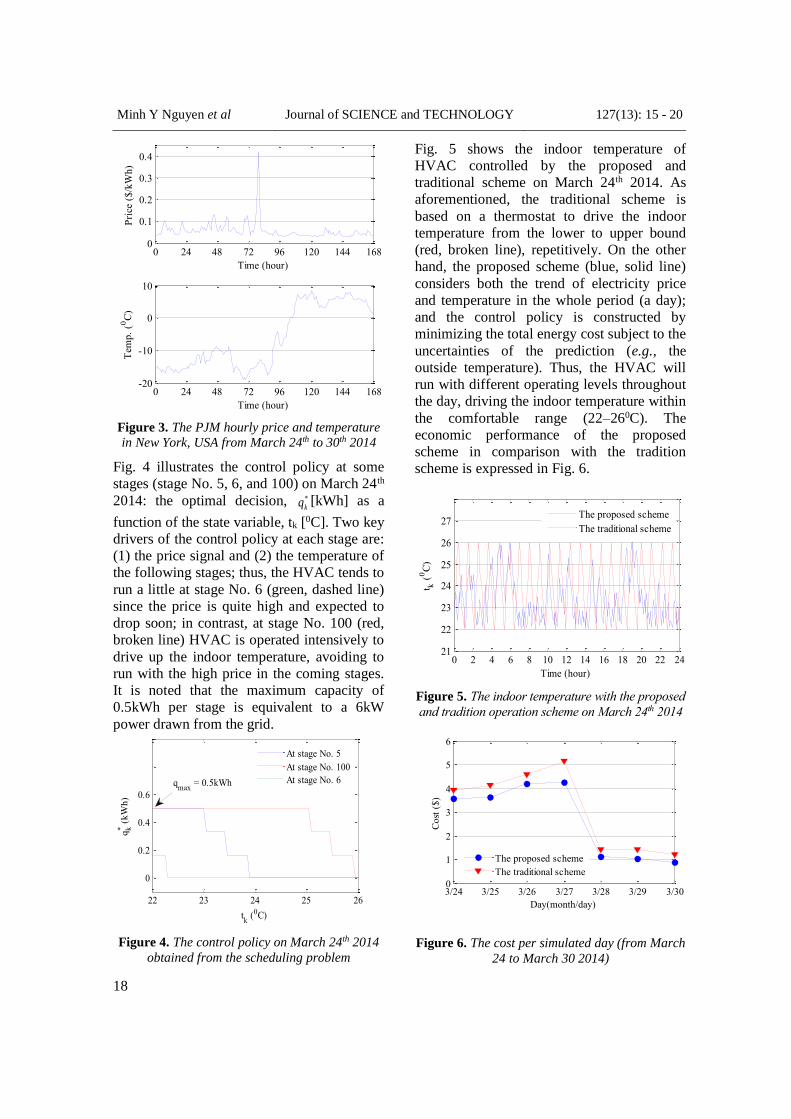
The price data used in this study is obtained by modifying the hourly electricity price of PJM market from March 24th to 30th 2014 (Monday to Sunday of a whole week) [8]. It is noted that the hourly price is determined through day-ahead bidding in electricity markets. The real-time imbalance caused by load deviations from the anticipation will be handled by calling upon the up/down regulation services; this action results in the real-time price differed from the hourly price [9]. The temperature in this study is referred from National Climate Data Center at New York, USA in the same period as the PJM price [10]. The price and temperature data are displayed in Fig. 3.
Minh Y Nguyen et al Journal of SCIENCE and TECHNOLOGY 127(13): 15 - 20
18
0 24 48 72 96 120 144 1680
0.1
0.2
0.3
0.4
Time (hour)
Pri
ce (
$/k
Wh
)
0 24 48 72 96 120 144 168-20
-10
0
10
Time (hour)
Tem
p.
(0C
)
Figure 3. The PJM hourly price and temperature
in New York, USA from March 24th to 30th 2014
Fig. 4 illustrates the control policy at some
stages (stage No. 5, 6, and 100) on March 24th
2014: the optimal decision, *
kq [kWh] as a
function of the state variable, tk [0C]. Two key
drivers of the control policy at each stage are:
(1) the price signal and (2) the temperature of
the following stages; thus, the HVAC tends to
run a little at stage No. 6 (green, dashed line)
since the price is quite high and expected to
drop soon; in contrast, at stage No. 100 (red,
broken line) HVAC is operated intensively to
drive up the indoor temperature, avoiding to
run with the high price in the coming stages.
It is noted that the maximum capacity of
0.5kWh per stage is equivalent to a 6kW
power drawn from the grid.
22 23 24 25 26
0
0.2
0.4
0.6
tk (0C)
q* k (
kW
h)
At stage No. 5
At stage No. 100
At stage No. 6qmax
= 0.5kWh
Figure 4. The control policy on March 24th 2014
obtained from the scheduling problem
Fig. 5 shows the indoor temperature of
HVAC controlled by the proposed and
traditional scheme on March 24th 2014. As
aforementioned, the traditional scheme is
based on a thermostat to drive the indoor
temperature from the lower to upper bound
(red, broken line), repetitively. On the other
hand, the proposed scheme (blue, solid line)
considers both the trend of electricity price
and temperature in the whole period (a day);
and the control policy is constructed by
minimizing the total energy cost subject to the
uncertainties of the prediction (e.g., the
outside temperature). Thus, the HVAC will
run with different operating levels throughout
the day, driving the indoor temperature within
the comfortable range (22–260C). The
economic performance of the proposed
scheme in comparison with the tradition
scheme is expressed in Fig. 6.
0 2 4 6 8 10 12 14 16 18 20 22 2421
22
23
24
25
26
27
Time (hour)
t k (
0C
)
The proposed scheme
The traditional scheme
Figure 5. The indoor temperature with the proposed
and tradition operation scheme on March 24th 2014
3/24 3/25 3/26 3/27 3/28 3/29 3/300
1
2
3
4
5
6
Day(month/day)
Co
st (
$)
The proposed scheme
The traditional scheme
Figure 6. The cost per simulated day (from March
24 to March 30 2014)

Minh Y Nguyen et al Journal of SCIENCE and TECHNOLOGY 127(13): 15 - 20
19
Fig. 6 shows the energy cost in each day of
the simulated period: from March 24th to 30th
2014. Generally, the cost is quite high from
March 24th to 27th due to two reasons: first,
the weather is cold with the temperature is
usually lower than –10 Degree Celsius and
secondly, the electricity price is relative high
in weekdays (from Monday to Thursday),
particularly the critical peak price occurs on
Thursday March 27th. In contrast, the cost
from March 28th to 30th is much slower
because the temperature rises significantly
(0–10 Degree Celsius) and the electricity
price also decreases somehow in the
weekend.
As the simulation results, it can be recognized
that significant saving can be obtained by the
proposed DR scheme on HVAC loads
compared to the traditional operation.
Particularly with the critical peak price on
Thursday, the proposed scheme can manage
the energy cost to be not increased that much
and obtain the highest saving throughout the
simulated week. In overall, the energy cost
with the proposed scheme is 18.67$ while that
with the traditional scheme is 21.85$; the
saving in this case is about 14.55%. The
HVAC modeling parameters and the
customer preference is provided in Table 1.
Table 1. The parameters used in the simulation of
the illustrative example
System
parameters
Customer
preferences
α (0C/kWh) 2.5 tmin (0C) 22
β (p.u.) 0.015 tmax (0C) 26
min
hvacq (kWh) 0
max
hvacq (kWh) 50
CONCLUSION
This paper has presented a new framework
for the energy efficiency of household
customer based on Smartgrid technologies
applied into the existing power grid. The
saving can be achieved by customers actively
responding to the market price which is
passed to the end-users though load
aggregators. The proposed framework is
comprised of two main functions: (1) Off-line
scheduling according to the anticipated data
and (2) On-line control based on both the
ahead scheduling and the real-time
measurements. The problem is formulated
and solved by DP backward algorithm, i.e.,
minimizing the expected energy cost over a
day subject to the uncertainty of the
forecasting. The proposed framework has
been specified and tested in HVAC loads
under real-time electricity. The electricity
price is referred from the PJM electricity
market and the temperature is from National
Climate Data Center in New York, USA in
the same period: from March 24th to 30th 2014
(the whole week). The simulation results
showed that the proposed scheme is not only
capable of controlling the indoor temperature
within the comfortable range (22–260C) set
by customers but the energy costs can be
saved remarkably. The amount of saving over
the simulated period compared with the
traditional operation scheme is as high as
14.55% in this study.

Minh Y Nguyen et al Journal of SCIENCE and TECHNOLOGY 127(13): 15 - 20
20
REFERENCES
1. A. Brooks, E. Lu, D. Reicher, C. Spirakis and
B. Weihl, “Demand dispatch: Using real-time
control of demand to help balance generation and
load,” IEEE Power and Energy Magazine (2010).
Vol. 5, No. 3, pp. 20-29.
2. S. Majumdar, D. Chattopadhyay and J. Parikh,
“Interruptible load management using optimal
power flow analysis,” IEEE Trans. Power Systems
(1996) Vol. 11, No. 2, pp. 715-720.
3. M.A. Pedrasa, T. D. Spooner and I. F.
MacGill, “Scheduling of demand side resources
using binary particle swarm optimization,” IEEE
Trans. Power Systems (2009), Vol. 24, No. 3, pp.
1173-1181.
4. Z. Fan, “A distributed demand response
algorithm and its application to PHEV charging in
smart grid,” IEEE Trans. Smart Grid (2012), Vol.
3, No. 3, pp. 1280-1291.
5. T. M. Calloway and C. W. Brice, “Physically
based model of demand with applications to load
management assessment and load forecasting,”
IEEE Trans. Power Systems, PAS Vol. 101,
No.12, pp. 4625-4631.
6. J. H. Yoon, R. Baldich and A.Novoselac,
“Dynamic demand response controller based on
real-time retail price for residential buildings,”
IEEE Trans. Smart Grid (2014), Vol. 5, No. 1, pp.
121-129.
7. D. P. Bertsekas, Dynamic Programming and
Optimal Control. Athena Scientific: Belmont,
MA, USA, 1995.
8. PJM Electricity market. Available online:
http://www.pjm.com (accessed on 1st April 2014.)
9. M. Y. Nguyen, V. T. Nguyen, and Y. T. Yoon,
“A new battery energy storage charging/
discharging scheme for wind power producers in
real-time markets,” Energies (2012), Vol. 5, No.
12, pp. 5439-5452.
10. National Climate Data Center (NCDC).
Available online: HTTP://NCDC.NOAA.GOV
(accessed on 1st April 2014).
TÓM TẮT MỘT PHƯƠNG PHÁP TIẾP CẬN MỚI CHO VIỆC TIẾT KIỆM ĐIỆN NĂNG CHO CÁC HỘ TIÊU THỤ DỰA TRÊN CÔNG NGHỆ SMARTGRID
Nguyễn Minh Ý*, Phạm Ngọc Thăng và Nguyễn Huy Toán
Trường Đại học Kỹ thuật Công nghiệp – ĐH Thái Nguyên
Bài báo đề cập đến vấn đề nâng cao hiệu quả trong việc sử dụng điện năng tại các hộ tiêu thụ điện
bằng cách dự báo, cập nhật và xử lý các thông tin về lưới điện; trong thị trường điện, các thông tin
này được phản ánh thông qua giá điện và được truyền đến người dung điện theo thời gian thực
thông qua các công ty bán điện. Trên cơ sở đó, bài báo đề xuất một mô hình quản lý và điều khiển
các thiết bị điện trong hộ gia đình dựa trên những công nghệ của mạng điện thông minh
(Smartgrid) với hàm mục tiêu là tối giảm hóa chi phí tiêu thụ điện năng trong ngày. Bài toán được
mô hình bằng phương pháp quy hoạch động (Dynamic programming) và giải bằng thuật toán tính
ngược (Backward algorithm). Ứng dụng lý thuyết sắc xuất thống kê, các đại lượng ngẫu nhiên như
nhiệt độ môi trường hay nhu của cầu người sử dụng cũng sẽ được giải quyết.
Từ khóa: Điều khiển phụ tải, hiệu suất sử dụng năng lượng, hệ thống điều hòa trung tâm, quy
hoạch động, mạng điện thông minh.
* Tel: 0966996399; Email: [email protected]
Dinh Thi Gia et al Journal of SCIENCE and TECHNOLOGY 127(13): 21 - 28
21
DIRECT MRAS WITH SAFE CONSTRAINTS APPLIED FOR TWO-WHEELED MOBILE ROBOT
Dinh Thi Gia, Tuan Manh Tran, Son Que Tran*
University of Technology – TNU
ABSTRACT
Most two-wheeled mobile robots (TWMR) are controlled and moved by two DC motors. The
heading angular velocity depends on the changing velocity of two wheels mounted on the two DC
motors respectively. During moving, if the heading angular velocity and the linear velocity are too
high, it can lead to flip and slide phenomena. In addition, under the effects of noises (internal and
external), TWMR may be unstable. To solve these problems, we use Euler-Lagrange method to
model for TWMR, build safe conditions against flip, then apply the Model Reference Adaptive
System (MRAS) to construct an adaptive controller for TWMR to ensure the required motion,
stability and safety. Simulation results and analysis point out the effectiveness of the designed
controller.
Keywords: Direct MRAS, Two wheeled mobile robot.
INTRODUCTION *
Two-wheeled mobile robot is shown in Fig. 1
including two wheels, a chassis and a
pendulum. In fact, TWMR - a nonlinear,
unstable and underactuated system - is built
based on the principle of the inverted
pendulum dynamics. To model TWMR, two
widely used methods are Newton and Euler-
Lagrange [1]. With this configuration, It has
been considered as anuseful prototype for
representing nonlinear systems when testing
control algorithms.
To design control for TWMR, the moments
which put into two wheels to control
movement and stability are computed.
When designing controller, the following
parameters are interested: the title angle is
stable at the reference and there is no
overturn while TWMR moving. Although
the system is unstable, difficult to control,
the TWMR is usually used because of the
ability to move in tight space, various terrain
and sharp corners [2].
After linearization, ignoring nonlinear,
coupling attributes, the linear algorithms as
PID, MRAS, etc are applied because they are
* Tel: 0988039336; Email: [email protected]
quite simple, quick converge, and have small
area stability. On the other hand, the
nonlinear algorithms are complexity, huge
computation, and long response time, but they
have the larger area of stability. However,
under the effect of disturbance, most
conventional controllers can not warrant the
robust performance of system. Normally,
adaptive controller would be the best choice
for this case. It can be easily seen that when
TWMR is drived by human, the TWMR is
affected by unknown forces or disturbance.
This domination is one first daresay in safe
control. The second task must be concerned
that the suitable controller must guarantee that
there are no overturn happening with human
and TWMR. It is quite scarce to find a
controller solving with human safety accept
for author in [2]. In this publication, the
author used a reduced-order disturbance
observer to estimate the disturbance acting on
the TWMR. This estimates disturbance and
compensates in the controller to reduce the
error signal.
In this paper, the model of TWMR is
expanded to three dimensions by using
unequal torque acting on each wheel of
TWMR. It clearly seen that TWMR will

Dinh Thi Gia et al Journal of SCIENCE and TECHNOLOGY 127(13): 21 - 28
22
rotate itself around z-axis. We continue use
the direct MRAS method designing control
for TWMR to reject system disturbances and
interest to the human safety issues. Two main
issues affecting human feeling are vibrations
when driving under disturbances and safety
when turning with high rotational speed. The
details are presented in Section IV. The
organization of this paper is as follows: After
Section I, introduction, Section II presents the
dynamics of TWMR based on Lagrange
method. In Section III, some basic steps for
designing an adaptive controller based on
direct Model Reference Adaptive System
(MRAS) are presented. Section IV is
mentioned above. In this Section, a MRAS
controller to stabilize position, velocity and
some simulation results are shown. Summary
of this paper is expressed in Section V.
TWO-WHEELED MOBILE ROBOT
In order to design a controller for TWMR, a
dynamic model is first considered. The
equations of motion of TWMR are
established based on balancing forces and
moments on the left wheel, right wheel, the
chassis, and the pendulum. A diagram of
forces and moments acting on the TWMR is
shown in Fig. 1. Definition of parameters and
variables of the TWMR is given in Table 1.
Figure 1. TWMR parameters
Table 1. TWMR parameters and variables
FL, FR Interacting forces between the left
and right wheels and the chassis
HL, HR Friction forces acting on the left and
right wheels
TL, TR Torques provided by wheel actuators
acting on the left and right wheels
fdL, fdR External forces acting on the left and
right wheels
Td External torque acting on the
pendulum
L, R Rotational angles of the left and right
wheels
xL, xR Displacements of the left and right
wheels along the x-axis
Tilt angle of the pendulum
Heading angle of the vehicle
x Displacement of the vehicle along the
x-axis
Mw Mass of the wheel
Jw Moment of inertia of the wheel with
respect to the y-axis
R Radius of the wheel
M Mass of the pendulum
G Gravity acceleration
L Distance from the point O to the
center of gravity, CG, of the
pendulum
D Distance between the left and right
wheels along the y-axis
M Mass of the chassis
Jc Moment of inertia of the chassis
about the y-axis
Jv Moment of inertia of the chassis and
pendulum about the z-axis
Lx , Rx and are chosen as generalized
coordinates. Calculating the kinetic energy for
each component, the final nonlinear dynamics
of TWMR are given as following
2 2
0
2
0
2
0
2
0
( )
sin( )
(
sin( )
sin( )(1)
)sin(
( )
2
)
L RdR dL
x
L RdR dL d
L RdL dR
gm l
J T Tm f f
R R
cosx
l
l cos
l
M mgl m
m T Tf f T
co
R R
D T Tf f
J R
s
R
(1)
Dinh Thi Gia et al Journal of SCIENCE and TECHNOLOGY 127(13): 21 - 28
23
where
2
ww 22
v
D JJ M J
R
; 2
p cJ m J Jl ;
ww 2
2x
JM M M m
R
2
ww 22
v
D JJ M J
R
; 2
0
2 2 ( )x l cosM J m
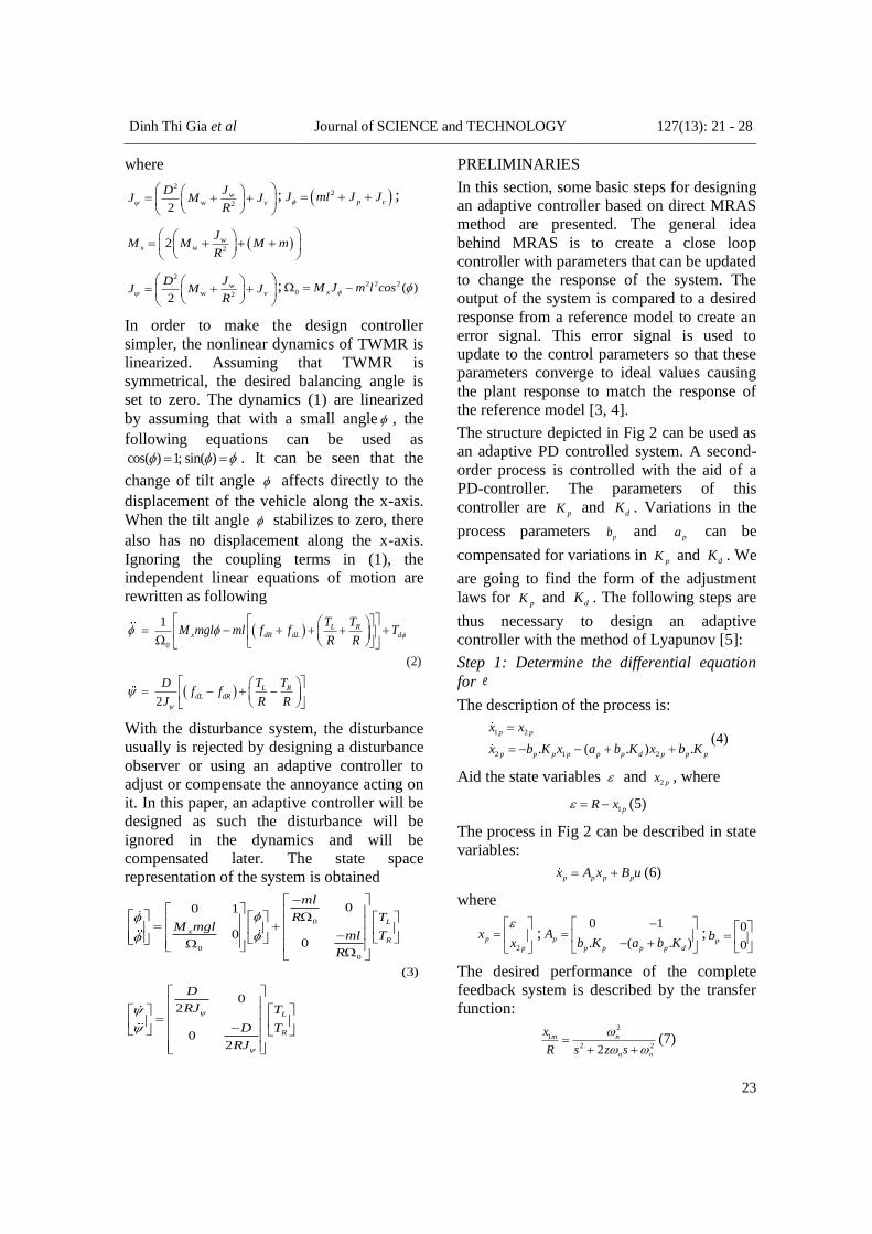
In order to make the design controller
simpler, the nonlinear dynamics of TWMR is
linearized. Assuming that TWMR is
symmetrical, the desired balancing angle is
set to zero. The dynamics (1) are linearized
by assuming that with a small angle , the
following equations can be used as
cos( ) 1; sin( ) . It can be seen that the
change of tilt angle affects directly to the
displacement of the vehicle along the x-axis.
When the tilt angle stabilizes to zero, there
also has no displacement along the x-axis.
Ignoring the coupling terms in (1), the
independent linear equations of motion are
rewritten as following
0
1
(2)
2
L Rx dR dL d
L RdL dR
T TM mgl m f f T
R R
D T Tf f
J R R
l
With the disturbance system, the disturbance
usually is rejected by designing a disturbance
observer or using an adaptive controller to
adjust or compensate the annoyance acting on
it. In this paper, an adaptive controller will be
designed as such the disturbance will be
ignored in the dynamics and will be
compensated later. The state space
representation of the system is obtained
0
0
0
00 1
00
(3)
02
02
L
x
R
L
R
ml
R TM mgl
ml T
R
D
RJ T
D T
RJ
PRELIMINARIES
In this section, some basic steps for designing
an adaptive controller based on direct MRAS
method are presented. The general idea
behind MRAS is to create a close loop
controller with parameters that can be updated
to change the response of the system. The
output of the system is compared to a desired
response from a reference model to create an
error signal. This error signal is used to
update to the control parameters so that these
parameters converge to ideal values causing
the plant response to match the response of
the reference model [3, 4].
The structure depicted in Fig 2 can be used as
an adaptive PD controlled system. A second-
order process is controlled with the aid of a
PD-controller. The parameters of this
controller are pK and dK . Variations in the
process parameters pb and pa can be
compensated for variations in pK and dK . We
are going to find the form of the adjustment
laws for pK and dK . The following steps are
thus necessary to design an adaptive
controller with the method of Lyapunov [5]:
Step 1: Determine the differential equation
for e
The description of the process is:
1 2
2 1 2. ( . ) .
p p
p p p p p p d p p p
x x
x b K x a b K x b K
(4)
Aid the state variables and 2 px , where
1pR x (5)
The process in Fig 2 can be described in state
variables:
p p p px A x B u (6)
where
2
p
p
xx
;0 1
. ( . )p
p p p p d
Ab K a b K
;
0
0pb
The desired performance of the complete
feedback system is described by the transfer
function: 2
1
2 22
m n
n n
x
R s z s
(7)

Dinh Thi Gia et al Journal of SCIENCE and TECHNOLOGY 127(13): 21 - 28
24
By the same way, the description of the
reference model is:
m m m mx A x B u (8)
where
2
m
m
m
xx
;2
0 1
2m
n n
Az
;
2
0m
n
b
and , 1 px , 2 px , R , m , 1 ,mx 2mx , pK , u , m ,
z , and dK are defined in Fig 2.
Subtracting from (8) yields
1 2 1 1 1 2 2 2, ,
m p
m p m m m p p p
T
m p m p
e x x
e x x A x B u A x B u
e e e e x x e x x
(9)
Step 2: Choose a Lyapunov function ( )V e
Simple adaptive laws are found when we use
the Lyapunov function
( ) T T TV e e Pe a a b b (10)
where P is an arbitrary definite positive
symmetrical matrix; a and b are vectors
which contain the non-zero element of the A
and B matrices; and are diagonal
matrices with positive elements which
determine the speed of adaptation.
Step 3: Determine the conditions under which
( )V e is definite negative
2 2
( ) ( )
2 2
T T T T
T T
m p m p
T T
V e Pe e Pe a a b b
A e Ax Bu Pe e P A e Ax Bu
a a b b
(11)
Let: T
m mA P PA Q
where Q is a definite positive matrix.
After some mathematical manipulations, this
yields [6]:
21 1 22 2
11
21 1 22 2 2
22
1( ) (0)
1( ) (0)
p p
p
d p d
p
K P e P e dt Kb
K P e P e x dt Kb
(12)
Step 4: Solve P from T
m mA P PA Q
Figure 2. Adaptive system designed with
Lyapunov
DESIGN CONTROL SYSTEM
In the semi-autonomous TWMR, the change
of head angular velocity is adjusted by human
whereas in the autonomous TWMR, this
value can be set as reference. It can be seen
that when the head angular velocity equal
zero, the head angle should be controlled such
that there is no change under disturbance
while keep tracking the tilt reference angle.
Otherwise, the safe condition relating to the
angular and linear velocity of TWMR is
concerned.
Noting that to stabilize the tilt angle of
TWMR, the tilt angle or displacement x
can be chosen. In this paper, the tilt angle is
selected to warrant reducing the vibration of
pendulum under the effect of disturbance.
This choice also applies for the moving task.
Safe constrain
To clarify the safe condition, forces, acting on
TWMR when TWMR makes the left turning,
are shown in the Fig. 3. Where: w is total
weight, cF is centrifugal force. It is clear that
flipping happens when torque caused by force
cF is greater than torque produced by force
w. Therefore, the safe condition could be
expressed as following
. . / 2.x g D h (13)
Where: g is gravitational acceleration.

Dinh Thi Gia et al Journal of SCIENCE and TECHNOLOGY 127(13): 21 - 28
25
Figure 3. Forces acting on the TWMR
Adaptive controller based on direct MRAS
In this section, the chosen reference model is
described by the transfer function in (7). The
parameters of reference model are selected
such that the higher order dynamics of the
system will not be excited. With these
concern, 10[ / ]n rad s and 0.7z are picked.
As such:
2
0 1 0 1
2 100 14m
n n
Az
;
0
100mb
The adaptive control gains, described in
integral form, are described as follows
21 1 22 2
11
21 1 22 2 2
22
1( ) (0)
1( ) (0)
p p
p
d p d
p
K P e P e dt Kb
K P e P e dt Kb
(14)
21 1 22 2
11
21 1 22 2 2
22
1( ) (0)
1( ) (0)
p p
p
d p d
p
K P e P e dt Kb
K P e P e dt Kb
(15)
21 1 22 2
11
21 1 22 2
22
1( ) (0)
1( ) (0)
p p
p
i i
p
K P e P e dt Kb
K P e P e dt Kb
(16)
In the form of the adjustment laws,
21( )P and 22( )P are elements of ( )P matrices,
obtained from the solution of (17).
( ) ( ) ( ) ( ) ( )
T
m mA P P A Q (17)
where ( ) stands for , , and ,
respectively.
Simulation results
The parameters for simulation are listed as
follows: Mw = 1 kg, Jw = 1.5 (kgm2), R =
0.25 (m), m = 1.5 (kg), g = 9.81 (m/s2), l = 1.2
(m), D = 0.15 (m), M = 5 (kg), Jc = 2.5 (kgm2)
and Jv = 1.21875 (kgm2). The simulation
control structures are presented in two cases.
In Fig. 4, the reference inputs are chosen such
that d is equal zero for stabilization. Fig.5 is
control structure of TWMR with safe
condition in which is not equal zero.
The adaptive controller parameters are
selected by setting:
( ) 0.03p , ( ) 3d , ( ) 3i ,
( )Q = [350 100; 100 250],
( ) 10[ / ]n rad s and ( ) 0.7z
Fig. 6 illustrates the responses of TWMR for
the stabilization case. It can be seen that tilt
angle and head angle converge origin
whereas the displacement of TWMR x is not
change when TWMR is stable. The adaptive
control gains are shown in Fig. 7. Fig 8
presents the response the linear velocity and
reference angular velocity with safe constrain.
It is clear that under safe condition, d
adjusts to a suitable value such that it satisfies
the safe condition. However, the tilt angle
keeps stable under disturbance.
CONCLUSION
Safe controller is invested in two cases:
TWMR must be stable under disturbance and
satisfy the safe condition. Based on direct
MRAS method, an adaptive controller has
been completed. The simulation results show
that the designed controller fulfill control
objective. Under disturbance, TWMR keeps
stable and almost has no vibration on the
pendulum. Moreover, the safe condition
warrants having no overturn and can directly
apply for semi-autoromous control.

Dinh Thi Gia et al Journal of SCIENCE and TECHNOLOGY 127(13): 21 - 28
26
e_Phi
e_Psi
TLPlusTR
TLMinusTR
Phi
Phi_dot
Psi_dot
Psi
TWMR
0
Psi_d
0
Phi_d
Ref
Out
Out_dot
PD Model 2
Ref
Out_dot
Out
PD Model 1
In
In_dot
e_Psi
In_m
In_m_dot
TLMinusTR
MRAS PD Psi
In_m_dot
In_m
e_Phi
In_dot
In
TLPlusTR
MRAS PD Phi
Signal 1
Disturbance 2
Signal 2
Disturbance 1
Figure 4. Simulation control structure
e_Psi_dot
e_Phi
x_dot
psi_dot
psi_dot_d
SafeConstrain
.3
Psi_dot_d
TLPlusTR
TLMinusTR
Phi_dot
Phi
Psi_dot
Psi_2dot
x_dot
Plant
0.15
Phi_d
Ref
Out
Out_dot
PI Model 2
Ref
Out_dot
Out
PD Model 1
In_dot
In
e_Psi_dot
In_m
In_m_dot
TLMinusTR
MRAC PI Psi_dot
In_m_dot
In_m
e_Phi
In
In_dot
TLPlusPR
MRAC PD Phi
Signal 1
Disturbance 2
Signal 1
Disturbance 1
Figure 5. Simulation control structure

Dinh Thi Gia et al Journal of SCIENCE and TECHNOLOGY 127(13): 21 - 28
27
Figure 6. Responses of the adaptive control
system with disturbance
Figure 7. Adaptive gains
Figure 8. Reference angular and linear velocity
after using the safe constrains
Figure 9. Adaptive gains
Figure 10. Responses of the adaptive control
system with disturbance

Dinh Thi Gia et al Journal of SCIENCE and TECHNOLOGY 127(13): 21 - 28
28
REFERENCE
1. R. P. M. Chan, K. A. Stol, and C. R. Halkyard,
"Review of modelling and control of two-wheeled
robots," Elsevier, vol. 37, 2013.
2. D. Choi and J.-H. Oh, "Humand-friendly
motion control of a wheeled inverted pendulum by
reduced-order disturbance observer," presented at
the 2008 IEEE International Conference on
Robotics and Automation, Pasadena, CA, USA,
2008.
3. N. D. Cuong, G. T. Dinh, and T. X. Minh,
"Direct MRAS based an Adaptive Control System
for a Two-Wheel Mobile Robot," in 2014 2nd
International Conference on Control, Robotics and
Cybernetics (ICCRC2014), Singapore, 2014.
4. J. V. Amerongen, "Intelligent Control (part 1) -
MRAS," ed University of Twente, The
Netherlands, 2004.
5. C. J. Kaufman, "Boulder, CO, private
communication," Rocky Mountain Research Lab,
May 1995.
6. Y. Yorozu, M. Hirano, K. Oka, and Y. Tagawa,
"Electron spectroscopy studies on magneto-optical
media and plastic substrate interfaces (Translation
Journals style)," presented at the Dig. 9th Annu.
Conf. Magnetics Japan, Aug. 1987.
TÓM TẮT
MRAS TRỰC TIẾP VỚI CÁC ĐIỀU KIỆN AN TOÀN ỨNG DỤNG
ĐIỀU KHIỂN ROBOT DI ĐỘNG HAI BÁNH
Gia Thị Định, Trần Mạnh Tuấn, Trần Quế Sơn*
Trường Đại học Kỹ thuật Công nghiệp – ĐH Thái Nguyên
Hầu hết các Robot di động hai bánh (TWMR) được điều khiển và di chuyển bởi hai động cơ DC.
Vận tốc góc đỉnh phụ thuộc vào sự thay đổi vận tốc của hai bánh xe có gắn hai động cơ DC. Trong
khi di chuyển, nếu vận tốc góc đỉnh và vận tốc dịch chuyển của xe quá lớn thì có thể dẫn tới hiện
tượng robot bị lật và trượt, thêm vào đó là sự tác động của nhiễu (nhiễu trong và nhiễu ngoài) làm
TWMR mất ổn định. Để giải quyết các vấn đề trên, chúng tôi đã sử dụng phương pháp Euler-
Lagrang để mô hình hóa TWMR, xây dựng các bộ điều khiển ứng dụng điều khiển thích nghi theo
mô hình mẫu trực tiếp có kể đến các điều kiện an toàn để đảm bảo rằng TWMR chuyển động, ổn
định và an toàn. Từ đó chỉ ra những hiệu quả của thiết kế trong việc điều khiển TWMR thông qua
các phân tích cũng như các kết quả mô phỏng.
Từ khóa: Hệ thống thích nghi mô hình mẫu trực tiếp, Rô bốt di động hai bánh xe.
* Tel: 0988039336; Email: [email protected]

Phong Tien Le et al Journal of SCIENCE and TECHNOLOGY 127(13): 29 - 35
29
SEARCH ON DESIGNING AN ENERGY MANAGEMENT SYSTEM
FOR ISOLATED PHOTOVOLTAIC SOURCE
Phong Tien Le*, Minh Duc Ngo
University of Technology – TNU
ABSTRACT
Energy receiving from PV (Photovoltaic) source depends on the solar irradiance also exploited
method, quality of PV. This paper presents an isolated PV system that can exploit maximum
energy from PV, protect system automatically whenever having an requirement in breaking down
circuit or having any faults to ensure electric power for load. It also proposes an automatic energy
management system to control power operating point of PV, capacity charging and discharging for
battery. This system is built and tested in an experiment model: PV-battery-load system that can
adapt to an existed PV source to supply electric power for LED lighting.
Keywords: Solar cell, PV, maximum power point, P&O, energy management system.
INTRODUCTION
PV is considered as one of the most potential
sources in renewable energy to ensure long
lives on the earth. It has many orientations in
theory and the experiment of researchers in
the world focuses on enhancing electric
quality or the ability of exploiting such as
finding maximum power point (MPP) of PV,
improving converters or efficiency of PV,etc.
[1-3]
PV power depends on the solar irradiance and
temperature. Generally, it increases in the
morning, reaches the maximum at noon,
decreases in the afternoon and vanishes
completely at night. Because of low
efficiency and the technology for producing
PV far from expectation, energy experts have
to find other methods to enhance the ability of
exploiting PV power.
PV power can be used in two configurations:
isolated grid (for local loads) or connected to
the main grid (as distributed source) in
distribution system. This paper designs a
model: PV-battery load, that can charge
energy to a battery bank, protect components
based on a hardware architect and build an
energy management system.
CHARACTERISTIC OF PV SOURCE
V-I characteristic
The current generated from PV is the flow of
electrons made by irradiance on
semiconductors. The relationship between
voltage and current of a PV module is shown
by V-I characteristic in Fig. 1.
0 5 10 15 20 250
0.5
1
1.5
2
2.5
3
3.5
4
4.5
5
Voltage [V]
Cur
rent
[A
]
2
800 W/m
600 W/m
400 W/m
1000 W/m
2
2
2
0 5 10 15 20 25
0
0.5
1
1.5
2
2.5
3
3.5
4
4.5
5
Voltage [V]
Curr
ent
[A]
20 C
40 C
60 C
0
0
0
a. Change irradiance (Constant temperature) * b. Change temperature (Constant irradiance)
Figure 1. V-I characteristic of a PV module
* Tel: 0986938968; Email: [email protected]

Phong Tien Le et al Journal of SCIENCE and TECHNOLOGY 127(13): 29 - 35
30
The V-I curve tends to be higher (Fig. 1a)
when the irradiance increases from 0 (early
morning) to maximum value (approximately
1000W/m2 at noon) and be lower in the
afternoon.
The V-I curve tends to move left and open
voltage decreases (VOC) when it increase
temperature (Fig. 1b).
We can see that the variation of irradiance
affects the V-I characteristic more than the
variation of temperature. Moreover, PV
voltage often have value in fixed range. At
the time of low irradiance, VOC can be
measured and has a value but current is so
small that it cannot remain control system.
Maximum power point (MPP)
When irradiance or temperature changes, V-I
curve also changes but there always exists a
point of maximum power (Fig. 2). To operate
at this point, the control system has to set
input voltage of control circuit at the voltage
of MPP.
0 5 10 15 20 250
20
40
60
80
100
120
Voltage [V]
Pow
er
[W]
1000W/m2
700W/m2
400W/m2
MPP1
MPP2
MPP3
Figure 2. P-V characteristic
ENERGY MANAGEMENT SYTEM FOR
AN ISOLATED PV SOURCE
The structure of system
The structure of isolated PV systems is shown
in Fig. 3
The energy from PV is transfomed through
DC/DC converter to reduce voltage to
(15÷17)V that is suitable to charge battery.
The current and voltage signals generating
from PV are collected, converted to digital
signal and sent to central processor to track
the variation of energy at each time. It also
controls the input voltage of DC/DC
converter by changing the value of PWM
(Pulse Width Modulation). The current and
voltage signals of output DC/DC converter
are collected continuously to observe, and
track the capacity of battery.
DC/DC converer
DC/DC converter type flyback is the simplest
converter because it has only one switch, one
transformer and no inductor at output. The
transformer isolates PV (primary) and output
(secondary); it also has low cost and adapts to
the variation of source faster than other
converters. It uses high frequency to have a
smaller transformer, filter inductors, and
capacitor, and achieve a faster dynamic
response to rapid changes in the load current
and/or the input voltage. DC/DC type flyback
topology the principle of this converter and is
shown in Fig. 4 [7].
Figure 3. The structure of isolated PV system
PV Solar
irradiance
DC/DC
Converter
Energy
management
system
Energy
storage
Timer
Low voltage
relay
Load Display block
i
u
Control
signal
u
i

Phong Tien Le et al Journal of SCIENCE and TECHNOLOGY 127(13): 29 - 35
31
Figure 4. Operation modes of flyback converter
Energy is stored in the primary winding when
the switch S is on and energy is transformed
to the secondary winding when S is off. It can
be separated in three case:
Case 1: S is turned on, diode D is turn off, the
voltage across the primary winding is Vp, the
current through it increases linearly from
zero.
Case 2: S becomes turned off, D turns on, the
voltage across the primary winding becomes
(−Vp). Therefore, the current through the
primary winding decreases linearly. This
current is reflected in the secondary winding
of the transformer and flows through D.
Case 3: S and D is off, no energy is
transformed through this converter.
Energy management system
● System tests the ability of supplying energy
for converter (Fig. 5)
For PV source, the lower irradiance is, the
lower V-I characteristic. Specially, when it is
nearly dark, the energy supplying for
converter decreases faster and if it has no
system for testing the ability of supplying
from PV source, the process of closing and
opening circuit happens continously causing
damage to components.
Figure 5. Test for the ability of supplying from PV
source and the protection of circuit
Charging algorithm for battery
When the energy storage is battery and
charging time is (810)h/day corresponding
to (7580)% capacity of battery C0, we can
charge in constant current at 10%C0 (Mode
1). After reaching to this capcity, the battery
starts boiling and goes on constant voltage
charging to have full battery (Mode 2). When
IPV < Iref, energy management system will
activate P&O algorithm to find MPP. They
are shown in Fig. 6 and Fig. 7.
PV
Panel
S *
*
D
C1 C2
a. DC/DC converter type flyback
Batter
y
PV
Panel
S *
*
D
C1 C2
B
ip iS
b. Case 1: S is on, D is off
+
Vp
- +
- VS
PV
Panel
S *
*
D
C1 C2
B
ip iS
c. Case 2: S is off, D is on
PV
Panel
S *
C1
ip
*
D
C2
B
iS
d. Case 3: S is off, D is off
Vp VS
Vp VS
+
+
+
+
-
-
-
-
Start
Open circuit
Remain time t
N
Charging
algorithm
Stop
Y
PPV > Pcharging

Phong Tien Le et al Journal of SCIENCE and TECHNOLOGY 127(13): 29 - 35
32
P&O method is easy to use because it only
needs to change pulse control to find MPP.
Power at the present is compared with the
previous power: if PV voltage changes and
power increases (dP/dV>0), the control
system will move operating point to another
point for increasing power; it will move to
opposite direction if dP/dV<0. Although PV
power is fluctuated around MPP and it causes
oscillation of power in the system but it can
be accepted because we have to consider that
there is inertia of device in control circuit
(capacitors, inductors) added to the oscillation
of power [6].
DESIGN A PV EXPERIMENT SYSTEM
PV parameters
The PV modules have been located in Thai
Nguyen Unversity of Technology since 2009
by Phoenix Solar Pte, Singapore. PV
parameters are shown in table 1.
Test PV capicity
Energy E(Wp) adapting to load per day can be
caculated by equation (1):
0. .
( ) (1). ( ).
loadP
S m med
P t EE W
T E
where
total load is Pload = 4.40 W (4 LED luminares)
time to adapt for load is t = 9 hours per day
the efficiency of PV source is s = 0,6 the
correction factor for PV capacity by
temperature is m(T) = 0,7 the average
irradiance energy is approximately:
Emed = 3000 Wh/(m2.day)
(Thai Nguyen’s location is Northern area) the
standard irradiance is E0 = 3000 Wh/m2.
Therefore E(Wp) = 1142,9Wp
Caculating in theory, it can adapt 119%
power requirement in the normal operating at
MPP.
Table 1. Parameter of PV source
Name of
parameter
Type: Kyocera
KC85/Japan
Open voltage
(VOC)
Short circuit
current (ISC)
PV power at
MPP (Pmax)
Votage at MPP
(VMPP)
Current at
MPP (IMPP)
Value 16 module in
series 21,6 V 4,9 A 16 x 85 Wp 17,3 V 4 A
Decrease V(k) (Increase PWM)
Increase V(k) (Decrease PWM)
Y
N
V(k)>V(k-1)
V(k)<V(k-1)
N
Y
N
Y Y
Figure 7. P&O algorithm
Start
Set , t0
P(k)–P(k-1)>
Decrease V(k) (Increase PWM)
Increase V(k) (Decrease PWM)
N
P(k)–P(k-1)≤
Measure V(k), I(k)
t ≤t0 N
Icharging= Imax
Y
Figure 6. Charging algorithm for battery
Scan PWM
Icharging=Iref
P&O algorithm
N
Y
Icharging
Start
Battery is full Y
Stop N
Test Iref
Icharging ≥ Iref
Mode 1
Y
Mode 2 N
Vcharging

Phong Tien Le et al Journal of SCIENCE and TECHNOLOGY 127(13): 29 - 35
33
Caculate the capacity of battery
The total capacity of battery can be caculated
by equation (2):
..
.
DODV
DEC
ng
(A.h) (2)
where, V is the average voltage of battery
(choose V = 12V), is the efficience of
battery (choose = 0,95), DOD is the depth
of discharging (choose DOD = 0,8), D is the
backup factor for weak irradiance day (in
winter or cloudy), choose D = 1,2.
Choose the capacity of battery is 200Ah.
Caculate parameters for converter
Switching Frequency of converter switches:
fsc =200kHz.
Turns ratio for flyback tranformer can be
caculated by equation (3)
max2
1 max 0
(3)(1 )
inD VNn
N D V
Vin = (150300)V, V0 = (1517)V. Choose
n=10/1
Output capacitor can be caculated by
equation (4)
max 02 (4)
sc L cpp
D VC
f R V
Vcpp =1V (allowed ripple voltage across the
output capacitor). Choose C = 4000F.
The ability of operating system
Operating mode: having irradiance, the
battery operates in charging mode. Without
irradiance, the battery operates in discharging
mode and supplies power for load.
Control circuit can maintain charging
current for battery although PV output voltage
is in fixed range.
Cut down load whenever votage of battery
reduces to a low value to protect battery.
Moreover, it can open or close load at fixed
time by timer.
Reduce the fluctuation of power for circuit
at the time having low irradiance (nearly
dark) to protect components by a time relay.
EXPERIMENT RESULTS AND
CONCLUSIONS
Experiment results
● Time case 1: From 4.00pm to 4.13pm on 31
July 2014 and Iref=15A. It’s sunny, sunlight
falls down PV panel directly. Tracking PV
system and Icharging diagram are shown in Fig.
8 and Fig. 9.
Figure 8. Tracking PV system in case 1
Figure 9. Icharging diagram in case 1
● Time case 2: From 7.17am to 7.28am on 1
August 2014 and Iref=7A. Sunlight doesn’t
fall down PV panel directly. Tracking PV
system and Icharging diagram are shown in Fig.
10 and Fig.11.
Figure 10. Tracking PV system in case 2

Phong Tien Le et al Journal of SCIENCE and TECHNOLOGY 127(13): 29 - 35
34
Figure 11. Icharging diagram in case 2
● Time case 3: From 9.28am to 9.38am on 1
August 2014 and Iref = 20A. PV panel is
eperated in partially shaded condition.
Tracking PV system and Icharging diagram are
shown in Fig. 12 and Fig. 13.
Figure 12. Tracking PV system in case 3
Figure 13. Icharging diagram in case 1
Table 2. Efficiency of system
Case Time [%]
1 4.00pm on 31 July 2014 61,6
2 7.17am on 1 August 2014 51,8
7:28am on 1 August 2014 59,61
3 9.28am on 1 August 2014 64,1
Conclusions
Input power always fluctuates when PV
power is insufficient and the processor
changes duty cycle D to find other values
nearer Iref by using P&O algorithm whenever
Icharging < Iref. It shows that the control system
tracks Iref very well.
The efficiency of systems changes in range.
It depends on Iref and other factors of system:
the capacity of battery (full, near full, empty,
etc.), PV capacity and own charging circuit.
Charging power curves are often smoother
than PV output power curves because of the
output capacitor of converter. Output voltage
of converter is changed by Iref.
Energy management system administrates
well using algorithms to exploit PV power
best in an isolated PV system. It can be
enlarged for connecting system to the grid.
REFFERENCE
1. Hoang Duong Hung, Solar energy – Theory and
application, Science and technology publisher,
2007.
2. Dang Dinh Thong, Le Danh Lien, Basic new
and renewable energy, Science and technology
publisher, 2006.
3. Than Ngoc Hoan, Photovoltaic Energy and
Methods Increasing his Quality and Efficiency,
Journal of the Marine Science and Technology,
No.18, 2009.
4. Joe-Air Jiang, Tsong-Liang Huang, Ying-Tung
Hsiao, Chia-Hong Chen, Maximum power
tracking for photovoltaic power system, Tamkang
Journal of Science and Engineering, Vol. 8, No 2,
pp. 147-153, 2005
5. T.Chaitanya, Ch.Saibabu, J.Surya Kumari,
Modeling and Simulation of PV Array and its
Performance Enhancement Using MPPT (P&O)
Technique, T.Chaitanya et al, International Journal
of Computer Science & Communication
Networks, Vol 1,September-October 2011.
6. Roberto Faranda, Sonia Leva, Energy
comparison of MPPT techniques for PV Systems,
Wseas Transactions on power systems, ISSN:
1790-5060, Issue 6, Volume 3, June 2008.
7. Neha Adhikari, Bhim Singh, A.L.Vyas, Design
and Control of Small Power Standalone Solar PV
Energy System, Asian Power Electronics Journal,
Vol. 6, No. 1, Oct. 2012.

Phong Tien Le et al Journal of SCIENCE and TECHNOLOGY 127(13): 29 - 35
35
TÓM TẮT
NGHIÊN CỨU THIẾT KẾ HỆ THỐNG QUẢN LÝ NĂNG LƯỢNG
CHO NGUỒN PIN MẶT TRỜI ĐỘC LẬP
Lê Tiên Phong*, Ngô Đức Minh Trường Đại học Kỹ thuật Công nghiệp – ĐH Thái Nguyên
Năng lượng nhận được từ nguồn PV phụ thuộc vào cường độ bức xạ cường bộ bức xạ từ mặt trời
cũng như phương pháp khai thác, chất lượng của nguồn PV. Bài báo này trình bày một hệ thống
PV cô lập để khai thác năng lượng lớn nhất từ nguồn PV, hệ thống bảo vệ tự động khi có yêu cầu
cắt mạch điện hoặc có bất kỳ sự cố nào để đảm bảo công suất điện cho phụ tải. Bài báo cũng đề
xuất một hệ thống quản lý năng lượng tự động để kiểm soát điểm vận hành cho nguồn PV, khả
năng phóng nạp cho ắc quy. Hệ thống này được xây dựng và kiểm tra cho một mô hình thực
nghiệm: nguồn PV-ắc quy-tải để đáp ứng với một nguồn PV cho trước, qua đó cung cấp điện cho
các đèn LED chiếu sáng.
Từ khóa: Pin mặt trời, điểm làm việc công suất cực đại, P&O, hệ thống quản lý năng lượng.
* Tel: 0986938968Email: [email protected]

Phong Tien Le et al Journal of SCIENCE and TECHNOLOGY 127(13): 29 - 35
36

Phong Tien Le et al Journal of SCIENCE and TECHNOLOGY 127(13): 37 - 42
37
CONTROL OF GRID-CONNECTED SOLAR POWER SYSTEMS WITH
INTERLEAVED FLYBACK CONVERTERS
Phong Tien Le*, Huong Thi Mai Nguyen, Hung Tien Nguyen University of Technology – TNU
ABSTRACT This paper proposes a control system connecting for the grid-connected PV (Photovoltaic) system.
The control structure includes two alternating flyback converters, a control unit for connecting PV
system to the grid, filter circuits at input and output of the converters. The output voltages of two
flyback converters having half sinusoidal wave are is converted to completely sinusoidal wave by
unfolding converter with the grid synchronization. This control system monitors the load demand
and generated power capacity of PV in order to regulate power getting from the grid. The
simulation is carried out bay MATLAB/Simulink.
Keywords: Photovoltaic panel, flyback converter, connecting grid, inverter, regulate power.
INTRODUCTION *
Electric power from PV is only generated in
daylight time having irradiance and stored in
batteries to adapt to the load or generated
directly to grid by electronic power converters
[1-3].
Converters are widely used in many fields
that convert DC to AC using electronic power
components such as IGBT or MOSFET. With
the development of digital microprocessors,
more and more converters have high quality,
simple structure and low cost [1-4].
There are two different kinds of inverters. The
first kind is voltage source inverter and the
second kind is current source inverter in
which the output current is AC with fixed
power factor. For the control of a grid-
connected PV power system, we consider a
PV panel with a maximum power point
tracker (MPPT) to have voltage operating at
fixed value.
A design of a PV power system is presented
in detail in [5]. However, this report was not
completed since it still has some missing
parts. Hence, this paper is a complementary
for [5], in which we will present the whole
controlled system with unfolding converter
and the intergration of a simulated MPPT
block.
*Tel: 0986938968; Email: [email protected]
INTERLEAVED FLYBACK CONVERTER
The DC/DC flyback converter type is the
simplest one since it has only one switch, one
transformer and no inductor at the output.
Another type of the flyback converter is
alternating flyback converters that operate in
discontinuous mode with two flyback
converters as shown in Fig. 1.
Figure 1. Interleaved flyback converter
The principle operation of this converter is
following [6]:
- Step 1 (t0t1): The main switch Q1 is
allowed to conduct and Q2 is non-conducted.
The current ipv1 at the primary side of T1
flows from source to Q1 and backs to source.
Energy is stored in main transformer T1. At
the same time, the energy from capacitor C0 is
supplied to load (Fig. 2).

Phong Tien Le et al Journal of SCIENCE and TECHNOLOGY 127(13): 37 - 42
38
Figure 2. Current in converter at step 1
- Step 2 (t1t2): Both main switches Q1 and
Q2 are non-conducted. The current is1 at the
primary of transformer T1 flows through D1
and C0 to supply to load. Energy stored in the
main transformer T1 is released (Fig. 3).
Figure 3. Current in converter at step 2
- Step 3 (t2t3): The main switch Q2 is
allowed to conduct and Q1 is non-conducted.
The current ipv2 at the primary side of
transformer T2 flows from the source to
switch Q2 and backs to source. Energy is
stored in main transformer T2. At the same
time, the energy from capacitor C0 is supplied
to the load (Fig. 4).
Figure 4. Current in converter at step 3
- Step 4 (t3t4): Both main switches Q1 và Q2
are non-conducted. The current is2 at the
primary side of the transformer T2 flows
through D2 and C0 to supply to the load.
Energy stored in the main transformer Q2 is
released (Fig. 5)
Figure 5. Current in converter at step 4
DESIGN OF CONTROL SYSTEM
The current control loop
Flyback converter is a high non-linear system.
A single non-ideal flyback grid-connected is
shown in Fig. 6.
Figure 6. Non-ideal flyback converter
It is assumed that the inverter voltage has
same amplitude with the grid. This simplifies
the analysis of flyback converter. Note that
the flyback converter has three levels
responding following three stored energy
levels:
im – current in flyback inductor.
vac(s) – voltage in output capacitor.
iac(s) – current in output filtering inductor.
Average current and voltage Kirchohoff
equations of converter in one switching cycle
are shown as:

Phong Tien Le et al Journal of SCIENCE and TECHNOLOGY 127(13): 37 - 42
39
0
. . .( ) '.
. '
. (1)
.
.
m
lm m
ac m s
pv m on p
m
s
lf ac ac f grid
ac
C s ac
grid load ac
pv m
div L
dt
v i Rd v d i R R d
N
ii d
N
v v i R v
dvi C i i
dt
v R i
i d i
where dd is the operating cycle and d’=1-d is
the time interval between two cycles.
All quantities (at levels and inputs) in
equation (1) are average in one switching
circuit. Each equation in (1) is large signal
and describes accuracy (non-linear) system.
In order to develop a transfer function
between output and input control as well as
disturbance input, the system equations are
approximated at a chosen operating point.
Note that the small PV system has a wide
voltage and current range. Because the
converter operates at unity power factor, the
resister R of the load can be calculated by
vgridrms/iacrms. The operating point is chosen
corresponding to the RMS nominal voltage
value and output current at MPPT block.
The state and input vectors are expressed as: T
acacm viix ][ (2)
T
pvgrid vvdu ][ (3)
where d is control input, vgrid and Vpv is input
disturbances.
Since the control variable is current of output
filter, the controlled output of the system is
][ aciy (4)
Changing and isolating state, input and output
vectors it follows as:
yYy
uUu
xXx
~
~
~
acac
pvgridpvgrid
acacmacacm
iI
vvdvvD
viivII
~]~~~
[][
]~~~[][
(5)
where X, U, and Y represent static operating
points, and yvàux ~~,~ are disturbances on the
operating points.
Displace equation (5) to equation (1), split
AC quantities and remove small AC
components we obtain the following linear
system:
( )
'( ) '
'
m
lm m
m ac
pv pv m on p s
s ac
on p m
ac m
s
ac
lf f ac ac f grid
div L
dt
i vDv d v i R R R
N N
R D vD R R D i
N N
D i dii
dt N
div L v i R v
dt
mmpv
acm
mac
c
idiDi
idN
ii
N
D
dt
vdCi
~~~
~~~'~~0
(6)
From equation (6), the small signal AC circuit
is drawn as in Fig. 7.
Figure 7. Small-signal AC circuit
Rewrite equation (6) we have:
pvgridm
acacmac
pvgrid
f
ac
f
ac
f
f
mac
pv
m
grid
m
ac
m
acm
m
m
vvdNC
Ivi
Ci
NC
D
dt
vd
vvL
dvL
iL
Ri
dt
id
vL
Dvd
L
kv
NL
Dii
L
R
dt
id
~.0~.0~~.0
~.
1~'~
~.0~.1~
.0~1~.
~.0
~
~~.0~~'~
.0~
~
000
(7)
where
N
vR
N
IRRIvk ac
sm
ponm
~)(~
N
RDRRDR s
pon ')(
And aciy~
(8)

Phong Tien Le et al Journal of SCIENCE and TECHNOLOGY 127(13): 37 - 42
40
Write equation (7) and (8) in the matrix form:
0 0
0
'0
10
' 10
0
10 0
00
m
m m
m
fac
ac
f f
acac
m m
pv grid
f
m
R DdiL L Ndt i
Rdii
dt L Lv
dv Ddt NC C
k D
L L
d v vL
I
NC
(9)
332211 uBuBuBAxx (10)
0 1 0
m
ac ac
ac
i
i i
v
(11)
y=Cx (12)
The relationship between output and input
controls (all disturbances equal 0) is
represented as follows:
1
1
1
)()(
)(BAsIC
sU
sY (13)
with U2(s) = U3(s) = 0.
Using equation (13), the transfer function
between output AC current and input can be
written as:
2
1
id
idid
G
GG (14)
where
NCL
sI
CNLL
RIkDG
m
m
fm
mid
00
1
'
23 2
2 2
0 0
2
2
0 0
1 '
'
f
id
f m f f m
m
f
f
m f m
RRR DG s s s
R L L L C N L CL
L
R DR
L L C N L C
Design feed-forward compensator
A system combining feedback and feed-
forward can enhance the performance of
controlled system in the presence of
disturbances. In an ideal condition, a feed-
forward compensator will fully remove
disturbance. The role of the feed-forward
compensator in small PV system is to supply
steady-state ratio, “D(t)”, to system and
“∆d(t)” to follow current reference. It also
removes disturbance caused by fluctuations of
the PV and AC grid voltages. The relationship
between input and output voltage of the
flyback is:
inV
D
NDV
10
(15)
Rewrite equation (15) in steady-state cycle D
we have
NVV
VD
in
0
0 (16)
Note that (16) represents the relationship
between output/input voltage at steady-state.
The final operating ratio is expressed as:
d(t) = D(t) + ∆d(t) (17)
where D(t) is contribution from feed-forward
compensator and ∆d(t) is contribution from
the AC control compensator.
Design of load sharing control loop
As above analysis, the small PV system
includes two flyback converters connecting in
output and input parallel (IPOP) to share a
load. For any of the two real converters,
although designed the same, is subjected to
parameter changes such as the secondary
resistance, Rdson, core loss… This might
cause overload in one converter. Therefore, a
combination of sharing compensator is highly
important to obtain equal shared currents.
The control loop always supervises variation
between input currents of the converters and
corrects the operating ratio of each converter
by adding or subtracting a small corrective

Phong Tien Le et al Journal of SCIENCE and TECHNOLOGY 127(13): 37 - 42
41
ratio depending on the sign of the variation.
The transfer function current I(s) and the
accurate corrective factor d(s) are:
Ipv1 = Gd,ipv1(s)Xd(s) (19)
Ipv2 = Gd,ipv1(s)Xd(s) (20)
Variation between currents is I, hence the
currents can be seen as:
I=Ipv1(s)-Ipv2(s)=(Gd,ipv1(s)-Gd,ipv2(s))Xd(s) (21)
The shared currents include two equal parts
(Ipv1=Ipv1-I/2 and Ipv2=Ipv2+I/2) with the
corrective factor ±d.
Rewrite equations (19) and (20) with the
corrective factor we obtain:
Ipv1(s) - I/2= Gd,ipv1(s)X(d(s) - d(s)) (22)
Ipv2(s)+I/2= Gd,ipv2(s)X(d(s) + d(s)) (23)
Subtract equation (23) to equation (22) we
have:
I = (Gd,ipv2(s) - Gd,ipv1(s))d(s) + (Gd,pv2(s) +
Gd,ipv1)d(s) (24) Assume Gd,ipv2 Gd,ipv1 Gd,ipv
then: I(s) = 2Gd,ipv(s)d(s) (25)
SIMULATION RESULTS
The Simulink model of the controlled system
is shown in Fig. 8.
Figure 8. Diagram of system simulation
In order to see the adapbility of the controlled
system, the PV operation point at MPPT is
changed from (36V, 215W) to (40V, 350W)
at the time 0.08s. The output voltage and
current of inverter are shown in Fig. 9 and 10.
As can be seen in Fig. 9 and Fig. 10, The
output voltage magnitude does not change
although the PV voltage increase from 36V to
40V, while the output current only change its
magnitude. It is significant to connect the grid.
0.05 0.1 0.15 0.2
-300
-200
-100
0
100
200
300
The output voltage
time (s)
Vol
Figure 9. Output voltage of the flyback converter
0.05 0.1 0.15 0.2
-2
-1
0
1
2
3
4The output current
time (s)
A
Instantaneous value
RMS value
Figure 10. Output currents of the inverter
CONCLUSIONS
This model depicted a control system to
connect PV source to the grid. It uses
double flyback converters, shared load
control, feed-forward compensator.
Moreover, an unfolding converter
providing an exactly sinusoidal voltage is
proposed in this paper to have a simple
control system.
Simulation results show that output voltage
has a sinusoidal fixed form corresponding
with grid voltage every time although PV
power changes. Controlled system adapt
well to connect PV source to the grid.

Phong Tien Le et al Journal of SCIENCE and TECHNOLOGY 127(13): 37 - 42
42
REFERENCE
1. Neha Adhikari, Bhim Singh, A.L.Vyas, Design
and Control of Small Power Standalone Solar PV
Energy System, Asian Power Electronics Journal,
Vol. 6, No. 1, Oct. 2012.
2. Martina Calais, Johanna Myrzik, Ted Spoone,
and Vassilios G. Agelidis, Inverters for single-
phase grid connected photovoltaic systems-an
overview, IEEE 33rd Annual on Power Electronics
Specialists Conference, 4:1995 – 2000, 2002.
3. Bjornar Gundersen, An investigation on
gridconnectable single phase photovoltaic
inverters, Master’s thesis, Norwegian University
of Science and Technology, 2010.
4. Frede Blaabjerg, Remus Teodorescu, Zhe Chen,
and Marco Liserre, Power converters and control
of renewable energy systems, Aalborg University,
2006.
5. Microchip, Grid-connected solar microinverter
reference design, Technical report, 2012.
6. K.I. Hwu and C.F. Chuang, Development of
interleaved control for the pfc flyback converter,
IEEE Region 10 Conference. TENCON, 2007.
TÓM TẮT
ĐIỀU KHIỂN HỆ THỐNG PIN MẶT TRỜI KẾT NỐI LƯỚI
SỬ DỤNG BỘ BIẾN ĐỔI FLYBACK ĐAN XEN
Lê Tiên Phong*, Nguyễn Thị Mai Hương, Nguyễn Tiến Hưng
Trường Đại học Kỹ thuật Công nghiệp – ĐH Thái Nguyên
Bài báo đề xuất một hệ thống điều khiển hệ thống PV kết nối lưới. Cấu trúc điều khiển bao gồm
hai bộ biến đổi flyback đan xen, bộ điều khiển kết nối hệ thống với lưới, các mạch lọc ở đầu vào
và đầu ra của bộ biến đổi. Các điện áp ra của hai bộ biến đổi flyback có dạng sóng nửa sin được
chuyển thành dạng sin hoàn toàn bằng cách sử dụng bộ lật để đồng bộ với lưới. Hệ thống điều
khiển này kiểm tra yêu cầu của phụ tải và khả năng phát công suất của nguồn PV để điều chỉnh
công suất nhận từ lưới. Mô phỏng hệ thống được thực hiện trên phần mềm Matlab/Simulink.
Từ khóa: Pin mặt trời, bộ biến đổi flyback, kết nối lưới, bộ nghịch lưu, điều chỉnh công suất.
* Tel: 0986938968; Email: [email protected]

Nam Hoai Nguyen et al Journal of SCIENCE and TECHNOLOGY 127(13): 43 - 46
43
A NEW TRAINING PROCEDURE FOR A CLASS
OF RECURRENT NEURAL NETWORKS
Nam Hoai Nguyen1,*, Nguyet Thi Minh Trinh2 1University of Technology – TNU, 2Yen Bai Collegue of Technique
ABSTRACT This work is to propose a new training procedure for a class of recurrent neural networks. Based
on reservoir computing networks, we extend their network structure from one delay to more than
one delay and modify their training method. The novel training method is demonstrated on a
benchmark problem and an experimental robot arm and compared to traditional training methods.
The result shows that the proposed training procedures give some better advantages such as
smaller number of weights and biases andfaster training time.
Keywords: Recurrent neural networks, reservoir computing network, echo state network, training
procedure, system identification, one link robot arm.
INTRODUCTION*
Reservoir computing networks (RCNs) have
been successfully used for time series
prediction. There are two major types of
RCNs: Liquid-state machines [1] and Echo-
state networks [2]. An input signal is fed into
a fixed weights dynamic network called
reservoir and the dynamics of the reservoir
map the input to the reservoir’s state. Then a
simple readout mechanism is trained to read
the state of the reservoir and map it to the
desired output.
The capability of system identification of
RCNs is limited because of being only first
order models. Thus, RCNs are unable to
identify systems of higher order. But we can
apply the philosophy of RCNs training to
train other types of recurrent neural networks.
Here we focus on the structure of neural
networks given in Fig. 14 of the work [3]. It
can be shown as in Fig. 1. This type of neural
networks is widely used in identification and
control of dynamic nonlinear systems.
In the next section, a new training procedure
is proposed. A structure of recurrent neural
networks is described and a novel training
method is given. The following section is
applications of the proposed training
procedure to systems identification. Two
examples are represented. In the final section,
conclusions and future work are provided.
* Tel: 0917987683; Email: [email protected]
PROPOSED TRAINING PROCEDURE
Consider a class of recurrent neural networks
given in Fig.1. This network has two layers
with one input and one output. For
convennience, we strictly use mathematical
notations for equations and figures given in
[4]. The input is passed through delays called
TDL. The output is also passed through TDL
and then applied to the first layer. The block
TDL are tapped delay lines. Its output is an
N-dimensional vector, made up of the input
signal at the current time and/or input signal
in the past. IWk,l is an input weight matrixand
LWk,l is a layer weight matrix. Superscripts k
and l are used to identify the source (l)
connection and the destination (k) connection
of layer weight matrices and input weight
matrices.bi, ni, ai, Si and fi are bias vector, net
input, layer output, number of neurons and
transfer function of the layer i (i=1, 2),
respectively. In this case, S2=1 and f2 is a
linear function.
For traditional training, all weights and biases
are updated after each epoch. But for RCNs,
only LW2,l is trained and b2=0. The limitation
of RCNs is that the order of the network is
less than 2. So it can not be applied to identify
systems of higher orders. Thus, we extend its
structure to the network given in Fig. 1. In
addition, based on training method of RCNs
we modify the classical training by fixing
only feedback weights LW1,2 during the
training.

Nam Hoai Nguyen et al Journal of SCIENCE and TECHNOLOGY 127(13): 43 - 46
44
Figure 1. A class of recurrent neural networks
By this way, we reduce the number of
training weights. Hence, the training time is
decreased. The initial values for LW1,2 are
chosen in stable areas. The stable domain can
be determined by using stable criteria [5,6,7].
For simplicity, we set these initial values to
small numbers inside the unit circle.
In summary, the proposed training method is
to normally train the given networks using
any training algorithm such as steepest
gradient decent, conjugate gradient and
Levenberg-Marquardt and to keep feedback
weights unchanged during the training. Next,
we apply this training procedure to identify
dynamic nonlinear systems.
SYSTEM IDENTIFICATION
In this section, we apply the new training
procedure to system identifications: a test
problem and a real time system. The first one
is a benchmark problem of a first order
nonlinear system. The latter is a robot arm of
second order system.
For each system, first we create a reference
input R. R is a series of step functions with
random magnitudes and random time
intervals. Then, it is applied to the system.
The output from the system is recorded as T.
Finally, the pair (R,T) is used for
identification training. For amenity, we use
the command trainlm [4] in Matlab to train
the network. Trainlm is written based on the
Levenberg-Marquardt algorithm and back
progapation algorithm [8,9].
The training process includes two stages. The
first stage is called open network training. In
this stage, the feedback line is cut and the
output target T is used as the second input to
the network. Then, the open network has two
inputs and one output. The feedback weights
LW1,2 becomes an input weights IW1,2 and
IW1,2 = LW1,2. The pair ([R;T],T) is used for
open network training. During this training
process, IW1,2 are kept unchanged.
The second stage is called closed network
training or network training. The second input
of the open network is connected to the output
and LW1,2 = IW1,2 are again kept
unchanged.Then, the open network becomes
the closed network or the network. The
trained weights and biases of the open
network is used as the initial values for the
closed network training. First, we divide the
number of samples N into training sets of k
samples (k = 3, 4, ..., N). Next, we train the
closed network with training sets of k
samples. If the mean squared error (MSE) is
small enough (<10-4) then we train the
network with training sets of k+1 samples.
This training process is stopped when k = N-1
or MSE is big.
Test problem
Consider a system given in [10] as follows
3
21
1
y ky k u k
y k
(1)
where u is the input to the system and y is
the output.
For this problem, we use 60 neurons in the
first layer, one delay in the input and one
delay in the feedback output. The number of
weights and biases is 241 while the number of
that in [10] is 460. But the weights, needed to
be trained, are only 181 due to the new
proposed training procedure.

Nam Hoai Nguyen et al Journal of SCIENCE and TECHNOLOGY 127(13): 43 - 46
45
The number of samples is N = 100, the same as in [10]. The reference input R is generated
randomly within the interval [-2 2]. The coresponding target T is shown as a blue
curve in Fig. 2. The proposed training procedure is used to train the network. After
training, the network output, the target T and the error are shown in Fig. 2. The error,
difference between the network output and the target, is very small for most samples. In
comparison with the series-parallel identification model [10], there are much
fewer training weights 181 versus 460 and certainly training time is reduced pretty much
because of keeping ¼ of parameters unchanged.
0 10 20 30 40 50 60 70 80 90 100-10
-5
0
5
10
Network Output
Target
0 10 20 30 40 50 60 70 80 90 100-1
-0.5
0
0.5
1
Error
Figure 2. Network output, target and error
Robot arm
In this part, we identify a real robot arm. This
plant is made based on the mathematical model given in [11]. It consists of a link and a
DC motor as shown in Fig. 3. The DC motor is fixed to the end point of the vertical bar. Its
rotor is attached to one end point of the link. The link is made of a white hard plastic bar.
The experimental system includes an Arduino UNO, a dual full-bridge driver L298N, a PC
(laptop) and the robot arm. The Uno is connected to the laptop via USB. A
Matlab/Simulink program is used to generate the reference input to the robot arm through
the Uno and the L298N, and then collect the angle from the encoder attached to the rotor.
Figure 3. A control system for the robot arm
The input is the voltage applied to the DC
motor and the output is the angle of the link
from the vertical bar to the direction of the
link. We generate 2000 random samples of
voltage. Then, this signal is applied to the DC
motor and the angle of the link is measured
via an encoder. The pair of voltage and angle
(radian) signal is used to do identification
training.
The designed network, consists of two layers
with 6 neurons in the first layer. There are one
and two delays in the input and the feedback
output. The total of weights and biases is 37,
but 12 feedback weights are kept unchagned
during the training.
0 200 400 600 800 1000 1200 1400 1600 1800 2000-1
-0.5
0
0.5
1
Network Output
Target
0 200 400 600 800 1000 1200 1400 1600 1800 2000-0.3
-0.2
-0.1
0
0.1
0.2
Error
Figure 4. Network output, target and error

Nam Hoai Nguyen et al Journal of SCIENCE and TECHNOLOGY 127(13): 43 - 46
46
After training, the network output, the target T and the error are shown in Fig. 4. The result show that although the error is not small enough for some samples (outside of 0.1 circle), the network output tracks closely the target. This is possibly due to noise, using PWM to change the dc motor’s voltage and low resolution of the encoder (334 pulses/channel).
Conclusions
In this work, a new training procedure is proposed for a class of recurrent neural networks, which is frequently used for identification of dynamic nonliear systems. A benchmark system and a real robot arm are used to test the novel training method. The result shows that we can apply this method to train the class of recurrent neural networks with smaller number of training parameters and a large reduction of training time. Future work focuses on mathematical proof of the proposed method.
REFERENCES
1. Wolfgang Maass, Thomas Natschl¨ager, and Henry Markram,“Real-time computing without stable states: a new framework for neural computation based on perturbations,” Neural Computation, 14(11):2531–2560, 2002. 2. Herbert Jaeger,“The “echo state” approach to analysing and training recurrent neural networks,” Technical Report GMD Report 148, German National Research Center for Information Technology, 2001.
3. M. T. Hagan, H. B. Demuth, and O. D. Jesus, “An introduction to the use of neural networks in control systems,” International journal of robust and nonlinear control, 2002. 4. Howard Demuth, Mark Beale and Martin Hagan, “User’s Guide to Neural Networks Toolbox,” 2013. 5. N. E. Barabanov and D. V. Prokhorov, “Stability analysis of discrete-time recurrent neural networks,” IEEE Trans. on Neural Networks, 2002. 6. M. Liu, “Delayed standard neural network models for control systems,” IEEE Trans. Neural Networks, 2007. 7. Nam H. Nguyen and Martin Hagan, “Stability Analysis of Layered Digital Dynamic Networks Using Dissipativity Theory,” Proceedings of International Joint Conference on Neural Networks, San Jose, California, USA, July 31 - August 5, 2011. 8. Hagan, M. T. and M. Menhaj, “Training feedforward networks with the Marquardt algorithm,” IEEE Transactions on Neural Networks, Vol. 5, No. 6, pp. 989–993, 1994. 9. O. De Jesus and M. T. Hagan, "Backpropagation algorithms for a broad class of dynamic networks," IEEE Trans. Neur. Netw., vol. 18, no. I, pp. 1427, January 2007. 10. Kumpati S. Narendra and Kannan Parthasarathy, ”Identification and Control of Dynamical Systems Using Neural Networks,” IEEE Transactions on Neural Networks, Vol. 1, No. 1, March 1990. 11. Mehmet T. Soylemez, Metin Gokasan and Seta Bogosyan, “Position Control of a Single-Link Robot- Arm Using a Multi-Loop PI Controller,” Proceedings of IEEE Conference on Control Applications, 2003.
TÓM TẮT
MỘT TIẾN TRÌNH ĐÀO TẠO MỚI CHO MỘT PHÂN LỚP
CỦA CÁC MẠNG NEURAL HỒI QUY
Nguyễn Hoài Nam1,*, Trịnh Thị Minh Nguyệt2
1Trường Đại học Kỹ thuật Công nghiệp; 2Trường Cao đẳng Kỹ thuật Yên Bái
Bài báo này đề xuất một thủ tục huấn luyện mới cho một lớp mạng nơ-ron hồi qui. Dựa trên cơ sở
huấn luyện mạng Reservoir, tác giả mở rộng cấu trúc của mạng này từ trễ một nhịp tới trễ nhiều
nhịp và điều chỉnh phương pháp huấn luyện của mạng này. Phương pháp huấn luyện mới được
chứng minh trên một hệ thống chuẩn và một cánh tay máy trong phòng thí nghiệm, và được so
sánh với các phương pháp huấn luyện truyền thống. Kết quả cho thấy, thủ tục huấn luyện được đề
xuất có được một số ưu điểm tốt hơn như: số lượng trọng số và bias được huấn luyện nhỏ hơn và
thời gian huấn luyện có thể nhanh hơn.
Từ khóa: Mạng hồi qui, thủ tục huấn luyện mạng, nhận dạng hệ thống, cánh tay máy một bậc tự do.
* Tel: 0917987683; Email: [email protected]

Cam Thi Hong Nguyen et al Journal of SCIENCE and TECHNOLOGY 127(13): 47 - 50
47
A NEW STUDY ON OPTIMUM CALCULATION OF PARTIAL
TRANSMISSION RATIOS OF COUPLED PLANETARY GEAR SETS
Cam Thi Hong Nguyen, Trang Van Nguyen, Pi Ngoc Vu*
University of Technology – TNU
ABSTRACT This article presents a new study on optimum calculation of the partial ratios of coupled planetary
gear sets for getting minimum radial size of the gear sets. In this article, based on moment
equilibrium condition of a mechanic system including two-row planetary gear sets and their
regular resistance conditions, an efficient model for calculating the partial ratios of coupled
planetary gear sets was proposed. In addition, by giving this explicit model, the partial ratios can
be calculated accurately and simply.
Keywords: Transmission ratio, Gearbox design, Optimum design, Planetary gearbox.
INTRODUCTION*
In gearbox design as well as in planetary
gearbox design, one of the most important
problems is optimum determination of partial
transmission ratios of a gearbox. This is
because the partial ratios are main factors
which affect the size, the dimension, the
mass, and the cost of the gearbox. Therefore,
optimum calculation of the partial ratios of
gearboxes has been subjected to many
studies.
Figure. 1. Schema of a couled planetary gear set
Until now, many researches have been done
on the calculation of the partial ratios of
gearboxes. This type of tasks has been solved
with different gearboxes such as helical
gearboxes (in [1], [2], [3], [4] and [5]), bevel
* Tel: 0974905578; Email: [email protected]
and bevel – helical gearboxes (in [1], [3], [5]
and [6]) and worm and worm-helical
gearboxes (in [5], [7] and [8]).
Figure. 2. Graph for finding partial ratios
Also, the optimum partial ratios of gearboxes
can be found by different ways: By graph
method (in [1], [3], [8]), by “practical
method” (the ratios were given based on
analyzing practical data (in [5])) and by
models (based theoritical (in [2] and [6]) or
regression models (in [4] and [6]).
From above analysis, it is clear that, there are
many studies have been conducted for
calculating the optimum partial ratios of
gearboxes. However, there was only a study
[1] on this problem for planetary gearboxes.
In the study, the partial ratios of planetary of
three schemas of planetary gearboxes were

Cam Thi Hong Nguyen et al Journal of SCIENCE and TECHNOLOGY 127(13): 47 - 50
48
predicted by graphs. For example, for coupled
planetary gear sets in the Figure 1, the partion
ratio of the low-speed row gear unit pL (pL =
d3L/d1L) can be predicted by the graph in the
Figure 2. After that, the partion ratio of the
high-speed row gear unit pH (pH=d3HL/dH)
can be calculated based on the values of uh
and pL (dw1L, dw1H, dw3L and dw3H are pitch
diameters (mm)).
This article introduces a new study on
optimum calculation of partial transmission
ratios of coupled planetary gear sets for getting
the minimum radial size of the gear sets.
OPTIMUM DETERMINATION OF
PARTIAL TRANSMISSION RATIOS OF
COUPLED PLANETARY GEARBOXES
For the low-speed row of the coupled
planetary gearbox (see Figure 1), the design
equation for the pitting resistance can be
given by the following equation [8]:
1
2
1
2 1(1)
L HL L
HL ML HL L HL
wL w L L
T K uZ Z Z
b d q u
Where, ZML, ZHL and ZL are coefficients
which consider the effects of the gear
material, contact surface shape, and contact
ratio of the first gear unit;T1L is the torque of
the driving shaft (Nm), [HL] is allowable
contact stresses of the low-speed row of the
planetary gearbox.
From (1) the allowable torque (Nm) of the
driving shaft of the low-speed unit can be
found:
22
1
1 2(2)
2 ( 1) ( )
wL w L L L HL
L
L HL ML HL L
b d q uT
u K Z Z Z
From gear theory, we have:
wL baL wLb a (3)
w1L
wL
1
2
Lu da
(4)
Where, bwL and awL are the face with (m) and
the center distance (m) of the low-speed unit.
Substituting (3) and (4) into (2) we get:
3
1 0
14
baL w L L L L
L
d q u KT
(5)
In which:
2
0( . . )
HL
L
HL ML HL L
KK Z Z Z
Put 2
1
( 1)
2
L L
L
L
Z pu
Z
into (5) we get:
3
1 0
1
1
8
baL w L L L L
L
d q p KT
(6)
Calculating in the same way, the allowable
torque of the driving shaft of the high-speed row of the planetary gearbox was found:
3
1 0
1
1
8
baH w H H H H
H
d q p KT
(7)
From (6) and (7), the rate of 1 1/H LT T is:
3
1 0 w1H
1 0 w1L
1
1
H HbaH H H
L baL L L L
T K dq p
T K q d p
(8)
Substituting 1 3 /L w L Ld d p and 1 3 /H w H Hd d p
into (8), the equation becomes:
3 3
1 0 w3H
1 0 w3L
1
1
H HbaH H L H
L baL L L H L
T K dq p p
T K q d p p
(9)
From above equation we have:
33
1
1
1
1
H k H L H
L x L H L
T c c q p p
T c q p p
(10)
In the above equations, 0 0/k H Lc K K ,
3 3/w H w Lc d d , /x baL baHc ; 3w Hd and 3w Ld
are pitch diameters of ring gears of high and low-speed units.
With the coupled planetary gearbox in Figure 1 we have [1]:
1 3
1
1 1H L
H L
T Tp p
(11)
3 1 31 1
H
H L L
H L
pT T T
p p
(12)
From (11) and (12) we get:
1 1
1/H L
H
T Tp
(13)

Cam Thi Hong Nguyen et al Journal of SCIENCE and TECHNOLOGY 127(13): 47 - 50
49
Also, uh can be calculated by the following
equation [1]:
1 1h H Lu u p p (14)
From (14) the the ratio Lp can be given as:
1
1
h
H
L
up
p
(15)
Substituting (13) and (15) into (10) we have: 3 3
2
( 1)( 2)1
( 1) ( 1)
k L L h LH
x L h L
c c p p u pq
c q u p
(16)
In practice, 1 1.2c [1]. In order to get the
minimum radial size of the gearbox 1c [1].
In addition, we can choose 1kc and
/ 1 1.3x baL baHc [8]. Also, the number
of planetary gears of each unit is generally
chosen as 3 3L Hq q . Therefore, equation
(16) can be rewritten as follows: 3
2
( 1)( 2)1
( 1) ( 1)
L L h L
x h L
p p u p
c u p
(17)
To find the value of Lp which depends on the
total ratio of the gearbox hu and the
coefficient xc a computer program was built.
The data used in the program as follows:
15 60hu and / 1 1.3L Hx ba bac . From
the results of the program, the following
regression model (with the coefficient of
determination was 2 0.91R ) was found for
the optimal values of Lp :
0.5141
0.45620.4967 /L HL ba ba hp u (18)
Equation (18) is used to determine the partial
ratio of the low-speed row gear unit of the
gearbox Lp . After finding Lp , the partion ratio
of the high-speed row gear unit Hp
( 3 1/H HH wp d d ) can be determined based on
the values of uh and pL by equation (18) .
CONCLUSIONS
The minimum radial size of the coupled
planetary gearbox can be obtained based on
theoretical analysis and regression method.
Model for calculation of the optimum partial
ratios of doubled planetary gear sets for
getting the minimum radial size of the
gearboxes have been proposed.
The partial ratios of the gearboxes can be
determined accurately and simply by explicit
models.
Acknowledgment
The work described in this paper was
supported by Thai Nguyen University for a
scientific project.
REFERENCES
1. V.N. Kudreavtev; I.A. Gierzaves; E.G.
Glukharev, Design and calculus of gearboxes (in
Russian), Mashinostroenie Publishing, Sankt
Petersburg, 1971.
2. A.N. Petrovski, B.A. Sapiro, N.K. Saphonova,
About optimal problem for multi-step gearboxes
(in Russian),Vestnik Mashinostroenie, No.
10,1987, pp. 13-14.
3. G. Niemann; H. Winter, “Maschinen-
elemente”, Band II, Springer-Verlag ,1989.
4. Romhild I. , Linke H., Gezielte Auslegung
Von Zahnradgetrieben mit minimaler Masse auf
der Basis neuer Berechnungsverfahren,
Konstruktion 44, 1992, pp. 229- 236.
5. G. Milou; G. Dobre; F. Visa; H. Vitila,
Optimal Design of Two Step Gear Units,
regarding the Main Parameters, VDI Berichte No.
1230,1996, pp. 227-244.
6. Vu Ngoc Pi, “A new and effective method for
optimal calculation of total transmission ratio of
two step bevel - helical gearboxes”, International
colloquium in mechanics of solids, fluids,
structures and interactions, Nha Trang, Vietnam ,
2000,pp. 716- 719
7. C.A. Trernapski; G.A. Trekharev, “Design of
Mechanical Transmissions” (in Russian),
Mashinostroenie Publish, Moskova, 1984.
8. Trinh Chat, “Some problems of kinematics
calculation of transmission mechanics system” (in
Vietnamese), Proceedings of the National
Conference on Engineering Mechanics, Vol. 2,
Hanoi, 1993, pp. 7-12.

Cam Thi Hong Nguyen et al Journal of SCIENCE and TECHNOLOGY 127(13): 47 - 50
50
TÓM TẮT NGHIÊN CỨU MỚI VỀ TỐI ƯU HÓA TỶ SỐ TRUYỀN CÁC BỘ TRUYỀN TRONG HỘP HÀNH TINH
Nguyễn Thị Hồng Cẩm, Nguyễn Văn Trang, Vũ Ngọc Pi*
Trường Đại học Kỹ thuật Công nghiệp – ĐH Thái Nguyên
Bài báo này giới thiệu một nghiên cứu mới về phân phối tối ưu tỉ số truyền của các cặp bánh răng
trong truyền động bánh răng hành tinh 2 cấp. Trong bài báo này, dựa trên điều kiện cân bằng mô
men của cơ hệ gồm 2 cấp bánh răng hành tinh và điều kiện sức bền đều của các cấp, các tác giả đã
đề xuất các công thức tính toán tỉ số truyền tối ưu cho từng cấp của hệ. Bằng việc đưa ra các công
thức dưới dạng hàm hiển, tỉ số truyền tối ưu của các cấp có thể xác định một cách nhanh chóng và
đơn giản.
Từ khóa: Tỉ lệ truyền, thiết kế hộp tốc độ, thiết kế tốt ưu, hộp hành tinh.
* Tel: 0974905578; Email: [email protected]

Thuy Thi Thu Nguyen Journal of SCIENCE and TECHNOLOGY 127(13): 51 - 56
51
ESTABLISHMENT OF A DATABASE OF EMISSION FACTORS FOR ATMOSPHERIC POLLUTANTS FROM STEEL ROLLING PROCESS
Thuy Thi Thu Nguyen*
University of Technology – TNU
ABSTRACT
Emission factors have long been used as a cost-effective means to develop area-wide emission
inventories. However, data on emission factors for industries are still scarce in developing
countries including Vietnam. This paper presents results on emission factors of selected air
pollutants being CO, CO2, SO2 and NO for steel rolling process in iron and steel industry.
Concentrations of these pollutants were measured by a combustion gas analyzer, Quintox KM -
9106 at Thai Nguyen Iron and Steel Joint Stock Company. Based on data monitored and the
information of process, total emissions and emission factors of these pollutants for this process
were determined. Computation basing on burning fuel, the emission factors of CO, CO2, SO2 and
NO in the experiment were 0.13 g/kg; 2990 g/kg; 29.36 g/kg and 16.67 g/kg, respectively.
Alternately, base on steel product, the emission factors of CO, CO2, SO2 and NO in the experiment
were 1.89 kg/ton; 42.35 kg/ton; 0.42 kg/ton and 0.24 kg/ton, correspondingly. The results obtained
from the research can be used for industrial emission inventories and air quality management in
Viet Nam.
Keywords: Emission factor, steel rolling, iron and steel, industry, emission inventory.
INTRODUCTION*
An emission factor is a tool that is used to
estimate air pollutant emissions to the
atmosphere. It relates the quantity of
pollutants released from a source to some
activity associated with those emissions.
Emission factors are usually expressed as the
weight of pollutant emitted divided by a unit
weight, volume, distance, or duration of the
activity emitting the pollutant (e.g., pounds of
particulate matter emitted per ton of coal
burned). Emission factors have long been
used as a cost-effective means to develop
area-wide emission inventories. This is a
simple method to estimate pollutant emission
to the atmosphere when the available data are
insufficient [1]. Therefore, establishing of a
database of emission factors for atmospheric
pollutants makes an important contribution to
air quality management in Viet Nam.
Until now, determination of emission factors
in developed countries and international
* Tel: 0979958785; Email: [email protected]
organizations has significantly developed
(such as AP-42 document of United State, the
database of World Health Organization -
WHO, the document of United Nations
Environment Program – UNEP, the database
of Intergovernmental Panel on Climate
Change - IPCC). Most emission factors of
industries have been applied in these
documents [1,2,21,22]. In Asian countries, the
establishment of emission factors has been
implemented for recent years. However,
determining emission factors in industries has
not yet completed. Most studies on emission
factors focus on coal-fired power industry
[3,4,5]. Generally, the data on emission
factors for iron and steel industry in Asian
countries, including Viet Nam, is scarce and
cannot meet the requirements to control air
pollution which are becoming a necessity for
the countries in the region. The first studies
on emission factors of pollutants in Viet Nam
have been initiated for recent years [6-18].
However, a database of emission factors for
industry in Vietnam is still scarce especially
in iron and steel industry.
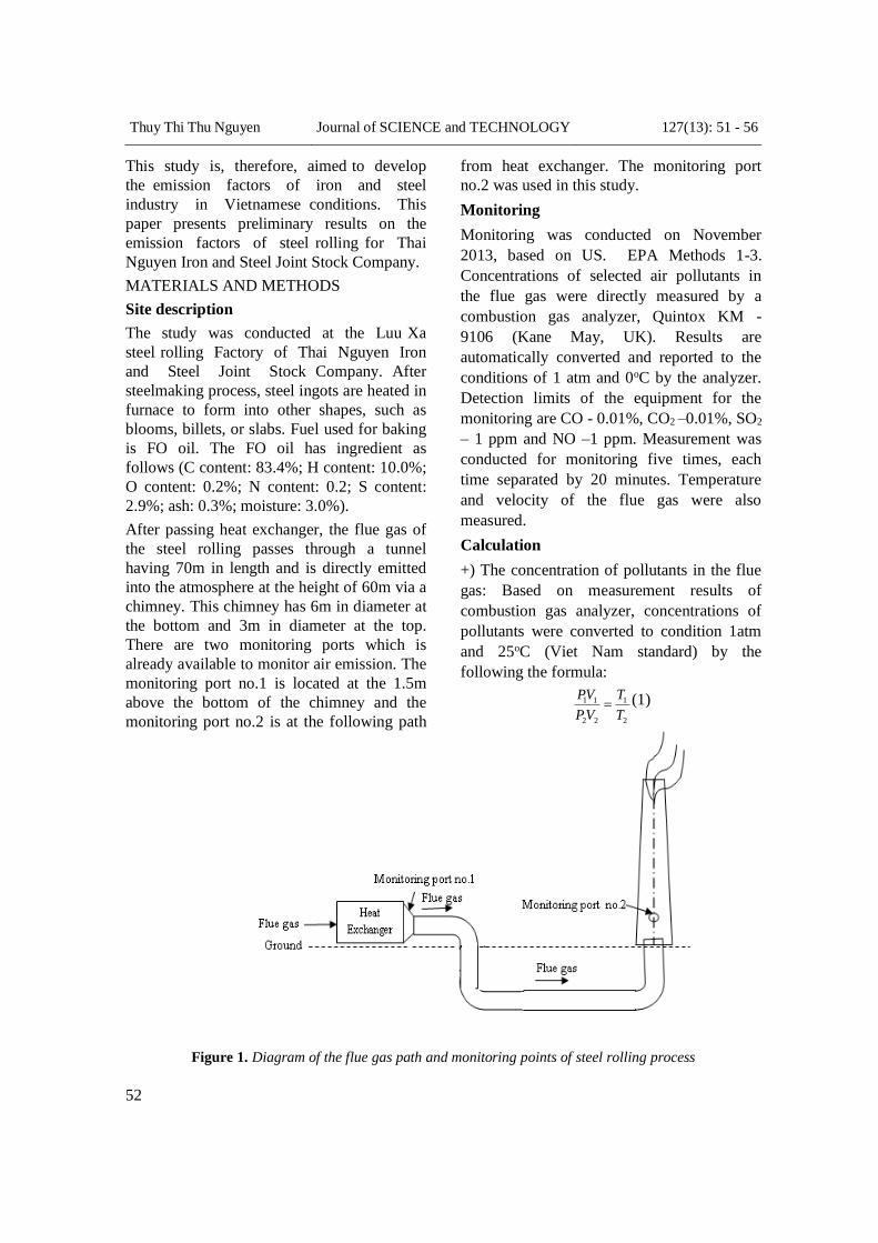
Thuy Thi Thu Nguyen Journal of SCIENCE and TECHNOLOGY 127(13): 51 - 56
52
This study is, therefore, aimed to develop
the emission factors of iron and steel
industry in Vietnamese conditions. This
paper presents preliminary results on the
emission factors of steel rolling for Thai
Nguyen Iron and Steel Joint Stock Company.
MATERIALS AND METHODS
Site description
The study was conducted at the Luu Xa
steel rolling Factory of Thai Nguyen Iron
and Steel Joint Stock Company. After
steelmaking process, steel ingots are heated in
furnace to form into other shapes, such as
blooms, billets, or slabs. Fuel used for baking
is FO oil. The FO oil has ingredient as
follows (C content: 83.4%; H content: 10.0%;
O content: 0.2%; N content: 0.2; S content:
2.9%; ash: 0.3%; moisture: 3.0%).
After passing heat exchanger, the flue gas of
the steel rolling passes through a tunnel
having 70m in length and is directly emitted
into the atmosphere at the height of 60m via a
chimney. This chimney has 6m in diameter at
the bottom and 3m in diameter at the top.
There are two monitoring ports which is
already available to monitor air emission. The
monitoring port no.1 is located at the 1.5m
above the bottom of the chimney and the
monitoring port no.2 is at the following path
from heat exchanger. The monitoring port
no.2 was used in this study.
Monitoring
Monitoring was conducted on November
2013, based on US. EPA Methods 1-3.
Concentrations of selected air pollutants in
the flue gas were directly measured by a
combustion gas analyzer, Quintox KM -
9106 (Kane May, UK). Results are
automatically converted and reported to the
conditions of 1 atm and 0oC by the analyzer.
Detection limits of the equipment for the
monitoring are CO - 0.01%, CO2 –0.01%, SO2
– 1 ppm and NO –1 ppm. Measurement was
conducted for monitoring five times, each
time separated by 20 minutes. Temperature
and velocity of the flue gas were also
measured.
Calculation
+) The concentration of pollutants in the flue
gas: Based on measurement results of
combustion gas analyzer, concentrations of
pollutants were converted to condition 1atm
and 25oC (Viet Nam standard) by the
following the formula:
1 1 1
2 2 2
PV T
PV T (1)
Figure 1. Diagram of the flue gas path and monitoring points of steel rolling process

Thuy Thi Thu Nguyen Journal of SCIENCE and TECHNOLOGY 127(13): 51 - 56
53
Where: P1, V1, T1 are the pressure, the volume
and the temperature of flue gas at actual
condition, respectively and P2, V2, T2 are the
pressure, the volume and the temperature of
flue gas at standard condition.
+) Emission: The total emission of each
pollutant is calculated by the following
formula:
Total emission = Ci.L.t (mg) (2)
Where, Ci is the concentration of each pollutant
(mg/m3), L is the flow of flue gas (m3/h) and t (h)
is monitoring time.
+) Emission factors: The emission factors of each
pollutant are calculated by the following formula
EFi = Ei
(3) Efuel/Eproduct
Where, EFi is the emission factor of each
pollutant, Ei is the emission of each pollutant
and Efuel/Eproduct are amount of fuel and
product, respectively.
RESULTS AND DISCUSSIONS
+) Emission
Average concentrations of the pollutants in
the flue gas of steel rolling process were
calculated following the formula (1) and
shown in Table 1. As seen from table 1, the
concentration of SO2 exceeded the respective
limit values of QCVN 19: 2009/BTNMT
(column B) [19]. However, CO concentration
in the flue gas was not so high and did
not exceed the respective standard of
QCVN19:2009/BTNMT [19] while the
concentration of CO2 was very high. These
results were very logical to explain. When FO
oil in furnace was sprayed under compressed
air pressure of 2Kg/cm2, the contact area
between oil and hot air would rise and
combustion process took place completely. In
addition, the excess air coefficient which had
greater value also lead to complete
convertibility of the Sulfur and Carbon in the
fuel to SO2, CO2.
The concentration of NO in this study was
consistent with the theoretical concentration
of NOx which approximates 700 mg/Nm3 (600
ppm) when excess air coefficient was 20-25%
[20]. Based on the monitoring data, the total
emission in a shift was calculated by the
formula (2) as shown in Table 2. The time of
this shift was 7.67 hours (460 minutes).
Table 1. Summary information of the flue gas of steel rolling process
Sample Temperature
T (oC)
Flow rate
(Nm3/h)
Concentration
CO
(mg/Nm3)
SO2
(mg/Nm3)
NO
(mg/Nm3)
CO2
(g/Nm3)
CT1 423.8 10970 4.92 1239.84 711.85 129.31
CT2 424.5 10568 5.90 1273.27 718.73 129.31
CT3 422.6 10597 5.90 1272.29 713.82 127.51
CT4 423.3 10194 4.92 1262.46 711.85 125.71
CT5 425.2 10557 6.88 1239.84 712.84 127.51
Average 5.7±0.82 1257.54±6.7 713.8±2.87 127.87±1.50
Table 2. Total emissions of selected of pollutants in steel rolling process
Sample Time
(h)
Flow rate
(Nm3/h)
Emission (g/shift)
CO CO2 SO2 NO
CT1 7.67 10970 413.46 10874969.14 104273.84 59868.57
CT2 7.67 10568 477.98 10476799.73 103164.6 58234.22
CT3 7.67 10597 479.29 10359471.61 103366.14 57993.68
CT4 7.67 10194 384.2 9824832.644 98663.589 55632.74
CT5 7.67 10557 556 10300721.05 100158.8 57585.35
Average 462. 19 10367358.83 101925.39 57862.91

Thuy Thi Thu Nguyen Journal of SCIENCE and TECHNOLOGY 127(13): 51 - 56
54
Table 3. Emission factors of pollutants in steel rolling process
Sample
Emission factors
CO CO2 SO2 NO
(g/kg Fuel) (kg/ton Steel) (g/kg Fuel) (kg/ton Steel) (g/kg Fuel) (kg/ton Steel) (g/kg Fuel) (kg/ton Steel)
CT1 0.12 1.69 3.13 44.42 30.04 0.43 17.25 0.24
CT2 0.14 1.95 3.02 42.79 29.72 0.42 16.78 0.24
CT3 0.14 1.96 2.98 42.32 29.78 0.42 16.71 0.24
CT4 0.11 1.57 2.83 40.13 28.43 0.40 16.03 0.23
CT5 0.16 2.27 2.97 42.08 28.86 0.41 16.59 0.24
Average 0.13±0.02 1.89±0.27 2.99±0.11 42.35±1.54 29.36±0.69 0.42±0.01 16.67±0.44 0.24±0.01
+) Emission factor
Emission factors of each pollutant were
calculated following the formula (3) and these
results are presented in Table 3.
Data on the emission factors of gaseous
pollutants were compared with other studies
such as the document of UNEP, IPCC. The
emission factor of NO in this study can be
considered to be in the same range with those
of these studies. The emission factor of CO2
in this study was less than a half of the
emission factor published by UNEP (80kg/ton
steel product) [21] while the emission of CO
was twice as high as the one promulgated by
IPCC [22]. The emission of SO2 was ten
times higher than the emission factor
published by IPCC and UNEP but it was
relatively similar to the emission of SO2 of
boiler using FO oil if the fuel has the same
sulfur content. The difference of these results
can be completely understood because
emission factor depends on several factors
including fuel quality, conditions of
combustion/process, air pollution control
system, etc.
CONCLUSIONS
Emission factors of selected air pollutants
being CO, CO2, SO2 and NO for steel
rolling process of Thai Nguyen Iron and Steel
Joint Stock Company were determined.
This is a significant contribution to
Vietnam database of emission factors steel
rolling process in particular and for iron
and steel industry in general. These emission
factors can be used for emissions inventory
and air quality management at the company.
Methodology used in this study can be
applied to other iron and steel industrial
enterprises in the country.
REFERENCES
1. US Environmental Protection Agency
"Compilation of Air Pollutant Emission Factors,
AP-42, 5th Ed", 2002.
2. WHO "Assessment of sources of air, water, and
land pollution, A guide to rapid source inventory
techniques and their use formulating
environmental control strategies"; Part 1: Rapid
inventory techniques in environmental pollution,
1993.
3. Etui-Chan Jean, Someone Myeong, Jae-Whan Sa,
Jinsu Kim, Jae-Hak Jeong, “Greenhouse gas emission
factor development for coal-fired power plants in
Korea”, Applied Energy, Volume 87, Issue 1, January
2010, Pages 205–210.
4. Yu Zhao, Shuxiao Wang, Chris P. Nielsen,
Xinghua Li, Jiming Hao, “Establishment of a
database of emission factors for atmospheric
pollutants from Chinese coal-fired power plants”,
Atmospheric Environment, Volume 44. Issue 12,
April 2010, Pages 1515–1523.
5. S.Nazari, O.Shahhoseini, A.Sohrabi-Kashani,
S.Davari.R.Paydar, Z. Delavar - Moghadam,
“Experimental determination and analysis of CO2,
SO2 and NOx emission factors in Iran’s thermal
power plants”, Energy, Volume 35, Issue 7, July
2010, Pages 2992–2998.
6. Hoang Duong Tung, Nguyen Thi Nguyet Anh
et al, Research on establising emission factors for
pollutant inventory from road transport, Ha Noi,
Environmental Monitoring Centre, 2010
7. Ho Minh Dung, Dinh Xuan Thang,
“Establishment of emission factors from road
transport in Ho Chi Minh city ”, Journal of Labor
Protection, 2009.

Thuy Thi Thu Nguyen Journal of SCIENCE and TECHNOLOGY 127(13): 51 - 56
55
8. Ta Thu Huong, Le Anh Tuan and Nghiem Trung
Dung, “Preliminary estimation of emission factors for
motorcycles in real-world traffic conditions of Hanoi”,
Journal of Science and Technology, vol. 48, issue 3,
2010, page 101-110
9. Nguyen Thu Trang, Nghiem Trung Dung, Tran
Thu Trang, “Potentiality of co-benefits of climate
and air quality in fuel switching for Hanoi Bus
system”, Journal of Science and Technology, vol. 49,
issue 4, 2011, page 75-86.
10. Nguyen Thi Kim Oanh, Larsbæ Tzreutergårdh
and Nghiem Trung Dung, “Emission of Polycyclic
Aromatic Hydrocarbons and Particulate Matter
from Domestic Combustion of Selected Fuels”,
Environmental Science and Technology, 1999,
pages 2703-2709.
11. Nghiem Trung Dung. Hoang Xuan Co. Pham
Ngoc Ho. Dong Quang Huy. “Emission of
polycyclic aromatic hydrocarbons and particulate
matter from domestic cooking using coal”. Tạp chí
Journal of Applied Chemistry. Vol. 11, 2004. page
31-34
12. Nghiem Trung Dung, Hoang Xuan Co, Pham
Ngoc Ho, Dong Quang Huy, “Emission of
polycyclic aromatic hydrocarbons and particulate
matter from domestic cooking using sawdust”,
Journal of Science and Technology, vol. 43, issue 1,
2005, page 108-113
13. Nghiem Trung Dung, Nguyen Viet Thang,
“Determination of emission factors for domestic
sources using biomass fuel”, Journal of Science
and Technology, No 82A, 2011, pages 32-36
14. Nghiem Trung Dung, Le Phuong Thuy,
“Determination of emission factors for domestic
sources using fossil fuel”, Journal of Science and
Technology, No 82A, 2011, pages 32-36
15. Nghiem Trung Dung. Larsbæ Tzreutergårdh.
Nguyen Thi Kim Oanh. Dang Lim Chi. Hoang
Xuan Co. “Emission of polycyclic Aromatic
Hydrocarbons associated with particulate matter
from a coal-fire power plant in Vietnam”. Journal
of Applied Chemistry. Vol. 9, 2004. page 36-40
16. Nguyen Thi Thu Thuy “Determination of
emission factors for steel rolling using FO oil”,
Thai Nguyen Journal of Science and Technology,
No 12, 2011
17. Nguyen Thi Thu Thuy, Nghiem Trung Dung,
“Determination of emission factors for coke
quenching”. Journal of Science and Technology,
No 87, 2012, pages 62-66
18. Nguyen Thi Thu Thuy, “Determination of
emission factors for coke quenching and sintering
in iron and steel industry”, International
Symposium on Technology for Sustainability
Workshop, Bangkok, Thailand, 2012.
19. MONRE. “QCVN 19:2009/BTNMT - National
Technical Regulation on Industrial Emission of
Inorganic Substances and Dusts”, Hanoi, 2009.
20. Noel de Nevers, "Air pollution control
engineering", McGraw-Hill, 1995
21. Department of Environmental impact
assessment and appraisal - Vietnam Environment
Administration, “The guide to preparing
Environmental impact assessment reports in cast-
iron and steel plants”, Hanoi, 2009 [22] IPCC
www.ipcc-nggip.iges.or.jp, access date 20/06/2014.

Thuy Thi Thu Nguyen Journal of SCIENCE and TECHNOLOGY 127(13): 51 - 56
56
TÓM TẮT
XÂY DỰNG DỮ LIỆU BỘ HỆ SỐ PHÁT THẢI
CÁC CHẤT Ô NHIỄM KHÔNG KHÍ TRONG QUÁ TRÌNH CÁN THÉP
Nguyễn Thị Thu Thủy*
Trường Đại học Kỹ thuật Công nghiệp – ĐH Thái Nguyên
Từ lâu hệ số phát thải đã được coi như một công cụ hiệu quả về kinh tế trong kiểm kê khí thải. Tuy
nhiên, dữ liệu về hệ số phát thải còn khá khan hiếm tại các nước đang phát triển trong đó có Việt
Nam. Nghiên cứu này được thực hiện để xác định hệ số phát thải của CO, CO2, SO2 và NO trong
quá trình cán thép. Nồng độ các chất ô nhiễm được đo đạc bằng thiết bị đo nhanh - Quintox KM-
9106 - tại công ty Gang thép Thái Nguyên. Tổng lượng phát thải chất ô nhiễm và hệ số phát thải
của từng chất đã được tính toán dựa trên kết quả quan trắc và thông tin về quá trình. Tính theo
nhiên liệu, hệ số phát thải của CO, CO2, SO2 và NO tương ứng là 0,13 g/kg; 2990 g/kg; 29,36 g/kg
và 16,67 g/kg. Theo sản phẩm, hệ số phát thải của CO, CO2, SO2 và NO tương ứng là 1,89 kg/ton;
42,35 kg/tấn; 0,42 kg/tấn và 0,24 kg/tấn. Kết quả đạt được trong nghiên cứu này có thể được sử
dụng trong kiểm kê phát thải công nghiệp và quản lý môi trường không khí tại Việt Nam
Từ khóa: Hệ số phát thải, cán thép, dầu FO, ô nhiễm không khí, kiểm kê phát thải.
* Tel: 0979958785; Email: [email protected]

Duy Nguyen Tien et al Journal of SCIENCE and TECHNOLOGY 127(13): 57 - 62
57
DISSOLVED OXYGEN CONTROL OF THE ACTIVATED SLUDGE WASTEWATER TREATMENT PROCESS USING HEDGE ALGEBRAICCONTROL
Duy Nguyen Tien, Binh Lam Hoang, Son Lam Hung, Huy Nguyen Phuong*
University of Technology - TNU
ABSTRACT
Activated sludge wastewater treatment process is difficult to be controlled because of its complex,
time-varying and non-linear behavior. In this process, the control of the dissolved oxygen (DO)
concentration in the reactors plays an important role in the operation of the facility.In addition to
evaluating some controllers for DO such as PI, FLC, this paper also introduces a new approach,
using Hedge Algebraic (HA). The results show that Hedge Algebraic Controller (HAC) can be
effectively used for DO control in activated sludge wastewater treatment process.
Keywords: Hedge Algebraic control, Dissolved Oxygen control, Wastewater treatment.
INTRODUCTION*
Aeration is an important part of the whole
activated sludge wastewater treatment process
because aerobic conditions are conducive to
the growth of a wide variety of microbes,
including heterotrophic bacteria, which
remove biochemical oxygen demand (BOD)
from the wastewater, as well as nitrifying
bacteria, which oxidize ammonia to nitrate.
Because of the strong and fast effects of
aeration on biomass growth, DO control is the
most studied control problem in wastewater
treatment 1. DO control is the difficulty and
focus of biological wastewater treatment
processes. Insufficient or excess oxygen in
the aeration tank will lead to the deterioration
of activated sludge.
In the past, most of the DO control systems
reported in literature employ classical PI
controllers, which are mainly because of the
inherent simple design and application, and
mostly satisfactory performance in the
operating range of interest.
Fuzzy controllers (FLC) have much superior
in quality compared with PI controller.It is
often pointed out that FLCs do not require
knowledge of a detailed mathematical model
of the control system and allow a more
intuitive approach to design compared to the
* Tel: 0912488515; Email: [email protected]
PI controller because the fuzzy sets used in
fuzzy control aim to capture the semantics of
natural linguistic terms present in the fuzzy
controller knowledge. In addition, they have
the capability of handling uncertain and noisy
signals, and usually lead to better results
compared to the classical PI controller in
terms of response time, settling time and
robustness 5.
Hedge algebras were developed in 2 to model
the order-based semantics of the terms in
term-domains of linguistic variables. Then,
the fuzzy rules can be viewed as to define
points in a Cartesian product of suitable
hedge algebras, and approximate reasoning
method on the controller knowledge can be
transformed into an interpolation method on a
real surface defined by these points by using
fuzziness parameters values 3. Since this
transformation is defined by Semantically
Quantifying Mappings (SQMs) of hedge
algebras, which may preserve the relations
between the variables based on the order-
based semantic of terms in the controller
knowledge, the resulting surface can be
considered as an appropriate mathematical
model of the controller knowledge. So, hedge
algebras may provide a sound formalized
basis to develop effective new reasoning
methods for a kind of controllers, called
hedge algebra (HA) controllers.

Duy Nguyen Tien et al Journal of SCIENCE and TECHNOLOGY 127(13): 57 - 62
58
In this paper, in addition to evaluating some
controllers for DO such as PI, FLC, this paper
also introduces a new approach, using HAC.
The results show that HAC cang be
effectively used for DO control in activated
sludge wastewater treatment process.
HEDGE ALGEBRA CONTROLLER OVERVIEW
Hedge algebras (HAs) are aimed to show that
the inherent ordered-based structures of term-
domains of linguistic variables are useful to
discover order-based semantic properties of
terms and term-domains 23. On this
viewpoint, every term-domain of a linguistic
variable X can be considered as an HA, AX =
(X, G, C, H, ), where X is a term-set of X;
is an order relation on X, which is regarded as
to be induced by the inherent order-based
semantics of the terms of X; G = {c–, c+},
where c– (or, c+) is called the negative (or,
positive) primary term, is the set of generators
that satisfy c– c+; C = {0, W, 1} is the set of
constants satisfying 0 ≤ c– ≤ W ≤ c+ ≤ 1,
whose meanings state that 0 and 1 are,
respectively, the least and the greatest term in
X, W is the neutral term; H = H– H+, where
H– = {hj: 1 j q} is the set of negative
hedges hH satisfying hc+ c+ (written as
sign (h) = 1) and H+ = {hj: 1 j p} is the
set of positive hedges h satisfying hc+ ≥ c+
(written as sign (h) = +1). Since hj’s are
regarded as unary operations, every term of
AX, except from the constants, is of the form
hnhn-1 ... h1c, c G. Many inherent semantics
properties of terms and, especially, hedges
can be discovered in the structure of AX. For
instance, hx and x are always comparable, for
every x X and h H; assuming that hx ≥ x,
the comparability of hx and khx implies that
either khx ≥ hx ≥ x, which is indicated by
sign(k, h) = +1, or hx ≥ khx ≥ x, which is
indicated by sign(k, h) = 1. E.g. we can
check that sign(V,L) = +1, as Vlbig ≤ Lbig
≤big, while sign(V,R) = 1, as
Rbig≤VRbig≤big. Then, every xX\C has a
sign defined by Sgn(x) = sign(hn, hn-1) …
sign(h2h1)sign(h1)sign(c), where x = hnhn-1 …
h1c, for c G. It is proved that Sgn(hx) = 1
hx ≤ x and Sgn(hx) = +1 hx ≥ x.
The semantic structure of AX discovered in
the algebraic approach to the term semantics
implies that the set HI(x) = {x = hnhn-1 ... h1c :
cG, hjH }{x}, for every xX, can be
considered as the model of the fuzziness of x.
The structure of the set of all such sets, H(x),
xX, induces a fuzziness measure fm of the
terms of X, which is equal to the “diameter”
of H(x) and can be calculated by given
fuzziness measure of the primary terms,
fm(c) and fm(c+), and the fuzziness measure
of hedges, (h), h H, called commonly the
fuzziness parameters of X. We have that for
every x X,x = hnhn-1 ... h1c,
Gccfmhhchhhfm nnn ),()()...()...( 111 (1.1)
In turn, a given fuzziness measure fm of X
induces numeric term semantics, defined by
the so-called Semantically Quantifying
Mapping (SQM) fm, which is also calculated
by the given fuzziness parameter values as
follows:
( )
( ) ( ), ( ) ( )
( ), ( ) ( )
( ) ( )
( ) ( ) ( ) ( )
fm fm
fm
fm j fm
j
j i j ji sign j
W fm c c fm c
fm c c fm c
h x x
Sgn h x fm h x h x fm h x
(1.2)
where
,))(()(12
1)( xhhSgnxhSgnxh jpjj
for all integers j[q^p]=[q, p]\{0}.
DESIGN HAC FOR DISSOLVED OXYGEN
CONTROL
Dissolved Oxygen Control of the Activated
Sludge Wastewater Treatment Process
The general overview of activated sludge
wastewater treatment process is shown in
Fig.1. The inflow is first processed in the
bioreactor where, by the action of
microorganisms, the substrate content is
reduced. Next, the water flows to a settler,
where the biomass sludge is recovered. The
clean water remains at the top of the settler
and is carried out of the plant, and a fraction
of the sludge is returned to the input of the
bioreactor in order to maintain an appropriate
level of biomass, allowing the reduction of

Duy Nguyen Tien et al Journal of SCIENCE and TECHNOLOGY 127(13): 57 - 62
59
the organic matter. The rest of the sludge is
purged 9.
A block diagram of the DO controller is
shown in Fig2. According to [8], DO transfer
function is given by:
(2.1)
Where K=0.8, T1=12, T2=100, =60.
In order to verify responses of these
controllers when changing of DO, the
expected value of the DO areset in Table 1.
Determination of hedge algebras for the
linguistic L-variables and linguistic rule base
First, it is necessary to specify the same sets
G, C and H for all the required HAs as
follows:
1) The set G of the primary terms is assumed
to be {S, B}, i.e. the negative primary term
c = S (Small) and the positive primary term
c+ = B (Big).
To express the semantics of terms present in
fuzzy model, it is sufficient to define
H– = {L (Little)} and H+ = {V (Very)}.
The whole term-set X of every HA is then
completely determined, regardless its term-set
is finite or infinite. Examples of terms are B
(Big), VB (Very Big), S (Small) and so on.
Then, the HA-terms with length of one or two
is established as in Table 2. However, since
there are only five labels of the variables Le
and Lce, their term-transformations are
established. All the established transformations
should preserve the order-based relationships
and the opposite meaning of terms, e.g. the
opposite terms VS and VB are of opposite
meaning.
Table1. The expected value of the DO with time
t [s] 0 – 200 200– 400 400 – 600 600 – 800 800 – 1000
*
dcu [mg/l] 2 3 4 1 2
Figure 1. General overview of activated sludge wastewater treatment process8
Figure 2. A block diagram of the DO controller
Controller Air-blower
Oxygen mass
transfer
de/dt
+ -
ec
u y

Duy Nguyen Tien et al Journal of SCIENCE and TECHNOLOGY 127(13): 57 - 62
60
Table 2. Term transformation of the linguistic
variable Lu
For FL NB N ZE P PB
Linguistic
Variable Lu VS S W B VB
linguistic
variables Le
and Lce
S LS W LB B
Determination of the mathematical model
of the given rule base for desired HA
controller
The HA rule base is represented in Table 3.
The linguistic values of their cells can be
determined based on the monotonicity of the
linguistic terms in either the respective
column or row, i.e. they can be drawn
intuitively from the given rule base.
Table 3. Rule base for the HA controller
Lce
Le S LS W LB B
S VS VS VS S W
LS VS VS S W B
W VS S W B VB
LB S W B VB VB
B W B VB VB VB
To determine the mathematical model of Sreal
of the rule base with HA-terms given in Table
3, the fm-values of the terms of every
variable present in Table 4 must be computed
by applying Eqs. (1.1) and (1.2), examined in
more detail in 5, for determining SQM fm,
induced by a given fuzziness measure fm of
every variable. However, here for the terms in
Table 3, which are of only length not greater
than 2 and generated by the use of only two
hedges in H = {h-1, h1}, i.e. every term
contains at most one hedge which is either h-1
or h1, Eqs. (1.1) and (1.2) can be rewritten
simply as follows, noting that, as i = sign(j) =
j {-1, 1}.
Calculated with Eq (1.1) and Eq (1.2), a grid
of the points of the surface Sreal corresponding
to all the linguistic points defined by the cells
of Table 4 can be calculated and obtained as
presented in Table 5. Now, an ordinary
interpolation method on Sreal can simply be
selected as an HA-IRMd. It can be observed
observe again that once an HA-IRMd is
selected, all components of the designed HA
controller can completely be determined by
merely the independent fuzziness parameters
of the variables Le, Lce and Lu. Thus, as there
are not many numeric interpolation methods
to be selected, it is useful that to enhance the
performance of the designed controller it is
only necessary to determine appropriate
fuzziness parameters values of the linguistic
variables, as presented in Table 4.
Determination of the quantitative semantics
of terms for each linguistic variable
Once the HAs of the variables are determined,
the determination of their quantitative term
semantics is simply to specify values of the
fuzziness parameters of the variables. For
simplification, these parameter values were
determined in Table 4, noting that always
fm(B) + fm(S) = 1 and μ(L) + μ(V) = 1. Using
these parameters values all the terms in Table
4 can be computed, which means that the
surface Sreal is determined approximately.
Table 4. Determined parameters Values of Le,
Lce and Lu
Le Lce Lu
fm(S) 0.5 0.5 0.5
= μ(L) 0.3 0.3 0.7
All the linguistic points represented in Table
3 are transformed into the points shown in
table 5.
The points shown in Table 5 determine
approximately the surface Sreal as represented
in Fig. 3.
Figure 3. Surface Sreal for the HAC

Duy Nguyen Tien et al Journal of SCIENCE and TECHNOLOGY 127(13): 57 - 62
61
Table 5. SQM-values of the HA-terms
e
ce
0.350
(S)
0.455
(LS)
0.500
(W)
0.545
(LB)
0.650
(B)
0.350
(S)
0.045
(VS)
0.045
(VS)
0.045
(VS)
0.150
(S)
0.500
(W)
0.455
(LS)
0.045
(VS)
0.045
(VS)
0.150
(S)
0.50
(W)
0.850
(B)
0.500
(W)
0.450
(VS)
0.150
(S)
0.500(
W)
0.850
(B)
0.955
(VB)
0.545
(LB)
0.150
(S)
0.500
(W)
0.850
(B)
0.955
(VB)
0.955
(VB)
0.650
(B)
0.500
(W)
0.850
(B)
0.955
(VB)
0.955
(VB)
0.955
(VB)
Simulations
In order to evaluating effectiveness of HAC for
DO, we also design PI control and FLC.
Parameters of the PI controller for DO is
KP = 5.2, TI = 0.1. Parameters of the FLC is
corresponded to HAC. The results are showed
in Fig 4.
Fig 4 shows responses of these controller to
the change of the reference DO over time. For
the classic PI controller, the response has the
largest overshoot/undershoot and the longest
establishment time. These values were
significantly reduced for FLC. And
especially, the HAC response is the best of
overshoot/undershoot and establishment time.
CONCLUSIONS
In this paper, a new type of controller based
on hedge algebra was proposed and applied
for Dissolved Oxygen Control of the
Activated Sludge Wastewater Treatment
Process. To our best knowledge, this is the
first time that the hedge algebra principles
were successfully applied in this field. The
effectiveness of the proposed approach was
evaluated through comparison with both the
classical PI controller and the FL controller.
The simulation was performed and the results
were gathered in reasonably wide ranges of
the DO. Based on the obtained results, the
developed HA controller proved to be the best
choice for the purpose out of the considered
controllers because of its superior
performance in terms of tracking the
reference DO and robustness. More
specifically, it was shown that only the HA
controller manages to reconcile the
requirements for fast response and small
overshoot/undershoot. At the same time, its
computational efficiency was shown to be
satisfactory and similar to that of the other
two considered controllers. The newly
developed HA controller was definitely
proven to be research worthy and a promising
alternative to the existing solutions in the
field of control engineering.
Figure 4. Simulation results of PI controller, FLC, HAC for DO

Duy Nguyen Tien et al Journal of SCIENCE and TECHNOLOGY 127(13): 57 - 62
62
REFERENCE
1. C. A. C. Belchior, R. A. M. Araújoa, J. A. C.
Landeckb, Dissolved oxygen control of the
activated sludge wastewater treatment process
using stable adaptive fuzzy control, Computers
and Chemical Engineering, 37: 152-162, 2012.
2. C.H. Nguyen, W. Wechler, Hedge algebras:
An algebraic approach to structures of sets of
linguistic domains of linguistic truth variable,
Fuzzy Set. Syst., 35 (1990) 281-293.
3. C.H. Nguyen, N. L. Vu, X. V. Le, Optimal
hedge-algebra-based controller: Desgn and
application, Fuzzy Set. Syst., 159 (2008) 968-989.
4. C.H. Nguyen, N. L. Vu, X. V. Le, Quantifying
hedge algebras, interpolative reasoning method
and its application to some problems of fuzzy
control, WSEAS T. Comput., 5 (2006) 2519-2529.
5. C.H. Nguyen, D.A. Nguyen, N.L. Vu, Fuzzy
Controllers Using Hedge Algebra Based
Semantics of Vague Linguistic Terms, in: D.
Vukadinović (Ed.), Fuzzy Control Systems, Nova
Science Publishers, Hauppauge, 2013, pp. 135-
192.
6. J.M. Zurada, R.J. Marks, C.J. Robinson,
Computational Intelligence Imitating Life, IEEE
Press, Piscataway, 1994.
7. S.R. Buss, 3D Computer Graphics: A
Mathematical Introduction with OpenGL,
Cambridge University Press, New York, 2003.
8. YE Hong-tao, LI Zhen-qiang, LUO Wen-
guang, Dissolved Oxygen Control of the Activated
Sludge Wastewater Treatment Process Using
Adaptive Fuzzy PID Control, Proceedings of the
32nd Chinese Control Conference, pp 7510-7513,
2013
9. W. C. Chen, N. B. Chang, J. C. Chen, Rough
set-based fuzzy neural controller design for
industrial wastewater treatment, Water Research,
37 (1): 78-90, 2003.
10. Jain, L.C., and Jain R.K.: “Hybrid
Intelligent Engineering Systems”, World
Scientific Publishing, 1997.
TÓM TẮT
ỨNG DỤNG ĐẠI SỐ GIA TỬ ĐỂ THIẾT KẾ BỘ ĐIỀU KHIỂN
LƯỢNG OXY HÒA TAN TRONG QUÁ TRÌNH XỬ LÝ NƯỚC THẢI
THEO PHƯƠNG PHÁP BÙN HOẠT TÍNH
Nguyễn Tiến Duy, Lâm Hoàng Bình, Lâm Hùng Sơn, Nguyễn Phương Huy*
Trường Đại học Kỹ thuật Công nghiệp – ĐH Thái Nguyên
Xử lý nước thải bằng phương pháp bùn hoạt tính là một quá trình điều khiển khó khăn do hệ thống
phức tạp, biến đổi theo thời gian và có tính chất phi tuyến. Trong quá trình này, việc điều khiển
lượng oxy hòa tan (DO) tập trung ở các lò phản ứng đóng vai trò rất quan trọng trong hoạt động
thực tế của hệ thống. Trong bài báo này, ngoài việc đánh giá việc điều khiển DO theo các phương
pháp như PI, FLC, các tác giảcòn giới thiệu một cách tiếp cận mới, sử dụng đại số gia tử (HA).
Các kết quả thu được cho thấy các bộ điều khiển sử dụng đại số gia tử kiểm soát hiệu quả hơn
nồng độ DO trong quá trình xử lý nước thải theo phương pháp bùn hoạt tính.
Từ khóa: Bộ điều khiển dùng đại số gia tử, điều khiển oxy hòa tan, xử lý nước thải.
* Tel: 0912488515; Email: [email protected]

Khuyen Thi Minh Pham et al Journal of SCIENCE and TECHNOLOGY 127(13): 63 - 68
63
SUPPLY CHAIN MANAGEMENT FOR COLLEGES/UNIVERSITIES: SOLUTIONS TO IMPROVE THE EFFICIENCY OF THE TRANSFER OF SCIENCE AND TECHNOLOGY
Khuyen Thi Minh Pham*, Yen Thi Mai Pham
University of Technology – TNU
ABSTRACT
The Integrated Educational Supply Chain Management (IESCM) for the colleges and universities
provides two main contributions to the society, including human resource contribution and
research contribution through two main activities of colleges/universities: education and research.
In the world, theories about Educational Supply Chain were studied in the last years of the 90s,
but in Vietnam these contents are still new. This article depicts a holistic view, comprising inputs,
the process, and outputs of the educational supply chain. With the analysis about three group
activities of supply chain management and some experiences from education developing
countries, the paper also provides educational management a new dimension to understand how
supply chain management contributes to successful university operations, especially enhances the
efficiency of scientific and technological transfer.
Keywords: The Integrated Educational Supply Chain Management (IESCM), Efficiency of scientific and
technological transfer, Relationship Management, Social Orientation, Strategy.
INTRODUCTION
In recent times, the theory of supply chain
management (SCM) has been widely studied
under a variety of labels and for a number of
reasons: improving operations, better
outsourcing, increasing profits, enhancing
customer satisfaction, generating quality
outcomes, tackling competitive pressures,
increasing globalization, increasing
importance of E-commerce, and growing
complexity of supply chains.
In the world
The first theory about supply chain
management appeared in 1950s with the
development of goods and relationships in
businesses... and it rapidly widened their
applications to other fields of life. (Fig 1)
It is a surprising fact that researchers
developed SCM models focusing mostly on
improving business operations. Few,
particularly academic researchers, do not
realize that the research on academic supply
chain management may also be conducted for
their own educational institutions.
Figure 1. Timeline of theory in Supply chain management*
* Tel: 01688140486Email: [email protected]
195
0
197
0
199
0
201
0
Initiated Logistic Concept Initiated the SCM Concept
1980
Matured Logistic Concept 1985
SCM in the Manufacturing Industry
1995
Initiated SCM in the Service Industry
2007
Education SCM
ITE SCM
2009
Redesigned ITESCM
2012

Khuyen Thi Minh Pham et al Journal of SCIENCE and TECHNOLOGY 127(13): 63 - 68
64
Until 1996, O’Brien [1] proposed an
educational supply chain as a tool for
strategic planning in tertiary education. The
study was based on a survey among
employers and students. Survey findings
revealed that integration and coordination
among students and employers should have
been promoted. In 2007, Lau [2] performed
an in-depth case study approach to developing
an educational supply chain management for
the City University of Hong Kong. In fact,
Educational supply chain represents
international supply chain management
concept as it is the uniform dimension for the
international arena (Habib, 2008-2012) [3].
In Vietnam
The concepts of SCM are rather new with
Vietnamese business. The Manager started
considering the theory of SCM in some recent
years when Vietnam became a member of
WTO and they had to face with the strong
competition of global companies. But, almost
researches focused on the SCM in
manufacturing industry.
LITERATURE REVIEW
Model of supply chain for colleges/
universities
The objective of the educational supply chain
is to develop the quality graduates and
researches with limited resources for the
society, which is the final customer or
consumer. To achieve this goal, educational
institutions need to have a certain degree of
knowledge about the partners in their supply
chains including suppliers, customers, and the
consumer. (Fig 2)
Suppliers
Education Suppliers include: Suppliers of the
student (high schools/colleges); Suppliers of
the faculty (Other universities/colleges);
Source of fund – Family (Parents, siblings),
relatives, etc; Government and private
organizations (Scholarship); Suppliers of
assets or equipment (Furniture, computer,
networking equipment, etc.); Suppliers of
educational materials (Stationery, instruction
materials, etc.);
Research Suppliers include: Suppliers of
Internal Research Projects (University self
funding); External research projects (External
research funds, Ministry of Education, private
organizations, etc.)
Figure 2. Model of Educational Supply chain for Colleges/universities [4]
Graduates Research
Education customers Research Customers
Society
Education Supplier Research Supplier
Pupils Research
projects
Academic Strategies, plans,
operation and quality
Research Strategies, plans,
operation and performance
evaluation.
Colleges/Universities
PE UC FC FA PE UC FC FA PE: Programs Establishment
UC: Universities culture
FC: Faculty Capabilities
FA: Facilities

Khuyen Thi Minh Pham et al Journal of SCIENCE and TECHNOLOGY 127(13): 63 - 68
65
Activities of colleges/universities
A university is regarded as a service provider
with 2 main services: Education and
Research. Through proper educational
management, the university can produce
quality outcomes for the society.
Factors influence on the supply chain for
colleges/universities often are Programs
Establishment (PE), Universities culture
(UC), Faculty Capabilities (FC), Facilities
(FA). In Vietnam, it also be depend on the
management and regulation of government.
Outcomes
Graduates: Quality of graduates often
include: Knowledge (Tacit or Explicit), skills,
competencies, capabilities, ethics, career
Development Programs
Researches: Quality research outcomes may
include problem solution, pure theory, thesis
findings, internal and external projects
applications, researchers, research
publications, or research findings, etc.
Customers
EEducation Customers: Graduates, family
(parents, siblings, relatives, etc.),
employers of government and private
organizations.
Research Customers: Funding organizations
of research projects, research outcomes
(researchers, research publications, findings
etc.), Others (research professional
organizations, Society of manufacturing
engineers and Trade Associations, etc.).
Consumers
The society is the end customer in
educational supply chain. As
colleges/universities are the part of the
society, the final outcomes of this supply
chain, including graduates with desirable
quality and quality research outcomes are
delivered to the society.
The activities in supply chain management
for colleges/universities and their effects to
the transfer of science & technology
There are three groups of activities in supply
chain management for Colleges/universities.
Operate the activities of Colleges/universities with Society orientation
In educational management, three decision levels are involved in the process of the university: 1. Strategic Level- general direction, long-term goals, philosophies and values; 2: Planning Level: decisions support strategic decisions; 3: Operating Level: every day decisions, Operational decisions can be pre-programmed, pre-made, or set out clearly in policy manuals. These decision should be based on the social need for human resources and researches and abilities of colleges/universities.
Relationship management with suppliers
Raw material in educational supply chain for colleges/universities are pupils in high school and other colleges and they take an importance part in the success of education process. Pupils need to be career oriented early and clearly to have good preparation and attitude to study in colleges/universities . This is only achieved when universities and schools have a good relationship with each others. Good relationship with high schools also help colleges/universities have advantage in attracting pupils.
Research Suppliers are specially important with research supply chain for colleges/universities because they supply fund and information for research. colleges/universities want to become research colleges/universities need have a big self research funding and lots of External research funds.
Relationship management with customers
Relationship management between colleges/universities and Businesses represented by their co-operations:
1. Cooperation in Research: The purpose of this collaboration is to achieve support for research activities of the colleges/universities, implementing projects that link the academic world and the business conduction.
2. Commercialization of research results: It includes technology transfer. In developing countries like Vietnam, to be able to promote this form of cooperation, it is necessary to do immediately is to strengthen the institutional framework to ensure the actual intellectual property rights.

Khuyen Thi Minh Pham et al Journal of SCIENCE and TECHNOLOGY 127(13): 63 - 68
66
3. Promote mobility of students: by creating mechanisms to support them, such as putting students in internships and creating opportunities for them to be able to experience many rich aspects of the world outside the colleges/universities . Strengthen coordination with the human resource department of the company, business to facilitate students to the world of work.
4. Promote the movement of academia: Encourage exchanges or short-term contract work of academics in the business to build relationships, share their views and capture reality.
5. Develop and implement training programs: Improve the quality of education and help students adapt well to the demands of the labor market. It should encourage the involvement of businesses in the construction and renovation of colleges/universities programs, through discussion and information exchange.
6. Support business start-up activities: creating a stimulating cultural faculty and students to think and act with entrepreneurship, put them to the way of the corporate world and attract them to escape the old path of thinking.
These co-operations between businesses and colleges/universities have contributed to social many benefits: Creates new knowledge (through research, reflected by patents, inventions, scientific articles), promotes production (through technology transfer, expressed through economic growth based on knowledge), providing skilled human resources (through training, demonstrated by the number of graduates have jobs).
EXPERIENCES FROM OTHER COUNTRIES
The United State (U.S): High investment from Government and Companies to colleges/universities; Good relationship between high schools, colleges/universities and business
In the U.S., the U.S. government's investment for Science and Technology higher than the same investment in the governments of European countries and Japan combined, while investment in Science and Technology
of the U.S. company 3 times higher than the value of government investment. The policy of the U.S. government is creating conditions for all U.S. citizens to access to education and training they need.
U.S. universities have good relationship
between high schools and Business and its
result is that, currently, one third of the research
in the world of Science and Technology
published annually branded America. 45% of
professors, scientists teaching at U.S.
universities are foreign nationals.
Singapore: colleges/universities are real
businesses, always orient to social [5]
Singapore is well-known as a center of high
technology, have contributed of the
university at international level. They handle
very well the relationship between
universities with businesses around the
exploitation of research results and protection
of intellectual property rights. This experience
is significantly useful for Vietnam. Being the
country's only two full-fledged universities up
to the turn of the century, the National
University of Singapore and Nanyang
Technological University have a strong
tradition of collaborating with industry. Their
graduates continue to find employment
readily in the diverse manufacturing and
service sectors in the country. The culture of
interaction with industry has been developed
through a range of activities including
internships, research collaboration,
technology licensing, adjunct appointments
and industry participation in consultative
committees of academic departments.
LESSONS FOR VIETNAM’S
COLLEGES/UNIVERSITIES
To improve the efficiency of scientific and
technological transfer we need to care about
two main issues: 1) The relevance of science
and technology is transferred to reality; 2)
The capacity of the parties to perform the
transfer. The training institutes in the world
solve these problems by managing the
relationship between the members of the
educational supply chain. In Vietnam, it is
still new lessons.

Khuyen Thi Minh Pham et al Journal of SCIENCE and TECHNOLOGY 127(13): 63 - 68
67
Improve quality of education and research with social orientation
Concentrate on Students is outdated. Enhance education and research quality is not only about improving level of lectures, education programs and services but also all of them to satisfy the social needs.
Many managers of colleges/universities still think that they need to concentrate on needs of students such as their knowledge, their accommodation, their leisure activities,… But, the main and most important purpose of learning in colleges/universities is to get a good job for one’s life. And we can do it only by giving them the knowledge, skills and attitude that the society needs. The number of graduates that have jobs in properly trained field is an important criterion that made the reputation of a institution
The reputation of one College/University also depends on their abilities on research. colleges/universities in Vietnam. The universities of Vietnam are often underestimated in research capacity. We have a lot of professors, doctors but the numbers of researches which are recognized in the region and the world are even lower than the average level of the Southeast Asia region. There are two main reasons are: 1) Lack of orientation mechanisms, support scientific research at both national and Universities levels. 2) Separation to research environment (social demand) of scientists. So, they are the urgent problems that need to change in order to improve the efficiency of scientific and technological research.
Relationship between Colleges/universities and high school
Study the social needs, design right product, show what we need from the supplier and help them supply good raw material is the process to make a suit product and gain a better benefit in a Supply chain. And this process also apply in Educational Supply chain. Help high schools orient the career for the pupils basing on their abilities and dream work to chose right pupils with their love and abilities to study will help colleges/universities have best raw material for education. These graduates will be good
employee for scientific and technological transfer process from colleges/universities to society with good abilities, knowledge and attitude.
We can do it by exchanging experience in developing training programs, practicing View and experience programs in colleges/universities for pupils and promoting the reputation and activities of colleges/universities.
Relationship between Colleges/universities and business/organizations
Stay together to talk and share the view to cooperate
The relation will bring many advantages for the partner: The Universities have graduates working more efficiently and better usability scientific research; Enterprises have more quality human resources to carry out the process of applying science and technology to be transferred from the theoretical model.
But, in Vietnam, Colleges/universities and businesses have little connection with each other. The Colleges/universities just try to expand the size and training programs from the model of famous universities in the world and seek to attract students. However, very few of them assess training programs that if they actually fit with the requirements of business and organizations that recruit their graduates. There is very little real concern of universities to make the relationship with business and society to encourage scientific research in accordance with practical requirements. The business always criticize the universities for their theoretical and ineffective program but they themselves accept retraining costs rather than invest in supporting for training and research activities. So universities and businesses need to sit back and interact more on what they need to create real benefits for both parties. They need to build an effective partnership mechanisms including the terms of the rights and responsibilities of each party.
Organize the centre to manage the relationship
The center will organize and implement activities to manage the Colleges/ Universities’ relationship. The main activities of the centre include:

Khuyen Thi Minh Pham et al Journal of SCIENCE and TECHNOLOGY 127(13): 63 - 68
68
1) Construct the Funds for research from Colleges/universities and Businesses;
2) Cooperate in research and transfer of science and technology: Take place programs to exchange experience and knowledge of science and technology; Develop mechanisms for intellectual property rights of the products of science and technology.
3) Organize the study and work programs for students and faculty in business: lessons from lectures of Business, visiting and practicing programs in business .
4) Cooperate in evaluating the effectiveness of training programs and research activities.
CONCLUSION
From the article, the interrelationships among all educational management components are investigated. It also show that the Integrated Educational Supply Chain Management will give Colleges and Universities a chance to enhances the efficiency of scientific and technological transfer in theory and experiences from others countries. With Colleges and Universities in Vietnam, they need to:
1) Improve quality of education and research with social orientation.
2) Manage the relationship with high school in job orientation and building the programs.
3) Manage the relationship with business/organizations in education and research.
REFERENCE
1. O’Brien, Elaine M. and Kenneth R. (1996),
“Educational supply chain: a tool for strategic
planning in tertiary education?” Marketing
Intelligence & Planning, Vol. 14 No. 2, pp.33-40.
2. Lau, Antonio K.W (2007), “Educational
supply chain management: a case study”, Emerald
Group Publishing Limited, ISSN 1074-8121, Vol.
15 No.1, pp.15-27.
3. Habib, Mamun and Chamnong
Jungthirapanich (2008), “An integrated framework
for research and education supply chain for the
universities”, The 4th IEEE International
Conference on Management of Innovation and
Technology, Thailand.
4. Pathik, B. B., and Habib, M., “Redesigned
ITESCM Mode l: An Academic SCM for the
Universities”, International Journal of Supply Chain
Management (IJSCM), Vol. 1, Issue 1, pp. 12-26,
Excelling Tech Publishing Company, London, UK,
2012b. ISSN: 2050-7399 (online), 2051-3771 (print).
5. Pathik, B. B., and Habib, M., “Enhancing
supply chain management for the universities –
IESCM model perspective” International Journal
of Supply Chain Management (IJSCM), Vol. 1,
Issue 2, pp. 1-13, Excelling Tech Publishing
Company, London, UK, 2012c. ISSN: 2050-7399
(online), 2051-3771 (print).
6. University and Industry Relations in
Singapore. By Jasmine Kway, Deputy Director of
Industry and Technology Relations Office,
National University of Singapore.
TÓM TẮT
QUẢN TRỊ CHUỖI CUNG ỨNG GIÁO DỤC: GIẢI PHÁP NÂNG CAO
HIỆU QUẢ CÁC CHUYỂN GIAO KHOA HỌC CÔNG NGHỆ
Phạm Thị Minh Khuyên*, Phạm Thị Mai Yến Trường Đại học Kỹ thuật Công nghiệp – ĐH Thái Nguyên
Hoạt động quản trị chuỗi cung ứng giáo dục (IESCM) cho Trường cao đẳng và đại học cung cấp
hai đóng góp chính cho xã hội, bao gồm đóng góp về nguồn nhân lực và đóng góp về khoa học
công nghệ thông qua hai hoạt động chính là: đào tạo và nghiên cứu. Trên thế giới, lý thuyết về
chuỗi cung ứng giáo dục đã được nghiên cứu từ những năm cuối của thập niên 90, nhưng ở Việt
Nam đây vẫn là một nội dung rất mới. Bài viết này cung cấp một cái nhìn toàn diện, bao gồm các
yếu tố đầu vào, quá trình, và kết quả đầu ra của chuỗi cung ứng giáo dục. Với những phân tích về
ba nhóm hoạt động chính của quản lý chuỗi cung ứng và một số kinh nghiệm từ các nước có nền
giáo dục phát triển, bài báo đã làm rõ những ứng dụng của quản lý chuỗi cung ứng giáo dục đối
với các hoạt động trường đại học, đặc biệt là tăng cường hiệu quả của chuyển giao khoa học và
công nghệ.
Từ khóa: Quản trị chuỗi cung ứng giáo dục, Hiệu quả chuyển giao khoa học công nghệ, Quản trị mối
quan hệ, Định hướng xã hội, Chiến lược.
* Tel: 01688140486; Email: [email protected]

Thinh Duc Nguyen et al Journal of SCIENCE and TECHNOLOGY 127(13): 69 - 72
69
DESIGN AND FABRICATION OF ROBOTIC BLUETOOTH CLEANER
Thinh Duc Nguyen1,*, Thao Thi Phuong Phan1, Oanh Thi Lam Nguyen2
1University of Technology – TNU; 2Canon Vietnam .Co.Ltd
ABSTRACT The robotic bluetooth cleaner is a kind of the semi-automatic robot that can communicate with
smart devices such as smartphones, Computers by transferring bluetooth signal which is generated
in many electronic devices. This article presents a mechanical design and fabrication of the robot
as well as an algorithm for programming. The robot can move automatically on the floor and
collect dirt over a wide area by using triangular swept mechanism. The ultrasonic sensor detects
the distances from any obstacles to the robot then avoids them following the programmed paths.
This leading technology will dominate the modern domestics and vehicles in the near future.
Keywords: Bluetooth signal; robotic cleaner; domestic devices; untrasonic sensor.
STATEMENT PROBLEMS
Housework is now kind of tired and time-
consuming works. People clean by their
hands or some heavy wet cloth mops. It takes
lots of time to clearn a wide area.
Current products do not fulfill customer’s
requirements. There are various types of
cleaning machines such as vacuum cleaners
though people still have to do cleaning work
manually.
Additionally, science and technology are
developing quickly. People are desiring and
looking for a smaller product that can both
automatically and manually clean over the
wide area. This product can be connected to
smart phones or computers by a wireless
connection. And its price should be cheaper
than other common products.
Taking both benefits and drawbacks of
present designs, this project introduces an
engineering scope to develop a new design of
robotic cleaner.
CONCEPTUAL DESIGN
In this conceptual design the sensor detects
the distances from the obstacles to the robot
then the robot turns left or right atomatically
to avoid obtacles depending the program by
only one sensor. The zigzag path is
programmed to fulfill a wide area and two
driven motors controlled while swept
mechanism collecting all materials over a
wide area. It is shown on the Figure 1.
Furthermore the robot can stop automatic
running and change to manual control
alternately when the user want to swept dirts
over other areas.
Figure 1. 3D prototype of roboblue conceptual design on Solidwork software 2013*
* Tel: 0946650662; Email: [email protected]

Thinh Duc Nguyen et al Journal of SCIENCE and TECHNOLOGY 127(13): 69 - 72
70
Figure 2. The block diagram of algorithms
From the block diagram in Figure 2, a
bluetooth module is needed to let the robot
can go in two directions. Number 0 means no
bluetooth signal, so an Ultrasonic sensor is
necessary to detect the obstacle and measures
the distance (x) to the obstacle then defines
the order (a) of its in blue block. In case of
x<40cm & a=odd the roboblue turns left for a
certain time, in case of x<40cm & a=even the
roboblue turns right for a certain time, else it
moves forward. Number 1 is in case of that
the bluetooth module is receipt the signal
from the sources such as the laptop then
transfers it to the control center (main board
and driven board), so the roboblue can be
controlled manually such as turn left-right,
backward-forward or automatically.
ACTUAL DESIGN & CONSTRUCTION
The ping sent by ultrasonic sensor is equal
speed of sound 340 meters per second and the
sensor is only able to count time travelling
(microsecond), so to convert from time
measurement to distant measurement by using
the equation below we can count how long
the ping takes to travel 1cm:
(1)
So the distance from the robot to the obstacle
is counted by the equation below:
(2)
Where: t is read variable by the ultrasonic
sensor in microseconds.
Figure 3. The robotic bluetooth cleaner

Thinh Duc Nguyen et al Journal of SCIENCE and TECHNOLOGY 127(13): 69 - 72
71
From the idea of conceptual design, the actual
configuration is designed. A rectangular
shape make the robot smaller and stronger.
The swept system is design to parallel to the
floor with the distance 2mm (an optimized
distance to get as much dirt as possible). The
distance from upper face of swept mechanism
to robot frame is adjustable. The driven motor
of the swept mechanism is supplied by an
isolated circuit sourse. That hepls robot save
batery while it moves to other areas without
sweeping dirts. Its real picture is shown on
the Figure 3.
Program
The detail program is shown in the Apendix
Conclusion
The roboblue is absolutely following the
program and well operating. It can collect all
materials on its path such as dirt, pieces of
paper, hair pets, some particles like small
screws and nuts.
The roboblue operates on rechargeable
batteries. has lower product cost about 100
USD comparing with other product in the
same function.
Robotic bluetooth cleaners have been leading
the industry as domestic helpers for several
years now, with huge improvements in
functionality, performance and new state of
the art features. Simply schedule this robot to
clean the floors while you’re doing something
else.
Advancements in robotic bluetooth
technology have made impressive changes in
human ability to use smart robots and
motivated researchers developing science and
technology applications in human life.
REFERENCE
1. http://en.wikipedia.org/wiki/Vacuumcleanr
2. www.parallax.com/dl/docs/prod/acc/28015-
PING-v1.3.pdf.
3. http://www.genotronex.com.
Apendix const int trigPin = 2;
const int echoPin = 4;
int a = 0;
const int IN1=3;
const int IN2=5;
const int IN3=6;
const int IN4=9;
int SPEED_Control=200;
void setup() {
Serial.begin(9600);
pinMode( IN1 ,OUTPUT);
pinMode( IN2 ,OUTPUT);
pinMode( IN3 ,OUTPUT);
pinMode( IN4 ,OUTPUT);
}
void loop()
{
long duration, inches, cm;
pinMode(trigPin, OUTPUT);
digitalWrite(trigPin, LOW);
delayMicroseconds(2);
digitalWrite(trigPin, HIGH);
delayMicroseconds(10);
digitalWrite(trigPin, LOW);
pinMode(echoPin, INPUT);
duration = pulseIn(echoPin, HIGH);
inches = microsecondsToInches(duration);
cm = microsecondsToCentimeters(duration);
delay(100);
if (cm < 40) {
a = a + 1;
Serial.print("a = ");
Serial.print(a);
Serial.print(" , ");
Serial.print(inches);
Serial.print("in, ");
Serial.print(cm);
Serial.print("cm");
Serial.println();
delay(10);
}
else {
a = a;
Serial.print("a = ");
Serial.print(a);
Serial.print(" , ");
Serial.print(inches);
Serial.print("in, ");

Thinh Duc Nguyen et al Journal of SCIENCE and TECHNOLOGY 127(13): 69 - 72
72
Serial.print(cm);
Serial.print("cm");
Serial.println();
delay(10);
}
if (cm <40 && (a%2)){
LEFT(200);
delay(10000);
}
else if (cm < 40 ) {
RIGHT(200);
delay(10000);
}
else {
FORWARD(250);
delay(10); }
}
long microsecondsToInches(long microseconds)
{
return microseconds / 74 / 2;
}
long microsecondsToCentimeters(long
microseconds)
{
return microseconds / 29 / 2;
}
analogWrite(IN1,0);
analogWrite(IN2,Speed);
analogWrite(IN3,0);
analogWrite(IN4,Speed);
void FORWARD(int Speed){
}
void BACKWARD(int Speed){
analogWrite(IN1,Speed);
analogWrite(IN2,0);
analogWrite(IN3,Speed);
analogWrite(IN4,0);
}
void LEFT(int Speed){
analogWrite(IN1,0);
analogWrite(IN2,Speed);
analogWrite(IN3,0);
analogWrite(IN4,0);
}
void RIGHT(int Speed){
analogWrite(IN1,0);
analogWrite(IN2,0);
analogWrite(IN3,0);
analogWrite(IN4,Speed);
}
void STOP(){
analogWrite(IN1,0);
analogWrite(IN2,0);
analogWrite(IN3,0);
analogWrite(IN4,0);
}
TÓM TẮT
THIẾT KẾ VÀ CHẾ TẠO QUÉT NHÀ THÔNG MINH
Nguyễn Đức Thịnh1,*, Phan Thị Phương Thảo1, Nguyễn Thị Lâm Oanh2 1Trường Đại học Kỹ thuật Công nghiệp – ĐH Thái Nguyên;
2Công ty TNHH Canon Việt Nam
Nghiên cứu xây dựng và chế tạo một Robot quét nhà thông minh, có thể được điều khiển thông
qua tín hiệu bluetooth bằng điện thoại smart phone hay máy tính có thiết bị phát bluetooth hoặc
robot có thể tự động quét nhà theo một chương trình được thiết lập trước. Robot dùng cảm biến
siêu âm để phát hiện vật cản và đo khoảng cách từ nó tới robot từ đó truyền tín hiệu tới mạch điều
để thay đổi hướng di chuyển của robot. Cơ cấu chổi quét ba trục có thể thay đổi được khoảng các
tới mặt sàn quét tôi ưu trong việc gom rác trên mặt sàn. ông nghệ điều khiển thiết bị bằng tín hiệu
bluetooth này trong tương lai sẽ được áp dụng rộng rãi cho điều khiển các hệ thống thông minh
như trong ô tô, trong các ngôi nhà thông minh.
Từ khóa: Tín hiệu Bluetooth, robot quét nhà, thiết bị trong nhà, cảm biến siêu âm.
* Tel: 0946650662; Email: [email protected]

Thinh Duc Nguyen et al Journal of SCIENCE and TECHNOLOGY 127(13): 73 - 76
73
CACULATION ANALYSIS AND DESIGN FOR CONSTRUCTION OF SOLAR ENGINE MODEL
Thinh Duc Nguyen*, Tuan Anh Vu, Du Van Nguyen
University of Technology – TNU
ABSTRACT
This research constructs a mathematical model of Stirling engines on Matlab, bases on the given
input as the power, speed, temperature, working gas, power loss to figure out the most suitable
design for construction of the engine that can reach the highest efficiency, simplify structure, and
easily operate. Then designing and simulating dynamic operation of physical model of the engine
on Inventor. Finally a real engine was manufactured and assemblied.
Keywords: Stirling engine; solar energy; mathematic model.
INTRODUCTION*
While fossil fuels are getting empty and every
nation has to face extreme influences due to
the global warming phenomena, it has raised
great demands on available replacements of
recycle and green energies in this decade.
Applications of stirling engine open a trend to
solve the existing problems. It is a kind of
external combustion engine using green
source and friendly with environment;
therefore, successful implementation of
stirling engines in social life resolves
environmental problems and contributes
much for a national economy.
Up to now, there have been any detailed and
successful researches on design and
production of stirling engines in Vietnam.
Early in 1983, Professor Ivo Kolin of the
University of Zagreb, Croatia, demonstrated
the very first low temperature differential
Stirling engine to an amazed audience. In
1992 Professor Senft was asked to design and
build a low temperature differential engine for
NASA. This engine, called the N-92, was
optimized for hand held operation, with a
temperature difference as low as 6°C enough
to power it. This reseach focused on
studying different types of stirling engines
which could be beneficial applications in the
local conditions such as solar water pump,
generator. [1] This paper presents our
* Email: [email protected]; Tel: 0946650662
successful work on design and optimization
process on the engine manufacturing with any
given inputs.
OPERATION
The working fluid is a gas operating under
relatively high temperatures and obeys the gas
laws. When the gas is heated and because it is
in a sealed chamber, the pressure rises and the
force due to its pressure acts on the power
piston to produce a power stroke.
When the gas is cooled the pressure drops and
this means that less work needs to be done by
the piston to compress the gas on the return
stroke, giving a net gain in power available on
the shaft.
The efficiency of any Thermodynamic cycle
increases as the average temperature of heat
addition increases. Regenerators are used for
this purpose [2].
Figure 1. The ideal Stirling Cycle
in PV and TS diagrams
Process 3– 4, isothermal expansion process.
Process 4–1, constant volume regenerative
transfer process.

Thinh Duc Nguyen et al Journal of SCIENCE and TECHNOLOGY 127(13): 73 - 76
74
Process 1–2, isothermal compression process.
Process 2–3, constant volume regenerative
transfer process. [3]
3D MODEL DRAWN ON INVENTOR &
MATHEMATICAL MODEL
PROGRAMMED ON MATLAB
3D model drawn on Inventor:
Since the theory and operation of the ideal
Stirling Cycle in diagrams, 3D model of
gamma type stirling engine was buit. Three
were essemplied perpendicular to each other
that made the engine strong and stable. All
elements were designed on Inventor software.
Figure 2. 3D mode of Stiring engine
The engine included five main parts:
1. Heater.
2. Heat exchanger.
3. Power piston.
4. Frame.
5. Crank-shaft mechanism.
The engine was dynamically simulated well
on the software.
Mathematical model programmed on
Matlab:
Input: Temperature; speed; working gas
volume; power. [4] design parameters were
investigated to find out the optimistic design
by Matlab programming based on mathematic
equations below.
a, Total volume:
C R EV V V V (1)
Where: EV is expansion volume.
2
SEE
VV (1- cos x ) + VDE (2)
RV is generator volume.
CV is compression volume.
1 os2
SCC DC
VV c x dx V
(3)
With:
VSE is swept volume of the expansion piston.
VDE is expansion dead volume.
VSC is swept volume of the compression
piston.
VDC is a compression dead volume.
x - is crank angle. x=0 when the expansion
piston is located the most top position (top
dead point).
dx - is phase angle.
b, Engine pressure is calculated by:
2 2 21
cos 1 .cos
Pmean S B Pmean cP
S B x a c x a
(4)
With : min
1
1
mean
PP
c
c
(5)
(Pmin = 101.3*103Pa)
1 sintan
cos
v dxa
t dx
(6)
42 2
1
EDE DC
tXS t tX v X
t
(7)
2 22 cosB t tv dx v (8)
Bc
S (9)
With dimensionless parameter:
C
E
Tt
T (Tc,Te – compression and expansion
space gas temperature) (10)
SC
SE
VV
V (11)
DEDE
SE
VX
V (12)

Thinh Duc Nguyen et al Journal of SCIENCE and TECHNOLOGY 127(13): 73 - 76
75
DCDC
SE
VX
V (13)
RR
SE
VX
V (14)
c, Output power is calculated by:
W W60
e c
nLi
With:
2
. . . .sinW
1 1
mean SE
e
P V c d a
c
(15)
2
. . . . .sinW
1 1
mean SE
c
P V c t d a
c
(16)
RESULTS
- Result from Matlab program in the fig 3.
When the design parameters were changed,
the program would caculate the power and
plot it in the figure on the screen.
The results from Matlab program are recorded
on Excel in the fig. 4.
The result from the Figure 4 shows that the
design parameters on the fourth line of the
table are the most suitabe for the construction
of the engine. Output power is max at
TC = 300K, TE = 600K, n = 500rpm, with
VR = VDC = VDE = 10cm3, VC = VE =
80cm3 in our limited investigate range.
As the results from the investigation above, a
real model was designed. Its real picture can
be seen in the Figure 5.
CONCLUSION
With the simple in design and high output
power, once time stirling engine α-type shows
its dominant comparing with the others. This
research helps designers easily approach
optimum in manufacture and save time of
designing.
Specially, it is not harm to the environment.
Since 1990s Molten salt storage has been
discover which is a mixture of 60 percent
sodium nitrate and 40 percent potassium-
nitrate, commonly called saltpeter retains
thermal energy collected for later uses.They
can be employed to balance energy demand
between day time and night time. So solar
engine is a kind of the expected in the future.
REFERENCE
1. C. Julian Chan, Physics of solar energy, Wiley
publisher, 1 edition July 26, 2011
2. G Venugopal, Stirling Engines - A Beginners
Guide, revised version-2012, PDF.
3. http://en.wikipedia.org/wiki/Stirling_engine
4. http://www.bekkoame.ne.jp/~khirata/acad
Figure 3. The result from Matlab program

Thinh Duc Nguyen et al Journal of SCIENCE and TECHNOLOGY 127(13): 73 - 76
76
Figure 4: Recorded results on Excel
Figure 5. The real stirling engine
TÓM TẮT THIẾT KẾ VÀ CHẾ TẠO ĐỘNG CƠ NHIỆT STIRLING SỬ DỤNG NĂNG LƯỢNG MẶT TRỜI
Nguyễn Đức Thịnh*, Vũ Anh Tuấn, Nguyễn Văn Dự
Trường Đại học Kỹ thuật Công nghiệp – ĐH Thái Nguyên
Nghiên cứu xây dựng một mô hình toán học của động cơ nhiệt Stirling trên phần mềm Matlab dựa
vào các thông số cho trước như công suất đầu ra, tốc độ vòng quay, nhiệt độ cấp vào, khí làm việc,
năng lượng mất đi để tìm ra một kết cấu của động cơ phù hợp nhất, đạt hiệu suất cao nhất, đơn
giản hóa kết cấu và vận hành một cách dễ dàng. Sau đó thiết kế và mô phỏng chuyển động của mô
hình vật lý của động cơ trên phần mềm Inventor rồi đi đến gia công chế tạo một mô hình động cơ
thật vận hành dựa vào nguồn năng lượng nhiệt được cấp từ ánh sáng mặt trời.
Từ khóa: Động cơ Stirling, năng lượng mặt trời, mô hình toán học.
* Tel: 0946650662; Email: [email protected]

Ha Thi Thu Phan et al Journal of SCIENCE and TECHNOLOGY 127(13): 77 - 80
77
EFFECT OF ANNEALING TREATMENT ON HIGH STRAIN RATE BEHAVIOR OF GRAPHENE REINFORCED POLYURETHANE COMPOSITES
Ha Thi Thu Phan, Thao Thi Phuong Phan
University of Technology – TNU
ABSTRACT Research efforts in mechanical behaviors at high strain rates in specific ranges on the post-heated
Graphene reinforced polyurethane composite continue to grow in this paper. Unheated and post-
heated sample types with different Graphene concentrations (0.25%wt, 0.5%wt, 0.75%wt and
1%wt) have been tested at high strain rate regimes of 1500 s-1 to 5000 s-1 to see if being heated at
55C in 12 hours affects on high strain rate behavior of the composite. Results show that the post-
heated composite is a strong strain rate dependent material. Stress-to-break of 200 Mpa to 270
Mpa of post-heated composites is greater than stress-to-break of around 150 Mpa of unheated
composites.
Keywords: Graphene, Polyurethane, high strain rate, annealing.
INTRODUCTION*
The Graphene (GR) reinforced Polyurethane
(PU) composite (GR/PU), a new nano-
composite material fabricated by GR fillers
and PU matrix, has drawn considerable
attention due to its unique and outstanding
mechanical, electrical, and thermal properties.
The study on the dynamic behavior of the
composite at high strain rates [1] makes
available data using in the composite’s
applications such as flexible packing, semi-
conductive sheets in transistors, memory
devices, hydrogen storage, electronics
(sensors), etc.
Elastomer PU consist of chains organic units
joined by urethane links. Its components are
divided into two phases: hard segment (HS)
and soft segment (SS). At room temperature,
HS has high density and is rigid, while SS has
very low density and is flexible. SS forms an
elastomeric matrix responsible for elastic
properties of PU, and HS acts as
multifunctional tie points, functioning as both
cross-links and reinforcing fillers. Although
GR is considered as an excellent thermal
sustenance material with thermal conductivity
of 5000 W/m.K and melting temperature
about 3000C [3]. Therefore, at conventional
annealing temperature, it is not easy for GR to
* Tel: 0984411207; Email: [email protected]
be affected, but the property of GR/PU
composite may change after annealing
treatment due to PU’s relatively low melting
temperature. Property of PU may change
when only SS melts while HS is remained,
leading to property change in GR/PU
composite. Base on the knowledge that the SS
melting temperature of most PU types is
lower than 50C, this study conducted
experiments with GR/PU composite specimen
which is annealed at 55C in 12 hours to see
if any change exists in its dynamic
mechanical property compared to that of
unheated specimens.
EXPERIMENTAL STUDIES
GR/PU composite is prepared by solution
mixing method [2]. GR was added into 20-40
ml acetone, and then agitated its particles by
sonication. The mixture of acetone and GR
was poured into PU solution and sonicated it.
Acetone, then, was come out of the mixture
by vacuuming. Heat is necessary if acetone is
hard to get rid of, but the temperature should
not be too high. The shape of the composite
plate was molded by a spacer after three days.
For, post-heated GR/PU composite, it was
annealed at 55C for about 12 hours. Square
specimens with ¼ in. (6.35 mm) side length
and 1/8 in. (3.175 mm) thickness were cut and
polished on two impact sides by sand papers.

Ha Thi Thu Phan et al Journal of SCIENCE and TECHNOLOGY 127(13): 77 - 80
78
A compressive Split Hopkinson Pressure bar
(SHPB) is used to investigate the dynamic
mechanical behaviors of GR-reinforced-PU
composites (GR/PU) at high strain rates ranging
from approximately 1500 s-1 to 5000 s-1.
RESULTS AND DISCUSSION
Similar to stress-strain curves of unheated
specimens, stress-strain behavior of post-
heated specimens are characterized by three
distinct regions as shown in Fig.1: 1) Elastic
region in which stress and strain are linearly
related, 2) plateau region where stress is
almost constant while strain keeps increasing,
and 3) strain-hardening region in which stress
increases with strain. After reaching peak
stress (the summit point of strain hardening
region), stress decreases due to unloading.
Both unheated and post-heated specimens,
peak stresses and peak strains are strongly
dependent on strain rates, especially in a
strain rate range of 3000 s-1 to nearly 5000 s-1.
Among pristine PU and GR/PU composites
with different weight percentages of GR, the
composite of 0.5% wt. GR shows good
increasing trend of peak stresses compared to
the rest, especially with strain rates higher
than 3000 s-1. It is a result ofideal strain
hardening well documented in [1].
a/ b/
Figure 1. Dynamic compressive stress-strain responses of GR/PU composites with 0.75%wt.GR;
a/ Unheated composites; b/ Post-heated composites
a/ b/
Figure 2. Strain rate vs. peak stress of GR/PU composites in different GR contents:
a/ Unheated composites; b/ Post-heated composites

Ha Thi Thu Phan et al Journal of SCIENCE and TECHNOLOGY 127(13): 77 - 80
79
Strain rate ranging from 3000 s-1 to 4000 s-1,
peak stress of a post-heated specimen is
greater than unheated specimen’s. For
example, considering the composite with
1%wt GR, at strain rate of 3600 s-1, peak
stress of unheated specimen is 180 Mpa,
while post-heated specimen obtains the value
of 140 Mpa. In a range of 4000 s-1 to 5000 s-1,
most unheated specimens are broken at a
strain rate higher than 4000 s-1, but post-
heated specimens remain until nearly 5000 s-1
and peak stresses keep growing. As a result,
stress-to-break, a peak stress value at which
the specimen is broken, of post-heated
specimen strongly is higher than unheated
composite with the same GR content. For
instance, stress-to-break of the post-heated
composite with 1%wt. GR is about 230 Mpa,
while the value of unheated corresponding
composite is 150 Mpa.
The relation between peak strain and strain
rate are shown in Fig. 3. Though the shapes of
plots are similar, post-heated specimens
present higher strain-to-breaks at higher strain
rates compared with unheated composites.
To explain for the phenomenon pointed out
above, melting temperature of SS and HS
plays a key role. When annealed at 55C for
12 hours, only SS experiences melting
process and it becomes melting viscous. If
any void exits in SS during composite-making
process, it may disappear. After melting, SS is
more homogenous and attainable due to its
crystallinity at high loadings as the composite
recovers again two-phase (SS and HS)
properties, but greater uniformity in SS.
Additionally, annealing GR/PU composite
makes stronger hydroxyl, so the interaction
between hydroxyl of GR and diisocyanate of
PU is stronger [7]. As a result, these strong
interactions increase the mechanical
properties of the composite.
Another reason for the added composite
strength may be attributed to PU matrix. PU,
as introduced, is a so-called “self-reinforced”
polymer because of hard segments (HS)
which both play as cross-link and reinforcing
fillers. After annealing, though HS is not
melting at the temperature of 55C, it extends
and interacts more strongly, giving rise to
good dynamic properties [5, 8].
CONCLUSIONS
All tested specimens including unheated and
post-heated GR/PU composites are observed
to be highly strain rate sensitive. However,
strain rate that the post-heated composite can
suffer before broken is 1000 s-1 higher than
unheated composite’s.
Stress-to-break of 200 Mpa to 270 Mpa of the
post-heated composite is greater than that of
unheated composite which just obtain the
value lower than 150 Mpa. Strain-to-breaks of
unheated and post-heated composites are not
much dissimilar. On plots, this different value
is about 0.01 m/m.
a/ b/
Figure 3. Strain rate vs. peak strain of GR/PU composites in different GR contents:
a/ Unheated composites; b/ Post-heated composites

Ha Thi Thu Phan et al Journal of SCIENCE and TECHNOLOGY 127(13): 77 - 80
80
REFERENCES
1. Ha Phan and The Phan, “Mechanical behavior
at high strain rates of Graphene reinforced
polyurethane composites with different Graphene
volume fraction”, ISEPD, vol.1, pp.56-60, 2014
2. Xin Wang, Yuan Hu, Lei Song, Hongyu Yang,
Weiyi Xing and Hongdian Lu, “In situ
Polymerization of Graphene nanosheets and
Polyurethane with enhanced mechanical and
thermal properties”, Journal of Materials
Chemistry, vol. 21, pp. 4222-4227, 2011
3. Tapas Kuilla, Sambhu Bhadra, Dahu Yao,
Nam Hoon Kim, Saswata Bose, Joong Hee Lee,
“Recent advances in Graphene based polymer
composites”, Progressive in Polymer Science, vol.
35, pp. 1350-1375, 2010.
4. Bazle A. Gama, Sergey L. Lopatnikov, John
W. Gillespie Jr., “Hopkinson bar experimental
tenique: A critical review”, American Society of
Mechanical Engineers, vol. 57, No. 4, pp. 223-
250, July 2004.
5. Yingjie Li, Tong Gao, Jian Liu, Kung Linliu,
C. Richard Desper, and Benjamin Chu,
“Multiphase structure of segmented PU: Effects of
Temperature and Annealing”, Macromolecules,
vol. 25, pp. 7356-7372, 1992.
6. Fengdan Jiang, Liqun Zhang, Yi Jiang,
Yonglai Lu and Wencai Wang, “Effect of
Annealing treatment on the structure and
properties of Polyurethane/Multiwalled carbon
nanotube nanocomposites”, Journal of Applied
Polymer Science, pp. 1-8, 2012.
7. Cristina Prisacariu, “Polyurethane Elastomers:
From Morphology to Mechanical Aspects”,
Springer, 2011.
8. Fengdan Jiang, Liqun Zhang, Yi Jiang,
Yonglai Lu and Wencai Wang, “Effect of
Annealing treatment on the structure and
properties of Polyurethane/Multiwalled carbon
nanotube nanocomposites”, Journal of Applied
Polymer Science, pp. 1-8, 2012.
TÓM TẮT
ẢNH HƯỞNG CỦA NHIỆT ĐỘ ĐẾN ĐẶC TÍNH BIẾN DẠNG TỐC ĐỘ
CAO CỦA VẬT LIỆU COMPOSITE GRAPHENE NỀN POLYURETHANE
Phan Thị Thu Hà*, Phan Thị Phương Thảo
Trường Đại học Kỹ thuật Công nghiệp – ĐH Thái Nguyên
Những nghiên cứu về đặc tính cơ học ở một số dải biến dạng tốc độ cao của vật liệu composite
Graphene nền Polyurethane tiếp tục được đề cập đến trong bài báo này. Các mẫu thử chưa qua lò
nung và đã qua lò nung với phần trăm khối lượng Graphene khác nhau (0.25%GR; 0.5%GR;
0.75%GR và 1%GR) được thử ở dải tốc độ biến dạng cao 1500 1/s đến 5000 1/s để thấy được ảnh
hưởng của việc nung nóng mẫu thử đến 55 độ C trong 12 giờ ảnh hưởng thế nào đến cơ tính của vật
liệu composite. Kết quả chỉ ra rằng mẫu thử vật liệu đã qua nung nóng rất phụ thuộc vào tốc độ biến
dạng. Ứng suất đạt được trước khi mẫu đã qua nung bị phá hủy là khoảng từ 200 MPa đến 270 MPa,
trong khi đó ứng suất đạt được trong trường hợp mẫu chưa qua nung chỉ là khoảng 150 MPa.
Từ khóa: Graphene, Polyurethane, biến dạng tốc độ cao, nung nóng.
* Tel: 0984411207; Email: [email protected]

Thuy Thi Hong Truong et al Journal of SCIENCE and TECHNOLOGY 127(13): 81 - 86
81
NEURAL NETWORK APPLICATION TO THE DIAGNOSIS OF HEPATITIS
Thuy Thi Hong Truong*, Nga Thi Hong Do
University of Medicine and Pharmacy – TNU
ABSTRACT Neural network can be used in many different problems that existed in the relationship of input
and output. One of the biggest advantages of neural network is that it is able to solve the problems
which have no algorithm or too complicated algorithms. Problem diagnosis in medicine is a good
example. This paper has studied the application of neural networks in medical diagnosis, some
problems of building a decision support system diagnosis and testing neural networkʼs application
to hepatitis diagnosis based on training with Wiscosin hepatitis data, to provide an overview of
possible applications of powerful information technology in the field of medicine.
Keyworks: Neural Network, Medical diagnosis, Decision support system, Training, Wiscosin
hepatitis data.
INTRODUCING THE NEURAL NETWORK MODEL IN DIAGNOSIS*
Most physicians have diagnosed diseases based on the knowledge accumulated in
colleges, training courses, ... However, the medical knowledge is often quickly out of
date, in order to diagnose, doctors must have enough experience (for about 10-20 working
years). Besides, doctors also have difficulty in diagnosing rare diseases or emerging
diseases. The solution can be used to bring the benefits of computers to improve the
diagnostic capabilities such as: using the data collected from experienced colleagues, they
have been using the experience gathered owing to connecting to the world,... [4] so far,
neural networks have achieved many remarkable achievements when applying to
many different areas of medicine such as disease diagnosis, medical image analysis,
biomedical analysis,...
Neural network applications in medical
diagnosis support is, in fact, essentially solving the problem of classification of
medical statistics. The biostatistics data are often given in tabular format in which each
line is a record, each column is a symptom and a column is to determine the diagnosis.
The input of the neural network will be the first symptom and the output will be the
diagnosis.
* Email: [email protected]
SEVERAL ISSUES FOR DEVELOPING
DIAGNOSIS SUPPORT SYSTEMS
To build networks, which are capable of
decision support and have diagnostic
accuracy and high performance, we have to
solve some of the following issues:
Data preprocessing
This phase plays an important role in the
process of building systems by data sets in the
individual studies, which are often too small
to produce reliable results. Besides, the data
entry process and measurement errors also
appear due to typing error or not checking the
boundary conditions of the variables...
Therefore, we need to better define the
characteristic variables, remove or fix
incorrect data to build reliable systems.
According to experts, the number of neural in
hidden layer affects the generalization ability
of the network. If a neural network has a
small number of hidden layers, that will not
be defined, the structure of the network to
perform adequately in the training data, in this
case, it is considered to be unsuitable
(underfitting). Conversely, if the number of
hidden layer neural network is too big, the
network can not clearly define the decision
boundary in the vector space which is
affected by the level set by the properties of
the training data network. In this case, it is
considered to be too joints (overfitting). The

Thuy Thi Hong Truong et al Journal of SCIENCE and TECHNOLOGY 127(13): 81 - 86
82
question is how much neural selected in the
hidden layer is appropriate? We can use
methods of learning increasingly in
progression of Kavzoglu to determine the
optimum values for the number of neural in
hidden layer:
1. Select an initial value for the number of
neural in hidden layers.
2. Repeat the following until it reaches a
predetermined value, which is the maximum
number of neural requiring survey:
- Train the neural network with several
hidden layers present. Record network
training time.
- Check the accuracy of the network with test
data sets, respectively.
- Increase the number of hidden layer neural 1.
The illustration shows the error rate and
training time corresponding the neural
network in the hidden layer. This network
model has high accuracy corresponding to the
network training time that is acceptable to the
number of neural in hidden layer between 10
and 15 neural. And when the number of
neural in hidden layer reaches 15, the network
has the highest accuracy (about 92%), then
we will choose the network with 15 hidden
nodes in this case [1].
Training and assessment, network model
selection
Network training process is to find the
weights of network so that mapping from the
data entering into the domain of the output
value is matched with the set pattern. Some
rules in neural network training: Reducing
Gradient, studying a sample of each school,
the moment ...
In addition to the selection of rules with
proper training, the selection of network
model with parameters appropriate training
network has much influence on the results
obtained by the neural network. In fact, to
evaluate the ability of the model subclass N
network based on D data set, we can use
several methods: Hold-out method, K-fold
method, the method bootstrap methods
divided into three data lines... We can do by
three-way data spliting to select the network
model and correct the error assessment that
divides the data into three distinguishable
data sets:
Training set: The training data of the network
to match the parameters of the network. In the
MLP network, it is used to self centimeters
optimal weights for back propagation rule.
Figere 1.Defect rate and training time to the number of neural in hidden layer
Stu
dy
Tim
e (s
) P
reci
sio
n
The number of neural in hidden layer.
Rate failed.
Training period.

Thuy Thi Hong Truong et al Journal of SCIENCE and TECHNOLOGY 127(13): 81 - 86
83
Validation set: The data set is used to refine the parameters of the network. In the MLP network, it is used to determine the number of neural in hidden layers of network or define stops for back-propagation algorithm.
Testing set: The data is used to evaluate the performance of a full network. In the MLP network, it is used to evaluate the error rate of the network after selecting the final model.
The steps taken by the method of three-way data sharing is done following:
Step 1: Divide the data set into three distinct subsets: training, validating and Testing.
Step 2: Select the network architecture and the network training parameters.
Step 3: Train the network with the training set.
Step 4: Use the validation set to evaluate the model.
Step 5: Repeat steps 2,3,4 with the architecture and different network training parameters.
Step 6: Choose the best network model and train in both training and validation data sets.
Step 7: Use the test set to evaluate the final network model.
NEURAL NETWORK APPLICATION TO THE DIAGNOSIS OF HEPATITIS
Hepatitis is a very dangerous disease because it is silently destroying livers which patients have little or no obvious symptoms until disease becomes severe and high mortality can happen. Especially, this disease can be treated completely if it’s diagnosed early. So in the process of diagnosis, identifying patients at risk of death or not is very important. We can use a neural network in diagnosis based on a database to solve subclass. The data set is in tabular format, where each line corresponds to a record, each column corresponds to a symptom, one column to determine results.
To diagnose hepatitis, we can use a database of hospital hepatitis University of Wisconsin (USA) with 18 million certified inputs at integers or real numbers:
To design a hepatitis diagnosis system, we can use Alyuda Neurointelligent program.
This is a software to support experts to solve the problem of forecasting ... When we do we have to solve the following issues:
(1)Age (0-100)
(2)SEX: male, female (1,2)
(3)STEROID: no, yes (1,2)
(4) ANTIVIRALS: no, yes (1,2)
(5) FATIGUE: no, yes(1,2)
(6) MALAISE: no, yes(1,2)
(7) ANOREXIA: no, yes(1,2)
(8) LIVER BIG: no, yes(1,2)
(9) LIVER FIRM: no, yes(1,2)
(10) SPLEEN PALPABLE: no, yes(1,2)
(11) SPIDERS: no, yes(1,2)
(12) ASCITES: no, yes(1,2)
(13) VARICES: no, yes(1,2)
(14)BILIRUBIN:(0-10)
(15)Alkaline phosphatase:(0-500)
(16) SGOT: (0-1000)
(17) ALBUMIN: (0-10)
(18) HISTOLOGY: no, yes (1,2)
In addition to 18 values above, using one determined value is DIE (1), LIVE (2).
The number of samples
With a database obtained from the University of Wisconsin Hospital policy contains 155 acres, which are divided into two layers, deaths have 32 samples and living patterns have 123 samples.
Analysis of data
The data set contains some faulty attribute values, denoted by a "?". Stored in data file viemgan.csv. Run the program and open the file Alyuda Neurointelligent viemgan.csv. Then the program will automatically adjust the data analysis omitted values in the data set and data divided into 3 parts:
- Training set: The data set is used to train the network.
- Validation set: The data set is used to refine structure or other parameters of the network instead of using neural networks.
- Test set: The examined data set. Default accounts for 15% of the sample.

Thuy Thi Hong Truong et al Journal of SCIENCE and TECHNOLOGY 127(13): 81 - 86
84
Table 1. The patient data samples
61 1 1 2 1 2 2 1 1 2 2 2 2 1.3 78 25 3.8 100 1 2
51 1 1 1 1 1 2 2 2 2 2 2 2 1 78 58 4.6 52 1 2
39 1 1 1 1 1 2 2 1 2 2 2 2 2.3 280 98 3.8 40 1 1
62 1 1 2 1 1 2 ? ? 2 2 2 2 1 ? 60 ? ? 1 1
41 2 2 1 1 1 1 2 2 2 2 2 2 0.7 81 53 5 74 1 2
26 2 1 2 2 2 2 2 1 2 2 2 2 0.5 135 29 3.8 60 1 2
23 1 2 2 1 1 1 2 2 1 2 2 2 1.3 194 150 4.1 90 1 2
20 2 1 2 1 1 1 1 1 1 1 2 2 2.3 150 68 3.9 ? 1 2
42 1 1 2 2 2 2 2 2 2 2 2 2 1 85 14 4 100 1 2
65 1 2 2 1 1 2 2 1 1 1 1 2 0.3 180 53 2.9 74 2 2
Before putting some values into the neural network, all of them need to be scanned and
converted because in the neural network, numerical values only work in a certain range.
In the first column the scan range is [-1 .. 1], In the purpose column, this range depends on
the activation function on the output layer. To scan and convert numeric values, we use the
formula:
Scanning
coefficient:minmax
minmax
XX
SRSRSF
Values after treatment:
XP = Srmin + (X - Xmin)*SF
Among them:
X: actual value of a numeric column
Xmin: minimum actual value of the column
Xmax: maximum actual value of the column
SRmin: lower scaling range limit
SRmax: upper scaling range limit
SF - scaling factor
Xp - preprocessed value
Network Design
To design a network, we need to determine the network architecture (the number of
hidden layers and units in each layer) and the network properties (error and activation
function). The properties of the network can be defined automatically but you can change
them manually, but in some cases, to improve network performance. To classify problems
you can also choose a classification model and its parameters.
Figure 2. The optimal neural network

Thuy Thi Hong Truong et al Journal of SCIENCE and TECHNOLOGY 127(13): 81 - 86
85
Figure 3. Diagnosis Query
Training Network
Implementation of network training on the
number of layers in the neural network and
hidden layer was designed by network
training algorithms.
After training, we can know the accuracy
achieved on the training data set, the training
process loop stops at many things, network
training speed... Basing on this result, we can
change the network parameters or return to
coaching network designed to select an
optimal network model.
Test results of network training
Testing selection on the entire data set. The
test results showed that the diagnosis gets
high achievement (> 90%).
After network construction is complete, we
can conduct using the network to diagnose in
the query.
CONCLUSION
The diagnosis of the doctor is not always
accurate, especially of young doctors who
have little experience of rare or new diseases.
Therefore, the development of a diagnosis
decision support system brings many practical
implications. It not only supports clinicians to
reinforce the accuracy of its decision, but also
brings experience in the diagnosis based on
the number of samples.
REFERENCES
1. Hongmei Yana, Yingtao Jiangb, Jun Zhenge,
Chenglin Pengc, Qinghui Lid, (2006), “A
multilayer perceptron-based medical decision
support system for heart disease diagnosis”,China.
2. J. B. Siddharth Jonathan and K.N. Shruthi,
(2002), “Two tier Neural Inter-network based
Medical Diagnosis using k-Nearest Neighbor
Classification for Diagnosis pruning”,USA.
3. P. Venkatesan, S. Anitha, (2006). “Application
of a radial basis function neural network for
diagnosis of diabetes mellitus”. Tuberculosis
Research Centre, ICMR, Chennai 600 031, India.
4. Rüdiger W. Brause, (2006). “Medical Analysis
and Diagnosis by Neural Networks”. J.W. Goethe-
University, Computer Science Dept., Frankfurt a.
M., Germany.
5. Tüba Kiyan, Tülay Yildirim, (2004). “Breast
Cancer Diagnosis Using Statistical Neural
Networks”. Department Yildiz Technical
University Besiktas, Turkey.

Thuy Thi Hong Truong et al Journal of SCIENCE and TECHNOLOGY 127(13): 81 - 86
86
TÓM TẮT
ỨNG DỤNG CỦA MẠNG NEURAL
TRONG CHẨN ĐOÁN BỆNH VIÊM GAN
Trương Thị Hồng Thúy*, Đỗ Thị Hồng Nga
Trường Đại học Y Dược – ĐH Thái Nguyên
Mạng neural có thể được sử dụng trong nhiều bài toán khác nhau mà tồn tại các mối liên hệ giữa
đầu vào và đầu ra. Một trong những ưu điểm lớn nhất của mạng neural là có khả năng giải quyết
các bài toán không có thuật toán giải hoặc thuật toán giải của nó quá phức tạp. Bài toán chẩn đoán
bệnh trong y học là một ví dụ điển hình. Bài báo này đã tiến hành nghiên cứu ứng dụng của mạng
neural trong chẩn đoán bệnh, một số vấn đề khi xây dựng một hệ hỗ trợ ra quyết định chẩn đoán
bệnh và thử nghiệm ứng dụng của mạng neural để chẩn đoán bệnh viêm gan dựa trên việc huấn
luyện với số liệu mẫu của đại học Wiscosin, nhằm cung cấp một cách nhìn tổng quát về khả năng
ứng dụng mạnh mẽ của công nghệ thông tin trong lĩnh vực y học.
Từ khóa: Mạng neural, chẩn đoán y học, hệ hỗ trợ ra quyết định, huấn luyện, dữ liệu viêm gan
Wiscosin.
* Email: [email protected]

Huy Ngoc Vu et al Journal of SCIENCE and TECHNOLOGY 127(13): 87 - 91
87
THYRISTOR-BASED DIGITAL CONTROL OF DC MOTORS
Huy Ngoc Vu*, Tuan Manh Tran, Huong Thi Mai Nguyen, Hung Tien Nguyen University of Technology – TNU
ABSTRACT DC motors have been widely used in the industry because of high mechanical power density,
simplicity and cost effectiveness as well as of their versatile control characteristics. Speed of the DC
motor can be controlled by regulating its armature voltage using some of the thyristor-based circuits.
In the past, the speed control of DC motors was accomplished with analog technology due to simple,
and low cost constraints. However, this technique exhibits many drawbacks since it can not guarantee
the drift of device parameters in a desired range when working conditions are changed. This paper
proposed the speed control of DC motors using a digital signal processor (DSP) which has the special
features for digital motor control. The velocity control loop uses PI controller that has been
implemented by programming in the DSP core. According to the input command, feedback command
and control algorithm, the PWM pulses generated by the DSP are given to gates of thyristors.
Keywords: DC motor, digital signal processing, DSP, PWM.
INTRODUCTION*
Currently in DC motor drive systems are still
widely used because it has the following
advantages: High starting torque, ability to
adjust the speed is relatively simple, even for
the high power motor, easy to reverse
rotation, stabilizing the speed easily, the
structures of the power circuit and the control
circuit are relatively simple, can achieve high
adjustable quality in wide speed range.
Most of the drive systems using DC motors
are required to adjust the speed. In fact there
are two basic methods to adjust the speed of
DC motors: Adjustable voltage for the motor
armature and adjustable voltage for motor
excitation circuit.
The controlled rectifier is in the power circuit
of the drive system to adjust the motor speed.
These converters’ outputs apply to the motor
armature circuit or motor excitation circuit.
The converters, the circuits and the control
algorithms can be implemented using analog
or digital techniques. In particular, the use of
analog techniques has the advantage of being
relatively simple, efficient and has developed
completely. Basic drawback of this technique
depends heavily on parameters’ drift of the
elements in the system making the stability of
* Tel: 0983169582; Email: [email protected]
the system sometimes not be guaranteed over
time and be difficult to response to the
different working conditions.
The drive system of the DC motor typically
uses two adjustable loops. In the outer loop is
the velocity regulation, the inside loop is the
current regulation. Current regulation loop
required to response faster than the velocity
regulation loop that depends heavily on
mechanical inertia of the motor and the load.
Therefore, the design requirements for the
current loop have more stringent
requirements. To get the optimal parameters
for the current regulation loop, there must be
the exact parameters of the motor. Then, the
controller in analog technique of the current
loop is adjusted according to the parameters
have been synthesized by changing the value
of the variable resistor, variable capacity or
the gain of the amplifiers. However, in the
operation, the parameters of the motor may be
altered due to their dependences on working
conditions (resistance of the armature varies
with temperature, inertia varies with the
load...), the electronic components themselves
as well as operational amplifiers also changes
with temperature, humidity... Therefore, the
quality of the controller in analog technique is
very difficult to ensure over time and the
different working modes.

Huy Ngoc Vu et al Journal of SCIENCE and TECHNOLOGY 127(13): 87 - 91
88
Digital control techniques are not only
capable of overcoming the aforementioned
drawbacks of the analog control systems but
also open up the possibility to easily apply
modern techniques in the synthesis of
controllers easy to change the operating
parameters of the devices, capable of
interacting with humans, the ability to pair
with the computer, the control devices of
higher level or the other digital interfaces (for
example the programmable logic controller -
PLC, the digital speed measurement unit
Encoder)... Furthermore, a digital control
system also allows removal of a significant
number of analog circuits having different
functions to perform by software (eg,
measurement circuits, protecting,
displaying...) make the controller more
compact and reliable. Also, in reality the
digital speed controllers for DC motors in
Vietnam are offered by most famous brands,
high cost, especially in large power range,
complex warranties and maintenances.
Therefore, the research and development of
digital control system of a DC motor speed
can improve the ability to master the
technology, improve the quality of
equipments and facilities for the use and
operation, repair and reduce costs.
THE MATHEMATIC MODEL OF DC
MOTOR
The voltage equivalent equation of DC motor:
aa a a a a
div e R i L
dt (1)
where ae K n : electromotive force,
e m aT K i : electromagnetic torque (Nm),
LT : Load torque (Nm), av : DC source
voltage (V), aR : Armature resistance (), aL :
Armature inductance (H), and ai : Armature
current (A).
The torque equivalent equation of DC motor:
e L
dJ T T
dt
(2)
where is the angular speed. and J is the
inertia constant.
Due to 2
60 9.55
n n so
9.55( )e L
dnT T
dt J (3)
We choose state variables: 1 2;ax i x n ,
we get
11 2
21
1
9.55 9.55
a ea
a a a
mL
R Kdxx x
dt L L L
Kdxx T
dt J J
(4)
In the other hand: 2e mK K , (4) becomes
11 2
21
2 1
9.55 9.55
a ma
a a a
mL
R Kdxx x
dt L L L
Kdxx T
dt J J
(5)
DIGITAL CONTROL OF A AC/DC CONVERTER
Three phase full wave rectifier
Three phase full-wave converter is a fully
controlled rectifier using six thyristors. All the six thyristors are controlled switches which are
turned on at a appropriate times by applying suitable gate trigger signals. The three phase
full wave converter is extensively used in industrial power applications up to about
120kW output power level, where two quadrant operations are required. The figure
shows a three phase full - wave converter with highly inductive load. The thyristors are
triggered at an interval of (π/3) radians (i.e. at an interval of 60). The frequency of output
ripple voltage is 6fs and the filtering requirement is less than that of three phase
semi and half wave converters.
At t = (π/6 +α), thyristor T6 is already
conducting when the thyristor T1 is turned on by applying the gating signal to the gate of T1.
During the time period t = (π/6 +α) to (π/2 +α), thyristors T1 and T6 conduct together and
the line to line supply voltage vab appears across the load.

Huy Ngoc Vu et al Journal of SCIENCE and TECHNOLOGY 127(13): 87 - 91
89
M
a
R4C4
R6C6
R2C2 R5C5
R3C3
R1C1
T4
T6
T2 T5
T3
T1
b c
i1i1i4i4
i3i3i6i6
i5i5i2i2
vg1vg1
vg3vg3
vg5vg5
vg4vg4
vg6vg6
vg2vg2
Figure 1. The three phase full wave rectifier with load
At t = (π/2 +α), the thyristor T2 is triggered
and T6 is reverse biased immediately and T6
turns off due to natural commutation. During
the time period t = (π/2 +α) to (5π/6 +α),
thyristor T1 and T2 conduct together and the
line to line supply voltage vac appears across
the load.
The thyristors are numbered in the circuit
diagram corresponding to the order in which
they are triggered. The trigger sequence (firing
sequence) of the thyristors is 12, 23, 34, 45, 56,
61, 12, 23, and so on. The figure shows the
waveforms of three phase input supply
voltages, output voltage, the thyristor current
through T1 and T4, the supply current through
the line ‘a’.
Control card - TMS320F28069
The DSP processor used here is
TMS320F28069. This DSP processor has
speed up to 80 MHz and provides the power of
the C28x core and CLA coupled with highly
integratedcontrol peripherals in low – pin
count devices. It has enhanced peripherals such
as high resolution PWM module and 12 bit
A/D converter with conversion speed up to
12.5ns. It also has 32x32 bit multiplier, 32 bit
timers and real time code debugging capability
which gives all the benefits of the digital
control and also allows implementation of high
bandwidth.
Zero – crossing detector
To use PWM to send pulse to gates of
Thyristors, you need to synchronize the pulses
of PWM with Zero crossing point, so we need
to have Zero crossing detector.
Figure 2. The zero crossing detector circuit
Zero crossing detector is drawn on the above
figure. This circuit is supplied the AC power
from a isolation transformer via port P1. This
voltage then is rectified half - wave using
diode D1 and C1 to supply power to IC U1A
LM358. So this circuit is called zero crossing
detector.
EXPERIMENTAL RESULTS
Control system scheme
Figure 3. The control system scheme
The above structure describes the principle of
the whole system; to provide voltage to the
motor armature, we use the controlled three -
phase full wave rectifier. The purpose of this
system is when the load changes, the speed of
the motor keeps constant. To do this, the
negative feedback signal of the speed will be
taken back to compare with the reference, via
the controller PI controller, the system will
send the pulses to the Thyristors so that
keeping the speed constant.

Huy Ngoc Vu et al Journal of SCIENCE and TECHNOLOGY 127(13): 87 - 91
90
Experimental setup
Figure 4. The experimental setup
- Motor – load system
- Feedback circuit
- Zero - crossing detector and 1 phase
synchronous transformer
- TMS320F28069 Board
- Amplifiers and DC transformer
In this system, we do not use pulse divider, but
in each time, we need to send two pulses to
two Thyristors to ensure that the current can
run continuously. To do above thing, we use
PWM pulse generator synchronizing with zero
crossing point from outside via GPIO pins.
Experimental results
In the following are the experimental results,
Figure 6 shows the waveform of the output
voltage, it looks very good. Each time, there
are two Thyristors working so we can see that
in one circle, there are six similar intervals of
the output voltage.
Figure 5. The waveforms of the output voltage
Fig. 6 shows the speed of the motor tracking
the reference very quick even when we change
the value of the reference. This proves that the
digital control system meets the requirements
about responding time and the tracking quality.
Figure 6. The speed of motor and its reference value
CONCLUSIONS
The speed control of DC motor drive using
TMS320F28069 digital signal processor is
achieveed. Due to TMS320F28069 has highly
efficient computation ability and rich operation
functions, so the PI controller is completely
achieved by software. The experimental results
show that the shape of armature voltage is
good and the speed track the reference vary
well. However, the current control loop in this
paper we still don’t finish, and here is the
future work for our job
REFERENCE
1. TS. Lưu Kim Thành, ThS. Bùi Tuấn Anh, “
Thực hiện kỹ thuật điều khiển số hệ truyền động
điện một chiều DC Servo với Card Advanced PCI-
1711 trên Matlab-Simulink”, Tạp chí Công nghệ
hàng hải, 9/2009.
2. PGS.TSKH. Nguyễn Phùng Quang, Điều khiển
số - Digital control, Bài giảng dành cho học viên
cao học ngành TĐH và ĐKTĐ trường ĐH Bách
Khoa Hà Nội, 2007.
3. Võ Như Tiến, Phan Điền, “ Ứng dụng xử lý tín
hiệu số DSP điều khiển tốc độ động cơ một
chiều”, Tạp chí Khoa học-Công nghệ, Đại học Đà
Nẵng, 2009
4. Chi-Tsong Chen, Analog and Digital control
system design, Sauders College Publishing.
5. Dogan Ibrahim, Microcontroller Based Applied
Digital Control, John Wiley & Sons, Ltd, 2006.
6. Taigiang Cao, Jianping Xu, and Shungang Xu, “
Designing DSP Based Digital Control DC Motor
System”, IEEE 2008.

Huy Ngoc Vu et al Journal of SCIENCE and TECHNOLOGY 127(13): 87 - 91
91
TÓM TẮT ĐIỀU KHIỂN SỐ ĐỘNG CƠ MỘT CHIỀU
QUA MẠCH THYRISTOR CÔNG SUẤT
Vũ Ngọc Huy*, Trần Mạnh Tuấn, Nguyễn Thị Mai Hương, Nguyễn Tiến Hưng
Trường Đại học Kỹ thuật Công nghiệp – ĐH Thái Nguyên
Các động cơ DC đã được sử dụng rộng rãi trong công nghiệp vì công suất cơ lớn, đơn giản và chi
phí hợp lý cũng như các đặc tính điều khiển linh hoạt của chúng. Tốc độ của động cơ DC có thể
được điều khiển bằng cách điều chỉnh điện áp phần ứng sử dụng các mạch thyristor công suất.
Trong quá khứ, điều khiển tốc độ của động cơ DC đã được thực hiện với kỹ thuật tương tự do đơn
giản, và chi phí thấp. Tuy nhiên, kỹ thuật này thể hiện nhiều hạn chế vì nó không thể đảm bảo điều
khiển khi có sự thay đổi của các thông số thiết bị trong một phạm vi khi các điều kiện làm việc
thay đổi. Bài báo này đề xuất việc điều khiển tốc độ của động cơ DC sử dụng một bộ xử lý tín hiệu
số (DSP) mà có các tính năng đặc biệt cho điều khiển số động cơ. Vòng điều khiển tốc độ sử dụng
bộ điều khiển PI được thực hiện bằng cách lập trình trong DSP. Dựa theo tín hiệu vào, tín hiệu
phản hồi và thuật toán điều khiển, các xung PWM tạo ra bởi các DSP sẽ được gửi đến cực G của
các thyristors ở những thời điểm thích hợp.
Từ khóa: Động cơ DC, xử lý tín hiệu số, DSP, PWM.
* Tel: 0983169582; Email: [email protected]

Huy Ngoc Vu et al Journal of SCIENCE and TECHNOLOGY 127(13): 87 - 91
92

Huy Ngoc Vu et al Journal of SCIENCE and TECHNOLOGY 127(13): 93 - 100
93
ROBUST CONTROL OF DC MOTORS
Huy Ngoc Vu*, Tuan Manh Tran, Huong Thi Mai Nguyen, Hung Tien Nguyen University of Technology – TNU
ABSTRACT
DC motors are used in a wide variety of applications touching our daily lives, where they serve to
relieve us in many of works. However, there is still difficult in designing a control system for the
DC motors since the data used for designing controller do not match the measured data in reality.
This is because of the motor parameters are normally changing with time. Hence the controller
could not guarantee the perfect performance all the time in order to get a highest effectiveness. In
this research, the parameters of the motor are identified by using Matlab software. After that an
controller is designed in order to ensure that the performance of the controlled system is
maintained with respect to the changes of motor parameters in specified ranges. The research
results are presented by some simulation results in Matlab/Simulink environment.
Keywords: DC-motor, uncertain parameter, H-infinity, effectiveness.
INTRODUCTION*
It is well-known that the electrical parameters
of the machine are strongly affected by
temperature, magnetic saturation, and
winding current modulus. These effects can
deteriorate the controller performance when
designed with nominal parameter values.
Therefore, a better performance requirement
against changes in the machine parameters
and exogenous inputs is desired to be
achieved by appropriate controller design for
DC motors. In [1], the classical technique
control which is PI controller has been
studied for servo application to drive the
system or loads to control speed and torque.
The objectives of this work are to obtain good
performances of the DC drive which are
minimum of overshoot and less sensitive to
the parameters variations. Also, this controller
has a good dynamic response such as to
provide fast transient response and has been
applied. In this work, the torque and speed
control is been discussed. In the first stage,
the PI controller is designed to get the proper
value of PI controllers with Linear Theory
Analysis. Then the PI values of the torque and
* Tel: 0983169582; Email: [email protected]
speed will be evaluated under a large signal
analysis. In [2], to identify the parameters of
the motor, an experimental measurement of
armature voltage, armature current and rotor
speed are performed using the NIDAQ USB-
6008 data acquisition module. Trials are
performed to apply some of the methods on
the motor practically to identify the motor
parameters. DAQ toolbox in Matlab/Simulink
is used to acquire the test signals and perform
analysis based on the nonlinear least square
method or pattern search method which they
are suitable. Finally, we designed a GUI to be
user friendly and to automate all the process
of identification.
From the above overview, we realize that the
difficulties to control the motor are the
unknown and uncertain parameters; these
make the responses not good, so in this paper,
the authors will estimate the motor’s
parameters using Matlab software and then
apply H1H1 to control to get the robust
stability.
THE MATHEMATIC MODEL OF DC MOTOR
The voltage equivalent equation of DC motor:
aa a a a a
div e R i L
dt (1)

Huy Ngoc Vu et al Journal of SCIENCE and TECHNOLOGY 127(13): 93 - 100
94
where ae K n : electromotive force,
e m aT K i : electromagnetic torque (Nm),
LT : Load torque (Nm), av : DC source
voltage (V), aR : Armature resistance (), aL :
Armature inductance (H), and ai : Armature
current (A).
The torque equivalent equation of DC motor:
e L
dJ T T
dt
(2)
where is the angular speed. and J is the
inertia constant.
Due to 2
60 9.55
n n
so 9.55
( )e L
dnT T
dt J (3)
We choose state variables: 1 2; ,ax i x n
we get
11 2
21
1
9.55 9.55
a ea
a a a
mL
R Kdxx x
dt L L L
Kdxx T
dt J J
(4)
In the other hand: 2e mK K , (4) becomes
11 2
21
2 1
9.55 9.55
a ma
a a a
mL
R Kdxx x
dt L L L
Kdxx T
dt J J
(5)
PRELIMINARIES IN ROBUST CONTROL
Let L2 denote the space of square-integrable
signals defined on the interval [0,∞). A matrix
A is called symmetric if it is real and satisfies
A=AT. The set A=AT of all mxm symmetric
matrices will be denoted by Sm.
The H∞-norm
Consider a linear input-output system
that is described by
:x Ax B
z Cx D
(6) (6)
and whose transfer matrix is given by
1( ) ( )G s C sI A B D
If AA is stable and if we choose the initial
condition x(0)x(0) to be zero, §§ defines a linear
map w ! zw ! z on L 2L 2 with a finite energy gain
defined as
2
2
, 02
supL
G
It is well-known that the energy-gain of
coincides with the H∞-norm of the
corresponding transfer matrix G given by
_
sup ( ( ))R
G G j
Where _
( )M stands for the largest singular
value of the complex matrix matrix M.
The bounded real lemma
It is not possible to explicitly compute G
in
terms of the realization matrices. Instead, one
can characterize stability of G and the validity
of the inequality
G (7)
as an LMI in some auxiliary matrix K and ,
which is one version of the celebrated
bounded real lemma. Indeed, it can be shown
[3] that A is stable and that (7) holds if and
only if DTD-2I<0 and there exits some
KT=K>0 such that [4]
2
0
0T T T
T T T
K
A K KA C C KB C D
B K D C D D I
This result is referred to as the bounded real
lemma.
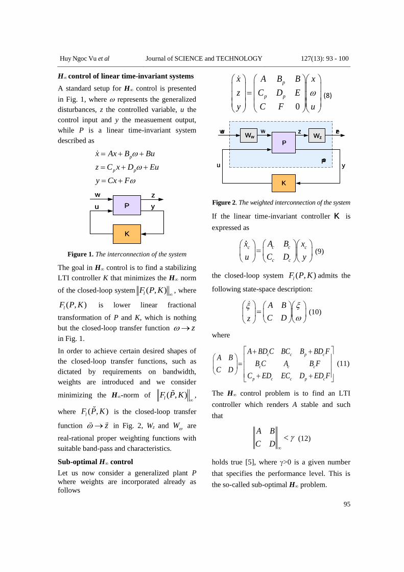
Huy Ngoc Vu et al Journal of SCIENCE and TECHNOLOGY 127(13): 93 - 100
95
H∞ control of linear time-invariant systems
A standard setup for H∞ control is presented
in Fig. 1, where represents the generalized
disturbances, z the controlled variable, u the
control input and y the measuement output,
while P is a linear time-invariant system
described as
p
p p
x Ax B Bu
z C x D Eu
y Cx F
PP
ww zz
KK
uu yy
Figure 1. The interconnection of the system
The goal in H∞ control is to find a stabilizing
LTI controller K that minimizes the H∞ norm
of the closed-loop system ( , )lF P K
, where
( , )lF P K is lower linear fractional
transformation of P and K, which is nothing
but the closed-loop transfer function z
in Fig. 1.
In order to achieve certain desired shapes of
the closed-loop transfer functions, such as
dictated by requirements on bandwidth,
weights are introduced and we consider
minimizing the H∞-norm of ( , )lF P K
,
where ( , )lF P K is the closed-loop transfer
function z in Fig. 2, Wz and W are
real-rational proper weighting functions with
suitable band-pass and characteristics.
Sub-optimal H∞ control
Let us now consider a generalized plant P
where weights are incorporated already as
follows
0
p
p p
x A B B x
z C D E
y C F u
(8)
PP
ww zz
KK
uu yy
WwWw WzWz
ezezewew
ePeP
Figure 2. The weighted interconnection of the system
If the linear time-invariant controller KK is
expressed as
c cc c
c c
A Bx x
C Du y
(9)
the closed-loop system ( , )lF P K admits the
following state-space description:
A B
C Dz
(10)
where
c c p c
c c c
p c c p c
A BD C BC B BD FA B
B C A B FC D
C ED EC D ED F
(11)
The H∞ control problem is to find an LTI
controller which renders A stable and such
that
A B
C D
(12)
holds true [5], where >0 is a given number
that specifies the performance level. This is
the so-called sub-optimal H∞ problem.
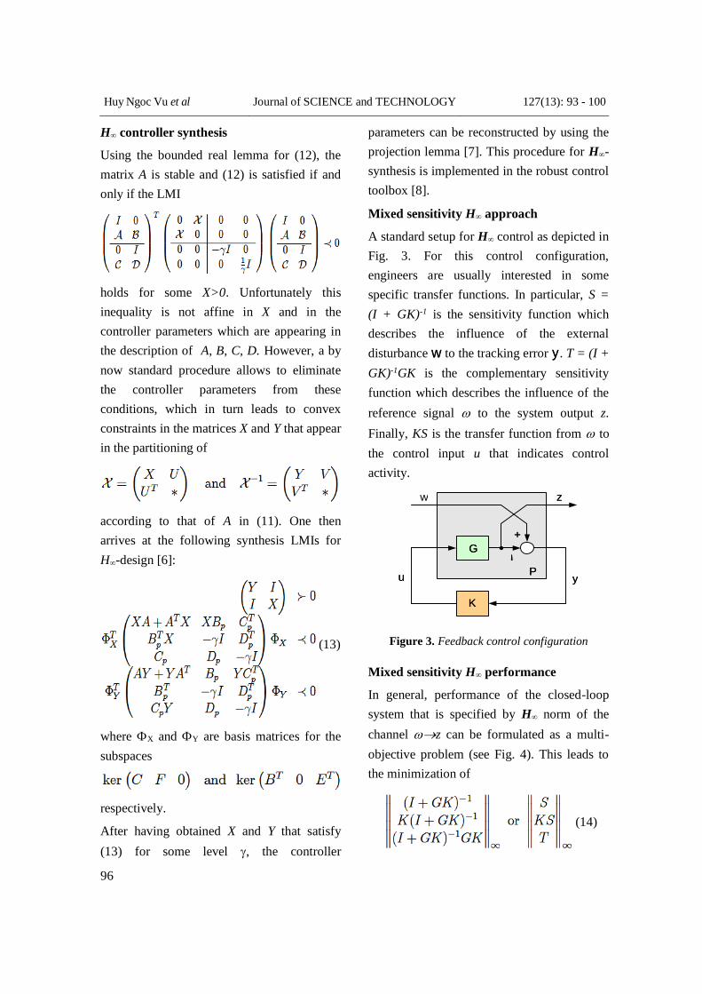
Huy Ngoc Vu et al Journal of SCIENCE and TECHNOLOGY 127(13): 93 - 100
96
H∞ controller synthesis
Using the bounded real lemma for (12), the
matrix A is stable and (12) is satisfied if and
only if the LMI
holds for some X>0. Unfortunately this
inequality is not affine in X and in the
controller parameters which are appearing in
the description of A, B, C, D. However, a by
now standard procedure allows to eliminate
the controller parameters from these
conditions, which in turn leads to convex
constraints in the matrices X and Y that appear
in the partitioning of
according to that of A in (11). One then
arrives at the following synthesis LMIs for
H∞-design [6]:
(13)
where X and Y are basis matrices for the
subspaces
respectively.
After having obtained X and Y that satisfy
(13) for some level , the controller
parameters can be reconstructed by using the
projection lemma [7]. This procedure for H∞-
synthesis is implemented in the robust control
toolbox [8].
Mixed sensitivity H∞ approach
A standard setup for H∞ control as depicted in
Fig. 3. For this control configuration,
engineers are usually interested in some
specific transfer functions. In particular, S =
(I + GK)-1 is the sensitivity function which
describes the influence of the external
disturbance ww to the tracking error yy. T = (I +
GK)-1GK is the complementary sensitivity
function which describes the influence of the
reference signal to the system output z.
Finally, KS is the transfer function from to
the control input u that indicates control
activity.
GG
uu
KK
yy
zzw
++
¡¡
PP
Figure 3. Feedback control configuration
Mixed sensitivity H∞ performance
In general, performance of the closed-loop
system that is specified by H∞ norm of the
channel z can be formulated as a multi-
objective problem (see Fig. 4). This leads to
the minimization of
(14)

Huy Ngoc Vu et al Journal of SCIENCE and TECHNOLOGY 127(13): 93 - 100
97
The multi-variable loop shaping with various
specifications (14) is the so-called the mixed
sensitivity H∞ design approach.
GGuu
KKyyw
++ ¡¡
z1z1
z2z2
z3z3
zz
Figure 4. Multi-objective problem
It is well-known in the literature that the
transfer functions S, T, and KS need to be
small in magnitude in order to achieve good
command tracking and robust stability.
However, the well-known constraint S+T=I
reveals that these requirements can not be
achieved simultaneously over the whole
frequency range. However, the use of
frequency filters or weighting functions opens
up the possibility to minimize the magnitudes
of S, T, and + over different frequency ranges.
Hence, in practice, instead of minimizing (14)
one rather determines a stabilizing LTI
controller K that minimizes the cost function
(15)
here WS, WP, WT are suitably chosen
weighting functions (Fig. 5).
GGuu
KKyyw
WTWT
WPWP
WSWS
++ ¡¡
zz
Figure 5. Mixed sensitivity H∞ control
DESIGNING AN H∞ CONTROLLER FOR
A DC MOTOR
Due to Ra, La, Km are uncertain parameters,
we can represent them as follow
0
0
0
(1 )
(1 )
(1 )
a a r r
a a l l
m m m m
R R
L L
K K
where Ra0, La0, Km0 are the nominal
parameters; r, l, m and -1 r, l, m 1
represent the variations of the system
parameters.
The model of the DC motor with uncertainties
is shown in Fig. 6.
RRvava
RR
- -
+
-
+
_x1_x1
_x2_x2
x1x1
x2x2
©©
2¼©2¼©
M rM r
±r±r
M lM l
±l±l
MmMm
±m±m
MmMm
±m±m
TLTL
urur
yryr
ununynyn
uiuiyiyi
ulul ylyl
vivi
vrvr
vnvn
9.55
J
Figure 6. The uncertain model
This model can be rearrange to the M ¢M ¢
configuration with matrix MM given by

Huy Ngoc Vu et al Journal of SCIENCE and TECHNOLOGY 127(13): 93 - 100
98
0 1 0 1
0 0 0 0 01
2 2 0 2 2
0 1 0 1
0 0 0 0 0
0
0
01
2
10 0
0 0 0 0 0
10 0
0 0 0 0 0 0 0
0 0 0 0 0 0 0
0 0 0 0 0 0 0
1 0 0 0 0 0 0 0
0 1 0 0 0 0 0 0
a m mrl
a a a a a
m m
l a m mrl
a a a a ar
an
mi
m
R K
L L L L Lx
x K
y R K
L L L L Ly
Ry
Ky
Ky
y
1
2
l
r
n
i
L
a
x
x
u
u
u
u
T
v
and the matrix is given by
i
n
r
l
m
m
r
l
i
n
r
l
y
y
y
y
u
u
u
u
000
000
000
000
=
The certain model of the DC motor can be
represented as in Fig. 7.
GmGm
ulul
urur
unun
vava
TLTL
ylyl
yryr
ynyn
yiyi
y1y1
uiui
y2y2
Figure 7. Certain model of the DC motor
SIMULATION RESULTS
Frequency response
100
101
102
103
104
105
106
-150
-100
-50
0
From: nref To: [+Gupss]
Magnitude (
dB
)
Closed-loop performance of reference inputs to outputs
Frequency (rad/s)
Figure 8. Output response with reference input
(speed)
100
101
102
103
104
105
106
-45
-40
-35
-30
-25
-20
-15
-10
-5
0
5
From: nref To: [+nref-Gupss]
Magnitude (
dB
)
Closed-loop performance of the load to outputs
Frequency (rad/s)
Figure 9. Reference input with error
100
101
102
103
104
105
106
-140
-130
-120
-110
-100
-90
-80
-70
-60
-50
From: TL To: [+Gupss]
Mag
nitu
de (
dB)
Closed-loop performance of reference inputs to outputs
Frequency (rad/s)
Figure 10. Effect of the load TL to output speed
100
101
102
103
104
105
-120
-100
-80
-60
-40
-20
0
20
40
From: nref To: [+Gupss]
Magnitude (
dB
)
Bode Diagram
Frequency (rad/s)
Figure 11. Output Response
100
101
102
103
104
-50
-40
-30
-20
-10
0
10
20
30
40
50
From: nref To: [+nref-Gupss]
Magnitu
de (
dB
)
Bode Diagram
Frequency (rad/s)
Figure 12. Error

Huy Ngoc Vu et al Journal of SCIENCE and TECHNOLOGY 127(13): 93 - 100
99
Time response
0 0.005 0.01 0.015 0.02 0.025 0.03 0.035 0.04 0.045 0.050
0.2
0.4
0.6
0.8
1
1.2
1.4Closed-loop performance of reference inputs to outputs
time (s)
Figure 13. Step response
0 0.005 0.01 0.015 0.02 0.025 0.03 0.035 0.04 0.045 0.05-0.2
0
0.2
0.4
0.6
0.8
1
1.2Closed-loop performance of reference inputs to control errors
time (s) Figure 14. Error
0 0.005 0.01 0.015 0.02 0.025 0.03 0.035 0.04 0.045 0.05-1.8
-1.6
-1.4
-1.2
-1
-0.8
-0.6
-0.4
-0.2
0x 10
-3 The effect of torque to output
time (s)
Figure 15. The effect of torque to output
0 0.005 0.01 0.015 0.02 0.025 0.03 0.035 0.04 0.045 0.050
0.2
0.4
0.6
0.8
1
1.2
1.4
1.6
1.8x 10
-3 The effect of torque to control errors
time (s)
Figure 16. The effect of torque to control errors
CONCLUSIONS
The paper presents an approach for the robust
controller design for the DC motor. The
approach is based on uncertain model of the
motor. Consequently the H1H1 controller was
designed via Matlab functions. The controller
is of the second order, thus quite simple. It
was tested in a simulation and it was proved
that the controller is able to stabilize the
system even the most degraded model within
the given uncertainty range. Such a controller
should be theoretically able to stabilize also
the real system with behavior covered by the
uncertainty. The approach is possibly
applicable to other systems where it is
impossible to create precise model for the
control design.
REFERENCES
1. Dayang. F. B, “Control of DC motor using PI
controller”, Thesis, 2005.
2. Mohammed S.Z, “Parameters identification of
a permanent magnet DC motor”, Master thesis,
2009.
3. K. Zhou and P. P. Khargonekar. An algebraic
riccati equation approach to H1H1 optimization.
Systems and Control Letters, 11:85–91, 1988.
4. J. G. Van Antwerp and R. D. Braatz. A tutorial
on linear and bilinear matrix inequalities. Journal
of Process Control, 10:363–385, 2000.
5. P. Apkarian and P. Gahinet. A convex
characterization of gain-scheduled H1H1
controllers. IEEE Transactions on Automatic
Control, 40:853–864, 1995
6. C. W. Scherer. Mixed H2/H1H1 control for time-
varying and linear parametrically-varying systems.
International Journal of Robust and Non-linear
Control, 6:929 – 952, 1996.
7. C. W. Scherer and S.Weiland. Linear Matrix
Inequalities in Control. Lecture notes in DISC
course, 2005.
8. A. Packard M. Safonov G. Balas, R. Chiang.
Robust control toolbox for use with Matlab,
volume 3. The MathWorks, 2005.

Huy Ngoc Vu et al Journal of SCIENCE and TECHNOLOGY 127(13): 93 - 100
100
TÓM TẮT
ĐIỀU KHIỂN BỀN VỮNG ĐỘNG CƠ MỘT CHIỀU
Vũ Ngọc Huy*, Trần Mạnh Tuấn, Nguyễn Thị Mai Hương, Nguyễn Tiến Hưng
Trường Đại học Kỹ thuật Công nghiệp – ĐH Thái Nguyên
Các động cơ DC được sử dụng trong rất nhiều ứng dụng trong cuộc sống, giải phóng sức lao động
của con người trong nhiều công việc. Tuy nhiên, vẫn còn khó khăn trong việc thiết kế một hệ
thống điều khiển cho động cơ DC bởi vì dữ liệu được sử dụng để thiết kế bộ điều khiển không phù
hợp với dữ liệu đo được trong thực tế. Điều này là do các thông số động cơ thường thay đổi theo
thời gian. Do đó bộ điều khiển không thể bảo đảm thực hiện hoàn hảo để có hiệu suất cao nhất.
Trong nghiên cứu này, các thông số của động cơ được xác định bằng cách sử dụng phần mềm
Matlab. Sau đó một bộ điều khiển H∞ được thiết kế để đảm bảo rằng hiệu suất của hệ thống được
điều khiển được duy trì với những thay đổi của các thông số động cơ trong một dải xác định. Các
kết quả nghiên cứu được đưa ra bởi các kết quả mô phỏng trong môi trường Matlab / Simulink.
Từ khóa: Động cơ DC, tham số bất định, H-vô cùng, hiệu suất.
* Tel: 0983169582; Email: [email protected]

Kien Ngoc Vu et al Journal of SCIENCE and TECHNOLOGY 127(13): 101 - 106
101
MODEL REDUCTION IN SCHUR BASIS WITH POLE RETENTION
Kien Ngoc Vu1,*, Du Huy Dao1, Cong Huu Nguyen2
1University of Technology – TNU; 2Thai Nguyen University ABSTRACT
Model order reduction is a research direction which is more interested scientists in recent years.
There have been many order reduction algorithm introduced to many different approaches in
which retaining the important poles of the original system in the reduced root system is the right
approach and has many advantages.
This paper presents a new model order reduction algorithm, the order reduction algorithm based on
Schur analysis, based on the idea of keeping the important poles of the original system in the order
reduction process. This algorithm transforms matrix A of the higher-order original system to upper
- triangle matrix on which the poles are arranged in descending important properties on the main
diagonal of the upper – triangle matrix. The illustrative examples show the correctness of the
model order algorithm.
Keywordss: Model order reduction, Schur analysis, important poles.
INTRODUCTION*
In the previous paper [1] the authors
introduce balanced truncation algorithms. The truncation [1] for the system is based on
Hankel singular value (It removes the state corresponding to Hankel small singular
values) leading to important climax points of the root system without conserved reduced
order system. However, important climax poles (dominant poles) are invariant in the
real system, so it should be preserved in process of order reduction. Therefore, this
paper, we introduce a new algorithm, the order reduction algorithm based on Schur
analysis, based on the idea of keeping the important poles of the original system in the
order reduction process. The illustrative examples shows the correctness of the model
order algorithm.
MODEL ORDER REDUCTION ALGORITHM
Problem of order reduction model
A linear system is given with continuous-time
constant parameters available multiple-inputs multiple-outputs described in state space by
the following equations:
x=Ax+Bu
y=Cx(1)
* Tel: 0965869293; Email: [email protected]
In which, x Rn, u Rp, y Rq, A Rnxn, B
Rnxp, C Rqxn.
The goal of the order reduction problem with
model described by (1) is to find models
described by systems of equations:
r r r r
r r r
x =A x +B u
y =C x(2)
In which, xr Rr, u Rp, yrRq, Ar Rrxr, Br
Rrxp, Cr Rqxr, với r n;
So that the model described by (2) can be
replaced by the model described in (1) to
apply in analysis, design and control system.
Model reduction in Schur basis with pole
retention
Model reduction in Schur basis with pole
retention was developed by the researched
team based on truncation technique and
analysis of Schur.
Truncation technique is a method of simple
order reduction. In which, the main idea of it
can be divided into 2 steps: the step 1 is to
convert the high original system to the
equivalent system with a non-singular
transformation in state space. The step 2 is to
delete rows and columns of similar systems to
generate the reduced order system. The two
most typical algorithms for truncation

Kien Ngoc Vu et al Journal of SCIENCE and TECHNOLOGY 127(13): 101 - 106
102
technique are balanced truncation [1] and
model truncation [2] in many disorders.
However, disadvantages of both methods are
the use of the Singular Value Decomposition
(SVD) which required a lot of bidding
conditions. On the other hand, the truncation
for the system is based on Hankel singular
value (It removes the state corresponding to
Hankel small singular values) leading to
important climax points of the root system
without conserved reduced order system.
Important climax poles (dominant poles) are
invariant in the real system, so it should be
preserved in process of order reduction.
From those disadvantages, the key idea of
algorithm provided by the author, Minh H.B
and his research group [3] is to convert the
matrix A of the internal system to (1) of the
triangular matrix based on Schur analysis
(without SVD analysis), on the basis the poles
are arranged in descending important
properties on the main diagonal of the upper
triangular matrix A. Then go to the step 2 of
the truncation technique, which helps
important climax poles (dominant poles) to be
preserved in the reduced order system.
Order reduction algorithm is as following
Algorithm 2.2.1 (Triangle realization)
Assume that the linear time-invariant system
(A, B, C, D) is asymptotically stable and in a
minimal representation.
Input: The original system (A, B, C, D)
Step 1: Compute observability Grammians
Q from Lyapunov equation A*Q + QA +C*C = 0
Step 2: Compute Cholesky factorization
Q = R*R.
Step 3: Compute Schur decomposition of
RAR-1:
RAR-1=UU*, where U is unitary matrix and
is upper triangle matrix.
Step 4: Compute non-singular
transformation T = R−1U
Step 5: Compute A, B, C, D = (T-
1AT, T-1B, CT,D)
Output: An equivalent system with realization
A, B, C, D
The output realization in Algorithm 2.2.1 is
said to be triangle realization.
Algorithm 2.2.2 (Re-ordering the poles by
dominance index)
Input: Triangle realization A, B, C, D ,
which is the output of Algorithm 2.2.1
Step 1: For each pole i, i = 1 … n, compute
its dominance index i i
2
i
i
C BR =
Reλ.
Step 2: Choose the largest dominance index 1i
R
Step 3: Reorder pole 1i
λ (and its conjugate
1iλ , if it appears) to the first position in the
diagonal of A by unitary matrix U1:
Comment of Step 3: Algorithms for
reordering eigenvalues in Schur
decomposition are referred to [7, 8]. It can be
done, for example, by MATLAB function
ordschur
Step 4: Compute new equivalent realization
(* *
1 1 1 1U AU , U B, CU ).
Step 5: Remove two first rows and columns
of (* *
1 1 1 1U AU , U B, CU ) to obtain a smaller
realization ( ˆ ˆˆA, B, C ) with (n − 2)
dimensions.
Step 6: Do the same procedure from Step 1 to
Step 5 for smaller realization ( ˆ ˆˆA, B, C ) and
continue this loop until all poles are re-
ordered.

Kien Ngoc Vu et al Journal of SCIENCE and TECHNOLOGY 127(13): 101 - 106
103
THE ILLUSTRATIVE EXAMPLES
Reducing higher-order controller
H full order controller of the robot balanced
system [4] has the following transfer function
model: 6 5 4
3 2
8 7 6 5 4 4
3 2 5
0.1209 0.01874 27.07
2.077 1505 6.713 2853( )
0.3542 390 50.7 3.53
936.7 4.674 786.2 1.472
s s s
s s sW s
s s s s e s
s s s e
(3)
The full order controller 6th-order will lead to
many disadvantages when we perform robot
balanced control programs due to complex
program that make increase of processing
time, the slow speed of response of the
control system, without a good response to
real-time requirements of the controller and
instability of balanced system. So, in order to
improve the quality of this controller, it
should implement reduced order controller to
let program code be simpler, reduction of
processing time, increase of response speed,
but still satisfy requirements of sustainable
stability of the system.
Implementation of reduced order H control
algorithm reduced sufficient steps mentioned
above; we obtain the following result table:
Table 1. Results of the order reduction controller
of the robot balanced system
Order Transfer function – Wcr(s)
5
4 3 2
5 4 3 2
1275 8.694 5 4.367 5
1.359 8 1.209 7
715.6 2.349 4 2.768 5
3.777 6 3.183 5
s e s e s
e s e
s s e s e s
e s e
4 9.46655409.39787.33
4773.15993.11.3481275234
23
ssss
esess
3 550639578.33
5993.18.234127523
2
sss
ess
2 43.9425.30
6.24711302
ss
s
1 71.26
1006
s
Evaluation of the reduced order error based
on H norm, we obtain the following result
table.
Table 2. Error between the 6th-order controller
and reduced order controller
Order Error
Hcr ss )(W)(Wc
5 5.1995e-005
4 4.3560e-004
3 1.7910
2 37.2364
1 38.1419
To verify the reduced order model, the
researchers have simulated the excessive
response of the full order controller and
reduced order controllers. The simulation
results in Matlab/Simulink as shown in Fig 1.
Figure 1. Results of simulation of full order
controller and reduced order controller
To compare the effectiveness of the new
order model reduction algorithm with the
algorithm based on Schur analysis of M. G.
Safonov and R. Y. Chiang [5], the authors
perform reduced order controller (3) using
algorithm in [5], we obtain the results in the
following table 3.
Evaluation of the reduced order error based
on H norm, we obtain the following result
table 4.

Kien Ngoc Vu et al Journal of SCIENCE and TECHNOLOGY 127(13): 101 - 106
104
Table 3. Results of the reduced order controller
using algorithm in [5]
Order Transfer function – Wcr(s)
5
3 2
5 4 2
4
3
.694 005 4.366 005
1.359 008 1.209 007
715.6 2.349 004 2.768 005
3.777 006 3.183 005
1275 8 e s e s
e s e
s s e s e s
e s
s
e
4 3 2
4 3 2
1275 348.2 1.993 005 1.775 004
33.87 397.9 5540 467.2
s s e s e
s s s s
3 2
3 2
1275 233.8 1.992 005
33.76 395 5499
s s e
s s s
2 2
946.3 s + 227.9
24.55 386s s
1 946.4
s + 24.55
Table 4. Error between the 6th-order controller
and reduced order controllers
Order Error
Hcr ss )(W)(Wc
5 1.5977e-006
4 3.4723e-004
3 1.7678
2 37.3971
1 38.8756
From the result of order reduction according
to two methods we see: Compared to
response h(t) of the full 6th-order controller,
the response h(t) of the 5th, 4th-order reduction
controller coincide completely; response h(t)
of the 3rd-order reduction controller has very
small differences; response h(t) of 2nd and 1st-
order reduction controllers, has greater
differences. Therefore we can use the 5th, 4th
and 3rd-order reduction controller to replace
the full 6th orders controller.
Comparison of the poles between 6th-order
controller and the 3rd-order reduction
controller, we obtain the result as follows:
+ Poles of 6th-order original controller
-681.74; -26.71; -3.5353 + 13.9156i; -3.5353;
- 13.9156i; -0.09; -0.08
+ Poles of 3rd-order reduction controller using
algorithm in [5]: -26.6843; -3.5396 +13.912i;
-3.5396 -13.912i
+ Poles of 3rd-order reduction using new
algorithm: -26.71; -3.5353 +13.9156i; -3.5353
-13.9156i
The important pole of the original 6th-order
controller has been preserved in the 3rd-order
reduction system using new algorithm, with
algorithm of M. G. Safonov and R. Y. Chiang
[5], the important pole of the original 6th-
order controller is not conserved in the 3rd-
order reduction system.
Reducing 8th–order SISO system
A 8th–order SISO system often is selected to
evaluate and compare between the model
order reduction algorithm is given in [6] as
follows:
( )( )
( )
N sW s
D s (5)
with: N(s) = 0.1209s6 + 0.01874s5 + 27.07s4 +
2.077s3 + 1505s2 + 6.713s + 2853
D(s) = s8 + 0.3542s7 + 390s6 + 50.7s5 +
5.53e4s4 + 936.7s3 + 4.674s2 + 786.2s +
1.472e5
Simplification of the model system will help
the process of understanding the system
easier. The authors perform reduced order
model system based on Schur analysis, the
results shown as follows:
Table 5. Results of the order reduction of the 8th-
order SISO system
Order Transfer function – Wcr(s)
7
6 5 4
3 2
7 6 5 4
3 2
0.0001106 0.1184 0.05018
13.12 0.6966 25.44 0.4283
0.3436 278.1 10.46
4162 50.89 1314 13.93
s s s
s s s
s s s s
s s s
6
5 5 4 3
2
6 5 4 3
2
1.011 0.1185 0.01536
13.12 0.05516 25.44
0.333 278 7.516
4162 6.772 1314
e s s s
s s
s s s s
s s
5 4 3 2
5 4 3 2
0.004671 0.1116 1.317 11.57 19.14
0.3324 277.7 7.256 4072 2.24
s s s s
s s s s s

Kien Ngoc Vu et al Journal of SCIENCE and TECHNOLOGY 127(13): 101 - 106
105
Order Transfer function – Wcr(s)
4
6 3 2 5
4 3 2
5.755 0.04525 9.796 0.09565
0.009 15.85 0.01963 5.012
e s s e s
s s s s
3
2
3 2
0.004693 0.03988 0.07292
0.00845 15.53 0.008542
s s
s s s
2
6
2
6.438 0.005329
0.0011 0.3227
e s
s s
1 0.004694
0.00055s
Evaluation of the reduced order error based
on H norm, we obtain the following result
table 6.
Table 6. Error between the 8th-order SISO system
and reduced order systems
Order Error ( ) ( )rW s W s
7 0.0114
6 0.0109
5 8.5286
4 0.0140
3 8.5199
2 1.2822
1 8.5199
Bode plots of the original system, reducted
order systems are shown Fig.2
Figure 2. Bode plots of the original system,
reduced order systems
From the result of order reduction, evaluation of the reduced order error and bode plots, we see: the error between the original 8th-order SISO system and the 7th, 6th and 4th-order reduction system is very small; the error
between the original 8th-order SISO system and the 5th, 3rd, 2nd and 1tst-order reduction system is very big. Therefore we can use the 7th, 6th and 4th-order reduction system to replace the 8th-order SISO system.
The authors perform order reduction of 8th-
order SISO system using the algorithm of M.
G. Safonov and R. Y. Chiang [5], we obtain
the results in the following table:
Table 7. Results of the order reduction of the 8th-
order SISO system
Oder Tranfer function Wr(s)
7
6 5 4
3 2
7 6 5 4
3 2
0.0001204 0.1182 0.05242
13.11 0.7416 25.44 0.4662
0.3432 278 10.75
4162 55.5 1314 15.39
s s s
s s s
s s s s
s s s
6
5 4 3
2
6 5 4 3
2
1.15 005 0.1185 0.01582
13.12 0.0555 25.43
0.3332 277.9 7.518
4160 6.77 1313
e s s s
s s
s s s s
s s
5
4 3
2
5 4 3
2
0.002274 0.04519
0.04324 0.09553 0.02669
0.1695 15.86
2.564 5.015 0.8044
s s
s s
s s s
s s
4
3 2
4 3 2
1.148 005 0.04525
0.0001099 0.09565
0.009 15.85
0.01963 5.012
e s s
s
s s s
s
3 2
3 2
0.005077 0.005312 0.001657
0.005046 0.3227 0.001275
s s
s s s
2 2
1.289e-005 s + 0.0053
0.0011 0.3227
29
s s
1 0.004697
s + 0.0005502
Evaluation of the reduced order error based
on H norm, we obtain the following result
table 8.
From the result of order reduction, evaluation
of the reduced order error, we see: the error
between the original 8th-order SISO system
and the 7th, 5th, 6th and 4th-order reduction

Kien Ngoc Vu et al Journal of SCIENCE and TECHNOLOGY 127(13): 101 - 106
106
system is very small; the error between the
original 8th-order SISO system and the 3rd, 2nd
and 1tst-order reduction system is very big.
Therefore we can use the 7th, 6th, 5th and 4th-
order reduction system to replace the 8th-order
SISO system.
Table 8. Error between the 8th-order SISO system
and reduced order system
Order Error ( ) ( )rW s W s
7 0.0109
6 0.0109
5 0.0138
4 0.0140
3 1.2809
2 1.2822
1 8.5199
Thus reduced order results according to model order reduction algorithm based on analysis Schur are complete correct.
CONCLUSIONS
This paper introduces detailed order model reduction algorithms based on Schur analysis. The most important new feature of the algorithm is the ability to arrange the poles in the importance of decreasing on the main diagonal of the upper triangular matrix A and the ability to retain the important pole of the original model in order reduction model. The illustrative examples show the correctness of the model order algorithm.
REFERENCES
Cong N.H , Kien V.N , Du D.H , Research reduce
order model algorithm by balancing method,
Journal of Science and Technology of the Technical
University, Vol 80, pp. 34-39, 2011
A.C Antoulas, Approximation of Large – Scale
Dynamical Systems, SIAM, 2005.
Minh H.B and Kiyotsuga Takaba.(2011) “Model
reduction in Schur basic with pole retention and H
- norm error bound,” In: Proceedings of
international workshop on Modeling, Systems, and
Conrol 2011
Thanh B.T, and Manukid Parnichkun. (2008)
“Balancing control of Bicyrobo by particle swarm
optimization – based structure-specified mixed
H2/H control,” International Journal of Advanced
Robotic Systems 2008; 5(4): 395- 402.
M. G. Safonov and R. Y. Chiang, "A Schur Method
for Balanced Model Reduction," IEEE Trans. on
Automat. Contr., vol. 34, no. 7, July 1989, pp. 729-
733.
J. Rommes, Methods for eigenvalue problems with
applications in model order reduction, PhD thesis,
Utrecht University, 2007
Zhaojun Bai, J.W. Demmel, On swapping diagonal
blocks in real Schur form, Linear Algebra and its
Applications, Vol. 186, pp. 755, 1993.
D. Kressner, Block algorithms for reordering
standard and generalized Schur forms, ACM
Transactions on Mathematical Software, Vol. 32,
No. 4, pp. 521-532, 2006.
TÓM TẮT
THUẬT TOÁN GIẢM BẬC BẢO TOÀN ĐIỂM CỰC
DỰA TRÊN PHÂN TÍCH SCHUR Vũ Ngọc Kiên1,*, Đào Huy Du1, Nguyễn Hữu Công2
1Trường Đại học Kỹ thuật Công nghiệp – ĐH Thái Nguyên; 2Đại học Thái Nguyên
Giảm bậc mô hình là một hướng nghiên cứu đang được nhiều nhà khoa học quan tâm trong những
năm gần. Đã có rất nhiều thuật toán giảm bậc được giới thiệu với nhiều hướng tiếp cận khác nhau
trong đó bảo lưu các điểm cực quan trọng của hệ gốc trong hệ giảm bậc là một hướng tiếp cận đúng
đắn và có nhiều ưu điểm.
Bài báo giới thiệu một thuật toán giảm bậc mô hình mới, thuật toán giảm bậc dựa theo phân tích
Schur, dựa trên ý tưởng bảo lưu các điểm cực quan trọng của hệ gốc trong quá trình giảm bậc. Thuật
toán mới chuyển đổi ma trận A của hệ gốc bậc cao về dạng ma trận tam giác trên trong đó các điểm
cực được sắp xếp theo tính chất quan trọng giảm dần trên đường chéo chính của ma trận tam giác
trên. Các ví dụ minh họa thể hiện tính đúng đắn của thuật toán giảm bậc
Từ khoá: Giảm bậc mô hình, thuật toán Schur, điểm cực quan trọng.
* Tel: 0965869293; Email: [email protected]

Viet Quoc Vu Journal of SCIENCE and TECHNOLOGY 127(13): 107 - 110
107
IMPROVING THE EFFICIENCY OF CONVENTIONAL DRINKING-WATER-
TREATMENT PROCESSES IN THE REMOVAL OF ARSENIC
Viet Quoc Vu*
University of Technology - TNU
ABSTRACT Since Vietnam is one of the most rice producing countries in the world, a huge amount of rice hull
waste produced every year has been raising environmentally significant concerns. This study aims
to build a model of improving the efficiency of the treatment process of removing arsenic from
drinking water using activated carbon derived from rice hull. In this model, the efficiencyof
treatment process is optimized due to the combination of the advantages of iron and activated
carbon. The iron hydroxide phases can improve maximum adsorption capacity and the activated
carbon can offer a high surface area for adsorption.
Keywordss: Drinking-water-treatment, removing arsenic, rice hull, activated carbon.
INTRODUCTION
Arsenic contamination has been a
considerable concern in many areas in
Vietnam. Arsenic element existing in nature
as As(III) and As(V). It is important to
remove both species of arsenic from drinking
water. Many studies have been conducted to
produce activated carbon from rice hulls for
arsenic removal. However, the arsenic
removal rate of activated carbon is not high
enough to fulfill health standards.
The most common process used to produce
activated carbon is chemical process. During
this process, carbonization and activation
occur at the same time. A chemical
(dehydrating) agent such as zinc chloride is
used to decompose the cellulose of rice hull.
An issue during this process is thatthe
efficiency of the removing metal irons is still
limited. This study aims to improve
performance of activated carbon, in order to
improve the efficiency of the removing
arsenic irons from drinking water.
2A model of improving the efficiency of the
removing arsenic from drinking water
process
This process combines the advantages of
both, iron and activated carbon. The Iron
hydroxide phases increase the adsorption
capacity. Activated carbon can offer a high
surface area for adsorption.
Figure 1. Iron-impregnated activated carbon process for removing Arsenic irons*
* Tel: 0943952708; Email: [email protected]

Viet Quoc Vu Journal of SCIENCE and TECHNOLOGY 127(13): 107 - 110
108
Table 1. The description of producing Iron-impregnated activated carbon for removing Arsenic irons
Description Temperature Time Equipment
Step 1 Washing 100g Rice Hull RC Deionized water
Step 2 Drying 80°C 5 hours Furnace
Step 3 Mixing with 1.0 M NaOH solution RC 10 hours 40g NaOH,
1 L Deionized water
Step 4 Washing until the base is undetected in
the filtrate RC Deionized water
Step 5 Drying until constant weight 80°C Furnace
Step 6 Grinding and sieving RC Siever and Grinder
Step 7
Covering with aluminum foil, placing
in alumina crucible, capping with an
alumina cover
RC aluminum foil, alumina
crucible with lid
Step 8 Placing in furnace 800°C 2 hours Furnace
Step 9 Cooling RC
Step 10 Rinsing three times in deionized water RC Deionized water
Step 11 Drying Furnace 110°C 10 hours Furnace
Step 12 Cooling RC
Step 13
FeCl2 (5.5g) is dissolved in 100ml
deionized water. Adding NaOH to
ferrous chloride solution until pH 12
RC
5.5g FeCl2,
100 ml Deionized
water, NaOH
Step 14 Adding AC (30g) to solution without
headspace RC
Glass bottle with lid,
250ml
Step 15 Shaking 24 hours Rotator
Step 16 Filtered Filter Bag
Step 17 Drying 110°C 10 hours Furnace
Step 18 Cooling RC
Step 19 Mix Fe-AC with 1M NaOH for 24
hours RC 24 hours
40g NaOH
1L Deionized water
Step 20 Soaking RC 24 hours 100 ml 38% HCl
Step 21 Washing and Drying RC Deionized water
RC: Room temperature

Viet Quoc Vu Journal of SCIENCE and TECHNOLOGY 127(13): 107 - 110
109
DISCUSSION
Choosing chemical agent NaOH
In this process,the silica in the rice hulls
reacts with NaOH forming sodium silicate
which leads to a porous surface area. Using
NaOH as a chemical agent results in a
comparable low surface area with a big pore
volume. It is used here for two reasons.
Firstly,Qiganget al. [1] state in their report
that the best results of coating activated
carbon with iron take place using a macro
pore activated carbon which means a low
surface area and a large pore volume. This is
because the large pores Fe3+ can enter deep
into the activated carbon. Using activated
carbon with small pores leads to an
impregnation only on the surface of activated
carbon. Secondly using NaOH will simplify
the process since it is also used for further
steps. The impact of NaOH on rice hulls is
shown in the picture stated below.
Choosing impregnation with Fe2+
In this process impregnation with Fe2+ is
chosen. Iron forms an amorphous layer of
iron oxides on the activated carbon surface.
Due to this layer the net positive surface
charge of the activated carbon is increased
and therefore the arsenic removal capacity of
activated carbon is enhanced. Arsenic
adsorption to iron oxide-hydroxide surfaces
can be described by the ligand exchange
mechanism. In the adsorption process,
arsenic species can replace hydroxyl ion
(OH-) on the surfaces of iron oxide-
hydroxides, forming inner-sphere complexes
[3]. Furthermore ferrous is soluble at a wide
range of pH and can diffuse deep into the
internal pores of the activated carbon. The
degree of impregnation onto the activated
carbon surface is maximal when the net
charge of the activated carbon surface
becomes negative. The net surface charge is
highly dependent on the pH. Therefore the pH
of the ferrous solution is increased to pH 12
by adding NaOH.
CONCLUSION
The removal rates of toxic metals have been
very promising and with adaptions like
iron-impregnation the results can be even
improved. The model of the process to
produce iron-impregnated activated carbon
for arsenic removal is a combination of a
variety of processes and could improve
the arsenic removal rate of activated carbon,
in which iron hydroxide phases increase the
adsorption capacity and activated carbon offer
a high surface area for adsorption.
Figure 2. Impact of NaOH on rice hulls; (a) Raw rice hulls and (b) Rice hull treated with NaOH
(Adapted from [2])

Viet Quoc Vu Journal of SCIENCE and TECHNOLOGY 127(13): 107 - 110
110
REFERENCES
1. Qigang Chang et al. (2010, June). The
preparation of iron-impregnated granular activated
carbon for arsenic removal from water. Journal of
Hazardous Materials 184 2010, 515-522.
2. Mohd F. Taha et al. (2011). Removal of Ni(II),
Zn(II) and Pb(II) ions from Single Metal Aqueous
Solution using Activated Carbon Prepared from
Rice Husk. World Academy of Science,
Engineering and Technology 60 2011, 291-296.
3. HyonChong, Kim et al. (2009). Arsenic
removal from water using iron-impregnated
granularactivated carbon in presence of
bacteria. Journal of Environmental Science and
Health, Vol. 40 2010, 177-182.
4. Http://www.epa.gov/nrmrl/wswrd/dw/arsenic/
pubs/FundamentalsofAdsorptionforArsenicRemov
alfrom Water.pdf, 17.12.2013.
TÓM TẮT
NÂNG CAO HIỆU QUẢ QUÁ TRÌNH LOẠI BỎ THẠCH TÍN
TRONG NƯỚC SINH HOẠT
Vũ Quốc Việt*
Trường Đại học Kỹ thuật Công nghiệp – ĐH Thái Nguyên
Việt Nam là một trong những nước sản xuất gạo nhiều nhất trên thế giới, vì vậy một lượng lớn vỏ
trấu được tạo ra trong quá trình sản xuất gạo có thể gây ảnh hưởng đến các vấn đề về môi trường.
Việc tận dụng nguồn vỏ trấu cho các ứng dụng hữu ích đang là vấn đề được quan tâm lớn. Mục
tiêu của bài báo này là xây dựng một mô hình nâng cao hiệu quả của quá trình loại bỏ thạch tín
trong nước sinh hoạt bằng than hoạt tính được tạo thành từ vỏ trấu. Trong nghiên cứu này, hiệu
quả tối ưu của quá trình xử lý đạt được nhờ sự kết hợp ion sắt và than hoạt tính. Ion sắt nâng cao
tối đa hiệu quả hấp thụ thạch tín, trong khí đó than hoạt tính được hình thành với lượng lớn diện
tích bề mặt hấp thụ.
Từ khóa: Xử lý nước uống, loại bỏ thạch tín, vỏ trấu, than hoạt tính.
* Tel: 0943952708; Email: [email protected]

Huyen Vu Xuan Dang et al Journal of SCIENCE and TECHNOLOGY 127(13): 111 - 115
111
ASSESSMENT OF TREATED LATEX WASTEWATER REUSE FOR
PERENNIAL TREE IRRIGATION ON GROUND WATER QUALITY
Huyen Vu Xuan Dang1,*, Hanh Vu Bich Dang1,
Amira Abdelrasoul2, Huu Doan2, Dan Phuoc Nguyen1 1Hochiminh city University of Technology, VNU-HCM, Vietnam
2Ryerson University, Toronto, Canada
ABSTRACT
The study aimed to assess nutrient contamination to aquifer from reuse of latex wastewater for
perennial tree irrigation. The latex wastewater contains high nitrogen concentrations and BOD that
are required high treatment costs to meet Vietnam Industrial effluent standards. The reuse of
secondary treated effluent for rubber tree irrigation may be a potential benefit in terms of treatment
cost reduction as well as nutrient reuse.
A pilot experiment was done in two lots of 100 rubber trees each. The area of each lot was 7m x
2.5m. One lot was controlled without irrigation. The used irrigation water was taken from effluent
of a facultative waste stabilization pond of latex processing industry. Hydraulic rate, nutrient
loading and COD loading applied to the lot were 8m3/ha/week, 12.5 kgN/ha/day and 0.5 kg COD
/ha/day respectively.
GMS modeling was used for assessing nitrogen and COD transport in the aquifer. The first order
reaction modeling was used for biological conversion of COD and nitrogen during the infiltration
in the vadose layer. The results shown that transport of total nitrogen and COD in the ground water
were reached stable levels at 2 meter depth after 10 months and 10 meter after 12 months of
irrigation. In addition, scanning electron microscopy (SEM) images used to compare the soil
quality among the sites.
Keywords: Latex processing wastewater, nutrient reuse, Vietnam Industrial effluent standards,
Groundwater Modeling System (GMS), scanning electron microscopy (SEM).
INTRODUCTION*
Vietnam Rubber Group reported that the
rubber industry emits by 10 million cubic
meters of wastewater annually [1]. The latex
wastewater contains high organic and high
nitrogen (COD: 1,000 ÷ 10,000 mg/l, BOD5:
1,700 ÷ 9,000 mg/l and total nitrogen: 45 ÷
1,600 mg/l) [2]. To meet Vietnam Industrial
effluent standards, the reuse of secondary
treated effluent for rubber tree irrigation may
be a potential benefit in terms of treatment
cost reduction as well as nutrient reuse. Due
to high nutrient composition, orientation to
reuse wastewater after aerobic biological
treatment for irrigation combining with higher
processing soil treatment may reduce costs of
chemical and electricity. In addition, reuse of
nutrient compositions (nitrogen, phosphorous,
potassium) may decrease the amount of
* Tel: 0913179886; Email: [email protected]
chemical fertilizers and improve soil quality
by providing useful microorganisms and
humus after aerobic biological treatment. The
study aimed to assess nutrient contamination
to aquifer from reuse of latex wastewater for
perennial tree irrigation.
MATERIALS AND METHODS
Experimental site
The experiment was conducted at the Rubber
Research Institute of Vietnam (RRIV) in Ben
Cat District, Binh Duong province, Vietnam.
A pilot experiment (Figure 1) was done in
two lots of 100 rubber trees each. The
distance between rubber tree of each lot was
7m x 2.5m. Lot 0 (L0) was controlled without
irrigation. Lot 1 (L1) was watered by latex
wastewater after anaerobic stage with 20 liters
per rubber tree. Two observation wells about
18-20 meters in depth were drilled in the two
lots L0, L1.

Huyen Vu Xuan Dang et al Journal of SCIENCE and TECHNOLOGY 127(13): 111 - 115
112
X X X X X X . . . X X X X X X L0: without
irrigation 7m
X X X X X X . . . X X X X X X
X X X X X X . . . X X X X X X L1: watering
with treated
latex wastewater 7m
X X X X X X . . . X X X X X X
Rubber
trees Well 1 Well 0
Figure 1. Pilot scale irrigation experiment
The used irrigation water was taken from
effluent of a facultative waste stabilization
pond of latex processing industry. Hydraulic
rate, nutrient loading and COD loading
applied to the lot were 8m3/ha/week, 12.5
kgN/ha/day and 0.5 kg COD /ha/day
respectively.
Sampling and testing quality of the
wastewater
Treated wastewater was irrigated on every
Thursdays, from 08:00am during 1-2 hours.
Irrigation flow at each rubber’s root was
controlled by a counter clock to ensure 20
liters in every 12-14 seconds per rubber tree,
or equal to 10 m3 per ha per week. The
experiment was conducted in 16 weeks.
Water samples from the 2 observation wells
were taken by water pumps and then brought
to the laboratory for analyzing pH, COD,
TKN, N-NH4, N-NO3 and P - PO4.
Table 1. Characteristics of latex wastewater after
anaerobic pond
No Latex
wastewater
Average
concentration
1 pH 6.77
2 COD (mg/L) 407
3 TKN (mg/L) 176
4 NH3 – N (mg/L) 157
5 PO4 – P (mg/L) 282
Table 2. Modeling of latex wastewater
Type of
stream,
(i)
Latex wastewater (CS)
Latex
wastewater
of
anaerobic
pond
Anaerobic
effluent
Effluent of
facultative/
secondary
treatment
lt kk hk
COD (j),
mg/L 1000 500 250
TKN (k),
mg/L 500 150 60
Irrigation
load TL
(n)
Irrigation load m3/ha/day
30
50
80
120
Note: (i) – Type of wastewater: bi, kk, hk; (j) – COD: 1000, 500, 250 mg/L; (n) – 30, 50, 80, 120 m3/ha/day
Soil sampling and analyzing
Surface soil were sampled for SEM analysing at two sites: i) Inside the lot L0, soil were taken from the top, at 35cm depth and then mixed for one sample named D3; and ii) Inside the lot L1, soil were taken from the top, at 25cm depth and then mixed for one sample named CS3. SEM images at magnification 100 and 1,000 were conducted at the Innovation lab, Ryerson University, Toronto, Canada.
Input data for Groundwater Modeling System (GMS)
Irrigation load calculation option (n) 30, 50, 80 and 120 m3/ha/day, the results of the water analysis by the software MODFLOW with input data showned in the Table 2.

Huyen Vu Xuan Dang et al Journal of SCIENCE and TECHNOLOGY 127(13): 111 - 115
113
RESULTS AND DISCUSSIONS
Pilot scale irrigation experiment
Static water levels in observation wells were
at -9.5m as the drilling report while the depth
of exploited water were about -20 m. The
control experiment provided undetectable P -
PO4 presence. Phosphorus is usually in form
of phosphate in acidic soils (alkaline soils) in
which phosphate is adsorbed by iron and
aluminum oxide. The effect of soil
phosphorus adsorption is high if using
wastewater rubber with much phosphorus.
Concentrations of COD, TKN, N – NH4 of
the observation well No. 1 were lower than
the control well’s. These results showed
similar to the permeability experiment (Lam,
2013), at a depth of 20 m, TKN and N - NH4
were not detected, due to adsorption process
of soil together with biological conversion of
ammonia.
Pollution spreading in groundwater
The results of spread calculate by GMS
software are shown in table 3, which show
adversely distance from the border of
irrigation area (with sides 100m × 100m) to
the position at which the concentrations of
COD and ammonia reaching the limit values
of groundwater quality of QCVN
09:2008/BTNMT for edible use (COD ≤ 4
mg/l and N – NH3 ≤ 0.1 mg/l).
Note: Qmax = Irrigation load (m3/ha/day), H –
Static water level, m
When irrigating latex wastewater with low
concentrations of COD and ammonia (COD =
500 mg/l, N – ammonia = 150 mg/l), wells
must be 60 m far from irrigated areas. This
distance requires 30 m if COD is 250 mg/l.
Results of COD and BOD of the GMS
showed similar to the report of the EPA
(1981), water quality by land treatment with
BOD5 ≤ 5 mg / l and N-NH4 < 2 mg/L for the
irrigation load weight 6 cm / week and BOD5
load from 7-35 kg BOD5/ha/week.
a) b) c)
Figure 2. Change of contaminant concentrations: (a) COD, (b) TKN and (c) N – ammonia for irrigation
water and water observation wells
Table 3. The results of spread calculate by GMS software
Distance (d) from the borders adverse to
reach COD= 4 mg / l at static water level (m)
Distance (d) from the borders adverse to reach
ammonia= 0.1 mg / l at static water level (m)
Rubber
Waste
water
H(m)
Qmax
COD
(mg/l)
0.5
30
2,0
50
5,0
80
10
120
H(m)
Qmax
N – NH3
(mg/l)
0,5
30
2,0
50
5,0
80
10
120
1000 60 80 80 100 500 10 10 10 30
500 30 60 60 80 150 10 10 10 20
250 10 30 40 60 60 10 10 10 10

Huyen Vu Xuan Dang et al Journal of SCIENCE and TECHNOLOGY 127(13): 111 - 115
114
Scanning electron microscopy SEM
Scanning electron microscopy (SEM) images
was used to compare the soil quality among
controlled site (D3) and irrigated site (CS3),
detailed in Fig.3. At magnification 100, the
images showed that the porous medium of
CS3 had a lower total porosity than D3.
However, soil porosity between CS3 and D3
were not different at magnification 1000 and
may result in contaminants movement in the
same way among these sites.
CONCLUSION REMARKS
The results of latex wastewater spreading
showed that shallow groundwater was
affected with COD and ammonia in the
irrigation areas higher than QCVN
09:2008/BTNMT, column A. This
groundwater should be used for industry or
irrigation targets. Scale irrigation experiment
in the pilot at rubber block with the amount of
water for the experiment block is about 8
m3/ha/week and the load of COD water is 0,5
kg COD/ha/day with latex effluent, bCOD
absorbed in static water 9.5 m can be reduced
completely (~ 100%). As results of the GMS,
TN and COD concentrations spread in the
groundwater have stable after 10 months of
continuous irrigation with static water levels 2
m and after 12 months with static water levels
10 m.
FUTURE WORKS
Nutrients of the treated latex processing may
be reused for perennial trees like rubber trees.
However, impacts of the reclaimed water
need to be evaluate toxicity of chemical
substances and mixtures using natural soils to
microbial populations indigenous. The
specific objectives are to assess the changes
in soil chemical and physical properties
induced by irrigation, to highlight the
involved microbial health, and, to
characterize the role and behavior of the
organic matter.
Acknowledgment. The authors deeply
appreciate financial support of DOST of Binh
Duong.
a) b)
a)
c) d)
Figure 3. SEM at magnification of 100: a) D3 – inside L0, b) CS3 – inside L1,
and 1000: c) D3 – inside L0, d) CS3 – inside L1
Huyen Vu Xuan Dang et al Journal of SCIENCE and TECHNOLOGY 127(13): 111 - 115
115
REFERRENCES
1. Vietnam Rubber Group – Report of
wastewater treatment 2010 (2010),3 (in
Vietnamese)
2. Viet. N. T – Thesis: Sustainable treatment of
rubber latex processing wastewater: The UASB
system combined with aerobic post-treatment,
Proefschrift Wageningen Universiteit, 12.
3. Dan N. P, Nhung T. T. M, An H. K –
Establishing standard and management
mechanism of reclaimed water. Environment and
Natural Resources Protection Conference 2006-
2009. DOST - HCMC, 12/2009. (in Vietnamese)
4. Shiklomanov. Igor.A, World water resources –
A new appraisal and assessment for the 21st
century, United Nations, Educational, Scientific
and Cultural Organization, 1998, 27.
5. ANPHA, AWWA, WPCF - Standard methods
for the Examination of Water and Wastewater,
20th Edition. American Public Health Association.
Washington, D.C. (1999).
6. U.S. EPA. Wastewater Technology Fact Sheet
Rapid Infiltration Land Treatment. EPA 832-F-02-
12, September 2002, 3.
7. Cincinnati., Ohio, Process design manual land
treatment of Muicipal wastewater effluent,
EPA/625/R-06/016, September 2006,2.
8. QCVN 01:2008/BTNMT: National technical
regulation on the effluent of natural rubber
processing industry.
9. QCVN 09: 2008/ BTNMT: National technical
regulation on underground water quality.
10. Peng Wang and Arturo A. Keller. Natural and
Engineered Nano and Colloidal Transport: Role of
Zeta Potential in Prediction of Particle Deposition,
Langmuir 2009, 25(12), 6856–6862.
11. Yong Wang and Jun Jiang. Phosphate
adsorption at variable charge soil/ water interfaces
as influenced by ionic strength. Australian Journal
of Soil Research, 2009, 47, 529-536.
TÓM TẮT
ĐÁNH GIÁ TÁI SỬ DỤNG NƯỚC THẢI NGÀNH CHẾ BIẾN MỦ CAO SU
ĐẾN CHẤT LƯỢNG NƯỚC NGẦM CHO TRỒNG CÂY LÂU NĂM
Đặng Vũ Xuân Huyên1,*, Đặng Vũ Bích Hạnh1,
Amira Abdelrasoul2, Huu Doan2, Nguyễn Phước Dân1 1Đại học Bách khoa Thành phố Hồ Chí Minh – Việt Nam
2Đại học Ryerson, Toronto, Canada
Nghiên cứu nhằm đánh giá ô nhiễm nước ngầm trong tái sử dụng từ nước thải mủ cao su để tưới
cây lâu năm. Nước thải mủ cao su có chứa hàm lượng nitơ cao và BOD cao, đòi hỏi phải được áp
dụng công nghệ xử lý bậc cao để có thể đáp ứng tiêu chuẩn nước thải công nghiệp Việt Nam. Việc
tái sử dụng nước thải sau xử lý bậc hai để tưới cây cao su có thể mang lại lợi ích do giảm chi phí
xử lý đồng thời tái sử dụng chất dinh dưỡng.
Mô hình thí nghiệm được tiến hành với hai nghiệm thức, đó là nghiệm thức tưới và nghiệm thức
không tưới với 100 cây cao su cho mỗi nghiệm thức. Diện tích mỗi nghiệm thức là 7m x 2,5m.
Nước tưới được lấy từ đầu ra sau bể ổn định của hệ thống xử lý nước thải mủ cao su. Lưu lượng,
tải lượng ô nhiễm và COD được sử dụng là 8m3/ha/tuần, 12,5 kgN/ha/ngày và 0,5kg
COD/ha/ngày.
Mô hình GMS đã được áp dụng để đánh giá lan truyền nitơ và COD trong tầng nước ngầm. Mô
hình cho thấy phản ứng chuyển hóa sinh học của COD và nitơ trong tầng vadose. Kết quả nghiên
cứu cho thấy tổng nitơ và COD trong nước ngầm đạt được mức độ ổn định ở độ sâu 2 mét sau khi
tưới 10 tháng và ở độ sâu 10 mét sau khi tưới 12 tháng. Ngoài ra, kính hiển vi điện tử quét (SEM)
được sử dụng để so sánh chất lượng đất giữa các vị trí thử nghiệm.
Từ khóa: Nước thải nganh chế biến mủ cao su, tái sử dụng dinh dương, tiêu chuẩn nước thải công
nghiệp Việt Nam, mô hình dong chảy nước dưới đất (GMS), kinh hiển vi điện tử quet (SEM).
* Tel: 0913179886; Email: [email protected]

Huyen Vu Xuan Dang et al Journal of SCIENCE and TECHNOLOGY 127(13): 111 - 115
116

Huyen Vu Xuan Dang et al Journal of SCIENCE and TECHNOLOGY 127(13): 117 - 122
117
ASSESSMENT IMPACT OF RECLAIMED WATER TO SOIL QUALITY
BASED ON SOIL MICROBIAL COMMUNITY TOXICITY
Huyen Vu Xuan Dang*, Huyen T Bich Trinh,
Hanh Vu Bich Dang, Dan Phuoc Nguyen Hochiminh city University of Technology, VNU-HCM, Vietnam
ABSTRACT
The research aimed to evaluate environmental risk of reused wastewater on soil applying slow-rate
land treatment to irrigate rubber field. The experiment was conducted in the Vietnam Rubber
Research Institute, Ben Cat ward, Binh Duong province. The wastewater of latex processing after
secondary treatment may potentially harm to soil quality that would be showed through microbial
community. The method used natural bacteria and determined inhibition effect on the soil
microbial community bacteria in order to assess the changes in soil chemical and physical
properties induced by irrigation. NH3, and NO3 concentrations to determine microbial health
through measuring ammonification, nitrification, respectively, as a measure of the soil microbial
community to decompose organic matter and release plant nutrients every 7 days of exposure
during 28 days. Firstly, toxicity of the wastewater with different dilution (100%, 50%, 25% and
12.5%) causes soil microbial community activities and development as their nutrients. After
exposing to the reused wastewater at different concentrations, most of soil parameters were
increased at the day 7th. Until the day 28th of the experiment, concentrations of tested parameters
were still not decreased. Concentration of NH3 was decreased while organic carbon and total
aerobic microorganism increased that may be resulted from metabolism processes of the soil but
not from wastewater exposure. The reused wastewater of latex processing may be used to irrigate
rubber trees without inhibition to the soil health.
Keywords: Inhibitory effect, slow-rate land treatment, latex wastewater, toxicity test.
INTRODUCTION*
Vietnam to become the fourth largest exporter
of natural rubber in the world (800,000 ton
productivity) 4. At present, the growing
rubber area is spread from the northern to the
central provinces (less than 10,000ha) while
other west-southern areas from over 50,000ha
or between 10,000-50,000ha 5. The Vietnam
rubber group reported that the rubber industry
discharges 10 million m3 wastewater every
year. An average of loading rate of rubber
industry is 25 m3 wastewater/ton dried rubber,
35 m3/ton rubber product and 18 m3/ton latex.
Rubber wastewater contains high
contaminants, COD may be up to 1,000 –
10,000 mg/l, BOD5 may be 1,700 – 9,000
mg/l and total nitrogen may be 45 –
* Tel: 0913179886; Email: [email protected]
1,600mg/l (Viet, 1999). Wastewater of latex
processing was researched for irrigation 78
but pollutants are spread over a large area and
may affect the crops 6. A serious threat of
rubber wastewater towards environmental
protection is high concentration of nitrogen in
this effluent (Table 1).
Table 1. Characteristics of process effluents from
rubber processing 9
Parameter Typical range
pH 3.7 - 5.5
Biological oxygen demand 1,500 - 7000
Chemical oxygen demand 3500 - 14000
Suspended solids 200 - 700
Total nitrogen 200 - 1800
Sulphate 500 - 2000
All units are mg/l, except pH.
Huyen Vu Xuan Dang et al Journal of SCIENCE and TECHNOLOGY 127(13): 117 - 122
118
Identification of bacteria which can grow in
the concentrated latex wastewater was studied
by Choorit et al., 2003. After 40 h of
cultivation, 34% of COD was decreased by
Rubrivivax gelatinosus and Thiobacillus sp.
(Choorit et al., 2003). Four kinds of
Thiobacillus sp. were isolated from domestic
and rubber wastewaters in Thailand by
Kantachote and Innuwat (2004). All isolates
could grow in pH of 2.0 - 7.0 (optimum 6.5),
temperature of 25 - 45°C (optimum 30 -
35°C) under both aerobic and anaerobic
conditions. The highest COD removal (54%)
can be obtained by Thiobacillus sp. WI1
cultivated in rubber wastewater for 14 days
while the efficiency of strain WI4 for BOD
and COD removal was 83% and 46%
(Kantachote and Innuwat, 2004).
Microbial community in soil may improve the
quality of the soil. Assessment of nutrient
could show toxicity reduction of soil through
microbial community. The specific objectives
were to assess the changes in soil chemical
and physical properties induced by irrigation,
to highlight the involved microbial health,
and, to characterize the role and behavior of
the organic matter. NH3, and NO3-
concentrations (concentrations per gram of
soil) determined microbial health through
measuring ammonification, nitrification,
respectively, as a measure of the soil
microbial community to decompose organic
matter and release plant nutrients.
MATERIALS AND METHODS
Experimental site
The experiment sites were rubber plantation
field located at the Vietnam Rubber Research
Institute (RRIV), Ben Cat ward, Binh Duong
province. The sites include rubber field and
rubber factory inside the RRIV. These areas
were under tropical climate. The annual
rainfall of this area is 1,800mm/year.
Soil sampling and toxicity test
The surface soils were sampled randomly at
0-15 cm depth to test their physical and
chemical properties using a core sampler. Soil
collection should not receive any fertilizer or
pesticide applications within the past 24
months. The moisture of the soil was 60%.
After collecting, the surface soil samples were
allowed to air dry until sievable by 2mm
mesh sieve.
Soil microbial community toxicity was
determined by Soil Microbial Community
Toxicity Test Guidelines US EPA 712-C-96-
161, 1996. The soil samples were exposed
with treated rubber wastewater at different
concentrations (100%, 50%, 25%, and
12.5%). The quality was tested every 7 days
during 28 days.
LABORATORY ANALYSIS
Soil chemical properties
Soil chemical properties were analyzed in the
Laboratory of Faculty of Environment and
Natural Resources of HCMUT including: soil
pH, nitrogen (NH3, NO2 , NO3, TKN), organic
matter, total aerobic microorganism.
Parameters were tested by Standard Methods
for the Examination of Water and Wastewater
(APHA, 1998), published by American Public
Health Association, American Water Works
Association and Water Environment
Federation.
Soil Microbial Community Toxicity Test
Soil microbial community toxicity was
determined by Soil Microbial Community
Toxicity Test Guidelines US EPA 712-C-96-
161, 1996. After sampling, all soil samples
were incubated in darkness at approximately
22oC. Soils are then sampled on 5th day and
28th day and analyzed for NH3 and NO3
concentrations to determine microbial health
through measuring ammonification,
nitrification, respectively. Control samples
were received a similar amount of water
without the reused wastewater.

Huyen Vu Xuan Dang et al Journal of SCIENCE and TECHNOLOGY 127(13): 117 - 122
119
RESULTS AND DISCUSSION
Effects of the exposure to physical
properties of the soil
pH:
Then soil samples were exposed from the day
zero to the 28th. The result showed that pH of
all samples decreased from time to time, from
7 to 4 (Fig. 1). However, pH of control
samples were also down over time. This
proved that soil pH was not only effected by
contaminants of the wastewater but also
depended on substances of natural soil. This
report agrees with the observations of Eneje
(2012) who reported that the soil pH of the
rubber plantation is very strongly acidic
(4.38) at 0-15cm 12.
Moisture:
At wastewater concentrations of 12.5; 25; 50
and 100%; moisture decreased over time from
65.33% to 40.88% (Fig. 2). Reduction of
moisture from time to time affected on soil
pH. This agrees with the observation of Eneje
(2012) who reported that there was position
correlation between moisture and pH value.
Effects of the exposure to chemical
properties of the soil
Nitrogen:
Fig. 3 showed that TKN ratio of initial and
exposure samples were down from time to
time. With control samples, TKN
concentration was also down at lower level
than exposed samples. Being exposed at
different concentrations, variation of TKN
levels were very clearly at negative
correlation between wastewater
concentrations and soil TKN. This was
proved that low concentration of wastewater
supplied organic matter for microbes’
activities.
Figure 1. Variation of pH during the exposure of
reused wastewater with different dilution
Figure 2. Variation of moisture during the exposure
of reused wastewater with different dilution
Figure 3. Variation of TKN during the exposure of
reused wastewater with different dilution
Figure 4. Variation of NH3 during the exposure of
reused wastewater with different dilution

Huyen Vu Xuan Dang et al Journal of SCIENCE and TECHNOLOGY 127(13): 117 - 122
120
NH3 was clearly correlated with soil
microbial community activities. Fig. 4
showed that NH3 of control samples was
slightly lower than other exposed samples.
The result showed that treated rubber
wastewater remained nutrients supplied to
microbes development. However, microbes’
activities were highest at 12.5% among other
concentrations. With 100% of wastewater
exposure, NH3 concentration was up at the
day 7th, and then decreased rapidly after the
day 14th. This was showed that contaminants
of the wastewater at high level inhibited soil
microbial community along with time.
Toxicity of the wastewater with different
concentrations causes soil microbial
community activities and development as
nutrients that were showed by NH3
increasing. In the next 14 days, combination
between nutrient reduction and soil
accumulative chemicals (metabolism products
of microbes) may inhibit on microbes that
was proved by NH3 decreasing. The decrease
was showed clearly in 100% compared with
NO2 incease to the 14th day at the same
concentration while NO3- increased until the
day 14th, 28th; NO2- decreased in negative
correlation with NO3- (Fig 5 and 6). At first,
microbes’ activities were in adaption stage
then proceed of the development and
parameters were up respectively. The higher
level of the wastewater may resulted in the
stronger inhibitory of the microbial
community.
Figure 5. Variation of NO2 during the exposure of
reused wastewater with different dilution
Figure 6. Variation of NO3 during the exposure of
reused wastewater with different dilution
Carbon:
Figure 7. Variation of organic carbon during the
exposure of reused wastewater with different
dilution
Figure 8. Variation of total aerobic
microorganism during the exposure of reused
wastewater with different dilution

Huyen Vu Xuan Dang et al Journal of SCIENCE and TECHNOLOGY 127(13): 117 - 122
121
While organic carbon and total aerobic
microorganism were increased (Fig 7 and 8).
This may be due to microbes’ development
creating biomass growth up. Thus,
concentration of NH3 reducing may not result
from higher level of the wastewater but from
other metabolism processes. In addition, there
was still no sign of reducing of its growth
until the day 28th. In conclusion, the reused
wastewater of latex processing may be used
to irrigate rubber tree and have no inhibition
to the soil health.
CONCLUSION
Toxicity test basing on soil microbial
community was quickly, easily to conduct for
toxic substances whose exposure is not
anticipated. This test can be used to measure
of the soil microbial community to
decompose organic matter and release plant
nutrients. After exposed to the reused
wastewater at different concentrations, most
of soil parameters were increased at the day
7th. Until the day 28th of the experiment,
concentrations of tested parameters were still
not decreased. Concentration of NH3 was
decreased while organic carbon and total
aerobic microorganism increased that may be
resulted from metabolism processes of the
soil but not wastewater exposure. The reused
wastewater of latex processing may be used
to irrigate rubber trees without inhibition to
the soil health.
Acknowledgment. The authors deeply
appreciate financial support of DOST of Binh
Duong.
REFERENCES
1. Sun SF (2004). Physical Chemistry of
Macromolecules: Basic Principles and Issues.
John Wiley & Sons, INC Publication, pp. 150-
164.
2. Lonholdt J, Andersen LS (2005). Water and
Wastewater Management in the Tropics. IWA
Publishing, pp. 333-345
3. Xiaofei Z (2008). A Study on countermeasure
for labor force shortage in natural rubber industry
with reference to China Asean region integration.
In: Intl Conf China Asean Regional Integration:
Political Economy of Trade, Growth and
Investment, Uni. of Malaya.
4. Development of rubber trees in Vietnam,
Vietnam Sci. and Tech. Info. J., 2013 (3), 4-10.
5. Z. Li, J.M. Fox, Mapping rubber tree growth in
mainland Southeast Asia using time-series
MODIS 250 m NDVI and statistical data,
Applied Geography 2012, 32 (2), 420-432
6. B. Van der Bruggen, Chap. 3 The Global
Water Recycling Situation, Sus. Sci. Eng. 2010, 2,
41-62
7. B.N. Nguyen, Recycled wastewater of rubber
effluent for watering Guinea grass Panicum
maximum, The final report for Rubber Research
Institute of Vietnam, 2000.
8. B.N. Nguyen, Rubber processing wastewater
for irrigation of rubber plantations, J. Agri Rural
Develop. 2007, (15), 88-90.
9. Mitra Mohammadi, Hasfalina Man, Mohd Ali
Hassan and Phang Lai Yee. Treatment of
wastewater from rubber industry in Malaysia;
African J. of Biotech. Vol. 9(38), pp. 6233-6243,
2010
10. Statistical YearBook of Vietnam. Statistical
Publishing House of Vietnam, 2013
11. Rungruang N, Babel S. Treatment of natural
rubber processing wastewater by combination of
ozonation and activated sludge process. In:
International Conference on Environmental
Research and Technology (ICERT 2008),
Malaysia, pp. 259- 263.
12. Eneje, R.C. nad Apundu J. Soil water and
inonic properties, and C:N ratio of plantation soils
in Micheal Okpara university of agriculture
umudike Abia state. Intl. J. of Agri. Sci. and
Biores Eng. Res. Vol. 1(2), pp. 51-58, 2012.

Huyen Vu Xuan Dang et al Journal of SCIENCE and TECHNOLOGY 127(13): 117 - 122
122
TÓM TẮT
ĐÁNH GIÁ ẢNH HƯỞNG NƯỚC TÁI SINH ĐẾN CHẤT LƯỢNG ĐẤT
DỰA TRÊN ĐỘC TÍNH CỘNG ĐỒNG VI SINH VẬT ĐẤT
Đặng Vũ Xuân Huyên*, Trịnh Thị Bích Huyền, Đặng Vũ Bích Hạnh, Nguyễn Phước DânĐại học Bách khoa Thành phố Hồ Chí Minh
Nghiên cứu này nhằm đánh giá rủi ro môi trường của nước thải được tái sử dụng bằng phương
pháp cánh đồng lọc chậm để tưới cho cây cao su. Thí nghiệm được tiến hành tại Viện Nghiên cứu
Cao su Việt Nam, phường Bến Cát, tỉnh Bình Dương. Nước thải của ngành chế biến mủ cao sau
xử lý thứ cấp có khả năng gây tổn hại đến chất lượng đất được đánh giá qua hoạt động của cộng
đồng vi sinh vật. Phương pháp này sử dụng vi khuẩn tự nhiên và xác định khả năng ức chế vi
khuẩn trên cộng đồng vi sinh vật đất để đánh giá những thay đổi về hóa học và tính chất vật lý đất
do nước tưới gây nên. Nồng độ NH3, NO3 được sử dụng để xác định sức khỏe của vi sinh vật
thông qua các thông số quá trình amon hóa, nitrat hóa. Phương pháp này đánh giá hoạt động phân
hủy chất hữu cơ và giải phóng các chất dinh dưỡng của cộng đồng vi sinh vật đất mỗi 7 ngày tiếp
xúc trong thời gian 28 ngày. Đầu tiên, cộng đồng vi sinh vật sử dụng các chất có trong nước thải ở
các nồng độ pha loãng khác nhau (100%, 50%, 25% và 12,5%) để hoạt động và phát triển. Sau
một thời gian tiếp xúc với nước thải, hầu hết các thông số đất đều tăng lên ở ngày thứ 7. Cho đến
ngày thử nghiệm 28, nồng độ của các thông số thử nghiệm vẫn không giảm. Nồng độ NH3 giảm
trong khi cacbon hữu cơ và tổng vi sinh hiếu khí tăng có thể là kết quả của quá trình trao đổi chất
của đất, không phải do tiếp xúc với nước thải. Nước thải tái sử dụng chế biến mủ cao su có thể
được sử dụng để tưới cho cây cao su mà không có sự ức chế đối với sức khỏe đất.
Từ khóa: Ức chế, phương pháp cánh đồng lọc chậm, nước thải nganh chế biến mủ cao su, thử
nghiệm độc tinh cộng đồng vi sinh vật đất.
* Tel: 0913179886; Email: [email protected]

Tạp chí Khoa học và Công nghệ
SỐ ĐẶC BIỆT CHÀO MỪNG 49 NĂM THÀNH LẬP TRƯỜNG ĐẠI HỌC KỸ THUẬT CÔNG NGHIỆP
(19/8/1965 – 19/8/20140
Mục lục Trang
Phan Quang Thế, Nguyễn Thị Quốc Dung, Phan Thị Phương Thảo - Ảnh hưởng của độ cứng phôi trong quá
trình tiện cứng thép hợp kim 3
Nguyễn Văn Lanh, Đàm Bảo Lộc - Hệ thống thích nghi mô hình mẫu trực tiếp dựatrên hệ thống điều khiển thích nghi cho hệ thống twin rotor momo 9
Nguyễn Minh Ý, Phạm Ngọc Thăng, Nguyễn Huy Toán - Một phương pháp tiếp cận mới cho việc tiết kiệm điện
năng cho các hộ tiêu thụ dựa trên công nghệ Smartgrid 15
Gia Thị Định, Trần Mạnh Tuấn, Trần Quế Sơn - MRAS trực tiếp với các điều kiện an toàn ứng dụng điều khiển robot di động hai bánh 21
Lê Tiên Phong, Ngô Đức Minh - Nghiên cứu thiết kế hệ thống quản lý năng lượng cho nguồn pin mặt trời độc lập 29
Lê Tiên Phong, Nguyễn Thị Mai Hương, Nguyễn Tiến Hưng - Điều khiển hệ thống pin mặt trời kết nối lưới sử
dụng bộ biến đổi flyback đan xen 37
Nguyễn Hoài Nam, Trịnh Thị Minh Nguyệt - Một tiến trình đào tạo mới cho một phân lớp của các mạng rron
hồi quy 43
Nguyễn Thị Hồng Cẩm, Nguyễn Văn Trang, Vũ Ngọc Pi - Nghiên cứu mới về tối ưu hóa tỷ số truyền các bộ
truyền trong hộp hành tinh 47
Nguyễn Thị Thu Thủy - Xây dựng dữ liệu bộ hệ số phát thải các chất ô nhiễm không khí trong quá trình cán thép 51
Nguyễn Tiến Duy, Lâm Hoàng Bình, Lâm Hùng Sơn, Nguyễn Phương Huy - Ứng dụng đại số gia tử để thiết
kế bộ điều khiển lượng oxy hòa tan trong quá trình xử lý nước thải theo phương pháp bùn hoạt tính 57
Phạm Thị Minh Khuyên, Phạm Thị Mai Yến - Quản trị chuỗi cung ứng giáo dục: giải pháp nâng cao hiệu quả
các chuyển giao khoa học công nghệ 63
Nguyễn Đức Thịnh, Phan Thị Phương Thảo, Nguyễn Thị Lâm Oanh - Thiết kế và chế tạo quét nhà thông minh 69
Nguyễn Đức Thịnh, Vũ Anh Tuấn, Nguyễn Văn Dự - Thiết kế và chế tạo động cơ nhiệt stirling sử dụng năng
lượng mặt trời 73
Phan Thị Thu Hà, Phan Thị Phương Thảo - Ảnh hưởng của nhiệt độ đến đặc tính biến dạng tốc độ cao của vật
liệu composite graphene nền polyurethane 77
Trương Thị Hồng Thúy, Đỗ Thị Hồng Nga - Ứng dụng của mạng Neural trong chẩn đoán bệnh viêm gan 81
Vũ Ngọc Huy, Trần Mạnh Tuấn, Nguyen Thị Mai Hương, Nguyễn Tiến Hưng - Điều khiển số động cơ một chiều qua mạch thyristor công suất 87
Vũ Ngọc Huy, Trần Mạnh Tuấn, Nguyen Thị Mai Hương, Nguyễn Tiến Hưng - Điều khiển bền vững động cơ
một chiều 93
Vũ Ngọc Kiên, Đào Huy Du, Nguyễn Hữu Công - Tthuật toán giảm bậc bảo toàn điểm cực dựa trên phân tích Schur 101
Vũ Quốc Việt - Nâng cao hiệu quả quá trình loại bỏ thạch tín trong nước sinh hoạt 107
Đặng Vũ Xuân Huyên, Đặng Vũ Bích Hạnh, Amira Abdelrasoul, Huu Doan, Nguyễn Phước Dân - Đánh giá
tái sử dụng nước thải ngành chế biến mủ cao su đến chất lượng nước ngầm cho trồng cây lâu năm 111
Đặng Vũ Xuân Huyên, Trịnh Thị Bích Huyền, Đặng Vũ Bích Hạnh, Nguyễn Phước Dân - Đánh giá ảnh
hưởng nước tái sinh đến chất lượng đất dựa trên độc tính cộng đồng vi sinh vật đất 117
Journal of Science and Technology
127(13)
N¨m 2014