SnowbandsovertheEnglishChannelandIrishSeaduring …weather.seaes.manchester.ac.uk/.../102-Norrisetal13-UKSnowbands.pdf · and organizing around the UK’s coasts (Figure 1). Snow

Quarterly Journal of the Royal Meteorological Society Q. J. R. Meteorol. Soc. 139: 1747–1761, October 2013 A

Snowbands over the English Channel and Irish Sea duringcold-air outbreaks

Jesse Norris,* Geraint Vaughan and David M. SchultzCentre for Atmospheric Science, School of Earth, Atmospheric and Environmental Sciences, University of Manchester, UK

*Correspondence to: J. Norris, University of Manchester, Centre for Atmospheric Science, 3.16 Simon Building, OxfordRoad, Manchester, M13 9PL. E-mail: [email protected]

Persistent northerly-to-easterly cold-air outbreaks affected the UK during the wintersof 2009–10 and 2010–11, with the resulting convection frequently organizing intosnowbands over the English Channel and Irish Sea. Sounding data and compositeradar reflectivity images from the Met Office Nimrod precipitation radar networkreveal that these bands formed along the major axis of each body of water (orsea) when the boundary-layer flow was roughly parallel to each of those axes(along-channel). For both seas, a band was present the majority of times that the850 hPa flow was along-channel. Of these times of along-channel flow, the 850 hPawind speed and surface-to-850 hPa temperature difference were significantly greaterwhen bands were present than when they were not. For the English Channel only,the land–sea temperature difference was also significantly greater when bands werepresent than when they were not. In a real-data Weather Research and Forecastingmodel (WRF) control simulation of a typical band over the English Channel, atrough develops over the water and offshore air streams from either side convergealong it. In the absence of surface fluxes, the trough, convergence and organizedprecipitation fail to develop altogether. Orography and roughness-length variationsare less important in band development, affecting only the location and morphology.

Key Words: lake effect; land breeze; radar; WRF; convection; snowbands; cold-air outbreaks

Received 16 May 2012; Revised 29 August 2012; Accepted 17 October 2012; Published online in Wiley OnlineLibrary 21 December 2012

Citation: Norris J, Vaughan G, Schultz DM. 2013. Snowbands over the English Channel and Irish Sea duringcold-air outbreaks. Q. J. R. Meteorol. Soc. 139: 1747–1761. DOI:10.1002/qj.2079

1. Introduction

During the winters of 2009–2010 and 2010–2011,anti-cyclonic blocking over the North Atlantic led toan anomalous synoptic-scale flow regime over northernEurope, with extremely cold, dry air being advected overthe UK from the north and east. With the polar jettypically a long way south, often as far as the Mediter-ranean Sea, fewer cyclones affected the UK than duringa westerly regime and hence synoptic-scale fronts wereless of a factor in generating precipitation. Instead, theprecipitation during these periods was characterized byclusters of convective cells arriving from the North Seaand organizing around the UK’s coasts (Figure 1). Snowresulting from this convection fell in the same locations forseveral consecutive days. With temperatures barely rising

above freezing during the daytime, snow accumulatedas Arctic air flowed over the UK. In January 2010 andDecember 2010 (the culmination of the blocking in eachof the winters), almost the whole country experienced atleast eight and twelve days of snow cover, respectively(http://www.metoffice.gov.uk/climate/uk/anomacts/). Inboth winters, snow depths exceeding 10 cm were widespreadaround the country with depths up to 50 cm in somelocations over higher ground (http://www.metoffice.gov.uk/climate/uk/interesting/). Leading insurance companyRSA estimated that the severe winter weather in late 2010 costthe UK economy £1.2 billion per day (http://www.channel4.com/news/snow-chaos-costs-uk-economy-1-2bn-a-day).In the final quarter of 2010, GDP fell by 0.5%, whichthe Office for National Statistics attributed to the weather

c© 2012 Royal Meteorological Society

1748 J. Norris et al.

Figure 1. Met Office Nimrod radar composite for 1000 UTC on 2December 2010 at 1 km grid spacing, expressed as precipitation rate inmm h−1. Note the extensive showers coming in off the North Sea and thebanded structures in the English Channel and along the north Cornishcoast.

Figure 2. The locations of the radiosonde launch sites at Herstmonceuxand Castor Bay, as well as place names referred to in the text.

(http://www.guardian.co.uk/business/2011/jan/25/uk-economy-shrunk-point-five-per-cent).

Although most of the convection during the cold-airoutbreaks in these winters occurred over the eastern UK,distinctive precipitation features formed over the EnglishChannel and Irish Sea (Figure 2), where convective cellsfrequently organized into bands. Snowbands were elongatedparallel to the major axis of the relevant body of water(hereafter ‘sea’), spanned the majority of the sea’s lengthand remained quasi-stationary, often for longer than 24 h.

Figure 3. Examples of bands over the English Channel as observed in MetOffice Nimrod radar data (mm h−1) at 1 km grid spacing: (a) a singleband at 2130 UTC on 6 January 2010; (b) a multiband at 0730 UTC on 18December 2009.

They formed over each sea when the boundary-layer flow wasparallel to its major axis (approximately eastnortheasterly forthe English Channel and approximately northnortheasterlyfor the Irish Sea), hereafter ‘along-channel’. Although theyformed over water, parts of these bands regularly cameonshore (Figures 3 and 4), leading to snowfall in thesame locations for many hours. They were either ‘singlebands’, where precipitation organized along a single axis(Figures 3(a) and 4(a)) or ‘multibands’, where precipitationorganized along two or more parallel axes (Figures 3(b) and4(b)). One particular place that was hard hit was Guernsey,an island in the English Channel, where thundersnowoccurred (Guernsey Meteorological Office, 2011) as the coldair over warm waters produced the necessary conditionsfor electrification and snow (e.g. Schultz, 1999; Schultz andVavrek, 2010).

That such bands form during cold-air outbreaks overwater suggests that the heat and moisture fluxes fromthe water are crucial to their formation. Indeed, shallowconvection is generated over warm water when cold air in theboundary layer flows over it (Benard, 1900; Rayleigh, 1916).Over an open ocean, the resulting convection typically takesone of two morphologies–cellular convection or horizontalconvective rolls–depending upon the static stability andvertical shear of the horizontal wind (hereafter vertical wind

c© 2012 Royal Meteorological Society Q. J. R. Meteorol. Soc. 139: 1747–1761 (2013)

English Channel and Irish Sea Snowbands 1749

Figure 4. As Figure 3 but over the Irish Sea: (a) a single band at 2145 UTCon 18 December 2009; (b) a multiband at 0815 UTC on 25 November 2010.

shear). In such situations, the energy for the circulationscomes from the buoyancy and, if of sufficient magnitude,the vertical wind shear organizes the resulting circulationsto minimize shear in the cross-band direction, forminghorizontal convective rolls (e.g. Kuo, 1963; Asai, 1970;Miura, 1986; Shirer, 1986). Instead of vertical wind shear,many authors use near-surface wind velocity to determinethe band orientation. This works well because the two areusually well correlated, but occasionally a situation ariseswhere using the wind direction is a poor predictor of bandorientation (e.g. Schultz et al., 2004).

In contrast to the open ocean, water bodies that areconstrained by land experience a greater variety of structures.Some of the most remarkable form over and downwindof the Great Lakes of North America and produce so-called lake-effect precipitation. Here, three morphologiesare common: vortices, widespread coverage and shorelinebands (Laird et al., 2003a,b).

Shoreline bands forming along the major axis of a lakeare relevant to this study: over the Great Lakes (e.g. Peaceand Sykes, 1966; Passarelli and Braham, 1981; Hjelmfelt,1990) and over the Great Salt Lake (Steenburgh et al., 2000;Steenburgh and Onton, 2001; Onton and Steenburgh, 2001).The single bands in Figures 3(a) and 4(a) (and other singlebands identified in this study) are similar to the Type IVlake-effect snowband of Niziol et al. (1995). The crucialdifference between bands over lakes and the ones studiedhere is that a lake has an upwind and downwind shore (inaddition to a shore on either side of the flow) and a sea doesnot. However, wintertime wind-parallel bands arising fromland–water contrasts have also been studied along the NewEngland coast (Bosart, 1975), off the north coast of Germany(Pike, 1990), over the Sea of Japan (Nagata, 1987) and overthe Baltic Sea (e.g. Andersson and Nilsson, 1990; Anderssonand Gustafsson, 1994). Some combination of the followingfactors is generally concluded to have been responsible forgenerating lift for the observed banding:

• thermally driven land breezes;• frictional differences between land and sea;• deflection of air around orography.

However, modelling studies over different bodies of watergarner different results on the extent to which each of theseplays a role. To that effect, Andersson and Gustafsson (1994)obtained a widely varying precipitation distribution when

altering the geometry of the coastline around the Baltic Sea,coining the terms ‘coast of departure’ and ‘coast of arrival’.Thus, the unique geography of each body of water impliesthat each warrants its own investigation into how bandsform there.

The precipitation band over the Irish Sea has beengiven a name by weather enthusiasts: the Pembrokeor Pembrokeshire Dangler. There is some discrepancyover how the band forms, however. For example, onesource attributes the band formation to convergenceproduced by deflection of flow around the Pembrokeshirepeninsula (Figure 2: http://weatherfaqs.org.uk/node/216),whereas another attributes the band to northerly flowthrough the North Channel meeting converging landbreezes, forcing convergence the length of the IrishSea (http://en.wikipedia.org/wiki/Pembrokeshire Dangler).Given the lack of agreement over the origins of thesebands, how they form would seem to be a topic ripe forinvestigation.

To date, there has not been a comprehensive descriptionof such bands around the UK in the open scientific literature.The nearest candidate is the investigation of Browning et al.(1985), who identified wind-parallel cloud bands over theNorth Channel (Figure 2) and Irish Sea. This study wasfollowed up by Monk (1987) and Monk et al. (1990); theirresults were not published in a scientific journal but imagesfrom Monk (1987) appeared in Bader et al. (1995, Section6.2.4). These studies first called attention to these featuresand Monk (1987) identified the three lifting mechanismsitemized above as possible causes.

As far as we know, the scientific literature contains neithera climatology of atmospheric conditions associated withthese UK bands nor a modelling sensitivity study of them.Thus, the extent to which the mechanisms forming thesnowbands resemble those of lake-effect bands or thosereferred to over other bodies of water around the worldremains unknown. This article aims to address these issues.The availability of precipitation radar observations of thesebands and high-resolution mesoscale models to simulatethem allows us to study these bands in a way not done todate.

The remainder of this article is organized as follows.Section 2 outlines the data and methods. Section 3 givesa case study of a typical band over each sea during thewinters in question. In section 4, synoptic composites arepresented for the times when bands initiated. In section 5, aclimatology of sounding data is presented. In section 6, real-data simulations are presented for a band over the EnglishChannel. In section 7 we discuss the results and comparethem with previous literature. In section 8 we summarizethe findings.

2. Data and method

Met Office precipitation radar (Nimrod) composites wereexamined for every day during periods of ‘snow andlow temperatures’, as defined on the Met Office’s web-site (http://www.metoffice.gov.uk/climate/uk/interesting/).These were from 17 December 2009–15 January 2010, 25November 2010–9 December 2010 and 16–26 December2010. Radar data were unavailable from 20 December 2010onwards due to a data-processing error at the Met Office.Therefore, 49 days were available for analysis.



Times were recorded at which bands initiated along themajor axis of each sea, excluding those that formed roughlyalong a synoptic-scale front. This approach identified 14bands over the English Channel and 19 over the Irish Sea. Ineach case, the low-level winds were broadly along-channel;synoptic composites of these initiation times are presentedin section 4.

To establish why bands sometimes did not form, givenfavourable wind direction, the study identified the timesduring these 49 days when the 850 hPa flow was along-channel. These times were diagnosed from sounding datafrom Herstmonceux and Castor Bay, which are locatednear the upwind end of the English Channel and IrishSea, respectively (Figure 2). For the English Channel, asounding from Herstmonceux was included in the studyif the 850 hPa wind direction was between 45◦ and 90◦(i.e. between northeasterly and easterly), which we hereafterterm eastnortheasterly or ENE flow. For the Irish Sea,the requirement was that the 850 hPa wind direction overCastor Bay be between 0◦ and 45◦ (i.e. between northerly andnortheasterly), which we hereafter term northnortheasterlyor NNE flow. These criteria led to 19 times of ENE flow overthe English Channel and 16 times of NNE flow over the IrishSea. For each of these sounding times, the correspondingradar precipitation image was studied to establish whether aband was present or not and, if so, whether it was single ormultiband.

2.1. Nimrod data

Nimrod composite maps are constructed from the radarreflectivity measurements from 18 5.6 cm wavelengthradars, evenly distributed around the British Isles (http://www.metoffice.gov.uk/weather/uk/radar/tech.html). Thedata from each radar are sent to the Met Office headquartersand converted into a 1 km × 1 km grid of reflectivity values(Z, in mm6 m−3), which are then converted to precipita-tion rate (R, in mm h−1) using the equation in Table 1 ofHarrison et al. (2009):

Z = 200R1.6. (1)

An example is plotted in Figure 1.Radar data, however, have their limitations. Problems

arise at long ranges because, due to the curvature of the Earth,each radar can only observe precipitation some distanceabove the surface. For example, precipitation may evaporatebelow the lowest elevation scan, leading to an overestimateof precipitation at the surface. Also, the radar beam maypass over the top of low-lying clouds, underestimatingprecipitation. As shown in section 3, this underestimatemay be occurring with these bands because of the shallowconvection.

Another common error is the bright band, in which thehigh reflectivity of droplets detected at the level where snowis melting returns strong echoes, leading to an overestimateof intensity. However, the vast majority of the radar echoesobserved in this study were from precipitation that reachedthe surface as snow and so this is unlikely to have occurred.

In this study, we are primarily concerned with themorphology, as opposed to intensity, of precipitation.Bands were manually identified from criteria for orientation,length, width and intensity in Table 1. Additional criteriawere applied to determine multibands (Table 2). Multibands

Table 1. Threshold criteria for single bands identified from Nimrod images.

Parameter English Channel Irish Sea

Orientation A line or curve of approxi- A line or curve of approxi-mately eastnortheast– mately northnortheast–westsouthwest southsouthwestorientation orientation

Length At least half the distance At least half the distancebetween the Dover–Calais between Douglasand Penzance–Brest and the Penzance–Corkmidpoints (Figure 2) midpoint (Figure 2)

Width ≤ 50 km at all points along length

Intensity ≥ 1 mm h−1 at regular intervals along identified lineor curve

Table 2. Threshold criteria for multibands identified from Nimrod images.

Parameter

Orientation As in Table 1 for at least two parallel bandsLength As in Table 1 for longest band and at least half of that

distance (a quarter of the length of the relevant sea) forat least one other

Width As in Table 1 for at least two parallel bandsIntensity As in Table 1 for at least two parallel bandsSpacing ≥15 km between parallel bands where intensity is

continuously, or near-continuously, ≤ 1 mm h−1

usually consisted of one longer band accompanied by oneor more shorter bands. Thus, to qualify as a multiband,the threshold for length was less for any additional parallelbands. Any band satisfying the criteria in Table 1 but notTable 2 was considered a single band.

These criteria led to 10 times at which a band was observedover the English Channel (from the 19 times of ENE flowat 850 hPa) and 10 times at which a band was observedover the Irish Sea (of the 16 times of NNE flow at 850 hPa).Of these, 8 over the English Channel and 4 over the IrishSea were multibands. A climatology of sounding data, usingthese times of along-channel flow, is presented in section 5.

2.2. Sea-surface temperatures

Sea-surface temperatures (SSTs), taken from Met Officebuoys and light vessels over the two seas, were also used toinform the climatology. At each time of ENE and NNE flow,the mean SST was calculated. The surface temperature takenfrom the sounding was subtracted from this mean SST toobtain the local land–sea temperature difference, �T, andthus assess the impact of thermally driven circulations onthe generation of bands. Similarly, the 850 hPa temperaturetaken from the sounding was subtracted from the meanSST to obtain the surface-to-850 hPa temperature differenceand thus assess boundary-layer stability over the water.Following Braham (1983), a surface-to-850 hPa temperaturedifference of about 13 K is sufficient for free convection asthis corresponds to the dry adiabatic lapse rate. However, asshown in section 3, some cloud bases for these bands were



12 UTC 30 Nov 13 UTC 1 Dec08 UTC 1 Dec02 UTC 1 Dec

VisIRVis Vis

(h)

(b) (c)(a) (d)

(g)(f)(e)

Figure 5. Nimrod data at 1 km grid spacing ((a)–(d), mm h−1) and visible ((e), (g), (h)) and infrared (f) satellite imagery from Meteosat SecondGeneration, charting the development and decay of a band over the English Channel. (a) and (e) 1200 UTC on 30 November 2010; (b) and (f) 0200 UTCon 1 December 2010; (c) and (g) 0800 UTC on 1 December 2010; (d) and (h) 1300 UTC on 1 December 2010. Domain as in Figure 3.

Figure 6. Met Office mean sea-level pressure analysis at 0000 UTC on 1December 2010, contoured every 4 hPa. Frontal notation is standard. Solidlines represent troughs.

below 850 hPa so the associated convection in some casescould have resulted from smaller temperature differences.

3. Case studies

To illustrate typical band development and decay, twocase studies are presented: one over the English Channel(section 3.1) and one over the Irish Sea (section 3.2).

3.1. English Channel

A band developed and decayed over the English Channelon 30 November and 1 December 2010 (Figure 5). Azonally elongated high over Scandinavia and a zonallyelongated low over western Europe led to parallel, near-zonally oriented isobars across the UK (Figure 6). The Met

Figure 7. Skew T –log p chart at Herstmonceux at 0000 UTC on 1December 2010. Courtesy of the University of Wyoming. This figureis available in colour online at wileyonlinelibrary.com/journal/qj

Office analysis also features multiple troughs, predominantlyover water, the longest of which is along the English Channel(Figure 6). The Herstmonceux sounding at 0000 UTC on1 December indicates northeasterly flow below 500 hPa(Figure 7). Temperature and dew-point temperatures in theboundary layer were below 0◦C with a capping inversion at750 hPa overlying a shallow cloud deck about 100 hPa thick(Figure 7).

Radar echoes began to organize along the EnglishChannel about 0800 UTC on 30 November. At 1200 UTC,as the band was beginning to form (Figure 5(a) and(e)), the 850 hPa wind speed was 11.8 m s−1, up from8.2 m s−1 at 0000 UTC, and eastnortheasterly (Table 3).Initially, the echoes exhibited a multibanded structure ofeastnortheast–westsouthwest orientation, occupying onlythe western half of the English Channel (Figure 5(a)). Visible



Table 3. Evolution of variables as diagnosed from SST data over the EnglishChannel and sounding data at Herstmonceux during the development and

decay of a band over the English Channel.

Time & date ‘Instability’ U850 �T(K) (m s−1) (K)

Pre-initiation 00 UTC 30 Nov 19.2 8.2 (60◦) 11.5Developing 12 UTC 30 Nov 20.9 11.8 (80◦) 11.9

00 UTC 1 Dec 22.1 16.4 (60◦) 12.7Decaying 12 UTC 1 Dec 22.2 18.0 (40◦) 13.5

Variables are surface-to-850 hPa temperature difference (‘instability’),850 hPa wind (U850) and land–sea temperature difference (�T).Whether the band had not yet initiated, was developing, decayingor no longer visible is indicated at the time of each sounding.

satellite imagery confirms the presence of separate parallelcloud streets at this time (Figure 5(e)).

Between 1200 UTC on 30 November and 0000 UTC on1 December, eastnortheasterly flow strengthened, reaching16.4 m s−1 at 850 hPa (Table 3). Although the intensityof the radar echoes did not increase, the band becamebetter defined and lengthened, occupying the full lengthof the English Channel by 0200 UTC (Figure 5(b)). Theseparate parallel bands became less distinctive and graduallymerged into one wider band (Figure 5(b)). The infraredimagery at this time shows distinctive cloud along part ofthe English Channel (Figure 5(f)), but it is not until the

visible imagery becomes available at 0800 UTC that thereduction to a single band is seen on satellite (Figure 5(g)),at which time the radar shows the band still well definedand spanning the full length of the English Channel(Figure 5(c)). At this time, the location of the bandcorresponds exactly to the trough on the surface pressureanalysis (Figure 6), the latter likely drawn by a Met Officeforecaster observing the location of the cloud and radarechoes.

Between 0000 UTC and 1200 UTC on 1 December,850 hPa wind speed further increased to 18 m s−1 butbecame more northerly, no longer quite parallel to theEnglish Channel (Table 3). During this time, the bandsteadily dissipated (observe the transition from Figure 5(b)to Figure 5(d)). The band gradually rotated anti-clockwisethroughout its evolution (observe the transition fromFigure 5(a) to Figure 5(d)), roughly following the directionof the wind. During its decay, the band regained itsmultibanded structure (Figure 5(d) and (h)).

Throughout the band’s development and decay, thesurface-to-850 hPa temperature difference was between 20.9and 22.2 K (15.7–17.6 ◦C km−1, thus absolutely unstable)and the land–sea temperature difference was between 11.9and 13.5 K (Table 3). However, there was no marked changein these variables during development or decay (they bothincreased very gradually during both development anddecay).

(b) (c)(a) (d)

23 UTC 6 Jan 22 UTC 7 Jan16 UTC 7 Jan09 UTC 7 Jan

(e) (h)(g)(f)

IR IRVis Vis

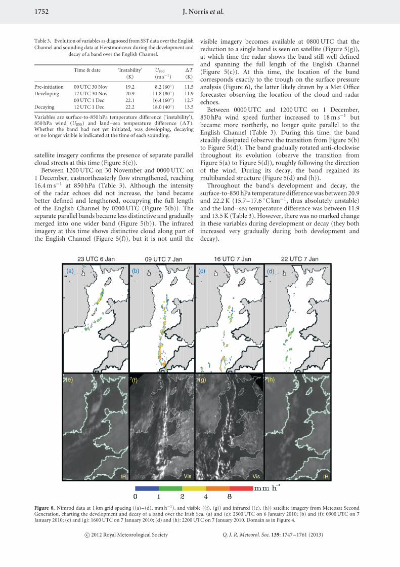
Figure 8. Nimrod data at 1 km grid spacing ((a)–(d), mm h−1), and visible ((f), (g)) and infrared ((e), (h)) satellite imagery from Meteosat SecondGeneration, charting the development and decay of a band over the Irish Sea. (a) and (e): 2300 UTC on 6 January 2010; (b) and (f): 0900 UTC on 7January 2010; (c) and (g): 1600 UTC on 7 January 2010; (d) and (h): 2200 UTC on 7 January 2010. Domain as in Figure 4.



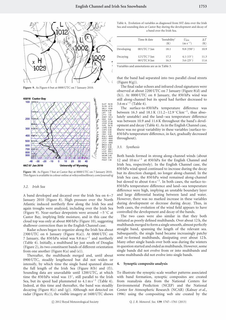
Figure 9. As Figure 6 but at 0000 UTC on 7 January 2010.

Figure 10. As Figure 7 but at Castor Bay at 0000 UTC on 7 January 2010.This figure is available in colour online at wileyonlinelibrary.com/journal/qj

3.2. Irish Sea

A band developed and decayed over the Irish Sea on 6–7January 2010 (Figure 8). High pressure over the NorthAtlantic induced northerly flow along the Irish Sea andagain troughs were analyzed, including over the Irish Sea(Figure 9). Near-surface dewpoints were around −5 ◦C atCastor Bay, implying little moisture, and in this case thecloud top was only at about 800 hPa (Figure 10), suggestingshallower convection than in the English Channel case.

Radar echoes began to organize along the Irish Sea about2300 UTC on 6 January (Figure 8(a)). At 0000 UTC on7 January, the 850 hPa wind was 9.8 m s−1 and northerly(Table 4). Initially, a multiband lay just south of Douglas(Figure 2), its two constituent bands of different orientationfrom one another (Figure 8(a) and (e)).

Thereafter, the multibands merged and, until about0900 UTC, steadily lengthened but did not widen orintensify, by which time the single band spanned almostthe full length of the Irish Sea (Figure 8(b) and (f)).Sounding data are unavailable until 1200 UTC, at whichtime the 850 hPa wind was 15◦, still parallel to the IrishSea, but its speed had plummeted to 4.1 m s−1 (Table 4).Indeed, at this time and thereafter, the band was steadilydecaying (Figure 8(c) and (g)). Although not detected onradar (Figure 8(c)), the visible imagery at 1600 UTC shows

Table 4. Evolution of variables as diagnosed from SST data over the IrishSea and sounding data at Castor Bay during the development and decay of

a band over the Irish Sea.

Time & date ‘Instability’ U850 �T(K) (m s−1) (K)

Developing 00 UTC 7 Jan 18.1 9.8 (350◦) 10.9

Decaying 12 UTC 7 Jan 17.2 4.1 (15◦) 11.300 UTC 8 Jan 16.3 3.6 (25◦) 11.6

Variables and annotations are as in Table 3.

that the band had separated into two parallel cloud streets(Figure 8(g)).

The final radar echoes and infrared cloud signatures wereobserved at about 2200 UTC on 7 January (Figure 8(d) and(h)). At 0000 UTC on 8 January, the 850 hPa wind wasstill along-channel but its speed had further decreased to3.6 m s−1 (Table 4).

The surface-to-850 hPa temperature difference wasbetween 16.3 and 18.1 K (11.2–12.9 ◦C km−1, thus abso-lutely unstable) and the land–sea temperature differencewas between 10.9 and 11.6 K throughout the band’s devel-opment and decay (Table 4). As in the English Channel case,there was no great variability in these variables (surface-to-850 hPa temperature difference, in fact, gradually decreasedthroughout).

3.3. Synthesis

Both bands formed in strong along-channel winds (about12 and 10 m s−1 at 850 hPa for the English Channel andIrish Sea, respectively). In the English Channel case, the850 hPa wind speed continued to increase during the decaybut its direction changed, no longer along-channel. In theIrish Sea case, the 850 hPa wind remained along-channelbut slowed to about 4 m s−1. In both cases, the surface-to-850 hPa temperature difference and land–sea temperaturedifference were high, implying an unstable boundary layerand large differential heating between land and water.However, there was no marked increase in these variablesduring development or decrease during decay. Thus, inboth cases, the evolution of the wind field appears to havecontrolled the development and decay of the bands.

The two cases were also similar in that they bothinitiated as poorly defined multibands. Over about 12 h, themultibands merged to form a single smooth, almost perfectlystraight band, spanning the length of the relevant sea.Subsequently, the single band became increasingly patchyand re-formed multibands, dissipating over about 12 h.Many other single bands over both seas during the wintersin question started and ended as multibands. However, somesingle bands did not evolve from or into multibands andsome multibands did not evolve into single bands.

4. Synoptic composite analysis

To illustrate the synoptic-scale weather patterns associatedwith band formation, synoptic composites are createdfrom reanalysis data from the National Centers forEnvironmental Prediction (NCEP) and the NationalCenter for Atmospheric Research (NCAR) (Kalnay et al.,1996) using the compositing web site created by the



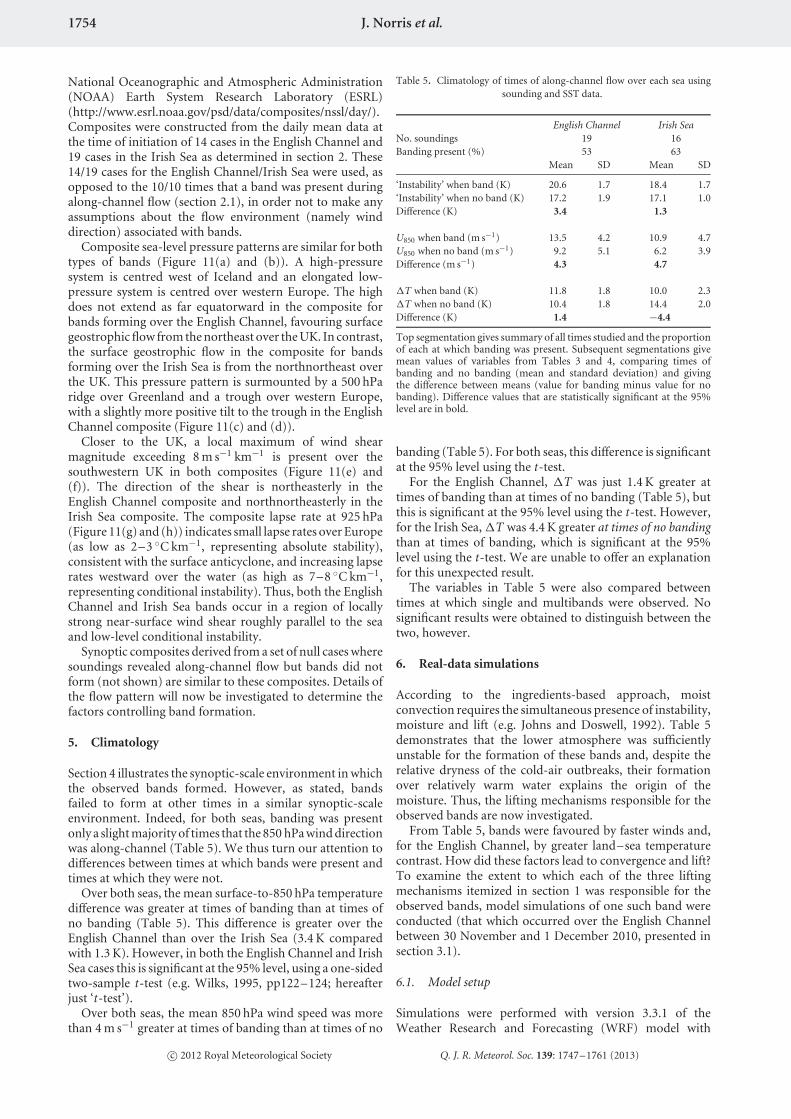
National Oceanographic and Atmospheric Administration(NOAA) Earth System Research Laboratory (ESRL)(http://www.esrl.noaa.gov/psd/data/composites/nssl/day/).Composites were constructed from the daily mean data atthe time of initiation of 14 cases in the English Channel and19 cases in the Irish Sea as determined in section 2. These14/19 cases for the English Channel/Irish Sea were used, asopposed to the 10/10 times that a band was present duringalong-channel flow (section 2.1), in order not to make anyassumptions about the flow environment (namely winddirection) associated with bands.

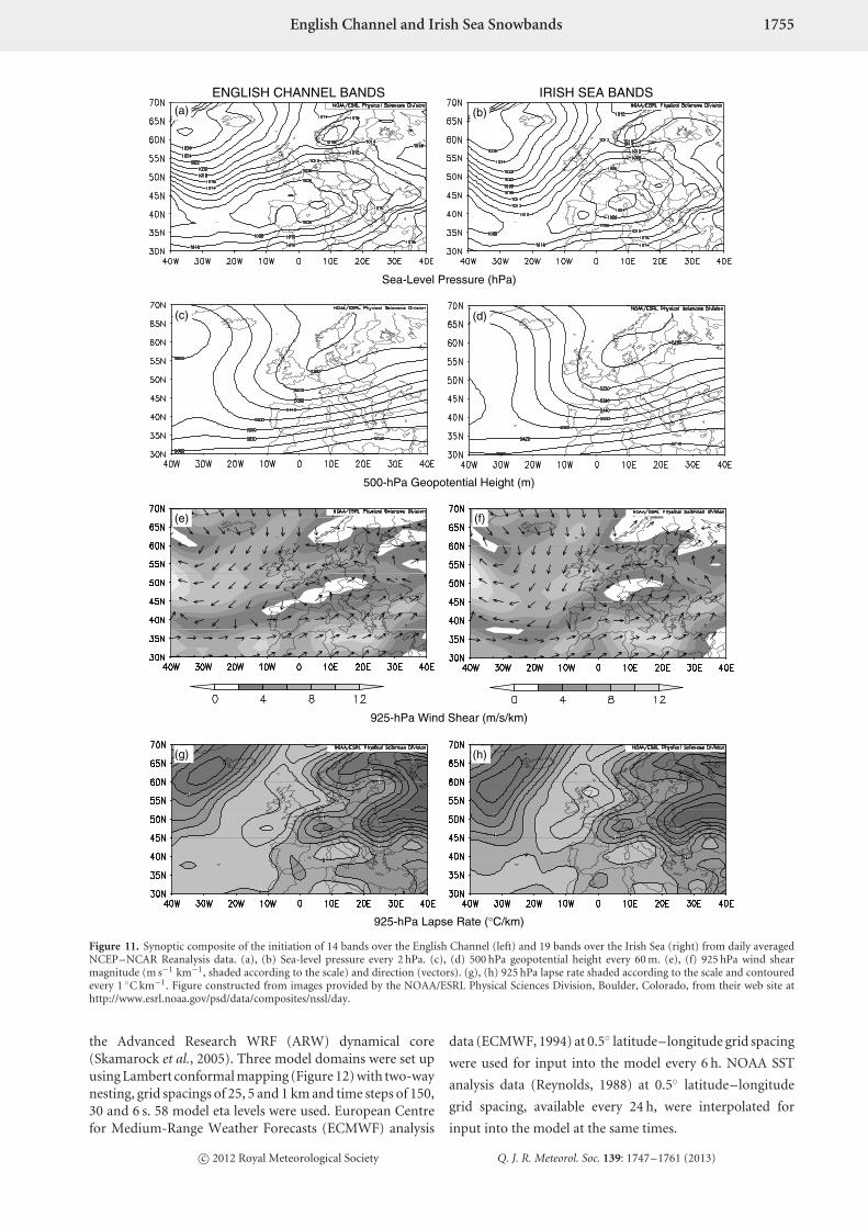
Composite sea-level pressure patterns are similar for bothtypes of bands (Figure 11(a) and (b)). A high-pressuresystem is centred west of Iceland and an elongated low-pressure system is centred over western Europe. The highdoes not extend as far equatorward in the composite forbands forming over the English Channel, favouring surfacegeostrophic flow from the northeast over the UK. In contrast,the surface geostrophic flow in the composite for bandsforming over the Irish Sea is from the northnortheast overthe UK. This pressure pattern is surmounted by a 500 hParidge over Greenland and a trough over western Europe,with a slightly more positive tilt to the trough in the EnglishChannel composite (Figure 11(c) and (d)).

Closer to the UK, a local maximum of wind shearmagnitude exceeding 8 m s−1 km−1 is present over thesouthwestern UK in both composites (Figure 11(e) and(f)). The direction of the shear is northeasterly in theEnglish Channel composite and northnortheasterly in theIrish Sea composite. The composite lapse rate at 925 hPa(Figure 11(g) and (h)) indicates small lapse rates over Europe(as low as 2–3 ◦C km−1, representing absolute stability),consistent with the surface anticyclone, and increasing lapserates westward over the water (as high as 7–8 ◦C km−1,representing conditional instability). Thus, both the EnglishChannel and Irish Sea bands occur in a region of locallystrong near-surface wind shear roughly parallel to the seaand low-level conditional instability.

Synoptic composites derived from a set of null cases wheresoundings revealed along-channel flow but bands did notform (not shown) are similar to these composites. Details ofthe flow pattern will now be investigated to determine thefactors controlling band formation.

5. Climatology

Section 4 illustrates the synoptic-scale environment in whichthe observed bands formed. However, as stated, bandsfailed to form at other times in a similar synoptic-scaleenvironment. Indeed, for both seas, banding was presentonly a slight majority of times that the 850 hPa wind directionwas along-channel (Table 5). We thus turn our attention todifferences between times at which bands were present andtimes at which they were not.

Over both seas, the mean surface-to-850 hPa temperaturedifference was greater at times of banding than at times ofno banding (Table 5). This difference is greater over theEnglish Channel than over the Irish Sea (3.4 K comparedwith 1.3 K). However, in both the English Channel and IrishSea cases this is significant at the 95% level, using a one-sidedtwo-sample t-test (e.g. Wilks, 1995, pp122–124; hereafterjust ‘t-test’).

Over both seas, the mean 850 hPa wind speed was morethan 4 m s−1 greater at times of banding than at times of no

Table 5. Climatology of times of along-channel flow over each sea usingsounding and SST data.

English Channel Irish SeaNo. soundings 19 16Banding present (%) 53 63

Mean SD Mean SD

‘Instability’ when band (K) 20.6 1.7 18.4 1.7‘Instability’ when no band (K) 17.2 1.9 17.1 1.0Difference (K) 3.4 1.3

U850 when band (m s−1) 13.5 4.2 10.9 4.7U850 when no band (m s−1) 9.2 5.1 6.2 3.9Difference (m s−1) 4.3 4.7

�T when band (K) 11.8 1.8 10.0 2.3�T when no band (K) 10.4 1.8 14.4 2.0Difference (K) 1.4 −4.4

Top segmentation gives summary of all times studied and the proportionof each at which banding was present. Subsequent segmentations givemean values of variables from Tables 3 and 4, comparing times ofbanding and no banding (mean and standard deviation) and givingthe difference between means (value for banding minus value for nobanding). Difference values that are statistically significant at the 95%level are in bold.

banding (Table 5). For both seas, this difference is significantat the 95% level using the t-test.

For the English Channel, �T was just 1.4 K greater attimes of banding than at times of no banding (Table 5), butthis is significant at the 95% level using the t-test. However,for the Irish Sea, �T was 4.4 K greater at times of no bandingthan at times of banding, which is significant at the 95%level using the t-test. We are unable to offer an explanationfor this unexpected result.

The variables in Table 5 were also compared betweentimes at which single and multibands were observed. Nosignificant results were obtained to distinguish between thetwo, however.

6. Real-data simulations

According to the ingredients-based approach, moistconvection requires the simultaneous presence of instability,moisture and lift (e.g. Johns and Doswell, 1992). Table 5demonstrates that the lower atmosphere was sufficientlyunstable for the formation of these bands and, despite therelative dryness of the cold-air outbreaks, their formationover relatively warm water explains the origin of themoisture. Thus, the lifting mechanisms responsible for theobserved bands are now investigated.

From Table 5, bands were favoured by faster winds and,for the English Channel, by greater land–sea temperaturecontrast. How did these factors lead to convergence and lift?To examine the extent to which each of the three liftingmechanisms itemized in section 1 was responsible for theobserved bands, model simulations of one such band wereconducted (that which occurred over the English Channelbetween 30 November and 1 December 2010, presented insection 3.1).

6.1. Model setup

Simulations were performed with version 3.3.1 of theWeather Research and Forecasting (WRF) model with



ENGLISH CHANNEL BANDS IRISH SEA BANDS(a)

(f)(e)

(d)(c)

(b)

Sea-Level Pressure (hPa)

925-hPa Wind Shear (m/s/km)

500-hPa Geopotential Height (m)

(h)(g)

925-hPa Lapse Rate (°C/km)

Figure 11. Synoptic composite of the initiation of 14 bands over the English Channel (left) and 19 bands over the Irish Sea (right) from daily averagedNCEP–NCAR Reanalysis data. (a), (b) Sea-level pressure every 2 hPa. (c), (d) 500 hPa geopotential height every 60 m. (e), (f) 925 hPa wind shearmagnitude (m s−1 km−1, shaded according to the scale) and direction (vectors). (g), (h) 925 hPa lapse rate shaded according to the scale and contouredevery 1 ◦C km−1. Figure constructed from images provided by the NOAA/ESRL Physical Sciences Division, Boulder, Colorado, from their web site athttp://www.esrl.noaa.gov/psd/data/composites/nssl/day.

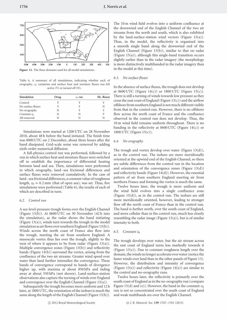
the Advanced Research WRF (ARW) dynamical core(Skamarock et al., 2005). Three model domains were set upusing Lambert conformal mapping (Figure 12) with two-waynesting, grid spacings of 25, 5 and 1 km and time steps of 150,30 and 6 s. 58 model eta levels were used. European Centrefor Medium-Range Weather Forecasts (ECMWF) analysis

data (ECMWF, 1994) at 0.5◦ latitude–longitude grid spacing

were used for input into the model every 6 h. NOAA SST

analysis data (Reynolds, 1988) at 0.5◦ latitude–longitude

grid spacing, available every 24 h, were interpolated for

input into the model at the same times.



Figure 12. The three domains used for all model simulations.

Table 6. A summary of all simulations, indicating whether each oforography, z0 variations and surface heat and moisture fluxes was left

active (Y) or turned off (N).

Simulation Orog. z0 var. Sfc. fluxes

Control Y Y YNo surface fluxes Y Y NNo orography N Y YConstant z0 N N YAll removed N N N

Simulations were started at 1200 UTC on 28 November2010, about 48 h before the band initiated. The finish timewas 0000 UTC on 2 December, about three hours after theband dissipated. Grid-scale noise was removed by addingsixth-order numerical diffusion.

A full-physics control run was performed, followed by arun in which surface heat and moisture fluxes were switchedoff to establish the importance of differential heatingbetween land and sea. Then, simulations were performedin which orography, land–sea frictional differences andsurface fluxes were removed cumulatively. In the case ofland–sea frictional differences, a constant value of roughnesslength, z0 = 0.2 mm (that of open sea), was set. Thus, fivesimulations were performed (Table 6), the results of each ofwhich are described in turn.

6.2. Control run

A sea-level-pressure trough forms over the English Channel(Figure 13(b)). At 0600 UTC on 30 November (42 h intothe simulation), as the radar shows the band initiating(Figure 13(a)), winds turn towards the trough in the modelsimulation as air flows over southern England (Figure 13(b)).Winds across the north coast of France also flow intothe trough, meeting the air from southern England. Amesoscale vortex thus lies over the trough, slightly to thewest of where it appears to be from radar (Figure 13(a)).Multiple convergence zones (Figure 13(b)) and reflectivitybands (Figure 14(b)) surround the vortex, arising from theconfluence of the two air streams. Greater wind speed overwater than land further intensifies the convergence. Thesebands of convergence correspond to bands of divergencehigher up, with maxima at about 850 hPa and fadingaway at about 550 hPa (not shown). Land-surface-stationobservations also capture the turning of winds over Englandand convergence over the English Channel (Figure 13(a)).

Subsequently the trough becomes more uniform and 12 hlater, at 1800 UTC, the orientation of the isobars is much thesame along the length of the English Channel (Figure 15(b)).

The 10 m wind field evolves into a uniform confluence atthe downwind end of the English Channel of the two airstreams from the north and south, which is also exhibitedby the land-surface-station wind vectors (Figure 15(a)).Thus, in the model, the reflectivity is organized intoa smooth single band along the downwind end of theEnglish Channel (Figure 15(b)), similar to that on radar(Figure 15(a)), although this single-band transition occursslightly earlier than in the radar imagery (the morphologyis more distinctively multibanded in the radar imagery thanin the model at this time).

6.3. No surface fluxes

In the absence of surface fluxes, the trough does not developat 0600 UTC (Figure 14(c)) or 1800 UTC (Figure 15(c)).There is still a turning of winds towards low pressure as theycross the east coast of England (Figure 13(c)) and the airflowoffshore from southern England is not much different visiblyfrom that in the control run. However, there is no offshoreflow across the north coast of France and the confluenceobserved in the control run does not develop. Thus, the10 m wind field remains uniform throughout. There is nobanding in the reflectivity at 0600 UTC (Figure 14(c)) or1800 UTC (Figure 15(c)).

6.4. No orography

The trough and vortex develop over water (Figure 13(d)),as in the control run. The isobars are more meridionallyoriented at the upwind end of the English Channel, so thereare subtle differences from the control run in the locationand orientation of the convergence zones (Figure 13(d))and reflectivity bands (Figure 14(d)). However, the essentialpattern of air from southern England meeting air fromnorthern France and forming the vortex is much the same.

Twelve hours later, the trough is more uniform andthe wind field evolves into a single confluence zone(Figure 15(d)), as in the control run. The isobars are stillmore meridionally oriented, however, leading to strongerflow off the north coast of France than in the control run.The band is further north, over the south coast of England,and more cellular than in the control run, much less closelyresembling the radar image (Figure 15(a)), but is of similarintensity to both.

6.5. Constant z0

The trough develops over water, but the air stream acrossthe east coast of England turns less markedly towards it(Figure 13(e)). Due to constant roughness length over thedomain, the winds no longer accelerate over water (notice thefaster winds over land than in the other panels of Figure 13).However, the distribution and intensity of convergence(Figure 13(e)) and reflectivity (Figure 14(e)) are similar tothe control and no-orography runs.

Twelve hours later, the reflectivity is primarily over thesouth coast of England as in the no-orography run (compareFigure 15(d) and (e)). However, the band in the constant-z0

run is not so concentrated over the south coast of Englandand weak multibands are over the English Channel.



Figure 13. Observations (a) and model output (b–f) at 0600 UTC on 30 November (42 h into the simulation). (a) shows Nimrod precipitation rate(mm h−1) and wind vectors taken from Met Office Integrated Data Archive System (MIDAS) land surface stations (m s−1). (b)–(f) show sea-levelpressure (grey contours every 1 hPa, high pressure to the north), 10 m wind divergence (m s−1 km−1, negative values shaded), and 10 m wind vectors(m s−1). (b) Control run; (c) no surface fluxes; (d) no orography; (e) no orography and constant z0; (f) all removed. Domain as in Figure 3.

6.6. All removed

As in section 6.3, the removal of surface fluxes preventsconvergence (Figure 13(f)) and organized precipitation(Figures 14(f) and 15(f)) from forming. The main differencebetween this run and the no-surface-fluxes run (in whichorography and frictional variations remained) is that thereis no turning of the winds towards low pressure to thesouth as they cross the east coast of England. However,this is immaterial because, as demonstrated by the no-surface-fluxes run, this effect alone is insufficient to generateconvergence over the English Channel.

6.7. Later initialization times

The same simulations were performed with various otherinitialization times (not shown). In control runs initializedlater, the location and morphology of the band in itsorganized stage much more closely resembled the radar

imagery than in Figure 15(b). However, the correspondingsensitivity experiments differed little from the controlrun, due to insufficient spin-up time. Thus, because thepurpose of this article is to investigate the physics ofthe snowbands rather than to produce the most accuratesimulation possible, we have presented the simulations withsufficient spin-up time for each sensitivity simulation toevolve distinctly. We maintain that the larger differencesbetween the observed and modelled bands with the earlierinitialization time do not change the conclusions that can bedrawn from these simulations. Instead, we have attemptedto provide an overview of the identified physical processes(orography, z0 variations, surface fluxes) involved in bandformation.

6.8. Irish Sea

The band documented over the Irish Sea in section 3.2 wasalso simulated with the same domains (but without the



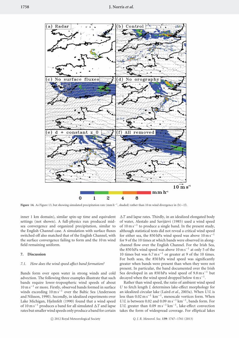
Figure 14. As Figure 13, but showing simulated precipitation rate (mm h−1, shaded) rather than 10 m wind divergence in (b)–(f).

inner 1 km domain), similar spin-up time and equivalentsettings (not shown). A full-physics run produced mid-sea convergence and organized precipitation, similar tothe English Channel case. A simulation with surface fluxesswitched off also matched that of the English Channel, withthe surface convergence failing to form and the 10 m windfield remaining uniform.

7. Discussion

7.1. How does the wind speed affect band formation?

Bands form over open water in strong winds and coldadvection. The following three examples illustrate that suchbands require lower-tropospheric wind speeds of about10 m s−1 or more. Firstly, observed bands formed in surfacewinds exceeding 10 m s−1 over the Baltic Sea (Anderssonand Nilsson, 1990). Secondly, in idealized experiments overLake Michigan, Hjelmfelt (1990) found that a wind speedof 10 m s−1 produces a band for all simulated �T and lapserates but smaller wind speeds only produce a band for certain

�T and lapse rates. Thirdly, in an idealized elongated bodyof water, Alestalo and Savijarvi (1985) used a wind speedof 10 m s−1 to produce a single band. In the present study,although statistical tests did not reveal a critical wind speedfor either sea, the 850 hPa wind speed was above 10 m s−1

for 9 of the 10 times at which bands were observed in along-channel flow over the English Channel. For the Irish Sea,the 850 hPa wind speed was above 10 m s−1 at only 5 of the10 times but was 6.7 m s−1 or greater at 9 of the 10 times.For both seas, the 850 hPa wind speed was significantlygreater when bands were present than when they were notpresent. In particular, the band documented over the IrishSea developed in an 850 hPa wind speed of 9.8 m s−1 butdecayed when the wind speed dropped below 4 m s−1.

Rather than wind speed, the ratio of ambient wind speedU to fetch length L determines lake-effect morphology foran idealized circular lake (Laird et al., 2003a). When U/L isless than 0.02 m s−1 km−1, mesoscale vortices form. WhenU/L is between 0.02 and 0.09 m s−1 km−1, bands form. ForU/L greater than 0.09 m s−1 km−1, lake-effect convectiontakes the form of widespread coverage. For elliptical lakes



Figure 15. As Figure 14 but at 1800 UTC (54 h into the simulation).

with an aspect ratio of 9:1 (roughly that of the EnglishChannel and Irish Sea) and flow parallel to the long axis, thethreshold for bands is lowered to 0.017 (Laird et al., 2003b).Given that the English Channel and Irish Sea are bothroughly 500 km long, U/L = 0.09 corresponds to 45 m s−1.This value is rarely exceeded at low levels over the UK andindeed widespread coverage has not been documented overthe English Channel and Irish Sea. However, U/L = 0.017corresponds to 8.5 m s−1. Thus, there is a rough consistencybetween the observational results in this study and thecriteria in the Laird et al. studies. Additional observationaland modelling studies could further refine these criteria forthe waters around the UK.

7.2. How does the lower boundary condition affect bandformation?

Previous studies of similar bands have discussed therelative importance of orography and land–sea frictionaldifferences. For example, Andersson and Gustafsson (1994)found that coastal orography was of secondary importanceto forming snowbands over the Baltic Sea, and Onton

and Steenburgh (2001) found that the orography was notresponsible for band formation over the Great Salt Lakebut merely altered the distribution of the snowfall. In oursimulations of the snowband over the English Channel, theremoval of orography resulted in the band being composedof more cellular convection but did not alter its existence.

Even without the orography, some authors have foundland–sea frictional differences to be of primary importancein forming convergence for quasi-stationary bands overwater. For example, using an idealized hydrostatic model,Alestalo and Savijarvi (1985) found that a geostrophic windof 10 m s−1 along the major axis of an elongated body ofwater was sufficient to induce convergence due to frictionaldifference alone, even when the land and sea are the sametemperature and the atmosphere is neutrally stratified.Roeloffzen et al. (1986) also found frictional convergencealone to be sufficient to produce a quasi-stationary cloudband parallel to an idealized coastline. In our simulations,setting the roughness length z0 as a constant caused windscrossing the east coast of England to turn less towards thetrough over the English Channel than in the control run.The constant-z0 run also produced multibands at a later



time, with a less well-defined reflectivity maximum than inthe control and no-orography runs. Thus, our simulationsshow that frictional differences enhance band intensity buttheir absence does not preclude band formation.

7.3. Are the bands caused by land breezes?

Given that the classic land breeze is a circulation resultingfrom the diurnal variation in heating under relativelybenign synoptic situations, particularly during the warmseason, we question its applicability to these snowbands.Our interpretation is based upon the following evidence.

(1) No diurnal cycle in the initiation of the observedsnowbands was evident.

(2) The land–sea temperature difference changed littleduring the band’s development and decay (thetemperature difference gradually increased; seeTable 3), implying that the band was not diurnallydriven.

Some authors have interpreted the land-breeze concept morebroadly as a thermally driven offshore flow superimposedon an along-shore ambient wind, free from any diurnalinfluence, and have attributed along-shore snowbands tothe collision of these land breezes from opposing shores (e.g.Passarelli and Braham, 1981; Savijarvi, 2012). In accordancewith this relaxed definition, the American MeteorologicalSociety (AMS) Glossary states that the land breeze ‘usually’blows at night (http://amsglossary.allenpress.com/glossary).In our simulation of the band over the English Channel,there was indeed strong offshore flow across the north coastof France that failed to develop in the absence of surfacefluxes and was essentially the same in the no-orography andconstant-z0 runs. Thus, this aspect to the flow was largelythermally driven and qualifies as a land breeze as defined bythe above authors and in the AMS Glossary. However, therewas no major difference in the flow from southern Englandin the control run and no-surface-fluxes run.

This asymmetry between the two coasts may be explainedby Atlas et al. (1983). They found that, during cold-airoutbreaks, a bay that is concave in the downwind directionleads to offshore convergence downwind because the part ofthe air stream that has had a shorter trajectory over the warmwater experiences less heating than the other trajectories.Thus, there is differential heating and the higher pressureair that has travelled less distance over water flows towardsthe lower pressure air further offshore. For this case, thenorth coast of France is divided into two such bays that areconcave facing downwind (east and west of the CherbourgPeninsula, Figure 2) and along each of these there is strongturning of the winds towards the air that has travelledfurther over water (to the right). This was also observedover the English Channel in the modelling experiments ofMonk (1987). The south coast of England, on the otherhand, is almost a straight line, which does not allow for thiseffect.

Combining the evidence from sections 7.1, 7.2 and 7.3,the snowband is the mesoscale response to surface heatingof cold-air advection over warm water, as first describedby Lavoie (1972). The roles of orography and frictionaldifferences may affect the timing or location of the band butdo not fundamentally alter its occurrence.

8. Conclusions

Quasi-stationary wind-parallel snowbands formed along themajor axis of the English Channel and Irish Sea during cold-air outbreaks in the winters of 2009–10 and 2010–11. Thesebands bear similarity to those in other parts of the world:Great Lakes, Great Salt Lake, New England, off the northcoast of Germany, Sea of Japan and the Baltic Sea. Theywere studied using the analysis of observational data (e.g.radar imagery, satellite imagery, surface and upper-air data),synoptic composites, climatology and real-data numericalmodelling. Two different morphologies of bands wereidentified: single bands and multibands. Unfortunately, theclimatology in section 5 was unable to identify distinguishingcharacteristics between these two morphologies, suggestingthat the environmental factors tested in this study (e.g.wind direction, land–sea temperature difference) werenot responsible for the single or multiband morphology.However, case studies over both seas in section 3 indicatedthat multibands occurred during the formation and decaystages of mature single-band cases, which was commonly(although not always) observed during the winters inquestion.

The case studies showed that bands formed over theEnglish Channel and Irish Sea when winds were greater thanabout 10 m s−1 and nearly parallel to the long axis of thewater body. The surface-to-850 hPa temperature differenceexceeded 18 K and the land–sea temperature differenceexceeded 10 K. The band over the English Channel decayedwhen the wind direction was no longer along-channel. Theband over the Irish Sea decayed when the wind speeddecreased markedly.

Synoptic composites showed that bands formed with aridge over Greenland and a trough over western Europe at500 hPa. A surface anticyclone was centred west of Icelandand a zonally elongated cyclone was centred over westernEurope. Synoptic composites were similar, however, fortimes at which bands were not present, demonstratingthat band occurrence depends on the finer details of theflow environment. In support of this, surface-to-850 hPatemperature difference and 850 hPa wind speed were bothfound to be significantly greater at times of banding thanfor no banding. Thus the observed bands formed whenconvection resulted from pronounced instability over water,with that convection organized into bands for sufficientlystrong winds.

Model sensitivity experiments were performed for onesuch band over the English Channel. In the control run, atrough in sea-level pressure formed over the English Channeland surface winds turned cyclonically towards the trough asthey passed from the North Sea over the east of England.Over the English Channel, these winds met an air streamoffshore from northern France, forming a mesoscale vortexand strong convergence zones over the English Channel.Precipitation bands formed over the convergence lines. Overthe course of about 12 h, the trough intensified, forminga single convergence line and precipitation band at thedownwind end.

Removing the orography and setting the roughness lengthconstant across land and sea produced a weaker trough anddifferences in the timing, location and intensity of theband, but the band was still present, despite less turningof the winds over southern England towards the trough.The removal of surface heat and moisture fluxes, both with



and without orography and z0 variations, resulted in thecomplete failure of convergence and organized precipitationto develop. We therefore conclude that these fluxes are themajor factor in generating the observed snowbands.

Acknowledgements

The Nimrod data used in this study were provided bythe Met Office through the British Atmospheric DataCentre (BADC). ECMWF analyses were obtained usingthe ECMWF Meteorological Archive and Retrieval System(MARS) software. Sounding data were provided mainlyby the Department of Atmospheric Science, University ofWyoming, but some were only available through BADC.Meteosat images and MIDAS land-surface-station data werealso accessed through BADC. We thank Karen Barfoot of theMet Office for providing SST data, NOAA/ESRL PhysicalSciences Division for construction of the composites inFigure 11 from their web page and Bogdan Antonescu andHugo Ricketts for use of their script to process the rawNimrod data. We also thank the anonymous reviewers andKeith Browning, who all provided helpful comments on theinitial version of the manuscript. Jesse Norris is a NERC-funded student through the DIAMET (DIAbatic influenceson Mesoscale structures in ExTratropical storms) project,NE/I005234/1.

References

Alestalo M, Savijarvi H. 1987. Mesoscale circulations in a hydrostaticmodel: Coastal convergence and orographic lifting. Tellus 37A:156–162.

Andersson T, Gustafsson N. 1994. Coast of departure and coast ofarrival: Two important concepts for the formation and structure ofconvective snowbands over seas and lakes. Mon. Weather Rev. 122:1036–1049.

Andersson T, Nilsson S. 1990. Topographically induced convectivesnowbands over the Baltic Sea and their precipitation distribution.Weather and Forecasting 5: 299–312.

Asai T. 1970. Stability of a plane parallel flow with variable vertical shearand unstable stratification. J. Meteorol. Soc. Jpn 48: 129–139.

Atlas D, Chou SH, Byerly WP. 1983. The influence of coastal shapeon winter mesoscale air–sea interaction. Mon. Weather Rev. 111:245–252.

Bader MJ, Forbes GS, Grant JR, Lilley RBE. 1995. Images in WeatherForecasting: A Practical Guide for Interpreting Satellite and RadarImagery. Cambridge University Press: Cambridge, UK; 499pp.

Benard H. 1900. Les tourbillons cellulaires dans une nappe liquid. Rev.Gen. Sci. Pures Appl. II: 1261–1271, 1309–1328.

Bosart LF. 1975. New England coastal frontogenesis. Q. J. R. Meteorol.Soc. 101: 957–978.

Braham RR Jr. 1983. The Midwest snowstorm of 8–11 December 1977.Mon. Weather Rev. 111: 253–272.

Browning KB, Ecclestone AJ, Monk GA. 1985. The use of satellite andradar imagery to identify persistent shower bands downwind of theNorth Channel. Meteorol. Mag. 114: 325–331.

European Centre for Medium-range Weather Forecasts (ECMWF). 1994.‘Description of the ECMWF/WCRP Level III-A Global AtmosphericData Archive’. ECMWF: Reading, UK.

Guernsey Meteorological Office. 2011. ‘Guernsey Airport MeteorologicalOffice – Annual Report 2010’. States of Guernsey Public ServicesDepartment: Guernsey, Channel Islands.

Harrison DL, Scovell RW, Kitchen M. 2009. High-resolutionprecipitation estimates for hydrological uses. Proceedings of theInstitution of Civil Engineers – Water Management 162: 125–135.

Hjelmfelt MR. 1990. Numerical study of the influence of environmentalconditions on lake-effect snowstorms over Lake Michigan. Weatherand Forecasting 118: 138–150.

Johns RH, Doswell CA III. 1992. Severe local storms forecasting. Mon.Weather Rev. 7: 588–612.

Kalnay E, Kanamitsu M, Kistler R, Collins W, Deaven D, Gandin L,Iredell M, Saha S, White G, Woollen J, Zhu Y, Chelliah M,Ebisuzaki W, Higgins W, Janowiak J, Mo KC, Ropelewski C, Wang J,Leetmaa A, Reynolds R, Jenne R, Joseph D. 1996. The NCEP/NCAR40-year Reanalysis project. Bull. Am. Meteorol. Soc. 77: 437–471.

Kuo HL. 1963. Perturbations of plane Couette flow in stratified fluidand origin of cloud streets. Phys. Fluids 6: 195–211.

Laird NF, Kristovich DAR, Walsh JE. 2003a. Idealized model simulationsexamining the mesoscale structure of winter lake-effect circulations.Mon. Weather Rev. 131: 206–221.

Laird NF, Walsh JE, Kristovich DAR. 2003b. Model simulationsexamining the relationship of lake-effect morphology to lake shape,wind direction, and wind speed. Mon. Weather Rev. 131: 2102–2111.

Lavoie RL. 1972. A mesoscale numerical model of lake-effect storms.J. Atmos. Sci. 29: 1025–1040.

Miura Y. 1986. Aspect ratios of longitudinal rolls and convection cellsobserved during cold air outbreaks. J. Atmos. Sci. 43: 26–39.

Monk GA. 1987. ‘Topographically related convection over the BritishIsles’. In Satellite and Radar Imagery Interpretation: Preprints for aworkshop held at Meteorological Office College, Shinfield Park, Reading,20-24 July, 1987; 305–324. Meteorological Office: Exeter, UK.

Monk GA, Rowley LHG, Smith F, Bader MJ. 1990.. ‘Climatologiesof topographically related convection over the British Isles’. InProceedings 8th Meteosat Scientific Users Meeting, Norrkoping, Sweden,28–31 August 1990; 121–125. Meteorological Office: Exeter, UK.

Nagata WS. 1987. On the structure of a convergent cloud band over theJapan Sea in winter: A prediction experiment. J. Meteorol. Soc. Jpn 65:871–883.

Niziol TA, Snyder WR, Waldstreicher JS. 1995. Winter weatherforecasting throughout the eastern United States. Part IV: Lake-effectsnow. Weather and Forecasting 10: 61–77.

Onton DJ, Steenburgh WJ. 2001. Diagnostic and sensitivity studies of the7 December 1998 Great Salt Lake-effect snowstorm. Mon. WeatherRev. 129: 1318–1338.

Passarelli RE Jr, Braham RR Jr. 1981. The role of the winter land breezein the formation of Great Lake snowstorms. Bull. Am. Meteorol. Soc.62: 482–491.

Peace RL Jr, Sykes RB Jr. 1966. Mesoscale study of a lake-effectsnowstorm. Mon. Weather Rev. 94: 495–507.

Pike WS. 1990. A heavy mesoscale snowfall event in northern Germany.Meteorol. Mag. 119: 187–195.

Rayleigh L. 1916. On convection currents in a horizontal layer of fluidwhen the higher temperature is on the underside. Philos. Mag. 32:529–546.

Reynolds R. 1988. A real-time global sea surface temperature analysis.J. Climate 1: 75–86.

Roeloffzen JC, Van Den Berg WD, Oerlemans J. 1986. Frictionalconvergence at coastlines. Tellus 38A: 397–411.

Savijarvi H. 2012. Cold air outbreaks over high-latitude sea gulfs. Tellus64A: 1–11.

Schultz DM. 1999. Lake-effect snowstorms in northern Utah and westernNew York with and without lightning. Weather and Forecasting 14:1023–1031.

Schultz DM, Vavrek RJ. 2010. An overview of thundersnow. Weather 64:274–277.

Schultz DM, Arndt DS, Stensrud DJ, Hanna JW. 2004. Snowbandsduring the cold-air outbreak of 23 January 2003. Mon. Weather Rev.132: 827–842.

Shirer HN. 1986. On cloud street development in three dimensions:Parallel and Rayleigh instabilities. Contrib. Atmos. Phys. 59: 126–149.

Skamarock WC, Klemp JB, Dudhia J, Gill DO, Barker DM, Wang W,Powers JG. 2005.. ‘A description of the Advanced Research WRFVersion 2’, NCAR Technical Note NCAR/TN-468+STR; p 88. NCAR:Boulder, CO.

Steenburgh WJ, Onton DJ. 2001. Multiscale analysis of the 7 December1998 Great Salt Lake-effect snowstorm. Mon. Weather Rev. 129:1296–1317.

Steenburgh WJ, Halvorson SF, Onton DJ. 2000. Climatology of lake-effect snow-storms of the Great Salt Lake. Mon. Weather Rev. 128:709–727.

Wilks DS. 1995. Statistical Methods in the Atmospheric Sciences. AcademicPress: New York; 467pp.


Documents

SnowbandsovertheEnglishChannelandIrishSeaduring …weather.seaes.manchester.ac.uk/.../102-Norrisetal13-UKSnowbands.pdf · and organizing around the UK’s coasts (Figure 1). Snow