Embed Size (px)
Citation preview
‘,SMOOTHING FOR TIME-VARYING SYSTEMS USING
MEASUREMENTS CONTAINING COLORED NOISE
Reproduction in whole o r in par t is permitted by the U. S. Government. Distribution of this document is unlimited, -
BY
R . K. Mehra and A . E. Bryson, J r .
Technical Report No. 1
June 1967
Prepared under Grant NGR -22-007-068 2 Divbion of Engineering and Applied Physics
/Harvard University Cambridge, Massachusetts
for
NATIONAL AERONAUTICS AND SPACE ADMINISTRATION
https://ntrs.nasa.gov/search.jsp?R=19670031037 2018-07-08T06:09:13+00:00Z
SMOOTHING FOR LINEAR TIME-VARYING SYSTEMS USING MEASUREMENTS CONTAINING COLORED NOISE
by
R. K. Mehra and A. E. Bryson,Jr .
Division of Engineering and Applied Physics Harvard University Cambridge, Mass.
Abstract
Kalman and Bucy (1961) derived the optimal filter for continuous lin- ea r dynamic systems where - all measurements contain "white noise, I t i.e., noise with correlation times short compared to times of interest in the system. Bryson and Frazier (1962) described the corresponding optimal smoother. (llFilteringtl involves making an estimate at a time t l using measurements made before t 1; "smoothing" involves making an estimate at a time t using measurements made both before and after tl.)
Bryson and Johansen (1965) described the optimal filter for the case 1
where some meas.urements contained either no noise or "colored noise, i. e., noise with correlation times comparable to o r larger than times of interest in the system. The present paper describes the optimal smoother for the case where some measurements contain either no noise o r "colored noise." The problem is formulated as a calculus of varia- tions problem with equality constraints, and is solved using the "sweep method" of McReynolds and Bryson (1965). ment containing colored noise is treated first. and a simple example a r e described.
The case of a single measure- Then the general case
,
1. INTRODUCTION
The Kalman-Bucy fi l ter [ 11 and the Bryson-Frazier smoother [ 21
presume that all measurements contain white noise.
the measurements contain time-correlated noise, or no noise at all, the
correlation matrix of noise in the measurements (usually denoted as R)
is singular. Since the inverse of R appears explicitly in the filtering
and smoothing equations of Refs. [ 11 and [ 23, they cannot be used i f R
is singular.
correlated (or llcoloredll) noise in the measurements can be reduced to a
problem in which some of the measurements contain white noise and others
are perfect.
If some o r all of
By augmenting the state of the system, the problem of time-
The optimal filter for continuous linear dynamic systems using mea-
surements containing time-correlated noise was described by Bryson and
Johansen [3].
on any previous results, and, furthermore, i t leads naturally to the
smoothing results.
Unlike their approach, the present approach does not re ly
To elucidate the method, we shall first consider the case of a single
measurement containing time -correlated nois e.
surement dynamics with system dynamics and augmenting the state of the
system, this case reduces to the case of a system with a scalar perfect
measurement.
After combining mea-
1
2
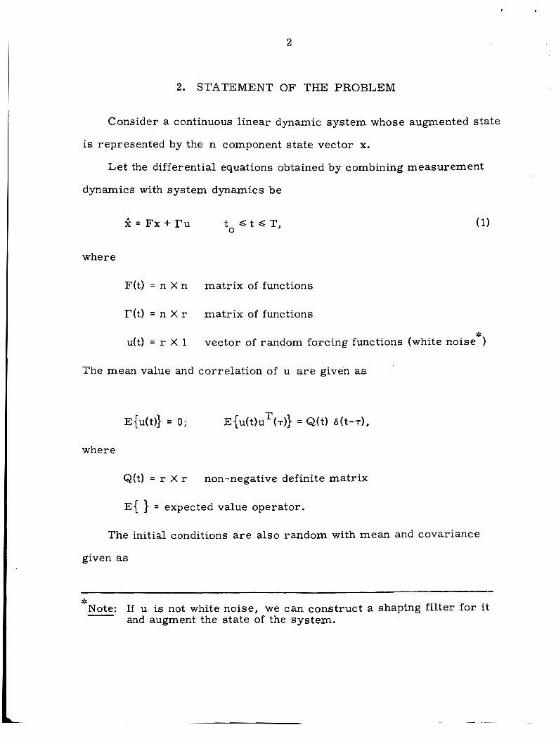
2. STATEMENT OF THE PROBLEM
Consider a continuous linear dynamic system whose augmented state
is represented by the n component s ta te vector x.
Let the differential equations obtained by combining measurement
dynamics with system dynamics be
t s t c r , 0
2 = Fx + Tu
where
F(t) = n X n
r ( t ) = n x r
u(t) = r X 1
matrix of functions
matr ix of functions
vector of random forcing functions (white noise ) *
The mean value and correlation of u a r e given as
E{u(t)} = 0; E{u(t)uT(T)} = Q(t) 6(t-T),
where
Q(t) = r X r non-negative definite matr ix
E{ 1 = expected value operator.
The initial conditions a r e also random with mean and covariance
given as
* Note: If u is not white noise, we can construct a shaping filter for i t
and augment the state of the system.

3
E(x(to)} = 0; E{x(to)x T (to)} = P(to).
It is assumed that u(t) is independent of x(to).
for t ,< t s T. E(x(to)uT(t)} = 0 0
Let z(t) denote the scalar measurement made on the system con-
tinuously from t to T. It is linearly related to the state of the system 0
I
as
t S t t T , T 0
z(t) = h x
where
h(t) = n X 1 vector of functions.
The problem consists in finding the maximum likelihood estimates
of x(t ), x(t), and u(t) for to d t s T using ( d t ) , tostST}. 0
3. FORMULATION O F THE PROBLEM
Since x(t) is a Gauss-Markov random process, the minimum variance
estimate, the maximum likelihood estimate and the min-max estimate a r e
all equal [4]. Hence let us consider the maximum likelihood estimate in
which we t ry to maximize the probability of x and u, given equations of
motion (1) and the set of measurements (2). I
The problem can be stated a s follows. Find x(to) and u(t) to minimize
I Note: F rom here on x and u wi l l denote smoothed estimates of the cor -
responding random variables. This simplifies t;e terminokog . In the l i terature, i t is common to denote these as x(t/T) and u(t7T).
-
4
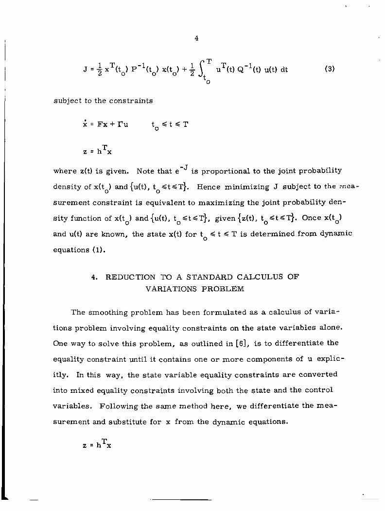
subject to the constraints
i = FX + r u t o G t G T
T z = h x
where z(t) is given.
density of x(to) and {u(t), to Gt a}. surement constraint is equivalent to maximizing the joint probability den-
si ty function of x(to) and{u(t), toCtGT}, given {z(t), to9tCT}. Once x(to)
and u(t) a re known, the state x(t) for to 4 t C T is determined from dynamic
equations ( 1).
Note that e-J is proportional to the joint probability
Hence minimizing J subject to the mea-
4. REDUCTION TO A STANDARD CALCULUS OF VARIATIONS PROBLEM
The smoothing problem has been formulated as a calculus of var ia-
tions problem involving equality constraints on the state variables alone.
One way to solve this problem, as outlined in [SI, is to differentiate the
equality constraint until i t contains one or more components of u explic-
itly.
into mixed equality constraints involving both the s ta te and the control
variables. Following the same method here , we differentiate the mea-
surement and substitute for x f rom the dynamic equations.
In this way, the state variable equality constraints are converted
T z = h x
5
I .
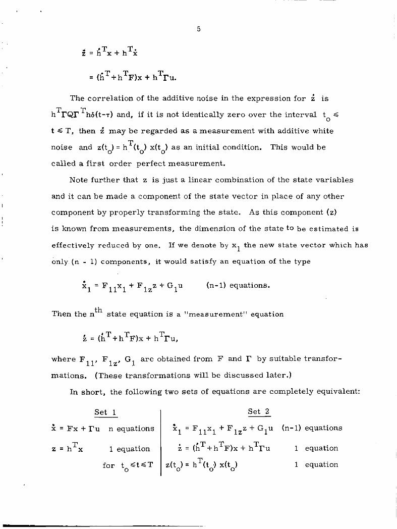
= (hT+hTF)x + h T r u .
The correlation of the additive noise in the expression for k is
h rQr hd(t--r) and, if it is not identically zero over the interval t G
t G T, then 2 may be regarded as a measurement with additive white
noise and z(t ) = h (t ) x(t ) as an initial condition. This would be
called a first order perfect measurement.
T T 0
T 0 0 0
Note further that z is just a linear combination of the state variables
and i t can be made a component of the state vector in place of any other
component by properly transforming the state. A s this component (z)
is known from measurements, the dimension of the state to be estimated is
effectively reduced by one.
only (n - 1) components, it would satisfy an equation of the type
If we denote by x1 the new state vector which has
g1 = F x + F l z z + G 1 u (n- 1) equations. 11 1
Then the nth state equation is a "measurement" equation
' T T T 5 = (h + h F ) x + h r u ,
where FIl , Flz, G1 a r e obtained from F and I' by suitable transfor-
mations. (These transformations wi l l be discussed later.)
In short, the following two sets of equations are completely equivalent:
I Set 1 Set 2
= F x 4- F z + G1u (n-1) equations 11 1 l z S = FX + r u n equations
T z = h x T 1 equation I k = ( i T + h T F ) x + h r u 1 equation
1 equation
6
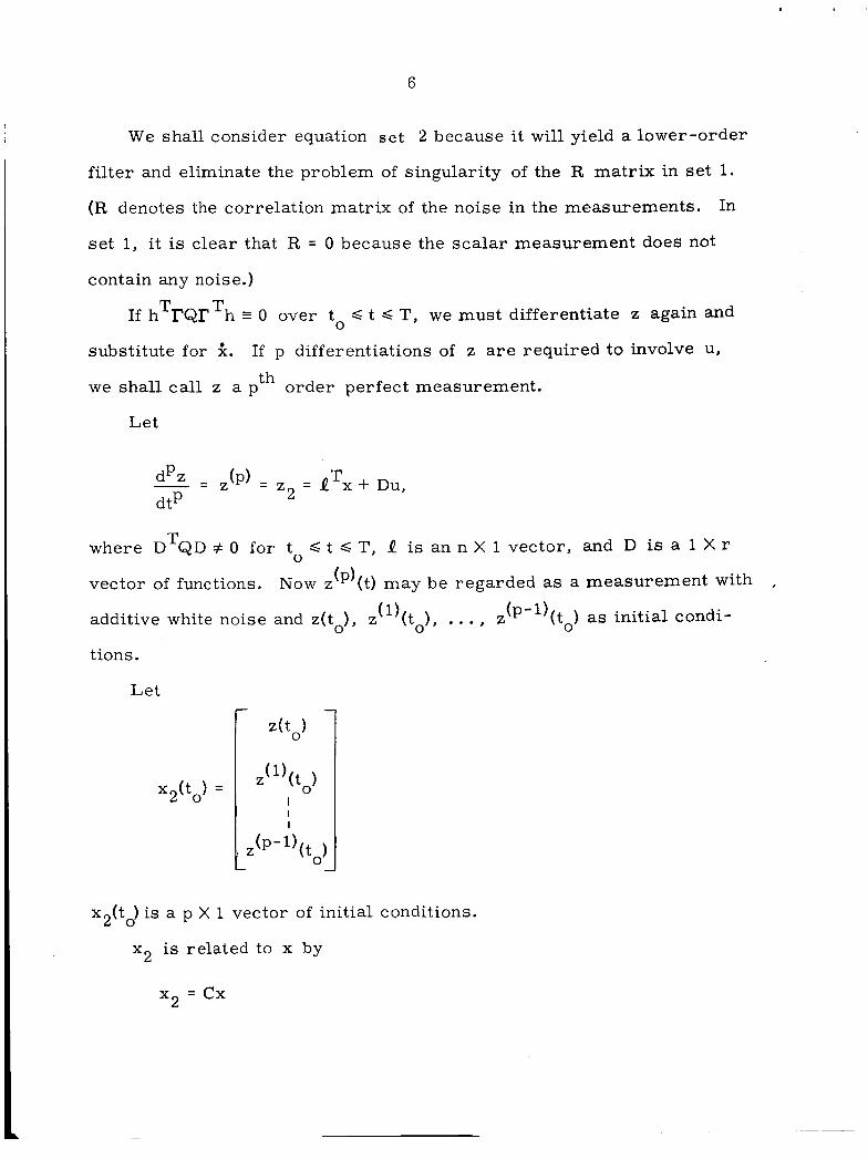
We shall consider equation set 2 because it will yield a lower-order
filter and eliminate the problem of singularity of the R matrix in se t 1.
(R denotes the correlation matrix of the noise in the measurements. In
se t 1, it is clear that R = 0 because the scalar measurement does not
contain any noise.)
T T - If h rQI' h = 0 over to S t S T, we must differentiate z again and
substitute for 5.
we shall call z a pth order perfect measurement.
If p differentiations of z a r e required to involve U,
Let
(p) = = QTx + Du, z 2 - - - z dp z dtP
T where D QD # 0 for to S t S T, Q is an n X 1 vector, and D is a 1 X r
vector of functions. Now z(P)(t) may be regarded a s a measurement with
additive white noise and z(to), z (1) (to), . . . , z (p-')(t0) as initial condi-
,
tions.
Let
x2(to) =
x2(tJ is a p X 1 vector of initial conditions.
x2 is related to x by
x2 = c x
7
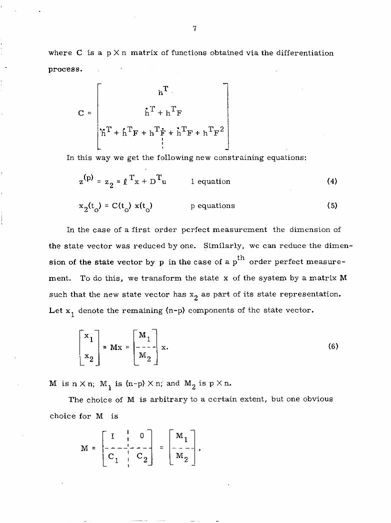
where C is a p X n matrix of functions obtained via the differentiation
process .
I C =
hT
AT + hTF
IbfiT+ ATF + hTk + kTF + h T 2 F
1 In this way we get the following new constraining equations:
1 equation (4) z ( ~ ) = z2 = QTx + D T u
X2(t0) = a t o ) x(to) p equations ( 5)
In the case of a f i r s t order perfect measurement the dimension of
the s ta te vector was reduced by one.
sion of the state vector by p in the case of a pth order perfect measure-
ment. To do this, we transform the state x of the system by a matrix M
such that the new state vector has x2 as part of i t s state representation.
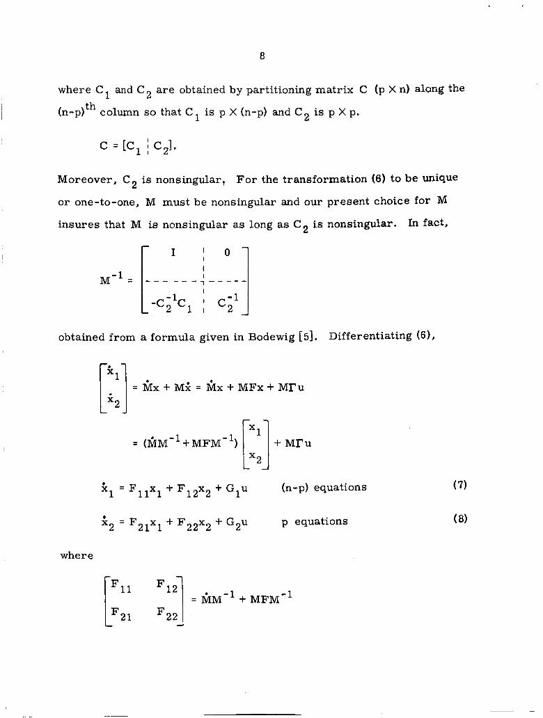
Let x denote the remaining (n-p) components of the state vector.
Similarly, we can reduce the dimen-
1
rl] = Mx =
M is n X n; MI is (n-p) X n;' and M2 is p X n.
The choice of M is arbi t rary to a certain extent, but one obvious
choice for M is
8
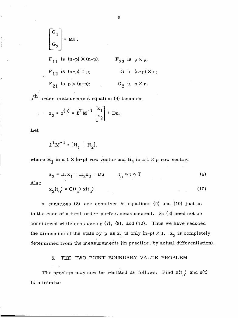
where C1 and C 2 a r e obtained by partitioning matrix C (p X n) along the
(n-p) th column so that C is p X (n-p) and C 2 is p X p.
c = [cl I czl.
Moreover, C2 is nonsingular, For the transformation (0) to be unique
o r one-to-one, M must be nonsingular and our present choice for M
insures that M is nonsingular as long as C2 is nonsingular. In fact,
obtained from a formula given in Bodewig [SI. Differentiating (6))
2 = F x + F 1 2 x 2 + G 1 u (n-p) equations 1 11 1
G 2 = FZlxl + F 2 2 ~ 2 + G2u p equations
where
9
is (n-p) X (n-p); is p x p ; *11
F12 is (n-p) X p;
is p X (n-p); F21
G is (n-p) X r;
G2 is p X r.
pth order measurement equation (4) becomes
Let
QTM-l = [H1 I H21,
where H is a 1 X (n-p) row vector and H2 is a 1 X p row vector. 1
(9) t s t s r 0
z2 = H x + H2x2 + Du 1 1 Also
x2(to) = a t o ) x(to). (10)
p equations (8) are contained in equations (9) and (10) just as
So (8) need not be in the case of a first order perfect measurement.
considered while considering (7), (9), and (10). Thus we have reduced
the dimension of the state by p as x1 is only (n-p) X 1.
determined f rom the measurements (in practice, by actual differentiation).
x2 is completely
5. THE TWO POINT BOUNDARY VALUE PROBLEM
The problem may now be restated a s follows: Find x(to) and u(t)
to minimize
10
b 0
subject to
= F l l x l + F x +G1u
= H x + H x + D u
12 2 t 4 t S T
;1 0
22 1 1 2 2
and
x2(to) = a t o ) x(to)
(n-p) equations (7)
1 equation (9)
p equations (10)
Note that the las t two equations together imply
for t S t C T . 0 x2(t) = C(t) x(t)
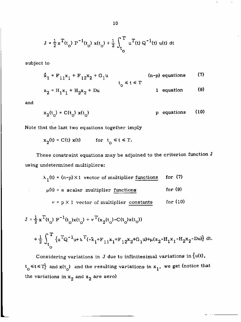
These constraint equations may be adjoined to the cr i ter ion function J
using undetermined multipliers:
.A ,(t) = (n-p) X 1 vector of multiplier functions for (7)
p(t) = a scalar multiplier functions for (9)
v = p X 1 vector of multiplier constants for (10)
T T + 3 I+ {uTQ-’u+ X (-%l+F l ~ l + F 12~2+G1~)+p(z2 -H1~1 -H2x2-Du)} dt.
b 0
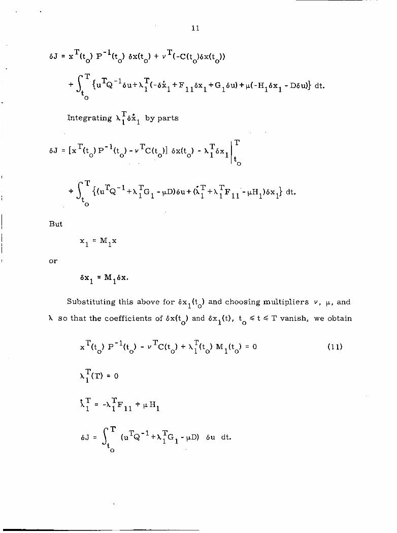
Considering variations in J due to infinitesimal variations in { d t )
toGtb’I’] and x(to) and the resulting variations in x l , we get (notice that
the variations in x2 and z2 are zero)
11
r r + {U'Q-~~U+X~ ( -6$l+F116~1+G16~)+p(-H 1 1 6x - Dbu)) dt.
0
r Integrating X 6gl by par ts 1 ~
65 = [x r (to) P-'(to) -vrC(t )] 6x(to) - X 1 r 6x1 0
* T T T + 1 {(uTQ-l +XTG1 - p,D)6u+ (A1 + A 1 Fll - pH1)6x1) dt.
L 0
I But
I x1 = M1x ~
or
6x1 = Mldx.
Substituting this above for 6x1(to) and choosing multipliers v , p,, and
A s o that the coefficients of 6x(to) and 6xl(t), to G t G T vanish, we obtain
k: = - X I F l l r + pHl
1 2
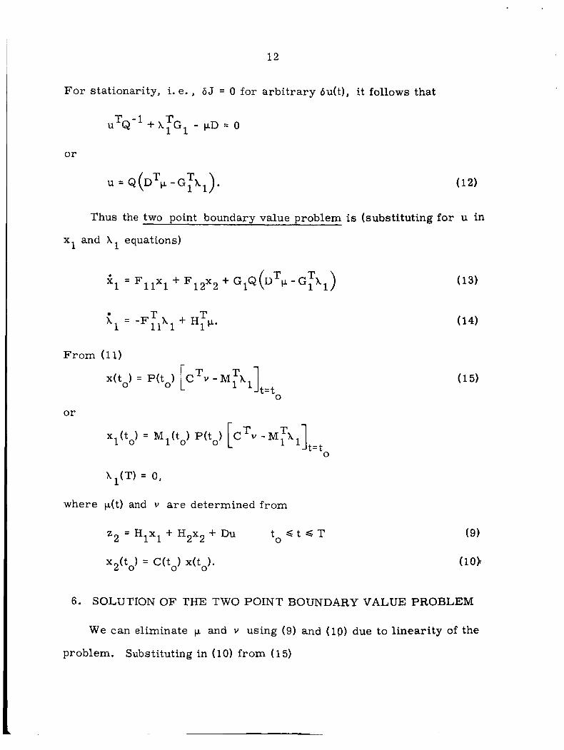
We can eliminate p and v using (9) and (10) due to l inearity of the
problem. Substituting in (10) f rom (15)
L
F o r stationarity, i. e . , 6J = 0 for a rb i t ra ry 6u(t), it follows that
o r
Thus the two point boundary value problem is (substituting for u in
x1 and X1 equations)
r r X1 = -F A + H1p. 11 1
F rom (11)
x(to) = P(to) [CTv - h ' I T A 1 ] t=to
or
Al(T) = 0,
where p(t) and v a r e determined from
t S t S T 0
= H x + H2x2+ Du z 2 1 1
x2(to) = a t o ) x(to).
(1 5)
6. SOLUTION OF THE TWO POINT BOUNDARY VALUE PROBLEM
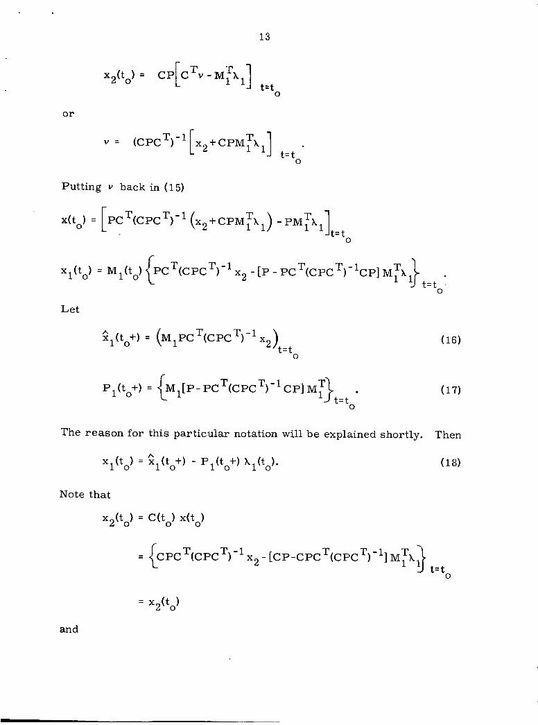
13
or
v =
0
Putting v back in (15)
' I t= to x(to) = [PCT(CPC T ) -1 (x2+CPM1X1) T -PMIX1
Let
fil(to+) = (MIPCr(CPC T ) -1 x2
0
P1(to+)
The reason for
xl(to) =
xz(to) =
Note that
= {Ml[P-PCT(CPC r ) -1 CP] M1 T}t=t 0
this particular notation will be explained shortly.
h Xl(t0+) - P1(to+) X1(to)*
(16)
(17)
Then
(18)
0
{CPCT(CPC
and

14
P ( t +) = {P -PCT(CPC r 1 -1
0 0
AS pointed out in [3], there is a simple explanation for these results
in te rms of the single stage estimation theory.
ments x2(to) become available at (to+), we update our estimate of the
state to %(to+) and the covariance matrix is correspondingly updated
to P(to+).
at time t = t
As soon as the measure-
Thus there a r e discontinuities in the state of the optimal fi l ter
0'
Now let us eliminate p f rom equations (13) and (14) using (9). Sub-
stituting u from (12) in (g),
T r z 2 = Hlxl + H2x2 + DQ (D p - G1 A l )
o r
T p. = (DQDT)-' (z2 - Hlxl - H2x2+ DQGl A , )
Putting this in ( 1 3 ) , (14), we get
-HIR r -1 H1 -
-G,QG;+G~QD r R -1 DQG, r
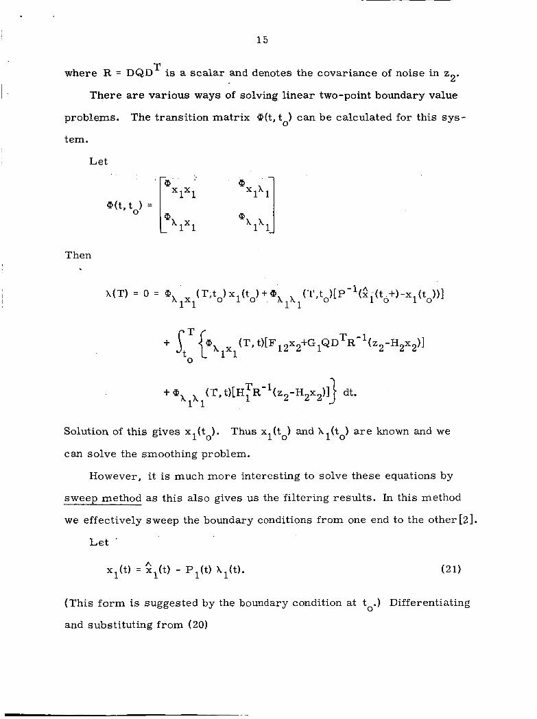
1 5
r where R = DQD is a scalar and denotes the covariance of noise in z2.
There are various ways of solving linear two-point boundary value
problems. The transition matrix Q(t, to) can be calculated for this sys-
tem.
Let
Q(t, to) =
- 1x1
Then 4
T -1 +@All1 (T, t)[H1 R
Solution of this gives xl(to).
can solve the smoothing problem.
Thus xl(to) and Xl ( to ) are known and we
However, i t is much more interesting to solve these equations by
sweep method as this also gives us the filtering results. In this method
we effectively sweep the boundary conditions from one end to the other [2].
Let
(This form is suggested by the boundary condition at to.) Differentiating
and substituting from (20)
16
T -1 T -1 T -1 (Fll-GIQD R H1)g1+F12x2+G1QD R (z2-H2x2) -Il -PIHIR H1”X1
= [.-&l+PIF~l-PIH1 T R -1 DQGT+GIQG~-GIQD r R -1 DQG1+FI1P1 T
-GIQD T R -1 HIP1-PIVIR T -1 H1Pl] h l o
Setting the coefficient of h l equal to zero,
= P ~ F E + F ~ ~ P ~ + G ~ Q G T - ( P ~ H ~ T + G ~ Q D T $1
Let
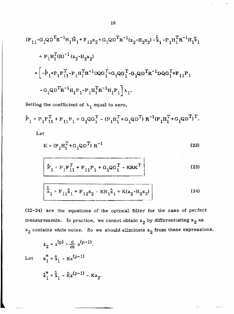
K = ( P ~ H : + G ~ Q D ~ ) R - ~ (22)
A = F x + F 1 2 x 2 - KH 2 + K(z -H X ) 1 5 1 11 1 1 1 2 2 2 I .._ I
(22-24) a r e the equations of the optimal f i l ter for the case of perfect
measurements. In practice, we cannot obtain z2 by differentiating x2 as
z2 contains white noise. So we should eliminate z 2 f rom these expressions.
Let x1 * A = x1 - Kz (p- 1)
17
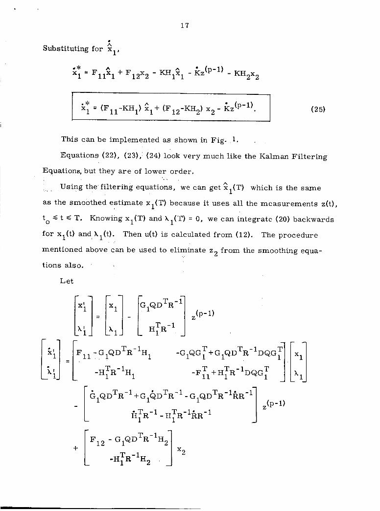
0 A Substituting for xl ,
m* A x1 = F x + F12x2 - KH1^xl - - KH2x2 11 1
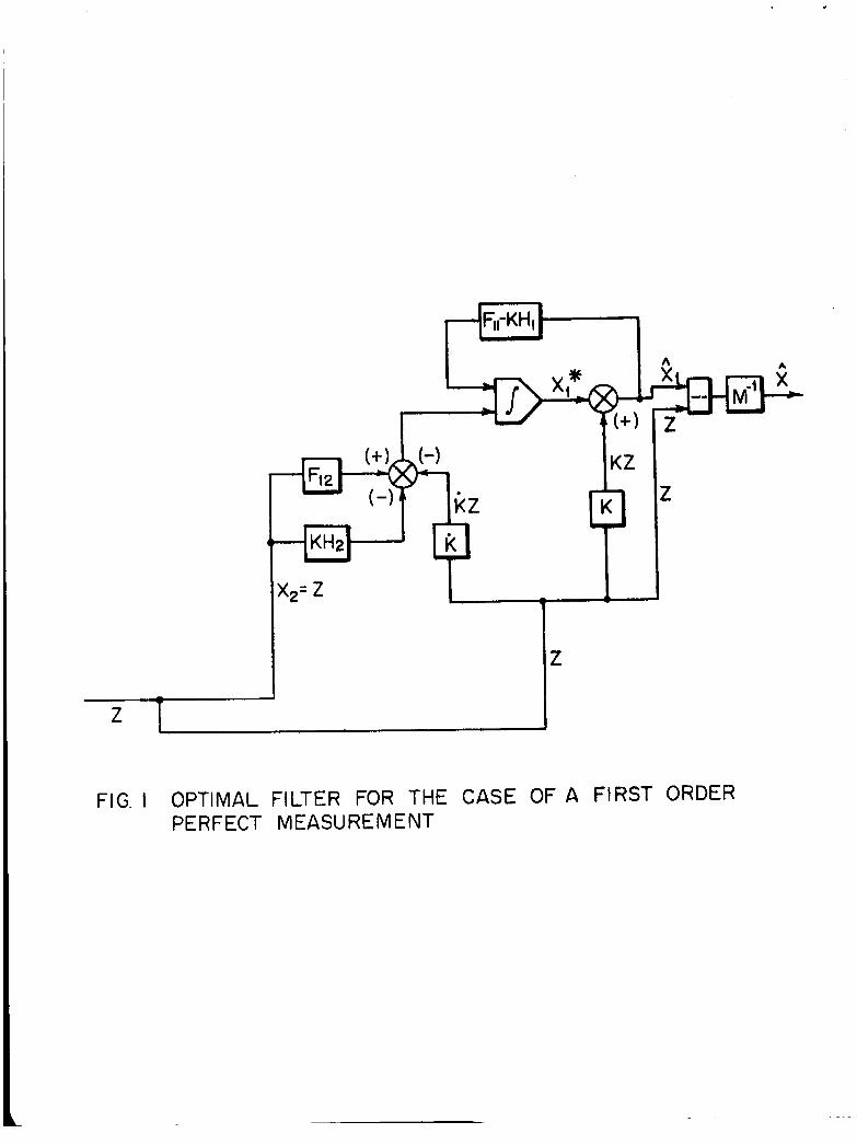
This can be implemented as shown in Fig. 1. . ,
Equations (22) , (231, (24) look very much like the Kalman Filtering
Equations, but they a r e of lower order. . .
Using the filterihg equations, we can get hxl(T) which is the same , .
I
I I
I
as the smoothed estimate x l ( T ) because it uses all the measurements d t ) ,
Knowing xl(T) and k l (T) = 0, we can integrate (20) backwards I t ,< t ,< T.
for xl(t) and Ll(t).
mentioned above can be used to eliminate z2 from the smoothing equa-
tions also.
0
Then u(t) is calculated from (12). The procedure
Let
T -1 -GIQD R H1
- H I R T -1 H1 -Fll T + H1 T R -1 DQGl T
(p- 1)
+ [*12
- G , Q D ~ R - ~ H , 1 x2 -HIR T -1 H2 .
+J - KH2 + x,= z
Z
L
Z
FIG. I OPTIMAL FILTER FOR THE CASE OF A FIRST ORDER PERFECT MEASUREMENT
n C l
c x I
19
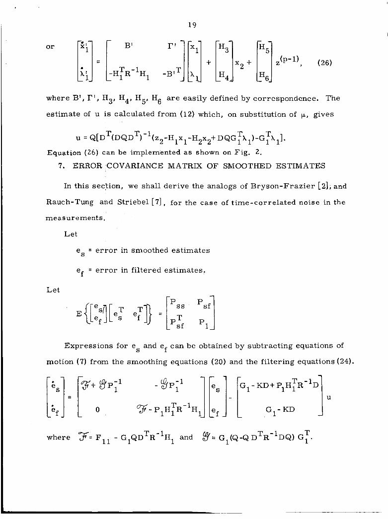
or
I = I
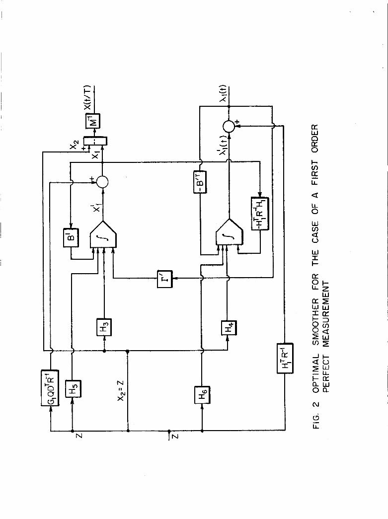
where B', I", Hg, H4, H5, H6 a r e easily defined by correspondence. The
estimate of u is calculated from (12) which, on substitution of p, gives
u =Q[D T (DQD T ) -1 ( z ~ - H ~ x ~ - H ~ x ~ + D Q G ~ X ~ ) - G ~ X ~ ] . r T
Equation (26) can be implemented as shown on Fig. 2.
7. ERROR COVARIANCE MATRIX OF SMOOTHED ESTIMATES
In this sec'tion, we shall derive the analogs of Bryson-Frazier [2], and
Rauch-Tung and Striebel [ 71, for the case of time-correlated noise in the
measurements . Let
= e r r o r in smoothed estimates eS
ef = e r r o r in filtered estimates.
Let 1
Expressions for e and ef can be obtained by subtracting equations of S
motion (7) from the smoothing equations (20) and the filtering equations (24).
2 1
3
Q(G~-KD+PH~R T -1 .> T ,
a
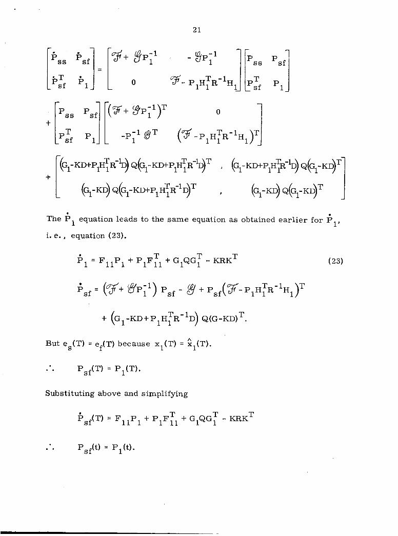
The P
i. e . , equation (23) .
equation leads to the same equation as obtained ear l ier for P1, 1
T -n -n p1 = F P + P ~ F ; ~ + G ~ Q G ; - K R K ~ 11 1
= (%+ $I?;') P sf - 8 + P s f ( F - P I H I R T -1 Hl)'
+ ( G ~ - K D + P ~ H ~ T R -1 D) Q ( G - K D ~
A But e (T) = e (T) because xl (T) = xl(T).
. . Psf(T) = P1(T).
Substituting above and simplifying
S f
. . PsfW = Pl(t) .
2 2
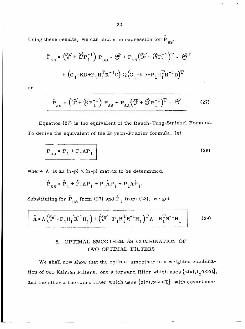
Using these results, we can obtain an expression for P ss'
0
= ("3;. 9P;') P - g? + Pss(%+ 3 P l -1)T- $y pss ss
or
Equation (27) is the equivalent of the Rauch- Tung-Striebel Formula.
TO derive the equivalent of the Bryson-Frazier formula, let
I------l lPss = P1 + P I A P l I
where A is an (n-p) X (n-p) matrix to be determined.
. = 6, + 6 , A P 1 + P1ilP1 + PIAf'l-
Substituting for FSs frow (27) and 6, from (23) , we get
A = A ( C ~ ; - P ~ H ~ R T -1 H ~ ) + ( T ' - P ~ H ~ R T -1 H ~ ) ~ A - H ~ T -1 H~
-_ ---
8. OPTIMAL SMOOTHER AS COMBINATION OF TWO OPTIMAL FILTERS
(28)
We shall now show that the optimal smoother is a weighted combina-
tion of two Kalman Fi l ters , one a forward fi l ter which uses {z(a),toGaCt)J
and the other a backward fi l ter which uses {z(a),tCa GT} with covariance
23
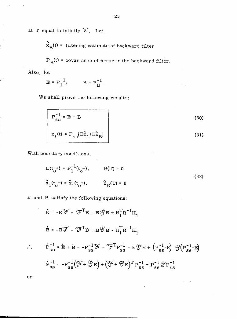
at T equal to infinity.[8]. Let
h xB(t) = filtering estimate of backward filter
P (t) = covariance of e r r o r in the backward filter. B
Also, let
B = P B . -1
We shall prove the following results:
P-l = E + B ss
xl(t) = Pss[E$l+B$B] (31)
With boundary conditions
E(to+) = Pi1(t0+),
Xl(t0+) = x1(t0+),
B(T) = 0
xB(T) = 0
E and B satisfy the following equations:
A A A
k = -ET - T ~ E - E YE + H~ T R -1 H~
h = - B y - T T B + B # B - H I R T -1 H1
. . i . - l = k + = -p-1% - q T p - l - E ~ E + (.-'-E) Y(P~;-E) ss ss ss s s
pss ' -' = -Pel(%+ ss YE) + (5. $?E)TPi: + Pi: c$?P~:
or
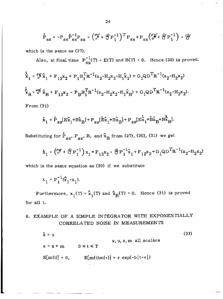
24
= -P P -1 P = (F+$Pl -1 ) T pss+pss pSS ss ss ss
which is the same as (27).
Also, at final time PBi(T) = E(T) and B(T) = 0. Hence (30) is proved.
T -1 A T -1 x1 = yGl + F 1 2 x 2 + P I H I R (z2-H2x2-HlhX1) + GIQD R (z2-H2x2)
T -1 T -1 A ;B=%;;B+F12~2 - P H R (z2-H2x2-H1GB) + GIQD R (z2-H2X2).
F rom (31)
r\ ' A A k1 = 6ss[EQ1+BhXB] + Pss[k$l+BgB] + Pss[Exl+BxB+BxB].
Substituting for fiSs, Pss, B, and ^xB from (27), (30), (31) we get
T -1 x1 = (v+ @Pi1)x1+F12x2 - $P;'k1+Fl2x2+G1QD R (z2-H2x2)
which is the same equation as (20) i f we substitute
-1 A h l = P1 (X -X ). 1 1
A Furthermore, xl(T) = xl(T) and GB(T) = 0. Hence (31) is proved
for all t.
9. EXAMPLE OF A SIMPLE INTEGRATOR WITH EXPONENTIALLY
CORRELATED NOISE IN MEASUREMENTS
. (33) x = u x J u J z , m all s ca l a r s
z = x + m O S t S T
E[m(t)l = 0, E [ m ( t ) m ( ~ ) ] = r exp(-b I t-7 1 )

m(t) can be produced by passing white noise through a f i rs t order filter.
= -bm + bw
where
E[w(t)l = 0,
E[m<O>l = 0,
E[ W(t)W(7)] 2 r 6(t-T)
E[m (011 = r. 2
There is no correlation between u(t), w(t), x(O), and m(0). In this
problem, the augmented state equations a r e
[:I = [: -:][:I + [buw]
0 . z = x + rh = u - bm + bw = u - b(z-x) + bw or
- . . x2 = z and z2 - d .
Equation (33) corresponds to equation (7).
D = [ l , 13, H1 = b, H2 = -b
2 T
R' R = DQD = q + 2rb;
26
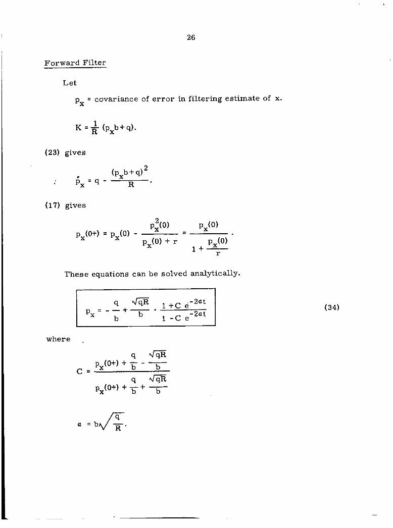
Forward Filter
Let
p, = covariance of e r r o r in filtering estimate of x.
1
s e equations can be solved analytically.
1 -2at -2at
- q - 1 + c e
p x - -;+- I - C ~
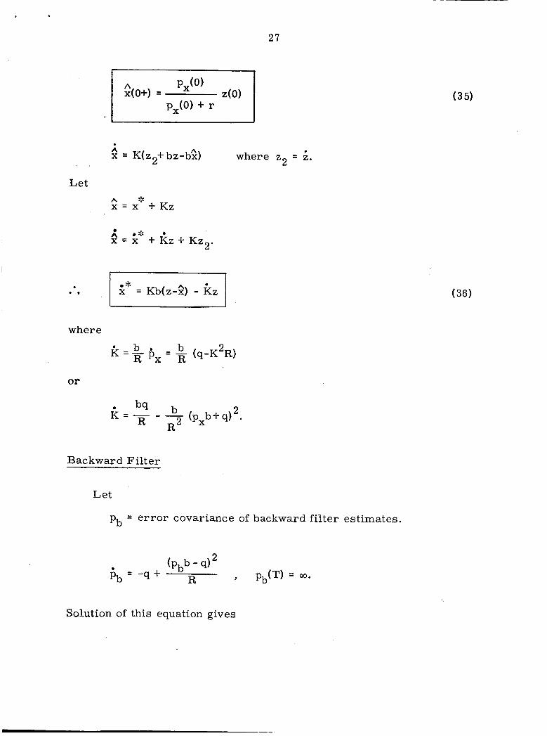
27
A x = K(z2+ bz-b?) where z2 = k.
Let n x = xl’ + Kz
b $ b c = x + K z + K z 2 .
. .
where
or
Backward Filter
Let
pb = e r ro r covariance of backward filter estimates.
Solution of this equation gives
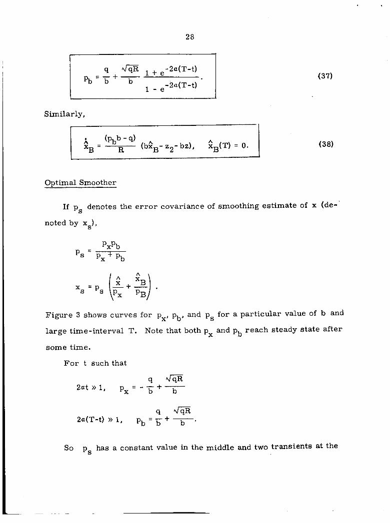
28
q &p + e-2a(T-t) - - + -
b - 2a( T - t) pb - b 1 - e
(37)
Similarly ,
I
Optimal Smoother
If ps denotes the e r r o r covariance of smoothing estimate of x (de-'
noted by xS)'
Figure 3 shows curves for p,, pb, and p, for a particular value of b and
large time-interval T. Note that both px and pb reach steady state after
some time.
For t such that
- s a - - - + - b b 2at >> 1, px
so ps has a constant value in the middle and two transients at the
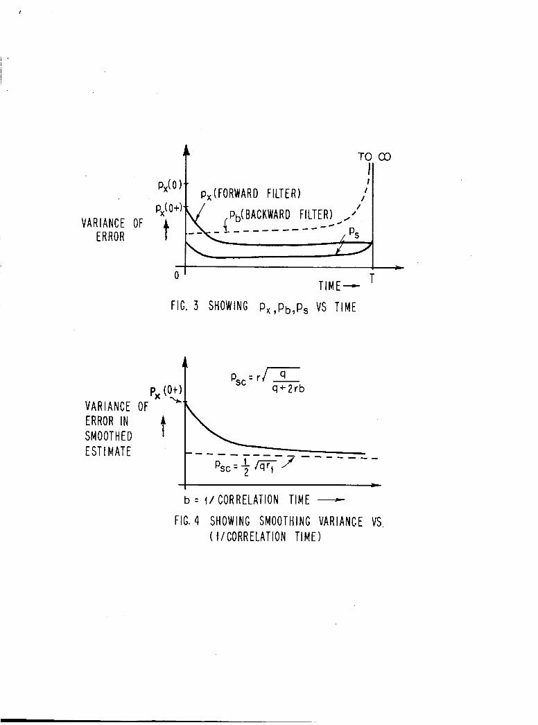
TO 03 II
V A R I A N C E ERROR
OF
px(o)t p,(FORWARD F I L T E R )
I - 0 ' T T I M E -
FIG. 3 SHOWING P,,Pb,Ps VS T I M E
= r n - PSC 4 + 2 r b Px (O+) I. V A R I A N C E OF
ERROR I N SMOOTHED E S T 1 M A T E - - - - - ----- - - - - - - -
t P,, = + /4rl f
1 -
b = I / CORRELATION T I M E - FIG. 4 SHOWING SMOOTHING V A R I A N C E VS.
( i / C O R R E L A T I O N T I M E )
30
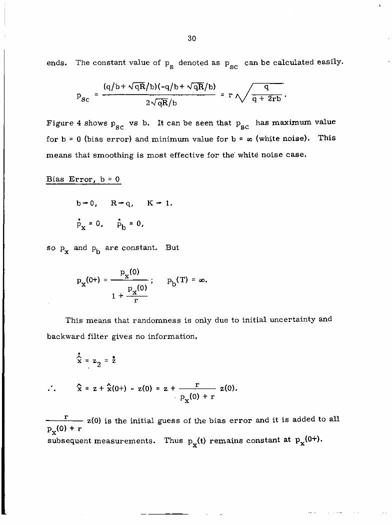
ends. The constant value of p, denoted as psc can be calculated easily.
Figure 4 shows psc vs b,
for b = 0 (bias e r r o r ) and minimum value for b = 00 (white noise).
means that smoothing is most effective for the' white noise case.
It can be seen that psc has maximum value
This
Bias E r r o r , b = 0
b-0, R-q, K - 1.
= O, & =
so p, and pb a r e constant. But
This means that randomness is only due to initial uncertainty and
backward filter gives no information.
b A
=. z2 =
z(0) A r . . x = 2 + $(O+) - z(0) = z + PX(O) +
z(0) is the initial guess of the r
px(0) + r subsequent measurements. Thus p,(t)
r
bias e r r o r and i t is added to all
remains constant at p,(O+).

31
It is clear that for this case, smoothing estimates a r e exactly the A
same as filtering estimates. ps - - p,; xs = x. So we do not gain anything
by smoothing the results.
2 r White Noise, b - 06 and - b - rl rl is the a rea under the delta function representing spectral dens’ity
of white noise m(t).
where
A PX x(O+) = 0, K - 0 but Kb- -
. . . A px A x = -(z-x).
32
This is the usual Kalman Filter. For the backward filter,
The asymptotic values of pb and p, a r e the same, viz. , 6. 1 . . Ps, = T"ss'l*
For constant values of p,, the smoothing estimate is the mean of the
filtering estimates
A A x + XB 2 ' x = S
10. GENERAL CASE
For the general case, manipulations get very involved, but the resul ts
W e shall only s ta te the problem and give the final are essentially similar.
results . Augmented state and measurement equations are
z1 = H 1 x + w
y = c x ,
where
3 3
z1 = q X 1 vector of measur.ements containing white noise
y = r X 1 vector of perfect measurements
w = q X 1 vector of white noise e r r o r s in z 1
E{u(t)} = 0;
E{w(t)} = 0;
E{u(t)uT(T)} = Q(t) 6(t--r)
E{w(t)w'(T)} = Rl(t) b(t-T)
E(u(t)w'(t)} = sl ( t ) ; E{x(to)} = 0; E{x(to)x T (to)} = P(to)
E{w(t)xT(to)} = 0.
I , The smoothing problem can be stated as follows: Minimize
subject to
$ = F x + r u
y = cx.
Filtering results obtained a r e
b 7- n -n
P I = F P + P ~ F ; ~ + G ~ Q G ; - K ~ R K ~ 11 1
b
= F 2 + F x + K 1 ( z - d l ) 1 11 1 1 2 2
where
34
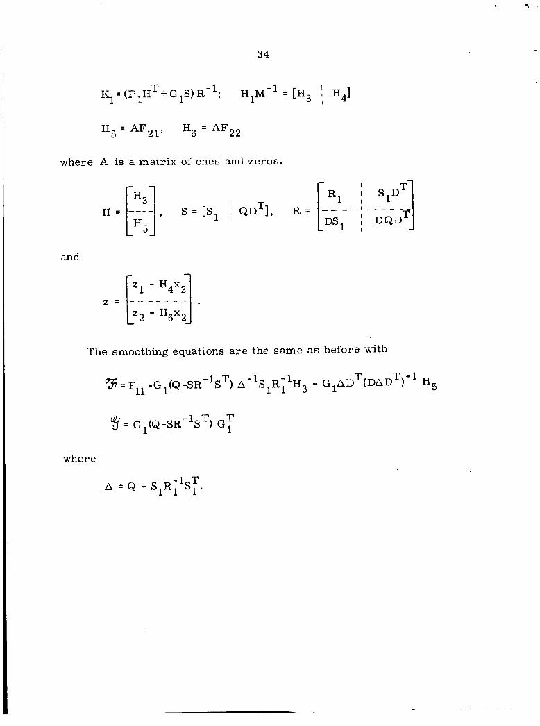
r I K1=(PIH +GIS)R-l;
H5 = AFZ1,
H1M-' = [H3 I I H4]
Hg = AF22
where A is a matrix of ones and zeros.
s = [sl I I I QDTl,
I
DS1 I I
and
The smoothing equations a r e the same as before with
T -1 "3; = Fll -G1(Q-SR -1 S T ) A-lS1RT1H3 - G , A D ~ ( D A D ) H~
-1 T T 3= G1(Q-SR S ) GI
where
35
REFERENCES
[l] Kalman, R. E . , and R. S. Bucy, !!New Results in Linear Filtering and Prediction Theory,ll ASME Trans. (J. of Basic Engineering), Vol. 83D, March 1961, pp. 95-108.
[2 ] Bryson, A. E. , and M. Fraz ie r , llSmoothing for Linear and Non- linear Dynamic Systems,I1 Proc. of the Optimum Systems Synthesis Conf., U. S. Air Force Technical Report ASD-TDR-063-119, February 196 3.
[3] Bryson, A. E . , and D. E. Johansen, "Linear Filtering for Time- Varying Sys tems Using Measurements Containing C oloured Nois e, IEEE Trans. on Automatic Control, January 1965.
[4] Ho, Y. C . , and R. C.Lee, Stochastic Estimation and Control, It IEEE Transactions on Automatic
Bayesian Approach to Problems in
Control, Vol. AC-9, No. 4, October 1964.
[ 51 E. Bodewig, Matrix Calculus, North-Holland Publishing Co., Amsterdam; Interscience Publishers, Inc. , New York, 1956.
[6] Bryson, A. E., and Y. C. Ho, IlOptimal Programming, Egtimation and Control,11 Lecture Notes, Harvard University, 1966-1967.
[7] Rauch, Tung, and Striebel, ltMaximum Likelihood Estimates of Lin- e a r Dynamic Systems,11 AIAA Journal, Vol. 3, No. 8, pp. 1445- 1450, August 1965.
[8] F r a s e r , Donald C . , "On the Application of Optimal Linear Smoothing Techniques to Linear and Nonlinear Dynamic Systems,lI Ph. D. Thesis, Massachusetts Institute of Technology, January 196 7.
[ 9 ] A . E. Bryson and S R. McReynolds, "A Successive Sweep Method for Solving Optimal Programming Problems, I ' Sixth JACC, Troy, N. Y. , June 1965.