Smoke plume height measurement of prescribed burnsin the south-eastern United States

Yongqiang LiuA,B, Scott L. GoodrickA, Gary L. AchtemeierA, Ken ForbusA

and David CombsA

AUSDA Forest Service, Center for Forest Disturbance Science, 320 Green Street,

Athens, GA 30602, USA.BCorresponding author. Email: yliu@fs.fed.us

Abstract. Smoke plume height is important formodelling smoke transport and resulting effects on air quality. This study

presents analyses of ceilometer measurements of smoke plume heights for twenty prescribed burns in the south-easternUnited States. Measurements were conducted from mid-winter to early summer between 2009 and 2011. Approximatelyhalf of the burns were on tracts of land over 400 ha (1000 acres) in area. Average smoke plume height was,1 km. Plume

height trended upward from winter to summer. These results could be used as an empirical guideline for fire managers toestimate smoke plume height in the south-eastern US when modelling and measurement are not available. The averagecould be used as a first-order approximation, and a second-order approximation could be obtained by using the average forspring and autumn seasons, and decreasing or increasing by 0.2 km the average for winter or summer. The concentrations

of particulate matter with an aerodynamic diameter less than 2.5 or 10 mm (PM2.5 and PM10) within smoke plumescalculated from ceilometer backscatter are,80 and 90 mgm�3, and trend downward fromwinter to summer. Large smokeconcentrations are found in the lower portion of smoke plumes for many burns. Smoke plume height shows fast and

uniform fluctuations at minute scales for almost all burns and slow and irregular fluctuations at scales from tens ofminutesto hours for some burns.

Additional keywords: ceilometer measurement, particulate matter concentration.

Received 19 May 2011, accepted 16 July 2012, published online 24 September 2012

Introduction

Smoke plume height (also known as smoke plume rise, or smokeplume final rise in some early studies) is the height wherevertical ascent of a smoke plume ceases. Smoke plume heights

range from hundreds of metres for prescribed fires to thousandsof metres for wildfires. Plume height is an important factor forlocal and regional smoke transport and air-quality modelling.

Fire emissions, if injected to higher elevations, can be trans-ported out of rural burn sites to affect air quality at distant highlypopulated urban areas. Smoke plume height is a required inputfor many regional air-quality models. The Community Multi-

scale Air Quality (CMAQ) model (Byun and Ching 1999; Byunand Schere 2006), for example, uses the Sparse Matrix OperatorKernel Emissions (SMOKE) modelling system (Houyoux et al.

2002) to provide plume height as part of initial and boundaryconditions for elevated emission sources. The BlueSky wildfiresmoke modelling system (Larkin et al. 2009) also includes

algorithms for smoke plume height calculation in order todetermine the downwind smoke concentrations and effects onair quality.

In the early smoke modelling applications of CMAQ andSMOKE, the Briggs scheme (Briggs 1975) was used to calculatesmoke plume height. The Briggs scheme (Briggs 1975) is a two-thirds power law integral model based on differential equations

governing mass, momentum and energy fluxes through a plume

cross-section (Weil 1988). The calculated plume height isdetermined by both emission properties, such as initial buoyancyflux and exit velocity, and ambient properties, such as wind and

thermal stability. The two-thirds power law is formulated on theassumption that plume buoyancy flux dominates plumemomen-tum flux (not the ambient mechanical turbulence), thus in theory

if the plume momentum flux dominates, the formula will notperform well. Guldberg (1975) compared the accuracy of theBriggs scheme (Briggs 1975) with two other schemes in model-ling the heights of hot, buoyant plumes and found that the Briggs

scheme (Briggs 1975) best predicted the observed plume heightsduring periods of low wind speed.

In comparison with a single power plant stack, on which the

Briggs plume rise scheme (Briggs 1975) is based, forest burninghas multiple-core plumes, which are usually more buoyant andinvolve stronger atmospheric entrainment. In addition, mechan-

ical turbulence generated at the ground surface can be of similarmagnitude to the buoyantly produced turbulence for weak forestfires, especially a prescribed burn under windy conditions.

These differences lead to potential problems with the applica-tion of the Briggs scheme (Briggs 1975) to fire smoke plumeheight modelling. For example, the National Oceanic andAtmospheric Administration’s Smoke Forecasting System

CSIRO PUBLISHING

International Journal of Wildland Fire

http://dx.doi.org/10.1071/WF11072

Journal compilation � IAWF 2012 www.publish.csiro.au/journals/ijwf

showed a tendency to over-predict the measured PM2.5 (partic-ulate matter with an aerodynamic diameter less than 2.5mm)concentrations in the western United States between September

2006 and November 2007 (Stein et al. 2009), and this predictionwas shown to be very sensitive to the injection height of fireemissions calculated using the Briggs scheme (Briggs 1975).

The problems with the Briggs scheme (Briggs 1975) for fireapplication emphasise the importance in developing smokeplume height schemes specifically for wildfires and prescribed

fires. Efforts have been made recently that led to the develop-ment of several smoke plume models with various levels ofcomplexity. Harrison and Hardy (2002) developed an empiricalmodel to estimate plume rise using maximum flame power

(power of a flame is a measure of the total radiative energyleaving the surface of the fire in unit time) based on themeasurement of a large number of prescribed burns in the

north-western United States (Hardy et al. 1993). Pouliot et al.(2005) modified the Briggs scheme (Briggs 1975) by convertingthe heat flux from each fire to a buoyancy flux suitable for use

with the Briggs plume rise algorithm (Briggs 1975). TheWestern Regional Air Partnership (Western Regional AirPartnership 2005) used a climatological method by specifying

pre-defined plume bottom and plume top and a pre-defineddiurnal temporal profile for each fire. The modified Briggsscheme (Briggs 1975) and the WRAP climatological methodhave been incorporated into SMOKE. Freitas et al. (2007)

developed a model to explicitly simulate smoke plume heightbased on a one-dimensional dynamic entrainment plume model(Latham 1994). It was modified later to include the effects of

winds (Freitas et al. 2010). An extended set of equations,including the horizontal motion of the plume and the additionalincrease of the plume size, was solved to explicitly simulate the

time evolution of plume height and determine the final injectionlayer. This model has been incorporated into the WRF-Firemodelling system and evaluated for individual wildfire events(Grell et al. 2011; Mandel et al. 2011). WRF-Fire combines the

Weather Research and Forecasting (WRF) model (Skamarocket al. 2008) with a surface fire behaviour model for calculatingfire spread rate using fuel properties, wind velocities fromWRF,

and terrain slope.WRF-Fire allows modelling of the growth of awildland fire and the dynamic feedbacks with the atmosphere.

Prescribed burning is an important tool for forest andwildlife

management, including managing rare and endangered plantsand animals, while reducing the buildup of fuels and the risk ofdestructive wildfire. Approximately 2� 106–3� 106 ha

(6� 106–8� 106 acres) of forest and agricultural lands areburned each year in the southern United States (Wade et al.

2000). In comparison with wildfires, buoyancy generated byprescribed fires is smaller because there is typically less heat

released. Achtemeier et al. (2011) developed a dynamical-stochastic smoke plume model (Daysmoke) specifically forprescribed fires. Based on ASHFALL (Achtemeier 1998),

a plume model for deposition of ash from sugarcane fires,Daysmoke includes an entraining turret plume sub-model,a detraining particle trajectory sub-model, a convective circula-

tion parameterisation and an emissions production sub-model.Daysmoke has been incorporated into SHRMC-4S, a frameworkfor simulating smoke and air quality effects of prescribedburning (Liu et al. 2009).

Smoke plume measurement is essential for validating smokemodels. Several smoke detection techniques are available formeasuring smoke plume height. Weather radars such as the

Weather Surveillance Radar-1988 Doppler (WSR-88D) in theUS national network have historically been used to detect smokeplume reflectivity and structure (e.g. Banta et al. 1992; Rogers

and Brown 1997; Jones and Christopher 2008; Melnikov et al.

2008; Tsai et al. 2009). LiDAR (light detection and ranging) iswell adapted for smoke detection (e.g. Pershin et al. 1999;

Mikkelsen et al. 2002; Lavrov et al. 2003; Colarco et al. 2004;Muller et al. 2005). LiDAR emits laser beams and receivesbackscatter signals from smoke particles that can be processedto provide spatial and temporal variations of smoke concentra-

tions. LiDAR has the advantage of simplicity, low cost, equip-ment mobility, robustness and low energy consumption (Lavrovet al. 2006) and is amenable to several platforms: ground,

aircraft and satellite. Kovalev et al. (2009) stated that LiDARwas the most appropriate tool for ground-based monitoring ofwildfire smoke plume dynamics and heights at different down-

wind distances. There are two satellites that are capable ofdefining plume injection height: the Cloud-Aerosol LiDARwithOrthogonal Polarisation (CALIOP) aboard the Cloud-Aerosol

LiDAR and Infrared Pathfinder Satellite Observations(CALIPSO) satellite (Winker et al. 2006) and the Multi-angleImaging Spectroradiometer (MISR) aboard the US NationalAeronautics and Space Administration (NASA) Terra satellite

(Kahn et al. 2007, 2008; Labonne et al. 2007; Diner et al. 2008;Raffuse et al. 2009; Amiridis et al. 2010). Although thesesatellites have global coverage, the temporal frequency is low

(16 days for CALIOP and 9 days for MISR).Smoke plume height model evaluation for prescribed fires is

a challenge because of limited smoke plume height validation

data (Jones and Christopher 2008). This makes it difficult tounderstand the performance and uncertainties of smoke models.Fire and smoke model validation is one of the fundamentalresearch issues identified in the Smoke Science Plan (Riebau

and Fox 2010), prepared for the US Joint Fire Science Program(JFSP). The JFSP and the Strategic Environmental Research andDevelopment Program (SERDP) have supported several

research projects to collect smoke data for model validation.This paper presents results from smoke plume rise measure-ments of prescribed fires in the south-eastern US.

Methods

Burn sites

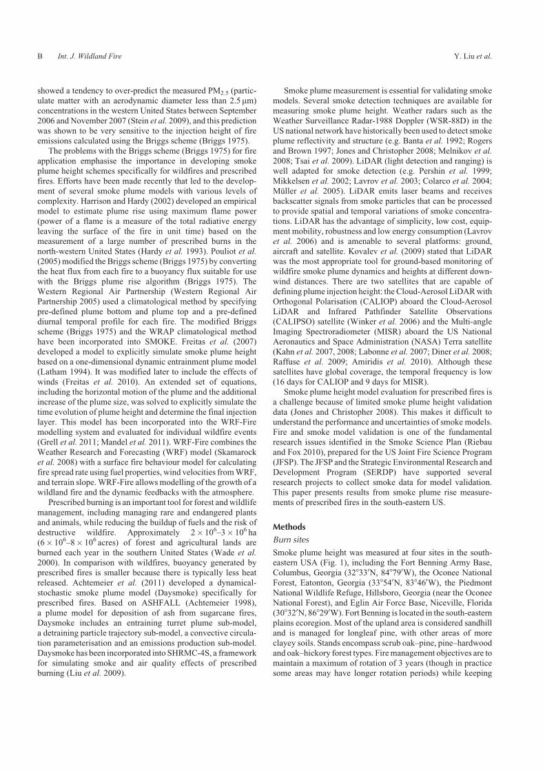
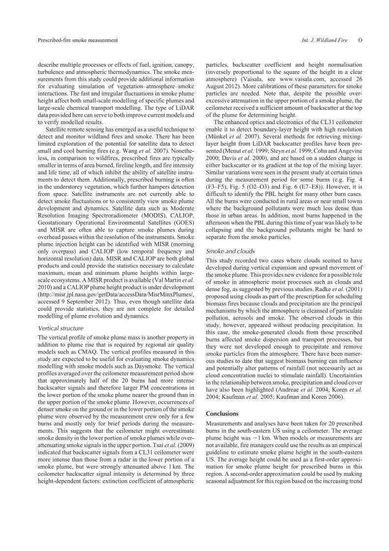
Smoke plume height was measured at four sites in the south-eastern USA (Fig. 1), including the Fort Benning Army Base,Columbus, Georgia (328330N, 848790W), the Oconee National

Forest, Eatonton, Georgia (338540N, 838460W), the PiedmontNational Wildlife Refuge, Hillsboro, Georgia (near the OconeeNational Forest), and Eglin Air Force Base, Niceville, Florida

(308320N, 868290W). Fort Benning is located in the south-easternplains ecoregion. Most of the upland area is considered sandhilland is managed for longleaf pine, with other areas of more

clayey soils. Stands encompass scrub oak–pine, pine–hardwoodand oak–hickory forest types. Firemanagement objectives are tomaintain a maximum of rotation of 3 years (though in practicesome areas may have longer rotation periods) while keeping

B Int. J. Wildland Fire Y. Liu et al.

smoke within the confines of the military base. All burns areground-ignition fires, conducted mostly during late winter and

early spring.The Oconee National Forest and the Piedmont National

Wildlife Refuge are located in the Piedmont region of Georgia,which lies between the Atlantic Coastal Plain and the Blue

Ridge Mountains. This region consists mostly of low hills andnarrow valleys. The majority of the forests is mixed, consistingprimarily of an overstorey of oak, hickory and pine. The

National Forest and the Refuge also have extensive areas ofalmost pure upland pine maintained by fire. The OconeeNational Forest plan is to burn between 4000 and 8000 ha year�1

(10 000 and 20 000 acres year�1) on a 3–5-year rotation.Because of the high fire return frequency, fuel loading isgenerally light and produces slow-burning fires with low flame

heights. The area, stand types and ignition methods varydepending on land-management objectives. Therefore, firebehaviour also varies. Large-area burns are usually conductedby backing fires through ground ignition to create black lines,

followed by aerial ignition.Eglin Air Force Base is located in the East Gulf Coastal Plain

ecoregion. A majority of habitats are fire dependent and main-

tained by one of the largest fire-management programs in thecountry. Most of the area is a sandhill ecosystem, which consistsof longleaf pine overstorey. The management goal of the

prescribed-fire program requires burning large tracts throughaerial ignition.

Detection device

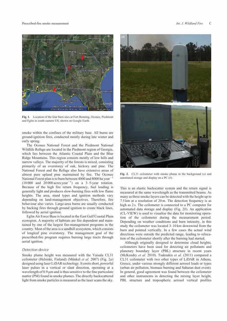
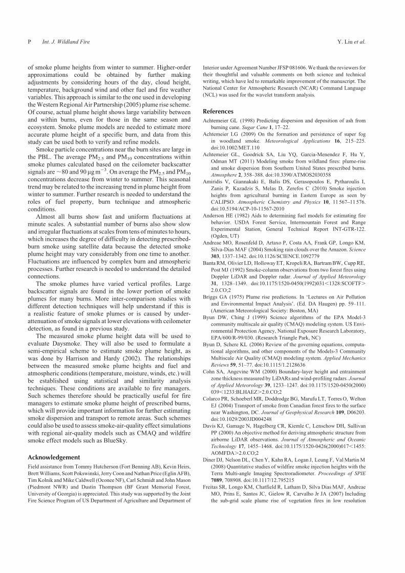
Smoke plume height was measured with the Vaisala CL31ceilometer (Helsinki, Finland) (Munkel et al. 2007) (Fig. 2a)designed using laser LiDAR technology. It emits short, powerfullaser pulses in a vertical or slant direction, operating at a

wavelength of 0.9 mm and is thus sensitive to the fine particulatematter (PM) found in smoke plumes. The directly backscatteredlight from smoke particles is measured as the laser scans the sky.

This is an elastic backscatter system and the return signal ismeasured at the same wavelength as the transmitted beams. Asmany as three smoke layers can be detected with the height up to

7.5 km at a resolution of 20m. The detection frequency is ashigh as 2 s. The ceilometer is connected to a PC computer forautomated data storage and display (Fig. 2b). An application(CL-VIEW) is used to visualise the data for monitoring opera-

tion of the ceilometer during the measurement period.Depending on weather conditions and burn intensity, in thisstudy the ceilometer was located 3–10 km downwind from the

burn and pointed vertically. In a few cases the actual winddirections were outside the predicted range, leading to reloca-tion of the ceilometer shortly after the burning had started.

Although originally designed to determine cloud heights,ceilometers have been used for detecting air pollutants andplanetary boundary layer (PBL) structure in recent years

(McKendry et al. 2010). Tsaknakis et al. (2011) compared aCL31 ceilometer with two other types of LiDAR in Athens,Greece, under various strongly different aerosol loads or types(urban air pollution, biomass burning and Saharan dust event).

In general, good agreement was found between the ceilometerand other instruments in detecting the mixing layer height,PBL structure and tropospheric aerosol vertical profiles

Fig. 1. Location of the four burn sites at Fort Benning, Oconee, Piedmont

and Eglin in south-eastern US, shown on Google Earth.

(a)

(b)

Fig. 2. CL31 ceilometer with smoke plume in the background (a) and

automated storage and display on a PC (b).

Prescribed-fire smoke measurement Int. J. Wildland Fire C

Tsai et al. (2009) measured a prescribed burn at Fort Benning in2008 using a CL31 ceilometer and a millimetre-wavelengthDoppler radar. Similar plume morphology existed in both

measurements; but the LiDAR backscatter was strongly attenu-ated above 1 km and the radar echo extended higher than theLiDAR signals. The laser light source used in ceilometers is less

powerful and spectrally broader than that of the radar; thus theability of ceilometers to detect aerosols is restricted to 3-kmheight or less (Markowicz et al. 2008).

Smoke concentration

PM2.5 and PM10 concentrationswere estimated from backscatterusing the following formula (Munkel et al. 2004, 2007):

CPM10¼ mbþ b ð1Þ

CPM2:5¼ 0:6846þ 0:8608� CPM10

ð2Þwhere CPM2.5

and CPM10are PM2.5 and PM10 concentrations, b is

the measured smoke backscatter coefficient and regressioncoefficients are m¼ 2.023� 107mgm�2 srad (solar radiation)and b¼�1.6304mgm�3.

Note that these formulae were obtained based on backscatterdata measured with a CT25KA ceilometer (a Vaisala ceilometerolder than that used in the present work). Further studies

incorporating a CL31 ceilometer for refinement and finalisationof this formula are required (Munkel et al. 2007). Furthermore,the formulae were developed based on the measurements of

pollutants at a low elevation (20m above the ceilometer loca-tion). Possible uncertainties in their applications to fire smokeplumes at much higher elevations are yet to be determined.

Wavelet transform

Wavelet transform was used to analyse temporal fluctuations ofthe measured smoke plume height. Smoke plumes rise in the

PBL, where turbulent motions often make it difficult to identifytemporal variability in smoke plume height. Spectral or signalanalysis techniques are needed to extract the variability. Similarto the Fourier transform, the wavelet transform, introduced by

Morlet et al. (1982a, 1982b), is a tool to extract cyclic infor-mation (various spectrum or scales, amplitude and phase) hid-den in a series, or to represent the series with certain-degree

filtering. However, unlike the Fourier transform, the wavelettransform is conducted in a scale-location domain (the locationcan be either space or time), enabling one to identify not only

various scales and amplitudes but occurrences of abrupt eventswith a certain scale. In addition, scale-location resolution isdependent on the scale parameter. These properties are espe-

cially useful for analysing motion in the PBL, which is non-stationary, nonlinear and characterised by a variable temporaldomain. Because of these unique properties, the wavelet trans-forms have been widely used for theoretical analysis and prac-

tical application (e.g. Meyer 1993; Liu 2005).The wavelet transform of a time series (f(t)) is defined as:

Wf l; tð Þ ¼Z 1

�1f uð Þcl;t uð Þdu ð3Þ

cl;tðuÞ �1ffiffiffil

p cu� t

l

� �ð4Þ

where l(.0) is a scale parameter, t a location parameter and thefunction cl,t(u) wavelet with the properties of zero mean andnormalisation. The wavelet variance (also called energy), inte-

gration ofmodule of the wavelet transform over entire locations,gives a measure of relative contribution of a specific scale tototal variance:

E lð Þ ¼Z 1

�1Wf l; tð Þj j2dt ð5Þ

In this study, the Morlet wavelet (Morlet et al. 1982a):

c uð Þ ¼ p�1=4e�ioue�u2 ð6Þ

was adopted, where vo was specified with the value of 5.For practical applications, the integrationwith Eqn 3 or Eqn 5

was approximated by summation with discrete parameters l andt. Range of the summation is l� n/2, where l¼ t or u and n is an

even integer number and not greater than the sample of theseries. Notice that the limited sample in a discrete series wouldgenerate edge effects in the calculation of larger scales so that

scale information at the edges of the series may be unrealistic.Thus, caution should be taken regarding large scales such asthose having full or half length of the analysed series. When

analysing the time dependence of scales, some wavelet trans-form values close to the two ends of the location component ofthe scale-location domain are often excluded; the longer a scale,

the larger the number (Torrence and Compo 1998).

Results

Prescribed burns

A total of 20 prescribed burns were measured between 2009 and2011 (Table 1); six at Fort Benning (named as F1–F6 hereafterfor convenient description), five at Oconee (O1–O5), one at

Piedmont (P1) and eight at Eglin (E1–E8). Five burns were inwinter, thirteen in spring and two in summer. Burned areaswere:less than 202 ha (500 acres) for four burns, 202–404 ha (500–999acres) for six burns, 405–808 ha (1000–1999 acres) for eight

burns and 809 ha (2000 acres) or larger for two burns. Groundignition was used for all burns at Fort Benning and two burns atEglin AFB. Aerial ignition was used for all burns at Oconee NF

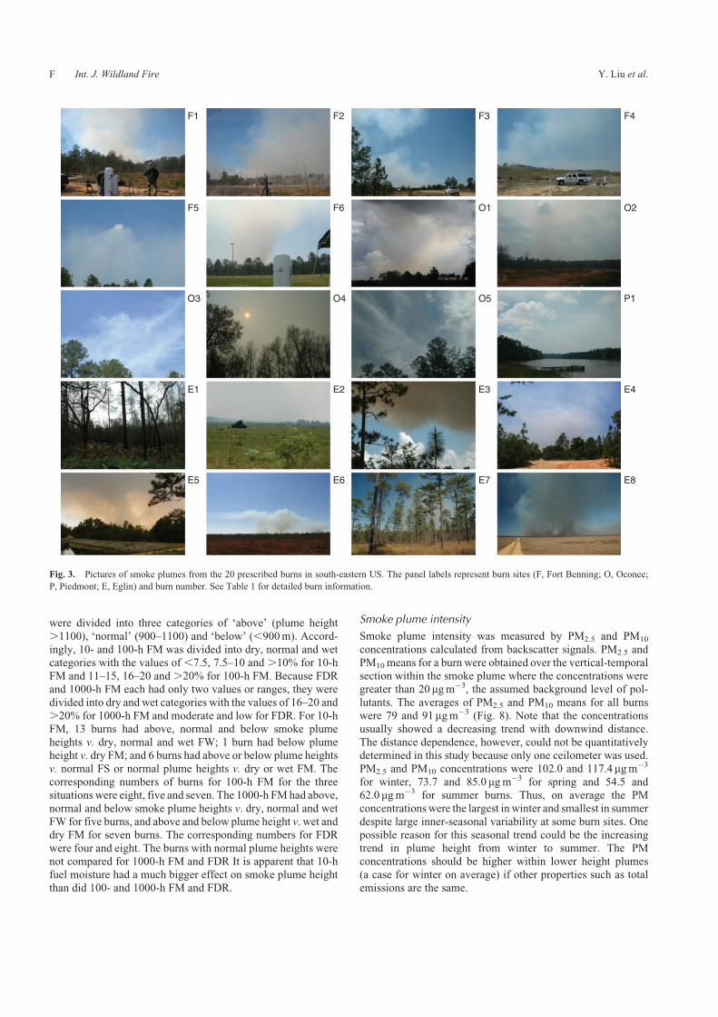
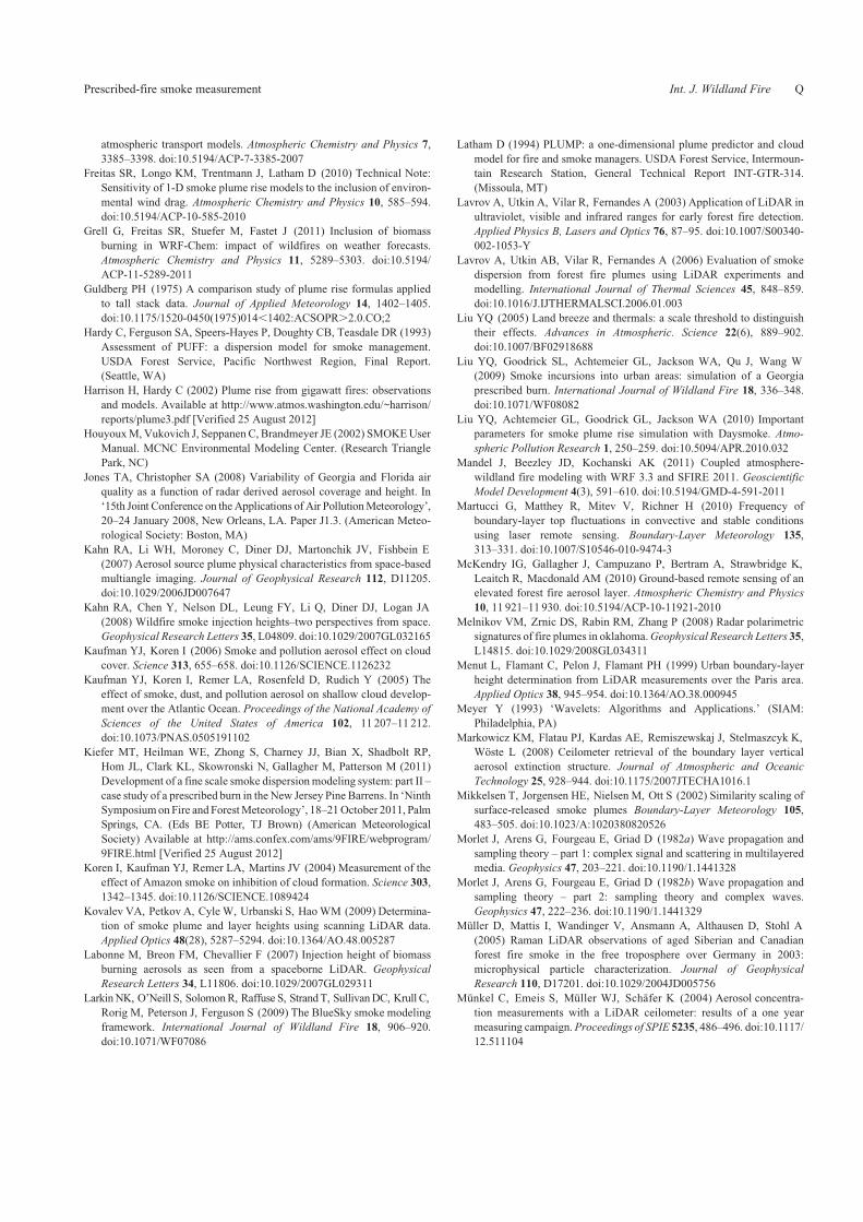
and Piedmont NWR and for five burns at Eglin AFB. Fig. 3shows images of the 20 burns. Smoke plumes were welldeveloped for burns F1, F6, O1, E3–E6 and E8. The sky was

mostly clear for 14 burns, partly cloudy for 3 burns (O4, E3and E4) and mostly cloudy for 3 burns (O1, O2 and P1).

Smoke plume height

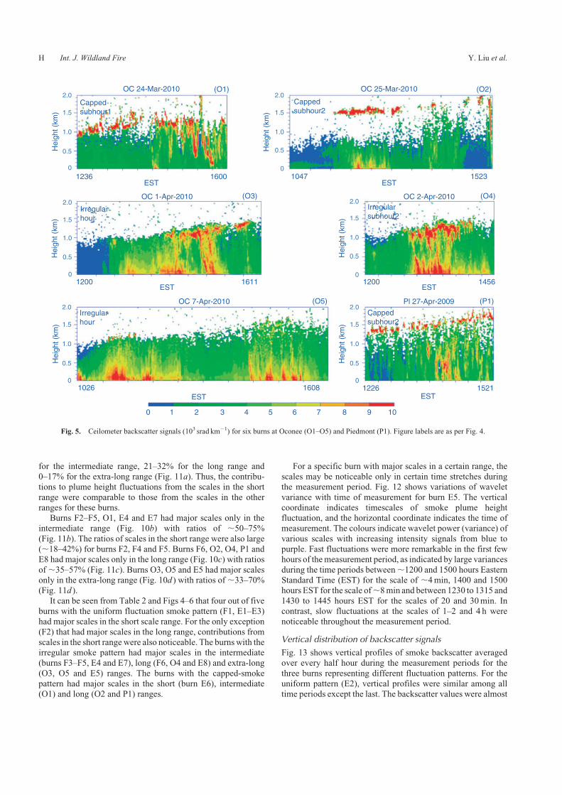
Figs 4–6 show the time-vertical cross-sections of backscatterfrom the prescribed burns. The colours indicate intensity of

backscatter signals, which are proportional to smoke con-centrations. It can be seen that the backscatter signals at a spe-cific time were visible and continuous until a certain elevation,which is the height for smoke plume height, cloud base or the

PBL. Backscatter signals for smoke plumes usually distributedcontinuously within a layer from the ground to the elevation andvaried with time in their intensity. In contrast, backscatter sig-

nals for clouds usually distributed only within a narrow vertical

D Int. J. Wildland Fire Y. Liu et al.

layer around an elevation and maintained mostly constant

intensitywith time. Backscatter signals for the PBLwere usuallyvery weak. For burn O2, for example, weak backscatter signalswere visible within ,500m above ground during the first hour

of the measurement period, whereas slightly more intense sig-nals were visible within ,200m above ground. The elevationsof 500 and 200m were considered as the PBL and smoke plume

heights. Intense signals were seen above 500m after that timeand even more intense signals occurred at ,1500m aboveground, within a layer,100m deep. The elevations of 500 and1500m were considered as smoke plume height and cloud base.

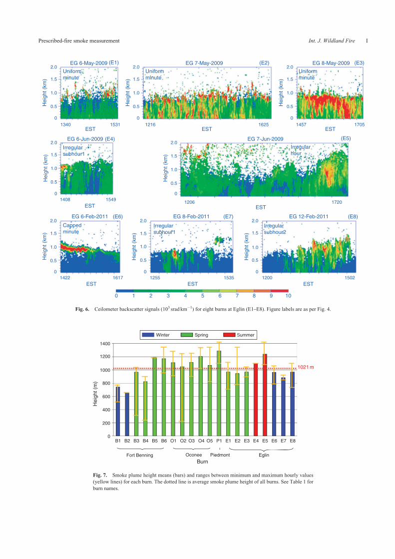
Fig. 7 shows the mean of the smoke plume height over theentire measurement period for each burn. The mean is also listedin Table 2. The average of the smoke plume height means for all

burns was slightly above 1 km. Smoke plume heights variedconsiderably among the burns and depended on the season ofburn occurrence. Smoke plume heights at Fort Benning for the

two burns in mid-January were ,0.75 and 0.65 km; theyincreased to 0.8–0.9 km for the next two burns in early Apriland further increased to nearly 1.2 km for the last twoburns in late

April. Smoke plumeheight is proportional to heat energy releasedfrom fire and atmospheric instability, so burns of larger areaproduce more energy and warmer atmosphere tends to increaseinstability. In this case the last two burns had larger burned areas

and occurred during warmer atmospheric conditions.Smoke plume heights were between ,1.05 and 1.2 km for

the five burns at Oconee NF in late March and early April,

and nearly 1.3 km for the burn at the nearby Piedmont NWR inlate April.

The values at Eglin AFB were between 0.95 and 1 km for the

first three burns in spring; they increased to ,1.1 and 1.25 kmfor the next two burns in early summer and then decreased to,0.9 and ,1 km for the last three burns in late winter.Little difference appeared at this location between the spring

and winter seasons. A possible explanation is that, in spite of

cooler conditions, the burns in early February either had largerburned areas or aerial ignition was used.

The averaged smoke plume height was 842m for the five

winter burns, 1070m for the thirteen spring burns and 1140mfor the two summer burns. Thus, smoke plume height showed anincreasing trend from winter to summer.

Also shown with each mean value in the figure are minimumand maximum hourly values. Hourly values for a specific 1-hperiod (e.g. 1200–1300 local time) were obtained if smokemeasurement during this period was longer than 10min. Smoke

plume height during a burn period can change substantially fromone hour to the next. The difference between minimum andmaximum hourly smoke plume heights was ,300 to 500m for

burns F1, F6, O1, O3–O3, P1, E1, E5–E6 and E8. The largestrange was more than 1000m for burn O2.

Table 3 lists smoke plume height and the corresponding fuel

moisture (FM) and fire-danger rating (FDR) for each burn,obtained from the Remote Automatic Weather Stations (RAWS)(www.raws.fam.nwcg.gov/nfdrs/Weather_station_standards_

rev08_2009_FINAL.pdf, accessed 19 March 2012) and theWildfire Danger Assessment System (WFAS) (www.wfas.net/index.php/fire-danger-rating-fire-potential-danger-32, accessed9 September 2012). The 10-h FM was#7.5% for burns F3–F3,

O3–O5, P1 and E3–E5,.10% for burns F1–F2, E1 and E6–E7,and in between for other burns. The 100-h FM was 11–15% forall but one of the burns (16–20%) at Fort Benning, OconeeNF and

Piedmont NWR, and 16–20% or greater for all burns at EglinAFB. The 1000-h FM was greater than 20% for 16 burns and16–20% for 4 burns. FDRweremostlymoderate at Fort Benning

(five out of six burns) and Oconee NF and Piedmont NWR (fourout of six), and mostly low at Eglin AFB (seven out of eight).

A more detailed analysis of the effects of FM and FDR onplume height was done as follows. Smoke plume height values

Table 1. Prescribed burn information

Burn site Number Name Date Area burned (ha) (acres) Ignition

Fort Benning 1 F1 14-Jan-09 147.3 (364) strip head

2 F2 15-Jan-09 235.9 (583) strip head

3 F3 4-Aug-09 95.5 (236) strip head

4 F4 4-Sep-09 138.8 (343) strip head

5 F5 28-Apr-10 404.7 (1000) strip head

6 F6 29-Apr-10 180.9 (447) strip head

Oconee 7 O1 24-Mar-09 639.4 (1580) aerial

8 O2 25-Mar-10 1011.7 (2500) aerial

9 O3 4-Jan-10 293.4 (725) aerial

10 O4 4-Feb-10 432.6 (1069) aerial

11 O5 4-Jul-10 403.1 (996) aerial

Piedmont 12 P1 27-Apr-09 483.6 (1195) aerial

Eglin 13 E1 5-Jun-09 202.3 (500) strip head

14 E2 5-Jul-09 259.4 (641) strip head

15 E3 5-Aug-09 428.2 (1058) aerial

16 E4 6-Jun-09 607.0 (1500) aerial

17 E5 6-Jul-09 647.5 (1600) aerial

18 E6 2-Jun-11 667.7 (1650) aerial

19 E7 2-Aug-11 828.0 (2046) aerial

20 E8 2-Dec-11 202.3 (500) strip head

Prescribed-fire smoke measurement Int. J. Wildland Fire E

were divided into three categories of ‘above’ (plume height

.1100), ‘normal’ (900–1100) and ‘below’ (,900m). Accord-ingly, 10- and 100-h FM was divided into dry, normal and wetcategories with the values of ,7.5, 7.5–10 and .10% for 10-h

FM and 11–15, 16–20 and .20% for 100-h FM. Because FDRand 1000-h FM each had only two values or ranges, they weredivided into dry and wet categories with the values of 16–20 and

.20% for 1000-h FM and moderate and low for FDR. For 10-hFM, 13 burns had above, normal and below smoke plumeheights v. dry, normal and wet FW; 1 burn had below plumeheight v. dry FM; and 6 burns had above or below plume heights

v. normal FS or normal plume heights v. dry or wet FM. Thecorresponding numbers of burns for 100-h FM for the threesituations were eight, five and seven. The 1000-h FMhad above,

normal and below smoke plume heights v. dry, normal and wetFW for five burns, and above and below plume height v. wet anddry FM for seven burns. The corresponding numbers for FDR

were four and eight. The burns with normal plume heights werenot compared for 1000-h FM and FDR It is apparent that 10-hfuel moisture had a much bigger effect on smoke plume heightthan did 100- and 1000-h FM and FDR.

Smoke plume intensity

Smoke plume intensity was measured by PM2.5 and PM10

concentrations calculated from backscatter signals. PM2.5 andPM10 means for a burn were obtained over the vertical-temporalsection within the smoke plume where the concentrations weregreater than 20 mgm�3, the assumed background level of pol-

lutants. The averages of PM2.5 and PM10 means for all burnswere 79 and 91mgm�3 (Fig. 8). Note that the concentrationsusually showed a decreasing trend with downwind distance.

The distance dependence, however, could not be quantitativelydetermined in this study because only one ceilometer was used.PM2.5 and PM10 concentrations were 102.0 and 117.4mgm�3

for winter, 73.7 and 85.0 mgm�3 for spring and 54.5 and62.0 mgm�3 for summer burns. Thus, on average the PMconcentrationswere the largest inwinter and smallest in summer

despite large inner-seasonal variability at some burn sites. Onepossible reason for this seasonal trend could be the increasingtrend in plume height from winter to summer. The PMconcentrations should be higher within lower height plumes

(a case for winter on average) if other properties such as totalemissions are the same.

F1 F2 F3 F4

F5 F6 O1 O2

O3 O4 O5 P1

E1 E2 E3 E4

E5 E6 E7 E8

Fig. 3. Pictures of smoke plumes from the 20 prescribed burns in south-eastern US. The panel labels represent burn sites (F, Fort Benning; O, Oconee;

P, Piedmont; E, Eglin) and burn number. See Table 1 for detailed burn information.

F Int. J. Wildland Fire Y. Liu et al.

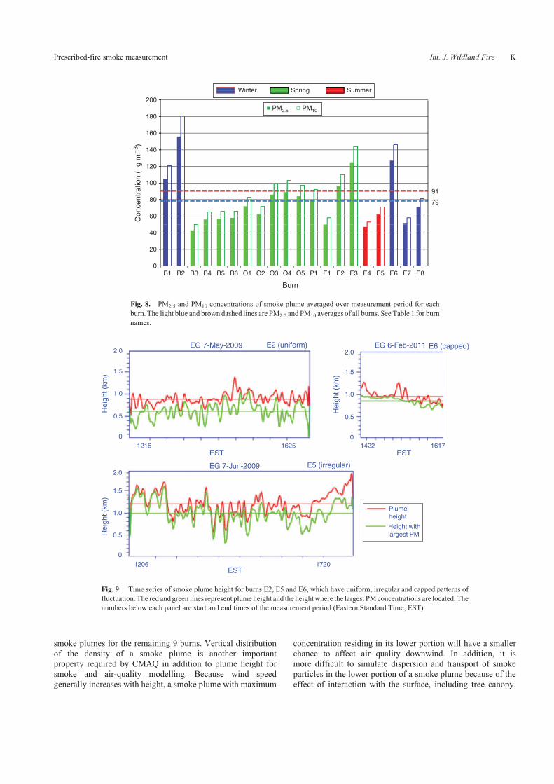
Temporal variability patterns

Smoke plume height and PM concentrations were continuously

dynamic, as shown in Fig. 9. The three burns shown in the figureeach represent a temporal variation pattern. The first pattern(uniform) is characterised by fast and uniform temporal fluc-tuations. Smoke plume height for burn E2 (Fig. 9a) was mostly

within,0.2 km of a height of 0.9 km. Smoke plume heights forburns F1, F2, E1 and E3 also showed the uniform fluctuationpattern.

A second pattern (irregular) was characterised by slow andirregular fluctuations in plume height. Smoke plume height forburn E5 (Fig. 9b) was between,1.2 and 1.7 km in the first hour

of the measurement period, oscillated at,1 km in the following3 h or so, and increased to more than 1.2 km in the final hour.Other plumes with this behaviour were F3–F6, O3–O5, E4, E5,

E7 and E8. Fast fluctuations were superimposed on irregularfluctuations for many burns, especially F4 and F5.

A third pattern (capped) was characterised by a temperatureinversion layer (clear-sky cap) or cloud (cloudy-sky cap) just

above the smoke plumes. Burn E6 (Fig. 9c) was a clear-sky-capcase. As seen in Fig. 3 (E6), the verticallywell-developed smokeplumes drifted horizontally when they reached a certain altitude.

The corresponding smoke plume height gradually decreasedfrom ,1.2 to 0.8 km (Fig. 9c). Burn O1 was a cloudy-sky-capcase, with clouds shown in Fig. 3 (O1). The height of clouds

gradually increased from ,0.9 to 1.3 km during the first 3 h ofthe measurement period; the smoke plume height was,0.8 kmin the first hour and then increased to the cloud height. O2 and P1were two other burns showing the capped pattern. An increasing

or decreasing trend was accompanied by uniform or irregular

fluctuation patterns or both.Variation in the height of the largest PM concentration

followed the variation in smoke plume height for all burns.The distance between the height of largest PMconcentration and

the smoke plume height was mostly constant for the uniformpattern (Fig. 9a). For the irregular fluctuation pattern, thedistance was very small in the first half of the measurement

period but increased in the second half (Fig. 9b). For the cappedpattern the distance was sometimes large during the measure-ment period (Fig. 9c).

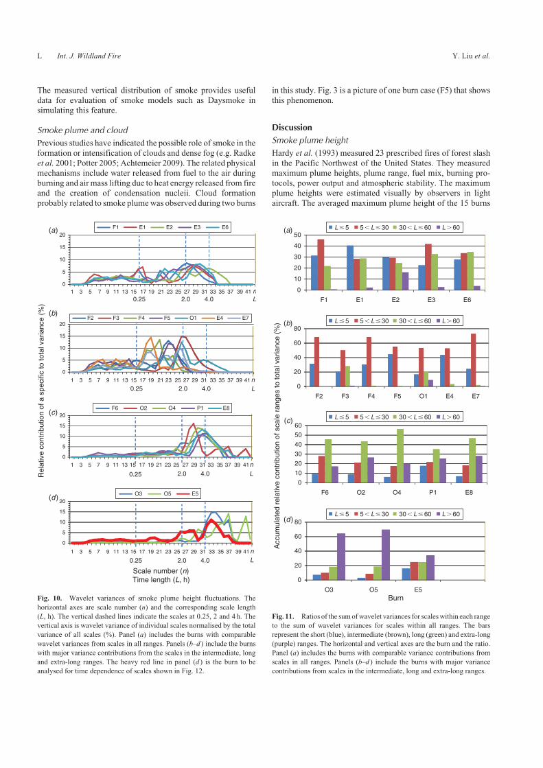
Timescales of fluctuations

Wavelet variances of individual scales in temporal variability ofsmoke plume height are shown in Fig. 10. The values are nor-

malised by the sum of the variances of all scales. The timescalein the wavelet transform measures frequency of fluctuation; theshorter a scale, the faster the fluctuation. Wavelet power (vari-ance) measures intensity of a scale. All scales (t, h) are grouped

into four ranges based on the intensity of themajor scales, whichare defined here as the scales with normalised variances greaterthan 10%: t, 0.25 (short range), 0.25# t, 2 (intermediate),

2# t, 4 (long) and t$ 4 (extra-long).For burns F1, E1–E3 and E6, (Fig. 10a), nomajor scales were

found in the short range or other ranges (in fact, no major scales

were found in the short range for any burn). The ratio of the sumof variances of all scales in a range, to the sum of variances of allscales in all ranges, is shown in Fig. 11. The ratios for these burnswere ,22–40% for the short range, compared with ,28–46%

1235 1250 1312 153513500

0.5

1.0

1.5

2.0

0

0.5

1.0

Hei

ght (

km)

Hei

ght (

km)

Hei

ght (

km)

Hei

ght (

km)

Hei

ght (

km)

Hei

ght (

km)1.5

2.0

0

0.5

1.0

1.5

2.0

0

0.5

1.0

1.5

2.0

0

0.5

1.0

1.5

2.0

0

0.5

1.0

1.5

2.0FB 14-Jan-2009 (F1) (F2) (F3)

(F6)(F5)

(a)

(F4)

FB 15-Jan-2009 FB 8-Apr-2009

1447

1252 1533

0 1 2 3 4 5 6 7 8 9 10

1421 1601

ESTEST EST

ESTEST EST

1109 1340

FB 9-Apr-2009 FB 28-Apr-2010 FB 29-Apr-2010

Uniformminute

Irregularsubhour1

Irregularsubhour1

Irregularsubhour2

Uniformsubhour1

Irregularsubhour1

Fig. 4. Ceilometer backscatter signals (103 srad km�1) for six burns at Fort Benning (F1–F6). The two numbers below each panel are start and end times

(Eastern Standard Time, EST) of the smoke measurement period. The backscatter intensity (equivalent to PM concentrations) is indicated by the colours. The

burn site and date are shown on top of each panel. Descriptors of the fluctuation pattern and major scale range are given within each panel.

Prescribed-fire smoke measurement Int. J. Wildland Fire G

for the intermediate range, 21–32% for the long range and0–17% for the extra-long range (Fig. 11a). Thus, the contribu-tions to plume height fluctuations from the scales in the short

range were comparable to those from the scales in the otherranges for these burns.

Burns F2–F5, O1, E4 and E7 had major scales only in theintermediate range (Fig. 10b) with ratios of ,50–75%

(Fig. 11b). The ratios of scales in the short range were also large(,18–42%) for burns F2, F4 and F5. Burns F6, O2, O4, P1 andE8 had major scales only in the long range (Fig. 10c) with ratios

of,35–57% (Fig. 11c). Burns O3, O5 and E5 had major scalesonly in the extra-long range (Fig. 10d ) with ratios of,33–70%(Fig. 11d ).

It can be seen from Table 2 and Figs 4–6 that four out of fiveburns with the uniform fluctuation smoke pattern (F1, E1–E3)had major scales in the short scale range. For the only exception

(F2) that had major scales in the long range, contributions fromscales in the short rangewere also noticeable. The burns with theirregular smoke pattern had major scales in the intermediate(burns F3–F5, E4 and E7), long (F6, O4 and E8) and extra-long

(O3, O5 and E5) ranges. The burns with the capped-smokepattern had major scales in the short (burn E6), intermediate(O1) and long (O2 and P1) ranges.

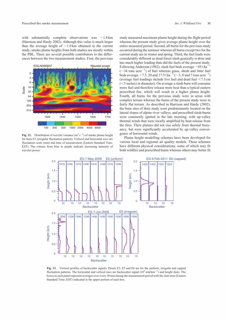
For a specific burn with major scales in a certain range, thescales may be noticeable only in certain time stretches duringthe measurement period. Fig. 12 shows variations of wavelet

variance with time of measurement for burn E5. The verticalcoordinate indicates timescales of smoke plume heightfluctuation, and the horizontal coordinate indicates the time ofmeasurement. The colours indicate wavelet power (variance) of

various scales with increasing intensity signals from blue topurple. Fast fluctuations were more remarkable in the first fewhours of themeasurement period, as indicated by large variances

during the time periods between,1200 and 1500 hours EasternStandard Time (EST) for the scale of ,4min, 1400 and 1500hours EST for the scale of,8min and between 1230 to 1315 and

1430 to 1445 hours EST for the scales of 20 and 30min. Incontrast, slow fluctuations at the scales of 1–2 and 4 h werenoticeable throughout the measurement period.

Vertical distribution of backscatter signals

Fig. 13 shows vertical profiles of smoke backscatter averagedover every half hour during the measurement periods for the

three burns representing different fluctuation patterns. For theuniform pattern (E2), vertical profiles were similar among alltime periods except the last. The backscatter values were almost

2.0

1.5

1.0

0.5

0

2.0

1.5

1.0

0.5

0

2.0

1.5

1.0

0.5

0

(O3)

(O1) (O2)

(O4)

(O5) (P1)

Hei

ght (

km)

Hei

ght (

km)

Hei

ght (

km)

Hei

ght (

km)

Hei

ght (

km)

Hei

ght (

km)

2.0

1.5

1.0

0.5

0

2.0

1.5

1.0

0.5

0

Cappedsubhour1

Cappedsubhour2

Irregularhour

Irregularhour

Irregularsubhour2

Cappedsubhour2

1047 1523

1200 1611 1200 1456

1226EST

EST

15211026

0 1 2 3 4 5 6 7 8 9 10

EST

EST

ESTEST

1608

2.0

1.5

1.0

0.5

0

1236 1600

OC 24-Mar-2010 OC 25-Mar-2010

OC 2-Apr-2010

Pl 27-Apr-2009

OC 1-Apr-2010

OC 7-Apr-2010

Fig. 5. Ceilometer backscatter signals (103 srad km�1) for six burns at Oconee (O1–O5) and Piedmont (P1). Figure labels are as per Fig. 4.

H Int. J. Wildland Fire Y. Liu et al.

)3E()2E((E1)

Uniformminute

Uniformminute

Uniformminute

(E4) (E5)

(E6) (E7) (E8)

Irregularhour

Irregularsubhour2

Irregularsubhour1

Irregularsubhour1

Cappedminute

2.0

1.5

1.0

0.5

0

2.0

1.5

1.0

0.5

0

2.0

1.5

1.0

0.5

0

2.0

1.5

1.0

0.5

0

Hei

ght (

km)

Hei

ght (

km)

Hei

ght (

km)

Hei

ght (

km)

Hei

ght (

km)

2.0

1.5

1.0

0.5

0

Hei

ght (

km)

1340 1531

EST

EST EST EST

1408 1549

2.0

1.5

1.0

0.5

0

2.0

1.5

1.0

0.5

0

Hei

ght (

km)

EST ESTEST1422 1617 1255

0 1 2 3 4 5 6 7 8 9 10

1535

2.0

1.5

1.0

0.5

0

Hei

ght (

km)

1200 1502

EST1206 1720

1216 1625 1457 1705

EG 6-May-2009

EG 6-Jun-2009 EG 7-Jun-2009

EG 7-May-2009 EG 8-May-2009

EG 6-Feb-2011 EG 8-Feb-2011 EG 12-Feb-2011

Fig. 6. Ceilometer backscatter signals (103 srad km�1) for eight burns at Eglin (E1–E8). Figure labels are as per Fig. 4.

1021 m

Hei

ght (

m)

B10

200

400

600

800

1000

1200

1400

B2 B3 B4 B5 B6 O1 O2 O3 O4 O5 P1 E1 E2 E3 E4 E5 E6 E7 E8

BurnFort Benning Oconee Piedmont Eglin

SummerSpringWinter

Fig. 7. Smoke plume height means (bars) and ranges between minimum and maximum hourly values

(yellow lines) for each burn. The dotted line is average smoke plume height of all burns. See Table 1 for

burn names.

Prescribed-fire smoke measurement Int. J. Wildland Fire I

constant from the ground to a certain height where they gradu-ally decreased towards the top of the smoke plume. Backscatterat a height of 0.8 km is very large during the last time period.

This wasmost likely related to a new and intense ignition duringthe strip lighting process, although a definitive explanationcannot be provided without knowledge of the actual ignitiontime and fire intensity. For the irregular pattern (E5), large

backscatter signals first occured in the lower portion of thesmoke plume, but later moved to the upper portion. For thecapped pattern (E6), large backscatter signals were found near

the top of the smoke plume.Among the 20 burns, large backscatter signals occurred

mostly in the upper portion of smoke plumes for 8 burns, andthe lower, for 3 burns, but did not change much vertically within

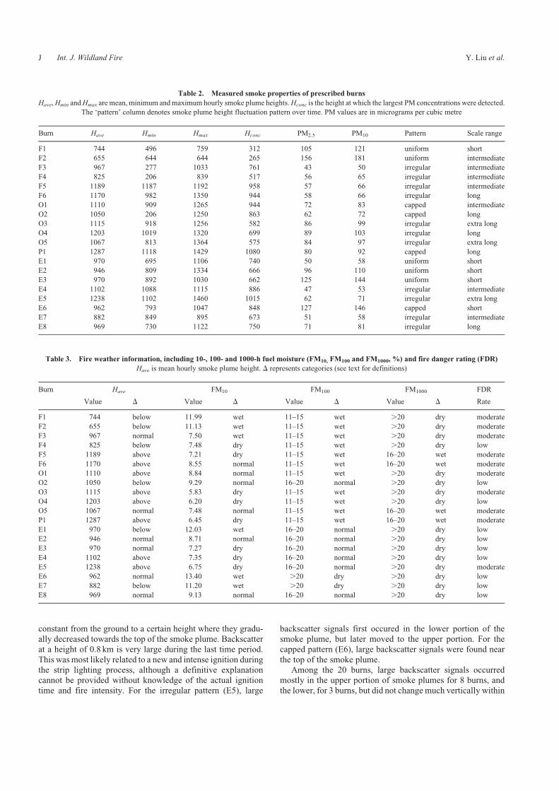
Table 2. Measured smoke properties of prescribed burns

Have,Hmin andHmax are mean, minimum andmaximum hourly smoke plume heights.Hconc is the height at which the largest PM concentrations were detected.

The ‘pattern’ column denotes smoke plume height fluctuation pattern over time. PM values are in micrograms per cubic metre

Burn Have Hmin Hmax Hconc PM2.5 PM10 Pattern Scale range

F1 744 496 759 312 105 121 uniform short

F2 655 644 644 265 156 181 uniform intermediate

F3 967 277 1033 761 43 50 irregular intermediate

F4 825 206 839 517 56 65 irregular intermediate

F5 1189 1187 1192 958 57 66 irregular intermediate

F6 1170 982 1350 944 58 66 irregular long

O1 1110 909 1265 944 72 83 capped intermediate

O2 1050 206 1250 863 62 72 capped long

O3 1115 918 1256 582 86 99 irregular extra long

O4 1203 1019 1320 699 89 103 irregular long

O5 1067 813 1364 575 84 97 irregular extra long

P1 1287 1118 1429 1080 80 92 capped long

E1 970 695 1106 740 50 58 uniform short

E2 946 809 1334 666 96 110 uniform short

E3 970 892 1030 662 125 144 uniform short

E4 1102 1088 1115 886 47 53 irregular intermediate

E5 1238 1102 1460 1015 62 71 irregular extra long

E6 962 793 1047 848 127 146 capped short

E7 882 849 895 673 51 58 irregular intermediate

E8 969 730 1122 750 71 81 irregular long

Table 3. Fire weather information, including 10-, 100- and 1000-h fuel moisture (FM10, FM100 and FM1000, %) and fire danger rating (FDR)

Have is mean hourly smoke plume height. D represents categories (see text for definitions)

Burn Have FM10 FM100 FM1000 FDR

Value D Value D Value D Value D Rate

F1 744 below 11.99 wet 11–15 wet .20 dry moderate

F2 655 below 11.13 wet 11–15 wet .20 dry moderate

F3 967 normal 7.50 wet 11–15 wet .20 dry moderate

F4 825 below 7.48 dry 11–15 wet .20 dry low

F5 1189 above 7.21 dry 11–15 wet 16–20 wet moderate

F6 1170 above 8.55 normal 11–15 wet 16–20 wet moderate

O1 1110 above 8.84 normal 11–15 wet .20 dry moderate

O2 1050 below 9.29 normal 16–20 normal .20 dry low

O3 1115 above 5.83 dry 11–15 wet .20 dry moderate

O4 1203 above 6.20 dry 11–15 wet .20 dry low

O5 1067 normal 7.48 normal 11–15 wet 16–20 wet moderate

P1 1287 above 6.45 dry 11–15 wet 16–20 wet moderate

E1 970 below 12.03 wet 16–20 normal .20 dry low

E2 946 normal 8.71 normal 16–20 normal .20 dry low

E3 970 normal 7.27 dry 16–20 normal .20 dry low

E4 1102 above 7.35 dry 16–20 normal .20 dry low

E5 1238 above 6.75 dry 16–20 normal .20 dry moderate

E6 962 normal 13.40 wet .20 dry .20 dry low

E7 882 below 11.20 wet .20 dry .20 dry low

E8 969 normal 9.13 normal 16–20 normal .20 dry low

J Int. J. Wildland Fire Y. Liu et al.

smoke plumes for the remaining 9 burns. Vertical distributionof the density of a smoke plume is another important

property required by CMAQ in addition to plume height forsmoke and air-quality modelling. Because wind speedgenerally increases with height, a smoke plume with maximum

concentration residing in its lower portion will have a smallerchance to affect air quality downwind. In addition, it is

more difficult to simulate dispersion and transport of smokeparticles in the lower portion of a smoke plume because of theeffect of interaction with the surface, including tree canopy.

180

200

140

160

100

120

91

60

80 79

20

40

Con

cent

ratio

n (µ

g m

�3 )

0B1 B2 B3 B4 B5 B6 O1 O2 O3 O4 O5 P1 E1 E2 E3 E4 E5 E6 E7 E8

Burn

Winter Spring Summer

PM2.5 PM10

Fig. 8. PM2.5 and PM10 concentrations of smoke plume averaged over measurement period for each

burn. The light blue and brown dashed lines are PM2.5 and PM10 averages of all burns. See Table 1 for burn

names.

E2 (uniform) E6 (capped)

E5 (irregular)

Plumeheight

Height withlargest PM

1216EST EST

EG 7-May-2009

EG 7-Jun-2009

EG 6-Feb-2011

Hei

ght (

km)

2.0

1.5

1.0

0.5

0

Hei

ght (

km)

2.0

1.5

1.0

0.5

0

Hei

ght (

km)

2.0

1.5

1.0

0.5

0

1625 1422 1617

1206EST

1720

Fig. 9. Time series of smoke plume height for burns E2, E5 and E6, which have uniform, irregular and capped patterns of

fluctuation. The red and green lines represent plume height and the heightwhere the largest PMconcentrations are located. The

numbers below each panel are start and end times of the measurement period (Eastern Standard Time, EST).

Prescribed-fire smoke measurement Int. J. Wildland Fire K

The measured vertical distribution of smoke provides usefuldata for evaluation of smoke models such as Daysmoke insimulating this feature.

Smoke plume and cloud

Previous studies have indicated the possible role of smoke in theformation or intensification of clouds and dense fog (e.g. Radke

et al. 2001; Potter 2005; Achtemeier 2009). The related physicalmechanisms include water released from fuel to the air duringburning and air mass lifting due to heat energy released from fire

and the creation of condensation nucleii. Cloud formationprobably related to smoke plumewas observed during two burns

in this study. Fig. 3 is a picture of one burn case (F5) that showsthis phenomenon.

Discussion

Smoke plume height

Hardy et al. (1993) measured 23 prescribed fires of forest slash

in the Pacific Northwest of the United States. They measuredmaximum plume heights, plume range, fuel mix, burning pro-tocols, power output and atmospheric stability. The maximum

plume heights were estimated visually by observers in lightaircraft. The averaged maximum plume height of the 15 burns

10

15

20

F2 F3 F4 F5 O1 E4 E7

0

5

0.25 2.0 4.0 Ln

5

10

15

20

F6 O2 O4 P1 E8

0

0.25 2.0 4.0

5

10

15

20

0

20O3 O5 E5

0

5

10

15

Rel

ativ

e co

ntrib

utio

n of

a s

peci

fic to

tota

l var

ianc

e (%

)

1 3 5 7 9 11 13 15 17 19 21 23 25 27 29 31 33 35 37 39 41

L1 3 5 7 9 11 13 15 17 19 21 23 25 27 29 31 33 35 37 39 41 n

L1 3 5 7 9 11 13 15 17 19 21 23 25 27 29 31 33 35 37 39 41 n

0.25 2.0 4.0

L1 3 5 7 9 11 13 15 17 19 21 23 25 27 29 31 33 35 37 39 41 n

0.25 2.0 4.0

Scale number (n)Time length (L, h)

F1 E1 E2 E3 E6(a)

(b)

(c)

(d )

Fig. 10. Wavelet variances of smoke plume height fluctuations. The

horizontal axes are scale number (n) and the corresponding scale length

(L, h). The vertical dashed lines indicate the scales at 0.25, 2 and 4 h. The

vertical axis is wavelet variance of individual scales normalised by the total

variance of all scales (%). Panel (a) includes the burns with comparable

wavelet variances from scales in all ranges. Panels (b–d ) include the burns

with major variance contributions from the scales in the intermediate, long

and extra-long ranges. The heavy red line in panel (d ) is the burn to be

analysed for time dependence of scales shown in Fig. 12.

(a)

20

30

40

50

(b)

0

10

40

60

80

(c)

0

20

30

40

50

60

(d )

0

10

20

40

60

80

Burn

0

20

F1 E1 E2 E3 E6

F2 F3 F4 F5 O1 E4 E7

F6 O2 O4 P1 E8

O3 O5 E5

L � 5 5 � L � 30 30 � L � 60 L � 60

L � 5 5 � L � 30 30 � L � 60 L � 60

L � 5 5 � L � 30 30 � L � 60 L � 60

L � 5 5 � L � 30 30 � L � 60 L � 60

Acc

umul

ated

rel

ativ

e co

ntrib

utio

n of

sca

le r

ange

s to

tota

l var

ianc

e (%

)

Fig. 11. Ratios of the sumofwavelet variances for scaleswithin each range

to the sum of wavelet variances for scales within all ranges. The bars

represent the short (blue), intermediate (brown), long (green) and extra-long

(purple) ranges. The horizontal and vertical axes are the burn and the ratio.

Panel (a) includes the burns with comparable variance contributions from

scales in all ranges. Panels (b–d ) include the burns with major variance

contributions from scales in the intermediate, long and extra-long ranges.

L Int. J. Wildland Fire Y. Liu et al.

with substantially complete observations was ,1.8 km(Harrison and Hardy 2002). Although this value is much largerthan the average height of ,1.0 km obtained in the current

study, smoke plume heights from both studies are mostly withinthe PBL. There are several possible contributors to the differ-ences between the two measurement studies. First, the previous

study measured maximum plume height during the flight periodwhereas the present study gives average plume height over theentire measured period. Second, all burns for the previous study

occurred during the summerwhereas all burns except two for thecurrent study are in winter and spring. Third, the fuel loads wereconsiderably different as dead forest slash generally is drier and

has much higher loading than did the fuels of the present study.Following Anderson (1982), slash fuel beds average,85 t ha�1

(,34 tons acre�1) of fuel whereas grass, shrub and litter fuel

beds average,7.5, 20 and 17.5 t ha�1 (,3, 8 and 7 tons acre�1)(average fuel loadings include live fuel and dead fuel ,7.5 cm(,3 inches) in diameter). On average a slash burn will consumemore fuel and therefore release more heat than a typical eastern

prescribed fire, which will result in a higher plume height.Fourth, all burns for the previous study were in areas withcomplex terrain whereas the burns of the present study were in

fairly flat terrain. As described in Harrison and Hardy (2002),the burn sites of their study were predominantly located on thelateral slopes of alpine river valleys, and prescribed slash-burns

were commonly ignited in the late morning, with up-valleythermal winds that were locally amplified by heat release fromthe fires. Their plumes did not rise solely from thermal buoy-

ancy, but were significantly accelerated by up-valley conver-gence of horizontal winds.

Plume height modelling schemes have been developed forvarious local and regional air quality models. These schemes

have different physical considerations, some of which may fitboth wildfire and prescribed burns whereas others may better fit

1300

Sca

le

512

252

128

64

32

16

8

4

2

100 200 500 1000 2000 4000 8000

1400 1500 1600 1700

EGLN090607 Wavelet power

Fig. 12. Distribution of wavelet variance (m2 s�2) of smoke plume height

for burn E5 (irregular fluctuation pattern). Vertical and horizontal axes are

fluctuation scale (min) and time of measurement (Eastern Standard Time,

EST). The colours from blue to purple indicate increasing intensity of

wavelet power.

E2 (uniformEG 7-May-2009 EG 6-Feb-2011

EG 7-Jun-2009

) E6 (capped)

1216 1246 1316

100

0.5

1.0

1.5

2.0

0

0.5

1.0

1.5

2.0

0

0.5

Hei

ght (

km)

Hei

ght (

km)

Hei

ght (

km)

1.0

1.5

2.0

10 10 10 10 10 10 10 10 10 10 10

1346 1416 1446 1516 1546 1422 1452 1522 1552

E5 (irregular)

1206 1236 1306 1336 1406 1436 1506 1536 1606 1636

10 10 10 101010 10 10 10 10

Backscatter

Backscatter Backscatter

Fig. 13. Vertical profiles of backscatter signals. Panels E2, E5 and E6 are for the uniform, irregular and capped

fluctuation patterns. The horizontal and vertical axes are backscatter signal (103 srad km�1) and height (km). The

boxes in each panel represent averages over every 30min during the measurement period with the start time (Eastern

Standard Time, EST) indicated in the upper portion of each box.

Prescribed-fire smoke measurement Int. J. Wildland Fire M

just one of these. Understanding the strengths andweaknesses ofvarious schemes in modelling prescribed burn plume height canbe improved through inter-comparing these schemes using the

measured data from this study. Trentmann et al. (2002) usedairborne remote sensing and in situ smoke plume measurementsto compare the simulated dynamic evolution of a plume from a

prescribed fire with the active tracer high-resolution atmosphericmodel. Previous investigations like Trentmann et al. (2002)have largely focussed on one burn or a very limited number of

prescribed burns. The present study, however, measured a largenumber of burns; thus, the results can be used as systematicand statistical evaluation data for prescribed-burn modelperformance.

The measurements could be used to evaluate the capacity ofsmoke models in simulating the plume features observed in thisstudy, including fluctuations at different timescales, and differ-

ent types of vertical profiles and particulate matter concentra-tions. The fluctuation and varied vertical distribution featuresare related to fuels and ecosystem types, fire emissions and heat-

energy release, atmospheric turbulence and eddy motions, andother complex dynamic and thermal processes. Thus, it isdifficult for smoke models to reproduce these features. Evalua-

tions would provide useful information to improve the descrip-tion of these processes in smoke models. Unfortunately nometeorological data (profiles or surface values of wind speedand direction, temperature and turbulence) were collected

during this study. These data are key determinants in plume riseand inputs in plume height models. Therefore the use of thisdataset for the evaluation of plume height models for these types

of buoyant sources is limited.The measured smoke plume height could also be used to help

estimate smoke plume parameters such as updraft core number

(used in Daysmoke). Multiple updraft cores are smoke ‘sub-plumes’ and are the outcome ofmultiple ignitions, smoke plumeinteractions, heterogeneous distributions of fuels and otherprocesses. Sub-plumes may initially rise separately and later

merge into a single plume. The buoyancy created by multipleupdraft cores is smaller than that generated by one single updraftcore with a size equivalent to the integrated size of all updraft

cores. The corresponding plume height is therefore smaller. Thecore number is one of the most important parameters in Day-smoke for plume height calculation (Liu et al. 2010; Achtemeier

et al. 2011). However, this parameter is typically unavailable.Detection techniques and calculation schemes are yet to bedeveloped. Achtemeier et al. (2011) found that Daysmoke obeys

the 2/3 law for plume rise, similar to the Briggs plume risescheme (Briggs 1975), for most plumes. The factors in smokeplume rise include heat flux, wind speed and entrainmentcoefficient; heat flux is determined by updraft core number,

exit temperature and velocity, and burned area. Using the plumeheightmeasurements from this study, updraft core number couldbe retrieved if other parameters are known. However, this work

is beyond this study because measurements and modelling offuel, fire behaviour, and meteorology are needed to obtain theseparameters.

Temporal variability of smoke plume height

Many studies of individual prescribed burns have found timefluctuations with smoke plumes. For example, Lavrov et al.

(2006) scanned a smoke plume from an experimental prescribedburn of,1.01 ha (,2.5 acres) with a LiDAR and found doublepeaks in horizontal distribution of smoke particle concentra-

tions. Simulations with a Reynolds-averaged Navier–Stokesfluid dynamical model showed fluctuations with time. Thepresent study provides detailed features of fluctuations for

multiple prescribed burns. The new finding indicates that thetemporal smoke fluctuations include fast and uniform fluctua-tions at the time scales of minutes for almost all burns and slow

and irregular fluctuations at the scales of tens ofminutes to hoursfor some burns.

Martucci et al. (2010) found that the salient frequency ofdaytime thermal updrafts and downdrafts averaged over five

cases was 2.6mHz (equivalent to a time scale of 6.5min). Thissuggests that the fluctuations of thermal processes in the PBLcould be one of the causes for the fast and uniform fluctuations in

the smoke plume observed in this study. The fluctuations insmoke plume height at longer scales could be related to acombination of the ignition times and methods, amount of fuel

that is available (dry enough) to burn at thatmoment, the amountof fuel contained in the ecosystem, antecedent and current fireweather (i.e. humidity, wind, temperature) and atmospheric

processes. Fire ignition is often conducted intermittently.Consequently, smoke particles can enter the atmosphere as aseries of puffs or cells and buoyancy can change due to temporalchanges in burn behaviour. Small-scale turbulence, variations in

wind direction and speed, changes in vertical stability andchanges in the internal boundary layer due to surface roughnessalso contribute to particulate-mass fluctuations within the

smoke plume. In a PBL without strong winds, the smoke plumecan be well organised and rise vertically with strong buoyancygenerated from heat energy released during burning. The plume

stops rising when encountering a strong inversion, reachingtemperature equilibrium with the surrounding atmosphere, orentraining enough ambient air (through wind and turbulentmixing) so that it loses its initial buoyancy.

The scales of smoke plume height fluctuations show depen-dence on time, that is, certain scales may be remarkable only atsome times of the burning period. Fuels are often heterogeneous

within a burned area and the fuels to be burned can be different atvarious burning stages. So are the atmospheric conditions. Thedifferences may be responsible for the time dependence of

scales. This feature is useful for understanding the effects offuel, fire behaviour and atmospheric processes on smokedynamics. If temporal variations of fire behaviour and atmo-

spheric conditions are known, it would be possible to understandthe mechanisms for the fluctuations from the variations.

The effect of canopy is another important factor that needs tobe included in smoke plume models. Vegetation can affect

turbulence, buoyancy and heat transfer within smoke near theground and therefore, dispersion and transport of smoke. Thisrole has been examined recently in, for example, Kiefer et al.

(2011). A canopy sub-model was developed for a regionalatmospheric prediction system and used to simulate the effectsof forest vegetation on the atmospheric boundary-layer dynam-

ics and the smoke plume from a prescribed fire. The groundtower measurements indicated fast fluctuations in the meteoro-logical fields. Given the complex mechanisms for the fluctua-tions within smoke plumes, smoke plume models will need to

N Int. J. Wildland Fire Y. Liu et al.

describe multiple processes or effects of fuel, ignition, canopy,turbulence and atmospheric thermodynamics. The smoke mea-surements from this study could provide additional information

for evaluating simulation of vegetation–atmosphere–smokeinteractions. The fast and irregular fluctuations in smoke plumeheight affect both small-scale modelling of specific plumes and

large-scale chemical transport modelling. The type of LiDARdata provided here can serve to both improve currentmodels andto verify modelled results.

Satellite remote sensing has emerged as a useful technique todetect and monitor wildland fires and smoke. There has beenlimited exploration of the potential for satellite data to detectsmall and cool burning fires (e.g. Wang et al. 2007). Nonethe-

less, in comparison to wildfires, prescribed fires are typicallysmaller in terms of area burned, fireline length, and fire intensityand life time, all of which inhibit the ability of satellite instru-

ments to detect them. Additionally, prescribed burning is oftenin the understorey vegetation, which further hampers detectionfrom space. Satellite instruments are not currently able to

detect smoke fluctuations or to consistently view smoke plumedevelopment and dynamics. Satellite data such as ModerateResolution Imaging Spectroradiometer (MODIS), CALIOP,

Geostationary Operational Environmental Satellites (GOES)and MISR are often able to capture smoke plumes duringoverhead passes within the resolution of the instruments. Smokeplume injection height can be identified with MISR (morning

only overpass) and CALIOP (low temporal frequency andhorizontal resolution) data. MISR and CALIOP are both globalproducts and could provide the statistics necessary to calculate

maximum, mean and minimum plume heights within large-scale ecosystems. AMISRproduct is available (ValMartin et al.2010) and a CALIOP plume height product is under development

(http://misr.jpl.nasa.gov/getData/accessData/MisrMinxPlumes/,accessed 9 September 2012). Thus, even though satellite datacould provide statistics, they are not complete for detailedmodelling of plume evolution and dynamics.

Vertical structure

The vertical profile of smoke plume mass is another property in

addition to plume rise that is required by regional air qualitymodels such as CMAQ. The vertical profiles measured in thisstudy are expected to be useful for evaluating smoke dynamics

modelling with smoke models such as Daysmoke. The verticalprofiles averaged over the ceilometer measurement period showthat approximately half of the 20 burns had more intense

backscatter signals and therefore larger PM concentrations inthe lower portion of the smoke plume nearer the ground than inthe upper portion of the smoke plume. However, occurrences ofdenser smoke on the ground or in the lower portion of the smoke

plume were observed by the measurement crew only for a fewburns and mostly only for brief periods during the measure-ments. This suggests that the ceilometer might overestimate

smoke density in the lower portion of smoke plumes while over-attenuating smoke signals in the upper portion. Tsai et al. (2009)indicated that backscatter signals from a CL31 ceilometer were

more intense than those from a radar in the lower portion of asmoke plume, but were strongly attenuated above 1 km. Theceilometer backscatter signal intensity is determined by threeheight-dependent factors: extinction coefficient of atmospheric

particles, backscatter coefficient and height normalisation(inversely proportional to the square of the height in a clearatmosphere) (Vaisala, see www.vaisala.com, accessed 26

August 2012). More calibrations of these parameters for smokeparticles are needed. Note that, despite the possible over-excessive attenuation in the upper portion of a smoke plume, the

ceilometer received a sufficient amount of backscatter at the topof the plume for determining height.

The enhanced optics and electronics of the CL31 ceilometer

enable it to detect boundary-layer height with high resolution(Munkel et al. 2007). Several methods for retrieving mixing-layer height from LiDAR backscatter profiles have been pre-sented (Menut et al. 1999; Steyn et al. 1999; Cohn andAngevine

2000; Davis et al. 2000), and are based on a sudden change ineither backscatter or its gradient at the top of the mixing layer.Similar variations were seen in the present study at certain times

during the measurement period for some burns (e.g. Fig. 4(F3–F5), Fig. 5 (O2–O3) and Fig. 6 (E7–E8)). However, it isdifficult to identify the PBL height for many other burn cases.

All the burns were conducted in rural areas or near small townswhere the background pollutants were much less dense thanthose in urban areas. In addition, most burns happened in the

afternoon when the PBL during this time of year was likely to becollapsing and the background pollutants might be hard toseparate from the smoke particles.

Smoke and clouds

This study recorded two cases where clouds seemed to havedeveloped during vertical expansion and upward movement ofthe smoke plume. This provides new evidence for a possible role

of smoke in atmospheric moist processes such as clouds anddense fog, as suggested by previous studies. Radke et al. (2001)proposed using clouds as part of the prescription for scheduling

biomass fires because clouds and precipitation are the principalmechanisms by which the atmosphere is cleansed of particulatepollution, aerosols and smoke. The observed clouds in this

study, however, appeared without producing precipitation. Inthis case, the smoke-generated clouds from those prescribedburns affected smoke dispersion and transport processes, butthey were not developed enough to precipitate and remove

smoke particles from the atmosphere. There have been numer-ous studies to date that suggest biomass burning can influenceand potentially alter patterns of rainfall (not necessarily act as

cloud concentration nuclei to stimulate rainfall). Uncertaintiesin the relationship between smoke, precipitation and cloud coverhave also been highlighted (Andreae et al. 2004; Koren et al.

2004; Kaufman et al. 2005; Kaufman and Koren 2006).

Conclusions

Measurements and analyses have been taken for 20 prescribedburns in the south-eastern US using a ceilometer. The average

plume height was ,1 km. When models or measurements arenot available, fire managers could use the results as an empiricalguideline to estimate smoke plume height in the south-eastern

US. The average height could be used as a first-order approxi-mation for smoke plume height for prescribed burns in thisregion. A second-order approximation could be used by makingseasonal adjustment for this region based on the increasing trend

Prescribed-fire smoke measurement Int. J. Wildland Fire O

of smoke plume heights from winter to summer. Higher-orderapproximations could be obtained by further makingadjustments by considering hours of the day, cloud height,

temperature, background wind and other fuel and fire weathervariables. This approach is similar to the one used in developingtheWesternRegional Air Partnership (2005) plume rise scheme.

Of course, actual plume height shows large variability betweenand within burns, even for those in the same season andecosystem. Smoke plume models are needed to estimate more

accurate plume height of a specific burn, and data from thisstudy can be used both to verify and refine models.

Smoke particle concentrations near the burn sites are large inthe PBL. The average PM2.5 and PM10 concentrations within

smoke plumes calculated based on the ceilometer backscattersignals are,80 and 90mgm�3. On average the PM2.5 and PM10

concentrations decrease from winter to summer. This seasonal

trendmay be related to the increasing trend in plume height fromwinter to summer. Further research is needed to understand theroles of fuel property, burn technique and atmospheric

conditions.Almost all burns show fast and uniform fluctuations at

minute scales. A substantial number of burns also show slow

and irregular fluctuations at scales from tens ofminutes to hours,which increases the degree of difficulty in detecting prescribed-burn smoke using satellite data because the detected smokeplume height may vary considerably from one time to another.

Fluctuations are influenced by complex burn and atmosphericprocesses. Further research is needed to understand the detailedconnections.

The smoke plumes have varied vertical profiles. Largebackscatter signals are found in the lower portion of smokeplumes for many burns. More inter-comparison studies with

different detection techniques will help understand if this isa realistic feature of smoke plumes or is caused by under-attenuation of smoke signals at lower elevations with ceilometerdetection, as found in a previous study.

The measured smoke plume height data will be used toevaluate Daysmoke. They will also be used to formulate asemi-empirical scheme to estimate smoke plume height, as

was done by Harrison and Hardy (2002). The relationshipsbetween the measured smoke plume heights and fuel andatmospheric conditions (temperature, moisture, winds, etc.) will

be established using statistical and similarity analysistechniques. These conditions are available to fire managers.Such schemes therefore should be practically useful for fire

managers to estimate smoke plume height of prescribed burns,which will provide important information for further estimatingsmoke dispersion and transport to remote areas. Such schemescould also be used to assess smoke-air-quality effect simulations

with regional air-quality models such as CMAQ and wildfiresmoke effect models such as BlueSky.

Acknowledgement

Field assistance from Tommy Hutcherson (Fort Benning AB), Kevin Heirs,

BrettWilliams, Scott Pokswinski, JerryCoon andNathanPrice (EglinAFB),

TimKolnik andMike Caldwell (Oconee NF), Carl Schmidt and JohnMason

(Piedmont NWR) and Dustin Thompson (BF Grant Memorial Forest,

University of Georgia) is appreciated. This study was supported by the Joint

Fire Science Program of US Department of Agriculture and Department of

Interior under Agreement Number JFSP 081606.We thank the reviewers for

their thoughtful and valuable comments on both science and technical

writing, which have led to remarkable improvement of the manuscript. The

National Center for Atmospheric Research (NCAR) Command Language

(NCL) was used for the wavelet transform analysis.

References

Achtemeier GL (1998) Predicting dispersion and deposition of ash from

burning cane. Sugar Cane 1, 17–22.

Achtemeier LG (2009) On the formation and persistence of super fog

in woodland smoke. Meteorological Applications 16, 215–225.

doi:10.1002/MET.110

Achtemeier GL, Goodrick SA, Liu YQ, Garcia-Menendez F, Hu Y,

Odman MT (2011) Modeling smoke from wildland fires: plume-rise

and smoke dispersion from Southern United States prescribed burns.

Atmosphere 2, 358–388. doi:10.3390/ATMOS2030358

Amiridis V, Giannakaki E, Balis DS, Gerasopoulos E, Pytharoulis I,

Zanis P, Kazadzis S, Melas D, Zerefos C (2010) Smoke injection

heights from agricultural burning in Eastern Europe as seen by

CALIPSO. Atmospheric Chemistry and Physics 10, 11 567–11 576.

doi:10.5194/ACP-10-11567-2010

Anderson HE (1982) Aids to determining fuel models for estimating fire

behavior. USDA Forest Service, Intermountain Forest and Range

Experimental Station, General Technical Report INT-GTR-122.

(Ogden, UT)

Andreae MO, Rosenfeld D, Artaxo P, Costa AA, Frank GP, Longo KM,

Silva-Dias MAF (2004) Smoking rain clouds over the Amazon. Science

303, 1337–1342. doi:10.1126/SCIENCE.1092779

Banta RM, Olivier LD, HollowayET, Kropeli RA, BartramBW, CuppRE,

Post MJ (1992) Smoke-column observations from two forest fires using

Doppler LiDAR and Doppler radar. Journal of Applied Meteorology

31, 1328–1349. doi:10.1175/1520-0450(1992)031,1328:SCOFTF.

2.0.CO;2

Briggs GA (1975) Plume rise predictions. In ‘Lectures on Air Pollution

and Environmental Impact Analysis’. (Ed. DA Haugen) pp. 59–111.

(American Meteorological Society: Boston, MA)

Byun DW, Ching J (1999) Science algorithms of the EPA Model-3

community multiscale air quality (CMAQ) modeling system. US Envi-

ronmental Protection Agency, National Exposure Research Laboratory,

EPA/600/R-99/030. (Research Triangle Park, NC)

Byun D, Schere KL (2006) Review of the governing equations, computa-

tional algorithms, and other components of the Models-3 Community

Multiscale Air Quality (CMAQ) modeling system. Applied Mechanics

Reviews 59, 51–77. doi:10.1115/1.2128636

Cohn SA, Angevine WM (2000) Boundary-layer height and entrainment

zone thickness measured by LiDARs and wind-profiling radars. Journal

of Applied Meteorology 39, 1233–1247. doi:10.1175/1520-0450(2000)

039,1233:BLHAEZ.2.0.CO;2

Colarco PR, SchoeberlMR, Doddrodge BG, Marufu LT, Torres O, Welton

EJ (2004) Transport of smoke from Canadian forest fires to the surface

near Washington, DC. Journal of Geophysical Research 109, D06203.

doi:10.1029/2003JD004248

Davis KJ, Gamage N, Hagelberg CR, Kiemle C, Lenschow DH, Sullivan

PP (2000) An objective method for deriving atmospheric structure from

airborne LiDAR observations. Journal of Atmospheric and Oceanic

Technology 17, 1455–1468. doi:10.1175/1520-0426(2000)017,1455:

AOMFDA.2.0.CO;2

Diner DJ, NelsonDL, Chen Y, Kahn RA, Logan J, Leung F, ValMartinM

(2008) Quantitative studies of wildfire smoke injection heights with the

Terra Multi-angle Imaging Spectroradiometer. Proceedings of SPIE

7089, 708908. doi:10.1117/12.795215

Freitas SR, Longo KM, Chatfield R, Latham D, Silva Dias MAF, Andreae

MO, Prins E, Santos JC, Gielow R, Carvalho Jr JA (2007) Including

the sub-grid scale plume rise of vegetation fires in low resolution

P Int. J. Wildland Fire Y. Liu et al.

atmospheric transport models. Atmospheric Chemistry and Physics 7,

3385–3398. doi:10.5194/ACP-7-3385-2007

Freitas SR, Longo KM, Trentmann J, Latham D (2010) Technical Note:

Sensitivity of 1-D smoke plume rise models to the inclusion of environ-

mental wind drag. Atmospheric Chemistry and Physics 10, 585–594.

doi:10.5194/ACP-10-585-2010

Grell G, Freitas SR, Stuefer M, Fastet J (2011) Inclusion of biomass

burning in WRF-Chem: impact of wildfires on weather forecasts.

Atmospheric Chemistry and Physics 11, 5289–5303. doi:10.5194/

ACP-11-5289-2011

Guldberg PH (1975) A comparison study of plume rise formulas applied

to tall stack data. Journal of Applied Meteorology 14, 1402–1405.

doi:10.1175/1520-0450(1975)014,1402:ACSOPR.2.0.CO;2

Hardy C, Ferguson SA, Speers-Hayes P, Doughty CB, Teasdale DR (1993)

Assessment of PUFF: a dispersion model for smoke management.

USDA Forest Service, Pacific Northwest Region, Final Report.

(Seattle, WA)

Harrison H, Hardy C (2002) Plume rise from gigawatt fires: observations

and models. Available at http://www.atmos.washington.edu/~harrison/

reports/plume3.pdf [Verified 25 August 2012]

HouyouxM, Vukovich J, Seppanen C, Brandmeyer JE (2002) SMOKEUser

Manual. MCNC Environmental Modeling Center. (Research Triangle

Park, NC)

Jones TA, Christopher SA (2008) Variability of Georgia and Florida air

quality as a function of radar derived aerosol coverage and height. In

‘15th Joint Conference on theApplications of Air PollutionMeteorology’,

20–24 January 2008, New Orleans, LA. Paper J1.3. (American Meteo-

rological Society: Boston, MA)

Kahn RA, Li WH, Moroney C, Diner DJ, Martonchik JV, Fishbein E

(2007) Aerosol source plume physical characteristics from space-based

multiangle imaging. Journal of Geophysical Research 112, D11205.

doi:10.1029/2006JD007647

Kahn RA, Chen Y, Nelson DL, Leung FY, Li Q, Diner DJ, Logan JA

(2008) Wildfire smoke injection heights–two perspectives from space.

Geophysical Research Letters 35, L04809. doi:10.1029/2007GL032165

Kaufman YJ, Koren I (2006) Smoke and pollution aerosol effect on cloud

cover. Science 313, 655–658. doi:10.1126/SCIENCE.1126232

Kaufman YJ, Koren I, Remer LA, Rosenfeld D, Rudich Y (2005) The

effect of smoke, dust, and pollution aerosol on shallow cloud develop-

ment over the Atlantic Ocean. Proceedings of the National Academy of

Sciences of the United States of America 102, 11 207–11 212.

doi:10.1073/PNAS.0505191102

Kiefer MT, Heilman WE, Zhong S, Charney JJ, Bian X, Shadbolt RP,

Hom JL, Clark KL, Skowronski N, Gallagher M, Patterson M (2011)

Development of a fine scale smoke dispersionmodeling system: part II –

case study of a prescribed burn in the New Jersey Pine Barrens. In ‘Ninth

SymposiumonFire and ForestMeteorology’, 18–21October 2011, Palm

Springs, CA. (Eds BE Potter, TJ Brown) (American Meteorological

Society) Available at http://ams.confex.com/ams/9FIRE/webprogram/

9FIRE.html [Verified 25 August 2012]

Koren I, Kaufman YJ, Remer LA, Martins JV (2004) Measurement of the

effect of Amazon smoke on inhibition of cloud formation. Science 303,

1342–1345. doi:10.1126/SCIENCE.1089424

Kovalev VA, Petkov A, Cyle W, Urbanski S, HaoWM (2009) Determina-

tion of smoke plume and layer heights using scanning LiDAR data.

Applied Optics 48(28), 5287–5294. doi:10.1364/AO.48.005287

Labonne M, Breon FM, Chevallier F (2007) Injection height of biomass

burning aerosols as seen from a spaceborne LiDAR. Geophysical

Research Letters 34, L11806. doi:10.1029/2007GL029311

LarkinNK, O’Neill S, SolomonR, Raffuse S, StrandT, SullivanDC, Krull C,

Rorig M, Peterson J, Ferguson S (2009) The BlueSky smoke modeling

framework. International Journal of Wildland Fire 18, 906–920.

doi:10.1071/WF07086

Latham D (1994) PLUMP: a one-dimensional plume predictor and cloud

model for fire and smoke managers. USDA Forest Service, Intermoun-

tain Research Station, General Technical Report INT-GTR-314.

(Missoula, MT)

Lavrov A, Utkin A, Vilar R, Fernandes A (2003) Application of LiDAR in

ultraviolet, visible and infrared ranges for early forest fire detection.

Applied Physics B, Lasers and Optics 76, 87–95. doi:10.1007/S00340-

002-1053-Y

Lavrov A, Utkin AB, Vilar R, Fernandes A (2006) Evaluation of smoke

dispersion from forest fire plumes using LiDAR experiments and

modelling. International Journal of Thermal Sciences 45, 848–859.

doi:10.1016/J.IJTHERMALSCI.2006.01.003

Liu YQ (2005) Land breeze and thermals: a scale threshold to distinguish

their effects. Advances in Atmospheric. Science 22(6), 889–902.

doi:10.1007/BF02918688

Liu YQ, Goodrick SL, Achtemeier GL, Jackson WA, Qu J, Wang W

(2009) Smoke incursions into urban areas: simulation of a Georgia

prescribed burn. International Journal of Wildland Fire 18, 336–348.

doi:10.1071/WF08082

Liu YQ, Achtemeier GL, Goodrick GL, Jackson WA (2010) Important

parameters for smoke plume rise simulation with Daysmoke. Atmo-

spheric Pollution Research 1, 250–259. doi:10.5094/APR.2010.032

Mandel J, Beezley JD, Kochanski AK (2011) Coupled atmosphere-

wildland fire modeling with WRF 3.3 and SFIRE 2011. Geoscientific

Model Development 4(3), 591–610. doi:10.5194/GMD-4-591-2011

Martucci G, Matthey R, Mitev V, Richner H (2010) Frequency of

boundary-layer top fluctuations in convective and stable conditions

using laser remote sensing. Boundary-Layer Meteorology 135,

313–331. doi:10.1007/S10546-010-9474-3

McKendry IG, Gallagher J, Campuzano P, Bertram A, Strawbridge K,

Leaitch R, Macdonald AM (2010) Ground-based remote sensing of an

elevated forest fire aerosol layer. Atmospheric Chemistry and Physics

10, 11 921–11 930. doi:10.5194/ACP-10-11921-2010

Melnikov VM, Zrnic DS, Rabin RM, Zhang P (2008) Radar polarimetric

signatures of fire plumes in oklahoma.Geophysical Research Letters 35,

L14815. doi:10.1029/2008GL034311

Menut L, Flamant C, Pelon J, Flamant PH (1999) Urban boundary-layer

height determination from LiDAR measurements over the Paris area.

Applied Optics 38, 945–954. doi:10.1364/AO.38.000945

Meyer Y (1993) ‘Wavelets: Algorithms and Applications.’ (SIAM:

Philadelphia, PA)

Markowicz KM, Flatau PJ, Kardas AE, Remiszewskaj J, Stelmaszcyk K,

Woste L (2008) Ceilometer retrieval of the boundary layer vertical

aerosol extinction structure. Journal of Atmospheric and Oceanic

Technology 25, 928–944. doi:10.1175/2007JTECHA1016.1

Mikkelsen T, Jorgensen HE, Nielsen M, Ott S (2002) Similarity scaling of

surface-released smoke plumes Boundary-Layer Meteorology 105,

483–505. doi:10.1023/A:1020380820526

Morlet J, Arens G, Fourgeau E, Griad D (1982a) Wave propagation and

sampling theory – part 1: complex signal and scattering in multilayered

media. Geophysics 47, 203–221. doi:10.1190/1.1441328

Morlet J, Arens G, Fourgeau E, Griad D (1982b) Wave propagation and

sampling theory – part 2: sampling theory and complex waves.

Geophysics 47, 222–236. doi:10.1190/1.1441329

Muller D, Mattis I, Wandinger V, Ansmann A, Althausen D, Stohl A

(2005) Raman LiDAR observations of aged Siberian and Canadian

forest fire smoke in the free troposphere over Germany in 2003:

microphysical particle characterization. Journal of Geophysical

Research 110, D17201. doi:10.1029/2004JD005756

Munkel C, Emeis S, Muller WJ, Schafer K (2004) Aerosol concentra-

tion measurements with a LiDAR ceilometer: results of a one year

measuring campaign.Proceedings of SPIE 5235, 486–496. doi:10.1117/

12.511104

Prescribed-fire smoke measurement Int. J. Wildland Fire Q

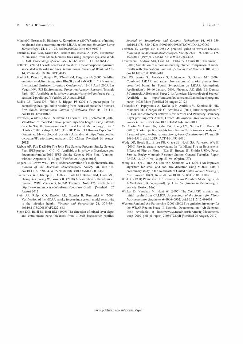
MunkelC, EresmaaN, RasanenA, KarppinenA (2007)Retrieval ofmixing

height and dust concentration with LiDAR ceilometer. Boundary-Layer

Meteorology 124, 117–128. doi:10.1007/S10546-006-9103-3

Pershin S, Hao WM, Susott RA, Babbitt RE, Riebau A (1999) Estimation

of emission from Idaho biomass fires using compact eye-safe diode

LiDAR. Proceedings of SPIE 3757, 60–66. doi:10.1117/12.366438

Potter BE (2005) The role of releasedmoisture in the atmospheric dynamics

associated with wildland fires. International Journal of Wildland Fire

14, 77–84. doi:10.1071/WF04045

Pouliot G, Pierce T, Benjey W, O’Neill SM, Ferguson SA (2005) Wildfire

emission modeling: integrating BlueSky and SMOKE. In ‘14th Annual

International Emission Inventory Conference’, 11–14 April 2005, Las

Vegas, NV. (US Environmental Protection Agency: Research Triangle

Park, NC) Available at http://www.epa.gov/ttn/chief/conference/ei14/

session12/pouliot.pdf [Verified 25 August 2012]

Radke LF, Ward DE, Philip J, Riggan PJ (2001) A prescription for

controlling the air pollution resulting from the use of prescribed biomass

fire: clouds. International Journal of Wildland Fire 10, 103–111.

doi:10.1071/WF01020

Raffuse S,WadeK, Stone J, SullivanD, LarkinN, Tara S, SolomonR (2009)

Validation of modeled smoke plume injection heights using satellite

data. In ‘Eighth Symposium on Fire and Forest Meteorology’, 12–15

October 2009, Kalispell, MT. (Eds BE Potter, TJ Brown) Paper 5A.3.

(American Meteorological Society) Available at https://ams.confex.

com/ams/8Fire/techprogram/paper_156192.htm [Verified 26 August

2012]

Riebau AR, Fox D (2010) The Joint Fire Science Program Smoke Science

Plan. JFSP project 1–C-01–01 Available at http://www.firescience.gov/

documents/smoke/2010_JFSP_Smoke_Science_Plan_Final_Version_

without_Appendix_B_1.0.pdf [Verified 26 August 2012]

Rogers RR, BrownWOJ (1997)Radar observation of amajor industrial fire.

Bulletin of the American Meteorological Society 78, 803–814.

doi:10.1175/1520-0477(1997)078,0803:ROOAMI.2.0.CO;2

Skamarock WC, Klemp JB, Dudhia J, Gill DO, Barker DM, Duda MG,

Huang X-Y, Wang W, Powers JG (2008) A description of the advanced

research WRF Version 3, NCAR Technical Note 475, available at:

http://www.mmm.ucar.edu/wrf/users/docs/arwv3.pdf [Verified 26

August 2012]

Stein AF, Rolph GD, Draxler RR, Stunder B, Ruminski M (2009)

Verification of the NOAA smoke forecasting system: model sensitivity

to the injection height. Weather and Forecasting 24, 379–394.

doi:10.1175/2008WAF2222166.1

Steyn DG, Baldi M, Hoff RM (1999) The detection of mixed layer depth

and entrainment zone thickness from LiDAR backscatter profiles.

Journal of Atmospheric and Oceanic Technology 16, 953–959.

doi:10.1175/1520-0426(1999)016,0953:TDOMLD.2.0.CO;2

Torrence C, Compo GP (1998) A practical guide to wavelet analysis.

Bulletin of the AmericanMeteorological Society 79, 61–78. doi:10.1175/

1520-0477(1998)079,0061:APGTWA.2.0.CO;2

Trentmann J, AndreaeMO, Graf H-F, Hobbs PV, Ottmar RD, Trautmann T

(2002) Simulation of a biomass-burning plume: Comparison of model

results with observations. Journal of Geophysical Research 107, 4013.

doi:10.1029/2001JD000410

Tsai PS, Frasier SJ, Goodrick S, Achtemeier G, Odman MT (2009)

Combined LiDAR and radar observations of smoke plumes from

prescribed burns. In ‘Fourth Symposium on LiDAR Atmospheric

Applications’, 10–16 January 2009, Phoenix, AZ. (Eds BB Demoz,

J Comstock, A Behrendt) Paper 2.1. (AmericanMeteorological Society)

Available at https://ams.confex.com/ams/89annual/techprogram/

paper_147257.htm [Verified 26 August 2012]

Tsaknakis G, Papayannis A, Kokkalis P, Amiridis V, Kambezidis HD,

Mamouri RE, Georgoussis G, Avdikos G (2011) Inter-comparison of

LiDAR and ceilometer retrievals for aerosol and Planetary Boundary

Layer profiling over Athens, Greece. Atmospheric Measurement Tech-

niques 4, 1261–1273. doi:10.5194/AMT-4-1261-2011

Val Martin M, Logan JA, Kahn RA, Leung FY, Nelson DL, Diner DJ

(2010) Smoke injection heights from fires in North America: analysis of

5 years of satellite observations. Atmospheric Chemistry and Physics 10,

1491–1510. doi:10.5194/ACP-10-1491-2010

Wade DD, Brock BL, Brose PH, Grace JB, Hoch GA, Patterson WA III

(2000) Fire in eastern ecosystems. In ‘Wildland Fire in Ecosystems:

Effects of Fire on Flora’. (Eds JK Brown, JK Smith) USDA Forest

Service, Rocky Mountain Research Station, General Technical Report

RMRS-42, Ch. 4, vol. 2, pp. 53–96. (Ogden, UT)

Wang WT, Qu J, Hao XJ, Liu YQ, Sommers WT (2007) An improved

algorithm for small and cool fire detection using MODIS data: a

preliminary study in the southeastern United States. Remote Sensing of

Environment 108(2), 163–170. doi:10.1016/J.RSE.2006.11.009

Weil JC (1988) Plume rise. In ‘Lectures on Air Pollution Modeling’. (Eds

A Venkatram, JC Wyngaard). pp. 119–166. (American Meteorological

Society: Boston, MA)

Winker D, Vaughan M, Hunt W (2006) The CALIPSO mission and

initial results from CALIOP. Proceedings of the Society for Photo-

Instrumentation Engineers 6409, 640902. doi:10.1117/12.698003

Western Regional Air Partnership (2005) 2002 Fire emission inventory for

the WRAP Region Phase II. Essential Documentation. (Air Sciences,

Inc.) Available at http://www.wrapair.org/forums/fejf/documents/

wrap_2002_phii_ei_report_20050722.pdf [Verified 26 August, 2012]

www.publish.csiro.au/journals/ijwf

R Int. J. Wildland Fire Y. Liu et al.