Embed Size (px)
Citation preview

SANDIA REPORT SAND2014-0712 Unlimited Release Printed January 2014
SMART Wind Turbine Rotor: Data Analysis and Conclusions
Jonathan C. Berg, Matthew F. Barone, and Nathanael C. Yoder
Prepared by Sandia National Laboratories Albuquerque, New Mexico 87185 and Livermore, California 94550
Sandia National Laboratories is a multi-program laboratory managed and operated by Sandia Corporation, a wholly owned subsidiary of Lockheed Martin Corporation, for the U.S. Department of Energy's National Nuclear Security Administration under contract DE-AC04-94AL85000. Approved for public release; further dissemination unlimited.

2
Issued by Sandia National Laboratories, operated for the United States Department of Energy
by Sandia Corporation.
NOTICE: This report was prepared as an account of work sponsored by an agency of the
United States Government. Neither the United States Government, nor any agency thereof,
nor any of their employees, nor any of their contractors, subcontractors, or their employees,
make any warranty, express or implied, or assume any legal liability or responsibility for the
accuracy, completeness, or usefulness of any information, apparatus, product, or process
disclosed, or represent that its use would not infringe privately owned rights. Reference herein
to any specific commercial product, process, or service by trade name, trademark,
manufacturer, or otherwise, does not necessarily constitute or imply its endorsement,
recommendation, or favoring by the United States Government, any agency thereof, or any of
their contractors or subcontractors. The views and opinions expressed herein do not
necessarily state or reflect those of the United States Government, any agency thereof, or any
of their contractors.
Printed in the United States of America. This report has been reproduced directly from the best
available copy.
Available to DOE and DOE contractors from
U.S. Department of Energy
Office of Scientific and Technical Information
P.O. Box 62
Oak Ridge, TN 37831
Telephone: (865) 576-8401
Facsimile: (865) 576-5728
E-Mail: [email protected]
Online ordering: http://www.osti.gov/bridge
Available to the public from
U.S. Department of Commerce
National Technical Information Service
5285 Port Royal Rd.
Springfield, VA 22161
Telephone: (800) 553-6847
Facsimile: (703) 605-6900
E-Mail: [email protected]
Online order: http://www.ntis.gov/help/ordermethods.asp?loc=7-4-0#online

3
SAND2014-0712
Unlimited Release
Printed January 2014
SMART Wind Turbine Rotor: Data Analysis and Conclusions
Jonathan C. Berg and Matthew F. Barone
Wind Energy Technologies Department
Sandia National Laboratories
P.O. Box 5800
Albuquerque, New Mexico 87185-MS1124
Nathanael C. Yoder
ATA Engineering
11995 El Camino Real, Suite 200
San Diego, California 92130
Abstract
The Wind Energy Technologies department at Sandia National Laboratories has
developed and field tested a wind turbine rotor with integrated trailing-edge flaps
designed for active control of the rotor aerodynamics. The SMART Rotor project was
funded by the Wind and Water Power Technologies Office of the U.S. Department of
Energy (DOE) and was conducted to demonstrate active rotor control and evaluate
simulation tools available for active control research. This report documents the data
post-processing and analysis performed to date on the field test data.
Results include the control capability of the trailing edge flaps, the combined
structural and aerodynamic damping observed through application of step actuation
with ensemble averaging, direct observation of time delays associated with
aerodynamic response, and techniques for characterizing an operating turbine with
active rotor control.

4
ACKNOWLEDGMENTS
The SMART rotor project was funded by the U.S. Department of Energy (DOE) Wind and
Water Power Technologies Office (director Jose Zayas) under the office of Energy Efficiency
and Renewable Energy (EERE, assistant secretary David Danielson).
The authors gratefully acknowledge all those who contributed to this project, including the
following:
USDA-ARS staff at Bushland Test Site
Adam Holman
Byron Neal
Testing
Wesley Johnson
Bruce LeBlanc
Nate Yoder (ATA Engineering)
Data Acquisition System programming
Juan Ortiz-Moyet (Prime Core)
Blade Modification
David Calkins
Mike Kelly
Bill Miller
Blade Manufacture by TPI Composites
SMART blade design
Matt Barone
Dale Berg
Jonathan Berg
Gary Fischer
Josh Paquette
Brian Resor
Mark Rumsey
Jon White
Consultation
Derek Berry (TPI Composites)
Mike Zuteck (MDZ Consulting)
5
CONTENTS
Executive summary ......................................................................................................................... 9
1. Introduction ............................................................................................................................... 13 1.1 Motivation ......................................................................................................................... 13 1.2 SMART Rotor Experiments ............................................................................................. 14
1.3 Structure of This Report.................................................................................................... 15
2. Aeroelastic Modeling ................................................................................................................ 17 2.1 Aerodynamic Modeling Considerations for SMART Rotors ........................................... 17
2.1.1 Time Scales ......................................................................................................... 17 2.1.2 Unsteady Aerodynamics ...................................................................................... 19
2.2 Aerodynamic Model Choices for SMART Rotors ........................................................... 20
2.2.1 Blade Sectional Models ....................................................................................... 21
2.2.2 Rotor Wake Models ............................................................................................. 22 2.3 Conclusions ....................................................................................................................... 25
3. Field Test Data Analysis ........................................................................................................... 27 3.1 Flap Control Capability..................................................................................................... 27
3.2 Time-Average Response to Step Actuation ...................................................................... 29 3.3 Rotor Dynamics ................................................................................................................ 36
3.3.1 Sine Sweep with Rotor Stopped .......................................................................... 36
3.3.2 Sine Sweep during Power Production ................................................................. 37 3.4 Flap Drive System Dynamics ........................................................................................... 39
3.4.1 Flap Drive with Rotor Stopped ........................................................................... 39 3.4.2 Flap Drive during Power Production ................................................................... 44
3.5 Power Curves .................................................................................................................... 47 3.5 Conclusions ....................................................................................................................... 50
4. Data Acquisition System........................................................................................................... 51 4.1 Introduction ....................................................................................................................... 51 4.2 Channel List ...................................................................................................................... 52 4.3 Time Synchronization ....................................................................................................... 56
4.4 Data Dropouts ................................................................................................................... 58
5. Data Post Processing ................................................................................................................. 59 5.1 Scale and Offset ................................................................................................................ 59 5.2 Coordinate Systems and Transformations ........................................................................ 61 5.3 Time-Synchronized Resampling ....................................................................................... 62
6. On-Ground Calibration ............................................................................................................. 67 6.1 Preliminary Blade Modal Properties ................................................................................. 67
6.2 Preliminary Beam Model Updating .................................................................................. 69 6.3 Blade Strain Calibrations .................................................................................................. 72
7. Blade Surface Geometry ........................................................................................................... 75
8. References ................................................................................................................................. 81
Appendix A: ATLAS Configuration Settings.............................................................................. 87

6
Distribution ................................................................................................................................... 94

7
FIGURES
Figure ES.1 The SMART rotor with photo inset of trailing edge flaps. .........................................9
Figure ES.2 Average strain response showing flap control capability. .......................................10
Figure ES.3 Logarithmic sweep excitation of flapwise acceleration frequencies. ......................11
Figure 3.1 Strain response tracking with flap step sequence. ...................................................28
Figure 3.2 Average strain response as a function of wind speed and flap angle........................28
Figure 3.3 Ensemble average strain response to 20 degree flap step. .......................................30
Figure 3.4 Detail of strain oscillations in step response. ...........................................................30
Figure 3.5 Ensemble average generator power response to 20 degree flap step. ......................31
Figure 3.6 Ensemble average response of rotor fore-aft IMU to 20 degree flap step. ...............32
Figure 3.7 Ensemble average strain response at 6.75 m span. ..................................................33
Figure 3.8 Ensemble average generator power response. .........................................................34
Figure 3.9 Ensemble average rotor IMU response, fore-aft component. ..................................35
Figure 3.10 Parked rotor spectrogram of flapwise acceleration with log sine sweep. ................36
Figure 3.11 Parked rotor PSD of flapwise acceleration with log sine sweep excitation. ............37
Figure 3.12 Power production spectrogram of flapwise acceleration with log sine sweep. .......38
Figure 3.13 Power production PSD of flapwise acceleration with log sine sweep excitation. ...38
Figure 3.14 Sequence of video frames showing blade tip motion during one flap cycle. ..........39
Figure 3.15 Motor current demand during sinusoidal flap motion at 1 Hz. ................................40
Figure 3.16 Flap drive simulation with primarily Coulomb damping. .......................................42
Figure 3.17 Flap drive simulation with primarily viscous damping. ...........................................42
Figure 3.18 Flap drive simulation with numerical instability at two points. ...............................42
Figure 3.19 Motor shaft angle response to log frequency sweep. ...............................................43
Figure 3.20 Amplitude gain and phase shift between motor shaft response and command. ......43
Figure 3.21 Amplitude gain and phase shift between motor current and shaft angle. ................44
Figure 3.22 Motor current demand for various frequencies of sinusoidal motion. .....................45
Figure 3.23 Hinge moment coefficient at 7.8 m span. ................................................................46
Figure 3.24 Flap drive simulation with aerodynamic hinge moment included. ..........................47
Figure 3.25 Power curve at 0 degree flap compared to unmodified rotor. ..................................48
Figure 3.26 Power curve of each flap setting compared to 0 degree setting. ..............................49
Figure 4.1 Example of samples acquired at different rates. ......................................................56
Figure 4.2 Example of sample rate determination. ...................................................................57
Figure 5.1 Orientation of accelerometers with respect to blade coordinate system. .................61
Figure 5.2 Pattern of residuals about straight-line fit to GPS time. ..........................................63
Figure 5.3 Schematic of subsystem clock delays and channel offsets. .....................................64
Figure 6.1 Simple beam element model used to display the experimental mode shapes. ..........68
Figure 6.2 Edgewise blade pull on calibration fixture. ..............................................................73
Figure 7.1 Creaform’s handheld optical scanning system. ........................................................75
Figure 7.2 Point cloud from scan of entire blade surface. . ........................................................75
Figure 7.3 Detail of SMART blade tip with flaps positioned at -20 degrees. ...........................76
Figure 7.4 Comparison of chord distributions. ..........................................................................77
Figure 7.5 Comparison of twist distributions. ...........................................................................77
Figure 7.6 Cross sections at 3 meter span align almost perfectly. ............................................78
Figure 7.7 Cross sections at 5 meter span show variation in thickness. ....................................78
Figure 7.8 Cross sections at 7.2 meter span annotated with SMART blade alterations. ..........79

8
Figure 7.9 Cross sections at 7.9 meter span with variations annotated. ........................................79
TABLES
Table 2.1 Time scales associated with AALC for the Sandia 115kW test turbine. ..................18
Table 3.1 Damped free vibration parameters calculated from strain response. .......................31
Table 4.1 Data acquisition subsystem channel groups. ...........................................................53
Table 4.2 Channel List ....................................................................................................... 54-55
Table 5.1 Summary of post-processing offsets and multipliers. ..............................................60
Table 5.2 Mapping of accelerometer channels to blade coordinate system. ............................61
Table 5.3 Subsystem sample periods in seconds. ....................................................................62
Table 5.4 Channel offsets relative to subsystem clocks. ..........................................................65
Table 6.1 Free-free natural frequency and damping values. ....................................................69
Table 6.2 Comparison of the free-free experimental results and model correlation. ...............70
Table 6.3 Calculated flapwise stiffness distribution. ...............................................................70
Table 6.4 Calculated edgewise stiffness distribution. ..............................................................71
Table 6.5 Average free-free frequencies of experiment and model compared. .......................71
Table 6.6 Blade strain calibration results. ................................................................................72

9
EXECUTIVE SUMMARY
The Wind Energy Technologies department at Sandia National Laboratories has developed and
field tested a wind turbine rotor with integrated trailing-edge flaps, seen in Figure ES.1, designed
for active control of rotor aerodynamics. Analysis of the field test data has focused on addressing
the following goals of the project:
Demonstrate the control capability of the trailing-edge flaps.
Evaluate the accuracy of simulation tools in predicting results of active rotor control.
Develop procedures for characterizing an operating wind turbine which has active rotor
control.
Figure ES.1 The SMART rotor consists of three 9-meter blades with trailing edge flaps spanning 20% of each blade length. The photo
inset is a closer look at the flaps on one blade.
Control capability of the trailing-edge flaps was observed in the blade strain response.
Figure ES.2 shows how the change in microstrain with wind speed shifts up or down by about 40
microstrain when the flaps are positioned at the +20 or -20 degree actuation limits. This change
in strain at 6.75 m span is roughly equivalent to the amount of strain induced when the turbine
goes from parked to operational. In 9 m/s wind, the blade strain at 6.75 m span during power
production differs from the non-operational strain by 35 microstrain. Thus, the average observed
control capability (measured at three-quarters blade span) with maximum flap deflection was
roughly 114% of the strain that results from typical flapwise loading during power production.

10
Figure ES.2 Average strain response as a function
of wind speed shifts up and down with flap actuation angle.
The transient response of the wind turbine to step motions of the flaps was observed for the
purpose of comparison to the response predicted by simulation tools. Analysis of blade strain
step response revealed a combined aerodynamic and structure damping on the order of 1% to 3%
of critical damping. Damping added by aerodynamic forces is typically difficult to quantify and
this result shows step excitation is an effective method of system characterization.
Analysis of response time delays revealed the generator power step response reached peak value
about 0.3 seconds after the flap step transition occurred. In this amount of time the rotor turned
about one-third of a revolution and the wake moved downwind approximately one-eighth of a
rotor diameter (assuming the wake was travelling at 8 m/s). This observation and the overall
character of the step response are important results for evaluating the accuracy of simulation
tools which support active aerodynamic control research.
Analysis of response time delays revealed the blade strain step response was delayed by 0.02
seconds, which is consistent with the expected amount of time required for the local blade
section airflow to adjust to perturbations. This result also supports evaluation of simulation tools.
Aero-elastic system dynamics of the operational turbine system were observed in the frequency
domain. Dynamics were heavily influenced by the effects of aerodynamic forces which add
damping. Figure ES.3 shows the peak system response occurred at 4.4 Hz when the logarithmic
sine sweep crossed this frequency at around 500 seconds. The vertical lines are multiples of the
turbine’s rotational frequency (55 rpm or 0.92 Hz). The logarithmic sine sweep was shown to be
a useful tool for system characterization.
4 6 8 10 12-150
-100
-50
0
50
100
Wind Speed (m/s)
Change in m
icro
str
ain
B2_H2_Strain_6750_Z_HP
20 deg
15 deg
10 deg
5 deg
0 deg
-5 deg
-10 deg
-15 deg
-20 deg

11
Figure ES.3 Excitation of flapwise acceleration frequencies over time with logarithmic sine sweep of flaps showing peak system response at 4.4 Hz.
Flap drive system dynamics were analyzed by using actuator current as an approximate
measurement of the aerodynamic hinge moments acting on the flaps. A simple actuator model
revealed the role of Coulomb (friction) and viscous damping in the flap drive system response.
Frequency response of the flap actuation system was calculated and discussed in relation to the
reduced frequency of unsteady aerodynamic response. These observations are important for the
success of future closed-loop active rotor control.
Power curves for the SMART rotor were measured and compared to the power curve of a
baseline CX-100 rotor. Effect of flap position on power was observed. These results are
important to understand tradeoffs between energy capture and active aerodynamic load control.

12
NOMENCLATURE
AAD active aerodynamic device
AALC active aerodynamic load control
ATLAS Accurate GPS Time-Linked Acquisition System
chordwise in the direction of airfoil chord and perpendicular to blade span
dB decibel
DOE Department of Energy (U.S.)
edgewise similar to chordwise but used to describe blade loads and deflections
flapwise perpendicular to edgewise and in the direction of blade “flapping” motion
GBU Ground-Based Unit (data acquisition subsystem)
GPS global positioning system
HP high-pressure (the nominally upwind surface of a HAWT blade)
IMU inertial measurement unit
inboard toward the root end of a wind turbine blade
LE leading edge of wind turbine blade
LP low-pressure (the nominally downwind surface of a HAWT blade)
outboard toward the tip of a wind turbine blade
PID proportional-integral-derivative
PSD power spectral density
RBU Rotor-Based Unit (data acquisition subsystem)
R&D research and development
SFID sequential frame ID
SMART Structural and Mechanical Adaptive Rotor Technology
SNL Sandia National Laboratories
spanwise in the direction of the blade length
TE trailing edge of wind turbine blade
TEF trailing edge flaps

13
1. INTRODUCTION
1.1 Motivation
As the United States seeks to establish a diverse portfolio of clean and renewable energy
systems, continued development of wind energy technology is essential to reaching renewable
energy deployment goals. The Report on the First Quadrennial Technology Review (QTR),
published by the U.S. Department of Energy in September 2011, was written to “establish a
framework for thinking clearly about a necessary transformation of the Nation’s energy system”
[1]. The QTR was a first step in developing guiding principles for DOE to prioritize investment
of R&D funds. Within the “Clean Electricity Generation” strategy outlined in the report, wind
energy is described as a fairly mature technology which is cost competitive at good wind sites
and continues to expand market deployment. At a high-level assessment, the report states the
technical headroom for additional research and development exists mainly in grid integration and
subsystem reliability as well as tapping into the offshore wind resource.
The 20% Wind Energy by 2030 report [2], published in July 2008, provides a more detailed
assessment of the technical headroom for additional R&D. The core opportunities it identifies
include reducing capital costs, increasing capacity factors, and mitigating risk through enhanced
system reliability. The rotor itself is highlighted as a key target for technology improvement
because it is the source of all energy captured and of most of the structural loads entering the
system. Increasing rotor size while controlling rotor loads will directly impact the capacity factor
and the life of components within the main load path. The report mentions both passive load
control in which the structural and material properties of the blades are tailored to passively
mitigate loads and active load control in which a control system senses rotor loads and actively
responds by driving aerodynamic actuators.
Reducing ultimate and oscillating (or fatigue) loads on the wind turbine rotor can lead to
reductions in loads on other turbine components such as the main bearings, gearbox, and
generator. This, in turn, is expected to reduce maintenance costs and may also allow a given
turbine to use longer blades to capture more energy. In both cases, the ultimate impact is reduced
cost of wind energy. With the ever increasing size of wind turbine blades and the corresponding
increase in non-uniform loads along the span of those blades, the need for more sophisticated
load control techniques has produced great interest in the use of aerodynamic control devices
(with associated sensors and control systems) distributed along each blade to provide feedback
load control (often referred to in popular terms as ‘smart structures’ or ‘smart rotor control’). A
review of concepts and inventory of design options for such systems have been performed by
Barlas and van Kuik at Delft University of Technology (TU Delft) [3]. Active load control
utilizing trailing edge flaps or deformable trailing edge geometries is receiving significant
attention because of the direct lift control capability of such devices. Researchers at TU Delft [4-
5], Risø/Danish Technical University Laboratory for Sustainable Energy (Risø/DTU) [6-12] and
Sandia National Laboratories (SNL) [13-19] have been active in this area over the past decade.

14
1.2 SMART Rotor Experiments
The Sandia SMART rotor project was conducted to demonstrate active control of wind turbine
rotor aerodynamics and evaluate the simulation tools which support research in this area. The
design and construction, which took place in 2010 and 2011, are documented in reference [20].
This report describes the results of the field test which was conducted in 2012.
The SMART rotor was tested on a modified Micon 65/13 which is a single-speed stall controlled
(fixed-pitch) turbine. Each SMART blade was 9 meters long and was equipped with trailing edge
flaps which spanned 20% of the blade length. The rigid flaps were hinged at 20% of chord and
were actuated by electric motors. See reference [20] for additional information on the test site
and test turbine.
Similar full scale turbine experiments were conducted by Risø DTU in collaboration with Vestas
Wind Systems A/S on a V27 wind turbine [21, 22]. The Vestas V27 is a dual-speed pitch
controlled turbine with 13 meter long blades and a nominal power output of 225 kW. One of the
three blades had been equipped with trailing edge flaps (TEF) which spanned 15% of the blade
length. The TEF were flexible in the first round of tests conducted in 2010 as described in
reference [21]. As mentioned in reference [22], the TEF were changed to a stiff hinged flap
design for the tests conducted in 2011.
Reference [21] describes three types of measurement configurations that were used:
Trailing edge flaps fixed in neutral positions.
Trailing edge flaps fixed in alternating low lift and high lift configurations.
Trailing edge flaps actuated at a given frequency.
Testing showed the flap motions could alter the blade root flap-wise bending moment by 1 to 2%
of the mean flap-wise moment. The flexibility of the flaps in the first round of tests increased
modeling uncertainty because the TEF shape could deflect under aerodynamic load. Actuation at
a given frequency increased the blade root moment power spectral density at the excitation
frequency and also produced a coupled response in the other two blades at a slightly higher
frequency.
Reference [22] describes closed-loop control of the TEF with a frequency-weighted model
predictive controller. Technical issues prevented operation of the two inner flaps and so the one
working flap spanned only 5% of the blade length. An average load reduction of 14% was
reported for a test 38 minutes in duration.

15
1.3 Structure of This Report
The primary information, analysis, and conclusions are contained in Chapters 2 and 3 with
additional explanation and supporting information in the subsequent chapters and appendix.
Chapter 2 discusses aero-elastic modeling considerations and choice of models for simulation of
active aerodynamic rotor control. Chapter 3 presents analysis of the field test data and resulting
conclusions. Chapters 4 and 5 describe the data acquisition system and required data post
processing. Chapters 6 and 7 describe ground test model calibration data and blade surface
geometry scans.

16

17
2. AEROELASTIC MODELING
Simulation strategies and design tools have evolved to allow rapid prediction of performance and
loads for modern horizontal-axis wind turbines. The aerodynamic components of these models,
while not uniformly accurate for every turbine operating condition, have been in use for some
time, and their behavior and regions of validity are fairly well-understood. The SMART rotor
concept involves a fundamental change in rotor aerodynamic characteristics, since now
aerodynamic properties may be dynamically changed at different locations along the blade span
by active aerodynamic load control (AALC) devices. Also, the time scale of AALC device
actuation is shorter than that of variable full-blade pitch. These differences may require
modifications to existing wind turbine aerodynamic analysis tools, and may possibly require the
development of new models of aerodynamic phenomena specific to AALC operation.
This chapter considers the aerodynamics of SMART rotor technology and implications for
aerodynamic modeling. Existing aerodynamic modeling approaches are surveyed, and
modifications or areas of need for new approaches are identified. This work does not provide a
detailed review of all available modeling approaches for wind turbine aerodynamics. There are
several good reviews from the past decade that cover this subject, including [23] and [24]. The
emphasis here is on models capable of predicting:
Aerodynamic loads that contribute to fatigue loading under turbulent wind conditions
Blade aerodynamic response to AALC device actuation.
2.1 Aerodynamic Modeling Considerations for SMART Rotors
2.1.1 Time Scales
There are several relevant physical time scales, or groups of time scales, involved in wind
turbine load control using AALC devices. Understanding these time scales gives insight into the
underlying physical processes as well as the ability to assess the validity of various modeling
approaches.
The first group of time scales is associated with excitation of the wind turbine aero-elastic
system. The excitation inputs to the system include both the turbulent wind input and actuation
of the AALC devices. The wind turbulence contains broadband velocity fluctuations, with
energy distributed over a continuous range of time scales (and spatial scales). Some of this
fluctuation energy occurs at time scales comparable to the wind turbine aero-elastic time scales.
This leads to efficient excitation of the wind turbine structure, resulting in dynamic deflections of
the blades and tower along with associated fatigue loads. Spatial variations in the mean wind
speed due to wind shear, as well as low-frequency turbulent fluctuations that vary in space across
the rotor plane, also lead to excitation of the wind turbine at multiples of the rotational
frequency.
The device actuation time scale, on the other hand, is associated with the frequency of operation
of the AALC device. The achievable range of the device actuation time scale is device-
dependent. However, for effective load control the device time scale range needs to include the

18
time scales of important excitation inputs, including the rotational frequency, its harmonics and
possibly higher frequency wind events.
The second set of time scales is associated with the structural modes of the wind turbine system;
these modes include blade modes (flapwise, torsional, edgewise), tower modes, coupled modes,
and full system modes. Each mode has a natural frequency with an associated time scale.
Typically, the lowest-frequency structural modes are the most important in determining dynamic
response and loads. In application of AALC devices, reduction of flapwise fatigue loads is
usually a primary goal, although care must be taken to avoid excessive excitation of torsional and
edgewise modes by the AALC system.
The third set of time scales is associated with aerodynamic phenomena on actively controlled
blades. A local blade section flow time scale is associated with the time for a particle to travel
the local chord length at the local relative flow velocity, or tf = c/Urel. A related aerodynamic
time scale is the time for the local two-dimensional flow over a blade section to adjust to a
sudden perturbation, such as an instantaneous change in angle of attack or AALC device
deployment. This time scale is usually at least several times the local section flow time scale. A
third aerodynamic time scale is the wake response time, or the time for the velocity field induced
by the rotor trailing vorticity to adjust to a sudden change in blade aerodynamic load distribution.
When considering the wake response of a load change on the entire rotor, this time scale is
usually much longer than the local section flow time scale, since it is proportional to the ratio of
rotor radius to the wind velocity.
Table 2.1 shows estimates of various time scales for the Sandia 115kW test turbine operating at
55 RPM with a wind speed of 8 m/s. The center of the AALC flapped section is located at 89%
of the rotor radius, which is where the local section flow time scale is estimated. The range of
AALC device actuation time scales is assumed to include the period of the first two blade
flapwise modes, as well as the periods associated with the rotational frequency and two
harmonics of the rotational frequency (1P,2P,3P). It is assumed the AALC devices are actuating
in response to wind fluctuations that cause structural excitation at these frequencies.
Table 2.1 Time scales associated with active aerodynamic control
for the Sandia 115kW test turbine.
Process Time Scale Definition Time Scale
AALC Device Actuation Actuation Period 0.09 – 1.1 sec Response to Rotationally Sampled
Wind 1P,2P,3P periods 0.3 - 1.1 sec
Dynamic Structural Response Period of First Two Blade Flap
Modes 0.09 - 0.22 sec
Local Section Flow Chord / Relative Flow Velocity 0.004 sec Local Section Flow Adjustment 5-10x Section Flow Time Scale 0.02 - 0.04 sec
Wake Response Rotor Radius / Wind Speed 1.2 sec
19
2.1.2 Unsteady Aerodynamics
The interactions between wind turbulence, aerodynamic loads, and structural dynamics give rise
to the fatigue loads that AALC devices seek to control. The turbulent wind and AALC device
actuation serve as inputs to the overall aero-elastic system. Aerodynamic forces and moments
(aerodynamic loads) are generated in response to these inputs. The aerodynamic loads, in turn,
excite the structural dynamic modes, which lead to structural fatigue loading. Structural modes
may also couple with one another, changing the structural loading. Further, structural motion
modifies the aerodynamic loads, resulting in a two-way coupled system.
To simplify the arguments, consider only a one-way coupling in which inputs lead to
aerodynamic loads, which in turn lead to dynamic structural loads. A key question is whether
assumptions of large separation of the aerodynamic and structural dynamic time scales are valid.
If these time scales are sufficiently far apart, then the aerodynamics can be assumed to occur
nearly instantaneously (termed a quasi-steady assumption), simplifying the required aerodynamic
models.
Recall that there are several aerodynamic time scales, two of which are most relevant to the
present discussion: the local flow adjustment time scale, and the wake response time scale.
Consider first the local flow adjustment time scale. At first glance, for the Sandia 115kW test
turbine, the flow appears to adjust fairly quickly compared to the actuation and structural time
scales (0.04 second versus 0.09-1.1 seconds). However, this qualitative observation is not
sufficient to ensure that a quasi-steady assumption of the aerodynamic loads is valid. What also
must be determined is whether the aerodynamic response to an unsteady excitation is quasi-
steady. In other words, are the amplitude and phase of the aerodynamic loads in response to wind
turbulence or AALC device actuation well-approximated by the steady-state response at each
point in time during the transient?
This question can be answered by examining the reduced frequency of the excitation. The
reduced frequency k is defined by
(2.1)
where ω is the circular frequency of the excitation, c is the local blade chord length, and Urel is
the local flow velocity relative to the blade section. The reduced frequency is essentially a scaled
ratio of the flow time scale to the excitation time scale. The aerodynamic response to unsteady
excitation is a function of the reduced frequency. For small reduced frequencies, the response is
essentially quasi-steady, while for large reduced frequencies the response is highly unsteady and
deviates substantially from the quasi-steady response, both in phase and amplitude. Leishmann
[23] states that an unsteady aerodynamic system can only be considered quasi-steady for k <
O(0.01). For k < 0.05, errors due to the quasi-steady assumption are likely acceptable for wind
turbine aero-elastic system modeling. Note that this implies the flow time scale must be almost
two orders of magnitude less than the excitation time scale for the quasi-steady assumption to
hold. For higher reduced frequencies, the unsteady aerodynamic loading will differ from that of
the quasi-steady case, with possibly important implications for determining structural loads and
aero-elastic stability.

20
The reduced frequency range of the AALC excitation for the Sandia test turbine at 89% radius is
calculated as 0.01 < k < 0.2. The low end of the estimated reduced frequency range is associated
with the 1P disturbance, which can be caused by wind shear or tower shadow. Note that 1P loads
can be effectively reduced using individual blade pitch control [25]. If the primary action of the
AALC devices is to control 1P loads, then a quasi-steady aerodynamic model is probably
sufficient. If the AALC devices are actuating on time scales associated with blade mode natural
frequencies, or 3P or higher rotational harmonics, the estimate indicates that the quasi-steady
assumption is not strictly valid (0.06 < k < 0.2). In this case, an unsteady aerodynamic model for
the response to turbulent wind and AALC device actuation should be used.
The rotor wake response is seen to occur over a time scale of about 1.2 seconds. Note that this
corresponds to roughly one rotor revolution; it may actually take five or more rotor revolutions
for the wake, once perturbed, to settle into a steady state. The relevant reduced frequency for this
case uses the rotor radius and wind speed to non-dimensionalize the frequency, rather than the
blade chord and local relative velocity. A caveat is that wake and inflow time scales vary along
the blade, and are shorter for the outboard part of the blade than for the inboard part. This can be
accounted for in an approximate way by using the wake time scale distribution function from the
wake model of Snel [26]. Another consideration is that only the outboard part of the blade, the
part containing the AALC devices, is undergoing unsteady aerodynamic changes. Thus, a more
relevant length scale for computing reduced frequency is the AALC device span. Assuming a
device span of 20% of the blade centered about r/R = 0.89 for the SMART rotor, the reduced
frequency of the wake response using the expected AALC actuation frequency is in the range
0.25 < k < 2.5. The reduced frequencies are again such that the quasi-steady assumption is poor.
This means a dynamic wake model is necessary to resolve changes in blade aerodynamic loading
due to turbulent wind and/or AALC device actuation.
In summary, estimates for reduced frequency associated with wind turbine structural excitation
and AALC actuation indicate:
A quasi-steady aerodynamic model may be sufficient for excitation at the rotational
frequency.
For excitation at higher harmonics of the rotational frequency, or direct excitation of
blade modes by high frequency turbulent energy, an unsteady aerodynamic model is
required.
For modeling of the effect of aerodynamic wake response to wind turbulence or AALC
device actuation, a dynamic wake model is required.
2.2 Aerodynamic Model Choices for SMART Rotors
The aerodynamic modeling of a wind turbine rotor is usually divided into two components: blade
sectional modeling and wake modeling. The blade sectional models predict local aerodynamic
forces and moments for two-dimensional sections of the blades given local flow properties such
as angle of attack and relative velocity. The wake models (also called “inflow models”) predict
the velocity induced by the trailing vorticity in the rotor wake. The two models are coupled since

21
the wake model affects the inputs to the sectional aerodynamic model, while the section model
provides aerodynamic load distributions that determine the strength and shape of the wake.
The previous section outlined the need for dynamic models for both the blade section and the
wake aerodynamics. This section discusses some of the available models and their
appropriateness for SMART rotor applications.
2.2.1 Blade Sectional Models
In the usual blade element approach, the blade is divided into airfoil sections, or elements, and
the static two-dimensional aerodynamic characteristics of each element are described using lift,
drag, and pitching moment tables defined across the relevant range of angle of attack and chord
Reynolds number. For airfoil sections with AALC devices, tables also need to be derived for the
static performance of the airfoils with devices deployed. Unsteady aerodynamic effects can be
accounted for by using thin-airfoil theory and the relevant potential flow solutions [23]. For
airfoil sections with trailing edge AALC devices, the theory can be modified to account for
unsteady actuation of the devices. This has been done for devices that change trailing edge
camber (flaps or morphing trailing edge) [27] as well as for miniature Gurney flap (or “micro-
tab”) devices [28].
For large device actuation amplitude and frequency, or for large or rapid changes in the incident
angle of attack, a nonlinear model describing the dynamic stall process must be included. There
is some question regarding the importance of modeling dynamic stall properly for SMART
rotors. Under turbine operating conditions with small yaw error and “usual” stochastic
atmospheric turbulence levels, the outboard region of a variable-pitch rotor should not be stalled,
either statically or dynamically. This assumption has been justified by full system aero-elastic
simulations [25]. In these conditions, modeling of dynamic stall is not important in determining
the ability of AALC devices to reduce fatigue loads. However, when analyzing the performance
of AALC devices and a SMART rotor control system under non-ideal operating conditions, such
as at large yaw angle, properly modeling dynamic stall is important. Dynamic stall models for
some AALC devices, including a morphing trailing edge and microtabs, have been developed
[28, 29].
Various three-dimensional flow effects must be accounted for by modification of the two
dimensional airfoil models for analysis of wind turbine blades. Rotational augmentation [30]
increases lift and delays stall to higher angle of attack, due to the effects of blade rotation on the
boundary layer. This effect is most important on the inboard portion of the blade, and is of
secondary importance to modeling the aerodynamics of AALC devices, which will most likely
be placed on the outboard part of the blade. The three-dimensional flow induced by the blade tip
vortex does affect the outboard part of the blade. Models for this effect are available in the form
of “tip-loss” models (see, e.g., [31]), although these do not account for the presence of outboard
control surfaces. The AALC devices themselves can generate trailing vortices which may
interact with the tip vortex and thus change the local aerodynamic behavior. More analysis
and/or experimentation is needed to determine the importance of this effect and appropriate
modeling strategies.

22
In summary, the primary components of blade sectional aerodynamic models for SMART rotor
fatigue analysis include:
1. Static airfoil performance tables with and without AALC device deployment
2. Unsteady airfoil aerodynamic model (from thin airfoil theory, for example)
3. Unsteady AALC device aerodynamic model (modification to thin airfoil theory)
4. Dynamic stall model for airfoil with AALC devices, for analysis of non-ideal operating
conditions
5. Tip-loss model, possibly modified for interaction with AALC devices
2.2.2 Rotor Wake Models
Wake models for SMART rotors must include dynamic wake effects, as discussed in Section
2.1.2. This precludes the use of an equilibrium wake model such as the classical Blade Element
Momentum (BEM) model. Variants of the BEM model have been developed that include
dynamic wake effects. One such model is presented in [26], where the wake is approximated by
a cylindrical vortex sheet extending from the rotor plane to an infinite distance downstream of
the turbine. A dynamic equation for induction velocity at the rotor plane is derived using
vorticity/velocity relationships and balancing changes in blade forces with changes in trailed
vorticity. This results in a relatively simple differential equation model for unsteady induced
velocity at the rotor axis; it can also be modified to give an induced velocity distribution across
the rotor disc. There are some theoretical limitations to models based on the BEM foundation.
For the model in [26], the blade load distribution is assumed to be linear with radius, which leads
to a constant load per swept area. Further, implementations of this type of model assume the
momentum balance takes place in an averaged sense over an annular region of the rotor. It is not
clear that this approach is valid for analysis of a wind turbine operating in turbulent wind, where
significant instantaneous variations in wind speed may occur across the rotor.
Dynamic Inflow Models
An alternative approach to wake modeling follows the method of “Dynamic Inflow” (DI)
initiated by Pitt and Peters [32]. The DI modeling framework has led to a family of models,
including the Finite State Induced Flow model [33]. A particular implementation of this type of
model is the Generalized Dynamic Wake (GDW) model, described in [34], and implemented in
the Aerodyn code [35].
Both the DI and GDW models are based on the actuator disc concept. An actuator disc is an
infinitesimally thin region, coincident with the rotor plane, over which aerodynamic forces are
assumed to act on the surrounding flow. The actuator disc concept itself is fairly general, in that
it only provides a means for modeling the action of aerodynamic blade loads. The flow dynamics
are then modeled using any number of methods, ranging from simple potential flow models to
numerical solutions of the Navier-Stokes equations. The DI and GDW models are based on the
linearized momentum equation (and continuity equation) governing inviscid, incompressible
flow.
23
The momentum equation is linearized about a uniform free-stream, and solutions are found for
the induced flow distribution normal to the rotor plane. Because of the linearization, the induced
flow is assumed to be a small perturbation to the free-stream flow. For a wind turbine, this means
the model is strictly valid only for small values of the axial induction factor, a << 1.
The pressure field for linearized, inviscid, incompressible flow satisfies LaPlace’s equation. The
pressure field in the DI and GDW models is based on the work of Kinner (see [36]), who found
solutions to LaPlace’s equation that contain a discontinuity in pressure across a circular disc. A
general solution for pressure can be expanded in an infinite sum involving products of Legendre
polynomials and azimuthal Fourier components. The aerodynamic blade loads are similarly
expanded in a spectral basis, and are used to force the surrounding pressure field solution.
The GDW model has the advantage that it is derived from the momentum equation, so in this
sense it is a first-principles approach, within the constraints of the applied linearization. While
the model is not explicitly based on vortex dynamics, the Kinner solution field in the wake will
include vorticity [36]. However, due to the linearization, the model is essentially a prescribed
wake method and will not describe non-linear behavior such as vortex roll-up.
The assumption of small induction factor involved in the linearization of the momentum
equation is the primary limitation of the model. The model would be expected to be accurate for
lightly-loaded rotor conditions. Unfortunately, wind turbine induction factors are usually
relatively large, with the optimum induction factor for an ideal rotor being a = 1/3.
The GDW model is quite general in allowing for arbitrary blade loadings and induced velocity
distributions. Practically, the allowable loadings and velocity distributions are limited by the
number of terms retained in the pressure field, velocity field, and blade load expansions. Thus,
sharp flow features that may occur due to step changes in spanwise loading, such as occurs at the
blade tips or at the edge of aerodynamic control surfaces, will not be captured precisely unless a
very large number of terms is included. The implementation of the GDW model in Aerodyn
includes four azimuthal harmonics and four Legendre polynomials in the radial direction. The
number of polynomials would likely need to be increased in order to model SMART rotors,
increasing the cost and complexity of the model.
Free Vortex Wake Models
The flow in the wake of a lifting surface such as a wind turbine blade is often best described in
terms of vortices and their dynamics. This motivated the relatively simple wake model discussed
earlier [26], in which the wake is modeled as a semi-infinite vortex sheet. A vortex sheet is an
example of a singular potential flow solution used to describe part of a wake flow; other potential
flow elements include vortex filaments and vortex particles. When the position of the potential
flow elements is kept fixed at pre-determined positions in space, the model is called a prescribed
wake model. Prescribed wake models require advance knowledge of the wake shape, which in
the general case must be determined experimentally. For relatively simple configurations, such
as a turbine in steady, uniform, axial flow, prescribed wake models can be very accurate.
However, for more complex flow conditions, uncertainty in the geometry of the wake leads to
inaccuracies.

24
A prescribed wake model may not make a good choice for modeling a turbine with active
aerodynamic load control. First, the model would need to provide an accurate description of the
wake under turbulent wind conditions in order to furnish fatigue load predictions. Under
turbulent wind conditions, the wind velocity varies across the rotor disc and as a function of
time, which may cause local distortions of the wake geometry that are not accounted for in the
prescribed wake method. Second, the AALC devices may induce local changes in aerodynamic
blade loading that cause perturbations to the wake geometry. For small enough perturbations this
effect may be negligible, but this should be verified by comparisons to a more accurate wake
model.
An alternative is to use methods where the wake geometry is free to evolve in space and time.
These methods usually use vortex elements as the computational building blocks, and are called
free vortex methods (FVM). Free vortex methods have been popular in the rotorcraft community
for some time [37], and have also been applied to horizontal axis wind turbines [38 – 42]. In one
variant, the vortex filament method, vorticity in the wake of a turbine blade is tracked using
curved filaments representing concentrations of vorticity. This includes the important tip vortex,
trailed from the blade tips, as well as weaker trailing vortices resulting from non-uniform
circulation (along the span). Changes in local section circulation produce shed vortices, oriented
parallel to the blade trailing edge. Non-uniform circulation and unsteady sectional lift both occur
under turbulent wind conditions. Non-uniform spanwise circulation can occur when AALC
devices are actuated, creating step change in blade loadings. All of these effects, in principle, are
addressed by the FVM.
Other FVM’s besides the vortex filament method include the vortex particle method [38], vortex
sheet method [43], and hybrids that include some combination of vortex elements [38, 43].
Usually, the FVM is combined with a lifting line method for describing the distribution of
loading along the blade. The lifting line is a bound vortex fixed to the blade that models the lift
distribution, and from which the trailing and shed vortex elements emanate. It can be tied to
sectional airfoil models such as those described in Section 3.1 that account for unsteady sectional
aerodynamics, dynamic stall, and unsteady AALC device actuation. The FVM can also be
combined with a Navier-Stokes CFD solution in the near field of the rotor blades, as described in
[44]. Although this method may result in computational savings over a CFD model of the entire
rotor flow-field, it is not yet practical for design or fatigue load calculations.
One detail of potential flow wake models that may be important for SMART rotors is the issue
of non-planar wake behavior. The wake of a blade or wing just downstream of the trailing edge
is usually well-described by a thin, planar sheet attached to the trailing edge. An AALC device
may perturb the wake such that the wake is no longer planar. An example is the wake of a
trailing edge flap with non-flapped blade sections on either side of the flap. The flap displaces
the wake above or below the unflapped wake position, resulting in a discontinous wake
geometry. A planar wake assumption in this case can lead to inaccuracies in blade load
predictions. This limitation can be overcome by incorporating a non-planar wake method [45].
One aspect of the FVM that has hindered widespread use in wind turbine design is its
computational cost. For a simulation with N vortex elements, the computational cost is

25
proportional to N2, since the induced velocity from each element must be calculated at every
other element position. There are algorithms for computing the velocity field that scale linearly
with N, such as the fast multipole method [46]. This method was applied to vortex particle
simulations in [43], but can also be applied to vortex filament methods [47]. Some run times
were reported in [43] for various FVM methods. It is not clear if FVM methods are yet practical
for running wind turbine fatigue load cases (multiple 10-minute turbulent wind simulations, for
example). A study of the required computational resources to accomplish this would be very
useful.
Summary of Wake Models
In summary, the following are important considerations for choice of a rotor wake model for
simulating SMART rotors:
Models based on BEM theory usually employ averaging over annular regions of the rotor
disc, and may not properly resolve important instantaneous spatial variations in blade
loading.
Dynamic inflow models, within the constraints of the assumption of small induction
factor, can simulate arbitrary inflow distributions associated with turbulent wind
excitation and/or AALC device actuation. However, the method converges relatively
slowly with increases in degrees-of-freedom (DOFs) and may become inefficient when
enough DOFs are retained to resolve the wake of AALC devices.
Free vortex wake models offer a general framework for describing SMART rotor wake
dynamics, and their use in this application would be limited primarily by considerations
of computational cost.
2.3 Conclusions
The analysis of Section 2.1.2 indicates that unsteady aerodynamic models are needed for
SMART rotor analysis. This is not surprising given that much of the rationale for using unsteady
aerodynamic models for SMART rotors is relevant for analysis of turbulence-induced fatigue
loads, a standard design case. Other considerations particular to SMART rotor modeling have
been identified, however. These include airfoil sectional models that incorporate unsteady
aerodynamic modeling of the device actuation, as well as dynamic wake models that are able to
account properly for the shed and trailed vorticity generated by the devices. The sectional models
are currently available for some devices, but may need to be tailored to the particular device
geometry of interest. The required wake models are also available, but selection of a particular
model involves tradeoffs between accuracy and computational expense. The free vortex wake
methods involve fewer assumptions than other techniques and therefore offer the potential for
greater accuracy, but care must be taken that they can be efficiently employed in fatigue analyses
which may involve long simulation times.

26

27
3. FIELD TEST DATA ANALYSIS
Analysis of the field test data has focused on addressing the following goals of the project:
Demonstrate the control capability of the trailing-edge flaps.
Evaluate the accuracy of simulation tools in predicting results of active rotor control.
Develop procedures for characterizing an operating wind turbine which has active rotor
control.
This chapter references the concepts of aerodynamic time scale and reduced frequency which
were presented in Chapter 2.
3.1 Flap Control Capability
The primary type of flap motion that was used to characterize the control capability of the flaps
was a sequence of step motions between the 0 degree position and ± 5, 10, 15, and 20 degrees.
The duration of each step assumed one of two configurations. First, the duration was 2.18
seconds which is nominally two rotor revolutions. In this configuration, all the flap positions
were cycled through quickly which allowed a rapid characterization of the overall control
capability. Second, the duration of each step was extended to 30 seconds so that transient
aerodynamic response would reach steady state before another step motion was initiated.
Figure 3.1 shows the strain response of the most outboard foil strain gage located at 6.75 m span.
Overlaid on the strain response is the commanded flap position (to facilitate comparison, the
strain data has been scaled to be of similar magnitude). The correlation between change in strain
and change in flap angle is clearly visible, although turbulent wind conditions had a pronounced
effect on strain as well. The curves in Figure 3.2 were produced by binning the data according to
wind speed and then averaging the strain response for each flap position. The zero degree flap
curve shifts up or down by about 40 microstrain when the flaps are positioned at the +20 or -20
degree actuation limits. This change in strain at 6.75 m span is roughly equivalent to the amount
of strain induced when the turbine goes from parked to operational. In 9 m/s wind, the blade
strain at this span during power production differs from the non-operational strain by 35
microstrain. Thus, the average observed control capability (measured at three-quarters blade
span) with maximum flap deflection was roughly 114% of the strain that results from typical
flapwise loading during power production.
The overall character of these curves matched the expectations from simulation. Simulation
predicted that the control capability on the positive flap angle side would be somewhat less than
the control capability on the negative flap angle side due to the upper limit on lift coefficient and
the initiation of stall with high positive flap angles. This effect can be seen in Figure 3.2 where
the change in strain for the -20 and +20 degree settings relative to the 0 degree setting are
respectively 50 and 33 microstrain.
Similar results were obtained for the other three strain gage locations but with decreasing ranges
of change in strain. For the -20 and +20 degree settings, one-half blade span saw changes of 44.7

28
and 31.6 microstrain, one-quarter blade span saw changes of 25 and 14.6 microstrain, and the
root saw changes of 4.3 and 2.9 microstrain. The decreasing range was largely the result of blade
stiffness increasing toward the root. At the root, average strain during power production differs
from the non-operational strain by about 8 microstrain. Because the strain at a particular span
location results from all load outboard of that location, the active control portion of the blade
contributes most of the load experienced at three-quarters span but contributes proportionally
less at the root.
Figure 3.1 Strain response tracking with flap step sequence.
Figure 3.2 Average strain response as a function of wind speed shifts up and down with flap actuation angle.
410 420 430 440 450 460-40
-20
0
20
40
Time (s)
B2_H2_Strain_6750_Z_HP
Strain (scaled)
Flap Angle (deg)
4 6 8 10 12-150
-100
-50
0
50
100
Wind Speed (m/s)
Change in m
icro
str
ain
B2_H2_Strain_6750_Z_HP
20 deg
15 deg
10 deg
5 deg
0 deg
-5 deg
-10 deg
-15 deg
-20 deg

29
3.2 Time-Average Response to Step Actuation
A sequence of step motions between the 0 degree flap position and ± 5, 10, 15, and 20 degrees
was also employed to characterize the overall system response. The duration of each step was
extended to 30 seconds so that transient aerodynamic response would reach steady state before
another step motion was initiated. The strain response to each step with the 30 second duration is
similar to the results observed in Figure 3.1 for the shorter duration steps.
The ensemble average of many such responses to the same flap motion revealed the mean flap
response hidden beneath the stochastic wind excitation responses. This time-averaging was
accomplished by first aligning the signals with a “trigger window” centered on the flap angle
signal at a specified trigger level. Then the signals were resampled with a consistent time vector
and averaged.
The following results are focused on the 20 degree flap step response and used a trigger level of
19 degrees. The time axis is aligned so that the flap angle passes through the trigger level at 0.0
seconds. Rise time for the flap step motion was around 0.1 seconds with an average actuation
rate of about 200 degrees per second and a maximum rate of 330 degrees per second.
Figure 3.3 shows the strain signals of 29 individual responses to the 20 degree step motion.
Although the random wind excitation produced a wide band of data which is plotted in gray,
consistent structure in the data is evident in the first second after the step transition. The structure
was clearly revealed in the average of these 29 responses which is plotted as the thin black line.
Figure 3.4 focuses on the first 1.5 seconds of this mean response. The time delay between the
flap motion and strain response was about 0.02 seconds, which appears to be consistent with the
aerodynamic time scale associated with local section flow adjustment. Although the response
was not strictly a “damped free vibration” due to the presence of both constant and random wind
excitation, application of the theory for damped free vibration provided some insight into the
response. First, the frequency of vibration was calculated from the time between peaks to be
4.17 Hz which matches the first flapwise blade bending mode. Second, the damping ratio ζ for
damped free vibration can be calculated from the logarithmic decrement [48], here denoted by δ
in equation (3.1). The logarithmic decrement is simply the natural logarithm of the ratio ui / ui+1
of two successive peak values. If ζ is small such that the denominator in the right hand
expression of equation (3.1) is approximately 1, then the damping ratio can be easily calculated
from equation (3.2). Using these equations, a damping ratio on the order of 1% to 3% of critical
was calculated from the peaks seen in Figure 3.4 using the information contained in Table 3.1.
Damping added by aerodynamic forces is typically difficult to quantify and this result shows step
excitation is an effective method of system characterization.
√ (3.1)
(3.2)

30
Figure 3.3 Ensemble average strain response to 20 degree flap step.
Figure 3.4 Detail of strain oscillations in step response.

31
Table 3.1 Damped free vibration parameters calculated from strain response.
Peak Maximum Time, s Peaks Log
Decrement Damping
Ratio Time
Difference, s 1/ ΔT, s-1
u1 30.38 0.0799 u2 – u1 0.202 0.032 0.2396 4.17
u2 24.83 0.3195 u3 – u2 0.097 0.015 0.2397 4.17
u3 22.54 0.5592 u4 – u3 0.080 0.013 0.2396 4.17
u4 20.81 0.7988
Using the same time-averaging procedure, the ensemble average response of generator power
seen in Figure 3.5 reveals a subtle jump in power output which begins to rise at approximately
0.15 seconds on the trigger window time axis and reaches peak value at 0.3 seconds. In 0.3
seconds the rotor turned about one-third of a revolution and the wake moved downwind
approximately one-eighth of a rotor diameter (assuming the wake was travelling at 8 m/s). This
time delay observation and the overall character of the step response are important results for
evaluating the accuracy of simulation tools which support active aerodynamic control research.
Looking at the individual power output signals plotted in gray in Figure 3.5, the jump is visible
in many of them; however, the amount of variation between signals suggests that attempting to
draw any additional conclusions from the mean response may be asking too much. It is likely
that more than 29 response signals need to be averaged and the variation in wind speed needs to
be taken into account in order to accurately identify other repeatable dynamics being exhibited
here.
Figure 3.5 Ensemble average generator power response to 20 degree flap step
reveals delayed jump in power output.
Signals from the inertial measurement unit (IMU) mounted on the rotor were also examined
using the time-averaging approach. Plotted in Figure 3.6, the z-component, which senses fore-aft

32
tower motion, shows that a substantial ringing was induced at tower top approximately 0.05
seconds after the flap step motion.
It is interesting to note that the rotor thrust response occurs before the generator power (and by
implication the rotor torque) shows any sign of change. Temporal alignment of signals was
double checked to verify the effect was real and not a post-processing error. Timing of the IMU
signals were verified against the rotor azimuth. Timing of the channel which measured the
generator power signal was verified through post-testing of the data acquisition system; however,
phase shift possibly caused by the power transducer itself is unknown but believed to be zero.
Barring a timing issue, the result indicates that rotor thrust is the cumulative effect of local
section flow adjustment and therefore occurs along the same time scale. Rotor power and torque,
however, appear to be directly tied to changes in the rotor wake which occur at the longer wake-
response time scale. The change in induction factor resulting from the delayed wake response
may explain the small reversal of oscillation observed in Figure 3.6 from 0.2 to 0.5 seconds, but
the reversal might also be simply a secondary frequency of tower top motion.
Figure 3.6 Ensemble average response of fore-aft (axial) component of rotor IMU to 20 degree flap step.
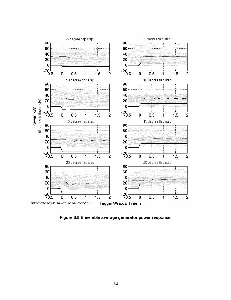
Ensemble averages were computed for strain, power, and rotor IMU acceleration at the other flap
step magnitudes and are shown in Figures 3.7 through 3.9. Results followed the same trends as
seen previously with similar time delays. The -20 degree flap steps just happened to sample wind
with less speed fluctuation and the individual responses are seen to be tightly grouped with a
rather clean ensemble average, particularly in the case of generator power.

33
Figure 3.7 Ensemble average strain response at 6.75 m span.
34
Figure 3.8 Ensemble average generator power response.

35
Figure 3.9 Ensemble average rotor IMU response, fore-aft (axial) component.

36
3.3 Rotor Dynamics
3.3.1 Sine Sweep with Rotor Stopped
Sinusoidal flap motion with logarithmic sweep of frequency was used to provide a driving force
over a range of frequencies. With the rotor parked, the inertia of the flap motion generated the
controlled frequency input while the ambient inflow created a small random buffeting input on
the flat of the blade. Figure 3.10 is the spectrogram of flapwise acceleration during a test which
swept over the frequency range 0.1 to 10 Hz in 500 seconds. The main red portion is the
logarithmic frequency input and the vertical lines are structural resonance frequencies. The other
curves following the shape of the red curve are harmonics of the main input frequency.
Broadband frequency input up to about 15 Hz is visible in the background due to the random
wind buffeting. The power spectral density (PSD) of this same test for all three blades, given in
Figure 3.11, shows a more refined view of the individual frequency response peaks.
Figure 3.10 Parked rotor spectrogram (waterfall plot) of flapwise acceleration at 8000 mm span with logarithmic sine sweep excitation.
37
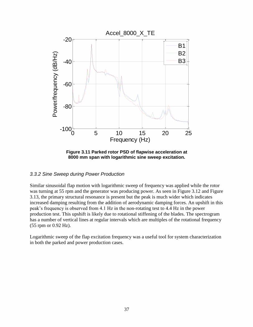
Figure 3.11 Parked rotor PSD of flapwise acceleration at 8000 mm span with logarithmic sine sweep excitation.
3.3.2 Sine Sweep during Power Production
Similar sinusoidal flap motion with logarithmic sweep of frequency was applied while the rotor
was turning at 55 rpm and the generator was producing power. As seen in Figure 3.12 and Figure
3.13, the primary structural resonance is present but the peak is much wider which indicates
increased damping resulting from the addition of aerodynamic damping forces. An upshift in this
peak’s frequency is observed from 4.1 Hz in the non-rotating test to 4.4 Hz in the power
production test. This upshift is likely due to rotational stiffening of the blades. The spectrogram
has a number of vertical lines at regular intervals which are multiples of the rotational frequency
(55 rpm or 0.92 Hz).
Logarithmic sweep of the flap excitation frequency was a useful tool for system characterization
in both the parked and power production cases.
0 5 10 15 20 25-100
-80
-60
-40
-20Accel_8000_X_TE
Frequency (Hz)
Pow
er/
frequency (
dB
/Hz)
B1
B2
B3

38
Figure 3.12 Power production spectrogram (waterfall plot) of flapwise acceleration at 8000 mm span with logarithmic sine sweep.
Figure 3.13 Power production PSD of flapwise acceleration at 8000 mm span with logarithmic sine sweep.
0 5 10 15 20 25-40
-30
-20
-10
0
10Accel_8000_X_TE
Frequency (Hz)
Pow
er/
frequency (
dB
/Hz)
B1
B2
B3

39
Hub mounted video cameras pointed toward the blade tips were used to capture the tip motion
during some of the test runs including one power production sine sweep test. Figure 3.14 is a
sequence of still images over one flap cycle when the blade was excited at the main resonance
frequency. The blade tip is initially downwind or to the left (frame 1) when the flaps begin
moving toward the lower pressure surface. The reduced lift results in tip movement upwind or to
the right (frame 5). As the flaps move back to their initial position, the blade tip also moves back
to the initial position (frame 9).
Figure 3.14 This sequence of video frames of a sinusoidal flap motion shows the blade tip moving from a downwind position (1) to an upwind position (5) and back to the
downwind position (9) during one flap cycle.
3.4 Flap Drive System Dynamics
The flaps were actuated in various motions, both with and without the rotor spinning, to
characterize the motor drive system.
3.4.1 Flap Drive with Rotor Stopped
A simple sinusoidal flap motion of fixed amplitude and frequency was the first step to obtain the
loads on the flap motors in the absence of significant aerodynamic forces. The electrical current
demanded by the motor controllers was expected to result mainly from the torque required to
overcome friction and accelerate the flaps to track the desired flap position.
Figure 3.15 plots the motor current demand against motor shaft angle during a 1 Hz sinusoidal
motion with 5 degree amplitude. (The empty subplots indicate data acquisition failures.)

40
Figure 3.15 Motor current demand during sinusoidal flap motion at 1 Hz frequency and 5 degree amplitude (with parked rotor).
A simple mass-spring-damper model of the flap drive system was constructed to help understand
the key parameters contributing to the observed behavior. The equation of motion for this one
degree-of-freedom rotational system was obtained by application of Newton’s second law:
( ) ( )
The flap angle, speed, and acceleration are represented by and respectively. The
acceleration term coefficient, J, represents the lumped rotational inertia of the flap and other
rotating components. The first damping term coefficient, cviscous, represents viscous-type damping
proportional to the rate of angular motion. The second damping term coefficient, ccoulomb,
represents Coulomb-type damping which depends only on the direction of angular motion. The
“spring force” term, Taero, was chosen to represent the aerodynamic hinge moment acting on the
flap and was given by a nonlinear function. Although other spring-like forces could exist they

41
can be treated as negligible or rolled into the aerodynamic torque term. The final term, Tmotor, is
the torque applied by the motor and it is determined by a PID controller which regulates the
motor shaft position.
The electrical current required by the motor is proportional to its shaft torque and depends on the
following motor parameters:
Motor torque constant, km = 0.0346 Nm/A
Gear ratio, N = 66.22
Gearhead efficiency,
(
) (
)
The relative contribution of viscous and Coulomb damping was estimated by varying each
damping coefficient in the model. The aerodynamic hinge moment term was set to zero for any
simulations with the turbine rotor stopped.
Figure 3.16 shows how the flap drive model responded to changes in Coulomb damping. In the
absence of any significant viscous damping, the shape of the current-angle cycle was rectangular.
The upper left and lower right corners of the cycle have small oscillations where the flap motion
was changing directions. (The oscillation at 0 degree shaft angle was a startup transient in the
simulation.)
Figure 3.17 shows how the flap drive model responded to changes in viscous damping. In the
absence of any significant Coulomb damping, the shape of the current-angle cycle was elliptical.
Viscous damping tended to reduce oscillations and improve numerical stability of the model.
The field test results given in Figure 3.15 show a mostly rectangular cycle which indicates that
Coulomb damping was likely the primary force involved and ccoulomb must be about 0.3 to make
the simulation model match the results. However, there were obviously other dynamics involved
to produce the observed results. Wind loading may have been a factor and the motor controller
itself may have produced some of the oscillatory behavior. In the simulation model, gains of the
PID controller were tuned and scaling parameters were adjusted until some additional features
appeared in the cycle. Figure 3.18 shows one case in which the controller tended to respond a bit
chaotically at the upper left and lower right corners of the cycle. This somewhat matches the
observed behavior but was likely the result of numerical stability issues. Additional modelling
efforts would be required to obtain a tuned simulation model.
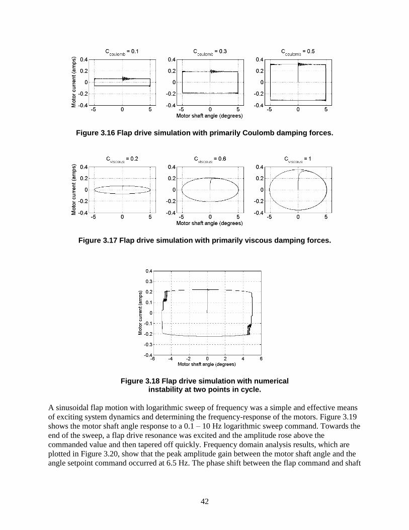
42
Figure 3.16 Flap drive simulation with primarily Coulomb damping forces.
Figure 3.17 Flap drive simulation with primarily viscous damping forces.
Figure 3.18 Flap drive simulation with numerical instability at two points in cycle.
A sinusoidal flap motion with logarithmic sweep of frequency was a simple and effective means
of exciting system dynamics and determining the frequency-response of the motors. Figure 3.19
shows the motor shaft angle response to a 0.1 – 10 Hz logarithmic sweep command. Towards the
end of the sweep, a flap drive resonance was excited and the amplitude rose above the
commanded value and then tapered off quickly. Frequency domain analysis results, which are
plotted in Figure 3.20, show that the peak amplitude gain between the motor shaft angle and the
angle setpoint command occurred at 6.5 Hz. The phase shift between the flap command and shaft
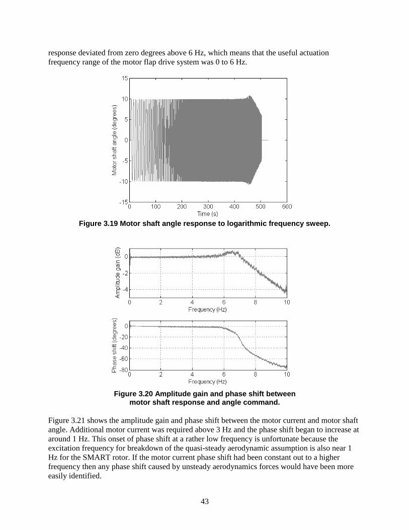
43
response deviated from zero degrees above 6 Hz, which means that the useful actuation
frequency range of the motor flap drive system was 0 to 6 Hz.
Figure 3.19 Motor shaft angle response to logarithmic frequency sweep.
Figure 3.20 Amplitude gain and phase shift between
motor shaft response and angle command.
Figure 3.21 shows the amplitude gain and phase shift between the motor current and motor shaft
angle. Additional motor current was required above 3 Hz and the phase shift began to increase at
around 1 Hz. This onset of phase shift at a rather low frequency is unfortunate because the
excitation frequency for breakdown of the quasi-steady aerodynamic assumption is also near 1
Hz for the SMART rotor. If the motor current phase shift had been constant out to a higher
frequency then any phase shift caused by unsteady aerodynamics forces would have been more
easily identified.

44
Figure 3.21 Amplitude gain and phase shift between
motor current and motor shaft angle.
3.4.2 Flap Drive during Power Production
With the rotor spinning and producing power, the flap controller was stepped through a series of
sinusoidal flap motions each with a different frequency. The electrical current demanded by the
motor controllers was expected to be a combination of aerodynamic forces and other effects such
as friction in the flap drive system.
Figure 3.22 plots the motor current demand against motor shaft angle for Blade 3. Frequency of
the sinusoidal motions ranged from 0.1 Hz to 6 Hz and the amplitude was 5 degrees. A transition
occurs in the shape of the current-angle cycles between the actuation frequencies of 0.8 and 1.5
Hz. The reduced frequency of the flap excitation was calculated as described in Section 2.1.2 to
be 0.001 < k < 0.08. The 0.8 Hz sinusoidal motion has a reduced frequency of about 0.01 which
corresponds to the upper limit O(0.01) for a quasi-steady aerodynamic assumption. However, it
must be noted again that the phase shift between motor current and motor shaft angle also begins
to increase at around 1 Hz excitation frequency and thus the onset of unsteady aerodynamic
behavior cannot be easily identified from motor current phase. Additional testing must be
performed with appropriate measurements; these measurements may include aerodynamic
inflow, surface pressure, or actuator current (assuming the actuator’s inherent phase relationship
can be chosen to avoid interference).

45
Figure 3.22 Motor current demand for various frequencies
of sinusoidal motion (during power production).
At low frequencies, the rectangular shape caused by Coulomb damping was again the
predominant characteristic. However, with aerodynamic forces involved, the rectangle became a
rhomboid which was skewed along a trendline with positive slope.
The aerodynamic hinge moment in the simulation model was represented by a nonlinear function
of the flap angle. Using XFOIL [49], the hinge moment about the flap hinge line was estimated
for a range of operating conditions and flap angles. Figure 3.23 shows the hinge moment
coefficient at three angles of attack for the airfoil at 7.8 m span. Similar results were obtained
inboard and outboard of this span location and so, for simplicity, only one equation for the
moment coefficient was carried forward. The quadratic fit line is given by equation (3.3).

46
( ) ( ) ( ) (3.3)
The hinge moment varies with span according to equation (3.4), where ρ is the air density, V is
the local air velocity, and c is the chord length.
( ) (3.4)
Figure 3.23 Hinge moment coefficient at 7.8 m span.
In the flap drive simulation model, the following fixed parameters were chosen:
Air density ρ = 1.088 kg/m3
Chord c = 0.2613 m
Wind speed of 9 m/s, which produces a local air velocity (at 8.6 m radius)
of V = 50.32 m/s
Total scale factor
Nm (per meter span)
The length of each flap was 2 feet or 1.8288 meters.
Combining these parameter values with equations (3.3) and (3.4), the flap drive simulation
model produced a similar rhomboid shape for motor current versus shaft angle. However, the
result was offset by about 0.5 amps in the positive direction on the vertical axis. Zeroing out the
last term in equation (3.3) brought the results back down into the range observed in Figure 3.22.
It is not clear why the predicted offset in motor current did not appear in the data. One possibility
is that the flap angle differs from the motor shaft angle measurement and therefore equation (3.3)
must be offset with respect to the flap angle argument rather than zeroing out the constant offset
term. An offset of -10 degrees between the motor shaft angle and flap angle would shift the curve
in Figure 3.23 to the right and produce roughly the same effect as shifting the curve down by

47
0.005 amps. Video of the flaps during turbine operation did reveal a flap offset in the negative
angle direction but the amount of offset cannot be judged accurately.
Ideally, the angle of the flap itself would have been measured but the space constraints and
project timeline prevented integration of dedicated angle sensors for the flaps. In addition, the
linkage mechanism between the motor and flap could be redesigned to reduce the possibility of
relative motion.
Having addressed the offset issue, the simulation parameters were then adjusted to obtain similar
rhomboid side lengths. The Coulomb damping coefficient needed to be increased from 0.3 to 0.4,
which could be explained by increased lateral force on the flap hinge causing the sleeve bearing
friction to rise. A viscous damping coefficient in the range of 0.1 to 0.3 appeared to produce a
similar rounded top to the rhomboid. Figure 3.24 shows the simulation result at three different
frequencies of sinusoidal motion.
Figure 3.24 Flap drive simulation with aerodynamic hinge moment included.
The shape was roughly captured at lower actuation frequencies where the assumption of quasi-
steady aerodynamics applies and the inherent motor current phase shift was small. Additional
analysis and modelling efforts would be required to obtain a tuned flap drive simulation model
which captures the observed frequency dependence.
3.5 Power Curves
The following power curves were obtained from 5 hours of test data acquired on a single day.
The wind direction ranged from approximately 170 to 260 degrees with an average direction of
214.5 degrees which matches the site’s prevailing wind direction of 215 degrees. Thus, the
center meteorological tower was directly in line with the turbine.
The hub height wind cup, BAHHC, provided the wind speed measurement for the power curves.
Computing the cross-correlation with the nacelle wind cup, the average time delay for the wind
to reach the turbine was 3.62 seconds. This time delay was applied to the wind speed signal to
minimize error when reporting the generator power measurements versus wind speed.
A sequence of step motions between the 0 degree flap position and ± 5, 10, 15, and 20 degrees
was employed to spread the wind speed distribution evenly among the various flap positions.

48
The duration of each step was 30 seconds and the first 2 seconds of data after the step transition
was discarded to remove the initial power transients.
Figure 3.25 compares the SMART rotor’s generator power at the 0 degree flap setting with the
generator power of a previous CX-100 test. A power loss ranging from 7 to 15% was
experienced and early initiation of stall is evident at around 13 m/s. The bend in the power curve
below 6 m/s was likely caused by inaccuracy of the wind cup at low wind speeds due to friction
and inertia.
Figure 3.25 Power curve at 0 degree flap compared to unmodified rotor.
Figure 3.26 shows the power output at each flap position. Positive flap angles produced roughly
the same power with some excursions having an 8 to 14% increase. Negative flap angles
produced noticeable decreases in power ranging from -5 kW at -10 degree flap to -10 kW at -20
degree flap. Of particular interest are the stall behaviors observed for the 10 degree and -15
degree flap settings. It is not clear why the 10 degree setting consistently initiated an early blade
stall whereas the 15 and 20 degree settings behaved much the same as the 0 degree setting.
The -15 degree setting appears to have three groups of points at stall which may be related to
dynamic stall effects.

49
Figure 3.26 Power curve of each flap setting compared to the 0 degree setting.

50
3.5 Conclusions
The control capability of the trailing-edge flaps was observed in the blade strain response at
three-quarters span and was shown to be roughly 114% of the strain at this span that results from
power production thrust loads. Influence on strain at the blade root was roughly 50% of the strain
that results from power production thrust loads.
Transient response of the wind turbine to step motions of the flaps showed that step excitation is
an effective method of system characterization which revealed a combined aerodynamic and
structure damping on the order of 1% to 3% of critical damping. Response time delays were
observed which are important for evaluating the accuracy of simulation tools that support active
aerodynamic research.
The logarithmic sine sweep was shown to be a useful tool for system characterization of both the
operational turbine and the flap drive subsystem. Methods to obtain accurate models of the
system dynamics are important for the success of future closed-loop active rotor control.

51
4. DATA ACQUISITION SYSTEM
4.1 Introduction
Understanding the architecture of the data acquisition system that was used in this project is
critical for understanding the required signal processing. The system consisted of four
acquisition subsystems each having an independent clock. Because the clocks were independent,
the timing of data samples was not completely synchronized between the subsystems. In
addition, within each subsystem some of the data channels exhibited an additional time offset
relative to the other subsystem channels. All of these timing characteristics are documented in
the following tables and discussion. The four subsystems are now described briefly and
identified by name.
The first subsystem was physically located at ground level in the “ground-based-unit” or GBU.
This unit acquired all signals on the non-rotating side of the turbine and also signals from the
meteorological towers. The other three subsystems were physically located on the rotor in the
“rotor-based-unit” or RBU.
The GBU subsystem hardware was a KAM-500 from ACRA Control [50] and was named
“GBU”. The first of the three RBU subsystems was another KAM-500 unit which was named
“ACRA” and the second RBU subsystem was a cRIO-9025 from National Instruments [51]
which was named “cRIO”. The third RBU subsystem was an sm130 fiber optic interrogator from
Micron Optics [52] which was named “Micron Optics Interrogator” or “MOI”. Additional
information on the subsystem hardware modules and software configuration can be found in the
Appendix A on ATLAS Configuration Settings.
In the turbine control building, a desktop computer running the ATLAS II software package [53]
controlled the four subsystems and merged their four data streams together. “ATLAS” stands for
“Accurate GPS Time-Linked Acquisition System” and the software had originally been
developed to work with the ACRA-based hardware subsystems to enable time-linked acquisition
from systems that could not be physically linked to each other. The idea was to use GPS
technology to provide an accurate time source to synchronize data instead of a physical hardware
“trigger”. Special hardware was developed for the ACRA subsystems to integrate GPS time into
their data acquisition capabilities.
For the more recent Sensor Blade and SMART Rotor tests, ATLAS was modified to also
incorporate data from the National Instruments cRIO-9025 and Micron Optics sm130. A S.E.A.
[54] GSM / GPS Communication Module (cRIO Gxxx+) provided the GPS time source for the
cRIO. Although the MOI does not have a GPS input, the cRIO handles its data acquisition and
thus the two subsystems have essentially the same sample clock.
Although the GPS time-linking strategy implemented in ATLAS was adequate for the LIST
campaign [55] – which relied mostly on ten-minute averages – it was discovered that the ATLAS
software employed in the Sensor Blade and SMART Rotor tests did not provide direct sample-
to-sample alignment between the four subsystem data streams. Fortunately, in the SMART Rotor
test, some of the sensor signals where shared between the cRIO and ACRA to provide a way to

52
re-align the data streams. In addition, the rotor’s inertial measurement unit (IMU) detected the
rotor’s orientation with respect to gravity and thus provided a surrogate for the rotor azimuth
signal measured by the GBU and a way to re-align the GBU and RBU subsystems.
4.2 Channel List
This section provides a brief overview of the list of channels acquired during the SMART Rotor
field test. The purpose is to provide a point of reference for discussion of data channels in
subsequent sections and to highlight the signals which are most important for the resampling and
realignment post-processing steps.
Table 4.1 organizes the channels by the four subsystems previously described and, within each
subsystem, identifies the following groups: GPS signals, Sync signals (data frame
synchronization), general sensor signals, and specific sensor signals important for realignment.
These alignment signals are the following: Azimuth and IMU, Blade 1 Strains (shared signals
between ACRA and cRIO), and Impact Hammer (shared signal between ACRA and cRIO).
To distinguish between the subsystem clocks in data post-processing, each clock was given a
“Clock ID” number ranging from one to three. The cRIO, ACRA, and GBU were given clock ID
numbers 1, 2, and 3, respectively. Because the MOI sampling was handled by the cRIO, it also
used Clock ID 1.
Table 4.2 presents the full list of channels.

53
Table 4.1 Data acquisition subsystem channel groups.
Subsystem Channel Description Subsystem
Clock ID
1 TimeStamp 1
GBU
2 .. 5 <gbu sync>
3
6 .. 21 <gbu signals>
22 AZIMUTH_ANGLE
23 .. 38 <gbu signals>
39 .. 43 <gbu gps>
ACRA
44 .. 47 <acra sync>
2
48 .. 54 B1 Strains
55 .. 97 <acra signals>
98 .. 100 DAQ_IMU
101 Impact Hammer
102 .. 106 <acra gps>
cRIO
107 .. 110 <crio sync>
1
111 .. 115 <crio gps>
116 .. 139 <crio signals>
140 .. 146 B1 Strains
147 .. 149 DAQ_IMU
150 Impact Hammer
MOI 151 .. 186 <moi signals> 1
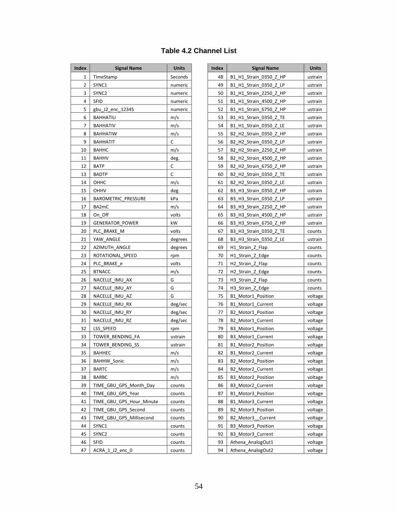
54
Table 4.2 Channel List
Index Signal Name Units
Index Signal Name Units
1 TimeStamp Seconds
48 B1_H1_Strain_0350_Z_HP ustrain
2 SYNC1 numeric
49 B1_H1_Strain_0350_Z_LP ustrain
3 SYNC2 numeric
50 B1_H1_Strain_2250_Z_HP ustrain
4 SFID numeric
51 B1_H1_Strain_4500_Z_HP ustrain
5 gbu_J2_enc_12345 numeric
52 B1_H1_Strain_6750_Z_HP ustrain
6 BAHHATIU m/s
53 B1_H1_Strain_0350_Z_TE ustrain
7 BAHHATIV m/s
54 B1_H1_Strain_0350_Z_LE ustrain
8 BAHHATIW m/s
55 B2_H2_Strain_0350_Z_HP ustrain
9 BAHHATIT C
56 B2_H2_Strain_0350_Z_LP ustrain
10 BAHHC m/s
57 B2_H2_Strain_2250_Z_HP ustrain
11 BAHHV deg.
58 B2_H2_Strain_4500_Z_HP ustrain
12 BATP C
59 B2_H2_Strain_6750_Z_HP ustrain
13 BADTP C
60 B2_H2_Strain_0350_Z_TE ustrain
14 OHHC m/s
61 B2_H2_Strain_0350_Z_LE ustrain
15 OHHV deg.
62 B3_H3_Strain_0350_Z_HP ustrain
16 BAROMETRIC_PRESSURE kPa
63 B3_H3_Strain_0350_Z_LP ustrain
17 BA2mC m/s
64 B3_H3_Strain_2250_Z_HP ustrain
18 On_Off volts
65 B3_H3_Strain_4500_Z_HP ustrain
19 GENERATOR_POWER kW
66 B3_H3_Strain_6750_Z_HP ustrain
20 PLC_BRAKE_M volts
67 B3_H3_Strain_0350_Z_TE counts
21 YAW_ANGLE degrees
68 B3_H3_Strain_0350_Z_LE ustrain
22 AZIMUTH_ANGLE degrees
69 H1_Strain_Z_Flap counts
23 ROTATIONAL_SPEED rpm
70 H1_Strain_Z_Edge counts
24 PLC_BRAKE_e volts
71 H2_Strain_Z_Flap counts
25 BTNACC m/s
72 H2_Strain_Z_Edge counts
26 NACELLE_IMU_AX G
73 H3_Strain_Z_Flap counts
27 NACELLE_IMU_AY G
74 H3_Strain_Z_Edge counts
28 NACELLE_IMU_AZ G
75 B1_Motor1_Position voltage
29 NACELLE_IMU_RX deg/sec
76 B1_Motor1_Current voltage
30 NACELLE_IMU_RY deg/sec
77 B2_Motor1_Position voltage
31 NACELLE_IMU_RZ deg/sec
78 B2_Motor1_Current voltage
32 LSS_SPEED rpm
79 B3_Motor1_Position voltage
33 TOWER_BENDING_FA ustrain
80 B3_Motor1_Current voltage
34 TOWER_BENDING_SS ustrain
81 B1_Motor2_Position voltage
35 BAHHEC m/s
82 B1_Motor2_Current voltage
36 BAHHW_Sonic m/s
83 B2_Motor2_Position voltage
37 BARTC m/s
84 B2_Motor2_Current voltage
38 BARBC m/s
85 B3_Motor2_Position voltage
39 TIME_GBU_GPS_Month_Day counts
86 B3_Motor2_Current voltage
40 TIME_GBU_GPS_Year counts
87 B1_Motor3_Position voltage
41 TIME_GBU_GPS_Hour_Minute counts
88 B1_Motor3_Current voltage
42 TIME_GBU_GPS_Second counts
89 B2_Motor3_Position voltage
43 TIME_GBU_GPS_Millisecond counts
90 B2_Motor3__Current voltage
44 SYNC1 counts
91 B3_Motor3_Position voltage
45 SYNC2 counts
92 B3_Motor3_Current voltage
46 SFID counts
93 Athena_AnalogOut1 voltage
47 ACRA_1_J2_enc_0 counts
94 Athena_AnalogOut2 voltage
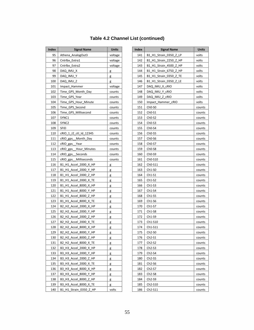
55
Table 4.2 Channel List (continued)
Index Signal Name Units
Index Signal Name Units
95 Athena_AnalogOut3 voltage
141 B1_H1_Strain_0350_Z_LP volts
96 Cntrlbx_Extra1 voltage
142 B1_H1_Strain_2250_Z_HP volts
97 Cntrlbx_Extra2 voltage
143 B1_H1_Strain_4500_Z_HP volts
98 DAQ_IMU_X g
144 B1_H1_Strain_6750_Z_HP volts
99 DAQ_IMU_Y g
145 B1_H1_Strain_0350_Z_TE volts
100 DAQ_IMU_Z g
146 B1_H1_Strain_0350_Z_LE volts
101 Impact_Hammer voltage
147 DAQ_IMU_X_cRIO volts
102 Time_GPS_Month_Day counts
148 DAQ_IMU_Y_cRIO volts
103 Time_GPS_Year counts
149 DAQ_IMU_Z_cRIO volts
104 Time_GPS_Hour_Minute counts
150 Impact_Hammer_cRIO volts
105 Time_GPS_Second counts
151 Ch0-S0 counts
106 Time_GPS_Millisecond counts
152 Ch0-S1 counts
107 SYNC1 counts
153 Ch0-S2 counts
108 SYNC2 counts
154 Ch0-S3 counts
109 SFID counts
155 Ch0-S4 counts
110 cRIO_1_J2_ctl_Id_12345 counts
156 Ch0-S5 counts
111 cRIO_gps__Month_Day counts
157 Ch0-S6 counts
112 cRIO_gps__Year counts
158 Ch0-S7 counts
113 cRIO_gps__Hour_Minutes counts
159 Ch0-S8 counts
114 cRIO_gps__Seconds counts
160 Ch0-S9 counts
115 cRIO_gps__Milliseconds counts
161 Ch0-S10 counts
116 B1_H1_Accel_2000_X_HP g
162 Ch0-S11 counts
117 B1_H1_Accel_2000_Y_HP g
163 Ch1-S0 counts
118 B1_H1_Accel_2000_Z_HP g
164 Ch1-S1 counts
119 B1_H1_Accel_2000_X_TE g
165 Ch1-S2 counts
120 B1_H1_Accel_8000_X_HP g
166 Ch1-S3 counts
121 B1_H1_Accel_8000_Y_HP g
167 Ch1-S4 counts
122 B1_H1_Accel_8000_Z_HP g
168 Ch1-S5 counts
123 B1_H1_Accel_8000_X_TE g
169 Ch1-S6 counts
124 B2_H2_Accel_2000_X_HP g
170 Ch1-S7 counts
125 B2_H2_Accel_2000_Y_HP g
171 Ch1-S8 counts
126 B2_H2_Accel_2000_Z_HP g
172 Ch1-S9 counts
127 B2_H2_Accel_2000_X_TE g
173 Ch1-S10 counts
128 B2_H2_Accel_8000_X_HP g
174 Ch1-S11 counts
129 B2_H2_Accel_8000_Y_HP g
175 Ch2-S0 counts
130 B2_H2_Accel_8000_Z_HP g
176 Ch2-S1 counts
131 B2_H2_Accel_8000_X_TE g
177 Ch2-S2 counts
132 B3_H3_Accel_2000_X_HP g
178 Ch2-S3 counts
133 B3_H3_Accel_2000_Y_HP g
179 Ch2-S4 counts
134 B3_H3_Accel_2000_Z_HP g
180 Ch2-S5 counts
135 B3_H3_Accel_2000_X_TE g
181 Ch2-S6 counts
136 B3_H3_Accel_8000_X_HP g
182 Ch2-S7 counts
137 B3_H3_Accel_8000_Y_HP g
183 Ch2-S8 counts
138 B3_H3_Accel_8000_Z_HP g
184 Ch2-S9 counts
139 B3_H3_Accel_8000_X_TE g
185 Ch2-S10 counts
140 B1_H1_Strain_0350_Z_HP volts
186 Ch2-S11 counts
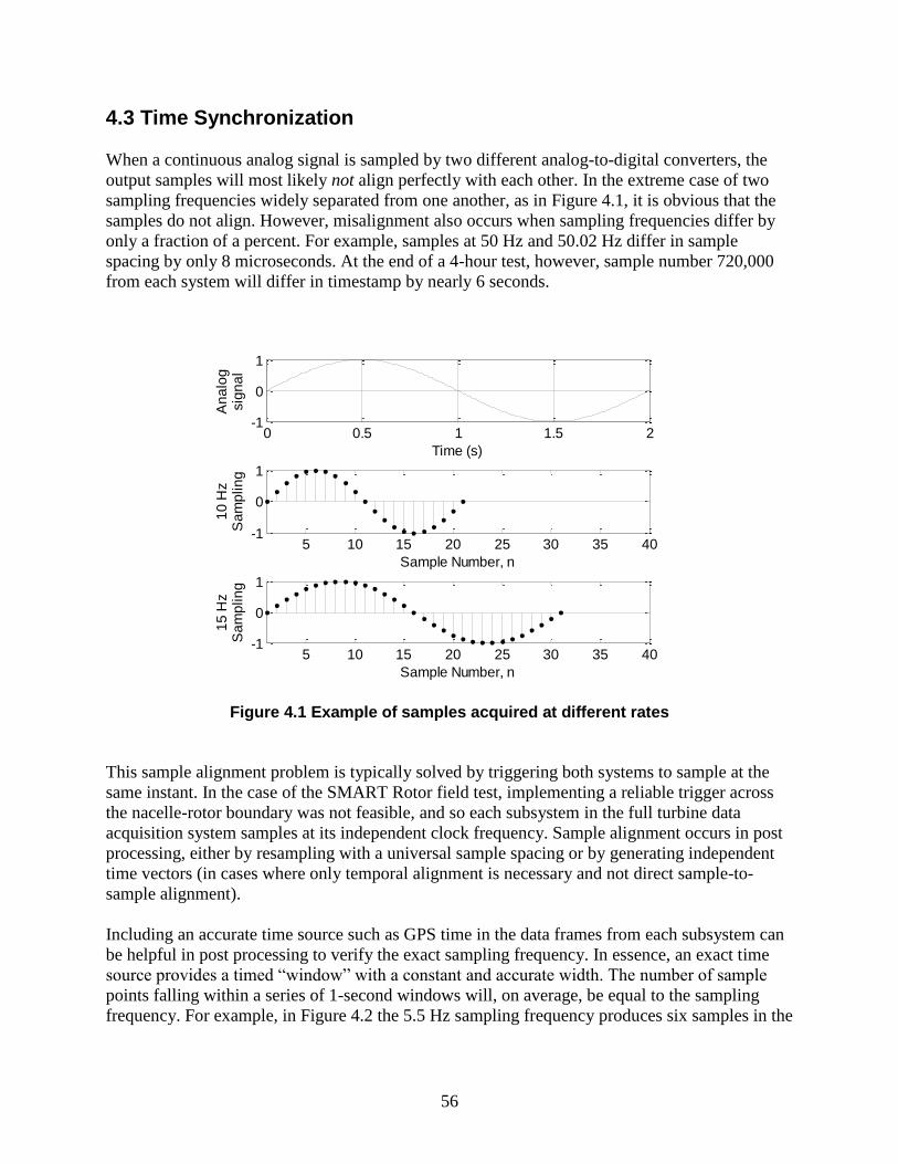
56
4.3 Time Synchronization
When a continuous analog signal is sampled by two different analog-to-digital converters, the
output samples will most likely not align perfectly with each other. In the extreme case of two
sampling frequencies widely separated from one another, as in Figure 4.1, it is obvious that the
samples do not align. However, misalignment also occurs when sampling frequencies differ by
only a fraction of a percent. For example, samples at 50 Hz and 50.02 Hz differ in sample
spacing by only 8 microseconds. At the end of a 4-hour test, however, sample number 720,000
from each system will differ in timestamp by nearly 6 seconds.
Figure 4.1 Example of samples acquired at different rates
This sample alignment problem is typically solved by triggering both systems to sample at the
same instant. In the case of the SMART Rotor field test, implementing a reliable trigger across
the nacelle-rotor boundary was not feasible, and so each subsystem in the full turbine data
acquisition system samples at its independent clock frequency. Sample alignment occurs in post
processing, either by resampling with a universal sample spacing or by generating independent
time vectors (in cases where only temporal alignment is necessary and not direct sample-to-
sample alignment).
Including an accurate time source such as GPS time in the data frames from each subsystem can
be helpful in post processing to verify the exact sampling frequency. In essence, an exact time
source provides a timed “window” with a constant and accurate width. The number of sample
points falling within a series of 1-second windows will, on average, be equal to the sampling
frequency. For example, in Figure 4.2 the 5.5 Hz sampling frequency produces six samples in the
0 0.5 1 1.5 2-1
0
1
An
alo
gsig
na
l
Time (s)
5 10 15 20 25 30 35 40-1
0
1
10
Hz
Sa
mp
lin
g
Sample Number, n
5 10 15 20 25 30 35 40-1
0
1
15
Hz
Sa
mp
lin
g
Sample Number, n

57
interval [0, 1) and five samples in the interval [1, 2)1. This 6-5 pattern repeats, and the long-term
average is 5.5 samples per second. If the number of windows happens to match the repeating
pattern then the answer will be exact. Otherwise, the number of samples included in the average
must be great enough that cutting the repeating pattern before the end does not significantly
change the average.
Figure 4.2 Example for sample rate determination
Instead of counting samples inside 1-second windows, it is likely more efficient to take the
following approach. Given a series of samples, their GPS time stamps are converted into the
number of seconds since the first sample. Plotting this array of time values against the sample
number of each sample gives a line with a slope which corresponds to the sample period
measured in seconds per sample. The line will have a stair-step appearance because the GPS time
does not update with every sample. However, a least-square fit of a straight line will easily
identify the slope which characterizes the stair-step.
After the sample period of each subsystem has been identified, it is possible to resample every
data channel so that they have a common sample rate. This eliminates the sample drift caused by
unequal sample spacing; however, the signals must still be synchronized in time.
GPS time is not very useful for temporal alignment of two signals because the update rate is
typically 1 Hz and every sample receives the same timestamp until another GPS update occurs.
To be useful for temporal alignment, the subsystem clocks need to be continually resynchronized
to GPS time and sampling must begin at a known instant in time which is consistent across all
subsystems.
In the absence of such a system directly controlled by GPS time, the sample clocks must be re-
aligned using features within the data itself. This is why certain signals were measured by both
the ACRA and cRIO. Calculating the cross-correlation of these signals identifies the amount of
time shift required to maximize the agreement between the signals.
1 The square bracket “[“ is used to indicate that a sample at the interval boundary would be included in the interval
and parenthesis “)” to indicate the sample would not be included.
0 0.5 1 1.5 2 2.5 3 3.5 4
Time (s)
5.5
Hz
Sam
plin
g

58
4.4 Data Dropouts
Data dropouts, or the occasional loss of a frame of data, were experienced in the field test. In
expectation of this possibility, the GBU, ACRA, and cRIO each created a “sequential frame ID”
or SFID which was packaged with the data frames. The SFID was a counter which incremented
every time the hardware acquired a frame of data. It was incremented whether or not the data
was successfully transmitted back to the host computer running ATLAS. Thus, it is possible to
detect data dropouts by looking for gaps in the SFID channels.
The GBU and ACRA subsystems generated 16-bit SFID values which range in value from 0 to
65535 and wrap around back to 0 after reaching the maximum value. The cRIO appears to
generate a 32-bit SFID value, which would mean a maximum value of around 4.29 billion, but
the SFID channel was never observed approaching the maximum and wrapping back to 0. When
detecting dropouts, the algorithm must take into account the maximum SFID value for each
subsystem and detect any data loss when the SFID wraps back to 0.
It was discovered after the field test that the cRIO’s SFID channel did not increment quite as
expected. Instead, the same value would be repeated in groups and the groups would occur in
patterns. The primary pattern was a group of three followed by a group of five which then
repeats, such as:
2, 2, 2, 6, 6, 6, 6, 6, 10, 10, 10, 14, 14, 14, 14, 14, …
In this example the sequence should have been the numbers 1 through 16. As written above, the
middle number in each group of three or group of five matches the true SFID. Numbers to the
right or left of the middle of a group need to be incremented or decremented by their distance
from the middle. It is not important to understand how this correction was applied to the cRIO’s
SFID channel but rather that a correction needed to be made in post processing. It is not clear
why the cRIO generated this pattern and in fact other patterns have been observed:
1, 3, 3, 3, 5, 7, 7, 7, 9, 10, 10, 10, … (a group of one, then three, repeating)
4 (seven times), 12 (nine times), 20 (seven times), …
For the most part, the cRIO did not have any data dropouts, in which case it was straightforward
to correct for the patterns observed. However, when a dropout did occur it disrupted the pattern
and made it difficult to automatically correct the SFID channel because it was impossible to
know which one of the repeated numbers in a pattern group was the one that had been dropped.
Therefore, when a disruption in the pattern was detected the SFID correction procedure was
stopped and the rest of the data from that point on was ignored.
The GBU averaged about 13 dropouts per ten-minute file. The RBU averaged about 45 dropouts
per ten-minute file. (A ten-minute file captured at 50 Hz contains 30,000 data frames.)

59
5. DATA POST PROCESSING
5.1 Scale and Offset
The scale and offset of a few data channels needed to be adjusted for various reasons outlined
below. Table 4.1 lists the values of the offsets and multipliers.
Channel 22, AZIMUTH_ANGLE, had an error in its channel configuration and needed to
be multiplied by 2.
Channel 32, LSS_SPEED, had an error in its channel configuration and needed to be
divided by 10.
Motor_Position channels (75, 77, 79, 81, 83, 85, 87, 89, 91) were output and recorded as
a 0-10 volt signals which needed to be converted to motor shaft angle in degrees.
Motor_Current channels (76, 78, 80, 82, 84, 86, 88, 90, 92) were output and recorded as a
0-10 volt signals which needed to be converted to current in amps.
Athena_AnalogOut channels (93, 94, 95) were output as a 0-5 volt signals and recorded
as a 0-10 volt signals which needed to be converted to commanded flap angle in degrees.
Certain accelerometer channels needed to be swapped in specific data files (which were
acquired prior to the time when the cable swap was corrected). Affected files include
those acquired before 16-Feb-2012 and those acquired on 5-Apr-2012.
DAQ_IMU_*_cRIO channels (147, 148, 149) needed to be converted from volts to
acceleration (g). The multiplier and offsets were obtained from the IMU calibration
report.
Channels 140 through 146 needed to be converted from volts to microstrain. The
multiplier and offsets were chosen to match the corresponding ACRA channels. Because
the ACRA strain offsets were observed to drift, the offsets were chosen to match data
from 24-Apr-2012 and 10-May-2012 which represent a major portion of the most useful
operational data.
It is important to note that the offsets for all foil strain gage measurements were observed to drift
over the duration of the field test. Thus the absolute magnitude of these strains is not directly
available. However the relative changes in strain during a particular test day can be utilized
because the drift can be assumed negligible over short time periods.

60
Table 5.1 Summary of post-processing offsets and multipliers applied according to Result = (Signal + Offset) x Multiplier
Offset Multiplier
LSS_SPEED 0
AZIMUTH_ANGLE 0 2
Motor_Position -5 (
)
Motor_Current -5
Athena_Analog -2.5
DAQ_IMU_X_cRIO -2.506 0.987
DAQ_IMU_Y_cRIO -2.509 1.005
DAQ_IMU_Z_cRIO -2.471 0.990
140 - B1_H1_Strain_0350_Z_HP 0* 91000
141 - B1_H1_Strain_0350_Z_LP 0.00062 91000
142 - B1_H1_Strain_2250_Z_HP -0.20* 91000
143 - B1_H1_Strain_4500_Z_HP -0.00380 91000
144 - B1_H1_Strain_6750_Z_HP -0.00018 91000
145 - B1_H1_Strain_0350_Z_TE -0.01* 91000
146 - B1_H1_Strain_0350_Z_LE -0.00012 91000
* - corresponding ACRA channel was not working

61
5.2 Coordinate Systems and Transformations
The accelerometers were mounted to the internal blade structure using angled mounting blocks
so that their axes of measurement would be roughly orthogonal with the desired blade coordinate
axes. However, the tri-axial accelerometers were rotated in 90 degree increments to
accommodate the ideal mounting orientation. In post-processing the channels were re-mapped to
obtain the desired blade coordinates.
Figure 5.1 illustrates the orientation of each accelerometer with respect to the blade coordinate
system and Table 5.2 provides the channel mapping into the blade coordinate system.
Figure 5.1 Orientation of accelerometers with respect to the blade coordinate system.
Table 5.2 Mapping of accelerometer channels to blade coordinate system
Original Accelerometer
Channel
New Accelerometer
Channel
Sign multiplier
Accel_2000_X_HP Accel_2000_ZB_HP -1
Accel_2000_Y_HP Accel_2000_XB_HP +1
Accel_2000_Z_HP Accel_2000_YB_HP -1
Accel_2000_X_TE Accel_2000_XB_TE +1
Accel_8000_X_HP Accel_8000_ZB_HP -1
Accel_8000_Y_HP Accel_8000_YB_HP +1
Accel_8000_Z_HP Accel_8000_XB_HP +1
Accel_8000_X_TE Accel_8000_XB_TE +1
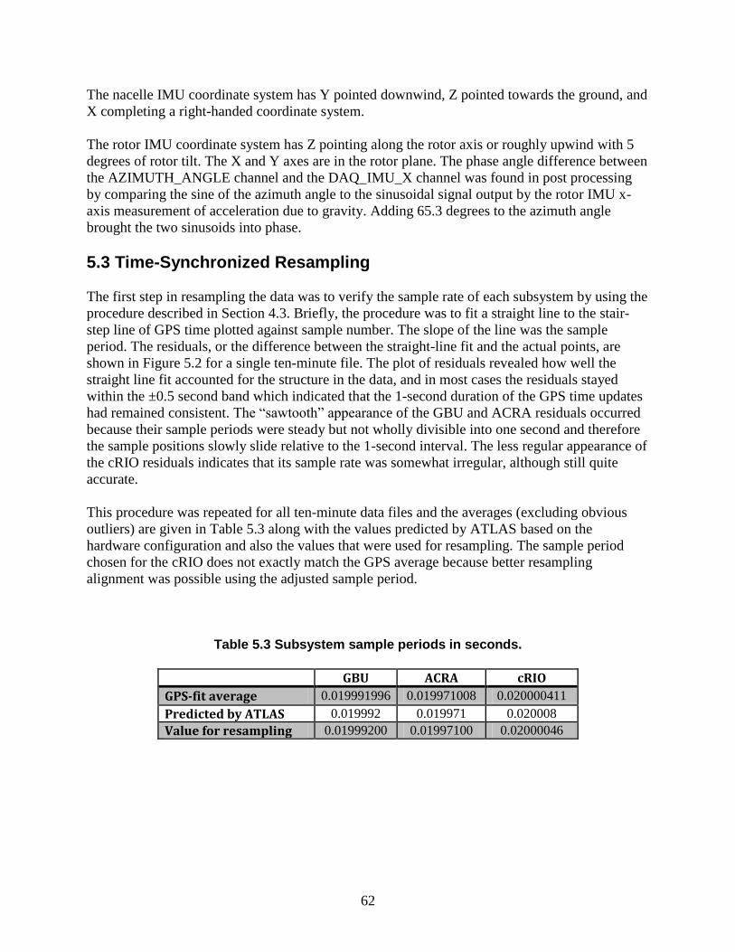
62
The nacelle IMU coordinate system has Y pointed downwind, Z pointed towards the ground, and
X completing a right-handed coordinate system.
The rotor IMU coordinate system has Z pointing along the rotor axis or roughly upwind with 5
degrees of rotor tilt. The X and Y axes are in the rotor plane. The phase angle difference between
the AZIMUTH_ANGLE channel and the DAQ_IMU_X channel was found in post processing
by comparing the sine of the azimuth angle to the sinusoidal signal output by the rotor IMU x-
axis measurement of acceleration due to gravity. Adding 65.3 degrees to the azimuth angle
brought the two sinusoids into phase.
5.3 Time-Synchronized Resampling
The first step in resampling the data was to verify the sample rate of each subsystem by using the
procedure described in Section 4.3. Briefly, the procedure was to fit a straight line to the stair-
step line of GPS time plotted against sample number. The slope of the line was the sample
period. The residuals, or the difference between the straight-line fit and the actual points, are
shown in Figure 5.2 for a single ten-minute file. The plot of residuals revealed how well the
straight line fit accounted for the structure in the data, and in most cases the residuals stayed
within the ±0.5 second band which indicated that the 1-second duration of the GPS time updates
had remained consistent. The “sawtooth” appearance of the GBU and ACRA residuals occurred
because their sample periods were steady but not wholly divisible into one second and therefore
the sample positions slowly slide relative to the 1-second interval. The less regular appearance of
the cRIO residuals indicates that its sample rate was somewhat irregular, although still quite
accurate.
This procedure was repeated for all ten-minute data files and the averages (excluding obvious
outliers) are given in Table 5.3 along with the values predicted by ATLAS based on the
hardware configuration and also the values that were used for resampling. The sample period
chosen for the cRIO does not exactly match the GPS average because better resampling
alignment was possible using the adjusted sample period.
Table 5.3 Subsystem sample periods in seconds.
GBU ACRA cRIO
GPS-fit average 0.019991996 0.019971008 0.020000411
Predicted by ATLAS 0.019992 0.019971 0.020008
Value for resampling 0.01999200 0.01997100 0.02000046

63
Figure 5.2 Pattern of residuals about straight-line fit to GPS time.
The next steps in resampling and aligning the data were to up-sample from the approximate 50
Hz sample rate to a common rate of 5000 Hz and then determine the amount of sample offset
between the alignment channels (see Section 4.2). Resampling to this higher frequency improved
the alignment resolution from 20 milliseconds to 0.2 milliseconds.
Resampling was accomplished with a frequency-domain technique described by Stearns and
Hush [56] which is also equivalent to the “resample” command in the MATLAB©
Signal
Processing Toolbox™ [57]. Being a frequency-domain technique, care was taken to ensure the
Nyquist-Shannon sampling theorem was satisfied. All channels, except the azimuth signal (22),
were acquired with an input low-pass filter of at least one-half the sample rate and in most cases
one-fourth the sample rate. One caveat was the data dropouts which needed to be filled in.
Although there are techniques for resampling irregular-spaced samples, numerical issues were
encountered when trying to apply them. So spline interpolation was used instead for data
dropouts with the assumption that the sampling theorem would still be satisfied during
resampling.
The azimuth signal was unique because it regularly “jumped” from 360 degrees to 0 degrees
which looked like a high frequency event. This was why a low-pass filter was not used on the
azimuth signal. Physically, however, the azimuth signal cannot have significant high frequency
content due to the rotor inertia, and so it was assumed that the sampling theorem was satisfied.
Resampling of the azimuth signal involved the following steps:
1. Transform the discontinuous signal into two continuous signals using sine and cosine
functions
2. De-spike the two transformed signals (the azimuth sensor did not always produce clean
output)
3. Resample both signals

64
4. Recombine the two signals using the inverse tangent function
The amount of time delay required for alignment was determined by calculating the cross-
correlation between alignment channels. Figure 5.3 diagrams the relationship of clock delays
between subsystems and channel offsets within subsystems.
Figure 5.3 Schematic of subsystem clock delays and channel offsets
The beginning of the cRIO’s data stream always occurred later in time than those of the ACRA
and the GBU data streams. The result was that beginning segments of ACRA and GBU channels
had to be discarded so that all of the first samples were in alignment. Because the cRIO’s first
data frame became the first one in the resampled data, it was convenient to reference the clock
delays to Clock 1 (the cRIO).
The clock delays between subsystems changed every time a new data acquisition session began.
These variable delays likely resulted from network communication lags and differences in
system start-up time when ATLAS instructed each subsystem to begin acquiring data.
The channel offsets within each subsystem were constant and resulted from differences in input
filter configuration or module function. These fixed channel offsets were verified with post-test
measurements acquired with a common voltage signal routed to all sensor channels. Table 5.4
lists the measured offsets. Motor channels (75..92) were slightly different than the rest because
extra hardware was required to obtain and convert these signals which produced offsets in
addition to the inherent ACRA delays. The expected offsets for the motor channels are given but
have not been directly verified.
The final step in resampling was to down-sample to 50 Hz by simple decimation (discarding data
points).
cRIO (107..186) Clock 1
ACRA (87..101) Clock 2 delay
GBU (22) Clock 3 delay
ACRA (48..86) Channel offset
GBU (6..21, 23..38) Channel offset

65
Table 5.4 Channel offsets relative to subsystem clocks measured in number of samples at 5 kHz resampling
Channels Clock ID
Channel offset (samples at 5 kHz)
22 3 0
6..21, 23..32, 35..38 3 5256
33..34 3 5275
48..74 2 3395
75, 81 2 3395 + 55
76, 82 2 3395 + 45
77, 83 2 3395 + 35
78, 84 2 3395 + 25
79, 85 2 3395 + 15
80, 86 2 3395 + 5
87 2 55
88 2 45
89 2 35
90 2 25
91 2 15
92 2 5
93..101 2 0

66

67
6. ON-GROUND CALIBRATION
ATA Engineering was contracted to assist with the blade modal test and analysis. The following
sections are preliminary results of the modal characterization and model updating tasks. These
results were calculated before the time synchronization issues were fully understood, but they
should still be valid because the cRIO’s signals were the focus of the modal analysis.
A subsequent update to these preliminary results was planned for the purpose of creating a well-
tuned turbine model appropriate for closed-loop control design. However, with the project test
window being cut short and the Bushland Test Site subsequently decommissioned, the final
update was no longer a high priority.
The on-ground testing included impact test data while each of the blades was suspended using
metal cables to mimic a free-free boundary condition as well as when the blade was cantilevered
off of a fixed hub. Static pull testing in both the edge and flap directions was also performed
when the blade was in the cantilevered configuration.
ATA Engineering’s analysis utilized only the modal impact data acquired while the blade was in
the free-free boundary condition for the initial modal characterization of the SMART blades and
the model updating procedure. This subset of the data was selected because it was believed that
assumption of the free-free boundary condition in the suspended configuration was more
accurate than the assumption of the cantilever boundary condition when the blade was attached
to the hub due to the residual rotational flexibility of the hub.
6.1 Preliminary Blade Modal Properties
To experimentally determine the modal properties of the SMART blades, each of the blades was
excited using an instrumented modal impact hammer at nine different locations on each blade.
The relatively small number of impact locations was due to the limited amount of time for testing
and the fact that 60 seconds were needed to capture the response of the structure after each
impact. Due to the sparse nature of the impact locations a simple beam model of the blade was
used for displaying the mode shapes and is shown in Figure 6.1. At locations 21, 22, and 25
through 29 the blades were impacted in both the flap and edge directions. Rigid body
completion was used to determine the Y-direction deformations of nodes 23 and 24. No axial
deformations (in the Z-direction) were considered in this analysis.
A batch processing methodology was developed to ease future analyses of similar data sets. The
data from each of the data files generated by ATLAS were unzipped and loaded into Matlab and
the associated header files were parsed to obtain the pertinent information. These files were then
concatenated so that a single set of time data was created for each test. Then the associated
Excel modal test log was open and parsed using Matlab to determine the node number and
direction of each impact on the blade.

68
Figure 6.1 Simple beam element model used to display the experimental mode shapes.
The time histories were then converted into Frequency Response Functions (FRFs) using ATA’s
spFRF signal processing tool which calculated the average auto- and cross- spectral densities of
the Impact Hammer and all eight response accelerometers for each of the impact locations.
These auto- and cross-spectra were then used to estimate the systems FRFs using the H1
estimator.
After the FRF matrix had been created using all 8 accelerometers and all 19 impact coordinates
the systems natural frequencies and damping values were estimated using the alias-free
polyreference algorithm. The alias-free polyreference technique, in ATA’s AFPoly™ IMAT
toolkit, employs a Laplace-domain, curve-fitting algorithm. Damping was estimated using the
same polyreference FRF curve-fitting algorithm that was used to extract the resonant
frequencies. The mode shapes were then calculated by refitting the FRFs using the extracted
system poles and rigid body completion was used to estimate the deformation of the unmeasured
degrees-of-freedom for visualization purposes.
Further investigation of the modal impact data revealed that rotation of the blades during testing
caused a perturbation of the mode shapes and natural frequencies due to the varying stiffness of
the boundary conditions. One way in which this is evident is through the shift in the resonant
frequencies of the blade depending on the blade’s orientation. For instance when the trailing
edge of the Blade 3 was pointing upwards (as in Figure 5.1) the resonant frequency of the first
flap bending mode was approximately 7.3 Hz and the second bending mode occurred at
approximately 17.7 Hz. However, when Blade 3 was rotated so that its chord line was
approximately horizontal these modes appeared to shift to approximately 7.5 and 20.3 Hz.
In an attempt to minimize the influence of this rotation on the extracted modal parameters, the
poles of the system were extracted from the impacts and response measurements that were
perpendicular to the direction of gravity (parallel to the weak axis of the supports). This means
that the modal frequency and damping values were calculated using only the measurements from
when the structure was closest to free-free in that direction for each mode. The calculated poles
were then used to estimate the mode shapes using the impacts in both directions. However,
because of the physical change in the system this means that the estimates of the mode shapes in
the non-dominant direction of motion (edge-wise for flap bending modes and vice-versa) are
likely much less accurate than the calculated mode shapes in the dominant direction of motion.
Therefore, ATA recommended that in future testing the metal cables be replaced with bungees
and that at least one of the blades be impacted in both directions for both configurations. Metal

69
cables were used in this test to avoid adding extra damping. An alternative approach may be to
loop the blade using the metal cable and then connect these loops to the support truss through
intermediate bungees. In this way the material in contact with the structure remains the same
while the stiffness of the support system would be significantly reduced. If the boundary
condition remains too stiff in the vertical direction it could also be modeled as grounded springs
during the correlation process as long as impacts in both directions are obtained while the blade
is in a single configuration.
Using the directional method described above to estimate the natural frequencies and damping
values of all three of the blades, the values in Table 6.1 were calculated using the previously
described Alias-Free Polyreference algorithm. The modal properties of the blades are relatively
consistent with the standard deviation of the natural frequencies of the blades for the flexible
modes all being less than 2.1% of the average natural frequency. In fact, other than the second
flap bending edge bending mode, the standard deviation of the natural frequencies varied by less
than 1% of the average for each mode.
Table 6.1 Free-free natural frequency and damping values for all three of the SMART blades. Five flexible modes were calculated in addition to three rigid body modes.
6.2 Preliminary Beam Model Updating
Initial beam model parameters were calculated from an ANSYS blade model using BPE. The
mass densities per unit length that were calculated using BPE were left consistent but the mass
densities were scaled so that the total mass of the blade was scaled to match the experimental
average of the CX-100 blades. In order to account for the added mass of the lightning protection
in the SMART blades a total of 5 kg was added evenly along the blade by increasing each of the
mass densities accordingly. The planned final update to these analyses would have also included
the change in mass distribution due to the addition of the flap modules.
For the correlation procedure only the edge- and flap-wise distributed stiffness values were
modified. In order to update this model while maintaining realistic stiffness parameters
constrained minimization was performed. Because both the distributed stiffness parameters of
the beam were to be updated both the natural frequencies and the mode shapes of the model
needed to be compared. Consequently, the optimization function was calculated using a
weighted sum of the RMS of the differences in the natural frequencies and the RMS of one
minus the modal assurance criteria calculated between the corresponding mode shape for the
model and the experimental results (commonly referred to as the Cross-MAC). However, due to
the difficulty in estimating the mode shapes in the non-dominant direction (edge-wise motion for
Mode Mode Shape
Number Freq (Hz) Damp (% Cr) Freq (Hz) Damp (% Cr) Freq (Hz) Damp (% Cr) Freq (Hz) Damp (% Cr) Description
RB1 0.25 6.0 0.26 5.8 0.26 5.9 0.26 5.93 Rigid Body Horizontal Twist (about Y-Axis)
RB2 0.31 3.9 0.29 4.8 0.33 3.5 0.31 4.07 Rigid Body Vertical Twist (about X-Axis)
RB3 2.69 1.0 2.62 1.4 2.61 0.6 2.64 1.02 Rigid Body Longitudinal Twist (about Z-Axis)
1 7.28 0.5 7.19 0.5 7.21 0.6 7.23 0.53 First Flap Bending
2 15.91 1.1 15.63 1.0 15.74 1.2 15.76 1.12 First Edge Bending
3 17.92 1.0 17.57 0.9 17.73 1.0 17.74 0.96 Second Flap Bending
4 29.27 1.5 29.21 1.1 29.52 0.9 29.33 1.15 Third Flap Bending
5 36.68 1.5 35.93 1.7 37.44 0.4 36.68 1.22 Second Edge Bending
Blade 1 Blade 2 Blade 3 Average

70
flap dominant modes) mentioned above, the Cross-MAC was only calculated in the dominant
direction of motion (only flap deflections were used for modes that were dominant in the flap
direction).
Table 5.2 shows a comparison of the percent errors in the natural frequencies as well as the MAC
values for each of the three different correlated models. As can be seen, a high degree of
correlation was obtained for each of the three blades. The change in the stiffness values for each
of the beam elements was then investigated and the changes in the flap-wise and edge-wise
stiffness values along the length of the beam can be seen in Table 5.3 and Table 5.4 respectively.
For both sets of stiffness values, by far the largest percent changes occurred near the tip of the
blade. This was anticipated due to the changes in the SMART blade layup; however, these
results would change somewhat if the flap module masses were fully accounted.
Table 6.2 Comparison of the free-free experimental results for each blade as well as the
model correlated to each blade.
Table 6.3 Flapwise stiffness along the length of the blade (Bld Fract) calculated directly
from BPE (Uncorrelated) and using each of the correlated models. The average stiffness values and the percent change between the average value and the initial value are also
shown.
Mode Uncorrelated
Number Nat. Freq. (Hz) Exp. (Hz) Model (Hz) % Err MAC Exp. (Hz) Model (Hz) % Err MAC Exp. (Hz) Model (Hz) % Err MAC
1 7.08 7.28 7.28 0.0% 99.8% 7.19 7.19 0.0% 99.7% 7.21 7.22 -0.1% 99.7%
2 14.04 15.91 15.91 0.0% 98.7% 15.63 15.41 1.5% 97.7% 15.74 15.12 4.0% 97.9%
3 16.77 17.92 17.92 0.0% 99.8% 17.57 17.59 -0.1% 99.9% 17.73 17.76 -0.1% 99.7%
4 30.54 29.27 29.27 0.0% 99.7% 29.21 29.21 0.0% 99.8% 29.52 29.54 -0.1% 99.9%
5 33.82 36.68 36.68 0.0% 98.2% 35.93 35.76 0.5% 95.7% 37.44 37.81 -1.0% 96.7%
Blade 2 Results Blade 3 ResultsBlade 1 Results
Bld Fract Uncorrelated Blade 1 Blade 2 Blade 3 Average Ave % Change
1.4% 3.62E+07 3.62E+07 3.62E+07 3.62E+07 3.62E+07 0.01%
5.3% 1.16E+07 1.16E+07 1.16E+07 1.16E+07 1.16E+07 -0.03%
10.3% 3.99E+06 3.99E+06 3.98E+06 3.98E+06 3.98E+06 -0.04%
15.3% 3.48E+06 3.49E+06 3.48E+06 3.48E+06 3.48E+06 -0.04%
20.6% 2.92E+06 2.92E+06 2.91E+06 2.91E+06 2.92E+06 -0.12%
26.7% 2.19E+06 2.19E+06 2.19E+06 2.19E+06 2.19E+06 -0.09%
32.6% 1.52E+06 1.52E+06 1.52E+06 1.52E+06 1.52E+06 -0.08%
37.9% 1.06E+06 1.06E+06 1.06E+06 1.06E+06 1.06E+06 -0.10%
44.4% 6.82E+05 6.85E+05 6.82E+05 6.76E+05 6.81E+05 -0.15%
51.5% 4.19E+05 4.22E+05 4.18E+05 4.16E+05 4.19E+05 -0.03%
59.1% 2.40E+05 2.29E+05 2.22E+05 2.30E+05 2.27E+05 -5.60%
68.9% 1.07E+05 8.66E+04 8.30E+04 8.41E+04 8.46E+04 -20.85%
79.2% 3.51E+04 8.24E+04 1.00E+05 8.87E+04 9.05E+04 157.80%
87.5% 1.07E+04 1.60E+04 1.18E+04 1.22E+04 1.33E+04 24.62%
94.2% 2.25E+03 1.43E+03 1.58E+03 1.82E+03 1.61E+03 -28.38%
98.6% 4.17E+02 1.25E+03 1.24E+03 1.65E+02 8.85E+02 112.43%
Flap-wise Stiffness (N-m^2)

71
Table 6.4 Edgewise stiffness along the length of the blade (Bld Fract) calculated directly from BPE (Uncorrelated) and using each of the correlated models. The average stiffness values and the percent change between the average value and the initial value are also
shown.
The average stiffness values in both the flap and edge direction were then calculated using all
three models. The natural frequencies for this average model compared closely to the
experimental average natural frequency across the three SMART blades as can be seen in Table
5.5 as the largest percent error in the natural frequencies was less than 2.5%.
Table 6.5 Average free-free experimental natural frequencies and the natural frequencies
calculated from a beam model with the average stiffness values from each of the correlated models.
Bld Fract Uncorrelated Blade 1 Blade 2 Blade 3 Average Ave % Change
1.4% 4.19E+07 4.19E+07 4.19E+07 4.19E+07 4.19E+07 0.01%
5.3% 6.79E+06 6.79E+06 6.79E+06 6.79E+06 6.79E+06 0.04%
10.3% 1.96E+06 1.98E+06 1.97E+06 1.97E+06 1.97E+06 0.65%
15.3% 2.33E+06 2.36E+06 2.36E+06 2.34E+06 2.35E+06 0.82%
20.6% 3.56E+06 3.58E+06 3.57E+06 3.57E+06 3.57E+06 0.44%
26.7% 4.13E+06 4.16E+06 4.14E+06 4.13E+06 4.14E+06 0.35%
32.6% 3.52E+06 3.55E+06 3.54E+06 3.52E+06 3.54E+06 0.49%
37.9% 2.75E+06 2.81E+06 2.78E+06 2.76E+06 2.78E+06 1.08%
44.4% 2.04E+06 2.14E+06 2.09E+06 2.05E+06 2.09E+06 2.78%
51.5% 1.41E+06 1.54E+06 1.48E+06 1.42E+06 1.48E+06 5.17%
59.1% 9.05E+05 1.16E+06 1.03E+06 9.44E+05 1.04E+06 15.40%
68.9% 4.78E+05 9.34E+05 7.72E+05 6.41E+05 7.82E+05 63.64%
79.2% 2.06E+05 6.19E+05 6.19E+05 5.32E+05 5.90E+05 185.91%
87.5% 8.54E+04 7.02E+04 6.29E+04 1.82E+05 1.05E+05 22.85%
94.2% 3.02E+04 9.96E+03 9.96E+03 9.96E+03 9.96E+03 -67.00%
98.6% 1.11E+04 3.67E+03 3.67E+03 3.67E+03 3.67E+03 -66.99%
Edge-wise Stiffness (N-m^2)
Mode Average Ave Model Percent
Number Nat. Freq. (Hz) Nat. Freq. (Hz) Error (%)
1 7.23 7.24 -0.14%
2 15.76 15.56 1.27%
3 17.74 17.84 -0.58%
4 29.33 29.47 -0.47%
5 36.68 37.58 -2.45%

72
6.3 Blade Strain Calibrations
Static pull testing in both the edge and flap directions was performed when the blade was in the
cantilevered configuration. The blade root was bolted to a calibration fixture with the blade
leading edge down and cantilevered parallel to the ground. The calibration fixture itself was a
Micon 65/13 hub which had been attached to a support structure that also acted as a pull frame.
A strain gage shunt calibration was performed first to zero the completion bridges and record the
baseline strain values. The blade was then loaded in the both the edgewise and flapwise
directions in six load steps up to 300 pounds-force. Flapwise loading was applied just inboard of
the active control modules at 7 m span and edgewise loading was applied at 7.2 m span.
Displacement measurements along the blade were obtained from a laser displacement transducer
and string displacement potentiometers. Figure 6.2 is a photo of the edgewise blade pull.
Table 6.6 contains the resulting strain calibration slopes and intercepts.
Table 6.6 Blade strain calibration. Measurement units for
slope and intercept are (microstrain / lbf) and (microstrain), respectively.
Flap Pull Edge Pull
slope intercept slope intercept
B1_H1_Strain_0350_Z_HP 0.0808 2.5114 -0.0122 -0.8714
B1_H1_Strain_0350_Z_LP -0.0585 -1.9117 -0.0135 -1.1559
B1_H1_Strain_2250_Z_LP -0.3285 -15.025 0.1358 -5.2972
B1_H1_Strain_4500_Z_LP -0.6236 -23.779 0.1701 -4.4313
B1_H1_Strain_6750_Z_LP -0.1784 -5.9871 0.0537 1.639
B1_H1_Strain_0350_Z_TE -0.0043 4.5315 -0.1115 2.3311
B1_H1_Strain_0350_Z_LE -0.0244 -9.5567 0.1409 -6.8395
B2_H2_Strain_0350_Z_HP 0.0678 2.1348 -0.0163 0.4519
B2_H2_Strain_0350_Z_LP -0.0630 -1.9036 -0.0173 -1.7284
B2_H2_Strain_2250_Z_LP -0.2967 -5.4967 0.1465 2.4077
B2_H2_Strain_4500_Z_LP -0.5870 -15.541 0.1914 0.5457
B2_H2_Strain_6750_Z_LP -0.1847 -9.3699 0.0683 -5.2529
B2_H2_Strain_0350_Z_TE
B2_H2_Strain_0350_Z_LE -0.0081 -6.7704 0.0738 -6.0823
B3_H3_Strain_0350_Z_HP 0.0532 -0.1968 -0.0102 -0.8004
B3_H3_Strain_0350_Z_LP -0.0708 3.3771 -0.0084 -1.0359
B3_H3_Strain_2250_Z_LP -0.3145 -29.356 0.171 -15.489
B3_H3_Strain_4500_Z_LP -0.6658 -36.96 0.2568 -13.8
B3_H3_Strain_6750_Z_LP -0.1794 -7.7114 0.1034 -1.1667
B3_H3_Strain_0350_Z_TE
B3_H3_Strain_0350_Z_LE 0.0049 4.2217 0.0926 6.42
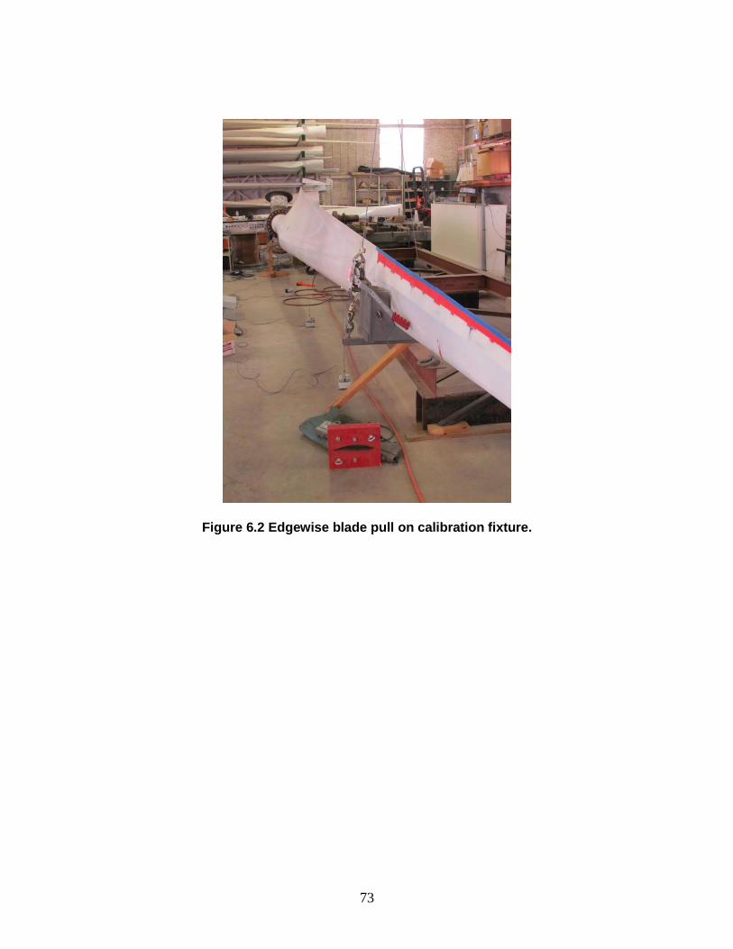
73
Figure 6.2 Edgewise blade pull on calibration fixture.

74

75
7. BLADE SURFACE GEOMETRY
The reduction in power output of the SMART rotor compared to a previous CX-100 field test
(see Section 3.5) prompted an investigation into possible causes. One possibility was a difference
in blade surface geometry. When the SMART rotor was built, the flap modules were designed
and manufactured in parallel with the blades themselves. As a result, the flap modules, which
were based on the geometry of an existing CX-100 blade tip, did not exactly match the geometry
of the SMART blades. The mismatch was smoothed over with a flexible filler material.
To acquire a scan of the entire surface geometry, Creaform [58] was contracted to use one of
their handheld optical scanning systems. Creaform chose to utilize their “MetraSCAN 3D”
system, which is a combination of a handheld optical scanner and a stereo camera that locates the
scanner in three-dimensional space. Figure 7.1 shows the scanning system and one SMART
blade with optical targets scattered along the surface. Figure 7.2 is the resulting “point cloud” for
one blade.
Figure 7.1 Creaform used their handheld optical scanning system to scan each blade.
Figure 7.2 The entire surface of each blade was scanned,
resulting in a high density “point cloud”.

76
Figure 7.3 Detail of a SMART blade tip with flaps positioned at -20 degrees.
Figure 7.3 shows some of the detail captured at the tip of one SMART blade with the flaps
positioned at -20 degrees. The five patches or voids are locations where an optical target was
attached. The high density of points captured many of the surface geometry details that could
perturb the air flow.
The entire blade surface was scanned so that the chord and twist distributions could be found and
the exact location of any cross section would be known relative to the root. In addition to scans
of the three SMART blades, a standard CX-100 blade was scanned.
Figure 7.4 compares the chord distributions of SMART Blade #2, the sample CX-100 blade, and
the available CX-100 design information. The chord distributions of the two scans matched very
well. The design chord distribution was off in the root transition region and the last half meter of
the tip, which was expected because these areas of the blade mold were constructed “free-form”
by hand and not measured until now.
Figure 7.5 compares the twist distributions of SMART Blade #2, the sample CX-100 blade, and
the available CX-100 design information. The twist offsets of the two scans were adjusted to
align their overall distributions with the design data. Also note that the measured twist
distributions are somewhat noisy because identifying the chord line of a measured airfoil has
some error involved which is amplified when calculating the chord line angle. However, it
appears the sample CX-100 blade aligns well with the design data but the SMART blade has a
deviation in twist starting just outboard of 6 meter span which results in on offset of -1.4 degrees
at the tip.
This small change in twist distribution would tend to decrease power output but analysis
predicted that the effect was relatively small and occurred mostly at higher wind speeds as the
blade began to stall. The more significant geometry changes appear to be those which occurred
locally on the airfoil cross section shapes.

77
Figure 7.4 Chord distributions of SMART Blade #2, a CX-100 blade,
and the available CX-100 design information.
Figure 7.5 Twist distributions of SMART Blade #2, a CX-100 blade,
and the available CX-100 design information.

78
Although all of the blades were manufactured from the same mold, comparison of SMART
Blade #2 and the sample CX-100 blade reveal that the geometry matched almost exactly at some
cross sections but had significant variation at others. Figures 7.6 through 7.9 exemplify the
observed similarities and differences. Figures 7.8 and 7.9 illustrate how the geometry mismatch
was corrected when the flap modules were interfaced to the blades. Note that the modules were
thicker than the sample CX-100 blade, which indicates the blade tip on which the modules were
based was also different from the CX-100 shown here. A strip of precurved mylar plastic was
applied to the low-pressure surface of the blades along the flap hinge line. The plastic was
bulged outward during the blade scans but should have lain down somewhat during turbine
operation.
Figure 7.6 Cross sections at 3 meter span align almost perfectly.
Figure 7.7 Cross sections at 5 meter span show variation in thickness.

79
Figure 7.8 Cross sections at 7.2 meter span annotated with SMART blade alterations.
Figure 7.9 Cross sections at 7.9 meter span with variations annotated.
These cross section variations were likely contributors to the reduced power performance. The
variations also highlight the difficulty of integrating additional hardware into a manufacturing
process which can produce significant blade-to-blade variation.

80

81
8. REFERENCES
1. U.S. Department of Energy. “Report on the First Quadrennial Technology Review,” DOE/S-
0001, Washington, DC, September 2011.
2. U.S. Department of Energy. “20% Wind Energy by 2030,” DOE/GO102008-2567,
Washington, DC, July 2008.
3. T.K. Barlas and G.A.M. van Kuik. “Review of state of the art in smart rotor control research
for wind turbines,” Progress in Aerospace Science (2009),
doi:10.1016/j.paerosci.2009.08.002
4. J-W van Wingerden, A.W. Hulskapp, T. Barlas, B. Marrant, G.A.M. van Kuik, D-P
Molenaar, and M. Verhaegen, “On the Proof of Concept of a ‘Smart’ Wind Turbine Rotor
Blade for Load Alleviation”, Wind Energy, 2008; 11:265-80.
5. T. Barlas, J-W van Wingerden, A. Hulskamp, and G. van Kuik, “Closed-loop Control Wind
Tunnel Tests on an Adaptive Wind Turbine Blade for Load Reduction,” Proceedings of the
46th AIAA/ASME, Reno, NV, USA, 2008.
6. N. Troldborg, “Computational study of the Risø B1-18 airfoil with a hinged flap providing
variable trailing edge geometry.” Wind Engineering 2005, 29:89-113.
7. T. Buhl, M. Gaunaa, and C. Bak, “Load reduction potential using airfoils with variable
trailing edge geometry,” Proceedings of the 43th AIAA/ASME, Reno, NV, USA, 2005.
8. T. Buhl, M. Gaunaa, and C. Bak, “Potential load reduction using airfoils with variable
trailing edge geometry.” Solar Energy Engineering 2005, 127:503-16.
9. P. B. Andersen, M. Gaunaa, C. Bak, and T. Buhl, “Load alleviation on wind turbine blades
using variable airfoil geometry,” Proceedings of the EWEC 2006, Athens, Greece.
10. P. B. Andersen, M. Gaunaa, C. Bak, and T. Buhl, “Wind tunnel test on wind turbine airfoil
with adaptive trailing edge geometry,” Proceedings of the 45th AIAA/ASME, Reno, NV,
USA, 2007.
11. T. Buhl, “Stability Limits for a Full Wind Turbine Equipped with Trailing Edge Systems,”
European Wind Energy Conference, Marseille, France, 16-19 March, 2009.
12. P.B. Anderson, “Load Reduction Using Pressure Difference on Airfoil for Control of
Trailing Edge Flaps,” European Wind Energy Conference, Marseille, France, 16-19 March,
2009.
13. D.G. Wilson, D.E. Berg, M.F. Barone, J.C. Berg, B.R. Resor, and D.W. Lobitz, “Active
Aerodynamic Blade Control Design for Load Reduction on Large Wind Turbines,” European
Wind Energy Conference, Marseille, France, 26-19 March, 2009.

82
14. D.E. Berg, D.G. Wilson, M.F. Barone, J.C. Berg, B.R. Resor, J.A. Paquette, and J.R. Zayas,
“The Impact of Active Aerodynamic Load Control on Fatigue and Energy Capture at Low
Wind Speed Sites,” European Wind Energy Conference, Marseille, France, 16-19 March,
2009.
15. D.E. Berg, D.G. Wilson, B.R. Resor, M.F. Barone, J.C. Berg, S. Kota, and G. Ervin, “Active
Aerodynamic Blade Load Control Impacts on Utility-Scale Wind Turbines,” WINDPOWER
2009, Chicago, Illinois, 5-7 May, 2009.
16. D.G. Wilson, D.E. Berg, B.R. Resor, M.F. Barone, and J.C. Berg, “Combined Individual
Pitch Control and Active Aerodynamic Load Controller Investigation for the 5MW UpWind
Turbine”, WINDPOWER 2009, Chicago, Illinois, 5-7 May, 2009.
17. B. Resor, D. Wilson, D. Berg, J. Berg, T. Barlas, and G. van Kuik, “The Impact of Higher
Fidelity Models on Active Aerodynamic Load Control Fatigue Damage Reduction,”
Proceedings of the 48th AIAA Aerospace Sciences Meeting, Orlando, FL, January 4-7, 2010.
18. D.G. Wilson, B.R. Resor, D.E. Berg, T.K. Barlas, and G.A.M. van Kuik, “Active
Aerodynamic Blade Distributed Flap Control Design Procedure for Load Reduction on the
UpWind 5MW Wind Turbine,” Proceedings of the 48th AIAA Aerospace Sciences Meeting,
Orlando, FL, January 4-7, 2010.
19. D.E. Berg, D. Wilson, B. Resor, J. Berg, T. Barlas, A. Crowther, and C. Halse, “System ID
Modern Control Algorithms for Active Aerodynamic Load Control and Impact on Gearbox
Loading,” The Science of Making Torque from Wind, 2010.
20. J. Berg, B. Resor, J. Paquette, and J. White, “SMART Wind Turbine Rotor: Design and Field
Test.” SAND2014-0681, Sandia National Laboratories, Albuquerque, NM.
21. D. Castaignet, J.J. Wedel-Heinen, T. Kim, T. Buhl, and N.K. Poulsen, “Results from the first
full scale wind turbine equipped with trailing edge flaps.” (AIAA 2010-4407, Proceedings of
the 28th AIAA Applied Aerodynamics Conference, Chicago, Illinois, 28 June – 1 July 2010)
22. Damien Castaignet, Thanasis Barlas, Thomas Buhl, Niels K. Poulsen, Jens Jakob Wedel-
Heinen, Niels A. Olesen, Christian Bak, and Taeseong Kim, “Full-scale test of trailing edge
flaps on a Vestas V27 wind turbine: active load reduction and system identification.”
(Journal of Wind Energy, 2013, DOI: 10.1002/we.1589)
23. J. G. Leishman. “Challenges in modelling the unsteady aerodynamics of wind turbines.”
Wind Energy, 5:85–132, 2002.
24. L. J. Vermeer, J. N. Sørensen, and A. Crespo. “Wind turbine wake aerodynamics.” Progress
in Aerospace Sciences, pages 467–510, 2003.
25. M. Lackner and G. van Kuik. “A comparison of smart rotor control approaches using trailing
edge flaps and individual pitch control.” AIAA Paper 2009-685, 2009.

83
26. H. Snel. “Survey of induction dynamics modelling within BEM-like codes: Dynamic inflow
and yawed flow modelling revisited.” AIAA Paper 2001-0027, 2001.
27. M. Gaunaa. “Unsteady 2D potential-flow forces on a thin variable geometry airfoil
undergoing arbitrary motion.” Technical Report Risø-R-1478, Risø-DTU, 2004.
28. M. P. Kinzel, M. D. Maughmer, and G. A. Lesieutre. “Miniature trailing-edge effectors for
rotorcraft performance enhancement.” J. Am. Helicopter Soc., 52(2):146–158, 2007.
29. P. B. Andersen, M. Gaunaa, C. Bak, and M. H. Hansen. “Implementing a dynamic stall
model for airfoils with deformable trailing edges.” AIAA Paper 2008-1328, 2008.
30. S. Schreck and M. Robinson. “Boundary layer state and flow field structure underlying
rotational augmentation of blade aerodynamic response.” J. Solar Energy Engineering –
Transactions of the ASME, 125(4):448–456, 2003.
31. H. Glauert. Airplane propellers. In W. F. Durand, editor, Aerodynamic Theory. Julius
Springer, Berlin, Germany, 1935.
32. D. M. Pitt and D. A. Peters. “Theoretical prediction of dynamic-inflow derivatives.” Vertica,
5(1):21–34, 1981.
33. D. A. Peters, D. D. Boyd, and C. J. He. “Finite-state induced-flow model for rotors in hover
and forward flight.” J. American Helicopter Soc., 34(4):5–17, 1989.
34. C. J. He. Development and application of a generalized dynamic wake theory for lifting
rotors. PhD thesis, Georgia Institute of Technology, July 1989.
35. P. J. Moriarty and A. C. Hansen. AeroDyn Theory Manual. Technical Report NREL/EL-500-
36881, National Renewable Energy Laboratory, 2005.
36. M. Joglekar and R. Loewy. “An actuator-disc analysis of helicopter wake geometry and the
corresponding blade response.” USAAVLABS Technical Report 69-66, 1970.
37. J. G. Leishman, M. J. Bhagwat, and A. Bagai. “Free-vortex filament methods for the analysis
of helicopter rotor wakes.” J. of Aircraft, 39(5):759–775, 2002.
38. S. G. Voutsinas, V. A. Riziotis, and P. Chaviaropoulos. “Non-linear aerodynamics and
fatigue loading on wind turbines operating at extreme sites.” AIAA Paper 97-0935, 1997.
39. S. Gupta and J. G. Leishman. “Comparison of momentum and vortex methods for the
aerodynamic analysis of wind turbines.” AIAA Paper 2005-594, 2005.
40. S. Gupta and J. G. Leishman. “Validation of a free-vortex wake model for wind turbines in
yawed flow.” AIAA Paper 2006-389, 2006.
41. S. Gupta and J. G. Leishman. “Performance predictions of the NREL Phase VI combined
experiment rotor using a free-vortex wake model.” AIAA Paper 2006-390, 2006.

84
42. T. Sant, G. van Kuik, and G. van Bussel. “Estimating the unsteady angle of attack from blade
pressure measurements on the NREL Phase VI rotor in yaw using a free-wake vortex
model.” AIAA Paper 2006-393, 2006.
43. S. Cline and C. Crawford. “Comparison of potential flow wake models for horizontal-axis
wind turbine rotors.” AIAA Paper 2010-463, 2010.
44. G. Xu and L. N. Sankar. “Computational study of horizontal axis wind turbines.” AIAA
Paper 99-0042, 1999.
45. C. P. van Dam, J. C. Vander Kam, and J. K. Paris. “Design-oriented high-lift methodology
for general aviation and civil transport aircraft.” J. of Aircraft, 38(6):1076–1084, 2001.
46. L. Greengard and V. Rohklin. “A fast algorithm for particle simulations.” J. Comp. Phys.,
73:457–487, 1987.
47. P. S. Bernard. “Vortex filament simulation of the turbulent coflowing jet.” Phys. Fluids, 21,
2009.
48. Chopra, A.K., Dynamics of Structures, 2nd Edition, Prentice Hall, Upper Saddle River, New
Jersey, 2001
49. XFOIL 6.97 by Mark Drela and Harold Youngren. MIT Aero & Astro / Aerocraft, Inc.
(http://web.mit.edu/drela/Public/web/xfoil/)
50. ACRA Control Ltd., http://www.acracontrol.com
(Landscape House, Landscape Road, Dublin 14, Ireland)
Since 2011, part of Curtiss-Wright Corporation, http://www.cwc-ae.com/acra-control
51. National Instruments Corporation, http://www.ni.com
(11500 N Mopac Expwy, Austin, TX 78759-3504 USA)
52. Micron Optics, Inc., http://www.micronoptics.com
(1852 Century Place NE, Atlanta, GA 30345 USA)
53. J.R. Zayas, P.L. Jones, and J. Ortiz-Moyet, Accurate GPS Time-Linked Data Acquisition
System (ATLAS II) User’s Manual. SAND2004-0481, Sandia National Laboratories,
Albuquerque, NM, USA.
54. Science & Engineering Applications Datentecknik GmbH (S.E.A.),
http://www.sea-gmbh.com
55. L.D. Nelson, L. Manuel, H.J. Sutherland, P.S. Veers, “Statistical Analysis of Inflow and
Structural Response Data from the LIST Program,” Proceedings of the 2003 ASME Wind
Energy Symposium, pp. 270-282
56. S.D. Stearns and D.R. Hush, Digital Signal Processing with Examples in MATLAB. (Second
Edition, CRC Press, Boca Raton, FL, 2011)

85
57. The MathWorks, Inc., http://www.mathworks.com
(3 Apple Hill Drive, Natick, Massachusetts 01760 USA)
58. Creaform Inc., http://www.creaform3d.com
(Quebec City Area, 5825 rue St-Georges, Levis, Quebec, G6V 4L2)

86
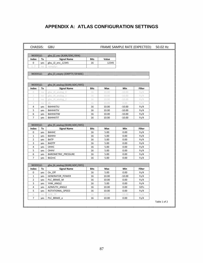
87
APPENDIX A: ATLAS CONFIGURATION SETTINGS
CHASSIS: GBU FRAME SAMPLE RATE (EXPECTED): 50.02 Hz
MODULE: gbu_J2_enc (KAM/ENC/004)
Index Tx Signal Name Bits Value
0 yes gbu_J2_enc_12345 16 12345
1..7 no <empty>
MODULE: gbu_J3_empty (EMPTY/SPARE)
MODULE: gbu_J4_analog (KAM/ADC/005)
Index Tx Signal Name Bits Max Min Filter
0 no gbu_J4_analog_0 16 10.00 -10.00 Fs/4
1 no gbu_J4_analog_1 16 10.00 -10.00 Fs/4
2 no gbu_J4_analog_2 16 10.00 -10.00 Fs/4
3 no db 16 10.00 0.00 Fs/4
4 yes BAHHATIU 16 10.00 -10.00 Fs/4
5 yes BAHHATIV 16 10.00 -10.00 Fs/4
6 yes BAHHATIW 16 10.00 -10.00 Fs/4
7 yes BAHHATIT 16 10.00 -10.00 Fs/4
MODULE: gbu_J5_analog (KAM/ADC/005)
Index Tx Signal Name Bits Max Min Filter
0 yes BAHHC 16 5.00 0.00 Fs/4
1 yes BAHHV 16 5.00 0.00 Fs/4
2 yes BATP 16 5.00 0.00 Fs/4
3 yes BADTP 16 5.00 0.00 Fs/4
4 yes OHHC 16 5.00 0.00 Fs/4
5 yes OHHV 16 5.00 0.00 Fs/4
6 yes BAROMETRIC_PRESSURE 16 5.00 0.00 Fs/4
7 yes BA2mC 16 5.00 0.00 Fs/4
MODULE: gbu_J6_analog (KAM/ADC/005)
Index Tx Signal Name Bits Max Min Filter
0 yes On_Off 16 5.00 0.00 Fs/4
1 yes GENERATOR_POWER 16 10.00 -10.00 Fs/4
2 yes PLC_BRAKE_M 16 10.00 0.00 Fs/4
3 yes YAW_ANGLE 16 5.00 0.00 Fs/4
4 yes AZIMUTH_ANGLE 16 10.00 0.00 32Fs
5 yes ROTATIONAL_SPEED 16 10.00 0.00 Fs/4
6 no SERI_TP 16 10.00 -10.00 Fs/4
7 yes PLC_BRAKE_e 16 10.00 0.00 Fs/4
Table 1 of 2

88
CHASSIS: GBU (continued) FRAME SAMPLE RATE (EXPECTED): 50.02 Hz
MODULE: gbu_J7_analog (KAM/ADC/005)
Index Tx Signal Name Bits Max Min Filter
0 yes BTNACC 16 5.00 0.00 Fs/4
1 yes NACELLE_IMU_AX 16 5.00 0.00 Fs/4
2 yes NACELLE_IMU_AY 16 5.00 0.00 Fs/4
3 yes NACELLE_IMU_AZ 16 5.00 0.00 Fs/4
4 yes NACELLE_IMU_RX 16 5.00 -5.00 Fs/4
5 yes NACELLE_IMU_RY 16 5.00 -5.00 Fs/4
6 yes NACELLE_IMU_RZ 16 5.00 -5.00 Fs/4
7 yes LSS_SPEED 16 10.00 0.00 Fs/4
MODULE: gbu_J8_strain (KAM/ADC/009)
Index Tx Signal Name Bits Max Min Filter ExVolt ExOffset
0 yes TOWER_BENDING_FA 16 0.010 -0.010 Fs/4 5.100 -0.511
1 no gbu_J8_strain_1 16 0.010 -0.010 Fs/4 5.100 0.000
2 yes TOWER_BENDING_SS 16 0.010 -0.010 Fs/4 5.100 0.081
3 no gbu_J8_strain_3 16 0.010 -0.010 Fs/4 5.100 0.000
4 no gbu_J8_strain_4 16 0.010 -0.010 Fs/4 5.100 0.000
5 no gbu_J8_strain_5 16 0.010 -0.010 Fs/4 5.100 0.000
6 no gbu_J8_strain_6 16 0.010 -0.010 Fs/4 5.100 0.000
7 no gbu_J8_strain_7 16 0.010 -0.010 Fs/4 5.100 0.000
MODULE: gbu_J9_analog (KAM/ADC/005)
Index Tx Signal Name Bits Max Min Filter
0 yes BAHHEC 16 5.00 0.00 Fs/4
1 yes BAHHW_Sonic 16 5.00 0.00 Fs/4
2 yes BARTC 16 5.00 0.00 Fs/4
3 yes BARBC 16 5.00 0.00 Fs/4
4 no gbu_J9_analog_0_4 16 5.00 0.00 Fs/4
5 no gbu_J9_analog_0_5 16 5.00 0.00 Fs/4
6 no gbu_J9_analog_0_6 16 5.00 0.00 Fs/4
7 no gbu_J9_analog_0_7 16 10.00 0.00 Fs/4
MODULE: gbu_J10_uar2 (KAM/UAR/002)
Index Tx Signal Name
4 yes TIME_GBU_GPS_Month_Day
6 yes TIME_GBU_GPS_Year
8 yes TIME_GBU_GPS_Hour_Minute
10 yes TIME_GBU_GPS_Second
12 yes TIME_GBU_GPS_Millisecond
Table 2 of 2
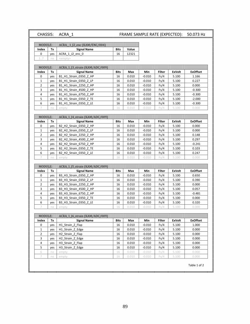
89
CHASSIS: ACRA_1 FRAME SAMPLE RATE (EXPECTED): 50.073 Hz
MODULE: ACRA__1_J2_enc (KAM/ENC/004)
Index Tx Signal Name Bits Value
0 yes ACRA_1_J2_enc_0 16 12321
1..7 no <empty>
MODULE: ACRA_1_J3_strain (KAM/ADC/009)
Index Tx Signal Name Bits Max Min Filter ExVolt ExOffset
0 yes B1_H1_Strain_0350_Z_HP 16 0.010 -0.010 Fs/4 5.100 1.166
1 yes B1_H1_Strain_0350_Z_LP 16 0.010 -0.010 Fs/4 5.100 0.227
2 yes B1_H1_Strain_2250_Z_HP 16 0.010 -0.010 Fs/4 5.100 0.000
3 yes B1_H1_Strain_4500_Z_HP 16 0.010 -0.010 Fs/4 5.100 -0.300
4 yes B1_H1_Strain_6750_Z_HP 16 0.010 -0.010 Fs/4 5.100 -0.300
5 yes B1_H1_Strain_0350_Z_TE 16 0.010 -0.010 Fs/4 5.100 -2.000
6 yes B1_H1_Strain_0350_Z_LE 16 0.010 -0.010 Fs/4 5.100 -0.300
7 no empty 16 0.010 -0.010 Fs/4 5.100 0.000
MODULE: ACRA_1_J4_strain (KAM/ADC/009)
Index Tx Signal Name Bits Max Min Filter ExVolt ExOffset
0 yes B2_H2_Strain_0350_Z_HP 16 0.010 -0.010 Fs/4 5.100 0.000
1 yes B2_H2_Strain_0350_Z_LP 16 0.010 -0.010 Fs/4 5.100 0.000
2 yes B2_H2_Strain_2250_Z_HP 16 0.010 -0.010 Fs/4 5.100 0.148
3 yes B2_H2_Strain_4500_Z_HP 16 0.010 -0.010 Fs/4 5.100 0.297
4 yes B2_H2_Strain_6750_Z_HP 16 0.010 -0.010 Fs/4 5.100 -0.241
5 yes B2_H2_Strain_0350_Z_TE 16 0.010 -0.010 Fs/4 5.100 0.103
6 yes B2_H2_Strain_0350_Z_LE 16 0.010 -0.010 Fs/4 5.100 0.247
7 no empty 16 0.010 -0.010 Fs/4 5.100 0.000
MODULE: ACRA_1_J5_strain (KAM/ADC/009)
Index Tx Signal Name Bits Max Min Filter ExVolt ExOffset
0 yes B3_H3_Strain_0350_Z_HP 16 0.010 -0.010 Fs/4 5.100 0.650
1 yes B3_H3_Strain_0350_Z_LP 16 0.010 -0.010 Fs/4 5.100 0.390
2 yes B3_H3_Strain_2250_Z_HP 16 0.010 -0.010 Fs/4 5.100 0.000
3 yes B3_H3_Strain_4500_Z_HP 16 0.010 -0.010 Fs/4 5.100 0.057
4 yes B3_H3_Strain_6750_Z_HP 16 0.010 -0.010 Fs/4 5.100 -0.481
5 yes B3_H3_Strain_0350_Z_TE 16 0.010 -0.010 Fs/4 5.100 0.000
6 yes B3_H3_Strain_0350_Z_LE 16 0.010 -0.010 Fs/4 5.100 0.320
7 no empty 16 0.010 -0.010 Fs/4 5.100 0.000
MODULE: ACRA_1_J6_strain (KAM/ADC/009)
Index Tx Signal Name Bits Max Min Filter ExVolt ExOffset
0 yes H1_Strain_Z_Flap 16 0.010 -0.010 Fs/4 5.100 1.000
1 yes H1_Strain_Z_Edge 16 0.010 -0.010 Fs/4 5.100 0.000
2 yes H2_Strain_Z_Flap 16 0.010 -0.010 Fs/4 5.100 0.000
3 yes H2_Strain_Z_Edge 16 0.010 -0.010 Fs/4 5.100 0.000
4 yes H3_Strain_Z_Flap 16 0.010 -0.010 Fs/4 5.100 0.000
5 yes H3_Strain_Z_Edge 16 0.010 -0.010 Fs/4 5.100 0.000
6 no empty 16 0.010 -0.010 Fs/4 5.100 0.000
7 no empty 16 0.010 -0.010 Fs/4 5.100 0.000
Table 1 of 2

90
CHASSIS: ACRA_1 (continued) FRAME SAMPLE RATE (EXPECTED): 50.073 Hz
MODULE: ACRA_1_J7_analog (KAM/ADC/005)
Index Tx Signal Name Bits Max Min Filter
0 yes B1_Motor1_Position 16 10.00 0.00 Fs/4
1 yes B1_Motor1_Current 16 10.00 0.00 Fs/4
2 yes B2_Motor1_Position 16 10.00 0.00 Fs/4
3 yes B2_Motor1_Current 16 10.00 0.00 Fs/4
4 yes B3_Motor1_Position 16 10.00 0.00 Fs/4
5 yes B3_Motor1_Current 16 10.00 0.00 Fs/4
6 no empty1 16 10.00 0.00 Fs/4
7 no empty2 16 10.00 0.00 Fs/4
MODULE: ACRA_1_J8_analog (KAM/ADC/005)
Index Tx Signal Name Bits Max Min Filter
0 yes B1_Motor2_Position 16 10.00 0.00 Fs/4
1 yes B1_Motor2_Current 16 10.00 0.00 Fs/4
2 yes B2_Motor2_Position 16 10.00 0.00 Fs/4
3 yes B2_Motor2_Current 16 10.00 0.00 Fs/4
4 yes B3_Motor2_Position 16 10.00 0.00 Fs/4
5 yes B3_Motor2_Current 16 10.00 0.00 Fs/4
6 no empty3 16 10.00 0.00 Fs/4
7 no empty4 16 10.00 0.00 Fs/4
MODULE: ACRA_1_J9_analog (KAM/ADC/012)
Index Tx Signal Name Bits Max Min Filter
0 yes B1_Motor3_Position 16 1.00 0.00 Fs/4
1 yes B1_Motor3_Current 16 1.00 0.00 Fs/4
2 yes B2_Motor3_Position 16 1.00 0.00 Fs/4
3 yes B2_Motor3__Current 16 1.00 0.00 Fs/4
4 yes B3_Motor3_Position 16 1.00 0.00 Fs/4
5 yes B3_Motor3_Current 16 1.00 0.00 Fs/4
6 no empty5 16 1.00 0.00 Fs/4
7 no empty6 16 1.00 0.00 Fs/4
8 yes Athena_AnalogOut1 16 1.00 0.00 Fs/4
9 yes Athena_AnalogOut2 16 1.00 0.00 Fs/4
10 yes Athena_AnalogOut3 16 1.00 0.00 Fs/4
11 yes Cntrlbx_Extra1 16 1.00 0.00 Fs/4
12 yes Cntrlbx_Extra2 16 1.00 0.00 Fs/4
13 .. 19 no empty 16 1.00 0.00 Fs/4
20 yes DAQ_IMU_X 16 1.00 0.00 Fs/4
21 yes DAQ_IMU_Y 16 1.00 0.00 Fs/4
22 yes DAQ_IMU_Z 16 1.00 0.00 Fs/4
23 yes Impact_Hammer 16 1.00 0.00 Fs/4
MODULE: ACRA_1_J10_uar2 (KAM/UAR/002)
Index Tx Signal Name
4 yes Time_GPS_Month_Day
6 yes Time_GPS_Year
8 yes Time_GPS_Hour_Minute
10 yes Time_GPS_Second
12 yes Time_GPS_Millisecond
Table 2 of 2

91
CHASSIS: cRIO_1 FRAME SAMPLE RATE (EXPECTED): 49.98 Hz
MODULE: cRIO_1_J2_ctl (KAM/ENC/004)
Index Tx Signal Name Chassis ID
cRIO_1_J2_ctl_Id_12345 12345
MODULE: cRIO_1_J3_gps (RIO/SEA/GPS)
Index Tx Signal Name
0 yes cRIO_1_J3_gps__Month-Day
1 yes cRIO_1_J3_gps__Year
2 yes cRIO_1_J3_gps__Hour-Minutes
3 yes cRIO_1_J3_gps__Seconds
4 yes cRIO_1_J3_gps__Milliseconds
MODULE: cRIO_1_J4_analog (RIO/ADC/9239)
Index Tx Signal Name Bits Max Min Filter Cutoff Decimation
0 yes B1_H1_Accel_2000_X_HP 24 10.00 -10.00 Butterworth Fs/4 Straight
1 yes B1_H1_Accel_2000_Y_HP 24 10.00 -10.00 Butterworth Fs/4 Straight
2 yes B1_H1_Accel_2000_Z_HP 24 10.00 -10.00 Butterworth Fs/4 Straight
3 yes B1_H1_Accel_2000_X_TE 24 10.00 -10.00 Butterworth Fs/4 Straight
MODULE: cRIO_1_J5_analog (RIO/ADC/9239)
Index Tx Signal Name Bits Max Min Filter Cutoff Decimation
0 yes B1_H1_Accel_8000_X_HP 24 10.00 -10.00 Butterworth Fs/4 Straight
1 yes B1_H1_Accel_8000_Y_HP 24 10.00 -10.00 Butterworth Fs/4 Straight
2 yes B1_H1_Accel_8000_Z_HP 24 10.00 -10.00 Butterworth Fs/4 Straight
3 yes B1_H1_Accel_8000_X_TE 24 10.00 -10.00 Butterworth Fs/4 Straight
MODULE: cRIO_1_J6_analog (RIO/ADC/9239)
Index Tx Signal Name Bits Max Min Filter Cutoff Decimation
0 yes B2_H2_Accel_2000_X_HP 24 10.00 -10.00 Butterworth Fs/4 Straight
1 yes B2_H2_Accel_2000_Y_HP 24 10.00 -10.00 Butterworth Fs/4 Straight
2 yes B2_H2_Accel_2000_Z_HP 24 10.00 -10.00 Butterworth Fs/4 Straight
3 yes B2_H2_Accel_2000_X_TE 24 10.00 -10.00 Butterworth Fs/4 Straight
MODULE: cRIO_1_J7_analog (RIO/ADC/9239)
Index Tx Signal Name Bits Max Min Filter Cutoff Decimation
0 yes B2_H2_Accel_8000_X_HP 24 10.00 -10.00 Butterworth Fs/4 Straight
1 yes B2_H2_Accel_8000_Y_HP 24 10.00 -10.00 Butterworth Fs/4 Straight
2 yes B2_H2_Accel_8000_Z_HP 24 10.00 -10.00 Butterworth Fs/4 Straight
3 yes B2_H2_Accel_8000_X_TE 24 10.00 -10.00 Butterworth Fs/4 Straight
Table 1 of 2

92
CHASSIS: cRIO_1 (continued) FRAME SAMPLE RATE (EXPECTED): 49.98 Hz
MODULE: cRIO_1_J8_analog (RIO/ADC/9239)
Index Tx Signal Name Bits Max Min Filter Cutoff Decimation
0 yes B3_H3_Accel_2000_X_HP 24 10.00 -10.00 Butterworth Fs/4 Straight
1 yes B3_H3_Accel_2000_Y_HP 24 10.00 -10.00 Butterworth Fs/4 Straight
2 yes B3_H3_Accel_2000_Z_HP 24 10.00 -10.00 Butterworth Fs/4 Straight
3 yes B3_H3_Accel_2000_X_TE 24 10.00 -10.00 Butterworth Fs/4 Straight
MODULE: cRIO_1_J9_analog (RIO/ADC/9239)
Index Tx Signal Name Bits Max Min Filter Cutoff Decimation
0 yes B3_H3_Accel_8000_X_HP 24 10.00 -10.00 Butterworth Fs/4 Straight
1 yes B3_H3_Accel_8000_Y_HP 24 10.00 -10.00 Butterworth Fs/4 Straight
2 yes B3_H3_Accel_8000_Z_HP 24 10.00 -10.00 Butterworth Fs/4 Straight
3 yes B3_H3_Accel_8000_X_TE 24 10.00 -10.00 Butterworth Fs/4 Straight
MODULE: cRIO_1_J10_analog (RIO/ADC/9205)
Index Tx Signal Name Bits Max Min Filter Cutoff Decimation
0 yes B1_H1_Strain_0350_Z_HP 16 0.20 -0.20 Butterworth Fs/4 Straight
1 yes B1_H1_Strain_0350_Z_LP 16 0.20 -0.20 Butterworth Fs/4 Straight
2 yes B1_H1_Strain_2250_Z_HP 16 0.20 -0.20 Butterworth Fs/4 Straight
3 yes B1_H1_Strain_4500_Z_HP 16 0.20 -0.20 Butterworth Fs/4 Straight
4 yes B1_H1_Strain_6750_Z_HP 16 0.20 -0.20 Butterworth Fs/4 Straight
5 yes B1_H1_Strain_0350_Z_TE 16 0.20 -0.20 Butterworth Fs/4 Straight
6 yes B1_H1_Strain_0350_Z_LE 16 0.20 -0.20 Butterworth Fs/4 Straight
7 no empty1 16 5.00 -5.00 Butterworth Fs/4 Straight
8 no empty2 16 10.00 -10.00 Butterworth Fs/4 Straight
9 no empty3 16 10.00 -10.00 Butterworth Fs/4 Straight
10 no empty4 16 10.00 -10.00 Butterworth Fs/4 Straight
11 no empty5 16 10.00 -10.00 Butterworth Fs/4 Straight
12 yes DAQ_IMU_X_cRIO 16 10.00 -10.00 Butterworth Fs/4 Straight
13 yes DAQ_IMU_Y_cRIO 16 10.00 -10.00 Butterworth Fs/4 Straight
14 yes DAQ_IMU_Z_cRIO 16 10.00 -10.00 Butterworth Fs/4 Straight
15 yes Impact_Hammer_cRIO 16 10.00 -10.00 Butterworth Fs/4 Straight
Table 2 of 2

93

94
DISTRIBUTION
1 Shreyas Ananthan c/o Ivette Gonzalez
Office of Wind and Water Power Technologies
EE-2B Forrestal Building, U.S. DOE
1000 Independence Ave. SW
Washington, DC 20585
1 Dale Berg
12421 Chelwood Trl NE
Albuquerque, NM 87112
1 Michael Derby c/o Ivette Gonzalez
Office of Wind and Water Power Technologies
EE-2B Forrestal Building, U.S. DOE
1000 Independence Ave. SW
Washington, DC 20585
1 Mark Higgins c/o Ivette Gonzalez
Office of Wind and Water Power Technologies
EE-2B Forrestal Building, U.S. DOE
1000 Independence Ave. SW
Washington, DC 20585
1 Jose Zayas c/o Ivette Gonzalez
Office of Wind and Water Power Technologies
EE-2B Forrestal Building, U.S. DOE
1000 Independence Ave. SW
Washington, DC 20585
1 MS0899 Technical Library 9536 (electronic copy)

95