Embed Size (px)
Citation preview

Purdue UniversityPurdue e-Pubs
Open Access Theses Theses and Dissertations
Spring 2015
Smart V-beltKyle J. MosierPurdue University
Follow this and additional works at: https://docs.lib.purdue.edu/open_access_theses
Part of the Bioresource and Agricultural Engineering Commons, and the MechanicalEngineering Commons
This document has been made available through Purdue e-Pubs, a service of the Purdue University Libraries. Please contact [email protected] foradditional information.
Recommended CitationMosier, Kyle J., "Smart V-belt" (2015). Open Access Theses. 584.https://docs.lib.purdue.edu/open_access_theses/584

i
i


ii
ii
SMART V-BELT
A Thesis
Submitted to the Faculty
of
Purdue University
by
Kyle J. Mosier
In Partial Fulfillment of the
Requirements for the Degree
of
Master of Science
May 2015
Purdue University
West Lafayette, Indiana

ii
ACKNOWLEDGEMENTS
I would like to thank Dr. Gary Krutz for his guidance and support. He has given
me this opportunity and pushed me to work very hard. I would also like to thank Dr.
Robert Stwalley for his direction and overall professionalism during the retirement
transition stage for Dr. Krutz. Thanks to Dr. John Lumkes for being on my graduate
committee and providing crucial feedback and guidance. I would also like to thank
Brittany Newell for all of her help with technical information and guided brainstorming. I
would also like to thank Garry Williams and Scott Brand for all of their help in the
machine shop that made my experiments possible. Thanks to Mathew Ess for his help
collecting raw data in the lab. I need to thank Peter Gibbins of Kirkhill Complete Rubber
Solutions for his invaluable knowledge of rubbers and for supplying my rubber at no
cost. I also need to thank Rick Goetz of Carlisle Transportation Products for donating
belts for use in research. Lastly, I would like to thank Grant Knies for his collaboration
on the project due to the similarity in our topics.
iii
TABLE OF CONTENTS
Page
LIST OF TABLES ............................................................................................................. vi LIST OF FIGURES .......................................................................................................... vii ABSTRACT .............................................................................................................xiv CHAPTER 1. INTRODUCTION ................................................................................. 1
1.1 Objectives ...................................................................................................1
1.2 Purpose of Smart V-Belts ..........................................................................1
1.3 V-Belt Types ..............................................................................................3
1.4 V-Belt Failure Modes ...............................................................................10
CHAPTER 2. LITERATURE REVIEW .................................................................... 14 2.1 Capacitive and Resistive Sensing ............................................................14
2.1.1 Resistive Sensors ...............................................................................14
2.1.2 Capacitive Sensors ............................................................................16
2.2 Prior Research at Purdue University ........................................................22
2.2.1 Hydraulic Hose Sensing ....................................................................22
2.2.2 Tire Sensing ......................................................................................26
2.2.3 Hydraulic O-Ring Seals ....................................................................28
2.2.4 Lumbar Disc Replacement ................................................................30
2.3 Current Belt Sensing Technologies in Industry .......................................31
2.3.1 SensSystems ......................................................................................31
2.3.2 Schrader ............................................................................................33
2.3.3 Tele Haase .........................................................................................33
2.3.4 Honeywell .........................................................................................33
2.3.5 Bridgestone .......................................................................................34
2.3.6 Continental Contitech .......................................................................35
2.4 Vulcanization ...........................................................................................36
CHAPTER 3. SMART V-BELT DESIGN CONCEPTS ........................................... 37 3.1 V-Belt Design Concepts ...........................................................................37
iv
Page
3.2 Sheave Design Concepts ..........................................................................38
CHAPTER 4. INSTRUMENTATION AND PROCEDURES .................................. 43 4.1 Instrumentation ........................................................................................43
4.1.1 Belt Making Instruments ...................................................................43
4.1.2 Belt Testing Instruments ...................................................................53
4.2 Procedures ................................................................................................60
4.2.1 Belt Making Procedures ....................................................................60
4.2.2 Belt Testing Procedures ....................................................................64
CHAPTER 5. TEST RESULTS ................................................................................. 73 5.1 Carlisle Belt Material Tests ......................................................................73
5.2 Carlisle Belt layered Material Flat Plate Tests .........................................74
5.3 Carlisle Belt Hanging Weight Tests .........................................................80
5.4 Carbon Black HNBR Mixture Tests ........................................................81
5.5 Three Inch Belt Section Tests ..................................................................83
CHAPTER 6. CONCLUSIONS AND RECOMMENDATIONS .............................. 94 6.1 Conclusions ..............................................................................................94
6.1.1 Carlisle Belt Material Test Conclusions ...........................................94
6.1.2 Carlisle Belt Flat Plate Test Conclusions ..........................................95
6.1.3 Carlisle Belt Hanging Weight Test Conclusions ..............................95
6.1.4 Conductive Rubber Conclusions .......................................................96
6.1.5 Three Inch Belt Section Test Conclusions ........................................96
6.1.6 Smart V-Belt Research Conclusions .................................................98
6.2 Recommendations ....................................................................................99
6.2.1 Additional Testing and Research ......................................................99
6.2.2 Full Data Acquisition System .........................................................100
BIBLIOGRAPHY ........................................................................................................... 101 APPENDICES
Appendix A ANOVA and Tukey Tests for Flat Plate Data ........................................105
Appendix B ANOVA and Tukey Tests for Hanging Weight Tests ............................106
Appendix C ANOVA and Tukey Tests for 3 Inch Belt Section Data .........................107
Appendix D Material Data and Safety Sheets .............................................................116

v
Page
Appendix E Original Belt and Sheave Designs ...........................................................141
Appendix F Data Acquisition PowerPoint ..................................................................145
vi
LIST OF TABLES
Table .............................................................................................................................. Page
Table 1-1: Classic v-belt sizes (Belarus, 2014) .................................................................. 4
Table 1-2: Classic banded v-belt sizes (Belarus, 2014) ...................................................... 5
Table 1-3: Classic cogged v-belt sizes (Belarus, 2014) ...................................................... 6
Table 1-4: Double angled v-belt sizes (Belarus, 2014) ....................................................... 7
Table 1-5: Variable speed v-belt sizes (Belarus, 2014) ...................................................... 8
Table 1-6: Wedge v-belt sizes (Belarus, 2014) ................................................................... 9
Table 5-1 Percent changes in readings after damages for flat plate tests ......................... 79
Table 5-2 Percent changes in readings after damages for sheave sensing configurations of
three inch samples ............................................................................................................. 91
Table 5-3 Percent changes in readings after damages for layer configurations of three
inch samples ...................................................................................................................... 92
Table 5-4 Coefficient of variation for capacitance and resistance measurements ............ 93
vii
LIST OF FIGURES
Figure ............................................................................................................................. Page
Figure 1-1 Classic V-belt shape (Belarus, 2014) ................................................................ 3
Figure 1-2: Classic banded v-belt (Belarus, 2014) ............................................................. 4
Figure 1-3: Classic cogged v-belt (Belarus, 2014) ............................................................. 5
Figure 1-4: Classic Cogged Banded BX,CX (Belarus, 2014) ............................................ 6
Figure 1-5: Double angled v-belt (Belarus, 2014) .............................................................. 6
Figure 1-6: Variable speed v-belt (Belarus, 2014) .............................................................. 7
Figure 1-7: Wedge v-belt (Belarus, 2014) .......................................................................... 8
Figure 1-8: Cogged Wedge 3VX,5VX (Belarus, 2014) ..................................................... 9
Figure 1-9: Classic Cogged Wedge Banded 3VX,5VX V-Belts (Belarus, 2014) .............. 9
Figure 1-10: Serpentine belt (Belarus, 2014) ...................................................................... 9
Figure 1-11 V-Belt top damage ........................................................................................ 11
Figure 1-12 V-Belt bottom damage .................................................................................. 12
Figure 1-13 V-Belt side damage ....................................................................................... 13
Figure 2-1 Wheatstone Bridge (Engineer's Edge, 2014) .................................................. 15
Figure 2-2 Physical changes affecting capacitance (Gallien, 2008) ................................. 17
Figure 2-3 ‘Fairly Complete Capacitor Model’ (Dr. Krutz, Dr. Timu, Dr. Newell, &
Stewart, 2013) ................................................................................................................... 18
viii
Figure ............................................................................................................................. Page
Figure 2-4 ‘Simplified Capacitance Model’ (Dr. Krutz, Dr. Timu, Dr. Newell, & Stewart,
2013) ................................................................................................................................. 19
Figure 2-5 Inverting Amplifier Configuration (Holland M. , 2007) ................................. 20
Figure 2-6 Inverting amplifier circuit with ideal capacitors (Holland M. , 2007) ............ 21
Figure 2-7 Inverting amplifier circuit with simplified capacitor model (Holland M. ,
2007) ................................................................................................................................. 22
Figure 2-8 Drawing of a Preliminary Design for Life Sense Hose (Holland Z. , 2010) ... 23
Figure 2-9 Experimental Capacitance and static pressure relationship (Deckard, 2004) . 24
Figure 2-10 Capacitance of Hose during Pressure Cycle Failure (Deckard, 2004) .......... 25
Figure 2-11 Capacitance Measurements during Inflation of Research Tire (Holland M. ,
2007) ................................................................................................................................. 26
Figure 2-12 Oscilloscope Voltage Measurements Before and After Damage (Holland M. ,
2007) ................................................................................................................................. 27
Figure 2-13 Load Test of Research O-Rings BI10 and BJ10 (Gallien, 2008) .................. 29
Figure 2-14 Capacitance Measurements Before and After Specific Damages (Gallien,
2008) ................................................................................................................................. 30
Figure 2-15 Diagram (left) and Photograph (right) of the slip monitoring system (Brown,
2012) ................................................................................................................................. 32
Figure 2-16 Drawing of possible BeltAIS configuration (Honeywell, 2012). ................. 34
Figure 2-17 Drawing of Bridgestone’s Monitrix System (Bridgestone, 2015) ................ 35
Figure 2-18 (Continental, 2014) ....................................................................................... 36
Figure 3-1 Proposed V-Belt Constructions ....................................................................... 37

ix
Figure ............................................................................................................................. Page
Figure 3-2 Sheave Design Concept One ........................................................................... 39
Figure 3-3 Sheave Design Concept Two .......................................................................... 40
Figure 3-4 Sheave Design Concept Three ........................................................................ 41
Figure 3-5 Sheave Design Concept Four .......................................................................... 42
Figure 4-1 Dimensions of a layered 5L V-belt ................................................................. 43
Figure 4-2 The three long molds for creating belt layers .................................................. 44
Figure 4-3 Engineering drawing of long mold 1 .............................................................. 45
Figure 4-4 Engineering drawing of long mold 2 .............................................................. 45
Figure 4-5 Engineering drawing of long mold 3 .............................................................. 46
Figure 4-6 .......................................................................................................................... 47
Figure 4-7 Engineering drawing of round mold bottom ................................................... 47
Figure 4-8 Engineering drawing of round mold top ......................................................... 48
Figure 4-9 Three inch belt section mold ........................................................................... 48
Figure 4-10 Engineering drawing of 3-inch belt section mold ......................................... 49
Figure 4-11 OTC 50 ton press in use pressing a long mold.............................................. 50
Figure 4-12 VT-1100 heat gun in use on press (left) and full view of heat gun (right) ... 50
Figure 4-13 shaker in use for mixing conductive rubber .................................................. 51
Figure 4-14 Incubator in use for drying rubber ................................................................ 52
Figure 4-15 American Scientific Products DN-42 Oven .................................................. 53
Figure 4-16 Capacitance Circuit Model Selection (Technologies, 2003) ......................... 54
Figure 4-17 Four Terminal Pair Measurement Configuration (Technologies, 2003) ....... 56
Figure 4-18 Techniques to Reduce Error (Technologies, 2003) ....................................... 57
x
Figure ............................................................................................................................. Page
Figure 4-19 Hewlett Packard 4263B Agilent LCR meter with four terminal pair
configuration ..................................................................................................................... 58
Figure 4-20 Smart V-Belt Test Stand ............................................................................... 59
Figure 4-21 Large Plastic Sheave ..................................................................................... 59
Figure 4-22 Small Plastic Sheave ..................................................................................... 60
Figure 4-23 Examples of the most successful belt Prototypes(top) and the 3 inch belt
sections(bottom) ................................................................................................................ 61
Figure 4-24 Pressed black and red HNBR for three inch sections ................................... 64
Figure 4-25 Carlisle Belt Broken Down Materials Being Tested ..................................... 65
Figure 4-26 Flat Plate Tests of current belt sections......................................................... 66
Figure 4-27 Hanging Weight V-Belt Testing Apparatus .................................................. 67
Figure 4-28 Conductive rubber sample with testing positions marked ............................ 68
Figure 4-29 Three inch v-belt section with copper tape sensor areas and sensing schemes
marked............................................................................................................................... 69
Figure 4-30 Three inch v-belt sections showing the six different layered options tested . 70
Figure 4-31 Pictures of testing(left), short correction(top), and open correction(bottom)
being conducted ................................................................................................................ 71
Figure 4-32 The layer separation(left), hole(middle), and abrasion(right) being inflicted72
Figure 5-1 Pictorial representation of the Carlisle v-belt material testing results ............ 74
Figure 5-2 Resistance readings of flat plate test 1 vs damage with 95% CI ..................... 75
Figure 5-3 Resistance readings of flat plate test 2 vs damage with 95% CI ..................... 75
Figure 5-4 Resistance readings of flat plate test 3 vs damage with 95% CI ..................... 76
xi
Figure ............................................................................................................................. Page
Figure 5-5 Resistance readings of flat plate test 4 vs damage with 95% CI ..................... 76
Figure 5-6 Capacitance readings of flat plate test 1 vs damage with 95% CI .................. 77
Figure 5-7 Capacitance readings of flat plate test 2 vs damage with 95% CI .................. 78
Figure 5-8 Capacitance readings of flat plate test 3 vs damage with 95% CI .................. 78
Figure 5-9 Capacitance readings of flat plate test 4 vs damage with 95% CI .................. 79
Figure 5-10 Resistance readings of Carlisle belt vs weight hung from the belt ............... 80
Figure 5-11 Resistance readings of Carlisle belt vs weight hung from the belt ............... 81
Figure 5-12 Resistance readings across thickness of conductive rubber samples ............ 82
Figure 5-13 Resistance readings through the length of the conductive rubber samples ... 83
Figure 5-14 Resistance test results for three inch belt section 1 tests with 95% CI ......... 84
Figure 5-15 Resistance test results for three inch belt section 2 tests with 95% CI ......... 84
Figure 5-16 Resistance test results for three inch belt section 3 tests with 95% CI ......... 85
Figure 5-17 Resistance test results for three inch belt section 4 tests with 95% CI ......... 85
Figure 5-18 Resistance test results for three inch belt section 5 tests with 95% CI ......... 86
Figure 5-19 Resistance test results for three inch belt section 6 tests with 95% CI ......... 86
Figure 5-20 Capacitance test results for three inch belt section 1 tests with 95% CI ....... 87
Figure 5-21 Capacitance test results for three inch belt section 2 tests with 95% CI ....... 88
Figure 5-22 Capacitance test results for three inch belt section 3 tests with 95% CI ....... 88
Figure 5-23 Capacitance test results for three inch belt section 4 tests with 95% CI ....... 89
Figure 5-24 Capacitance test results for three inch belt section 5 tests with 95% CI ....... 89
Figure 5-25 Capacitance test results for three inch belt section 6 tests with 95% CI ....... 90
Figure D-1 Original Kirkhill Black HNBR Data Sheet Page 1 ...................................... 116

xii
Figure ............................................................................................................................. Page
Figure D-2 Original Kirkhill Black HNBR Data Sheet Page 2 ...................................... 117
Figure D-3 Original Kirkhill Black HNBR Data Sheet Page 3 ...................................... 118
Figure D-4 Original Kirkhill Red HNBR Data Sheet Page 1 ......................................... 119
Figure D-5 Original Kirkhill Red HNBR Data Sheet Page 2 ......................................... 120
Figure D-6 Original Kirkhill Red HNBR Data Sheet Page 3 ......................................... 121
Figure D-7 New Kirkhill Black HNBR Data Sheet Page 1 ............................................ 122
Figure D-8 New Kirkhill Black HNBR Data Sheet Page 2 ............................................ 123
Figure D-9 New Kirkhill Black HNBR Data Sheet Page 3 ............................................ 124
Figure D-10 New Kirkhill Red HNBR Data Sheet Page 1 ............................................. 125
Figure D-11 New Kirkhill Red HNBR Data Sheet Page 2 ............................................. 126
Figure D-12 New Kirkhill Red HNBR Data Sheet Page 3 ............................................. 127
Figure D-13 MEK Material Safety Sheet Page 1 ............................................................ 128
Figure D-14 MEK Material Safety Sheet Page 2 ............................................................ 129
Figure D-15 MEK Material Safety Sheet Page 3 ............................................................ 130
Figure D-16 MEK Material Safety Sheet Page 4 ............................................................ 131
Figure D-17 MEK Material Safety Sheet Page 5 ............................................................ 132
Figure D-18 MEK Material Safety Sheet Page 6 ............................................................ 133
Figure D-19 MEK Material Safety Sheet Page 7 ............................................................ 134
Figure D-20 MEK Material Safety Sheet Page 8 ............................................................ 135
Figure D-21 Whacker Chemie Elastosil RT 622 Data Sheet .......................................... 136
Figure D-22 Whacker Chemie Elastosil RT 625 Data Sheet .......................................... 137
Figure D-23 Zoflex Rubber Material Safety Sheet Page 1 ............................................. 138

xiii
Figure ............................................................................................................................. Page
Figure D-24 Zoflex Rubber Material Safety Sheet Page 2 ............................................. 139
Figure D-25 Zoflex Rubber Data Sheet .......................................................................... 140
Figure E-26 Original Belt Design Side to Side with Embedded Copper ........................ 141
Figure E-27 Original Belt Design Side to Side with Embedded Copper and Wireless .. 141
Figure E-28 Original Belt Design Side to Side with Conductive Fabric Layer .............. 142
Figure E-29 Original Belt Design Top to Bottom with Embedded Copper ................... 142
Figure E-30 Original Belt Design Top to Bottom with Embedded Copper and Wireless
......................................................................................................................................... 143
Figure E-31 Original Belt and Sheave Design Mid to Top with Conductive Rubber and
Idler ................................................................................................................................. 143
Figure E-32 Original Sheave Design with Gap for Sensing on one Pulley .................... 144
Figure E-33 Original Sheave Design Fist Idler Configuration Idea ............................... 144
Figure E-34 Original Sheave Design with Insulation Built into Sheave. ....................... 145
Figure F-35 Data Acquisition PowerPoint Slides ........................................................... 147
...............................................................................................................................................
xiv
xiv
ABSTRACT
Mosier, Kyle J. M.S., Purdue University, May 2015. Smart V-belt. Major Professors: Dr.
Gary W. Krutz and Dr. Robert Stwalley.
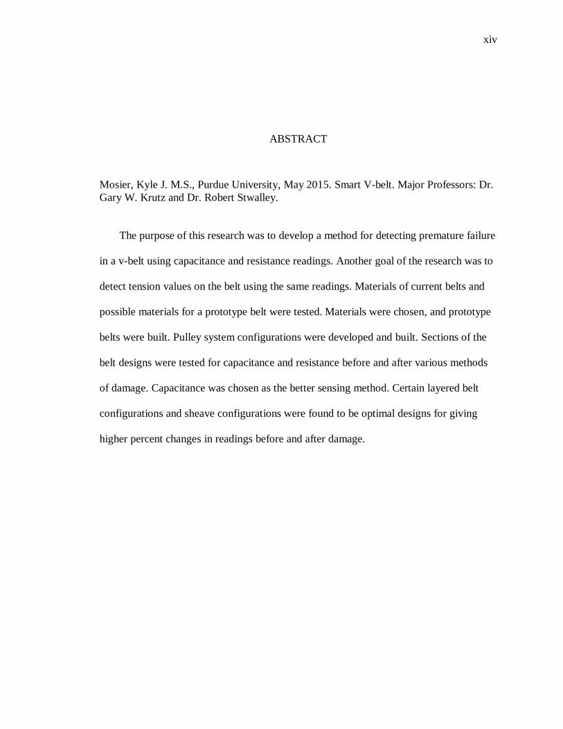
The purpose of this research was to develop a method for detecting premature failure
in a v-belt using capacitance and resistance readings. Another goal of the research was to
detect tension values on the belt using the same readings. Materials of current belts and
possible materials for a prototype belt were tested. Materials were chosen, and prototype
belts were built. Pulley system configurations were developed and built. Sections of the
belt designs were tested for capacitance and resistance before and after various methods
of damage. Capacitance was chosen as the better sensing method. Certain layered belt
configurations and sheave configurations were found to be optimal designs for giving
higher percent changes in readings before and after damage.
1
CHAPTER 1. INTRODUCTION
1.1 Objectives
The main goal was to develop a technology to detect failure of a v-belt
prematurely. Here was the list of more specific objectives regarding this research.
1. The technology needed to be a relatively cheap and simple solution compared to
current solutions.
2. The solution needed to be able to detect failure in the tension cord area.
3. The sensor should be able to detect cracking in the belt.
4. The technology should be able to detect changes in the tension on the belt.
1.2 Purpose of Smart V-Belts
The purpose of smart V-belts was to be able to prematurely detect a failure.
Catastrophic belt failure can halt productivity in many industries. This kind of failure
creates much more downtime than simply stopping to change a worn or damaged belt. A
couple of examples applications for a smart v-belt would be in a combine and in a food
manufacturing plant. In the case of a belt failure in a combine, the farmer has the
potential to be stranded out in the middle of a field with a broken belt. This costs him
extra time to get out of the field and extra money to get the replacement installed on-site
or have the equipment towed out of the field for repair. In a food manufacturing plant, a
catastrophic failure of a belt could expel shards of rubber and contaminate whole batches

2
of food product. This will not only cause downtime for clean-up and repair, but massive
amounts of contaminated food will have to be discarded. The problem of catastrophic belt
failures can be solved by using Smart Belts that can be monitored and removed when
damage is detected prior to complete failure.
Another purpose of smart v-belts was for manufacturers of belts that have the
issue of manufacturing quality control. This is a major issue. If the product cannot be
guaranteed by some sort of quality check before leaving the factory, the manufacturer is
responsible for any damages that can be said to have been caused by a defective belt. The
financial and reputational costs of being blamed for a manufacturing defect can be
extremely high. Improved quality control is a benefit of this technology.
There are currently very few ways to monitor belt condition in industry. One was
to inspect the belt each time before it was to be used. This has been a very time intensive
process as the belts usually were protected and would have to be uncovered, checked, and
recovered before each use. This was also a very subjective and unreliable process.
Visual inspection technologies have been developed to remove the human from
the process and greatly decrease time to inspect the belt. This technology does not give
direct information from inside the belt regarding condition. This is also an expensive
technology due to the high speed and high definition cameras used and extensive
algorithms needed to classify and detect damages.
Another inexpensive and popular method has been to measure slip. This was done
in a few ways such as measuring heat produced by slippage and ratio of loaded and
driven sheave rotational speeds. This measure is an indicator of belt condition, but it is
secondary and does not give direct information about the internal condition of the belt.
3
Other more inclusive ways of detecting failure are very expensive and
cumbersome technologies that monitor the belt. These technologies will be discussed in
the literature review.
1.3 V-Belt Types
There are many different types of v-belts. The main categories break them down
by sizes offered and shape. Variations include classic, double angled, wedge, variable
speed, metric, specialty, and micro-rib or serpentine v-belts.
There are eight different section classifications of classic v-belts indicating the
height and top width. Classic v-belts have so many variations in materials used,
manufacturing processes, size, and shape that it would be difficult to cover them all.
Some have a protective fabric wrap some do not. Some have no tension cords, and others
have many different materials for tension cords such as metal, polyester, and aramid,
which is also known as Kevlar. The most commonly used variations will be discussed.
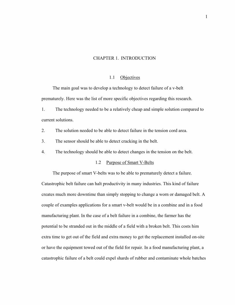
Classic v-belts are the most commonly used type of belt. These are used for their
low noise and vibration compared to a chain. They also allow limited slip which is
beneficial in a situation where timing is not an issue and over-speeding or over-torqueing
could be a problem. Figure 1-1 shows an example of a simple classic v-belt shape. Table
1-1 shows the dimensions of simple classic belt cross-sections and their names. The “L”
sizes are the light duty belts. The A through E are general purpose heavy duty belts.
Figure 1-1 Classic V-belt shape (Belarus, 2014)
4
Table 1-1: Classic v-belt sizes (Belarus, 2014)
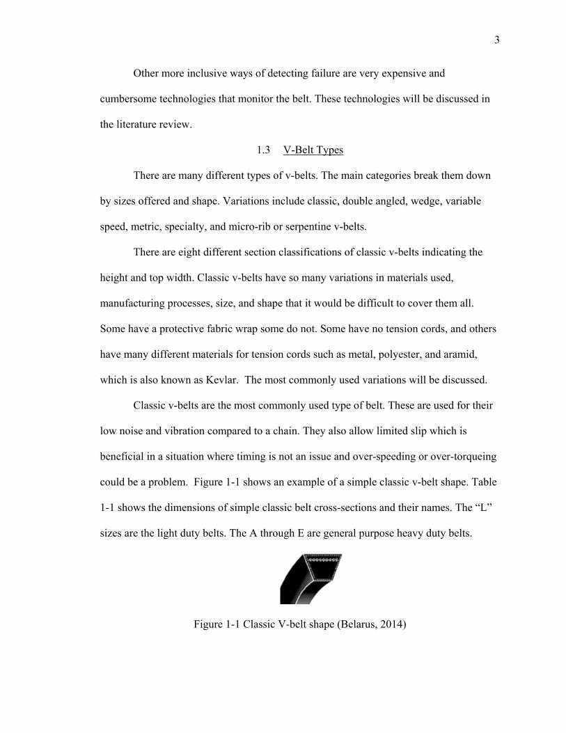
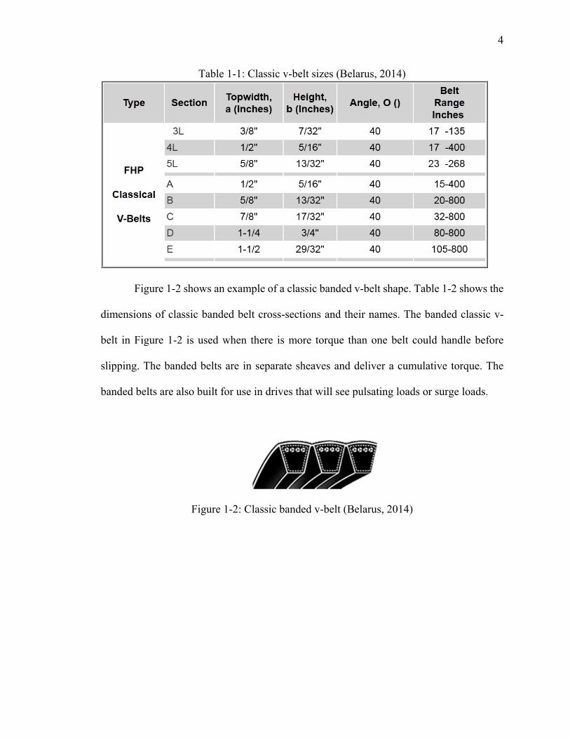
Figure 1-2 shows an example of a classic banded v-belt shape. Table 1-2 shows the
dimensions of classic banded belt cross-sections and their names. The banded classic v-
belt in Figure 1-2 is used when there is more torque than one belt could handle before
slipping. The banded belts are in separate sheaves and deliver a cumulative torque. The
banded belts are also built for use in drives that will see pulsating loads or surge loads.
Figure 1-2: Classic banded v-belt (Belarus, 2014)
5
Table 1-2: Classic banded v-belt sizes (Belarus, 2014)
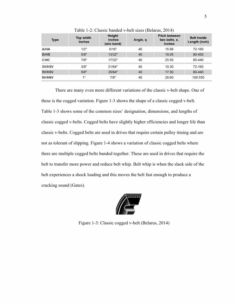
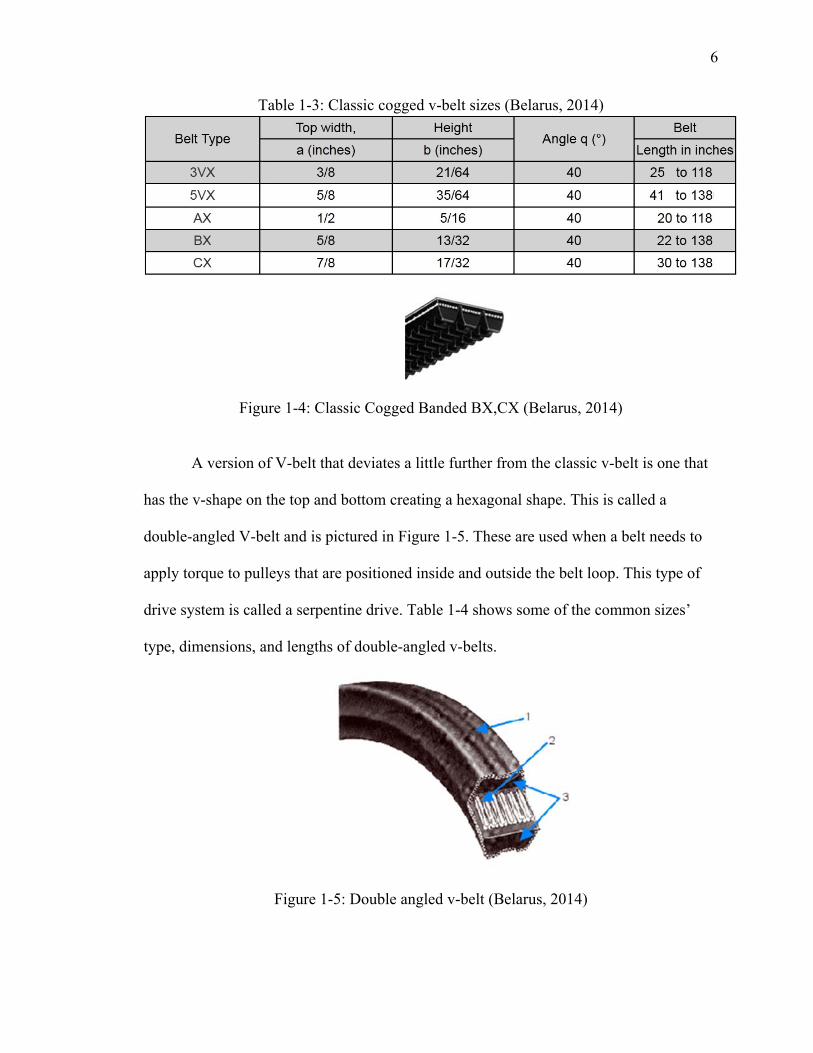
There are many even more different variations of the classic v-belt shape. One of
these is the cogged variation. Figure 1-3 shows the shape of a classic cogged v-belt.
Table 1-3 shows some of the common sizes’ designation, dimensions, and lengths of
classic cogged v-belts. Cogged belts have slightly higher efficiencies and longer life than
classic v-belts. Cogged belts are used in drives that require certain pulley timing and are
not as tolerant of slipping. Figure 1-4 shows a variation of classic cogged belts where
there are multiple cogged belts banded together. These are used in drives that require the
belt to transfer more power and reduce belt whip. Belt whip is when the slack side of the
belt experiences a shock loading and this moves the belt fast enough to produce a
cracking sound (Gates).
Figure 1-3: Classic cogged v-belt (Belarus, 2014)
6
Table 1-3: Classic cogged v-belt sizes (Belarus, 2014)
Figure 1-4: Classic Cogged Banded BX,CX (Belarus, 2014)
A version of V-belt that deviates a little further from the classic v-belt is one that
has the v-shape on the top and bottom creating a hexagonal shape. This is called a
double-angled V-belt and is pictured in Figure 1-5. These are used when a belt needs to
apply torque to pulleys that are positioned inside and outside the belt loop. This type of
drive system is called a serpentine drive. Table 1-4 shows some of the common sizes’
type, dimensions, and lengths of double-angled v-belts.
Figure 1-5: Double angled v-belt (Belarus, 2014)

7
Table 1-4: Double angled v-belt sizes (Belarus, 2014)
Variable speed v-belts are another variation of the classical v-belt. These are
essentially wider versions of cogged classical v-belts. This shape is depicted in Figure 1-
6. These belts are able to handle changes in speed better than classic v-belts or classic
cogged belts. Table 1-5 shows some of the common sizes’ designation, dimensions, and
lengths of variable speed v-belts.
Figure 1-6: Variable speed v-belt (Belarus, 2014)
8
Table 1-5: Variable speed v-belt sizes (Belarus, 2014)
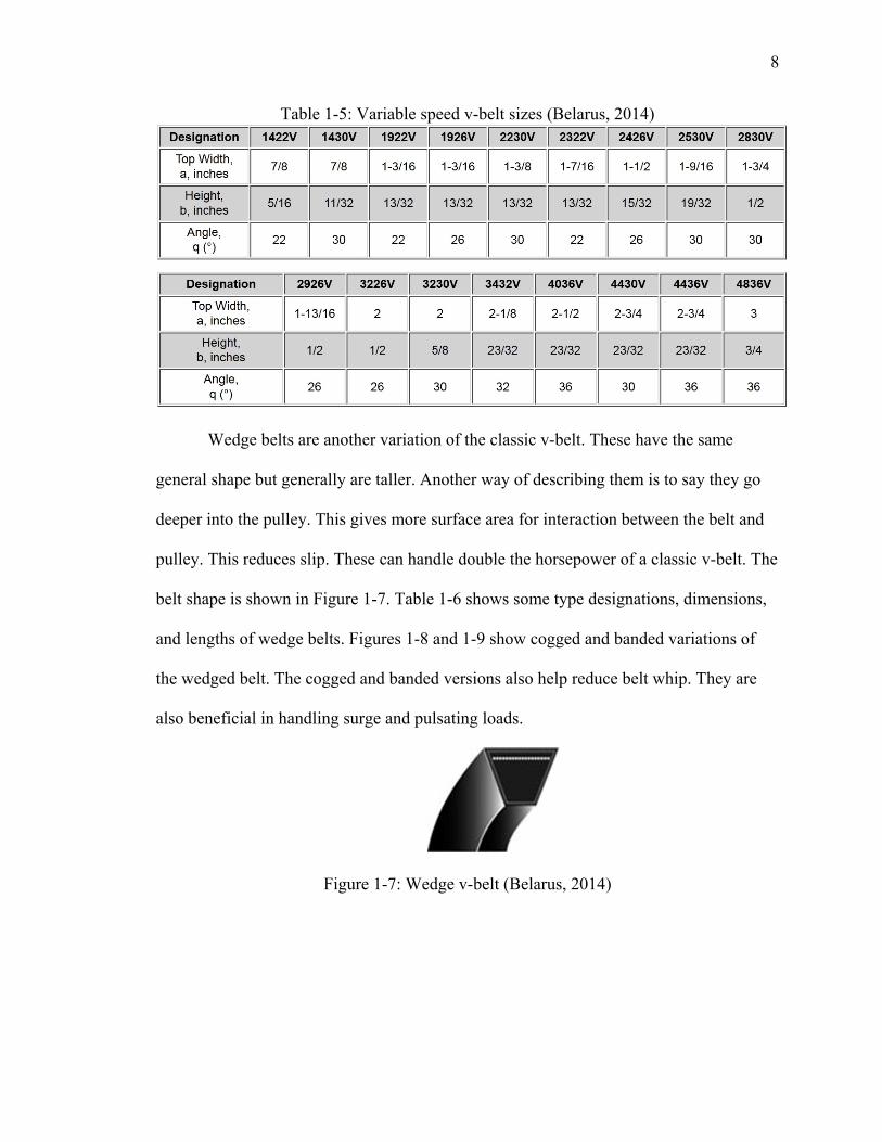
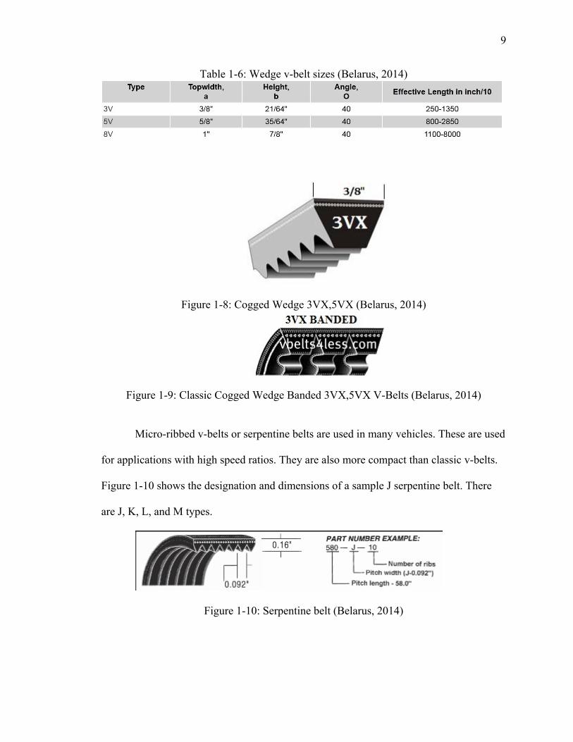
Wedge belts are another variation of the classic v-belt. These have the same
general shape but generally are taller. Another way of describing them is to say they go
deeper into the pulley. This gives more surface area for interaction between the belt and
pulley. This reduces slip. These can handle double the horsepower of a classic v-belt. The
belt shape is shown in Figure 1-7. Table 1-6 shows some type designations, dimensions,
and lengths of wedge belts. Figures 1-8 and 1-9 show cogged and banded variations of
the wedged belt. The cogged and banded versions also help reduce belt whip. They are
also beneficial in handling surge and pulsating loads.
Figure 1-7: Wedge v-belt (Belarus, 2014)
9
Table 1-6: Wedge v-belt sizes (Belarus, 2014)
Figure 1-8: Cogged Wedge 3VX,5VX (Belarus, 2014)
Figure 1-9: Classic Cogged Wedge Banded 3VX,5VX V-Belts (Belarus, 2014)
Micro-ribbed v-belts or serpentine belts are used in many vehicles. These are used
for applications with high speed ratios. They are also more compact than classic v-belts.
Figure 1-10 shows the designation and dimensions of a sample J serpentine belt. There
are J, K, L, and M types.
Figure 1-10: Serpentine belt (Belarus, 2014)
10
There are also metric sizes of v-belts that have not been depicted or identified
with exact dimensions. The belts described here cover the basic and the most commonly
used types of v-belts.
1.4 V-Belt Failure Modes
An understanding of the possible ways a v-belt can fail is crucial to the research
of smart v-belts. For the purpose of this research the damages and failures have been
categorized into the regions of the belt that they occur.
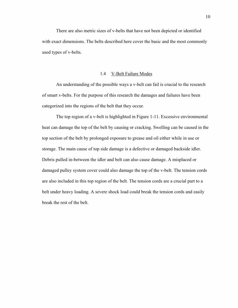
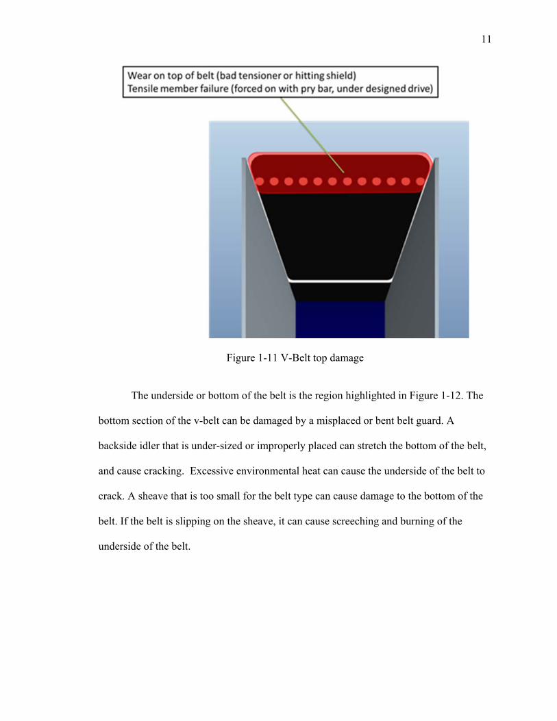
The top region of a v-belt is highlighted in Figure 1-11. Excessive environmental
heat can damage the top of the belt by causing or cracking. Swelling can be caused in the
top section of the belt by prolonged exposure to grease and oil either while in use or
storage. The main cause of top side damage is a defective or damaged backside idler.
Debris pulled in-between the idler and belt can also cause damage. A misplaced or
damaged pulley system cover could also damage the top of the v-belt. The tension cords
are also included in this top region of the belt. The tension cords are a crucial part to a
belt under heavy loading. A severe shock load could break the tension cords and easily
break the rest of the belt.
11
Figure 1-11 V-Belt top damage
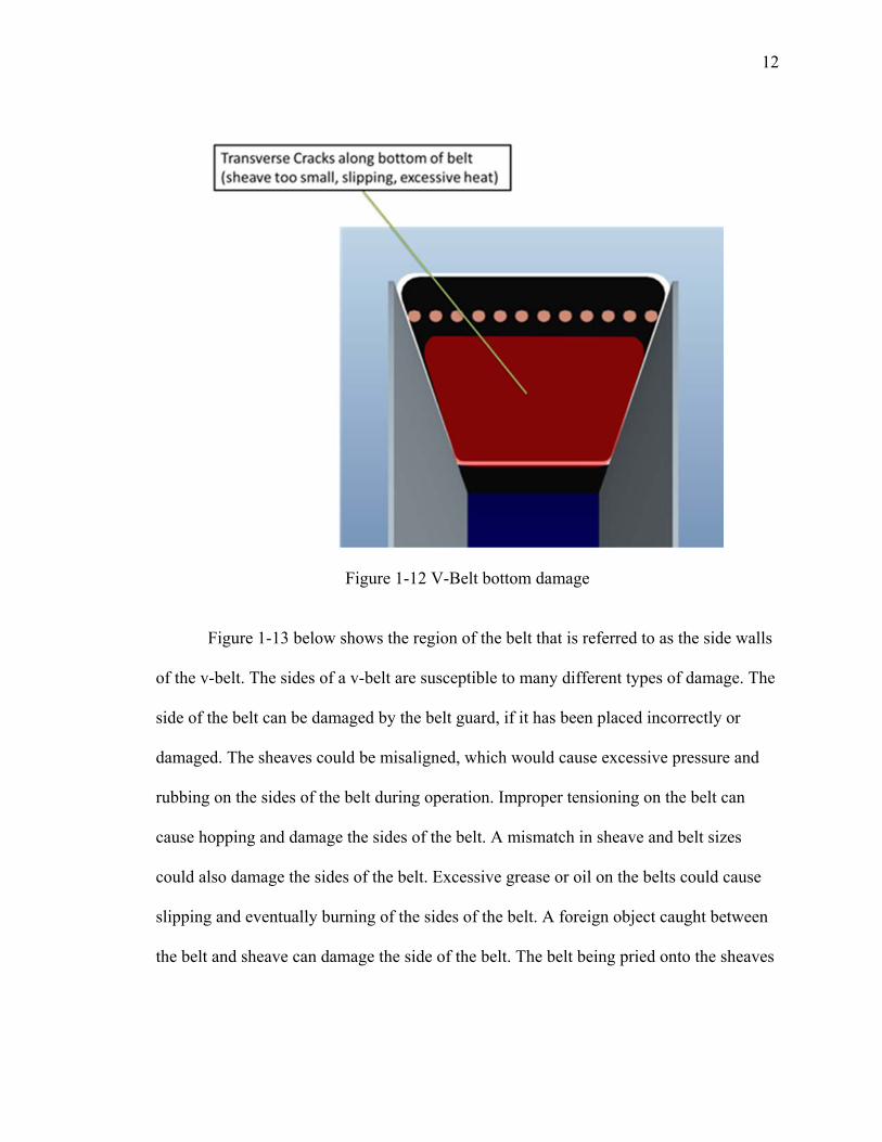
The underside or bottom of the belt is the region highlighted in Figure 1-12. The
bottom section of the v-belt can be damaged by a misplaced or bent belt guard. A
backside idler that is under-sized or improperly placed can stretch the bottom of the belt,
and cause cracking. Excessive environmental heat can cause the underside of the belt to
crack. A sheave that is too small for the belt type can cause damage to the bottom of the
belt. If the belt is slipping on the sheave, it can cause screeching and burning of the
underside of the belt.
12
Figure 1-12 V-Belt bottom damage
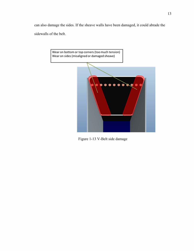
Figure 1-13 below shows the region of the belt that is referred to as the side walls
of the v-belt. The sides of a v-belt are susceptible to many different types of damage. The
side of the belt can be damaged by the belt guard, if it has been placed incorrectly or
damaged. The sheaves could be misaligned, which would cause excessive pressure and
rubbing on the sides of the belt during operation. Improper tensioning on the belt can
cause hopping and damage the sides of the belt. A mismatch in sheave and belt sizes
could also damage the sides of the belt. Excessive grease or oil on the belts could cause
slipping and eventually burning of the sides of the belt. A foreign object caught between
the belt and sheave can damage the side of the belt. The belt being pried onto the sheaves
13
can also damage the sides. If the sheave walls have been damaged, it could abrade the
sidewalls of the belt.
Figure 1-13 V-Belt side damage

14
CHAPTER 2. LITERATURE REVIEW
2.1 Capacitive and Resistive Sensing
A sensor is a tool that provides an electric output corresponding to an observed
physical quantity. Capacitive and resistive sensors are currently used in many different
applications. Resistive sensors are used as force sensors, strain gauges, photoresistors,
and many more sensing applications. Capacitive sensors are used as pressure sensors,
thickness sensors, dynamic motion sensors, and used in a multitude of other sensing
applications. These are two types of sensing that are crucial to smart v-belt research.
2.1.1 Resistive Sensors
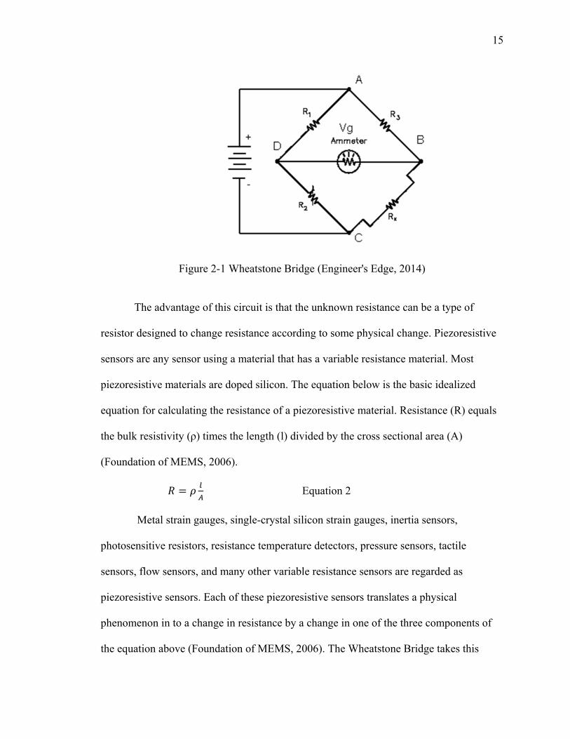
Many resistance type sensors use a Wheatstone Bridge similar to the one pictured
below in Figure 2-1 Wheatstone Bridge . The bridge consists of three resistors of known
resistance, one resistor of unknown resistance, a voltage source and an ammeter. This
ammeter is used to measure the current across D to B. The current information is not as
useful as the voltage. For this reason, the current is usually converted to voltage using
Ohm’s law which is equation shown below where voltage (V) equals the current (I) times
resistance (R). The ammeter has a known resistance associated with it, so the voltage can
be easily calculated Engineer'sEdge, 2009 .
∗ Equation 1
15
Figure 2-1 Wheatstone Bridge (Engineer's Edge, 2014)
The advantage of this circuit is that the unknown resistance can be a type of
resistor designed to change resistance according to some physical change. Piezoresistive
sensors are any sensor using a material that has a variable resistance material. Most
piezoresistive materials are doped silicon. The equation below is the basic idealized
equation for calculating the resistance of a piezoresistive material. Resistance (R) equals
the bulk resistivity (ρ) times the length (l) divided by the cross sectional area (A)
(Foundation of MEMS, 2006).
Equation 2
Metal strain gauges, single-crystal silicon strain gauges, inertia sensors,
photosensitive resistors, resistance temperature detectors, pressure sensors, tactile
sensors, flow sensors, and many other variable resistance sensors are regarded as
piezoresistive sensors. Each of these piezoresistive sensors translates a physical
phenomenon in to a change in resistance by a change in one of the three components of
the equation above (Foundation of MEMS, 2006). The Wheatstone Bridge takes this

16
change in resistance and translates it into a change in voltage. This voltage can be read
directly on an output screen or can be recorded by a data acquisition system.
2.1.2 Capacitive Sensors
Capacitance sensors are similar to piezoresistive sensors, because they generate
an electric signal from the deformation of a membrane. The difference is that a capacitive
sensor uses displacement of the membrane to create the signal, rather than the stress in
the membrane. Many capacitive sensors are modified parallel plate capacitors. Parallel
plate capacitors consist of two electrodes, or plates, and dielectric material between the
plates. Equation 3 shows the basic equation that governs capacitance behavior. C,
measured in Farads, is the capacitance and is affected by four factors. ‘ε’ is the dielectric
constant of the material between the plates, and is unit-less. ‘ ’ is the permittivity of free
space, and is in units of Farads over meters. ‘A’ is the area of overlap of the plates,
measured in meters squared. ‘D’ is the distance between the plates, measured in meters.
(Gallien, 2008)
Equation 3
In these parallel plate capacitors there are three main ways of physically changing
the capacitor and in turn changing capacitance. The changes to capacitance are governed
by Equation 3. If the dielectric constant ( ) of the material between the plates is changed
the capacitance is affected proportionally. A change in the distance between the plates
(D) inversely changes the resulting capacitance. A change in the area of plate overlap (A)
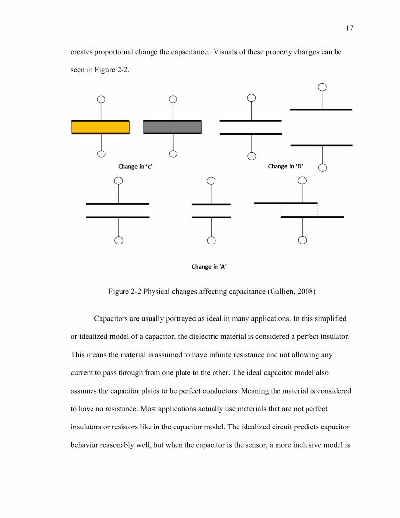
17
creates proportional change the capacitance. Visuals of these property changes can be
seen in Figure 2-2.
Figure 2-2 Physical changes affecting capacitance (Gallien, 2008)
Capacitors are usually portrayed as ideal in many applications. In this simplified
or idealized model of a capacitor, the dielectric material is considered a perfect insulator.
This means the material is assumed to have infinite resistance and not allowing any
current to pass through from one plate to the other. The ideal capacitor model also
assumes the capacitor plates to be perfect conductors. Meaning the material is considered
to have no resistance. Most applications actually use materials that are not perfect
insulators or resistors like in the capacitor model. The idealized circuit predicts capacitor
behavior reasonably well, but when the capacitor is the sensor, a more inclusive model is
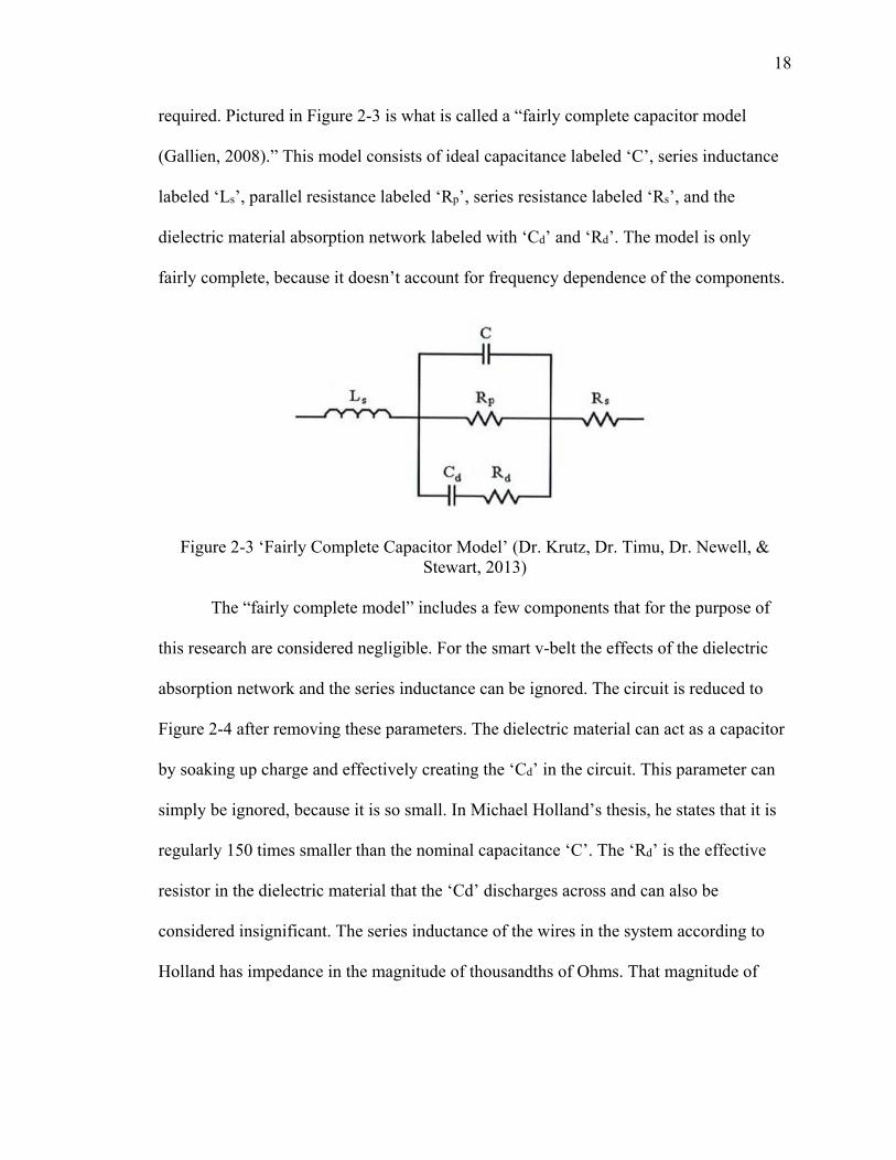
18
required. Pictured in Figure 2-3 is what is called a “fairly complete capacitor model
(Gallien, 2008).” This model consists of ideal capacitance labeled ‘C’, series inductance
labeled ‘Ls’, parallel resistance labeled ‘Rp’, series resistance labeled ‘Rs’, and the
dielectric material absorption network labeled with ‘Cd’ and ‘Rd’. The model is only
fairly complete, because it doesn’t account for frequency dependence of the components.
Figure 2-3 ‘Fairly Complete Capacitor Model’ (Dr. Krutz, Dr. Timu, Dr. Newell, & Stewart, 2013)
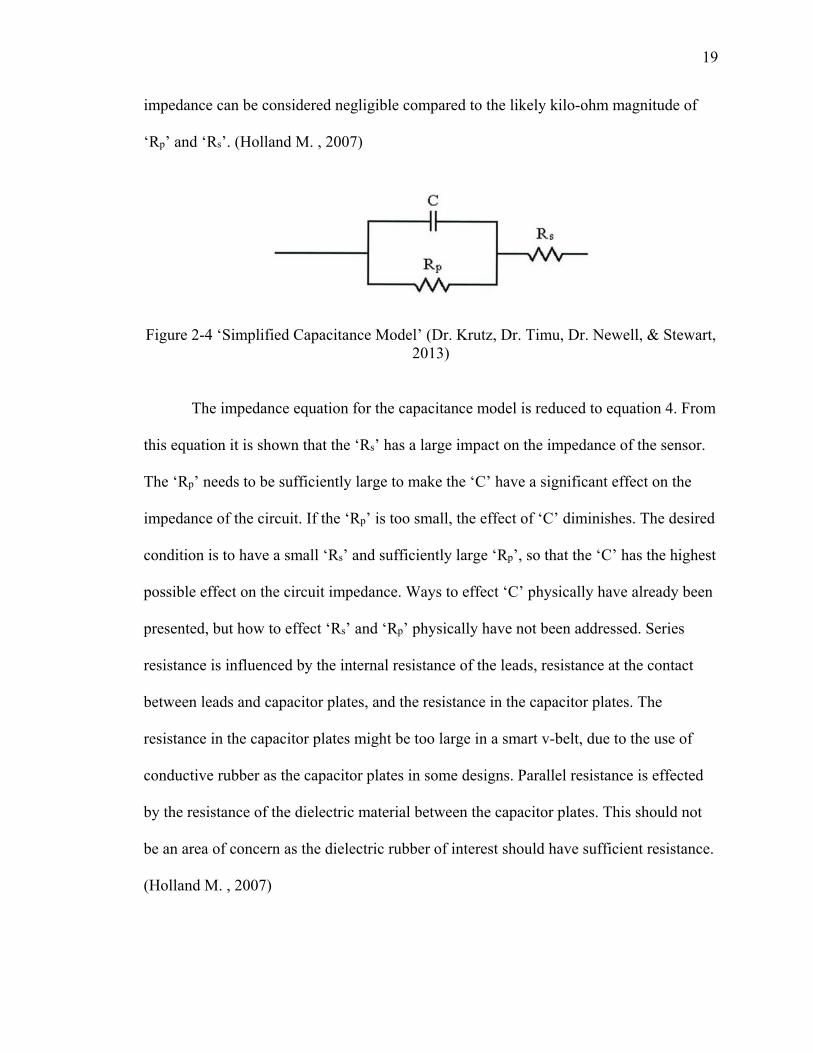
The “fairly complete model” includes a few components that for the purpose of
this research are considered negligible. For the smart v-belt the effects of the dielectric
absorption network and the series inductance can be ignored. The circuit is reduced to
Figure 2-4 after removing these parameters. The dielectric material can act as a capacitor
by soaking up charge and effectively creating the ‘Cd’ in the circuit. This parameter can
simply be ignored, because it is so small. In Michael Holland’s thesis, he states that it is
regularly 150 times smaller than the nominal capacitance ‘C’. The ‘Rd’ is the effective
resistor in the dielectric material that the ‘Cd’ discharges across and can also be
considered insignificant. The series inductance of the wires in the system according to
Holland has impedance in the magnitude of thousandths of Ohms. That magnitude of
19
impedance can be considered negligible compared to the likely kilo-ohm magnitude of
‘Rp’ and ‘Rs’. (Holland M. , 2007)
Figure 2-4 ‘Simplified Capacitance Model’ (Dr. Krutz, Dr. Timu, Dr. Newell, & Stewart, 2013)
The impedance equation for the capacitance model is reduced to equation 4. From
this equation it is shown that the ‘Rs’ has a large impact on the impedance of the sensor.
The ‘Rp’ needs to be sufficiently large to make the ‘C’ have a significant effect on the
impedance of the circuit. If the ‘Rp’ is too small, the effect of ‘C’ diminishes. The desired
condition is to have a small ‘Rs’ and sufficiently large ‘Rp’, so that the ‘C’ has the highest
possible effect on the circuit impedance. Ways to effect ‘C’ physically have already been
presented, but how to effect ‘Rs’ and ‘Rp’ physically have not been addressed. Series
resistance is influenced by the internal resistance of the leads, resistance at the contact
between leads and capacitor plates, and the resistance in the capacitor plates. The
resistance in the capacitor plates might be too large in a smart v-belt, due to the use of
conductive rubber as the capacitor plates in some designs. Parallel resistance is effected
by the resistance of the dielectric material between the capacitor plates. This should not
be an area of concern as the dielectric rubber of interest should have sufficient resistance.
(Holland M. , 2007)
20
| |^
Equation 4 (Holland M. , 2007)
The capacitor model is established above. The data from this model can be sensed
by an LCR meter, but it is not practical for a data acquisition system. The most practical
signal for data acquisition is voltage. Voltage differentials are an easily transferred and
interpreted signal for data acquisition systems. For this reason, the capacitance model
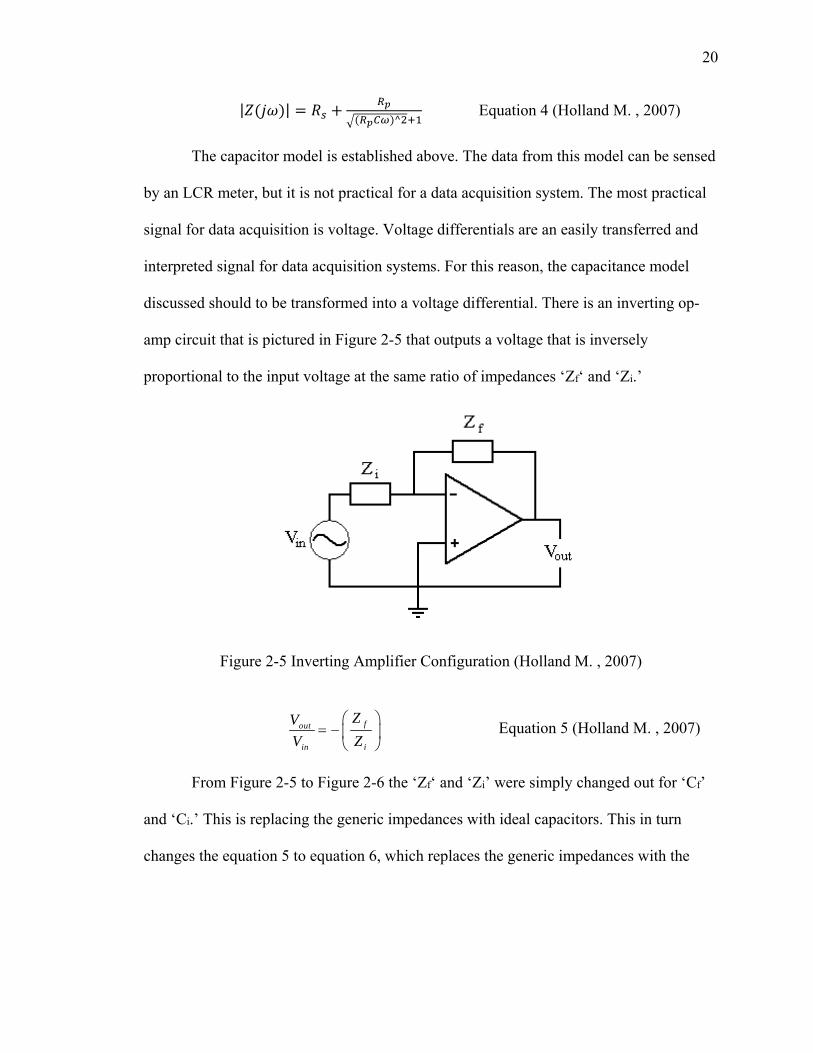
discussed should to be transformed into a voltage differential. There is an inverting op-
amp circuit that is pictured in Figure 2-5 that outputs a voltage that is inversely
proportional to the input voltage at the same ratio of impedances ‘Zf‘ and ‘Zi.’
Figure 2-5 Inverting Amplifier Configuration (Holland M. , 2007)
fout
in i
ZV
V Z
Equation 5 (Holland M. , 2007)
From Figure 2-5 to Figure 2-6 the ‘Zf‘ and ‘Zi’ were simply changed out for ‘Cf’
and ‘Ci.’ This is replacing the generic impedances with ideal capacitors. This in turn
changes the equation 5 to equation 6, which replaces the generic impedances with the
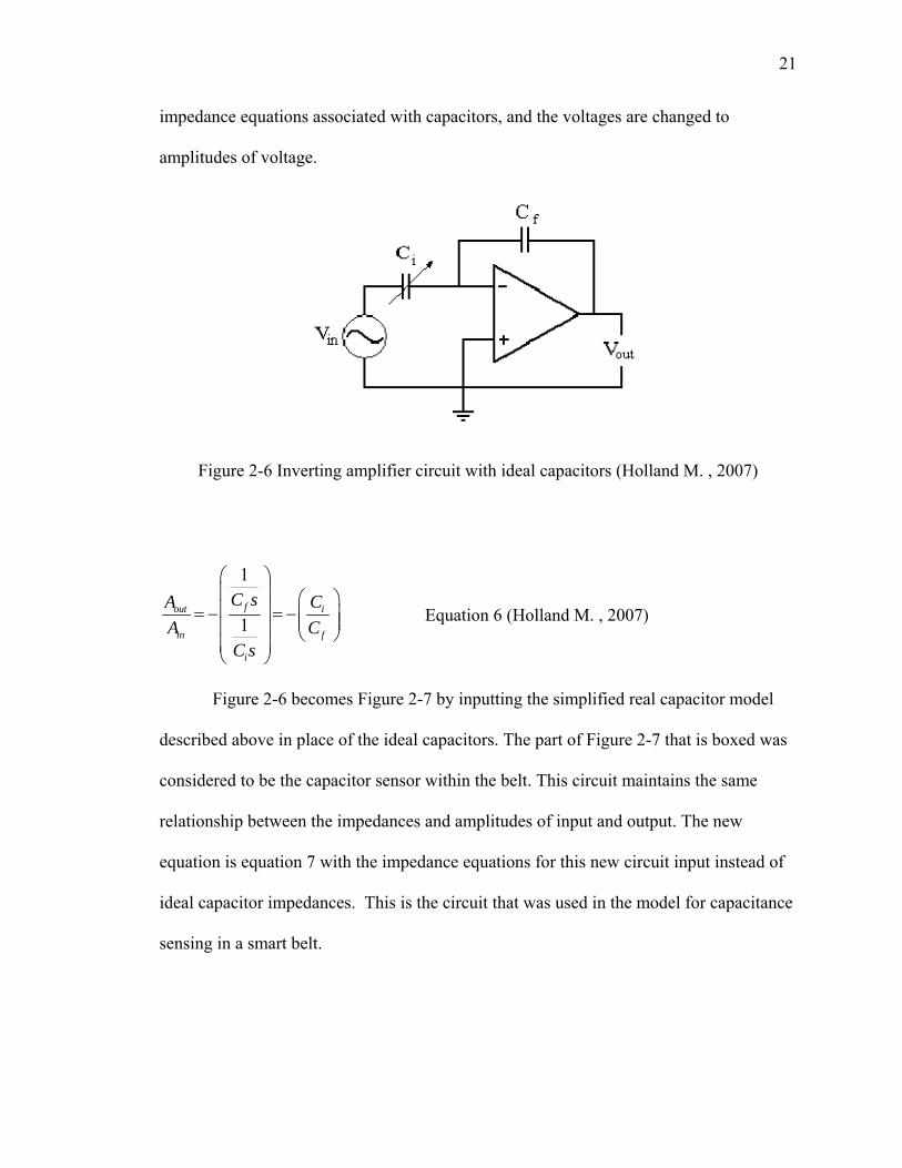
21
impedance equations associated with capacitors, and the voltages are changed to
amplitudes of voltage.
Figure 2-6 Inverting amplifier circuit with ideal capacitors (Holland M. , 2007)
1
1fout i
in f
i
C sA C
A CC s
Equation 6 (Holland M. , 2007)
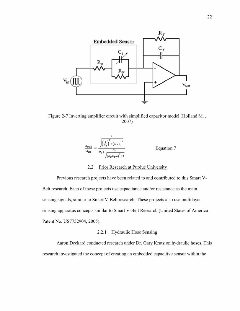
Figure 2-6 becomes Figure 2-7 by inputting the simplified real capacitor model
described above in place of the ideal capacitors. The part of Figure 2-7 that is boxed was
considered to be the capacitor sensor within the belt. This circuit maintains the same
relationship between the impedances and amplitudes of input and output. The new
equation is equation 7 with the impedance equations for this new circuit input instead of
ideal capacitor impedances. This is the circuit that was used in the model for capacitance
sensing in a smart belt.
22
Figure 2-7 Inverting amplifier circuit with simplified capacitor model (Holland M. , 2007)
Equation 7
2.2 Prior Research at Purdue University
Previous research projects have been related to and contributed to this Smart V-
Belt research. Each of these projects use capacitance and/or resistance as the main
sensing signals, similar to Smart V-Belt research. These projects also use multilayer
sensing apparatus concepts similar to Smart V-Belt Research (United States of America
Patent No. US7752904, 2005).
2.2.1 Hydraulic Hose Sensing
Aaron Deckard conducted research under Dr. Gary Krutz on hydraulic hoses. This
research investigated the concept of creating an embedded capacitive sensor within the
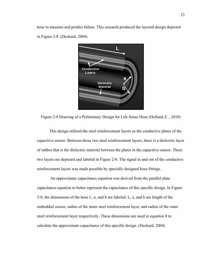
23
hose to measure and predict failure. This research produced the layered design depicted
in Figure 2-8. (Deckard, 2004)
Figure 2-8 Drawing of a Preliminary Design for Life Sense Hose (Holland Z. , 2010)
This design utilized the steel reinforcement layers as the conductive plates of the
capacitive sensor. Between those two steel reinforcement layers, there is a dielectric layer
of rubber that is the dielectric material between the plates in the capacitive sensor. These
two layers are depicted and labeled in Figure 2-8. The signal in and out of the conductive
reinforcement layers was made possible by specially designed hose fittings.
An approximate capacitance equation was derived from the parallel plate
capacitance equation to better represent the capacitance of this specific design. In Figure
2-8, the dimensions of the hose L, a, and b are labeled. L, a, and b are length of the
embedded sensor, radius of the inner steel reinforcement layer, and radius of the outer
steel reinforcement layer respectively. These dimensions are used in equation 8 to
calculate the approximate capacitance of this specific design. (Deckard, 2004)
b
aDielectric Mater ial
Conductive Layers
L

24
Equation 8
With this proposed design and model equation for capacitance, there were
assumptions made about what would change the capacitance measurements. It was
assumed that degradation of either of the steel reinforcement layers would effectively
affect the L, a, and/or b values changing capacitance. Another assumption was that
degradation of the dielectric layer would effectively affect the value and/or the
relationship between a and b changing the capacitance.
Figure 2-9 shows the relationship between capacitance readings from the
embedded sensor in relation to the pressure of the oil within the hose. These results show
slight change in capacitance readings associated with the loading and unloading of the
hose; about 2% change. With this creep and the pressure range in mind, a capacitance
threshold can be established for a maximum pressure the hose can be exposed to before
needing to be replaced. (Deckard, 2004)
Figure 2-9 Experimental Capacitance and static pressure relationship (Deckard, 2004)
25
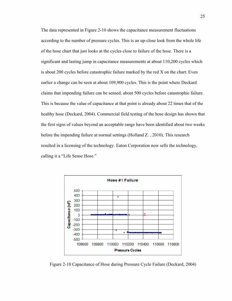
The data represented in Figure 2-10 shows the capacitance measurement fluctuations
according to the number of pressure cycles. This is an up-close look from the whole life
of the hose chart that just looks at the cycles close to failure of the hose. There is a
significant and lasting jump in capacitance measurements at about 110,200 cycles which
is about 200 cycles before catastrophic failure marked by the red X on the chart. Even
earlier a change can be seen at about 109,900 cycles. This is the point where Deckard
claims that impending failure can be sensed, about 500 cycles before catastrophic failure.
This is because the value of capacitance at that point is already about 22 times that of the
healthy hose (Deckard, 2004). Commercial field testing of the hose design has shown that
the first signs of values beyond an acceptable range have been identified about two weeks
before the impending failure at normal settings (Holland Z. , 2010). This research
resulted in a licensing of the technology. Eaton Corporation now sells the technology,
calling it a “Life Sense Hose.”
Figure 2-10 Capacitance of Hose during Pressure Cycle Failure (Deckard, 2004)
26
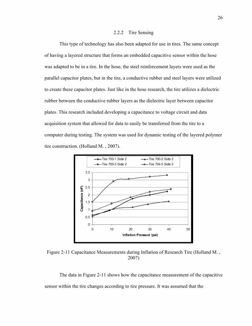
2.2.2 Tire Sensing
This type of technology has also been adapted for use in tires. The same concept
of having a layered structure that forms an embedded capacitive sensor within the hose
was adapted to be in a tire. In the hose, the steel reinforcement layers were used as the
parallel capacitor plates, but in the tire, a conductive rubber and steel layers were utilized
to create these capacitor plates. Just like in the hose research, the tire utilizes a dielectric
rubber between the conductive rubber layers as the dielectric layer between capacitor
plates. This research included developing a capacitance to voltage circuit and data
acquisition system that allowed for data to easily be transferred from the tire to a
computer during testing. The system was used for dynamic testing of the layered polymer
tire construction. (Holland M. , 2007).
Figure 2-11 Capacitance Measurements during Inflation of Research Tire (Holland M. , 2007)
The data in Figure 2-11 shows how the capacitance measurement of the capacitive
sensor within the tire changes according to tire pressure. It was assumed that the
27
capacitance would change according to inflation pressure, but the amount that it changed
was not expected. The expected change was supposed to only be due to a slight change in
distance between plates. The hypothesized reason for the larger change was due to a
decrease in the parallel resistance as tire pressure rises. Lower parallel resistance
typically causes an increase in capacitance.
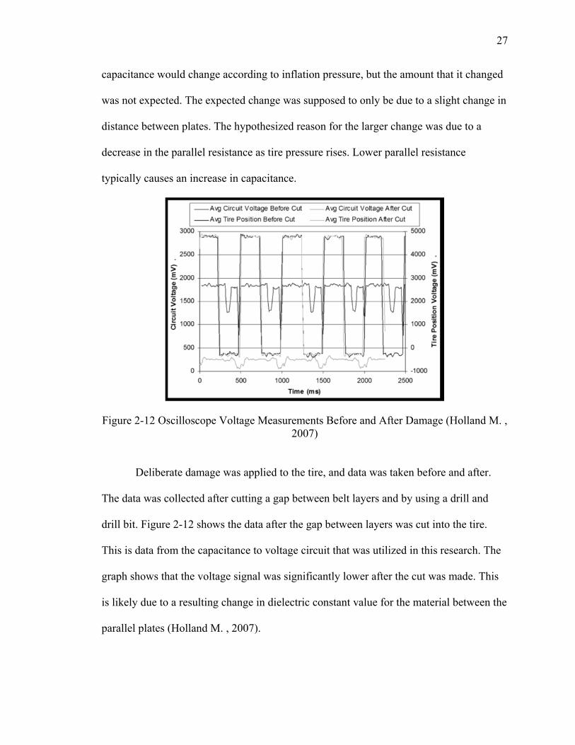
Figure 2-12 Oscilloscope Voltage Measurements Before and After Damage (Holland M. , 2007)
Deliberate damage was applied to the tire, and data was taken before and after.
The data was collected after cutting a gap between belt layers and by using a drill and
drill bit. Figure 2-12 shows the data after the gap between layers was cut into the tire.
This is data from the capacitance to voltage circuit that was utilized in this research. The
graph shows that the voltage signal was significantly lower after the cut was made. This
is likely due to a resulting change in dielectric constant value for the material between the
parallel plates (Holland M. , 2007).
28
2.2.3 Hydraulic O-Ring Seals
The hydraulic O-ring seal research took the embedded capacitive sensor
technology and applied it to a much smaller structure with different failure modes
compared to the previous technologies it had been applied. The small size, and therefore
thin layers of the layered polymer structure, made the construction of the embedded
sensor in the O-ring more difficult. The initial method was a five part layered structure
with common rubber on the top and bottom, a layer of
hexaflouropropylenevinylideneflouride copolymer (FKM) in the middle, and two copper
foil or brass mesh layers sandwiched between the other three layers. Bonding of these
layers proved to be the most difficult step of the construction. Mechanical and chemical
methods of bonding were attempted. Each of the iterations couldn’t establish proper
adhesion, which caused the dielectric layer became distorted. Electrical shorts occurred
due to this distortion. The final prototype design used conductive silicone layers as the
capacitor plates. The dielectric and conductive layers were molded separately and then
bonded together in a subsequent process. The final prototypes were provided by Parker
Hannifin (Gallien, 2008).
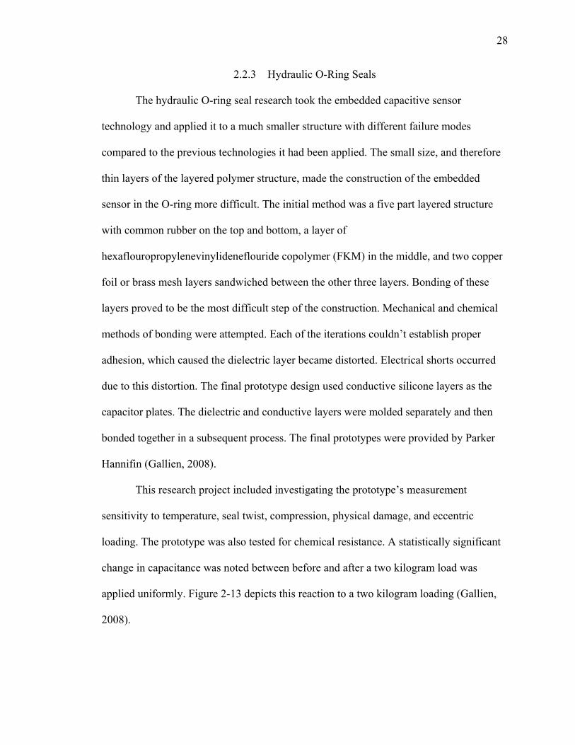
This research project included investigating the prototype’s measurement
sensitivity to temperature, seal twist, compression, physical damage, and eccentric
loading. The prototype was also tested for chemical resistance. A statistically significant
change in capacitance was noted between before and after a two kilogram load was
applied uniformly. Figure 2-13 depicts this reaction to a two kilogram loading (Gallien,
2008).
29
Figure 2-13 Load Test of Research O-Rings BI10 and BJ10 (Gallien, 2008)
The sensor was shown to have a slightly positive linear trend in the capacitance
reading vs. time as the O-ring was heated to 450 Degrees Fahrenheit. The changes in
measurement due to damages are depicted in Figure 2-14. The damages created
significant changes in measurements, but the trends were difficult to see or predict. The
first abrasion increased the capacitance relative to baseline, and confusingly, the second
abrasion decreased capacitance relative to the baseline. The cuts and punctures created
the largest changes in capacitance. It can be seen that the values have drift over time
which were hypothesized to be due to material creep. This research concluded that this is
a viable technology. The sensor was able to detect changes in capacitance due to
compression, physical damage, and temperature. The technology needed to be researched
further to discover optimal material and set-up for greater reliability. Research to
establish reliability, calibration, and failure cut-off need to be conducted in the future.
22.00
22.20
22.40
22.60
22.80
23.00
0 500 1000 1500 2000
Time (seconds)
Cap
acit
ance
(p
F) BI10
BJ10
BI10 - 3 Sigma
BI10 + 3 Sigma
BI10 - 3 Sigma
BJ10 + 3 Sigma

30
Figure 2-14 Capacitance Measurements Before and After Specific Damages (Gallien, 2008)
2.2.4 Lumbar Disc Replacement
Alyssa Brune researched the application of the imbedded capacitive sensor
technology to artificial lumbar disc replacements. The main failure mode of the lumbar
disc replacements was known to be the degradation due to wear of the ultra-high
molecular weight polyethylene layer. Prior to her research, the only way to detect this
wear was for the patient to experience pain and bring that to their doctor’s attention. A
model of the special polyethylene was tested by various wear and failure modes to
determine the viability of the technology. (Brune, 2009)
In the replacement the metal alloy section of the disc continually rubs on the
polyethylene layer creating a worn trough in the material. This type of wear was
simulated by repeatedly scraping a screwdriver over the material creating a similar effect.
The capacitance was read in stages based on progressively the more and more
pronounced the trough became in the material. A final testing stage was measured after a
31
separate trough was inflicted parallel to the first. The capacitance readings had and
overall increasing trend with increasing wear on the material. There was also a change in
capacitance detected due to loading on the material. Since the changes in capacitance
could be detected in these conditions, the concept was considered viable. (Brune, 2009)
2.3 Current Belt Sensing Technologies in Industry
Many older methods have been used to monitor belts, but new methods are being
developed all of the time. The demand for a practical and accurate sensing method has
been considered a significant enough to call many companies to research the topic. A
small selection of the industry’s research and current products in the area is presented
below.
2.3.1 SensSystems
This system monitors only the amount of slippage the belt is experiencing. This is
because the major assumption for this research was that a primary failure mode of v-belts
is caused by slippage. Loss of consistent power is another major reason for belt slip
monitoring systems. (Brown, 2012)
The SenSystems belt slip monitoring system is based on the assumptions of
Equation 9. This is the equation that is true under the zero slip condition. The system
monitors this equation. When the equation is not equal to zero, there is slip. This means
for a real belt and pulley system, it will not be equal to zero, because there is nearly
always some slip. When this equation gets a certain distance from being equal to zero, the
system knows there is too much slip and will alert the user.
Equation 9
32
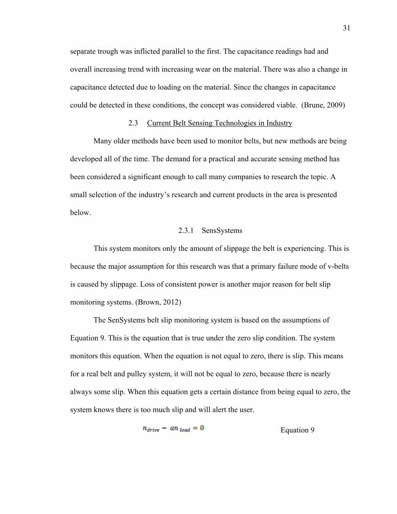
Figure 2-15 below shows both the diagram and photograph of the monitoring
system. The sensors determine the radial speed of the loaded pulley and driven pulley and
then the computer automatically and continually checks the equation for slip amount. The
relationship monitored was the difference from zero that Equation 9 equals. Equation 10
was developed to better represent slip and give an easier number to monitor. When slip is
between 1.5-3 percent, the system is considered to need maintenance. When slip is between
3-4.5 percent, the system is considered to urgently need maintenance and that belt breakage
is possible (Brown, 2012).
Equation 10
Figure 2-15 Diagram (left) and Photograph (right) of the slip monitoring system (Brown, 2012)
33
2.3.2 Schrader
Schrader Electronics sells a belt monitoring system that monitors slip. Schrader
does not give much information on the specifics of how the system works. The system is
said to measure belt slip and wear. The system uses non-intrusive sensors attached to the
pulleys and is effective up to 8000 rpm. It has a wireless or USB data transfer
capabilities. The data management system has a three year battery life. (Electronics,
n.d.).
2.3.3 Tele Haase
Tele Haase Has a V-belt Monitoring system that monitors slippage and breakage,
product G2CM400V10AL20. Tele uses what they call a Power Factor Meter to monitor
the belt. Tele promotes that the system gives early detection and prevention of belt
system downtime and motor protection. They also claim that the system is easy to set up
and low cost (Tele, n.d.).
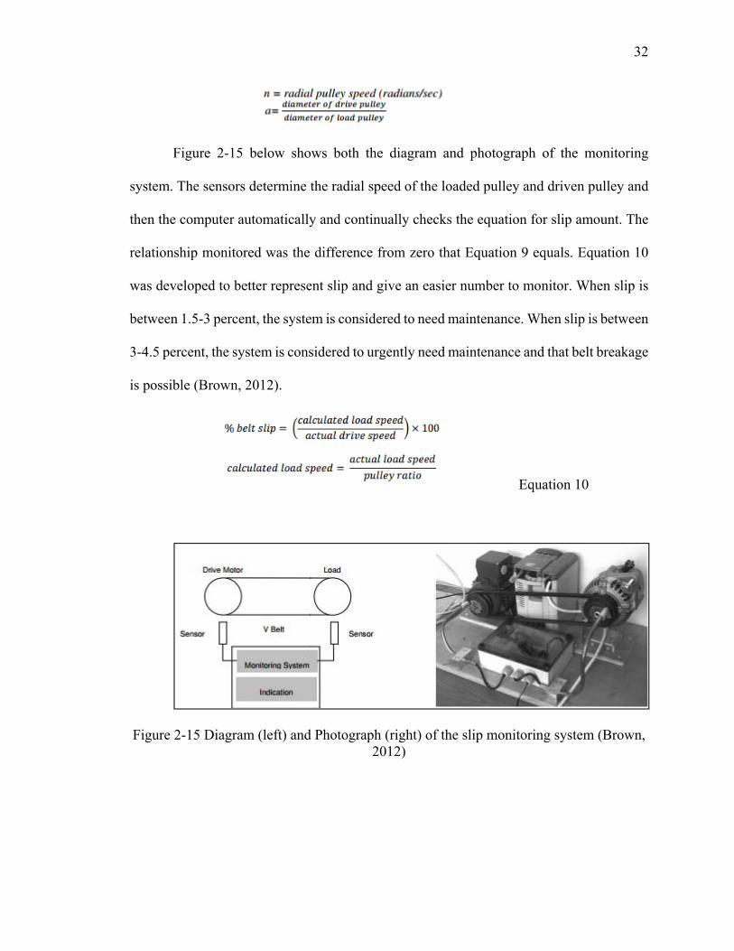
2.3.4 Honeywell
Honeywell has developed a belt monitoring system called Belt Asset Inspection
System or BeltAIS. Honeywell developed a high speed and resolution camera that can
withstand harsh environments for this system. This system uses real-time video-based
inspection of the belt. Honeywell has developed algorithms to turn the video feed into
usable data. This data is analyzed and compared to a vast database of damage data points
that indicate defect location, category, and intensity. This system has been adapted for
just conveyor belts. Figure 2-16 depicts a possible configuration of the system. In this
drawing, other Honeywell as well, as third party monitoring products, are included.
(Honeywell, 2012).
34
Figure 2-16 Drawing of possible BeltAIS configuration (Honeywell, 2012).
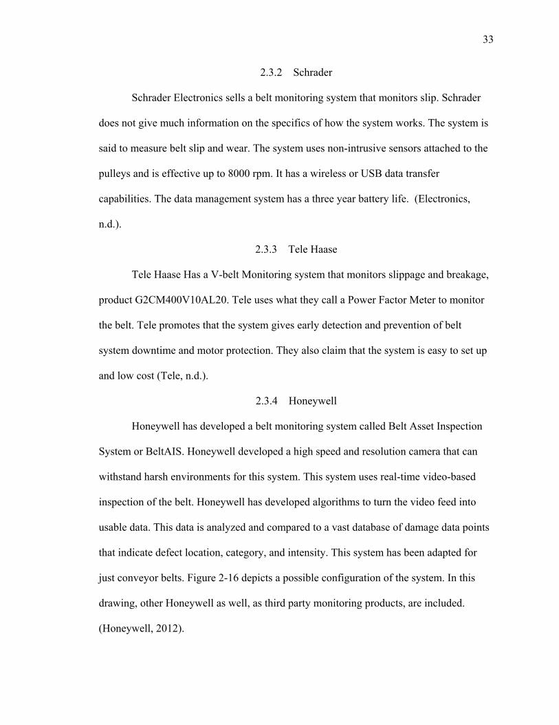
2.3.5 Bridgestone
Bridgestone has a belt monitoring system that they call Monitrix. The Monitrix
system mainly monitors the belt’s thickness. Monitrix utilizes an embedded sensor to
monitor thickness. The embedded sensors are read by a stationary detecting device. This
is a very simple monitoring system. This is a new technology for Bridgestone, and the
specifics of it have not been released. In Figure 2-17, the system is depicted. The
embedded sensor in the figure looks like a layered structure. (Bridgestone, 2015).

35
Figure 2-17 Drawing of Bridgestone’s Monitrix System (Bridgestone, 2015)
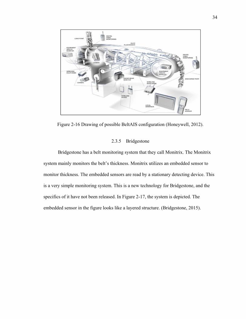
2.3.6 Continental Contitech
Continental Contitech was the re-branding of what was Goodyear Veyance
Division. Contitech’s monitoring system has five different parameters that are analyzed.
The system has multiple different embedded loop sensors. These sensor loops are broken,
when there is a rip in the belt, and the system knows to shut down. Another embedded
sensor detects the elongation of the splice in the belt. With each of these embedded
sensors RFID technology has been utilized to tag and track the specific embedded sensor
that has been tripped. This is a section of common failure in a conveyor belt. An external
sensor detects belt thickness in areas where wear normally takes place. From historical
data, a certain thickness will alert the user that the belt needs to be changed. The system
also has a visual monitor using laser technology to generate a digital image of the belt
from which damages can be detected. Lastly, the system has an external monitor that
36
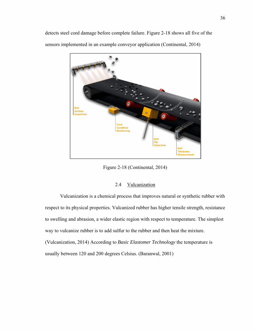
detects steel cord damage before complete failure. Figure 2-18 shows all five of the
sensors implemented in an example conveyor application (Continental, 2014)
Figure 2-18 (Continental, 2014)
2.4 Vulcanization
Vulcanization is a chemical process that improves natural or synthetic rubber with
respect to its physical properties. Vulcanized rubber has higher tensile strength, resistance
to swelling and abrasion, a wider elastic region with respect to temperature. The simplest
way to vulcanize rubber is to add sulfur to the rubber and then heat the mixture.
(Vulcanization, 2014) According to Basic Elastomer Technology the temperature is
usually between 120 and 200 degrees Celsius. (Baranwal, 2001)
37
CHAPTER 3. SMART V-BELT DESIGN CONCEPTS
The designs proposed for the sensing system in V-Belts are largely based on prior
research at Purdue University. Specifically, the choice of using dielectric and conductive
rubbers to form an embedded pseudo capacitor or capacitive sensor was based on
previous research conducted under Dr. Gary Krutz. These prior research topics adapted
this concept to many other types of polymer products.
3.1 V-Belt Design Concepts
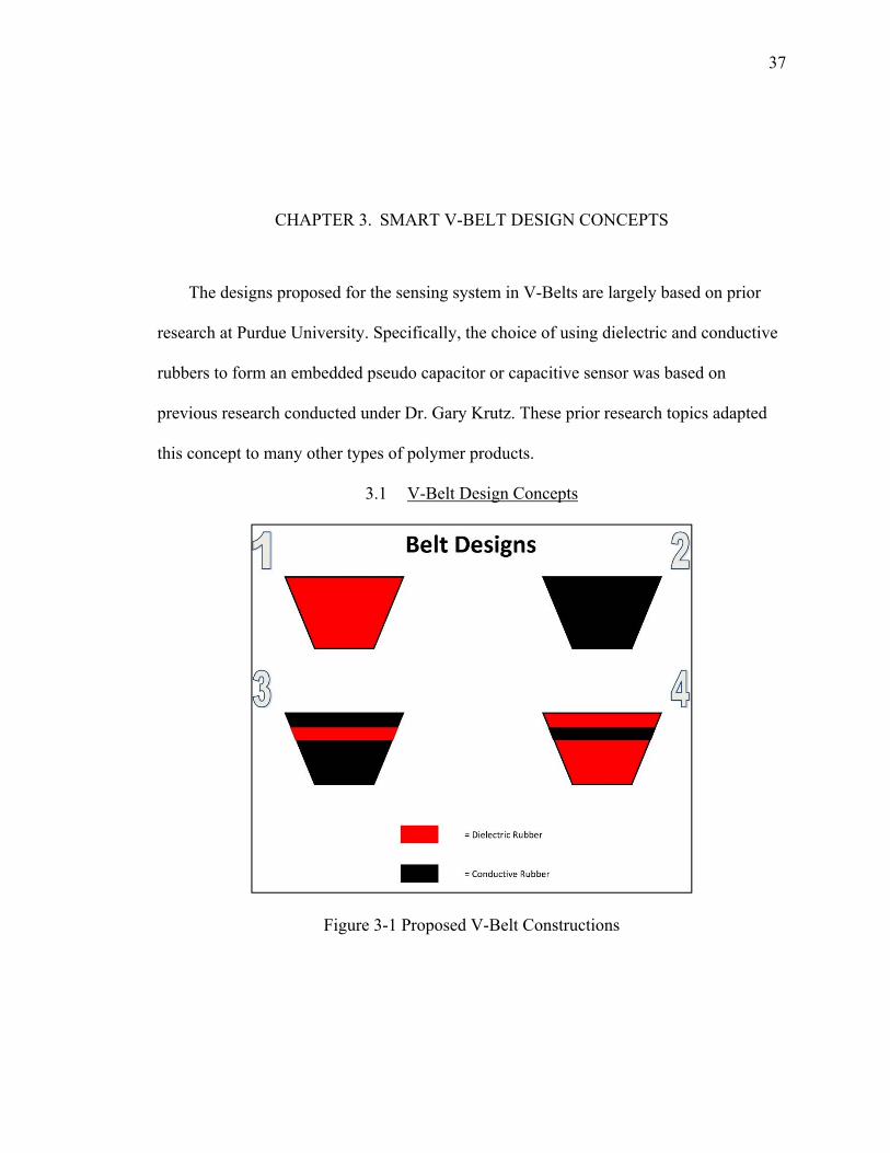
Figure 3-1 Proposed V-Belt Constructions

38
Depicted in Figure 3-1 are the four possible belt cross-sectional designs for this
Smart V-Belt research. The first design is a fully dielectric rubber belt. The whole belt is
the dielectric layer of the pseudo-capacitor that is the sensor with this design. The sheave
and/or idler pulley act as the capacitor plates in this design. The second design is a fully
conductive rubber belt. This design could test the sensitivity of resistance through the belt
to damage. The third belt is a belt with a conductive layer on top, a dielectric layer in the
tension cord region, and a conductive layer on the bottom. This belt has all of the
components of the pseudo-capacitor built in. This means the main region that the sensing
will give information on is the tension cord region. The fourth design is a belt with a top
layer of dielectric rubber, a layer of conductive rubber in the tension cord region, and a
bottom layer of dielectric rubber. This design has the capacitor plate and dielectric layer
built in. The sheave or tensioner pulley acts as the capacitor plates to complete the
pseudo-capacitor sensor. The bottom dielectric layer or top dielectric layer can be the
region of focus for sensing. More design ideas that were discussed early in the research
are shown in the appendix.
3.2 Sheave Design Concepts
A nontrivial aspect of this research was designing the system to deliver the signal
to and from the embedded capacitive sensor in the belt. The design needed to be able to
read across the belt in a way that would contact one of the capacitor plates at a time. The
signal needed to be read through a significant section of belt to ensure the reading was
not skewed due to a short signal path bypassing the damage. Each of these sheave designs
utilize one or more slip rings to transmit signal from the spinning copper tape to a
stationary data acquisition system.
39
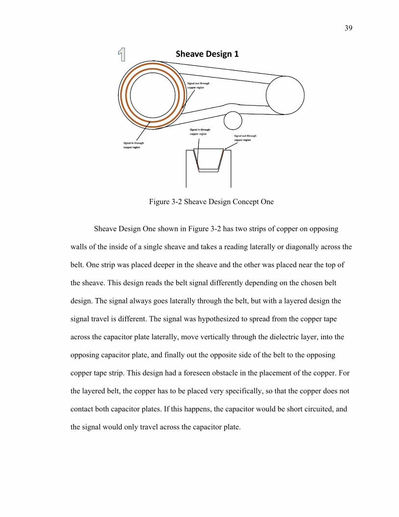
Figure 3-2 Sheave Design Concept One
Sheave Design One shown in Figure 3-2 has two strips of copper on opposing
walls of the inside of a single sheave and takes a reading laterally or diagonally across the
belt. One strip was placed deeper in the sheave and the other was placed near the top of
the sheave. This design reads the belt signal differently depending on the chosen belt
design. The signal always goes laterally through the belt, but with a layered design the
signal travel is different. The signal was hypothesized to spread from the copper tape
across the capacitor plate laterally, move vertically through the dielectric layer, into the
opposing capacitor plate, and finally out the opposite side of the belt to the opposing
copper tape strip. This design had a foreseen obstacle in the placement of the copper. For
the layered belt, the copper has to be placed very specifically, so that the copper does not
contact both capacitor plates. If this happens, the capacitor would be short circuited, and
the signal would only travel across the capacitor plate.
40
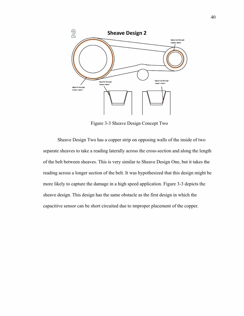
Figure 3-3 Sheave Design Concept Two
Sheave Design Two has a copper strip on opposing walls of the inside of two
separate sheaves to take a reading laterally across the cross-section and along the length
of the belt between sheaves. This is very similar to Sheave Design One, but it takes the
reading across a longer section of the belt. It was hypothesized that this design might be
more likely to capture the damage in a high speed application. Figure 3-3 depicts the
sheave design. This design has the same obstacle as the first design in which the
capacitive sensor can be short circuited due to improper placement of the copper.
41
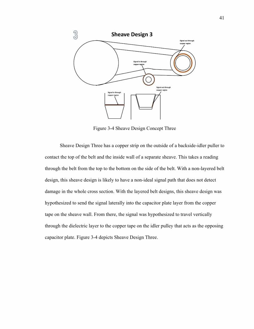
Figure 3-4 Sheave Design Concept Three
Sheave Design Three has a copper strip on the outside of a backside-idler puller to
contact the top of the belt and the inside wall of a separate sheave. This takes a reading
through the belt from the top to the bottom on the side of the belt. With a non-layered belt
design, this sheave design is likely to have a non-ideal signal path that does not detect
damage in the whole cross section. With the layered belt designs, this sheave design was
hypothesized to send the signal laterally into the capacitor plate layer from the copper
tape on the sheave wall. From there, the signal was hypothesized to travel vertically
through the dielectric layer to the copper tape on the idler pulley that acts as the opposing
capacitor plate. Figure 3-4 depicts Sheave Design Three.
42
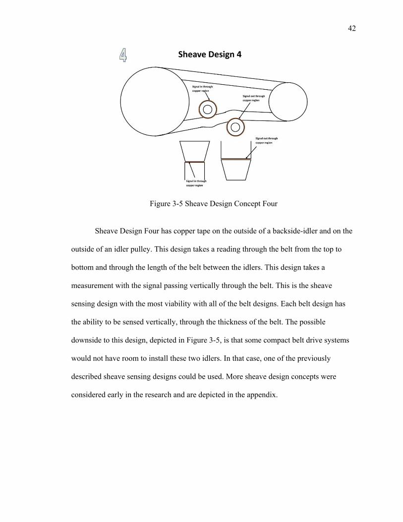
Figure 3-5 Sheave Design Concept Four
Sheave Design Four has copper tape on the outside of a backside-idler and on the
outside of an idler pulley. This design takes a reading through the belt from the top to
bottom and through the length of the belt between the idlers. This design takes a
measurement with the signal passing vertically through the belt. This is the sheave
sensing design with the most viability with all of the belt designs. Each belt design has
the ability to be sensed vertically, through the thickness of the belt. The possible
downside to this design, depicted in Figure 3-5, is that some compact belt drive systems
would not have room to install these two idlers. In that case, one of the previously
described sheave sensing designs could be used. More sheave design concepts were
considered early in the research and are depicted in the appendix.
43
CHAPTER 4. INSTRUMENTATION AND PROCEDURES
4.1 Instrumentation
4.1.1 Belt Making Instruments
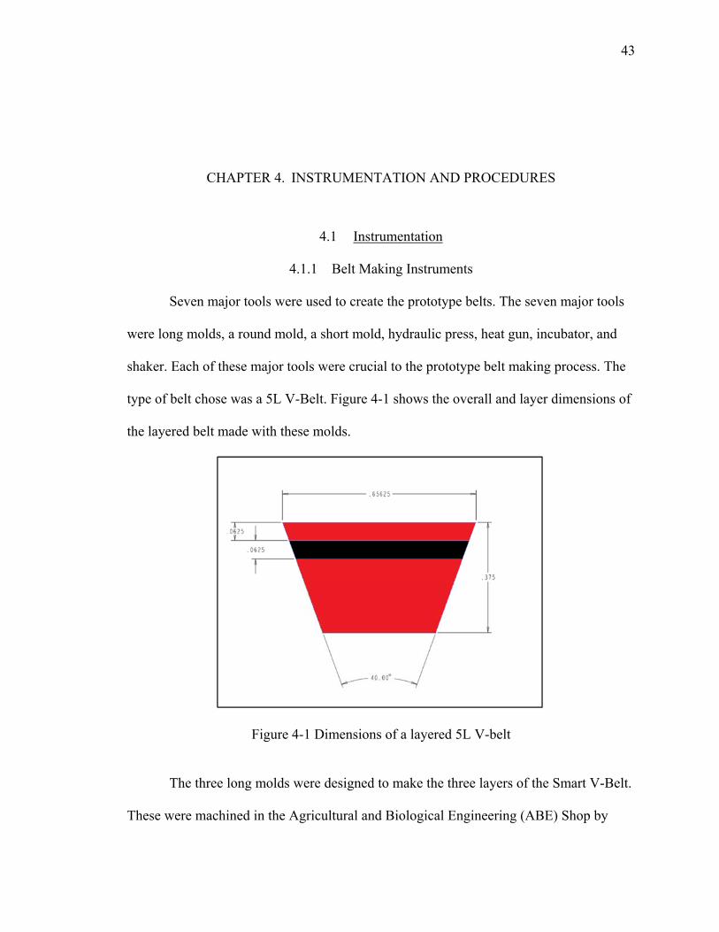
Seven major tools were used to create the prototype belts. The seven major tools
were long molds, a round mold, a short mold, hydraulic press, heat gun, incubator, and
shaker. Each of these major tools were crucial to the prototype belt making process. The
type of belt chose was a 5L V-Belt. Figure 4-1 shows the overall and layer dimensions of
the layered belt made with these molds.
Figure 4-1 Dimensions of a layered 5L V-belt
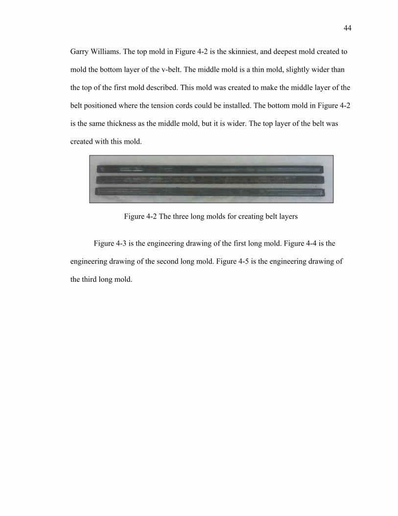
The three long molds were designed to make the three layers of the Smart V-Belt.
These were machined in the Agricultural and Biological Engineering (ABE) Shop by
44
Garry Williams. The top mold in Figure 4-2 is the skinniest, and deepest mold created to
mold the bottom layer of the v-belt. The middle mold is a thin mold, slightly wider than
the top of the first mold described. This mold was created to make the middle layer of the
belt positioned where the tension cords could be installed. The bottom mold in Figure 4-2
is the same thickness as the middle mold, but it is wider. The top layer of the belt was
created with this mold.
Figure 4-2 The three long molds for creating belt layers
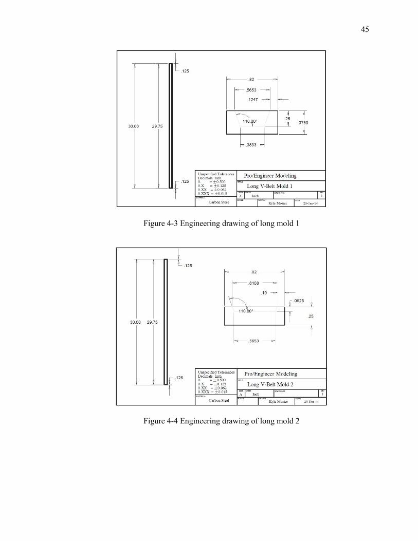
Figure 4-3 is the engineering drawing of the first long mold. Figure 4-4 is the
engineering drawing of the second long mold. Figure 4-5 is the engineering drawing of
the third long mold.
45
Figure 4-3 Engineering drawing of long mold 1
Figure 4-4 Engineering drawing of long mold 2
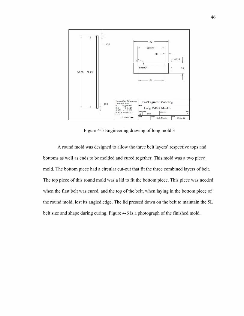
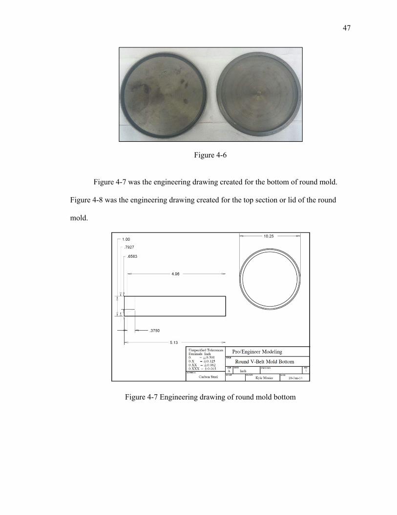
46
Figure 4-5 Engineering drawing of long mold 3
A round mold was designed to allow the three belt layers’ respective tops and
bottoms as well as ends to be molded and cured together. This mold was a two piece
mold. The bottom piece had a circular cut-out that fit the three combined layers of belt.
The top piece of this round mold was a lid to fit the bottom piece. This piece was needed
when the first belt was cured, and the top of the belt, when laying in the bottom piece of
the round mold, lost its angled edge. The lid pressed down on the belt to maintain the 5L
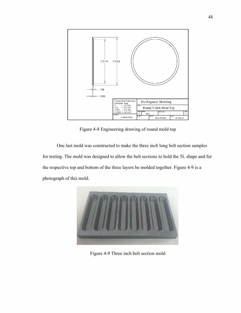
belt size and shape during curing. Figure 4-6 is a photograph of the finished mold.
47
Figure 4-6
Figure 4-7 was the engineering drawing created for the bottom of round mold.
Figure 4-8 was the engineering drawing created for the top section or lid of the round
mold.
Figure 4-7 Engineering drawing of round mold bottom
48
Figure 4-8 Engineering drawing of round mold top
One last mold was constructed to make the three inch long belt section samples
for testing. The mold was designed to allow the belt sections to hold the 5L shape and for
the respective top and bottom of the three layers be molded together. Figure 4-9 is a
photograph of this mold.
Figure 4-9 Three inch belt section mold
49
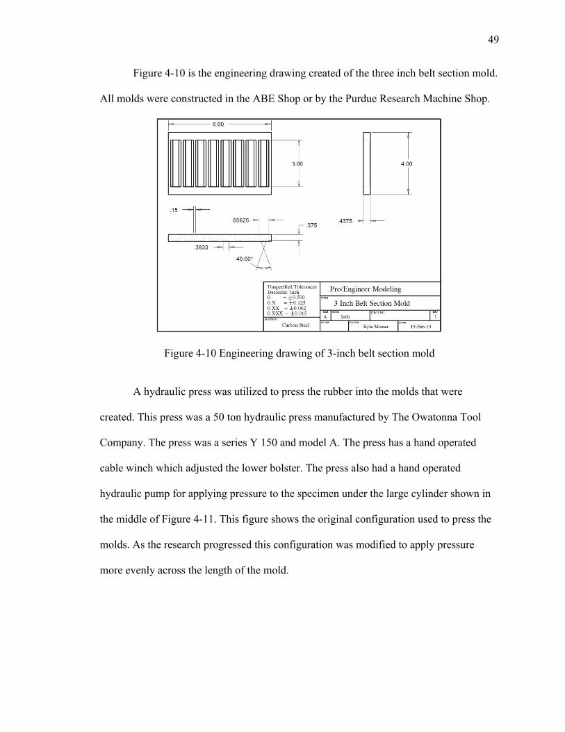
Figure 4-10 is the engineering drawing created of the three inch belt section mold.
All molds were constructed in the ABE Shop or by the Purdue Research Machine Shop.
Figure 4-10 Engineering drawing of 3-inch belt section mold
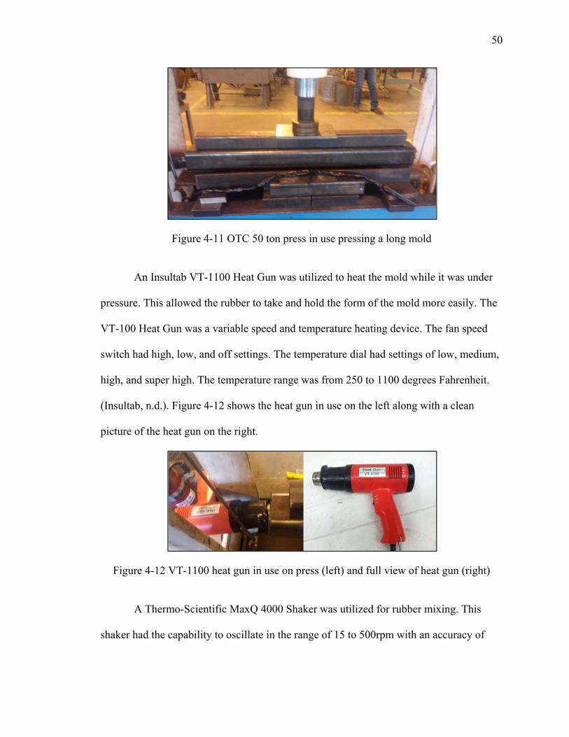
A hydraulic press was utilized to press the rubber into the molds that were
created. This press was a 50 ton hydraulic press manufactured by The Owatonna Tool
Company. The press was a series Y 150 and model A. The press has a hand operated
cable winch which adjusted the lower bolster. The press also had a hand operated
hydraulic pump for applying pressure to the specimen under the large cylinder shown in
the middle of Figure 4-11. This figure shows the original configuration used to press the
molds. As the research progressed this configuration was modified to apply pressure
more evenly across the length of the mold.
50
Figure 4-11 OTC 50 ton press in use pressing a long mold
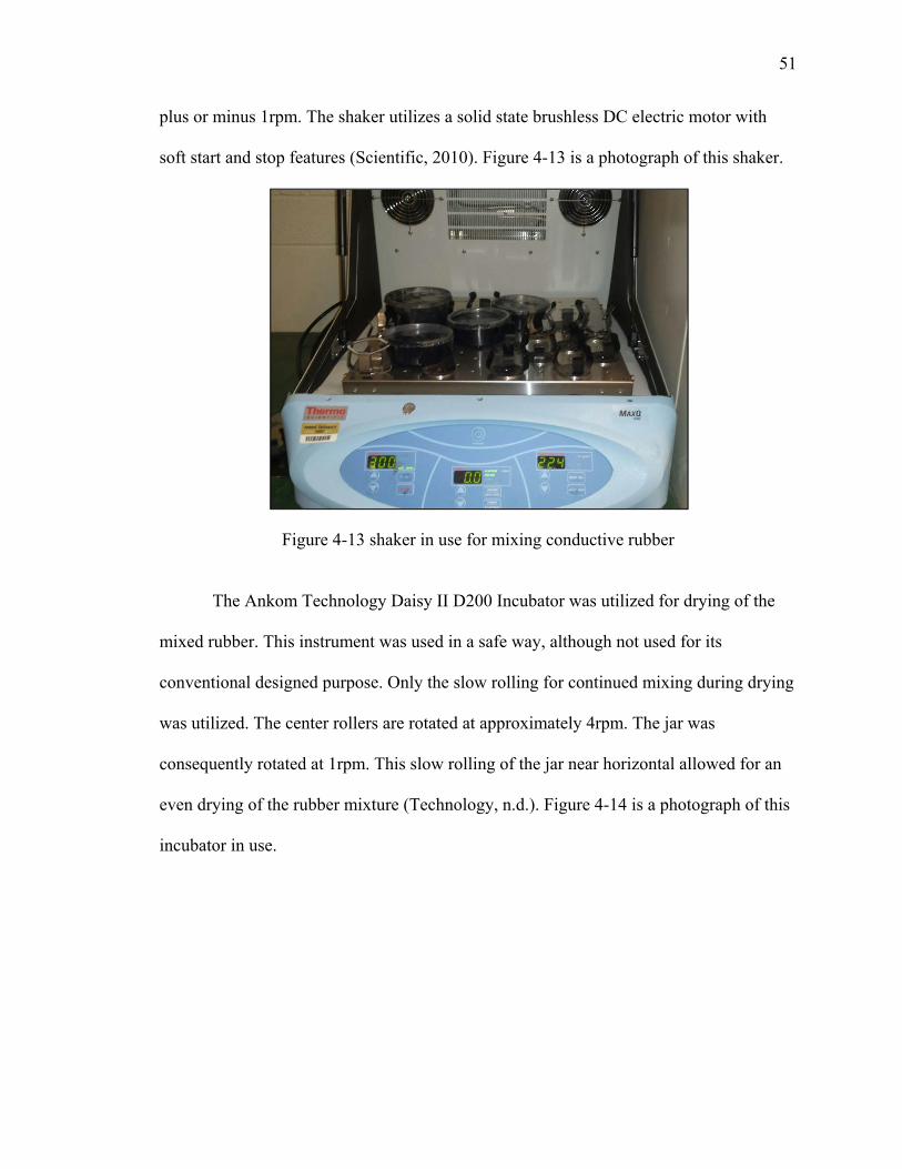
An Insultab VT-1100 Heat Gun was utilized to heat the mold while it was under
pressure. This allowed the rubber to take and hold the form of the mold more easily. The
VT-100 Heat Gun was a variable speed and temperature heating device. The fan speed
switch had high, low, and off settings. The temperature dial had settings of low, medium,
high, and super high. The temperature range was from 250 to 1100 degrees Fahrenheit.
(Insultab, n.d.). Figure 4-12 shows the heat gun in use on the left along with a clean
picture of the heat gun on the right.
Figure 4-12 VT-1100 heat gun in use on press (left) and full view of heat gun (right)
A Thermo-Scientific MaxQ 4000 Shaker was utilized for rubber mixing. This
shaker had the capability to oscillate in the range of 15 to 500rpm with an accuracy of
51
plus or minus 1rpm. The shaker utilizes a solid state brushless DC electric motor with
soft start and stop features (Scientific, 2010). Figure 4-13 is a photograph of this shaker.
Figure 4-13 shaker in use for mixing conductive rubber
The Ankom Technology Daisy II D200 Incubator was utilized for drying of the
mixed rubber. This instrument was used in a safe way, although not used for its
conventional designed purpose. Only the slow rolling for continued mixing during drying
was utilized. The center rollers are rotated at approximately 4rpm. The jar was
consequently rotated at 1rpm. This slow rolling of the jar near horizontal allowed for an
even drying of the rubber mixture (Technology, n.d.). Figure 4-14 is a photograph of this
incubator in use.
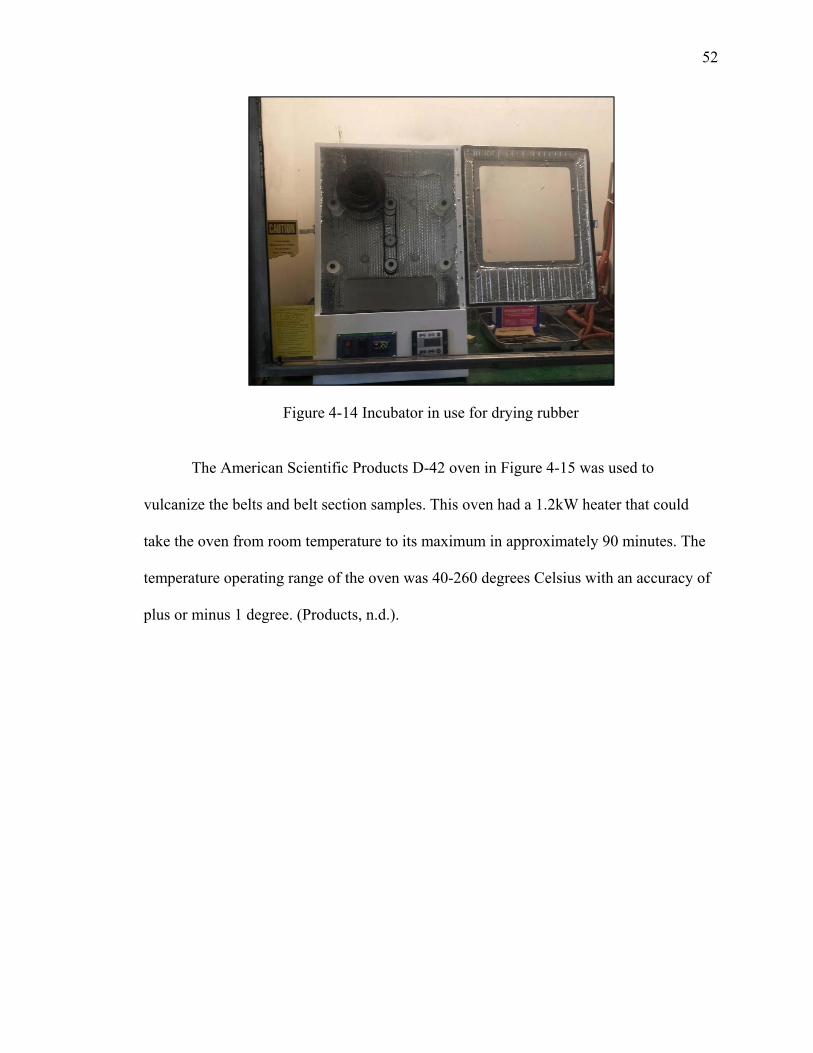
52
Figure 4-14 Incubator in use for drying rubber
The American Scientific Products D-42 oven in Figure 4-15 was used to
vulcanize the belts and belt section samples. This oven had a 1.2kW heater that could
take the oven from room temperature to its maximum in approximately 90 minutes. The
temperature operating range of the oven was 40-260 degrees Celsius with an accuracy of
plus or minus 1 degree. (Products, n.d.).
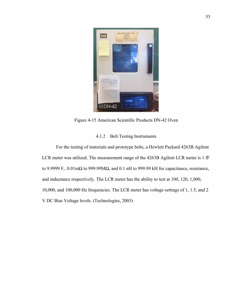
53
Figure 4-15 American Scientific Products DN-42 Oven
4.1.2 Belt Testing Instruments
For the testing of materials and prototype belts, a Hewlett Packard 4263B Agilent
LCR meter was utilized. The measurement range of the 4263B Agilent LCR meter is 1 fF
to 9.9999 F, .0.01mΩ to 999.99MΩ, and 0.1 nH to 999.99 kH for capacitance, resistance,
and inductance respectively. The LCR meter has the ability to test at 100, 120, 1,000,
10,000, and 100,000 Hz frequencies. The LCR meter has voltage settings of 1, 1.5, and 2
V DC Bias Voltage levels. (Technologies, 2003)
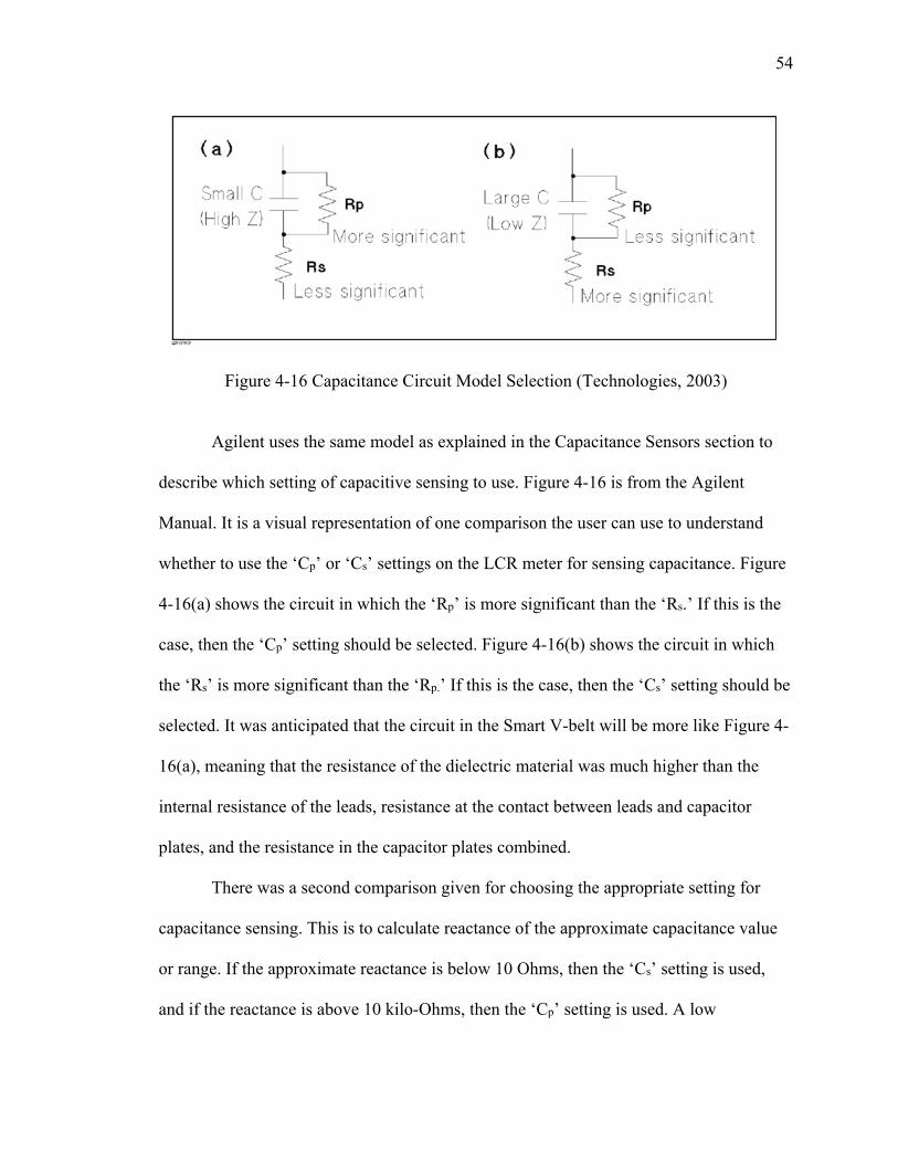
54
Figure 4-16 Capacitance Circuit Model Selection (Technologies, 2003)
Agilent uses the same model as explained in the Capacitance Sensors section to
describe which setting of capacitive sensing to use. Figure 4-16 is from the Agilent
Manual. It is a visual representation of one comparison the user can use to understand
whether to use the ‘Cp’ or ‘Cs’ settings on the LCR meter for sensing capacitance. Figure
4-16(a) shows the circuit in which the ‘Rp’ is more significant than the ‘Rs.’ If this is the
case, then the ‘Cp’ setting should be selected. Figure 4-16(b) shows the circuit in which
the ‘Rs’ is more significant than the ‘Rp.’ If this is the case, then the ‘Cs’ setting should be
selected. It was anticipated that the circuit in the Smart V-belt will be more like Figure 4-
16(a), meaning that the resistance of the dielectric material was much higher than the
internal resistance of the leads, resistance at the contact between leads and capacitor
plates, and the resistance in the capacitor plates combined.
There was a second comparison given for choosing the appropriate setting for
capacitance sensing. This is to calculate reactance of the approximate capacitance value
or range. If the approximate reactance is below 10 Ohms, then the ‘Cs’ setting is used,
and if the reactance is above 10 kilo-Ohms, then the ‘Cp’ setting is used. A low
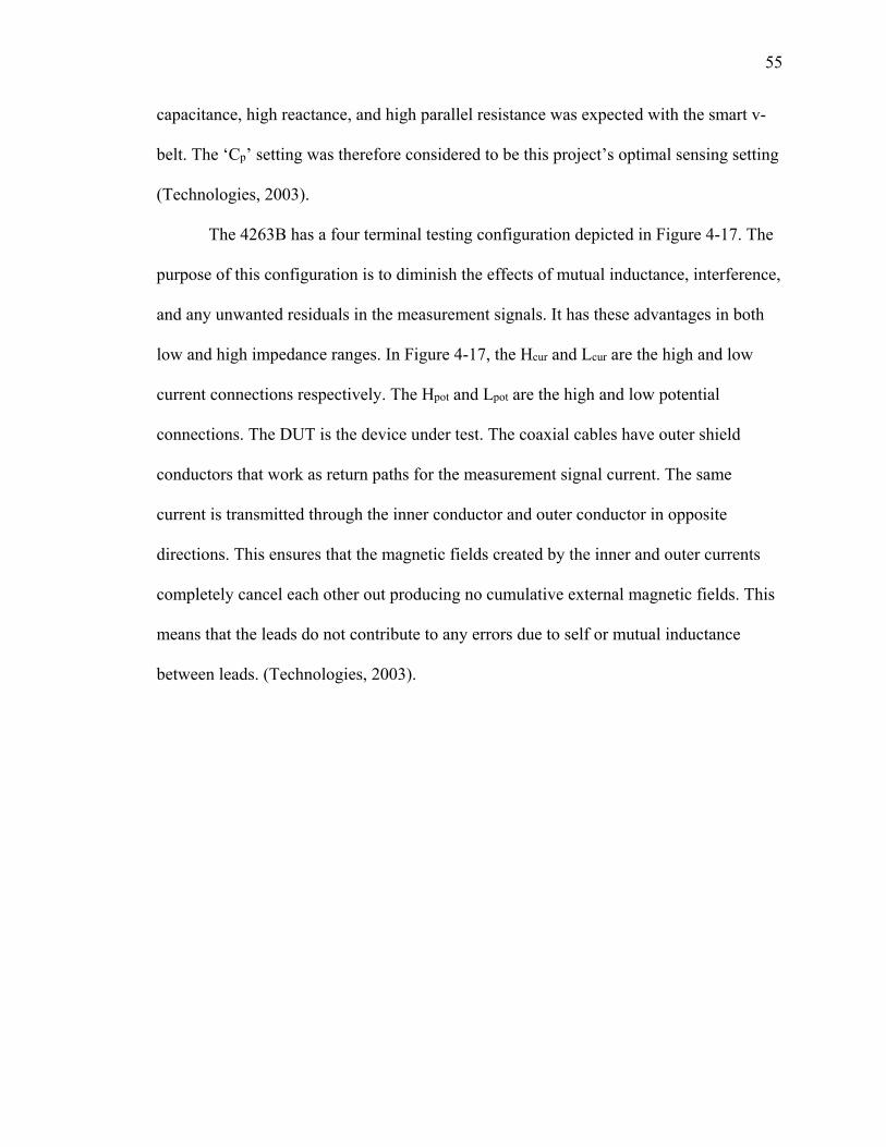
55
capacitance, high reactance, and high parallel resistance was expected with the smart v-
belt. The ‘Cp’ setting was therefore considered to be this project’s optimal sensing setting
(Technologies, 2003).
The 4263B has a four terminal testing configuration depicted in Figure 4-17. The
purpose of this configuration is to diminish the effects of mutual inductance, interference,
and any unwanted residuals in the measurement signals. It has these advantages in both
low and high impedance ranges. In Figure 4-17, the Hcur and Lcur are the high and low
current connections respectively. The Hpot and Lpot are the high and low potential
connections. The DUT is the device under test. The coaxial cables have outer shield
conductors that work as return paths for the measurement signal current. The same
current is transmitted through the inner conductor and outer conductor in opposite
directions. This ensures that the magnetic fields created by the inner and outer currents
completely cancel each other out producing no cumulative external magnetic fields. This
means that the leads do not contribute to any errors due to self or mutual inductance
between leads. (Technologies, 2003).
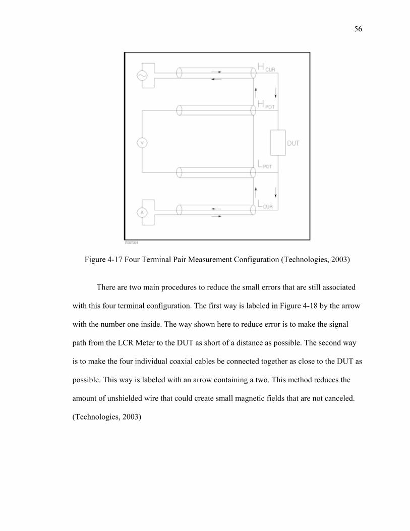
56
Figure 4-17 Four Terminal Pair Measurement Configuration (Technologies, 2003)
There are two main procedures to reduce the small errors that are still associated
with this four terminal configuration. The first way is labeled in Figure 4-18 by the arrow
with the number one inside. The way shown here to reduce error is to make the signal
path from the LCR Meter to the DUT as short of a distance as possible. The second way
is to make the four individual coaxial cables be connected together as close to the DUT as
possible. This way is labeled with an arrow containing a two. This method reduces the
amount of unshielded wire that could create small magnetic fields that are not canceled.
(Technologies, 2003)
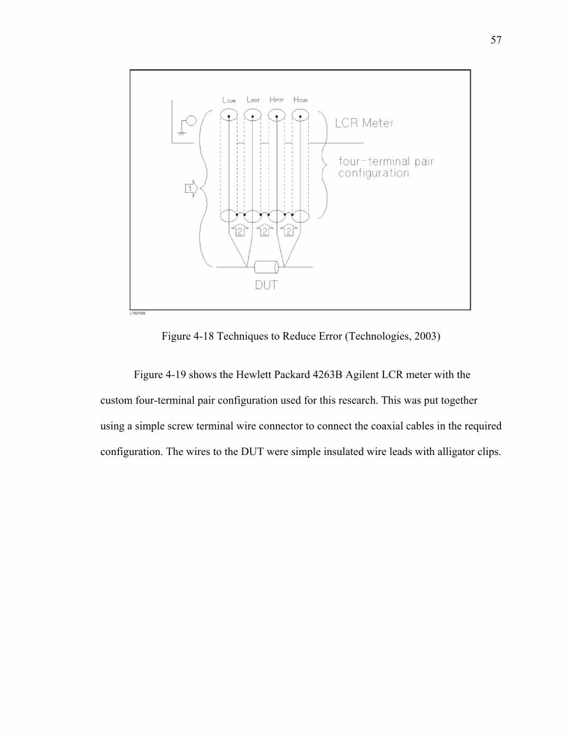
57
Figure 4-18 Techniques to Reduce Error (Technologies, 2003)
Figure 4-19 shows the Hewlett Packard 4263B Agilent LCR meter with the
custom four-terminal pair configuration used for this research. This was put together
using a simple screw terminal wire connector to connect the coaxial cables in the required
configuration. The wires to the DUT were simple insulated wire leads with alligator clips.
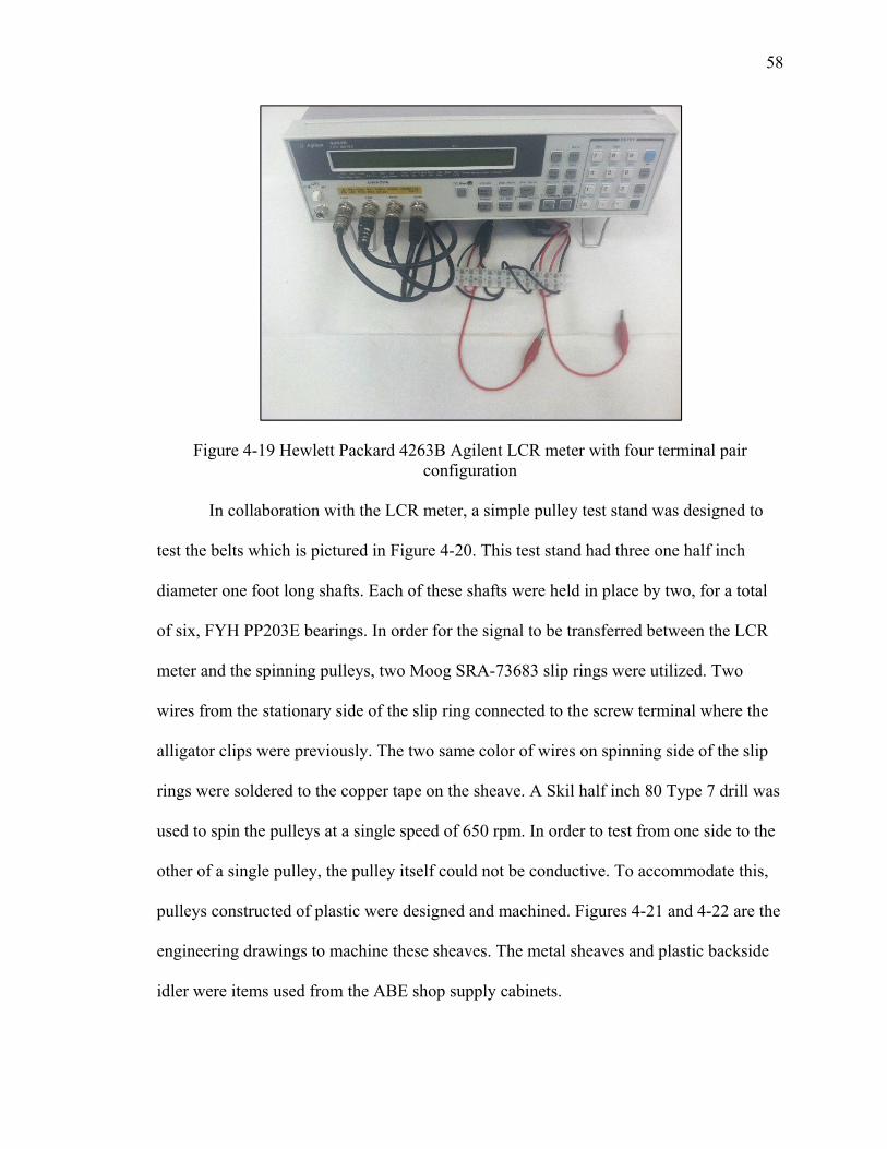
58
Figure 4-19 Hewlett Packard 4263B Agilent LCR meter with four terminal pair configuration
In collaboration with the LCR meter, a simple pulley test stand was designed to
test the belts which is pictured in Figure 4-20. This test stand had three one half inch
diameter one foot long shafts. Each of these shafts were held in place by two, for a total
of six, FYH PP203E bearings. In order for the signal to be transferred between the LCR
meter and the spinning pulleys, two Moog SRA-73683 slip rings were utilized. Two
wires from the stationary side of the slip ring connected to the screw terminal where the
alligator clips were previously. The two same color of wires on spinning side of the slip
rings were soldered to the copper tape on the sheave. A Skil half inch 80 Type 7 drill was
used to spin the pulleys at a single speed of 650 rpm. In order to test from one side to the
other of a single pulley, the pulley itself could not be conductive. To accommodate this,
pulleys constructed of plastic were designed and machined. Figures 4-21 and 4-22 are the
engineering drawings to machine these sheaves. The metal sheaves and plastic backside
idler were items used from the ABE shop supply cabinets.
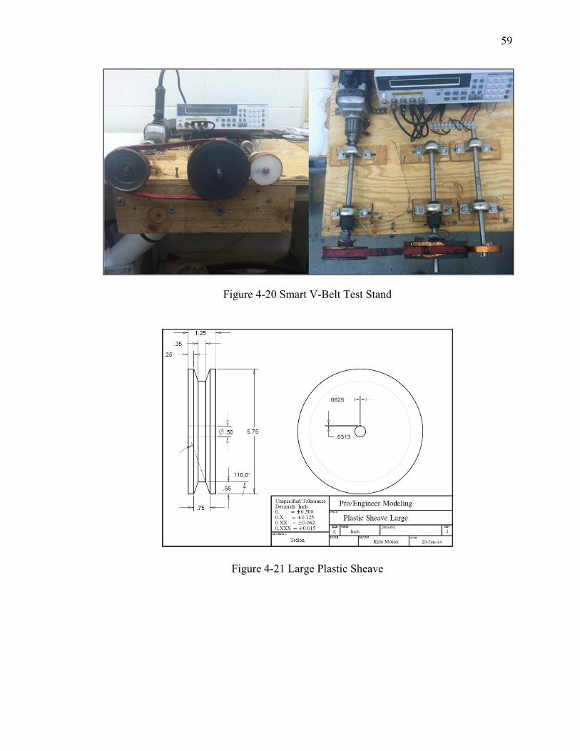
59
Figure 4-20 Smart V-Belt Test Stand
Figure 4-21 Large Plastic Sheave
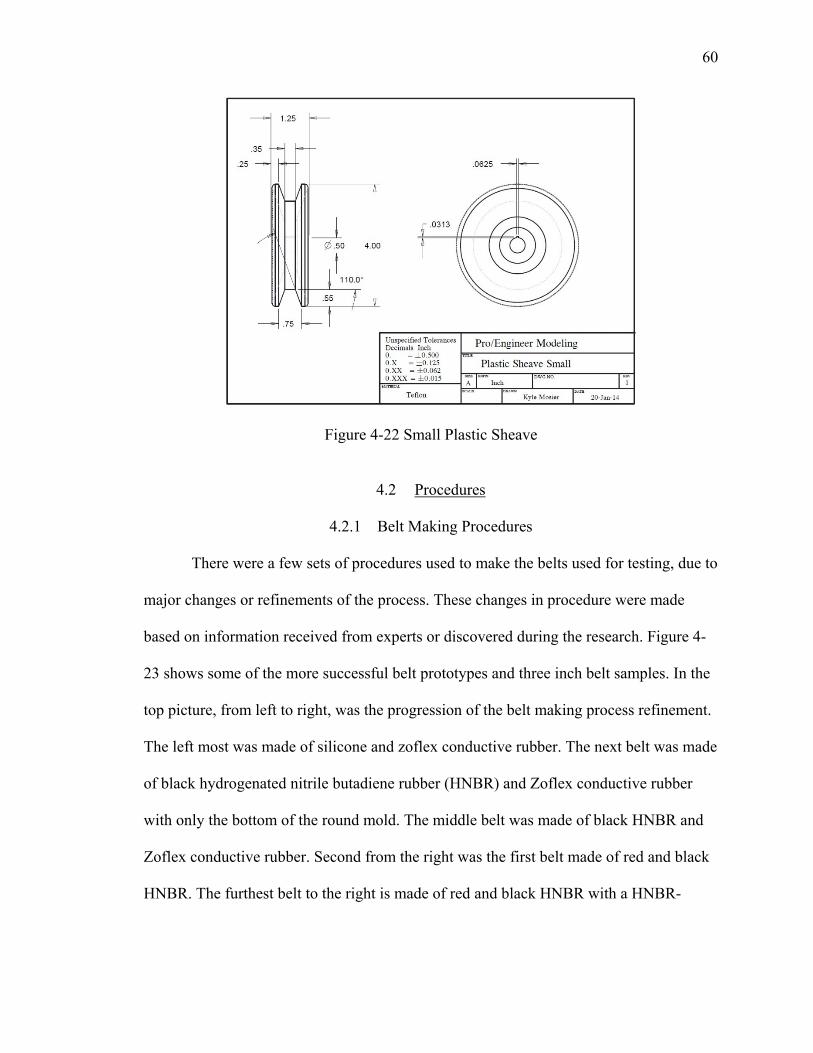
60
Figure 4-22 Small Plastic Sheave
4.2 Procedures
4.2.1 Belt Making Procedures
There were a few sets of procedures used to make the belts used for testing, due to
major changes or refinements of the process. These changes in procedure were made
based on information received from experts or discovered during the research. Figure 4-
23 shows some of the more successful belt prototypes and three inch belt samples. In the
top picture, from left to right, was the progression of the belt making process refinement.
The left most was made of silicone and zoflex conductive rubber. The next belt was made
of black hydrogenated nitrile butadiene rubber (HNBR) and Zoflex conductive rubber
with only the bottom of the round mold. The middle belt was made of black HNBR and
Zoflex conductive rubber. Second from the right was the first belt made of red and black
HNBR. The furthest belt to the right is made of red and black HNBR with a HNBR-
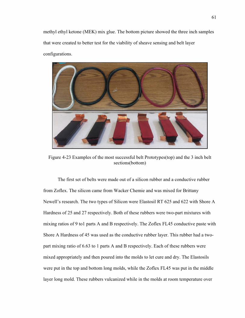
61
methyl ethyl ketone (MEK) mix glue. The bottom picture showed the three inch samples
that were created to better test for the viability of sheave sensing and belt layer
configurations.
Figure 4-23 Examples of the most successful belt Prototypes(top) and the 3 inch belt sections(bottom)
The first set of belts were made out of a silicon rubber and a conductive rubber
from Zoflex. The silicon came from Wacker Chemie and was mixed for Brittany
Newell’s research. The two types of Silicon were Elastosil RT 625 and 622 with Shore A
Hardness of 25 and 27 respectively. Both of these rubbers were two-part mixtures with
mixing ratios of 9 to1 parts A and B respectively. The Zoflex FL45 conductive paste with
Shore A Hardness of 45 was used as the conductive rubber layer. This rubber had a two-
part mixing ratio of 6.63 to 1 parts A and B respectively. Each of these rubbers were
mixed appropriately and then poured into the molds to let cure and dry. The Elastosils
were put in the top and bottom long molds, while the Zoflex FL45 was put in the middle
layer long mold. These rubbers vulcanized while in the molds at room temperature over
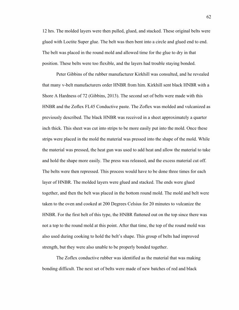
62
12 hrs. The molded layers were then pulled, glued, and stacked. These original belts were
glued with Loctite Super glue. The belt was then bent into a circle and glued end to end.
The belt was placed in the round mold and allowed time for the glue to dry in that
position. These belts were too flexible, and the layers had trouble staying bonded.
Peter Gibbins of the rubber manufacturer Kirkhill was consulted, and he revealed
that many v-belt manufacturers order HNBR from him. Kirkhill sent black HNBR with a
Shore A Hardness of 72 (Gibbins, 2013). The second set of belts were made with this
HNBR and the Zoflex FL45 Conductive paste. The Zoflex was molded and vulcanized as
previously described. The black HNBR was received in a sheet approximately a quarter
inch thick. This sheet was cut into strips to be more easily put into the mold. Once these
strips were placed in the mold the material was pressed into the shape of the mold. While
the material was pressed, the heat gun was used to add heat and allow the material to take
and hold the shape more easily. The press was released, and the excess material cut off.
The belts were then repressed. This process would have to be done three times for each
layer of HNBR. The molded layers were glued and stacked. The ends were glued
together, and then the belt was placed in the bottom round mold. The mold and belt were
taken to the oven and cooked at 200 Degrees Celsius for 20 minutes to vulcanize the
HNBR. For the first belt of this type, the HNBR flattened out on the top since there was
not a top to the round mold at this point. After that time, the top of the round mold was
also used during cooking to hold the belt’s shape. This group of belts had improved
strength, but they were also unable to be properly bonded together.
The Zoflex conductive rubber was identified as the material that was making
bonding difficult. The next set of belts were made of new batches of red and black
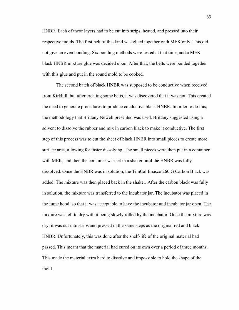
63
HNBR. Each of these layers had to be cut into strips, heated, and pressed into their
respective molds. The first belt of this kind was glued together with MEK only. This did
not give an even bonding. Six bonding methods were tested at that time, and a MEK-
black HNBR mixture glue was decided upon. After that, the belts were bonded together
with this glue and put in the round mold to be cooked.
The second batch of black HNBR was supposed to be conductive when received
from Kirkhill, but after creating some belts, it was discovered that it was not. This created
the need to generate procedures to produce conductive black HNBR. In order to do this,
the methodology that Brittany Newell presented was used. Brittany suggested using a
solvent to dissolve the rubber and mix in carbon black to make it conductive. The first
step of this process was to cut the sheet of black HNBR into small pieces to create more
surface area, allowing for faster dissolving. The small pieces were then put in a container
with MEK, and then the container was set in a shaker until the HNBR was fully
dissolved. Once the HNBR was in solution, the TimCal Enasco 260 G Carbon Black was
added. The mixture was then placed back in the shaker. After the carbon black was fully
in solution, the mixture was transferred to the incubator jar. The incubator was placed in
the fume hood, so that it was acceptable to have the incubator and incubator jar open. The
mixture was left to dry with it being slowly rolled by the incubator. Once the mixture was
dry, it was cut into strips and pressed in the same steps as the original red and black
HNBR. Unfortunately, this was done after the shelf-life of the original material had
passed. This meant that the material had cured on its own over a period of three months.
This made the material extra hard to dissolve and impossible to hold the shape of the
mold.
64
The optimal configuration of the layers in the belts and the optimal configuration
of the sheave sensing were identified as areas that needed further research. For this
investigation, there were six-three inch belt section samples created. In order to get the
needed sections of each type of HNBR in one pressing cycle, half of each mold was filled
with each kind of material. The end result of these pressings was pictured in Figure 4-24.
The red and black HNBR material, from each mold was cut into three inch sections. The
sections of each type were glued together with the HNBR glue to create the samples
pictured in Figure 4-23.
Figure 4-24 Pressed black and red HNBR for three inch sections
4.2.2 Belt Testing Procedures
The first set of preliminary tests were run on existing examples of belts. A v-belt
donated by Carlisle Transportation Products was taken apart, so that the different
materials used in its construction could be tested for capacitance and resistance using the
LCR meter. The material sections that were tested were pictured in Figure 4-25.
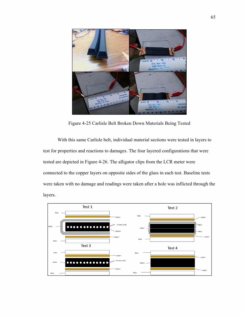
65
Figure 4-25 Carlisle Belt Broken Down Materials Being Tested
With this same Carlisle belt, individual material sections were tested in layers to
test for properties and reactions to damages. The four layered configurations that were
tested are depicted in Figure 4-26. The alligator clips from the LCR meter were
connected to the copper layers on opposite sides of the glass in each test. Baseline tests
were taken with no damage and readings were taken after a hole was inflicted through the
layers.

66
Figure 4-26 Flat Plate Tests of current belt sections
The same Carlisle belt tests were run to see the reading changes according to
weight hung from the belt. This was to simulate being able to read the tension on the belt
in a pulley system. The apparatus pictured in Figure 4-27 was constructed and utilized to
run this weight test. The belt had two holes drilled into it at each end and a threaded rod
stuck through them. Nuts and washers were added to clamp the belt and hold the threaded
rod in the belt. One of these rods was put into two holes that were drilled into two 2 by
4s. These 2 by 4s were clamped to the table. A slotted weight hanging rod was hung by
chain from the other threaded rod. Copper tape was added to the top and bottom of the
belt to take resistance and capacitance readings using the LCR meter. Ten pound slotted
weights were added to the apparatus, and measurements were taken from just the weight
of the chain, up to 100 pounds.
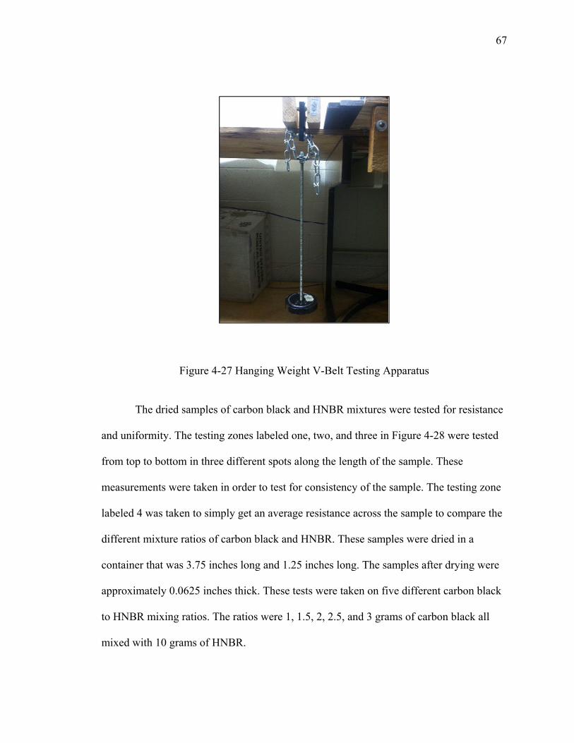
67
Figure 4-27 Hanging Weight V-Belt Testing Apparatus
The dried samples of carbon black and HNBR mixtures were tested for resistance
and uniformity. The testing zones labeled one, two, and three in Figure 4-28 were tested
from top to bottom in three different spots along the length of the sample. These
measurements were taken in order to test for consistency of the sample. The testing zone
labeled 4 was taken to simply get an average resistance across the sample to compare the
different mixture ratios of carbon black and HNBR. These samples were dried in a
container that was 3.75 inches long and 1.25 inches long. The samples after drying were
approximately 0.0625 inches thick. These tests were taken on five different carbon black
to HNBR mixing ratios. The ratios were 1, 1.5, 2, 2.5, and 3 grams of carbon black all
mixed with 10 grams of HNBR.
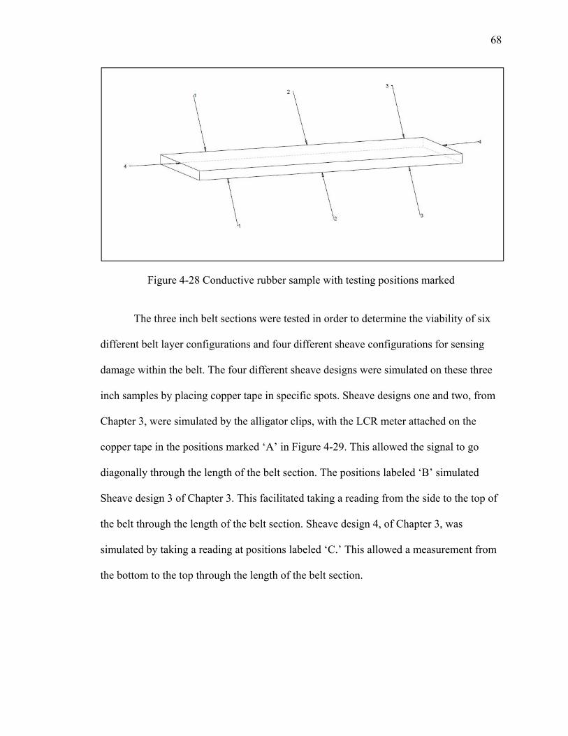
68
Figure 4-28 Conductive rubber sample with testing positions marked
The three inch belt sections were tested in order to determine the viability of six
different belt layer configurations and four different sheave configurations for sensing
damage within the belt. The four different sheave designs were simulated on these three
inch samples by placing copper tape in specific spots. Sheave designs one and two, from
Chapter 3, were simulated by the alligator clips, with the LCR meter attached on the
copper tape in the positions marked ‘A’ in Figure 4-29. This allowed the signal to go
diagonally through the length of the belt section. The positions labeled ‘B’ simulated
Sheave design 3 of Chapter 3. This facilitated taking a reading from the side to the top of
the belt through the length of the belt section. Sheave design 4, of Chapter 3, was
simulated by taking a reading at positions labeled ‘C.’ This allowed a measurement from
the bottom to the top through the length of the belt section.
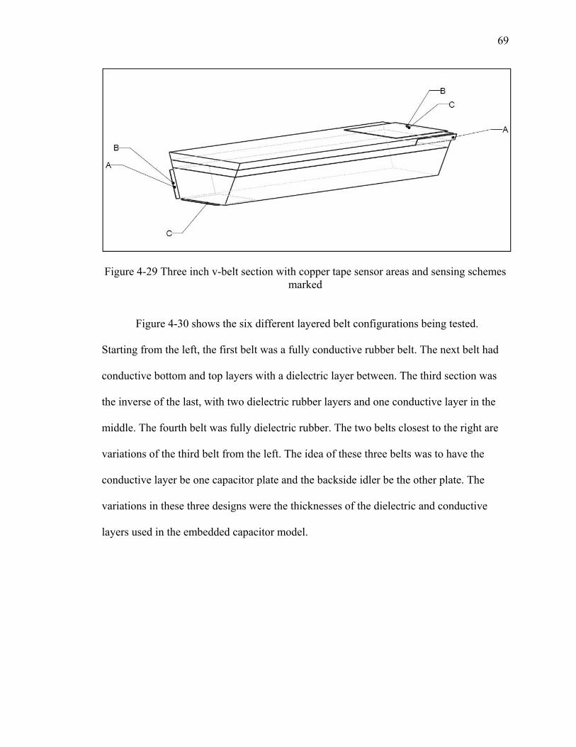
69
Figure 4-29 Three inch v-belt section with copper tape sensor areas and sensing schemes marked
Figure 4-30 shows the six different layered belt configurations being tested.
Starting from the left, the first belt was a fully conductive rubber belt. The next belt had
conductive bottom and top layers with a dielectric layer between. The third section was
the inverse of the last, with two dielectric rubber layers and one conductive layer in the
middle. The fourth belt was fully dielectric rubber. The two belts closest to the right are
variations of the third belt from the left. The idea of these three belts was to have the
conductive layer be one capacitor plate and the backside idler be the other plate. The
variations in these three designs were the thicknesses of the dielectric and conductive
layers used in the embedded capacitor model.
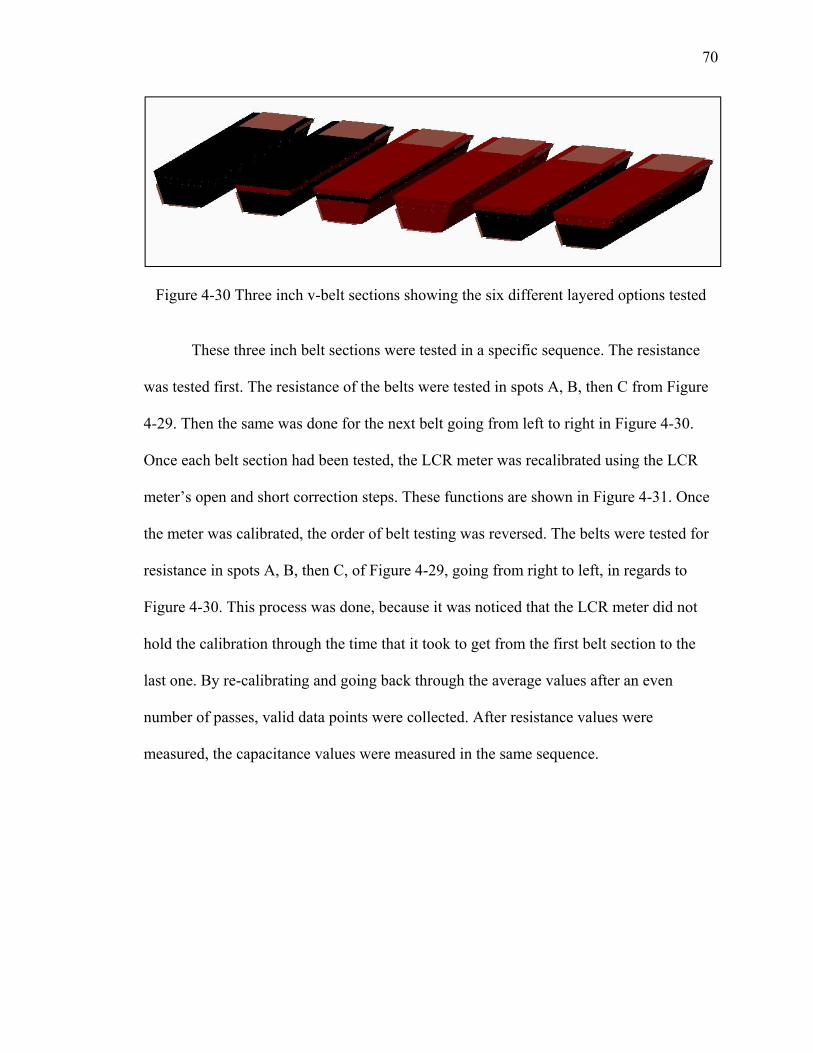
70
Figure 4-30 Three inch v-belt sections showing the six different layered options tested
These three inch belt sections were tested in a specific sequence. The resistance
was tested first. The resistance of the belts were tested in spots A, B, then C from Figure
4-29. Then the same was done for the next belt going from left to right in Figure 4-30.
Once each belt section had been tested, the LCR meter was recalibrated using the LCR
meter’s open and short correction steps. These functions are shown in Figure 4-31. Once
the meter was calibrated, the order of belt testing was reversed. The belts were tested for
resistance in spots A, B, then C, of Figure 4-29, going from right to left, in regards to
Figure 4-30. This process was done, because it was noticed that the LCR meter did not
hold the calibration through the time that it took to get from the first belt section to the
last one. By re-calibrating and going back through the average values after an even
number of passes, valid data points were collected. After resistance values were
measured, the capacitance values were measured in the same sequence.

71
Figure 4-31 Pictures of testing(left), short correction(top), and open correction(bottom) being conducted
Measurements were taken in the previously described fashion before damage,
after layer separation, after a hole being made, and after an abrasion was inflicted. These
damages were cumulative. Figure 4-32 shows the damages being inflicted in the order,
left to right, that they were performed.
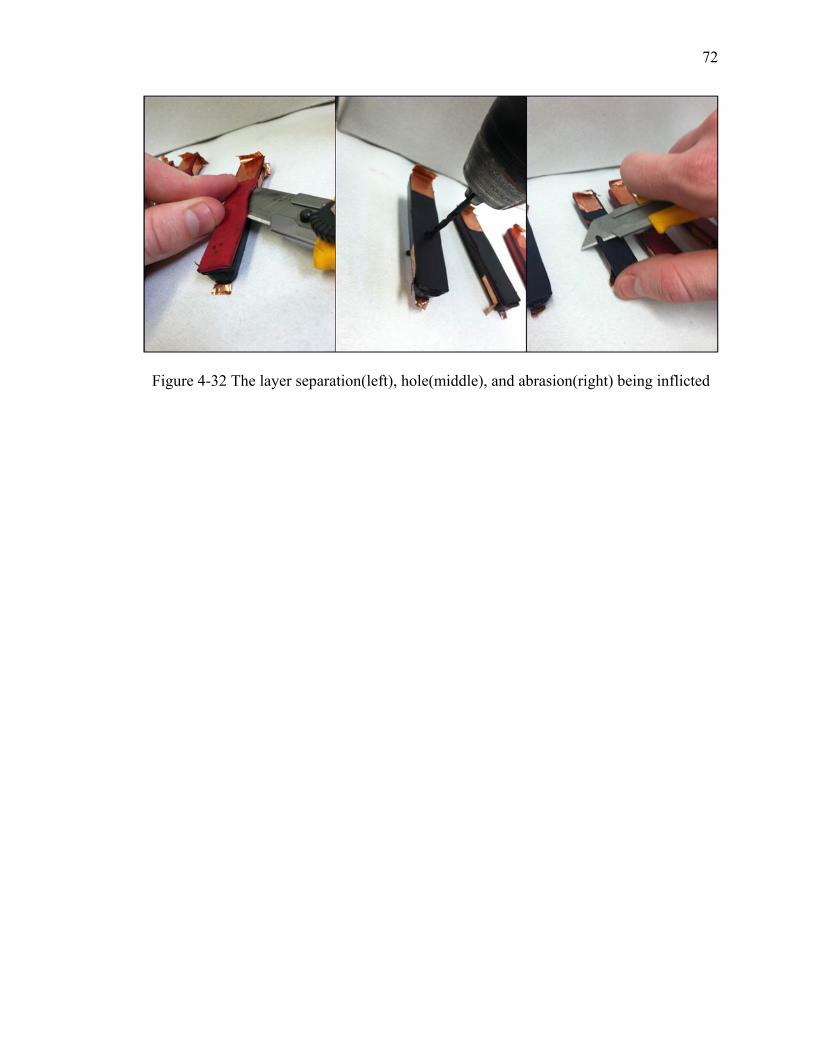
72
Figure 4-32 The layer separation(left), hole(middle), and abrasion(right) being inflicted
73
CHAPTER 5. TEST RESULTS
5.1 Carlisle Belt Material Tests
The preliminary research started with taking these readings with the current
materials used in an example belt. These results are from a Carlisle v-belt. Figure 5-1 is a
pictorial representation of the data gathered on the materials found in this belt. This
figure shows each of the material sections that were tested and their major measurement
values. A picture of the original belt is also shown in the bottom left of the figure. An
interesting discovery was that the aramid tension cord had the lowest resistance. It was
anticipated that the fabric would have the highest resistance, but the rubber body resulted
in the highest resistance. All of these readings seemed to have large standard deviations
with the fabric layer having the highest relative to the average at 8.83kΩ. This standard
deviation was a slightly over a third of the average value, meaning the coefficient of
variation is 0.338. None of the other data had this much variability.
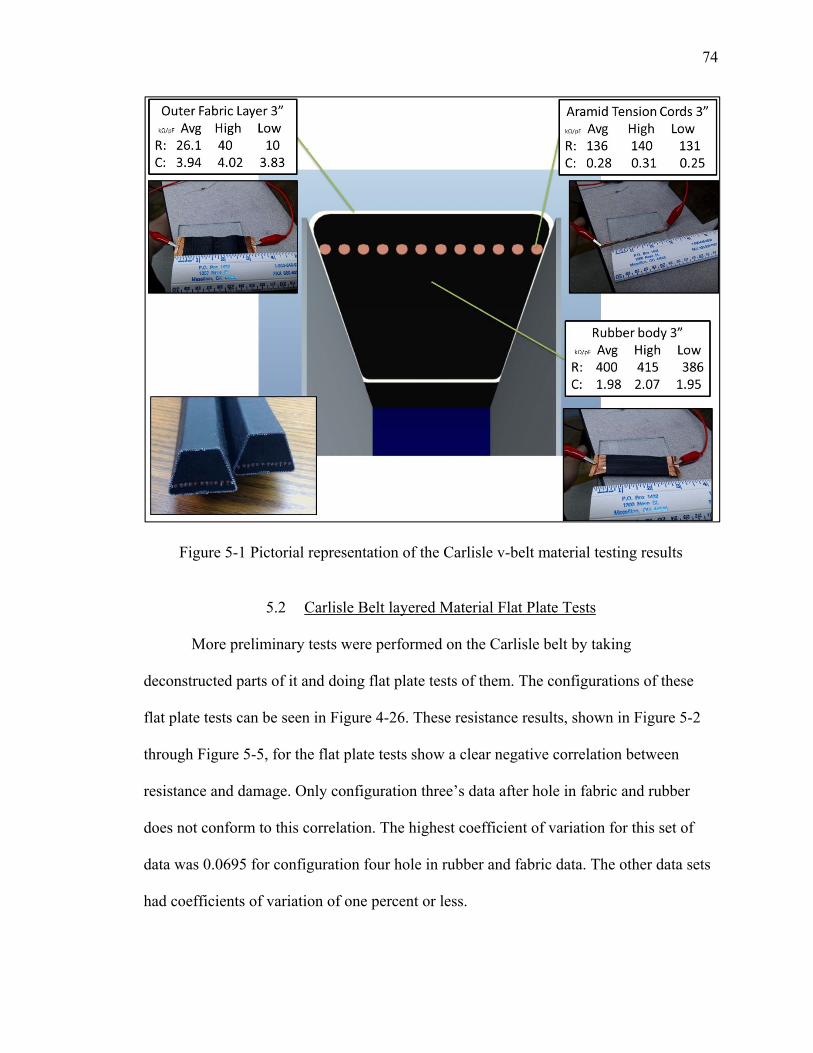
74
Figure 5-1 Pictorial representation of the Carlisle v-belt material testing results
5.2 Carlisle Belt layered Material Flat Plate Tests
More preliminary tests were performed on the Carlisle belt by taking
deconstructed parts of it and doing flat plate tests of them. The configurations of these
flat plate tests can be seen in Figure 4-26. These resistance results, shown in Figure 5-2
through Figure 5-5, for the flat plate tests show a clear negative correlation between
resistance and damage. Only configuration three’s data after hole in fabric and rubber
does not conform to this correlation. The highest coefficient of variation for this set of
data was 0.0695 for configuration four hole in rubber and fabric data. The other data sets
had coefficients of variation of one percent or less.

75
Figure 5-2 Resistance readings of flat plate test 1 vs damage with 95% CI
Figure 5-3 Resistance readings of flat plate test 2 vs damage with 95% CI
50 kΩ
51 kΩ
52 kΩ
53 kΩ
54 kΩ
55 kΩ
56 kΩ
57 kΩ
58 kΩ
59 kΩ
60 kΩ
Set 1 Set 1, hole in rubber Set 1, hole in rubber and fabric
Resistance averages of Set 1 tests
46 kΩ
48 kΩ
50 kΩ
52 kΩ
54 kΩ
56 kΩ
58 kΩ
Set 2 Set 2, hole
Resistance averages of Set 2 tests
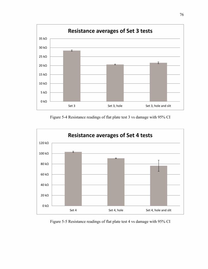
76
Figure 5-4 Resistance readings of flat plate test 3 vs damage with 95% CI
Figure 5-5 Resistance readings of flat plate test 4 vs damage with 95% CI
0 kΩ
5 kΩ
10 kΩ
15 kΩ
20 kΩ
25 kΩ
30 kΩ
35 kΩ
Set 3 Set 3, hole Set 3, hole and slit
Resistance averages of Set 3 tests
0 kΩ
20 kΩ
40 kΩ
60 kΩ
80 kΩ
100 kΩ
120 kΩ
Set 4 Set 4, hole Set 4, hole and slit
Resistance averages of Set 4 tests
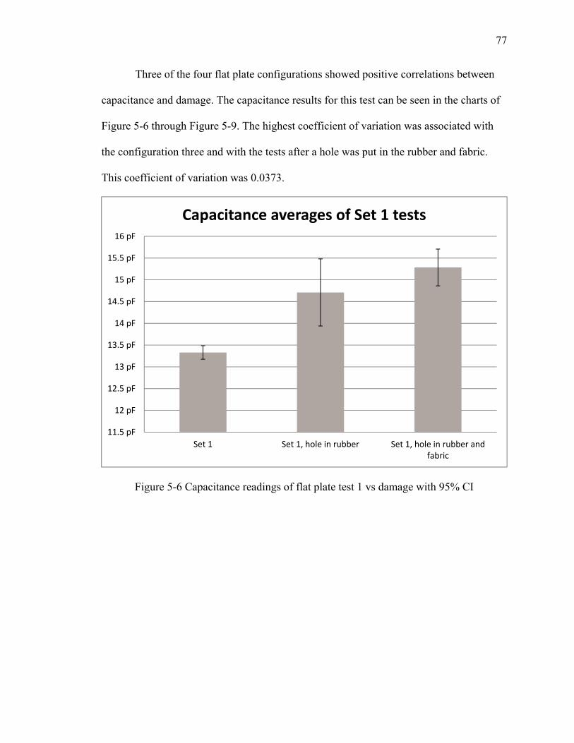
77
Three of the four flat plate configurations showed positive correlations between
capacitance and damage. The capacitance results for this test can be seen in the charts of
Figure 5-6 through Figure 5-9. The highest coefficient of variation was associated with
the configuration three and with the tests after a hole was put in the rubber and fabric.
This coefficient of variation was 0.0373.
Figure 5-6 Capacitance readings of flat plate test 1 vs damage with 95% CI
11.5 pF
12 pF
12.5 pF
13 pF
13.5 pF
14 pF
14.5 pF
15 pF
15.5 pF
16 pF
Set 1 Set 1, hole in rubber Set 1, hole in rubber andfabric
Capacitance averages of Set 1 tests
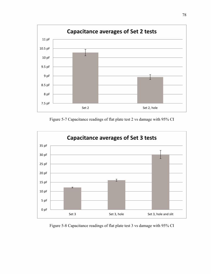
78
Figure 5-7 Capacitance readings of flat plate test 2 vs damage with 95% CI
Figure 5-8 Capacitance readings of flat plate test 3 vs damage with 95% CI
7.5 pF
8 pF
8.5 pF
9 pF
9.5 pF
10 pF
10.5 pF
11 pF
Set 2 Set 2, hole
Capacitance averages of Set 2 tests
0 pF
5 pF
10 pF
15 pF
20 pF
25 pF
30 pF
35 pF
Set 3 Set 3, hole Set 3, hole and slit
Capacitance averages of Set 3 tests
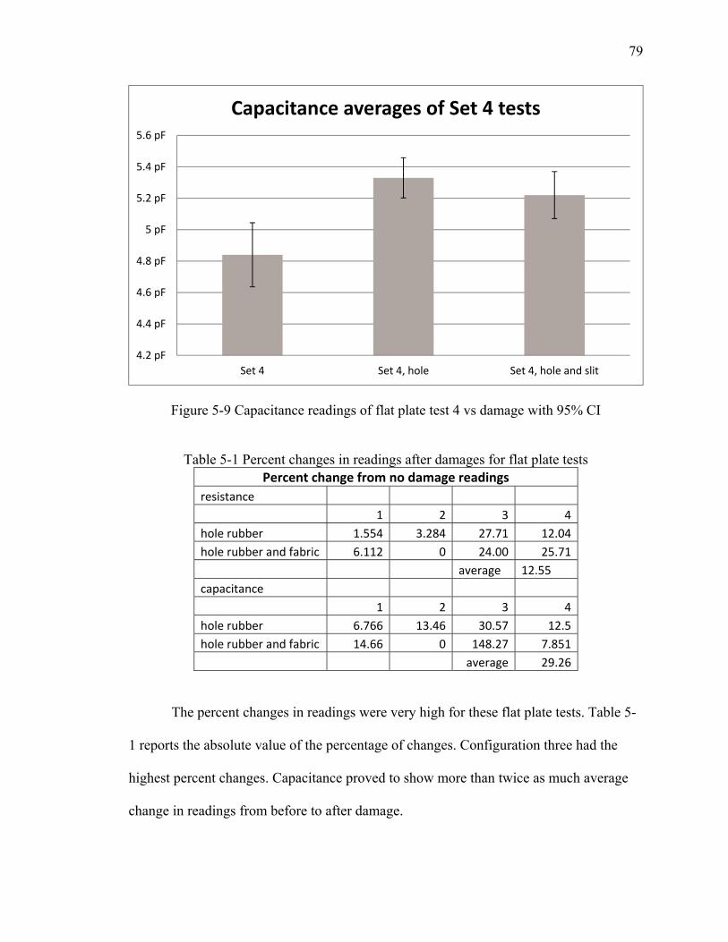
79
Figure 5-9 Capacitance readings of flat plate test 4 vs damage with 95% CI
Table 5-1 Percent changes in readings after damages for flat plate tests Percent change from no damage readings
resistance
1 2 3 4
hole rubber 1.554 3.284 27.71 12.04
hole rubber and fabric 6.112 0 24.00 25.71
average 12.55
capacitance
1 2 3 4
hole rubber 6.766 13.46 30.57 12.5
hole rubber and fabric 14.66 0 148.27 7.851
average 29.26
The percent changes in readings were very high for these flat plate tests. Table 5-
1 reports the absolute value of the percentage of changes. Configuration three had the
highest percent changes. Capacitance proved to show more than twice as much average
change in readings from before to after damage.
4.2 pF
4.4 pF
4.6 pF
4.8 pF
5 pF
5.2 pF
5.4 pF
5.6 pF
Set 4 Set 4, hole Set 4, hole and slit
Capacitance averages of Set 4 tests
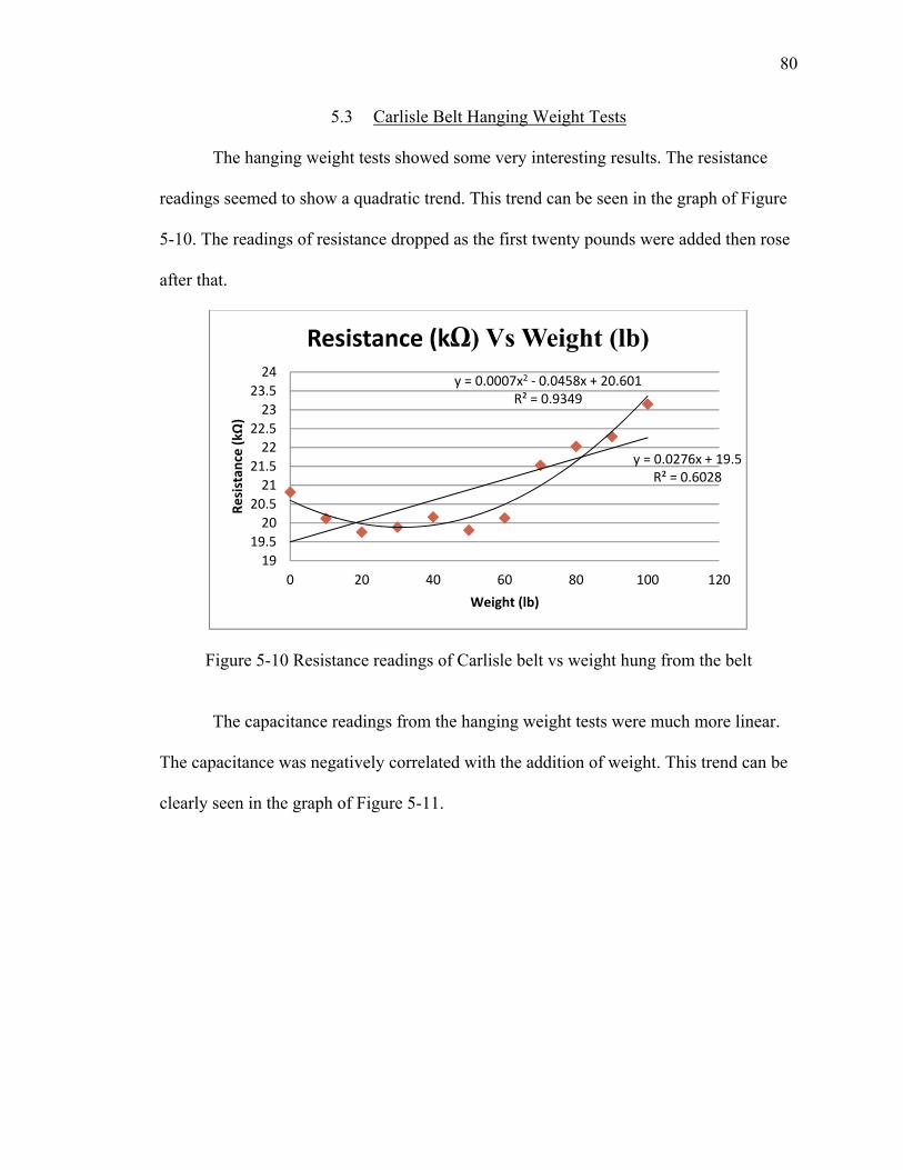
80
5.3 Carlisle Belt Hanging Weight Tests
The hanging weight tests showed some very interesting results. The resistance
readings seemed to show a quadratic trend. This trend can be seen in the graph of Figure
5-10. The readings of resistance dropped as the first twenty pounds were added then rose
after that.
Figure 5-10 Resistance readings of Carlisle belt vs weight hung from the belt
The capacitance readings from the hanging weight tests were much more linear.
The capacitance was negatively correlated with the addition of weight. This trend can be
clearly seen in the graph of Figure 5-11.
y = 0.0007x2 ‐ 0.0458x + 20.601R² = 0.9349
y = 0.0276x + 19.5R² = 0.6028
19
19.5
20
20.5
21
21.5
22
22.5
23
23.5
24
0 20 40 60 80 100 120
Resistan
ce (kΩ
)
Weight (lb)
Resistance (kΩ) Vs Weight (lb)
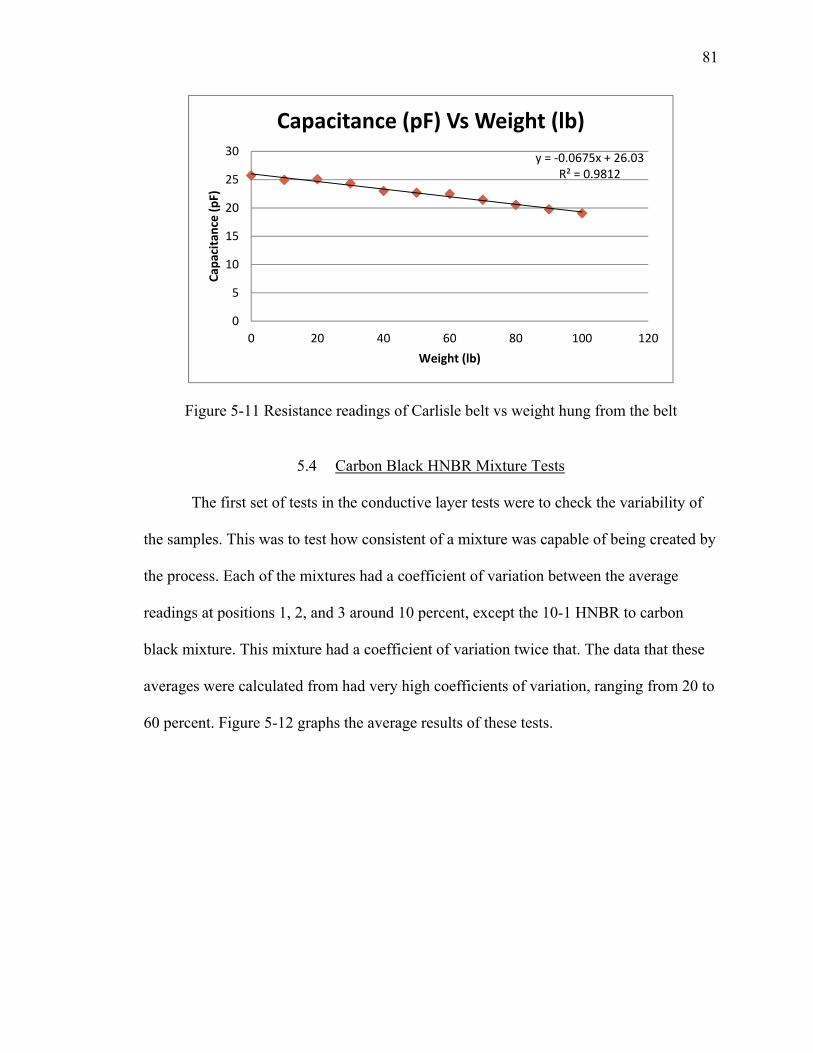
81
Figure 5-11 Resistance readings of Carlisle belt vs weight hung from the belt
5.4 Carbon Black HNBR Mixture Tests
The first set of tests in the conductive layer tests were to check the variability of
the samples. This was to test how consistent of a mixture was capable of being created by
the process. Each of the mixtures had a coefficient of variation between the average
readings at positions 1, 2, and 3 around 10 percent, except the 10-1 HNBR to carbon
black mixture. This mixture had a coefficient of variation twice that. The data that these
averages were calculated from had very high coefficients of variation, ranging from 20 to
60 percent. Figure 5-12 graphs the average results of these tests.
y = ‐0.0675x + 26.03R² = 0.9812
0
5
10
15
20
25
30
0 20 40 60 80 100 120
Cap
acitan
ce (pF)
Weight (lb)
Capacitance (pF) Vs Weight (lb)
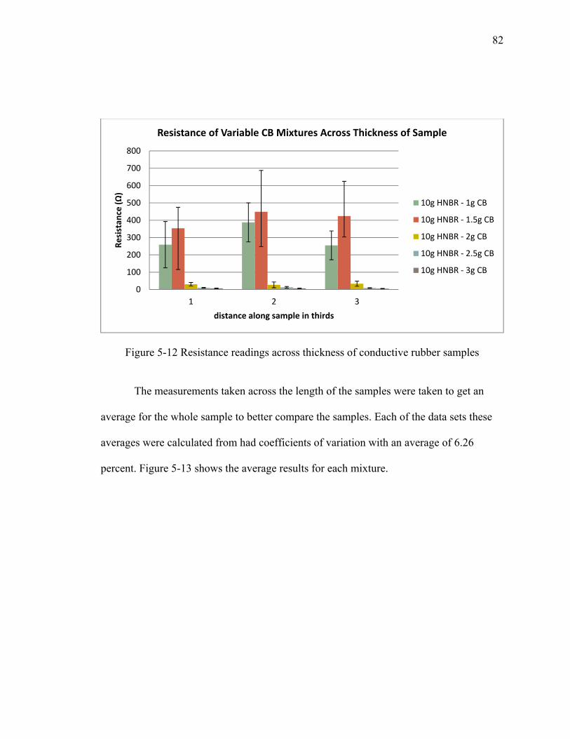
82
Figure 5-12 Resistance readings across thickness of conductive rubber samples
The measurements taken across the length of the samples were taken to get an
average for the whole sample to better compare the samples. Each of the data sets these
averages were calculated from had coefficients of variation with an average of 6.26
percent. Figure 5-13 shows the average results for each mixture.
0
100
200
300
400
500
600
700
800
1 2 3
Resistan
ce (Ω)
distance along sample in thirds
Resistance of Variable CB Mixtures Across Thickness of Sample
10g HNBR ‐ 1g CB
10g HNBR ‐ 1.5g CB
10g HNBR ‐ 2g CB
10g HNBR ‐ 2.5g CB
10g HNBR ‐ 3g CB
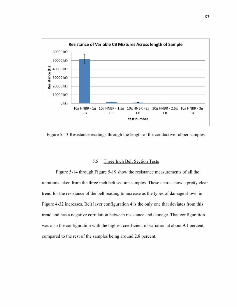
83
Figure 5-13 Resistance readings through the length of the conductive rubber samples
5.5 Three Inch Belt Section Tests
Figure 5-14 through Figure 5-19 show the resistance measurements of all the
iterations taken from the three inch belt section samples. These charts show a pretty clear
trend for the resistance of the belt reading to increase as the types of damage shown in
Figure 4-32 increases. Belt layer configuration 4 is the only one that deviates from this
trend and has a negative correlation between resistance and damage. That configuration
was also the configuration with the highest coefficient of variation at about 9.1 percent,
compared to the rest of the samples being around 2.8 percent.
0 kΩ
10000 kΩ
20000 kΩ
30000 kΩ
40000 kΩ
50000 kΩ
60000 kΩ
10g HNBR ‐ 1gCB
10g HNBR ‐ 1.5gCB
10g HNBR ‐ 2gCB
10g HNBR ‐ 2.5gCB
10g HNBR ‐ 3gCB
Resistan
ce (Ω)
test number
Resistance of Variable CB Mixtures Across length of Sample
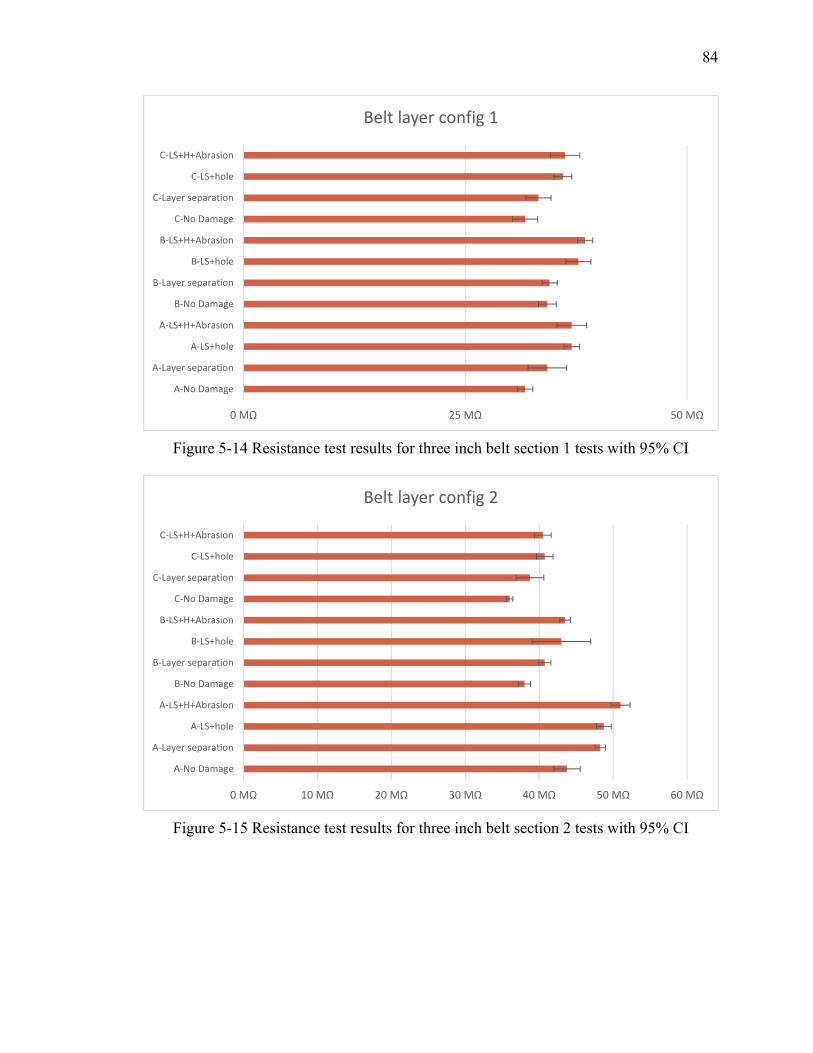
84
Figure 5-14 Resistance test results for three inch belt section 1 tests with 95% CI
Figure 5-15 Resistance test results for three inch belt section 2 tests with 95% CI
0 MΩ 25 MΩ 50 MΩ
A‐No Damage
A‐Layer separation
A‐LS+hole
A‐LS+H+Abrasion
B‐No Damage
B‐Layer separation
B‐LS+hole
B‐LS+H+Abrasion
C‐No Damage
C‐Layer separation
C‐LS+hole
C‐LS+H+Abrasion
Belt layer config 1
0 MΩ 10 MΩ 20 MΩ 30 MΩ 40 MΩ 50 MΩ 60 MΩ
A‐No Damage
A‐Layer separation
A‐LS+hole
A‐LS+H+Abrasion
B‐No Damage
B‐Layer separation
B‐LS+hole
B‐LS+H+Abrasion
C‐No Damage
C‐Layer separation
C‐LS+hole
C‐LS+H+Abrasion
Belt layer config 2
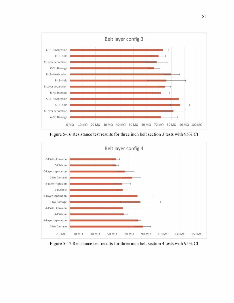
85
Figure 5-16 Resistance test results for three inch belt section 3 tests with 95% CI
Figure 5-17 Resistance test results for three inch belt section 4 tests with 95% CI
0 MΩ 10 MΩ 20 MΩ 30 MΩ 40 MΩ 50 MΩ 60 MΩ 70 MΩ 80 MΩ 90 MΩ 100 MΩ
A‐No Damage
A‐Layer separation
A‐LS+hole
A‐LS+H+Abrasion
B‐No Damage
B‐Layer separation
B‐LS+hole
B‐LS+H+Abrasion
C‐No Damage
C‐Layer separation
C‐LS+hole
C‐LS+H+Abrasion
Belt layer config 3
‐10 MΩ 10 MΩ 30 MΩ 50 MΩ 70 MΩ 90 MΩ 110 MΩ 130 MΩ 150 MΩ
A‐No Damage
A‐Layer separation
A‐LS+hole
A‐LS+H+Abrasion
B‐No Damage
B‐Layer separation
B‐LS+hole
B‐LS+H+Abrasion
C‐No Damage
C‐Layer separation
C‐LS+hole
C‐LS+H+Abrasion
Belt layer config 4
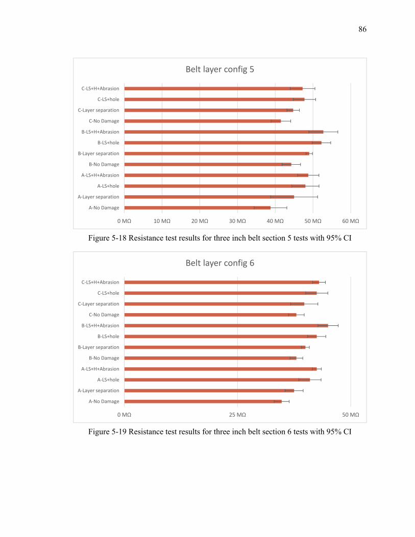
86
Figure 5-18 Resistance test results for three inch belt section 5 tests with 95% CI
Figure 5-19 Resistance test results for three inch belt section 6 tests with 95% CI
0 MΩ 10 MΩ 20 MΩ 30 MΩ 40 MΩ 50 MΩ 60 MΩ
A‐No Damage
A‐Layer separation
A‐LS+hole
A‐LS+H+Abrasion
B‐No Damage
B‐Layer separation
B‐LS+hole
B‐LS+H+Abrasion
C‐No Damage
C‐Layer separation
C‐LS+hole
C‐LS+H+Abrasion
Belt layer config 5
0 MΩ 25 MΩ 50 MΩ
A‐No Damage
A‐Layer separation
A‐LS+hole
A‐LS+H+Abrasion
B‐No Damage
B‐Layer separation
B‐LS+hole
B‐LS+H+Abrasion
C‐No Damage
C‐Layer separation
C‐LS+hole
C‐LS+H+Abrasion
Belt layer config 6
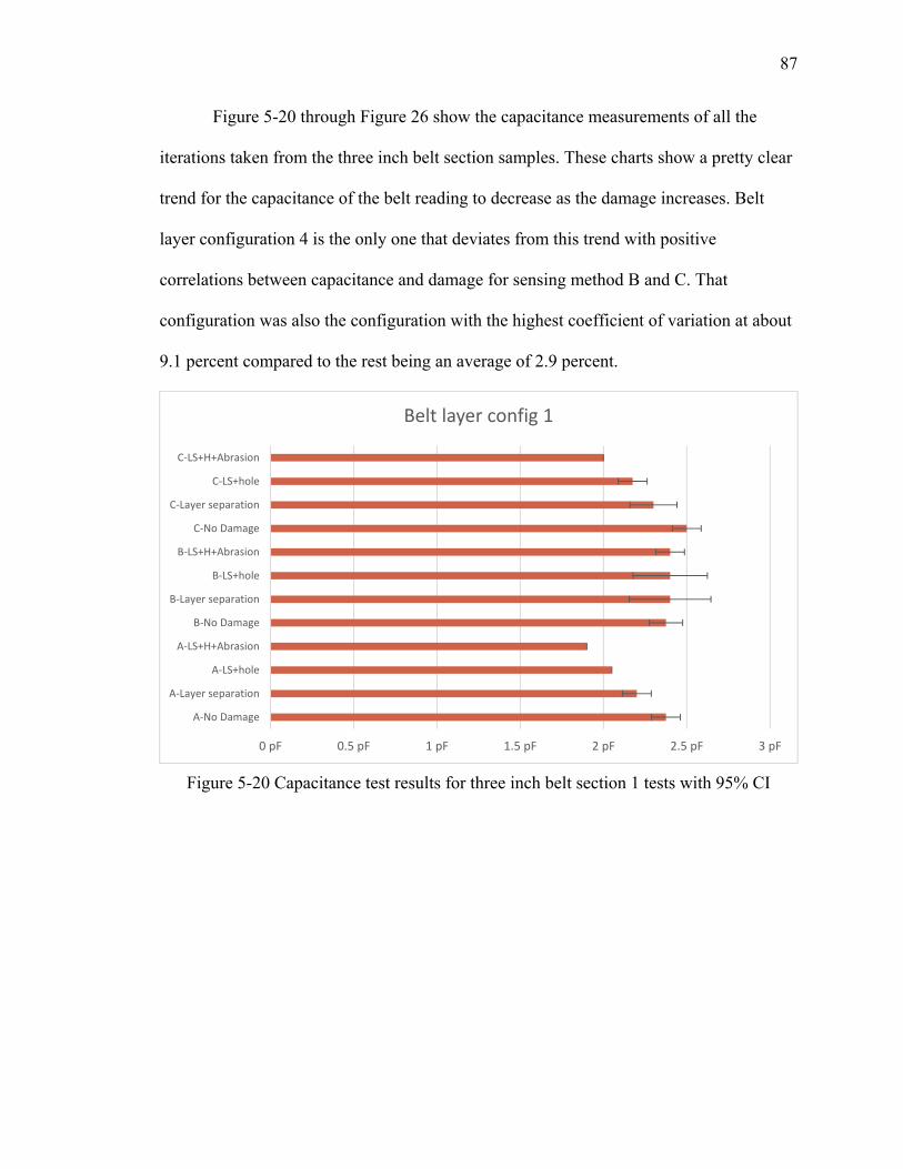
87
Figure 5-20 through Figure 26 show the capacitance measurements of all the
iterations taken from the three inch belt section samples. These charts show a pretty clear
trend for the capacitance of the belt reading to decrease as the damage increases. Belt
layer configuration 4 is the only one that deviates from this trend with positive
correlations between capacitance and damage for sensing method B and C. That
configuration was also the configuration with the highest coefficient of variation at about
9.1 percent compared to the rest being an average of 2.9 percent.
Figure 5-20 Capacitance test results for three inch belt section 1 tests with 95% CI
0 pF 0.5 pF 1 pF 1.5 pF 2 pF 2.5 pF 3 pF
A‐No Damage
A‐Layer separation
A‐LS+hole
A‐LS+H+Abrasion
B‐No Damage
B‐Layer separation
B‐LS+hole
B‐LS+H+Abrasion
C‐No Damage
C‐Layer separation
C‐LS+hole
C‐LS+H+Abrasion
Belt layer config 1
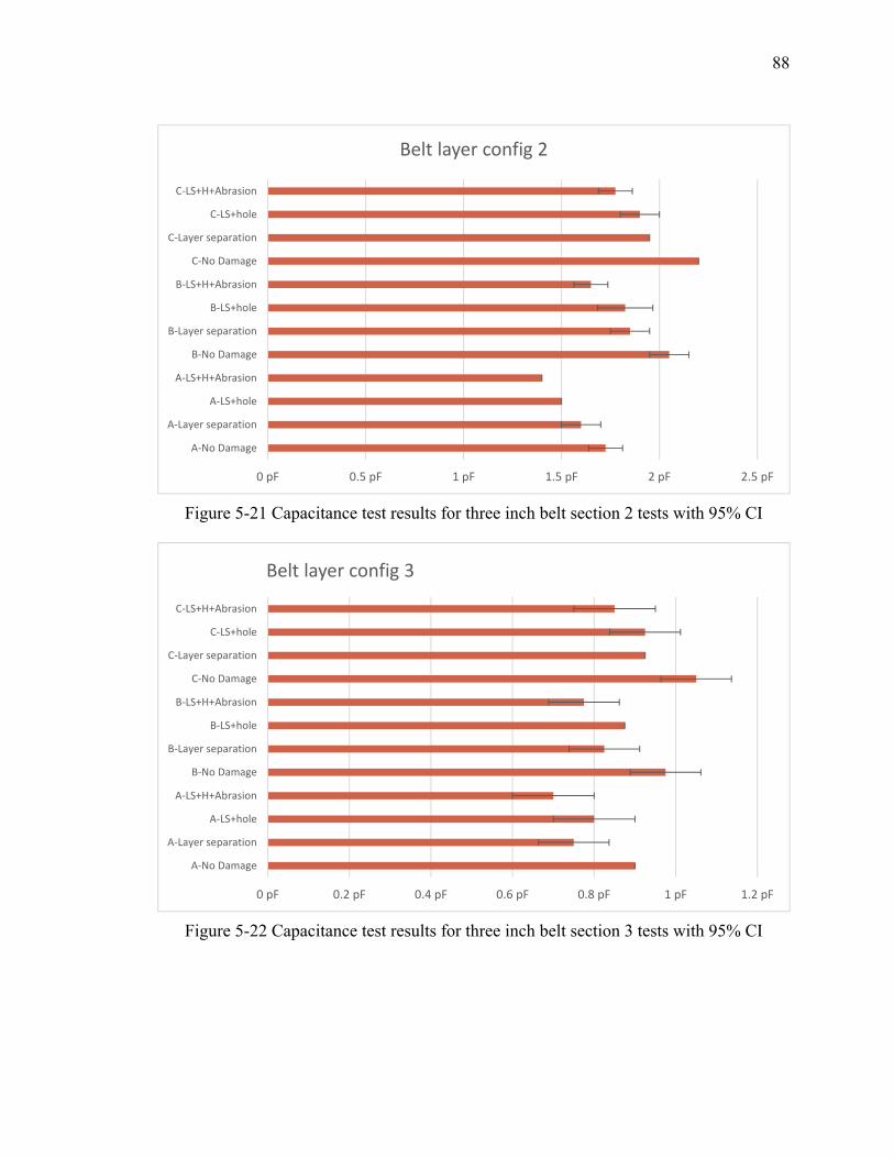
88
Figure 5-21 Capacitance test results for three inch belt section 2 tests with 95% CI
Figure 5-22 Capacitance test results for three inch belt section 3 tests with 95% CI
0 pF 0.5 pF 1 pF 1.5 pF 2 pF 2.5 pF
A‐No Damage
A‐Layer separation
A‐LS+hole
A‐LS+H+Abrasion
B‐No Damage
B‐Layer separation
B‐LS+hole
B‐LS+H+Abrasion
C‐No Damage
C‐Layer separation
C‐LS+hole
C‐LS+H+Abrasion
Belt layer config 2
0 pF 0.2 pF 0.4 pF 0.6 pF 0.8 pF 1 pF 1.2 pF
A‐No Damage
A‐Layer separation
A‐LS+hole
A‐LS+H+Abrasion
B‐No Damage
B‐Layer separation
B‐LS+hole
B‐LS+H+Abrasion
C‐No Damage
C‐Layer separation
C‐LS+hole
C‐LS+H+Abrasion
Belt layer config 3

89
Figure 5-23 Capacitance test results for three inch belt section 4 tests with 95% CI
Figure 5-24 Capacitance test results for three inch belt section 5 tests with 95% CI
0 pF 0.2 pF 0.4 pF 0.6 pF 0.8 pF 1 pF 1.2 pF
A‐No Damage
A‐Layer separation
A‐LS+hole
A‐LS+H+Abrasion
B‐No Damage
B‐Layer separation
B‐LS+hole
B‐LS+H+Abrasion
C‐No Damage
C‐Layer separation
C‐LS+hole
C‐LS+H+Abrasion
Belt layer config 4
0 pF 0.5 pF 1 pF 1.5 pF 2 pF 2.5 pF
A‐No Damage
A‐Layer separation
A‐LS+hole
A‐LS+H+Abrasion
B‐No Damage
B‐Layer separation
B‐LS+hole
B‐LS+H+Abrasion
C‐No Damage
C‐Layer separation
C‐LS+hole
C‐LS+H+Abrasion
Belt layer config 5
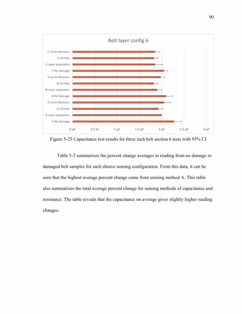
90
Figure 5-25 Capacitance test results for three inch belt section 6 tests with 95% CI
Table 5-2 summarizes the percent change averages in reading from no damage to
damaged belt samples for each sheave sensing configuration. From this data, it can be
seen that the highest average percent change came from sensing method A. This table
also summarizes the total average percent change for sensing methods of capacitance and
resistance. The table reveals that the capacitance on average gives slightly higher reading
changes.
0 pF 0.5 pF 1 pF 1.5 pF 2 pF 2.5 pF 3 pF
A‐No Damage
A‐Layer separation
A‐LS+hole
A‐LS+H+Abrasion
B‐No Damage
B‐Layer separation
B‐LS+hole
B‐LS+H+Abrasion
C‐No Damage
C‐Layer separation
C‐LS+hole
C‐LS+H+Abrasion
Belt layer config 6
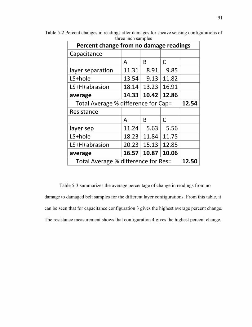
91
Table 5-2 Percent changes in readings after damages for sheave sensing configurations of three inch samples
Percent change from no damage readings
Capacitance A B C
layer separation 11.31 8.91 9.85
LS+hole 13.54 9.13 11.82
LS+H+abrasion 18.14 13.23 16.91 average 14.33 10.42 12.86
Total Average % difference for Cap= 12.54
Resistance A B C
layer sep 11.24 5.63 5.56
LS+hole 18.23 11.84 11.75
LS+H+abrasion 20.23 15.13 12.85 average 16.57 10.87 10.06
Total Average % difference for Res= 12.50
Table 5-3 summarizes the average percentage of change in readings from no
damage to damaged belt samples for the different layer configurations. From this table, it
can be seen that for capacitance configuration 3 gives the highest average percent change.
The resistance measurement shows that configuration 4 gives the highest percent change.
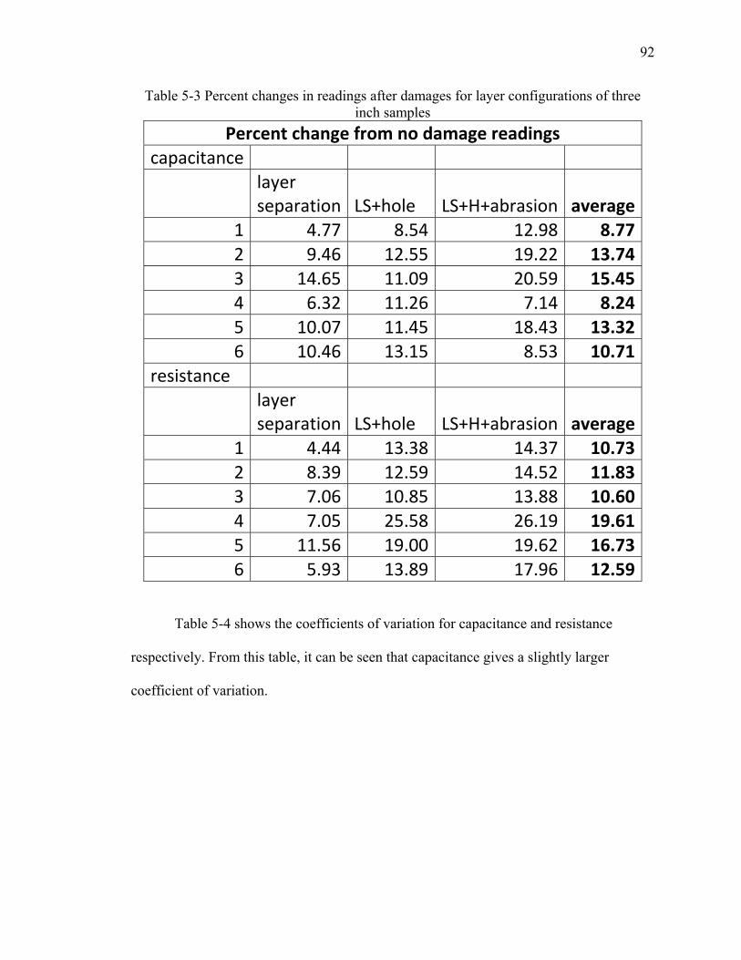
92
Table 5-3 Percent changes in readings after damages for layer configurations of three inch samples
Percent change from no damage readings
capacitance
layer separation LS+hole LS+H+abrasion average
1 4.77 8.54 12.98 8.77
2 9.46 12.55 19.22 13.74
3 14.65 11.09 20.59 15.45
4 6.32 11.26 7.14 8.24
5 10.07 11.45 18.43 13.32
6 10.46 13.15 8.53 10.71
resistance
layer separation LS+hole LS+H+abrasion average
1 4.44 13.38 14.37 10.73
2 8.39 12.59 14.52 11.833 7.06 10.85 13.88 10.60
4 7.05 25.58 26.19 19.61
5 11.56 19.00 19.62 16.73
6 5.93 13.89 17.96 12.59
Table 5-4 shows the coefficients of variation for capacitance and resistance
respectively. From this table, it can be seen that capacitance gives a slightly larger
coefficient of variation.
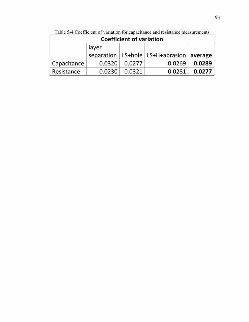
93
Table 5-4 Coefficient of variation for capacitance and resistance measurements
Coefficient of variation
layer separation LS+hole LS+H+abrasion average
Capacitance 0.0320 0.0277 0.0269 0.0289Resistance 0.0230 0.0321 0.0281 0.0277

94
CHAPTER 6. CONCLUSIONS AND RECOMMENDATIONS
6.1 Conclusions
6.1.1 Carlisle Belt Material Test Conclusions
This first set of preliminary tests gave information about the rubbers currently
used in v-belts. The exact formulations and properties of materials used by belt
manufacturers could not be disclosed directly, so the materials needed to be tested. These
results showed that the materials being used looked to be viable options for use in an
embedded capacitive sensor Smart V-Belt. The outer fabric layer did propose a hurdle
that needs to be addressed. The fabric had a lower resistance than the rubber, which
means the signal would not penetrate into the belt, but it would just travel around the belt.
Since not all belts have fabric layers, and our belt constructing process was very crude,
the fabric layer was not a part of our prototype belts. Adding a fabric layer to a belt takes
specialized tooling and an in-depth knowledge of the belt making process, neither of
which were accessible without a company partnership. The tension cords were not
included in the prototype belts for the same reasons. These tests had large standard
deviations pointing to the observation that consistency in mixing of materials in regards
to capacitance and resistance properties is not a priority for v-belt manufacturers.

95
6.1.2 Carlisle Belt Flat Plate Test Conclusions
The flat plate tests gave more evidence that the materials currently being used in
industry by Carlisle were viable options for the proposed Smart V-Belt prototypes. Many
of these flat plate tests showed very high changes in readings due to damages. The
highest being 148 percent, with many of the others in the 15-30 percent range. The 148
percent change was from 12.16pF to 30.19pF. The conclusions from the material tests
about the fabric were confirmed by the flat plate tests. The flat plate configuration 1 had
the fabric layer wrapped around the sample. This was pictured in Figure 4-26. This
configuration only had 1.55 percent change in resistance and 6.77 percent change in
capacitance for the test with only damage to the rubber. These reading changes were from
57.59kΩ to 56.65kΩ and from 13.33pF to 14.71pF respectively. This showed that the
fabric did effectively force the signal to bypass the damage within the rubber. Another
conclusion from this test was that the capacitance measurement showed much higher
percent changes than the resistance readings. It seemed that capacitance would be the
better signal to use for sensing damage within a belt. These capacitance tests were shown
through ANOVA to be significant. Tukey Comparison testing showed the data for no
damage and damage to be significantly different. These tests are shown in Appendix A.
6.1.3 Carlisle Belt Hanging Weight Test Conclusions
The testing of the Carlisle belts with the hanging weight showed the capacitance
and resistance readings did react to the amount of weight hung from the belt. The
conclusion from this was that monitoring of the belt with either resistance or capacitance
would be able to give an indication of the amount of tension. The fact that the
capacitance reaction was linearly correlated showed it to be the better parameter to use to
96
detect tension on the belt. The resistance readings seemed to have a quadratic relationship
to tension, which would be more difficult to calibrate a monitoring system. ANOVA tests
shown in Appendix B show that the data is significant. The Tukey comparison also
shows that the values for each weight are significantly different except for 10 and 20
pounds.
6.1.4 Conductive Rubber Conclusions
The conclusion of the conductive rubber tests proved that the process used was
unsuccessful in creating a reasonably consistent conductive rubber. Another observation
of this test was that the mixtures with more than 1.5 grams of carbon black did not
maintain similar material properties to the original HNBR. Those samples became brittle
because of the high amount of carbon black. These tests were ran before the shelf life of
the material was reached, but the use of this process and the 1-10 grams ratio of carbon
black to HNBR were used after the HNBR shelf life was reached. This allowed,
accidentally, for the observation of the material’s property changes from before and after
vulcanization due to time. The rubber became much more difficult to dissolve in MEK
for this mixing process. The black HNBR became even more difficult to dissolve than the
red HNBR. It was also observed through this process that the material became much
more resistant to taking the shape of the mold even under high pressure and heating.
6.1.5 Three Inch Belt Section Test Conclusions
The general trends of the measurements showed that the trend of resistance and
capacitance seem to very dependent on the type of damage and material properties. The
changes in resistance for the flat plate tests showed decreases with damage. Conversely,
the three belt section readings showed general increases in resistance due to damage.
97
Capacitance rose for the flat plate tests, while they decreased in the three inch section
tests. These baffling results are also confirmed by looking at the previous research with
these embedded sensors. Tire data showed a drop in capacitance due to damage, while O-
ring data showed increases in capacitance due to damage. This was even further
confirmed in the O-ring research, when Gallien found that some types of damages caused
increases in capacitance from the baseline, while others caused decreases in damage from
the baseline. The conclusion from these investigations has to be that in order to set cut-off
points for changes in these readings, absolute values of percent changes from baseline
must be used.
The three inch belt section data produced a conclusion concurring with the
conclusion from the flat plate tests. This conclusion was that the capacitance
measurement was a better measurement to use than resistance. The data was much clearer
in the flat plate tests. In this test, capacitance only had an average percent change 0.04
higher than resistance.
The configuration four was concluded to be not one of the optimal configurations
for sensing. The trend for the capacitance readings for this belt type were not consistent.
Some damages showed negative correlation and some positive. The coefficients of
variation for this belt were much higher than the rest of the belt configurations for
capacitance and resistance readings. The data for sensing method A was considered
insignificant because the P-value was greater than 0.05. Sensing methods B and C data
for configuration 4 had higher P-values than the other belt configurations, but were less
than 0.05. The Tukey Comparison in Appendix C also showed that almost all the values
were not significantly different at a 95 percent confidence level from the no damage to

98
damaged treatments. Only the final and most extensive damage was significantly
different for sensing methods B and C.
The optimal belt configuration strictly from the percent change data was
considered to be configuration 3 for capacitance and configuration 5 for resistance. The
optimal sheave sensing configuration strictly from the percent change data was
considered to be configuration A for capacitance and resistance. Since capacitance was
considered the better sensing parameter, the configuration 3 alone was considered to be
the overall optimal layer configuration. Belt configurations 2 and 5 were close second
and third designs from the data. After considering the confidence intervals and variation
of the data taken, belt configuration 2 was considered the optimal belt design. The
confidence intervals showed that belt configuration 2 was always significantly different
from no damage to damage. Configuration 3 was not significantly different for some
damages. The configuration 2 data also had smaller variation for both capacitance and
resistance compared to configuration 3. Sheave configuration C was a close second from
the percent difference data as well. If analyzed after deciding upon configuration 2
sensing configuration C becomes the optimal. For belt configuration 2, sensing
configuration C gives the highest R-squared value. Sensing design C was considered the
easiest to implement in a real pulley system.
6.1.6 Smart V-Belt Research Conclusions
The overall conclusion from this research of Smart V-Belts is that the concept of
an embedded capacitive sensor in a v-belt is a viable and promising concept. The high
correlation between hanging weight and capacitance readings indicated tension should be
able to be detected. The tension is likely to only be able to be read in a static state. The
99
percent change in capacitance readings from before and after damage in the flat plate
tests and three inch belt section tests show that the concept can in-fact detect damage.
The average percent changes in capacitance of 29.26 percent in the flat plate tests and
12.54 percent in the three inch belt section tests are similar to the changes in previous
research in this area. With this embedded sensor in the V-belt, the early signs of failure
should be able to be detected based on these values of change due to synthesized damage.
6.2 Recommendations
6.2.1 Additional Testing and Research
Additional testing of these most optimal sheave designs and belt layer
configurations is needed. The belt layer configurations need to be used to build full belt
prototypes. Once these belts are created, the top sheave designs can be used for testing
the belt and sheave design readings before and after damages. Once these full belts are
built, many other tests could be run on them. A test on the belt’s capacitance change due
to pulley tensioning should be conducted. Tests to reveal the change in capacitance
readings of the belts due to temperature changes should be conducted. Along with the
temperature change research, the ability to detect slippage through the heat generation
should be checked. Capacitive reaction to the introduction of different chemicals to the
belts should also be investigated.
Additional research on the optimal material properties for the construction of
these belts is needed. A dielectric material with the highest possible dielectric constant,
while maintaining the physical properties needed for v-belts, needs to be researched. A
conductive material with the physical properties needed for v-belts and the highest
possible conductance also needs to be researched. Optimizing these materials should

100
make the embedded capacitive sensor more like an ideal capacitor which would increase
the capacitor’s sensitivity to changes in these properties.
A technology that needs to be researched and possibly applied to Smart V-Belts is
wireless technology. Wireless technology built into these belts would take away the need
for sheave sensing designs and allow the belt to be a stand-alone sensor.
6.2.2 Full Data Acquisition System
A data acquisition system is needed to easily capture data from the pulley test
stand at operational speed. A full data acquisition system for this system was designed for
a project in a data acquisition class. The final presentation PowerPoint describing this
data acquisition system from class is attached as an appendix.

101
BIBLIOGRAPHY

101
BIBLIOGRAPHY
(2006). In L. Chang, Foundation of MEMS (pp. 207-240). Upper Saddle River, NJ:
Pearson/Prentice Hall.
Alberg, A. (2010). Capacitance Models of a Polymer Sealing Structure. West Lafayette,
IN: Purdue University.
Baranwal, K. C. (2001). Basic Elastomer Technology. Akron, OH: The Rubber Division,
American Chemical Society.
Belarus, T. I. (2014). V-Belt Specs. Retrieved May 2014, from VBELTS4LESS.COM:
http://www.vbelts4less.com/V-Belt-Specs_ep_45.html
Bridgestone. (2015, 1 26). Bridgestone Develops Conveyor Belt Wear Monitoring
System. Retrieved January 2015, from Bridgestone:
http://www.bridgestone.com/corporate/news/2015012601.html
Brown, R. (2012). The development of an electronic system to continually. Retrieved
January 2015, from IOP Science: http://iopscience.iop.org/1742-
6596/364/1/012055/pdf/1742-6596_364_1_012055.pdf
Brune, A. (2009). Feasibility Analysis of Utilizing a Capacitive Sensor to Detect Failure
in Lumbar Total Disc Replacements. West Lafayette, IN: Purdue University.
Carlisle, P. T. (2007). Resource Library. Retrieved July 2013, from B&B Manufacturing:
www.bbman.com/assets/files/pdf.../VBelt%20Service%20Manual.pdf

102
Continental. (2014). Conti-Protect Conti-inspect High-Performance Belt Monitoring
Systems. Retrieved January 2015, from
http://www.contitech.de/pages/produkte/transportbaender/brochures/WT9015_Co
nti-Protect_Inspect_en.pdf
Deckard, A. (2004). Life Sensing Hydraulic Hose. West Lafayette, IN: Purdue
University.
Dr. Krutz, G., Dr. Timu, G., Dr. Brittany, N., & Frank , S. (2013 ). DESIGN AND
EVALUATION OF AN EMBEDDED SENSOR IN A. Symposium on Fluid
Power & Motion Control, 1-6.
Electronics, S. (n.d.). Industrial Belt Monitoring. Retrieved January 2015, from Schrader
Electronics: https://www.schraderinternational.com/Products/Product-Folder/SA-
Industrial-Belt-Monitoring?sc_lang=en-US-SA
Engineer's Edge. (2009, Aug 25). Ohm's Law. Retrieved Oct 17, 2014, from Engineer's
Edge :
http://www.engineersedge.com/engineering/Engineering_Terms_Glossary/O/ohm
s_law_4038.htm
Engineer's Edge. (2014). Wheatstone Bridge Circuit Equations and Derivation. Retrieved
October 17, 2014, from Engineer's Edge:
http://www.engineersedge.com/instrumentation/wheat_stone_bridge.htm
Gallien, T. (2008). Design and Evaluation of an Embedded Sensor in a Polymer Sealing
Structure. West Lafayette, IN: Purdue University.
Gates, C. (n.d.). Retrieved July 26, 2013, from Gates.com:
http://www.gates.com/cool/images/V-Belt_Failure[1].pdf

103
Gerdeen, J. C. (2006). Engineering Design with Polymers and Composites. Boca Raton,
FL: Taylor & Francis Group.
Gibbins, P. (2013, 07 20). V-belt rubber information. (K. Mosier, Interviewer)
Guard, B. (n.d.). Belt Guard® Conveyor Belt Monitoring and Condition Monitoring
Systems. Retrieved January 2015, from Belt Gaurd: http://www.beltscan.com/
Holland, M. (2007). The Testing and Analysis of a Tire Response System. West Lafayette:
Purdue University.
Holland, Z. (2010). Applicataion of Electroactive polymer actuator materials in layered
polymer structures. West Lafayette, IN: Purdue University.
Honeywell. (2012, October). BeltAIS cover defect monitoring system. Retrieved January
2015, from Honeywell process solutions:
https://www.honeywellprocess.com/library/marketing/notes/PIN-
BeltAIS%20Cover-Defect-Monitoring.pdf
Insultab. (n.d.). VT-1100. Retrieved March 31, 2015, from Insultab.com:
http://www.insultab.com/vt1100-heat-gun.pdf
Klingender, R. C. (2008). Handbook of Specialty Elastomers. Boca Raton, FL: Taylor &
Francis Group.
Knies, G. (2015). High Pressure LifeSense Hydraulic Hose. Purdue University.
Krutz, G., Harmeyer, K., & Holland, M. (2005). United States of America Patent No.
US7752904.
Newell, B. (2013, June 14). Ideas for v-belt adhesives and sensing designs. (K. Mosier,
Interviewer)

104
Ohm, R. F. (1990). The Vanderbilt Rubber Handbook. Norwalk, CT: Vanderbilt
Company, Inc.
Products, A. S. (n.d.). Operator's Manual Ovens DN 42 DN 62. Mcgaw Park, Illinois,
United States of America.
Regelgerate, O. (n.d.). Electronic V-belt monitoring device. Retrieved January 2015, from
http://shop.sigstu.com/out/media/datenblatt-10103_en.pdf
Scientific, T. (2010). MaxQ 400 Incubated and refrigerated Shakers Operating Manual
and Parts List. Retrieved from Thermoscientific.com:
http://www.thermoscientific.com/content/dam/tfs/LPG/LED/LED%20Documents
/Product%20Manuals%20&%20Specifications/Shakers/Shakers/D01197~.pdf
Technologies, A. (2003). Agilent 4263B LCR Meter. Japan.
Technology, A. (n.d.). Daisy II Incubator Operator's Manual. Retrieved March 30, 2015,
from Ankom.com:
https://ankom.com/media/documents/D200_D200I_MANUAL_REV_B_101713.
Tele. (n.d.). V-Belt Monitoring. Retrieved January 2015, from Teke-online:
http://www.tele-online.com/en/case-studies/v-belt-monitoring/
Vulcanization. (2014, 2 3). Retrieved 2 2, 2015, from Encylopedia:
http://www.britannica.com/EBchecked/topic/633433/vulcanization
Zhao, X., Zhang , Q., Gu, J., & Yin, D. (2011). Effects of Carbon Black on the Properties
of HNBR. Polymer-Plastics Technology and Engineering, 1507-1510.

APPENDICES

105
Appendix A ANOVA and Tukey Tests for Flat Plate Data
Flat plate test 1
Source DF SS MS F P Trt 2 20.1733 10.0867 136.37 0.000 Error 27 1.9970 0.0740 Total 29 22.1703 S = 0.2720 R-Sq = 90.99% R-Sq(adj) = 90.33%
Grouping Information Using Tukey Method Trt N Mean Grouping Hole_fabric 10 15.2840 A Hole_rubber 10 14.7100 B Control 10 13.3300 C Means that do not share a letter are significantly different. Tukey 95% Simultaneous Confidence Intervals All Pairwise Comparisons among Levels of Trt
Flat plate test 2
Source DF SS MS F P Trt 1 8.97800 8.97800 1346.70 0.000 Error 18 0.12000 0.00667 Total 19 9.09800 S = 0.08165 R-Sq = 98.68% R-Sq(adj) = 98.61%
Grouping Information Using Tukey Method Trt N Mean Grouping Control 10 10.2800 A Hole_rubber 10 8.9400 B Means that do not share a letter are significantly different. Tukey 95% Simultaneous Confidence Intervals All Pairwise Comparisons among Levels of Trt
Flat plate test 3
Source DF SS MS F P Trt 2 1794.413 897.206 1776.39 0.000 Error 27 13.637 0.505 Total 29 1808.050
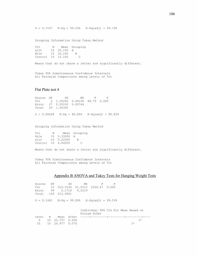
106
S = 0.7107 R-Sq = 99.25% R-Sq(adj) = 99.19%
Grouping Information Using Tukey Method Trt N Mean Grouping slit 10 30.190 A Hole 10 16.140 B Control 10 12.160 C Means that do not share a letter are significantly different. Tukey 95% Simultaneous Confidence Intervals All Pairwise Comparisons among Levels of Trt
Flat Plate test 4
Source DF SS MS F P Trt 2 1.32200 0.66100 88.79 0.000 Error 27 0.20100 0.00744 Total 29 1.52300 S = 0.08628 R-Sq = 86.80% R-Sq(adj) = 85.82%
Grouping Information Using Tukey Method Trt N Mean Grouping Hole 10 5.33000 A slit 10 5.22000 B Control 10 4.84000 C Means that do not share a letter are significantly different. Tukey 95% Simultaneous Confidence Intervals All Pairwise Comparisons among Levels of Trt
Appendix B ANOVA and Tukey Tests for Hanging Weight Tests
Source DF SS MS F P Trt 10 510.3146 51.0315 2326.47 0.000 Error 99 2.1716 0.0219 Total 109 512.4861 S = 0.1481 R-Sq = 99.58% R-Sq(adj) = 99.53% Individual 95% CIs For Mean Based on Pooled StDev Level N Mean StDev -----+---------+---------+---------+---- 0 10 25.757 0.094 (* 10 10 24.977 0.070 (*
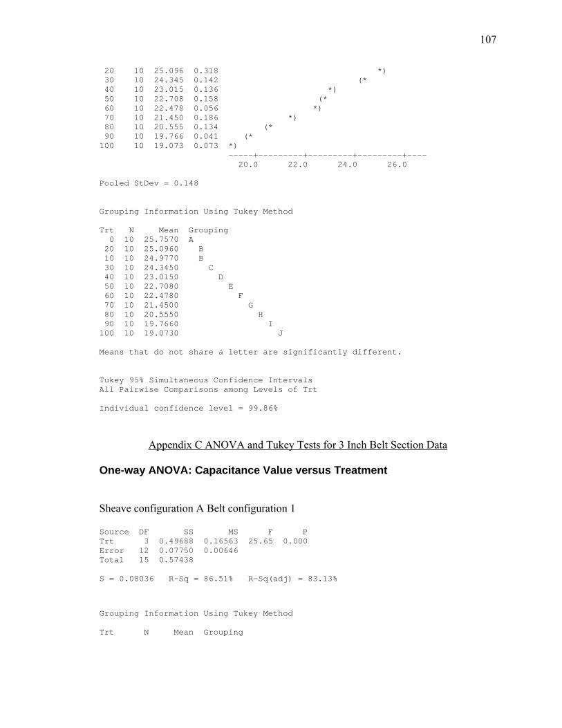
107
20 10 25.096 0.318 *) 30 10 24.345 0.142 (* 40 10 23.015 0.136 *) 50 10 22.708 0.158 (* 60 10 22.478 0.056 *) 70 10 21.450 0.186 *) 80 10 20.555 0.134 (* 90 10 19.766 0.041 (* 100 10 19.073 0.073 *) -----+---------+---------+---------+---- 20.0 22.0 24.0 26.0 Pooled StDev = 0.148 Grouping Information Using Tukey Method Trt N Mean Grouping 0 10 25.7570 A 20 10 25.0960 B 10 10 24.9770 B 30 10 24.3450 C 40 10 23.0150 D 50 10 22.7080 E 60 10 22.4780 F 70 10 21.4500 G 80 10 20.5550 H 90 10 19.7660 I 100 10 19.0730 J Means that do not share a letter are significantly different. Tukey 95% Simultaneous Confidence Intervals All Pairwise Comparisons among Levels of Trt Individual confidence level = 99.86%
Appendix C ANOVA and Tukey Tests for 3 Inch Belt Section Data
One-way ANOVA: Capacitance Value versus Treatment
Sheave configuration A Belt configuration 1
Source DF SS MS F P Trt 3 0.49688 0.16563 25.65 0.000 Error 12 0.07750 0.00646 Total 15 0.57438 S = 0.08036 R-Sq = 86.51% R-Sq(adj) = 83.13%
Grouping Information Using Tukey Method Trt N Mean Grouping

108
Control 4 2.37500 A Sep 4 2.20000 B Hole 4 2.05000 B C Abr 4 1.90000 C Means that do not share a letter are significantly different. Tukey 95% Simultaneous Confidence Intervals All Pairwise Comparisons among Levels of Trt
Sheave configuration A Belt configuration 2
Source DF SS MS F P Trt 3 0.23188 0.07729 33.73 0.000 Error 12 0.02750 0.00229 Total 15 0.25938 S = 0.04787 R-Sq = 89.40% R-Sq(adj) = 86.75% Grouping Information Using Tukey Method Trt N Mean Grouping Control 4 1.72500 A Sep 4 1.60000 B Hole 4 1.50000 B C Abr 4 1.40000 C Means that do not share a letter are significantly different. Tukey 95% Simultaneous Confidence Intervals All Pairwise Comparisons among Levels of Trt
Sheave configuration A Belt configuration 3
Source DF SS MS F P Trt 3 0.087500 0.029167 35.00 0.000 Error 12 0.010000 0.000833 Total 15 0.097500 S = 0.02887 R-Sq = 89.74% R-Sq(adj) = 87.18%
Grouping Information Using Tukey Method Trt N Mean Grouping Control 4 0.90000 A Hole 4 0.80000 B Sep 4 0.75000 B C Abr 4 0.70000 C Means that do not share a letter are significantly different.

109
Tukey 95% Simultaneous Confidence Intervals All Pairwise Comparisons among Levels of Trt
Sheave configuration A Belt configuration 4
Source DF SS MS F P Trt 3 0.03250 0.01083 2.89 0.079 Error 12 0.04500 0.00375 Total 15 0.07750 S = 0.06124 R-Sq = 41.94% R-Sq(adj) = 27.42%
Grouping Information Using Tukey Method Trt N Mean Grouping Control 4 0.65000 A Sep 4 0.60000 A Hole 4 0.57500 A Abr 4 0.52500 A Means that do not share a letter are significantly different. Tukey 95% Simultaneous Confidence Intervals All Pairwise Comparisons among Levels of Trt
Sheave configuration A Belt configuration 5
Source DF SS MS F P Trt 3 0.30500 0.10167 48.80 0.000 Error 12 0.02500 0.00208 Total 15 0.33000 S = 0.04564 R-Sq = 92.42% R-Sq(adj) = 90.53%
Grouping Information Using Tukey Method Trt N Mean Grouping Control 4 1.90000 A Sep 4 1.65000 B Hole 4 1.62500 B Abr 4 1.52500 C Means that do not share a letter are significantly different. Tukey 95% Simultaneous Confidence Intervals All Pairwise Comparisons among Levels of Trt
Sheave configuration A Belt configuration 6

110
Source DF SS MS F P Trt 3 0.27250 0.09083 12.82 0.000 Error 12 0.08500 0.00708 Total 15 0.35750 S = 0.08416 R-Sq = 76.22% R-Sq(adj) = 70.28%
Grouping Information Using Tukey Method Trt N Mean Grouping Control 4 2.27500 A Abr 4 2.05000 B Sep 4 2.00000 B Hole 4 1.92500 B Means that do not share a letter are significantly different. Tukey 95% Simultaneous Confidence Intervals All Pairwise Comparisons among Levels of Trt Individual confidence level = 98.83%
Sheave configuration B Belt configuration 1
Source DF SS MS F P Trt 3 0.51188 0.17063 63.00 0.000 Error 12 0.03250 0.00271 Total 15 0.54438 S = 0.05204 R-Sq = 94.03% R-Sq(adj) = 92.54%
Grouping Information Using Tukey Method Trt N Mean Grouping Control 4 2.37500 A Sep 4 2.15000 B Hole 4 2.07500 B Abr 4 1.87500 C Means that do not share a letter are significantly different. Tukey 95% Simultaneous Confidence Intervals All Pairwise Comparisons among Levels of Trt
Sheave configuration B Belt configuration 2
Source DF SS MS F P Trt 3 0.32187 0.10729 34.33 0.000 Error 12 0.03750 0.00313 Total 15 0.35937

111
S = 0.05590 R-Sq = 89.57% R-Sq(adj) = 86.96% Grouping Information Using Tukey Method Trt N Mean Grouping Control 4 2.05000 A Sep 4 1.85000 B Hole 4 1.82500 B Abr 4 1.65000 C Means that do not share a letter are significantly different. Tukey 95% Simultaneous Confidence Intervals All Pairwise Comparisons among Levels of Trt
Sheave configuration B Belt configuration 3
Source DF SS MS F P Trt 3 0.08750 0.02917 11.67 0.001 Error 12 0.03000 0.00250 Total 15 0.11750 S = 0.05 R-Sq = 74.47% R-Sq(adj) = 68.09%
Grouping Information Using Tukey Method Trt N Mean Grouping Control 4 0.97500 A Hole 4 0.87500 A B Sep 4 0.82500 B Abr 4 0.77500 B Means that do not share a letter are significantly different. Tukey 95% Simultaneous Confidence Intervals All Pairwise Comparisons among Levels of Trt
Sheave configuration B Belt configuration 4
Source DF SS MS F P Trt 3 0.09500 0.03167 5.85 0.011 Error 12 0.06500 0.00542 Total 15 0.16000 S = 0.07360 R-Sq = 59.38% R-Sq(adj) = 49.22%
Grouping Information Using Tukey Method Trt N Mean Grouping Abr 4 0.77500 A Control 4 0.65000 A B Sep 4 0.60000 B Hole 4 0.57500 B

112
Means that do not share a letter are significantly different. Tukey 95% Simultaneous Confidence Intervals All Pairwise Comparisons among Levels of Trt
Sheave configuration B Belt configuration 5
Source DF SS MS F P Trt 3 0.21250 0.07083 34.00 0.000 Error 12 0.02500 0.00208 Total 15 0.23750 S = 0.04564 R-Sq = 89.47% R-Sq(adj) = 86.84%
Grouping Information Using Tukey Method Trt N Mean Grouping Control 4 1.70000 A Sep 4 1.55000 B Hole 4 1.52500 B Abr 4 1.37500 C Means that do not share a letter are significantly different. Tukey 95% Simultaneous Confidence Intervals All Pairwise Comparisons among Levels of Trt
Sheave configuration B Belt configuration 6
Source DF SS MS F P Trt 3 0.16500 0.05500 18.86 0.000 Error 12 0.03500 0.00292 Total 15 0.20000 S = 0.05401 R-Sq = 82.50% R-Sq(adj) = 78.13% Grouping Information Using Tukey Method Trt N Mean Grouping Control 4 2.10000 A Abr 4 1.97500 B Sep 4 1.90000 B C Hole 4 1.82500 C Means that do not share a letter are significantly different. Tukey 95% Simultaneous Confidence Intervals All Pairwise Comparisons among Levels of Trt
Sheave configuration C Belt configuration 1

113
Source DF SS MS F P Trt 3 0.53187 0.17729 31.52 0.000 Error 12 0.06750 0.00563 Total 15 0.59937 S = 0.075 R-Sq = 88.74% R-Sq(adj) = 85.92%
Grouping Information Using Tukey Method Trt N Mean Grouping Control 4 2.50000 A Sep 4 2.30000 B Hole 4 2.17500 B Abr 4 2.00000 C Means that do not share a letter are significantly different. Tukey 95% Simultaneous Confidence Intervals All Pairwise Comparisons among Levels of Trt Individual confidence level = 98.83%
Sheave configuration C Belt configuration 2
Source DF SS MS F P Trt 3 0.38188 0.12729 87.29 0.000 Error 12 0.01750 0.00146 Total 15 0.39938 S = 0.03819 R-Sq = 95.62% R-Sq(adj) = 94.52%
Grouping Information Using Tukey Method Trt N Mean Grouping Control 4 2.20000 A Sep 4 1.95000 B Hole 4 1.90000 B Abr 4 1.77500 C Means that do not share a letter are significantly different. Tukey 95% Simultaneous Confidence Intervals All Pairwise Comparisons among Levels of Trt
Sheave configuration C Belt configuration 3
Source DF SS MS F P Trt 3 0.08250 0.02750 9.43 0.002 Error 12 0.03500 0.00292 Total 15 0.11750

114
S = 0.05401 R-Sq = 70.21% R-Sq(adj) = 62.77%
Grouping Information Using Tukey Method Trt N Mean Grouping Control 4 1.05000 A Sep 4 0.92500 B Hole 4 0.92500 B Abr 4 0.85000 B Means that do not share a letter are significantly different. Tukey 95% Simultaneous Confidence Intervals All Pairwise Comparisons among Levels of Trt
Sheave configuration C Belt configuration 4
Source DF SS MS F P Trt 3 0.11250 0.03750 6.92 0.006 Error 12 0.06500 0.00542 Total 15 0.17750 S = 0.07360 R-Sq = 63.38% R-Sq(adj) = 54.23%
Grouping Information Using Tukey Method Trt N Mean Grouping Abr 4 0.85000 A Control 4 0.70000 A B Sep 4 0.67500 B Hole 4 0.62500 B Means that do not share a letter are significantly different. Tukey 95% Simultaneous Confidence Intervals All Pairwise Comparisons among Levels of Trt
Sheave configuration C Belt configuration 5
Source DF SS MS F P Trt 3 0.18188 0.06063 22.38 0.000 Error 12 0.03250 0.00271 Total 15 0.21438 S = 0.05204 R-Sq = 84.84% R-Sq(adj) = 81.05%
Grouping Information Using Tukey Method

115
Trt N Mean Grouping Control 4 1.82500 A Sep 4 1.67500 B Hole 4 1.65000 B Abr 4 1.52500 C Means that do not share a letter are significantly different. Tukey 95% Simultaneous Confidence Intervals All Pairwise Comparisons among Levels of Trt
Sheave configuration C Belt configuration 6
Source DF SS MS F P Trt 3 0.13187 0.04396 14.07 0.000 Error 12 0.03750 0.00312 Total 15 0.16937 S = 0.05590 R-Sq = 77.86% R-Sq(adj) = 72.32%
Grouping Information Using Tukey Method Trt N Mean Grouping Control 4 2.05000 A Sep 4 1.85000 B Abr 4 1.85000 B Hole 4 1.82500 B Means that do not share a letter are significantly different. Tukey 95% Simultaneous Confidence Intervals All Pairwise Comparisons among Levels of Trt

116
Appendix D Material Data and Safety Sheets
Figure D-1 Original Kirkhill Black HNBR Data Sheet Page 1
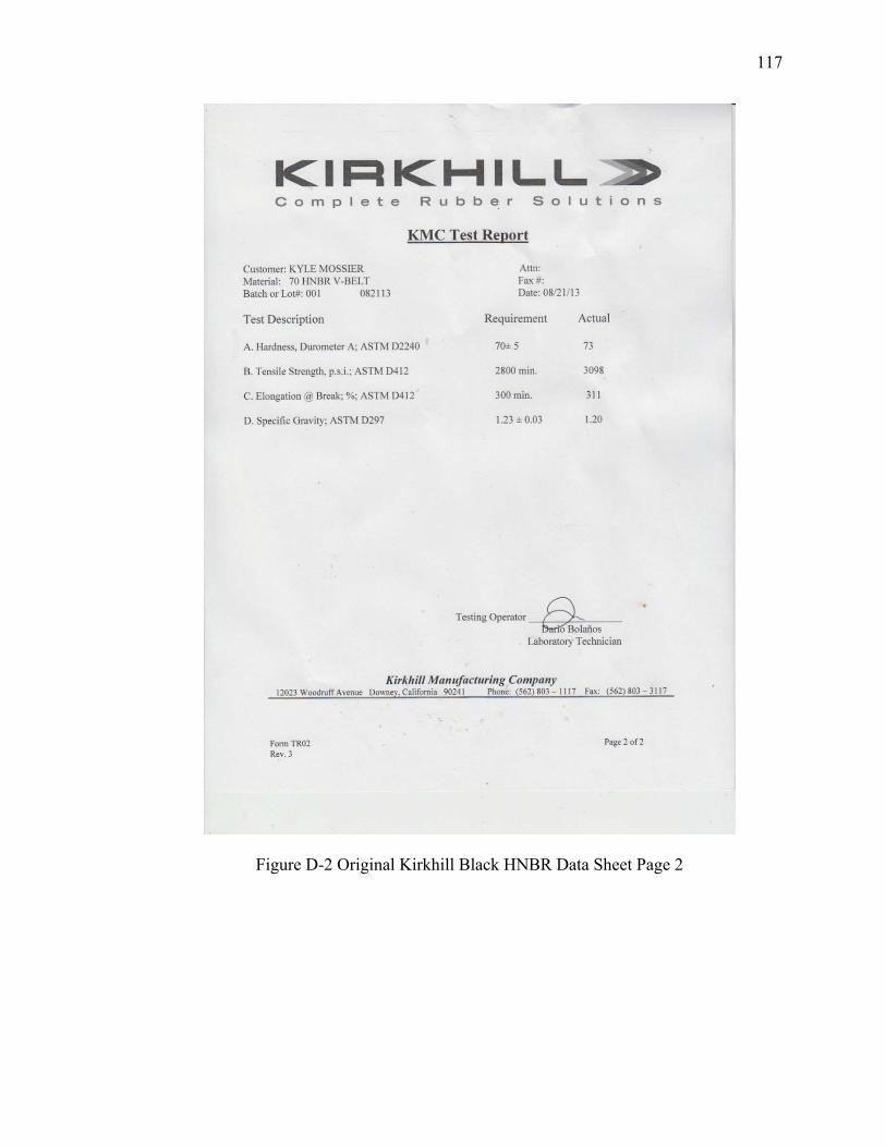
117
Figure D-2 Original Kirkhill Black HNBR Data Sheet Page 2
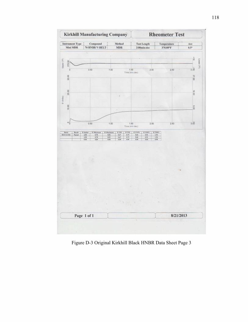
118
Figure D-3 Original Kirkhill Black HNBR Data Sheet Page 3
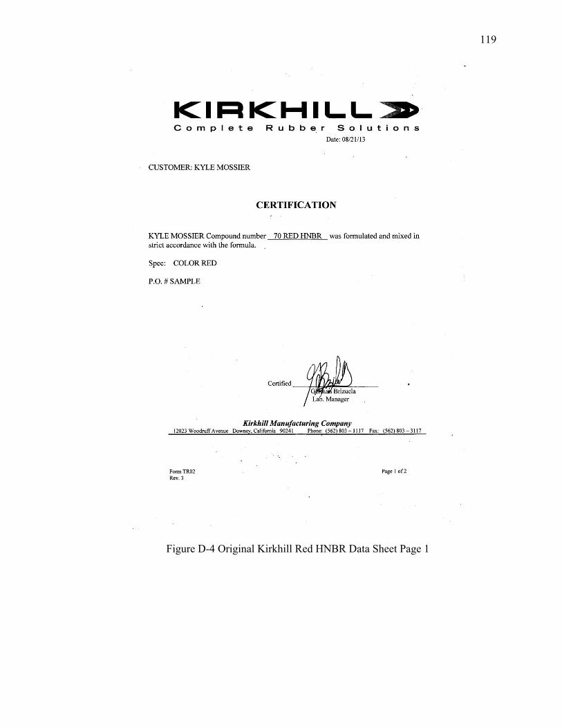
119
Figure D-4 Original Kirkhill Red HNBR Data Sheet Page 1
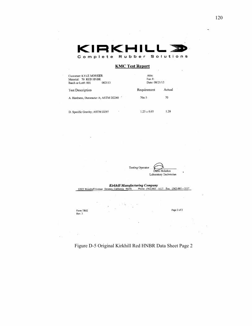
120
Figure D-5 Original Kirkhill Red HNBR Data Sheet Page 2
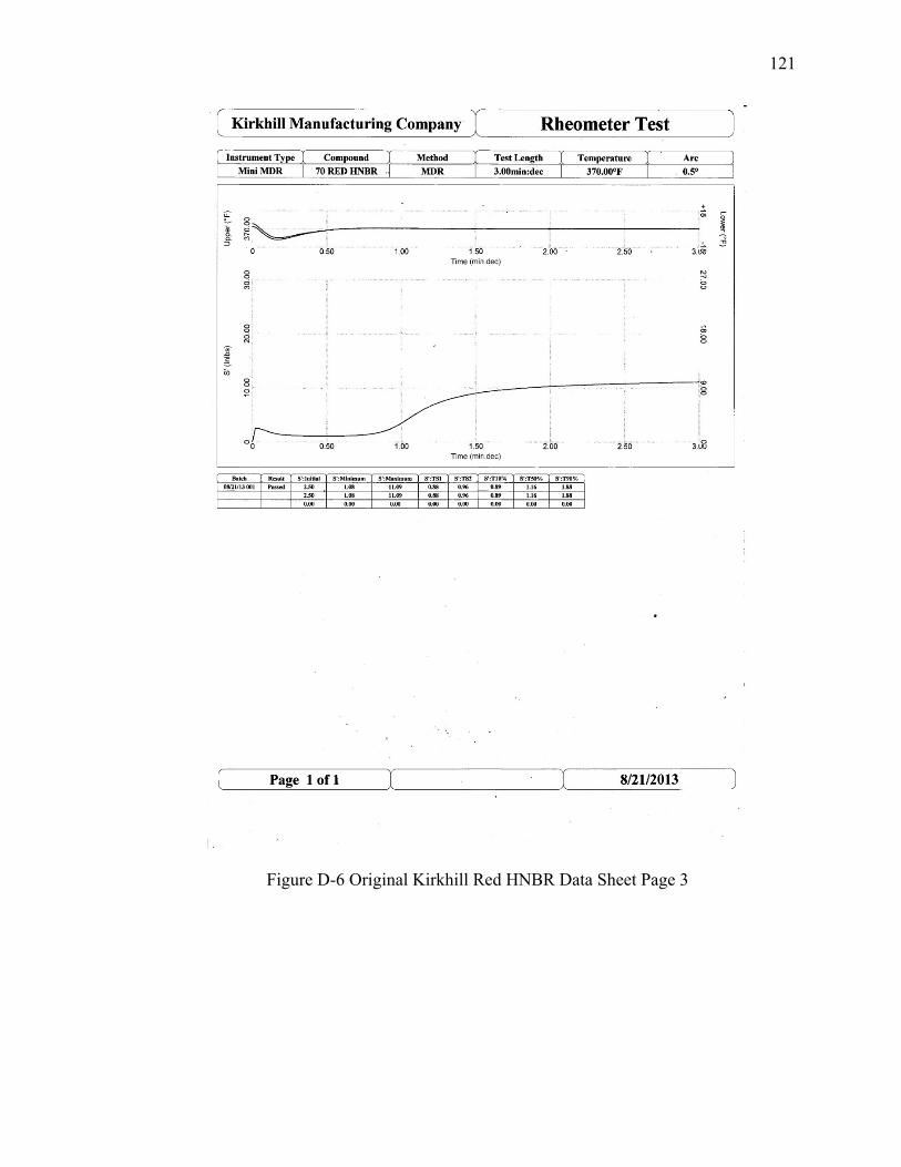
121
Figure D-6 Original Kirkhill Red HNBR Data Sheet Page 3

122
Figure D-7 New Kirkhill Black HNBR Data Sheet Page 1
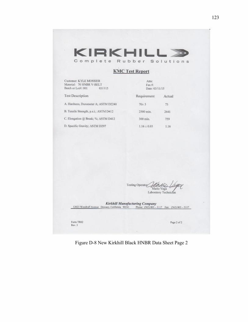
123
Figure D-8 New Kirkhill Black HNBR Data Sheet Page 2
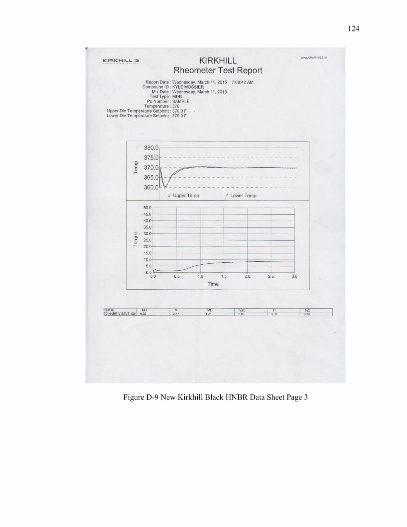
124
Figure D-9 New Kirkhill Black HNBR Data Sheet Page 3
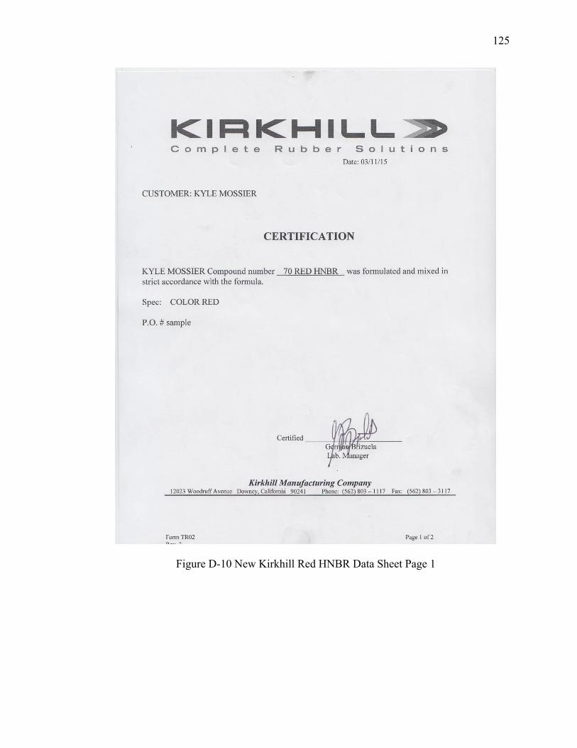
125
Figure D-10 New Kirkhill Red HNBR Data Sheet Page 1
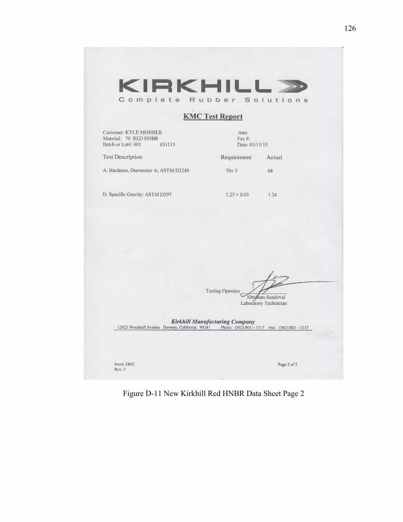
126
Figure D-11 New Kirkhill Red HNBR Data Sheet Page 2
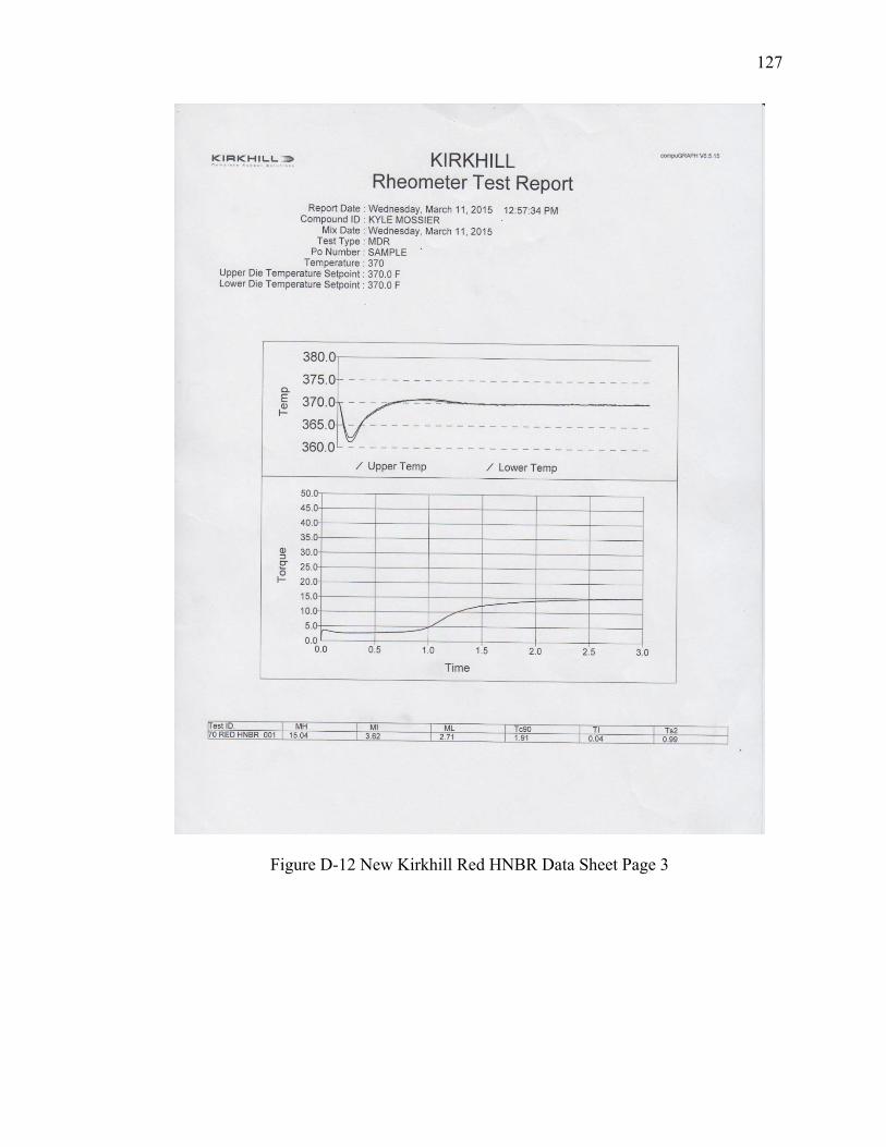
127
Figure D-12 New Kirkhill Red HNBR Data Sheet Page 3
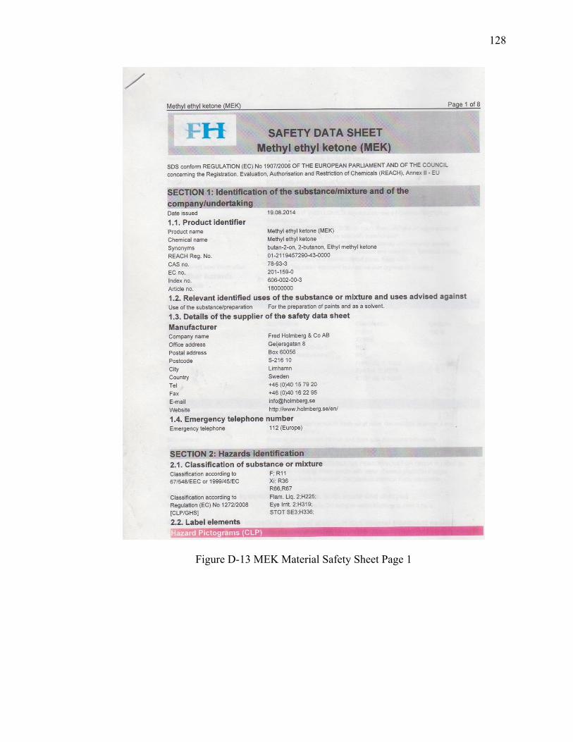
128
Figure D-13 MEK Material Safety Sheet Page 1
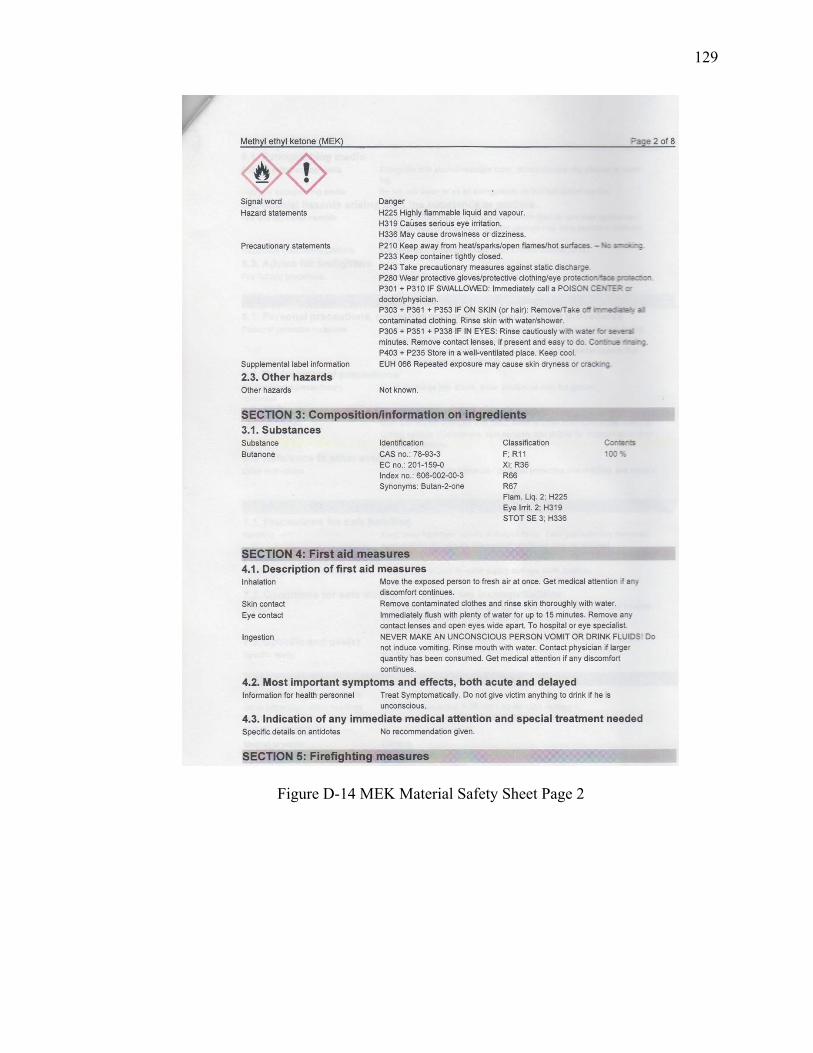
129
Figure D-14 MEK Material Safety Sheet Page 2

130
Figure D-15 MEK Material Safety Sheet Page 3
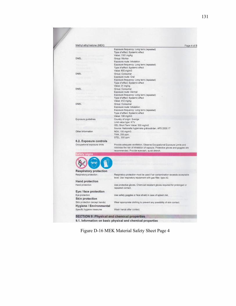
131
Figure D-16 MEK Material Safety Sheet Page 4
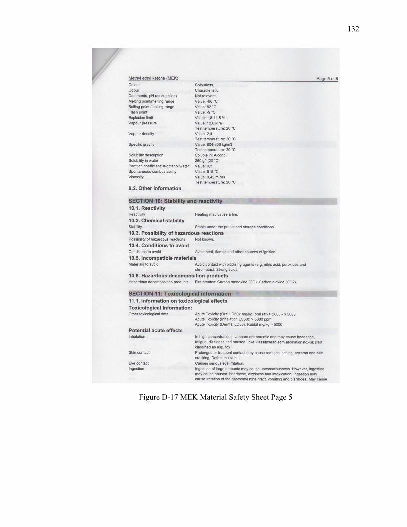
132
Figure D-17 MEK Material Safety Sheet Page 5
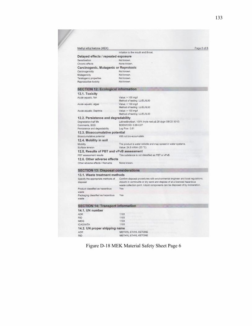
133
Figure D-18 MEK Material Safety Sheet Page 6
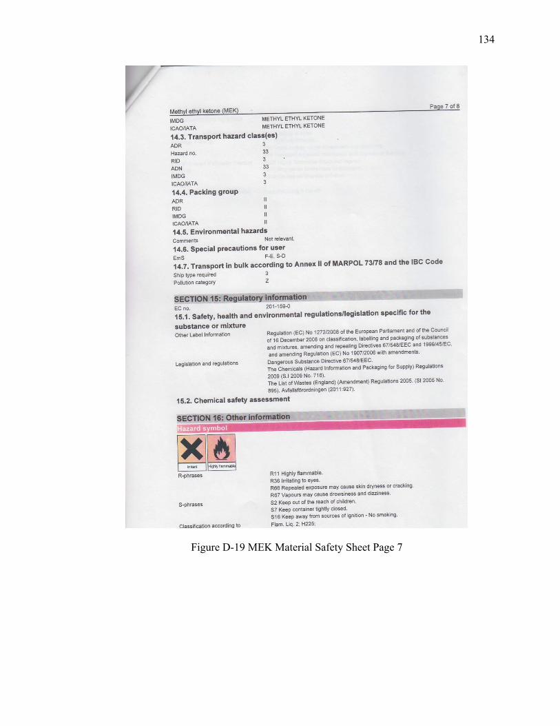
134
Figure D-19 MEK Material Safety Sheet Page 7
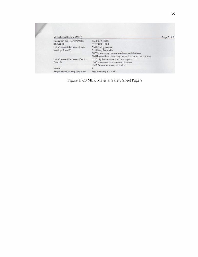
135
Figure D-20 MEK Material Safety Sheet Page 8
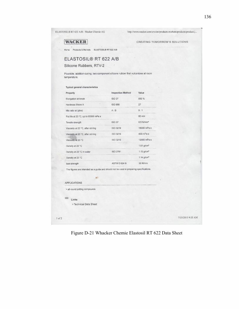
136
Figure D-21 Whacker Chemie Elastosil RT 622 Data Sheet
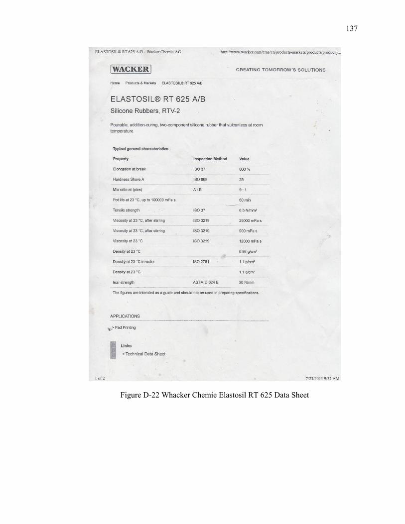
137
Figure D-22 Whacker Chemie Elastosil RT 625 Data Sheet
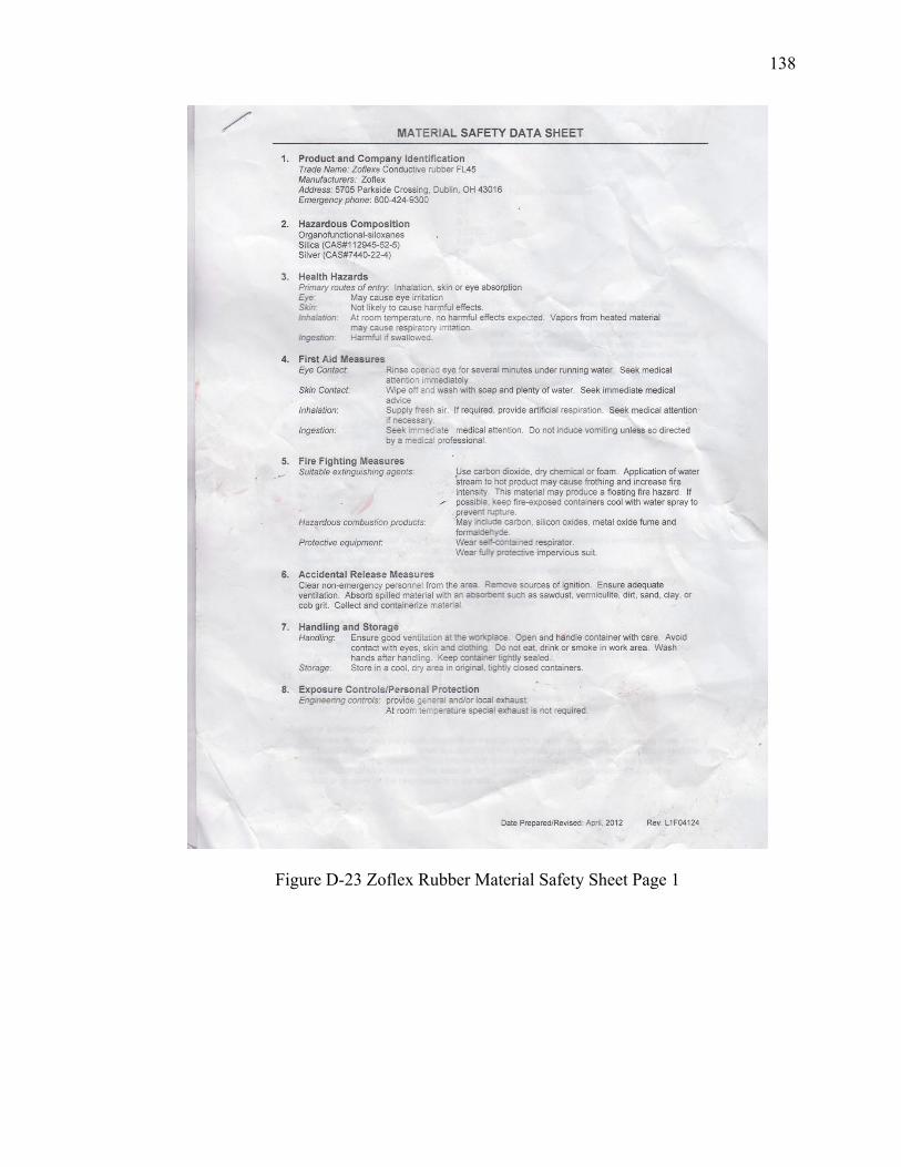
138
Figure D-23 Zoflex Rubber Material Safety Sheet Page 1
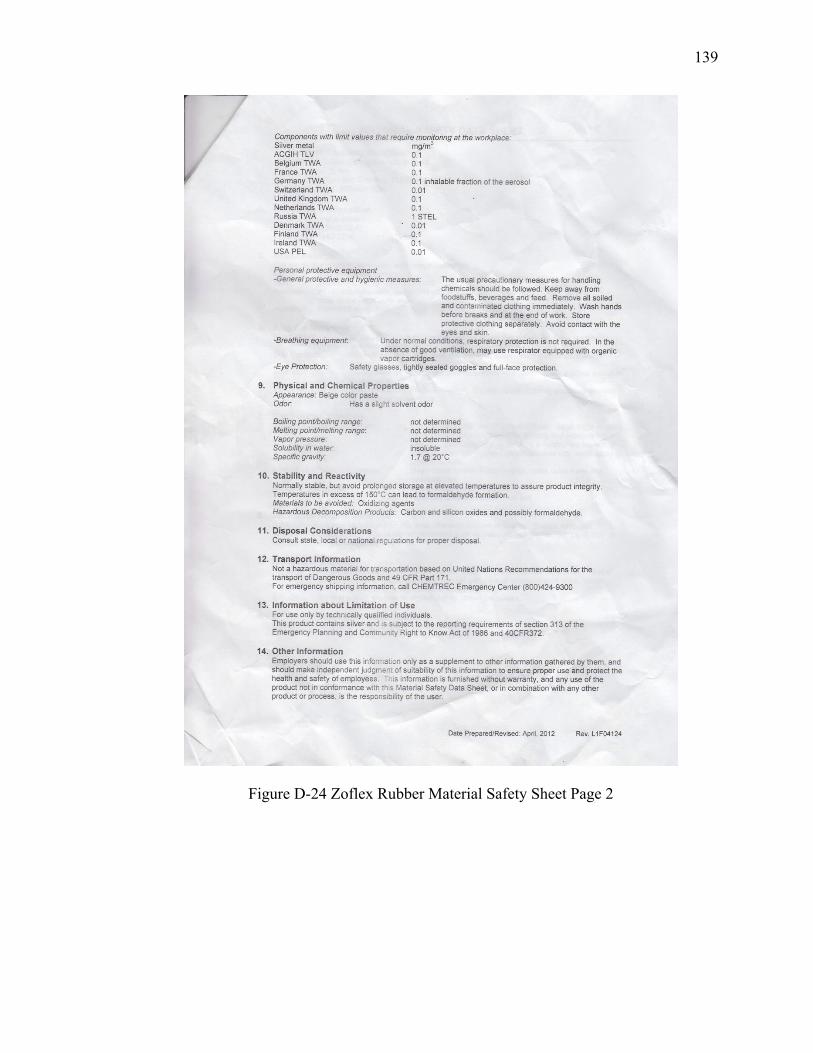
139
Figure D-24 Zoflex Rubber Material Safety Sheet Page 2
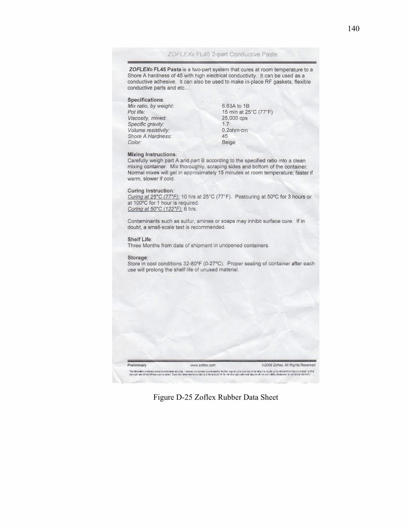
140
Figure D-25 Zoflex Rubber Data Sheet
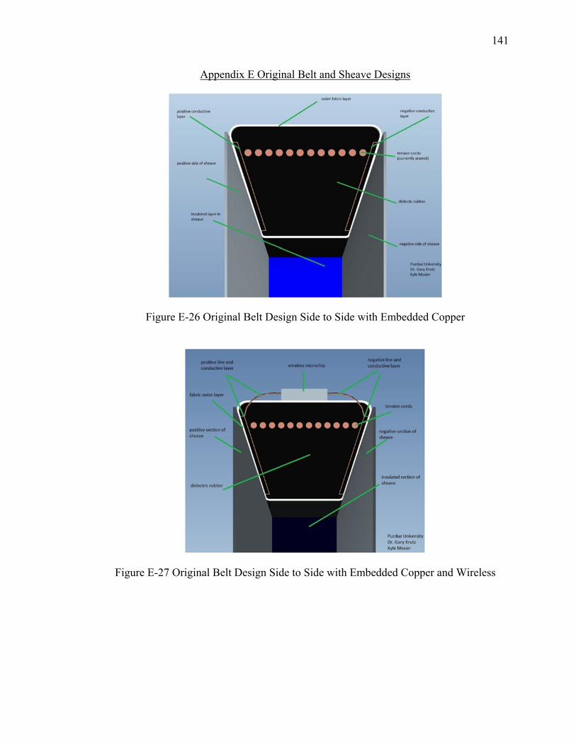
141
Appendix E Original Belt and Sheave Designs
Figure E-26 Original Belt Design Side to Side with Embedded Copper
Figure E-27 Original Belt Design Side to Side with Embedded Copper and Wireless
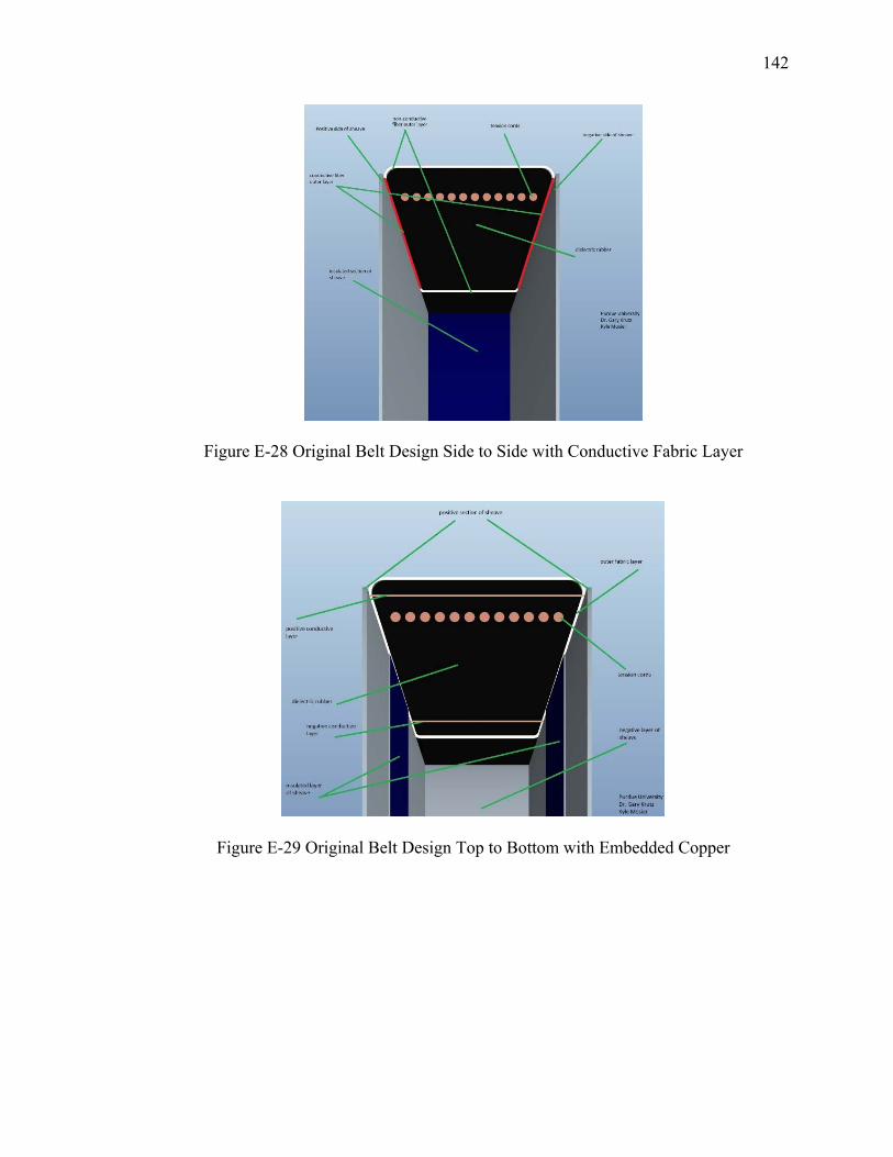
142
Figure E-28 Original Belt Design Side to Side with Conductive Fabric Layer
Figure E-29 Original Belt Design Top to Bottom with Embedded Copper
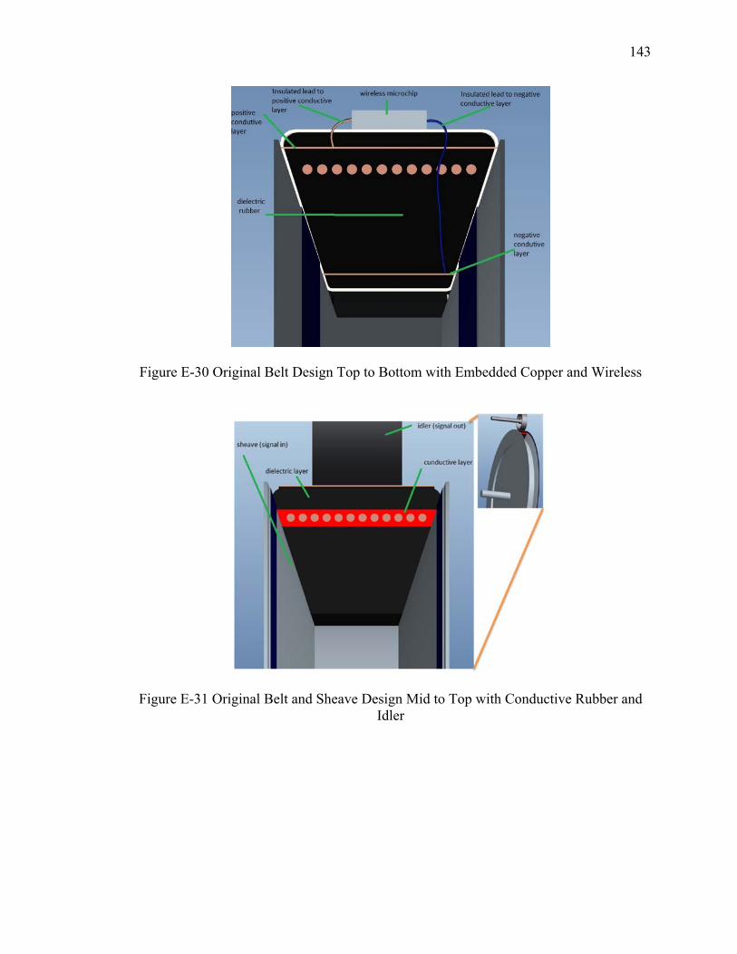
143
Figure E-30 Original Belt Design Top to Bottom with Embedded Copper and Wireless
Figure E-31 Original Belt and Sheave Design Mid to Top with Conductive Rubber and Idler
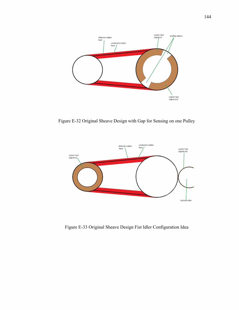
144
Figure E-32 Original Sheave Design with Gap for Sensing on one Pulley
Figure E-33 Original Sheave Design Fist Idler Configuration Idea
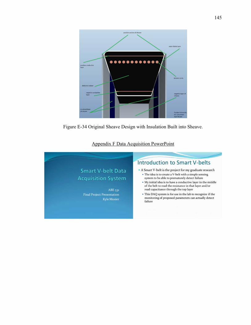
145
Figure E-34 Original Sheave Design with Insulation Built into Sheave.
Appendix F Data Acquisition PowerPoint
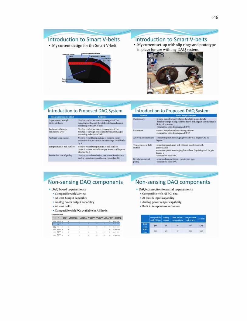
146
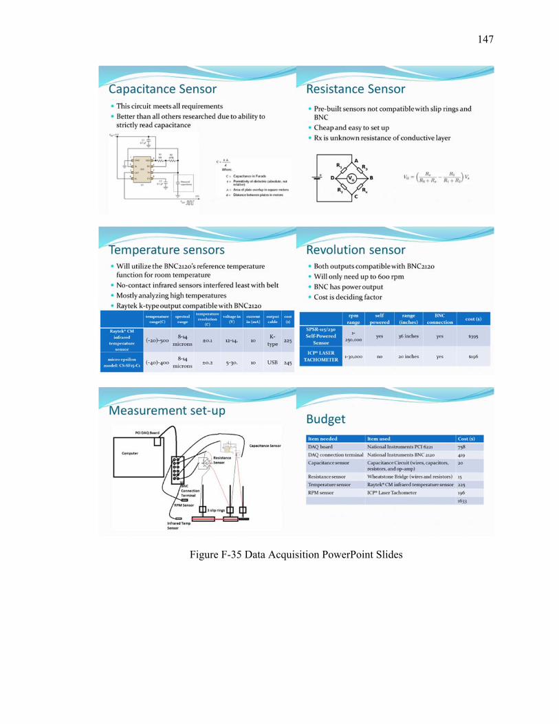
147
Figure F-35 Data Acquisition PowerPoint Slides