Embed Size (px)
Citation preview

Technische Universit�at Wien
DISSERTATION
Smart Antennasfor Second and Third GenerationMobile Communications Systems
ausgef�uhrt zum Zwecke der Erlangung des akademischen Grades einesDoktors der technischen Wissenschaften unter der Leitung von
Prof. Dipl.{Ing. Dr. Ernst BONEK
E 389Institut f�ur Nachrichtentechnik und Hochfrequenztechnik
eingereicht an der
Technischen Universit�at WienFakult�at f�ur Elektrotechnik
von
Dipl.{Ing. Mag. Josef FUHL
Matrikelnummer 8825568
A{2803 Schwarzenbach, Eggenbuch 17geboren in Schwarzenbach am 05. Februar 1968
Wien, im M�arz 1997 . . . . . . . . . . . . . . . . . . . . . . . . . . . . . . . . . . . . . .


to my parents

Acknowledgment
I am deeply grateful to Prof. Ernst Bonek for having initiated the research co{operationbetween the institute and the PTA (Post & Telekom Austria) on smart antennas, for hisavailability whenever questions arised, for his continuous support and encouragement duringthe course of this work, and for various suggestions improving the quality of this thesis.
My gratitude also goes to Prof. Paul Walter Baier for critical reading of the manuscriptand many useful suggestions.
I am grateful to Post & Telekom Austria who made possible this work by a generousgrant, for the scienti�c freedom, and for the ability to publish results freely.
My great appreciation goes to my colleagues Gerhard Schultes, Hermann B�uhler, RainerGahleitner, Peter Kreuzgruber, Norbert Rohringer, Walter Sch�uttengruber, Martin Hage-nauer, Paulina Eratuli, Juha Laurila, Wolfgang Konrad, and Heinz Novak for their fruitfulcollaboration.
Special thanks go to Alexander Kuchar, Andreas Molisch, and Markus Uhlirz for manycritical and useful suggestions and discussions, and for carefully reading the �rst draft of themanuscript.
I want to express my thanks to the research groups of Prof. P. W. Baier, Prof. J. A.Nossek, and to Utz Martin from Deutsche Telekom and Martin Tangemann form Alcatel SELAG for helpful discussions.
I owe special thanks to Tomas Cichon, Universit�at Karlsruhe, Patrick Eggers, AlborgUniversity, and Jean{Pierre Rossi, France Telecom for providing ray tracing and measurementdata for the use within this thesis.
Finally, I want to thank Claudia for her patience and understanding.
5


Zusammenfassung
Diese Arbeit untersucht ein neues Verfahren zur Erh�ohung der Kapazit�at von Mobilfunksy-stemen | Intelligente Antennen. Intelligente Antennen nutzen die Richtungsinhomogenit�atder an der Basistation eintre�enden Signale. Sie empfangen (senden) Signale nur aus (in)jene(n) Richtungen, aus welchen die gew�unschten Signalanteile an der Antenne einfallen.Dabei wird die Interferenz und die Zeitdispersion reduziert, der Versorgungsbereich vergr�o�ertund der Schwund verringert.
Ich analysiere zwei Anwendungsarten dieses Verfahrens:
� R�aumliche Filterung zur Interferenzminderung (SFIR, Spatial Filtering for InterferenceReduction): Pro Verkehrskanal wird ein Benutzer bedient. Da die Antenne nur Leistungaus den Richtungen, aus denen die gew�unschten Signale eintre�en, empf�angt, wird dieInterferenz reduziert. Daher k�onnen kleinere Clusterma�e verwendet werden, wodurchdie spektrale E�zienz und damit die Kapazit�at steigt.
� Raummultiplex (SDMA, Space Division Multiple Access): Mehrere Benutzer werdengleichzeitig in demselben Verkehrskanal bedient, was zu einer direkten Erh�ohung derspektralen E�zienz f�uhrt.
Ich untersuche die notwendigen Schritte zur Implementierung intelligenter Antennen, dassind Richtungssch�atzung, Richtdiagrammformung, Signaltrennung und Synchronisation f�urSR (Spatial Reference) Algorithmen; sowie Synchronisation und Richtdiagrammformung f�urTR (Temporal Reference) Algorithmen. Ich schlage ein Konzept zur Erweiterung von Sy-stemen der zweiten Generation (GSM, DCS 1800) mit intelligenten Antennen vor.
Der Entwurf, der Test und der Vergleich von Systemen mit intelligenten Antennen er-fordert richtungsabh�angige Kanalmodelle, daher erweitere ich die existierenden Kanalmodelleum Einfallsrichtungen und bestimme Raum- und Frequenzkorrelationskoe�zienten der ein-fallenden Signalanteile. Der Raumkorrelationskoe�zient ist gro� f�ur die �ublichen Winkelauf-spreizung der einfallenden Signale. F�ur Einfallsrichtungen '0 = 0�; 60�; und 90� (gemessenvon der Normalen zur Gruppenantennenachse) darf die maximale Winkelaufspreizung der aneiner Gruppenantenne der L�ange 5�, wobei � die Wellenl�ange ist, einfallenden Signale f�ur eineKorrelation von �env � 0:9 nicht gr�o�er als S' � 0:5�; 1�; und 10� sein. Ist der Raumkorrela-tionskoe�zient �env < 0:5, so ist die Antennenstruktur eine e�ektive Diversit�atsanordnung.
Die Frequenzkorrelation zwischen Aufw�arts{ und Abw�artsstrecke in Frequenzduplexsy-stemen, wie GSM und DCS 1800, ist sehr gering. In einem Szenario ohne direkte Sichtver-bindung zwischen Sender und Empf�anger, mit einem Radius des Streuerkreises von R = 100�,betr�agt der Frequenzunterschied zwischen Aufw�arts{ und Abw�artsstrecke f�ur einen Frequenz-korrelationskoe�zienten von ��! = 0:5 nur 0:3% der Mittenfrequenz. Der Schwund f�ur dieAufw�arts{ und Abw�artsstrecke in FDD (Frequency Division Duplex){Systemen ist daher
7

nicht korreliert. Dies beein u�t die Wahl eines geeigneten Adaptionsalgorithmus f�ur dieRichtdiagrammformung f�ur die Abw�artsstrecke.
Basierend auf diesem Kanalmodell untersuche ich das Verhalten von SR und TR Algo-rithmen sowohl f�ur die Aufw�arts- als auch f�ur die Abw�artsstrecke. Die Wahl des Algorithmush�angt entscheidend von der Umgebung der Basisstationsantenne ab. Die Gruppe der SRAlgorithmen ist die erfolgversprechendste, wenn nominelle Richtungen existieren. Das Wortnominell bedeutet, da� die Richtungen nicht diskret sein m�ussen, sondern typischerweiseaus einer mittleren Einfallsrichtung, um welche die einfallenden Signale mit einer kleinenWinkelaufweitung konzentriert sind, bestehen. Dieser Fall tritt vor allem in l�andlichen undvorst�adtischen Gebieten mit Basisstationsantennen �uber den D�achern (Makrozellen) auf. Inanderen Umgebungen, z. B. in Zellen innerhalb von H�ausern ohne Sichtverbindung zwis-chen Sender und Empf�anger, wo Wellen aus vielen Richtungen eintre�en, ist die Klasse derTR Algorithmen besser geeignet. Dieses Resultat wurde durch einen simulationsbasiertenVergleich der Algorithmen gewonnen. SR Algorithmen haben gegen�uber TR Algorithmenden Vorteil, da� die Synchronisation des Systems nach der Richtdiagrammformung und derSignaltrennung durchgef�uhrt werden kann. Daher k�onnen die Eigenschaften des Richtdia-gramms (Nullstellen auf St�orsignale) unterst�utzend zur Synchronisation herangezogen wer-den. Das ist besonders wichtig f�ur Ausbreitungsszenarien mit kleinr�aumigem (Rayleigh{verteiltem) Schwund: F�ur zwei Benutzer im selben Verkehrskanal geben SR Algorithmenmit korrelationsbasierter Synchronisation eine Bitfehlerquote von 3:10�5, wogegen TR Al-gorithmen mit korrelationsbasierter Synchronisation eine Bitfehlerquote von 2:10�2 geben.Beide Ergebnisse beziehen sich auf ein Signal{Rauschleistungsverh�altnis von 30dB und einenSignal{Interferenzleistungsverh�altnis von 0dB.
Die Abw�artsstrecke stellt den limitierenden Faktor f�ur die spektrale E�zienz eines Sy-stems mit intelligenten Antennen dar. Im Vergleich zur Aufw�artsstrecke verliert man 4dB imAusgangs{Signal{Interferenzleistungsverh�altnis. Der Grund daf�ur liegt in der Tatsache, da�die Richtdiagrammformung f�ur die Abw�artsstrecke auf mittleren Kenngr�o�en (Richtungenund Signal{zu{Ger�ausch{und{Interferenzleistungsverh�altnissen) des Kanals basiert, woge-gen die Algorithmen f�ur die Aufw�artsstrecke auf instantanen Kanalkonstellationen operieren.Eine attraktive Methode zur Verbesserung der Leistungsbilanz auf der Abw�artsstrecke istAntennendiversit�at an der Mobilstation.
F�ur die Signalverarbeitung auf der Aufw�artsstrecke entwickle ich zwei neue TR Algo-rithmen f�ur Antennenstrukturen, welche auch eine zeitliche Struktur (Raum{Zeit{Filter) en-thalten: Raum{Zeitzerlegung (Space Time Decomposition, STD) und Raum{Zeitzerlegungmit nur einer Matrixinversion (STD SIngle Matrix Inversion, STD{SIMI). Diese Algorith-men haben geringeren Rechenaufwand (OfM3Rtg f�ur STD und OfM3g f�ur STD{SIMI)als konventionelle TR Algorithmen (Of(MRt)
3g), wobei M die Anzahl der Antennenele-mente und Rt die Anzahl der zeitlichen Stufen (angezapfte Verz�ogerungsleitungen) bezeich-net. Zus�atzlich ben�otigen die neuen Algorithmen f�ur eine gegebene Antennengr�o�e M nureine Trainingsfolge der L�ange lconv=Rt, wobei lconv die notwendige L�ange der Trainingsfolgef�ur konventionelle Algorithmen bezeichnet.
Die mit intelligente Antennen erzielbare Erh�ohung der spektralen E�zienz f�ur die Verkehrs-kan�ale gegen�uber einem System mit 120�{Sektorantennen betr�agt einen Faktor 3 f�ur Sy-steme mit r�aumlicher Filterung und einen Faktor 5.4 f�ur Systeme mit Raummultiplex. F�urr�aumlicher Filterung ist ein Clusterma� von Ncl = 1 m�oglich, das bedeutet, da� jede Zelle(auch benachbarte) dieselben Frequenzgruppen verwenden kann.

Die Minimalanforderungen an eine intelligente Antenne sind: (1) Anzahl der Elementein azimutaler Richtung: M � 8; (2) "e�ektive" Nulltiefe und Vor{R�uck{Verh�altnis vonzumindest 20dB; und (3) die Antenne soll einen Sektor von 90� oder 120� abdecken.
Raummultiplex erh�oht die spektrale E�zienz �uber jene von Systemen mit r�aumlicherFilterung und bietet mehr Flexibilit�at, da zeitlichen Verkehrs uktuationen in bestimmten(r�aumlichen) Bereichen direkt Rechnung getragen werden kann. Im Gegensatz zu Systemenmit r�aumlicher Filterung, welche in gr�o�eren Bereichen installiert werden m�ussen, um diegew�unschten Kapazit�atserh�ohungen zu erzielen, kann die Raummultiplexkomponente nur inZellen, wo die entsprechende Kapazit�at ben�otigt wird, eingesetzt werden.
Im Gegensatz zur Aufw�artsstrecke, wo ausgereifte Leistungsregelungsalgorithmen ver-wendet werden sollten, darf f�ur die Abw�artsstrecke in Raummultiplexsystemen keine Lei-stungsregelung verwendet werden, um hohe Signal{Interferenzleistungsverh�altnisse an denMobilstationen zu erzielen.

Abstract
In this work I analyze a promising scheme for capacity enhancement of mobile communi-cation systems | smart antennas. Smart antennas make use of the directional nature ofradiowave propagation. They receive (transmit) signals only from (into) angular sections,where the desired waves come from. Therefore smart antennas reduce interference, reducetime dispersion, increase coverage, and combat fading.
I discuss two di�erent ways of employing this technology:
� SFIR (Spatial Filtering for Interference Reduction): One user is served per tra�cchannel. Since the antenna receives (transmits) power only from (into) the directionswhere the desired waves come from, interference is reduced. Consequently smallercluster sizes become possible, which increases the spectral e�ciency of the system.
� SDMA (Space Division Multiple Access): Multiple users are served simultaneously inthe same tra�c channel. This gives directly an increase in spectral e�ciency.
I investigate the crucial steps necessary to implement smart antennas, i.e. DOA estimation,beamforming, signal separation, and synchronization for SR (Spatial Reference) algorithms;and synchronization and beamforming for TR (TemporalReference) algorithms. I propose asystem concept for upgrading a 2nd{generation TDMA system (GSM, DCS1800) with smartantennas.
The design of smart antenna systems requires directional{dependent channel models,therefore I extend existing channel models to include DOAs (Directions Of Arrival) anddetermine space and frequency correlation coe�cients of the incident waves. The spatial cor-relation is rather high for the experienced angular spreads. For DOAs '0 = 0�; 60�; and 90�
(measured from array broadside) the maximum angular spread of the incident signals en-suring satisfactory correlation (�env � 0:9) of the signals received at an antenna array 5�wide, where � denotes the wavelength, is S' � 0:5�; 1�; and 10�. If �env < 0:5 the antennastructure is still e�ective as diversity arrangement.
The frequency correlation between uplink and downlink in FDD (Frequency DivisionDuplex) systems, like GSM and DCS1800, is very low. For instance, in NLOS situations witha radius of the scatterer circle R = 100�, the frequency separation for a frequency correlationcoe�cient ��! = 0:5 is about 0.3% of the center frequency for the investigated systems. Thefading on the uplink and on the downlink is therefore uncorrelated in NLOS situations. Thisis important for the design of algorithms for the downlink based on information from theuplink.
Based on this channel model I analyze the behavior of SR and TR algorithms on boththe uplink and the downlink. SR algorithms perform better than TR algorithms, if nomi-nal DOAs exist. The expression nominal DOA indicates that the DOA is non{discrete but
11

rather consists of a mean DOA associated with a small angular spread. This scenario existsfor rural and urban macrocells with BS (Base Station) {antennas well above the rooftops.In contrast, e.g. in indoor NLOS (Non Line{Of{Sight) {picocells, where waves are incidentfrom nearly all directions, TR algorithms have to be employed. This result is found by ex-tensive simulation and comparison of the di�erent algorithmic approaches. SR algorithmshave the additional advantage over TR algorithms that system synchronization can be doneafter beamforming and signal separation. Consequently the antenna pattern (nulls on inter-fering signals) can be made use of. This is especially important for pure Rayleigh{fadingenvironments: For two users in the same tra�c channel, SR algorithms with correlation{based synchronization give a BER (Bit Error Rate) of 3:10�5, whereas a TR algorithm withcorrelation{based synchronization gives BER = 2:10�2. Both numbers result if the Signal{to{Noise Ratio is SNR = 30dB and a CIR (Carrier{to{Interference Ratio) of a user ofCIR = 0dB.
My results show that the downlink is the bottleneck, i.e. it limits system performance.One loses about 4dB in output SNIR (Signal{to{Noise and{Interference Ratio) as comparedto the uplink. This occurs since downlink beamforming is accomplished on averaged (DOAand SNIR) values derived from the uplink, whereas the algorithms on the uplink act uponinstantaneous channel constellations. Antenna diversity at the mobile station would be alow{cost means for increasing the downlink performance.
For uplink processing I develop two new TR algorithms for space{time array structures,named Space Time Decomposition (STD) and STD SIngle Matrix Inversion (STD{SIMI).These algorithms show lower computational complexity (OfM3Rtg for STD and OfM3g forSTD{SIMI) than conventional algorithms (Of(MRt)
3g), where M is the number of antennaelements and Rt is the number of temporal stages. In addition, for a given array size,M , theyrequire a training sequence of length lconv=Rt only, where lconv is the length of the trainingsequence necessary for accurate performance of conventional algorithms.
The capacity of a cellular network achievable by this technology for the tra�c channelsincreases by about a factor of 3 for SFIR and a factor of 5.4 for SDMA as compared to asystem employing today's 120�{sector antennas. For SFIR a cluster size of Ncl = 1 for thetra�c channels becomes feasible, i.e. the same frequency group could be used in every (evenneighboring) cells.
The minimum requirements for the smart antenna are: (1) a number of elements inazimuthal direction of M � 8; (2) a null depth and front{to{back ratio of at least 20dB; and(3) the antenna covers a sector of 90� or 120�.
SDMA increases the spectral e�ciency beyond that of SFIR and provides the system withmore exibility, since temporally occurring hot spots in speci�c locations can be dealt with.In contrast to the uplink, where sophisticated power control algorithms should be applied,the downlink of an SDMA{system should not use power control at all to achieve high CIR'sat the mobile stations. The SDMA component needs only to be introduced in such cellswhere capacity increase is required, whereas SFIR has to be implemented in larger areas toachieve the wanted capacity increase.

Preface
Mobile Communications is facing a serious challenge. People expect to have seamless, high{quality, easy{to{use, and a�ordable communications everywhere and anytime. The progressin mobile communications has raised expectations that every service o�ered today in the wiredinfrastructure should become wireless, with the same quality, in the near future where- andwhenever possible. Two of the ambitious research initiatives to meet these requirements areUPT (Universal Personal Telecommunications) and, beyond the turn of the 21st century, 3rd
generation mobile communications systems, namely UMTS (Universal Mobile Telecommu-nications System) being speci�ed by ETSI (European Telecommunications StandardizationInstitute) SMG{5 (SpecialMobileGroup 5) and IMT{2000 (InternationalMobile Telecom-munications System 2000) being speci�ed by ITU (InternationalTelecommunicationsUnion).
UPT means that every user has a personal phone number, wherever she/he is, for whatevercommunication device (�xed network phone, fax, cordless phone, cellular phone, or possiblyan MAVT (Mobile Audio Visual Terminal)) she/he uses. This number can be input toany communication device throughout the world, and, regardless of its speci�c attributes, itbecomes the user's personal one with her/his service pro�le.
The objectives of UMTS and IMT{2000 are to develop worldwide standards for a broad-band mobile communications system that integrates all services (voice, data, video) into asingle network. Figure 1 shows the intended bit rate and mobility requirements for UMTS andthe relationship to existing 2nd generations mobile communications systems, cordless systems,WLANs (Wireless Local Area Networks), wireless ATM (Asynchronous Transfer Mode),and satellite systems. Cordless systems are CT (Cordless Telephone), W{PBX (WirelessPrivateBranch eXchange), WLL (Wireless Local Loop), DECT (DigitalEnhancedCordlessTelecommunication), and RLL (Radio Local Loop). Cellular systems are DCS1800 (DigitalCommunications System at 1800MHz), GSM (Global System forMobile Communications),NMT (NordicMobile Telephone), and TACS (TotalAccess Communications System). Thegroup of satellite systems consists of INMARSAT (INternational MARitime SATellite),IRIDIUM (named after the 77th element of the periodic system, which was the number ofsatellites proposed in the �rst version of the system), ICO (Intermediate Circular Orbit),and GLOBALSTAR.
The intended bit rates are orders of magnitude larger than for todays 2nd generationsystems. Additionally, the number of users is growing and keeps growing, which necessitatesthe development of concepts to achieve the system capacity needed.
Basically the capacity of a cellular mobile communications system is inversely proportional
i

ii Preface
0.01
0.1
1
10
100
CORDLESS
Wireless ATM
UMTS
WLAN
SATELLITEInfo
rmat
ion
Bit
Rat
e, M
bit/s
CELLULAR
Indoor Outdoor
Officeor Room Building Stationary Walking Vehicle Plane
Figure 1: Mobility and information bit rate (extended version of [Erb96]).
to the bandwidth required for a certain service (user), the cell size, and the frequency reusedistance, i.e. the smallest distance between two cells using the same frequency in an FDMA(Frequency Division Multiple Access) system. Promising concepts to increase the capacityare the implementation of
� Half{Rate Coder: The use of enhanced speech coding which requires only a half of thedata rate than today's speech coder can increase the capacity for speech transmissionby a factor 2. But, according to system experts, from the sales start of these codersto the time point, where an operator can gain of this technique, are about three years.Furthermore, it increases spectral e�ciency only for speech transmission, and not forwireless data transmission, a �eld which is expected to constitute 50% of the tra�c atthe turn of the century.
� HCS: (Hierarchical Cell Structures) A simple method for increasing system capacityis to use smaller cells. This approach faces one important disadvantage, namely thelarge number of handovers needed for fast{moving users. HCS is a solution to rem-edy this problem. The key of HCS is to apply multiple cell layers to a service areawith the sizes of the cells in each layer tailored to match the intended tra�c demand(Figure 2). Microcells and macrocells co{exist in the same geographical area with theformer providing strategic radio coverage to areas with high tra�c demand, while thelatter provide wide{area background radio coverage. Continuous communications aresupported across the boundaries of di�erent cell layers.
� DRA: (Dynamic Resource Allocation) DRA means that an adaptive medium/long{term radio resource assignment policy is used to achieve a relatively stable frequencyreuse pattern. Concurrently, channels can be allocated adaptively in accordance toshort{term interference and tra�c uctuations by DCA (DynamicChannelAllocation).Together, DRA and DCA can achieve a denser frequency reuse pattern than rigidlyplanned systems, thereby increasing the capacity of the system.

iii
Han
dove
rsH
ando
vers
Picocells
Microcells
Umbrella Cells(Macrocells)
Slow moving usersrequiring high capacity
with higher bit ratesand local area coverage
Fast moving users with lowerbit rates, possible black spotsand wide area coverage
Han
dove
rsFigure 2: Hierarchical cell structure concept (from [Tso95]).
� Air Interface: The use of an adaptive access scheme dependent on the type of ser-vice (data rate), the cell size, and the environment (propagation conditions) would alsoincrease system capacity. The choice of the air interface parameter set correspondingto a multiple access scheme is a critical issue for the spectral e�ciency of any system.The access techniques FDMA (Frequency Division Multiple Access), TDMA (TimeDivisionMultiple Access), and CDMA (Code DivisionMultiple Access) show advan-tages over each other for particular transmission environments and system demands.Therefore a hybrid F/T/C{DMA technique, integrating advantages from each partic-ular scheme is considered as a promising solution to meet the varying requirementson channel capacity, tra�c load, transmission quality, and bit{rate exibility for dif-ferent applications [Jun95], [Erb96]. Additionally, di�erent modulation schemes (asdone for ATDMA (Advanced TDMA), here it is proposed to use Binary O�set QAM(Quadrature AmplitudeModulation) everywhere except for large rural cells, where theuse of GMSK (Gaussian Minimum Shift Keying) was proposed [Uri95]) and di�erentsource and channel coding can be used to meet the various requirements of the usersand to increase system capacity.
� Smart Antennas: Because of the rapid growth in computation power of digital signalprocessing circuitry1, adaptive "smart" antennas at the BS (Base Station) of a mobilecommunications system have gained tremendous interest during the last years. Theyadjust their radiation pattern according to the actual channel constellation in order to
1Moore's Law: In 1979, Intel co{founder Gordon Moore noted that the achievable density of transistors
on chips appeared to double every 18 months.

iv Preface
receive only signals belonging to the desired user and put nulls onto interfering ones.The CIR (Carrier to Interference Ratio) of the desired user is increased, which enablessmaller reuse distances. This leads to the concept of serving multiple users which areonly separated in angle, on one tra�c channel, which is named SDMA (Space DivisionMultiple Access).
Some of the abovementioned approaches have more or less serious limitations. HCS requiresa large amount of BTSs (Base Transceiver Stations), cabling, and service and maintenancework. Additionally it cannot be easily integrated in an existing mobile communicationssystem, because a completely new cell planning has to be done for optimum performance.Furthermore it does not support adaptive allocation of system capacity, e.g. for time{varyinghot spots. The capacity increase by using DRA and DCA is not large enough to meet theambitious goals of future systems. It is only a fraction of the capacity of already existingsystems. Adaptive air interfaces provide exibility and adaptability to changing tra�c anduser demands, and are not primarily designed for remarkable capacity increase.
Smart antennas, on the other hand, show a lot of promise. They can be gradually in-tegrated into existing mobile communications systems, since the number of BTSs is smallerthan in a system using HCS, service and maintenance is eased, and adaptive reallocation ofsystem capacity is possible.
This work analyzes the bene�ts and drawbacks of system proposals for smart antennas anddiscusses both their integration into existing 2nd generation systems and their requirementson standardization of the next generation.
Chapter 1 discusses the basics of smart antennas and gives an idea of the impact of theirintroduction into mobile communication systems.
Chapter 2 gives a comprehensive description of channel models including DOAs (Directions{Of{Arrival) and highlights some important results concerning the DOA{spectrum at the BSantenna, fading correlation, and the e�ectivity of diversity schemes.
Chapter 3 reviews the di�erent adaptation strategies for smart antennas used for uplink(MS (Mobile Station) transmits, BS receives) transmission.
Chapter 4 shows a possible system architecture and the used simulation model, wherespecial attention is given to synchronization issues.
Chapter 5 compares the various schemes on the basis of a simple propagation environment,whereas Chapter 6 compares them in terms of the statistical channel model developed.
Chapter 7 uses DOAs from a ray{tracing tool to determine the performance of systemconcepts that have survived the �rst tests, where special attention is paid to synchronizationand data detection.
Chapter 8 discusses the requirements for downlink (BS transmits, MS receives) transmis-sion and examines possible system concepts.
Chapter 9 determines the spectral e�ciency improvement by the use of smart antennasboth in an analytical way and by simulations.
Chapter 10 concludes this work by addressing the impact of the new technology on switch-ing systems and system management.
Both the potential of smart antennas for existing mobile communications systems and theminimum requirements for a smart antenna{friendly standard are discussed.
Contents
0 Preface i
1 Introduction 1
1.1 Basics . . . . . . . . . . . . . . . . . . . . . . . . . . . . . . . . . . . . . . . . 1
1.2 State of the Art . . . . . . . . . . . . . . . . . . . . . . . . . . . . . . . . . . . 1
1.3 Change in System Architecture . . . . . . . . . . . . . . . . . . . . . . . . . . 7
2 Channel Modeling Including DOAs 11
2.1 Basic Modeling . . . . . . . . . . . . . . . . . . . . . . . . . . . . . . . . . . . 12
2.2 Low{Rank and High{Rank Channel Models . . . . . . . . . . . . . . . . . . . 14
2.3 Low{Rank Channel Models . . . . . . . . . . . . . . . . . . . . . . . . . . . . 17
2.3.1 Angular Spread . . . . . . . . . . . . . . . . . . . . . . . . . . . . . . . 23
2.3.2 Fading Correlation . . . . . . . . . . . . . . . . . . . . . . . . . . . . . 25
2.3.3 Frequency Correlation . . . . . . . . . . . . . . . . . . . . . . . . . . . 31
2.3.4 Line{Of{Sight Components . . . . . . . . . . . . . . . . . . . . . . . . 35
2.3.5 The Moving Scatterer Model . . . . . . . . . . . . . . . . . . . . . . . . 36
2.4 High{Rank Channel Models . . . . . . . . . . . . . . . . . . . . . . . . . . . . 36
2.5 Parameters for Channel Models . . . . . . . . . . . . . . . . . . . . . . . . . . 38
2.6 Discussion . . . . . . . . . . . . . . . . . . . . . . . . . . . . . . . . . . . . . . 44
3 Adaptation Algorithms|An Overview 45
3.1 Basics . . . . . . . . . . . . . . . . . . . . . . . . . . . . . . . . . . . . . . . . 45
3.1.1 Basic Principle . . . . . . . . . . . . . . . . . . . . . . . . . . . . . . . 47
3.1.2 Spatio{Temporal Nyquist Criterion . . . . . . . . . . . . . . . . . . . . 49
3.2 Algorithms for Smart Antennas . . . . . . . . . . . . . . . . . . . . . . . . . . 50
3.3 Linear Types . . . . . . . . . . . . . . . . . . . . . . . . . . . . . . . . . . . . 50
3.3.1 Temporal Reference (TR) Algorithms . . . . . . . . . . . . . . . . . . . 50
3.3.2 DOA Estimation by Spatial Reference (SR) Algorithms . . . . . . . . . 70
3.4 Nonlinear Antenna Types . . . . . . . . . . . . . . . . . . . . . . . . . . . . . 79
3.4.1 Decision Feedback Array (DFA) . . . . . . . . . . . . . . . . . . . . . . 79
3.4.2 Bayesian Arrays . . . . . . . . . . . . . . . . . . . . . . . . . . . . . . . 82
3.4.3 Vector Channel Multiuser MLSE's and Antenna Arrays . . . . . . . . 84
v

vi Contents
3.5 Synchronization Issues . . . . . . . . . . . . . . . . . . . . . . . . . . . . . . . 91
3.6 Computational Complexity . . . . . . . . . . . . . . . . . . . . . . . . . . . . . 93
3.7 Discussion . . . . . . . . . . . . . . . . . . . . . . . . . . . . . . . . . . . . . . 95
4 System Architecture | Simulation Model 97
4.1 Uplink . . . . . . . . . . . . . . . . . . . . . . . . . . . . . . . . . . . . . . . . 99
4.1.1 Mobile Station as a Transmitter . . . . . . . . . . . . . . . . . . . . . . 99
4.1.2 Channel . . . . . . . . . . . . . . . . . . . . . . . . . . . . . . . . . . . 101
4.1.3 Base Station as a Receiver . . . . . . . . . . . . . . . . . . . . . . . . . 101
4.2 Downlink . . . . . . . . . . . . . . . . . . . . . . . . . . . . . . . . . . . . . . 109
4.2.1 Base Station as a Transmitter . . . . . . . . . . . . . . . . . . . . . . . 109
4.2.2 Channel . . . . . . . . . . . . . . . . . . . . . . . . . . . . . . . . . . . 111
4.2.3 Mobile Station as a Receiver . . . . . . . . . . . . . . . . . . . . . . . . 111
5 Basic Comparison 113
5.1 Comparison of Di�erent Algorithms for Uplink Processing . . . . . . . . . . . 114
5.1.1 ST{AWGN Channel . . . . . . . . . . . . . . . . . . . . . . . . . . . . 114
5.1.2 Flat Rayleigh{Fading Channel . . . . . . . . . . . . . . . . . . . . . . . 116
5.1.3 Unidenti�ed Co{Channel Interference . . . . . . . . . . . . . . . . . . . 118
5.2 In uence of the Angular Separation on the BER . . . . . . . . . . . . . . . . . 118
5.3 In uence of the Angular Spread S' on the BER . . . . . . . . . . . . . . . . . 122
5.3.1 Accuracy of the estimated DOAs for TR and SR Algorithms . . . . . . 124
5.4 Conclusions . . . . . . . . . . . . . . . . . . . . . . . . . . . . . . . . . . . . . 128
6 Comparison of Linear Adaptation Schemes 131
6.1 Channel Model including DOAs and an Angular Spread . . . . . . . . . . . . . 131
6.1.1 Simulation Results . . . . . . . . . . . . . . . . . . . . . . . . . . . . . 133
6.1.2 Two Users . . . . . . . . . . . . . . . . . . . . . . . . . . . . . . . . . . 135
6.1.3 Mutual Coupling . . . . . . . . . . . . . . . . . . . . . . . . . . . . . . 137
6.2 GSM with Smart Antennas . . . . . . . . . . . . . . . . . . . . . . . . . . . . 141
6.2.1 Low{Rank Channel Model (Flat Fading) . . . . . . . . . . . . . . . . . 142
6.2.2 High{Rank Channel Models . . . . . . . . . . . . . . . . . . . . . . . . 145
6.3 4QAM . . . . . . . . . . . . . . . . . . . . . . . . . . . . . . . . . . . . . . . . 150
6.4 Conclusions . . . . . . . . . . . . . . . . . . . . . . . . . . . . . . . . . . . . . 152
7 Algorithm Comparison on Ray{Tracing Data 153
7.1 Antenna Topologies . . . . . . . . . . . . . . . . . . . . . . . . . . . . . . . . . 153
7.2 Channel Model . . . . . . . . . . . . . . . . . . . . . . . . . . . . . . . . . . . 155
7.3 Synchronization . . . . . . . . . . . . . . . . . . . . . . . . . . . . . . . . . . . 156
7.4 SFIR . . . . . . . . . . . . . . . . . . . . . . . . . . . . . . . . . . . . . . . . . 161
7.5 SDMA . . . . . . . . . . . . . . . . . . . . . . . . . . . . . . . . . . . . . . . . 169
7.6 Conclusions . . . . . . . . . . . . . . . . . . . . . . . . . . . . . . . . . . . . . 172

Contents vii
8 Downlink 177
8.1 Basics . . . . . . . . . . . . . . . . . . . . . . . . . . . . . . . . . . . . . . . . 177
8.2 Algorithm Types . . . . . . . . . . . . . . . . . . . . . . . . . . . . . . . . . . 178
8.2.1 Linear Algorithms . . . . . . . . . . . . . . . . . . . . . . . . . . . . . 178
8.2.2 Nonlinear Algorithms . . . . . . . . . . . . . . . . . . . . . . . . . . . . 180
8.3 Linear Algorithm for Antenna Weight Adjustment for the Downlink . . . . . . 181
8.3.1 Observations and Assumptions Necessary for Downlink Beamforming . 181
8.3.2 Determination of the Data Necessary for Downlink Beamforming . . . 182
8.3.3 Downlink Beamforming Algorithm . . . . . . . . . . . . . . . . . . . . 186
8.4 Performance Analysis . . . . . . . . . . . . . . . . . . . . . . . . . . . . . . . . 192
8.4.1 Immediate Weight Reuse . . . . . . . . . . . . . . . . . . . . . . . . . . 192
8.4.2 Reuse of DOAs and SNIRs from the Uplink . . . . . . . . . . . . . . . 195
8.4.3 Broad Nulls . . . . . . . . . . . . . . . . . . . . . . . . . . . . . . . . . 195
8.5 Conclusions . . . . . . . . . . . . . . . . . . . . . . . . . . . . . . . . . . . . . 199
9 Capacity Enhancement 203
9.1 Cellular Network Planning | Some ImportantTerms . . . . . . . . . . . . . . . . . . . . . . . . . . . . . . . . . . . . . . . . 204
9.2 Spatial Filtering for Interference Reduction (SFIR) . . . . . . . . . . . . . . . 205
9.2.1 Omnidirectional Antennas . . . . . . . . . . . . . . . . . . . . . . . . . 209
9.2.2 Sector Antennas . . . . . . . . . . . . . . . . . . . . . . . . . . . . . . . 209
9.2.3 SFIR . . . . . . . . . . . . . . . . . . . . . . . . . . . . . . . . . . . . . 209
9.2.4 CIR{Increase . . . . . . . . . . . . . . . . . . . . . . . . . . . . . . . . 212
9.2.5 Handovers . . . . . . . . . . . . . . . . . . . . . . . . . . . . . . . . . . 217
9.2.6 Imperfections of the Array Processing Algorithms . . . . . . . . . . . . 217
9.2.7 Power Control Strategies . . . . . . . . . . . . . . . . . . . . . . . . . . 219
9.2.8 Capacity Increase . . . . . . . . . . . . . . . . . . . . . . . . . . . . . . 219
9.3 Space Division Multiple Access (SDMA) . . . . . . . . . . . . . . . . . . . . . 220
9.3.1 Ideal SDMA . . . . . . . . . . . . . . . . . . . . . . . . . . . . . . . . . 223
9.3.2 Null Depth and Front{to{Back Ratio . . . . . . . . . . . . . . . . . . . 226
9.3.3 CIR{Threshold of the System . . . . . . . . . . . . . . . . . . . . . . . 226
9.3.4 Number of Antenna Elements . . . . . . . . . . . . . . . . . . . . . . . 227
9.3.5 Number of Handovers . . . . . . . . . . . . . . . . . . . . . . . . . . . 228
9.3.6 Imperfections of the Array Processing Algorithms . . . . . . . . . . . . 228
9.3.7 Power Control Strategies . . . . . . . . . . . . . . . . . . . . . . . . . . 228
9.4 Conclusions . . . . . . . . . . . . . . . . . . . . . . . . . . . . . . . . . . . . . 231
10 Some Protocol Aspects of Smart Antennas 235
10.1 Call Setup . . . . . . . . . . . . . . . . . . . . . . . . . . . . . . . . . . . . . . 236
10.2 Power Control . . . . . . . . . . . . . . . . . . . . . . . . . . . . . . . . . . . . 237

viii Contents
10.3 The BCCH{Problem . . . . . . . . . . . . . . . . . . . . . . . . . . . . . . . . 240
10.4 Handovers . . . . . . . . . . . . . . . . . . . . . . . . . . . . . . . . . . . . . . 240
10.5 Others . . . . . . . . . . . . . . . . . . . . . . . . . . . . . . . . . . . . . . . . 242
A Statistical Descriptions of the Complex Impulse Response 257
A.1 Time{Domain Description . . . . . . . . . . . . . . . . . . . . . . . . . . . . . 257
A.1.1 Instantaneous Parameters . . . . . . . . . . . . . . . . . . . . . . . . . 257
A.1.2 Average Parameters . . . . . . . . . . . . . . . . . . . . . . . . . . . . 258
A.1.3 Window Parameters . . . . . . . . . . . . . . . . . . . . . . . . . . . . 259
A.2 Angle (Space) Domain Description . . . . . . . . . . . . . . . . . . . . . . . . 260
A.2.1 Instantaneous Parameters . . . . . . . . . . . . . . . . . . . . . . . . . 260
A.2.2 Average Parameters . . . . . . . . . . . . . . . . . . . . . . . . . . . . 264
B GSM{like Training Sequences for the use with a Vectorchannel MLSE 269
C BER of (G)MSK 271
C.1 BER in an AWGN Channel . . . . . . . . . . . . . . . . . . . . . . . . . . . . 271
C.2 BER in a Flat Fading Channel . . . . . . . . . . . . . . . . . . . . . . . . . . . 273
C.3 BER with Diversity Reception . . . . . . . . . . . . . . . . . . . . . . . . . . . 275
C.3.1 Selection Diversity . . . . . . . . . . . . . . . . . . . . . . . . . . . . . 275
C.3.2 Maximal Ratio Combining (MRC) . . . . . . . . . . . . . . . . . . . . 276
D Estimation Errors due to CCI 277
E BER for a User Disturbed by Co{Channel Interference 279
F Spatial Separability 281
G Null Broadening Algorithm for Known DOAs 283
H List of Frequently Used Acronyms 285
I List of Frequently Used Symbols 291
J Frequently Used Symbols | Alphabetically Ordered 301

Chapter 1
Introduction
This chapter gives a concise introduction to smart antennas for BSs of cellular mobile com-munications systems. The basics, the state of the art, and the change in BS architecture arediscussed.
1.1 Basics
The directional nature of radio wave propagation | although known from the early beginningof mobile communications | has received growing interest in the last years. Waves incidentat the receiver from di�erent directions give rise to time{dispersion due to the di�erentlengths of the paths they travel along, and to fading due to constructive and destructiveaddition at the receive antenna. Figure 1.1 shows the power distribution of the incidentwaves versus the azimuthal angle ' for some sample environments. Figures 1.1a and 1.1bshow exemplary power distributions at the location of BS antennas in rural macrocellular andin urban microcellular environments, whereas Figures 1.1c and 1.1d show an exemplary powerdistribution for indoor LOS (Line Of Sight) and NLOS (Non LOS) channels (picocells).Figures 1.1e and 1.1f show an exemplary power distribution at the location of an MS antennain a dense urban environment.
From the power distributions we notice that especially at the BS in rural macrocells,urban microcells, and LOS{picocells several angular sections exist, where a concentration ofpower can be observed. If we can construct a system that is able to receive (transmit) signalsfrom (into) these angular sections only, we reduce interference, reduce time dispersion, in-crease coverage, and we combat the fading. The device to achieve these goals is an adaptive("smart") antenna. It basically consists of a phased array, i.e. an array of antennas, whoseoutput signals are weighted individually (i.e. their amplitudes and phases are set) and com-bined such as to receive the signal from the desired direction only and to cancel interferingones.
1.2 State of the Art
The basic concepts for smart antenna systems have been known for some years, but therelatively costly hardware has prevented their use in cost{e�ective mobile communicationsystems. Low{cost digital signal processing and innovative algorithms make smart antenna
1

2 Introduction
-20-20
-10-10
00
30
210
60
240
90
270
120
300
150
330
180 0
ϕ
30
210
60
240
90
270
120
300
150
330
180 0
ϕ
Transmitter
TransmitterTransmitter
Transmitter
Transmitter
Transmitter
f=1845 MHzBW=40 MHz
f=1845 MHzBW=100 MHz
f=890 MHzBW=15 MHz
Receiver
-30-30
-40-40
Nor
mal
ized
Pow
er/d
B
Nor
mal
ized
Pow
er/d
B
(a)
(c)
(e)
(b)
(d)
(f)
-20-20
-10-10
00
3030
210210
6060
240240
9090
270270
120120
300300
150150
330330
180180 00
ϕϕ
Nor
mal
ized
Pow
er/d
B
Nor
mal
ized
Pow
er/d
B (d) Transmitter
(c) Transmitter
0
30
210
60
240
90
270
120
300
150
330
180 0
ϕ
Nor
mal
ized
Pow
er/d
B
-20
-10
0
30
210
60
240
90
270
120
300
150
330
180 0
ϕ
Nor
mal
ized
Pow
er/d
B
-20
-10
Figure 1.1: Power distribution of the incident signals versus the azimuthal angle '. (a)Exemplary power distribution at the BS for rural environment (Aalborg University Centre),(b) exemplary power distribution at the BS for urban environment (Kiel). Both data �lesare from the RACE II TSUNAMI [Egg94] project. (c) Exemplary power distribution at theBS for an LOS picocell (indoors), (d) Exemplary power distribution at the BS for an NLOSpicocell (indoors). Only one half of the power distribution is shown, since the measurementswere conducted by using a linear array. Therefore waves coming from the front of the antennastructure and from the back cannot be distinguished. In the lower half the radiation patternof the antenna is shown, which was used to scan the environment. (e) Exemplary powerdistribution for dense urban environment (Paris) in a large street, (f) Exemplary powerdistribution for dense urban environment (Paris) in a narrow street [Fuh97]. The antennapattern used for scanning the environment is shown in the lower half of the diagrams.

1.2 State of the Art 3
systems possible just at the time, where a main issue in mobile communication systems isspectral e�ciency [Now95].
As one of the �rst remarkable works Ref. [Swa90] analyzed the performance enhancementof multibeam adaptive BS antennas for cellular land mobile radio. A comparison between anadaptive antenna capable of forming eight beams and a conventional omnidirectional antennashowed that the former could provide a threefold increase in spectral e�ciency.
Reference [Tan94] introduced A{SDMA (Adaptive Space DivisionMultiple Access) as anew access scheme and analyzed its bene�ts. In order to fully exploit the potential of smartantennas in tandem with evolving system properties, a three{step introduction strategy wasproposed. These steps are
� Spatial Filtering at the Uplink only (SFU): SFU is based on the application of a smartantenna at the BTS for the uplink only. Its main purpose is to use the gain of theantenna array to extend the coverage of a cell. The number of cells and BTS sitesrequired for the same coverage as a conventional system is reduced, which results inreducing the costs for BTS installation, operation and maintenance. Therefore it isa possible solution for scarcely populated areas. SFU improves the performance of amobile communications system only at the uplink. To achieve the same signal levelsat the downlink (i.e. to balance the two links) the transmission power of the BTS isincreased by a value equal to the uplink antenna gain. The application of SFU increasesthe system performance as long as the system is limited by its uplink performance. Itis therefore only useful up to the limit, where the downlink performance starts predom-inating as the system becomes interference limited. Since this approach does not makefull use of the capabilities of smart antenna technology, I will not address it further inthis work. It is mentioned, since it may provide the �rst step towards an SDMA (SpaceDivision Multiple Access) system and the �rst commercial products are appearing atthe market right now. A number of sub{sector beams, typically four to eight, canbe created by using RF (Radio Frequency) phase shifters (a so{called Butler Matrix[Col87]). Today's systems are used for directional reception on the uplink only, wherethe main purpose is, as explained above, on range extension. For downlink transmissionordinary sector antennas are still used [Mog96], [Reu96], [Nah96], [Kra96].
� Spatial Filtering for Interference Reduction (SFIR): Smart antennas are used bothat the uplink and at the downlink. Still only one user is served per tra�c channel.Depending on the directional information derived from the uplink, the smart antennaforms a beam for the downlink, which focuses the electromagnetic energy into the direc-tion where the users signals came from in the uplink, avoiding coverage of areas whereno user is located. Therefore the mean interference level in co{channel cells is reducedand smaller reuse factors in the cell structure become possible. This gives directly a ca-pacity increase compared to conventional architectures. Its inherent advantage is thatit can be unswervingly added to existing 2nd generation systems without any changeand rede�nitions in the switching and signaling system. But, a new cell planning isnecessary.
� Space Division Multiple Access (SDMA): With the use of adaptive directional anten-nas and some additional hard{ and software at the BTS and the BSC (Base StationController), multiple users distinguished by their angular positions can be served in

4 Introduction
A1A1
A1 A1
A1 A1
A1
A2A3
A7
A8A9
A4
A5A6
A1
A1
A1
A1
A1
A1
A1
A1
A1
A1
A1
A1
A1
A1
A1
A1
D f,1
A1
A3A2
A1A1
A1
A1
A1
A1
A2A3
A7
A8A9
A4
A5A6
Spatial Filtering Space Division Multiple Access
Rf
(a)
(b) (c)
A1
Df
Figure 1.2: Cell patterns for the di�erent approaches. (a) A state{of{the{art cell patternusing 9 frequency groups (cluster size Ncl = 9) in a 9 site reuse pattern (boldline area). (b)SFIR, one user per tra�c channel, using reduced frequency reuse distance. As example, acell pattern using 3 frequency groups (Ncl;SFIR = 3) is shown. (c) SDMA, multiple users pertra�c channel, as example a cell pattern using 9 frequency groups is depicted as the basicstructure.
the same frequency band and in the same timeslot at the same BTS antenna, i.e. mul-tiple users can be served in the same tra�c channel. The data intended for each userare separately processed in baseband in such a way as to give a user{speci�c antennapattern. The downlink signals for the di�erent users are added (linearly superposed)and modulated onto the RF (Radio Frequency) {carrier, which is radiated from theantenna. This approach leads directly to increased spectral e�ciency of the system.However, it can be added to an existing 2nd generation mobile communication systemonly if there are also changes and rede�nitions in the switching and signaling system,e.g. the concept of a cell in its traditional sense has to be rede�ned.
Figure 1.2 shows the basics of these implementation strategies. In Figure 1.2a a conventionalsystem with a cluster size of Ncl = 9 is displayed, whereas Figure 1.2b shows the frequencyreuse patterns achieved by employing SFIR. The cluster size is decreased from Ncl = 9

1.2 State of the Art 5
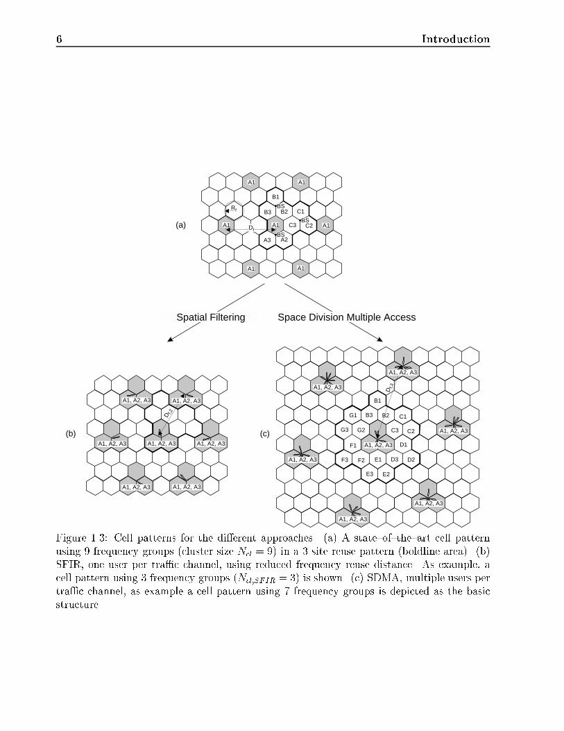
to Ncl;SFIR = 3, which increases system capacity by a factor of three. Figure 1.2c showsan SDMA system having a cluster size Ncl;SDMA = 9 with three users (in the mean) perfrequency and timeslot. This also leads to a capacity increase of a factor three. Bear in mindthat these values for capacity increase are just examples and do not necessarily represent thereality. Realistic values can be found in Chapter 9.
Mobile communications systems are already partially making use of the directional dis-tribution of the incident signals at the BS by using sector antennas. If such a system isupgraded by SFIR or SDMA the cell layout philosophy changes. Figure 1.3a shows a conven-tional system using a 3/9 cell pattern. The BSs are located in the center of three cells, whichsaves infrastructure costs. If this system is upgraded with SFIR or SDMA, the three neigh-bouring sectors are combined to one cell, e.g. the frequency groups A1, A2, and A3 in the 3/9conventional cell pattern can now be used all together in one cell. The "cell", i.e. the part ofthe cellular network, where one dedicated group of frequencies is used, is larger as comparedto the sector cell. Figure 1.2b shows an SFIR{system having a cluster size of Ncl;SFIR = 3,whereas Figure 1.2c shows an SDMA system having a cluster size of Ncl;SDMA = 9. Bothsystems evolved from a sector cell layout of the original system. This �gure shows that weare again going back to a system providing "omnidirectional" coverage. This will increasetrunking e�ciency, since the available trunk pool at one BTS has in my example three timesmore channels than the corresponding trunk pool of the sectorized system at the same BTS.
Assume a blocking rate of 1% and a subscriber usage of 0.03 Erlangs [Lop96]. Theconventional cellular system may have 15 channels assigned to one 120�{sector of a cell(trunking group). Using the formula for the number of subscribers per channel of [Lop96], Iget for the number of subscribers per channel, NS=CH = 18:6. If we use SFIR we are able tocombine the trunking groups of the three sectors to one trunking group having 45 channels.The number of subscribers of one channel of the SFIR system follows as NS=CH=SFIR = 24:3,which is an increase of 31% as compared to the conventional system layout.
Reference [Tan94] claimed an increase in spectrum e�ciency with SFIR bypM , where
M denotes the number of antenna elements. For SDMA a capacity increase bypMK, where
K is the number of beams on the same frequency and timeslot, is achievable [Tan94]. Thenumber of beams is the number of users served simultaneously at the same frequency andtimeslot. Applying these formulas for M = 8 antenna elements, SFIR would give an increasein spectral e�ciency of
pM = 2:8 and SDMA with K = 3 would give
pMK = 4:9. These
are impressing values, but bear in mind that they are obtained by assuming ideal conditions:The positions of the users (incidence angles of the signals) are determined exactly, there areno array imperfections, and the assumed antenna hardware is perfectly linear.
The RACE II TSUNAMI (Research and development in Advanced Communications inEurope II | Technology in Smart Antennas for UNiversal Mobile Infrastructure) projectperformed research into smart antennas for next generation mobile communications systems.They proposed a broadband receiver structure allowing multiple carriers and beams from/toeach antenna element. They identi�ed three key areas for a system deploying smart antennas:
1. Baseband DSP (Digital Signal Processing): Beamforming for both up{ and down-link is accomplished at baseband (DB, Digital Beamforming), the shaped signals areafterwards upconverted to passband. This gives exibility, robustness, and performanceenhancement, since sophisticated algorithms can be utilized. Due to technology con-straints in DSP the time span for the project was too short to implement and compare
6 Introduction
A1A1
A1 A1
A1 A1
A1
A2A3
C1
C2C3
B1
B2B3BS
BS
BS
Spatial Filtering Space Division Multiple Access
Rf
(a)
(b) (c)
Df
D f,2
A1, A2, A3 A1, A2, A3
A1, A2, A3 A1, A2, A3
A1, A2, A3
A1, A2, A3 A1, A2, A3
C1
C2C3
B1
D1
E1
F1
G1 B2
D2
E2
F2
G2
B3
D3
E3
F3
G3
Df,3
A1, A2, A3
A1, A2, A3
A1, A2, A3
A1, A2, A3
A1, A2, A3
A1, A2, A3
A1, A2, A3
Figure 1.3: Cell patterns for the di�erent approaches. (a) A state{of{the{art cell patternusing 9 frequency groups (cluster size Ncl = 9) in a 3 site reuse pattern (boldline area). (b)SFIR, one user per tra�c channel, using reduced frequency reuse distance. As example, acell pattern using 3 frequency groups (Ncl;SFIR = 3) is shown. (c) SDMA, multiple users pertra�c channel, as example a cell pattern using 7 frequency groups is depicted as the basicstructure.

1.3 Change in System Architecture 7
di�erent algorithmic and structural approaches [Bul95]. Furthermore, the performanceof the algorithms increases continuously with the many groups investigating smart an-tennas. While there is a vast number of proposed algorithms for this application, theabsence of published comparisons of these techniques hinders practical engineering ef-forts such as cellular system design. Therefore this topic is addressed in more detail inthis thesis.
2. Antenna Elements: The antenna elements developed for TSUNAMI are microstrippatch antennas. A multilayer structure with a ring and a parasitic patch was selected,since it is capable of wideband operation (220 MHz at 2 GHz), while giving a gain ofmore than 6dBi [Gar95].
Aperture{coupled microstrip patch antennas developed at our department, however,outperform these structures in bandwidth considerably [Kuc96a], [Kuc96b].
3. Linear RF Hardware: Special e�ort was placed to build RF{antenna frontends withhighly linear ampli�ers. This is necessary, since beamforming is done with digital cir-cuit technology at baseband. This poses high linearity demands on both the RF/IF(Intermediate Frequency) up{ and downconversion chain. Because the weights of thebeamformer are determined at digital baseband, any distortion in the up{ and down-conversion chain alters the antenna pattern [Xue95]. While �xed mismatches betweenthe di�erent channels can be calibrated, the non{linear e�ects in the transceiver chaincause intermodulation which cannot be compensated in any practical way.
Other key parts of smart antenna systems identi�ed at our department are (1) the syn-chronism between the I{ (Inphase) and Q{ (Quadrature) branch of the receiver and (2)calibration of the system. The �rst item can be solved by IF{sampling in conjunction withDDC (Digital Down Conversion) [Kon96]. Sophisticated calibration is necessary since allalgorithms applied at baseband rely on an ideal model of the receiver. Since in real{worldreceivers a couple of impairing e�ects are present, they have to be eliminated in a preprocess-ing step. This necessitates both the incorporation of hardware components and calibrationalgorithms [Kon95], [McC94], [Ali93].
Smart antennas are applicable to both the BS and the MS of a cellular mobile communi-cations system. As I will show in the next chapters, such antennas have typically in the orderof ten elements spaced by a half wavelength. For the frequency ranges of today's and nextgeneration's cellular mobile communications systems a smart antenna system is (a) possiblytoo large to be implemented at mobile and portable units, and (b) the power consumptionof the whole signal processing chain has to be taken into due consideration for these units.Therefore I consider the application of smart antennas on the BS only.
1.3 Change in System Architecture
Smart antennas a�ect four parts of mobile communications systems architecture:
� BS Antenna: Up to now typical BS antennas are vertical linear arrays to concentratethe energy in elevation, in azimuthal direction they have omnidirectional or sectorpatterns [Kat92]. A �xed feeding circuit in hardware is usually implemented directly at

8 Introduction
the antenna, therefore only one cable connects the antenna with the transceiver. Thenew technology, however, requires an adaptive array, where the signals of the di�erentantenna elements are processed separately and combined afterwards in order to extractthe desired information. Since we now want to concentrate the energy primarily inazimuth, horizontal linear array structures are necessary. Measurements have shownthat for outdoor environments the horizontal angular spread is typically much largerthan the vertical spread [Egg95a], [Kle96b], therefore processing of the outputs of ahorizontal linear array is considered to be su�cient. Antenna elements in verticaldirection can also be added, however, just to increase directivity of the antenna (pseudo{planar array). Figure 1.4 shows this change in BS antenna technology. Figure 1.4a1depicts the conventional architecture of a BS with three downtilted sector antennas tocover an entire 360� cell. Figure 1.4b1 shows the according con�guration of a smartantenna system. Figures 1.4a2 and 1.4b2 show the antenna patterns both for aconventional BS antenna system and the smart antenna solution. The advantages ofthe more narrow beam for smart antennas and their ability to track the user and toput nulls onto interfering signals (users) leads to increased system performance.
� BS Receiver (Transmitter): The change in system requirements also a�ects re-ceiver and transmitter structures. In Figure 1.5a a state{of{the{art receiver structureis shown. Figure 1.5b depicts the architecture and the receiver structure for a systemutilizing smart antennas. For the new system the signal of each antenna element hasto be downconverted to baseband, A/D (Analog/Digital) converted, and processed bya signal processing unit.
The same remarks hold for the transmitter.
� Signal Processing: Powerful array signal processing algorithms in conjunction withsophisticated channel allocation strategies have to be utilized at the BS. Channel allo-cation, handover algorithms and procedures become more complex. In order to keepthe data transfered between the BTS and the BSC (Base Station Controller) in a rea-sonable size, the BTSs have to be equipped with more "intelligence". This is especiallynecessary for 2nd generation systems (GSM, DCS1800).
� Protocols: For smart antennas to be introduced into 2nd generation mobile commu-nication systems with already speci�ed protocols one has to adjust the smart antennasystem to �t into the given frame. Of course, this would not always lead to the opti-mum solution. Large changes in the protocols to enable the utilization of smart antennasystems are not to be expected. This motivates us to �nd solutions that �t into theexisting standards. The most critical areas are identi�ed to be the initial log{in of theterminal, the handover procedures, and the radio resource management [Rhe95]. Incontrast, protocols for next generation mobile communications systems should incor-porate requirements for smart antennas to ease their application and to get optimumperformance at the smallest possible cost.
The �rst commercial products appear right now [NoT95], [Nah96]. However, they rely onrather simple techniques which must be improved considerably to reach the desired goals ofsmart antenna processing.

1.3 Change in System Architecture 9
StackedAntenna
Structures
1
2
3
Ns
-30
-20
-10
0Sector 1 Sector 1
Sect
or 2
Sect
or 2
Sector 3
Sector 3
Gai
n (d
B)
User 1
(a1)
(a2) (b2)
(b1)
User 1
User 2 User 2User 3 User 3
Gai
n (d
B)
-30
-20
-10
0
Figure 1.4: BS antenna con�gurations. (a1) Conventional 3 � 120� sector antennas, (b1)Smart antenna, (a2) Antenna patterns, (b2) Antenna patterns of the smart antenna.

10 Introduction
Phy
sica
l Ant
enna
Phy
sica
l Ant
enna
Fix
ed C
ombi
ning
Net
wor
k
Downconversion& Filtering
Downconversion& Filtering
Downconversion& Filtering
Downconversion& Filtering
Downconversion& Filtering
Sampling Processor& A/D (RAM)
Sampling Processor& A/D (RAM)
(a)
(b)
Sampling Processor& A/D (RAM)
Sampling Processor& A/D (RAM)
Sampling Processor& A/D (RAM)
Digital SignalProcessing
Sm
art A
nten
naS
igna
l Pro
cess
ing
Uni
t(B
eam
form
ing,
Use
r S
epar
atio
n, ..
.)
Data UserK
Data User2
Data User1
Data User1
I
I
I
I
Q
Q
Q
Q
Figure 1.5: Receiver structures for BTS of mobile communications systems. (a) State{of{the{art receiver, (b) Receiver structure for a system utilizing smart antennas.

Chapter 2
Channel Modeling Including DOAs
Channel modeling is an important issue for mobile communications systems performanceassessment. Given a description of the channel, e�cient processing schemes may be devisedand system performance can be analyzed. To study smart antenna schemes, a channel modelincluding DOAs has to be utilized. The PDPs (Power Delay Pro�les) speci�ed by COST207 [Cos89] (European Cooperation in the Field Of Scienti�c and Technical Research) arenot directly applicable, since no DOAs are speci�ed. It is impossible to derive DOAs fromthe Doppler pro�les for these PDPs since the positions of the scatterers and the position,the velocity, and the moving direction of the mobile are unknown. At the mobile, signalsusually are incident from all directions, giving rise to the classical Doppler pro�le. At the basestation, however, the DOAs are con�ned to certain areas as the measurements of [Egg95a],[Kle96b], and [Mar96a] clearly indicate.
The �rst channel model including a directional component, i.e. DOAs and an angular dis-tribution of the incoming signals was proposed by Lee in 1974 [Lee73]. This model, however,was primarily intended for determination of the correlation of signals received at di�erentantennas to predict the performance of diversity schemes. Later, this model appeared asstarting point for smart antenna investigations [And91], [Win93], [Zet95a]. It was named thelocal scatterer model.
Ref. [Bla95] introduced a propagation model, where the scatterers are located in circularregions around the MS and for micro{ and picocell scenarios also around the BS. This modelis a useful starting point, however, the number of scatterers proposed for that model shouldbe reduced considerably in order to cut down the computational complexity.
A di�erent model was introduced by [N�r94]. It assumes that the scatterers are placed atellipses with the BS and the MS in their foci. The dimensions of the ellipse are determined bythe actual propagation delay. The path loss exponent between the MS and the scatterers andbetween the scatterers and the BS can be di�erent in order to match di�erent propagationconditions. This is necessary, since the BS may not have LOS (Line Of Sight) to the somescatterers, whereas the MS may have LOS to these scatterers.
A geometrically based model for LOS multipath radio channels was proposed in [Lib96b].It provides a structure in which short delay multipath components are more likely to arrivewith DOAs near the direct path, while multipath components with longer delays are moreuniformly distributed in their DOA.
Measurements determining the DOAs and angular spreads in rural areas, micro{, andpicocells have been performed by [Egg94]. They support the local scatterer model for rural
11

12 Channel Modeling Including DOAs
environments and the geometrically based model for LOS multipath channels for micro{and picocells. The measurements conducted by [Kle96b] for rural, suburban, and urbanenvironments with BS antennas above the rooftops and the measurements of [Mar96a] inurban areas all support the local scatterer model.
This chapter gives an introduction into channel modeling including DOAs, discusses therelevant de�nitions, introduces high{rank and low{rank models, and analyzes the local scat-terer model in detail.
2.1 Basic Modeling
Assume an antenna array with M elements which serves K users simultaneously. The fun-damental description of the linear multipath medium between the users and the antenna isgiven by the impulse response matrix
H(�; t) =
266666664
h11(�; t) h12(�; t) : : : h1m(�; t) : : : h1M (�; t)h21(�; t) h22(�; t) : : : h2m(�; t) : : : h2M (�; t)
......
. . ....
. . ....
hk1(�; t) hk2(�; t) : : : hkm(�; t) : : : hkM(�; t)...
.... . .
.... . .
...hK1(�; t) hK2(�; t) : : : hKm(�; t) : : : hKM(�; t)
377777775; (2.1)
where hkm(�; t) denotes the instantaneous complex impulse response for transmission fromthe k{th user to the m{th antenna element. � denotes the delay time and t is the absolutetime. The instantaneous complex impulse response from the k{th user to the m{th antennaelement is given by
hkm(�; t) =
LtXl=1
gl;km(t)�(� � �l); (2.2)
where Lt is the number of distinct paths in the temporal domain, gl;km(t) is the amplitudeof the l{th path, and �(:) denotes Dirac's delta pulse. This is a usual channel model used forperformance assessment of mobile communication systems. For notational convenience I willneglect the index (:)km in the sequel to facilitate readability.
The directional component of the impulse response is incorporated in gl(t) via the relation
gl(t) =
2�Z'=0
�Z�=0
~gl;MS(t; '; �) sin(�) d� d'
=
2�Z'=0
�Z�=0
~gl;BS(t; '; �) sin(�) d� d'; (2.3)
where ~gl;MS(t; '; �) (~gl;BS(t; '; �)) is the instantaneous directional distribution of the channelimpulse response at the time instant t (incorporating all components with a delay of �l) at theMS (BS), ' denotes the azimuthal angle, and � denotes the polar angle, which is measured

2.1 Basic Modeling 13
from the z{axis. The elevation angle # follows as # = �=2 � �. In the sequel, I will usethe term ~gl(t; '; �) to denote a directional distribution of the channel impulse response at anarbitrary location (BS or MS).
The instantaneous directional distribution of the channel impulse response at the MS,~gl;MS(t; '; �) is in general di�erent from the instantaneous directional distribution of thechannel impulse response at the BS, ~gl;BS(t; '; �), whereas the strength of the l{th path gl(t)is independent of the location. This e�ect is addressed in a more general way in Section2.2. At the �rst glance this may sound like a contradiction of the reciprocity theorem. It isde�nitely not a contradiction, the di�erence is caused by the di�erent environments of theBS and the MS, and, consequently, their "view" of the situation.
Inserting Equation (2.3) into Equation (2.2) and interchanging the summation and theintegration yields
h(�; t) =
2�Z'=0
�Z�=0
hMS(�; t; '; �) sin(�) d� d'
=
2�Z'=0
�Z�=0
hBS(�; t; '; �) sin(�) d� d'; (2.4)
where
hMS(�; t; '; �) =LtXl=1
~gl;MS(t; '; �)�(� � �l) (2.5)
is the instantaneous directional impulse response at the MS and
hBS(�; t; '; �) =LtXl=1
~gl;BS(t; '; �)�(� � �l) (2.6)
is the instantaneous directional impulse response at the BS.
Consider the plane scenario (� = �=2) depicted in Figure 2.1. For the delay �l one scattererlies on the corresponding ellipse with the BS and the MS in its foci. The contribution of thisscatterer to the instantaneous directional distribution of the channel impulse response at theBS is
~gl;BS(�; ') = (2.7)
(r(M)l r(l)m )��=2ale
j�l�(t� r(M)l + r
(l)m
c0)�('� 'l;BS)e
�j 2��vM cos('l;BS�'vMS
)tej2�(r
(M)l
+r(l)m )
� ;
and at the MS
~gl;MS(�; ') = (2.8)
(r(M)l r(l)m )��=2alej�l�(t� r
(M)l + r
(l)m
c0)�('� 'l;MS)e
�j 2��vM cos('l;BS�'vMS
)tej2�(r
(M)l
+r(l)m )
� ;

14 Channel Modeling Including DOAs
vM
BS
MS
Scattering point lA
nten
na e
lem
ents
ϕl,BS
ϕl,MS
ϕvMS
12
M
r(l)mr(M)
l
m
Figure 2.1: Propagation scenario where the l{th of the Lt paths linking the m{th antennaelement of the base station, BS, and the mobile station, MS, is high{lighted.
where r(M)l and r
(l)m denote the distance from the mobile to the l{th scatterer and the distance
from the l{th scatterer to the m{th antenna element of the BS, respectively. For the BS (MS)the l{th scattering point appears under the azimuth angle 'l;BS ('l;MS) and is characterizedby a scattering coe�cient ale
j�l. The angle 'l;BS depends also on the location of the m{thantenna element. Since I assume that the scattering points are in the far �eld of the BSantenna, this dependence is neglected. The mobile is assumed to have velocity ~vMS so thatr(M)l varies with the absolute time t. 'vMS
is the azimuthal angle of the velocity vector ~vMS.� denotes the power attenuation exponent, f0 is the carrier frequency and c0 is the velocityof light. The operator is de�ned by
r(M)l r(l)m =
(r(M)l r
(l)m : for scattering
r(M)l + r
(l)m : for specular re ections
: (2.9)
In general, many scatterers contribute to the impulse response. Furthermore, multiple scat-tering has to be incorporated when determining the impulse response.
The detailed analysis of channel models is based on precise de�nitions for the character-istics of the mobile radio channel. These de�nitions can be found in Appendix A.
2.2 Low{Rank and High{Rank Channel Models
The received signal power in mobile communications experiences uctuations that can bedivided into (Figure 2.2)
� Large{Scale Fading: If the receiver moves through a scattering scenario, new scat-terers appear and other scatterers disappear. Additionally the morphology of the en-vironment (shadowing) a�ects the received signal power. The received signal variesrather slowly (depending on the movement speed of the mobile), this e�ect is calledlarge{scale fading. The terms slow fading and long{term fading are also sometimes usedto describe this process.
� Small{Scale Fading: Additionally to the large scale fading there are also signi�cantsignal variations if the receiver moves a few wavelengths or even only fractions of a

2.2 Low{Rank and High{Rank Channel Models 15
Sig
nal p
ower
Time t
Large scale fading
Small scale fading
Figure 2.2: Large scale and small scale fading in mobile communications.
wavelength. These are caused by interference of signals from scatterers around thereceiver. The distance between two fading dips is in the order of �=2, where � denotesthe wavelength. This e�ect is called small{scale fading. The terms fast fading andshort{term fading are also sometimes used to describe this phenomenon.
If the transfer function of the mobile radio channel is observed in the frequency band ofinterest, two di�erent kinds may appear:
� Flat Fading: The transfer function is constant over the frequency range of interest,but varies with time t. This is called a nondispersivly fading or a at{fading channel.It occurs if the delay spread St of the channel is small compared to the inverse of thereceiver �lter bandwidth Bfilter,
St � 1
Bfilter: (2.10)
� Frequency{Selective Fading: The transfer function varies over the band of interestand is a function of time t. This is called a time{dispersive or frequency{selectivechannel. It occurs if the delay spread St is equal to or larger than the inverse of thereceiver �lter bandwidth Bfilter,
St &1
Bfilter: (2.11)
These descriptions do not include the angular domain. To include this new dimension,Reference [Ott96] distinguishes between two di�erent types of channel models
1. Low{rank channel models
2. High{rank channel models

16 Channel Modeling Including DOAs
Flat fading
Frequency-selective fading
Low rank
High rank
S<<1/Bfilter
S>1/Bfilter S>1/Bfilter
S<<1/Bfilter
Sϑ,ϕ<ϑ3dB,ϕ3dB
Sϑ,ϕ>ϑ3dB,ϕ3dB
and
and/or
Figure 2.3: The relations between at fading, frequency{selective fading, low{rank, and highrank channels. The latter are a generalized version of the former.
Due to the absence of a clear de�nition in [Ott96] I will give one in the sequel.
Let '3dB(�3dB) denote the 3dB{beamwidth of the antenna array at the BS in azimuth(elevation) with equal{amplitude and equal{phase feed currents | which is the minimum3dB{beamwidth [Stu81].
De�nition: A channel is low{rank if the delay spread St is small compared to the inverseof the receiver �lter bandwidth Bfilter and the angular spread (S'; S�) is small compared tothe 3dB{beamwidths ('3dB; �3dB) of the antenna pattern (as de�ned above),
St � 1
Bfilter; S' � '3dB; and S� � �3dB: (2.12)
A channel is high{rank if the delay spread St is equal to or larger than the inverse of thereceiver �lter bandwidth Bfilter or the angular spread (S'; S�) is equal to or larger than the3dB{beamwidths ('3dB; �3dB) of the antenna pattern,
St &1
Bfilter; or S' & '3dB; or S� & �3dB: (2.13)
Figure 2.3 shows a graph with the relations between these channel types. One intuitiveexplanation of the di�erence between high{rank and low{rank channels is as follows: Assumethat one MS communicates with its associated BS. The output signal vector of the BS antennaarray is given by
x(�; t) =
266666664
x1(�; t)x2(�; t)
...xm(�; t)
...xM (�; t)
377777775=H(�; t)s(�) + n(�); (2.14)

2.3 Low{Rank Channel Models 17
where n(�) is the ST{AWGN (Spatio Temporal Additive White Gaussian Noise) vector(see Chapter 3) and
s(�) =
26664
s(�)s(� � T )
...s(� � (Lchannel � 1)T )
37775 (2.15)
is the vector containing the transmitted signals from the mobile, where Lchannel denotes thelength of the channel impulse response normalized to a symbol duration T . If the channelis low{rank, then Lchannel = 1, i.e. s(�) degenerates to a single (complex) number. Thiscondition, however, is only necessary but not su�cient, since the angular spread may belarger than the 3dB{beamwidth of the array.
Another intuitive explanation is that a channel is high{rank whenever some kind of di-versity | time diversity by applying an equalizer, or angle (pattern) diversity by applying asmart antenna | can be utilized to increase system performance.
2.3 Low{Rank Channel Models
The most prominent low{rank channel model is the local scatterer model. It accounts forthe directional component of the mobile radio channel. This is achieved by modeling thescattering situations by a spatial distribution function. For instance, in rural and suburbanmobile radio the BS antenna, which is usually above the rooftops, has typically LOS to thevicinity of the mobile. The local scattering around the mobile generates signals that arrivemainly within a given range of angles at the BS antenna. Figure 2.4 shows a typical scenario,where the signals from the mobile arrive at the BS within �� at an angle '0. Note that ifthe MS is near the BS, the local scatterer model may also be a high{rank model, since theangular spread might be larger than the 3dB beamwidth of the antenna pattern.
The local scatterer model was analyzed in Refs. [Lee73], [Ada86], and [Sal94], wheretheoretical and experimental results showed the relationship of DOA and beamwidth withthe correlation of the fading between di�erent antennas.
2.3.0.1 Spatial Distribution Functions of the Scatterers
To incorporate a spatial component into the channel model a PDF (Probability DensityFunction) for the DOAs of the waves is applied.
References [Egg95a], [Lee73], and [Ott96] showed by measurements and theoretical anal-ysis that the DOAs for a BS antenna above the rooftop in rural and suburban mobile radioare not discrete. Rather they consist of a nominal DOA associated with an angular spread.
The spatial distribution function p1(r) of the scatterers around the mobile station can bemodeled as
p1(r) =
�1
R2�: kr � rMSk � R
0 : elsewhere; (2.16)

18 Channel Modeling Including DOAs
BS
MSScatterers
Antenna Elements1 2 Mm
ϕ0∆ ∆
Figure 2.4: Propagation scenario, where all signals from a mobile arrive at the base stationwithin �� at an angle '0.
where r is the radial distance measured from the MS's position, R is the radius of the scatterercircle, and rMS is the distance between BS and MS. According to [Lee94], R is typically inthe order of 100�200�1, independent of the distance between BS and MS. However, relevantscatterers are more likely to be near the MS than far away, and not to have a sharp drop asin the model above. Therefore I use
p2(r) =1
2�R2e�
(r�rMS)2
2R2 ; (2.17)
which is a Gaussian distribution function. Figure 2.5 shows these PDFs for a radius of thescatterer circle R = 200�. At the position of the MS, the PDF of the scatterers pi(r); i = 1; 2is identical to the directional distribution of the absolute value of the channel impulse responseat the MS p(k~gl;MS(t; '; �)k), for all � , if the local mean values of the scatterer coe�cientsare equal and the di�erences in the propagation loss of the di�erent paths are neglected.
I will now derive an analytical formula for the directional distribution of the absolutevalue of the channel impulse response at the BS. This can be done only for the GaussianPDF of Equation (2.17). Let the BS and the MS be in the foci of an ellipse, and assume theBS to be in the origin of the coordinate system. The parameters of the ellipse are then givenby (Figure 2.6) [Bar86]
2e = rMS = �minc0; (2.18)
2a = �c0; (2.19)
and
b =pa2 � e2 =
c02
q� 2 � � 2min: (2.20)
1In rural and suburban macrocell scenarios the radius R might be independent of the wavelength andmuch larger than the values given here. Detailed measurements to determine the possible range for R arenecessary.

2.3 Low{Rank Channel Models 19
−500
0
500
−500
0
5000
1
2
3x 10
−4
6
p1(r)
QQQQk
y � yMS=���
���1
x� xMS=� −500
0
500
−500
0
5000
1
2
3x 10
−4
6
p2(r)
QQQQk
y � yMS=������1
x� xMS=�
Figure 2.5: Probability density functions for the spatial distribution of the scatterers aroundthe mobile station. xMS = 0 and yMS = 0 denote the position of the MS.
MS
ϕr(ϕ)2a-r(ϕ)
erMS=2e
e x
y
b
BS
Figure 2.6: The characteristic dimensions of an ellipse.
The distance from the BS to the scattering point lying in direction ' at a time instant�1 � �min follows therefore as
r(') =b2
a+ e cos('): (2.21)
The distance of the scattering point to the MS is therefore
r(M)l (') = 2a� r(') = 2a� b2
a + e cos('): (2.22)
Inserting this into Equation (2.17) gives
p(k~gl;BS(t; '; �)k) =1
2�R2e�
(r(M)l
('))2
2R2 =
=1
2�R2e�
c0(�
2+2��min cos(')+�2min)
2(�+�min cos('))
!2
2R2 ; (2.23)
which is the directional distribution of the absolute value of the channel impulse response atthe BS.

20 Channel Modeling Including DOAs
Figure 2.7 shows the directional distribution of the absolute value of the channel impulseresponse for the BS and the MS for the two PDFs of Equations (2.16) and (2.17) withR = 200� and rMS = 1200�. The di�erence between the BS and the MS is striking. It is dueto the local scatterers, which are far from the BS around the MS. The PDF of the directionaldistribution of the absolute value of the channel impulse response at the BS for some �xeddelays � = �l is shown in Figure 2.8. It shows the spread{out DOA for the correspondingdelay instant. The integration over all possible delays leads to a PDF of the azimuthalangular distribution. It is shown in Figure 2.9. Dependent on the spatial distribution of thescatterers di�erent PDFs for the azimuthal angular distributions are proposed in literature.
Reference [Lee73] proposed
p';1('l) =
�Q1
�cosn('l � ') : ��=2 + ' � 'l � �=2 + '
0 : elsewhere; (2.24)
where n is an even integer and Q1 is a normalizing constant chosen to make p('; i) a PDF,i.e.
�=2+'Z��=2+'
p('l) d'l = 1: (2.25)
Reference [Sal94] used
p';2('l) =
�12�
: ��+ ' � 'l � �+ '0 : elsewhere
; (2.26)
mainly for deriving a closed form expression for the envelope correlation coe�cient �envbetween the received signals at di�erent antenna positions. Figure 2.9 shows that the as-sumption of a uniform PDF for the arrival angles is even not valid for the uniform scattererdistribution.
References [Ada86], [Tru96] proposed
p';3('l) =Q3q2��2�
e� ('l�')2
2�2� ; for � �=2 + ' � 'l � �=2 + '; (2.27)
where �� is the standard deviation of the spread{out DOAs in the angular domain and Q3
is a normalization constant in order to make p';3('l) a PDF. The three functions are shownin Figure 2.10 for an angular spread of S' = 5�. I determined the angular spread as
S' =
8<:
�=p3 : uniform PDF
��
rQ3erf
��p8��
�: Gaussian PDF
(2.28)
where erf(a) is the real{valued error function given by
erf(a) =2p�
aZx=0
e�x2
dx: (2.29)

2.3 Low{Rank Channel Models 21
0.50
0.5
0.5
0
0.50
1
2
3x 10
-4
0.50
0.5
0.5
0
0.50
1
2
3x 10
-4
0.50
0.5
0.5
0
0.50
1
2
3x 10
-4
0.50
0.5
0.5
0
0.50
1
2
3x 10
-4τ/
µs τ/µs
τ/µs
τ/µs
µs
µs µs
µs µs
µsµs
µs
(a) (b)
ϕ
ϕϕ
ϕ
p( gl,MS(t,ϕ,θ) )
p( gl,MS(t,ϕ,θ) )
p( gl,MS(t,ϕ,θ) )
p( gl,MS(t,ϕ,θ) )
Figure 2.7: Directional distribution of the absolute value of the channel impulse response forthe BS and the MS for (a) the uniform PDF, (b) the Gaussian PDF of the location of thescatterers around the MS.

22 Channel Modeling Including DOAs
140 160 180 200 2200
0.5
1
1.5
2
2.5
3x 10⁻⁴
6
p(kgl;BS(t; '; �)k)
-' (deg)
���
� = �min
���� = 1:2�min
��
� = 1:4�min� = 1:6�min
140 160 180 200 2200
0.5
1
1.5
2
2.5
3x 10⁻⁴
6
p(kgl;BS(t; '; �)k)
-' (deg)
����� = �min
��� = 1:2�min
��� = 1:4�min
��
� = 1:6�min
(a) (b)
Figure 2.8: Probability density functions of the directional distribution of the absolute valueof the channel impulse response at the BS for some �xed delays � = �l . (a) uniform PDF ofthe scatterers around the MS, (b) Gaussian PDF of the scatterers around the MS.
140 160 180 200 2200
1
2
3
4
5
6
7
86p'(')
-' (deg)
���Gaussian PDF�
���
Uniform PDF
Figure 2.9: PDF of the azimuthal angular distribution of the incident waves for the scenariosconsidered in Figures 2.8 and 2.7.

2.3 Low{Rank Channel Models 23
−20 −10 0 10 200
1
2
3
4
5
66p';i(')
-' (deg)
���Uniform PDF
���Gaussian PDF
@@@
Cosine PDF
Figure 2.10: Di�erent probability density functions for an angular spread of S' = 5�. Thecurve for the Gaussian PDF is shifted by "1" in the ordinate, since otherwise it would bemasked by the cosine{shaped PDF.
The curve for the Gaussian PDF is shifted by "1" in the ordinate, since otherwise it wouldbe masked by the cosine{shaped PDF. This graph shows that the cosine{shaped PDF isessentially the same as the Gaussian PDF. In the sequel I therefore consider only the uniformPDF and the Gaussian PDF.
These PDFs rely on the assumption that there is no local scattering around the BS. Iflocal scattering around the BS has to be taken into account, as e.g. for antennas near orbeyond rooftop level, a uniform distribution function
V (') =1
�2
with �2 � 1
�for � �=2 + ' � 'l � �=2 + '; (2.30)
is added to the PDFs
~p';i('l) =1
�s
(p';i('l) + V (')); 1 � i � 3; (2.31)
where the constant �s is chosen in order to make ~p';i('l) a distribution function, i.e.
�=2+'Z��=2+'
~p';i('l) d'l = 1: (2.32)
2.3.1 Angular Spread
At the BS the incoming signals of the MS have an angular spread dependent on the distancebetween BS and MS, rMS, and the radius of the scattering circle, R. Measurements of [Egg96]and [Lee73] have shown that R is independent of the distance between BS and MS, rMS, as

24 Channel Modeling Including DOAs
long as we have NLOS (Non|LOS). I am now interested in the distribution function of theangular spreads the BS "sees".
Suppose the MS's as uniformly, but randomly distributed within a circular area with outerradius r2 and inner radius r1. The area of this ring is given by
A = �(r22 � r21): (2.33)
The CDF (Cumulative Distribution Function) F (rMS � ri) of the radius rMS of the locationof the mobile to be less than ri is calculated as
F (rMS � ri) =
'=2�Z'=0
rMS=riZrMS=r1
1
ArMS drMS d' =
r2i � r21r22 � r21
: (2.34)
From this result the PDF p(rMS) of rMS is found as
p(rMS) =dF (rMS = ri)
drMS=
� 2rMS
r22�r21: r1 � rMS � r2
0 : elsewhere: (2.35)
The angle under which the radius of the scattering circle is seen at the BS is
� = arctan
�R
rMS
�: (2.36)
The PDF p(�) of the angle � can be found by the variable transform
p(�) = p(rMS)
����drMS
d�
���� ; (2.37)
with
drMS
d�=
�Rcos2(�) tan2(�)
(2.38)
as
p(�) =R2
cos2(�) tan3(�)(r22 � r21): (2.39)
With �0 as the minimum angle
�0 = arctan
�R
r2
�(2.40)
the CDF F (�) is found as
F (�) =
�=�Z�=�0
p(�) d� =R2
(r22 � r21)
�1
sin2(�0)� 1
sin2(�)
�: (2.41)
The CDF of the angular spread can be found by simply transforming the angle � into theassociated angular spread via the relations (2.28). Figure 2.11 gives the CDF of the angularspread when the scatterers are uniformly distributed around the MS with the outer cell radiusr2 as parameter. For an outer cell radius of 10000�, which is 1600m for a wavelength of 16cm (DCS 1800), 90 % of the angular spreads are less than 2:2�. In typical macrocells (radiir2 > 1km), small angular spreads dominate.

2.3 Low{Rank Channel Models 25
0 5 10 15 20 250
0.2
0.4
0.6
0.8
16F (S')
-S' (deg)
@@@
r2 = 1000�
@@@
r2 = 20000�
@@@
r2 = 10000�
@@@
r2 = 5000�
Figure 2.11: Cumulative distribution function of the angular spread, when the scatterers areuniformly distributed around the MS. The radius of the scattering circle is R = 400�, theinner cell radius r1 = 200�, and the outer cell radius r2 as parameter. {: r2 = 20000�, ��:r2 = 10000�, �:�: r2 = 5000�, and : : : :: r2 = 1000�.
2.3.2 Fading Correlation
For an analytical expression of the fading correlation at di�erent receive positions, I startwith the scenario depicted in Figure 2.4. The derivation follows closely Reference [Sal94].Assume that a narrowband signal s(�)ej!0� , where !0 = 2�f0 is the radian center frequency,is sent while the mobile is moving through the scattering area. This signal is received by anarbitrarily orientated equispaced array of antennas with spacing d. I consider NLOS propaga-tion only, therefore all received waves stem from scatterers surrounding the MS. Furthermore,I assume that the statistical properties of the scattering channels remain unchanged whilethe mobile is moving (stationarity), therefore I omit the absolute time t in the equations.The distance between the BS and the MS is assumed to be much greater than the Rayleighdistance of the antenna array and the distance from the mobile to the scatterers. We arein the far �eld of the transmit antenna and can assume the incident waves as parallel. Thereceived signal at the m{th antenna is
sr;m(�) =LtXl=1
gl;1ms(� � �l)ej!0� : (2.42)
Suppose that the reference sensor of the array is sensor #1. I assume the amplitude of thel{th path from the MS to the reference sensor of the BS to be
gl;1m =
NlXnl=1
�gnl;1m; (2.43)

26 Channel Modeling Including DOAs
i.e. it is the sum of a large number of terms. Then, the nl{th signal arriving at element msu�ers a delay
� (m)nl
= (m� 1)d
c0sin('nl); k'nlk � �; (2.44)
where 'nl is the DOA of the nl{th path centered around the nominal DOA '0. For narrow-band signals this delay can be modeled as a phase shift
�(m)nl
=2�
�(m� 1)d sin('nl): (2.45)
Since
�lm = (m� 1)d sin('nl)� r(l)m ; (2.46)
i.e. the di�erence of the path length between the scatterer and the �rst antenna element andthe scatterer and the m{th antenna element is negligible compared to the distance betweenthe antenna elements and the scatterer, I can write for the amplitude of the l{th path
kgl;11(t)k = kgl;12(t)k = kgl;1m(t)k = kgl;1M(t)k = kgl(t)k; 8t: (2.47)
The quantity gl;1m is therefore given by
gl;1m =
NlXnl=1
�gnlej( 2�
�(m�1)d sin('nl )+!0�nl ); (2.48)
The terms �gnl are random complex quantities. Furthermore, I assume that there are a largenumber of terms in each sum (Nl ! 1). Consequently, from the central limit theorem, thegl's are independent, complex, zero mean, Gaussian random variables.
The envelope of the received signal at each delay instant �l, ksrm(�l)k, is the sum of twoGaussian distributed random variables, each of the form Refsrm(�l)g � N (0; �) (Imfsrm(�l)g �N (0; �)), and is therefore Rayleigh distributed, i.e. ksrm(�l)k � RA(p�
2�;p2�). Both the
real part and the imaginary part of the received signal have the same statistical properties.
The abbreviation s � X (m; �) stands for: The quantity s is X {distributed with mean m andstandard deviation �. X may stand for N : Normal (Gaussian) distribution, RA: Rayleighdistribution, UD: Uniform distribution, and RI: Rice distribution.
The correlation of the received signals at two spatial positions sr;m(�l) and sr;i(�l), 1 �m; i � M , is therefore the correlation between gl;1m and gl;1i. I now determine the correlationcoe�cient between
gl;1m = xl;1m + jyl;1m; m = 1; : : : ;M (2.49)
and
gl;1i = xl;1i + jyl;1i; i = 1; : : : ;M; (2.50)
with
xl;1m = Refgl;1mg and yl;1m = Imfgl;1mg; m = 1; : : : ;M: (2.51)

2.3 Low{Rank Channel Models 27
The real part xl;1m of gl;1m follows as
xl;1m =
NlXnl=1
�Ref�gnlg cos(!0�l +
2�
�(m� 1)d sin('nl))
�Imf�gnlg sin(!0�l +2�
�(m� 1)d sin('nl))
�(2.52)
and the imaginary part as
yl;1m =
NlXnl=1
�Imf�gnlg cos(!0�l +
2�
�(m� 1)d sin('nl))
+ Ref�gnlg sin(!0�l +2�
�(m� 1)d sin('nl))
�: (2.53)
Since Ref�gnlg, Imf�gnlg, and the arguments of the sine and cosine functions are mutuallyindependent for di�erent nl's, the real part of the correlation coe�cient ~�xx is
~�xx(m� i) = Efxl;1mxl;1ig = Efyl;1myl;1ig =
=1
2
NlXnl=1
Efk�gnlk2 cos(2�
�(m� i)d sin('nl)g; (2.54)
and the imaginary part
~�xy(m� i) = Efxl;1mxl;1ig = Efyl;1myl;1ig =
=1
2
NlXnl=1
Efk�gnlk2 sin(2�
�(m� i)d sin('nl)g: (2.55)
According to my hypothesis there are a large number of terms in the sums indicated byEquations (2.52) and (2.53).
At this point, the distribution functions of the DOAs (Equations (2.24), (2.26), and (2.27))come into play. Assuming that the DOAs 'nl are dense in the observation range (��=2; �=2)with the according PDFs, the sums can now be expressed as integrals, independent of l, as[Sal94]
~�xx(m� i) =
�=2Z��=2
�2s cos(2�
�d(m� i) sin('nl))p'nl;k('nl) d'nl; 1 � k � 3;
(2.56)
and
~�xy(m� i) =
�=2Z��=2
�2s sin(2�
�d(m� i) sin('nl))p'nl;k('nl) d'nl; 1 � k � 3;
(2.57)
where
�2s =1
2
NlXnl=1
Efk�gnlk2g (2.58)
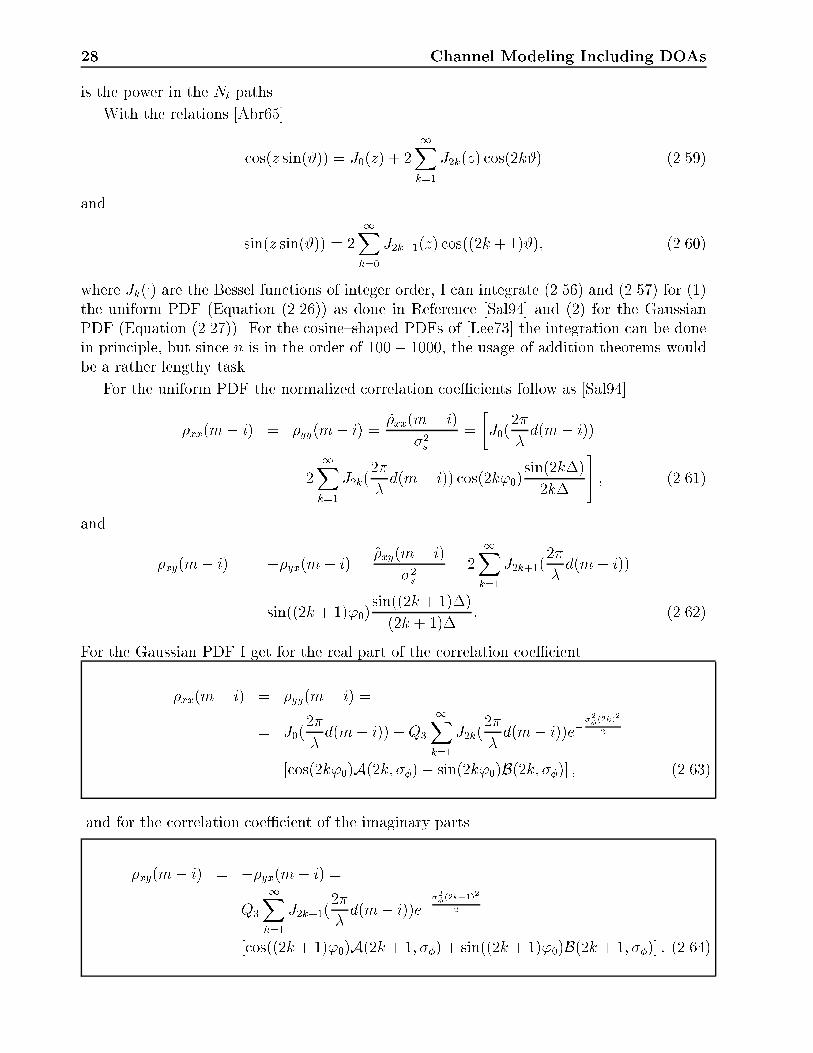
28 Channel Modeling Including DOAs
is the power in the Nl paths.
With the relations [Abr65]
cos(z sin(#)) = J0(z) + 21Xk=1
J2k(z) cos(2k#) (2.59)
and
sin(z sin(#)) = 21Xk=0
J2k+1(z) cos((2k + 1)#); (2.60)
where Jk(:) are the Bessel functions of integer order, I can integrate (2.56) and (2.57) for (1)
the uniform PDF (Equation (2.26)) as done in Reference [Sal94] and (2) for the GaussianPDF (Equation (2.27)). For the cosine{shaped PDFs of [Lee73] the integration can be donein principle, but since n is in the order of 100� 1000, the usage of addition theorems wouldbe a rather lengthy task.
For the uniform PDF the normalized correlation coe�cients follow as [Sal94]
�xx(m� i) = �yy(m� i) =~�xx(m� i)
�2s=
�J0(
2�
�d(m� i))
+21Xk=1
J2k(2�
�d(m� i)) cos(2k'0)
sin(2k�)
2k�
#; (2.61)
and
�xy(m� i) = ��yx(m� i) =~�xy(m� i)
�2s= 2
1Xk=1
J2k+1(2�
�d(m� i))
sin((2k + 1)'0)sin((2k + 1)�)
(2k + 1)�: (2.62)
For the Gaussian PDF I get for the real part of the correlation coe�cient
�xx(m� i) = �yy(m� i) =
= J0(2�
�d(m� i)) +Q3
1Xk=1
J2k(2�
�d(m� i))e�
�2�(2k)2
2
[cos(2k'0)A(2k; ��)� sin(2k'0)B(2k; ��)] ; (2.63)
and for the correlation coe�cient of the imaginary parts
�xy(m� i) = ��yx(m� i) =
Q3
1Xk=1
J2k+1(2�
�d(m� i))e�
�2�(2k+1)2
2
[cos((2k + 1)'0)A(2k + 1; ��) + sin((2k + 1)'0)B(2k + 1; ��)] : (2.64)

2.3 Low{Rank Channel Models 29
The quantities A(a; b) and B(a; b) are given by
A(a; b) = Re
�erf
��p8b� j
abp2
��� Re
�erf
�� �p
8b� j
abp2
��; (2.65)
and
B(a; b) = Im
�erf
��p8b� j
abp2
��� Im
�erf
�� �p
8b� j
abp2
��: (2.66)
erf(a+ jb) is the complex{valued error function. It can be calculated from
erf(x) = 1� e�x2
w(jx): (2.67)
The complex probability function w(x) is de�ned by [Abr65]
w(x) = e�x2
0@1 + 2jp
�
xZt=0
et2
dt
1A : (2.68)
Both tabulated values [Abr65] and a polynomial approximation [Hum82] for w(x) exist.
The envelope correlation coe�cient �env follows from the above results as [Lee94]
�env =Efxl;1mxl;1ig2 + Efxl;1myl;1ig2
Efx2l;1mg2= �2xx + �2xy; (2.69)
where the squares indicate that one considers powers. Figure 2.12 shows the envelope correla-tion coe�cient �env for various angles of incidence '0 and angular spreads S'. The correlationcoe�cient decreases with increasing angular spread and with decreasing angle of incidenceof the signals from array broadside, i.e. the direction perpendicular to the array axis. Themaxima are achieved at � = '0 = �90� and S' = 0�. Figure 2.13 compares the theoreticalpredicted correlation values (Equations (2.61) and (2.62)) with simulation results (accordingto Section 2.3). The PDF of the scatterers was assumed according to Equation (2.16). Thecurves agree well in their basic behavior.
The consequences of these correlation functions are twofold:
� If the angular spread is rather small the output signals of the elements of an BS antennaarray appear as strongly correlated. This enables the application of techniques todetermine the DOA from the knowledge of the array structure alone | the so{calledSR (Spatial Reference) techniques. I will address this topic in Chapter 3. However, ifthe �rst antenna element is in a fading dip, all others will be into the same dip too.Therefore the array provides no diversity gain at all in this situation.
� If the angular spread of a closed area is rather large, there exist no discrete{valuedDOAs and the signals of the di�erent elements of an BS antenna array appear as weaklycorrelated. The determination of DOAs is impossible (they are non{existent, in fact).However, the signals can be combined by using MRC (Maximal Ratio Combining).Since the fading on the di�erent elements is weakly correlated, the antenna is e�ectiveas diversity arrangement.

30 Channel Modeling Including DOAs
0
0
0
0
0
0
0.5
0.5
0.5
0.5
0.5
0.5
1.5
1.5
1.51 1
1.5
1.511
1
1
1
1
1
1
1
1
1.5
2
2
2
2
2
2
2.5
2.5
2.5
2.5
2.5
2.5
3
3
3
3
3
3
3.5
3.5
3.5
3.5
3.5
3.5
4
4
4
4
4
4
4.5
4.5
4.5
4.5
4.5
4.5
5
5
5
5
5
5
0
0
0
0
0
0
0.2
0.2
0.2
0.1
0.1
0.1
0.2
0.1
0.1
0.2
0.2
0.1
0.3
0.3
0.3
0.3
0.3
0.3
0.4
0.4
0.4
0.4
0.4
0.4
0.5
0.5
0.5
0.5
0.5
0.5
0.6
0.6
0.6
0.6
0.6
0.6
0.7
0.7
0.7
0.7
0.7
0.7
0.8
0.8
0.8
0.8
0.8
0.8
0.9
0.9
0.9
0.9
0.9
0.9
ρenv
ρenv
ρenv
ρenv
ρenv
ρenv
d/λ
d/λ
d/λ
d/λ
d/λ
d/λ
Sϕ=1°
Sϕ=1°
Sϕ=1°
Sϕ=3°
Sϕ=3°
Sϕ=3°
Sϕ=3°
Sϕ=3°
Sϕ=3°
Sϕ=5°
Sϕ=5°
Sϕ=5°
Sϕ=5°
Sϕ=5°
Sϕ=5°
Sϕ=10°
Sϕ=10°
Sϕ=10°
Sϕ=10°
Sϕ=10°
Sϕ=10°
Sϕ=20°
Sϕ=20°
Sϕ=20°
Sϕ=20°
Sϕ=20°
Sϕ=20°
Sϕ=40°
Sϕ=40°
Sϕ=40°
Sϕ=40°
Sϕ=40°
Sϕ=40°
Sϕ=104°
Sϕ=104°
Sϕ=104°
Sϕ=52°
Sϕ=52°
Sϕ=52°
Sϕ=52°
Sϕ=52°
Sϕ=52°
(a)
(b)
(c)
Uniform PDF
of the scatterers around the MS
Gaussian PDF
ϕ0=0° ϕ0=0°
ϕ0=60° ϕ0=60°
ϕ0=90°ϕ0=90°
Figure 2.12: Envelope correlation coe�cient �env for various angles of incidence '0 versus thedistance of the antennas with the angular spread S' as parameter. (a) '0 = 0�, (b) '0 = 60�,and (c) '0 = 90�.
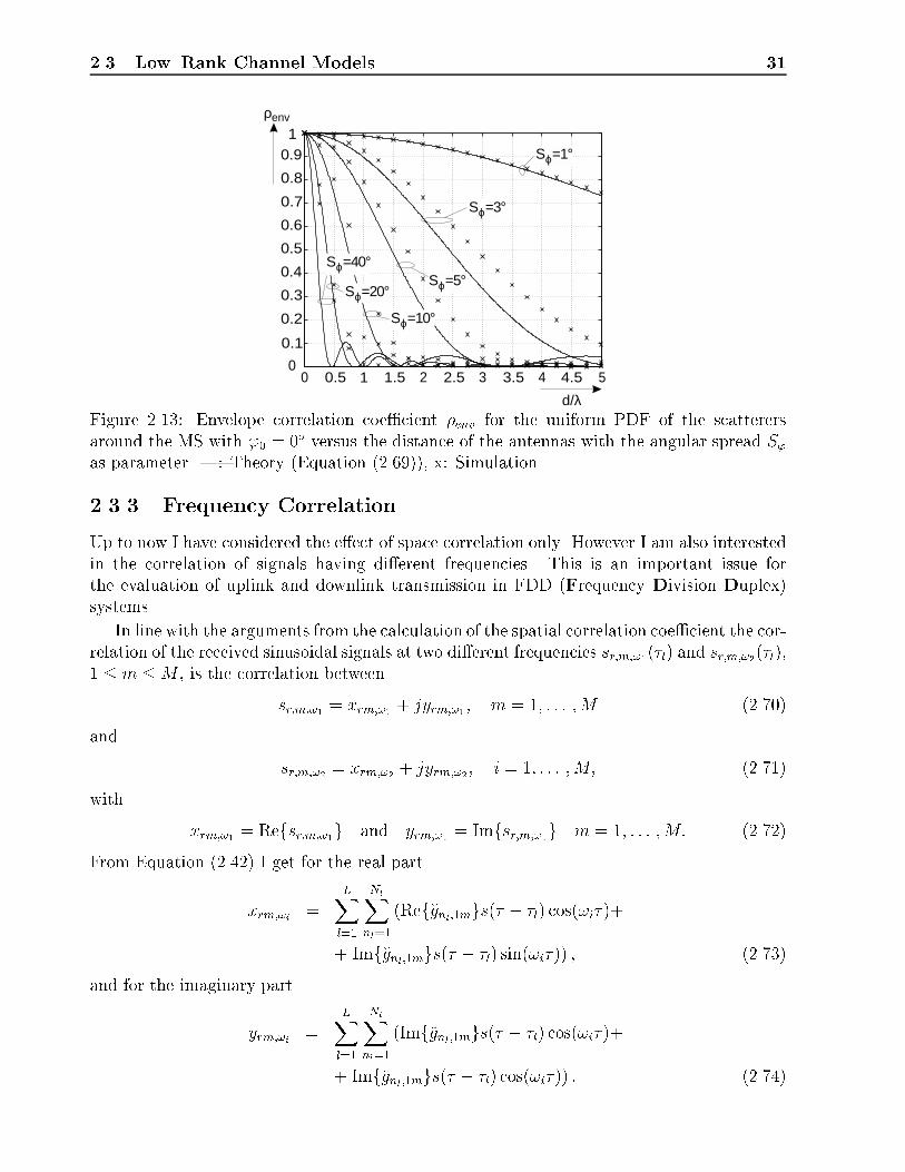
2.3 Low{Rank Channel Models 31
0 0.5 1.51 2 2.5 3 3.5 4 4.5 50
0.2
0.1
1
0.3
0.4
0.5
0.6
0.7
0.8
0.9
ρenv
d/λ
Sϕ=1°
Sϕ=3°
Sϕ=5°
Sϕ=10°
Sϕ=20°
Sϕ=40°
Figure 2.13: Envelope correlation coe�cient �env for the uniform PDF of the scatterersaround the MS with '0 = 0� versus the distance of the antennas with the angular spread S'as parameter. |: Theory (Equation (2.69)), x: Simulation.
2.3.3 Frequency Correlation
Up to now I have considered the e�ect of space correlation only. However I am also interestedin the correlation of signals having di�erent frequencies. This is an important issue forthe evaluation of uplink and downlink transmission in FDD (Frequency Division Duplex)systems.
In line with the arguments from the calculation of the spatial correlation coe�cient the cor-relation of the received sinusoidal signals at two di�erent frequencies sr;m;!1(�l) and sr;m;!2(�l),1 � m �M , is the correlation between
sr;m;!1 = xrm;!1 + jyrm;!1; m = 1; : : : ;M (2.70)
and
sr;m;!2 = xrm;!2 + jyrm;!2; i = 1; : : : ;M; (2.71)
with
xrm;!1 = Refsr;m;!1g and yrm;!1 = Imfsr;m;!1g m = 1; : : : ;M: (2.72)
From Equation (2.42) I get for the real part
xrm;!i =LXl=1
NlXnl=1
(Ref�gnl;1mgs(� � �l) cos(!i�)+
+ Imf�gnl;1mgs(� � �l) sin(!i�)) ; (2.73)
and for the imaginary part
yrm;!i =LXl=1
NlXnl=1
(Imf�gnl;1mgs(� � �l) cos(!i�)+
+ Imf�gnl;1mgs(� � �l) cos(!i�)) ; (2.74)
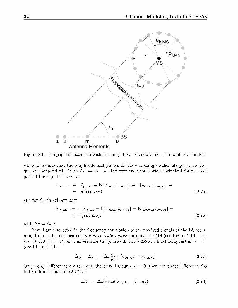
32 Channel Modeling Including DOAs
ϕ0
ϕk,MS
BS
Antenna Elements1 2 Mm
ϕi,MS
Propagation Medium
MS
rMS
r
Figure 2.14: Propagation scenario with one ring of scatterers around the mobile station MS.
where I assume that the amplitude and phases of the scattering coe�cients �gnl;1m are fre-quency independent. With �! = !2 � !1 the frequency correlation coe�cient for the realpart of the signal follows as
~�xx;�! = ~�yy;�! = Efxrm;!1xrm;!2g = Efyrm;!1yrm;!2g == �2s cos(��); (2.75)
and for the imaginary part
~�xy;�! = ��yx;�! = Efxrm;!1yrm;!2g = Efyrm;!1xrm;!2g == �2s sin(��); (2.76)
with �� = �!� .
First, I am interested in the frequency correlation of the received signals at the BS stem-ming from scatterers located on a circle with radius r around the MS (see Figure 2.14). ForrMS � r; 0 < r � R; one can write for the phase di�erence �� at a �xed delay instant � = �1(see Figure 2.14)
�� = �!�1 ��!r
ccos('nl;MS � 'nl;BS): (2.77)
Only delay di�erences are relevant, therefore I assume �1 = 0, then the phase di�erence ��follows from Equation (2.77) as
�� = ��!rccos('nl;MS � 'nl;BS): (2.78)

2.3 Low{Rank Channel Models 33
The correlation coe�cients become
�xx;�! =~�xx;�!�2s
=
2�Z0
cos(�!r
ccos('nl;MS � 'nl;BS)) d'nl;MS (2.79)
and
�xy;�! =~�xy;�!�2s
= �2�Z0
sin(�!r
ccos('nl;MS � 'nl;BS)) d'nl;MS; (2.80)
where I assume that the scatterers are equally distributed in angle around the MS.
By applying the identities
cos(z cos(#)) = J0(z) + 21Xk=1
(�1)kJ2k(z) cos(2k#) (2.81)
and
sin(z cos(#)) = 21Xk=0
(�1)kJ2k+1(z) cos((2k + 1)#); (2.82)
I can integrate Equations (2.79) and (2.80). For the real parts I get
�xx;�! = J0
��!
r
c
�; (2.83)
and for the imaginary parts
�xy;�! � 0: (2.84)
These results agree with Reference [Kal96]. Therefore the sum correlation coe�cient �r;�! isequal to the square of the correlation coe�cient of the real parts �2xx;�!,
�r;�! = �2xx;�! + �2xy;�! = �2xx;�!: (2.85)
This correlation coe�cient holds only for scatterers arranged in a circle with constant radiusr around the mobile. By introducing PDFs for the scatterers around the mobile an averagecorrelation coe�cient can be determined. It is calculated for the uniform PDF as
��! =
0@ 1
R2�
2�Z'=0
RZr0=0
r0J0
��!
r0
c
�dr0d'
1A
2
=
=
�2c
R�!J1
��!R
c
��2; (2.86)

34 Channel Modeling Including DOAs
0 00.2 0.20.6 0.61
1 1
10.8 0.80.4 0.41.2 1.21.4 1.40 0
0.2
0.1
0.2
0.1
0.3 0.3
0.4 0.4
0.5 0.5
0.6 0.6
0.7 0.7
0.8 0.8
0.9 0.9
ρ∆ω ρ∆ω
∆f/f0 (%) ∆f/f0 (%)
R=10λ
R=10λR=20λ
R=20λ
R=100λ R=100λ
R=400λ R=400λR=50λ
R=50λ
(a) (b)
Figure 2.15: Frequency correlation ��! versus the normalized frequency separation �f=f0with the radius R of the scattering circle as parameter. |: Theory, x: Simulations. (a)Uniform PDF for the scatterers around the MS, (b) Gaussian PDF for the scatterers aroundthe MS. The curve for R = 400� was not tested by simulation, since the time requirementsto get a reliable result would have been too large.
and for the Gaussian PDF as
��! =
0@ 1
2�R2
2�Z'=0
1Zr0=0
r0e�(r0)22R2 J0
��!
r0
c
�dr0d'
1A
2
=
= e��R�!p2c
�4: (2.87)
Figure 2.15 shows the frequency correlation ��! for di�erent radii R of the scattering circle.The correlation increases with decreasing radius R of the scattering circle. The fading of twosignals at di�erent frequencies is considered as "uncorrelated", if ��! � 0:5. For a scatteringcircle with R = 100�, the fading of two signals that are separated by at least 0:26% (0:14%)of the center frequency for the uniform PDF (Gaussian PDF) are uncorrelated. Reference[Fle90] showed two signals at di�erent frequencies as uncorrelated if �f � 1=(2�S), whereequality holds for the exponentially shaped PDP [Jak74]. By simulation, for a radius of thescatterer circle of R = 100� for a frequency f0 = 1800MHz the delay spreads for the uniformPDF (Gaussian PDF) are found as S = 34:1ns (S = 52:8ns). This leads to values for thenormalized frequency separation of �f=f0 = 0:26% (�f=f0 = 0:17%) for the uniform PDF(Gaussian PDF). These values agree well with the ones found by applying my theory.
The simulated curves show good agreement with theory down to a correlation of 0.2. Theremaining correlation in the simulation results might be due to the �nite number of scatterersin my simulations.
For the same radius R of the scatterer circle the assumption of a Gaussian PDF for thescatterer locations gives lower correlation values. This is evidently, since the scatterers arespread out more widely than for the Uniform PDF.

2.3 Low{Rank Channel Models 35
2.3.4 Line{Of{Sight Components
Up to now I have considered a NLOS channel only. However, in mobile communications wealso have parts of time LOS, quasi{LOS, or obstructed LOS [Kar95]. To corporate an LOSpath with its associated behavior over time, a propagation path for the direct connectionbetween MS and BS is assigned. This propagation path is subject to shadowing. Usually itsamplitude gLOS has a log{normal statistic [Jak74]
p(ln(gLOS)) =1p
2��2LOSe� (ln(gLOS)�ln(gLOS))2
2�2LOS ; gLOS > 0; (2.88)
where gLOS is the (linear) mean value of the received LOS amplitude, �LOS is the standarddeviation, and ln(:) denotes the natural logarithm.
The time behavior of the LOS contribution may be modeled by a simple �lter. The inputsignal s(�) to the �lter with impulse response h(�) is a sequence of arbitrary distributed,statistically independent, i.e. their ACF (AutoCorrelation Function) is a �{pulse, randomnumbers. Due to the central limit theorem, the output signal
ln(gLOS(�)) = (s � h)(�); (2.89)
where � denotes convolution, is a sequence of Gaussian random variables having an ACFgiven by
rln(gLOS)(�) = rh(�); (2.90)
where rh(�) is the ACF of the impulse response of the �lter h(�) [Wei91].
A typical model for the correlation properties is an exponentially decreasing correlationfunction [Gud91], [Gia96]. It is given by
rln(gLOS)(�) = (rg � fg)(�)
= �2LOS
1Z�1
e��k�kfg(�� �) d�; (2.91)
with
rd(i) = �2LOSe��d0kik; (2.92)
and
fg(�) =1
Cp��2r
e��2
�2r : (2.93)
rd(i) is the exponential correlation model for the correlation with i as a discrete{time variable.The parameter e�� is the correlation coe�cient between two points spaced by a distance d0, �is a continuous valued space variable, �r is a shape parameter, and C is a normalization factor,de�ned to ensure r(0) = �2LOS. If �r tends to zero, r(�) degenerates into the exponentialmodel [Gia96].

36 Channel Modeling Including DOAs
The power in the LOS{component in relation to the power in the NLOS{components canbe adjusted by introducing the Rice{factor [Rap96]
KRice(dB) = 10 log10
0BBB@kgLOSk
2
LPl=1
kglk2
1CCCA : (2.94)
2.3.5 The Moving Scatterer Model
Let us now consider an MS moving through a scatterer scenario. Some local scatterers get outof range and some new local scatterers will appear. The appropriate model to take this e�ectinto account is the moving scatterer model. Its principle is given by the following algorithm,which can be used to generate this model:
1. For the time instant t = t1, place N scatterers around the location rMS = [xMS; yMS]T
of the MS according to Equation (2.16). It is assumed that N is kept constant duringthe simulation.
2. At the time instant t2 the MS has moved to the position rMS;2 = rMS+[vMS;x; vMS;y]T (t2�
t1).
3. Draw a new scatterer circle with its center at the new location of the MS, rMS;2. Removeall scatterers outside the new scatterer circle. Their number be N1.
4. If N1 = 0 go back to Step 2 for the next time instant.
5. If N1 > 0, N new scatterers are generated within the new scattering area in accordanceto the PDF of Equation (2.16). The N1 scatterers with the largest projection onto theline connecting rMS and rMS;2 are added to the model (see Figure 2.16). Go back toStep 2.
2.4 High{Rank Channel Models
In environments with large delay spreads and/or large angular spreads the channel modelintroduced so far is not applicable. High{rank channel models taking into account di�erent(local) scattering scenarios and time dispersion are needed.
I propose two ways of generating high{rank channel models:
� Superposition of Low{Rank Channels: Combine a number of low{rank channelsto achieve large delay and angular spreads. An example is given in Figure 2.17. Here,two angular sections with scatterers exist, giving rise to time dispersion and to a largeangular spread. Additional discrete re ectors (in the far �eld of the BS antenna) may beintegrated into the model. This is especially important for urban areas, where high{risebuildings may cause signi�cant re ections [Li96].

2.4 High{Rank Channel Models 37
MSTime instant t1
MSTime instant t2
vMS
rMS
rMS,2
BS
Antenna elements
Scatterers valid for t=t1Scatterers valid for t=t1 and t=t2Scatterers valid for t=t2
1 2 Mm
∆ϕ
Figure 2.16: Principle of the moving scatterer model. Two consecutive time instants t1 andt2 are shown. Six scatterers active at time instant t1 are outside the scatterer circle for thetime instant t2. These scatterers are removed and six new scatterers are added. Note thatnot all of the new scatterers have to be within the area spanned by the second scatterer circlealone.
BS-Antenna
Power Delay ProfilePhysical Channel Model
LocalScatterers
P(τ)
τ
MS
DistantScatterers
DistantScatterers
DiscreteReflector
DiscreteReflector
∆ϕs
Figure 2.17: Exemplary high{rank channel model. Local scatterers, distant scatterers and adiscrete re ector exist. The power delay pro�le clearly resembles the di�erent contributions.
38 Channel Modeling Including DOAs
� Heavy Local Scattering around the BS: I consider two possible ways of modelinglocal scattering around the BS:
{ A scatterer circle around the BS antenna. This is most appropriate for microcells,where the antennas are located below rooftop level. Figure 2.19 shows an examplefor such a scenario. The scatterers are both around the MS and the BS antenna.
{ A scattering region may encompass both BS and MS (Figure 2.19), as it is mostlikely for picocells and low{range indoor wireless communications.
According to Ref. [Ott96], another important case arises even in propagation environmentswith low{rank characteristics. If the propagation time of the received signal across the array isin the same order as the symbol time of the received signal, one also needs high{rank channelmodels [Ott96]. However, consider an antenna array operating at frequency f0 having Melements spaced by d = �=2. Then the maximum propagation time across the array is givenby �p;max = (M�1)d=c0. Systems having symbol times in the order of �p;max require a relativebandwidth in the order of Brel = B=f0 = 1=(M � 1). Reasonable antenna sizes in mobilecommunications are, from my point of view, typically in the order of M = 10 elements.This system would therefore require a relative bandwidth of 10% for one channel. This isfar beyond the bandwidth allocations of today's and next generation mobile communicationssystems. Therefore I do not further consider the possibility of propagation times across thearray to be in the order of the symbol time.
2.5 Parameters for Channel Models
This chapter proposes several channel models for performance assessment of mobile commu-nications systems. Parts of the proposals are in line with the ones from [Bla95], [Bla96] and[Egg96], but they have novel features. These features are
� models for all cellular environments, as opposed to [Egg96], where only certain modeltypes are proposed,
� a signi�cant smaller number of scatterers as the models proposed in [Bla95], makingthem computationally more attractive,
� varying distances between MS and BS, as opposed to [Bla95], where the distances arekept �xed,
� the moving scatterer model to incorporate for larger movements of the MS,
� averaged angular power spectra for all models.
Figure 2.18 gives an overview of my proposal for channel models for low{rank channels. Theangular spectra are to be interpreted as mean values of the incident power versus the angulardirection, i.e. they are averaged over a large number of instantaneous spectra. They consistbasically of the local scatterer model around the MS associated with a LOS component

2.5ParametersforChannelModels
39
Local ScatteringModel
Low-RankChannel Models
without LOSwith LOS
Typi
cal A
ngul
ar S
pect
raS
patia
l Cha
nnel
Mod
el
with Local Scatteringat the BS
with Local Scatteringat the BS
without Local Scatteringat the BS
without Local Scatteringat the BS
ϕ/deg.ϕ/deg. ϕ/deg.ϕ/deg.
0 0 00
30 30 3030
6060 6060
9090 9090
120 120 120120
150150 150150
180180 180180210
210 210210
240240 240240
270270 270270
300300 300300
330330 330330
Rec
eive
dP
ower
(dB
)
Rec
eive
dP
ower
(dB
)
Rec
eive
dP
ower
(dB
)
Rec
eive
dP
ower
(dB
)0 0 00
-20 -20 -20-20
-40 -40 -40-40
-60-60 -60-60
BS-AntennaBS-Antenna
r1
r2
BS-Antenna BS-Antenna
MSMS MS MS
Figu
re2.18:
Channelmodels
forlow
{rankchannels.

40 Channel Modeling Including DOAs
Property Dimensions
Radius R of the localscattering circle (for BS & MS)
100� � R � 300�
Number Ns of local scatterers Ns � 10PDF of the angle 'scatof the local scatterers
p('scat) = 1=(2�); 0 < 'scat � 2�
PDF of the distance r of p1(r) =1
R2�; kr � rMSk � R
the local scatterers to the MS p2(r) =1
2�R2e�
(r�rMS)2
2R2
Damping factor of thelocal scatterer al
p(al) = UD(0:5; 1=p12)Signal power from the local scatterers �2alPDF of the phase shifts �lintroduced by the local scatterers
p(�l) = 1=(2�); 0 < �l � 2�
Inner cell radius r1 r1 � ROuter cell radius r2 r2 � 90000�PDF of the distance rMS
between BS and MSp(rMS) = 2rMS=(r
22 � r21); r1 � rMS � r2
Power in the LOS{component KRice = 0� 30 dBFading statistic of the
LOS{component gLOS p(ln(gLOS)) =1p
2��2LOSe� (ln(gLOS)�ln(gLOS))2
2�2LOS
Time behavior of the fading rh(�) = �21R
�1e��k�kfg(�� �) d�
PDF of the angle 'l;BSof the local scatterers at the BS
p('l;BS) = 1=(2�); 0 < 'l;BS � 2�
Power of the local scatterers�2al around the BS
�2al � (40� 60)dB
Table 2.1: Parameters for the local scatterer model.

2.5 Parameters for Channel Models 41
and/or local scattering around the BS. The parameters for these models are summarized inTable 2.12.
The values given for the local scatterer model form also the base for high{rank channelmodels, since the local scatterer model is often a main component of these model types.Figure 2.19 gives an overview over the di�erent cell geometries and the appropriate scatteringmodels.
2.5.0.1 Macrocells
The model for macrocells is simply a linear combination of local scatterer models. Typicallytwo scatterer scenarios are assigned to one MS. This is due to the reason that by calculatingthe doppler spectra from the spatial component, the model should fall back to the COST207models [Cos89]. The canonical model consists of one local scattering scenario around themobile and the other away from the mobile | distant scatterers. The angle between thescatterer scenarios can be chosen according to an arbitrary distribution. The distances arechosen according to the distribution functions for the local scatterer model. Additionally thedelay has to be monitored to get reasonable models. E.g. for the bad urban area the delayof the second component should be around 5 �s and for the hilly terrain the delay should bearound 15�s. Additionally to the scattering scenarios, discrete DOAs can be incorporatedinto the model. This is important for urban areas with high{rise buildings. The parametersfor the model are given in Table 2.2.
2.5.0.2 Microcells
Microcells are characterized by antennas below the rooftops. This means that local scatteringaround the BS cannot be neglected. Additionally the distances rMS between BS and MS areat least by an order of magnitude less than for macrocells.
I distinguish between LOS microcells and NLOS microcells. Due to the below{rooftopantennas the DOAs are mostly con�ned to the directions of the streets around the BS. Thediameter of the scatterer circle is mainly determined by the width of the streets. NLOSmicrocells can be characterized by scattering scenarios at the street crossings with LOS tothe BS, where the waves are guided to the MS. The DOA spectrum is more uniform than formacrocells. The parameters of the model are summarized in Table 2.2.
2.5.0.3 Picocells
In picocells, the DOA spectrum can approach isotropy [Egg95a], [Ott96]. The scatteringcircle usually encompasses both MS and BS due to the small distances between BS andMS. If there is a LOS component, the DOA spectrum would of course be biased into itsdirection, but the angular spread is larger than for the other environments [Egg95a]. Themodel parameters can be found in Table 2.2. Of course, all scattering coe�cients have tobe weighted by the pattern of a single antenna element to take its directional behavior intoaccount.
2In rural and suburban macrocell scenarios the radius R might be independent of the wavelength andmuch larger than the values given here. Detailed measurements to determine the possible range for R arenecessary.

42
ChannelModelingInclu
dingDOAs
High-RankChannel Models
PicocellsMacrocells Microcells
Typi
cal A
ngul
ar S
pect
ra
Linear Combination ofLocal Scattering Modelsand Discrete Reflectors
without LOS without LOSwith LOS with LOS
ϕ/deg. ϕ/deg.ϕ/deg. ϕ/deg.
ϕ/deg.
ϕ/deg.
00 00 03030 3030 30
6060 6060 60
9090 9090 90
120120 120120 120
150150 150150 150180180 180180 180
210210 210210 210
240240 240240 240
270270 270270 270
300300 300300 300
330330 330330 330
Rec
eive
dP
ower
(dB
)
Rec
eive
dP
ower
(dB
)
00 0
-20 -20-20 -20
-40 -40-40 -40
-60-60 -60-60 -60
Rec
eive
dP
ower
(dB
)
Rec
eive
dP
ower
(dB
)-20
-40
Rec
eive
dP
ower
(dB
)
0
Spa
tial C
hann
el M
odel
BS-Antenna BS-Antenna
BS-AntennaBS-Antenna
BS-Antenna
MS
MS MSMSMS
DistantScatterers
DiscreteReflector
∆ϕs
0
Figu
re2.19:
Channelmodels
forhigh
{rankchannels.

2.5 Parameters for Channel Models 43
Property Dimensions
MacrocellsParameters for the as for low{ranklocal scatterer models channelsNumber Ns of localscattering scenarios
Ns = 2
PDF of the angular distance �'sbetween two scattering scenarios
p(�'s) = 1=(q1 � q2); 0 � q2 < q1 � �
Number Ndiscr of discretere ectors
0 � Ndiscr � 4
PDF of the angle 'l;BSof the local scatterers at the BS
p('l;BS) = 1=(2�); 0 < 'l;BS � 2�
Power of the local scatterers�2al around the BS
�2al � (40� 60)dB
MicrocellsRadius R of the localscattering scenario
R = wStreet=2
Number Ns ofscatterers
Ns � 10
Inner cell radius r1 � 0:5ROuter cell radius r2 � 3000�
p('l) =
�k1=i if 0 < k'l � 'ik � �=Smk2 elsewhere
Sm = 16; 'i = �(i� 1)2�=Sm; 1 � s � Sm=2PDF p('l) of the DOA i = 1; : : : ; s; k2 = 0:1618; �s = 1 +Ps
i=2 2=ik1 = Sm=�s(1=(2�)� k2(1� (2s� 1)=(2Sm)))
PDF of the angle 'l;BSof the local scatterers at the BS
p('l;BS) = 1=(2�); 0 < 'l;BS � 2�
Power of the local scatterers�2al around the BS
�2al � (20� 40)dB
PicocellsRadius R of the localscattering scenario
R = wRoom=2
Number Ns ofscatterers
Ns � 10
Inner cell radius r1 � 0:1ROuter cell radius r2 � 200�
p('l) = k1 cos(k2'l);�� � 'l � �PDF p('l) of the DOA k1 = 0:4206, k2 = 0:4PDF of the angle 'l;BSof the local scatterers at the BS
p('l;BS) = 1=(2�); 0 < 'l;BS � 2�
Power of the local scatterers�2al around the BS
�2al � (10� 20)dB
Table 2.2: Parameters for high{rank channel models.

44 Channel Modeling Including DOAs
2.6 Discussion
Typical "angular spreads" appearing in literature are 2��7� [Zol96b], [Tru96]. Ref. [Zol96b]claims they are measured, without given details of the measurements. Ref. [Tru96] hasassumed a Gaussian distribution of the incident signals around their nominal DOA. Theangular spread was determined by �tting the parameters mean, �, and standard deviation, �'from measured data. Ref. [Mar96a] has actually measured scenarios in Frankfurt, Germanyand determined the angular spread to be around 5� � 11�. Bear in mind, though, that the�rst authors de�ne the angular spread di�erently from this work. They can be convertedto my results by using Equation (2.28). This leads to angular spreads of 0:6� � 2� for theuniform PDF and also 2� � 7� for the Gaussian PDF.
Based on these measurements the results for the spatial correlation values show that ifthere is a fading dip, the whole array will be in this dip | with reasonable array sizes formobile communications, Md = 5� (M = 10 and d=� = 0:5). Consequently countermeasureshave to be taken:
� Space Diversity: A second smart antenna is mounted so far away from the �rst thatsu�cient decorrelation of the signals is achieved. From my point of view, this is a ratherimpracticable solution due to the huge space, hardware, and mounting requirements.
� Polarization Diversity: Two antennas are used in each position. One is sensitiveto the horizontal, the other to the vertical polarized part of the incoming wave. Thissolution does not necessarily increase the size of the antenna array. If special antennaelements like circular microstrip patch antennas are used, they can receive two orthog-onal polarizations and provide polarization diversity. Of course, they need two feedpoints to achieve this.
The frequency correlation is an important issue to deal with in FDD systems, like GSMand DCS 1800. For the duplex distances used in these systems (GSM: 45 MHz, DCS 1800:95 MHz) the short{term fading in NLOS situations is uncorrelated. This is important fordownlink (BS transmits, MS receives) beamforming based on information of the uplink (MStransmits, BS receives). The results of this chapter show that for NLOS the optimum antennapatterns for the uplink cannot be used directly in the downlink of an FDD system.
The generic channel models presented in this chapter are a �rst step towards a method-ology of channel models including a spatial component. Such a methodology is neededespecially for the determination of e�cient processing schemes and performance assessmentof proposed system architectures.

Chapter 3
Adaptation Algorithms|An Overview
This chapter describes possible algorithms for weight adaptation of smart antennas. Toexploit the full potential of smart antennas, advanced techniques for processing the receivedand transmitted signals are necessary. Suitable algorithms for similar problems like direction�nding, jammer location and anti{jamming measures were investigated in the �elds of radarand sonar. All these algorithms are candidates for the use in a mobile communicationssystem. Therefore they have to be evaluated and their performance tradeo�s have to beexamined.
3.1 Basics
The crucial point for the use of such algorithms in a mobile communications system are
� the system requirements: Only small antenna arrays (M in the order of some tens)can be utilized in mobile communications systems, since the system should be coste�ective | there is one transceiver necessary for each of the M elements | and theantenna should not require too much space. This is in contrast to radar applications,where antennas with M in the order of some thousands can be applied. Since M is sosmall, the algorithm requirements are much more severe in a mobile communicationssystem;
� the propagation channel: The directional nature of the mobile radio channel wasalready discussed in Chapter 2. The DOAs are not discrete, instead they are spread outin angle. This limits the performance of algorithms developed under the assumption ofdiscrete DOAs. Furthermore, in mobile communications the algorithms have to copewith much more multipath than in most radar applications;
� the air interface protocol: The speci�ed | or, to be speci�ed | air interface pro-tocol for 2nd and 3rd generation mobile communications systems de�nes the boundaryconditions for the algorithms. As example, systems utilizing FDD require in general dif-ferent algorithmic strategies for serving the uplink and the downlink as a TDD{system,as I will show in Chapter 8. The a{priori knowledge of training sequences should beexploited. The time variance of the channel during a data burst has to be considered,at least for systems like D{AMPS (Digital Advanced Mobile Phone System) [Win96].
45

46 Adaptation Algorithms|An Overview
0 1 3 5 72 4 6
DataFlag
Tail bits Tail bitsFlag
DataTraining
3 57
4.615 ms
1 26
148 bits
156.25 bits (0.577 ms)
1 57 3
Frame
Timeslot
Figure 3.1: Basic TDMA frame, timeslot, and normal burst structure [Cme20]. The 26{bitmidamble is surrounded by 1 ag bit, 57 data bits, and 3 tail bits on each side.
For example, GSM is an FDD system. In NLOS{conditions the duplex separation islarge enough to give decorrelation of the uplink and the downlink channel (Chapter2), therefore the antenna pattern optimized for the instantaneous channel constellationon the uplink cannot be reused directly for downlink transmission. Another importantpart, the frame structure of the GSM{system, is shown in Figure 3.1. One timeslotcontains N = 148 bits. The essential part we are looking at is the 26{bit midamble,optimized for estimation of the channel impulse response for the application of a Viterbiequalizer. This sequence can also be used for separation (or distinction) of di�erentusers in the same timeslot and such serves as an identi�er. Each user must be given anunambiguous sequence, which serves not only as training sequence for adaptation of theantenna diagram, but also as user identi�cation. To clearly distinguish one user from theothers and to ease synchronization, the used training sequences rp (identi�ers) shouldshow a peak in their ACF and low values of the normalized periodic cross{correlationfunction
R(�) =1
S
SXs=1
rp(s)ro(s+ �1); 0 � � � S � 1; 1 � p; o � PTr; p 6= o;(3.1)
with
ro(s+ �1) =
�ro(s+ �) for s+ � � S
ro(s+ � � S) for s+ � > S; (3.2)
where PTr is the number of distinct sequences, and S is the length of each sequence.The used training sequences of the GSM system (full 26 bits) provide a relative auto-correlation peak of 5.4dB to 8.3dB, a maximum value of the relative cross{correlationof -2.3dB up to -6.7dB, and a mean value of the relative cross{correlation in the rangeof -13.2dB up to -17dB. Since the used sequences are optimized for channel impulseresponse determination, the cross{correlation values are non{optimum.

3.1 Basics 47
Optimum cross{correlation values can be achieved by the use of other families of train-ing sequences, e.g. Gold sequences [Sar80]. Having a length of 31 (25 � 1) bits, theyprovide a minimum relative autocorrelation peak of 10.7dB, a maximum value of therelative cross{correlation of -10.7dB, and a mean value of the relative cross{correlationof -16.8dB. This is a considerable improvement compared to GSM training sequences.However, with the use of Gold sequences, channel estimation at the mobile cannot bedone in such a simple and convenient way as with GSM training sequences.
3.1.1 Basic Principle
All algorithmic approaches are based on a BS antenna array. If a linear array is used, it willbe usually a horizontal one, since the horizontal angular spread of the incoming signals isusually (much) larger than the vertical for typical outdoor scenarios [Egg94], [Big95]. And, ofcourse, we want to concentrate the received/radiated energy to a speci�c azimuthal angularsection.
Here I consider only the case of a 1D{ULA (one{Dimensional Uniform Linear Array),but all my investigations and basic conclusions are also applicable to other array structureslike planar or circular arrays.
Let us take a look at the scenario depicted in Figure 3.2. There are k = 1; : : : ; K di�erentusers in the same frequency slot and in the same time slot. As explained in Chapter 1, incontrast to usual phased arrays, where beamforming is done at RF{level by controlling theamplitudes and phases of the feeding currents via attenuators and phase shifters, smartantennas are based on a �xed hardware part. The system "intelligence" is placed on theBB{level in digital signal processing circuits. This enables sophisticated algorithms to beapplied and gives a maximum amount of exibility. The BS signal processing unit has toseparate/combine K wanted signals from a linear combination of L (L � K) incident signalsat the array. Let x(�) be the array output data vector collected at time � . Then
x(�) = [x1(�); : : : xm(�); : : : ; xM(�)]T
=LXl=1
a('l)sl(�) + n(�)
= As(�) + n(�); (3.3)
where [:]T denotes the transpose, M is the number of antenna elements, 'l, 1 � l � L is theDOA of the l{th signal measured from array broadside, a('l) is the so{called array steeringvector corresponding to the l{th wave, A = [a('1); : : : ;a('L)] is the array steering matrix,s(�) = [s1(�); : : : ; sL(�)]
T , where sl(�), 1 � l � L is the l{th signal at an arbitrary referenceelement (usually element #1), and n(�) is additive white noise. The l{th incident signal slis given by
sl(�) = sk(� � �l); 1 � k � K; (3.4)
i.e. it is simply the transmitted signal of the k{th user with an appropriate time delay �l.
Assuming isotropic sensors and a 1D{ULA, the array steering vector corresponding to thek{th narrowband wave can be expressed as
a('l) = [1; e�j2�d sin('l)=�; : : : ; e�j2�(M�1)d sin('l)=�]T ; (3.5)

48 Adaptation Algorithms|An Overview
Data User1
Data User2
Data UserK
τ= Til
Pas
sban
d F
ilter
Dow
ncon
vert
er
Bas
eban
d F
ilter
Sam
pler
Ant
enna
Ele
men
ts
Sig
nal
proc
essi
ng
Antenna Signal processing
1
2
3
M
sr,1
sr,2
sr,3
sr,M
x1
x2
x3
xM
hPB(τ) hBB(τ)
User 1
User 2
User K
s1s2
sL-1
s3sl
sL
Figure 3.2: A typical mobile communications scenario. There are k = 1; : : : ; K di�erent usersin the same frequency slot and in the same time slot (SDMA). The BS signal processing unithas to separate/combine K wanted signals from a linear combination of L (L � K) incidentsignals at the array. The �xed antenna part and the signal processing unit are the two maincharacteristics of a smart BS antenna.
where � is the wavelength and d is the distance between two neighboring array elements.
To avoid ambiguities of the estimated directions of the users (spatial aliasing) | whichis especially important for the downlink | the spacing d must be less than or equal to �=2.
The actual array outputs might di�er from the model due to angle{dependent modelingerrors like near�eld e�ects, antenna pattern mismatch, and mutual coupling. This in uencesthe performance of the algorithmic approaches. These e�ects were addressed e. g. in [Ali93]and [Wei90].
The noise vector is given by n(�) = nI(�) + jnQ(�), where nI(�) (nQ(�)) denotes theinphase (quadrature) component of the thermal noise vector. It has zero mean and covariance
Efn(�1)n�(�2)g = �2IM�(�1 � �2); (3.6)
where IM denotes the M �M unity matrix and �2 is the noise power per antenna element.This implies that the noise is both temporally and spatially white. I will call this type ofnoise ST{AWGN (Spatio{Temporal Additive White Gaussian Noise).
The sample of x(�) at the time instant � = nT is given by
x(n) = x(� = nT ); (3.7)
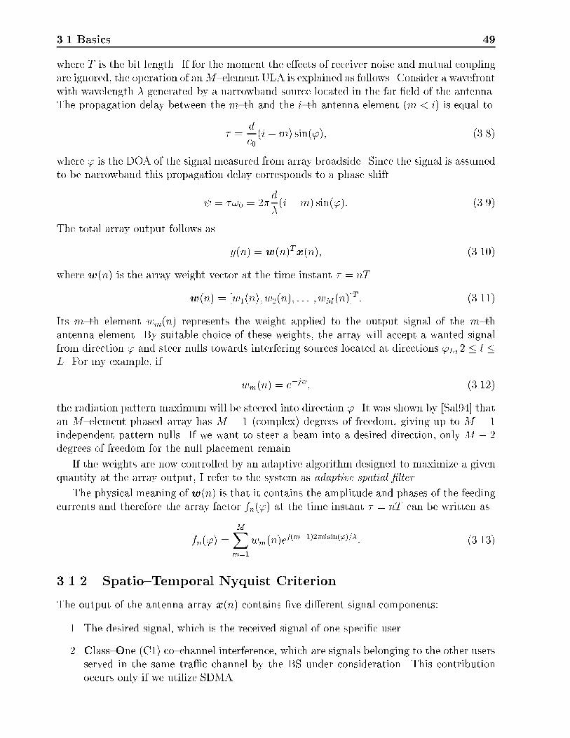
3.1 Basics 49
where T is the bit length. If for the moment the e�ects of receiver noise and mutual couplingare ignored, the operation of anM{element ULA is explained as follows. Consider a wavefrontwith wavelength � generated by a narrowband source located in the far �eld of the antenna.The propagation delay between the m{th and the i{th antenna element (m < i) is equal to
� =d
c0(i�m) sin('); (3.8)
where ' is the DOA of the signal measured from array broadside. Since the signal is assumedto be narrowband this propagation delay corresponds to a phase shift
= �!0 = 2�d
�(i�m) sin('): (3.9)
The total array output follows as
y(n) = w(n)Tx(n); (3.10)
where w(n) is the array weight vector at the time instant � = nT
w(n) = [w1(n); w2(n); : : : ; wM(n)]T : (3.11)
Its m{th element wm(n) represents the weight applied to the output signal of the m{thantenna element. By suitable choice of these weights, the array will accept a wanted signalfrom direction ' and steer nulls towards interfering sources located at directions 'L; 2 � l �L. For my example, if
wm(n) = e�j ; (3.12)
the radiation pattern maximum will be steered into direction '. It was shown by [Sal94] thatan M{element phased array has M � 1 (complex) degrees of freedom, giving up to M � 1independent pattern nulls. If we want to steer a beam into a desired direction, only M � 2degrees of freedom for the null placement remain.
If the weights are now controlled by an adaptive algorithm designed to maximize a givenquantity at the array output, I refer to the system as adaptive spatial �lter.
The physical meaning of w(n) is that it contains the amplitude and phases of the feedingcurrents and therefore the array factor fn(') at the time instant � = nT can be written as
fn(') =MXm=1
wm(n)ej(m�1)2�d sin(')=�: (3.13)
3.1.2 Spatio{Temporal Nyquist Criterion
The output of the antenna array x(n) contains �ve di�erent signal components:
1. The desired signal, which is the received signal of one speci�c user.
2. Class{One (C1) co{channel interference, which are signals belonging to the other usersserved in the same tra�c channel by the BS under consideration. This contributionoccurs only if we utilize SDMA.

50 Adaptation Algorithms|An Overview
3. Class{Two (C2) Interference, which is interference due to users served in other cells,
4. Adjacent channel interference due to users in the neighboring frequency bands, and
5. Noise.
In extension of [Ish95], [LeM90], and [Pro89] I de�ne a spatio{temporal Nyquist criterionthat must be met by received pulses if there is to be neither ISI (InterSymbol Interference)nor any C1 or C2 interference.
The condition for the received signal yk(n) for user k is given by
yk(n) = sk(n)�(� � nT )�('l � 'k); (3.14)
where sk(n); 1 � k � K is the amplitude and 'k is the DOA of the desired signal at the timeinstant � = nT , �(:) denotes the discrete{time Dirac delta{function, and
�('l � 'k) =
�1 for 'l = 'k; 1 � k � Kk
arbitrary elsewhere; (3.15)
where Kk denotes the number of DOAs belonging to user k. Usually signal components areincident from all directions at the receive antenna [Egg94], i.e. K = 1, and therefore theNyquist criterion becomes
yk(n) = sk(n)�(t� nT )�c('� 'k); (3.16)
with �c(:) denoting the continuous Dirac delta{function. This version of the spatio{temporal
Nyquist criterion is a discrete{time but continuous angle criterion.
The spatio{temporal Nyquist criterion includes the common temporal Nyquist criterion,if the dependence on the azimuthal angle ' is eliminated, i.e. there is only one antennaelement present, as in simple receivers.
3.2 Algorithms for Smart Antennas
Topologies of smart antennas may be subdivided into two general types | linear and nonlin-ear topologies. Associated with each type of smart antenna, there is one or more structuresfor implementing it. Moreover, for each structure there is a class of algorithms that maybe employed to adaptively adjust the smart antenna parameters according to a speci�edperformance criterion. Expanding Proakis' [Pro91] scheme for temporal equalization, Figure3.3 provides a categorization of smart antenna techniques for uplink reception into types,references, structures, and algorithms.
3.3 Linear Types
3.3.1 Temporal Reference (TR) Algorithms
TR (Temporal Reference) algorithms are well investigated approaches for mobile communi-cations systems [Win93], [Mun94], [Cor94]. Antenna systems based on TR algorithms are
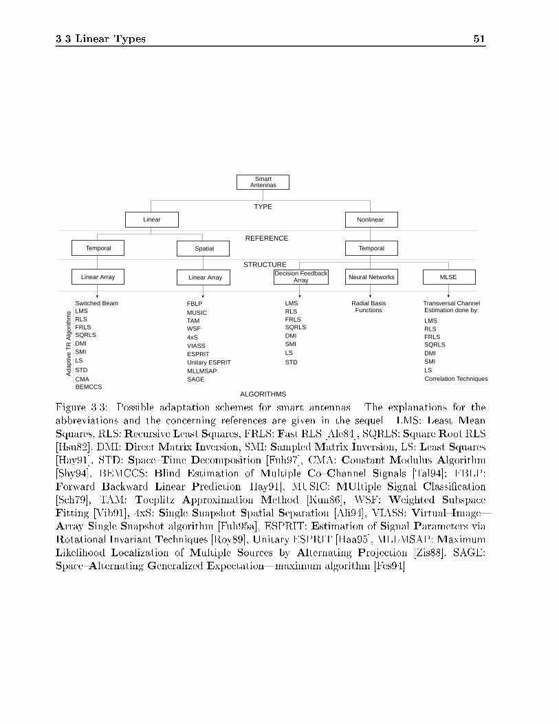
3.3 Linear Types 51
SmartAntennas
NonlinearLinear
Linear Array
Spatial
Linear Array
Temporal Temporal
LMSSwitched Beam LMS
LMS
SQRLS
Ada
ptiv
e T
R A
lgor
ithm
s
SQRLS
SQRLS
RLSRLS
RLS
SMISMI
SMI
DMIDMI
DMILS
LS
LSCorrelation Techniques
MUSIC
WSF
FBLP
TAM
4xSVIASS
MLLMSAPSAGE
Unitary ESPRITESPRIT
Decision FeedbackArray Neural Networks MLSE
Radial BasisFunctions
Transversal ChannelEstimation done by:
FRLSFRLS
FRLS
STD
CMA
STD
TYPE
ALGORITHMS
STRUCTURE
REFERENCE
BEMCCS
Figure 3.3: Possible adaptation schemes for smart antennas. The explanations for theabbreviations and the concerning references are given in the sequel. LMS: Least MeanSquares, RLS:Recursive Least Squares, FRLS: Fast RLS [Ale84], SQRLS: SquareRoot RLS[Hsu82], DMI: DirectMatrix Inversion, SMI: SampledMatrix Inversion, LS: Least Squares[Hay91], STD: Space{Time Decomposition [Fuh97], CMA: Constant Modulus Algorithm[Shy94], BEMCCS: Blind Estimation of Multiple Co{Channel Signals [Tal94]; FBLP:Forward Backward Linear Prediction [Hay91], MUSIC: MUltiple Signal Classi�cation[Sch79], TAM: Toeplitz Approximation Method [Kun86], WSF: Weighted SubspaceFitting [Vib91], 4xS: Single Snapshot Spatial Separation [Ali94], VIASS: Virtual{Image{Array Single Snapshot algorithm [Fuh95a], ESPRIT: Estimation of Signal Parameters viaRotational Invariant Techniques [Roy89], Unitary ESPRIT [Haa95], MLLMSAP:MaximumLikelihood Localization of Multiple Sources by Alternating Projection [Zis88], SAGE:Space{Alternating Generalized Expectation|maximum algorithm [Fes94].

52 Adaptation Algorithms|An Overview
often referred to as adaptive antennas. TR algorithms rely on knowledge about the time struc-ture of the desired received signal, e.g. the position and the structure of a known sequence(training sequence) or the knowledge of envelope properties of the signal to be received, todetermine the optimum antenna weights for reception of the desired signal and the rejectionof interference.
3.3.1.1 Signal Processing Structures
The mobile radio channel introduces multiplicative (fading) and dispersive (ISI) distortion.Additionally we have to cope with co{ and adjacent{channel{interference.
Conventional linear equalizers are bene�cial only in the case of ISI of duration less orequal to the time window the equalizer is designed for [Cos89]. Interfering signals are re-garded as additional colored noise. A linear time domain equalizer can do better againstco{channel interference than it can against the same level of noise [Pet90]. However, in doingso the linear equalizer only exploits the spectral characteristics of the interference throughits autocorrelation [Che92].
Antenna arrays are e�ective in overcoming
� Fading: To overcome fading, space diversity is most commonly used. By mountingat least two antennas far enough to achieve decorrelation (see also Chapter 2) of theincident signals and by applying suitable combination algorithms, system performanceis increased.
� Co{Channel Interference and Excessively Delayed Paths: An adaptive antennacan place nulls into directions, where co{channel interference and signals that are ex-cessively delayed are present.
Thus, time domain equalizer and adaptive arrays can be combined in a single adaptive processto combat the above mentioned e�ects impairing transmission over the mobile radio channel.
Figure 3.4 shows the array scheme for both temporal and spatial processing (equalization)| the wideband array scheme (spatio{temporal equalizer). It is designed for a widebandmobile radio channel, where we have to combat both ISI and fading. The narrowband arrayscheme (only space domain equalizer) can be derived from the wideband scheme by removingits temporal component (Rt = 1, see Figure 3.4). It is suited for a narrowband channel wheretransmission quality is impaired by at fading only.
For system performance it is of crucial importance to bring together these two techniquesto cope with a wideband mobile radio channel.
The output of a wideband array at time � = nT is given by
x(n) = [x1(n); : : : ; xM(n); x1(n� 1); : : : ;
xM (n� 1); : : : ; x1(n�Rt + 1); : : : ; xM(n� Rt + 1)]T ; (3.17)
where M is the number of antenna elements and Rt is the number of taps at each antennaelement. The weight vector is given by
w(n) = [w11(n); : : : ; wM1(n); w12(n); : : : ;
wM2(n); : : : ; w1Rt(n); : : : ; wMRt(n)]T : (3.18)

3.3 Linear Types 53
TT T
TT T
T T T
T T T
Combiner
Adaptationalgorithm
+
Training sequence
Output y(n)
Weightadaptation
orsliced output
-
w21(n)
x2(n)
w22(n)
w31(n)
x3(n)
w32(n)
wM1(n)
xM(n)
wM2(n) wM3(n)wMRt
(n)
w3Rt(n)
w2Rt(n)
w1Rt(n)
w11(n)
x1(n)
w12(n) w13(n)
w23(n)
w33(n)
τ=nT
1-st temporalstage
Rt-th temporalstage
Ant
enna
1
2
3
M
Figure 3.4: Wideband array scheme for both spatial and temporal processing. During theduration of the training sequence the ideal sequence is used for weight adaptation, afterwardsthe sliced outputs may be utilized for channel tracking. The combiner might be a simple adderor a more sophisticated MRC (Maximal Ratio Combiner).
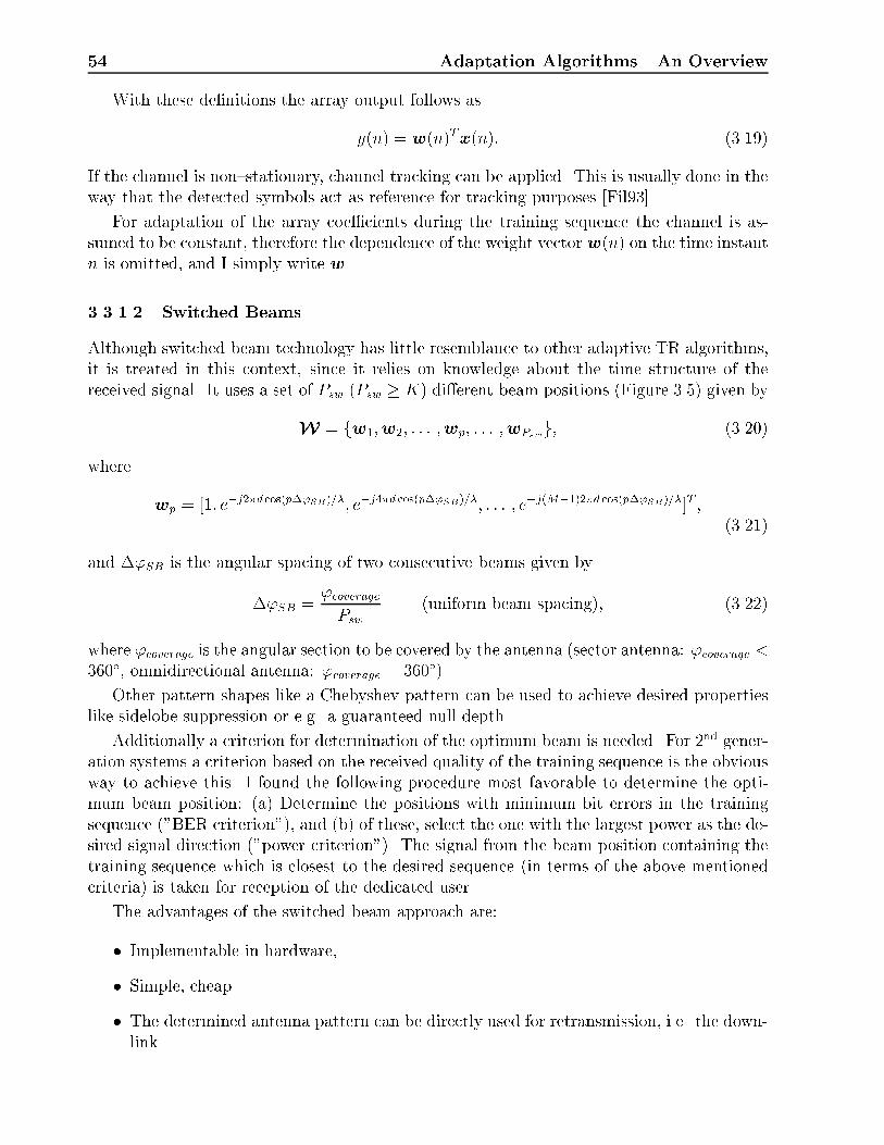
54 Adaptation Algorithms|An Overview
With these de�nitions the array output follows as
y(n) = w(n)Tx(n): (3.19)
If the channel is non{stationary, channel tracking can be applied. This is usually done in theway that the detected symbols act as reference for tracking purposes [Fil93].
For adaptation of the array coe�cients during the training sequence the channel is as-sumed to be constant, therefore the dependence of the weight vector w(n) on the time instantn is omitted, and I simply write w.
3.3.1.2 Switched Beams
Although switched beam technology has little resemblance to other adaptive TR algorithms,it is treated in this context, since it relies on knowledge about the time structure of thereceived signal. It uses a set of Psw (Psw � K) di�erent beam positions (Figure 3.5) given by
W = fw1;w2; : : : ;wp; : : : ;wPswg; (3.20)
where
wp = [1; e�j2�d cos(p�'SB)=�; e�j4�d cos(p�'SB)=�; : : : ; e�j(M�1)2�d cos(p�'SB)=�]T ;(3.21)
and �'SB is the angular spacing of two consecutive beams given by
�'SB ='coveragePsw
(uniform beam spacing); (3.22)
where 'coverage is the angular section to be covered by the antenna (sector antenna: 'coverage <360�, omnidirectional antenna: 'coverage = 360�).
Other pattern shapes like a Chebyshev pattern can be used to achieve desired propertieslike sidelobe suppression or e.g. a guaranteed null depth.
Additionally a criterion for determination of the optimum beam is needed. For 2nd gener-ation systems a criterion based on the received quality of the training sequence is the obviousway to achieve this. I found the following procedure most favorable to determine the opti-mum beam position: (a) Determine the positions with minimum bit errors in the trainingsequence ("BER criterion"), and (b) of these, select the one with the largest power as the de-sired signal direction ("power criterion"). The signal from the beam position containing thetraining sequence which is closest to the desired sequence (in terms of the above mentionedcriteria) is taken for reception of the dedicated user.
The advantages of the switched beam approach are:
� Implementable in hardware,
� Simple, cheap
� The determined antenna pattern can be directly used for retransmission, i.e. the down-link.
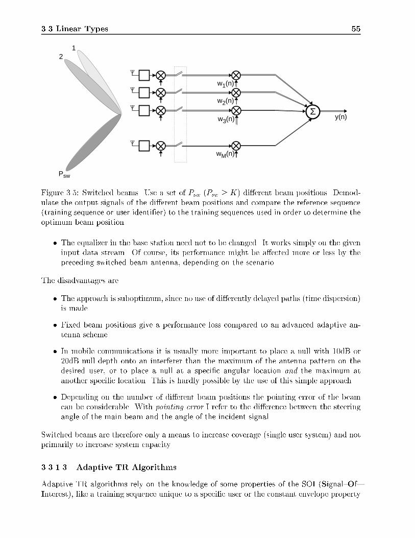
3.3 Linear Types 55
Σ
12
Psw
w1(n)
w3(n)
wM(n)
w2(n)
y(n)
Figure 3.5: Switched beams. Use a set of Psw (Psw � K) di�erent beam positions. Demod-ulate the output signals of the di�erent beam positions and compare the reference sequence(training sequence or user identi�er) to the training sequences used in order to determine theoptimum beam position.
� The equalizer in the base station need not to be changed. It works simply on the giveninput data stream. Of course, its performance might be a�ected more or less by thepreceding switched beam antenna, depending on the scenario.
The disadvantages are
� The approach is suboptimum, since no use of di�erently delayed paths (time dispersion)is made.
� Fixed beam positions give a performance loss compared to an advanced adaptive an-tenna scheme.
� In mobile communications it is usually more important to place a null with 10dB or20dB null depth onto an interferer than the maximum of the antenna pattern on thedesired user, or to place a null at a speci�c angular location and the maximum atanother speci�c location. This is hardly possible by the use of this simple approach.
� Depending on the number of di�erent beam positions the pointing error of the beamcan be considerable. With pointing error I refer to the di�erence between the steeringangle of the main beam and the angle of the incident signal.
Switched beams are therefore only a means to increase coverage (single user system) and notprimarily to increase system capacity.
3.3.1.3 Adaptive TR Algorithms
Adaptive TR algorithms rely on the knowledge of some properties of the SOI (Signal{Of{Interest), like a training sequence unique to a speci�c user or the constant envelope property
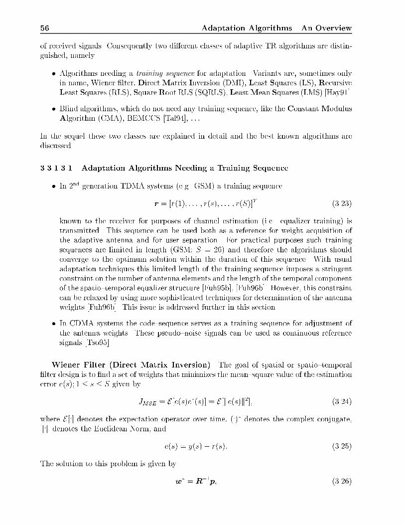
56 Adaptation Algorithms|An Overview
of received signals. Consequently two di�erent classes of adaptive TR algorithms are distin-guished, namely
� Algorithms needing a training sequence for adaptation. Variants are, sometimes onlyin name, Wiener �lter, DirectMatrix Inversion (DMI), Least Squares (LS), RecursiveLeast Squares (RLS), SquareRoot RLS (SQRLS), LeastMean Squares (LMS) [Hay91].
� Blind algorithms, which do not need any training sequence, like the ConstantModulusAlgorithm (CMA), BEMCCS [Tal94], : : :
In the sequel these two classes are explained in detail and the best known algorithms arediscussed.
3.3.1.3.1 Adaptation Algorithms Needing a Training Sequence
� In 2nd generation TDMA systems (e.g. GSM) a training sequence
r = [r(1); : : : ; r(s); : : : ; r(S)]T (3.23)
known to the receiver for purposes of channel estimation (i.e. equalizer training) istransmitted. This sequence can be used both as a reference for weight acquisition ofthe adaptive antenna and for user separation. For practical purposes such trainingsequences are limited in length (GSM: S = 26) and therefore the algorithms shouldconverge to the optimum solution within the duration of this sequence. With usualadaptation techniques this limited length of the training sequence imposes a stringentconstraint on the number of antenna elements and the length of the temporal componentof the spatio{temporal equalizer structure [Fuh95b], [Fuh96b]. However, this constraintcan be relaxed by using more sophisticated techniques for determination of the antennaweights [Fuh96b]. This issue is addressed further in this section.
� In CDMA systems the code{sequence serves as a training sequence for adjustment ofthe antenna weights. These pseudo{noise signals can be used as continuous referencesignals [Tso95].
Wiener Filter (Direct Matrix Inversion) The goal of spatial or spatio{temporal�lter design is to �nd a set of weights that minimizes the mean{square value of the estimationerror e(s); 1 � s � S given by
JMSE = E [e(s)e�(s)] = E [ke(s)k2]; (3.24)
where E [:] denotes the expectation operator over time, (:)� denotes the complex conjugate,k:k denotes the Euclidean Norm, and
e(s) = y(s)� r(s): (3.25)
The solution to this problem is given by
w� = R�1p; (3.26)

3.3 Linear Types 57
where R is the MRt �MRt correlation matrix of the antenna output
R = Es[x(s)xH(s)] = lim
s!1
1
S
SXs=1
x(s)xH(s)
!; (3.27)
and p is the MRt � 1 cross{correlation vector between the antenna output and the desiredresponse r(s)
p = Es[x(s)r�(s)] = lim
s!1
1
S
SXs=1
x(s)r�(s)
!: (3.28)
Note that this de�nition of the Wiener �lter is a generalization of the conventional time{domain (M = 1; Rt > 1) Wiener �lter [Hay91] to the time{space domain (M > 1; Rt > 1) orthe space domain only (M > 1; Rt = 1).
If the correlation matrix R and the cross{correlation vector p are replaced by their esti-mates from a �nite length noisy sequence (S <1), R and p, respectively, one uses the termDMI or SMI solution to address this di�erence.
Least Squares The goal of least squares is to minimize the cost function
"LS =SXs=1
ky(s)� r(s)k2: (3.29)
The problem can be stated in the form
Bw = r; (3.30)
where B is the direct{data matrix containing the samples of the array output during thetraining sequence
B = [x(1);x(2); : : : ;x(S)]T : (3.31)
The optimum solution (in the least squares sense) is given by
w = B+r; (3.32)
where (:)+ denotes the Moore{Penrose pseudoinverse [Gol83].
This method can be viewed as the deterministic counterpart to Wiener �lter theory[Hay91]. Note that B and R are related by
R =1
SBHB: (3.33)
The reason for using the word deterministic is that for the derivation of the optimum LSsolution to the optimization problem in Equation (3.30) no assumptions about the statisticalproperties of the involved quantities have been made. In contrast, for the Wiener �lter thereis an expectation operator at the beginning (Equation (3.24)), therefore statistics are involvedin its derivation.

58 Adaptation Algorithms|An Overview
Recursive Least Squares (RLS) Algorithm The RLS algorithm is a recursive im-plementation of the least squares algorithm. The performance index to be minimized is
"RLS =SXs=1
�S�sky(s)� r(s)k2; (3.34)
where � is a positive constant (0 < � � 1). The inverse of 1 � � is, roughly speaking, ameasure of the memory of the algorithm | � is therefore also named the "forgetting factor".This means that the algorithm can track, depending on the value of �, the changes of thechannel. A typical value for � is 0.95 for non{stationary channels. For the acquisition � = 1is best suited, i.e. the channel is assumed stationary during transmission of the trainingsequence.
The RLS algorithm can be summarized as follows [Hay91]:Initialization:
� = ��1RLSI; (3.35)
w(0) = 1; (3.36)
where � is the inverse of the cross{correlation matrix, �RLS is a small positive constant, I isthe (MRt �MRt) identity matrix, and 1 is the identity vector 1 = [1; 1; : : : ; 1]T with MRt
columns.
Adaptation:
k(s+ 1) =�(s)x(s+ 1)
� + xH(s+ 1)�(s)x(s+ 1); (3.37)
e(s+ 1) = r(s+ 1)�wH(s)x(s+ 1); (3.38)
w�(s+ 1) = w�(s) + k(s+ 1)e�(n); (3.39)
�(s+ 1) =1
�(�(s)� k(s+ 1)xH(s)�(s)); (3.40)
where e(s) is the a priori estimation error and k(s) is referred as the gain vector.
The computational cost of the RLS algorithm may be reduced by de�ning
l(s+ 1) =1
��(s)x(s+ 1): (3.41)
Equations (3.37) and (3.40) can now be rewritten as
k(s+ 1) = [1 + xH(s+ 1)l(s + 1)]�1l(s+ 1) (3.42)
and
�(s+ 1) =1
�(�(s)� k(s+ 1)lH(s+ 1)): (3.43)

3.3 Linear Types 59
Square{Root RLS Algorithm Most of the operations for the RLS{algorithm involvethe computation of �(s). This part of the computation is also susceptible to roundo� noise.To remedy that problem, algorithms have been developed, which avoid the computation of�(s). Instead, they are based on a decomposition of �(s) in the form
�(s) = S(s)D(s)ST (s); (3.44)
where S(s) is a lower triangular matrix and D(s) is a diagonal matrix. This decompositionis called a Cholesky factorization or a square{root factorization [Bie77].
Square{root algorithms neither calculate nor update �(s). Instead, the time updating isperformed on S(s) and D(s).
The algorithm can be summarized as follows [Hsu82]:Initialization:
d(0) = [d1; d2; : : : ; dm; : : : ; dM ]T = 1; (3.45)
�li = 0; l = 1; 2; : : : ;M ; i = l + 1; l + 2; : : : ;M; (3.46)
w(0) = 1; (3.47)
where dm are the elements of the diagonal matrix D(s) and �li are the elements of the lowertriangular matrix S(s).
Adaptation:
"(s) = r(s)�wH(s� 1)x(s) (3.48)
f1 = x�1(s); (3.49)
fi =i�1Xl=1
�lix�l (s) + x�i (s) i = 2; : : : ;M; (3.50)
g = d(s� 1) f ; (3.51)
�1 = � + g1f�1 ; (3.52)
�i = �i�1 + gif�i ; i = 2; : : : ;M; (3.53)
hq = 1 + q; (3.54)
ht = �Nq; (3.55)

60 Adaptation Algorithms|An Overview
=1
�1 + ht; (3.56)
d1(s) = d1(s� 1)hq(� + ht) ; (3.57)
� = �i�1 + ht; (3.58)
�i = �fi ; (3.59)
=1
�i + ht; (3.60)
di(s) = di(s� 1)hq� ; (3.61)
�1 = �li; (3.62)
�li = �1 + g�l �i; (3.63)
gl = gl + gi��1 ; (3.64)
e(s) = "(s) ; (3.65)
w�(s) = w�(s� 1) + ge; (3.66)
where denotes elementwise vector multiplication and � and q are adaptation coe�cients.They must be chosen as 0 < � � 1 and 0 � q < 1.
All constants, except �;M; ; hq; q; di;�i; i = 1; 2; : : : ;M; are complex quantities. Thequantities de�ned in Eqn. (3.48) to Eqn. (3.57) are computed �rst. Equations (3.58) to(3.64) are evaluated recursively for i = 2; 3; : : : ;M and (3.62) to (3.64) are computed forl = 1; 2; : : : ; i� 1.
Fast RLS Algorithms Fast recursive least square algorithms as proposed e.g. in[Cio84], [Car83], and [Ale84], exploit the shifting property of most sequential estimationproblems. This property utilizes the fact that at each iteration the number of new samplesentering and old samples leaving the adaptive structure is not MRt, but a smaller integerM .
For adaptive arrays the usefulness of this approach is limited to the wideband arrayscheme, i.e. where Rt > 1. Speeding up of the algorithm can be done in the time domainonly. Since data vectors of length M enter and leave the adaptation process, the computa-tional complexity of a fast RLS approach is of order O(M2Rt) instead of order O((MRt)
2),where O(:) means computational complexity in the order of (:). So it is not as computa-tional e�cient as the fast RLS algorithm for sequential estimation problems. Furthermoreits tendency to become numerically instable [Mue81] has to be investigated carefully.
However, as I will show in the following (Section 3.3.1.3.2), there is no cogent reasonto use fast RLS{type algorithms for wideband arrays since much simpler, stable, inherentlyparallel, and even computationally cheaper techniques can be applied to the task of weightdetermination.

3.3 Linear Types 61
Least{Mean{Squares (LMS) Algorithm The LMS algorithm is based on instanta-neous gradient error estimates. The algorithm can be summarized as follows [Hay91]:Initialization:
w(0) = 1 (3.67)
Adaptation:
e(s) = r(s)� y(s) = r(s)�wH(s)x(s); (3.68)
w�(s+ 1) = w�(s) + �x(s)e�(s); (3.69)
where e(s) is the di�erence between the desired and the actual array output (the error), and� (0 < � < 1) is the step size parameter a�ecting the convergence behavior of the algorithm.
Convergence Speed of Adaptation Algorithms I compare the convergence speed ofthe di�erent adaptation algorithms for one typical scenario. The number of antenna elementsis set toM = 5 with a spacing of d=� = 0:5. Two equipowered signals s1(�); s2(�) are incidentat the array with '1 = 0� and '2 = 45� measured from array broadside, where the secondwavefront is a delayed version of the �rst. The SNR (Signal{to{Noise Ratio) of both signalsis set to 20dB (SNR = kskk2=(2�2) = 20dB; k = 1; 2). The transmission protocol was chosenaccording to the GSM{standard [Gsm90]. The parameters for the algorithms are
� LMS: The step size parameter � of the LMS was set to � = �max=2, with the maximumstepsize �max given by [Hay91]
�max =2
�1; (3.70)
where � = diagf�mgMm=1 is the diagonal matrix containing the ordered eigenvalues �m(i.e. �1 � �2 � : : : � �m � : : : � �M) of the estimate of the covariance matrix
R =1
S
SXs=1
x(s)xH(s): (3.71)
� RLS (SQRLS): For the RLS the parameters are � = 1 and �RLS = 10�9. For theSQRLS the parameters are � = 10�4 and q = 1.
The performance of the adaptation algorithms in terms of settling time and output SNIRare given in Figure 3.6. I de�ne the settling time of the corresponding algorithm as theamount of time which is necessary to decrease the MSE (Mean Squared Error) kek2 forthe LMS algorithm (the innovation kek2 for the RLS and SQRLS algorithms) within thetraining sequence below 10�3. Note that theoretically the MSE should be in the mean aslow as MSEmin = 2:5:10�6. The larger value of MSE = 10�3 was chosen in order to ensureconvergence of the algorithms for all situations, since the actual noise contribution withinthe training sequence might be well above the mean value in some situations. Since theiterative algorithms are possibly not convergent within a single training sequence, I used thesame training sequence repeatedly until kek2 < 10�3. Figure 3.6a shows the settling time
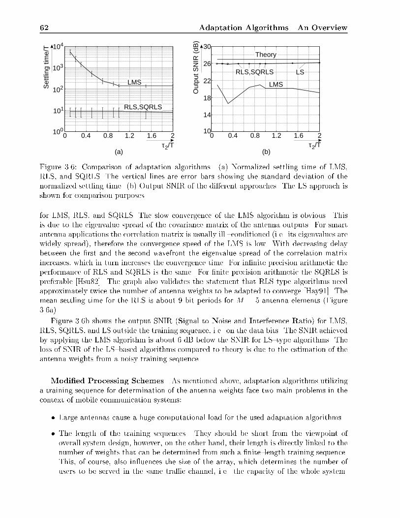
62 Adaptation Algorithms|An Overview
LMS
LS
LMS
RLS,SQRLS
RLS,SQRLS
Theory
0 00.4 0.40.8 0.81.2 1.21.6 1.62 2100
101
102
104
103
10
14
18
22
26
30
τ2/T τ2/T
Set
tling
tim
e/T
Out
put S
NIR
(dB
)
(a) (b)
Figure 3.6: Comparison of adaptation algorithms. (a) Normalized settling time of LMS,RLS, and SQRLS. The vertical lines are error bars showing the standard deviation of thenormalized settling time. (b) Output SNIR of the di�erent approaches. The LS approach isshown for comparison purposes.
for LMS, RLS, and SQRLS. The slow convergence of the LMS algorithm is obvious. Thisis due to the eigenvalue spread of the covariance matrix of the antenna outputs. For smartantenna applications the correlation matrix is usually ill {conditioned (i.e. its eigenvalues arewidely spread), therefore the convergence speed of the LMS is low. With decreasing delaybetween the �rst and the second wavefront the eigenvalue spread of the correlation matrixincreases, which in turn increases the convergence time. For in�nite precision arithmetic theperformance of RLS and SQRLS is the same. For �nite precision arithmetic the SQRLS ispreferable [Hsu82]. The graph also validates the statement that RLS type algorithms needapproximately twice the number of antenna weights to be adapted to converge [Hay91]. Themean settling time for the RLS is about 9 bit periods for M = 5 antenna elements (Figure3.6a).
Figure 3.6b shows the output SNIR (Signal to Noise and Interference Ratio) for LMS,RLS, SQRLS, and LS outside the training sequence, i.e. on the data bits. The SNIR achievedby applying the LMS algorithm is about 6 dB below the SNIR for LS{type algorithms. Theloss of SNIR of the LS{based algorithms compared to theory is due to the estimation of theantenna weights from a noisy training sequence.
Modi�ed Processing Schemes As mentioned above, adaptation algorithms utilizinga training sequence for determination of the antenna weights face two main problems in thecontext of mobile communication systems:
� Large antennas cause a huge computational load for the used adaptation algorithms.
� The length of the training sequences. They should be short from the viewpoint ofoverall system design, however, on the other hand, their length is directly linked to thenumber of weights that can be determined from such a �nite{length training sequence.This, of course, also in uences the size of the array, which determines the number ofusers to be served in the same tra�c channel, i.e. the capacity of the whole system.

3.3 Linear Types 63
In general, the larger the antenna, the better the Signal{to{Noise Ratio (SNR), theSignal{to{Interference Ratio (SIR) and correspondingly the lower the Bit{Error{Rate(BER) at its output and the larger the system capacity.
This section introduces an algorithmic scheme for wideband arrays, which is inherently par-allel and therefore needs no fast RLS structures, and, on the other side, requires less trainingbits than conventional adaptation schemes. As already mentioned, the length of the trainingsequence imposes a stringent constraint on the number of meaningful determinable antennaweights [Fuh95b]. As a rule of thumb, only S=2 coe�cients can be meaningfully determinedfrom an S{bit training sequence (MRt � S=2) [Fuh95b]. This section introduces some ap-proaches to determine a number of antenna weights that exceeds the length of the trainingsequence. Actually, I will show that the number of array elements, M , is bounded by thelength of the training sequence, whereas the length of the tapped delay lines, Rt, for thewideband scheme is unbounded.
The computational complexity of the common approach for adjusting the antenna weightswith DMI is in the order ofOf(MRt)
3g. The two algorithmic schemes introduced in the sequelwill have computational complexities of only OfM3Rtg and of only OfM3g, respectively.
3.3.1.3.2 Space{Time Decomposition (STD)
STD The essential idea behind this method is as follows (see also Figure 3.4):
If we adjust the weights of each temporal stage wr; 1 � r � Rt of a wideband array inde-pendently and do an MRC (Maximal Ratio Combining) of the output signals rather thanadjusting all weights at once, only the number of antenna elements M (but not the productof the number of antenna elements and the number of taps MRt) is constrained by the lengthof the training sequence S.
Return to the wideband array of Figure 3.4. The weights of the �rst temporal stagew1 = [w11; w21; : : : ; wM1]
T are adjusted in such a way as to optimally receive a version ofthe desired signal with the corresponding delay to the reference time (for the �rst stage thedelay is equal to (Rt � 1)T ) and to null out any other contribution. Likewise, the weightsof the following Rt � 1 stages wr = [w1r; w2r; : : : ; wMr]
T , 2 � r � Rt, are adjusted in orderto optimally receive the desired signal with the corresponding delay (if there is any). Theoutput signals of these stages are combined to yield the sum output y(n). If the array is ableto spatially resolve delayed paths it steers di�erent antenna patterns in di�erent directionsat di�erent delays.
As explained above, instead of determining the whole weight vector at once, we now breakup the large optimization problem (see Eqn. 3.30) into a set of Rt smaller, independentoptimization problems
Brwr = r; 1 � r � Rt; (3.72)
where the matrix Br follows as
Br = [xr(1);xr(2); : : : ;xr(S)]T (3.73)
with xr(s) being the input signal of the r{th stage given by
xr(s) = [x1(s� r + 1); x2(s� r + 1); : : : ; xM(s� r + 1)]T : (3.74)
64 Adaptation Algorithms|An Overview
That is, optimization is done for each stage separately, and, if desired, in parallel. The outputsignals yr(n) = w
Tr xr(n) and xr(n) = xr�1(n�1) for 2 � r � Rt, have to be combined to one
single output y(n). The optimum combining strategy is MRC, i.e. the signals are weightedproportional to their individual SNRs (Signal{to{Noise Ratios) and then summed [Oga92]
y(n) =pSNRTyRt(n); (3.75)
where SNR = [SNR1; SNR2; : : : ; SNRRt]T denotes the vector containing the SNRs, and
yRt(n) = [y1(n); y2(n); : : : ; yRt(n)]T is the vector of the outputs of the di�erent stages. The
SNR of the r{th stage is derived from
SNRr =
r
r �Brwr
2
: (3.76)
STD requires only OfM3Rtg operations for weight adjustment. The adaptation of di�erentstages can be done in parallel, which speeds up computation.
In principle, in�nitely many tapped delay line elements can be inserted without a�ectingthe length of the required training sequence.
STD{SIMI The STD approach can even be re�ned a second time.Only one M �M correlation matrix has to be inverted to determine all weight vectors.
Consider the matrices Br; 1 � r � Rt in Equation (3.72). They are given by
Br = [x(Rt + 1� r);x(Rt + 1� r + 1); : : : ;x(Rt + 1� r + S � 1)]T :(3.77)
Obviously, they have the S � Rt + 1 rows x(Rt);x(Rt + 1); : : : ;x(S) in common, but atdi�erent positions. If I take only these S � Rt + 1 rows and form a new common matrix
Bc = [x(Rt);x(Rt + 1); : : : ;x(S)]T ; (3.78)
I can formulate the new optimization problem as
Bcwr = rr; (3.79)
where
rr = r(r : S � Rt + r) (3.80)
is a shifted and truncated version of the training sequence. The solution of the system ofEquations (3.79) is now simply given by
wr = B+c rr; (3.81)
which requires only the inversion of one (M � M) matrix. Therefore the computationalcomplexity follows as OfM3g. I have constructed a modi�ed direct{data matrix Bc, whichconsists of only (S�Rt+1) samples of the array output instead of S samples, like the usualdirect{data matrices Br. This means that the number of antenna elements is bounded by

3.3 Linear Types 65
2 4 6 8 10 12 14 160
5
10
15
20
25
306
Output SNIR (dB)
-Number of antenna elements M
Input SNR
Figure 3.7: Output SNIR versus the number of antenna elements for the di�erent processingschemes for a length of the training sequence of S = 26 bits. |: Theory; o: LS adaptationwith noise{free training data; ��: ST;, �: STD{SIMI; �:�:: Conventional LS.
M � bS�Rt+12
c, where bxc denotes the nearest integer � x. This is in contrast to STD, wherethe number of antenna elements is bounded by S only.
I name this approach STD{SIMI (STD SIngle Matrix Inversion).
The number Rt of temporal stages and their delays Tr can be determined from an impulseresponse estimate, as used in GSM [Mou92]. However, as I will show in Chapter 5, co{channelinterference severely impairs the quality of the impulse response estimates, especially inSDMA systems.
I will now demonstrate the superior performance of these new approaches with an ex-ample: Consider two equipowered signals with DOAs of 0� and 45� (measured from thearray broadside), delayed by one bit duration T , incident on a 1D{ULA. The input SNRof each signal be SNRin = 10 dB. The number of array elements M is taken as a vari-able, the spacing of the antenna elements be d = �=2, and the length of the tapped de-lay lines be Rt = 2. The transmission protocol is taken in accordance to the GSM stan-dard (S = 26). Figure 3.7 shows the output SNR, calculated from the data �elds of theGSM timeslot, versus the number of antenna elements M . The theoretical output SNIR isSNIRout = SNRout = SNRin + 10 log10M + 3dB, since there are two same{user same{powersignals incident. Two e�ects may be observed: (1) The conventional scheme, the STD, andthe STD{SIMI approach achieve their optimum performance when the length of the trainingsequence is twice the length of the weight vector to be determined. Since Rt = 2, this occursfor the STD approach at a value, which is twice (in general: Rt times) that of the conven-tional approach. (2) The STD and the STD{SIMI approach give higher output SNRs thanthe usual approach.
The degradation in output SNIR compared to theory comes from the estimation of the

66 Adaptation Algorithms|An Overview
2 4 6 8 10 12 14 160
5
10
15
20
25
306
Output SNIR (dB)
-Number of antenna elements M
Input SNR
Figure 3.8: Output SNIR versus the number of antenna elements for the di�erent processingschemes with oversampling. The oversampling factor C was set to C = 2. The trainingsequence was shortened to S = 13 bits. |: Theory; ��: STD; �:�:: Conventional LS.
weights from noisy data. This is con�rmed by the curve that shows the output SNR forestimation of the array coe�cients from the noise{free training data by the conventionalapproach. For M > 3 this curve �ts closely with theory. For M = 2 (3) it deviates fromtheory, since an array with two (three) elements has only one (two) degree(s) of freedom.Therefore it cannot simultaneously null out the interfering signal and put the maximum ontothe desired one (get the maximum antenna gain into the direction of the desired signal andsimultaneously null out the interference) for the simulated situation.
3.3.1.3.3 Oversampling If continuous phase modulated training sequences are utilized,e.g. GMSK (Gaussian Minimum Shift Keying), oversampling of this sequence provides ad-ditional information for the adaptation. Of course, the receiver has then to use oversampling,but that is no serious constraint since all commercially available receivers use this techniquealready.
Oversampling of the training sequence by a factor C theoretically increases the numberof weights that can be estimated from this sequence also by a factor C. Note, however,that only small oversampling factors can be used, since oversampling decreases the phasedi�erence between two samples and therefore decreases the distance of these samples insignal space. Additionally the noise contribution to two adjacent samples become more andmore correlated with increasing oversampling factors. This will further decrease estimationaccuracy.
Figure 3.8 shows the output SNIR for the same scenario as considered before. The over-sampling factor is C = 2, the noise is assumed to be ST{AWGN. The training sequencewas shortened to 13 bits. For this moderate oversampling factor the same performance is

3.3 Linear Types 67
0 5 10 15 200
5
10
15
20
25
30
35
406
Output SNIR (dB)
-Input SNR (dB)
Figure 3.9: Output SNIR versus the input SNR for iterative signal reconstruction. |:Theory; o: Adaptation with noise{free data; ��: LS adaptation.
achieved as for the conventional schemes, using only one sample per symbol.
3.3.1.3.4 Iterative Reference Signal Reconstruction The basic idea of iterative ref-erence signal reconstruction is to perform the whole optimization task repeatedly [Wel93]:
1. Calculate an antenna weight vector with maximum length (M1 � S=2) from the trainingsequence only. Set the other weights to zero, i.e. form an antenna with M1 elementsonly.
2. Apply the calculated weight vector of lengthM1 to the array signals and determine theoutput y(n).
3. Determine the nearest possible state of each output signal and reconstruct the complexenvelope of the ideal input sequence.
4. Use the whole timeslot of length N(� M) (or a part of it) as training sequence anddetermine the desired number of weights M .
Figure 3.9 shows the output SNIR for the same scenario as considered before, the number ofantenna elements was set toM = 16 and the training sequence was shortened to 8 bits. Onlyone of the incoming paths is resolved, the second one is regarded as interference, i.e. Rt = 1.At the �rst iteration M1 = 4 antenna coe�cients have been determined, at the second stepthe number of determined coe�cients was set to M = 16. This procedure gives noticeableproblems for SNR < 10dB. An intermediate step with M2 = 8 weights was introduced, i.e.the number of weights to be estimated was gradually increased, but the results show nodi�erence to that obtained without applying an intermediate step.

68 Adaptation Algorithms|An Overview
Only for SNR> 8dB the full array gain was achieved. For input SNRs smaller than 8dBthe output SNIR degrades strongly. For an input SNR<4dB the system provides even lessoutput SNIR than the input SNR is (although there are M = 16 antenna elements), i.e. thesignals could not be resolved.
3.3.1.3.5 Blind Adaptation Algorithms (CMA) Blind algorithms do not need anytraining sequence. The desired signal constellation is recovered by using other informationof the received signal. This can be the size of the symbol alphabet or the constant enve-lope property of the signal (CMA [Tre83]). Since many mobile communication systems useconstant envelope signals (MSK, GMSK) this leads directly to the application of the CMAalgorithm. No training sequence is used for the CMA, therefore user separation is impossiblewith the CMA algorithm alone. For separation of two or more users (or, equivalently, toensure capture of the wanted signal) a signal cancellation scheme has to be used in additionto the CMA [Shy94].
CMA CMA tries to minimize the cost function
JCMA = Ef[ky(n)kpCMA � �pCMA
CMA ]qCMAg; (3.82)
where �CMA is the input constant modulus and pCMA and qCMA are integers. I choose herethe "2{2"{version of CMA (pCMA = qCMA = 2) and � = 1. The weight initialization is givenby
w(0) = 1: (3.83)
The weight update equation for steepest descent CMA is
w(n+ 1) = w(n)� 2�CMAx(n)�y(n)sign(ky(n)k2 � 1); (3.84)
where
sign(x) =
�1 : x � 00 : elsewhere
(3.85)
is the signum{function and n can vary, in contrast to non{blind algorithms, over the wholelength N of the timeslot.
Note the apparent similarity of this equation to the updating equation (Equation (3.69))of the LMS{algorithm. It shows that CMA is essentially a stochastic gradient descent al-gorithm, analogous to the LMS{algorithm, but uses a performance measure distinct frommean{squared error [Tre83].
Further results concerning CMA for spatial and spatio{temporal equalization are givenin [May94], [May93], [Ohg93], and [Kik94].
Signal Canceller For separation of two or more users (or, equivalently, to ensurecapture of the wanted signal) a signal cancellation scheme has to be applied in additionto the CMA [Shy94]. Figure 3.10 shows its principle. The signal canceller removes thecaptured source at the output, y(n), from the input x(n). Its adaptive weight vector is

3.3 Linear Types 69
w1(n)
u 3(d
)
u 2(d
)
u2(d+1)
w2(n+1)
u 1(d
)
u1(d+1)
w1(n+1)
y(n)
y(n)
u M(d
)
uM(d+1)
wM(n+1)
e1(d)x1(n+1)
τ=nT
x2(n+1)
x3(n+1)
xM(n+1)
e 1(d
)
x 1(n
)
e2(d)
e 2(d
)
x 2(n
)
e3(d)
eM(d)
e M(d
)
x M(n
)
w3(n)
w2(n)
wM(n)
Σ
+
+-
-
-
-+
+
LMS
CMA
CM Array
Adaptive Signal Canceller
Figure 3.10: CMA followed by a signal cancellation scheme. The signal canceller removesthe captured source at the output, y(n), from the input x(n). The error signal e(d) is equalto the output signal of the array after cancellation of the captured source and becomes theinput signal of the next stage.
u(d) = [u1(d); u2(d); : : : ; um(d); : : : ; uM(d)]T ; 1 � d � D, where D denotes an arbitrary
length of the input sequence (up to the whole timeslot, D = N). It is initialized byu(d) = [0; 0; : : : ; 0]T . These weights are updated e.g. by the use of the LMS{algorithmas
u(d+ 1) = u(d) + �LMSy�(d)e(d); (3.86)
where �LMS > 0 denotes the step size and e(d) is the error signal vector
e(d) = [e1(d); e2(d); : : : ; em(d); : : : ; eM(d)]T = x(d)� u(d)y(d): (3.87)
The error signal vector e(d) is equal to the output signal of the array after cancellation ofthe captured source and becomes the input signal of the next stage.
3.3.1.3.6 Pros and Cons of TR Algorithms The advantages of TR algorithms are:
� independent of the existence of DOAs,
� independent of the angular spread, as I will show in Chapter 5,
The disadvantages are:
� they do not determine DOAs directly, an information necessary for the downlink,
� synchronization has to be achieved before determination of the antenna weight vector,since one has to know the position of the training sequence for weight adaptation (except
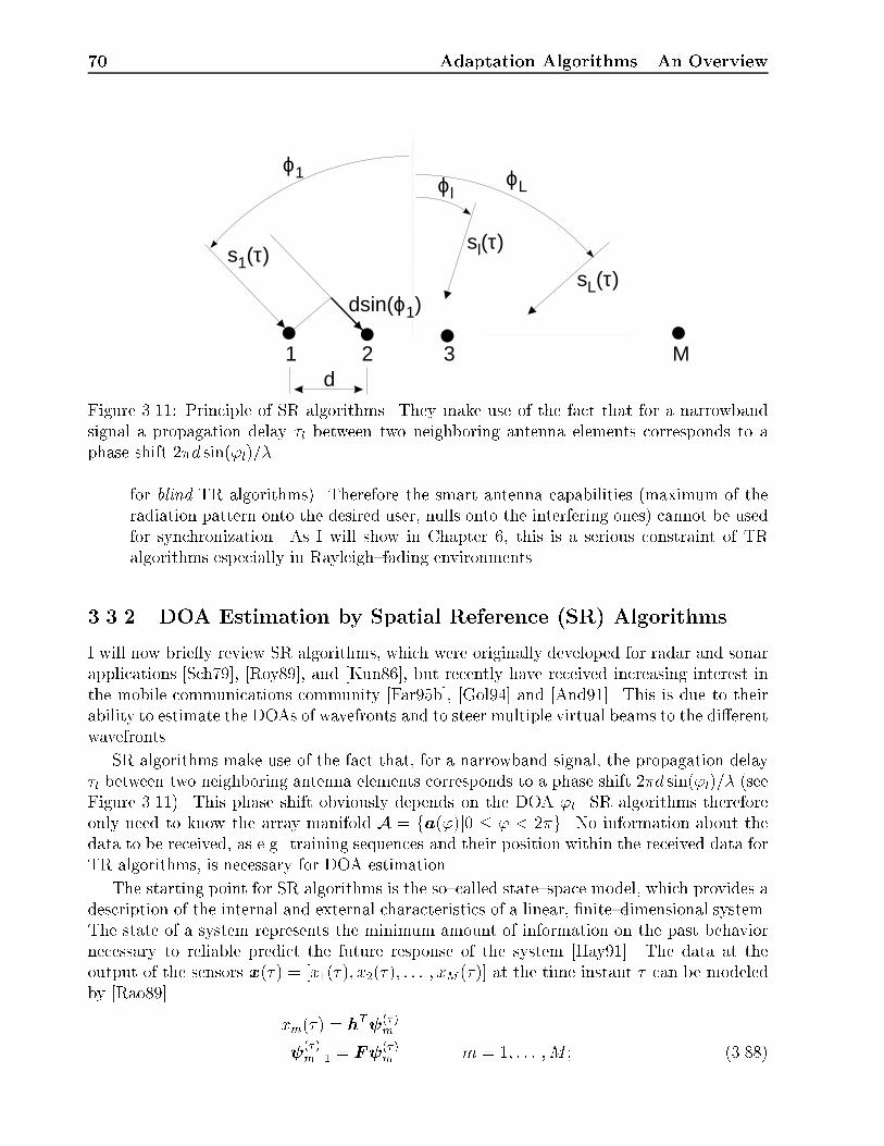
70 Adaptation Algorithms|An Overview
1 2 3 Md
ϕ1ϕl
ϕL
s1(τ)sl(τ)
sL(τ)dsin(ϕ1)
Figure 3.11: Principle of SR algorithms. They make use of the fact that for a narrowbandsignal a propagation delay �l between two neighboring antenna elements corresponds to aphase shift 2�d sin('l)=�.
for blind TR algorithms). Therefore the smart antenna capabilities (maximum of theradiation pattern onto the desired user, nulls onto the interfering ones) cannot be usedfor synchronization. As I will show in Chapter 6, this is a serious constraint of TRalgorithms especially in Rayleigh{fading environments.
3.3.2 DOA Estimation by Spatial Reference (SR) Algorithms
I will now brie y review SR algorithms, which were originally developed for radar and sonarapplications [Sch79], [Roy89], and [Kun86], but recently have received increasing interest inthe mobile communications community [Far95b], [Gol94] and [And91]. This is due to theirability to estimate the DOAs of wavefronts and to steer multiple virtual beams to the di�erentwavefronts.
SR algorithms make use of the fact that, for a narrowband signal, the propagation delay�l between two neighboring antenna elements corresponds to a phase shift 2�d sin('l)=� (seeFigure 3.11). This phase shift obviously depends on the DOA 'l. SR algorithms thereforeonly need to know the array manifold A = fa(')j0 � ' < 2�g. No information about thedata to be received, as e.g. training sequences and their position within the received data forTR algorithms, is necessary for DOA estimation.
The starting point for SR algorithms is the so{called state{space model, which provides adescription of the internal and external characteristics of a linear, �nite{dimensional system.The state of a system represents the minimum amount of information on the past behaviornecessary to reliable predict the future response of the system [Hay91]. The data at theoutput of the sensors x(�) = [x1(�); x2(�); : : : ; xM(�)] at the time instant � can be modeledby [Rao89]
xm(�) = hT (�)
m
(�)m+1 = F
(�)m m = 1; : : : ;M ; (3.88)
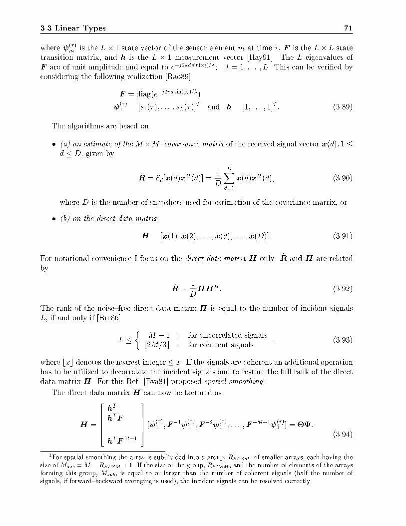
3.3 Linear Types 71
where (�)m is the L� 1 state vector of the sensor element m at time � , F is the L� L state
transition matrix, and h is the L � 1 measurement vector [Hay91]. The L eigenvalues ofF are of unit amplitude and equal to e�j2�d sin('l)=�; l = 1; : : : ; L. This can be veri�ed byconsidering the following realization [Rao89]
F = diag(e�j2�d sin('l)=�)
(�)1 = [s1(�); : : : ; sL(�)]
T and h = [1; : : : ; 1]T : (3.89)
The algorithms are based on
� (a) an estimate of the M�M{covariance matrix of the received signal vector x(d); 1 �d � D, given by
R = Ed[x(d)xH(d)] = 1
D
DXd=1
x(d)xH(d); (3.90)
where D is the number of snapshots used for estimation of the covariance matrix, or
� (b) on the direct data matrix
H = [x(1);x(2); : : : ;x(d); : : : ;x(D)]: (3.91)
For notational convenience I focus on the direct data matrix H only. R and H are relatedby
R =1
DHHH : (3.92)
The rank of the noise{free direct data matrix H is equal to the number of incident signalsL, if and only if [Bre86]
L ��
M � 1 : for uncorrelated signalsb2M=3c : for coherent signals
; (3.93)
where bxc denotes the nearest integer � x. If the signals are coherent an additional operationhas to be utilized to decorrelate the incident signals and to restore the full rank of the directdata matrix H. For this Ref. [Eva81] proposed spatial smoothing1.
The direct data matrix H can now be factored as
H =
26664hT
hTF...hTFM�1
37775 [ (�)
1 ;F�1 (�)1 ;F�2 (�)
1 ; : : : ;F�M+1 (�)1 ] = �:
(3.94)
1For spatial smoothing the array is subdivided into a group, RSPSM , of smaller arrays, each having thesize of Msub =M �RSPSM + 1. If the size of the group, RSPSM , and the number of elements of the arraysforming this group, Msub, is equal to or larger than the number of coherent signals (half the number ofsignals, if forward{backward averaging is used), the incident signals can be resolved correctly.

72 Adaptation Algorithms|An Overview
To determine � and we compute an SVD (Singular Value Decomposition) of H as
H = [ U 1 U 2 ]
��1 00 0
� �V H
1
V H2
�; (3.95)
where the columns of U and V are the left and right singular vectors ofH, respectively. Thediagonal matrix �1 contains the L singular values. The space spanned by the eigenvectorsin U 1 belonging to the non{zero eigenvalues of H is the signal subspace.
The matrix � is chosen as
� = U 1�1=21 (TAM) (3.96)
or
� = U 1 (ESPRIT); (3.97)
where TAM stands for Toeplitz Approximation Method [Kun86] and ESPRIT stands forEstimation of Signal Parameters via Rotational Invariance Techniques [Roy89]. Once �and are chosen, F is uniquely de�ned. It can be determined from � since it satis�es thefollowing linear system of equations
�#F = �"; (3.98)
where
�# =
26664h
hF...hF L�1
37775 and �" =
26664hF
hF 2
...hF L
37775 ; (3.99)
are shifted versions of �. This results in
F = (�#)�1�": (3.100)
In the presence of noise the matrixH has full rank with probability one. Therefore I calculatethe SVD of the noisy data matrix H as
H = [ U 1 U 2 ]
��1 0
0 �2
�"V
H
1
VH
2
#; (3.101)
where the diagonal matrix �1 contains the L dominant singular values. The space spannedby the eigenvectors in U 2 belonging to the (M � L) non{dominant eigenvalues of H is thenoise subspace.
Since L is not known in advance, it has to be estimated from the available data. Thenumber of incident sources L (i.e. the dimension of the signal subspace), which is an infor-mation necessary for the algorithm, can be determined by the model{theoretic criteria fromRef. [Xu94] or [Wax85]. The criteria named AIC (An Information Criterion) [Aka74] andMDL (Minimum Description Length) [Scw78] are given by
AIC(L) = W (L) + pf(L);
MDL(L) = W (L) +1
2pf(L)ln(D); (3.102)

3.3 Linear Types 73
where L is the estimated number of sources, ln(:) denotes the natural logarithm, and pf (L)
denotes the free (adjustable) parameters in the estimate of the covariance matrix R, assumingthat there are L sources. The minimizers of the AIC and MDL criteria are chosen as theAIC and MDL estimates of L [Wax85].
The statistic W (L) follows as
W (L) = �D(M � L)ln
8>>>>><>>>>>:
MQ
l=L+1
�l
!1=(M�L)
1M�L
MPl=L+1
�l
9>>>>>=>>>>>;; (3.103)
where �l are the eigenvalues of R and pf (L)is given by
pf(L) =1
2L(2M � L + 1): (3.104)
An alternative criterion is the RoE (Ratios of Eigenvalues) criterion. Let us de�ne a set
R� = fr�;1; r�;2; : : : ; r�;M�1g (3.105)
with
r�;m =�m � �m+1
�m+1: (3.106)
The estimated number of incident sources follows now from
LRoE = maxmfR�g = max
mfr�;1; r�;2; : : : ; r�;M�1g: (3.107)
Let the matrices �1, �2 be �1 = diag(�1; : : : ; �L) and �2 = diag(�L+1; : : : ; �M). Now, � isgiven by
� = U 1(�s
1)1=2 (TAM); (3.108)
or
� = U 1 (ESPRIT); (3.109)
where
�s
1 = diag(�s1; : : : ; �sL) and �sl = �l � �2n; (3.110)
where �2n is the estimated variance (power) of the noise, given by
�2n =1
M � L
MXl=L+1
�l: (3.111)
Then
F = (�#)�1�
": (3.112)

74 Adaptation Algorithms|An Overview
Afterwards an eigendecomposition of F is performed, i.e.
F = C�C�1: (3.113)
The diagonal matrix � is an approximation for
� = diag(e�j2�d sin('1)=�; e�j2�d sin('2)=�; : : : ; e�j2�d sin('L)=�): (3.114)
Therefore the DOAs can be determined from the diagonal elements of � = diag(�1; : : : ; �L)via
'l = arcsin
�Im(ln(�l))�
2�d
!: (3.115)
Using the matrix � we can construct an estimate of the so{called array steering matrix
A = [a('1); : : : ; a('L)]; (3.116)
where
a('k) = [1; e�j2�d sin('l)=�; : : : ; e�j2�(M�1)d sin('l)=�]T (3.117)
is the array steering vector associated with direction 'l. For estimation of the signal wave-fronts I use a linear estimator [Ali94] s(�) = Wx(�) such that the Frobenius norm of theerror kx(�)� As(�)kF is minimized. This can be achieved by choosing
W =
26664wH
1
wH2...wHL
37775 = A
+; (3.118)
which is the pseudoinverse of A [Gol83].
The l{th row of the estimated weighting matrixW , wHl , can be interpreted as the array
weight vector providing the reconstruction of the l{th wavefront and steering nulls in thedirections of the other L� 1 incident wavefronts.
A straightforward method to increase the resolution capability of SR algorithms for point{symmetrical arrays is forward{backward averaging [Eva81], [Pil86]. Instead of using theconventional covariance matrix R (direct data matrix H) the forward{backward averagedcovariance matrix
Rfb =1
2(R + Rb); (3.119)
is employed. Here
Rb = Ed[x(b)(d)x(b)H(d)] = 1
D
DXd=1
x(b)(d)x(b);H(d) (3.120)

3.3 Linear Types 75
is the backward covariance matrix and x(b)(d) follows as
x(b)(d) = Ex�(d); (3.121)
which is simply a rearrangement of the complex conjugates of the array outputs. Thismeans, that the complex conjugate of the array output data vector at time � = dT , x�(d),is multiplied by the permutation matrix
E =
266640 0 : : : 0 10 0 : : : 1 0...
.... . .
......
1 0 : : : 0 0
37775 : (3.122)
This operation also enables resolution of (two) coherent signals. For more than two coherentsignals spatial smoothing [Eva81], [Pil86] has to be utilized.
Based on the forward{backward averaged covariance matrix Rfb a proposition for doingmost of the computations on real{valued matrix entries was recently presented in [Haa95].This algorithm is called 1D Unitary ESPRIT. An extension of 1D Unitary ESPRIT to twodimensions is given in [Zol96a]. With this algorithm it is possible to jointly estimate azimuth' and elevation # of the incident waves.
The principal ow diagram of SR algorithms is shown schematically in Figure 3.12.
Their advantages are:
� No training sequence is needed. Separation of users can be done by short user identi�ersor by correlation of the di�erent received signals.
� Di�erent paths carrying partial signals from a single user are separately resolved. Thisallows the application of optimum combining schemes.
� The delays of the di�erent paths can be determined.
� In contrast to TR algorithms, SR algorithms are insensitive to the chosen samplinginstant. However, to recover the data, the optimum sampling instant must be deter-mined. Of course, this step is much easier to perform for "clean" signals than for TRalgorithms, where synchronization has to be done before determination of the optimumweights.
� The estimated DOAs can be directly used for downlink beamforming.
The disadvantages are
� The array manifold has to be known in detail. This necessitates sophisticated calibra-tion algorithms to be applied before using SR algorithms. Gain and phase imbalancesbetween the RF hardware connected to each antenna element have to be calibratedout. The array has to be calibrated carefully | even during operation, since the envi-ronmental conditions are usually changing with the seasons.

76 Adaptation Algorithms|An Overview
Matrix Arrangement H
Singular ValueDecomposition
H=UΣV
Rank Determination of Σ
Determination of thestate transition matrix
Eigendecomposition of F
Determination of thesteering matrix A
Number ofSignals L
L
DOAs ϕ
ComplexEnvelopes s(τ)
Inputs Algorithmic Steps Outputs
x(d)
^
^
^
^^
^
Figure 3.12: Flow diagram of a DOA estimation algorithm.

3.3 Linear Types 77
� For usual mobile communication applications the number of incident signals exceedsthe number of signals resolvable by the algorithms. This drawback, which seems to beserious at the �rst glance, is addressed in the next example.
I will now illustrate this e�ect by an example. I consider the estimation accuracyof the complex{valued version of Unitary ESPRIT [Haa95] with spatial smooth-ing [Eva81] with M = 15 antenna elements with a subarray size of Msub = 8for spatial smoothing [Pil86], i.e. RSPSM = 7 coherent signals can be resolved.Further parameters are SNR = 10dB (for the signals to be resolved) and D = 50.1000 simulation runs were performed to ensure statistical stability of the results.Thirteen sinusoidal wavefronts are incident on the array, where seven out of them(the maximum resolution capability of the algorithm) are equipowered, with am-plitude sr, and angularly spaced by 20�. Only these seven signals can be resolvedby the algorithm. The six weaker | and therefore not resolved | signals withamplitude snr are located in between the seven stronger signals (see Figure 3.13a).The attenuation of the six weaker signals is de�ned by
Anr = �20 log�snrsr
�: (3.123)
Figure 3.13b shows the standard deviations of the DOAs of the resolved signalsversus the attenuation of the non{resolved signals. Figure 3.13c shows the out-put SNIR of the resolved signals. The algorithm is still capable of resolving theincident signals with largest power, even if the number of signals exceeds thetheoretically stated limit. Its performance degrades gracefully, as is evidenced bythe increasing standard deviations with increasing amplitudes of the non{resolvedsignals. The power di�erence between the resolved and the non{resolved signalshas to be at least 19dB for achieving an output SNIR for all incident signals equalto the input SNR.
� Computational load
� The incoming signals in a usual macrocell have both azimuth and elevation dependence.To resolve the directions properly a 2{dimensional (planar) array has to be utilized.This condition does not really pose a stringent constraint, since it was shown in [Egg94]and [Kel95] that the vertical angular spread could be neglected for most practical cases.A linear array therefore su�ces in most environments.
� Mutual coupling of the antenna elements. This means that the signal received by oneantenna element does not only depend on the incident signals but also on the signalson each other antenna element.

78 Adaptation Algorithms|An Overview
1 2 M
snr
sr
(a)
(b)
(c)
Sta
ndar
d D
evia
tion
(Deg
ree)
Attenuation of the Non-Resolved Waves (dB)
Attenuation of the Non-Resolved Waves (dB)
Out
put S
NIR
(dB
)
ϕ1=-60°
ϕ1 ϕ2
ϕ7
Theory
Input SNR
ϕ1=-60°
ϕ2=-40°
ϕ2=-40°
ϕ3=-20°
ϕ3=-20°
ϕ4=0°
ϕ4=0°
ϕ5=20°
ϕ5=20°
ϕ6=40°
ϕ6=40°
ϕ7=60°
ϕ7=60°
-10
0
10
20
30
5
5
10
10
15
15
20
20
25
25
30
30
35
35
40
400.01
0.1
1
10
Figure 3.13: Behavior of SR algorithms when the number of incident signals exceeds thenumber of maximum resolvable signals. (a) Investigated scenario, (b) Standard deviation ofthe estimated DOAs of the resolved signals. The curves for 'j and 'j+3, j = 1; 2; 3; overlap.(c) Output SNIR of the resolved signals. An attenuation of at least 19dB of the non{resolvedsignals is necessary so that the output SNIR of all resolved signals becomes at least equal tothe input SNR.

3.4 Nonlinear Antenna Types 79
Figure 3.14: E�ect of mutual coupling on the estimated DOA for VIASS.
To demonstrate the e�ect (and its remedy) I treat a 1D{ULA consisting of fourvertically stacked halfwave dipoles with a spacing of d = �=2. One plane waveis incident on the array. The array output currents were calculated using theNEC2{Code [Bur81]. Figure 3.14 shows the DOA calculated from the outputs ofNEC2 versus the actual DOA, the angle of the incident wavefront (SNR = 1).The used algorithm is VIASS [Fuh95a], a single{snapshot version of the complex{valued Unitary ESPRIT algorithm. The in uence of mutual coupling can beclearly seen. It depends on the DOA and has its maximum at ' = �45�. Fromthis maximum deviation I calculated a mutual coupling matrix by comparing theoutputs of the antenna array to the output of a single halfwave dipole consecutivelyput at each position of the array elements. After removal of the mutual couplinge�ect by means of this predetermined coupling matrix the inaccuracy of the DOA{estimation process is reduced considerably.
3.4 Nonlinear Antenna Types
Nonlinear antenna arrays have also been proposed recently: Decision Feedback Array (DFA)structures [Lin95] and Bayesian Arrays (BA) based on Radial Basis Function (RBF) neuralnetworks [Mun95], and vector channel multiuser MLSEs (Maximum Likelihood SequenceEstimator) [VaE76], [Ver86]. Both structures are well known from time{domain equaliza-tion problems [Che92], [DAr91] and have been shown to perform superior to their linearcounterparts.

80 Adaptation Algorithms|An Overview
T
T
Adaptationalgorithm
Trainingsequence
Output y(n)Weight
adaptation
++
+
-
-
+Slicer
Adaptationerror
Adaptationerror
TT T
TT T
T T T
T T T
+
w21(n)
x2(n)
w22(n)
w31(n)
x3(n)
w32(n)
wM1(n)
xM(n)
wM2(n) wM3(n)wMRt
(n)
wB1(n)wB(D1-1)(n)wBD1(n)
w3Rt(n)
w2Rt(n)
w1Rt(n)
w11(n)
x1(n)
w12(n) w13(n)
w23(n)
w33(n)
τ=nT
A
A
B
B
Feedforward filter
Feedback filter
Ant
enna
1
2
3
M
Trainingsequence
Figure 3.15: Decision feedback array. It consists of a feedforward �lter, a feedback �lter andthe slicer, which is the nonlinear element.
3.4.1 Decision Feedback Array (DFA)
A DFA basically consists of a feedforward �lter, a slicer (nonlinear element) and a feed-back �lter (Figure 3.15). Detected symbols are fed back to remove the postcursor ISI. Thefeedforward �lter cancels the precursor ISI.
Let
~x(n) = [xT (n); y(n� 1); y(n� 2); : : : ; y(n�D1)]T ; (3.124)
be the extended data vector, since it consists of the usual data vector and the fed backsymbols, and
~w(n) = [wT (n); wB1(n); wB2(n); : : : ; wBD1(n)]T ; (3.125)
the extended weight vector. The length of the feedback �lter is denoted by D1, it is deter-mined by the maximum excess delay of the channel. The vector x(n) denotes the usual data

3.4 Nonlinear Antenna Types 81
vector with the received signals at the antenna elements at the time instant � = nT andw(n) is the corresponding weight vector of the antenna elements. The array output is then
y(n) = ~w(n)T ~x(n): (3.126)
For weight adaptation let ~B be the extended direct{data matrix containing the samples ofthe array output and the symbols to be fed back during the span of the training sequence
~B = [~x(D1 + 1); ~x(D1 + 2); : : : ; ~x(S)]T : (3.127)
Note that during the training sequence the data vector ~x(s) is formed as
~x(s) = [xT (s); r(s� 1); r(s� 2); : : : ; r(s�D1)]T ; (3.128)
i.e. the known data symbols to be fed back are replaced by their ideal values from the trainingsequence.
For determination of the optimum weight vector in the least squares sense the system ofoverdetermined equations
~B ~w = ~r; (3.129)
with
~r = [r(D1 + 1); r(D1 + 2); : : : ; r(S)]T = r(D1 + 1 : S) (3.130)
has to be solved. It can be calculated via any one of the algorithms introduced in Section3.1.2.1.
Figure 3.16 shows the output SNIR versus the angular separation �' between two co{channel signals from the same user, which are delayed by one bit duration T . The numberof antenna elements was set to M = 8, their spacing is d=� = 0:5. The input SNR was set to10dB for each signal. The linear antenna types are sensitive to the angular separation of theincident signals, whereas the DFA is not. However, the output SNIR of the DFA structureis in general 5dB below the theoretical curve for linear processing and 3dB below the outputSNIR for STD for �' > 12�. For the considered situation, error propagation in the DFA(through the feedback �lter) is no critical issue. The DFA provides a gain against the lineararray structure only if the angle di�erence between the incident signals is less than �' = 6�.
3.4.2 Bayesian Arrays
RBF equalizers implement the optimum symbol detector according to Bayes law [DuH73]
P (�hjx) = px(xj�h)Php(x)
; (3.131)
where P (�hjx) is the a posteriori probability of class �h assuming the array output x,px(xj�h) is the conditional probability density function of x, Ph is the a priori probabil-ity of class �h, and p(x) is the probability density function of the array output vector x givenby
p(x) =
NmodXh=1
Php(xj�h); (3.132)

82 Adaptation Algorithms|An Overview
0 5 10 150
5
10
15
20
256
Output SNIR (dB)
-Angle di�erence �' (deg)
Input SNR
Figure 3.16: Output SNIR for the di�erent | linear and nonlinear | architectures. |:Theory; +: Theory for 1D{ULA; o: LS adaptation with noise{free training data; ��: STD;�:�:: Conventional LS; :::: DFA; �: DFA with ideal symbols fed back.
where Nmod denotes the number of possible symbols in the data to be transmitted (e.g. forMSK Nmod = 4). The RBF network basically consists of two layers: (1) The hidden layerand (2) the output layer (Figure 3.17).
The hidden layer is composed of Kh nodes, characterized by a vector c, the so{calledcenter. Each node is connected to each array output. The node calculates the weighteddistance between the input vector x and the center ch; 1 � h � Kh; as
z(h) = f(ch;x) = e� (x�ch)HR
�1n (x�ch)
�RBF ; (3.133)
where Rn is the noise correlation matrix, f(:) is the exponential function, and �RBF is thewidth of f(:). Note that for spatially and temporally uncorrelated noise, Rn is simply the(MRt�MRt){Identity matrix IMRt. This choice results in the optimum detector if the inputvectors x are disturbed by AWGN. Therefore a noise{whitening �lter prior to the applicationof the RBF network has to be implemented in the receiver. The transfer function Hw(j!) ofthe noise{whitening �lter is given by [Lee73]
Hw(j!) =1
HPB(j! + j!0)HBB(j!); (3.134)
where HPB(j! + j!0) is the transfer function of the passband �lter shifted to baseband,!0 = 2�f0 is the carrier angular frequency, and HBB(j!) is the transfer function of thebaseband �lter. The number of nodes, Kh, follows as
Kh =
�NKmod : narrowband array
NKLchannelmod : wideband array
; (3.135)

3.4 Nonlinear Antenna Types 83
Σ
-Learningalgorithm
τ=nTε1(n)
y(n)
Switch
Hidden layer
Noi
se w
hite
ning
filte
r
Inputlayer Linear combiner
Ant
enna
1
2
3
M
Trainingsequence
Radial basis function network
c1
c3
c2
cKh
w1 (n)(RBF)
w2 (n)(RBF)
w3 (n)(RBF)
wKh(n)(RBF)
Figure 3.17: Bayesian Arrays (BA) based on Radial Basis Function (RBF) neural networks.
where Lchannel is the memory of the channel normalized to a symbol duration T , i.e. thelength of the impulse response, the memory of the modulation process, and the �lters.
The centers of the neurons in the hidden layer are chosen from the S samples of thetraining sequence. Let Nh be the number of samples belonging to node class Kh during thetraining sequence, then
ch =1
Nh
NhXh=1
xh: (3.136)
Let z(n) be the output vector of the hidden layer,
z(n) = [z1(n); z2(n); : : : ; zKh(n)]T : (3.137)
The output layer linearly combines the outputs of the hidden layer to
y(n) = w(RBF )T (n)z(n): (3.138)
Let
Z = [z(1); z(2); : : : ; z(S)]T (3.139)
be the direct{data matrix of the outputs of the hidden layer during the training sequence.The optimum coe�cient vector w(RBF )(n) in a least{squares sense for the output layer is theone solving the overdetermined system of equations
Zw(RBF ) = r: (3.140)
Again, the solution can be calculated by the algorithms introduced before.
For a at fading channel both nonlinear schemes are theoretically equivalent to a linearadaptive array. On the one hand, as there is no time dispersion the feedback �lter of the DFAis useless. Only the spatial component remains. On the other hand, the decision regions forthe di�erent symbols can be separated by linear hypersurfaces. Therefore the RBF equalizerbecomes useless.

84 Adaptation Algorithms|An Overview
1
1
2 2
3
k
3
m
KM
+
+
+
+
+H(τ,t)
n1(τ)
hkm(τ,t)
n2(τ)
n3(τ)
nm(τ)
nM(τ)
Vector channel
Figure 3.18: Concept of a vector channel. The signals of K users sharing the same propa-gation medium, however, in general having di�erent channels, are received by M (spatiallyseparated) receivers.
3.4.3 Vector Channel Multiuser MLSE's and Antenna Arrays
The optimal receiver for the detection of signals in the presence of AWGN is well known tobe the ML (Maximum Likelihood) receiver [For72]. The concept of the scalar channel MLreceiver [For72] has been extended to vector channel transmission systems in [VaE76] and[Ver86], and to the joint detection of multiple signals in [Wal95].
Consider the system model depicted in Figure 3.18. There are K inputs (mobiles) to thevector channelH(�; t) and M outputs (antennas). The transmitted signal vector s(�) at thedelay instant � is
s(�) = [s1(�); s2(�); : : : ; sK(�)]T : (3.141)
The output signal follows as
x(�; t) = (HT � s)(�; t) + n(�); (3.142)
where � denotes elementwise convolution
xm(�; t) = (H(:; m)T � s)(�; t) + nm(�)
=KXk=1
(hkm � sk)(�; t) + nm(�) =KXk=1
1Z�1
hkm(�1 � �; t)s(�1) d�1: (3.143)
The optimum receiver consists of a bank of noise{whitening �lters, a bank of matched �lters,a bank of samplers, and a detector. The transfer function of the noise whitening �lter,Hw(j!), is given in Equation (3.134). The transfer function HMF (j!) of the combination ofmatched �lter and noise whitening �lter follows as
HMF (j!) =S�(j!)
HPB(j! + j!0)HBB(j!); (3.144)

3.4 Nonlinear Antenna Types 85
τ=nT
y1(n)
y2(n)y3(n)
yK(n)
Data Userk
Ant
enna
Rec
eive
rfr
onte
nd
Mat
ched
& n
oise
whi
teni
ng fi
lter
1
2
3
M
x1(n)
x2(n)
x3(n)
xM(n) Vec
tor
chan
nel
MLS
E
Channelestimator
Figure 3.19: Vector channel MLSE.
where S(j!) denotes the spectrum of the transmitted signal s(�). The denominator in thetransfer function of the matched �lter appears because the matched �lter has to take intoaccount the noise{whitening �lter. The outputs of the matched �lter form a su�cient statistic[LeM90] and are used for the optimum MLSE.
The single{sensor (M = 1) multiple{user MLSE was described in Reference [Wal95].There it was shown that the metric D2
n for the n{th step for jointly detecting K signals isgiven by
D2n = kx1(n)� xh(n)k2; (3.145)
with
xh(n) = H(:; 1)T (n) � dsh(n : n� Lchannel;k) (3.146)
denoting the hypothesis symbol. x1(n) denotes the received signal at � = nT , H(n) denotesthe (estimated) discrete{time impulse response, where the k{th element has a length ofLchannel;k, which is the memory of the k{th channel, sh(n : n � Lchannel;k) are the di�erentpossible sequences to be detected | the index (:)h stands for hypothesis, with the k{th columnhaving Lchannel;k elements. � d denotes discrete{valued convolution. To ease explanation, Iset Lchannel;k = Lchannel;i = Lchannel; 8k; i.
A metric for a multiple sensor (M > 1) single{user MLSE in conjunction with antennaarrays was described in [Bot95]. A combination of these two concepts leads to the multiple{sensor multiple{user adaptive array.
The discrete{time set of noise vectors fn(n)jn = 1; : : : ; Ng is a sequence of spatially andtemporally independent, zero{mean, white, complex Gaussian noise vectors. Therefore thelikelihood of a speci�c noise vector n(n) is given by [Wha71], [Bot95]
p(n(n)) =1
�MkRnke� 12nH(n)R
�1n n(n); (3.147)

86 Adaptation Algorithms|An Overview
where the noise correlation matrix is given by
Rn = Enfn(n)nH(n)g: (3.148)
Maximizing the likelihood of Equation (3.147) is equivalent to minimize the negative log{likelihood
L = �ln(p(n(n))) = [M ln(�) + ln(kRnk)� ln(2)] + nH(n)R�1n n(n):
(3.149)
The term in the square brackets is hypothesis{independent and can be dropped. The branchmetric follows therefore as [Bot95]
D2n = (x(n)� xh(n))HR�1
n (x(n)� xh(n)): (3.150)
Due to the assumptions about the noise process, the noise covariance matrix Rn follows as
Rn = �2IM ; (3.151)
where IM is the (M �M) identity matrix. Therefore I get for the branch metric
D2n = �2
MXm=1
kxm(n)� xm;h(n)k2; (3.152)
where � can be set to 1. This metric is the same as derived in Reference [VaE76] for thegeneral vector channel MLSE.
The Viterbi algorithm is an e�ective technique for minimization of Dn; 1 � n � N overall combinations of the transmitted sequences. In applying this algorithm the channel priorto noise addition is viewed as a �nite state Markov process. The states of this processrelate to data sequences of length Lchannel. The output of the channel can be described bya sequence of possible states. The task of the Viterbi algorithm is to �nd the most probablesequence of states. This is the data sequence having the smallest Euclidean distance betweenthe received signal and the receiver signal set. This sequence becomes the estimated datasequence [Wal95].
Figure 3.20 shows the basis for a single{channel MLSE for the optimal reception of MSK{modulated signals in an AWGN or at{fading channel. The Markov{diagram and the trellisdiagram consist of Nmod = 4 states.
The extension of the Viterbi algorithm to multiuser detection is straightforward. Myexplanation follows the one of [Wal95]. Assume that each state in the conventional demod-ulation/equalization process for User k at time n for a single signal is denoted by
�k(n) = (sn�1; sn�2; : : : ; sn�Lchannel); si 2 fs1; s2; : : : ; sNmodg: (3.153)
Now a superstate �k(n) can be formed by combining all these single state descriptors by
�k(n) = (�1(n); �2(n); : : : ; �K(n)): (3.154)
If there are NLchannel�1mod states for each signal, there are N
K(Lchannel�1)mod superstates. Since there
are in general ~Nmod transitions from each state, there are ~NKmod transitions from each super-
state. ~Nmod depends on the modulation format used, in general the equation ~Nmod = Nmod

3.4 Nonlinear Antenna Types 87
Re{sMSK(τ)}
Im{sMSK(τ)}
τ=0
τ=T
τ=T
bi=+1
bi=-1
11
1
n=1 n=2
12
2
2 23
3
3 3
44
4 4
(a) (b) (c)
Figure 3.20: Single{channel MLSE for optimal reception of MSK{modulated signals. (a)Phasor diagram. The phase changes by �90� within a bit duration, depending whether thetransmitted bit is bi = 1 or bi = �1. The possible states are numbered from 1 to 4. (b)Markov diagram for MSK. The arcs show the possible state changes. (c) Trellis diagram,showing the possible progression of the states over time.
holds. Exceptions are e.g. the (G)MSK modulation formats, where ~Nmod = Nmod=2. Sinceeach conventional state describes a �nite state Markov process, this property also appliesto the superstates. All principles known from the single{user Viterbi algorithm can now besimply applied to this problem and the optimal bit sequences can be detected, provided thatthe channel impulse responses for each path are known. Figures (3.21) and (3.22) show theMarkov diagram and the superstate trellis for a vector channel multiuser MLSE for MSKmodulated signals for K = 2 users. The exponential complexity increase compared to asingle{user MLSE is obvious from these �gures.
The complexity of the superstate trellis means that from today's point of view the ap-plication of the Viterbi algorithm is limited to situations, where only a small number ofsimultaneous users exist and the channel impulse responses are rather short (2{3 symbol du-rations). To decrease the computational complexity suboptimum algorithms can be utilizedinstead of the Viterbi algorithm, as there are e.g. the Stack{Algorithm, the M{Algorithm,or the Fano{Algorithm [Bau92].
3.4.3.1 Channel Estimation
The MLSE{detector requires the knowledge of the channel impulse responses. Since themobile radio channel is time{variant, they have to be estimated for each burst and adapted tothe change of the channel within the burst (channel tracking). The optimum set of coe�cientsfor the receive chain connected to antenna element m can be found by minimizing
k"k2 = min^hm
kxm;sum �RTrhmk2; (3.155)
where hm = [hT
1m; hT
2m; : : : ; hT
km; : : : ; hT
Km]T denotes the (KLchannel�1) vector of the impulse
responses for transmission from the K users to the m{th antenna element. The sum data

88 Adaptation Algorithms|An Overview
11
21
31
41
12
22
32
42
13
23 33
43
14
24
34
44
Figure 3.21: Markov diagram for a vector channel multiuser MLSE. I assumed two co{channel users in a at fading channel. There are 24 = 16 possible superstates. The numberof superstate il corresponds to the situation, where User 1 is in the state i and User 2 in thestate l. Only the state transitions for the �rst half of the states is shown in order to easereadability of this graph. Note the obvious di�erence in complexity to the single{user MLSEfor MSK.
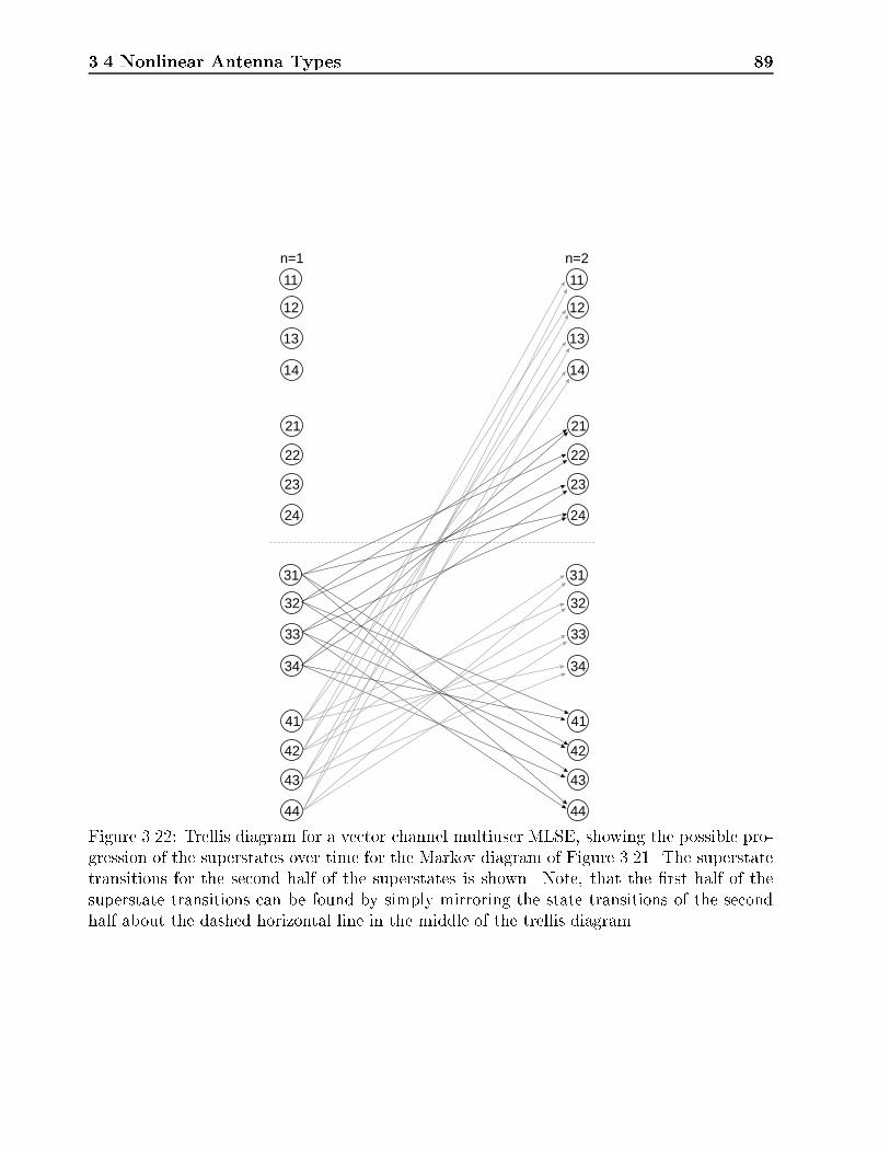
3.4 Nonlinear Antenna Types 89
11
n=1 n=2
11
21 21
31 31
41 41
12 12
22 22
32 32
42 42
13 13
23 23
33 33
43 43
14 14
24 24
34 34
44 44
Figure 3.22: Trellis diagram for a vector channel multiuser MLSE, showing the possible pro-gression of the superstates over time for the Markov diagram of Figure 3.21. The superstatetransitions for the second half of the superstates is shown. Note, that the �rst half of thesuperstate transitions can be found by simply mirroring the state transitions of the secondhalf about the dashed horizontal line in the middle of the trellis diagram.

90 Adaptation Algorithms|An Overview
vector xm;sum is given by
xm;sum = [xm(Lchannel); xm(Lchannel + 1); : : : ; xm(S)]T ; (3.156)
i.e. it is the vector of the received signals in branch m at the known positions of the trainingsequence. The ((S � Lchannel + 1)�KLchannel) block circulant matrix RTr
RTr = [RTr;1;RTr;2; : : : ;RTr;K]; (3.157)
with
RTr;k =
26664
rk(Lchannel) rk(Lchannel � 1) : : : rk(1)rk(Lchannel + 1) rk(Lchannel) : : : rk(2)
...... � � � ...
rk(S) rk(S � 1) : : : rk(S � Lchannel + 1)
37775 ;
(3.158)
contains samples of the training sequence of the k{th user intended to form the output xm;sumwith an appropriate estimate of hm.
The well know solution in a least squares sense to the problem of Equation (3.155) is thengiven by
hm = R+Trxm;sum: (3.159)
This solution is computationally rather inexpensive, since the pseudoinverse of the matrixRTr can be calculated o�{line (the training sequences are known in advance) and just needsto be stored in the receiver. Bear in mind that this is the optimum solution if and only ifthe ACF of the known signals (training sequences) is a delta function. A similar approachfor determination of the impulse responses is described in Reference [Wal95], but it utilizesa covariance approach for the determination of the impulse response of the channel.
Let the training sequence be of the form rk = [rk(S�3S1+1); rk(S�3S1+2); : : : ; rk(S�2S1); rk(1); rk(2); : : : ; rk(S � 2S1); rk(1); rk(2); : : : ; rk(S1)]
T , like the training sequences forthe GSM{system. They consist of a basic block of length S � 2S1 (=16 bits), which isselected for suitable correlation properties. The quasiperiodic continuations on each side areadded to account for the time dispersion of the channel and the time jitter of the receivedsignal burst. If the autocorrelation of the utilized training sequences is a delta pulse and thecrosscorrelation is zero (small), a rather simple approach can be utilized to determine theimpulse responses needed for MLSE detection. They are achieved simply by crosscorrelatingthe locally generated training sequence rk for the k{th user with the incoming data sequencexm;sum as
hkm;corr(n) = rk(1 : S � 2S1)Hxm;sum(n : n+ S � 2S1 � 1); n = 1; 2; : : : ; 2S1;
(3.160)
the result is the impulse response hkm;corr for transmission from the k{th user to the m{thantenna element. In practice the crosscorrelation is nonzero, i.e. the impulse responses willsu�er from some crosstalk due to the training sequences used by other co{channel users.
The advantages of using vector channel multiuser MLSE's are:

3.5 Synchronization Issues 91
� The MLSE is the optimum detector.
� It is independent of any angular separation between the users, even if the users arelocated at the same place, they can be resolved correctly by MLSE.
The disadvantages are:
� Estimation of the impulse responses su�ers from unidenti�ed co{channel interference.
� The system has to be synchronized, before MLSE processing can start.
� The computational complexity for a system serving a number of users K > 1 simulta-neously.
� It does not give DOAs, an information necessary for channel allocation and downlinkbeamforming.
3.5 Synchronization Issues
Synchronization is an important issue for any digital communications system. The di�erentalgorithmic classes require di�erent synchronization strategies:
� Linear Types:{ TR Algorithms: Synchronization has to be achieved before determination of theoptimum coe�cients (i.e. the antenna weights) in order to ensure convergence ofthe algorithm. This means that the synchronization quality directly a�ects theperformance of the whole adaptive antenna system. An optimum synchronizationstrategy for multiuser scenarios usually has a large computational complexity, as Iwill show in the following chapters. I found the adapted coe�cients and the outputSNIR of the antenna structure strongly dependent on the synchronization instant.To illustrate this statement, Figure 3.23 shows the output SNIR and the standarddeviation of the angle of the maximum of the radiation pattern versus the timingo�set of the training sequence. One signal from ' = 0� is incident at the antennaarray with M = 8 elements spaced by d=� = 0:5. The result shows that an ac-curate determination of the sampling instant for LS{based algorithms is neededespecially for phase{modulated signals ((G)MSK) in order to give high outputSNR and a small standard deviation of the estimated DOA (maximum of the ra-diation pattern). For modulation schemes like 4QAM or �=4DQPSK (Di�erentialQuadrature Phase Shift Keying), it does not matter where we sample, as long aswe are within the correct symbol. The curves for 4QAM and �=4DQPSK show astrong decrease for �o=T = 0, since this time instant marks the end of the desiredsymbol. The DOA estimates of Unitary ESPRIT, however, are independent of theactual sampling instant and the standard deviation is low.
The only exceptions to this statement is the switched beam solution and the CMA.For these algorithms synchronization can be done after beam selection (switchedbeam) or adaptation of the antenna weights (CMA).

92 Adaptation Algorithms|An Overview
−1 −0.5 0 0.5 10
5
10
15
20
25
306
Output SNIR (dB)
-Normalized timing o�set �o=T
−1 −0.5 0 0.5 110
−2
10−1
100
101
1026
�DOA (deg)
-Normalized timing o�set �o=T
(a) (b)
Figure 3.23: In uence of the synchronization on (a) the output SNIR; ���: LS adaptationfor un�ltered MSK; �:�:: LS adaptation for un�ltered 4QAM; � � �: LS adaptation forun�ltered �=4{DQPSK; |: theory; and (b) the standard deviation �DOA of the estimatedDOA; ���: LS adaptation for un�ltered MSK; �:�:: LS adaptation for un�ltered 4QAM;� � �: LS adaptation for un�ltered �=4{DQPSK; |: Unitary ESPRIT.
{ SR Algorithms: Synchronization can be done after DOA estimation and signalreconstruction, i.e. on "clean" signals | "clean", because the Signal{to{Noise{and{Interference Ratio (SNIR) of the desired signal depends on the accuracy ofthe estimated DOAs | in a relatively simple way and is therefore no criticalissue for the algorithms themselves. The antenna weights are independent of anysynchronization instant.
� Nonlinear Types: All nonlinear smart antenna types introduced in this chapter re-quire synchronization before application of the signal processing scheme, since they arebased on exploiting training sequences for the estimation of the antenna weights orchannel impulse responses. Therefore the same remarks as for TR algorithms are validfor theses schemes.
3.6 Computational Complexity
Computational complexity is an important issue for smart antenna systems. Implementedapproaches should show high{performance, be cost{e�ective and real{time solutions. Alsothey should not hinder the evolution of the systems to which they are applied.
Table 3.1 lists the computational load of the various algorithms. The graphs of the numberof complex operations (multiplications) as a function of the number of weights (number of an-tenna elementsM) are shown in Figure 3.24. A length of the training sequence L1 = L2 = 26was assumed for the graphs, so that comparison of the various approaches is possible. Thenumber of complex multiplications for calculation of the antenna weights is shown. TheCMA and the LMS algorithm are the only algorithms with a computational complexity of

3.7 Discussion 93
0 5 10 15 20 2510
2
103
104
105
1066
Complex Multiplications
-Number of antenna elements M
Figure 3.24: Number of complex multiplications as a function of the number of weights M .The length of the training sequence was set to L1 = L2 = S = 26. |: LMS, *: CMA, �:�::SQRLS, o: LS (Wiener �lter), ��: RLS, +: SR algorithms.
O(M). However, as shown, their settling time is quite large. The RLS{type algorithms havea complexity of O(M2), whereas the Wiener �lter and the LS approach have a complexity ofO(M3). This is a consequence of the matrix inversion they have to perform. Nevertheless,except for extremely largeM , the DMI solution is computationally cheaper than the conven-tional RLS algorithm. The computationally most expensive algorithms are the class of SRalgorithms, although the di�erence to DMI is modest.
3.7 Discussion
This chapter considered algorithms for the reception of multiple co{channel signals by themeans of an antenna array.
In the class of TR algorithms only the group of LS adaptation algorithms (LS, RLS, andSQRLS) and the Wiener �lter (DMI, SMI) show satisfactory performance. The convergencespeed of the class of gradient{vector estimation (like the well{known LMS) is too low forapplication to mobile radio problems.
For usual antenna dimensions in mobile communications (M � 10) the iterative algo-rithms (RLS, SQRLS, etc.) have nearly the same (or even higher) computational complexityas their direct matrix{inversion (DMI, LS) counterparts. Therefore I will concentrate on thelatter in this work, since they are not facing problems of convergence time requirements orof stability issues.
TR algorithms utilizing a training sequence need a proper synchronization before determi-nation of the antenna weights in order to provide high output SNIR. Synchronization for SR

94 Adaptation Algorithms|An Overview
MultiplicationsAlgorithm complex real
LMS 2L1M 2L1
CMA L2(2M + 1) 3L2
RLS orig. L1(4M2 + 3M) L1(2M
2 + 2M)RLS rev. L1(2M
2 + 2M) L1(2M2 + 4M)
SQRLS L1(1:5M2 + 2:5M) L1(5M � 2)
Wiener �lter, LS 13M3 + 2M2L1 � M
3-
State space 313M3 +M2(2L2 � 7)� 70
3M + 38 1
2M2 + 13
2M � 6
AdditionsAlgorithm complex real
LMS 2L1M -CMA L2(2M � 1) 2RLS orig. L1(3M
2 � 1) L1
RLS rev. L1(2M2 +M) L1
SQRLS L1(1:5M2 + 1:5M � 2) L1(2M + 3)
Wiener �lter, LS 13M3 + (2L1 � 3
2)M2 � 4
3M + 2 -
Spatial reference 113M3 +M2(2L2 � 12)� 49
3M � 5
212M2 + 3
2M � 1
DivisionsAlgorithm complex real
LMS - -CMA - -RLS orig. - 2L1
RLS rev. - L1
SQRLS - L1MWiener �lter, LS 1
2(M2 +M) -
Spatial reference M2 2M � 2
Table 3.1: Computational complexity of the various approaches. L1 denotes the length ofthe training sequence. CMA and SR algorithms do not need any training sequence, thereforethey are not limited to a speci�c length of the data vector L1. Note that L1 need not tobe equal to S, since the training sequence can be traced multiple times by the adaptationalgorithm as done for the determination of the settling times in Figure 3.6, or not all bitsof the training sequence are used for weight adaptation (e.g. for RLS). The values for theSR approach are approximate in the sense that they depend on the exact realization of theapproach and on the number of incident signals K. For the estimation of the computationalcomplexity the complex{valued fbESPRIT (forward{backward averaging ESPRIT) approachand L = M � 1 was assumed. In addition to the number of computations mentioned in thetables, fbESPRIT requires M logarithms and 4M � 4 square roots.

3.7 Discussion 95
algorithms, on the other hand, can be achieved after DOA estimation and signal separation.


Chapter 4
System Architecture | SimulationModel
In this chapter I will introduce an architecture for a BS equipped with smart antennasand derive a simulation model for a mobile communications link including a DOA{basedchannel model and smart antennas at the BS. Figure 4.1 shows the basic blocks of a BSfor an FDD system utilizing smart antennas (for up{ and downlink). I distinguish betweenthe signal processing block for the uplink and the downlink. Both blocks may work nearlyindependently, as proposed in [Far96a], or may have major parts in common. The formerapproach would give optimum performance for the link in consideration, whereas the latteris cost{e�ective. All the algorithms explained in the previous chapter can be employed atthe uplink. If linear array processing is used to recover the desired signals, the weights forthe beamformer are determined by the algorithm of choice and then they are applied to thereceived data via a highly parallel multiplier.
For the downlink, however, only linear antenna processing schemes (beamforming) canbe applied, since each mobile is intended to receive the desired signal only. I stipulate that(1) smart antennas should be introduced into existing systems without any change to theMSs, (2) no antenna array should be mounted at the mobile since it would require too muchspace, and (3) mobiles should be as cheap and lightweight as possible and should have low{power consumption, i.e. no extremely power{consuming signal processing shall be built in.Furthermore, due to security reasons, only the desired user's signal should be detected at thecorresponding MS. If an SR algorithm is applied on the uplink, its results (number of signals,DOAs, SNIRs) can readily be used for the downlink. If other approaches, like a TR or somekind of nonlinear algorithm, are used, an additional SR algorithm has to be implemented fordata extraction for the downlink. This is indicated by the dashed box in Figure 4.1.
For downlink beamforming the system needs to know the number of signals belongingto the di�erent users and the number of interferers, their DOAs, and their SNIRs. Thisinformation is also necessary for channel allocation in SDMA systems before call establishment(see also Chapter 10). Di�erent beamforming philosophies for the downlink will be examinedin Chapter 8.
My approach is to consider �rst the uplink and examine the di�erent algorithmic schemes.The most promising ones are also evaluated in terms of their downlink performance. Frommy point of view, the signal processing scheme should be as cost{e�cient as possible, sincemobile communications is a strongly market{driven business. This requires, for systems like
97

98 System Architecture | Simulation Model
Received signalx(n)
DetectionUsers’ data
dk(n)
Number ofsignals
Weights wk(n)
DOAsSNIRs
Channelallocation
Downlinkbeamforming
Data to betransmitted
dBS,k(n)
TransmittedsignalsBS(n)
Uplink
Downlink
Beamformingwk(n)
SR algorithm
MLSE
Bayesianarray
SR algorithm
TR algorithmor others
optio
nal
Figure 4.1: Architectural parts of a BS utilizing smart antennas in an FDD system.

4.1 Uplink 99
Data generator, bk(n)
Transmitter
Channel
Receiver
Comparator
Error Counter
Figure 4.2: Basic ow diagram of the simulation model for both up{ and downlink.
GSM, that as much information and algorithmic power as possible used for uplink processingshould also be utilized for the downlink. As will become clear from the next chapters, thedownlink is the bottleneck, i.e. it limits the system performance. In mobile communicationswe do not have asymmetric tra�c ow as for e.g. interactive television. Therefore it doesnot make sense to use a separate high{cost high{performance algorithm for the uplink and adi�erent approach with less performance for the downlink. Both approaches should providethe same capacity potential, a statement that points into the direction of an algorithm whoseoutput data at the uplink can be made use of for downlink beamforming.
The description of the simulation model is split into up{ and downlink. Figure 4.2 showsthe basic ow diagram that is used for both up{ and downlink.
4.1 Uplink
4.1.1 Mobile Station as a Transmitter
The transmitter generates (G)MSK{modulated signals with a TDMA protocol accordingto the GSM/DCS 1800{standard [Gsm90]. The generated signals include the data to betransmitted, the ag and tail bits, and the training sequence. The organization of the normalburst was already shown in Figure 3.1. The only distinction to an usual 2nd generation systemis that two or more mobile transmitters might be allocated at the same frequency and timeslot in the same cell. Therefore each mobile has to be assigned a unique training sequence,each of which must comply with the system speci�cations. This 26{bit midamble, originally

100 System Architecture | Simulation Model
FM-modulator
FM
Gaussian lowpassfilter
Mixer Real partextraction
Re{.}
ej(ω0τ+Φ0)
sBB(τ) sc(τ) s(τ)p(τ)
pD(τ)bn
Figure 4.3: Block diagram of the MS in transmit mode.
intended for estimation of the impulse response of the channel (equalizer training), is nowused for user identi�cation and user separation also.
Figure 4.3 shows a diagram of the simulated transmitter. The transmitted signal s(�) isgiven by
s(�) = Refsc(�)g = RefsBB(�)ej(!0�+�0)g == RefSBBej(!0�+�mod(�)+�0)g = SBB cos(!0� + �mod(�) + �0): (4.1)
In Equation (4.1) sc(�) is the complex RF signal, sBB(�) is the complex envelope, SBB isthe constant envelope of the signal, !0 is the carrier radian frequency, �0 is the initial phase(which can be assumed as zero), and �mod(�) is the excess phase de�ned by
�mod(�) = !m
�Z�1=�1
pD(�1) d�1 = !m
1Xn=�1
bn
�Z�1=�1
p(�1 � nT ) d�1; (4.2)
where the angular frequency shift !m is given by
!m =�
2T: (4.3)
pD(�) is a bipolar sequence of data pulses
pD(�) =1X
n=�1b(n)p(� � nT ); (4.4)
where b(n) is a binary, bipolar data sequence b(n) 2 [�1; 1] and p(�) is given by
p(�) =
�1 for 0 � � � T0 otherwise
(4.5)
for MSK{modulation, or [Yon88]
p(�) =1
2T
�Q
�2�pln2
BtT�� �
T
���Q
�2�pln2
BtT�1� �
T
���(4.6)
for GMSK. In Equation (4.6) Bt is the 3dB bandwidth of the GLPF (Gaussian LowPassFilter), BtT is the bandwidth{time product of the transmit GLPF, and
Q(x) =1p2�
1Zx
e�y2
2 dy =1
2
�1� erf
�xp2
��: (4.7)
I assume the mobile antenna to be an isotropic radiator that does not introduce any direc-tional pattern.

4.1 Uplink 101
e-j(ω0τ+ΦLO)
b1(n)
b2(n)
bK(n)
Dat
a U
ser 1
Dat
a U
ser 2
Dat
a U
ser K
Sig
nal p
roce
ssin
gco
nsis
ting
ofsy
nchr
oniz
atio
n;us
er s
epar
atio
nan
d de
tect
ion
orm
ultiu
ser
dete
ctio
n
1
2
3
M
sr,1(τ)
sr,2(τ)
sr,3(τ)
sr,M(τ)
Pas
sban
d fil
ter
h PB
(τ)
Bas
eban
d fil
ter
h BB
(τ)
Allp
ass
filte
r h A
P(τ
)
+
+
+
-
-
-
Ant
enna
ele
men
ts
Mix
er
Sam
pler
Sig
nal p
roce
ssin
g
Diff
eren
tial d
etec
tor
Slic
er
Tbit
Tbit
Tbit
τ= TiI
Figure 4.4: Block diagram of the BS receiver using smart antennas.
4.1.2 Channel
The channel models are taken from Chapter 2. Their speci�c characteristics are given togetherwith the simulation results.
4.1.3 Base Station as a Receiver
Assume that there are signals from K mobiles simultaneously arriving at the BS (SDMAcase). Note, this is equivalent to assuming that there are K1 < K wanted mobiles communi-cating with the BS, and K �K1 co{channel interfering signals from transmitters located inother cells arriving at the BS. As an example, for the case of SFIR, K1 = 1.
Figure 4.4 shows a block diagram of the receiver with M antenna elements. The receivedsignal, sr;m(�) at the m{th antenna element is given by
sr;m(�) = (H(m; :) � s)(t; �) + nPB(�); (4.8)
where nPB(�) is passband ST{AWGN and
(H(m; :) � s)(t; �) =KXk=1
(sk � hkm)(t; �): (4.9)
After preselection and ampli�cation | which is neglected in my simulation tool | thereceived signal is downconverted to baseband by
xBB;m(�) = sr;m(�)e�j(!0�+�LO); (4.10)

102 System Architecture | Simulation Model
where �LO is the initial phase of the local oscillator. Channel selection is performed by twoidentical lowpass �lters for the inphase (real) and quadrature (imaginary) component of thereceived signal. I use Butterworth �lter of �fth order with a 3{dB bandwidth of 1=(2T )[DAr91]. Their impulse response is denoted by hLP (�). The lowpass �lter is followed by twoidentical allpass structures with the overall impulse response hAP (�) = (hAP;1 � hAP;1)(�), forgroup delay equalization. The overall impulse response follows as
hBB(�) = (hLP � hAP )(�): (4.11)
The complex baseband signal after �ltering is therefore given by
xm(�) = (xBB;m � hBB)(�): (4.12)
The complex sampled and A/D (Analog/Digital) converted output signal xm(n) of the m{thantenna element follows as
xm(n) = xm(�)j�=nT : (4.13)
I assume that the power control tracks perfectly the large{scale fading, i.e. the signalsarriving from the di�erent users in the same tra�c channel, averaged over a certain numberof samples (i.e. di�erent propagation conditions) have the same mean power.
4.1.3.1 Signal Processing
The signal processing block contains di�erent algorithms to process the antenna output signalvector x(n). Both linear and nonlinear algorithmic approaches have been implemented andwill be compared in the subsequent chapters. Two items will be considered in the sequel: Thesynchronization procedures for di�erent algorithmic approaches and the di�erential detector.
4.1.3.1.1 Synchronization I distinguish two di�erent levels of synchronization:
� Coarse Synchronization: This is accomplished during the setup phase of a connection.Call setup is done on a channel, where only the desired mobile is present. After de-termining the mobile's power class, timing advance [Mou92], and DOAs' it is allocatedto an appropriate tra�c channel (see also Chapter 10). With the appropriate timingadvance, the mobile's transmission �ts into the burst schedule at the BS and coarsesynchronization has been achieved.
� Fine Synchronization: This is needed to determine the exact location of the receivedburst at the BS. It is done by means of the midamble of the GSM/DCS 1800 data burstto be explained below.
The key point to be stressed here is the demand di�erence between the algorithm classes:
� Algorithms utilizing a Training Sequence for Weight Adaptation: Synchronization has tobe achieved before determination of the optimum coe�cients (i.e. the antenna weights)in order to ensure convergence of the algorithm. This means that the synchronizationquality directly a�ects the performance of the whole adaptive antenna system. In thisgroup fall all TR algorithms (except CMA and switched beam) and all adaptationalgorithms for the nonlinear antenna types.

4.1 Uplink 103
� Algorithms not utilizing a Training Sequence for Weight Adaptation: Synchronizationcan be done after DOA estimation and signal reconstruction, i.e. on possibly "clean"signals ("clean", because the Signal{to{Noise{and{Interference Ratio (SNIR) dependson the accuracy of the estimated DOAs) in a relatively simple way and is therefore nocritical issue for the algorithms themselves. The antenna weights are independent ofany synchronization instant.
Three basic synchronization strategies are investigated:
(a) Joint Synchronization and Adaptation (JSA) for TR algorithms, which makes use ofthe antenna gain during synchronization.
(b) SNIR{based synchronization for SR algorithms.
(c) Correlation{based Synchronization (CS), which is suitable with both TR and SR al-gorithms.
All strategies investigated in this work are based on oversampling of the received signal. Thereceived signals are sampled with a sample rate, which is I times the bit rate. This producesI di�erent data sequences
X i = [x(i);x(i + I);x(i+ 2I); : : : ;x(i+NI)]T = [XT1&I1;i;XTr;i;XI2&T2;i]; 1 � i � I;(4.14)
where N denotes the length of the timeslot (N = 148 bits for GSM), XT1&I1 denotes thematrix containing the tail and information data of the �rst part of the burst, XTr thematrix containing the training sequence (midamble), and XI2&T2 the matrix containing theinformation and tail data of the second part of the burst (Figure 4.5).
Depending on the quality of the coarse synchronization one has to consider Nsync � Idi�erent possible "training sequences"
Mn =M(n) =XTr(n); 1 � n � Nsync; (4.15)
i.e. we search for the optimum sampling instant over several bits (we perform word andbit synchronization jointly). Note that if Nsync > I, Mn+I = [Mn;2mn;I ] is a time shiftedversion ofMn = [mn;1Mn;2], where the �rst column is omitted, the other entries are shiftedby one column and a new last entry (which is the �rst column of XI2&T2;n) is added (Figure4.5).
Now, the approaches di�er:
� JSA for TR algorithms: For each received training sequence Mn; 1 � n � Nsync
the optimum antenna weights wn for the desired user are calculated by the chosenalgorithm. Afterwards the power of the error between the known and the adaptedsequence is calculated by
"LS(n) = (r �M(n)wn)H(r �M(n) wn): (4.16)
The SNIR follows as
SNIR(n) =krk2"LS(n)
: (4.17)

104 System Architecture | Simulation Model
Data
Data DataFlagFlag
Flag FlagDataTraining
Training Sequence
26
Timeslot
T
I=4
(a)
(b)
(c)
τ
t
X(1)
M1
M2M3
X(2)
X(3)X(4)
XT1&I1 XT2&I2
XT1&I1(1)
XT1&I1(2)
XT1&I1(3)
XT1&I1(4)
XT1&I1(Nsync)
XI2&T2(1)
XI2&T2(2)
XI2&T2(3)
XI2&T2(4)
XI2&T2(Nsync)
XTr
1 FF5756 2 126
M4M5
M6
MNsync
Figure 4.5: Generation of the di�erent sequences for synchronization purposes. (a) Principleof oversampling, (b) Timeslot structure of GSM, (c) Fine structure for synchronization. I isthe oversampling factor. XT1&I1 denotes the matrix containing the tail and information dataof the �rst part of the burst, XTr the matrix containing the training sequence (midamble),and XI2&T2 the matrix containing the information and tail data of the second part of theburst. Depending on the quality of the coarse synchronization I have to consider Nsync � Idi�erent training sequences.

4.1 Uplink 105
The time instants, where local maxima of SNIR(n); 1 � n � Nsync occur
T JSA = fnj maxn=1;2;::: ;Nsync
fSNIR(n)gg; (4.18)
are the optimum sampling instants for the di�erent signals of the desired user incom-ing with di�erent delays and DOAs. Since one now knows the SNIR at the di�erentsampling instants and the delays of the associated signals, one can treat the signalsas coherent. MRC [Jak74] is therefore straightforward to implement. Assume that L1
local maxima were found by the synchronization procedure. The associated signals aredenoted by
sl1 = wTl1X l1 ; 1 � l1 � L1: (4.19)
Note that X l1 for l1 > I is given by
X l1 = [X l1�k1I(k1 + 1 : NI);x(l1 � k1I +NI + 1); : : : ;x(l1 � k1I +NI + k1)];(4.20)
where
k1 =
�l1I
�(4.21)
The signals sl1 ; 1 � l1;� L1 are now combined according to their SNIR to give the sumsignal s = [s(1); s(2); : : : ; s(n); : : : ; s(N)]T as
s(n) =L1Xl1=1
e�j(arg(p';l1 ))sl1(n)pSNIR(l1); 1 � n � N; (4.22)
which is exactly MRC as described in [Kah54]. The factor arg(p';l1) is the angle of theLeast Squares factor p';l1 between s1 and sl1 , 2 � l1 � L1, and is found as
p';l1sl1 = s1; 2 � l1 � L1: (4.23)
It is needed for combination of all signals with their proper phase.
A computational simpler approach to acquire the desired signal is to use the samplinginstant with largest SNIR only (selection diversity).
The whole procedure, however, requires a huge amount of computation. Therefore itserves in this paper as the performance bound that can be achieved by "adaptive"synchronization for TR algorithms.
� Correlation{based Synchronization for TR algorithms (CS/TR):This algorithm is basedon the midambles of the GSM normal burst. GSM speci�es eight di�erent midambles.They have been selected for an autocorrelation that is a Dirac impulse and reasonablylow cross correlation. The �rst and the last �ve bits have been added to ease channelimpulse response estimation for the equalizer. The �rst (last) �ve bits of the midambleare just repetitions of the last (�rst) �ve bits of the central 16{bit sequence. ThereforeI choose only the central 16{bit sequence v = r(6 : 21) for correlation purposes.

106 System Architecture | Simulation Model
For CS/TR the correlation vector
rCS=TR = [rCS=TR(1); rCS=TR(2); : : : ; rCS=TR(n); : : : ; rCS=TR(Nsync)]T
(4.24)
between the central training sequence, v, for the desired user and the received central16{bit midamble part in each antenna branch is calculated as
rCS=TR(n) =MXm=1
kMn(m; 6 : 21)v�k ; 1 � n � Nsync: (4.25)
The time instants, where the local maxima of this function occur, are taken as theoptimum sampling instants
T CS=TR = fnj maxn=1;2;::: ;Nsync
frCS=TR(n)gg: (4.26)
The antenna weights are therefore only calculated for those maxima, which gives atremendous saving in computational complexity.
The SNIRs for the optimum sampling instants can now be calculated according toEquations (4.16) and (4.17). MRC (Equations (4.22) { (4.23)) can therefore readily beapplied for combination of the signals. If I now assign di�erent training sequences todi�erent users in the same time/frequency channel, the sampling instants could alsobe determined if more than one user is received by the array. However, in practice theresolution capability of CS/TR is far below that of JSA. I found that usually only onemaximum exists in the correlation function, so MRC is no issue in this case.
� SNIR{based Synchronization for SR algorithms (SNIR/SR): This synchronization pro-cedure is applied after DOA estimation and signal separation has been performed.Assume that L DOAs 'l; 1 � l � L and L associated signals
sl;i = [sTl;T1&I1;i; sTl;T r;i; s
Tl;T2&I2;i]
T ; 1 � i � I (4.27)
have been determined by the SR algorithm.
Now I determine scalars p(l; n); 1 � l � L; 1 � n � Nsync, which solve the overdeter-mined set of equations
sl;T r;np(l; n) = r (4.28)
in a Least Squares{sense. Note that here I use the full{length training sequence r. TheSNIR follows therefore as
SNIR(l; n) =krk2
(r � p(l; n)sl;T r;n)H(r � p(l; n)sl;T r;n)1 � l � L; 1 � n � Nsync:
(4.29)
For n > I the training sequence of the l{th signal is
sl;T r;n = [sl;T r;n�k1I(k1 + 1 : S)T ; sl;T2&I2;n�k1I(1); : : : ; sl;T2&I2;n�k1I(k1)]T ;
(4.30)

4.1 Uplink 107
where k1 is given by Equation (4.21) and the signal for the whole timeslot follows as
sl;n = [sTl;n�k1I; sl;T2&I2;n�k1I(N + 1); : : : ; sl;T2&I2;n�k1I(N + k1)]T :
(4.31)
From this I get the matrix of SNIRs
SNIR =
26664SNIR(1; 1) SNIR(1; 2) : : : SNIR(1; Nsync)SNIR(2; 1) SNIR(2; 2) : : : SNIR(2; Nsync)
......
. . ....
SNIR(L; 1) SNIR(L; 2) : : : SNIR(L;Nsync)
37775 ;
(4.32)
where the l{th row is the SNIR versus the possible sampling instants associated withthe l{th DOA. The maxima of the SNIR of the L rows are determined and given bythe vector
snirmax =
2666664
maxn=1;2;::: ;Nsync
fSNIR(1; :)gmax
n=1;2;::: ;NsyncfSNIR(2; :)g...
maxn=1;2;::: ;Nsync
fSNIR(L; :)g
3777775 ; (4.33)
and
SNIRmax = maxl=1;2;::: ;L
fsnirmaxg (4.34)
being the absolute maximum of SNIR.
Three methods can be used for selecting the desired signals:
{ Threshold{Method: The signals belonging to rows in the SNIR{matrix having amaximum SNIR FdB below the absolute maximum SNIRmax are rejected, sincecombination of these signals does not signi�cantly improve the output SNIR.
{ Ratio of SNIRs{Method (RoS): The entries of the vector snirmax are arranged indescending order to give snirordered. Now, we determine the quantities
rsnir(l) =snirordered(l)� snirordered(l + 1)
snirordered(l + 1); 1 � l � L� 1;
(4.35)
where snirordered(l) is the l{th element of snirordered. The estimated number ofuser signals can now be found by taking the index l where the maximum of rsniroccurs,
L1RoS = maxlfrsnirg = max
lfrsnir(1); rsnir(2); : : : ; rsnir(L� 1)g:
(4.36)
{ Combination of the two methods.

108 System Architecture | Simulation Model
Assume that L1 � L rows of SNIR are left for combining, I denote this matrix bySNIR1. The positions T SNIR=SR = [TSNIR=SR(1); TSNIR=SR(2); : : : ; TSNIR=SR(L1)]
T ofthe maxima of the rows of SNIR1, which are the optimum sampling instants for thedi�erent resolved signals, are calculated as
TSNIR=SR(l1) = fnj maxn=1;2;::: ;Nsync
fSNIR1(l1)gg: (4.37)
Since the optimum sampling instants T SNIR=SR and the corresponding SNIR's areknown, again the same MRC as explained in the previous section (Equations (4.22){ (4.23)) can be utilized for combination of the signals.
� Correlation{based Synchronization for SR algorithms (CS/SR): I apply a variant ofCS also to the SR algorithms, but, as for SNIR/SR, after DOA estimation had beenperformed.
Starting with the signal vectors sl; 1 � l � L, I correlate a 16{bit part of sl;T r(i) withv as
rCS=SR(l; n) = kvHsl;T r(n : n+ 15)k; 1 � n � Nsync: (4.38)
From this I obtain the matrix of correlation values
RCS=SR =
2666666664
rTCS=SR(1)
rTCS=SR(2)...
rTCS=SR(l)...
rTCS=SR(L)
3777777775: (4.39)
The l{th row rTCS=SR(l) of RCS=SR is the correlation function associated with the l{thDOA. The maximum of RCS=SR is determined as
rCS=SR;max = maxl=1;2;::: ;L
n=1;2;::: ;Nsync
frCS=SR(l; n)g: (4.40)
I now reject all signals (i.e. rows of RCS=SR) having correlation maxima below a thresh-old value rCS=SR;th, which is a fraction Fc of the absolute maximum rCS=SR;max
rCS=SR;th =1
FcrCS=SR;max; (4.41)
since their SNIR is either too small anyway or they belong to another user. In myinvestigations I set Fc = 5. The new correlation matrix
RCS=SR;user =
2666666664
rTCS=SR;user(1)
rTCS=SR;user(2)...
rTCS=SR;user(l1)...
rTCS=SR;user(L1)
3777777775
(4.42)

4.2 Downlink 109
has only L1 rows, where L1 � L.
The positions T CS=SR = [TCS=SR(1); TCS=SR(2);: : : ; TCS=SR(L1)]T of the maxima of the
rows of RCS=SR;user, which are the optimum sampling instants for the di�erent resolvedsignals, are calculated as
TCS=SR(l1) = fnj maxn=1;2;::: ;Nsync
frCS=SR;user(l1)gg: (4.43)
Since maximum correlation does not necessarily mean maximum SNIR, the SNIR hasto be calculated to properly select the best signals. This is done within the midamble.First I determine the scalars pl1 ; 1 � l1 � L1, which solve the overdetermined equations
sl1;T r;TCS=SR(l1)pl1 = r; 1 � l1 � L1; (4.44)
in a least squares sense. The SNIR(l1) for the l1{th signal can now be determined from
SNIR(l1) =krk2
(r � pl1sl1;T r;TCS=SR(l1))H(r � pl1sl1;T r;TCS=SR(l1))
1 � l1 � L1:(4.45)
When the quantities SNIR(l1) and the positions T CS=SR are known, again the sameMRC as explained in the previous section (Equations 4.22 { 4.23) can be utilizedfor combination of the signals. In contrast to CS/TR the application of CS/SR allowsresolution of paths being only a fraction of a bit length apart, if they have been separatedby the SR algorithm, i.e. they are incident from di�erent angles.
All the steps for the corresponding synchronization procedures have to be performed for eachco{channel user independently of all other users.
4.1.3.1.2 Di�erential Detection The output signal sk(n) for the k{th user is passedto a di�erential detector. The phase angle is calculated as
�k(n) = argfsk(n)g: (4.46)
Then, the di�erence between the phase angle of the actual sampling instant n and the pre-ceding sampling instant n� 1 is calculated as
��k(n) = �k(n)� �k(n� 1) 2 [��; �): (4.47)
The estimated data bit bk(n) depends on the sign of the angle di�erence as
bk(n) = sign(��k(n)) =
�+1 for ��k(n) > 0�1 for ��k(n) � 0
: (4.48)
4.2 Downlink
4.2.1 Base Station as a Transmitter
The BS consists of a usual GMSK modulator, which generates the signals sBS;k(�) accordingto Equations (4.1) { (4.7) for the k = 1; 2; : : : ; K users to be served in the same tra�c
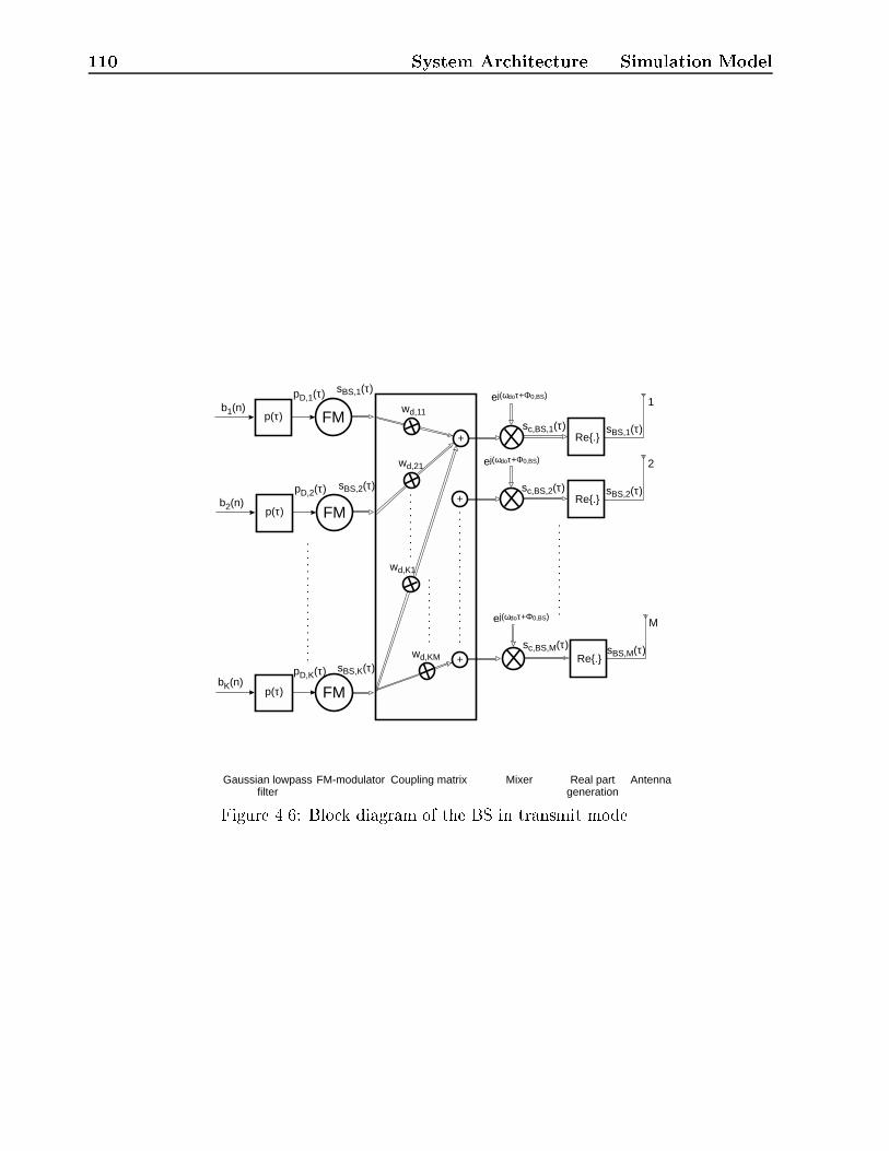
110 System Architecture | Simulation Model
pD,2(τ)
FM-modulatorGaussian lowpassfilter
Mixer Real partgeneration
FM
Re{.}
ej(ωdoτ+Φ0,BS)
sBS,K(τ)
sc,BS,M(τ)
p(τ)
pD,K(τ)
FMRe{.}
ej(ωdoτ+Φ0,BS)sBS,1(τ)
sc,BS,1(τ) sBS,1(τ)
sBS,2(τ)
sBS,M(τ)
p(τ)
pD,1(τ)b1(n)
b2(n)
bK(n)
FMRe{.}
ej(ωdoτ+Φ0,BS)
sBS,2(τ) sc,BS,2(τ)
Antenna
1
2
M
+
wd,11
wd,21
wd,K1
wd,KM
+
+
Coupling matrix
p(τ)
Figure 4.6: Block diagram of the BS in transmit mode.

4.2 Downlink 111
channel (Figure 4.6). These modulated signals are multiplied by the antenna weight vectorfor the k{th user, wd;k
sk;BS(n) = wd;ksBS;k(n); k = 1; 2; : : : ; K; (4.49)
which already has been determined by the downlink beamforming algorithm to give theuser{speci�c antenna pattern. The signal vectors for the K users are added
sBS(n) =KXk=1
sk;BS(n); (4.50)
D/A{converted and shifted to passband via
sc;BS(�) = sBS(�)ej(2�(f0+fduplex)�+�0;BS); (4.51)
where fduplex is the duplex separation between uplink and downlink, !do = 2�(f0+ fduplex) isthe downlink angular frequency, and �0;BS is the starting phase of the local oscillator in theBS.
Again, the real part sBS(�) of the analytic signal vector sc;BS(�),
sBS(�) = Refsc;BS(�)g (4.52)
is transmitted. Note, however, that in contrast to the uplink now M antennas transmit. Fora TDD (Time Division Duplex) system, these can be the same physical antenna elements asutilized for the uplink, whereas for an FDD system they may be di�erent ones (a transmitantenna mounted near the receiving one) due to today's dynamic range limitations of thereceive and transmit chains and duplexer cost.
4.2.2 Channel
The downlink channel model is the same as used for the uplink. Only the mobile has movedwithin the scatterer scenario and, in FDD systems, the carrier frequency has changed. There-fore the fading in the downlink band will be in general uncorrelated with that in the uplinkband (see Chapter 2).
4.2.3 Mobile Station as a Receiver
Since at the MS there is no smart antenna, it cannot distinguish between desired signal andinterference. In this thesis only low{rank fading channels are investigated at the downlink.Therefore I have not implemented any time{domain equalizer at the MS. The MS receiveris equivalent to one antenna branch of the BS receiver, after the A/D{converter, however,there is only one synchronization circuit, which is based on the SNIR/SR{algorithm for onereceived signal (L = 1), and a di�erential detector (Figure 4.7).

112 System Architecture | Simulation Model
e-j(ωdoτ+ΦLO)
b1(n)
Dat
a U
ser 1sr(τ)
Pas
sban
d fil
ter
h PB
(τ)
Bas
eban
d fil
ter
h BB
(τ)
Allp
ass
filte
r h A
P(τ
)
+-
Ant
enna
Mix
er
Sam
pler
Syn
chro
niza
tion
Diff
eren
tial
dete
ctor
Slic
er
Tbit
τ= TiI
Figure 4.7: Block diagram of the MS in receive mode.

Chapter 5
Basic Comparison of Algorithms forthe Uplink
The aim of this chapter is to screen the possible algorithms for uplink processing. By elaboratedetailed simulation I will justify my future selection of algorithms. Three di�erent �elds willbe covered:
� Comparison of di�erent algorithmic approaches;
� In uence of the angular separation between two users on the BER (Bit Error Rate);
� In uence of the angular spread on the BER.
The goal of this chapter is to make an initial separation of promising and less promising algo-rithms for processing of the received data in the uplink. This section gives a full comparisonof the various algorithmic approaches in terms of their raw BER, i.e. there is no interleavingand channel coding considered. The assumptions are:
� System: GSM air interface, modulation format GMSK, BtT = 0:3, K = 2 users perfrequency and time slot. Both users are assumed to have the same mean power, i.e.the CIR (Carrier{to{Interference ratio) is zero, if one user's signal is considered as thedesired one and the other user's signal as interference.
� Receive antenna: 1D{ULA with M = 10 elements having an interelement spacingof d = �=2. Figure 5.1 shows the normalized radiation pattern with equal{phaseequal{amplitude feed currents, assuming an omnidirectional radiation pattern for eachelement.
� Channel: ST{AWGN vector channel, or at Rayleigh fading vector channel, the fadingin the channels for the two users is uncorrelated. Except for Section 5.3 the angularspread is S' = 0�, i.e. there is only one discrete{valued DOA per user, the minimumangular separation between the incident signals of the two users is
'min = 2 arcsin(2
M) = 2�'max�null; (5.1)
where �'max�null is the angular distance between the maximum and the �rst null ofthe antenna pattern with equal{phase equal{amplitude feed currents. The angles of
113

114 Basic Comparison
−50 0 50−30
−25
−20
−15
−10
−5
06
Normalized antenna gain (dB)
-Azimuthal angle (deg)
Figure 5.1: Antenna pattern for an 1D{ULA with M = 10 elements and an element spacingof d=� = 0:5 with equal{phase equal{amplitude feed currents, �'max�null = 11:5�.
incidence of the two users are equally distributed between �75�, measured from arraybroadside. This value is chosen as the angular coverage region of a conventional sectorantenna (�60�) plus a margin of 15� to assist e.g. handover procedures.
� Receiver: No receiver �lter, ideal synchronization to the incoming signals. TR al-gorithms estimate the weight vector from the 26{bit GSM midamble. SR algorithmsmake use of the received data of the whole timeslot for estimation of the DOAs.
The MLSE is the optimal receiver. It serves in this chapter as the reference receiver. I willinvestigate whether
� it is practicable; and
� how the other approaches perform with respect to it.
5.1 Comparison of Di�erent Algorithms for Uplink Pro-
cessing
5.1.1 ST{AWGN Channel
Figure 5.2 shows the BERs versus the input SNR for an ST{AWGN channel. They areaveraged over both users. The theoretical BER for GMSK with MLSE{detection is given by(Appendix C)
BERth;ST�AWGN = erfc�p
SNRs;lin
�� 2
�0:5erfc
�pSNRs;lin
��2; (5.2)

5.1 Comparison of Di�erent Algorithms for Uplink Processing 115
100
10-2
10-3
10-4
10-5
10-1
-10 -5 50SNR/dB
BE
R
MLSEideal
MLSECCEN
MLSECCEI
MLSECCENI
TR Algorithm
Theory
(a)
100
10-2
10-3
10-4
10-5
10-1
-10 -5 50SNR/dB
BE
R
(b)
SR AlgorithmCS/SR
DFAideal
TR AlgorithmTheory
DFAreal
Figure 5.2: BER versus input SNR for the various algorithmic approaches in an ST{AWGNvector channel. (a) MLSE variants and TR algorithm (LS); (b) DFA variants, TR algorithm(LS), and SR algorithm (Unitary ESPRIT) with CS/SR. MLSE ideal: MLSE detector uti-lizing the ideal impulse responses; CCEN: Correlative Channel Estimation in the presenceof the desired user and Noise only; CCEI: Correlative Channel Estimation in the presenceof both users and (therefore) Interference due to the non{zero cross correlations of the train-ing sequences for the two users (no noise); CCENI: Correlative Channel Estimation in thepresence of both users with Noise and Interference due to the non{zero crosscorrelations ofthe training sequences; DFA ideal: DFA with correct symbols fed back; DFA real: DFA withdecided symbols fed back.

116 Basic Comparison
with SNRs;lin as the overall SNR on a linear scale
SNRs;lin =MSNRlin; (5.3)
where SNRlin is the input SNR at one antenna element.
The BER for the joint MLSE with ideally known impulse responses is close to theory.With correlative estimation of the impulse responses from noisy data (only the desired user'ssignal present) the performance degrades by about 2dB.
In practice, however, one has also to cope with CCI (Co{Channel Interference) due tonon{orthogonal training sequences. Appendix B introduces two optimized training sequencesfor the use within the GSM{system. These sequences were used for simulation. Despite theyare optimized in terms of minimizing CCI, there is still a certain label of CCI present. Thedegradation in BER due to non{ideal CCF's can be found in Figure 5.2 by the line labeled"MLSE CCEI". With increasing input SNR, the degradation from theory also increases.This follows since with decreasing noise contribution the constant interference contributionbecomes more and more dominant. The BER curve with the estimated impulse responsesfrom the noisy and non{ideal CCF{data (i.e. the reality) is shown by the line labeled "MLSECCENI". The values are similar to that achieved with a linear array, whose weights areadapted by a TR approach (LS), followed by a di�erential detector.
The curve for the DFA with correct symbols fed back matches closely the curve for thelinear array whose weights are adapted with a TR algorithm. If the symbols after decisionare fed back, the DFA su�ers strongly from error propagation through the feedback �lter.Under ideal conditions this should not be a problem, since the channel is ST{AWGN, i.e.there is no need for a feedback �lter (or, equivalently, the coe�cients in the feedback �ltershould be equal to zero). But due to the estimation of the coe�cients from noisy data, thecoe�cients of the feedback �lter are not equal to zero, and error propagation occurs [LeM90].
The SR algorithm (Unitary ESPRIT) with CS/SR for signal identi�cation shows lessperformance than the adaptive array.
5.1.2 Flat Rayleigh{Fading Channel
A real mobile radio channel introduces some kind of fading. Therefore my next step isto analyze the performance of the approaches in a Rayleigh{fading channel, which is themost demanding scenario. Figure 5.3 shows the BER's for this channel. Again, the sameprincipal behavior as for the ST{AWGN channel is observed. An MLSE performs well, ifthe ideal channel impulse responses are known. If they have to be estimated from noisydata, the performance is similar to a TR algorithm. If estimation is done from noisy andCCI{disturbed data, the BER does not drop under 1:5� 10�2. As a general statement, withthe used training sequences, correlation{based impulse response estimation is not applicableto this situation. If one user is in a fading dip, whereas the other is not, the impulse responseestimation for the �rst one is completely disturbed by CCI, i.e. it is wrong. This is con�rmedby the curve, which shows the BER for ideal known impulse responses, which �ts well withtheory. Appendix D gives a derivation of the number of situations, where signi�cant CCIoccurs. The result derived there �ts well with the BER level for MLSE CCEI in Figure 5.3.With improved estimation techniques ("MLSE LSCENI") for the channel impulse responses,the performance of the MLSE is near the conventional TR algorithm. Compared to theory,one loses about 3dB. The DFA su�ers from error propagation.

5.1 Comparison of Di�erent Algorithms for Uplink Processing 117
100
10-2
10-3
10-4
10-5
10-1
-10 -5 5 10 15 25 30200SNR/dB
BE
R
MLSEideal
MLSECCEN
MLSECCEI MLSE
CCENI
MLSELSCENI
TR Algorithm
Theory
100
10-2
10-3
10-4
10-5
10-1
-10 -5 5 10 15 25 30200SNR/dB
BE
R
Theory
(b)(a)
SR AlgorithmCS/SR
DFAideal
TR Algorithm
DFAreal
Figure 5.3: BER versus input SNR for the various algorithmic approaches in an Rayleigh{fading vector channel. (a) MLSE variants and TR algorithm (LS); (b) DFA variants, TRalgorithm (LS), and SR algorithm (Unitary ESPRIT) with CS/SR. MLSE ideal: MLSEdetector utilizing the ideal impulse responses; CCEN: Correlative Channel Estimation inthe presence of the desired user and Noise only; CCEI: Correlative Channel Estimationin the presence of both users and Interference due to the non{zero crosscorrelations of thetraining sequences for the two users; CCENI: CorrelativeChannel Estimation in the presenceof both users withNoise and Interference due to the non{zero crosscorrelations of the trainingsequences; LSCENI: Least Squares Channel Estimation in the presence of both users withNoise and Interference due to the non{zero cross correlations of the training sequences; DFAideal: DFA with correct symbols fed back; DFA real: DFA with decided symbols fed back.

118 Basic Comparison
5.1.3 Unidenti�ed Co{Channel Interference
I have examined an isolated system, where only two users are communicating with the BS.In reality, a BS antenna has also to cope with CCI stemming from users in neighboring cellsdue to the frequency reuse. These users are not identi�ed at the considered BS, i.e. they areco{channel interferers. Figure 5.4 shows the behavior of the di�erent algorithms versus thepower of an unidenti�ed co{channel interferer. All signals are subjected to Rayleigh{fading.The training sequence of the unidenti�ed signal was chosen randomly out of the eight trainingsequences speci�ed by the GSM standard. It was assumed that the co{channel interferingsignal arrives at the same time at the receiver as the desired signals. In a realistic scenario,there would also be a time delay between these signals, which would cause further problemsfor impulse response estimation and for model derivation for the MLSE.
The MLSE based on estimation of the channel impulse responses from the received dataremarkable loses performance with decreasing CIR (Carrier to Interference Ratio) comparedto the TR algorithm, regardless whether correlation{ or LS{based algorithms are used forimpulse response estimation. As the curves show, the performance loss is not inherent inthe MLSE{detector | the BER{curves with ideal known channel impulse responses are stillclose to theory | rather it is due to the problems with impulse response estimation. TheBER{curve for the LS{based channel impulse response estimation method (LSCENI) goes upwith decreasing CIR, for CIR=10dB it nearly reaches the BER{curve for correlative channelestimation. In contrast, the curves for TR algorithms{based array processing (linear array,DFA) show no signi�cant dependence on the CIR, since the algorithms place a null into thedirection of the interfering signal.
5.2 In uence of the Angular Separation on the BER
This section examines the in uence of the angle di�erence �', as seen from the BS, betweenthe signals of two co{channel users on the BER. Figure 5.5 shows the BERs versus the SNRfor MLSE detection of the signals for various angle di�erences �' of the incident signalsbelonging to the two users. The di�erent channel impulse response estimation strategies aretreated in the graphs. Only a slight dependence of the BER on the angular separation �' ofthe user signals exists. With decreasing separation the BER increases. This was also noticedin Ref. [Far96c]. Even for �' = 0� (i.e. the signals are incident from the same azimuthalangle) successful detection of the users' signals is possible, since the MLSE does not formbeams into the directions of desired signals and nulls out interfering ones. It just performs ajoint detection of all users.
Figure 5.6 shows the BER versus the SNR for the other adaptation strategies. These formbeams into the direction of the desired signal and put a pattern null onto the interfering one.Therefore the BER is strongly dependent on the angular separation �' of the two users.
The BER curves for TR algorithms (LS) shows a pronounced increase at the transitionfrom �' = 12:5� to �' = 7:5�. This increase can be explained by taking a look ontothe antenna pattern depicted in Figure 5.1. There it can be seen that the �rst null is at�'max�null = 11:5� away from the maximum. As long as the angular separation �' isgreater than this value, the algorithm is able to steer both a null into the direction of theinterferer and the maximum into the direction of the desired signal. If the angular separation

5.2 In uence of the Angular Separation on the BER 119
100
10-2
10-3
10-4
10-5
10-1
-10 -5 5 10 15 25 30200SNR/dB
BE
R
(b)
100
10-2
10-3
10-4
10-5
10-1
-10 -5 5 10 15 25 30200SNR/dB
BE
R
(a)
MLSEideal
MLSECCEN
MLSECCEI MLSE
CCENI
MLSELSCENI
TR Algorithm
TheoryDFAreal
SR AlgorithmCS/SR
Theory
TR AlgorithmDFAideal
100
10-2
10-3
10-4
10-5
10-1
-10 -5 5 10 15 25 30200SNR/dB
BE
R
(a)
100
10-2
10-3
10-4
10-5
10-1
-10 -5 5 10 15 25 30200SNR/dB
BE
R
(b)
MLSEideal
MLSECCEN
MLSECCEI MLSE
CCENIMLSE
LSCENI
TR Algorithm
Theory
DFAreal
SR AlgorithmCS/SR
DFAideal
TR Algorithm
Theory
100
10-2
10-3
10-4
10-5
10-1
-10 -5 5 10 15 25 30200SNR/dB
BE
R
(a)
MLSEideal
MLSECCEN
MLSECCEI
MLSECCENI
MLSELSCENI
TR Algorithm
Theory
100
10-2
10-3
10-4
10-5
10-1
-10 -5 5 10 15 25 30200SNR/dB
BE
R
(b)
TR Algorithm
TheoryDFAreal
SR AlgorithmCS/SR
DFAideal
CIR=20dB
CIR=10dB
CIR=15dB
Figure 5.4: BER versus input SNR for the various algorithmic approaches in a Rayleigh{fading vector channel with one unidenti�ed co{channel interferer. (a) MLSE variants and TRalgorithm (LS); (b) DFA variants, TR algorithm (LS), and SR algorithm (Unitary ESPRIT)with CS/SR. MLSE ideal: MLSE detector utilizing the ideal impulse responses; CCEN:Correlative Channel Estimation in the presence of the desired user and Noise only; CCEI:Correlative Channel Estimation in the presence of both users and Interference; CCENI:Correlative Channel Estimation in the presence of both users with Noise and Interference;LSCENI: Least Squares Channel Estimation in the presence of both users with Noise andInterference; DFA ideal: DFA with correct symbols fed back; DFA real: DFA with decidedsymbols fed back.
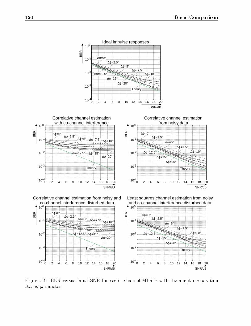
120 Basic Comparison
10-2
10-2
10-2
10-2
10-2
10-3
10-3
10-3
10-3
10-3
10-4
10-4
10-4
10-4
10-4
100
100
100
100
100
10-1
10-1
10-1
10-1
10-1
0
0
0
0
0
SNR/dB
SNR/dB
SNR/dB
SNR/dB
SNR/dB
BE
R
BE
RB
ER
BE
RB
ER
Theory
Theory
Theory
Theory
Theory
2
2
2
2
2
4
4
4
4
4
6
6
6
6
6
8
8
8
8
8
10
10
10
10
10
12
12
12
12
12
14
14
14
14
14
16
16
16
16
16
18
18
18
18
18
20
20
20
20
20
∆ϕ=20°
∆ϕ=20°
∆ϕ=20°
∆ϕ=20°
∆ϕ=20°
∆ϕ=15°
∆ϕ=15°
∆ϕ=15°
∆ϕ=15°
∆ϕ=15°
∆ϕ=10°
∆ϕ=10°
∆ϕ=10°
∆ϕ=10°
∆ϕ=10°
∆ϕ=12.5°
∆ϕ=12.5°
∆ϕ=12.5°
∆ϕ=12.5°
∆ϕ=12.5°
∆ϕ=7.5°
∆ϕ=7.5°
∆ϕ=7.5°
∆ϕ=7.5°
∆ϕ=7.5°
∆ϕ=2.5°
∆ϕ=2.5°
∆ϕ=2.5°
∆ϕ=2.5°
∆ϕ=2.5°
∆ϕ=5°
∆ϕ=5°
∆ϕ=5°
∆ϕ=5°
∆ϕ=5°
∆ϕ=0°
∆ϕ=0°
∆ϕ=0°
∆ϕ=0°
∆ϕ=0°
Ideal impulse responses
Correlative channel estimationfrom noisy data
Correlative channel estimationwith co-channel interference
Correlative channel estimation from noisy andco-channel interference disturbed data
Least squares channel estimation from noisyand co-channel interference disturbed data
Figure 5.5: BER versus input SNR for vector channel MLSEs with the angular separation�' as parameter.

5.2 In uence of the Angular Separation on the BER 121
10-2
10-2 10-2
10-210-2
10-2
10-3
10-3 10-3
10-310-3
10-3
10-4
10-4 10-4
10-410-4
10-4
100
100 100
100100
100
10-1
10-1 10-1
10-110-1
10-1
0
0 0
00
0
SNR/dB
SNR/dB SNR/dB
SNR/dBSNR/dB
SNR/dB
BE
RB
ER
BE
RB
ER
BE
R
BE
R
Theory
Theory Theory
TheoryTheory
Theory
2
2 2
22
24
4 4
44
46
6 6
66
68
8 8
88
810
10 10
1010
1012
12 12
1212
1214
14 14
1414
1416
16 16
1616
1618
18 18
1818
1820
20 20
2020
20
∆ϕ=20°
∆ϕ=20° ∆ϕ=20°
∆ϕ=20°
∆ϕ=20°
∆ϕ=20°∆ϕ=15°
∆ϕ=15° ∆ϕ=15°
∆ϕ=15°
∆ϕ=15°
∆ϕ=15°
∆ϕ=10°
∆ϕ=10° ∆ϕ=10°
∆ϕ=10°
∆ϕ=10°
∆ϕ=10°
∆ϕ=12.5°
∆ϕ=12.5° ∆ϕ=12.5°
∆ϕ=12.5°
∆ϕ=12.5°
∆ϕ=12.5°
∆ϕ=7.5°
∆ϕ=7.5° ∆ϕ=7.5°
∆ϕ=7.5°
∆ϕ=7.5°
∆ϕ=7.5°∆ϕ=2.5°
∆ϕ=2.5° ∆ϕ=2.5°
∆ϕ=2.5°∆ϕ=2.5°
∆ϕ=2.5°
∆ϕ=5°
∆ϕ=5° ∆ϕ=5°
∆ϕ=5°∆ϕ=5°
∆ϕ=5°
∆ϕ=0°
∆ϕ=0° ∆ϕ=0°
∆ϕ=0°∆ϕ=0°
∆ϕ=0°
TR algorithm with LS weight adaptation
DFA with LS weight adaptationand ideal symbols feed back
DFA with LS weight adaptationand decided symbols feed back
SR algorithm (Unitary ESPRIT) with CS/SRMDL criterion
SR algorithm (Unitary ESPRIT) with CS/SRRoE criterion
SR algorithm (Unitary ESPRIT) with CS/SRnumber of incident signals known
Figure 5.6: BER versus input SNR for TR and SR algorithms and the DFA with the angularseparation �' as parameter.

122 Basic Comparison
�' is smaller than 11:5�, the algorithm loses gain into the direction of the desired signalby steering a null into the direction of the interfering signal. For �' = 0� no successfulcommunication between the two users and the BS is possible.
The BER curves for SR algorithms are strongly dependent on the quality of the estima-tion of the number L of incident signals and on the signal identi�cation strategy. For theconsidered case, the MDL criterion with CS/TR does not give as good results as the RoEcriterion with CS/SR or the (of course, unrealistic) assumption that the number of signalsis known. For comparison with the curves for the TR algorithms I will take the two latterresults. The pronounced increase in BER for SR algorithms is at the same point as for TRalgorithms, which also con�rms that this is an e�ect related to the used antenna (antennapattern) and not of the applied algorithm. For �' < 10� TR algorithms outperform SRalgorithms, whereas for �' > 10� just the opposite e�ect occurs. This can be explained asfollows: The beamforming algorithm for SR algorithms (incorporated for reconstruction ofthe signals) places unity gain (which is not necessarily the maximum!) into the directionof the desired signals and nulls onto the interferers. This may result in an antenna patternhaving its maximum into a direction, where no signal is coming from, especially if the angularseparation is small. For small angular separations, however, it might be more appropriatein terms of output SNIR not to put a full null into the direction of the interference, sincedue to the non{zero width of the antenna pattern the desired signal also is attenuated. TRalgorithms implicitly make a compromise between these two e�ects, since they minimize somekind of error, i.e. they maximize the SNIR, at the array output. This makes them performingbetter as than SR algorithms for small angular separations. For large angular separations thestrategy of the beamformer for SR algorithms is quite successful and outperforms TR algo-rithms. TR algorithms estimate the antenna weights from a �nite{length training sequence.Therefore their performance is suboptimum for the whole GSM timeslot. SR algorithms, onthe other hand use the data of the whole timeslot for determination of the DOAs. This makesthem more robust concerning to noise contributions.In noiseless environments, an in�nite deep null onto the interfering signal would allow toreconstruct the wanted signal with maximum SNIR. But, since the SNR is �nite, in�niteattenuation of the interfering signal means also attenuation of the wanted signal near to (oreven below) the noise oor, therefore also the SNIR is decreased. Consecutively, it does notmake sense to place a null, which is much deeper than the noise oor, onto an interferingsignal.
DFAs with correct symbols fed back show the same basic behavior as TR algorithms,i.e. they are also not able to separate signals incident from the same direction. DFAs withdecided symbols fed back su�er strongly from error propagation in this application.
5.3 In uence of the Angular Spread S' on the BER
TR algorithms combine the output signals of the antenna elements to minimize a predeter-mined performance measure. SR algorithms assume that the angular spread of the incidentwaves is S' = 0�. To investigate the in uence of a non{zero angular spread S', I have as-sumed a uniform PDF of the incoming wave with p('�'0) = 1=(2�) for �� � '�'0 < �,around the nominal DOA '0.
Figure 5.7 shows the BERs versus the angular width of the incident signals. In general,

5.3 In uence of the Angular Spread S' on the BER 123
TR algorithm with LS weight adaptationSR algorithm (Unitary ESPRIT) with CS/SR
MDL criterion
SR algorithm (Unitary ESPRIT) with CS/SRRoE criterion
SR algorithm (Unitary ESPRIT) with CS/SRnumber of incident signals known
10-2 10-2
10-210-2
10-3 10-3
10-310-3
10-4 10-4
10-410-4
10-5 10-5
10-510-5
100 100
100100
10-1 10-1
10-110-1
0 0
00
SNR/dB SNR/dB
SNR/dBSNR/dB
BE
R
BE
RB
ER
BE
R
Theory Theory
TheoryTheory
5 5
55
10 10
1010
15 15
1515
25 25
2525
30 30
3030
20 20
2020
∆=0°∆=0°
∆=0° ∆=0°
∆=1°∆=1°
∆=1° ∆=1°
∆=2°∆=2°
∆=2° ∆=2°
∆=0.5°∆=0.5°
∆=0.5° ∆=0.5°
∆=3°∆=3°
∆=3°
∆=3°
∆=4°∆=4°
∆=4°∆=4°
∆=5°∆=5°
∆=5°∆=5°
∆=6°∆=6°
∆=6°∆=6°
∆=7°∆=7°
∆=7° ∆=7°
Figure 5.7: BER versus input SNR for TR and SR algorithms with the angular width � ofthe incident signals as parameter.

124 Basic Comparison
7 5 3 1 0
0
10
20
30
0
1
2
3
4
5
6
Nu
mb
er o
f es
tim
ated
si
gn
als,
MD
L c
rite
rio
n
Angular width (deg)
SNR (dB)
Figure 5.8: Number of incident signals determined by the MDL criterion with the angularwidth � and the input SNR as parameter.
algorithm performance decreases with increasing angular spread. For TR algorithms theincrease is about a factor of 3, if the angular spread increases from S' = 0� (� = 0�) toS' = 4� (� = 7�).
The situation is much more dramatic for SR algorithms. Using the MDL criterion forestimation of the number of incident signals L, the increase in BER is about a factor 25(for SNR=30dB). The situation becomes even more dramatic, if the RoE criterion is used.Here, the increase in BER is nearly a factor 100(!) for SNR=30dB. The largest increase inBER show the curves for assuming the number of incident signals, L, as known. The curvesrun against a threshold dependent on the angular spread S'. This shows that assuming thenumber of incident signals as known is an extremely sensitive assumption, especially if theangular extension of the incident signals is non{zero.
The mean value for the number of estimated signals L with the MDL criterion is shownin Figure 5.8. For small angular spreads the number is L = 2, the exact number of incidentsignals. With increasing angular spread S' and increasing input SNR the number of estimatedsignals increases also, although there are only two signals, associated with a (large) angularspread, present. This is the reason for the better performance of SR algorithms utilizingMDL instead of RoE or assuming the number of signals as �xed.
5.3.1 Accuracy of the estimated DOAs for TR and SR Algorithms
Another key parameter that has to be watched, is the accuracy of the estimated DOAs. Un-fortunately, TR algorithms do not give a DOA of the signal directly. Therefore I determinedthe angular location of the maximum of the antenna pattern calculated from the weights,which were determined by the TR algorithm. Figure 5.9 shows the standard deviation of thedi�erence between the angle of the maximum of the antenna pattern and the ideal DOA. Thestandard deviations are rather high, even for � = 0�, so I have to take a closer look on thate�ect. Figure 5.10 shows a set of histograms for the di�erence between the ideal and the es-timated DOA for � = 0� for various SNRs. Figure 5.10a shows the histograms for this angledi�erence for estimation of the antenna weights from the noisy GSM training sequence. ForFigure 5.10b the length of the training sequence was doubled to determine whether the length

5.3 In uence of the Angular Spread S' on the BER 125
7 5 3 1 0
0
10
2030
0
5
10
15
20
25
Sta
nd
ard
dev
iati
on
o
f th
e es
tim
ated
D
OA
s (d
eg)
Angular width (deg)
SNR (dB)
Figure 5.9: Standard deviation of the maximum of the antenna pattern determined by TRalgorithms with the angular width � and the input SNR as parameter.
itself a�ects the estimation quality. 2000 simulation runs have been performed to computethe results. Figure 5.11 shows the standard deviations for the angle di�erence between theideal and the estimated DOA for � = 0� for various SNRs. All curves show that the maximaof the radiation pattern determined by the LS{approach does not necessarily point into thedirection of the desired signal, although it is within a window of about 10� around the idealDOA. A minimum of the standard deviation can be observed around SNR=30dB. Here thenoise contribution is small enough to force a pattern maxima into the direction of the desiredsignal, but large enough not to cause signi�cant in uence on the estimation quality. Withincreasing SNR the standard deviation increases again. This is caused by the reason thatthe goal of LS (or, equivalently the Wiener Filter) is to minimize the contribution of theinterference and not to steer a maximum into the direction of the desired signal [N�r96].
A more mathematical justi�cation is as follows: TR algorithms determine the weightsfrom a system of equations. The system consists at least ofM equations forM unknowns. If| as in my case | the number of incident signals, L, is below M and there is no noise, thecoe�cient matrix is rank de�cient. This means that only L of the M rows (or columns) arelinearly independent. In consequence, only L weights can be meaningfully determined, theothers can be set to arbitrary values. If the noise increases, the rank of the coe�cient matrixincreases also. Therefore the weights approach the optimum solution with increasing noisecontributions up to the level, where the noise is too large not to in uence the determinationprocess (which is about SNR=20{30dB in my simulations). Figure 5.12 shows the standarddeviation of the di�erence between the estimated and the real DOAs for utilizing a SRalgorithm and the MDL criterion. For � < 2� and SNR�10dB the performance is excellent.The values can be used directly for downlink beamforming and channel allocation. However,with increasing angular width � the performance also decreases, leaving the estimated DOAsnot always applicable for downlink beamforming.
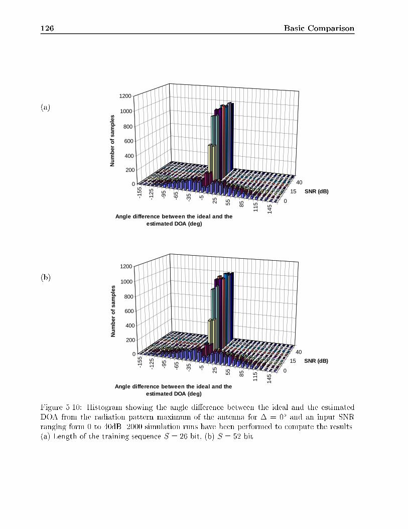
126 Basic Comparison
-155
-125
-95
-65
-35
-5
25 55 85
115
145
0
15
400
200
400
600
800
1000
1200
Nu
mb
er o
f sa
mp
les
Angle difference between the ideal and the estimated DOA (deg)
SNR (dB)
(a)
-155
-125
-95
-65
-35
-5 25 55 85
115
145
0
15
400
200
400
600
800
1000
1200
Nu
mb
er o
f sa
mp
les
Angle difference between the ideal and the estimated DOA (deg)
SNR (dB)
(b)
Figure 5.10: Histogram showing the angle di�erence between the ideal and the estimatedDOA from the radiation pattern maximum of the antenna for � = 0� and an input SNRranging form 0 to 40dB. 2000 simulation runs have been performed to compute the results.(a) Length of the training sequence S = 26 bit, (b) S = 52 bit.

5.3 In uence of the Angular Spread S' on the BER 127
0 10 20 30 40 50 6010
0
101
102
6Standard deviation (deg)
-Input SNR (dB)
���S = 52 bit
���S = 26 bit
Figure 5.11: Standard deviation for the angle di�erence between the ideal and the estimatedDOA for � = 0� for various SNRs for a TR algorithm. Two lengths S of the training sequenceare investigated.
7 5 3 1 0
0
10
2030
02468
1012141618
Sta
nd
ard
dev
iati
on
o
f th
e es
tim
ated
D
OA
s (d
eg)
Angular width (deg)
SNR (dB)
Figure 5.12: Standard deviation of the estimated DOAs for an SR algorithm (MDL criterion)with the angular width � and the input SNR as parameter.

128 Basic Comparison
5.4 Conclusions
The simulation results in this chapter show that not all structures for smart antenna signalprocessing are promising for mobile communications.
All nonlinear antenna types fail in the investigated simple scenario:
� The DFA su�ers strongly from error propagation. The only situation, where a DFAwould be helpful, is a situation where signi�cant signals are incident from nearly thesame direction (�' < 6� for an 1D{ULA with d=� = 0:5 and M = 8, see Chapter 3).But, as stated in [Kle96a], in mobile communications usually di�erent delay times �are related to di�erent DOAs '. Therefore there is no cogent reason to use DFAs.
� The Bayesian arrays are ruled out by the results of Ref. [Upc94], therefore I have nottaken a look on them in this work.
� MLSE's perform excellent, if the exact impulse responses for the di�erent channels areknown. If they have to be estimated from the received data, which is the case for a real{world mobile communications system, an MLSE does not perform signi�cantly betterthan a linear array utilizing a TR algorithm, if used within the current GSM standard.The correlation properties of the modulated training sequences are too bad to enablereliable determination of the impulse responses. Furthermore, MLSEs su�er from theproblem of unidenti�ed co{ or adjacent{channel interferers. Their presence degradesthe estimation of the impulse response considerably, which leads to high BERs. Sincea certain amount of such interference will be present especially in small reuse factorsystems, where smart antennas are designed for, multiuser MLSEs are not the way togo for in the current GSM standard.
What remains are linear processing schemes. These schemes show promising performance.SR algorithms with correlation{based signal identi�cation do not give promising results inRayleigh{fading channels, therefore I will concentrate in the sequel on SR algorithmswith signal identi�cation based on SNIR{criteria. The performance of SR algorithmsis strongly dependent on the angular spread S', with increasing angular spread S' theirperformance degrades signi�cantly. Therefore they are only applicable to situations, whereonly limited angular spreads exist, i.e. in macrocells.
TR algorithms perform well nearly independent of the actual angular spread. They areapplicable to any scenario independent whether DOAs exist or not.
The DOAs derived from SR algorithms are much more precise for small angular spreadsthan the ones deduced from the maximum of the antenna pattern derived by the applicationof TR algorithms. This is an important fact for the downlink to be addressed in Chapter8. Furthermore, the quality of the DOA estimates by TR algorithms depends on the inputSNR. Above a certain threshold (around 30dB), with increasing input SNR the quality of theestimates degrades. This follows, since TR algorithms minimize some kind of error, i.e. theyput nulls onto the interfering signals, however, they steer a maximum towards the wantedsignal only if the input SNR is low.
5.4 Conclusions 129
While the BER obtained with TR algorithms at high input SNRs is excellent, the maximumof the antenna pattern does not always point into the direction of the desired signal. So forTR algorithms the BER{behavior and the quality of the determined "DOAs" (since theyare derived from the location of the maximum of the antenna pattern) has to be clearlydistinguished. While the former is excellent the latter has to be handled with care.
For angular spreads S' > 2� the standard deviation of the estimated DOAs is ratherhigh. What remains for downlink beamforming for small{output SNIR cases, is to utilizee.g. an antenna with �xed beams, where the one which received the most useful power inthe uplink is also used for the downlink. Another alternative is to apply more sophisticateddetection schemes at the MS (antenna diversity, MRC with two or maybe three antennas, orinterference cancellation).


Chapter 6
Comparison of Linear AdaptationSchemes
This chapter examines the remaining linear algorithmic approaches in terms of the more real-istic channel models introduced in Chapter 2. Additionally, in the second part of this chapter,the ideal synchronization assumption is relaxed and the in uence of di�erent synchronizationschemes on the BER is determined.
In the �rst part I will examine the performance of the di�erent linear schemes for a systemusing MSK modulation and ideal synchronization. I will analyze (1) the minimum angularseparation of two users necessary to give reasonable good BERs, (2) the in uence of di�erentsignal detection schemes on the performance of Unitary ESPRIT, and (3) the in uence ofmutual coupling on the performance of the algorithms.
In the second part of this chapter I will analyze a full GSM system utilizing GMSK withBtT = 0:3 with oversampling at the receiver and adaptive synchronization.
6.1 Performance of Linear Adaptation Schemes for a
Channel Model including DOAs and an Angular
Spread
In this section I will investigate the performance of Switched Beam, a TR algorithm (LS{approach), and an SR algorithm (Unitary ESPRIT). The algorithms have already been ex-plained in Chapter 3. Here, I will focus on some details concerning detection for SR algorithmsonly. I investigate three detection schemes:
1. The conventional SNIR{based synchronization scheme introduced in Chapter 4. Sincethe signals are incident from a nominal DOA associated with an angular spread, ratherthan from one discrete direction, two or more estimated DOAs may be close{by. Thisgives considerable problems for beamforming. The beamforming algorithm incorpo-rated for reconstruction of the signals places unity gain (which is not necessarily themaximum!) into the direction of the desired signals and nulls onto the interferers. Thismay result in an antenna pattern pointing into a direction where no signal is comingfrom. In the derivation of the model{order determination criteria MDL and AIC it isassumed that the signals only come from the determined discrete directions and have
131
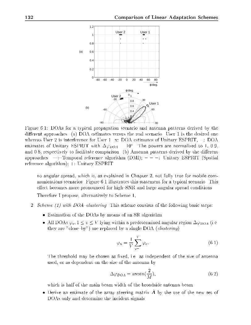
132 Comparison of Linear Adaptation Schemes
0.2
0.4
0.6
0.8
1
30-30
60-60
90-90
0
0
0.2
0.4
0.6
0.8
1
1.2
-80 -60 -40 -20 0 20 40 60 80
ϕ/deg.
ϕ/deg.
(a)
(b)
User 1
User 1
User 2
User 2
Figure 6.1: DOAs for a typical propagation scenario and antenna patterns derived by thedi�erent approaches. (a) DOA estimates versus the real scenario. User 1 is the desired onewhereas User 2 is interference for User 1. x: DOA estimates of Unitary ESPRIT, +: DOAestimates of Unitary ESPRIT with �'DOA = 10�. The powers are normalized to 1, 0.9,and 0.8, respectively to facilitate comparison. (b) Antenna patterns derived by the di�erentapproaches. |: Temporal reference algorithm (DMI); � � �: Unitary ESPRIT (Spatialreference algorithm); +: Unitary ESPRIT
no angular spread, which is, as explained in Chapter 2, not fully true for mobile com-munications scenarios. Figure 6.1 illustrates this statement for a typical scenario. Thise�ect becomes more pronounced for high{SNR and large angular spread conditions.
Therefore I propose, alternatively to Scheme 1,
2. Scheme (1) with DOA{clustering. This scheme consists of the following basic steps:
� Estimation of the DOAs by means of an SR algorithm.
� All DOAs 'v; 1 � v � V lying within a predetermined angular region �'DOA (i.e.they are "close{by") are replaced by a single DOA (clustering)
'n =1
V
VXv=1
'v: (6.1)
The threshold may be chosen as �xed, i.e. as independent of the size of antennaused, or as dependent on the size of the antenna by
�'DOA = arcsin(2
M); (6.2)
which is half of the main beam width of the broadside antenna beam.
� Derive an estimate of the array steering matrix A by the use of the new set ofDOAs only and determine the incident signals.
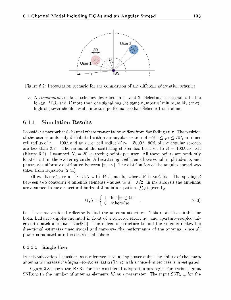
6.1 Channel Model including DOAs and an Angular Spread 133
User 1
BS
User 2
r1
r2
2R
Figure 6.2: Propagation scenario for the comparison of the di�erent adaptation schemes.
3. A combination of both schemes described in 1. and 2. Selecting the signal with thelowest BER, and, if more than one signal has the same number of minimum bit errors,highest power should result in better performance than Scheme 1 or 2 alone.
6.1.1 Simulation Results
I consider a narrowband channel where transmission su�ers from at fading only. The positionof the user is uniformly distributed within an angular section of �70� � 'k � 70�, an innercell radius of r1 = 100� and an outer cell radius of r2 = 5000�. 90% of the angular spreadsare less than 2:2�. The radius of the scattering cluster has been set to R = 100� as well(Figure 6.2). I assumed Ns = 20 scattering points per user. All these points are randomlylocated within the scattering circle. All scattering coe�cients have equal amplitudes al, andphases �l uniformly distributed between [�;��[. The distribution of the angular spread wastaken from Equation (2.41).
All results refer to a 1D{ULA with M elements, where M is variable. The spacing dbetween two consecutive antenna elements was set to d = �=2. In my analysis the antennasare assumed to have a sectoral horizontal radiation pattern f(') given by
f(') =
�1 for j'j � 90�
0 otherwise; (6.3)
i.e. I assume an ideal re ector behind the antenna structure. This model is suitable forboth, halfwave dipoles mounted in front of a re ector structure, and aperture{coupled mi-crostrip patch antennas [Kuc96a]. The re ection structure behind the antenna makes thedirectional estimates unequivocal and improves the performance of the antenna, since allpower is radiated into the desired halfsphere.
6.1.1.1 Single User
In this subsection I consider, as a reference case, a single user only. The ability of the smartantenna to increase the Signal{to{Noise Ratio (SNR) in this noise{limited case is investigated.
Figure 6.3 shows the BERs for the considered adaptation strategies for various inputSNRs with the number of antenna elements M as a parameter. The input SNRk;in for the

134 Comparison of Linear Adaptation Schemes
100
10-2
10-3
10-4
10-1
0 2 4 6 8 10 12 14 16 18 20
SNR/dB
BE
R
M=1
M=1, Theory
M=8
M=8
M=5
M=5M=2M=2
BER criterion SB
SB
SB
SB
TR
TR
TR
SR
SR
SR
Figure 6.3: BER versus SNR for a single user. TR: Temporal reference algorithm (DMI),o: LS, (SQ)RLS; SB: Switched beam (BER and power criterion); SR: Spatial referenceAlgorithm. M denotes the number of antenna elements.
k{th user is de�ned as
SNRk;in =Pk2�2
; (6.4)
where �2 is the noise power and Pk is the power of the k{th user incident at the referenceelement (usually element #1) given by
Pk = Et"E(
NsXns=1
Pns
)#; (6.5)
where Ef:g stands for averaging over the small{scale fading and Etf:g for averaging over theabsolute time t.
The BERs are averaged over arbitrary user positions within the annular coverage regionand the small{scale fading. This includes an averaging over the possible angular spreads also.
The theoretical achievable BERth for the considered modulation scheme in a at fadingchannel follows as (see Appendix C)
BERth =1
2
"1�
rSNR
SNR + 2
#; (6.6)
where SNR is the signal{to{noise ratio on a linear scale given by
SNR =MSNRin: (6.7)
The curve forM = 1 agrees well with this theory (6.6). The curves forM = 5 andM = 8 how-ever di�er appreciable from the theoretical at fading model (Figure 6.3). This is explainedas follows: The signal fading at the antenna elements is correlated, where the correlationdecreases with increasing distance of two considered antenna elements, with decreasing angleof incidence (measured from array broadside) of the signals, and with increasing angular
6.1 Channel Model including DOAs and an Angular Spread 135
spread (Chapter 2). This means that with increasing antenna dimensions the fading at thereference element and the last element of the array becomes more and more uncorrelated.The adaptation algorithms can make use of this fact to improve link performance. For TRalgorithms operating in low{SNR environments (SNR < 10dB) errors in the determination ofthe optimum weight vector from the noisy data mask the positive e�ect of correlation withinthe fading.
The performance di�erence between the three algorithms is small: at SNR = 16dB andM = 5 (M = 8), the BER di�ers by a factor of 1.2 (1.5) at most. Switched beam with acombination of power and BER criteria and the SR algorithm perform slightly better thanthe TR algorithm. This may be attributed to the fact that the TR algorithm estimates theweight vector from the 26{bit midamble. As we move toward the ends of the timeslot in thenon{stationary channel the received midamble becomes less and less representative for thechannel. Channel tracking | which is necessary for systems like D{AMPS (DigitalAdvancedMobile Phone System) [Win96] | can improve the performance of TR algorithms.
The nominal DOA of the incident signals is the only quantity being stationary. This givesadvantages for DOA{based approaches for this speci�c scenario. Unitary ESPRIT performsbetter than the Switched beam approach, since it can place a beam at every desired angularlocation, whereas the other can only steer a beam in a limited number of angular directions.
Switched beam with only a BER criterion performs markedly worse. The reason is thatthere are several beam positions where the BER becomes minimum. The algorithm simplyselects the �rst of them as the desired position, which might be suboptimum.
For the single user scenario (without interference) the power criterion alone works equallywell as the combined BER/power criterion.
TR structures based on either DMI, the deterministic Least Squares (LS) approach, onthe RLS, and on the SQRLS are equivalent. The BER curves coincide.
The results show that the performance of SR structures is not impaired by the propagationmechanisms of the mobile radio channel, particularly not by the spread{out DOAs.
6.1.2 Two Users
The simplest SDMA scenario involves two users in the same tra�c channel. With a con-ventional detector the BER for one user would be 0.25, even for in�nite SNR (see AppendixE).
If two users are too close in angle (note that this does not necessarily mean too closein space!), they cannot be separated by linear antenna processing | such a scenario iscalled poorly separable [Far96b]. A mathematical de�nition for spatial separability is givenin Appendix F. So, if the angular separation of the two users reaches a given lower angularthreshold 'th, a handover of one user to a di�erent tra�c channel has to be performed. Thisthreshold, of course, in uences the capacity: the higher the threshold, the lower the capacity.
Figure 6.4 shows the BER experienced by one of the two users, in the same tra�c channel,as a function of the
� adaptation scheme;
� number of antenna elements, M ; and
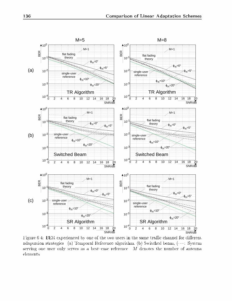
136 Comparison of Linear Adaptation Schemes
100 100
100
100100
100
10-2 10-2
10-2
10-210-2
10-2
10-3 10-3
10-3
10-310-3
10-3
10-4 10-4
10-4
10-410-4
10-4
10-1 10-1
10-1
10-110-1
10-1
0 0
0
00
0
2 2
2
22
2
4 4
4
44
4
6 6
6
66
6
8 8
8
88
8
10 10
10
1010
10
12 12
12
1212
12
14 14
14
1414
14
16 16
16
1616
16
18 18
18
1818
18
20 20
20
2020
20
SNR/dB SNR/dB
SNR/dB
SNR/dBSNR/dB
SNR/dB
BE
R
BE
RB
ER
BE
R
BE
RB
ER
M=5
TR Algorithm TR Algorithm
Switched BeamSwitched Beam
SR Algorithm SR Algorithm
M=8
M=1 M=1
M=1M=1
M=1 M=1
ϕth=5°ϕth=5°
ϕth=5°ϕth=5°
ϕth=5°ϕth=5°
ϕth=20° ϕth=20°
ϕth=20°ϕth=20°
ϕth=20°ϕth=20°
ϕth=10° ϕth=10°
ϕth=10°ϕth=10°
ϕth=10°ϕth=10°
ϕth=0°ϕth=0°
ϕth=0°ϕth=0°
ϕth=0°ϕth=0°
single-userreference
flat fadingtheory
flat fadingtheory
flat fadingtheory
flat fadingtheory
flat fadingtheory
flat fadingtheory
single-userreference
single-userreference
single-userreference
single-userreference single-user
reference
(a)
(b)
(c)
Figure 6.4: BER experienced by one of the two users in the same tra�c channel for di�erentadaptation strategies. (a) Temporal Reference algorithm, (b) Switched beam, (� � � : Systemserving one user only serves as a best{case reference. M denotes the number of antennaelements.

6.1 Channel Model including DOAs and an Angular Spread 137
� angular threshold value, 'th.
The performance of the TR approach is excellent: For an angular threshold as low as 10�,an array with M = 8 elements is su�cient to obtain nearly the same performance as in thesingle{user case. With M = 5 antenna elements this best{case reference can be approachedto within a factor of 1.6 in BER. WithM = 8 elements the adaptive array is able to separatetwo co{channel users that are as close as 5� in angle.
The �gure also demonstrates that Switched beam and SR structures perform worse thanthe TR structure. Switched beam uses a given set of beams and selects the best of them inaccordance to some criterion. Since this approach cannot place the maximum in the "best",i.e. desired, direction and a concomitant zero in the unwanted angular section, interferenceis always higher than for the adaptive array approach. This leads to the observed increasein BER, especially for high{SNR conditions where the curves saturate.
For the SR structure the number of DOAs (incoming signals) detected by the MDL{ andthe AIC{criterion is always greater than or equal to the number of users (in our case two),i.e. the DOAs are necessarily not discrete.
Both criteria perform equally well in terms of BER; therefore the curves labeled with"Unitary ESPRIT" apply to both the AIC or the MDL criterion.
Figure 6.5a shows the BERs with �'DOA = 10�, where I applied Scheme 2 to detect theuser's signal. For angular separations of the two users of less than 10� this approach performsworse since the two DOAs cannot be resolved correctly.
At �rst glance, no signi�cant improvement of introducing �'DOA can be observed. How-ever, the situations where the two schemes in Figure 6.4c and 6.5a give errors, are distinct.Consequently, I apply Scheme 3, which I refer to as "BER{driven selection" (Figure 6.5b). Itperforms best of all algorithms and nearly reaches the limit of the SR single{user case. Notethat this improvement is not due to the used SR algorithm itself, rather due to the enhanceddetection scheme applied. The advantage of SR algorithms to be able to separate signals in a"blind" manner, i.e. without exploiting a priori knowledge of a part of the transmitted data(training sequence), is given away.
6.1.3 Mutual Coupling
Many papers mentioned the sensitivity of adaptive array approaches to mutual coupling.Nevertheless I am not aware of one determining explicitly its impact on the used adaptationscheme. This section is devoted to clarify the in uence of mutual coupling on the arrayperformance. For my analysis I assume an M{element horizontal array consisting of parallelhalf{wave dipoles spaced by d = 0:5�. Mutual coupling of such an array is appreciable sincethe elements are arranged in such a way that they illuminate each other by their patternmaximum.
Mutual coupling means that the current in a given element does not only depend on thevoltage source at its own terminals, but also on the current in all other nearby antennas. The

138 Comparison of Linear Adaptation Schemes
100
100 100
100
10-2
10-2 10-2
10-2
10-3
10-3 10-3
10-3
10-4
10-4 10-4
10-4
10-1
10-1 10-1
10-1
0
0 0
02
2 2
24
4 4
46
6 6
68
8 8
810
10 10
1012
12 12
1214
14 14
1416
16 16
1618
18 18
1820
20 20
20SNR/dB
SNR/dB SNR/dB
SNR/dB
BE
RB
ER
BE
RB
ER
M=5 M=8
(b)
(a)
SR algorithm, ∆ϕDOA=10°
M=1
ϕth=20°
ϕth=10°
ϕth=0° ϕth=5°
single-userreference
SR algorithm, ∆ϕDOA=10°
SR algorithm, BER-driven SR algorithm, BER-driven
M=1
M=1 M=1
ϕth=5°
ϕth=5°ϕth=5°
ϕth=20°
ϕth=20°ϕth=20°
ϕth=10°
ϕth=10°ϕth=10°
ϕth=0°
ϕth=0° ϕth=0°
single-userreference
single-userreference single-user
reference
flat fadingtheory
flat fadingtheory
flat fadingtheory
flat fadingtheory
Figure 6.5: BER experienced by one of the two users in the same tra�c channel for spatialreference algorithms. (a) Spatial reference algorithm (Unitary ESPRIT) with �'DOA = 10�,(b) Spatial reference algorithm (Unitary ESPRIT) with BER{driven selection. � � � : Systemserving one user only serves as a best{case reference. M denotes the number of antennaelements.

6.1 Channel Model including DOAs and an Angular Spread 139
1 2 3 4 5 6 7 8 90
10
20
30
40
50
60
70
806
kz1mk=
-m
Figure 6.6: Mutual coupling. Absolute values of the coupling impedances for an array ofhalfwave{dipoles spaced by d = �=2.
relationships between the various currents and voltages are found in [Stu81] as
x1(n) = z11i1(n) + z12i2(n) + : : :+ z1M iM(n)
x2(n) = z21i1(n) + z22i2(n) + : : :+ z2M iM(n)... =
. . .
x1(n) = zM1i1(n) + zM2i2(n) + : : :+ zMM iM (n); (6.8)
where im; 1 � m � M denotes the current on the m{th element, zmk; 1 � m � M; 1 � k �M;m 6= k denotes the mutual impedance between antenna element m and k, and zmm; 1 �m � M denotes the self impedance. The amplitudes and phases of the self impedanceszmm, and mutual impedances zmk are determined from simulation results derived from NEC2
[Bur81]. I assumed that
� the antenna elements are identical,
� the medium where the antenna is placed (air) is reciprocal, i.e. zmk = zkm; 8m; k, and� the coupling impedance between two (otherwise identical) antenna elements dependsonly on their distance, i.e. zmk = zm+m1;k+m1.
Figure 6.6 shows the absolute values of the coupling impedances which are monotonicallydecreasing with distance. The �rst coupling impedance (self impedance) is about 74, thefamiliar value.
Figure 6.7 shows the BERs with mutual coupling. Comparing these graphs with Figures6.4 and 6.5, we observe a tremendous in uence on the switched beam approach and the SR

140 Comparison of Linear Adaptation Schemes
100 100
100100
100 100
10-2 10-2
10-210-2
10-2 10-2
10-3 10-3
10-310-3
10-3 10-3
10-4 10-4
10-410-4
10-4 10-4
10-1 10-1
10-110-1
10-1 10-1
0 0
00
0 0
2 2
22
2 2
4 4
44
4 4
6 6
66
6 6
8 8
88
8 8
10 10
1010
10 10
12 12
1212
12 12
14 14
1414
14 14
16 16
1616
16 16
18 18
1818
18 18
20 20
2020
20 20
SNR/dB SNR/dB
SNR/dBSNR/dB
SNR/dB SNR/dB
BE
R
BE
RB
ER
BE
RB
ER
BE
R
M=5 M=8
(b)
(c)
(a)
SR Algorithm, BER-driven SR Algorithm, BER-driven
M=1 M=1
M=1M=1
M=1 M=1
ϕth=5°ϕth=5°
ϕth=5°ϕth=5°
ϕth=5°ϕth=5°
ϕth=20°
ϕth=20°
ϕth=20°ϕth=20°
ϕth=20°ϕth=20°
ϕth=10°ϕth=10°
ϕth=10°
ϕth=10°
ϕth=10°ϕth=10°
ϕth=0°ϕth=0°
ϕth=0°ϕth=0°
ϕth=0° ϕth=0°
single-userwith MC
single-userwith MC
single-userwith MC
single-userwith MC
single-userwith MC single-user
with MC
single-userwithout MC single-user
without MC
single-userwithout MC
single-userwithout MC
single-userwithout MC single-user
without MC
TR AlgorithmTR Algorithm
Switched Beam Switched Beam
flat fadingtheory
flat fadingtheory
flat fadingtheory
flat fadingtheory
flat fadingtheory
flat fadingtheory
Figure 6.7: BER experienced by one of the two users in the same tra�c channel in thepresence of mutual coupling. (a) Temporal Reference algorithm (DMI), ( b) Switched beam,(c) Spatial reference algorithm with BER{driven selection. � � � : System serving one user(without mutual coupling) serves as a best{ case reference, �: System serving one user (withmutual coupling).

6.2 GSM with Smart Antennas 141
150
180
0.4
0.6
0.8
130-30
60-60
90-90
0
ϕ/deg.
(a)
User 1User 2
270
0.4
0.6
0.8
130-30
60-60
90-90
0
ϕ/deg.
(b)
User 1User 2
Figure 6.8: Antenna patterns for a typical propagation scenario (a) without mutual coupling,(b) with mutual coupling. User 1 is the desired one whereas User 2 is interference for User1. |: Temporal reference Algorithm (DMI), � � �: Spatial reference Algorithm (UnitaryESPRIT), +: Spatial reference algorithm with �'DOA = 10�. In this speci�c propagationscenario the patterns for Unitary ESPRIT and for Unitary ESPRIT with �'DOA = 10� areidentical, if mutual coupling would be eliminated.
algorithms. The BER increases to over 10�2 for switched beam and by an order of magnitudefor SR algorithms. In contrast, the in uence on the TR algorithms is negligible.
Figure 6.8 shows the antenna patterns for TR and SR algorithms without and with mutualcoupling. If mutual coupling is eliminated (Figure 6.8a), all antenna patterns are more orless the same. The main lobe points nearly to the desired user (User 1) and a deep null isplaced in the direction of the interferer (User 2). With mutual coupling the antenna patternsare quite di�erent. The mainlobe of the adaptive array is still near the desired user, whereasthe SR algorithm is 20� o� with more than 10dB attenuation in the desired direction.
Furthermore, Figure 6.8a reveals a general trend of my simulations: It is more importantto place a null onto an interferer (User 2) than the maximum onto the desired user.
6.2 GSM with Smart Antennas
Now, I switch to a GSM{like system. I will analyze the performance of the di�erent ap-proaches for various synchronization schemes and signal combining procedures for di�erent

142 Comparison of Linear Adaptation Schemes
channel conditions. For adaptive synchronization an oversampling factor of I = 8 and alength of the synchronization window of Nsync = 32 (which corresponds to 4 bit) was as-sumed.
6.2.1 Low{Rank Channel Model (Flat Fading)
I consider a narrowband channel where transmission su�ers from at fading only. The positionof the user is uniformly distributed within an angular section of �70� � 'k � 70�, an innercell radius of r1 = 200� and an outer cell radius of r2 = 30000�. Therefore 90% of theangular spreads are less than 0:7�. The angular section of 140� to be covered by the antennawas chosen to determine the performance of a linear array designed for a 120� sector cellwith an additional margin of 10� on each side. The radius of the scattering cluster has beenset to R = 200� (see also Figure 6.2). Furthermore I assumed Ns = 20 scattering pointsper user. All these points are randomly located within the scattering circle. All scatteringcoe�cients have equal amplitudes al, and phases �l uniformly distributed between [�;��[.The minimum angular di�erence between the signals of the two users was set to �'DOA � 30�
to guarantee a spatial well separable scenario.
The antenna is assumed to be a 1D{ULA with M = 8 elements having a spacing ofd = 0:5�.
Figures 6.9 and 6.10 show the BERs for this channel model with and without receiver�ltering, respectively. The BER curves for the antenna array whose weights are adjustedby the TR algorithm are at the theoretical curve, if JSA is used. Correlative synchronizationrelying only on the auto{ and crosscorrelation properties of the used training sequences showsless performance especially for high{SNR conditions.
For an input SNR<20dB the BER{curves for the SR algorithm utilizing the MDL criterionwith SNIR/SR synchronization are below the ones for the TR algorithm, however, above20dB they saturate. This follows since for such high input SNRs the exact determinationof the number of incident signals becomes quite important, since for low SNRs an error inthe number of estimated signals is (partially) masked by noise. Figure 6.9c shows the BER{curves with the number of incident signals kept �xed to two. Its performance is better thanfor the TR approach by about 2dB for an input SNR�20dB. For higher SNRs again theTR approach slightly outperforms the SR approach. This is due to the existence of a smallnumber of scenarios with a rather large angular spread. For these scenarios SR approachesare not well suited, as I have shown in Chapter 5. This e�ect becomes obvious for higherinput SNRs only.
For the considered at fading channel the BER{curves cross the 10�3{line at SNR = 23dBfor the TR algorithm, at SNR = 22dB for the SR approaches with the number of signals kept�xed, and never for the SR algorithm utilizing the MDL criterion.
The BER{curves with receiver �lter go slightly up compared to the ones without �ltering.This is evident from the fact, that the �lter introduces additional ISI, which causes an increasein error oor even for low delay spread scenarios [Mol96b]. Otherwise the basic behavior ofthe BER{curves does not change. SR algorithms give smaller BERs than TR algorithms forSNR � 23dB (28dB) if the MDL{criterion for the determination of the number of incidentsignals is used (the number of signals is kept �xed to two).

6.2 GSM with Smart Antennas 143
100
10-2
10-3
10-4
10-1
5 10 15 25 30200
SNR/dB
BE
R
(c)
TR AlgorithmJSA
Theory
SR AlgorithmSNIR/SR
100
10-2
10-3
10-4
10-1
5 10 15 25 30200
SNR/dB
BE
R
(a)
TR AlgorithmJSA
Theory
TR AlgorithmCS/TR
SR AlgorithmSNIR/SR
100
10-2
10-3
10-4
10-1
5 10 15 25 30200
SNR/dB
BE
R
(b)
TR AlgorithmJSA
Theory
SR AlgorithmSNIR/SR
SR AlgorithmCS/SR
SR AlgorithmCS/SR
Low-rank channel (flat fading)
Figure 6.9: BER versus the input SNR without receiver �ltering for the di�erent linearweight adaptation schemes. (a) TR algorithm (LS), (b) SR algorithm, using the MDLcriterion for determination of the number of incident signals, (c) SR algorithm with thenumber of incident signals kept �xed to two. CS/TR: Correlation{based Synchronizationfor Temporal Reference algorithms, JSA: Joint Synchronization and Adaptation for TRalgorithms; CS/SR: Correlation{based Synchronization for Spatial Reference algorithms,SNIR/SR: SNIR{based synchronization for SR algorithms.

144 Comparison of Linear Adaptation Schemes
100
10-2
10-3
10-4
10-1
5 10 15 25 30200
SNR/dB
BE
R
(a)
100
100
10-2
10-2
10-3
10-3
10-4
10-4
10-1
10-1
5
5
10
10
15
15
25
25
30
30
20
20
0
0
SNR/dB
SNR/dB
BE
R
BE
R
Theory
(b)
(c)
TR AlgorithmJSA TR Algorithm
JSA
TR AlgorithmCS/TR SR Algorithm
CS/SR
SR AlgorithmSNIR/SR SR Algorithm
SNIR/SR
Theory
SR AlgorithmSNIR/SR
Theory
TR AlgorithmJSA
SR AlgorithmCS/SR
Low-rank channel (flat fading)
Figure 6.10: BER versus the input SNR with receiver �ltering for the di�erent linearweight adaptation schemes. (a) TR algorithm (LS), (b) SR algorithm, using the MDLcriterion for determination of the number of incident signals, (c) SR algorithm with thenumber of incident signals kept �xed to two. CS/TR: Correlation{based Synchronizationfor Temporal Reference algorithms, JSA: Joint Synchronization and Adaptation for TRalgorithms; CS/SR: Correlation{based Synchronization for Spatial Reference algorithms,SNIR/SR: SNIR{based synchronization for SR algorithms.

6.2 GSM with Smart Antennas 145
User 1 User 1
BS BS
User 2 User 2r1 r1
r2 r2
2R 2R
Distant scatterersfor User 1
Distant scatterersfor User 1
Distant scatterersfor User 2
Distant scatterersfor User 2
Obstacle
(a) (b)
High-rank channel model 1 High-rank channel model 2 (OLOS)
Figure 6.11: High{rank channel model for the comparison of the di�erent adaptation schemes.(a) High{rank channel model 1; (b) High{rank channel model 2 (OLOS). The blocks in frontof the local scatterer scenarios indicate a (partially) OLOS (Obstructed LOS) propagationscenario.
6.2.2 High{Rank Channel Models
To investigate the performance of optimum combining schemes, a high{rank channel model isutilized. The parameters for the scattering scenarios are (compare to the values in Chapter 2)the same as for the at fading model. Additionally, a second scattering scenario is allocatedto each user (high{rank channel model 1). This scenario has an angle o�set of �'DOA � 30�
from the local scattering scenario (Figure 6.11). This value is quite realistic, e.g. Ref. [Zet96]has chosen a �xed o�set of 45� for the two scenarios. The parameters for the distant scattererregion are assumed to be the same as for the local scatterer scenario.
6.2.2.1 High{Rank Channel Model 1
Figure 6.12 shows the BERs with receiver �ltering. The theoretical BER for a at Rayleighfading channel is also shown. As a general tendency, the behavior of the curves is notchanged compared to the ones in a at Rayleigh fading channel. Again, for SNR � 23dB, SRalgorithms outperform TR algorithms. The BERs, however, go also down by about a factorof 2.5 for SNR = 20dB. This is due to the channel, since in the presence of a second weakpath the fading dips of the stronger paths can be partially compensated.
The curves indicate that there is one strong path at a time only, since MRC gives essen-tially the same results as selection diversity, i.e. taking the strongest path, which need notto be the direct connection between MS and BS, only.
6.2.2.2 High{Rank Channel Model 2 (OLOS)
Here I alter the channel model to test the performance of the implemented combining schemes.I assumed a direct path, which is partially blocked (obstructed LOS), and a second strongecho with a delay of �2 � 5�s present at the BS receiver. Both are subjected to Rayleighfading and are assumed to be subjected to the same mean propagation loss. Such channel

146 Comparison of Linear Adaptation Schemes
100
10-2
10-3
10-4
10-1
5 10 15 25 30200
SNR/dB
BE
R
(b)
Theory
100
10-2
10-3
10-4
10-1
5 10 15 25 30200
SNR/dB
BE
R
(a)
Theory
TR AlgorithmCS/TR
SR AlgorithmSNIR/SR
MRC SR AlgorithmSNIR/SR
MRC
SR AlgorithmSNIR/SR, SEL
TR AlgorithmJSA, SEL
TR AlgorithmJSA,MRC
TR AlgorithmJSA,MRC
SR AlgorithmCS/SRMRC
SR AlgorithmCS/SR, SEL
High-rank channel model 1
Figure 6.12: BER versus the input SNR in a high{rank channel with receiver �ltering for thedi�erent linear weight adaptation schemes. (a) TR algorithm (LS), (b) SR algorithm, usingthe MDL criterion for determination of the number of incident signals , (c) SR algorithm withthe number of incident signals kept �xed to two. CS/TR: Correlation{based Synchronizationfor Temporal Reference algorithms, JSA: Joint Synchronization and Adaptation for TRalgorithms; CS/SR: Correlation{based Synchronization for Spatial Reference algorithms,SNIR/SR: SNIR{based synchronization for SR algorithms.
pro�les are documented e.g. in Ref. [War96] for the suburban environment of Harlow. Byremoving its spatial component, the model has some resemblance to the COST 207 BadUrban pro�le [Cos89].
Figures 6.13 and 6.14 show the BERs obtained for this channel model without and withreceiver �ltering, respectively. Figure 6.13a shows the raw BERs without receiver �ltering forweight adaptation with TR algorithms. Also, the theoretical BER{curves for a at Rayleighfading channel and for an angular and time{dispersive channel with two independent contri-butions with selection diversity and MRC are shown (see Appendix C). The smaller BERscompared to a at fading channel can be clearly seen. The BER{curve for TR algorithmswith MRC is slightly above the one with selection diversity. This can be attributed to the factthat the informations required for the diversity combiner are derived from noisy data, there-fore its performance is non{optimum. However, in contrast to the at fading scenario, TRalgorithms with JSA always outperform SR algorithms. Correlation{based synchronization(CS/TR) for TR algorithms does not give acceptable results. This is caused by the non{zerocross{correlation of the used training sequences (see Chapter 5). So, the optimum synchro-nization instants for the reception of the di�erent paths cannot be determined reliable. TheBER{curve saturates around 2:10�2, a value, which �ts well with the results of AppendixD. This behavior might be surprising at the �rst moment, since for a at Rayleigh fadingchannel CS/TR performs quite well (see Figure 6.9). However, by inspecting the GSM timingadvance concept, the solution to this e�ect becomes clear. In GSM the users are forced toadjust their timing advance so that their signals arrive at the BS within the same bit interval| and this property is conserved for the SDMA{mode of the system. Therefore, in a atRayleigh fading channel it is not that critical to miss the contribution of the desired path to

6.2 GSM with Smart Antennas 147
100 100
100
10-2 10-2
10-2
10-3 10-3
10-3
10-4 10-4
10-4
10-6 10-6
10-6
10-5 10-5
10-5
10-7 10-7
10-7
10-1 10-1
10-1
5 5
5
10 10
10
15 15
15
25 25
25
30 30
30
20 20
20
0 0
0
SNR/dB SNR/dB
SNR/dB
BE
R
BE
R
BE
R
(a) (b)
(c)
TheoryTheorySEL
TR AlgorithmCS/TR
SR AlgorithmSNIR/SR
MRCTR Algorithm
JSA, SEL
TR AlgorithmJSA,MRC
TheoryMRC
TheoryTheorySEL
SR AlgorithmSNIR/SR
MRC
SR AlgorithmCS/SR, SEL SR Algorithm
CS/SRMRC
SR AlgorithmSNIR/SR, SEL
TR AlgorithmJSA,MRC
TheoryMRC
TheoryTheorySEL
SR AlgorithmSNIR/SR
MRC
SR AlgorithmCS/SR, SEL SR Algorithm
CS/SRMRC
SR AlgorithmSNIR/SR, SEL
TR AlgorithmJSA,MRC
TheoryMRC
High-rank channel model 2 (OLOS)
Figure 6.13: BER versus the input SNR in a high{rank channel without receiver �lteringfor the di�erent linear weight adaptation schemes. (a) TR algorithm (LS), (b) SR algo-rithm, using the MDL criterion for determination of the number of incident signals , (c) SRalgorithm with the number of incident signals kept �xed to two. CS/TR: Correlation{based Synchronization for Temporal Reference algorithms, JSA: Joint Synchronizationand Adaptation for TR algorithms; CS/SR: Correlation{based Synchronization for SpatialReference algorithms, SNIR/SR: SNIR{based synchronization for SR algorithms.

148 Comparison of Linear Adaptation Schemes
100 100
10-2 10-2
10-3 10-3
10-4 10-4
10-6 10-6
10-5 10-5
10-7 10-7
10-1 10-1
5 510 1015 1525 2530 3020 200 0
SNR/dB SNR/dB
BE
R
BE
R
(a) (b)
Theory
Theory
TheorySEL
TheorySEL
TR AlgorithmCS/TR
SR AlgorithmSNIR/SR
MRC
SR AlgorithmSNIR/SR
MRCSR Algorithm
SNIR/SR, SEL
TR AlgorithmJSA, SEL
TR AlgorithmJSA,MRC
TR AlgorithmJSA,MRC
TheoryMRC
TheoryMRC
SR AlgorithmCS/SRMRC
SR AlgorithmCS/SR, SEL
100
10-2
10-3
10-4
10-6
10-5
10-7
10-1
5 10 15 25 30200
SNR/dB
BE
R
(c)
Theory
TheorySEL
SR AlgorithmSNIR/SR
MRCSR Algorithm
SNIR/SR, SELTR Algorithm
JSA,MRC
TheoryMRC
SR AlgorithmCS/SRMRC
SR AlgorithmCS/SR, SEL
High-rank channel model 2 (OLOS)
Figure 6.14: BER versus the input SNR in a high{rank channel with receiver �ltering for thedi�erent linear weight adaptation schemes. (a) TR algorithm (LS), (b) SR algorithm, usingthe MDL criterion for determination of the number of incident signals , (c) SR algorithm withthe number of incident signals kept �xed to two. CS/TR: Correlation{based Synchronizationfor Temporal Reference algorithms, JSA: Joint Synchronization and Adaptation for TRalgorithms; CS/SR: Correlation{based Synchronization for Spatial Reference algorithms,SNIR/SR: SNIR{based synchronization for SR algorithms.

6.2 GSM with Smart Antennas 149
the correlation function, since the contribution of the other user would be at its maximumalso around the same time instant as for the desired one.
Figure 6.13b shows the BER{curves for SR algorithms. SR algorithms with SNIR{basedsynchronization outperform correlation{based synchronization methods considerably. Also,MRC is an issue to deal with, since the BER{curves with a maximum ratio combiner arebelow the ones using switched diversity only. The curves for CS/SR start to run against athreshold around BER = 10�3. This behavior can also be attributed to the non{zero crosscorrelation properties of the used training sequences in conjunction with not fully suppressionof the interfering user, which alters synchronization.
To test the MDL criterion against an approach where the number of signals is kept �xed,Figure 6.13c was generated. The BER{curves show generally the same behavior as the onesin Figure 6.13b, except for the high{SNR region, where they start to saturate. Especiallythe curves for SNIR/SR synchronization and the number of signals kept �xed are remarkablyabove those curves generated by utilizing the MDL criterion. Figure 6.13c shows that theMDL criterion works quite well, and even might perform better then keeping the number ofincident signals �xed for separation of the signal and noise subspace for SR algorithms.
Figure 6.14 shows the same BER{curves as Figure 6.13, however, now with receiver �l-tering. Basically, the behavior of the curves does not change:
� The curves generated by using the MDL criterion for SR algorithms are slightly abovethe selection diversity curves for TR algorithms.
� The BER{curves for SR algorithms tend to saturate, with this process starting ataround 20dB input SNR.
� MRC for SR algorithms gives better results than selection diversity.
As a general tendency, the BER{curves go slightly up with introducing a receiver �lter. Thisappears since a �lter introduces additional ISI, which in turn increases the BER. However,due to the two di�erent paths per user, the e�ect is diminished compared to the at Rayleighfading scenario. One approach for increasing the performance of SR algorithms for higherinput SNR's is to use a two{step adaptation process:
1. The SR algorithm is used to determine the DOAs, the antenna weights, and performingsystem synchronization.
2. Afterwards, a TR algorithm is used for determining the antenna weights for the con-sidered time instant instead of using the pseudoinverse of the array steering matrix,which is already needed for the SR algorithm.
Figure 6.15 shows the BERs for the channel model considered before. As expected, for lowinput SNR's (SNR � 20dB) the combined SR{TR approach performs slightly worse thanusing an SR algorithm alone. For higher input SNRs the combined approach outperformsthe SR algorithm.
So, the considered system should only be applied to high{SNR scenarios. A threshold,whether to apply or to not apply this combined approach can be derived from the SNIRwithin the training sequences of the received signals. If it is above 20dB, a TR algorithmshould be applied, otherwise not.

150 Comparison of Linear Adaptation Schemes
100
10-2
10-3
10-4
10-6
10-5
10-7
10-1
5 10 15 25 30200
SNR/dB
BE
R
TheoryTheorySEL
SR-TR AlgorithmSNIR/SR
MRC SR-TR AlgorithmSNIR/SR, SEL
SR AlgorithmSNIR/SR
MRC
TR AlgorithmJSA,MRC
TheoryMRC
High-rank channel model 2 (OLOS)
Figure 6.15: BER versus the input SNR in a high{rank channel with receiver �lteringfor the SR{TR approach. (a) TR algorithm (LS), (b) SR algorithm, using the MDL cri-terion for determination of the number of incident signals , (c) SR algorithm with thenumber of incident signals kept �xed to two. CS/TR: Correlation{based Synchronizationfor Temporal Reference algorithms, JSA: Joint Synchronization and Adaptation for TRalgorithms; CS/SR: Correlation{based Synchronization for Spatial Reference algorithms,SNIR/SR: SNIR{based synchronization for SR algorithms.
6.3 4QAM
I have also examined the BER{performance of 4QAM, which is a linear modulation scheme,with the high{rank channel model 2 (OLOS). Linear modulation schemes have been proposedfor 3rd generation mobile communications systems [Uri95]. Practical detectors can be builtthat are capable of demodulate both GMSK and 4QAM [Sch91]. The transmitter and receiverare changed in order to generate and receive 4QAM signals, additionally the detector at thereceiver was changed from a di�erentially coherent to a fully coherent one. The bitlength Tfor the 4QAM{modulated signals was taken the same as for the GSM{like system investigatedpreviously. However, two bits have been associated to one symbol, i.e. the data rate wasdoubled. The training sequence still consists of 26 symbols, which correspond to 52 bits.They have been chosen in the form, that the original 26{bit GSM training sequences and 26random bits were combed in each other, i.e. one bit from the GSM sequence is followed bya new one, which is followed by the next bit of the GSM sequence, which is in turn followedby a new bit, and so on (Figure 6.16).
The BER{curves for 4QAM are shown in Figure 6.17. Comparing the graphs to the onesgiven in Figure 6.14 no important di�erence can be recognized at the �rst glance. But, acloser look on the BER{curves shows some interesting details. The BERs for 4QAM areslightly below the ones for using GMSK (BtT = 0:3) up to an input SNR of 30dB. However,the curves for 4QAM show a noticeable change in their curvature direction at an input SNR20dB. For higher input SNRs they tend to saturate. This can be attributed to the larger error oor of 4QAM than for GMSK for the same channel conditions and receiver �lters [Mol96b].
Nevertheless, for the considered input SNRs the same or slightly smaller raw BERs can be

6.3 4QAM 151
Re{s4QAM(τ)}
Im{s4QAM(τ)}
1 -1 -1
-1 1
1 1
1 -1
2
3
QAM symbols
4
(a) (b)
Bit combinations
-1 -1 1 -1 1 1 -1 1 ...
1 1 -1 1 -1 -1 -1 1 ...
GSM training sequence TS0
Random sequence
Training sequence for 4QAM modulation
2 2 4 2 4 4 1 3 ...
Figure 6.16: Generation of the 52 bit training sequence for 4QAM from a dedicated GSM{training sequence and a 26 bit random sequence. (a) 4QAM signal constellation, (b) trainingsequence generation process.
100
10-2
10-3
10-4
10-6
10-5
10-7
10-1
5 10 15 25 30200
SNR/dB
BE
R
(a)
100
10-2
10-3
10-4
10-6
10-5
10-7
10-1
5 10 15 25 30200
SNR/dB
BE
R
(b)
TheoryTheorySEL
SR AlgorithmSNIR/SR
MRC
SR AlgorithmSNIR/SR
SEL
TR AlgorithmJSA, MRC
TheoryMRC
TheoryTheorySEL
TR AlgorithmCS/TR
SEL
SR AlgorithmSNIR/SR
MRC
TR AlgorithmJSA, SEL
TR AlgorithmJSA,MRC
TheoryMRC
High-rank channel model 2 (OLOS)
Figure 6.17: BER versus the input SNR with receiver �ltering for the di�erent linear weightadaptation schemes for 4QAM modulation. (a) TR algorithm (LS), (b) SR algorithm, usingthe MDL criterion for determination of the number of incident signals. CS/TR: Correlation{based Synchronization for Temporal Reference algorithms, JSA: Joint Synchronizationand Adaptation for TR algorithms; CS/SR: Correlation{based Synchronization for SpatialReference algorithms, SNIR/SR: SNIR{based synchronization for SR algorithms.
152 Comparison of Linear Adaptation Schemes
achieved for 4QAM signals as for GMSK signals. However, bear in mind that the results forGMSK can be improved by at least 3dB by utilizing a Viterbi detector after smart antennaprocessing (see also Chapter 3) [Lee73].
6.4 Conclusions
The simulation results of this chapter show that an SDMA{component can be introduced inthe existing second generation system GSM, and, of course, also in others (like PHS (PersonalHandyphone System) [ArC96], IS{95 (Electronic Industry Association Interim Standardfor U.S. Code Division Multiple Access) [Lib96a], etc.). Both TR and SR algorithms maybe utilized, if DOAs exist. However, as we already know from Chapter 4, TR algorithmsneed oversampling for synchronization, whereas SR algorithms do not. But, I have usedoversampling for both algorithm types to compare them on the same basis and to achieveoptimum performance by using a di�erential detector [Mol97]. Furthermore, TR algorithmswould require JSA to perform well in Rayleigh{fading channels. This technique, however, hasa large computational complexity. Depending on the oversampling factor I and the lengthof the time window Nsync to search for the optimum sampling instants, it might be evenlarger than for SR algorithms. Therefore SR algorithms show advantages for 2nd generationsystems, if DOAs exist (e.g. in macrocells).
Switched beam solutions are a means to go for coverage and not for capacity, they aretherefore not really suitable for an SDMA or an advanced SFIR system. Interference suppres-sion is only possible with fully adaptive arrays. However, they might be used as preprocessingunit to any of the algorithms considered above (beamspace processing), with suitable infor-mations about the environment, e.g. the DOAs of the signals are known from the precedingtimeslot, the computational complexity can be decreased considerably [Haa96].
MRC at the BS antenna may be used for SR algorithms to further enhance receive quality.But, as shown in this chapter, selection diversity is in most of the considered cases enoughto reach a su�cient SNIR. The MRC may be seen as spatio{temporal processing structureas explained in Chapter 4 with the di�erent delay times adjusted (in fractions T=I) to thepropagation delays of the incident signals of the wanted user. It may also be seen as RAKE{receiver [Oga95], where each �nger has an associated antenna pattern, which points into thedirection where the signal with the related delay is coming from and nulls out the other ones.
Other modulation schemes, like 4QAM, do not put limitations on the algorithmic ap-proach. The same principal smart antenna concepts as utilized for GMSK{modulation maybe put into service.

Chapter 7
Comparison of Di�erent AlgorithmsBased on Ray{Tracing Data
This chapter analyzes the performance of SR and TR algorithms for a channel model derivedfrom ray{tracing [Cic94]. I will concentrate on di�erent possible antenna topologies for theBS and on synchronization issues.
7.1 Antenna Topologies
Up to now typical BS antennas are vertical linear arrays with a �xed feed network in hardwareat the antenna, therefore only one cable connects the antenna with the transceiver. SDMA,however, requires an adaptive array, where the signals of the di�erent antenna elements areprocessed separately and combined afterwards in order to extract the desired information.Since we want to concentrate the energy now both in azimuth and elevation, planar arraystructures have to be used. Measurements have shown that for outdoor environments thehorizontal angular spread is typically much larger than the vertical spread [Egg95a], [Kle96b]therefore processing of the outputs of a horizontal linear array is considered to be su�cient.Antenna elements in vertical direction can also be added, however, just for the reason toincrease directivity of the antenna (pseudo{planar array). Their output signals will be di-rectly added before downconversion and signal processing, so the receiver complexity is notincreased.
To serve a 360� cell, the antennas and/or antenna elements have to be arranged in somegeometry. Three di�erent antenna topologies are analyzed in this work (Figure 7.1)
1. Circular Arrays (Mc elements),
2. Triangular Arrays, i.e. a topology consisting of 3 linear arrays with Mt elementseach, and
3. Quadratic Arrays, i.e. a topology consisting of 4 linear arrays with Ms elementseach.
Since we have to satisfy the spatial Nyquist criterion, we have to place the antenna elementsat spacings less than �=2. If we decrease the spacing below this value we increase the
153

154 Algorithm Comparison on Ray{Tracing Data
AntennaElements
StackedAntenna
Structures
StackedAntenna
Structures
StackedAntenna
Structures
AntennaElements
Antenna Elements
1
1
1
1
1
1
2
2
2
2
3
2
2
3
3
3
3
4
4
4
Ms
Ns
Ns
Ns
Mt
Mc
Antenna 1
Antenna 1
Antenna 3
Ante
nna
2A
nten
na 3
Antenna 4
Antenna 2
(a)
(b)
(c)
Top View Perspective
Sub
arra
y 1
Sub
arra
y 3
Subarray 2
Subarray 4
Antenna Mast(Reflection Structure)
Figure 7.1: Antenna topologies at a mobile communications base station. (a) Circular, (b)Triangular, and (c) Square.
7.2 Channel Model 155
sensitivity of the antenna structure to noise contributions, since the absolute value of thephase di�erence of an incident signal at two antenna elements decreases with decreasingdistance d (d � �=2). Also, mutual coupling, which is an important parameter to cope with,increases with decreasing the spacing. Therefore a spacing of d = �=2 is the optimum, whichis also used in this chapter.
Both real and pseudo{planar arrays can be utilized. The term real planar array meansthat we control the amplitude and the phase of the feeding currents of each antenna elementindependently. Pseudo{planar array means that we connect the vertical antenna elementsequiphasely and with equal amplitude (to increase vertical directivity only) and control justthe amplitude and phase of the feeding current of the vertical subgroups. The number ofsignals to be processed stays equal to Mc (circular topology), Mt (triangular topology), orMs (quadratic topology). This is of course only bene�cial if the elevation of the incomingsignals is equal to the direction of the �xed (vertical or downtilted) mainlobe.
In our analysis the antennas are assumed to have a vertical radiation pattern f(#) givenby
f(#) =
�cos�(#) for j#� #kj � 90�
0 otherwise; (7.1)
where the shape parameter � was set to unity and # is the elevation measured from thehorizontal plane.
The re ection structure behind (between) the antenna elements is assumed as perfect,i.e. the antenna looks only into a hemisphere. The use of a re ecting structure behind theantenna elements combines the advantages of antenna sectorization and adaptive antennas.In addition to these advantages it also allows for an unequivocal main beam and unambiguousDOA estimates in contrast to an antenna structure without any re ector that radiates in boththe front and the back directions.
For the antenna elements comprising the circular array the same behavior as above forthe elements of the linear arrays is assumed (i.e. a �eld of view of 180�). This is a rea-sonable assumption, since the diameter of the mast is large compared to the wavelength.The assumption that an incident wave reaches every antenna element of the circular arraystructure, which is e.g. made in the derivation of UCA{ESPRIT (Uniform Circular Array {Estimation of Signal Parameters via Rotational Invariant Techniques [Zol96a]) is thereforeviolated by such conformal antenna structures.
7.2 Channel Model
The impulse response for a given position of the MS was generated by the ray tracing tooldeveloped at the University of Karlsruhe [Kur93]. The investigated scenario is a macrocellcon�guration in the urban area ofMunich, Germany. The simulated data are checked againstmeasurements in [Cic94]. The equivalent isotropically radiated power was 47dBm at a carrierfrequency of 1GHz. Azimuth, elevation, power and time delays of the incident waves werederived by this tool. Figure 7.2 shows a map with the BS and the analyzed mobile positions.The BS antenna was placed 26 meters above street level. The heights of the buildings werebetween 10 and 30 meters. Figures 7.3 and 7.4 show the azimuthal power distribution of the

156 Algorithm Comparison on Ray{Tracing Data
User 4
User 5
User 3
User 2
User 1
BS
BuildingHeight (in m)
0
10
20
30
>40
1 km
Figure 7.2: Rastered city map of Munich, Germany with di�erent locations of the mobiles.These data are the input for the ray{tracing program to calculate the various propagationpaths between the base station (BS) and the mobiles (Users 1, 2, 3, 4, and 5).
incoming signals and the PDPs. For the Users 1, 2, 4, and 5 exist more than one signi�cantDOA, i.e. signals of one user with di�erent DOAs and di�erent time delays.
7.3 Synchronization
Synchronization is done by the means of the algorithms explained in Chapter 4. Here I willhighlight the principal steps and the achieved results by some illustrative �gures.
As typical example, Figure 7.5 illustrates the behavior of TR algorithms applied to onearray (No. 3) of the square topology (Figure 7.1) when only User 1 (Figure 7.3) is present.I compare JSA and CS/TR. The SNIR{curve for JSA shows three maxima indicated byarrows, each corresponding to a major incoming signal. For CS/TR there exists only onemaximum. The radiation patterns produced by the antenna weights according to the TRalgorithm are plotted below and show the spatial �lter characteristics of the adaptive array.The directions of the pattern maxima coincide with the directions derived from ray tracing.The time instant T JSA(2) � T CS=TR(1) in this example. The radiation patterns are truncatedin the right{hand plane, because antenna 3 is illuminated from the left{hand space only.
Figure 7.6 shows the results for an SR algorithm (Unitary ESPRIT). After DOA determi-nation and signal reconstruction the correlation between the "clean" signals and the knowntraining sequence was calculated (Figure 7.6b). Evidently, only three out of the �ve estimatedDOAs contain useful information as the correlation values show. The other two directionsare due to shortcomings in the estimation of the signal and noise subspace dimensions. Thecriteria (see [Xu94]) I used usually overestimate the dimension of the signal subspace whenapplied to non{discrete DOAs [Fuh95b]. This is due to more paths incoming at the receivearray than can be resolved by the applied SR algorithms and due to the �nite, but nonzero

7.3 Synchronization 157
0
0
0
30
30
30
60
60
60
0
0
0
120
120
120
150
150
150
180
180
180
210
210
210
240
240
240
270
270
270
300
300
300
330
330
330
90
90
90
-10
-10
-10
-20
-20
-20
-30
-30
-30
-40
-40
-40
0
0
0
-10
-10
-10
-20
-20
-20
-30
-30
-30
-40
-40
-40
-50
-50
-50
0
0
0
1
1
1
2
2
2
3
3
3
τ/T
τ/T
τ/T
Rec
eive
d P
ower
(dB
)R
ecei
ved
Pow
er (
dB)
Rec
eive
d P
ower
(dB
)
Azimuthal PowerDistribution Power Delay Profile
ϕ
ϕ
ϕ
Use
r 1
Use
r 2
Use
r 3
Rec
eive
dP
ower
(dB
)
Rec
eive
dP
ower
(dB
)
Rec
eive
dP
ower
(dB
)
Figure 7.3: Azimuthal power distribution and the power delay pro�les for the investigateduser locations ("scenarios") derived from the ray{tracing tool. T is the bit duration in GSM,i.e. T = 3:692�s. Each circle in the diagrams denotes one partial wave incident on theantenna array.

158 Algorithm Comparison on Ray{Tracing Data
0
0
30
30
60
60
0
0
120
120
150
150
180
180
210
210
240
240
270
270
300
300
330
330
90
90
-10
-10
-20
-20
-30
-30
-40
-40
0
0
-10
-10
-20
-20
-30
-30
-40
-40
-50
-50
0
0
1
1
2
2
3
3
τ/T
τ/T
Rec
eive
d P
ower
(dB
)R
ecei
ved
Pow
er (
dB)
Azimuthal PowerDistribution Power Delay Profile
ϕ
ϕ
Use
r 4
Use
r 5
Rec
eive
dP
ower
(dB
)R
ecei
ved
Pow
er (
dB)
Figure 7.4: Figure 7.3 continued.

7.3 Synchronization 159
0.2
0.4
0.6
0.8
1
0.2
0.4
0.6
0.8
1
0.2
0.4
0.6
0.8
1
0
0 0
0
30
30 30
30
60
60 60
60
0120
120 120
120
150
150 150
150
180
180 180
180
210
210 210
210
240
240 240
240
270
270 270
270
300
300 300
300
330
330 330
330
90
90 90
90
-10-20-30-40
0
-10
-20
-30
-40
-500 1 2 3
τ/T
τ/T τ/T
Rec
eive
d P
ower
(dB
)
Azimuthal PowerDistribution Power Delay Profile
ϕ
ϕ ϕ
ϕ
Pos
ition
TJS
A(1
)
Pos
ition
TJS
A(1
)
Position TJSA(1)
Pos
ition
TJS
A(2
)
Pos
ition
TJS
A(2
)
Position TJSA(2) = Position TCS/TR(1)
Pos
ition
TJS
A(3
)
Pos
ition
TJS
A(3
)
Position TJSA(3)
Pos
ition
TC
S/T
R(1
)
Position TJSA(1)
Position TJSA(3)
Position TJSA(2) = Position TCS/TR(1)
0
5
10
15
20
25
30
0 00.5 0.51 11.5 1.52 22.5 2.53 33.5 3.54 40
0.1
0.20.3
0.4
0.5
0.6
0.7
0.8
0.9
1
Out
put S
NIR
/dB
Cor
rela
tion
r CS
/TR
(a)
(b)
(c)
JSA CS/TR
Radiation Patterns
Figure 7.5: Temporal{Reference Algorithms. Typical performance of Joint Synchronizationand Adaptation (JSA) and Correlation{Based Synchronization (CS/TR) for User 1. Theantenna in operation is antenna 3 of the square topology. The SNR was set to 20dB. (a)Azimuthal power distribution and power delay pro�le for the incoming signals of User 1. (b)Output SNIR (JSA) and correlation (CS/TR) versus the sampling instant. The di�erentmaxima in the output SNIR for JSA can be identi�ed, whereas CS/TR gives only one peak.(c) Radiation patterns produced by the adapted antenna weights at the di�erent possiblesampling instants of curves (b).

160 Algorithm Comparison on Ray{Tracing Data
0
30
60
150
180
210
240270
300
330
90
ϕ
Position TCS/SR(3): ϕestimate=184.4°
0
30
60120
150
180
210
240270
300
330
90
ϕ
Position TCS/SR(1): ϕestimate=155.4°
0
30
60120
150
180
210
240270
330
90
ϕ
Position TCS/SR(2): ϕestimate=237°
0
30
600
120
150
180
210
240270
300
330
90
-10-20-30-40
0
-10
-20
-30
-40
-500 1 2 3
τ/T
Rec
eive
d P
ower
(dB
)
Azimuthal PowerDistribution Power Delay Profile
ϕ
0.2
0.4
0.6
0.8
1
0.2
0.4
0.6
0.8
1
0.2
0.4
0.6
0.8
1
0
0.1
0.2
0.3
0.4
0.5
0.6
0.7
0.8
τ/T0 0.5 1 1.5 2 2.5 3 3.5 4
Cor
rela
tion
Pos
ition
TC
S/S
R(1
)
Position TCS/SR(1)
Pos
ition
TC
S/S
R(1
)
Pos
ition
TC
S/S
R(2
)
Position TCS/SR(2)
Pos
ition
TC
S/S
R(2
)P
ositi
on T
CS
/SR
(3)
Position TCS/SR(3)
Pos
ition
TC
S/S
R(3
)
(a)
(b)
(c)
CS/SR
Radiation Patterns
ThresholdrCS/SR,th
SNIRout=22.8 dB
SNIRout=19.2 dB
SNIRout=12 dB
Figure 7.6: Spatial{Reference Algorithms. Typical performance of Correlation{Based Syn-chronization (CS/SR) for User 1. The antenna in operation is antenna 3 of the squaretopology. The SNR was set to 20dB. (a) Azimuthal power distribution and power delaypro�le for the incoming signals of User 1. (b) Correlation of the reconstructed signals versusthe sampling instant. The di�erent time positions of the maxima can be clearly seen. (c)Radiation pattern derived from the estimated DOAs for the three di�erent signals havingcorrelation above the threshold.

7.4 SFIR 161
angular spread of the incident signals. However, the power in these paths is so low that theycan safely be considered as noise. The radiation pattern associated with the di�erent usefulDOAs are shown in Figure 7.6c.
The radiation patterns derived from the application of an SR algorithm show more pro-nounced maxima and minima compared to the TR algorithm. This is because TR approachesimplicitly combine all useful paths (i.e. all incident signals with a delay within a time windowof approximately 0:1Tbit around the synchronization instant [Doi96]) to provide an optimumoutput signal (in terms of SNIR). The SR algorithms, on the other hand, assume that thesignals are incident from the estimated directions only, but not from others, which is, strictlyspeaking, usually not ful�lled in a mobile communications scenario. Therefore the algorithmselects one privileged DOA out of all to point the main beam to, and nulls the others.
I just have shown that the single{user scenario, even with several DOAs and considerabletime dispersion, is tractable by both kind of algorithms. The crucial test of SDMA, however,comes with a true multi{user environment. I have simulated, by the ray tracing tool, thesignals of �ve same frequency & same timeslot users incident at the BS antenna. As shownin Figure 7.3 (7.7), the scenario is quite challenging, albeit realistic, in that the DOAs ofdi�erent users are not distinctly separate, but are interleaved in angle and even overlappartially. Also, the signals show considerable delay spread.
Figure 7.7 shows the synchronization for TR algorithms, if all 5 users are present. Incomparison to Figure 7.5 the output SNIR drops as expected, however only by 1-2 dB in thisexample. The radiation patterns still provide for reception of the desired user but reject theinterfering signals.
Figure 7.8 shows the related curves for an SR algorithm. From the correlation function plotwe see that four signals with correlation maxima above the threshold exist. The correspondingradiation patterns and SNIRs are shown in Figures 7.8c. From these plots we observe thatonly two of these four DOAs contain useful signals, i.e. signals with a su�cient SNIR. For"Position 3" the correlation is high. This, however, is due to the non{ideal cross{correlationproperties of the GSM{midambles and the high power of the paths in this speci�c direction.The SNIR shows clearly that this direction does not contain any useful information for thedesired user. For "Position 4" there are both desired and interfering signals incoming fromthe same direction with approximately the same power, which cannot be separated by lineararray processing | the SNIR is also very low there.
7.4 SFIR
This section shows selected simulation results for the di�erent antenna geometries, synchro-nization strategies, adaptation algorithms, and combining strategies. The number of sensorswas set to Mc = 32 for the circular topology, Mt = 11 for each array in the triangular topol-ogy (sum: 3Mt = 33 elements), and Ms = 8 for each array in the square topology (sum:4Ms = 32 elements). The values have been chosen for reasonable size of practical arrays andto ensure fair comparison between the di�erent structures. All results show the output SNIRversus the input SNR.

162 Algorithm Comparison on Ray{Tracing Data
0.2
0.4
0.6
0.8
1
0.2
0.4
0.6
0.8
1
0
0 0
30
60
30 30
60 60
0120
120 120
150
150 150
180
180 180
210
210 210
240
240 240
270
270 270
300
300 300
330
330 330
90
90 90
τ/T τ/T
ϕ
ϕ ϕPosition TJSA(1) Position TJSA(2) = Position TCS/TR(1)
0
10
15
5
20
25
30
00 0.5 0.51 11.5 1.52 22.5 2.53 33.5 3.54 40
0.2
0.4
0.6
0.8
1.2
1C
orre
latio
n
-10-20-30-40
Pos
ition
TJS
A(1
)
Position TJSA(1)
User 2 User 3
User 4
User 5
Pos
ition
TJS
A(2
)
Position TJSA(2) = Position TCS/TR(1)
Pos
ition
TC
S/T
R(1
)
Out
put S
NIR
/dB
(a)
(b)
(c)
JSA CS/TR
Radiation Patterns
Azimuthal PowerDistribution
Figure 7.7: Performance of Joint Synchronization and Adaptation (JSA) and Correlation{Based Synchronization for Temporal{Reference Algorithms (CS/TR) for User 1 if all �veusers are served in the same timeslot and frequency channel (SDMA). The antenna in oper-ation is antenna 3 of the square topology. The SNR was set to 20dB. (a) Azimuthal powerdistribution of the incoming signals of User 1 (o) and of the signals belonging to the otherfour (interfering) users (+) | which I do not want to distinguish right now. (b) OutputSNIR (JSA) or Correlation (CS/TR) versus the sampling instant. The di�erent maxima inthe output SNIR for JSA can be clearly seen, whereas CS/TR gives only one peak. Com-pared to the single{user case of Figure 7.6 the output SNIR of the midamble decreases byabout 2 dB. (c) Radiation pattern derived from the adapted coe�cients at the di�erent pos-sible sampling instants from the curves of (b). Note the deep nulls into the directions of thestrongest interfering signals.

7.4 SFIR 163
0.2
0.4
0.6
0.8
1
0
30
60120
150
180
210
240270
300
330
90
ϕ
0.2
0.4
0.6
0.8
1
0
0
30
60
30
60
0120
120
150
150
180
180
210
210
240
240
270
270
300
300
330
330
90
90
τ/T
ϕ
ϕ
0 0.5 1 1.5 2 2.5 3 3.5 40
0.2
0.4
0.6
0.8
Cor
rela
tion
-10-20-30-40
0.2
0.4
0.6
0.8
1
0
30
60120
150
180
210
240270
300
330
90
ϕ
0.2
0.4
0.6
0.8
1
0
30
60120
150
180
210
240270
300
330
90
ϕ
Position TCS/SR(1): ϕestimate=155.8°
Position TCS/SR(4): ϕestimate=177.3°Position TCS/SR(3): ϕestimate=113.9°
Position TCS/SR(2): ϕestimate=237.6°
SNIRout= 17.3 dB
SNIRout= 2.5 dBSNIRout= 1.1 dB
SNIRout= 18.2 dB
Pos
ition
TC
S/S
R(1
)
Position TCS/SR(1)
Pos
ition
TC
S/S
R(2
)
Position TCS/SR(2)
Pos
ition
TC
S/S
R(3
)
Pos
ition
TC
S/S
R(4
)
Position TCS/SR(4)
Position TCS/SR(3) CS/SR
Radiation Patterns
ThresholdrCS/SR,th
Azimuthal PowerDistribution
(a) (b)
(c)
User 2 User 3
User 4
User 5
Figure 7.8: Performance of Correlation{Based Synchronization for Spatial{Reference Algo-rithms (CS/SR) for User 1 if all �ve users are served in the same timeslot and frequencychannel (SDMA). The investigated antenna is antenna 3 of the quadratic topology, the SNRwas set to 20dB. (a) Azimuthal power distribution of the incoming signals of User 1 (o) andof the signals belonging to the other four users (+) | which I do not want to distinguishright now. (b) Correlation of the reconstructed signals versus the sampling instant. The dif-ferent time positions of the maxima can be clearly seen for each DOA. (c) Radiation patternderived from the estimated DOAs for the four di�erent signals having correlation above thethreshold. For "Position 3" the correlation is high, however, this is only due to the non{ideal cross{correlation properties of the GSM{midambles and the power of the paths in thisspeci�c direction.

164 Algorithm Comparison on Ray{Tracing Data
The input power of the k{th user is calculated as (incoherent addition)
Pk;in =
Ns;bXns=1
Pk;ns; (7.2)
where Ns;b denotes the number of incident signals and Pk;ns the power of the ns{th path ofthe k{th user. The input SNR follows as
SNRk;in =Pk;in2�2
; (7.3)
where �2 is the noise power after the receive �lter. The output SNIR is calculated from
SNIRk;out =Efksk;idk2g
Efksk;id � sk;realk2g ; (7.4)
over the data �elds of the GSM{burst, where sk;id denotes the sequence of the ideally receivedcomplex valued data and sk;real the received complex valued data.
Since the midamble of the GSM/DCS 1800 databurst contains 26 bits, 26 coe�cientsmaximum can be meaningfully adjusted with a TR algorithm. In practice, half of that (13bits) is a good value for optimum performance [Fuh95a]. For application of TR algorithmsthe circular array was therefore divided into 4 subarrays with Mc=4 = 8 elements each, asshown in Figure 7.1a.
First, I analyze the bene�ts of directional reception for only one user per tra�c channel(i.e. frequency and time slot). The increase in SNIR, which terms into coverage, of theantenna topologies is investigated. Figure 7.9 shows the output SNIR for the three antennatopologies for a TR algorithm (LS), for User 1. The curves indicate no signi�cant performancedi�erence between JSA and CS/TR. The graphs clearly show that antenna 2 of the triangulartopology achieves the highest output SNIR for all antenna topologies (SNIR=27dB for aninput SNR=20dB). This follows directly from the scenario (Figure 7.3), the angular sectioncovered by this antenna contains the most incoming power.
The curves also show that the theoretical possible output SNIR (SNIRout;max = SNRout;max
= SNRin + 10 log10(M), where M is the number of antenna elements in the consideredsubantenna (M = Mc=4, M = Mt, or M = Ms)) cannot be fully reached. This is due tothree main reasons:
� Since a narrowband adaptive array is used (it contains no temporal processing struc-ture), it cannot make use of all multipath.
� Adaptation of the antenna weights is done during the midamble of the GSM{databurst.However, the channel is time{variant. Since no channel tracking is implemented, wealso loose performance.
� Every antenna structure receives only a part of the incoming power.
Figure 7.10 shows the output SNIRs achieved by the use of SR algorithms. By comparingthis with the results from applying the TR approach three important facts are obvious:

7.4 SFIR 165
1
1 1
1
11
2
2 2
2
22
3
3 3
3
33
4 4
44
0
0 0
0
00
5
5 5
5
55
10
10 10
10
1010
15
15 15
15
1515
20
20 20
20
2020
25
25 25
25
2525
30
30 30
30
3030
35 35
Antenna Nr.
Antenna Nr. Antenna Nr.
Antenna Nr.
Antenna Nr.Antenna Nr.
Out
put S
NIR
/dB
Out
put S
NIR
/dB
Out
put S
NIR
/dB
Out
put S
NIR
/dB
Out
put S
NIR
/dB
Out
put S
NIR
/dB
Input SNR/dB
Input SNR/dBInput SNR/dB
Input SNR/dB
Input SNR/dBInput SNR/dB
0
00
0
0
0
5
5
5
5
5
5
10
10
10
10
10
10
15
15
15
15
1515
20
2020
20
2020
(a) (b)
Squ
are
Topo
logy
Tria
ngul
ar T
opol
ogy
Circ
ular
Top
olog
y
Figure 7.9: Output SNIR for the three antenna topologies for a TR algorithm (LS), for User1. (a) Horizontal linear array, (b) Quasi{planar array with four vertically stacked structures.|: JSA, o: CS/TR.

166 Algorithm Comparison on Ray{Tracing Data
1 1
1 1
2 2
2 2
3 3
3 3
4 40 0
00
0 0
5 5
5 5
10 10
1010
10 10
15 15
15 15
20 20
2020
20 20
25 25
25 25
30 30
Antenna Nr. Antenna Nr.
Input SNR/dBInput SNR/dB
Antenna Nr. Antenna Nr.
Out
put S
NIR
/dB
Out
put S
NIR
/dB
Out
put S
NIR
/dB
Out
put S
NIR
/dB
Out
put S
NIR
/dB
Out
put S
NIR
/dB
Input SNR/dB Input SNR/dB
Input SNR/dB Input SNR/dB
0
0
00
55
5
5
1010
10
10
1515
1515
20 20
2020
00 55 1010 1515 2020
(a) (b)
Squ
are
Topo
logy
Tria
ngul
ar T
opol
ogy
Circ
ular
Top
olog
y
Figure 7.10: Output SNIR for the three antenna topologies for a SR algorithm (UnitaryESPRIT), for User 1. (a) Horizontal linear array, (b) Quasi{planar array with four verticallystacked structures. |: CS/SR, o: MRC.

7.4 SFIR 167
� The output SNIRs achieved by the application of SR algorithms are less than by ap-plying TR algorithms.
� The circular topology shows the worst performance. The conformal array structureviolates the data model used for UCA{ESPRIT, since shadowing is caused by theantenna mast.
� MRC applied to SR algorithms gives remarkable gains for antenna sections where twoor more signi�cant incident paths exist.
The use of 4 vertical stacked topologies (quasi{planar array) improves the output SNIRby 4{6 dB, dependent on the input SNR, which �ts well to theoretical expectations. Thisimprovement, however, is strongly dependent on the environment. Only if the elevation of theimportant paths is equal to the direction of the (�xed) vertical main lobe, this improvementcan be fully achieved. Otherwise the performance can even degrade.
Figures 7.11 and 7.12 address the question whether the bene�ts gained from directionalreception are limited to speci�c propagation conditions. The output SNIRs for two moreusers, where each one is served in a separate tra�c channel, by TR adaptation with JSA orCS/TR are shown in Figure 7.11. The output SNIR for the users in the scenarios of Figure7.2 show the same principal behavior. Of course, the maximum SNIR occurs at di�erentantennas within the topologies. Since the bene�ts of directional reception are not sensitiveto the speci�c propagation conditions, I plot only the curves for User 3 and User 5 in anurban environment. The output SNIR for the best antenna is shown.
The curves show that no one of the three topologies gives essential bene�ts over theothers. This is since all antenna topologies have nearly the same aperture. The suboptimumCS/TR method gives excellent results, the dashed curves are masked by the JSA{curvesnearly everywhere.
A quasi{planar array with 4 vertically stacked structures improves the output SNIR es-pecially for low input SNIRs. For high input SNR the e�ect is not that large as for low inputSNR. This follows immediately from Figure 7.2: The antenna cannot place nulls onto eachunwanted path, since their number exceeds by far the number of antenna elements. Withincreasing input SNR the systems becomes more and more self{interference limited due topropagation paths which could not be combined fully coherently or could not be fully nulledout. However, the output SNIR for this e�ect to become dominant is that high (25{30 dB)that its further increase is not really necessary.
Figure 7.12 is the equivalent to Figure 7.11 for the SR algorithms. The full curves showthe output SNIR achieved by using the signal with the highest correlation value only. Thedashed curves show the output SNIR for optimum combining. The output SNIRs for thetriangular and square topologies are nearly the same as for TR algorithms for User 3 and areat maximum 3 dB less for User 5 than that for the TR approaches. MRC does not give thatimprovement as for User 1. This is due to only one signi�cant DOA per user and per antennaof the di�erent topologies. The other principal e�ects are the same as for TR approaches.

168 Algorithm Comparison on Ray{Tracing Data
0
0 0
05
5 5
510
10 10
1015
15 15
1520
20 20
200
0 0
0
5
5 5
5
10
10 10
10
15
15 15
15
20
20 20
30 30
20
25
25 25
25
Out
put S
NIR
/dB
Out
put S
NIR
/dB
Out
put S
NIR
/dB
Out
put S
NIR
/dB
Input SNR/dB
Input SNR/dB Input SNR/dB
Input SNR/dB
circularcircular
square
squaretriangular
triangular
triangulartriangular
square
square
circularcircular
(a) (b)
Use
r 3
Use
r 5
Figure 7.11: Output SNIR versus the input SNIR for the best antenna for the di�erenttopologies for TR algorithms for directional reception of User 3 and User 5. (a) Horizontallinear array, (b) Quasi{planar array with four vertically stacked structures. |: JSA, ��:CS/TR (mostly masked by JSA).

7.4 SFIR 169
0
0 0
05
5 5
510
10 10
1015
15 15
1520
20 20
200
0 0
0
5
5 5
5
10
10 10
10
15
15 15
15
20
20 20
20
25
25 25
25
Out
put S
NIR
/dB
Out
put S
NIR
/dB
Out
put S
NIR
/dB
Out
put S
NIR
/dB
Input SNR/dB
Input SNR/dB Input SNR/dB
Input SNR/dB
circularcircular
square
square
triangular triangular
circularcircular
squaresquare
triangular
triangular
(a) (b)
Use
r 3
Use
r 5
Figure 7.12: Output SNIR versus the input SNIR for the best antenna for the di�erenttopologies for SR algorithms for directional reception of User 3 and User 5. (a) Horizontallinear array, (b) Quasi{planar array with four vertically stacked structures. |: CS/SR, ��:MRC.
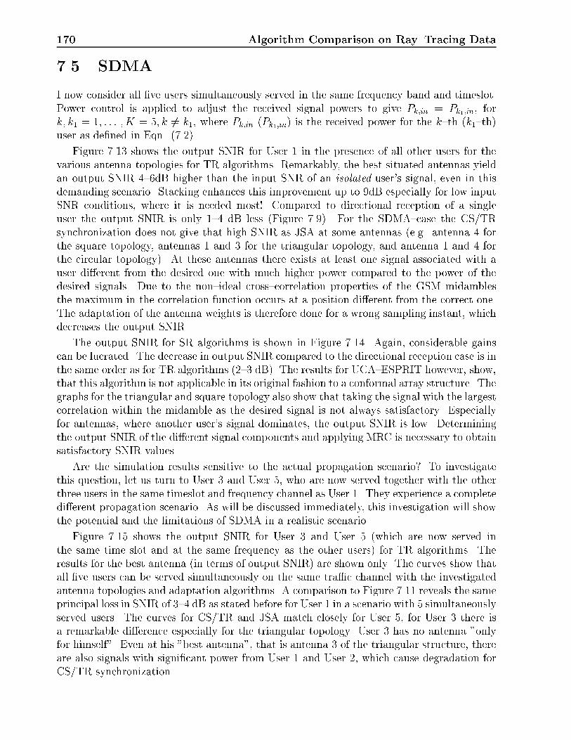
170 Algorithm Comparison on Ray{Tracing Data
7.5 SDMA
I now consider all �ve users simultaneously served in the same frequency band and timeslot.Power control is applied to adjust the received signal powers to give Pk;in = Pk1;in, fork; k1 = 1; : : : ; K = 5; k 6= k1, where Pk;in (Pk1;in) is the received power for the k{th (k1{th)user as de�ned in Eqn. (7.2).
Figure 7.13 shows the output SNIR for User 1 in the presence of all other users for thevarious antenna topologies for TR algorithms. Remarkably, the best situated antennas yieldan output SNIR 4{6dB higher than the input SNR of an isolated user's signal, even in thisdemanding scenario. Stacking enhances this improvement up to 9dB especially for low inputSNR conditions, where it is needed most! Compared to directional reception of a singleuser the output SNIR is only 1{4 dB less (Figure 7.9). For the SDMA{case the CS/TRsynchronization does not give that high SNIR as JSA at some antennas (e.g. antenna 4 forthe square topology, antennas 1 and 3 for the triangular topology, and antenna 1 and 4 forthe circular topology). At these antennas there exists at least one signal associated with auser di�erent from the desired one with much higher power compared to the power of thedesired signals. Due to the non{ideal cross{correlation properties of the GSM midamblesthe maximum in the correlation function occurs at a position di�erent from the correct one.The adaptation of the antenna weights is therefore done for a wrong sampling instant, whichdecreases the output SNIR.
The output SNIR for SR algorithms is shown in Figure 7.14. Again, considerable gainscan be lucrated. The decrease in output SNIR compared to the directional reception case is inthe same order as for TR algorithms (2{3 dB). The results for UCA{ESPRIT however, show,that this algorithm is not applicable in its original fashion to a conformal array structure. Thegraphs for the triangular and square topology also show that taking the signal with the largestcorrelation within the midamble as the desired signal is not always satisfactory. Especiallyfor antennas, where another user's signal dominates, the output SNIR is low. Determiningthe output SNIR of the di�erent signal components and applying MRC is necessary to obtainsatisfactory SNIR values.
Are the simulation results sensitive to the actual propagation scenario? To investigatethis question, let us turn to User 3 and User 5, who are now served together with the otherthree users in the same timeslot and frequency channel as User 1. They experience a completedi�erent propagation scenario. As will be discussed immediately, this investigation will showthe potential and the limitations of SDMA in a realistic scenario.
Figure 7.15 shows the output SNIR for User 3 and User 5 (which are now served inthe same time slot and at the same frequency as the other users) for TR algorithms. Theresults for the best antenna (in terms of output SNIR) are shown only. The curves show thatall �ve users can be served simultaneously on the same tra�c channel with the investigatedantenna topologies and adaptation algorithms. A comparison to Figure 7.11 reveals the sameprincipal loss in SNIR of 3{4 dB as stated before for User 1 in a scenario with 5 simultaneouslyserved users. The curves for CS/TR and JSA match closely for User 5, for User 3 there isa remarkable di�erence especially for the triangular topology. User 3 has no antenna "onlyfor himself". Even at his "best antenna", that is antenna 3 of the triangular structure, thereare also signals with signi�cant power from User 1 and User 2, which cause degradation forCS/TR synchronization.

7.5 SDMA 171
1
1 1
1
1 1
2
2 2
2
2 2
3
3 3
3
3 3
4 4
4 4
0
0 0
0
0 0
5
5 5
5
5 5
10
10 10
10
10 10
15
15 15
15
15 15
20
20 20
20
20 20
25
25 25
25
25 25
30
30 30
30
Antenna Nr.
Antenna Nr. Antenna Nr.
Antenna Nr.
Antenna Nr. Antenna Nr.
Out
put S
NIR
/dB
Out
put S
NIR
/dB
Out
put S
NIR
/dB
Out
put S
NIR
/dB
Out
put S
NIR
/dB
Out
put S
NIR
/dB
Input SNR/dB
Input SNR/dB Input SNR/dB
Input SNR/dB
Input SNR/dBInput SNR/dB
0
0
0
0
0
0
5
5
5
5
5
5
10
10
10
10
10
10
15
1515
15
15
15
20
2020
20
2020
(a) (b)
Squ
are
Topo
logy
Tria
ngul
ar T
opol
ogy
Circ
ular
Top
olog
y
Figure 7.13: Output SNIR for the three antenna topologies for a TR algorithm (LS), forUser 1 when all �ve users are served in the same timeslot and frequency channel (SDMA).(a) Horizontal linear array, (b) Quasi{planar array with four vertically stacked structures.|: JSA, o: CS/TR.

172 Algorithm Comparison on Ray{Tracing Data
1 1
1 1
2 2
2 2
3 3
3 3
4 40 0
0 0
0 0
5 5
5 5
10 10
1 1
10 10
15 15
15 15
20 20
5 5
20 20
25 25
25 25
Antenna Nr. Antenna Nr.
Input SNR/dB Input SNR/dB
Antenna Nr. Antenna Nr.
Out
put S
NIR
/dB
Out
put S
NIR
/dB
Out
put S
NIR
/dB
Out
put S
NIR
/dB
Out
put S
NIR
/dB
Out
put S
NIR
/dB
Input SNR/dB Input SNR/dB
Input SNR/dB Input SNR/dB
0
0
0
0
5
5
5
5
1010
10 10
15
15
1515
20
20
20 20
0 05 510 1015 1520 20
(a) (b)
Squ
are
Topo
logy
Tria
ngul
ar T
opol
ogy
Circ
ular
Top
olog
y
Figure 7.14: Output SNIR for the three antenna topologies for a SR algorithm (UnitaryESPRIT), for User 1 if all �ve users are served in the same timeslot and frequency channel(SDMA). (a) Horizontal linear array, (b) Quasi{planar array with four vertically stackedstructures. |: CS/SR, o: MRC.

7.5 SDMA 173
0 0
0 0
5 5
5 5
10 10
10 10
15 15
15 15
20 20
20 20
0 0
0 0
4 4
5 5
12 12
15 15
16 16
20 20
20 20
25 25
8 8
10 10
Out
put S
NIR
/dB
Out
put S
NIR
/dB
Out
put S
NIR
/dB
Out
put S
NIR
/dB
Input SNR/dB Input SNR/dB
Input SNR/dB Input SNR/dB
circularcircular
circular circular
square square
square
square
triangulartriangular
triangulartriangular
(a) (b)
Use
r 3
Use
r 5
Figure 7.15: Output SNIR versus the input SNIR for the best antenna for the di�erenttopologies for TR algorithms for User 3 and User 5, if all �ve users are served in the sametimeslot and frequency channel. (a) Horizontal linear array, (b) Quasi{planar array with fourvertically stacked structures. |: JSA, ��: CS/TR

174 Algorithm Comparison on Ray{Tracing Data
Figure 7.16 gives the results for User 3 and User 5 when applying an SR algorithm. All�ve users can be served simultaneously. The curves show a 1{4 dB decrease in output SNIRcompared to the directional reception case of Figure 7.11. Furthermore they show that MRC(or an SNIR criterion) is usually necessary to achieve the best possible output SNIR.
A comparison of TR and SR algorithms in terms of output SNIR shows that their perfor-mance for triangular and square topologies is nearly the same. TR algorithms with JSA givesometimes a higher output SNIR, but the di�erence is not tremendous. So I conclude thatSR algorithms perform in the same way or even better than TR algorithms with CS/TR.This is due to the non{ideal cross correlation properties of the GSM midambles.
7.6 Conclusions
This chapter analyzed the performance of various antenna topologies, synchronization strate-gies, and adaptation algorithms for directional reception and SDMA at a mobile communi-cations base station antenna.
My results show that any of the three antenna topologies performs nearly equal withTR adaptation algorithms. Since the aperture of all structures was nearly the same (20%di�erence maximum) I conclude that, for a certain aperture size, the physical details ofthe antenna do not really in uence the output SNIR. Stacking antennas vertically to forma quasi{planar array increases the output SNIR, especially for low{input SNR conditions,where it is needed most.
For the utilized conformal structure conventional SR algorithms like UCA{ESPRIT arenot suitable. They have to be modi�ed to include shadowing e�ects due to the antenna mast.
The adaptation strategies have to be always seen in conjunction with synchronization. ForTR algorithms CS/TR is usually not su�cient to reach the optimum SNIR for scenarios whereSDMA is used. For SR algorithms, where synchronization is done after DOA estimation andsignal reconstruction, i.e. on "clean" signals, a correlation{based synchronization methodalone is also not su�cient to achieve satisfactory performance. A criterion using the SNIR ofthe training sequences (midambles) of the di�erent reconstructed signals and an MRC, whichcan be realized for "nothing", since all information (time delays, output SNIRs) is readilyavailable, has to be implemented.
The performance in output SNIR of TR and SR algorithms is nearly the same. Due to thesynchronization issues considered above, SR algorithms have advantages for scenarios whereDOAs exist.
SR algorithms do not need any prior known data (training sequence) to estimate theDOAs and to reconstruct the incident signals, however, for the system and the detector toperform well at reasonable cost, a user identi�er, or, even better, a training sequence isneeded.
Systems that make optimal use of the angular distribution of the incoming signals, i.e.which utilize directional reception (and transmission) and/or SDMA, need better trainingsequences than used for GSM/DCS 1800. The sequences should have high autocorrelationand small cross{correlation, when they are in the complex baseband.
The adaptation schemes for the smart antenna do not cancel the ISI due to the mod-ulation (GMSK) and do not make use of the information about allowed transitions in the

7.6 Conclusions 175
0 0
00
5 5
55
10 10
1010
15 15
1515
20 20
2020
0 0
00
4 4
55
8 8
1010
12 12
1515
20 20
2525
16 16
2020
Out
put S
NIR
/dB
Out
put S
NIR
/dB
Out
put S
NIR
/dB
Out
put S
NIR
/dB
Input SNR/dB Input SNR/dB
Input SNR/dBInput SNR/dB
circular
square
triangular
circular
circularcircular
square
squaresquare
triangular
triangulartriangular
(a) (b)
Use
r 3
Use
r 5
Figure 7.16: Output SNIR versus the input SNIR for the best antenna for the di�erenttopologies for SR algorithms for User 3 and User 5, if all �ve users are served in the sametimeslot and frequency channel. (a) Horizontal linear array, (b) Quasi{planar array with fourvertically stacked structures. |: CS/SR, ��: MRC.

176 Algorithm Comparison on Ray{Tracing Data
signal{space diagram of the used modulation scheme. Furthermore, they cannot separateand optimally combine desired signals, which are incident from the same DOA (or within the3 dB{beamwidth of the reception antenna) just with a time delay. To accomplish for theseissues, an MLSE has to be implemented to process the output signals of the smart antennablock.
My investigations lead to the conclusion that the optimum receiver structure in termsof cost and performance is a SR scheme for DOA estimation and signal reconstruction, asynchronization circuit based on SNIR{values of the separated signals and a single{userMLSE (Viterbi detector), as it is used right now in GSM/DCS 1800, for optimal detection ofthe users signal. The MLSE needs only to have a short processing length of 3 bits maximum(the Gaussian transmit �lter for GSM introduces 2 bits of signi�cant ISI) just to eliminatethe ISI due to the modulation (e.g. GMSK) and to make use of the information about allowedtransitions in the signal{space diagram of the used modulation scheme.

Chapter 8
Downlink
This chapter gives some principal thoughts concerning downlink beamforming by using smartantennas. I will review the state{of{the{art, investigate a simple approach, and compare theresults for the downlink with the ones obtained for uplink processing for the same channelconstellation.
8.1 Basics
To obtain a capacity increase for a mobile communications system, smart antennas have tobe used both for the uplink and the downlink. While I have been focusing up to now onuplink processing only, I will here take a look on the downlink. Before proposing a suitablescheme I want to reemphasize the limits set by the duplex technique in conjunction with themobile radio channel and the system protocol.
The duplex technique has to be always considered in combination with the actual channelconstellation and the movement speed of the mobile. If the duplex technique is FDD, thesmall{scale fading on the uplink and the downlink for NLOS channels will be uncorrelated,as I have already shown in Chapter 2. Uncorrelated fading means that we cannot apply theantenna weights obtained from uplink processing directly for the downlink. If TDD is used,the fading appears strongly correlated for typical time delays between uplink and downlinktransmission [Big95].
Consider the following situation: Two users are subject to the same mean propagationloss. Due to the small{scale fading, however, the signal from one user (User 1) be 20dB belowthe one for the second user. The radiation pattern for reception of User 1 formed on theuplink will have a deep null into the direction of the incident signal belonging to User 2, toenable successful reception of the signal belonging to User 1. For User 2, however, the nullinto the direction of the signal from User 1 does not have to be that deep. This reveals animportant fact: The radiation pattern for the uplink is formed according to the instantaneouschannel constellation. If we determine the SNIRs for the two users, the one for User 1 willbe about 20dB below that for User 2.
� If we now reuse these patterns directly for the downlink of an FDD{system (like GSM)and compensate for the SNIR{di�erence, we may run into trouble. If we transmit 20dBmore power for User 1 than for User 2, we �ll up the null in the antenna pattern, whichis placed onto User 2, i.e. we decrease the receive SNIR of User 2.
177

178 Downlink
And in a real{world system we do not exactly know the location of the null and due toarray imperfections we cannot achieve in�nitely deep nulls.
In an NLOS situation the fading on the downlink frequency will be completely di�erentfrom that on the uplink frequency. If e.g. in the considered instantaneous situation atthe downlink both users su�er the same propagation loss, User 1 would have at leasta 20dB better SNIR than User 2, if the pattern null in the direction of User 1 in thepattern intended for transmission to User 2 is deep enough. A possible approach wouldbe not to compensate the SNIR di�erence and reuse the same antenna pattern.
� Since the uplink and downlink carrier frequencies are di�erent, the reuse of the antennaweights would result in a shift of the pattern maximum and the nulls, since with di�erentwavelengths for the up- and the downlink the antenna{dependent parameter d=� isdi�erent. A shift of the pattern maximum is rather unproblematic, since the maximumof the pattern is broad. The shift of the positions of the nulls is, however, problematic,since nulls are very steep, and a shift in only half of a degree in angle can causean attenuation di�erence for an undesired signal of some 10 dBs. Therefore for thedownlink the nulls have to be in exactly the same angular directions as for the uplink.
The next restriction is the necessity not to change the mobiles for today's mobile commu-nications systems. They should be as simple and cheap as possible, i.e. no interferencecancellation or sophisticated smart antenna processing unit should be implemented for low{cost mass{market products [Cal96]. But, antenna diversity might be one measure to improvethe performance of hand{helds.
This implies that we have to maximize the SNIR at the mobile by the pattern shape atthe BS to ensure a guaranteed reception quality. Only beamforming, i.e. a linear antennatype and structure can be utilized for the downlink. Therefore the downlink performance isdirectly related to the number of antenna elements M , i.e. the physical size of the antenna.The larger M , the larger the number of nulls that can be placed and the narrower the widthof the main beam. But, of course, the narrower the main beam, the larger the e�ect ofpointing errors.
8.2 Algorithm Types
Several algorithms have been proposed for downlink beamforming. Figure 8.1 gives anoverview of these approaches. I distinguish between linear and nonlinear algorithm typesfor adaptation of the transmission antenna weights. The reference is a purely spatial one,i.e. the antenna has to form a beam into a speci�c direction. As explained before, due tothe system requirements only linear antenna structures are suitable for the downlink. I willcharacterize the di�erent algorithms in the sequel.
8.2.1 Linear Algorithms
This group consists of all algorithms that do not make a nonlinear optimization of a prede�nedcriterion function.
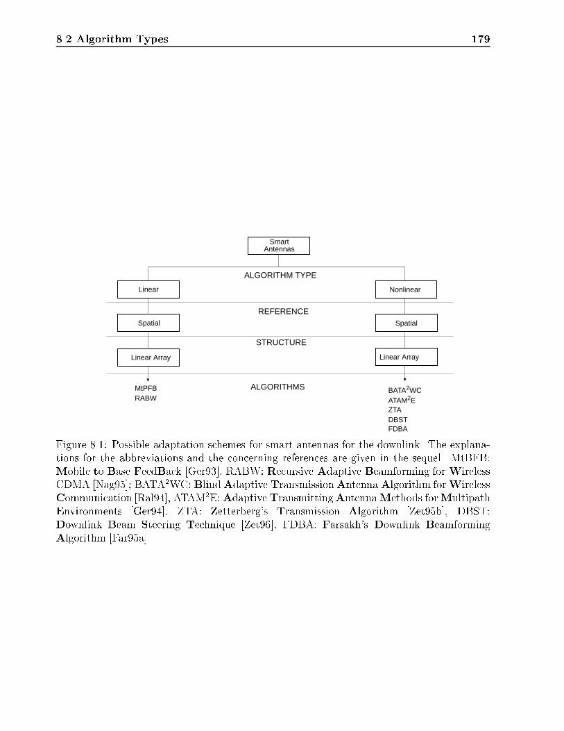
8.2 Algorithm Types 179
SmartAntennas
NonlinearLinear
Linear Array
Spatial Spatial
BATA2WCATAM2ERABW
MtPFB
Linear Array
ZTADBSTFDBA
ALGORITHM TYPE
ALGORITHMS
STRUCTURE
REFERENCE
Figure 8.1: Possible adaptation schemes for smart antennas for the downlink. The explana-tions for the abbreviations and the concerning references are given in the sequel. MtBFB:Mobile to Base FeedBack [Ger93], RABW: Recursive Adaptive Beamforming for WirelessCDMA [Nag95]; BATA2WC: BlindAdaptive TransmissionAntenna Algorithm forWirelessCommunication [Ral94], ATAM2E:Adaptive TransmittingAntennaMethods forMultipathEnvironments [Ger94], ZTA: Zetterberg's Transmission Algorithm [Zet95b], DBST:Downlink Beam Steering Technique [Zet96], FDBA: Farsakh's Downlink BeamformingAlgorithm [Far95a].

180 Downlink
� MtBFB (Mobile to Base FeedBack) [Ger93]: A probing tone is sent by the base(at the downlink frequency) for the purpose of channel impulse response measurementby the mobiles. These measurements are fed back to the base (closed loop). Fromthese measurements the channel impulse response matrixH(�; t) is determined and itshermitean transposed pseudoinverse is taken for the antenna weight vectors.
This method faces two important disadvantages: First, it needs a feedback loop, whichcan only be incorporated by making a change to the protocols in use. Second, sincethe instantaneous channel impulse response can change dramatically with only littlereceiver movement, the required feedback data rates are quite high.
� RABW (Recursive Adaptive Beamforming for Wireless CDMA) [Nag95]: The al-gorithm is based on the space{time array, which is called a 2D{RAKE structure inRef. [Nag95]. The array response vector of each path is estimated. Afterwards theseestimates have to be transferred to the downlink frequency.
Since in NLOS situations the small{scale fading is usually uncorrelated, this imposessevere problems.
8.2.2 Nonlinear Algorithms
For this class of algorithms a criterion is de�ned that is usually jointly optimized for all users.This can be done by any nonlinear optimization algorithm.
� BATA2WC (Blind Adaptive Transmission Antenna Algorithm forWireless Comm-unication) [Ral94]: This method forms a transmission beam pattern at the BS antennaarray (even for an FDD system) without any knowledge of the array geometry (onlythe arrays utilized for the uplink and the downlink should be similar), DOAs, or mobilefeedback.
Estimates of the receive vector channels are used to form a transmit weight vector opti-mization problem. A solution of this problem can be obtained by solving a generalizedeigenvalue problem.
� ATAM2E (Adaptive Transmitting Antenna Methods for Multipath Environments)[Ger94]: This algorithm is based on the observation that the scatterer's angular positionwith respect to the BS remains constant for rather long times and frequency separationsin the order of or larger than the duplex separation, as opposed to the fading structureof the channel, which varies rather rapidly.
The instantaneous vector channel is determined repeatedly while the MS moves. Thiscan be done by MtBFB. The vector channel uctuates due to MS motion, thereforethe channel vector will, on average, point into certain preferred directions and span thesubspace in which the channel vector roams. In contrast to the channel vector itself,this subspace is much more stable (the change in the DOAs is small). Exploiting thisfact reduces the feedback rates considerably.
Based on this assumption a set of independent optimization problems is derived | onefor each user. Again, the problem is reduced to a generalized eigenvalue problem thatcan be solved by the power method [Gol83].

8.3 Linear Algorithm for Antenna Weight Adjustment for the Downlink 181
� ZTA (Zetterberg's Transmission Algorithm) [Zet95b]: This algorithm determines theantenna weight vector wd;k for the k{th user in order to minimize the interference itcauses for other co{channel users. The required information is determined from thecovariance matrix derived from the data received at the uplink.
� DBST (Downlink Beam Steering Technique) [Zet96]: This technique is especiallysuited for GSM{like systems using SFIR. The training sequence of these systems isexplicitly made use of. As �rst step, the tap estimates of the impulse response on thereceive frequency (uplink) are obtained. With the observation that the array manifoldand the DOAs are about the same for the uplink and the downlink, and the assumptionthat the distribution of the impulse response in the transmit and in the receive modeshould be the same, a nonlinear criterion function is developed for maximizing thepower delivered to the desired MS. No care is taken about other MS's, therefore thealgorithm is only suited for range extension and SFIR applications.
� FDBA (Farsakh's Downlink BeamformingAlgorithm) [Far95a]: The criterion utilizedin Ref. [Far95a] is to minimize the ratio of useful power to interference power, i.e. theSIR (Signal to Interference Ratio), at the location of the users. These ratios aremaximized, which is again an eigenvalue problem.
The algorithm itself consists of two steps: First, the interference power is minimized,afterwards a linear or nonlinear improvement of the beamformer is performed.
8.3 Linear Algorithm for Antenna Weight Adjustment
for the Downlink
In this section I will present a purely linear adaptation algorithm for the antenna weights fordownlink transmission. It is suited for both FDD and TDD systems, since it utilizes onlyspatial (angular) properties of the mobile radio channel. I have divided this section into threeparts:
1. I will review the observations and assumptions necessary for downlink beamformingbased on information derived from the uplink.
2. I will show how the data for downlink beamforming are obtained from the uplink.
3. I will introduce a criterion function and demonstrate that it can be solved by linearprocessing. I will explain the beamforming algorithm and show some additional featuresthat can be easily incorporated into the system.
8.3.1 Observations and Assumptions Necessary for Downlink Beam-forming
In the following I will review the most important observations and assumptions, which haveto be taken into due consideration for downlink beamforming in GSM{like systems (wherethe main focus is on the FDD component) based on information obtained from the uplink.

182 Downlink
In the sequel, I will often make use of the word instantaneous. With this term I addressvalues for the DOAs and the associated SNIRs within one GSM timeslot.
� The fading of the uplink band and the downlink band is uncorrelated for NLOS situa-tions. This implies that instantaneous signal strengths (SNIRs) from the uplink cannotdirectly be made use of for the downlink. Only averaged (over a couple of timeslots)parameters are useful.
� The relative propagation loss for di�erent propagation paths is the same for the uplinkand the downlink. This assumption is justi�ed by the small relative duplex separation(GSM, DCS1800: �fduplex � 5%).
� The DOAs of the incident waves at the BS do not change remarkable (1) during severalbursts, and, (2) from the uplink to the downlink.
Assumption (1) is justi�ed by the spatial distance between BS and MS and the waytraveled by the MS during two consecutive timeslots. For instance, for vMS = 100km/h,the length of the path traveled by the MS during the reception of 10 consecutive times-lots is 1.28m. Even at a distance rMS = 100m between BS and MS the maximumchange in angle is 0:73�.
Assumption (2) is justi�ed by the duplex separation between up{ and downlink. Sinceit is rather small, the relevant re ectors will be the same both for the uplink and thedownlink.
� The DOAs are not discrete{valued. In most cases there is a nominal DOA associatedwith an angular spread.
With these observations and assumptions I will design a downlink beamforming algorithmthat is based on averaged quantities (DOAs and SNIRs) derived from the uplink. Thequantities necessary for the determination of the downlink radiation patterns are
� the DOAs of the incident signals associated with the user under consideration, and
� their SNIRs.
8.3.2 Determination of the Data Necessary for Downlink Beam-forming
To achieve reliable DOAs and SNIRs from the uplink, time averaging has to be done. Sincethe basis of my algorithm are DOAs, an SR algorithm has to be utilized with the uplinkdata to extract the desired quantities. This can be done within the uplink processing chain,or, if an approach di�erent from an SR algorithm is used for uplink processing, separatelyfor the downlink (see Figure 4.1, [Far96a]). The data derived from the SR algorithm is alsonecessary for channel allocation of the di�erent mobiles (see also Chapter 10).
Assume that K users are communicating with the BS of interest. Each of these Kusers has Lk; k = 1; 2; : : : ; K nominal DOAs. The word nominal means that all the localscattering is subsumed into one DOA. From the uplink results two matrices are produced |the uplink SNIR{matrix SNIRup and the uplink DOA{matrix DOAup. Both matrices are
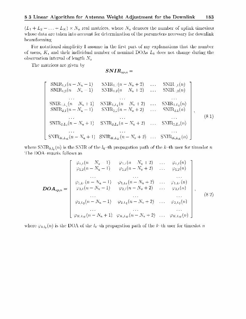
8.3 Linear Algorithm for Antenna Weight Adjustment for the Downlink 183
(L1 + L2 + : : : + LK) � Nu real matrices, where Nu denotes the number of uplink timeslotswhose data are taken into account for determination of the parameters necessary for downlinkbeamforming.
For notational simplicity I assume in the �rst part of my explanations that the numberof users, K, and their individual number of nominal DOAs Lk does not change during theobservation interval of length Nu.
The matrices are given bySNIRup;n =
2666666666666664
SNIR1;1(n�Nu + 1) SNIR1;1(n�Nu + 2) : : : SNIR1;1(n)SNIR1;2(n�Nu + 1) SNIR1;2(n�Nu + 2) : : : SNIR1;2(n)
: : : : : :. . . : : :
SNIR1;L1(n�Nu + 1) SNIR1;L1(n�Nu + 2) : : : SNIR1;L1(n)SNIR2;1(n�Nu + 1) SNIR2;1(n�Nu + 2) : : : SNIR2;1(n)
: : : : : :. . . : : :
SNIR2;L2(n�Nu + 1) SNIR2;L2(n�Nu + 2) : : : SNIR2;L2(n)
: : : : : :. . . : : :
SNIRK;LK(n�Nu + 1) SNIRK;LK(n�Nu + 2) : : : SNIRK;LK(n)
3777777777777775
;(8.1)
where SNIRk;lk(n) is the SNIR of the lk{th propagation path of the k{th user for timeslot n.The DOA{matrix follows as
DOAup;n =
2666666666666664
'1;1(n�Nu + 1) '1;1(n�Nu + 2) : : : '1;1(n)'1;2(n�Nu + 1) '1;2(n�Nu + 2) : : : '1;2(n)
: : : : : :. . . : : :
'1;L1(n�Nu + 1) '1;L1(n�Nu + 2) : : : '1;L1(n)'2;1(n�Nu + 1) '2;1(n�Nu + 2) : : : '2;1(n)
: : : : : :. . . : : :
'2;L2(n�Nu + 1) '2;L2(n�Nu + 2) : : : '2;L2(n)
: : : : : :. . . : : :
'K;LK(n�Nu + 1) 'K;LK(n�Nu + 2) : : : 'K;LK(n)
3777777777777775
;(8.2)
where 'k;lk(n) is the DOA of the lk{th propagation path of the k{th user for timeslot n.
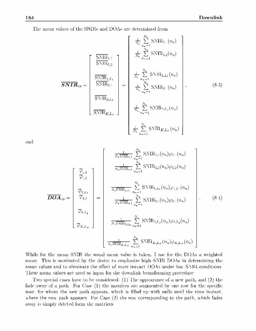
184 Downlink
The mean values of the SNIRs and DOAs are determined from
SNIRup =
2666666666666664
SNIR1;1
SNIR1;2...
SNIR1;L1
SNIR2;1...
SNIR2;L2...
SNIRK;LK
3777777777777775
=
26666666666666666666666666664
1Nu
NuPnu=1
SNIR1;1(nu)
1Nu
NuPnu=1
SNIR1;2(nu)
...
1Nu
NuPnu=1
SNIR1;L1(nu)
1Nu
NuPnu=1
SNIR2;1(nu)
...
1Nu
NuPnu=1
SNIR2;L2(nu)
...
1Nu
NuPnu=1
SNIRK;LK(nu)
37777777777777777777777777775
; (8.3)
and
DOAup =
2666666666666664
'1;1'1;1...
'1;L1'2;1...
'2;L2...
'K;LK
3777777777777775
=
26666666666666666666666666664
1NuSNIR1;1
NuPnu=1
SNIR1;1(nu)'1;1(nu)
1NuSNIR1;2
NuPnu=1
SNIR1;2(nu)'1;2(nu)
...
1NuSNIR1;L1
NuPnu=1
SNIR1;L1(nu)'1;L1(nu)
1NuSNIR2;1
NuPnu=1
SNIR2;1(nu)'2;1(nu)
...
1NuSNIR2;L2
NuPnu=1
SNIR2;L2(nu)'2;L2(nu)
...
1NuSNIRK;LK
NuPnu=1
SNIRK;LK(nu)'K;LK(nu)
37777777777777777777777777775
: (8.4)
While for the mean SNIR the usual mean value is taken, I use for the DOAs a weightedmean. This is motivated by the desire to emphasize high{SNIR DOAs in determining themean values and to eliminate the e�ect of more inexact DOAs under low{SNIR conditions.These mean values are used as input for the downlink beamforming procedure.
Two special cases have to be considered: (1) The appearance of a new path, and (2) thefade away of a path. For Case (1) the matrices are augmented by one row for the speci�cuser, for whom the new path appears, which is �lled up with nulls until the time instant,where the new path appears. For Case (2) the row corresponding to the path, which fadesaway is simply deleted form the matrices.

8.3 Linear Algorithm for Antenna Weight Adjustment for the Downlink 185
I calculate the mean values by applying a sliding rectangular window to the received data.One may question why I am not utilizing an exponential window, as it is done e.g. for theRLS{algorithm for channel tracking [Hay91] (by using a forgetting factor � < 1), thereforegiving more weight to the latest data and consecutively less weight to the older ones. Thereason for this is rather simple: I want to average out the small{scale fading. If I apply anexponential window and the actual data is derived from a channel condition with a fadingdip, a rather large weight is given to data, which is not that accurate as outside this dip (theolder data sets). Therefore the rectangular window is the natural choice.
8.3.2.1 Optimization Criterion
Before developing an algorithm for downlink beamforming, I want to establish a criterionto be optimized by the choice of the downlink weight vectors. The obvious criterion is tominimize the BER for the K mobiles jointly, therefore the most general criterion follows as
fwd;1;wd;2; : : : ;wd;k; : : : ;wd;Kg =
argfwd;1;wd;2;::: ;wd;k;::: ;wd;KgminfBER1;BER2; : : : ;BERk; : : : ;BERKg; (8.5)
where BERk is the bit error rate of the k{th user. The BER is a nonlinear function ofthe SNIR and therefore of the antenna weights. But, the BER increases with decreasingSNIR, therefore jointly maximizing the SNIRs for the mobiles gives an (maybe non{optimum)alternative criterion
fwd;1;wd;2; : : : ;wd;k; : : : ;wd;Kg =
argfwd;1;wd;2;::: ;wd;k;::: ;wd;KgmaxfSNIR1; SNIR2; : : : ; SNIRk; : : : ; SNIRKg;(8.6)
where SNIRk is the SNIR of the k{th user, which is given by
SNIRk =
LkPlk=1
wTd;krk;lk
2
�2k +KP
k1=1k1 6=k
LkPlk=1
wTd;krk;lk
2 ; (8.7)
where wd;k is the 1�M antenna weight vector for user k utilized for the downlink, �2k is thenoise power for the k{th user, and rk;lk is the steering vector for the lk{th propagation pathof the k{th user, given by
rk;lk = [1; ej2�d sin('k;lk )=�; : : : ; ej2k�d sin('k;lk )=�; : : : ; ej2(K�1)�d sin('k;lk )=�]T : (8.8)
For the derivation of the downlink beamforming algorithm I make two simplifying assump-tions that will be removed afterwards:
� Since no information about the angular spread of the signals is available, I assume theDOAs as discrete.

186 Downlink
� Since I also have no decisive information about the noise level for the various co{channel users, I assume the �ks as zero, i.e. I maximize the SIR. This assumption isalso motivated by the fact that cellular mobile communications systems are usuallyinterference limited.
With these assumptions we recognize that the SNIRk for the k{th user is maximized, ifall weight vectors fwd;1;wd;2; : : : ;wd;k1 ; : : : ;wd;Kg; k1 6= k lie in the space orthogonal to theone spanned by the weight vector wd;k for the k{th user,
fwd;1;wd;2; : : : ;wd;k1; : : : ;wd;Kg; k1 6= k ? wd;k: (8.9)
In that case there is no interference for User k, only the desired signal is present (i.e. SNIR!1).
Since the above argument for maximization of the SNIR at the mobile holds true for allusers, I arrive at the conclusion that any two weight vectors have to be orthogonal,
wd;k1 ? wd;k 8k1; k with k1 6= k: (8.10)
Under the assumption L1 + L2 + : : : + LK < M this criterion can be ful�lled with a purelylinear algorithm, which starts from the same basis as the signal reconstruction algorithm usedfor SR algorithms.
8.3.3 Downlink Beamforming Algorithm
I will introduce two algorithms for beamforming | the WSA (Weight and Sum Algorithm)and the SWA (Sum and Weight Algorithm). The di�erence lies in the way they handledi�erent paths belonging to one MS.
WSA consists of the following steps:
1. Calculate the downlink array steering matrix
Adown = [a('1;1);a('1;2); : : : ;a('1;L1);a('1;2); : : : ;a('2;L2); : : : ;a('K;LK)](8.11)
with
a('k;lk) = [1; e�j2�d sin('k;lk )=�d ; : : : ; e�j2�(M�1)d sin('k;lk )=�d ]T ; (8.12)
where �d is the wavelength at the downlink frequency.
2. Determine the Moore{Penrose pseudoinverse of Adown as
W down =
26666666666664
wd;1;1
wd;1;2...
wd;1;L1...
wd;2;L2...
wd;K;LK
37777777777775= A+
down; (8.13)

8.3 Linear Algorithm for Antenna Weight Adjustment for the Downlink 187
which contains the desired antenna weight vector for each propagation path.
This follows since the product
W downAdown = IL1+L2+:::+LK (8.14)
is the (L1 + L2 + : : :+ LK)� (L1 + L2 + : : :+ LK) identity matrix, i.e. the product ofthe rows of W down and the columns of Adown with equal numbers are equal to unity,those with non-equal numbers are equal to zero.
Afterwards, the K downlink weight vectors are formed by
W d =
26664wd;1
wd;2...
wd;K
37775 =
26666666664
L1Pl1=1
wd;1;l1
L2Pl2=1
wd;2;l2
...LKPlK=1
wd;K;lK
37777777775: (8.15)
SWA di�ers from WSA as follows:
1. Perform the same operations as in Step 1 for the �rst algorithm, however, construct amodi�ed array steering matrix by
~Adown =
"1
L1
L1Xl1=1
a('1;l1);1
L2
L2Xl2=1
a('2;l2); : : : ;1
LK
LKXlK=1
a('K;lK)
#:
(8.16)
This means that I group the DOAs belonging to one user before determining the down-link weight vector.
2. Now, the pseudoinverse of this new steering matrix
~W d = ~W down =
26664
~wd;1
~wd;2...
~wd;K
37775 = A+
down; (8.17)
is taken as the matrix of the antenna weights.
I do not compensate for the SNIR{di�erence for di�erent users. The reason for that isexplained in more detail in Chapter 10.
Figure 8.2a shows the downlink antenna patterns for a scenarios with three users locatedat '1 = �30�, '2 = 0�, and '3 = 40�, measured from array broadside. The deep nulls ofthe pattern for a speci�c user into the directions of the other users can be clearly seen. ForFigure 8.2b and 8.2c it is assumed that the DOAs '1 = '1;1 = �30� and '3 = '1;2 = 40�
correspond to one user. Figure 8.2b shows the patterns derived by using WSA (adding the

188 Downlink
0
0 0
-10
-10 -10
-20
-20 -20
-30
-30 -30
-40
-40 -40
-50
-50 -50
-10
-10 -10
10
10 10
50
50 50
90
90 90
-50
-50 -50
-90
-90 -90
Ant
enna
gai
n (d
B)
Ant
enna
gai
n (d
B)
Ant
enna
gai
n (d
B)
ϕ/deg.
ϕ/deg. ϕ/deg.
ϕ1,1
ϕ1 ϕ1,1
ϕ2
ϕ2 ϕ2
ϕ1,2
ϕ3 ϕ1,2
(a) (b)
(c)
3 Users 2 UsersWSA
2 UsersSWA
User 1 User 1
User 1
User 2 User 2
User 2
User 3 User 1
User 1
Figure 8.2: Downlink radiation patterns. (a) Patterns for three users located at '1 = �30�,'2 = 0�, and '3 = 40�. For (b) and (c) the DOAs '1 = '1;1 = �30� and '3 = '1;2 = 40�
correspond to one user. (b) Radiation patterns derived by WSA. (c) Radiation patternsderived by SWA.

8.3 Linear Algorithm for Antenna Weight Adjustment for the Downlink 189
individual patterns from Figure 8.2a. The nulls of the pattern for the second user (DOA'2 = 0�) are, of course, still into the directions of the DOAs for the (now) �rst user.
Figure 8.2c shows the patterns derived by applying SWA. The locations of the patternnulls for the second user do not exactly point anymore into the directions of the DOAs forthe �rst user. Therefore WSA is favored for application purposes. However, in real{worldsystems the nulls are not in�nitely deep due to imperfect calibration and environment e�ects.Therefore the | computationally cheaper | SWA should not be ruled out completely.
I now come back to the two simplifying assumptions I have made for the derivation of thealgorithm. Let me start with the second one, where I have assumed discrete{valued DOAs.But, in reality there is a certain angular spread associated with each DOA.
To take this e�ect into account the null broadening algorithm of [Ger96] is implemented.The details of this approach are shown in Appendix G. Note that this approach necessi-tates the determination of the antenna pattern for each user separately, since the alteredarray steering matrix Adown;k;lk, the matrix containing the conditions for the null broadeningalgorithm, F k;lk , and the projection matrix Dk;lk are di�erent for each path (for detailedexplanation of these quantities see Appendix G). Figures 8.3a and 8.3c again show the radia-tion pattern for the three users located at '1 = �30�, '2 = 0�, and '3 = 40�. But, in Figure8.3a the null broadening parameter was set to PNB = 1 (i.e. the �rst order derivatives at thenulls are set to zero) and in 8.3c to PNB = 2 (the second order derivatives are set to zero).The nulls are indeed remarkably broader. However, also the main beam starts to broadenand the sidelobe level increases. This e�ect can be seen in particular in Figure 8.3c for theDOAs far from antenna broadside. Figures 8.3b and 8.3d show the patterns for consideringthe DOAs '1 = '1;1 = �30� and '3 = '1;2 = 40� belonging to User 1. Again the deep nullsand the larger sidelobe level can be seen (compare to Figure 8.2).
The fact that I maximize the SIR instead of the SNIR, i.e. I neglect the unknown noisecontribution at the MS position, leads to problems especially for poorly spatially separablescenarios. The channel allocation algorithm has to take care for these e�ects, so that scenarioswith poor spatial separability are ruled out beforehand.
Usually the propagation paths belonging to di�erent DOAs 'k;lk are di�erent [Kle96b].Since the proposed algorithms only form a beam into the directions to be transmitted, theydo not compensate for the propagation delays. This is not necessary, since the MS (forGSM{like systems) has an equalizer, which bene�ts from these delayed paths [DAr91].
Without restriction of generality assume that two signi�cant propagation paths existbetween the MS and the BS. Both be subjected to the same mean propagation loss. Theshort{term uctuation of the transmission loss be Rayleigh distributed [Jak74]. Thereforethe BER for a MSK{modulated signal with MRC (there are two independent paths perassumption) follows as (see also Appendix C)
hBERiMRC =1
2
1� �(6 + 2�)p
2(2 + �)p2�(2 + �)
!(8.18)
and for selection diversity as
hBERisel = 1
2
1� 2
r�
� + 2+
r�
� + 4
!; (8.19)

190 Downlink
0
0
0
0
-10
-10
-10
-10
-20
-20
-20
-20
-30
-30
-30
-30
-40
-40
-40
-40
-50
-50
-50
-50
-10
-10
-10
-10
10
10
10
10
50
50
50
50
90
90
90
90
-50
-50
-50
-50
-90
-90
-90
-90
Ant
enna
gai
n (d
B)
Ant
enna
gai
n (d
B)
Ant
enna
gai
n (d
B)
Ant
enna
gai
n (d
B)
ϕ/deg.
ϕ/deg.
ϕ/deg.
ϕ/deg.
ϕ1
ϕ1
ϕ1,1
ϕ1,1
ϕ2
ϕ2
ϕ2
ϕ2
ϕ3
ϕ3
ϕ1,2
ϕ1,2
(a) (b)
(c) (d)
2 Users
2 Users
3 Users
3 Users
WSA, first order derivatives set to zero
WSA, first and second order derivatives set to zeroUser 1
User 1
User 1
User 1
User 2
User 2
User 2
User 2
User 1
User 1
User 3
User 3
Figure 8.3: Downlink radiation patterns. (a) Patterns for three users located at '1 = �30�,'2 = 0�, and '3 = 40� with the null broadening parameter PNB = 1. For (b) and (d)the DOAs '1 = '1;1 = �30� and '3 = '1;2 = 40� correspond to one user. (b) Radiationpatterns derived by WSA with the null broadening parameter PNB = 1, i.e. the �rst orderderivative at the nulls is set to zero. (c) Radiation patterns from (a) with the null broadeningparameter PNB = 2, i.e. the �rst and the second order derivative at the null are set to zero.(d) Radiation patterns from (b) with the null broadening parameter PNB = 2.
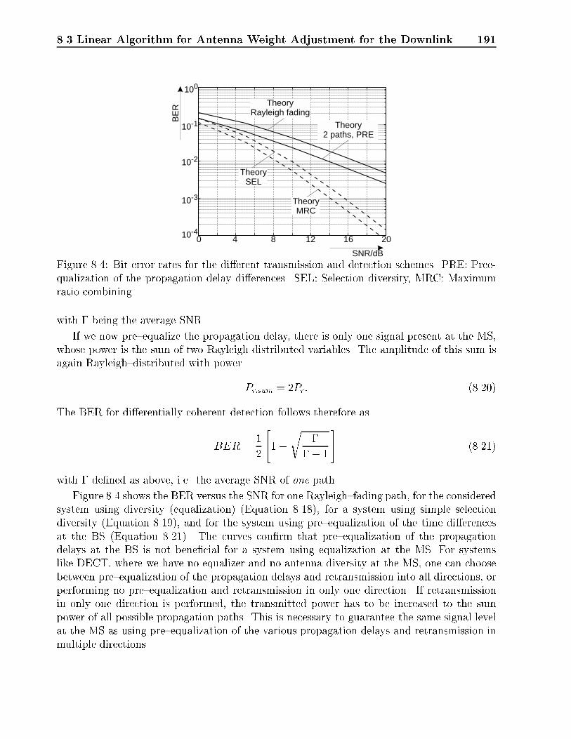
8.3 Linear Algorithm for Antenna Weight Adjustment for the Downlink 191
100
10-3
10-2
10-4
10-1
4 12 168 200
SNR/dB
BE
R
Theory2 paths, PRE
TheoryRayleigh fading
TheorySEL
TheoryMRC
Figure 8.4: Bit error rates for the di�erent transmission and detection schemes. PRE: Pree-qualization of the propagation delay di�erences. SEL: Selection diversity, MRC: Maximumratio combining.
with � being the average SNR.
If we now pre{equalize the propagation delay, there is only one signal present at the MS,whose power is the sum of two Rayleigh distributed variables. The amplitude of this sum isagain Rayleigh{distributed with power
Pr;sum = 2Pr: (8.20)
The BER for di�erentially coherent detection follows therefore as
BER =1
2
"1�
r�
� + 1
#(8.21)
with � de�ned as above, i.e. the average SNR of one path.
Figure 8.4 shows the BER versus the SNR for one Rayleigh{fading path, for the consideredsystem using diversity (equalization) (Equation 8.18), for a system using simple selectiondiversity (Equation 8.19), and for the system using pre{equalization of the time di�erencesat the BS (Equation 8.21). The curves con�rm that pre{equalization of the propagationdelays at the BS is not bene�cial for a system using equalization at the MS. For systemslike DECT, where we have no equalizer and no antenna diversity at the MS, one can choosebetween pre{equalization of the propagation delays and retransmission into all directions, orperforming no pre{equalization and retransmission in only one direction. If retransmissionin only one direction is performed, the transmitted power has to be increased to the sumpower of all possible propagation paths. This is necessary to guarantee the same signal levelat the MS as using pre{equalization of the various propagation delays and retransmission inmultiple directions.

192 Downlink
8.4 Performance Analysis
This section gives the results of a performance analysis of WSA. Two users are supportedin an SDMA mode. The channel model is the low{rank channel (local scatterer model) asalready used in Chapter 6, i.e. there is one group of scatterers around the MS. To takethe time behavior of the mobile radio channel into account, the moving scatterer model wasimplemented (Chapter 2). As start of a simulation run a scenario was determined, wherethe minimum angular distance between the two users was set to �'DOA = 30� to guaranteeseparability. Then, Nu simulations were run with the moving scatterer model. The choice ofthe parameter Nu is in uenced by two system{dependent constraints:
� The averaging period should be long enough to average out the Rayleigh fading of thechannel.
� On the other hand, the averaging period should be short enough not to average out thelong{term fading.
I chose a value of Nu = 20 timeslots for the size of the averaging window. This is a reasonablevalue (Recently Ref. [Zet96] used Nu = 21).
The radius of the local scatterer circle was set to R = 200�. The distance between theMS and the BS was assumed as �xed; the values are given separately for each simulationblock.
The antenna was anM = 8{element 1D{ULA with d=�d = 0:5 for the downlink frequency(d=� = 0:476 for the uplink).
The SNIR at the BS and at the MS's were determined from the data �elds of the GSM{timeslot for comparison purposes. For proper operation of the GSM{system an SNIR of atleast 9dB is necessary. Since the simulation takes into account the small{scale fading, I donot have to add any small{scale fading margin. I choose a threshold value of SNIRth = 10dBfor comparison of the approaches.
8.4.1 Immediate Weight Reuse
Figure 8.5 shows the CDFs of the output SNIRs for immediate reuse of the antenna weightsdetermined at the uplink (Nu = 1). The distance between the MS and the BS was set torMS = 10000�.
For an input SNR of 30dB on the uplink the output SNIR is in less than 1% of the casesless than SNIRth (Figure 8.5a). The SNIR curves show that an instantaneous weight reusedoes not give acceptable results. For an input SNR of 30dB on the downlink the outputSNIR is less than SNIRth in 73% (82%) of the cases for reusing the weights determined bythe application of Unitary Esprit (LS) (Figures 8.5b, 8.5c).
However, if the ideally known DOAs and SNIRs are utilized as input for the downlinkbeamforming algorithm, promising results are obtained. For an input SNR of 30dB on thedownlink the output SNIR is in only 1% of the cases less than the threshold, SNIRth (Figures8.5b and 8.5c).
Figure 8.6 shows the same principal results for a reuse of the uplink weights after Nu = 20iterations. The results behave like the ones with immediate weight reuse, which shows that

8.4 Performance Analysis 193
0
0 0
0.2
0.2 0.2
0.4
0.4 0.4
0.6
0.6 0.6
0.8
0.8 0.8
1
1 1
0
0 0
10
10 10
20
20 20
30
30 30
40
40 40
SNR=10dB
SNR=10dB SNR=10dB
SNR=30dB
SNR=30dB SNR=30dB
SNR=20dB
SNR=20dB SNR=20dB
SNR=0dB
SNR=0dBSNR=0dB
CD
F(O
utpu
t SN
IR)
CD
F(O
utpu
t SN
IR)
CD
F(O
utpu
t SN
IR)
Output SNIR (dB)
Output SNIR (dB) Output SNIR (dB)
(a)
(b) (c)
Immediate weight reuse
Uplink
DownlinkSR algorithm (Unitary ESPRIT)
DownlinkTR algorithm (LS)
Figure 8.5: CDFs of the output SNIRs with immediate reuse of the weights from the uplinkwith the input SNR as parameter. Distance between BS and MS, rMS = 10000�. |: UnitaryESPRIT, � ��: LS, grey curve: Downlink beamforming based on ideal DOAs and SNIRs;(a) Uplink SNIRs; (b) Downlink SNIRs with the weights determined by Unitary ESPRIT;(c) Downlink SNIRs with the weights determined by LS.

194 Downlink
(a)
(b) (c)
0
0 0
0.2
0.2 0.2
0.4
0.4 0.4
0.6
0.6 0.6
0.8
0.8 0.8
1
1 1
0
0 0
10
10 10
20
20 20
30
30 30
40
40 40
SNR=10dB
SNR=10dB SNR=10dB
SNR=30dB
SNR=30dB SNR=30dB
SNR=20dB
SNR=20dB SNR=20dB
SNR=0dB
SNR=0dB
SNR=0dB
CD
F(O
utpu
t SN
IR)
CD
F(O
utpu
t SN
IR)
CD
F(O
utpu
t SN
IR)
Output SNIR (dB)
Output SNIR (dB) Output SNIR (dB)
Weight reuse after Nu=20 iterations
Uplink
DownlinkSR algorithm (Unitary ESPRIT)
DownlinkTR algorithm (LS)
Figure 8.6: CDFs of the output SNIRs with the reuse of the weights from the uplink afterNu = 20 iterations with the input SNR as parameter. Distance between BS and MS, rMS =10000�. |: Unitary ESPRIT, ���: LS, grey curve: Downlink beamforming based on idealDOAs and SNIRs; (a) Uplink SNIRs; (b) Downlink SNIRs with the weights determined byUnitary ESPRIT; (c) Downlink SNIRs with the weights determined by LS.

8.4 Performance Analysis 195
weight reuse is not the way to proceed. The estimated DOAs are subjected to a large standarddeviation, since there is a �nite angular spread (see also Chapter 5). Whereas this e�ect onlyslightly impairs the reception of the wanted signal (since the main beam is rather broad, soa standard deviation in angle of a few degrees is not that critical), it signi�cantly a�ects thenulls. Since for each timeslot the nulls are usually at slightly di�erent positions, they aree�ectively �lled up and therefore one produces more interference into undesired directions.
8.4.2 Reuse of DOAs and SNIRs from the Uplink
Figure 8.7 shows the CDFs of the output SNIRs with the reuse of the uplink DOAs andSNIRs. The distance between BS and MS was set to rMS = 10000�.
Since TR algorithms do not give DOAs directly, the maxima of the antenna patterns forthe speci�c users are interpreted as the DOAs of the desired signals and afterwards the sameprocedure as for SR algorithms is used.
For an input SNR of 30dB on the uplink the output SNIR is in less than 1% of thecases less than SNIRth (Figure 8.7a). With ideally known DOAs and SNIRs as input to thedownlink beamforming algorithm the output SNIR at the MS is in 5% of the cases less thanSNIRth (Figures 8.7b and 8.7c).
A use of the uplink DOAs and SNIRs determined by Unitary ESPRIT results in anoutput SNIR at the mobile, which is in 15% less than the threshold, SNIRth (Figure 8.7b)The reuse of the pattern maxima for TR algorithms results in satisfactory performance forlow{SNR (SNR < 20dB) scenarios, for high{SNR scenarios (SNR � 20dB) the performancesigni�cantly degrades (the output SNIR is less than the threshold, SNIRth, in 59% of thecases for an input SNR of 30dB (Figure 8.7c). The reason for this somewhat surprising e�ecthas been already explained in Chapter 5. The problem TR approaches face at high input{SNR conditions is the illconditioned covariance matrix used for determining the weights. Foran input SNR > 20dB the standard deviation of the DOA derived from the maximum of theantenna pattern increases with increasing SNR (see Chapter 5). Therefore the reuse of themaxima results in non{satisfactory behavior for input SNRs in excess of 20 dB.
In the next section I will be looking on broad nulls. They are e�ective against estimationerrors of the null position and against large angular spreads. These large angular spreadsoccur, if the distance between MS and BA, rMS, is rather low. Therefore I also analyze in thissection the performance of the algorithms for a distance between MS and BS, rMS = 1500�.Figure 8.8 shows the CDFs of the output SNIRs with the reuse of the uplink DOAs andSNIRs. Basically nothing changes to the results of Figure 8.7.
8.4.3 Broad Nulls
Figure 8.9 shows the CDFs of the output SNIRs with and without application of the nullbroadening algorithm for the DOAs and SNIRs determined by Unitary ESPRIT, for rMS =1500�.
For an input SNR of 30dB on the uplink the output SNIR is in less than 1% of the casesless than SNIRth (Figure 8.9a).
In Figure 8.9b the ideal curves and the results obtained by simply reusing the DOAswithout any null broadening are shown. For an input SNR of 30dB the output SNIR at

196 Downlink
(a)
(b) (c)
0
0 0
0.2
0.2 0.2
0.4
0.4 0.4
0.6
0.6 0.6
0.8
0.8 0.8
1
1 1
0
0 0
10
10 10
20
20 20
30
30 30
40
40 40
SNR=10dB
SNR=10dB
SNR=10dB
SNR=30dB
SNR=30dB SNR=30dB
SNR=20dB
SNR=20dBSNR=20dB
SNR=0dB
SNR=0dB
SNR=0dB
CD
F(O
utpu
t SN
IR)
CD
F(O
utpu
t SN
IR)
CD
F(O
utpu
t SN
IR)
Output SNIR (dB)
Output SNIR (dB) Output SNIR (dB)
DOA/SNIR reuse
Uplink
DownlinkSR algorithm (Unitary ESPRIT)
DownlinkTR algorithm (LS)
Figure 8.7: CDFs of the output SNIRs with the use of the uplink DOAs and SNIRs with anobservation interval of length Nu = 20 and the input SNR as parameter. Distance betweenBS and MS, rMS = 10000�. |: Unitary ESPRIT, � � �: LS, grey curve: Downlinkbeamforming based on ideal DOAs and SNIRs; (a) Uplink SNIRs; (b) Downlink SNIRs withDOAs and SNIRs determined by Unitary ESPRIT; (c) Downlink SNIRs with DOAs andSNIRs determined by LS.

8.4 Performance Analysis 197
(a)
(b) (c)
0
0 0
0.2
0.2 0.2
0.4
0.4 0.4
0.6
0.6 0.6
0.8
0.8 0.8
1
1 1
0
0 0
10
10 10
20
20 20
30
30 30
40
40 40
SNR=10dB
SNR=10dBSNR=10dB
SNR=30dB
SNR=30dBSNR=30dB
SNR=20dB
SNR=20dB SNR=20dB
SNR=0dB
SNR=0dB
SNR=0dB
CD
F(O
utpu
t SN
IR)
CD
F(O
utpu
t SN
IR)
CD
F(O
utpu
t SN
IR)
Output SNIR (dB)
Output SNIR (dB) Output SNIR (dB)
DOA/SNIR reuse
Uplink
DownlinkSR algorithm (Unitary ESPRIT)
DownlinkTR algorithm (LS)
Figure 8.8: CDFs of the output SNIRs with the use of the uplink DOAs and SNIRs withan observation interval of length Nu = 20 and the input SNR as parameter. Distancebetween BS and MS, rMS = 1500�. |: Unitary ESPRIT, ���: LS, grey curve: Downlinkbeamforming based on ideal DOAs and SNIRs; (a) Uplink SNIRs; (b) Downlink SNIRs withDOAs and SNIRs determined by Unitary ESPRIT; (c) Downlink SNIRs with DOAs andSNIRs determined by LS.

198 Downlink
(a)
(b) (c)
0
0 0
0.2
0.2 0.2
0.4
0.4 0.4
0.6
0.6 0.6
0.8
0.8 0.8
1
1 1
0
0 0
10
10 10
20
20 20
30
30 30
40
40 40
SNR=10dB
SNR=10dB SNR=10dB
SNR=30dB
SNR=30dBSNR=30dB
SNR=20dB
SNR=20dB SNR=20dB
SNR=0dB
SNR=0dBSNR=0dB
CD
F(O
utpu
t SN
IR)
CD
F(O
utpu
t SN
IR)
CD
F(O
utpu
t SN
IR)
Output SNIR (dB)
Output SNIR (dB) Output SNIR (dB)
DOA/SNIR reuse & null broadeningUplink
Downlink DownlinkSR algorithm without null broadeningideal DOAs without null broadening
SR algorithm with null broadeningideal DOAs without null broadening
Figure 8.9: CDFs of the output SNIRs with the DOAs and SNIRs derived from the uplinkwith an observation interval of length Nu = 20 and the input SNR as parameter. The nullbroadening algorithm with PNB = 1 (�rst order derivatives at the nulls set to zero) is testedagainst the scheme without null broadening. Distance between BS and MS, rMS = 1500�. |:Unitary ESPRIT, � � �: LS, grey curve: Downlink beamforming without null broadeningbased on ideal DOAs and SNIRs; (a) Uplink SNIRs; (b) Downlink SNIRs, beamformingwithout null broadening for DOAs and SNIRs determined by Unitary ESPRIT, beamformingwithout null broadening for ideal DOAs and SNIRs; (c) Downlink SNIRs, beamforming withnull broadening for DOAs and SNIRs determined by Unitary ESPRIT, beamforming withoutnull broadening for ideal DOAs and SNIRs.

8.5 Conclusions 199
the downlink is in 8% (13%) of the cases less than the threshold, SNIRth, for the use of theideal weights (weights determined by Unitary ESPRIT at the uplink). One loses about 4dBin output SNIR by reusing the DOAs from the uplink compared to downlink beamformingbased on the ideal DOAs.
Figure 8.9c shows the results obtained by applying the null broadening algorithm withPNB = 1 (only the �rst{order derivatives are set to zero) to the data from the uplink. Foran input SNR of 30dB the output SNIR at the downlink is in 8% of the cases less than thethreshold value, SNIRth, with the weights determined from the DOAs and SNIRs derivedby applying Unitary ESPRIT at the uplink. Especially for the high input SNR and smalloutput SNIR region the null broadening algorithm outperforms the algorithm using the usualpattern.
Figure 8.10 shows the CDFs of the output SNIRs with and without application of thenull broadening algorithm to the ideal DOAs for rMS = 10000�. They show that additionalimprovement can be lucrated by applying the null broadening algorithm also to beamformingbased on ideal DOAs. Without null broadening for an input SNR of 30dB the output SNIR atthe downlink would be below the threshold in 4% of the cases, whereas with null broadeningthis value is reduced to 1%.
By using the null broadening algorithm the performance of the downlink is decisivelyincreased for well separable scenarios compared to an algorithm utilizing only the conventionalantenna pattern.
In summary, all �gures show that the downlink output SNIR is below the one at theuplink. Additionally at the downlink a larger gradient of the curves especially for the lowoutput SNIR region exists, which results in higher BERs.
8.5 Conclusions
This chapter analyzed the challenging scenario for the downlink in FDD systems and com-pared it to the uplink. I proposed a linear downlink beamforming algorithm suitable for bothTDD and FDD systems. It reuses DOAs and the corresponding SNIRs derived by an SRalgorithm on the uplink.
The results indicate that the downlink is the bottleneck. The SNIR is about 2{4dB belowthe one obtained from the uplink. Beamforming can only be done on time{averaged values(DOAs, SNIRs) derived from the uplink, while the uplink processing scheme works on theinstantaneous channel constellation, which improves its performance.
DOAs derived from the maximum of the antenna pattern adjusted by a TR algorithmare not really suitable for the downlink. One approach to remedy this shortcoming of TRalgorithms would be to reuse only the nulls of the pattern | they should be in the directionsof the interfering signals | and not to take care about the maximum. However, in this senseTR algorithms do not give any information valuable for channel allocation (which DOAcorresponds to which user) | an SR algorithm (i.e. DOAs) is still needed. The DOAs andSNIRs derived from SR algorithms applied to the uplink data provide a promising startingpoint for downlink beamforming.
Null broadening is a promising scheme. It increases the output SNIR by about 3dBespecially in the low output{SNIR region, where it is needed most.

200 Downlink
(a)
(b) (c)
0
0 0
0.2
0.2 0.2
0.4
0.4 0.4
0.6
0.6 0.6
0.8
0.8 0.8
1
1 1
0
0 0
10
10 10
20
20 20
30
30 30
40
40 40
SNR=10dB
SNR=10dB SNR=10dB
SNR=30dB
SNR=30dB SNR=30dB
SNR=20dB
SNR=20dB
SNR=20dB
SNR=0dB
SNR=0dB SNR=0dB
CD
F(O
utpu
t SN
IR)
CD
F(O
utpu
t SN
IR)
CD
F(O
utpu
t SN
IR)
Output SNIR (dB)
Output SNIR (dB) Output SNIR (dB)
DOA/SNIR reuse & null broadening
Uplink
Downlink DownlinkSR algorithm without null broadeningideal DOAs without null broadening
SR algorithm without null broadeningideal DOAs with null broadening
Figure 8.10: CDFs of the output SNIRs with the DOAs and SNIRs derived from the uplinkwith an observation interval of length Nu = 20 and the input SNR as parameter. The nullbroadening algorithm with PNB = 1 (�rst order derivatives at the nulls set to zero) is testedagainst the scheme without null broadening. Distance between BS and MS, rMS = 10000�.|: Unitary ESPRIT, ���: LS, grey curve: Downlink beamforming based on ideal DOAsand SNIRs; (a) Uplink SNIRs; (b) Downlink SNIRs, beamforming without null broadeningfor DOAs and SNIRs determined by Unitary ESPRIT, beamforming without null broadeningfor i deal DOAs and SNIRs; (c) Downlink SNIRs, beamforming without null broadening forDOAs and SNIRs determined by Unitary ESPRIT, beamforming with null broadening foride al DOAs and SNIRs.
8.5 Conclusions 201
Pre{equalization of the propagation delays at the BS, as proposed in Ref. [Slo95], doesnot increase link performance. If an equalizer or antenna diversity is used at the MS, theperformance even degrades. But, parts of the problems concerning the downlink can berelaxed by simply increasing the transmit power, which poses no essential problem for theBSs. A further measure to increase link quality is the use of antenna diversity at the MS, asproposed e.g. in [Yam91] and [Fuh95c].
I see my results just as a �rst step. Further algorithm re�nement for the downlink has tobe made in order to fully assess its potential.


Chapter 9
Capacity Enhancement
The chapters up to now have focused on channel modeling, signal processing aspects, andperformance assessment of algorithms for smart antennas. Here, I try to give an impressionof the potential capacity increase achievable by this technology. I will analyze both SFIR andSDMA and compare them to a conventional system using omnidirectional or sector antennas.
To make a meaningful comparison of the di�erent systems, a simulation tool for deter-mination of the CIR (Carrier to Interference Ratio) in a multicell scenario was developed.Some features of this software are inspired by the simulation tool presented in Ref. [Tsou96].
There are a number of estimates for the capacity increase already available in literature.Ref. [Swa90] analyzed the performance enhancement of multibeam adaptive BS antennas.A comparison between an adaptive antenna capable of forming eight beams and an omni-directional antenna showed that the former could provide a threefold increase in spectrale�ciency.
Ref. [Tan94] determined the gain in spectrum e�ciency of an SFIR{system to bepM
over a conventional system. For SDMA, a typical e�ciency gain ofpKM , where K was
estimated to be equal to three at maximum for M = 8, was determined. In my terminology,K would be the number of users served on the same tra�c channel.
Ref. [Lop96] claimed that a doubling of capacity is possible by using a 12{beam switchedbeam antenna system. However, it also assumed that the pattern maximum can alwaysbe directed into the direction of the desired user, which is not possible for switched beamantenna systems.
The estimates of these references are based on the assumptions that the interference fromoutside the cell is uniformly distributed in angle, and that the smart antenna receives anamount of interference, which is proportional to the width of the antenna main beam dividedby the full azimuthal angle 2�. So far, these estimates are based on mean values of the CIR.But, what really is of interest for a network operator, is the outage probability Pout, whichshould be less than a prede�ned value Pout;th. I will use Pout;th = 5% throughout this work.Therefore I am not interested in the increase of the mean CIR, rather in the increase of CIRat the 5%{level of the outage probability, �CIR5%, which I will show to be quite di�erentfrom the increase of mean CIR, �CIR.
Another study conducted under di�erent assumptions in Ref. [Ohg94] showed that forTDD systems with fully correlated up{ and downlink channels the same frequency group canbe reused at all cells. Thus, the improvement in spectral e�ciency was quoted to be as muchas 16{fold than that of an omnidirectional antenna.
203

204 Capacity Enhancement
A1A1
A1 A1
A1 A1
A1
A2A2
A2 A2
A3
A3 A3
A3 A3
B1
B1B1
B1
B2B2 B3B3
C1
C1C1
C2
C2C2
C3 C3
C3C3
Rf
First tier of co-channelinterfering cells
Df
Figure 9.1: Illustration of the cellular frequency reuse concept. The cluster size in thisexample is Ncl = 9 and the frequency reuse factor is Ff = 1=9. The co{channel reuse ratio isgiven by Q = 6.
This chapter is intended to give my estimates of capacity increase achievable by smartantennas and compare them against the estimates of the references cited before. I willalso consider non{idealities of the smart antenna system to reveal consequences of theirintroduction on system performance.
9.1 Cellular Network Planning | Some Important
Terms
The cellular scenario under consideration is shown in Figure 9.1. The system employs apredetermined reuse pattern. The hexagonal cell shape is only a conceptual assumption, butit has been universally adopted for the analysis of cellular systems [Rap96]. Cells with thesame designation (e.g. A1) use the same set of frequencies. One cell cluster is outlined inbold and is replicated over the coverage area. Assume that we have altogether Sf duplexchannels available in the mobile communications system. If each cell is allocated a group ofsf channels, we can serve
Ncl =Sfsf
(9.1)
channel groups, each having the same number of channels. For simplicity, it was assumed inEquation (9.1) that sf is a true divisor of Sf , i.e. there is no remainder for that division.The Ncl cells which collectively use the available set of frequencies are called a cluster, withNcl being the cluster size. The frequency reuse factor Ff is now de�ned as the inverse of thecluster size,
Ff =1
Ncl: (9.2)
The co{channel reuse ratio Q is de�ned as
Q =2Dfp3Rf
; (9.3)

9.2 Spatial Filtering for Interference Reduction (SFIR) 205
where Rf is the cell radius and Df is the smallest distance between two co{channel cells.This de�nition di�ers from the classical one as given e.g. in Ref. [Rap96] by the factor 2=
p3,
which is added in my de�nition for notational convenience. Based on hexagonal cell shapesthe cluster size Ncl can be related to the co{channel reuse ratio Q by
Ncl =1
3
p3Q
2
!2
=Q2
4: (9.4)
For comparison purposes usually the spectrum e�ciency Se is considered, which can bede�ned as
Se =KA
BsNclFcell; (9.5)
where K is the mean number of users per timeslot and frequency, A is the total o�eredtra�c in Erlangs, Bs is the total system bandwidth in MHz, and Fcell is the cell area in km
2.Consequently the spectrum e�ciency gives the number of users per MHz and km2.
Propagation measurements in mobile radio channels have shown that the median receivedsignal strength in a macrocell environment at any point decays as a power law of the distancebetween transmitter and receiver by
Pr = P0
�rMS
rMS;0
���; (9.6)
where Pr is the received power, P0 is the power received at a close{in reference point in thefar �eld at a small distance rMS;0 of the transmitter antenna, and rMS is the distance betweentransmitter and receiver [Rap96]. The path loss exponent � typically ranges between 2 and5 for mobile radio channels.
My simulation model takes into account the center cell and the �rst tier of co{channelinterfering cells. For a system using omnidirectional antennas, one MS (BS) per co{channelcell can interfere with the MS (BS) in the center cell, giving a total amount of 6 interferers, onthe uplink (downlink). For a sectorized system with three 120� sectors per BS site only twoor three MS exist, where the MS in the center cell can interfere with [Rap96]. Based uponthese principles the simulation model was built. The basic idea is to arbitrarily distributethe users in the cells, knowing the coordinates of the BSs and the positions of the users, thepathlosses can be calculated and the CIR can be determined.
The six cells comprising the �rst tier of interfering cells are regarded as isolated cellsfor the allocation procedure. Only the interference due to other co{channel users withinthis cell (which exist of course only if SDMA is utilized) is calculated. For the center cell,however, the contribution of the complete �rst tier of interfering cells is taken into accountfor calculating the CIR. The program is basically a Monte{Carlo type simulation, where thewhole simulation procedure was repeated 104 times to give statistical relevant values for thequantities under consideration.
9.2 Spatial Filtering for Interference Reduction (SFIR)
For SFIR the simulation tool is con�gured in a way as to allow only one user per tra�cchannel. Figure 9.2 shows a ow diagram of the program. The six outer cells are treated

206 Capacity Enhancement
Determine userin the isolated cell
nCell=nCell+1
nCell=6
Yes
No
Determine user in thecenter cell and
calculate his CIR
CIR>CIR_Thresholdor
nHandover>Max_Handover
No
Yes
Record CIRn_run=n_run+1
n_run>N_maxNo
Yes
End
n_run=n_run+1
nHandover=nHandover+1
nCell=0
Start
Isolatedcells
Centercell
Figure 9.2: Flow diagram for the determination of the outage probability Pout for an SFIRsystem.

9.2 Spatial Filtering for Interference Reduction (SFIR) 207
0 0
30 30
60 60
240 240
210 210
90 90
270
(a) (b)
270
120 120
300 300
150 150
330 330
180 1800 0
-10 -10
-30 -30
-20 -20
ϕ (deg) ϕ (deg)
Figure 9.3: Antenna patterns. (a) Sector antenna, (b) 1D{ULA with M = 8 elements, aninterelement spacing of d = 0:5�, and a null depth and front{to{back ratio of 20dB.
as isolated. Each one carries tra�c of a randomly located user. For the inner cell also oneuser is accommodated, but his CIR is determined by the contribution of the six interferingco{channel users. Two di�erent situations might occur:
1. If the CIR of the user in the center cell is below a prede�ned threshold CIR Threshold,it is passed to another tra�c channel. I call this a handover.
Another user located elsewhere within the center cell is selected and his CIR is cal-culated, which is again compared against the threshold. Depending on its value, theappropriate action ((1) handover, generate new user or (2) record the CIR) is taken.
2. If its CIR is above the threshold, the user distribution is accepted and the CIR of theuser in the center cell is recorded.
This procedure terminates if (1) the CIR of the user in the center cell is above the threshold,CIR Threshold, or (2) the maximum number of handovers, Max Handover, is reached. ForCase (2) the last CIR (which is of course below the threshold) is recorded.
If not stated otherwise I utilize for my simulations the broadside radiation pattern ofan eight{element 1D{ULA (see Figure 9.3) with spacing d = 0:5�. The pattern nulls areassumed to be �lled up to 20dB below the pattern maximum (Null{Depth ND=20dB), theFBR (Front{to{Back Ratio) is also assumed to be 20dB.
As threshold value for the CIR I assume
CIR Threshold = 9dB + 6dB = 15dB; (9.7)
where 9dB is the minimum CIR necessary for operation of the GSM{system [Cme20], andKI = 6dB is the interference protection ratio for taking into account the Rayleigh fadingof the incident signals [Oeh93]. Figure 9.4 shows the basic idea behind the calculation ofthe protection ratio. Note that Pout;fringe is in general larger than the outage probabilityaveraged over the whole cell, Pout.
As propagation model I use a single{slope curve with pathloss exponent � (Equation 9.6)and a standard deviation of the log{normal fading of �log = 6dB.

208 Capacity Enhancement
Rf Df-Rf
Carrier (C)Noise (N)
Interference (I)
Range limit
P~df-α P~(Df-df)
-α
BS BS
MS
C=C50%
I=I50%
C90%
I10%
Global median value
Global median value
The probability that the receivedsignal level will exceed this value
is 90%The probability that the co-channelinterference will exceed this value
is 10%
Kl
Protection ratio Kl=(C/I)min
Noise level
Car
rier,
inte
rfer
ence
and
noi
se a
t the
rec
eive
r in
put
Figure 9.4: In uence of the interference protection ratio KI on the maximum cell radius R(from [Oeh93]).

9.2 Spatial Filtering for Interference Reduction (SFIR) 209
9.2.1 Omnidirectional Antennas
Figures 9.5a and b show the CDF of the CIR for a pathloss exponent of � = 2 (free spacepropagation, a worst{case scenario for the CIR) and � = 4 (typical for mobile communica-tions). This CDF is equal to the mean outage probability Pout averaged over the whole cell.The power control of the system was assumed to be ideal; the used antenna is a conventionalomnidirectional antenna. The curves are read in the following way: For a cluster size ofNcl = 9 the CIR is less than or equal to 10dB in Pout = 65% of the cases for the scenariodepicted in (a).
For customer satisfaction the outage probability averaged over the whole cell should bePout � 5%, therefore a minimum cluster size of Ncl = 49 for a scenario with � = 2 and Ncl = 7for scenarios with � = 4 is necessary, assuming a threshold value of CIR Threshold=15dB.The higher the pathloss exponent �, the lower the cluster size Ncl, and, consequently, thehigher the spectrum e�ciency, Se.
9.2.2 Sector Antennas
Figures 9.5c and d show the CDF of the CIR with the use of sector antennas. The cluster sizesnecessary to guarantee Pout � 5% are Ncl = 16 for � = 2 and Ncl = 3 for � = 4. Comparedto a system using omnidirectional antennas the capacity increase is 3.1 for � = 2 and 2.3 for� = 4. Note, however, that I have concomitantly reduced the trunking e�ciency by breakingup the trunking pool for a BS using an omnidirectional antenna into three trunking pools fora BS site using three 120�{sector antennas.
9.2.3 SFIR
Figure 9.6 shows the CDF of the CIR for a system using a smart antenna. It is assumed thatthe maximum of the antenna pattern points directly into the direction of the user's signal.Figures 9.6a and b show that without permitting handovers, a minimum cluster size ofNcl = 7for � = 2 and Ncl = 3 for � = 4 is necessary. Figures 9.6c and d show that the permission ofhandovers makes a cluster size of Ncl = 1 feasible, i.e. the same group of frequencies is reusedin each cell. For � = 2 (� = 4) the curves for Ncl = 16; 25 (Ncl = 12; 16; 25) do not changetheir shape due to the allowance of handovers since the CIR is always over the prede�nedthreshold, CIR Threshold. Compared to Figure 9.5 not only the position of the curves, butalso their shape has changed. Therefore the increase in mean CIR, �CIR, is in general notequal to the increase in CIR at the 5%{level of Pout, �CIR5%.
The change in shape can be explained as follows: If the instantaneous CIR is belowthe prede�ned threshold, the system performs handovers until a user con�guration with auser that �ts in the scenario appears (or the maximum number of handovers, Max Handover,is reached). Therefore especially the curves for small cluster sizes (i.e. those with smallCIRs) are shifted to the right. If the CIR is always above the prede�ned threshold, thesystem performs no action, since the CIR{criterion is always ful�lled. Even if the user in thecenter cell and a user in an outer cell are in the same angular direction as seen from the BSantenna in the center cell, the CIR is above the threshold (Figure 9.7). The S{shape of thecurves utilizing smart antennas is due to the existence of two di�erent angular regions forthe interference distribution for Ncl > 1: There are six angular sections, where interference

210 Capacity Enhancement
-10
0
-10
50
0
5 15 25
0
0
10
10
10
10
20
20
20
20
30
30
40
40
0.01
0.01
0.01
0.01
0.1
0.1
0.1
0.1
1
1
1
1
p(C
IR<
CIR
absc
issa
)p(
CIR
<C
IRab
scis
sa)
p(C
IR<
CIR
absc
issa
)p(
CIR
<C
IRab
scis
sa)
CIR (dB)
CIR (dB)
CIR (dB)
CIR (dB)
Ncl=1 Ncl=14 4
(a)
(c)
(b)
(d)
3
Omnidirectional antennaOmnidirectional antenna
3
36
25 2512 127 7
9 916 16
49
M=1 M=1α=2 α=4
Sectorα=2
Ncl=3Ncl=3 1212
99 3636 21
2727 4848
Sectorα=4
120°-Sector antenna 120°-Sector antenna
21
Figure 9.5: CDF of the CIR, p(CIR < CIRabscissa) (outage probability Pout), for (a) and(b): a system using omnidirectional antennas (for (c) and (d): a system using 120�{sectorantennas) with the cluster size Ncl as parameter. (a) and (c): Path loss exponent � = 2, (b)and (d): Path loss exponent � = 4. The curves are read in the following way: For a clustersize of Ncl = 9 the CIR is less than or equal to 10dB in Pout = 65% of the cases for thescenario depicted in (a).

9.2 Spatial Filtering for Interference Reduction (SFIR) 211
10 6020 5030 1040 20 30 400.01 0.01
0.1 0.1
1 1
p(C
IR<
CIR
absc
issa
)
p(C
IR<
CIR
absc
issa
)
CIR (dB) CIR (dB)(c) (d)
0 30 40 010 1020 20 30 40 50 600.01 0.01
0.1 0.1
1 1
p(C
IR<
CIR
absc
issa
)
p(C
IR<
CIR
absc
issa
)
CIR (dB) CIR (dB)(a) (b)
Ncl=1
Ncl=1 Ncl=1
Ncl=1
4
4
4
4
3
3
3
3
25
2525
25
12
12 12
7
7
7
7
9
9 9
9
16
1616
16
12
M=8
M=8
M=8
M=8
α=2
α=2
α=4
α=4
SFIR SFIR
SFIR SFIR
Figure 9.6: CDF of the CIR, p(CIR < CIRabscissa) (outage probability Pout), for a systemusing three or four 1D{ULAs with M = 8 at one cell site with the cluster size Ncl asparameter. (a) and (b): no handovers, (c) and (d): Max Handover=6. (a) and (c): Path lossexponent � = 2, (b) and (d): Path loss exponent � = 4.

212 Capacity Enhancement
InterferenceMSMS
MS
MS MS
MS
MS
MSMS
MS
MSMSInterference
(a) (b)
SFIR
Figure 9.7: Principle of CIR{increase by using a directional antenna. (a) Scenario, wherethe minimum CIR using an omniantenna is below the threshold CIR Threshold. In general,handovers are necessary. (b) Scenario, where the minimum CIR using an omniantenna isabove the threshold CIR Threshold. No handovers are necessary.
comes from and six sections where no interference comes from. Therefore if the antenna mainbeam points into a direction, where also an interfering MS is located, the CIR is less than ifthe main beam points into a direction where no interference is coming from. Therefore themiddle section of the curve is rather at, since these CIR{values appear less often than smalland large ones. The kink in the CIR{curves, which can be only seen for Ncl = 1 is due tothe existence of scenarios, where (even after Max Handover=6 handovers) the CIR is belowthe threshold speci�ed for the desired user. This e�ect happens for all cluster sizes due tothe large{scale fading of the incident signals.
An increase of Ncl would of course increase the CIR{values, but the spectral e�ciencydecreases.
Additionally the curves also become more at as compared to a system using omnianten-nas. This is an important feature, since less steep curves mean that a small uctuation inCIR, as it might happen in a real{world system, would not a�ect the outage probability thatmuch.
9.2.4 CIR{Increase
The median value of the CIR{increase can also be determined analytically, see e.g. [Tan94]and [Lop96]. However, as I will show in the sequel, it is not really representative for calculatingthe capacity increase. In contrast to these papers that assume a circular antenna array withM elements, I assume a pre{sectorized cell using three or four 1D{ULAs with M elementseach (see Figure 7.1). (In contrast to conventional sectorized systems, all three (four) cellsuse the same frequency.)
For a worst{case situation, the CIR can be determined as [Oeh93]
�C
I
�omni
=1
Nint
�Rf
Df � Rf
���=
1
Nint
�Df � Rf
Rf
��; (9.8)

9.2 Spatial Filtering for Interference Reduction (SFIR) 213
where Nint is the number of interferers (Nint = 6 (2) for a system using omnidirectional(sector) antennas). From that formula the co{channel reuse ratio follows as
Q =2Dfp3Rf
=2p3
1 + �
sNint
�C
I
�omni
!; (9.9)
which gives
Ncl � Q2
4=
�73 for � = 29 for � = 4
(9.10)
for omnidirectional antennas and
Ncl � Q2
4=
�27 for � = 24 for � = 4
(9.11)
for sector antennas. These worst{case values are above my simulation results (see Figure9.5), since they are based on a scenario whose probability of occurrence is extremely small.
Now, how large is the increase inmedianCIR achieved by using smart antennas? The basicidea is that a system using smart antennas "sees" only a fraction of interference comparedto a conventional system. This fraction is determined by the main beam width between the�rst two nulls 2�'max�null divided by the full azimuthal angle 2�. The main beam width2�'max�null can be related to the number of elements M of an 1D{ULA with equal{phaseequal{amplitude feed currents as
�'max�null = arcsin
�2
M
�: (9.12)
An estimate for the interference suppression of an adaptive array can now be determined as�C
I
�smart
=
(2�
2 arcsin( 2M )
�CI
�omni
for 2�
2 arcsin( 2M )
� ND
ND�CI
�omni
elsewhere; (9.13)
where the interference is assumed as uniformly distributed and ND denotes the null depth ofthe used antenna. Figure 9.8 shows the increase in median output CIR versus the numberof antenna elements of an 1D{ULA. Theory and simulations are in good agreement, if nohandovers are allowed for the SFIR{scheme. An even better �t of the SNIR{values withoutallowing for handovers can be found by using�
C
I
�smart
=2�
2 arcsin�1:5M
� �CI
�omni
; (9.14)
where 2 arcsin�1:5M
�is about the 10dB{width of the antenna pattern. I will call this estimate
for CIR{increase the static estimate.
With the permission of handovers this concept for the increase in CIR is not meaningfulanymore. To strengthen this statement, Figure 9.9 shows the increase in CIR5% over the caseusing omnidirectional antennas versus the cluster size Ncl. For comparison purposes also theantenna gain (10 log10M) and the static estimate for the increase in mean CIR, which areconstant values, are shown. Two facts are obvious from that �gure:

214 Capacity Enhancement
Number of antenna elements M
∆CIR
4
0
8
16
12
20
0 2 4 8 10 14126
No handovers
Max_Handover=6
Theory, beamwidthbetween first nulls
Theory, 10dB beamwidth
SFIR
Figure 9.8: Increase in median output SNIR, �CIR, versus the number of antenna elements,M of an 1D{ULA. The resulting increase in median output SNIR, �CIR is determined forpathloss exponents of � = 2 and � = 4 and cluster sizes of Ncl = 1; 4; and 9, respectively.The dashed curves show the mean values, whereas the vertical bars denote the maximumand minimum values.
5
10
15
20
1 5 10 15 20 25
Cluster size Ncl
∆CIR
5%(d
B)
α=2, Max_Handover=6
α=4, Max_Handover=6
α=4, no handovers
α=2, no handovers
Static estimate
Antenna gain
Figure 9.9: Increase in CIR at the 5%{level of the outage probability Pout, �CIR5%, over thecase using omnidirectional antennas versus the cluster size Ncl.

9.2 Spatial Filtering for Interference Reduction (SFIR) 215
� For small co{channel reuse ratios the CIR{increase is remarkably above the static esti-mate.
� For large co{channel reuse ratios the CIR{increase is well below the static estimate andeven below the antenna gain.
The �rst e�ect is further examined in Figure 9.10. It shows the outage probability versusthe CIR for an SFIR{system with Ncl = 1 and � = 2. Two di�erent in uencing factors areinvestigated:
� The number of antenna elements was varied from M = 4 to M = 8 and M = 16.
� The ND and the FBR were varied from 5dB to 20dB.
(Since I always assumed the same values for the ND and the FBR, I will in the sequel referto both values by using the term "ND" only.)
Figure 9.10a shows the improvement �CIR5% versus the ND. The curves show that theimprovement in �CIR5% is independent of the number of antenna elementsM , if it is above acertain threshold (M = 8 for the considered 1D{ULA structure). The improvement dependsonly on the ND, which is an upper bound.
Figure 9.10b1 shows the outage probability versus the CIR for M = 4 and various NDs.The in uence of the handover procedure can be clearly identi�ed, because the curves show aremarkable kink at CIR=15dB. This kink indicates that a certain number of scenarios givingCIRs below the speci�ed threshold, CIR Threshold, is avoided by allowing for handovers.Furthermore, it shows that a ND of 20dB permits a co{channel reuse ratio of Ncl = 1.Figures 9.10b2 and b3 show the outage probability forM = 8 andM = 16 antenna elements,respectively. The kinks of the curves are less striking, which is cause by the smaller numberof handovers as compared to the curves for M = 4. But, the curves also show that only fora ND=20dB the value for CIR5% is above the threshold CIR Threshold.
This implies that for small co{channel reuse ratio systems the ND and the FBR are themost important design parameters. The size of the antenna is secondary, as long as it is abovea certain threshold (M � 8). But, of course, increasing the number of antenna elements, M ,will also decrease the number of handovers.
The reason for achieving an increase in CIR5% by nearly the ND is as follows: If theinstantaneous CIR is below the prede�ned threshold, the system performs handovers until auser con�guration with a user that �ts in the scenario appears (or the maximum number ofhandovers, Max Handover, is reached). If a user �ts into the scenario and the antenna patternmaximum is placed onto it, the other users are typically attenuated by the sidelobe level, theND, or the FBR each, which gives the mentioned increase (Figure 9.7a).
The CIR{increase for large cluster sizes Ncl is depicted in Figure 9.11. Figure 9.11a showsthe outage probability for a system with varying number of antenna elements, M , for � = 4and Ncl = 25. The increase in CIR5% is shown in Figure 9.11b. As the curve clearly shows,the increase is about 1dB below the antenna gain for M � 8, however, in contrast to small{reuse ratio systems, it depends on the number of antenna elements, M . This is explainedas follows: The CIR{values are above the threshold, CIR Threshold, even for a system usingomniantennas. Therefore, even in the case where the MS in the center cell and an MS in aninterfering cell lie in the same angular direction as seen from the BS of the center cell, no

216 Capacity Enhancement
0
0
010
10
1020
20
20 30 400.01
0.01
0.01
0.1
0.1
0.1
1
1
1
p(C
IR<
CIR
absc
issa
)
p(C
IR<
CIR
absc
issa
)
p(C
IR<
CIR
absc
issa
)
CIR (dB)
CIR (dB)
CIR (dB)(b1)
(b3)
(b2)
30
30
40
40
Nulldepth andFront-to-back ratio
Nulldepth andFront-to-back ratio
Nulldepth andFront-to-back ratio
Nulldepth andFront-to-back ratio
5dB5dB
5dB
10dB 10dB
10dB
12dB 12dB
12dB
15dB15dB
15dB
17dB17dB
17dB
20dB 20dB
20dB
5 10 15 200
4
8
12
16
20
Nulldepth and Front-to-back ratio (dB)
∆CIR
5%(d
B)
M=4M=8
M=16
M=4 M=8
M=12
Ncl=1 Ncl=1
Ncl=1
Ncl=1
α=2 α=2
α=2
α=2
SFIR
SFIRSFIR
SFIR
Figure 9.10: Outage probability Pout versus the CIR for an SFIR{system with Ncl = 1 and� = 2 with the null depth and the number of antenna elements as parameter. (a) Increase�CIR5% versus the null depth and the front{to{back ratio, (b) Outage probability Pout versusthe CIR for an SFIR{system withNcl = 1 and � = 2 with the ND and the FBR as parameters,(b1) M = 4, (b2) M = 8, (b3) M = 16.

9.2 Spatial Filtering for Interference Reduction (SFIR) 217
30 040 50 1060 2015 2550.01
0.1
1p(
CIR
<C
IRab
scis
sa)
CIR (dB) Number of antenna elements M(a) (b)
M=4 M=8 ∆CIR
5%(d
B)
Omniantenna
∆CIR5%
Antenna gain
0
5
10
15
M=12
M=24ND=20dB ND=20dB
Ncl=25 Ncl=25α=4 α=4
SFIR SFIR
Figure 9.11: Outage probability Pout versus the CIR for an SFIR{system with Ncl = 25 and� = 4. (a) Outage probability Pout versus the CIR with the number of antenna elements, M ,as parameter. (b) Increase �CIR5% versus the number of antenna elements.
handover is performed (see Figure 9.7b). But, for that case the increase in CIR is of courseonly 7dB (a factor 5), since �ve out of the six interferers are attenuated by the ND. Theoccurrence probability of that situation depends of course on the beamwidth of the antenna.Therefore the increase in �CIR5% depends on the used antenna.
9.2.5 Handovers
Figure 9.12 shows the in uence of the maximum number of handovers, Max Handover, on theoutage probability for � = 2 and Ncl = 1. The antenna is assumed to be an M = 8{element1D{ULA with ND=20dB. Figure 9.12a shows the outage probability versus the maximumnumber of allowed handovers, Max Handover. Figure 9.12b shows the increase in CIR5%
versus the number of handovers. Both graphs show that for Max Handover � 3 an outageprobability Pout < 5% and nearly the maximum possible CIR{gain (about 19dB) is achieved.
9.2.6 Imperfections of the Array Processing Algorithms
Up to now I have based my results on an ideal power control, i.e. the path loss and thelognormal fading are perfectly equalized; and on an ideal direction �nding algorithm. Now Iinvestigate the in uence of power control errors and pointing errors on the outage probability,Pout. Figure 9.13 shows the in uence of these imperfections of the smart antenna system. Theantenna is again an 1D{ULA with M = 8 elements and a normalized spacing of d=� = 0:5and ND=20dB. The pathloss exponent is set to � = 2. Figure 9.13a depicts the in uence ofpointing errors of the main beam on the outage probability Pout. The error is assumed tobe Gaussian distributed with standard deviation �'. As the curves show, SFIR{systems arequite resistant against pointing errors. For �' < 4� the outage probability Pout is still lessthan 5 % for � = 2 and Ncl = 1. The 3dB{beamwidth of the antenna is about 17�, i.e. thee�ect of pointing errors becomes critical, if their standard deviation is in the order of halfthe main beam width of the antenna (�' � 8�).

218 Capacity Enhancement
300 010 1020 5 150.01
0.1
1
p(C
IR<
CIR
absc
issa
)
CIR (dB)
∆CIR
5%(d
B)
(a) (b)Max_Handover
10
12
14
16
18
20
Max_Handover
4 6
01
2
3
5
715
M=8M=8
Ncl=1Ncl=1
α=2α=2
SFIR SFIR
Figure 9.12: Outage probability Pout versus the CIR for an SFIR{system with Ncl = 1,� = 2, andM = 8. (a) Outage probability Pout versus the CIR with the maximum number ofhandovers, Max Handover, as parameter. (b) Increase �CIR5% versus the maximum numberof handovers.
-10 -100 010 1020 20 300.01 0.01
0.1 0.1
1 1
p(C
IR<
CIR
absc
issa
)
p(C
IR<
CIR
absc
issa
)
CIR (dB) CIR (dB)(a) (b)
30σϕ=0°
σϕ=1°σϕ=2°
σϕ=4°σϕ=8°
σϕ=12° σPC=10dB
σPC=6dB
σPC=3dB
σPC=1dB
σPC=0
σPC=2dB
M=8M=8
Ncl=1Ncl=1α=2α=2
SFIR SFIR
Figure 9.13: In uence of imperfections on the CIR. Outage probability Pout versus the CIRfor an SFIR{system with Ncl = 1, � = 2 and M = 8. (a) Pointing errors with standarddeviation �', (b) Power control errors with standard deviation �PC .

9.2 Spatial Filtering for Interference Reduction (SFIR) 219
Figure 9.13b shows the in uence of power control errors on the outage probability. Again,the power control error is Gaussian distributed with standard deviation �PC . The curvesindicate that power control errors up to 3dB are not critical for system performance. Itstarts to degrade at larger power control errors (�PC � 6dB) only. The in uence of powercontrol errors is stronger for smaller values of the propagation exponent �, because then,co{channel interferers are less attenuated [Kuc97].
9.2.7 Power Control Strategies
To examine the in uence of di�erent power control strategies I also determined system per-formance with a GSM power control algorithm and without any power control. I assumedthe Dynamic Range, DR, of the power control to be equal to the range of the path loss,i.e. I selected the quotient of the maximum cell radius r2 over the minimum cell radius r1 tosatisfy 10� log (r2=r1) = DR, where � is the propagation exponent.
Figure 9.14a shows the outage probability, Pout, for the case of GSM power control withthe cluster size Ncl as parameter. Here I assumed, according to GSM standard, the powercontrol to have 15 steps (2dB per step), giving a dynamic range of DR = 30dB. Comparedto Figure 9.6 the curves become less steep, i.e. for small CIR{values they move slightly tothe left, whereas for larger CIR{values they move to the right. The shift is more pronouncedfor larger cluster sizes.
The same scenario was investigated without power control (Fig. 9.14b). Here, a similarbehavior is noticed: the curves move remarkably to smaller CIR{values and become lesssteep. For a cluster size of Ncl = 4 (25) the loss in CIR5% as compared to a system usingideal power control is about 4dB (8dB), while no loss can be observed for Ncl = 1.
Independent of the applied power control algorithm a cluster size of Ncl = 1 su�ces toguarantee an outage probability less than 5%. However, I observed an increased number ofhandovers. When an interferer lies in the same direction (seen from the BS) as the user inthe center cell and the CIR is above the threshold if ideal power control is applied, it mightbe smaller than the threshold for non{ideal power control, i.e. an additional handover isrequired. Because these scenarios are less probable with the GSM power control algorithmthe number of handovers increases only slightly (7% for Ncl = 1), as compared to the case ofno power control (84% more handovers for Ncl = 1).
9.2.8 Capacity Increase
The maximum increase in spectral e�ciency is simply that by reducing the cluster size ofconventional systems, Ncl;conv, to unity. This means that every frequency can be used inevery cell, which is evidently the maximum achievable increase by SFIR. It is calculated from
Se;smartSe;conv
= Ncl;conv: (9.15)
For the investigated scenarios the increase in spectral e�ciency with three (or four) eight{element 1D{ULAs with d=� = 0:5 at the BS instead of an omnidirectional antenna followsas
Se;smartSe;omni
��
49(16:3) for � = 27(2:3) for � = 4
: (9.16)

220 Capacity Enhancement
6060 5050 1010 2020 3030 40400.010.01
0.10.1
11
p(C
IR<
CIR
absc
issa
)
p(C
IR<
CIR
absc
issa
)
CIR (dB)CIR (dB)(b)(a)
M=8M=8α=4α=4
SFIRSFIR
Ncl=1Ncl=1
44
33 99
1616
1212
2525
77
Figure 9.14: In uence of di�erent power control strategies on the outage probability, Pout,with the cluster size as parameter. The propagation exponent was set to � = 4 and thenumber of antenna elements isM = 8. (a) GSM power control algorithm using 15 steps with2dB each (30dB dynamic range), (b) no power control.
The value between brackets denotes the capacity increase achievable for using a cluster sizeof Ncl = 3. Compared to a system using sector antennas the increase in spectral e�ciencyfollows as
Se;smartSe;sec
��
16(5:3) for � = 23(1) for � = 4
: (9.17)
For calculating the full capacity increase the trunking gain achieved by having a larger poolof frequencies per cell available has to be added.
9.3 Space Division Multiple Access (SDMA)
For operation of the cellular system in an SDMA{mode the simulation tool is con�gured toallow multiple users per tra�c channel.
Figure 9.15 gives a ow diagram for the program. The six outer cells are again treated asisolated. In each outer cell as many users as possible are allocated. The cell is considered to befully loaded if either (1) a predetermined maximum number of users, n MaxUser, is achievedor (2) the number of handovers of users, whose CIR is below the threshold CIR Threshold,reaches the value Max Handover.
For the center cell I consider the interference of the six surrounding co{channel cells. Theprinciple of interference calculation is basically the same as for an isolated cell. As many usersas possible are allocated on the channel until the number of handovers exceeds the prede�nedthreshold Max Handover. Afterwards the number of users in the center cell is recorded forstatistical evaluation.
Figure 9.16 shows the scenario of an isolated cell. The users are allocated sequentially,starting with the �fth call attempt, the minimum CIR in the system is below the threshold,CIR Threshold (which in this example is chosen to be 12dB), therefore this call attempt ishandovered to a di�erent tra�c channel. The reason for the low CIR{values is simply an

9.3 Space Division Multiple Access (SDMA) 221
Determine user in the isolatedcell and calculate its CIR
Determine user in the centercell and calculate the CIRs
for all users in the center cell
CIR>CIR_Thresholdor nUser=n_MaxUser CIR>CIR_Threshold
No No
Yes Yes
nHandover >Max_Handover
nHandover >Max_Handover
No No
Yes Yes
n_Cell=n_Cell+1
nCell = 6 n_run > N_maxNo No
Yes Yes
End
n_run=n_run+1
Start
nHandover=nHandover+1 nHandover=nHandover+1
Record nUser Record nUser
nUser=nUser+1 nUser=nUser+1
nUser=0
nUser=0nHandover=0nUser=0
n_run=n_run+1
n_Cell=0
Isolatedcells Center
cell
Figure 9.15: Flow diagram for the determination of the mean number of users, Users, for anSDMA system.

222 Capacity Enhancement
1 2 3 4 5 6 7 80
1000
2000
3000
4000
5000
6000
Nu
mb
er o
f sa
mp
les
1 2 3 4 5 6 7 8
Users on the same channel
1
23
4
5
6
78
9
10 11
1 2 3 4 5 6 7 8 9 10 11 120
4
8
12
16
20
Call attemptsover time
Min
imum
CIR
(dB
)
CIR_ThresholdnHandover 1 2 3
4
5 6 7
(a)
(b) (c)
Figure 9.16: Allocation procedure for an isolated cell for CIR Threshold=12dB. (a) The spatialdistribution of the users. The grey points denote refused accesses to the considered tra�cchannel. (b) Minimum instantaneous CIR{values for the di�erent con�gurations. (c) PDFfor the number of users in an isolated cell derived from 104 simulation runs of the wholeprogram.

9.3 Space Division Multiple Access (SDMA) 223
antenna with ND=20dB and FBR=20dB operating with a system having a threshold ofCIR Threshold=12dB. The sum power of �ve same{power co{channel user signals, which areattenuated by 20dB each, is 13dB, which is near the threshold. However, not all users areattenuated by 20dB, some of them possibly only by 13dB (note that there are some sidelobesleft, Figure 9.3), therefore the threshold is reached at the sixth user for that speci�c scenario.A particular interesting e�ect is the low CIR for the ninth call attempt. The ninth possibleuser is in the angular domain closely to users 3 and 4, therefore the extremely low CIR occurs.Figure 9.16c shows the PDF of the user distribution derived from 104 simulation runs. Fromthat PDF the mean number of users is calculated. Figure 9.17 shows the same allocationprocedure, however, now the threshold is set to CIR Threshold=15dB. Obviously, the meannumber of users is decreased as compared to a system with CIR Threshold=12dB.
For the simulations with small cluster sizes Ncl a signi�cant problem occurs: In an isolatedcell the mean value of users is Users = 3:57 (see also Figure 9.18, where an SDMA{systemwith Ncl = 1, � = 2, M = 8, and CIR Threshold=15dB was simulated), whereas in the centercell there is no user in 96.3% of the trials since the interference from the outer six cells istoo large. This means that the cellular network is not in a steady state, since the outercells, which have been assumed as isolated for simulation purposes, are again surrounded byinterfering cells. Therefore their number of users would be less than if they were isolated.
To compensate for this e�ect and in order to �nd a steady{state solution to this problemI proceed as follows: I de�ne a new parameter, n MaxUser, which is the maximum numberof users in an outer cell. I assume the maximum number of users to be a natural num-ber uniformly distributed between 1 and n MaxUser. n MaxUser is increased, starting fromn MaxUser=1. For each value of n MaxUser for the isolated cells I get an estimate, Users, forthe center cell. I now draw these two curves | the mean number of users in the outer cellsand the mean number of users in the center cell versus n MaxUser. Since the �rst curve ismonotonically increasing and the second monotonically decreasing, there will be a cross{overpoint of these curves. This point I consider as the steady{state solution to the problem.Consequently the mean number of users for the whole network can be determined. It shouldbe noted that the mean number of users determined by that procedure is an upper bound,since I have determined the interference contributions from the nearest tier of interfering cellsonly.
For the following simulation results I assumed a co{channel reuse ratio of Ncl = 1, pathlossexponents of � = 2; 4 and a standard deviation of the log{normal fading of �log = 6dB. Theantenna is an eight{element 1D{ULA with a null depth of ND=20dB and a front{to{backratio of FBR=20dB. The CIR{threshold was set to CIR Threshold=15dB.
9.3.1 Ideal SDMA
Figure 9.19 shows the mean number of users per tra�c channel for the above mentionedsystem parameters. For � = 2 (Figure 9.19a) and Ncl = 1 the mean number of users isUsers = 1:4, whereas for Ncl = 4 it is Users = 2:26. Figure 9.19b shows the equivalent curvesfor a path loss exponent of � = 4. The mean number of users is given by Users = 1:85for Ncl = 1 and Users = 3 for Ncl = 4 (which is already the maximum achievable in thisscenario). The spectral e�ciency increase compared to an SFIR{system is therefore about40% (126%) for Ncl = 1 (Ncl = 4) and � = 2; and 85% (200%) for Ncl = 1 (Ncl = 4) and

224 Capacity Enhancement
1 2 3 4 50
1000
2000
3000
4000
5000
6000
Nu
mb
er o
f sa
mp
les
1 2 3 4 5
Users on the same channel
12
3
4
5
6
7
8
9
1 2 3 4 5 6 7 8 9 100
4
8
12
16
20
Call attemptsover time
Min
imum
CIR
(dB
)
(a)
(b) (c)
CIR_Threshold
nHandover
1 2 3
4
5 6 7
Figure 9.17: Allocation procedure for an isolated cell with CIR Threshold=15dB. (a) Thespatial distribution of the users. The gray points denote refused accesses to the consideredtra�c channel. (b) Minimum instantaneous CIR{values for the di�erent con�gurations. (c)PDF for the number of users in an isolated cell derived from 104 simulation runs of the wholeprogram.
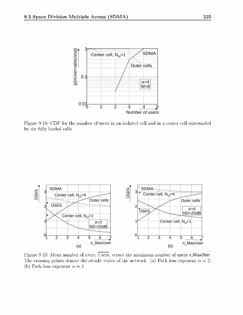
9.3 Space Division Multiple Access (SDMA) 225
Number of users0
1
1 2 3 4 50.01
0.1p(
nUse
r<ab
scis
sa)
Center cell, Ncl=1
Outer cells
M=8α=4
SDMA
Figure 9.18: CDF for the number of users in an isolated cell and in a center cell surroundedby six fully loaded cells.
n_MaxUser n_MaxUser(a) (b)
Use
rs
Use
rs
0 0
1 1
2 2
3 3
Outer cells Outer cells
Center cell, Ncl=1Center cell, Ncl=1
Center cell, Ncl=4 Center cell, Ncl=4
1 12 23 34 45 56 67 7
ND=20dB
ND=20dB
α=4
α=2
UsersUsers
SDMA SDMA
Figure 9.19: Mean number of users, Users, versus the maximum number of users n MaxUser.The crossing points denote the steady states of the network. (a) Path loss exponent � = 2,(b) Path loss exponent � = 4.

226 Capacity Enhancement
Null depth (dB)
Use
rs1.5
1
2
3
2.5
3.5
20 30 40 50
α=2
α=4
SDMA
Figure 9.20: Mean number of users, Users, versus the null depth, ND, and the front{to{backratio, FBR, of the used antenna pattern.
� = 4. Consequently, the higher the path loss, the larger the capacity increase achievable bySDMA over SFIR.
The graphs also indicate that SDMA adds exibility to the whole network. If in thesurrounding cells the tra�c is low, e.g. only one user is served per channel, the center cellcan serve two or even three users on one physical channel. This is a highly desired featureespecially for cells, where hot spots in tra�c may occur. An SDMA{component togetherwith DCA would add exibility so that a network operator can serve temporally more usersin speci�c locations without adding new BSs.
The further results examine the in uence of di�erent factors on system capacity. If notmentioned otherwise, all results are based on a cluster size of Ncl = 1, a null depth ofND=20dB, an 1D{ULA withM = 8 elements, and an CIR{threshold of CIR Threshold=15dB.
9.3.2 Null Depth and Front{to{Back Ratio
Figure 9.20 shows the mean number of users, Users, versus the null depth, ND, and thefront{to{back ratio, FBR, of the used antenna pattern. Increasing the null depth from 20dBto 40dB would increase the mean number of users by 66% for � = 2 and 83% for � = 4.
But, here it should be emphasized that real world mobile communication scenarios usuallycontain a �nite angular spread. So even an in�nite null depth would not improve systemperformance, since still some of the scatterers are illuminated by the anks of the antennapattern around the null, i.e. the nulls are �lled. The simulation model used in this chapteris build upon discrete{valued DOAs, however, by assuming a �nite null depth the e�ect ofthe angular spreading as null �lling is automatically taken into account.
As Ref. [Goo95] showed, a null depth of 20dB to 30dB seems to be reasonable for mobilecommunications. This null depth is also enough, since the increase in the mean number ofusers by utilizing antennas with ND=40dB or 50dB is only marginal compared to the valueachievable with ND=30dB.

9.3 Space Division Multiple Access (SDMA) 227
CIR_Threshold (dB)
Use
rs
1
2
3
4
9 11 13 15 17
α=2
α=4
SDMA
Figure 9.21: Mean number of users, Users, versus the CIR{threshold, CIR Threshold.
Number of antenna elements M
Use
rs
1.4
1
1.8
2.2
4 8 12 16 20 24
α=2
α=4
SDMA
Figure 9.22: Mean number of users, Users, versus the number of antenna elements, M .
9.3.3 CIR{Threshold of the System
Figure 9.21 shows the in uence of the CIR{threshold, CIR Threshold, necessary for properoperation of the system, on the mean number of users, Users. A threshold of 9dB wouldincrease the mean number of users by 120% (140%), a threshold of 12dB by 55% (57%) for� = 2 (� = 4), over the mean number of users obtained by a 15dB threshold.
Consequently, for performance assessment the parameter CIR Threshold is extremely im-portant.
9.3.4 Number of Antenna Elements
The in uence of the number of antenna elements, M , on the mean number of users is shownin Figure 9.22. The mean number of users increases strongly for M � 10, and saturates forM � 12, the saturation e�ect being stronger for smaller path loss exponents �. A systemutilizing an 1D{ULA withM = 4 can serve only 75% (82.6 %) of the users for � = 2 (� = 4)as compared to an array with M = 8, whereas an 1D{ULA with M = 12 can serve a meannumber of users which is 7% (7%) above that for M = 8.

228 Capacity Enhancement
Number of handovers, Max_Handover
Use
rs1.2
1
2
1.8
1.4
1.6
2 4 6 8 10 12 14 16
α=2
α=4 SDMA
Figure 9.23: Mean number of users, Users, versus the maximum number of handovers,Max Handover.
9.3.5 Number of Handovers
Figure 9.23 shows the in uence of the parameter Max Handover on the mean number ofusers. As the curves show, the choice of Max Handover is rather uncritical, the performanceimprovement by using 15 instead of 2 handover channels is only 13% (7%) for � = 2 (� = 4).
Therefore the considered value of Max Handover=6 for my simulations can be regarded ascharacteristic for near{optimum system performance.
9.3.6 Imperfections of the Array Processing Algorithms
Up to now I have only investigated an ideal SDMA processing chain. I will soften thiscondition here by analyzing the e�ect of pointing errors of the main beam and power controlerrors. Both errors are considered as Gaussian distributed with standard deviation �' and�PC , respectively.
Figure 9.24a shows the in uence of pointing errors of the main beam on the mean numberof users. The 3dB{beamwidth of the utilized antenna pattern is about 17�. For pointing errorswith standard deviation in the order of half of the main beam width (�' = 8�) the decreasein the mean number of users is about 19% (21%) for � = 2 (� = 4). Only for pointing errorswith standard deviation �' � 2� the capacity impairment is below 5%.
Figure 9.24b shows the in uence of power control errors on the mean number of users.Small power control errors with �PC � 2dB do not a�ect the mean number of users remark-ably. For �PC = 3dB the capacity impairment is about 6% (5%) for � = 2 (� = 4). Largerpower control errors lead to a remarkable capacity decrease, e.g. for �PC = 6dB the decreaseis 18% (16%) for � = 2 (� = 4).
9.3.7 Power Control Strategies
As in the SFIR case, I also investigated the in uence of power control strategies on the systemperformance.
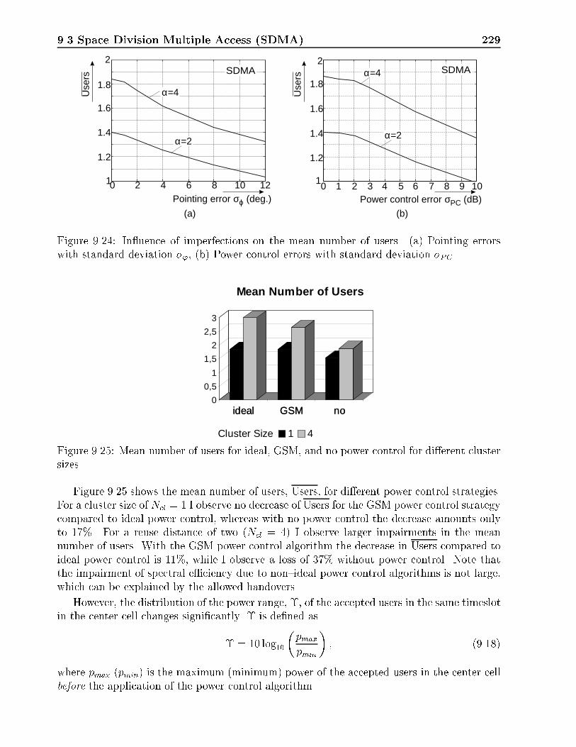
9.3 Space Division Multiple Access (SDMA) 229
Power control error σPC (dB)
Use
rs
1.2
1
2
1.8
1.4
1.6
0 1 2 3 4 5 6 7 8 9 10
α=2
α=4
Pointing error σϕ (deg.)
Use
rs
1.2
1
2
1.8
1.4
1.6
0 2 4 6 8 10 12
α=2
α=4
(a) (b)
SDMASDMA
Figure 9.24: In uence of imperfections on the mean number of users. (a) Pointing errorswith standard deviation �', (b) Power control errors with standard deviation �PC .
ideal GSM no0
0,5
1
1,5
2
2,5
3
ideal GSM no
Mean Number of Users
1 4Cluster Size
Figure 9.25: Mean number of users for ideal, GSM, and no power control for di�erent clustersizes.
Figure 9.25 shows the mean number of users, Users, for di�erent power control strategies.For a cluster size of Ncl = 1 I observe no decrease of Users for the GSM power control strategycompared to ideal power control, whereas with no power control the decrease amounts onlyto 17%. For a reuse distance of two (Ncl = 4) I observe larger impairments in the meannumber of users. With the GSM power control algorithm the decrease in Users compared toideal power control is 11%, while I observe a loss of 37% without power control. Note thatthe impairment of spectral e�ciency due to non{ideal power control algorithms is not large,which can be explained by the allowed handovers.
However, the distribution of the power range, �, of the accepted users in the same timeslotin the center cell changes signi�cantly. � is de�ned as
� = 10 log10
�pmaxpmin
�; (9.18)
where pmax (pmin) is the maximum (minimum) power of the accepted users in the center cellbefore the application of the power control algorithm.

230 Capacity Enhancement
0 10 20 30 400
10
20
30
40
50
606
Samples
-�
� = 24:5dB�� = 34:1dBP1User=20.5%
(a)
0 10 20 30 400
10
20
30
40
50
60
70
806
Samples
-�
� = 26:2dB�� = 36:5dBP1User=0.5%
(d)
0 10 20 30 400
10
20
30
40
50
60
70
806
Samples
-�
� = 16:8dB�� = 21:4dBP1User=21.3%
(b)
0 10 20 30 400
10
20
30
40
50
60
70
806
Samples
-�
� = 18:3dB�� = 22:8dBP1User=5.1%
(e)
0 10 20 30 400
50
100
150
2006
Samples
-�
� = 2:1dB�� = �3:1dBP1User=48.2%
(c)
0 10 20 30 400
50
100
150
200
2506
Samples
-�
� = 2:5dB�� = �2:6dBP1User=23.6%
(f)
No Power Control
GSM Power Control
Ideal Power Control SDMA
Figure 9.26: Distribution of �. (a) { (c) for cluster size Ncl = 1, (d) { (f) for cluster sizeNcl = 4 with ideal, GSM, and without power control, respectively.

9.4 Conclusions 231
Omnidirectional antennas Sector antennas
� = 2 � = 4 � = 2 � = 4Sector antenna 3.1 2.3 1 1
Ncl = 3 16.3 2.3 5.3 1SFIR
Ncl = 1 49 7 16 3
Ncl = 3 36.7 6.4 11.9 2.8SDMA
Ncl = 1 68.6 12.6 22.4 5.4
Table 9.1: Increase in spectral e�ciency for the tra�c channels by the application of smartantennas as compared to systems using omnidirectional or sector antennas.
Figure 9.26 shows the distribution of the power range, �, of the accepted users in thecenter cell. A small value of � means that only users with similar power levels can be servedsimultaneously in one cell. The cases, where only one user is accepted, which means that� = 0dB, are not included in the distribution. Instead, the percentage that only one user isaccepted in the center cell, P1User, is indicated.
Figures 9.26c and f show that, without any power control, � is 5dB at maximum. Thiscomes from the fact that the maximum suppression of co-channel interferers is ND = FBR =20dB, while a CIR{value of CIR Threshold = 15dB is required for a user to be accepted. Thedi�erence of these values gives the maximally allowed ratio of the powers of two acceptedusers. As a consequence the users have to be grouped into so{called power classes [Tan95]with a range of 5dB each, i.e. for a realistic dynamic range of a cell of about 80dB, 16(!)tra�c channels for handovers would be necessary. Otherwise, not the whole cell area couldbe served simultaneously.
For the employment of the GSM or the ideal power control algorithm the spread of �is much larger (standard deviation of �, �� > 21dB) than in the case of no power control(�� � �3dB). Here, the requirements for the grouping of users into power classes are lessstringent. Although I did not observe a reduction of the mean number of users for the caseof GSM power control compared to ideal power control, the distribution of � has changed.For the GSM scenario smaller values of � became more probable (the mean value of �, �, isabout 8dB smaller than in the case of ideal power control) and situations where � > 30dBnearly vanish. The �rst statement can be explained due to the inherent power control error ofthe GSM scenario (maximum error of �1dB and lognormal fading), and the second statementcomes from the limited dynamic range of the GSM power control of 30dB.
9.4 Conclusions
This chapter investigated the spectral e�ciency increase achievable by using smart antennas.Table 9.1 shows the increase in spectral e�ciency for both SFIR and SDMA as compared tosystems using omnidirectional or sector antennas.
A cluster size of Ncl = 1 for the tra�c channels is possible by using SFIR. The used1D{ULA should have a number of elements M � 8, a null depth and front{to{back ratio of

232 Capacity Enhancement
at least 20dB, and should cover a sector of 90� or 120�. This means that three or four smartantennas replace one conventional omnidirectional antenna.
My estimates for the capacity increase are comparable to those of Refs. [Tan94] and[Lop96]. Note that the di�erent values are primarily caused by the fact that these tworeferences use circular arrays. If one wants to make a comparison between my and theirresults, the number of circular antenna elements has to be replaced by three times the numberof antenna elements used in my simulations. Additionally I am allowing for handovers, whichactually is a variant of DCA, and I do not assume the interference to be uniformly distributed.My estimates are of course only valid if the angular spread of the scenario is below half of the3dB beamwidth of the BS antenna, which is about 8:5�. Consequently most of the cases arecovered (see also Chapter 2, Figure 2.11). Furthermore, I have assumed that the dynamicrange of the power control is large enough to cover the whole dynamic range of the mobileradio channel. Should this not be the case, the cell has to be divided into several concentricrings, where each one forms a so{called power class [Tan95]. This would of course decreasethe spectral e�ciency of the system, but Ref. [Tan95] showed this decrease to be only modest.
My estimates seem also to be restricted to situations where the signal of the wanted usercomes primarily from one nominal direction associated with an angular spread. However,this is a viable assumption for typical SDMA{scenarios [Kle96b], [Bul95].
The results for SFIR show that the standard deviation, �', of the directional estimateof the nominal DOA has to be less than 3� for a 1D{ULA with M = 8 elements and thestandard deviation of the power control error has to be less than 3dB as not to decreasesystem performance.
SDMA provides a capacity increase of 40% (126%) for a path loss exponent of � = 2 (� =4) over SFIR. This increase seems to be rather modest as compared to the increase achievableby SFIR alone. SDMA, however, provides the system with more exibility, since temporallyoccurring hot spots in speci�c locations can be dealt with without making hardware changesto the whole network. The SDMA{component needs only to be introduced in such cellswhere one needs more capacity, whereas SFIR has to be implemented in the whole system toachieve the full capacity increase.
The choice of the antenna (number of elementsM , ND, SLL, FBR) and the CIR{thresholdof the system are the parameters to which a performance assessment is most sensitive, whereasthe number of handover channels is rather uncritical.
I have also assumed that the power control reacts without delay. This is not true in areal GSM system, where power equalization is delayed. To account for that e�ect, powercontrol errors can be considered. My results indicate that an SFIR system can cope withlarger power control errors than an SDMA system.
The non{ideal power control strategies give only slightly lower estimates for the spectrale�ciency. For the case of SFIR, the spectral e�ciency even stays the same. However, Iobserved an increased number of handovers, which reduces the overall capacity of a networkdue to an increased signaling load. Additionally, in con�gurations with larger cluster sizes Iobserved a reduced quality of the system, i.e. smaller values for CIR5%.
In the case of SDMA, the spectral e�ciency degraded signi�cantly only for systems with nopower control. Note, however, that the quality of the power control strategy has signi�cantin uence on the channel allocation and handover schemes, since a large number of powerclasses has to be introduced. This would of course decrease the spectral e�ciency of the
9.4 Conclusions 233
system.
Sophisticated power control strategies are, especially for SDMA systems, necessary tokeep the system complexity low, and to fully exploit the increase in system performance bysmart antennas.
In conclusion, SDMA provides only marginal capacity increase as compared to a pureSFIR system, but it provides more exibility to the network and enables partial systemupgrading to account e.g. for hot spots, whereas SFIR has to be employed in rather largeareas to give the wanted capacity increase.


Chapter 10
Some Protocol Aspects of SmartAntennas
There are two di�erent ways to employ smart antennas at the BS, depending on the generationof the mobile communications system.
� In a second generation system (like GSM, IS{54, IS{136, etc.) it should be possible toadd a smart antenna without any change in the system speci�cations. This means thatone has to �nd a concept for smart antennas within the framework of the standard.
� For the standardization of a third generation system the requirements of smart antennashave to be considered to fully exploit their potential.
This chapter deals with some of these questions. It highlights some of the missing protocolparts in second generation systems on the example of GSM and comments on the protocolrequirements for a third generation system.
The impacts of SDMA on a 2nd generation system are twofold:
� on the hard- and software of the BS, and
� on the protocols.
While I have been dealing with the �rst issue already in Chapter 2, I will here concentrateon the second one. I will examine four di�erent problems:
� call setup,
� power control
� the BCCH (Broadcast Control CHannel){problem, using the GSM as example for a2nd generation system, and
� handovers.
Some of these issues have also been dealt with in the References [Tan95] and [Cla96].
235

236 Some Protocol Aspects of Smart Antennas
10.1 Call Setup
We have to distinguish two di�erent call setup procedures in GSM:
1. MOC (Mobile Originated Call)
2. MTC (Mobile Terminated Call)
The basic procedures are described e.g. in [Mou92] and [Cme20]. Therefore I will here onlyfocus on the starting point of a call.
� MOC (Mobile Originated Call)
The MS uses RACH (Random Access CHannel) to request a signaling channel, SD-CCH (Stand{alone Dedicated Control CHannel) for setting up the call. Since theBS does not know where the MS is located and no training sequence is inserted inthe RACH{burst, only algorithms needing no training sequence (e.g. CMA, switchedbeam, and SR algorithms) can be used to exploit the available directional antenna gain.
� MTC (Mobile Terminated Call)
The BTSs in the wanted location area of the mobile transmit the paging message overthe air interface using the PCH (Paging CHannel). Since no information about thelocation of the mobile is available, the message has to be transmitted in an omnidirec-tional mode of the BS antenna. To achieve the same receive power level at the MS as inthe case using a smart antenna, the transmit power of the BTS has to be increased by avalue proportional to the antenna gain. Note that omnidirectional transmission meansthat this channel has to be placed in a reuse pattern like the one in a system usingomnidirectional antennas. This of course means that the capacity increase is reduced.
After successful call setup, a TCH (Tra�c CHannel) is allocated for the call. SFIR systemsserve only one user (call) per tra�c channel. However, as I have shown in Chapter 9, thereare some situations, where the CIR on that channel is below the necessary threshold forsuccessful communication | especially for densely reused frequencies. Here, I regard DCA,which is equivalent to allow for handovers, of great help in making the best use of the availablespectrum.
For the SDMA operation mode of the system we have to know some additional propertiesof the propagation channel, which are
� the DOAs and
� the power of the incident signals, from which the power class of the mobile can bedetermined [Tan95].
This information is not used in today's systems. The following paragraph gives my viewabout one possible workaround:

10.2 Power Control 237
It has to be transmitted over the Abis{interface to the BSC, where it forms an input forthe channel allocation scheme. I regard this as possible even in today's GSM systems,since messages across this interface are partly proprietary, so that messages can, inprincipal, be added. Since we have to know the spatial properties of the propagationchannel before making a TCH assignment at the BSC, the information derived fromthe reception of the RACH and the SDCCH can be used to extract this information,or, the call is started in a channel with a potentially high CIR, i.e. a channel, whereonly the desired user is present. After an exact determination of the properties of thepropagation channel the call is transferred to the speci�c TCH. One possibility is to �llup every TCH with just one call (SFIR) until the system is fully loaded. Only slightlybefore the full{load situation occurs, the SDMA{mode of the system is invoked.
10.2 Power Control
Although not a protocol issue, I will treat power control in this context due to its signi�cancefor an SDMA system.
If the dynamic range of the power control is too small to cover the whole range of achannel, which might be 60{100dB, the mobiles can be grouped into power classes [Tan95].In space, the power classes are | in ideal simpli�cation | concentric rings around the BS.Reference [Tan95] showed that the ratio of the boundaries of one power class in space is givenby
rc+1rc
= 10PL=(10�); (10.1)
where rc and rc+1 are the radii of the boundaries belonging to one power class and PL is themaximum path loss permitted in one power class. Obviously, the size of the power classesfor a certain PL depends only on the pathloss exponent �. The power classes should be aslarge as possible to keep the loss of trunking gain within limits. Ref. [Tan95] showed thatthe decrease in trunking gain is about 20% for PL = 20dB and � = 4, which is not much.
On the other hand, the size of a power class, PL, is dependent on the link budget. Itshould be small enough to guarantee su�cient receive SNR at the MS.
I will now examine a typical case. Assume that two users are received at the BS. The�rst has a signal level of P1 = �70dBm, whereas the second has P2 = �90dBm. Assumingan antenna with ND=30dB, we would get for the CIRs at the BS, BS� CIR1 = 50dBand BS� CIR2 = 10dB, assuming ideally placed nulls. Both CIRs would be su�cient forsuccessfully processing of the users' signals. If we now want to balance the users in terms ofSNR at the MSs, although we do not know the noise oor at the mobile, we would increasethe transmission power for User 2 by 20dB over that for User 1 (P2 = P1 + 20dB). However,since the nulldepth is 30dB, we would get for the CIRs at the mobiles MS1 � CIR = 10dBand MS2 � CIR2 = 50dB, which is just the inverse situation of the uplink.
Usually, the power control of the mobile is adjusted in a way as to give the same meanpower to all wanted signals at the BS. But, the situation is even further complicated, if thedynamic range of the power control is higher than the nulldepth of the antenna. Then, ofcourse, the signals can have the same mean power at the uplink. E.g. assume that User 1su�ers a propagation loss that is 40dB below that of User 2. If the MS power control can

238 Some Protocol Aspects of Smart Antennas
CIR-Uplink CIR-Downlinkwith signal
powerbalancing
CIR-Downlinkwith
interferencebalancing
05
101520253035404550
CIR
(d
B)
CIR-Uplink CIR-Downlinkwith signal
powerbalancing
CIR-Downlinkwith
interferencebalancing
Uplink and Downlink CIRs
User 1
User 2
Figure 10.1: CIR{values for the uplink and downlink by application of di�erent power controlstrategies (signal power balancing and interference balancing) at the downlink.
compensate for this e�ect (I assume, that its dynamic range is above that used in today'sGSM system, which is 30dB maximum), the signals of the two users are received with thesame power at the BS. However, full compensation of the di�erent propagation losses at thedownlink is impossible, since the di�erence (40dB) is larger than the nulldepth (ND=30dB)of the used antenna.
One way out of this problem is to realize that mobile communications systems are usuallyinterference limited. So we do not have to compensate for the additional propagation loss,since not the SNR is the limiting parameter, but the CIR. Consequently only the CIR hasto be balanced at the downlink. Therefore no power control is applied at the downlink,so that both users now have a CIR of MS1(MS2)� CIR = 30dB. Of course, the SNRs aredi�erent, SNR2 = SNR1 � 30dB (if the noise levels at the mobiles are the same), but, asmentioned above, this causes no problems to interference limited systems. Figure 10.1 showsa comparison of the CIR values at the uplink and the CIR values for the two approaches(signal power balancing and interference balancing) at the downlink.
In general, in SDMA systems no power control should be applied at the downlink in orderto maintain equal CIRs for all users served on the same tra�c channel | interferencebalancing.
Again, this argument indicates that system performance is determined by the downlink.One method to improve downlink performance is to increase the transmit power for thedownlink. But this also increases the interference to neighboring cells. This leads to theproblem that in an SDMA mode both the wanted signal and the dominating interferingsignal for a speci�c user are subject to the same large{scale fading, since they propagatealong the same paths. Figure 10.2 shows a possible scenario. Two users are served in thesame tra�c channel. The corresponding radiation patterns and the propagation paths areshown. I used this scenario to investigate whether the small{scale fading of wanted signaland of interference is also correlated. The radius of the scatterer circle was set to R = 200�,

10.2 Power Control 239
User 1Desired signal
Desired signal
Interference
Interference
BS
User 2
2R
Figure 10.2: Scenario showing the propagation paths of desired signals and interference fortwo users in an SDMA system.
the number of scatterers was set to Ns = 80, the distance between the MS and the BS, rMS,was varied from rMS = 200� to rMS = 20000�. Four di�erent situations are considered:
� Beamforming by using the pseudoinverse.
� Beamforming, whereby the nulls are �lled to 30dB below the maximum.
� Beamforming with broad nulls. The �rst order derivative is set to zero.
� Hole burning. The 20 scatterers nearest to the MS (in azimuthal angle ' as seen fromthe BS) were eliminated for calculation of the interference.
The CIR at the MS was calculated and its correlation coe�cient, �CIR, determined. Therange of the results is given in Figure 10.3. Since the correlation coe�cients were found tobe always less than 10�2, the small{scale fading is uncorrelated. This somewhat surprisingresult is due to the di�erent antenna patterns for the wanted signal and the interference, i.e.the signals propagating di�erent ways have also been weighted di�erent (by their associatedantenna pattern) at the BS.
Having shown that
� large{scale fading of wanted and interfering signal is correlated, but
� small{scale fading is not,
I can draw two interesting conclusions.
First, in the link budget we have to include only a fading margin for the small{scalefading. Second, since the small{scale fading is uncorrelated, antenna diversity at the mobilewould still be e�ective in increasing the CIR.

240 Some Protocol Aspects of Smart Antennas
0 5 10 15 20 2510
−16
10−14
10−12
10−10
10−8
10−6
10−4
10−2
100
6
�CIR
-rMS (1000�)
Figure 10.3: Interval of the correlation coe�cient �CIR of the CIR variation due to small scalefading.
10.3 The BCCH{Problem
This section follows the lines of argument of Ref. [Cla96]. The primary requirement of com-mon downlink channels is to achieve complete coverage of the wanted cell and some overlapto surrounding cells. In GSM/DCS 1800 the beacon carrier (BCCH) must be broadcast atall times at constant power. This enables the MSs from neighboring cells to continuouslyperform measurements on that frequency. In consequence, these channels must be sent in anomnidirectional mode of the antenna. This would, however, completely disturb our small co{channel reuse ratio system, since we de�nitely cannot use the same frequency for the BCCHat each BTS as for the tra�c channels. The solution to this problem is to transmit the BCCHon di�erent frequencies in adjacent cells, i.e. to utilize a reuse pattern as in a conventionalsystem. For that reason, the system has to have two di�erent co{channel reuse distances, one( ~Q) for the tra�c channels, and a second one ( ~QBCCH) for the BCCH{carrier and the PCHfrequency. Therefore, again, careful cell planning has to be done for the BCCH{frequencies.
10.4 Handovers
Processing handovers is an important task in any cellular communication system. The entiresystem quality depends on the way how proper handover margins are determined and howthey are applied to the given cell structure. Usually handovers are prioritized over callinitiation requests. From a user's point of view, having a call abruptly terminated in themiddle of a conversation is much more annoying than being temporally blocked on a newcall attempt [Rap96]. I regard a handover of a user served in a directional mode of the BSantenna as much more critical than in a conventional system, for three reasons,
1. the new BTS does not know the angular position of the mobile,

10.4 Handovers 241
2. the new BTS does not know the user's angular spread, and
3. it does not know the power class of the mobile.
Case (1) can be worked around if the handover takes place between two BTS's connected tothe same BSC (they could exchange data over the Abis{interface). However, for handoversbetween BTSs belonging to di�erent BSCs the DOA has to be determined anew at the newtra�c channel, since the protocols for the message ow at the GSM A{interface is speci�edmuch more strictly.
The "old" BTS knows the DOAs and the timing advance of the mobile. Therefore its po-sition can be determined up to �500m (step size of the timing advance). This uncertainty issurely too large to support beam{to{beam handover procedures as proposed in Ref. [Tan95].Another approach is to use propagation time di�erences to di�erent BTS to determine thelocation via some kind of trilateration. The �eld trial of Ref. [Bun95] showed that a meanerror of 300m is achievable with such an approach. But, in GSM we have only the tim-ing advance to one BTS, therefore handovers have to be enforced. This approach has thedisadvantage of generating a high signaling load onto the system. A further idea is to useGPS (Global Positioning System) in conjunction with GSM to get the location data. For ahandover this data is of course only useful, if the majority of the power really comes fromthe surrounding of the mobile. This assumption is, in fact, valid for most of the scenarioswhere SFIR and/or SDMA is an issue to deal with [Kle96b]. And, since we now know boththe coordinates of the BS and the MS and the DOAs of the incident signals, we can checkwhether this assumption is ful�lled.
The available information would be passed together with the value of the received powerover the Abis{interface (running a modi�ed protocol) to the BSC for channel allocation, or,channel allocation would be done directly at the BTS. All this information could also bepassed to the new BTS, if it is within the control of the same BSC. However, the BTS couldonly partially make use of this information, since the (new) received power and the (new)angular spread of the signals are unknown. They could only be reliably determined after aninitial transmission of the MS to the new BTS. The tra�c channel of the new BTS, where thehandover should be performed to, has to be a "free" physical channel of the new BTS. Afterthe user characteristic has been determined at the new BTS, the call can be handovered toa di�erent tra�c channel, if necessary. To make at least partial use of the available antennagain at the new BTS for the handover, a blind algorithm, a switched beam approach, or anSR approach could be utilized [Rhe95].
Another, conceptually di�erent handover situation occurs, if any two users at the sameTCH are too near in angle, so that they could no be separated successfully anymore byspatial processing. The angle threshold 'th basically depends on the angular spread of theenvironment and the beamwidth of the BS antenna. For this situation a handover to adi�erent TCH within the same BTS has to be performed. Since the BTS knows the DOAs,the angular spread, and the power class of the mobile, the handover can be done onto a TCHalready operating in an SDMA{mode, since the characteristics would stay about the same,if we only change the frequency within the allocated band. Nevertheless this procedure isquite challenging for a conventional BTS.
To ensure successful handovers between BTSs, a number of channels can be reserved forhandover purposes only, which is called the guard channel concept [Rap96]. This approachfaces the disadvantage of being a capacity{killer.

242 Some Protocol Aspects of Smart Antennas
10.5 Others
The downlink poses some problems to the system, especially if FDD is used to separate itfrom the uplink. Therefore TDD, leading to a high correlation of the fading in the up{ andthe downlink, would simplify some of the problems related to smart antennas.
Constraints due to today's systems are further imposed by the training sequences (length,correlation properties). One BTS uses only one dedicated training sequence out of the 8speci�ed sequences ("color code") for GSM. The remaining sequences are used by othersurrounding BTSs using the same frequency slot, to distinguish co{channel interferers. Fora system operating in an SDMA{mode, more than one sequence has to be used at one BS.
The impacts of an SDMA component on a 3rd generation systems depends on the trans-mission format to be chosen and other features of the system. It also depends on the typeof algorithmic approach chosen for the SDMA{step (blind algorithm, non{blind algorithm).This will a�ect the training sequences, if there will be any, in terms of length, correlationproperties, and type of sequence. Also, handover algorithms need to be changed, traditionalchannel allocation schemes and frequency planning (cell planning) have to take into accountthe SDMA{component. DCA is an especially attractive feature to work with SDMA (seealso Chapter 9). Also a closer look on power control issues has to be taken.
However, there are no real restrictive requirements of an SDMA{component on the trans-mission format of a future system. These systems should be "SDMA{friendly", facilitatingtheir use, but not specifying any way on how to implement them [Bul95].

Bibliography
[Abr65] M. Abramowitz, I. A. Stegun. Handbook of Mathematical Functions, Dover Publica-tions, Inc., New York, 1965.
[Ada86] F. Adachi, M. T. Feeney, A. G. Williamson, J. D. Parsons. "Crosscorrelation betweenthe envelopes of 900 MHz signals received at a mobile radio base station site", IEEProceedings, Vol. 133, Pt. F, No. 6, October 1986, pp. 506{512.
[Ada89] F. Adachi, J. D. Parsons. "Error Rate Performance of Digital FM Mobile Radiowith Postdetection Diversity", IEEE Trans. on Communications, vol. 37, no. 3, March1989, pp. 200{210.
[Aka74] H. Akaike. "A New Look at the Statistical Model Identi�cation." IEEE Trans. onAutomatic Control, vol. AC{19, no. 6, December 1974, pp. 716{723.
[Ale84] S. T. Aleksander. "A Derivation of the Complex Fast Kalman Algorithm", IEEETrans. Acoustics, Speech, and Signal Proc., vol. ASSP{32, no. 6, December 1984, pp.1230{1232.
[Ali93] M. E. Ali, J. G�otze, and R. Pauli. "An Algorithm for the Calibration of Sensor Arrayswith Sensor Gain and Phase Uncertainties." Proc. IEEE Int. Conf. Acoust., Speech,Signal Processing, Volume IV, pp. 121{124, Minneapolis, MN, April 1993.
[Ali94] M. E. Ali{Hackl, M. Haardt, and J. A. Nossek. "4xS{Single Snapshot Spatial Sepa-ration of Wavefronts via Antenna Arrays." Proc. 8. Aachener Kolloquium Signaltheorie,Aachen, March 1994, pp. 369{372.
[And91] S. Anderson, M. Millnert, M. Viberg, B. Wahlberg. "An Adaptive Array for MobileCommunication Systems," IEEE Trans. on Vehicular Technology, vol. 40, no. 1, February1991, pp. 230{236.
[ArC96] Open Channels, News and Notes on ArrayComm Activities, Vol. 1, Iss. 1, Fall 1996.
[Bac89] J. Bach Andersen. "A Note on De�nitions of Terms for Impulse Responses", COST231 TD(89)60, October 18, 1989.
[Bac86] J. Bach Andersen, S. L. Lauritzen, C. Thommesen. "Statistics of Phase Derivates inMobile Communications", Proc. 36th IEEE Vehicular Technology Conference, Dallas,USA, May 1986, pp. 228-231.
[Bar86] H. J. Bartsch. Mathematische Formeln, VEB Fachbuchverlag Leipzig, 1986.
243
244 Bibliography
[Bau92] D. Bauer. "Einheitliche Beschreibung ged�achtnisbehafteter sequentieller Detek-tionsverfahren f�ur gest�orte interferenzbehaftete Daten�ubertragungssysteme", AE�U, vol.46, 1992, no. 1, pp. 39{53.
[Bel63] P. A. Bello. "Characterization of Randomly Time Varying Linear Channels", IEEETrans. on Communications, Volume CS{11, December 1963, pp. 360{393.
[Bie77] G. J. Biermann. Factorization Methods for Discrete Sequential Estimation, AcademicPress, New York, 1977.
[Big95] L. Bigler, H. P. Lin, S. S. Jeng, G. Xu. "Experimental Direction of Arrival andSpatial Signature Measurements at 900 MHz for Smart Antenna Systems", Proc. 1995IEEE 45th Vehicular Technology Conference, Chicago, Illinois, USA, July 25{28, 1995,pp. 55{58.
[Bla95] J. J. Blanz, P. W. Baier and P. Jung. "A Flexibly Con�gurable Statistical ChannelModel for Mobile Radio Systems with Directional Diversity". Proc. 2. ITG{FachtagungMobile Kommunikation '95, Neu{Ulm, September, 26{28, 1995, pp. 93{100.
[Bla96] J. J. Blanz, A. Klein, W. Mohr. "Measurement{based parameter adaptation of wide-band spatial mobile radio channel models." Proc. IEEE ISSSTA '96, Mainz, Germany,pp. 91{97.
[Bot95] G. E. Bottomley, K. Jamal. "Adaptive Arrays and MLSE Equalization", Proc. 46thVehicular Technology Conference, VTC'96, Atlanta, GA, USA, April 28{May 1, 1996,pp. 50{54.
[Bre86] Y. Bresler, A. Macovski. "On the Number of Signals Resolvable by a Uniform LinearArray." IEEE Trans. Acoust., Speech, Signal Processing, vol. ASSP{34, pp. 1361{1375,December 1986.
[Bue94] H. B�uhler. "Estimation of Radio Channel Time Dispersion for Mobile Radio NetworkPlanning", Doctoral Dissertation, INTHF, TU Wien, Vienna, Austria, October 1994.
[Bul95] T. Bull, M. Barrett, R. Arnott. "Technology in Smart Antennas for UNiversal Ad-vanced Mobile Infrastructure (TSUNAMI R2108) | Overview". Proc. RACE MobileTelecommunications Summit, Cascais, Portugal, November 22{24, 1995, pp. 88{97.
[Bun95] U. B�uning, S. Gl�uckmann, "Untersuchung von Ortungsm�oglichkeiten im GSM{Netz", Ortung und Navigation, 1:21{31, 1995.
[Bur81] G. J. Burke, and A. J. Poggio. "Numerical Electromagnetics Code (NEC) | Methodof moments," Parts 1,2, and 3. Lawrence Livermore Laboratory, 1981.
[Cal96] M. H. Callendar, "IMT{2000 (FPLMTS) Standardization", Proc. ACTS MobileTelecommunications Summit, Granada, Spain, November 27{29, 1996, pp. 27.
[Car83] G. Carayannis, D. G. Manolakis, N. Kalouptsidis. "A Fast Sequential Algorithm forLeast{Squares Filtering and Prediction", IEEE Trans. Acoustics, Speech, and SignalProc., vol. ASSP{31, no. 6, December 1983, pp. 1394{1402.

245
[Che92] S. Chen, B. Mulgrew. "Overcoming Co{Channel Interference Using an AdaptiveRadial Basis Function Equaliser", Signal Processing 28 (1992), pp. 91{107.
[Cic94] D. J. Cichon, Strahlenoptische Modellierung der Wellenausbreitung in urbanen Mikro-und Pikofunkzellen, Doctoral Dissertation, Karlsruhe, Germany, 1994.
[Cio84] J. M. Cio�, T. Kailath. "Fast, Recursive{Least{Squares Transversal Filters forAdaptive Filtering", IEEE Trans. Acoustics, Speech, and Signal Proc., vol. ASSP{32,no. 2, April 1984, pp. 304{337.
[Cla96] J. W. Clarkson, "An Advanced Antenna System | Unplugged", Proc. ACTS MobileTelecommunications Summit, Granada, Spain, November 27{29, 1996, pp. 302{307.
[Col87] R. E. Collin. Antennas and Radiowave Propagation, Mc{Graw Hill Book CompanyInc., 1985.
[Cme20] CME 20 System Survey, Training Document, Ericsson Radio Systems AB, 1994,Stockholm, Sweden.
[Cor94] I. R. Corden, M. Barrett. "Adaptive Antennas for Second and Third GenerationMobile Systems," RACE Mobile Telecommunications Workshop, May 17{19, 1994, Am-sterdam, pp. 728{732.
[Cos89] Commission of the European Communities. Digital land mobile radio communica-tions | COST207, ECSC{EEC{EAEC, Luxembourg, 1989.
[Cro91] I. Crohn. "Short{Term Modelling of the Land Mobile Radio Channel", DoctoralDissertation, INTHF, TU Wien, Vienna, Austria, May 1991.
[DAr91] G. D'Aria, R. Piermarini, V. Zingarelli. "Fast Adaptive Equalizers for Narrow{BandTDMA Mobile Radio", IEEE Trans. on Vehicular Technology, vol. 40, no. 2, May 1991,pp. 392{403.
[Dew92] J. P. de Weck, "Real{Time Characterization of Wideband Mobile Radio Channels",Doctoral Dissertation, INTHF, TU Wien, Vienna, Austria, June 1992.
[Doi96] Y. Doi, T. Ohgahne, E. Ogawa, "ISI and CCI Canceller Combining the AdaptiveArray Antennas and the Viterbi Equalizer in a Digital Mobile Radio." Proc. IEEE 46thVehicular Technology Conference, VTC '96, Atlanta, Georgia, USA, April 28 { May 1,1996, pp. 81{85.
[DuH73] Duda & Hart. Pattern Classi�cation and Scene Analysis, John Wiley and Sons,1973.
[Egg94] P. C. F. Eggers, "TSUNAMI: Spatial Radio Spreading as Seen by Directive Anten-nas", European cooperation in the �eld of scienti�c and technical research, COST 231TD(94)119, Darmstadt, Germany, September 6{8, 1994.
[Egg95a] P. C. F. Eggers. "Angular Dispersive Mobile Radio Environments sensed by highlyDirective Base Station Antennas." Proc. 6th Personal, Indoor and Mobile Radio Con-ference 1995, PIMRC '95, Toronto, Canada, pp. 522{526.

246 Bibliography
[Egg95b] P. C. F. Eggers, "Quantitative Descriptions of Radio Environment Spreading Rel-evant to Adaptive Antenna Arrays", Proc. 1st European Personal and Mobile Commu-nications Conference, EPMCC'95, Bologna, Italy, November 28{30, 1995, pp. 68{73.
[Egg96] P. C. F. Eggers. "Directional Propagation Characterization",R2108/AUC/WP1.2/DN/P/054/a1, Alborg University Center, January, 18, 1996.
[Erb96] H. Erben, J. S. Dasilva, B. Barani, D. Ikonomou, "European R&D Towards Thirdgeneration Mobile Communications Systems", International Conference on Telecommu-nications 1996, ICT'96, April 14{17, 1996, Istanbul, Turkey, pp. 661{666.
[Eva81] J. E. Evans, J. R. Johnson, and D. F. Sun. "High Resolution Angular SpectrumEstimation Techniques for Terrain Scattering Analysis and Angle of Arrival Estimation,"Proc. 1st ASSP Workshop Spectral Estimation, Hamilton, Ont., Canada, 1981, pp. 134{139.
[Far95a] C. Farsakh, J. Nossek. "Channel Allocation and Downlink Beamforming in anSDMA Mobile Radio System", Proc. 6th Personal, Indoor and Mobile Radio Confer-ence 1995, PIMRC '95, Toronto, Canada, pp. 687{691.
[Far95b] C. Farsakh, M. Haardt, J. A. Nossek, and K. Pensel. "Adaptive Arrays in MobileRadio Systems", Proc. 2nd ITG Fachtagung Mobile Kommunikation '95, Ulm, Germany,September 26{28, 1995, pp. 101{108.
[Far96a] C. Farsakh. "Simulation eines SDMA{Systems", Seminar Presentation, TU Wien,Vienna, April 1996.
[Far96b] C. Farsakh, J. Nossek, "On the Spatial Separation Potential of a Uniform LinearArray", Proc. 46th Vehicular Technology Conference, VTC'96, Atlanta, GA, USA, April28{May 1, 1996, pp. 1477{1480.
[Far96c] C. Farsakh, J. A. Nossek, "A Real{Time Downlink Channel Allocation Scheme foran SDMAMobile Radio System", Proc. 7th IEEE International Symposium on Personal,Indoor and Mobile Radio Communications, PIMRC '96, October 15{18, 1996, Taipeh,Taiwan, ROC, pp. 1216{1220.
[Fes94] J. A. Fessler, A. O. Hero, "Space{Alternating Generalized Expectation{MaximizationAlgorithm", IEEE Trans. on Signal Processing, vol. 42, October 1994, pp. 2664{2677.
[Fil93] V. Filimon, W. Kozek, W. Kreuzer, G. Kubin. "LMS and RLS Tracking Analysis forWSSUS Channels", Proc. IEEE ICASSP '93, Minneapolis, MN, pp. III{348 { III{351,April 1993.
[Fle90] B. Fleury, Charakterisierung von Mobil{ und Richtfunkkan�alen mit schwach sta-tion�aren Fluktuationen und unkorrelierter Streuung (WSSUS), Dissertation, ETHZ�urich, 1990.
[For72] G. D. Forney, Jr. "Maximum{Likelihood Sequence Estimation of Digital Sequencesin the Presence of Intersymbol Interference", IEEE Trans. on Information Theory, vol.IT{18, no. 3, May 1972.

247
[Fuh95a] J. Fuhl, A. F. Molisch, "Virtual Image Array Single Snapshot (VIASS) Algorithmfor Direction{Of{Arrival Estimation of Coherent Signals." Proc. 5th Personal, Indoor,and Mobile Communications Conference 1995, Toronto, 1995, pp. 658{663.
[Fuh95b] J. Fuhl, A. F. Molisch, "Space Domain Equalization for Second and Third Gener-ation Mobile Radio Systems", Proc. 2. ITG{Fachtagung Mobile Kommunikation, Neu{Ulm, September 1995, 26{28, pp. 85{92.
[Fuh95c] J. Fuhl, E. Bonek, P. Balducci, P. Nowak, and H. Garn. "Internal Antenna Ar-rangements for Personal Communication Systems", Proc. 1st EPMCC '95, Bologna,Italy, 28{30 November 1995, pp. 62{67.
[Fuh96b] J. Fuhl, E. Bonek. "Space{Time Decomposition: Exploiting the Full Informationof a Training Sequence for an Adaptive Array", Electronics Letters, 10th October 1996,Vol. 32, No. 21, pp. 1938{1940.
[Fuh97] J. Fuhl, J. P. Rossi, E. Bonek, "High{Resolution 3D Direction{Of{Arrival Determi-nation for Urban Mobile Radio", To appear in IEEE Trans. on Antennas and Propaga-tion, April 1997.
[Gar95] Q. Garcia, F. Municio, "Broadband Basestation Arrays and Antenna Elements forMobile Communications", Proc. 1st European Personal and Mobile CommunicationsConference, EPMCC'95, Bologna, Italy, November 28{30, 1995, pp. 56{61.
[Ger93] D. Gerlach, A. Paulraj, "Base Station Transmitter Antenna Arrays with Mobile toBase Feedback", Proc. 27th Asilomar Conference on Signals, Systems and Computers,vol. 2, 1993, pp. 1432{1436.
[Ger94] D. Gerlach, A. Paulraj, "Adaptive Transmitting Antenna Methods for MultipathEnvironments", GLOBECOM '94, San Francisco, CA, USA, 1994, pp. 425{429.
[Ger96] A. B. Gershman, G. V. Serebryakov, J. F. B�ohme, "Constrained Hung{Turner Adap-tive Beamforming Algorithm with Additional Robustness to Wideband and MovingJammers", IEEE Trans. on Antennas and Propagation, vol. 44, no. 3, March 1996, pp.361{367.
[Gia96] D. Giancristofaro, "Correlation Model for Shadow Fading in Mobile Radio Chan-nels", Electronics Letters, 23rd May 1996, vol. 32, no. 11, pp. 958{959.
[Gol94] M. Goldburg, R. H. Roy. "The Impacts of SDMA on PCS System Design", Proc.3rd Annual International Conference on Universal Personal Communications, 1994, pp.242{246.
[Gol83] G. H. Golub, C. F. van Loan.Matrix Computations. Johns Hopkins University Press,Baltimore, Maryland, 1983.
[Goo95] M. J. Goonan, W. F. Hancock, J. Kalisz, J. D. Kisby, S. J. Lloyd, L. McCallum, D.J. McMillan, W. L. Reiners, "Developement of Multiple Beam Antennas for TerrestrialApplications", 1995 Workshop of Radio Science (WARS '95), June 25{27, 1995, EagleHawk Hill Resort, Canberra, Australia.
248 Bibliography
[Gsm90] European Telecommunications Standardization Institute (ETSI), RecommendationETSI/GSM 05.02, So�a Antipolis, France, 1990.
[Gud91] M. Gudmundson, "Correlation Model for Shadow Fading in Mobile Radio Systems",Electronics Letters, 7th November 1991, vol. 27, no. 23, pp. 2145{2146.
[Haa95] M. Haardt, J. A. Nossek. "Unitary ESPRIT: How to obtain an Increased EstimationAccuracy with a Reduced Computational Burden." IEEE Trans. Signal Processing, vol.43, no. 5, May 1995, pp. 1232{1242.
[Haa96] M. Haardt. "E�cient One{, Two{, and Multidimensional High{resolution ArraySignal Processing", Ph. D. thesis, TU M�unchen, Munich, Germany, 1996.
[Hay91] S. Haykin. Adaptive Filter Theory (Second Edition). Prentice{Hall, Inc. . EnglewoodCli�s (New Jersey), 1991.
[Hsu82] F. M. Hsu. "Square Root Kalman Filtering for High{Speed Data Received over Fad-ing Dispersive HF Channels", IEEE Trans. on Inf. Theory, vol. IT{28, no. 5, September1982, pp. 753{763.
[Hum82] J. Humlicek. "Optimized Computation of the Voigt and Complex Probability Func-tions", J. Quant. Spetrosc. Radiat. Transfer, Vol. 27, No. 4, pp. 437{444, 1982.
[Ish95] N. Ishii, R. Kohno. "Spatial and Temporal Equalization Based on an AdaptiveTapped-Delay-Line Array Antenna, IEICE Trans. Communications, vol. E78{B, no. 8,August 1995, pp. 1162{1169.
[Jak74] W. C. Jakes. Microwave Mobile Communications, IEEE Press, Piscataway, MA,1974.
[Jun95] P. Jung, B. Steiner. "A Joint Detection CDMA Mobile Radio System Concept Devel-oped Within COST 231", IEEE Vehicular Technology Conference, VTC'95, July 25{28,Chicago, Illinois, USA, pp. 469{437.
[Kah54] L. R. Kahn. "Ratio Squarer", Proc. IRE, 42, November 1954, p. 1704.
[Kal96] M. Kalkan, "Estimation of Frequency Correlation at the Base Under UniformlyPlaced Scatterers", International Conference on Telecommunications 1996, ICT'96, April14{17, 1996, Istanbul, Turkey, pp. 541{544.
[Kar95] P. Karlsson. Indoor Wave Propagation for Personal Communications Systems. Doc-toral Dissertation, University Lund, Lund, Sweden, 1995.
[Kat92] Kathrein, "900 MHz Base Station Antennas", Technical Document 06/92.
[Kel95] C. M. Keller, M. C. Brown. "Propagation Measurements for 1.9GHz High{GainAntenna Design", Proc. IEEE 45th Vehicular Technology Conference, VTC '95, Chicago,Illinois, July 25{28, 1995, pp. 59{63.
249
[Kik94] N. Kikuma, K. Hachitori, F. Saito, and N. Inagaki. "CMA Adaptive Array AntennaUsing Transversal Filters for Spatial and Temporal Adaptabilit y in Mobile Commu-nications", Virginia Tech's Fourth Symposium on Wireless Personal Communications,Virginia Tech, Blacksburg, VA, June 1{3, 1994, pp. 4/1{4/10.
[Kle96a] A. Klein, W. Mohr, R. Thomas, P. Weber, B. Wirth. "Richtungsau �osende,breitbandige Ausbreitungsmessungen als Basis f�ur die Bewertung intelligenter Anten-nenkonzepte f�ur Mobilfunksysteme", Diskussionssitzung Antennen f�ur mobile Systeme,April 18{19, 1996, Starnberg, Germany, pp. 153{156.
[Kle96b] A. Klein, W. Mohr, R. Thomas, P. Weber, and B. Wirth. "Direction{Of{Arrival OfPartial Waves in Wideband Mobile Radio Channels For Intelligent Antenna Concepts."Proc. IEEE 46th Vehicular Technology Conference, VTC '96, Atlanta, Georgia, USA,April 28 { May 1, 1996, pp. 849{853.
[Kon95] W. Konrad, "Demonstrationsmodell f�ur Adaptive Antennen", Presentation,23.05.1995, Vienna, Austria.
[Kon96] W. Konrad, "Demonstrationsmodell f�ur Adaptive Antennen", Presentation,06.05.1996, Vienna, Austria.
[Kra96] E. Krapf, "Smarter, Cooler, Bigger", America's Network, April 15, 1996, pp. 48{52.
[Kuc96a] A. Kuchar, Planar Aperture{Coupled Microstrip Patch Antennas, Diploma Thesis,INTHF, TU Wien, Vienna, Austria, March 1996.
[Kuc96b] A. Kuchar, "Gruppenantenne f�ur ein adaptives Antennensystem", Presentation,01.07.1996, Vienna, Austria.
[Kuc97] A. Kuchar, J. Fuhl, E. Bonek. "Capacity Enhancement and Power Control of SmartAntenna Systems", to be presented at EPMCC '97, Bonn, Germany.
[Kun86] S. Y. Kung, C. K. Lo, and R. Foka. "A Toeplitz Approximation Approach to Co-herent Source Direction Finding," Proc. ICASSP, Tokyo, Japan, 1986 , pp. 193{196.
[Kur93] T. K�urner, D. J. Cichon, and W. Wiesbeck. "Concepts and Results for 3D DigitalTerrain{Based Wave Propagation Models: An Overview", IE EE Journal on SelectedAreas in Communications, vol. 11, no. 7, September 1993, pp. 1002-1012.
[Lee73] W. C. Y. Lee. "E�ects on Correlation Between Two Mobile Radio Base{StationAntennas", Proc. IEEE Trans. on Communications, Vol. COM{21, No. 11, November1973, pp. 1214{1224.
[Lee94] W. C. Y. Lee. "Applying the Intelligent Cell Concept to PCS", IEEE Trans. onVehicular Technology, Vol. 43, No. 3, August 1994, pp. 672{679.
[LeM90] E. A. Lee, D. G. Messerschmitt. Digital Communication, Kluwer Academic Pub-lishers, Boston, 1988.

250 Bibliography
[Li96] Y. Li, M. Feuerstein, P. Perini, D. Reudink. "Gain Improvement of a Cellular BaseStation Multibeam Antenna", Proc. IEEE 46th Vehicular Technology Conference, VTC'96, Atlanta, GA, USA, April 28{May 1, 1996, pp. 1680{1684.
[Lib96a] J. C. Liberti, T. S. Rappaport, "Analysis of CDMA Cellular Radio Systems Em-ploying Adaptive Antennas in Multipath Environments", Proc. IEEE 46th VehicularTechnology Conference, VTC '96, Atlanta, GA, USA, April 28{May 1, 1996, pp. 1076{1080.
[Lib96b] J. C. Liberti, T. S. Rappaport, "A Geometrically Based Model for Line{Of{SightMultipath Radio Channels", Proc. 46th Vehicular Technology Conference, VTC'96, At-lanta, GA, USA, April 28{May 1, 1996, pp. 844{848.
[Lin95] E. Lindskog, A. Ahlen and M. Sternad. "Spatio{Temporal Equalization for MultipathEnvironments in Mobile Radio Applications." Proc. 45th I EEE Vehicular TechnologyConference, Chicago, Illinois, USA, July 25{28, 1995, pp. 399{403.
[Lop96] A. R. Lopez, "Performance Predictions for Cellular Switched{Beam Intelligent An-tenna Systems", IEEE Communications Magazine, October 1996, pp. 152{154.
[May93] S. Mayrargue. "Spatial Equalization of a Radio{Mobile Channel Without Beam-forming Using the Constant Modulus Algorithm (CMA)", Proc. ICASSP '93, 1993 In-ternational Conference on Acoustics, Speech & Signal Processing, Volume III, pp. III{344{ III{347.
[May94] S. Mayrargue. "A Blind Spatio{Temporal Equalizer for a Radio{Mobile ChannelUsing the Constant Modulus Algorithm (CMA)", Proc. ICASSP '94, 1994 InternationalConference on Acoustics, Speech & Signal Processing, 19{22 April, 1994, Adelaide, SouthAustralia, Volume III, pp. III{317 { III{320.
[Mar96a] U. Martin, M. Grigat. "A Statistical Simulation Model for the Directional MobileRadio Channel and its Con�guration." Proc. IEEE ISSSTA '96, Mainz, Germany, pp.86{90.
[McC94] F. McCarthy, R. Ridgway, A. Pauraj. "Fast Techniques for Sensor Array Calibra-tion", Proc. 28th Asilomar Conference on Signals, Systems and Computer, vol.1, 1994,pp. 688{699.
[Mog96] P. E. Mogensen, F. Frederiksen, H. Dam, K. Olesen, and S. L. Larsen. "A HardwareTestbed for Evaluation of Adaptive Antennas in GSM/UMTS", Proc. 6th Personal,Indoor and Mobile Radio Conference, PIMRC '96, Taipeh, Taiwan, ROC, pp. 540{544.
[Mol96a] A. F. Molisch. "Statistical properties of the RMS Delay{Spread of Mobile RadioChannels with Independent Rayleigh{Fading Paths", IEEE Trans. on Vehicular Tech-nology, Volume 45, No. 1, February 1996, pp. 201{205.
[Mol96b] A. F. Molisch, E. Bonek. "Error Floor of �=4{DQPSK in Mobile Radio Channels",Proc. Virginia Tech's 6th Symposium on Wireless Personal Communications, 1996, pp.5.1{5.12.

251
[Mol97] A. F. Molisch, L. B. Lopes, M. Paier, J. Fuhl, E. Bonek. "Error Floor of Unequal-ized Wireless Personal Communications Systems with MSK Modulation and Training{Sequence{Based Adaptive Sampling", to appear in IEEE Trans. on Communications.
[Mou92] M. Mouly, M. B. Pautet. The GSM{System for Mobile Communications, Book pub-lished by the autors, Palaiseau, France, 1992.
[Mue81] M. S. Mueller. "Least{Squares Algorithms for Adaptive Equalizers", Bell Syst. Tech.J., vol. 60, 1981, pp. 1905{1925.
[Mun94] O. Munoz{Medina, J. Fernandez{Rubio. "Adaptive Antennas in Mobile{SatelliteCommunications." RACEMobile TelecommunicationsWorkshop, May 17{19, 1994, Am-sterdam, pp. 754{759.
[Mun95] O. Munoz, J. Fernandez, and J. A. Garcia. "Bayesian Arrays in Mobile Communica-tions", Proc. of the Workshop on Adaptive Systems, Intelligent Approaches, MassivelyParallel Computing and Emerging Techniques in Signal Processing and Communica-tions, Bayona{Vigo, Spain, October 1994.
[Nag95] A. F. Naguib, A. Paulraj. "Recursive Adaptive Beamforming for Wireless CDMA",1995, pp. 1515{1519.
[Nah96] C. E. Nahabedian. "Intelligent antenna improves cellular system performance", Mo-bile Radio Technology, March 1996, pp. 18{22.
[N�r94] O. N�rklit, J. Bach Andersen. "Mobile Radio Environments and Adaptive Arrays".Proc. 4th Personal, Indoor and Mobile Radio Conference, PIMRC '94, The Hague,Netherlands, pp. 725{728.
[N�r96] O. N�rklit. "Adaptive Arrays for Mobile Communications", Ph. D. thesis, AalborgUniversity, Aalborg, Denmark, 1996.
[NoT95] Northern Telecom, "DCS1800 now gets active across Europe", Microwave Engineer-ing Europe, December/January 1994, pp. 11{12.
[Now95] D. Nowicki, J. Roumeliotis. "Smart Antenna Strategies", Mobile CommunicationsInternational 21, April 1995.
[Oeh93] S. O. �Ohrvik, Radioschool, Module S4, "Tra�c capacity of wide{coverage radionetworks. Total spectrum e�ciency." Ericsson, Stockholm, Sweden, 1993.
[Ohg93] T. Ohgane, N. Matsuzawa, T. Shimura, M. Mizuno, and H. Sasaoka. "BER Per-formance of CMA Adaptive Array for High{Speed GMSK Mobile Communication | ADescription of Measurements in Central Tokyo", IEEE Trans. on Vehicular Technology,Vol. 42, No. 4, November 1993, pp. 484{490.
[Ohg94] T. Ohgane. "Spectral E�ciency Improvement By Base Station Antenna PatternControl for Land Mobile Cellular Systems", IEICE Trans. Comm., vol. E77{B, no. 5,May 1994, pp. 598{605.

252 Bibliography
[Oga92] Y. Ogawa, N. Nagashima, K. Itoh. "An Adaptive Antenna System for High{SpeedDigital Mobile Communications", IEICE Trans. Communications, vol. E75-B, no. 5,May 1992, pp. 413{421.
[Oga95] Y. Ogawa, K. Yokohata, K. Itoh. "Spatial{Domain Path{Diversity Using an Adap-tive Array for Mobile Communications", pp. 600{604.
[Ott96] B. Ottersten, "Array Processing for Wireless Communications", Proc. Workshop onStatistical Signal and Array Processing, Corfu, Greece, June 1996, pp. 466{473.
[Pet90] B. R. Petersen, D. D. Falconer. "Exploiting cyclostationary subscriber{loop interfer-ence by equalization", Proc. GLOBECOM 90, San Diego, California, USA, 2{5 Decem-ber 1990, pp. 1156{1160.
[Pil86] S. U. Pillai, B. H. Kwon. "Forward/Backward Spatial Smoothing Techniques forCoherent Signal Identi�cation," IEEE Trans. Acoust., Speech, Signal Processing, vol.37, pp. 8{15, January 1989.
[Pro89] J. G. Proakis. Digital Communications, Second Edition, McGraw{Hill, 1989.
[Pro91] J. G. Proakis, "Adaptive Equalization for TDMA Digital Mobile Radio," IEEETrans. on Vehicular Technology, vol. 40, no. 2, May 1991, pp. 333{341.
[Rao89] B. D. Rao. "Sensitivity Considerations in State{Space Model{Based Harmonic Re-trieval Methods," IEEE Trans. Acoust., Speech, Signal Processing, vol. 37, no. 11, pp.1789{1794, November 1989.
[Rap96] T. S. Rappaport. Wireless Communications, Principles & Practice, IEEE Press,Prentice Hall, PTR, New Jersey 07458, USA, 1996.
[Ral94] G. F. Raleigh, S. N. Diggavi, V. K. Jones, A. Paulraj, "A Blind Adaptive TransmitAntenna Algorithm for Wireless Communication", Proc. 28th Asilomar Conference onSignals, Systems and Computers, vol. 2, 1994, pp. 1494{1499.
[Reu96] D. O. Reudnik, M. J. Kavanagh. "Directive antennas o�er improvements for cellsited", Mobile Radio Technology, May 1996, pp. 10{19.
[Rhe95] R. Rheinschmitt, M. Tangemann, J.{O. Vallet, V. Weyl. "Network Aspects of the In-troduction of Adaptive Arrays in Mobile Communication Systems", Proc. RACE MobileTelecommunications Summit, Cascais, Portugal, No vember 22{24, 1995, pp. 367{371.
[Roy89] R. Roy and T. Kailath. "ESPRIT { Estimation of Signal Parameters Via RotationalInvariance Techniques," IEEE Trans. Acoust., Speech, Signal Processing, vol. 37, pp.984{995, July 1989.
[Sal94] J. Salz, J. H. Winters. "E�ect of Fading Correlation on Adaptive Arrays in DigitalMobile Radio." IEEE Trans. on Vehicular Technology, vol. 43, no. 4, November 1994,pp. 1049{1057.
[Sar80] D. V. Sarwate, M. B. Pursley. "Crosscorrelation Properties of Pseudorandom andRelated Sequences", Proc. IEEE, vol. 68, no. 5, May 1980, pp. 593{619.

253
[Sch79] R. O. Schmidt. "Multiple emitter location and signal parameter estimation," Proc.RADC Spectrum Estimation Workshop, Gri�ths AFB, NY, 1979, pp. 243{258.
[Sch91] G. Schultes. "Direktumsetzender Empf�anger f�ur digitale schnurlose Telephondien-ste". Doctoral Dissertation, INTHF, TU Wien, Vienna, Austria, April 1991.
[Scw78] G. Schwartz. "Estimating the Dimensions of a Model." Ann. Stat., vol. 6, pp. 461{464, 1978.
[Shy94] J. J. Shynk, R. P. Gooch, "Performance Analysis of the Multistage CMA AdaptiveBeamformer". 1994, pp. 316{320.
[Slo95] D. T. M. Slock, "Blind Joint Equalization of Multiple Synchronous Mobile Users forSpatial Division Multiple Access", pp. 435{446.
[Stu81] W. L. Stutzman, G. A. Thiele. Antenna Theory and Design. John Wiley & Sons,1981.
[Swa90] S. C. Swales, M. A. Beach, D. J. Edwards, J. P. McGeehan. "The PerformanceEnhancement of Multibeam Adaptive Base{Station Antennas for Cellular Land MobileRadio Systems." IEEE Trans. on Vehicular Technology, vol. 39, no. 1, February 1990,pp. 56{67.
[Tal94] S. Talwar, M. Viberg, A. Paulraj. "Blind Estimation of Multiple Cochannel DigitalSignals Using an Array Antenna", IEEE Signal Processing Letters, vol. 1, no. 2, pp.29{31, February 1994.
[Tan94] M. Tangemann, C. Hoek, R. Rheinschmitt, "Introducing Adaptive Array AntennaConcepts in Mobile Communications Systems", Proc. RACE Mobile Telecommunica-tions Workshop, Amsterdam, May 17{19, 1994, Volume 2, pp. 714{727.
[Tan95] M. Tangemann, "Near{Far E�ects in Adaptive SDMA Systems", Proc. 6th Personal,Indoor and Mobile Radio Conference 1995, PIMRC '95, Toronto, Canada, pp. 1293{1297.
[Tre83] M. G. Larimore and J. R. Treichler. "Convergence Behavior of the Constant ModulusAlgorithm", Proc. IEEE Int. Conf. on Acoustics, Speech, and Signal Processing, 1983,pp. 13{16.
[Tru96] T. Trump, B. Ottersten. "Estimation of nominal direction of arrival and angularspread using an array of sensors". Signal Processing, Elsevier, pp. 57{69, 1996.
[Tse92] C. Y. Tseng. "Minimum Variance Beamforming with Phase{Independent DerivativeConstraints", IEEE Trans. on Antennas and Propagation, vol. 40, March 1992, pp.285{294.
[Tso95] G. Tsoulos, M. A. Beach, S. C. Swales, "Adaptive Antennas for Third Genera-tion DS{CDMA Cellular Systems", 1995 IEEE 45th Vehicular Technology Conference,VTC'95, July 25{28, Chicago, Illinois, USA, pp. 45{49.

254 Bibliography
[Tsou96] G. V. Tsoulos, M. A. Beach. "Capacity Enhancement for Current and Future Cellu-lar Systems with Adaptive Multibeam Antennas", COST 231, Belfort, France, January1996.
[Upc94] UPC TSUNAMI Group. "UPC proposal for TSUNAMI follow on into ACTS",Cataluna, Spain, 1994.
[Uri95] A. Urie. "ATDMA project and system", in Mobile and Personal Communications,Proc. of the 2nd Joint COST 227/231 Workshop on Mobile and Personal Communica-tions, Florence, Italy, April, 20{21, 1995, pp. 11{22.
[VaE76] W. van Etten, "Maximum Likelihood receiver for Multiple Channel TransmissionSystems", IEEE Trans. on Communications, February 1976, pp. 276{283.
[Ver86] S. Verdu, "Minimum Probability of Error for Asynchronous Gaussian Multiple{Access Channels", IEEE Trans. on Information Theory, vol. IT{32, no. 1, January 1986,pp. 85{96.
[Vib91] M. Viberg, B. Ottersten, T. Kailath, "Detection and Estimation in Sensor ArraysUsing Weighted Subspace Fitting," IEEE Trans. on Signal Processing, vol. 39, no. 11,November 1991, pp. 2436{2448.
[Wal95] S. W. Wales. "Technique for cochannel interference suppression in TDMA mobileradio systems", IEE Proc.{Commun., Vol. 142, No. 2, April 1995, pp. 106{114.
[War96] C. Ward, M. Smith, A. Je�ries, D. Adams, and J. Hudson. "Characterising theradio propagation channel for smart antenna systems", Electronics & CommunicationEngineering Journal, August 1996, pp. 191{200.
[Wax85] M. Wax, T. Kailath. "Detection of Signals by Information Theoretic Criteria," IEEETrans. Acoust., Speech, Signal Processing, vol. ASSP{33, April 1985, pp. 387{392.
[Wei91] H. Weinrichter, F. Hlawatsch. Stochastische Grundlagen nachrichtentechnischer Sig-nale, Springer{Verlag, Wien New York, 1991.
[Wei90] A. J. Weiss and B. Friedlander. "Eigenstructure Methods for Direction Finding withSensor Gain and Phase Uncertainties." Circuits, Systems, Signal Processing, 3 (1990),pp. 271{300.
[Wel93] M. Wells. "Increasing the Capacity of GSM Cellular Radio using Adaptive Anten-nas", Roke Manor Research, private communication.
[Wha71] A. D. Whalen. Detection of Signals in Noise, Academic Press, New York, 1971.
[Win93] J. H. Winters. "Signal Acquisition and Tracking with Adaptive Arrays in the DigitalMobile Radio System IS{54 with Flat Fading." IEEE Trans. Vehicular Technology, vol.42, no. 4, November 1993, pp. 377{384.
[Win96] J. H. Winters. "Adaptive Antennas for Wireless Systems", Tutorial, GLOBECOM'96, London, UK, November 1996.
255
[Xu94] G. Xu, R. H. Roy, III, and T. Kailath. "Detection of Number of Sources via Exploita-tion of Centro{Symmetry Property." IEEE Trans. on Signal Processing, vol. 42, no. 1,January 1994, pp. 102{112.
[Xue95] H. Xue, R. Davies, M. Beach, J. McGeehan, "Application of Linearised Ampli�ersin Adaptive Antennas", Proc. MTT{S International Topical Symposium, pp. 51{56.
[Yam91] Y. Yamada, Y. Ebine, K. Tsunekawa. "Base and Mobile Station Antennas for LandMobile Radio Systems", IEICE Trans., vol. E 74, no. 6, June 1991, pp. 1547{1555.
[Yon88] A. Yongacoglu, D. Makrakis, K. Feher, "Di�erential Detection of GMSK UsingDecision Feedback", IEEE Trans. on Communications, June 1988, vol. COM{29, no.6, pp. 641{649.
[Zet95a] P. Zetterberg, "Mobile Communication with Base Station Antenna Arrays: Propa-gation Modeling and System Capacity." Licentiate Thesis, Department of Signals, Sen-sors and Systems, Royal Institute of Technology, Stockholm, Sweden, January 31, 1995.
[Zet95b] P. Zetterberg. "A Comparison of Two Systems for Down Link Communication withAntenna Arrays at the Base", IEEE Wireless Communications Systems Symposium,Long Island, New York, September 1995, pp. 15{20.
[Zet96] P. Zetterberg, P. L. Espensen. "A Downlink Beam Steering Technique forGSM/DCS1800/PCS1900", Proc. 7th IEEE International Symposium on Personal, In-door and Mobile Radio Communications, PIMRC '96, October 15{18, 1996, Taipeh,Taiwan, ROC, pp. 535{539.
[Zis88] I. Ziskind, M. Wax. "Maximum Likelihood Localization of Multiple Sources by Al-ternating Projection", IEEE Trans. on Acoustics, Speech, and Signal Processing, vol.36, no. 10, October 1998, pp. 1553{1560.
[Zol96a] M. D. Zoltowski, M. Haardt, C. P. Mathews. "Closed{Form 2D Angle Estimationwith Rectangular Arrays in Element Space or Beamspace Via Unitary ESPRIT." IEEETrans. on Signal Processing, vol. 44, no. 2, February 1996, pp. 316{328.
[Zol96b] M. D. Zoltowski, J. Ramos. "Optimum Pre{Filter for Blind Adaptive BeamformersBased on Known Symbol Rate", International Conference on Telecommunications 1996,ICT'96, April 14{17, 1996, Istanbul, Turkey, pp. 423{426.


Appendix A
Statistical Description of the ComplexImpulse Response
A.1 Time{Domain Description
A stochastic description of linear time{variant channels has been �rst proposed by Bello[Bel63]. In this description, the complex channel impulse response h(�; t) is considered as therealization of a stochastic process. This process is assumed to be Wide{Sense Stationarywith Uncorrelated Scattering (WSSUS).
For comparison of experimental results it is important to have precise de�nitions of overallparameters, which characterize the channel over a small area. These parameters are de�nedas �rst or second order moments of the PDP (Power Delay Pro�le) P (�; t).
According to Ref. [Bac89] I distinguish between instantaneous and averaged parameters.
For the following de�nitions I assume an ideal time{variant channel and a �nite, su�cientmeasurement bandwidth. Su�cient measurement bandwidth means that the resolution of thesystem is much higher than the lowest magnitude of the value to be measured. All parametersare de�ned for the equivalent baseband channel description.
A.1.1 Instantaneous Parameters
A.1.1.0.1 Instantaneous Complex Impulse Response The instantaneous compleximpulse response
h(�; x) (A.1)
is a time domain complex function of time � and position x and it is the channel response toa �{pulse. The position x is the position of the antenna, and in this notation it is assumedthat the channel is time-invariant for a �xed position. If this is not the case, i.e. whenthe channel varies due to movement of scatterers, it may be more appropriate to de�ne thecomplex impulse response as
h(�; t): (A.2)
I will use the de�nition (A.2) in the following.
257

258 Statistical Descriptions of the Complex Impulse Response
A.1.1.0.2 Instantaneous Power Delay Pro�le (PDP) The instantaneous power de-lay pro�le is given by
Pinst(�; t) = kh(�; t)k2; (A.3)
where k:k denotes the absolute value. Pinst(�; t) is often used for plots of the complex impulseresponse h(�; t).
A.1.1.0.3 Instantaneous Mean Delay The instantaneous mean delay
�m(t) =1
Pmi
1Z0
�Pinst(�; t) d�; (A.4)
is the �rst order moment of the PDP measured on a time scale with a somewhat arbitraryorigin, often the arrival of the �rst peak. The mean power Pmi is given by
Pmi =
1Z0
Pinst(�; t) d�: (A.5)
The variation of �m(t) is often called the jitter of the channel.
A.1.1.0.4 Instantaneous Delay Spread The instantaneous delay spread
sinst(t) =
8<: 1
Pmi
1Z0
� 2Pinst(�; t) d� � � 2m(t)
9=;
1=2
(A.6)
is the square root of the second order central moment of the PDP.
A.1.2 Average Parameters
I next de�ne average quantities, which are important measures of the channel. The aver-aging is done over a time interval, which corresponds to a location interval length of somewavelengths. The averaged quantities can consist of some (on the order 10) measurementson a line, a plane, in a volume, or even at the same point. This averaging eliminates the fastfading e�ects.
A.1.2.0.5 Average Power Delay Pro�le The average power delay pro�le is given by
P (�) = EtfPinst(�; t)g; (A.7)
where Etf:g denotes the average over t. Since it is the result of averaging out the phase{mixing, it could also in principle be an average over frequency at a given position. Therefore,for measurement a su�cient bandwidth is required, i. e. 10 times larger than the coherencebandwidth of the channel.
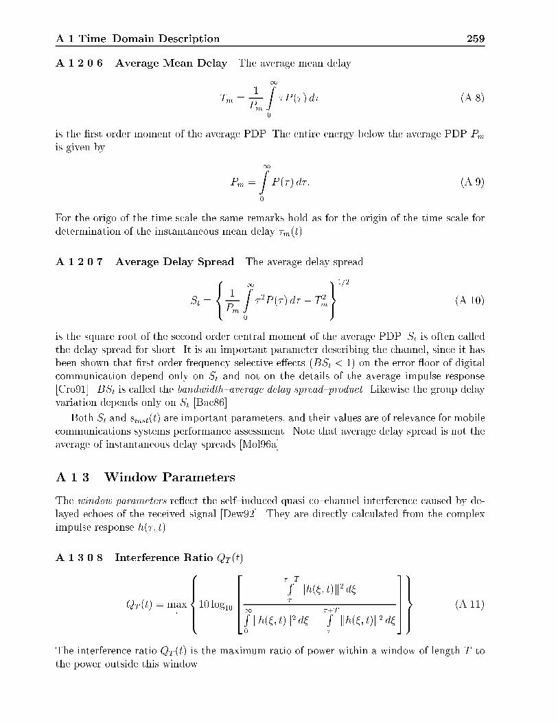
A.1 Time{Domain Description 259
A.1.2.0.6 Average Mean Delay The average mean delay
Tm =1
Pm
1Z0
�P (�) d� (A.8)
is the �rst order moment of the average PDP. The entire energy below the average PDP Pmis given by
Pm =
1Z0
P (�) d�: (A.9)
For the origo of the time scale the same remarks hold as for the origin of the time scale fordetermination of the instantaneous mean delay �m(t).
A.1.2.0.7 Average Delay Spread The average delay spread
St =
8<: 1
Pm
1Z0
� 2P (�) d� � T 2m
9=;
1=2
(A.10)
is the square root of the second order central moment of the average PDP. St is often calledthe delay spread for short. It is an important parameter describing the channel, since it hasbeen shown that �rst order frequency selective e�ects (BSt < 1) on the error oor of digitalcommunication depend only on St and not on the details of the average impulse response[Cro91]. BSt is called the bandwidth{average delay spread{product. Likewise the group delayvariation depends only on St [Bac86].
Both St and sinst(t) are important parameters, and their values are of relevance for mobilecommunications systems performance assessment. Note that average delay spread is not theaverage of instantaneous delay spreads [Mol96a].
A.1.3 Window Parameters
The window parameters re ect the self{induced quasi co{channel interference caused by de-layed echoes of the received signal [Dew92]. They are directly calculated from the compleximpulse response h(�; t).
A.1.3.0.8 Interference Ratio QT (t)
QT (t) = max�
8>>><>>>:10 log10
26664
�+TR�
kh(�; t)k2 d�1R0
kh(�; t)k2 d� ��+TR�
kh(�; t)k2 d�
377759>>>=>>>;
(A.11)
The interference ratio QT (t) is the maximum ratio of power within a window of length T tothe power outside this window.
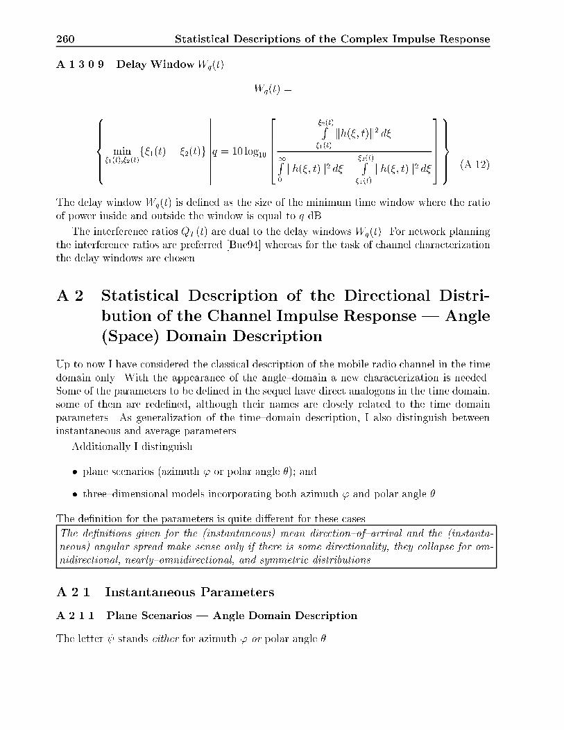
260 Statistical Descriptions of the Complex Impulse Response
A.1.3.0.9 DelayWindowWq(t)
Wq(t) =
8>>>><>>>>:
min�1(t);�2(t)
f�1(t)� �2(t)g
����������q = 10 log10
266664
�2(t)R�1(t)
kh(�; t)k2 d�
1R0
kh(�; t)k2 d� ��2(t)R�1(t)
kh(�; t)k2 d�
377775
9>>>>=>>>>; (A.12)
The delay window Wq(t) is de�ned as the size of the minimum time window where the ratioof power inside and outside the window is equal to q dB.
The interference ratios QT (t) are dual to the delay windows Wq(t). For network planningthe interference ratios are preferred [Bue94] whereas for the task of channel characterizationthe delay windows are chosen.
A.2 Statistical Description of the Directional Distri-
bution of the Channel Impulse Response | Angle
(Space) Domain Description
Up to now I have considered the classical description of the mobile radio channel in the timedomain only. With the appearance of the angle{domain a new characterization is needed.Some of the parameters to be de�ned in the sequel have direct analogons in the time domain,some of them are rede�ned, although their names are closely related to the time domainparameters. As generalization of the time{domain description, I also distinguish betweeninstantaneous and average parameters.
Additionally I distinguish
� plane scenarios (azimuth ' or polar angle �); and
� three{dimensional models incorporating both azimuth ' and polar angle �.
The de�nition for the parameters is quite di�erent for these cases.
The de�nitions given for the (instantaneous) mean direction{of{arrival and the (instanta-neous) angular spread make sense only if there is some directionality, they collapse for om-nidirectional, nearly{omnidirectional, and symmetric distributions.
A.2.1 Instantaneous Parameters
A.2.1.1 Plane Scenarios | Angle Domain Description
The letter stands either for azimuth ' or polar angle �.

A.2 Angle (Space) Domain Description 261
A.2.1.1.1 Instantaneous Directional Distribution of the Complex Impulse Re-sponse The instantaneous directional distribution of the complex impulse response
~gl(t; )�=�l (A.13)
provides a description of the angular dispersion of the scattering ensemble at a given timeinstant �l. It includes information about the positions of the scatterers.
A.2.1.1.2 Instantaneous Directional Impulse Response The instantaneous direc-tional impulse response
h(�; t; ) (A.14)
is the complex impulse response h(�; t) with additional information about the DOAs of thedi�erent paths.
A.2.1.1.3 Instantaneous Directional Power Delay Pro�le (DPDP) The instanta-neous directional PDP
Pinst(�; t; ) = kh(�; t; )k2 (A.15)
is the magnitude squared instantaneous directional impulse response. Just like its counter-part, the instantaneous PDP, Pinst(�; t), it is used for plots of h(�; t; ).
A.2.1.1.4 Instantaneous Angular Power Distribution The instantaneous angularpower distribution
Pang;inst(t; ) =
1Z�=0
Pinst(�; t; ) d� (A.16)
is a measure for the instantaneous incoming power from di�erent angles.
A.2.1.1.5 Instantaneous Mean Direction Of Arrival The instantaneous mean di-rection of arrival is de�ned as
(t) =1
Pmi
2�Z =0
Pang;inst(t; ) d : (A.17)
The mean power Pmi under the instantaneous DPDP is given by
Pmi =
1Zt=0
2�Z =0
Pang;inst(t; ) d dt: (A.18)
It can be viewed as the center of gravity of the underlying directional distribution [Egg95b].

262 Statistical Descriptions of the Complex Impulse Response
A.2.1.1.6 Instantaneous Angular Spread The instantaneous angular spread followsas
s (t) =
8><>:
1
Pmi
(t)+�Z = (t)��
2Pang;inst(t; ) d � 2(t)
9>=>;
1=2
: (A.19)
This de�nition for the instantaneous angular spread resembles the de�nition of the instanta-neous delay spread.
A.2.1.2 Three{Dimensional Scenarios | Space Domain Description
A.2.1.2.1 Instantaneous Directional Distribution of the Complex Impulse Re-sponse The instantaneous directional distribution of the complex impulse response
~gl(t; '; �)j�=�l (A.20)
provides a description of the angular dispersion of the scattering ensemble at a given timeinstant �l. It includes information about the positions of the scatterers.
A.2.1.2.2 Instantaneous Directional Impulse Response The instantaneous direc-tional impulse response
h(�; t; '; �) (A.21)
is the complex impulse response h(�; t) with additional information about the DOAs of thedi�erent paths.
A.2.1.2.3 Instantaneous Directional Power Delay Pro�le (DPDP) The instanta-neous directional PDP
Pinst(�; t; '; �) = kh(�; t; '; �)k2 (A.22)
is the magnitude squared instantaneous directional impulse response. Just like its counter-part, the instantaneous PDP, Pinst(�; t), it is used for plots of h(�; t; '; �).
A.2.1.2.4 Instantaneous Angular Power Distribution The instantaneous angularpower distribution
Pang;inst(t; '; �) =
1Z�=0
Pinst(�; t; '; �) d� (A.23)
is a measure for the instantaneous incoming power from di�erent angles.

A.2 Angle (Space) Domain Description 263
A.2.1.2.5 Instantaneous Mean Direction Of Arrival The instantaneous mean di-rection of arrival is a tuple ('(t); �(t)) given by
'(t) =
(arctan
�x(i)
y(i)
�0 if x(i) = y(i) = 0
; (A.24)
and
�(t) =
8<:
�2� arctan
�z(i)p
(x(i))2+(y(i))2
��2
if x(i) = y(i) = z(i) = 0; (A.25)
where fx; y; zg are the coordinates of the center of gravity of the underlying directionaldistribution on the sphere. These quantities are de�ned (in a cartesian) coordinate systemas the �rst order moments
x(i) =1
Pmi
ZZZS:x2+y2+z2=R2sphere
xPang;inst(t; x; y; z) dx dy dz; (A.26)
y(i) =1
Pmi
ZZZS:x2+y2+z2=R2sphere
yPang;inst(t; x; y; z) dx dy dz; (A.27)
z(i) =1
Pmi
ZZZS:x2+y2+z2=R2sphere
zPang;inst(t; x; y; z) dx dy dz; (A.28)
The integration is performed over the surface S of the sphere. Pang;inst(t; x; y; z) is the instan-taneous angular power distribution Pang;inst(t; '; �) transformed into the cartesian coordinatesystem. It can be viewed as the equivalent to the mass density function on the surface of thesphere, as used e .g. in mechanics. Of course, these integrals can be transformed into a polarcoordinate system for the purpose of analytical evaluation, therefore the instantaneous angu-lar power distribution Pang;inst(t; '; �) does not have to be really transformed into cartesiancoordinates. The angle{integrated power Pmi under the average angular power distributionis given by
Pmi =
ZZZS:x2+y2+z2=R2sphere
Pang;inst(x; y; z) dx dy dz =
2�Z'=0
�Z�=0
sin(�)Pang;inst(t; '; �) d� d':(A.29)
It can be viewed as the center of gravity of the underlying instantaneous directional distri-bution.
This de�nition di�ers from the one given in Ref. [Egg95b] since it takes into account thatthe center of gravity is in general not at the surface of the sphere.

264 Statistical Descriptions of the Complex Impulse Response
A.2.1.2.6 Instantaneous Angular Spread The instantaneous angular spread is a tuple(s'(t); s�(t)) de�ned by
s'(t) =
(arctan
�x(2;i)
y(2;i)
�0 if x(2;i) = y(2;i) = 0
; (A.30)
and
s�(t) =
8<:
�2� arctan
�z(2;i)p
(x(2;i))2+(y(2;i))2
��2
if x(2;i) = y(2;i) = z(2;i) = 0;
(A.31)
where fx(2;i); y(2;i); z(2;i)g are the second order central moments of Pang;inst(t; x; y; z). Theyare calculated as
x(2;i) =
0B@ 1
Pmi
ZZZS:x2+y2+z2=R2sphere
(x� x(i))2Pang;inst(t; x; y; z) dx dy dz
1CA
1=2
;(A.32)
y(2;i) =
0B@ 1
Pmi
ZZZS:x2+y2+z2=R2sphere
(y � y(i))2Pang;inst(t; x; y; z) dx dy dz
1CA
1=2
;(A.33)
z(2;i) =
0B@ 1
Pmi
ZZZS:x2+y2+z2=R2sphere
(z � z(i))2Pang;inst(t; x; y; z) dx dy dz
1CA
1=2
:(A.34)
Alternatively to the angular spread (S'; S�) one can also use a spatial spread (x(2;i); y(2;i); z(2;i))
to characterize the spatial propagation characteristics.
A.2.2 Average Parameters
As a function of t over a time interval, I de�ne average quantities, which are important forcharacterizing the channel.
A.2.2.1 Plane Scenarios
A.2.2.1.1 Average Directional PDP The average directional PDP
P (�; ) = EtfPinst(�; t; )g (A.35)
is a more authentic characteristic of the environment. As for the average impulse responseit can be viewed as average over frequency at a given position.

A.2 Angle (Space) Domain Description 265
A.2.2.1.2 Average Angular Power Distribution The average angular power distri-bution
Pang( ) =
1Z�=0
P (�; ) d� (A.36)
is a measure for the average incoming power from di�erent angles.
A.2.2.1.3 Average Direction Of Arrival The average direction of arrival is de�ned as
=1
Pm
2�Z =0
Pang( ) d : (A.37)
The angle{integrated power Pm under the average angular power distribution is given by
Pm =
2�Z =0
Pang( )d : (A.38)
It can be viewed as the center of gravity of the underlying average directional distribution. Iwill call it MDOA (Mean DOA) for short.
A.2.2.1.4 Average Angular Spread The average angular spread follows from
S =
8><>:
1
Pm
+�Z'=��
2Pang( ) d � 2
9>=>;
1=2
: (A.39)
Note that, as for the delay spread S, the average angular spread is not the average of themean angular spreads. I will call the average angular spread S angular spread for short.
A.2.2.2 Three{dimensional Scenarios
The signals are thought of as being incident on a sphere with Rsphere = 1. Consequently allmeasures are de�ned over that sphere.
A.2.2.2.1 Average Directional PDP The average directional PDP
P (�; '; �) = EtfPinst(�; t; '; �)g (A.40)
is a more authentic characteristic of the environment. As for the average impulse responseit can be viewed as average over frequency at a given position.

266 Statistical Descriptions of the Complex Impulse Response
A.2.2.2.2 Average Angular Power Distribution The average angular power distri-bution
Pang('; �) =
1Z�=0
P (�; '; �) d� (A.41)
is a measure for the average incoming power from di�erent angles.
A.2.2.2.3 Average Mean Direction Of Arrival The average mean direction of arrivalis a tuple (�;�) given by
� =
(arctan
�xy
�0 if x = y = 0
; (A.42)
and
� =
8<:
�2� arctan
�zpx2+y2
��2
if x = y = z = 0; (A.43)
where fx; y; zg are the coordinates of the center of gravity of the underlying directionaldistribution on the sphere. These quantities are de�ned (in a cartesian) coordinate systemas the �rst order moments
x =1
Pm
ZZZS:x2+y2+z2=R2sphere
xPang(x; y; z) dx dy dz; (A.44)
y =1
Pm
ZZZS:x2+y2+z2=R2sphere
yPang(x; y; z) dx dy dz; (A.45)
z =1
Pm
ZZZS:x2+y2+z2=R2sphere
zPang(x; y; z) dx dy dz; (A.46)
The integration is performed over the surface S of the sphere. Pang(x; y; z) is the averageangular power distribution Pang('; �) transformed into the cartesian coordinate system. Itcan be viewed as the equivalent to the mass density function on the surface of the sphere,as used e.g. in mechanics. Of course, these integrals can be transformed into a polar coor-dinate system for the purpose of analytical evaluation, therefore the average angular powerdistribution Pang('; �) does not have to be really transformed into cartesian coordinates. Theangle{integrated power Pm under the average angular power distribution is given by
Pm =
ZZZS:x2+y2+z2=R2sphere
Pang(x; y; z) dx dy dz =
2�Z'=0
�Z�=0
sin(�)Pang('; �) d� d':(A.47)
It can be viewed as the center of gravity of the underlying average directional distribution. Iwill call it MDOA (Mean DOA) for short.
This de�nition di�ers from the one given in Ref. [Egg95b] since it takes into account thatthe center of gravity is in general not at the surface of the sphere.

A.2 Angle (Space) Domain Description 267
A.2.2.2.4 Average Angular Spread The average angular spread is a tuple (S'; S�)de�ned by
S' =
(arctan
�x(2)
y(2)
�0 if x(2) = y(2) = 0
; (A.48)
and
S� =
8<:
�2� arctan
�z(2)p
(x(2))2+(y(2))2
��2
if x(2) = y(2) = z(2) = 0; (A.49)
where fx(2); y(2); z(2)g are the second order central moments of Pang(x; y; z). They are calcu-lated as
x(2) =
0B@ 1
Pm
ZZZS:x2+y2+z2=R2sphere
(x� x)2Pang(x; y; z) dx dy dz
1CA
1=2
; (A.50)
z(2) =
0B@ 1
Pm
ZZZS:x2+y2+z2=R2sphere
(z � z)2Pang(x; y; z) dx dy dz
1CA
1=2
: (A.51)
Alternatively to the angular spread (S'; S�) one can also use a spatial spread (x(2); y(2); z(2))to characterize the spatial propagation characteristics.
Note that, as for the delay spread S, the average angular spread is not the average ofthe mean angular spreads. I will call the average angular spread (S'; S�) angular spread forshort.


Appendix B
GSM{like Training Sequences for theuse with a Vectorchannel MLSE
Two typical CCI functions for the MSK{modulated GSM Training Sequences TS0{TS1 andTS0{TS2 are shown in Figure B.1a. The values for the CCF (Cross Correlation Function)both on the bit level and in the baseband domain are quite high, therefore I used two di�erenttraining sequences, which are not de�ned in the standard, namely
TSn0 : 10100001111010011010000111
TSn1 : 01111101000001010111110100: (B.1)
Their ACF and CCF are given in Figure B.1b. The cross correlation of the new sequenceswithin a time window of �4T around the optimum synchronization instant is reduced andmore uniformly distributed than in the GSM training sequences.
269

270 GSM{like Training Sequences for the use with a Vectorchannel MLSE
1 1
0.1 0.1
0 0
Normalized time shift τshift/T Normalized time shift τshift/T
Cor
rela
tion
Cor
rela
tion
CCFTS0-TS1
CCFTS0-TS2
CCFTSn0-TSn1
(a) (b)
0.2 0.2
0.3 0.3
0.4 0.4
0.5 0.5
0.6 0.6
0.7 0.7
0.8 0.8
0.9 0.9
-6 -6-4 -4-2 -20 02 24 46 6
ACFTS0
ACFTSn0
Figure B.1: ACF and CCF functions in a �ve bit interval around the optimum synchronizationinstant. (a) ACF of GSM TS0, CCF of GSM TS0{TS1 and TS0{TS2; (b) ACF of the newtraining sequence TSn0, CCF of TSn0{TSn1. The curves show that a signi�cant amount ofco{channel interference is present.

Appendix C
BER of (G)MSK
C.1 BER in an AWGN Channel
The BER for MSK with coherent detection is given by [LeM90] (Figure C.1a and C.1b)
BERcoherent = 2Q
�ds2�
��Q2
�ds2�
�; (C.1)
where ds is the distance between two signal points in the signal constellation and �2 is thenoise power. With the SNR de�ned by
SNR =a2
2�2(C.2)
and the relation
ds =p2a; (C.3)
Equation (C.1) becomes
BERcoherent = 2Q�p
SNR��Q2
�pSNR
�SNR�� 2Q
�pSNR
�= erfc
rSNR
2
!:(C.4)
Using the Viterbi algorithm for detection of the MSK{modulated signal, the squared distancedoubles, d2s;V iterbi = 2d2s [Lee73]. Therefore the BER follows as
BERcoh:;viterbi = 2Q�p
2SNR��Q2
�p2SNR
�SNR�� erfc(
pSNR): (C.5)
The BER for di�erentially coherent detected MSK is the same as for FSK [Ada89]
BERdiff:;coherent = Q
�ds2�
�= Q
�pSNR
�=
1
2erfc
rSNR
2
!: (C.6)
The BER for GMSK can be derived by considering the possible phase changes for eachpossible bit combination separately and averaging over the results. I will do that for GMSKwith BtT = 0:3, since it is used by the GSM standard. Figure C.2 shows the possible phase
271

272 BER of (G)MSK
Re{sMSK}
Im{sMSK}
bi=+1
bi=+1bi=+1
bi=+1
bi=+1
bi=-1
bi=-1
bi=-1
bi=-1
bi=-1
1
2
3
4
ds
a
1"1""1"
"-1"
"-1"
2
3
4
(b) (c)(a)
Re{sMSK}
Im{sMSK}
bi=+1
bi=-1
1
2
3
4
ds
a
Figure C.1: (a) Signal constellation for MSK. (b) Markov diagram for the use with an MLSEdetector, (c) Signal constellation for MSK for the use of a di�erentially coherent detector.
Re{sGMSK} Re{sGMSK}Re{sGMSK}
Im{sGMSK} Im{sGMSK}Im{sGMSK}
1 11
2
2
2
3
3
ds,1
ds,3
ds,2
a aa
ϕ1=90°
(a) (c)(b)
ϕ2=57.8°
3
ϕ3=30°
Figure C.2: Signal constellations for GMSK with BtT = 0:3. Only bit triplets [bn�1 bn bn+1]are considered. (a) Signal constellation for the bit triplets [1 1 1] and [-1 -1 -1]; (b) Signalconstellation for the bit triplets [1 1 -1], [- 1 1 1], [1 -1 -1], and [-1 -1 1]; (c) Signal constellationfor the triplets [1 -1 1] and [-1 1 -1].

C.2 BER in a Flat Fading Channel 273
changes that might occur during a bit duration. From [Yon88] I derive the following formulafor the phase change at the end of bit b(n),
�mod(n) = ��2b(n� 2) + ��1b(n� 1) + �0b(n) + �1b(n + 1) + �2b(n + 2);(C.7)
with ��2 = �2 = 0:2�;��1 = �1 = 15:9�;�0 = 57:8�. Since ��2 and �2 are small comparedto �1 and �0 I neglect this contribution for the analysis and focus on bit triplets only. Threedi�erent phase changes during a bit duration exist, k�mod;1k = 90�, which appears two times,k�mod;2k = 57:8�, which appears four times, and k�mod;3k = 26�, which also appears twotimes (Figure C.2). The distances ds;n; n = 1; 2; 3; are therefore given by
ds;n =
8<:
ds for n = 12 sin(57:8�)ds for n = 22 sin(30�)ds for n = 3
: (C.8)
From the ds;n's given by this formula I determine three SNRs by
SNRn =
8<:
d2=(2�2) for n = 1(2 sin(57:8�)d)2=(2�2) for n = 2(2 sin(30�)d)2=(2�2) for n = 3
(C.9)
Inserting each of these three SNRs' into Equation (C.6) and averaging over the di�erentoccurrence probabilities of the bit combinations yields
BERGMSK;diff =1
4
�Q�p
SNR1
�+ 2Q
�pSNR2
�+Q
�pSNR3
��:
(C.10)
These BERs are valid for a one{channel receiver. For a vector{channel receiver with Mchannels, like an antenna array with M elements, the sum SNR given by
SNRges =MSNR (C.11)
for the SNR on a linear scale, or, in decibel,
SNRges;dB = SNRdB + 10 log10(M); (C.12)
has to be inserted for the calculation of the BER. Taking M times the SNR for one receivechain assumes the same noise power at each antenna element and the signals at the di�erentantenna elements as fully correlated, which can be regarded as true for the investigatedmacrocell scenarios (see also the correlation functions in Chapter 2).
C.2 BER in a Flat Fading Channel
The received SNR varies in a fading channel. Therefore an averaged BER is used, which is
hBERi =1Z
=0
BER( )p( ) d ; (C.13)

274 BER of (G)MSK
where denotes the instantaneous SNR and p( ) is the PDF of the SNR.
Let
=r2
2�2(C.14)
be the instantaneous SNR with r being the Rayleigh fading signal amplitude and �2 beingthe noise power. The PDF of r is given by [Rap96]
p(r) =r
Pre�
r2
2Pr for r > 0; (C.15)
where Pr is the mean power. The PDF of the power y = r2 of the Rayleigh process followswith the use of the lemma for the transformation of PDFs [Wei91] as
p(y) =1
2Pre�
y2Pr : (C.16)
Using again the lemma for the transformation of PDFs, the PDF of the SNR follows as
p( ) =1
�e�
� ; (C.17)
with
� =Pr2�2
(C.18)
as the average SNR. Inserting Equations (C.6) and (C.17) into Equation (C.13), I get
hBERi = 1
2
1Z =0
erfc
�r
2
�1
�e�
� d : (C.19)
Performing the integration yields
hBERi =8<:
1�q
��+2
for coherent detection
12
h1�
q�
�+2
ifor di�erentially coherent detection
:(C.20)
With a Viterbi detector one gets 3dB improvement in SNR as compared to the coherentdetector. Consequently, the BER follows as
hBERiV iterbi = 1�r
�
� + 1: (C.21)
In accordance to Equation (C.9), for GMSK we have three di�erent average SNR's �1;�2,and �3. Therefore the BER with di�erentially coherent detection follows as
hBERiGMSK;diff =1
8
4�
r�1
�1 + 2� 2
r�2
�2 + 2�r
�3�3 + 2
!:
(C.22)

C.3 BER with Diversity Reception 275
C.3 BER with Diversity Reception
In the sequel I will determine the BER for diversity reception with two independently fadingpaths.
C.3.1 Selection Diversity
The BER for selection diversity with M signals is
hBERisel =
MXm=1
1Z m=0
BER( m)p( m)p( m � 1 ^ : : : ^ m � m�1 ^ m � m+1 ^ : : : ^ m � M) d m;(C.23)
where p( m � 1 ^ : : : ^ m � m�1 ^ m � m+1 ^ : : : ^ m � M) is the probability thatthe instantaneous SNR of the m{th signal, m, is larger than or equal to all other SNRs n; n = 1; 2; : : : ;M; n 6= m. I assume the fading of the signals as uncorrelated and all signalsto have the same mean power, therefore I get for the probability that all signals have an SNRless than or equal to 1
p( 1 � 2 ^ : : : ^ 1 � M) = (p( 1 � M))M�1; (C.24)
With
p( 1 � 2) =
1Z�=0
p(�) d� =
1Z�=0
1
�e�
�� d� = 1� e�
1� (C.25)
as the probability that the instantaneous SNR 1 of the �rst signal is larger than or equal tothe SNR of the second signal, 2, the sum PDF follows as
p( 1 � 2 ^ : : : ^ 1 � M) =�1� e�
1�
�M�1: (C.26)
Setting M = 2 the BER can be determined from
hBERisel =1
�
1Z =0
erfc
�r
2
�e�
�
�1� e�
�
�d
=1
2
1� 2
r�
� + 2+
r�
� + 4
!(C.27)
for MSK and
hBERisel;GMSK =1
8
4� 2
r�1
�1 + 2+
r�1
�1 + 4� 4
r�2
�2 + 2
+2
r�2
�2 + 4� 2
r�3
�3 + 2+
r�3
�3 + 4
!(C.28)
for GMSK with di�erentially coherent detection.

276 BER of (G)MSK
C.3.2 Maximal Ratio Combining (MRC)
The PDF of the SNR after applying MRC is given by [Jak74]
p( ) = M�1e�
�
�M(M � 1)!; � 0: (C.29)
Therefore the BER follows as
hBERiMRC =1
2�M(M � 1)!
1Z =0
M�1e� � d : (C.30)
Setting M=2, I get
hBERiMRC =1
2
1� �(6 + 2�)p
2(2 + �)p2�(2 + �)
!(C.31)
for MSK and
hBERiMRC;GMSK =1
8
4� �1(6 + 2�1)p
2(2 + �1)p2�1(2 + �1)
� 2�2(6 + 2�2)p
2(2 + �2)p2�2(2 + �2)
� �3(6 + 2�3)p2(2 + �3)
p2�3(2 + �3)
!(C.32)
for GMSK with di�erentially coherent detection.

Appendix D
Probability of Estimation Errors ofthe Channel Impulse Response due toCCI
In Figure B.1b the CCI level present for channel impulse response estimation due to a non{zero cross correlation between the training sequences can be seen. The maximum of the CCFis 1=8 times the maximum of the ACF. Consequently, if the channel impulse response for oneuser is in amplitude below 1=8 of the amplitude of the channel impulse response of the otheruser, the estimated channel impulse response for the �rst user (channel) would be completelydisturbed by CCI. The BER for this user would be 0:5 for the corresponding data slot.
Without loss of generality I assume the �rst channel to be the one with the lower ampli-tude. The simulated MLSE considers impulse responses of length LMLSE = 3 (one symbolbefore and one symbol after the main pulse), so the �rst channel constellation, where theestimation accuracy of the impulse response for the �rst user is impaired, is given by thecondition
3a1 = a2 (D.1)
for the amplitudes of the �rst and the second channel, respectively, and
�1 = � + �2 (D.2)
for the phases of the two channels, where �k; k = 1; 2; denotes the phase of the k{th channel.Only two ([-1 1 -1], [1 -1 1]) out of eight possible bit combinations are in error, consequentlythe BER is 0.25. The channel constellations, where errors occur, increase with decreasingamplitude of the �rst path down to 8a1 = a2, where the situation mentioned at the beginningis found. To take this into account I distinguish between two di�erent regions | Region 1(8a1 � a2) and Region 2 (3a1 � a2 � 8a1). In the following let A = 8 and B = 3.
The probability for the �rst channel to be in amplitude within 1=A to 1=B times theamplitude of the second channel is
p�a2A� a1 � a2
B
�=
r=AZr1=r=B
r1Pre�
r212Pr dr1 = e
� r2
2PrA2 � e� r2
2PrB2 : (D.3)
277

278 Estimation Errors due to CCI
For Region 1 this PDF is given by
p(0 � a1 � a2=A) = 1� e� r2
2PrA2 : (D.4)
For Region 1 the probability of occurrence of a channel constellation with 0 � a1 � a2=Afollows therefore as
pRegion1 =
1Zr=0
r
Pr
�1� e
� r2
2PrA2
�e�
r2
2Pr dr =1
1 + A2: (D.5)
Since the error rate over all bit triplets for these channel constellations is 0:5, the total BERfor Region 1 due to non{orthogonal training sequences follows as
BERRegion1 =1
2(1 + A2): (D.6)
For Region 2 the probability of occurrence of a channel constellation with a2=A � a1 � a2=Bis given by
pRegion2 =
1Zr=0
r
Pr
�e� r2
2PrA2 � e� r2
2PrB2
�e�
r2
2Pr dr =A2
1 + A2� B2
1 +B2: (D.7)
As explained above, not all channel constellations lead to errors in Region 2, it depends onthe phase di�erence between the two channels. The number of constellations, where errorsoccur, increase linearly from zero (for a1 = a2=B) to one (for a1 = a2=A). I take this e�ectinto account by taking only half of the channel constellations into account for the BERcalculation. The error rate over all bit triplets is 0.25, therefore the total BER for Region 1due to non{orthogonal training sequences follows as
BERRegion2 =1
8
�A2
1 + A2� B2
1 +B2
�: (D.8)
With these results the total bit error rate in a Rayleigh{fading channel due to non{orthogonaltraining sequences follows as
BERCCI =1
2(1 + A2)+1
8
�A2
1 + A2� B2
1 +B2
�: (D.9)
If I insert the speci�c values for A and B, I get
BERCCI = 1:83:10�2; (D.10)
which �ts well with the value derived from the simulations (Figures 5.3, 5.4).

Appendix E
BER for a User Disturbed byCo{Channel Interference Having theSame Modulation and the Same MeanPower
Consider two bipolar bit streams fmk;ngNn=1 2 f�1; 1g; k = 1; 2 to be transmitted over afading channel without noise. The �rst bit stream represents the desired signal, the secondthe interfering signal. Assume that both signals are incident at the receive antenna of aconventional mobile radio receiver (which detects only one bit stream) at the same timeinstant, with equal mean power, and are subjected to uncorrelated fading.
Let m1;n be the n{th bit detected by a di�erential detector. Now there are two possibilities
1. m1;n = m2;n: Then m1;n = m1;n, i.e. the BER is zero, BER1 = 0.
2. m1;n 6= m2;n: The BER is zero (m1;n = m1;n) if p1 � p2 and one (m1;n 6= m1;n) if p1 < p2.pk; 1 � k � 2 denotes the instantaneous power of the k{th path. The relative phaseof the two paths has no in uence on the BER, since I assume a di�erential detector.Since both signals have the same mean power and are subjected to uncorrelated fading,p1 � p2 has the same probability as p2 � p1. Averaging gives BER2 =
12(0 + 1) = 0:5.
The average BER is now given by
BER =1
2(BER1 + BER2) = 0:25: (E.1)
279


Appendix F
Spatial Separability of VariousIncident Signals
Assume, that K waves with DOAs f'1; '2; : : : ; 'k; : : : ; 'Kg are incident on a 1D{ULA withM elements with a normalized spacing of d=�. I now want to �nd a measure for the spatialseparability �ges of this scenario.
As measure for the spatial separability of two incident signals I de�ne in accordance with[Far96b]
�k1;k = dist2(a('k1);a('k)) = 1��
1
ka('k1)kka('k)ka('k1)
Ha('k)
�2
2 [0; 1];(F.1)
which is simply the squared distance dist(:) between the subspaces spanned by the twosteering vectors a('k1);a('k) in an Euclidean space as de�ned in [Gol83].
The array steering vector a('k) is de�ned in the usual way as
a('k) = [1; e�j2�d sin('k)=�; : : : ; e�j2�(M�1)d sin('k)=�]T ; (F.2)
i.e. the separability �k1;k and consequently the overall spatial separability �ges depend bothon the incidence angles of the considered signals and on the size of the BS antenna. Theoverall spatial separability �ges is now given by
�ges = minf�k1;kg; k1; k = 1; 2; : : : ; K; k1 6= k: (F.3)
If �ges > 0:9 I call a scenario well separable, otherwise it is called poorly separable.
Figure F.1 shows the spatial separability for two incident signals versus their DOAs. Inthe diagonal the separability is zero, since there the DOA of the two signals is the same.
Since only the angle di�erence of the incident signals and the size of the antenna arrayin uence the spatial separability, one can also use the term angular separability for �.
281

282 Spatial Separability
−500
50
−500
50
0
0.2
0.4
0.6
0.8
16
�ges
QQQQk
'1 (deg)��
���1
'2 (deg)
Figure F.1: Spatial separability �ges versus the DOA of two incident signals for a 1D{ULAwith M = 8 and d=� = 0:5.

Appendix G
Null Broadening Algorithm forKnown DOAs
Here I summarize the null broadening algorithm as introduced in Ref. [Ger96]. Let usassume, that I want to broaden all the nulls in the downlink antenna pattern for the lk{thpath of user k, where it points into the direction of another signal (user). This problem canbe stated as the following conditional maximization problem
maxwd;k;lk
kwTd;k;lk
a('k;lk)k2 (G.1)
wTd;k;lk
a('k1;lk1 ) = 0; k1 = 1; 2; : : : ; K; k1 6= k (G.2)
@p(wTd;k;lk
a('))
@�p
���'='k1;lk1 = 0 ; k1 = 1; 2; : : : ; L1 + L2 + : : :+ LK ; k1 6= k
p = 1; 2; : : : ; PNB; � = (2�=�) sin(') (G.3)
wHd;k;lk
wd;k;lk = 1; (G.4)
where (L1 + L2 + : : : + LK � 1)(PNB + 1) < M has to be guaranteed. Since in mobilecommunications M is rather small, PNB is small too, i.e. typically PNB = 1; 2. Physically,Equation G.3 implies the nulls to be at, i.e. that PNB of the higher order derivatives arezero for the locations of the nulls. In the following I assume the array to be well calibrated,i.e. the antenna positions are known. In the case of imperfectly calibrated arrays, usuallythe more robust phase{independent derivative constraints should be used [Tse92].
Now, we construct theM�M diagonal matrix of the coordinates of the antenna elementsas
Be = diagfx1; x2; : : : ; xm; : : : ; xMg; (G.5)
where xm is the coordinate of the m{th antenna element in meters. We now form the matrix
F k;lk = [Adown;k;lk;BeAdown;k;lk; : : : ;BPNBe Adownk;lk]; (G.6)
283

284 Null Broadening Algorithm for Known DOAs
where the altered array steering matrix Adown;k;lk is given by
Adown;k;lk = [a('1;1); : : : ;a('k;lk�1);a('k;lk+1); : : : ;a('K;lK)]; (G.7)
i.e. the (k; lk){th column (which is the steering vector for the desired signal) is omitted.
As shown in Ref. [Ger96] the solution to the optimization problem stated at the beginningis given by
wd;k;lk =1q
a('k;lk)HDk;lka('k;lk)
Dk;lka('k;lk); (G.8)
where Dk;lk is a projection matrix given by
Dk;lk = IM � F k;lk(FHk;lkF k;lk)
�1FHk;lk; (G.9)
where IM is the (M �M) identity matrix.
This procedure works only for weight vectors to be derived by WSA, since it assumes eachsteering vector a('k;lk) to contain only one DOA.

Appendix H
List of Frequently Used Acronyms
285

286 List of Frequently Used Acronyms
Acronym Description
1D{ULA one{Dimensional Uniform Linear Array4QAM 4 Quadrature AmplitudeModulation4xS Single Snapshot Spatial SeparationACF AutoCorrelation FunctionAIC An Information CriterionA{SDMA Adaptive Space Division Multiple AccessATAM2E Adaptive Transmitting Antenna Methods for
Multipath EnvironmentsBA Bayesian ArraysBCCH Broadcast Control CHannelBEMCCS Blind Estimation of Multiple Co{Channel SignalsBER Bit Error RateBS Base StationBSC Base Station ControllerBSS Base Station SystemBTS Base Transceiver StationCCEI Correlative Channel Estimation in the presence of both users
and InterferenceCCEN Correlative Channel Estimation in the presence
of the desired user and Noise onlyCCENI Correlative Channel Estimation in the presence of both users
with Noise and InterferenceCCF Cross Correlation FunctionCCI Co{Channel InterferenceCDF Cumulative Distribution FunctionCDMA Code DivisionMultiple AccessCIR Carrier to Interference RatioCMA Constant Modulus AlgorithmCMCS CellularMobile Communications SystemCOST European Cooperation in the Field Of Scienti�c and Technical ResearchCS/SR Correlation{based Synchronization for Spatial Reference algorithmsCS/TR Correlation{based Synchronization for Temporal Reference algorithmsCT Cordless TelephoneD{AMPS Digital Advanced Mobile Phone SystemDB Digital BeamformingDBST Downlink Beam Steering TechniqueDCA Dynamic Channel AllocationDCS1800 Digital Communications System at 1800MHzDDC Digital Down ConversionDECT Digital Enhanced Cordless TelecommunicationsDFA Decision Feedback ArrayDMI Direct Matrix Inversion

287
Acronym Description
DOA Direction{Of{ArrivalDPDP Directional Power Delay Pro�leDQPSK Di�erential Quadrature Phase Shift KeyingDRA Dynamic Resource AllocationDSP Digital Signal ProcessingEIA Electronic Industry AssociationESPRIT Estimation of Signal Parameters via Rotational Invariant TechniquesETSI European Telecommunications Standardization InstituteFACCH Fast A1ssociated Control CHannelFBLP Forward Backward Linear PredictionFDBA Farsakh's Downlink Beamforming AlgorithmFDD Frequency Division DuplexFDMA Frequency DivisionMultiple AccessFRLS Fast Recursive Least SquaresGLPF Gaussian LowPass FilterGMSK Gaussian Minimum Shift KeyingGSM Global System for Mobile CommunicationsHCS Hierarchical Cell StructuresIMT{2000 International Mobile Telecommunications System 2000IS{95 EIA Interim Standard for U.S. code division multiple accessISI InterSymbol InterferenceITU International Telecommunications UnionJSA Joint Synchronization and AdaptationLMS Least Mean SquaresLOS Line Of SightLS Least SquaresLSCENI Least Squares Channel Estimation in the presence of
both users with Noise and InterferenceMAVT Mobile Audio Visual TerminalMDL Minimum Description LengthMDOA Mean Direction{Of{ArrivalMLLMSAP Maximum Likelihood Localization of Multiple Sources by
Alternating ProjectionMLSE Maximum Likelihood Sequence EstimatorMRC Maximal Ratio CombinerMS Mobile StationMSE Mean Squared ErrorMSK Minimum Shift KeyingMtBFB Mobile to Base FeedBackMUSIC MUltiple Signal Classi�cationNLOS Non Line Of SightNMT Nordic Mobile Telephone

288 List of Frequently Used Acronyms
Acronym Description
PCH Paging CHannelPDF Probability Density FunctionPDP Power Delay Pro�lePHS Personal Handyphone SystemRABW Recursive Adaptive Beamforming for Wireless CDMARACE Research and development in Advanced Communications in EuropeRACH Random Access CHannelRBF Radial Basis FunctionRF Radio FrequencyRLL Radio Local LoopRLS Recursive Least SquaresRoE Ratios of EigenvaluesSAGE Space{Alternating Generalized Expectation|maximum algorithmSDCCH Slowly Dedicated Control CHannelSFIR Spatial Filtering for Interference ReductionSFU Spatial Filtering at the Uplink onlySIR Signal to Interference RatioSMG{5 Special Mobile Group 5SMI Sampled Matrix InversionSNIR Signal to Noise and Interference RatioSNIR/SR Signal to Noise and Interference Ratio | based synchronization for
Spatial Reference algorithmsSNR Signal{to{Noise RatioSOI Signal Of InterestSQRLS Square Root Recursive Least SquaresSR Spatial ReferenceST{AWGN Spatio{Temporal Additive White Gaussian NoiseSTD Space{Time DecompositionSTD{SIMI Space{Time Decomposition | SIngle Matrix InversionSVD Singular Value DecompositionSWA Sum and Weight AlgorithmTA2WC Blind Adaptive Transmission Antenna Algorithm for
Wireless CommunicationTACS Total Access Communications SystemTAM Toeplitz Approximation MethodTCH Tra�c CHannelTCH/F Tra�c CHannel Full{rateTDD Time Division DuplexTDMA Time DivisionMultiple AccessTR Temporal ReferenceTS Training Sequence

289
Acronym Description
TSUNAMI Technology in Smart Antennas forUNiversal Mobile Infrastructure
UCA{ESPRIT Uniform Circular Array { Estimation of Signal Parametersvia Rotational Invariant Techniques
UMTS Universal Mobile Telecommunications SystemUPT Universal Personal TelecommunicationsVIASS Virtual{Image{Array Single Snapshot algorithmWLAN Wireless Local Area NetworksWLL Wireless Local LoopW{PBX Wireless Private Branch eXchangeWSA Weight and Sum AlgorithmWSF Weighted Subspace FittingZTA Zetterberg's Transmission Algorithm

290 List of Frequently Used Acronyms

Appendix I
List of Frequently Used Symbols
Lower{case italic letters denote variables, upper{case italic letters denote constants, bothcan be real or complex valued. Vectors are denoted by lower{case boldface letters, whereasmatrices are denoted by upper{case boldface letters. (:)� denotes complex conjugate (withouttransposition), (:)T denotes transpose, (:)H denotes hermitean transpose, i.e. transpose and
conjugate complex, (:)+ denotes the Moore{Penrose pseudoinverse. (:) denotes an estimateof the corresponding quantity (:). X(:; l : k) (X(l : k; :)) stands for the l{th to k{th column(row) of the matrix X .
291

292 List of Frequently Used Symbols
Symbol Description Section
Q co{channel reuse ratio 1.2Rf cell radius 1.2Df distance between two co{channel cells 1.2
H(�; t) impulse response matrix 2.1hkm(�; t) instantaneous complex impulse response for transmission 2.1
from the k{th user to the m{th antenna element� delay time 2.1t absolute time 2.1gl;km(t) amplitude of the l{th path 2.1�(:) Dirac's delta pulse 2.1~gl;MS(t; '; �) instantaneous directional distribution of the 2.1
channel impulse response at the MS~gl;BS(t; '; �) instantaneous directional distribution of the 2.1
channel impulse response at the BS� elevation angle 2.1' azimuthal angle 2.1hMS(�; t; '; �) instantaneous directional impulse response at the MS 2.1hBS(�; t; '; �) instantaneous directional impulse response at the BS 2.1
r(M)l distance from the mobile to the l{th scatterer 2.1
r(l)m distance from the l{th scatterer to the m{th antenna element 2.1ale
j�l scattering coe�cient of the l{th scatterer 2.1~vMS velocity vector of the MS 2.1'vMS
angle of the velocity vector of the MS 2.1� wavelength 2.1'l;BS azimuthal angle under which the l{th scatterer 2.1
is seen from the BS'l;MS azimuthal angle under which the l{th scatterer 2.1
is seen from the MS� power attenuation exponent 2.1f0 carrier frequency 2.1c0 velocity of light 2.1P (�; t) power delay pro�le A.1h(�; x); h(�; t) instantaneous complex impulse response A.1Pinst(�; t) instantaneous power delay pro�le A.1�m(t) instantaneous mean delay A.1Pmi mean power of the PDP A.1sinst(t) instantaneous delay spread A.1P (�) average power delay pro�le A.1Etf:g average over t A.1Tm average mean delay A.1Pm energy below the average PDP A.1St average delay spread A.1

293
Symbol Description Section
QT (t) interference ratio A.1Wq(t) delay window A.1~gl(t; '; �)j�=�l instantaneous directional distribution A.1
of the complex impulse responseh(�; t; '; �) instantaneous directional impulse response A.1Pinst(�; t; '; �) instantaneous directional PDP A.1Pang;inst(t; '; �) instantaneous angular power distribution A.1
('(t); �(t)) instantaneous mean direction of arrival A.1(s'(t); s�(t)) instantaneous angular spread A.1P (�; '; �) average directional PDP A.1Pang('; �) average angular power distribution A.1
(�;�) average mean direction of arrival A.1(S'; S�) average angular spread A.1Bfilter receiver �lter bandwidth 2.2'3dB 3dB beamwidth of the antenna pattern in azimuth 2.2�3dB 3dB beamwidth of the antenna pattern in elevation 2.2x output signal vector of the BS antenna array 2.2n(�) ST{AWGN vector 2.2s(�) vector containing the transmitted signals from the mobile 2.2� angular width of the scatterer scenario as seen frm the BS 2.3R radius of the scatterer circle 2.3rMS distance between BS and MS 2.3p';k('l) PDFs of the azimuthal angular distribution 2.3
of the scatterersQk normalizing constant 2.3�� standard deviation of the spread{out DOAs 2.3erf(a) real{valued error function 2.3F (:) cumulative distribution function 2.3p(:) probability density function 2.3r1 inner cell radius 2.3r2 outer cell radius 2.3!0 radian center frequency 2.3sr;m(�) received signal at the m{th antenna 2.3�gnl;1m terms comprising gl;1m 2.3
� (m)nl delay of the nl{th signal arriving at element m 2.3
�(m)nl equivalent phase shift 2.3
�lm di�erence in pathlength between the scatterer 2.3and two antenna elements
d distance between two antenna elements 2.3xl;1m real part of gl;1m 2.3yl;1m imaginary part of gl;1m 2.3j complex unity 2.3

294 List of Frequently Used Symbols
Symbol Description Section
~�xx real part of the correlation coe�cient 2.3~�xy imaginary part of the correlation coe�cient 2.3�2s sum power of the paths 2.3Jk(
:) Bessel function of integer order k 2.3A(a; b) di�erence of the two real parts of erf(a) and erf(b) 2.3B(a; b) di�erence of the two imaginary parts of erf(a) and erf(b) 2.3erf(a + jb) complex{valued error function 2.3w(x) complex probability function 2.3�env envelope correlation coe�cient 2.3xrm;!1 real part of the signal srm;!1 at frequency !1 2.3yrm;!1 imaginary part of the signal srm;!1 at frequency !1 2.3~�xx;�! frequency correlation coe�cient of 2.3
the real part of the signal~�xy;�! frequency correlation coe�cient of the 2.3
imaginary part of the signal�� phase di�erence 2.3r radius of the scatterer ring 2.3�r;�! sum correlation coe�cient 2.3gLOS amplitude of the LOS component of the received signal 2.3gLOS (linear) mean value of the received LOS amplitude 2.3�LOS standard deviation of the LOS signal amplitude 2.3ln(:) natural logarithm 2.3h(�) �lter impulse response 2.3rln(gLOS)(�) ACF of ln(gLOS) 2.3rd(i) exponential correlation model 2.3i discrete{time variable 2.3� continuous valued space variable 2.3�r shape parameter 2.3C normalization factor 2.3KRice(dB) Rice{factor 2.3�'s separation between the local scatterers 2.3
and the distant scatterersNs number of local scatterers 2.4Ndiscr number of discrete re ectors 2.4wStreet street width 2.4wRoom room width 2.4
R(�) periodic cross{correlation function 3.1of two training sequences
PTr number of distinct training sequences 3.1S length of the training sequences 3.1hPB(�) impulse response of the passband �lter 3.1hBB(�) impulse response of the baseband �lter 3.1
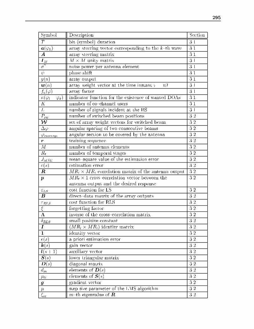
295
Symbol Description Section
T bit (symbol) duration 3.1a('k) array steering vector corresponding to the k{th wave 3.1A array steering matrix 3.1IM M �M unity matrix 3.1�2 noise power per antenna element 3.1 phase shift 3.1y(n) array output 3.1w(n) array weight vector at the time instant � = nT 3.1fn(') array factor 3.1�('l � 'k) indicator function for the existence of wanted DOAs 3.1K number of co{channel users 3.1L number of signals incident at the BS 3.1Psw number of switched beam positions 3.2W set of array weight vectors for switched beam 3.2�' angular spacing of two consecutive beams 3.2'coverage angular section to be covered by the antenna 3.2r training sequence 3.2M number of antenna elements 3.2Rt number of temporal stages 3.2JMSE mean{square value of the estimation error 3.2e(s) estimation error 3.2R MRt �MRt correlation matrix of the antenna output 3.2p MRt � 1 cross{correlation vector between the 3.2
antenna output and the desired response"LS cost function for LS 3.2B direct{data matrix of the array outputs 3.2"RLS cost function for RLS 3.2� forgetting factor 3.2� inverse of the cross{correlation matrix 3.2�RLS small positive constant 3.2I (MRt �MRt) identity matrix 3.21 identity vector 3.2e(s) a priori estimation error 3.2k(s) gain vector 3.2l(s+ 1) auxiliary vector 3.2S(s) lower triangular matrix 3.2D(s) diagonal matrix 3.2dm elements of D(s) 3.2�li elements of S(s) 3.2g gradient vector 3.2� step size parameter of the LMS algorithm 3.2�m m{th eigenvalue of R 3.2

296 List of Frequently Used Symbols
Symbol Description Section
� diagonal matrix containing the ordered eigenvalues of R 3.2�2 delay of the second wavefront R 3.2JCMA cost function of the CMA algorithm 3.2pCMA; qCMA integers 3.2�CMA input constant modulus 3.2sign(:) signum{function 3.2u(d) signal canceller weight vector 3.2e(d) error signal vector at time instant � = dT 3.2Br direct data matrix of the r{th stage 3.2wr weight vector of the r{th stage 3.2yr(n) output signal of the r{th stage at time instant � = nT 3.2yRt(n) vector of the outputs of the Rt stages 3.2SNR vector containing the SNR's 3.2Bc truncated direct data matrix 3.2rr truncated version of the training sequence 3.2F K �K state transition matrix 3.2
(�)m K � 1 state vector 3.2
of the sensor element m at time �H direct data matrix 3.2�1 diagonal matrix containing the M singular values 3.2U 1 left singular vectors spanning the signal subspace 3.2U 2 left singular vectors spanning the noise subspace 3.2V 1 right singular vectors spanning the signal subspace 3.2V 2 right singular vectors spanning the noise subspace 3.2�; factorization matrices 3.2
�# factorization matrix � without the last row 3.2
�" factorization matrix � without the �rst row 3.2
pf(K) free (adjustable) parameters in the estimate 3.2
of the covariance matrix R�s
1 diagonal matrix containing the estimates 3.2of the eigenvalues
W estimated weighting matrix 3.2Rfb forward{backward averaged covariance matrix 3.2Rb backward covariance matrix 3.2
x(b)(d) backward array data vector 3.2E permutation matrix 3.2sr amplitude of the resolved signal 3.2snr amplitude of the non{resolved signal 3.2~x(n) extended data vector 3.2~w(n) extended weight vector 3.2D1 length of the feedback �lter 3.2wBd(n) d{th coe�cient of the feedback �lter 3.2

297
Symbol Description Section~B extended direct{data matrix 3.2P (�ijx) a posteriori probability of class �i 3.2
assuming the array output xpx(xj�i) conditional probability density function of x 3.2Pi a priori probability of class �i 3.2p(x) probability density function of the array output vector x 3.2z(h) node output 3.2c center 3.2Rn noise correlation matrix 3.2f(:) exponential function 3.2�RBF width of f(:) 3.2Hw(j!) transfer function of the noise{whitening �lter 3.2Nmod number of possible symbols in the data to be transmitted 3.2Lchannel memory of the channel normalized to a symbol duration T 3.2Nh number of samples belonging to node class Kh 3.2z(n) output vector of the hidden layer 3.2Z direct{data matrix of the outputs of the hidden layer 3.2w(RBF )(n) coe�cient vector for the output layer 3.2S(j!) spectrum of the transmitted signal s(�) 3.2xh(n) hypothesis symbol 3.2Dn branch metric 3.2�k(n) state of a single{user single{channel MLSE 3.2�k(n) superstate for the multiple{user vectorchannel MLSE 3.2
hm (KLchannel � 1) vector of the impulse responses for 3.2transmission from the K users to the m{th antenna element
xm;sum sum data vector 3.2RTr block circulant matrix containing the 3.2
training sequences for the K users
hkm;corr correlative estimate of the impulse response for 3.2transmission from the k{th user to the m{th antenna element
�o timing o�set 3.2
bk(n) n{th bit of the k{th user 4.1sc(�) complex RF{signal 4.1sBB(�) complex envelope 4.1SBB constant envelope of the signal 4.1�0 initial phase 4.1�mod(�) excess phase 4.1!m angular frequency shift 4.1pD(�) bipolar sequence of data pulses 4.1Bt 3dB bandwidth of the GLPF 4.1
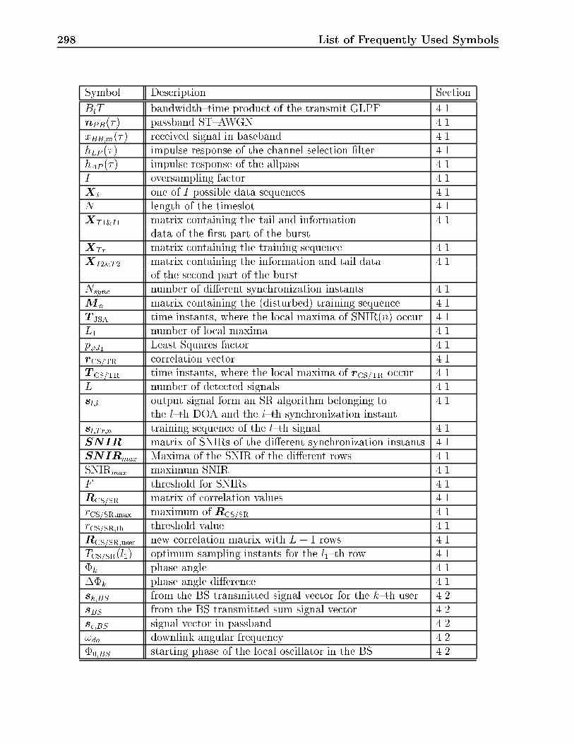
298 List of Frequently Used Symbols
Symbol Description Section
BtT bandwidth{time product of the transmit GLPF 4.1nPB(�) passband ST{AWGN 4.1xBB;m(�) received signal in baseband 4.1hLP (�) impulse response of the channel selection �lter 4.1hAP (�) impulse response of the allpass 4.1I oversampling factor 4.1X i one of I possible data sequences 4.1N length of the timeslot 4.1XT1&I1 matrix containing the tail and information 4.1
data of the �rst part of the burstXTr matrix containing the training sequence 4.1XI2&T2 matrix containing the information and tail data 4.1
of the second part of the burstNsync number of di�erent synchronization instants 4.1Mn matrix containing the (disturbed) training sequence 4.1T JSA time instants, where the local maxima of SNIR(n) occur 4.1L1 number of local maxima 4.1p';l1 Least Squares factor 4.1rCS=TR correlation vector 4.1T CS=TR time instants, where the local maxima of rCS=TR occur 4.1L number of detected signals 4.1sl;i output signal form an SR algorithm belonging to 4.1
the l{th DOA and the i{th synchronization instantsl;T r;n training sequence of the l{th signal 4.1SNIR matrix of SNIRs of the di�erent synchronization instants 4.1SNIRmax Maxima of the SNIR of the di�erent rows 4.1SNIRmax maximum SNIR 4.1F threshold for SNIRs 4.1RCS=SR matrix of correlation values 4.1rCS=SR;max maximum of RCS=SR 4.1rCS=SR;th threshold value 4.1RCS=SR;user new correlation matrix with L� 1 rows 4.1TCS=SR(l1) optimum sampling instants for the l1{th row 4.1�k phase angle 4.1��k phase angle di�erence 4.1sk;BS from the BS transmitted signal vector for the k{th user 4.2sBS from the BS transmitted sum signal vector 4.2sc;BS signal vector in passband 4.2!do downlink angular frequency 4.2�0;BS starting phase of the local oscillator in the BS 4.2

299
Symbol Description Section
BER bit error rate 5.0'min minimum distance between the incident signals of two users 5.0�'max�null distance between the maximum and the �rst null 5.0
of a broadside antenna patternSNRlin SNR at one antenna element on a linear scale 5.1SNRs;lin sum SNR on a linear scale 5.1�' angle between two co{channel users 5.2�'DOA angular width of the clustering region 6.1V number of DOAs within a predetermined 6.1
angular region �'DOAzmm self impedance 6.1zmk mutual impedance 6.1Pk power of the k{th user incident at the reference element 6.1Mc number of elements of the circular array 7.1Mt number of elements of one 1D{ULA of the triangular topology 7.1Ms number of elements of one 1D{ULA of the quadratic topology 7.1f(�) vertical radiation pattern of one antenna element 7.1wd;k downlink weight vector for the k{th user 8.1Lk number of DOAs for the k{th user 8.1SNIRup matrix with SNIRs determined from the uplink 8.1DOAup matrix with DOAs determined from the uplink 8.1
SNIRup mean values of the uplink SNIRs 8.1
DOAup mean values of the uplink DOAs 8.2rk;lk steering vector for the lk{th propagation path 8.2
for the k{th userAdown downlink array steering matrix 8.3�d wavelength at the downlink frequency 8.3W down downlink array weight matrix 8.3~Adown modi�ed array steering matrix 8.3Nu size of the averaging window 8.4PNB null broadening parameter 8.4Sf number of duplex channels 9.1sf number of channels allocated to one cell 9.1Ncl cluster size 9.1Ff frequency reuse factor 9.1Q co{channel reuse ratio 9.1Se spectral e�ciency 9.1A totally o�ered tra�c 9.1Fcell cell area 9.1
�CIR di�erence of the mean CIR 9.1

300 List of Frequently Used Symbols
Symbol Description Section
Pout outage probability 9.1�CIR5% di�erence of the CIR at the 5%{level of Pout 9.1rMS;0 distance for reference point 9.1P0 reference power 9.1�' standard deviation of the pointing error 9.2�PC standard deviation of the power control error 9.2� Power range in a cell 9.2rc+1; rc radii of power class c 10.1pmax maximum power of the accepted user 9.1pmin minimum power of the accepted user 9.1PL maximum path loss permitted for one power class 10.1
ds distance between two signal points C.1in the signal constellation
a amplitude of the point in the signal constellation C.1Pr mean power of the Rayleigh process C.2 instantaneous SNR C.2� mean SNR C.2�i; i = 1; 2; 3 mean SNRs for GMSK (BtT = 0:3) C.2LMLSE length of the impulse responses considered by the MLSE Dai; i = 1; 2 amplitude of the impulse response of the i{th user D�i; i = 1; 2 phase of the impulse response of the i{th user D
Adown;k;lk altered array steering matrix D
B M �M diagonal matrix containing the coordinates Gof the antenna elements
F k;lk matrix containing the conditions Gfor the null broadening algorithm
Dk;lk projection matrix G
fmk;ngNn=1; k = 1; 2 bipolar bit stream E
�k1;k spatial separability of the two signals with index k1 and k F�ges overall spatial separability F

Appendix J
List of Frequently Used Symbols |Alphabetically Ordered
Lower{case italic letters denote variables, upper{case italic letters denote constants, bothcan be real or complex valued. Vectors are denoted by lower{case boldface letters, whereasmatrices are denoted by upper{case boldface letters. (:)� denotes complex conjugate (withouttransposition), (:)T denotes transpose, (:)H denotes hermitean transpose, i.e. transpose and
conjugate complex, (:)+ denotes the Moore{Penrose pseudoinverse. (:) denotes an estimateof the corresponding quantity (:). X(:; l : k) (X(l : k; :)) stands for the l{th to k{th column(row) of the matrix X .
301

302 Frequently Used Symbols | Alphabetically Ordered
Symbol Description Section
1 identity vector 3.2A array steering matrix 3.1Adown downlink array steering matrix 8.3Adown;k;lk altered array steering matrix D~Adown modi�ed array steering matrix 8.3A totally o�ered tra�c 9.1a('k) array steering vector corresponding to the k{th wave 3.1a amplitude of the point in the signal constellation C.1ai; i = 1; 2 amplitude of the impulse response of the i{th user Dale
j�l scattering coe�cient of the l{th scatterer 2.1A(a; b) di�erence of the two real parts of erf(a) and erf(b) 2.3B direct{data matrix of the array outputs 3.2Bc truncated direct data matrix 3.2Be M �M diagonal matrix containing the coordinates G
of the antenna elementsBr direct data matrix of the r{th stage 3.2~B extended direct{data matrix 3.2BER bit error rate 5.0Bfilter receiver �lter bandwidth 2.2Bt 3dB bandwidth of the GLPF 4.1BtT bandwidth{time product of the transmit GLPF 4.1B(a; b) di�erence of the two imaginary parts of erf(a) and erf(b) 2.3bk(n) n{th bit of the k{th user 4.1C normalization factor 2.3c center 3.2c0 velocity of light 2.1D(s) diagonal matrix 3.2Dk;lk projection matrix G
DOAup matrix with DOAs determined from the uplink 8.1
DOAup mean values of the uplink DOAs 8.2D1 length of the feedback �lter 3.2Df distance between two co{channel cells 1.2
Dn branch metric 3.2d distance between two antenna elements 2.3dm elements of D(s) 3.2ds distance between two signal points C.1
in the signal constellationE permutation matrix 3.2Etf:g average over t A.1e(d) error signal vector at time instant � = dT 3.2

303
Symbol Description Section
e(s) (a priori) estimation error 3.2erf(a) real{valued error function 2.3erf(a + jb) complex{valued error function 2.3F K �K state transition matrix 3.2F k;lk matrix containing the conditions G
for the null broadening algorithmF threshold for SNIRs 4.1Fcell cell area 9.1Ff frequency reuse factor 9.1F (:) cumulative distribution function 2.3f(:) exponential function 3.2f0 carrier frequency 2.1fn(') array factor 3.1f(�) vertical radiation pattern of one antenna element 7.1g gradient vector 3.2gLOS amplitude of the LOS component of the received signal 2.3gLOS (linear) mean value of the received LOS amplitude 2.3gl;km(t) amplitude of the l{th path 2.1~gl;MS(t; '; �) instantaneous directional distribution of the 2.1
channel impulse response at the MS~gl;BS(t; '; �) instantaneous directional distribution of the 2.1
channel impulse response at the BS~gl(t; '; �)j�=�l instantaneous directional distribution A.1
of the complex impulse response�gnl;1m terms comprising gl;1m 2.3H direct data matrix 3.2H(�; t) impulse response matrix 2.1Hw(j!) transfer function of the noise{whitening �lter 3.2
hm (KLchannel � 1) vector of the impulse responses for 3.2transmission from the K users to the m{th antenna element
hkm;corr correlative estimate of the impulse response for 3.2transmission from the k{th user to the m{th antenna element
h(�) �lter impulse response 2.3h(�; x); h(�; t) instantaneous complex impulse response A.1h(�; t; '; �) instantaneous directional impulse response A.1hkm(�; t) instantaneous complex impulse response for transmission 2.1
from the k{th user to the m{th antenna elementhBS(�; t; '; �) instantaneous directional impulse response at the BS 2.1hMS(�; t; '; �) instantaneous directional impulse response at the MS 2.1hPB(�) impulse response of the passband �lter 3.1

304 Frequently Used Symbols | Alphabetically Ordered
Symbol Description Section
hBB(�) impulse response of the baseband �lter 3.1hLP (�) impulse response of the channel selection �lter 4.1hAP (�) impulse response of the allpass 4.1I (MRt �MRt) identity matrix 3.2IM M �M unity matrix 3.1I oversampling factor 4.1i discrete{time variable 2.3JCMA cost function of the CMA algorithm 3.2JMSE mean{square value of the estimation error 3.2Jk(
:) Bessel function of integer order k 2.3j complex unity 2.3K number of co{channel users 3.1KRice(dB) Rice{factor 2.3k(s) gain vector 3.2L number of signals incident at the BS 3.1
(number of detected signals)L1 number of local maxima 4.1LMLSE length of the impulse responses D
considered by the MLSELchannel memory of the channel normalized 3.2
to a symbol duration TLk number of DOAs for the k{th user 8.1l(s + 1) auxiliary vector 3.2ln(:) natural logarithm 2.3Mn matrix containing the (disturbed) training sequence 4.1M number of antenna elements 3.2Mc number of elements of the circular array 7.1Ms number of elements of one 1D{ULA 7.1
of the quadratic topologyMt number of elements of one 1D{ULA 7.1
of the triangular topologyfmk;ngNn=1; k = 1; 2 bipolar bit stream E
N length of the timeslot 4.1Ncl cluster size 9.1Ndiscr number of discrete re ectors 2.4Nh number of samples belonging to node class Kh 3.2Nmod number of possible symbols in the data 3.2
to be transmittedNs number of local scatterers 2.4Nsync number of di�erent synchronization instants 4.1Nu size of the averaging window 8.4
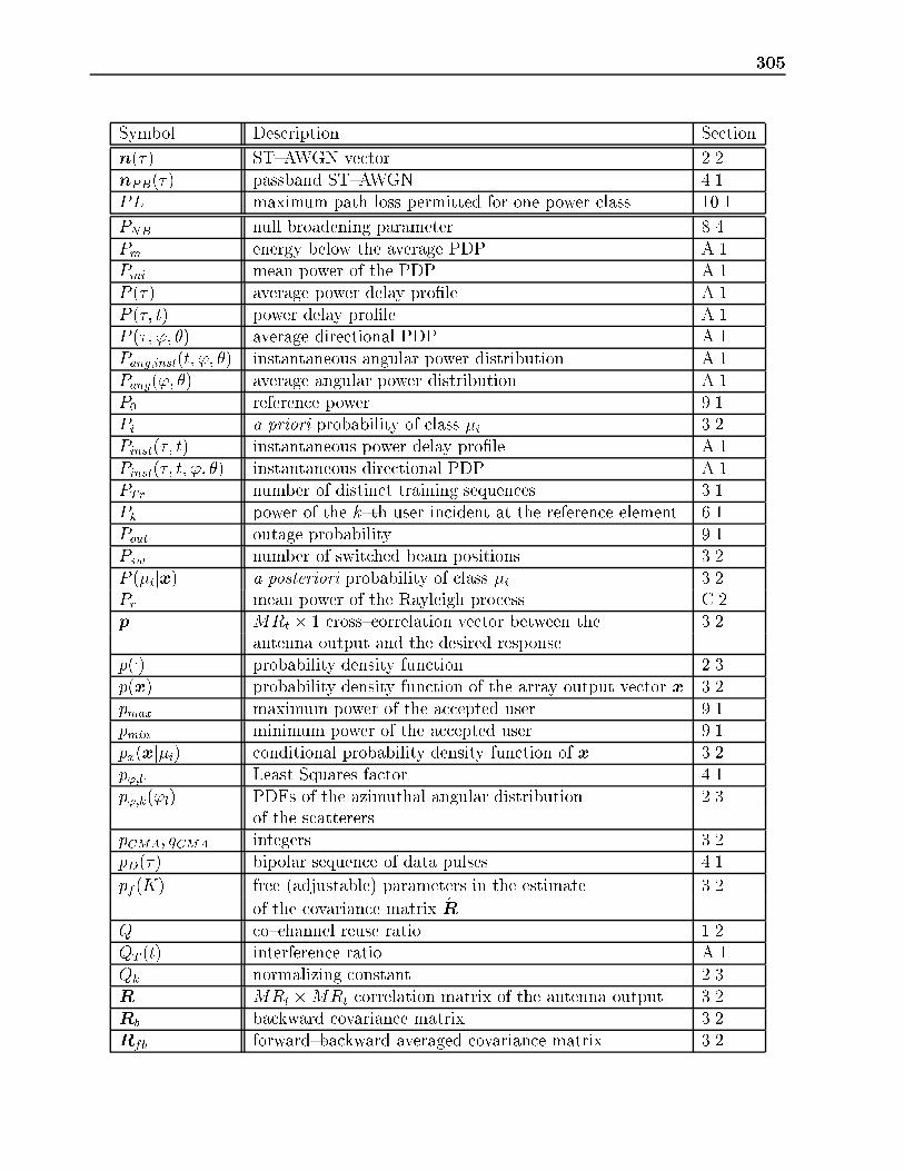
305
Symbol Description Section
n(�) ST{AWGN vector 2.2nPB(�) passband ST{AWGN 4.1PL maximum path loss permitted for one power class 10.1
PNB null broadening parameter 8.4Pm energy below the average PDP A.1Pmi mean power of the PDP A.1P (�) average power delay pro�le A.1P (�; t) power delay pro�le A.1P (�; '; �) average directional PDP A.1Pang;inst(t; '; �) instantaneous angular power distribution A.1Pang('; �) average angular power distribution A.1P0 reference power 9.1Pi a priori probability of class �i 3.2Pinst(�; t) instantaneous power delay pro�le A.1Pinst(�; t; '; �) instantaneous directional PDP A.1PTr number of distinct training sequences 3.1Pk power of the k{th user incident at the reference element 6.1Pout outage probability 9.1Psw number of switched beam positions 3.2P (�ijx) a posteriori probability of class �i 3.2Pr mean power of the Rayleigh process C.2p MRt � 1 cross{correlation vector between the 3.2
antenna output and the desired responsep(:) probability density function 2.3p(x) probability density function of the array output vector x 3.2pmax maximum power of the accepted user 9.1pmin minimum power of the accepted user 9.1px(xj�i) conditional probability density function of x 3.2p';l1 Least Squares factor 4.1p';k('l) PDFs of the azimuthal angular distribution 2.3
of the scattererspCMA; qCMA integers 3.2pD(�) bipolar sequence of data pulses 4.1
pf(K) free (adjustable) parameters in the estimate 3.2
of the covariance matrix RQ co{channel reuse ratio 1.2QT (t) interference ratio A.1Qk normalizing constant 2.3R MRt �MRt correlation matrix of the antenna output 3.2Rb backward covariance matrix 3.2Rfb forward{backward averaged covariance matrix 3.2

306 Frequently Used Symbols | Alphabetically Ordered
Symbol Description Section
Rn noise correlation matrix 3.2RTr block circulant matrix containing the 3.2
training sequences for the K usersRCS=SR matrix of correlation values 4.1RCS=SR;user new correlation matrix with L� 1 rows 4.1R radius of the scatterer circle 2.3Rf cell radius 1.2Rt number of temporal stages 3.2R(�) periodic cross{correlation function 3.1
of two training sequencesr training sequence 3.2rk;lk steering vector for the lk{th propagation path 8.2
for the k{th userrr truncated version of the training sequence 3.2rCS=TR correlation vector 4.1r radius of the scatterer ring 2.3r1 inner cell radius 2.3r2 outer cell radius 2.3rMS distance between BS and MS 2.3rMS;0 distance for reference point 9.1rc+1; rc radii of power class c 10.1rd(i) exponential correlation model 2.3
r(M)l distance from the mobile to the l{th scatterer 2.1
r(l)m distance from the l{th scatterer to the m{th antenna element 2.1rln(gLOS)(�) ACF of ln(gLOS) 2.3rCS=SR;max maximum of RCS=SR 4.1rCS=SR;th threshold value 4.1S(s) lower triangular matrix 3.2SNR vector containing the SNR's 3.2SNIR matrix of SNIRs of the di�erent synchronization instants 4.1SNIRmax Maxima of the SNIR of the di�erent rows 4.1SNIRup matrix with SNIRs determined from the uplink 8.1
SNIRup mean values of the uplink SNIRs 8.1S length of the training sequences 3.1S(j!) spectrum of the transmitted signal s(�) 3.2SBB constant envelope of the signal 4.1St average delay spread A.1Se spectral e�ciency 9.1Sf number of duplex channels 9.1(S'; S�) average angular spread A.1

307
Symbol Description Section
SNIRmax maximum SNIR 4.1SNRlin SNR at one antenna element on a linear scale 5.1SNRs;lin sum SNR on a linear scale 5.1s(�) vector containing the transmitted signals from the mobile 2.2sl;i output signal form an SR algorithm belonging to 4.1
the l{th DOA and the i{th synchronization instantsl;T r;n training sequence of the l{th signal 4.1sBS from the BS transmitted sum signal vector 4.2sc;BS signal vector in passband 4.2sk;BS from the BS transmitted signal vector for the k{th user 4.2sBB(�) complex envelope 4.1sf number of channels allocated to one cell 9.1sinst(t) instantaneous delay spread A.1sign(:) signum{function 3.2sr;m(�) received signal at the m{th antenna 2.3sr amplitude of the resolved signal 3.2snr amplitude of the non{resolved signal 3.2sc(�) complex RF{signal 4.1(s'(t); s�(t)) instantaneous angular spread A.1T JSA time instants, where the local maxima of SNIR(n) occur 4.1T CS=TR time instants, where the local maxima of rCS=TR occur 4.1T bit (symbol) duration 3.1Tm average mean delay A.1TCS=SR(l1) optimum sampling instants for the l1{th row 4.1t absolute time 2.1U 1 left singular vectors spanning the signal subspace 3.2U 2 left singular vectors spanning the noise subspace 3.2u(d) signal canceller weight vector 3.2V 1 right singular vectors spanning the signal subspace 3.2V 2 right singular vectors spanning the noise subspace 3.2V number of DOAs within a predetermined 6.1
angular region �'DOA~vMS velocity vector of the MS 2.1W estimated weighting matrix 3.2W set of array weight vectors for switched beam 3.2W down downlink array weight matrix 8.3Wq(t) delay window A.1w(n) array weight vector at the time instant � = nT 3.1wd;k downlink weight vector for the k{th user 8.1wr weight vector of the r{th stage 3.2

308 Frequently Used Symbols | Alphabetically Ordered
Symbol Description Section
~w(n) extended weight vector 3.2w(RBF )(n) coe�cient vector for the output layer 3.2wBd(n) d{th coe�cient of the feedback �lter 3.2w(x) complex probability function 2.3wRoom room width 2.4
wStreet street width 2.4X i one of I possible data sequences 4.1XT1&I1 matrix containing the tail and information 4.1
data of the �rst part of the burstXTr matrix containing the training sequence 4.1XI2&T2 matrix containing the information and tail data 4.1
of the second part of the burstx output signal vector of the BS antenna array 2.2x(b)(d) backward array data vector 3.2xm;sum sum data vector 3.2~x(n) extended data vector 3.2xBB;m(�) received signal in baseband 4.1xl;1m real part of gl;1m 2.3xrm;!1 real part of the signal srm;!1 at frequency !1 2.3xh(n) hypothesis symbol 3.2yRt(n) vector of the outputs of the Rt stages 3.2y(n) array output 3.1yr(n) output signal of the r{th stage at time instant � = nT 3.2yl;1m imaginary part of gl;1m 2.3yrm;!1 imaginary part of the signal srm;!1 at frequency !1 2.3Z direct{data matrix of the outputs of the hidden layer 3.2z(n) output vector of the hidden layer 3.2z(h) node output 3.2zmk mutual impedance 6.1zmm self impedance 6.1

309
Symbol Description Section
� power attenuation exponent 2.1�CMA input constant modulus 3.2
�(m)nl equivalent phase shift 2.3
� mean SNR C.2�i; i = 1; 2; 3 mean SNRs for GMSK (BtT = 0:3) C.2 instantaneous SNR C.2� angular width of the scatterer scenario as seen frm the BS 2.3�lm di�erence in pathlength between the scatterer 2.3
and two antenna elements�'s separation between the local scatterers 2.3
and the distant scatterers��k phase angle di�erence 4.1�� phase di�erence 2.3�'SB angular spacing of two consecutive beams 3.2�' angle between two co{channel users 5.2�'DOA angular width of the clustering region 6.1�'max�null distance between the maximum and the �rst null 5.0
of a broadside antenna pattern
�CIR di�erence of the mean CIR 9.1�CIR5% di�erence of the CIR at the 5%{level of Pout 9.1�(:) Dirac's delta pulse 2.1�RLS small positive constant 3.2"LS cost function for LS 3.2"RLS cost function for RLS 3.2�k(n) state of a single{user single{channel MLSE 3.2�ges overall spatial separability F�k1;k spatial separability of the two signals with index k1 and k F�; factorization matrices 3.2
�# factorization matrix � without the last row 3.2
�" factorization matrix � without the �rst row 3.2�k(n) superstate for the multiple{user vectorchannel MLSE 3.2� elevation angle 2.1�3dB 3dB beamwidth of the antenna pattern in elevation 2.2�('l � 'k) indicator function for the existence of wanted DOAs 3.1� inverse of the cross{correlation matrix 3.2� wavelength 2.1�d wavelength at the downlink frequency 8.3� step size parameter of the LMS algorithm 3.2�li elements of S(s) 3.2� forgetting factor 3.2

310 Frequently Used Symbols | Alphabetically Ordered
Symbol Description Section
�m m{th eigenvalue of R 3.2�env envelope correlation coe�cient 2.3~�xx real part of the correlation coe�cient 2.3~�xy imaginary part of the correlation coe�cient 2.3~�xx;�! frequency correlation coe�cient of 2.3
the real part of the signal~�xy;�! frequency correlation coe�cient of the 2.3
imaginary part of the signal�r;�! sum (frequency) correlation coe�cient 2.3�RBF width of f(:) 3.2� diagonal matrix containing the ordered eigenvalues of R 3.2�1 diagonal matrix containing the M ordered singular values of H 3.2�s
1 diagonal matrix containing the estimates 3.2of the eigenvalues
�2 noise power per antenna element 3.1�LOS standard deviation of the LOS signal amplitude 2.3�PC standard deviation of the power control error 9.2�r shape parameter 2.3�2s sum power of the paths 2.3�� standard deviation of the spread{out DOAs 2.3�' standard deviation of the pointing error 9.2� delay time 2.1�m(t) instantaneous mean delay A.1�o timing o�set 3.2
�(m)nl delay of the nl{th signal arriving at element m 2.3�2 delay of the second wavefront R 3.2� Power range in a cell�0 initial phase 4.1�0;BS starting phase of the local oscillator in the BS 4.2
�k phase angle 4.1�mod(�) excess phase 4.1' azimuthal angle 2.1'coverage angular section to be covered by the antenna 3.2'l;BS azimuthal angle under which the l{th scatterer 2.1
is seen from the BS'l;MS azimuthal angle under which the l{th scatterer 2.1
is seen from the MS'min minimum distance between the incident signals of two users 5.0'vMS
angle of the velocity vector of the MS 2.1'3dB 3dB beamwidth of the antenna pattern in azimuth 2.2�i; i = 1; 2 phase of the impulse response of the i{th user D

311
Symbol Description Section
('(t); �(t)) instantaneous mean direction of arrival A.1
(�;�) average mean direction of arrival A.1� continuous valued space variable 2.3
(�)m K � 1 state vector 3.2
of the sensor element m at time � phase shift 3.1!0 radian center frequency 2.3!do downlink angular frequency 4.2!m angular frequency shift 4.1

312 Frequently Used Symbols | Alphabetically Ordered

Index
AAir interface . . . . . . . . . . . . . . . . . . . . . . . . . . . iiiAlgorithms . . . . . . . . . . . . . . . . . . . . . . . . . . . . 45
categorization . . . . . . . . . . . . . . . . . . . . . . 50comparison . . . . . . . . . 113, 114, 131, 153computational complexity . . . . . . . . . . 92convergence speed . . . . . . . . . . . . . . 61{62in uence of angular separation . . . 113,
118, 131, 135, 137in uence of angular spread . . . 113, 122in uence of the air interface protocol45in uence of the channel . . . . . . . . . . . . 45linear . . . . . . . . . . . . . . . . . . . . . . . . . . . 50{79mobile communications . . . . . . . . . . . . 45modi�ed processing schemes . . . . 62{68nonlinear . . . . . . . . . . . . . . . . . . . 50, 79{91oversampling . . . . . . . . . . . . . . . . . . . 66{67performance for 4QAM . . . . . . . . . . . 150performance for GMSK . . . . . . . . . . . 131priciple . . . . . . . . . . . . . . . . . . . . . . . . . . . . 47signal reconstruction . . . . . . . . . . . 67{68SR . . . . . . . . . . . . . . . . . . . . . . . . . . . . . 70{79system requirements . . . . . . . . . . . . . . . 45TR . . . . . . . . . . . . . . . . . . . . . . . . . . . . . 50{70blind. . . . . . . . . . . . . . . . . . . . . .56, 68{69pros and cons . . . . . . . . . . . . . . . . . . . . 69training sequence . . . . . . . . . . . . . 56{68
weight control . . . . . . . . . . . . . . . . . . . . . .49Angular spread. . . . . . . . . . . . . . . . . . . . .20, 29
CDF . . . . . . . . . . . . . . . . . . . . . . . . . . . . . . . 23Antenna . . . . . . . . . . . . . . . . . . . . . . . . . . . . . . 113
1D{ULA . . . . . . . . . . . . . . . . . . . . . . . . . . . 47adaptive, operating principle . . . . . . . 49Bayesian . . . . . . . . . . . . . . . . . . . 81{83, 128broad nulls . . . . . . . . . . . . . . . . . . . . . . . 195BS . . . . . . . . . . . . . . . . . . . . . . . . . . . . . . . . . . 7BS, horizontal linear . . . . . . . . . . . . . . . . 8DFA. . . . . . . . . . . . . . . . . . . . . . . 80{81, 128elements . . . . . . . . . . . . . . . . . . . . . . . . . . . . 7
front to back ratio . . . . . . . . . . . . . . . . 226linear processing . . . . . . . . . . . . . . . . . . 128MLSE . . . . . . . . . . . . . . . . . . . . . 84{91, 128MS . . . . . . . . . . . . . . . . . . . . . . . . . . . . . . . . . 7MS, diversity . . . . . . . . . . . . . . . . . . . . . 239mutual coupling . 48, 77, 131, 137, 139nonlinear type . . . . . . . . . . . . . . . . . . . . 128null depth . . . . . . . . . . . . . . . . . . . . . . . . 226number of elements . . . . . . . . . . . . . . . 227omnidirectional . . . . . . . . . . . . . . . . . . . 209output vector . . . . . . . . . . . . . . . . . . . . . . 47pseudo{planar . . . . . . . . . . . . . 8, 153, 155sector . . . . . . . . . . . . . . . . . . . . . . . . . . 8, 209smart . . . . . . . . . . . . . . . . . . . . . . . . . iii, 7, 8topology . . . . . . . . . . . . . . . . . . . . . . . . . . 153
Arrayadaptivenarrowband . . . . . . . . . . . . . . . . . . . . . 164wideband . . . . . . . . . . . . . . . . . . . . . . . . 52
circular . . . . . . . . . . . . . . . . . . . . . . 153, 167square . . . . . . . . . . . . . . . . . . . . . . . 153, 174steering matrix. . . . . . . . . . . . . . . . . . . . .47steering vector . . . . . . . . . . . . . . . . . . . . . 47triangular . . . . . . . . . . . . . . . . . . . . 153, 174
arrayadaptivenarrowband . . . . . . . . . . . . . . . . . . . . . . 52
ATDMA . . . . . . . . . . . . . . . . . . . . . . . . . . . . . . . iii
BBaseband DSP . . . . . . . . . . . . . . . . . . . . . . . . . . 5Basedband DSP. . . . . . . . . . . . . . . . . . . . . . . . .8Bayes
array . . . . . . . . . . . . . . . . . . . . . . . . . . . 81{83law . . . . . . . . . . . . . . . . . . . . . . . . . . . . . . . . 81
BCCH . . . . . . . . . . . . . . . . . . . . . . . . . . . 235, 240BER
GMSK. . . . . . . . . . . . . . . . . . . . . . . . . . . .271GMSK, AWGN . . . . . . . . . . . . . . . . . . . 271
313

314 Index
GMSK, at fading . . . . . . . . . . . . . . . . 273GMSK, MRC . . . . . . . . . . . . . . . . . . . . . 276GMSK, selection diversity. . . . . . . . .275MSK, AWGN. . . . . . . . . . . . . . . . . . . . . 271MSK, at fading . . . . . . . . . . . . . . . . . . 273MSK, MRC. . . . . . . . . . . . . . . . . . . . . . . 276MSK, selection diversity . . . . . . . . . . 275
Broad nulls . . . . . . . . . . . . . . . . . . . . . . . . . . . 195BS
signal processing . . . . . . . . . . . . . . . . . . . 47
CCalibration . . . . . . . . . . . . . . . . . . . . . . . . . . 7, 75Call setup . . . . . . . . . . . . . . . . . . . . . . . 235, 236
MOC . . . . . . . . . . . . . . . . . . . . . . . . . . . . . 236MTC . . . . . . . . . . . . . . . . . . . . . . . . . . . . . 236
Capacity. . . . . . . . . . . . . . . . . . . . . . . . . . . . i, 203increase . . . . . . . . . . . . . . . . . . . . . . . . . . . . . iiincrease by smart antennas. . . . . . . .219in uence of imperfections . . . . 217, 228
Channel . . . . . . . . . . . . . . . . . . . . . . . . . 101, 111LOS{components . . . . . . . . . . . . . . . . . . 35model, high{rank, OLOS. . . . . . . . . .145model, ray{tracing . . . . . . . . . . . . . . . . 155modeling . . . . . . . . . . . . . . . . . . . . . . . 11, 12modelshigh{rank . . . . . . . . . . . . . . . . 14, 15, 36low{rank . . . . . . . . . . . . . . . . . 14, 15, 17parameters . . . . . . . . . . . . . . . . . . . . . . . 38
models, high{rank . . . . . . . . . . . . . . . . 145models, low{rank . . . . . . . . . . . . . . . . . 142scatterer distribution . . . . . . . . . . . . . . .17scatterers, moving. . . . . . . . . . . . . . . . . .36simulation model . . . . . . . . . . . . . 113, 133ST{AWGN. . . . . . . . . . . . . . . . . . . .48, 113
Channnelmodel, high{rank . . . . . . . . . . . . . . . . . 145
CIRincrease by smart antennas. . . . . . . .212threshold . . . . . . . . . . . . . . . . . . . . . . . . . 227
Cluster size . . . . . . . . . . . . . . . . . . . . . . 4, 5, 204CMA . . . . . . . . . . . . . . . . . . . . . . . . . . . . . . . . . . 68Co{channel reuse ratio . . . . . . . . . . . . . . . . 204Combining
MRC . . . . . . . . . . . . . . . . . . . . . . . . 105, 152
DDCA. . . . . . . . . . . . . . . . . . . . . . . . . . . . . . . ii, 226Detection
di�erential . . . . . . . . . . . . . . . . . . . . . . . . 109DFA . . . . . . . . . . . . . . . . . . . . . . . . . . . . . . . 80{81DOA iv, 11, 17, 20, 29, 41, 45, 47, 49, 226,
232, 236, 241clustering . . . . . . . . . . . . . . . . . . . . . . . . . 132estimation . . . . . . . . . . . . . . . . . . . . . . . . . 70nominal . . . . . . . . . . . . . . . . . . . 26, 44, 131
Downlink . . . . . . . . . . . . . . . . . . . . 99, 109, 177algorithms . . . . . . . . . . . . . . . . . . . . . . . . 178linear . . . . . . . . . . . . . . . . . . . . . . 178, 181nonlinear . . . . . . . . . . . . . . . . . . . . . . . 180
antenna pattern . . . . . . . . . . . . . . . . . . . . 46beamforming . . . . . . . . . . . . . . . . . . 75, 186assumptions . . . . . . . . . . . . . . . . . . . . 181broad nulls. . . . . . . . . . . . . . . . . . . . . .195compensation of propagation delays189
data collection . . . . . . . . . . . . . . . . . . 182optimization criterion . . . . . . . . . . . 185pre{equalization of propagation de-lays . . . . . . . . . . . . . . . . . . . . . . . . . . 191,201
null broadening . . . . . . . . . . . . . . . . . . . 283performance analysis . . . . . . . . . . . . . . 192power control . . . . . . . . . . . . . . . . . . . . . 238
DRA . . . . . . . . . . . . . . . . . . . . . . . . . . . . . . . . . . . ii
EESPRIT . . . . . . . . . . . . . . . . . . . . . . . . . . . . . . . 72
unitary . . . . . . . . . . . . . . . . . . . . . . . . . . . . 75
FFading
correlation, frequency . . . . . . . . . . 31, 46correlation, space . . . . . . . . . . . . . . . . . . 25 at . . . . . . . . . . . . . . . . . . . . . . . . . . . . . . . . 15frequency{selective . . . . . . . . . . . . . . . . . 15
Fading, large{scale . . . . . . . . . . . . . . . . . . . . . 14Fading, small{scale . . . . . . . . . . . . . . . . . . . . 14Frequency reuse factor . . . . . . . . . . . . . . . . 204
GGold sequences . . . . . . . . . . . . . . . . . . . . . . . . 47GSM. . . . . . . . . . . . . . . . . . . . . . i, 131, 141, 207

315
frame structure . . . . . . . . . . . . . . . . . . . . 46midamble . . . . . . . . . . . . . . . . . . . . . . . . . . 46power control . . . . . . . . . . . . . . . . . . . . . 219
HHalf{rate coder . . . . . . . . . . . . . . . . . . . . . . . . . iiHandover . . . . . . . . . . . . . . . . . . . . . . . . . . . . . . . 8Handovers . . . . . . . . . . . . . .217, 228, 235, 240HCS . . . . . . . . . . . . . . . . . . . . . . . . . . . . . . . . . . . . ii
IImpulse response
angle domain description. . . . . . . . . .260complex . . . . . . . . . . . . . . . . . . . . . . . . . . 257space domain description . . . . . . . . . 262statistical description . . . . . . . . . . . . . 257time domain description . . . . . . . . . . 257
Introduction . . . . . . . . . . . . . . . . . . . . . . . . . . . . 1
LLeast squares . . . . . . . . . . . . . . . . . . . . . . . . . . 57LMS. . . . . . . . . . . . . . . . . . . . . . . . . . . . . . . . . . . 61Local scatterer
model . . . . . . . . . . . . . . . . . . . . . . . . . . 11, 17
MMacrocells . . . . . . . . . . . . . . . . . . . . . . . . . . . . . 41Microcells. . . . . . . . . . . . . . . . . . . . . . . . . . . . . .41MLSE . . . . . . . . . . . . . . . . . . . . . . . . . . . . . . 84{91
channel estimation . . . . . . . . . . . . . . . . . 87impulse response estimation87{90, 277correlation . . . . . . . . . . . . . . . . . . . . . . . 90LS . . . . . . . . . . . . . . . . . . . . . . . . . . . . . . . 90
multiuser detection. . . . . . . . . . . . . . . . .86single{channel . . . . . . . . . . . . . . . . . . . . . 86trellisstate . . . . . . . . . . . . . . . . . . . . . . . . . . . . . 86superstate. . . . . . . . . . . . . . . . . . . . . . . .87
vector{channel. . . . . . . . . . . . . . . . . .84{91branch metric . . . . . . . . . . . . . . . . . . . . 86
NNetwork planning . . . . . . . . . . . . . . . . . . . . . 204Number of Signals
AIC. . . . . . . . . . . . . . . . . . . . . . . . . . . 72, 137MDL. . . . . . . . . . . . . . . . . . . . . . . . . .72, 137RoE . . . . . . . . . . . . . . . . . . . . . . . . . . . . . . . 73RoS . . . . . . . . . . . . . . . . . . . . . . . . . . . . . . 107
threshold . . . . . . . . . . . . . . . . . . . . . . . . . 107
Ooversampling . . . . . . . . . . . . . . . . . . . . . . . . . 103
PPicocells . . . . . . . . . . . . . . . . . . . . . . . . . . . . . . . 41Pointing errors . . . . . . . . . . . . . . . . . . . 217, 228Power class . . . . . . . . . . . . . . . . . 236, 237, 241Power control . . . . . . . . . . 219, 232, 235, 237
strategies . . . . . . . . . . . . . . . . . . . . 219, 228Power control errors . . . . . . . . . . . . . 217, 228
RReceiver . . . . . . . . . . . . . . . . . . . . . . . . . . . . . . 114
BS . . . . . . . . . . . . . . . . . . . . . . . . . . . . . 8, 101MS . . . . . . . . . . . . . . . . . . . . . . . . . . . . . . . 111
RF hardware. . . . . . . . . . . . . . . . . . . . . . . . . . . .7RLS . . . . . . . . . . . . . . . . . . . . . . . . . . . . . . . . . . . 58
fast . . . . . . . . . . . . . . . . . . . . . . . . . . . . . . . . 60
SSDMA . . . . . . . . . . . . . . . . . . . . . . . . . . iv, 3, 170
capacity . . . . . . . . . . . . . . . . . . . . . . . . 5, 220mean number of users . . . . . . . . . . . . .223
SFIR. . . . . . . . . . . . . . . . . . . . . . . . . . . . . . .3, 209capacity . . . . . . . . . . . . . . . . . . . . . . . . . . 205
SFU . . . . . . . . . . . . . . . . . . . . . . . . . . . . . . . . . . . . 3Signal canceller . . . . . . . . . . . . . . . . . . . . . 68{69Signal Processing . . . . . . . . . . . . . . . . . . . . . 102Simulation model . . . . . . . . . . . . . . . . . . . . . . 97Simulations
single user . . . . . . . . . . . . . . . . . . . . . . . . 133two users . . . . . . . . . . . . . . . . . . . . . . . . . 135
Space Division Multiple Access see SDMASpatial aliasing . . . . . . . . . . . . . . . . . . . . . . . . 48Spatial �lter . . . . . . . . . . . . . . . . . . . . . . . . . . . 49Spatial Filtering at the Uplink only. . . .see
SFUSpatial Filtering for Interference Reduction
see SFIRSpatial separability135, 142, 189, 192, 199,
281overall . . . . . . . . . . . . . . . . . . . . . . . . . . . . 281
Spatial smoothing. . . . . . . . . . . . . . . . . . . . . .71Spatio{Temporal Nyquist Criterion . 49{50Spectrum e�ciency. . . . . . . . . . . . . . . . .5, 205SQ{RLS. . . . . . . . . . . . . . . . . . . . . . . . . . . .59{60

316 Index
SR . . . . . . . . . . . . . . . . . . . . . . . . . . . . . . . . . . . 152array manifold . . . . . . . . . . . . . . . . . . . . . 75covariance matrix . . . . . . . . . . . . . . . . . . 71direct data matrix . . . . . . . . . . . . . . . . . 71forward{backward averaging . . . . . . . 74mutual coupling. . . . . . . . . . . . . . . . . . . .77SNIR/SR . . . . . . . . . . . . . . . . . . . . . . . . . 103weightmatrix . . . . . . . . . . . . . . . . . . . . . . . . . . . 74vector . . . . . . . . . . . . . . . . . . . . . . . . . . . .74
State{space model . . . . . . . . . . . . . . . . . . . . . 70STD . . . . . . . . . . . . . . . . . . . . . . . . . . . . . . . 63{64STD{SIMI . . . . . . . . . . . . . . . . . . . . . . . . . 64{66SVD . . . . . . . . . . . . . . . . . . . . . . . . . . . . . . . . . . . 72Switched beams. . . . . . . . . . . . . . . . . . . . . . . .54
optimum beam position . . . . . . . . . . . . 54Synchronization . . . . . . . . . 91, 102, 131, 156
algorithmslinear . . . . . . . . . . . . . . . . . . . . . . . . . . . . 91nonlinear. . . . . . . . . . . . . . . . . . . . . . . . .92
coarse . . . . . . . . . . . . . . . . . . . . . . . . . . . . 102CS/SR . . . . . . . . 103, 108, 149, 160, 163CS/TR . . . . . . . . 103, 105, 146, 156, 162�ne . . . . . . . . . . . . . . . . . . . . . . . . . . . . . . . 102JSA . . . . . . . . . . . . . . . . 103, 146, 156, 162SNIR/SR . . . . . . . . . . . . . . . . . . . . . . . . . 149SR. . . . . . . . . . . . . . . . . . . . . . . . . . . . . . . . . 92TR . . . . . . . . . . . . . . . . . . . . . . . . . . . . . . . . 91
System architecture . . . . . . . . . . . . . . . . . . . . 97change . . . . . . . . . . . . . . . . . . . . . . . . . . . . . . 7
TTraining sequences . . . . . . . . . . . . . . . . . . . . 269Transmitter
BS. . . . . . . . . . . . . . . . . . . . . . . . . . . . . . . .109MS . . . . . . . . . . . . . . . . . . . . . . . . . . . . . . . . 99
Trunking e�ciency . . . . . . . . . . . . . . . . . 5, 209
UUplink . . . . . . . . . . . . . . . . . . . . . . . . . . . . . . . . . 99
WWiener �lter
spatial . . . . . . . . . . . . . . . . . . . . . . . . . . . . . 56spatio{temporal . . . . . . . . . . . . . . . . 56{57

Curriculum Vitae
Personal:Josef Franz FUHLDate of birth: 05. February 1968Place of birth: Schwarzenbach, Austria
Nationality: �OsterreichCivil status: SingleAddress: A{2803 Schwarzenbach, Eggenbuch 17
Education:1974{1978 Volksschule (primary school)
at Schwarzenbach (Lower Austria)1978{1982 Hauptschule at Wiesmath (Lower Austria)1982{1987 H�ohere Technische Lehr{ und Versuchsanstalt
Wiener Neustadt ((Lower Austria)1987 Matura (high school diploma)1988{1993 Studies of Electrical Engineering
at the Fakult�at f�ur Elektrotechnik,Technische Universit�at Wien
1993 Degree of Diplom{Ingenieur1989{1994 Studies of Logics at the
Technisch{Naturwissenschaftliche Fakult�atUniversit�at Wien
1994 Degree of Magister rer. nat.1993{1997 Doctoral Studies at the Fakult�at f�ur Elektrotechnik,
Technische Universit�at Wien
Professional Experience:1984{1993 Summer jobs1993{1997 Research Assistant (Vertragsassistent) at the
Institut f�ur Nachrichtentechnik und Hochfrequenztechnik,Technische Universit�at Wien
Miscellanous:1987{1988 Military service, current position: �rst lieutenant
317


![Grid Generation Methods. 2nd Ed. - [Liseikin]](https://img.dokumen.tips/doc/110x75/56d6c07e1a28ab30169a9d83/grid-generation-methods-2nd-ed-liseikin.jpg)