Embed Size (px)
Citation preview

SMALL FLUCTUATIONS AT•THE UNSTABLE
STEADY STATE
by
Marc Mangel
B.S., Univ e r s i t y of I l l i n o i s , 1971
M.S., Un i v e r s i t y of I l l i n o i s , 1972
A THESIS SUBMITTED IN PARTIAL FULFILLMENT OF
THE REQUIREMENTS FOR THE DEGREE OF
i n the I n s t i t u t e of Applied Mathematics
We accept t h i s thesis as conforming to the
required standard
DOCTOR OF PHILOSOPHY
and
S t a t i s t i c s
THE UNIVERSITY OF BRITISH COLUMBIA
November, 1977
Marc Mangel, 1977

I n p r e s e n t i n g t h i s t h e s i s i n p a r t i a l f u l f i l m e n t o f t h e r e q u i r e m e n t s f o r
a n a d v a n c e d d e g r e e a t t h e U n i v e r s i t y o f B r i t i s h C o l u m b i a , I a g r e e t h a t
t h e L i b r a r y s h a l l m a k e i t f r e e l y a v a i l a b l e f o r r e f e r e n c e a n d s t u d y .
I f u r t h e r a g r e e t h a t p e r m i s s i o n f o r e x t e n s i v e c o p y i n g o f t h i s t h e s i s
f o r s c h o l a r l y p u r p o s e s may b e g r a n t e d b y t h e H e a d o f my D e p a r t m e n t o r
b y h i s r e p r e s e n t a t i v e s . I t i s u n d e r s t o o d t h a t c o p y i n g o r p u b l i c a t i o n
o f t h i s t h e s i s f o r f i n a n c i a l g a i n s h a l l n o t b e a l l o w e d w i t h o u t my
w r i t t e n p e rm i s s i o n .
D e p a r t m e n t
T h e U n i v e r s i t y o f B r i t i s h C o l u m b i a 2075 Wesbrook P l a c e V a n c o u v e r , Canada V6T 1W5
Small F luc tuat ions at the Unstable Steady State
Abstract
The e f fec t s of small random f l u c t u a t i o n s on d e t e r m i n i s t i c
systems are s tud ied . The d e t e r m i n i s t i c systems of i n t e r e s t have
m u l t i p l e steady s ta te s . As parameters v a r y , two or three of the
steady states coalesce . This work i s concerned with the long
time behavior of the system, when the system s t a r t s near an
unstable steady s ta te . The d e t e r m i n i s t i c s eparatr ix i s sur
rounded by a tube that contains up to two stable steady s ta te s .
The quant i ty of bas ic i n t e r e s t i s the p r o b a b i l i t y of f i r s t ex i t
from the tube through a s p e c i f i e d boundary, condit ioned on i n i t i a l
p o s i t i o n . In the d i f f u s i o n approximation t h i s p r o b a b i l i t y s a t i s f i e s
a backward d i f f u s i o n equation. Formal asymptotic so lu t ions of the
backward equation are constructed . The so lut ions are obtained by
a general ized "ray method" and are given i n terms of var ious
incomplete s p e c i a l func t ions . As an example, the e f fec t s of
f l u c t u a t i o n s on a substrate i n h i b i t e d r e a c t i o n i n an open ves se l
are analyzed. The theory i s compared with exact s o l u t i o n s , for
a one dimensional model; and Monte Carlo experiments, for a two
dimensional model.

i i i
Table of Contents
Section T i t l e Pages
Introduction and Summary of Results 1
Chapter 1 Stochastic Macrovariables with Coalescing Steady States . . . . 10
1 Fluctuations and Systems with M u l t i p l e Steady States 10
2 Spontaneous Generation of O p t i c a l A c t i v i t y : The Importance of Fluctuations at the Unstable Steady State . . . . 15
3 B i r t h and Death Approach to Chemical K i n e t i c s . . . . 19 4 Stochastic K i n e t i c Equations, Backward
Equation and F i r s t E x i t Problem 22 5 Three Canonical Integrals 27
5.1 Normal Case: The Error Integral 28 5.2 Marginal Case: The A i r y Integral 30 5.3 C r i t i c a l Case: The Pearcey Integral 32
Chapter 2 Asymptotic Solution of the F i r s t E x i t Problem i n the Normal Case 35
6 Normal Type Dynamical Systems 35 7 The Asymptotic Solution 36 8 Determination of IJJ and g^: Contours of
P r o b a b i l i t y 37 8.1 Determination of iKx) Q 37 8.2 Determination of z_, z^ and g 40 8.3 Contours of P r o b a b i l i t y 42
9 Completion of the F i r s t Term 42
Chapter 3 Asymptotic Solution of the F i r s t E x i t Problem i n the Marginal Case 44
10 Marginal Type Dynamical Systems 44 11 The Asymptotic Solution 46
11.1 Breakdown of the Error Approximation 46 11.2 Uniform Solution i n Terms of the A i r y Integral . 46
12 Evaluation of the parameter a~ 48 0
13 Determination of if and g : Contours of P r o b a b i l i t y 50 14 Completion of the F i r s t Term 51

Chapter 4 Asymptotic Solution of the First Exit Problem in the C r i t i c a l Case 53
15 C r i t i c a l Type Dynamical Systems 53 16 The Asymptotic Solution 55
16.1 Breakdown of Solutions using the Airy Integral . . 55 16.2 Uniform Solution in terms of the Pearcey Integral . 56
17 Determination of the Parameters 58 18 Determination of and g^: Contours of Probability. 59 19 Completion of the First Term 60 20 Two Complex Steady States . . . 62
Chapter 5 Fluctuation Effects on Substrate Inhibited Reactions • 64
21 Multiple Steady States in an Enzyme Reaction 64 21.1 Deterministic Kinetic Equations 64 21.2 Stochastic Model 67
22 Exact and Asymptotic Solutions 71 23 Comparison of the theory with Monte Carlo Experiments • 81
Bibliography 96
Appendices 101
A Solution of the I n i t i a l Value Problem for h^ 101
B Regularity of Higher Order Terms in the Expansion . . . 104
C Asymptotic Solution of the Expected Time Equation . . . 107
D Regularity at the Marginal Bifurcation 113
E Regularity at the C r i t i c a l Bifurcation 118
F Existence of Solutions of the General Eikonal Equation.,. 123

•,v
L i s t of Tables
Number T i t l e Page
I Exact and Asymptotic Solut ions i n the Normal Case . . 74
II Exact and Asymptotic Solut ions i n the Marginal Case • 75
I I I Exact and Asymptotic Solut ions i n the C r i t i c a l Case • 77
IV Exact and Asymptotic Solut ions i n the C r i t i c a l B i f u r c a t i o n 78
V Exact and Asymptotic Solut ions i n the Case of Two Complex Steady States 80
VI Comparison of the theory and experiment i n the Normal Case 83
VII Comparison of the theory and experiment i n the Marginal Case 86
V I I I Comparison of the theory and experiment i n the Marginal B i f u r c a t i o n 89
IX Comparison of the theory and experiment i n the C r i t i c a l Case 92
X Comparison of the theory and experiment i n the C r i t i c a l B i f u r c a t i o n 95

List of Figures
Number T i t l e Page
1 Normal Case 4
2 Marginal Case and Bifurcation 6
3 C r i t i c a l Case and Bifurcation 8
4 The First Exit Problem 14
5 Binaphthyl Model 18
6 Normal Type Dynamical System 35
7 Marginal Type Dynamical System • • • • 45
8 C r i t i c a l Type Dynamical System 54
9 Deterministic Phase Portrait and First Exit Boundaries in the Normal Case 82
10 Deterministic Phase Portrait and First Exit Boundaries in the Marginal Case 85
11 Deterministic Phase Portrait and First Exit Boundaries in the Marginal Bifurcation • • . . . . 88
12 Deterministic Phase Portrait and First Exit Boundaries in the C r i t i c a l Case 91
13 Deterministic Phase Portrait and First Exit Boundaries in the C r i t i c a l Bifurcation 94

Acknowledgements
I have been very fortunate to work with Professor Donald Ludwig,
whose knowledge, advice and encouragement were a great help to me.
Professor N e i l F e n i c h e l helped me understand the dynamical systems
studied i n t h i s work. For other use fu l d i s c u s s i o n s , I thank Professors
Robert Burgess (deceased), Robert Snider and Mr. Davis Cope.
This thes i s i s dedicated to Susan Mangel.

1
Introduct ion and Summary of Results
In t h i s sec t ion we formulate the problem of small f l u c t u a t i o n s
at the unstable steady s ta te . Examples of n a t u r a l systems which f i t
in to t h i s framework are g iven . F i n a l l y , we summarize the r e s u l t s
obtained i n the res t of the work. This sec t ion can be read independent
of the remaining sec t ions .
The evo lut ion of n a t u r a l systems i s often described by a
d e t e r m i n i s t i c d i f f e r e n t i a l equation:
x 1 = b 1 ( x , n , 6 ) x 1 ( 0 ) = x^ i = l , . . . , n . (1)
In equation (1) , n and 6 are parameters. A steady s tate i s
character ized by b 1 ( x , n , 6 ) = 0, i = l , . . . , n . I f b(x,n>5) i s
non l inear , the system may possess m u l t i p l e steady s ta tes . As the
parameters n and <5 v a r y , i t i s pos s ib l e that the steady states
coalesce and a n n i h i l a t e each o ther , or exchange s t a b i l i t y .
Equation (1) provides only an approximate d e s c r i p t i o n of the
evo lut ion of the system. In p a r t i c u l a r , i t ignores f l u c t u a t i o n s that
are inherent to a l l n a t u r a l systems. I f the system has m u l t i p l e
s table steady states (¥^,7^), f l u c t u a t i o n s may d r i v e the system
against the d e t e r m i n i s t i c flow so that ^Q^2^ * S r e a c n e d from an
i n i t i a l point which d e t e r m i n i s t i c a l l y i s a t t rac ted to V^O^Q) • In
t h i s case, the quant i ty of bas ic i n t e r e s t i s the p r o b a b i l i t y of a
s p e c i f i e d outcome, condit ioned on the i n i t i a l data . In t h i s work,
the behavior of the c o n d i t i o n a l p r o b a b i l i t y i s determined by so lv ing
the d i f f u s i o n equation that i t s a t i s f i e s , for the case of noise of

2
small i n t e n s i t y .
Many p h y s i c a l , chemical and b i o l o g i c a l systems f i t in to the
framework of f l u c t u a t i o n s superposed on a d e t e r m i n i s t i c d i f f e r e n t i a l
equat ion. Examples are : 1) L a s e r s , i n which f l u c t u a t i o n s are caused
by the quantum nature of r a d i a t i o n (Graham, 1974). 2) Tunnel diode
c i r c u i t s may e x h i b i t m u l t i p l e steady s ta tes . F luc tuat ions are caused
by the random motion of e lec trons (Landauer and Woo, 1972) . 3) The
mean f i e l d ferromagnet e x h i b i t s mul t ip l e steady states below the
c r i t i c a l temperature ( G r i f f i t h s et . a L , 1 9 6 7 , Go lds te in and S c u l l y ,
1973). 4) I somerizat ion , a u t o c a t a l y t i c , chain and substrate i n h i b i t e d
reac t ions i n open vesse l s may exh ib i t m u l t i p l e steady states ( P e r l -
mutter, 1972; Higg ins , 1967). F luc tuat ions are caused by the random
motion of the molecules , which may lead to a b i r t h and death
d e s c r i p t i o n of the r e a c t i o n process . 5) Membranes may e x h i b i t s tates
of high and low c o n d u c t i v i t y , separated by a threshold (e .g . Lecar and
Nossal,• 1971a,b ) . 6) The equations used i n t h e o r e t i c a l ecology may
e x h i b i t m u l t i p l e steady states (Bazekin, 1975). F luc tuat ions are
caused by the elementary b i r t h and death processes . The theory
developed i n t h i s work i s a p p l i c a b l e to a l l of the above systems.
As examples, we discuss a u t o c a t a l y t i c react ions ( § 2 ) and substrate
i n h i b i t e d react ions ( § 2 1 ) . The d i s c u s s i o n uses chemical terminology,
but the r e s u l t s are equal ly a p p l i c a b l e to physics and b io logy .
This work i s concerned with the e f fec t s of f l u c t u a t i o n s on
systems i n i t i a l l y i n the v i c i n i t y of an unstable steady s ta te . We
assume that the unstable steady s tate i s a saddle p o i n t , so that a
d e t e r m i n i s t i c s eparatr ix e x i s t s . The separatr ix d iv ides the phase
3
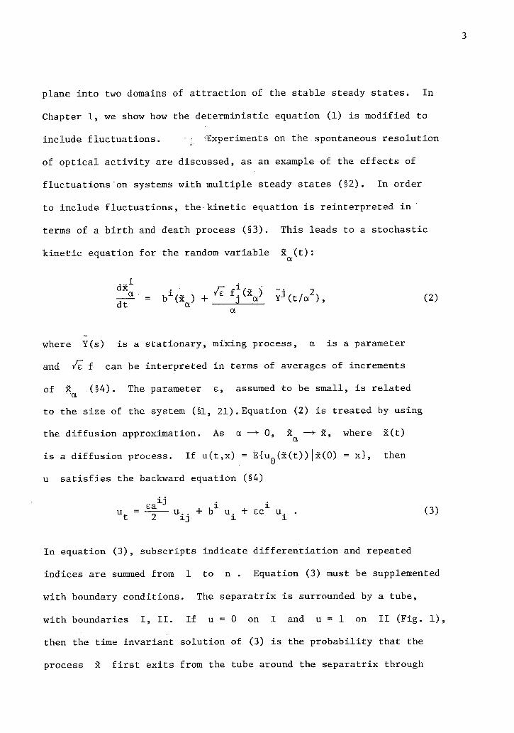
plane into two domains of attraction of the stable steady states. In
Chapter 1, we show how the deterministic equation (1) is modified to
include fluctuations. -;. Experiments on the spontaneous resolution
of optical activity are discussed, as an example of the effects of
fluctuations on systems with multiple steady states (§2). In order
to include fluctuations, the kinetic equation i s reinterpreted in
terms of a birth and death process (§3). This leads to a stochastic
kinetic equation for the random variable x^(t): a
dx 1
a • , l / ~ N . f .(%• ) / 2, ~ b (x ) + 2 a Y J(t/a ), (2) dt v a
a
where Y(s) is a stationary, mixing process, a is a parameter
and /e f can be interpreted in terms of averages of increments
of x^ (§4). The parameter e, assumed to be small, is related
to the size of the system (§1, 21). Equation (2) is treated by using
the diffusion approximation. As a —> 0, x^ —+ x, where x(t)
is a diffusion process. If u(t,x) = E{u^(x(t))|x(0) = x}, then
u satisfies the backward equation (§4)
i j • i u = • — — u. . + b u. + ec u. . (3) t 2 xj I I
In equation (3), subscripts indicate differentiation and repeated
indices are summed from 1 to n . Equation (3) must be supplemented
with boundary conditions. The separatrix is surrounded by a tube,
with boundaries I, II. If u = 0 on I and u = 1 on II (Fig. 1),
then the time invariant solution of (3) is the probability that the
process x f i r s t exits from the tube around the separatrix through

4
boundary II, given that x(0) = x . Asymptotic solutions of (3) are
constructed. The method of solution is a generalization of the ray
method of Luneberg (1948) and Keller (1958). The ray method uses a
formal asymptotic technique to convert the second order boundary value
problem for u(x) to a f i r s t order i n i t i a l value problem for a
function ij>(x) • The f i r s t order problem can be treated by the method
of characteristics (§5).
The form of the asymptotic solution depends upon the deterministic
system (§5). In the normal case, the three steady states are well
separated and only the unstable steady state is contained by the
separatrix tube (Fig. 1).
Fig. 1 Normal Case

5
The asymptotic solution of the time invariant backward equation
i s :
u(x) = I E Y ( x)E ( | ( x ) / / D + ^ ^ ( x l E ' r t t x ) / ^ ) , (4) n=0
where E is the error function: E"(z) =--zE'(z). The functions
}Kx), g n(x) and h n(x) are to be determined (§7). The form of
(4) i s suggested by the asymptotic expansion of a simpler problem
( § 5 ) . The function ip(x) must satisfy
i a ± j
b\ - ^ - = 0 . (5)
By using Hamilton-Jacobi theory, we show that tp(x) is constant on /
the deterministic separatrix (§8). The derivatives of ip are cal
culated on the separatrix. Thus, in a vi c i n i t y of the separatrix
ip(x) can be calculated by a Taylor expansion. We show that g*"* is
a constant (§8). The value of g^ is chosen so that the boundary
conditions are satisfied. Once ip and g^ are known, the leading
part of the asymptotic solution,
u(x) ^ g°EO(x)/v^) + 0(/e~) (6)
can be used to generate contours of equal probability in the plane
(§8.3). The function h^(x) can be evaluated everywhere in the
phase plane (§9 and Appendix A). Higher order terms are treated in
an analogous fashion (Appendix B).
In the marginal case (§10), two steady states are contained
by the separatrix tube (Fig. 2a). As one parameter varies, the two

(a) (b)
Fig. 2 Marginal Case (a) and Bifurcation (b)
steady states coalesce and annihilate each other. The detailed
properties of such a deterministic system are given in §10. The
uniform asymptotic solution of the time independent backward equation
is (§11)
u(x) = I en A 0 j , / £
1 / 3 , a/e 2 / 3)g n(x) (7)
. n+2/3.,,,, 1/3 , 2/3., n, . + e A' ( l p / e , a/e )h (x)
2 where A is the incomplete Airy integral: A"(z,B) = -(z -B)A',

and cx = 2, a vE • The form of (7) is suggested by the asymptotic is, ,
analysis of a simpler problem (§5) . The function iKx) and parameter
CIQ must be determined to satisfy:
i a ± j 2 •b i|>± - ^ (* -oQ) = 0 . (8)
Using Hamilton-Jacobi theory, we show that ip is constant on the
separatrix (§12). The parameter is determined by using the
method of characteristics (§12). The function i\i and constant g^
are evaluated as in the previous case (§13). Once ij/, and g^
are known, the leading part of the asymptotic expansion:
u(x) <b g°A(^(x)/ e1 / 3,a 0/ e- 2 / 3) + 0 ( e 2 / 3 > (9)
can be used to generate contours of equal probability (§13). The
function h^ can be calculated everywhere in the phase plane (§14
and Appendix A). Higher order terms are treated in an analogous
fashion (Appendix B).
In Appendix D, we show that a l l of the constructions are regular
at the marginal bifurcation. At the bifurcation point, of more
interest than u(x) is
T(x) = E{time for x(t) to hit ll|x(0) = x, x(t) hits II} (10)
In §4, we show that
i j T.. + b 1!. + ec^T. = -1 . (11) 2 xj i x
The asymptotic solution of (11) is constructed in Appendix C. The

solution involves a special function similar to A(z,a), but
satisfying an inhomogeneous differential equation.
In the c r i t i c a l case, three steady states are contained by the
separatrix tube (Fig.3). As n, <5 vary the steady states coalesce
into one stable steady state.
(a) (b)
Fig.3. C r i t i c a l Case (a) and C r i t i c a l Bifurcation (b)
The detailed properties of a c r i t i c a l type dynamical system are given
in §15. The asymptotic solution of the time independent backward
equation is
u(x) = I e g (x)P(i{j/e ,a/e ,g/e ) (12)
, ri+3/4 n, 1/4 , 1/2 0 . 3/4, + e h (x)P'(ip/e ,a/e ,3/e )

9
3 where P is the Pearcey integral: P"(z,a,8) = (z -az-g)P'(z,a,g),
a = y a, e " and 3 = 7 8 (§16). The function ip(x) and parameters u k k 01Q, 8Q must be determined so that
i 3 a ± j
b t j ; . + ( i j, J-a 0 i p-g 0) — ^ = 0 . (13)
The parameters a^, 8Q and functions IJJ, g^ are evaluated in a
manner analogous to the previous cases (§17, 1 8 ) . Once a^, 8Q, ip
and g^ are known, contours of equal probability can be generated
( § 1 8 ) . The function h^(x) can be evaluated everywhere in the plane
(§19 and Appendix A). Higher order terms are treated in an analogous
fashion (Appendix B). In Appendix E, we show that a l l constructions
are regular at the bifurcation point and determine power series for
dp,. BQ in terms of n » 6 . These power series are useful i f the
deterministic system has two complex steady states with small imaginary
part ( § 2 0 ) .
An application of the above theory is presented in the f i n a l
chapter. A model of Degn's experiments on NADH oxidation is presented
in §21.1. The stochastic version is derived in §21.2. By assuming
perfect control of one of the variables, the model becomes one dimensional.
The asymptotic theory can then be compared with an exact solution
( § 2 2 ) . The asymptotic results are accurate. The two dimensional
asymptotic theory is compared with Monte Carlo experiments in §23.

10
Chapter 1: Stochastic Macrovariables with Coalescing
Steady States
1. Fluctuations and Systems with Multiple Steady States
The classical method of describing the evolution of chemical
reactions i s by the use a' deterministic differential equation
x = b(x) x £ Rn . (1.1)
In (1.1), x is a macroscopic variable that represents concentrations
of reactants or products. The macrovariable
describes the average state of a large system and is obtained by
averaging over many independent subunits. The form of b(x) is
determined by the reaction mechanism.
Steady states are characterized by b(x) = 0 . If b(x) is
nonlinear, then the system may have multiple steady states. The
eigenvalues of B = (b 1, ) can be used to characterize the type of
steady state. If a l l eigenvalues have non zero real part, the steady
state i s of the normal type. Following Kubo et. a l . (1973) we dis
tinguish two kinds of non-normal steady states: 1) the marginal 2
type, in which the local dynamics are x ^ x ; 2) the c r i t i c a l type, 3
in which the local dynamics are x 'v x . A steady state i s stable
i f a l l eigenvalues have negative real part. Otherwise is is unstable.
The deterministic approach can be improved i f s t a t i s t i c a l fluctuations
are included. The concentrations, represented by a random variable
x(t), w i l l fluctuate for two reasons (Keizer, 1975). Fi r s t , due to

experimental limitations, i t is impossible to specify concentrations
exactly. Second, even i f the concentrations were known at some time
t, the exact concentrations at a later time t + At would not be
known unless a l l of the microscopic variables were known at time t .
The specification of a l l the microscopic variables i s , pregently, not
possible. With this, viewpoint, equation (1.1) describes the average
behavior of a large number of s t a t i s t i c a l variables. A more exact
description of the system would specify the volume V of the reaction
vessel and an integer valued random variable X(t) that represents
the number of molecules in V at time t . The mean of x(t) = X(t)/V
w i l l correspond to the deterministic concentration. The variance of
x(t) provides a measure of s t a t i s t i c a l fluctuations (McQuarrie, 1967).
In chemical systems the intensity of fluctuations is proportional
to 1/V (Keizer, 1975; Van Kampen, 1976). In macroscopic systems,
V is large so that the fluctuations are of small intensity. When
the fluctuations are of small intensity, equation (1.1) usually
provides an adequate description of the evolution of the system.
There are, however, exceptions, some of which have been studied. When
reactions occur in relatively small volumes (e.g. biological cells)
or involve small numbers of molecules, fluctuations can have a profound
effect on the evolution of the system (Delbruck, 1940; McQuarrie, 1967).
I n i t i a l fluctuations w i l l be amplified in autocatalytic or chain
reactions (Singer, 1940). In the sequel, we set e <* 1/V (see § 21).
Many authors have studied the effects of fluctuations on systems
in the v i c i n i t y of the stable steady state (Lax 1960, 1966; Nitzan et a l
1974). In .this work, we investigate the effects of fluctuations on
systems i n i t i a l l y in a v i c i n i t y of a kinetic saddle point. There are
a number of reasons for studying chemical systems in the v i c i n i t y of
an unstable steady state. In the f i r s t place, one would like to verify
that the unstable steady state exists (Chang and Schmitz, 1975). Due
to fluctuations, i t is not possible to observe the unstable steady
state. In later chapters, we w i l l show that the unstable steady state
has a certain probabilistic description. Secondly, in many reactions
the stable steady states represent ^ 0 or 100% completion of the
reaction. The most significant kinetic information is obtained from
rate data in a v i c i n i t y of the unstable steady state. Chang and
Schmitz (1975) point out that often i t is desirable to start a chemical
reactor near the unstable steady state, but that one stable steady
state is preferred. In this case, one wishes to estimate the pro
bability that the less desirable stable state is reached. The gating
mechanisms of nerve membranes involve reactions with multiple steady
states (Armstrong, 1975). The study of fluctuations at the unstable
steady state (threshold) may lead to information about conductivity
mechanisms (Lecar and Nossal, 1971a, b).
In practice, i t is very d i f f i c u l t to prepare a system in an
unstable steady state. However, many systems exhibit behavior in which
a stable steady state becomes unstable as a parameter is varied (Degn,
1968, Pincock et. a l . 1971, Lavenda, 1975). When a parameter a is
less than a c r i t i c a l value a^, the system has only one steady state,.
P, , which is stable. When a is increased, so that a > a , P.. 1 c 1
becomes unstable and two stable steady states P^, P^ are created.
We c a l l this the c r i t i c a l bifurcation. The mean-field ferromagnet

exhibits such behavior. Many chemical systems also exhibit the c r i t i c a l
bifurcation (§2, §21). A second type of bifurcation is possible as
a increases. The steady state P., remains stable when a > a 1 c
and two new steady states Q^, which is unstable, and QQ, which
is stable, appear. We c a l l this the marginal bifurcation. The
marginal bifurcation has not received adequate attention in the
chemical literature because there is a feeling among chemists and
physicists that one can not observe i t . In §22-23 we shall demon
strate that substrate inhibited reactions may exhibit the marginal
bifurcation.
If P^ i s unstable when a > a^, the system w i l l always leave
a neighborhood of P^ and approach P^ or P . Even i f the system
were i n i t i a l l y at P^, any minute fluctuation w i l l cause i t to leave
the neighborhood of P^ . In the vi c i n i t y of an unstable steady
state, fluctuations can never be ignored. According to the
deterministic theory, the separatrix (Fig. 4) S divides the phase
plane into two domains of attraction. A l l phase points i n i t i a l l y
on one side of S approach P^; phase points on the other side
approach • Points i n i t i a l l y on 5 approach the saddle point P l '
When a more exact, stochastic description i s used, the
deterministic picture must be modified. No phase points w i l l reach
P^ and remain there. Due to fluctuations, a l l phase points reach
a v i c i n i t y of PQ or . More importantly, phase points which
deterministically would approach P^ might approach P^ (and vice
versa). Namely, fluctuations may drive the system against the

d e t e r m i n i s t i c f l o w . I d e a l l y , one would l i k e to c a l c u l a t e t h e
p r o b a b i l i t y t h a t a s p e c i f i e d s t e a d y s t a t e i s reached f i r s t . T h i s
problem i s g e n e r a l l y too d i f f i c u l t t o s o l v e . I n s t e a d , we surround
the s e p a r a t r i x by a tube w i t h b o u n d a r i e s I , I I ( F i g . 4 ) .
We w i l l c a l c u l a t e the p r o b a b i l i t y , u ( x ) , t h a t t h e p r o c e s s x ( t ) f i r s t
e x i t s from t h i s tube through boundary I I , g i v e n t h a t x(0) = x .
In the d i f f u s i o n a p p r o x i m a t i o n , t h i s p r o b a b i l i t y s a t i s f i e s a d i f f u s i o n
e q u a t i o n . We s h a l l c o n s t r u c t f o r m a l a s y m p t o t i c s o l u t i o n s of the
d i f f u s i o n e q u a t i o n . Our t e c h n i q u e w i l l c o n v e r t the second o r d e r
boundary v a l u e problem f o r u to a f i r s t o r d e r i n i t i a l v a l u e problem
f o r a new f u n c t i o n . A l t h o u g h we w i l l g i v e an e x i s t e n c e p r o o f f o r
F i g . 4 . F i r s t E x i t Problem

15
ip(x) (Appendix F), we do not prove that our solution is asymptotic
to the true solution.
2. Spontaneous Generation of Optical Activity: The Importance of
Fluctuations at the Unstable Steady State
The experimental work of Pincock et. a l . (1971) provides an
example of a chemical system in which a stable steady state becomes
unstable as a parameter varies. The experiments also indicate the
importance of fluctuations in determining the evolution of a system
i n i t i a l l y in the v i c i n i t y of an unstable steady state.
1,1' Binaphthyl has enantiomers which are interconverted by a
bond rotation. At room temperature, the rotation i s sufficiently
slow so that a molecule is "fixed" in one conformation. Above 160°C,
the interconversion rate has a half l i f e of 0.5 seconds, so that a l l
mixtures are racemic above 160°C. The experiments involved heating
samples of binaphthyl above 160°C and then rapidly crystallizing
the melt. The optical activity of the resulting crystal was determined.
The distribution of specific rotation in 200 experiments was -218° to
206°, with mean 0.14°. The distribution of the data was similar to
the distribution of "heads" i f a f a i r coin were flipped 8 times. •
A;,complex nucleation process is involved in these experiments. The following
simple model illustrates the phenomenon of interest here. Assume that each
sample contains a large number of microfeglons, which act independently.
Above 160°C, the racemic statesis stable and a l l microregions are racemic.
Below 160°C, the two resolved states are stable. In each microregion,

"a f a i r coin i s f l i p p e d " to decide the f i n a l o p t i c a l a c t i v i t y
of the region. Although some samples remained i n a supercooled
racemic state f o r a few hours, no sample remained i n the racemic
state i n d e f i n i t e l y . The r e s o l u t i o n of o p t i c a l a c t i v i t y was completely
determined by random f l u c t u a t i o n s .
The p r o b a b i l i t y of achieving a given resolved state was modified
by the addi t i o n of c e r t a i n o p t i c a l l y a c t i v e substances. For example,
when 2.5 weight % D(-) mandelic acid was added to the. racemic mixture,
21 samples with negative r o t a t i o n and 7 samples with p o s i t i v e r o t a t i o n
were obtained. The p r o b a b i l i t y of observing such a r e s u l t with a
" f a i r c oin" i s .004. When the concentration of mandelic acid was
doubled, 27 (-) samples and 0 (+) samples were obtained. The —8
p r o b a b i l i t y of observing t h i s r e s u l t with a f a i r coin i s 1.5 x 10
Thus, the ad d i t i o n of mandelic acid at low concentrations (12-24
binaphthyl molecules/mandelic acid molecule) affected the evolution
of the system.
In order to understand these experiments, we consider the following 1 2
simple mathematical model. Let x , x denote the concentrations
of (+), (-) enantiomers r e s p e c t i v e l y . Following Frank (1953) we
assume that each enantiomer i s the c a t a l y s t for i t s own production
and the a n t i c a t a l y s t f o r the other enantiomer. Let R denote the
racemic melt, which i s treated as a constant source of molecules.
The reaction scheme i s :

X 1 + R 2X1
x 2
T K »" /A "V , „ } autocatalytic step
+ R i±2U 2X2 / 1 2 a
X + X -^-> 2R (2.1) X I + X 1 -^-> inert „2 , v2 1 X + X >• inert
The last two steps were added to insure that a l l concentrations remain
bounded. They might correspond to molecules which are no longer on
the surface and hence are inert to catalysis. The kinetic equations
(with R = 1) are
.1 1 1 2 1 2
x = (l+a)x - ax x - (x ) (2.2)
.2 2 1 2 2 2 x = (l+a)x - ax x - (x ) (2.3)
The rate parameter a is assumed to be a function of temperature such
that a > 1 i f T < 160°C and a < 1 i f T > 160°C .
When T > 160°C, a < 1, the only steady state is (1,1), which
is stable (Fig. 5a). When a > 1, T < 160°C, the racemic state is 1 2
unstable. Two stable steady states appear on the x and x axes (Fig. 5b). The racemic state in this special model is the entire
1 2
separatrix S: x = x . When a > 1, i f the sample is i n i t i a l l y
in the racemic state, any small fluctuation w i l l cause the sample, to
evolve towards one of the resolved states.
The experiments with mandelic acid can be explained using this
model. For example, point A in Fig. 5b might represent an experiment
in which 2.5% mandelic acid was added. An experiment starting at
point A is more likely to approach 0 than an experiment starting

18
(a) a < 1 (b) a > 1
Fig. 5. Binaphthyl Model
at 0 . The result of an experiment starting at point B w i l l
probably not be affected by fluctuations of small intensity.
In this model, the multiple steady states arise in a natural
fashion due to the nonlinearity of the kinetic equations.
Fluctuations can be included by treating the reactions (2.1) as a
birth and death process (§3).
The theory developed in Chapter 2 can be used to treat the
above model of the binaphthyl experiments when fluctuations are
included.
The model=in=this section i s , of course, an oversimplification of
the physical nucleation process. However, the model illustrates how
fluctuations may affect systems with multiple steady states.
19
3. Birth and Death Approach to Chemical Kinetics
The birth and death approach provides a method for giving a
st a t i s t i c a l interpretation to macroscopic chemical kinetics
(Bartholomay, 1957; McQuarrie, 1967). For the purposes of illustration,'
consider the following reactions which appear in the work of Harrison
(1974) and Glansdorff and Prigogine(1971):
k l
A + 2B 3B (3.1) k2
B -=-*• C (3.2)
Let k = k^[A], x = [B] and assume that [A] is a constant. The
kinetic equation for x is 2
x = kx - k^x. . (3.3)
Equation (3.3) has steady states x = 0 (stable) and x = k2/k =
(unstable). We assume that other reactions insure that x does ,not become
unbounded, but x^rnayCattain a•-sta'ble<-steady • state x , with x > x . . s s s u
If x(0) = XQ, the deterministic description of the reaction
is as follows. If XQ < x^, then x(t) —* 0 as t increases. If
x« = x , then x(t) = x for a l l t . If x_> x , then x(t) —»- x 0 u u 0 u s as t increases.
In the stochastic approach, reaction (3.1) is treated as a birth
of a molecule of B; reaction (3.2) is a death of a molecule of B .
Let X(t) be a random variable that represents the number of molecules
of B in the reaction vessel, of volume V, at time t . We assume
that the following transition probabilities exist:
Pr{X( t+At) - X ( t ) = l | x ( t ) = X} = aX 2 At + o ( A t ) (3.4)
Pr{X(t+At) - X(t) = -1 X(t) = X} = 3XAt + p^'At) (3.5)
Pr{all higher transitions} = o(At) . (3.6)
By using forward differences in equations (3.4 - 3.6), we are
making an implicit assumption about the stochastic process. Different
approaches (e.g. centered differences) are also possible. The choice
of forward differences agrees with McQuarrie (1967) and Bartholomay
(1957). The constants a, 3 are determined by requiring that
E(X(t)) satisfy the law of mass action (3.3).
Let AX = X(t+At) - X(t) . Using equations (3.3 - 3.6):
We require that (3.8) and (3.3) agree, when (3.8) is rewritten in
terms of the concentration variable x = X/NV, where N is Avogadro's
number and X = E(X) . Equation (3.8) becomes
E(AX|x(t) = X) = (aX2 - BX)At + o(At) (3.7)
We define
(3.8)
x = aNVx - Bx, (3.9)
which w i l l agree with (3.3) i f
a = k/NV and (3.10)
A measure of inherent fluctuations about the mean is provided
by the infinitesimal variance (Feller, 1971):
a(X) = lim j- E{(AX ) 2 | x(t) = X} . (3.11) At-K)
Using the transition probabilities (3.4 - 3.6), we find
a(X) = aX 2 + gX . (3.12)
In general, many different reaction mechanisms can produce the same
rate law. The stochastic approach provides a more accurate description
of the system, since the chemical mechanism figures prominently in
the calculation of b(X) and a(X) .
McQuarrie (1967) presents an extensive discussion in which mean
motion and fluctuation effects are compared. We note the following
points:
1) McQuarrie did not allow b(X) to vanish, i.e. that the
system has a steady state. At an unstable steady state, fluctuations
greatly influence the behavior of the system.
2) Experimental techniques are available for the direct measure
ment of fluctuation effects in chemical reactions (Feher and Weissman,
1973, Vereen and De Felice, 1974).
3) Experimentalists working with chemical reactors are concerned
with fluctuation effects (Chang and Schmitz, 1975). Chang and Schmitz
do not estimate the intensity of the fluctuations, but i t is clear
from their discussion that the fluctuations are of concern.

22
4. Stochastic Kinetic Equations, Backward Equation and First
Exit Problem
The macrovariable x(t) represents the average concentrations
of reactants at time t and evolves according to the kinetic
equation
x 1 = b 1(x) x 1(0) = xj i = 1,2 . (4.1)
According to the s t a t i s t i c a l theory of chemical kinetics, x(t) is
the mean value of a random variable x(t), which w i l l satisfy a
stochastic kinetic equation. It is not yet possible to derive the
stochastic kinetic equation from basic principles. Ideally, one
would start with the Liouville equation and reduce i t to a stochastic
kinetic equation. This reduction has been performed only on the
simplest system (Sinai, 1970). Instead, we shall use a Langevin
method (Lax, 1966) and add a stochastic term to the right hand side
of (4.1). The source of the stochastic term is the random motion
of the solvent and solute molecules, which occurs on a time scale
T, small compared to the macroscopic time scale t, on which
measurements are made.
The increments in T and t are related by a parameter a:
Ax = At • a 2, (4.2)
2
where a w i l l characterize the fast time scale. The random process
generated by the microscopic motions is assumed to be a mixing process
Y(T) . In most of the physical literature (e.g. Mori, 1965; Ma, 1976)
i t is assumed that

E[Y K( S)Y^(0).] = 6^(3) (4.3)
k£ where 6 (s) = 0 unless k = L and s = 0 . We shall not make
this assumption and define
Y E[Y k(s)Y £(0)]ds . (4.4) 0
In the case that (4.3) holds, Y(T) is the "white noise"
process. We assume that the stochastic variable x(t;a)
satisfies
dx X(t;a) . o.(x) ...
dt b^x) + JZ -1 Y J(t/a ) i = l , . . . , n . (4.5)
Langevin was the f i r s t to use a kinetic equation of the form (4.5)
(Lax, 1966). Such equations have been used in the last f i f t y years
by almost a l l physical scientists working in this f i e l d . The use of
(4.5) represents an approximate, somewhat ad hoc, way of treating
stochastic effects in macroscopic systems. Equation (4.5) is the
stochastic kinetic equation that w i l l be used in the rest of this
work.
The functions b 1(x) appearing in (4.5) are the same functions
appearing in the macroscopic equation (4.1). They determine the
average or macroscopic evolution of x(t) . For example, for the
model of binaphthyl experiments
1 1 1 2 1 2 b (x) = (l+a)x - ax x - (x ) (4.6a) 2 2 1 2 2 2
b (x) = (l+a)x - ax x - (x ) . (4.6b)

24
The function Y(s) is a zero mean process, satisfying the mixing
hypothesis of Papanicolaou and Kohler ( 1 9 7 4 ) . The f i e l d a j ( x ) i s assumed
to be known. It characterizes the x dependence of the fluctuations.
Since ( 4 . 5 ) is not derived from f i r s t principles, we need to provide
a prescription for the calculation of a(x) . In §21, we discuss
how a(x) can be calculated. We assume that x(0;a) = x^ remains
a deterministic condition.
As a —*- 0, x(t;a) converges to a diffusion process x(t)
(Papanicolaou and Kohler, 1 9 7 4 ) . Let u Q ( x ) D e integrable and
u(t,x) = E{u Q(x(t))|x(0) = x} . (4.7)
Then u(t,x) satisfies the backward equation
u^ = ——u_. + b u_. + ec u. (4.8)
where
*t 2 " i j " i " i
a l j(x) = a^(x)aJ(x)( Yk £ + Y ^ ) ( 4 . 8 a )
c i ( x ) = Y ^ ol - \ ( o b ( 4 . 8 b ) R 9x 3 J L
If Y(T) were white noise, the resulting diffusion equation
would be i j
u„ = u. . + b \ i . . ( 4 . 9 ) t 2 i j l
If a±2 is independent of x, then equations ( 4 . 8 ) and ( 4 . 9 ) are
identical. In §22, we present a numerical comparison of solutions
of equations ( 4 . 8 ) and ( 4 . 9 ) . Our results indicate that ( 4 . 9 ) is an

25
excellent approximation to (4.8) i f the boundaries are non-singular.
The fundamental equation derived above is (4.8) or i t s time
independent version
0 = u. . + bV + ecV . (4.10) 2 13 l x
Equation (4.10) must be supplemented by boundary conditions i f the
problem is to be properly posed. We surround the separatrix by a
tube with boundaries I, II . If u = 0 on I, u = 1 on II,
then u(x) is the probability that x(t) f i r s t exits from the tube
around the separatrix through boundary II . Let the boundaries be determined
by f I(x) = 0, fi;E(x)=.0.. Let HI(t)=0 i f fj(x(s))=0 for some s, 0<s<t and 1
otherwise. The u Q(x(t)) in (4.7) is 6 (f (x(t) ))iH^'(t) .
We distinguish three cases of increasing complexity.
1) The Normal Case : in which the separatrix tube contains
only the unstable steady state.
2) The Marginal Case.:'' in which the separatrix tube contains
the unstable steady state and one stable steady state. As one
parameter varies, the two steady states coalesce and annihilate each
other (the marginal bifurcation). After the bifurcation, only one
stable steady state remains. This steady state i s not in the
separatrix tube, so that the deterministic flow is always across the
tube in the same direction (Fig. 2, pg. 6).
The f i r s t exit problem as formulated is of l i t t l e interest. A more
interesting question involves the expected time to reach boundary II,
given that x(0) = x, T(x) . Let d(x) denote the distance from
the point x to II . Let

26
T(x) tu (x,t)dt (4.11) 0
where u(x,t) satisfies (4.8) with boundary conditions u(x,t) = 1
on II, u\ —»• 0 as d—> u(x,0) = 0 unless x £ II . Then
u(x,t) i s the probability that x(t) has reached II by time t,
given that x(0) = x . Let u(x ) 4be the limit of u(x,t), as t-**>°°.
T(x) satisfies (Gihman and Skorohod, 1972)
i j ——T.. + b ±T. + ec^T. = -u(x) (4.12) 2 i j x x
where u(x) is the probability of eventually reaching II, given
that x(0) = x . T(x) satisfies the boundary conditions
T(x) = 0 , x £ II'J T —*- 0 as d• —*- °° . (4.13)
3) The C r i t i c a l Case: in which the separatrix tube
contains the unstable steady state and both stable steady states.
As two parameters vary the three steady states move together and
coalesce (the c r i t i c a l bifurcation). The remaining steady state
is assumed to be stable.
Recently, Matkowsky and Schuss (1977), Schuss (1977) and
Williams (1977) have studied stochastic exit problems. They were
interested in the exit distribution and mean exit time from a domain
containing a simple, stable steady state. There is l i t t l e overlap
between their work and this one.

27
5. Three Canonical Integrals
Equations (4.10) and (4.12) are singularly perturbed e l l i p t i c
equations. The equations are further complicated by the fact that
b(x) vanishes at one or more points in the separatrix tube. We
seek approximate solutions of the equations. We w i l l use asymptotic
methods for the calculation of the f i r s t exit probability. Similar
methods apply to the f i r s t exit time (Appendix C). The form of the
asymptotic solutions w i l l be suggested by the analysis of a one
dimensional version of (4.10):
ea(x) xx 0 = — 2 — u ™ + b(x,n,<$)u^ + ecu^ . (5.1)
The analysis of (5.1) w i l l lead to three canonical integrals which
w i l l be used in the solution of (4.10).
The reduced (e = 0) deterministic system is
x = b(x,n,6) = b(x) (5.2)
which may have three steady states, x^, X^ and x^ (1st case).
As n, 6 vary, two steady states coalesce (2nd case) or a l l three
coalesce (3rd case). The 2nd case is the marginal type steady state,
x , characterized by (Kubo et. a l . , 1973) m
b(x ) = 0 ; b'(x ) = 0 , b"(x ) f 0 m m m
D = n 6 = 6 m m (5.3)
The third case is the c r i t i c a l type steady state, x^, characterized
b y ( n = n c , 6 = 6£)

28
b ( x c ) = b ' ( x c ) = b " ( x ) = 0, b ' " ( x ) 4 0 . (5.4)
Equation (5.1) must be supplemented by boundary conditions. We
choose £ , s o that x^ £ [Z^,Z^], where x^ is the unstable
steady state. If u(£.^) = 0, u O ^ ) = 1> then u(x) is the pro
bability that the process f i r s t exits from \Z^,Z^] through the
right hand boundary. The solution of (5.1) is
rx
I, exp
I,
2(b(s) + ec(s)) ea(s) ds dx'
u(x) = rZr (5.5)
exp I,
2 ( b ( s ) + ec(s)) E a ( s )
ds dx'
When e is small, the behavior of (5.5) w i l l be determined by
the 2b/ea term. Thus, we shall consider the simpler integral
'X v(x) = exp -I, - •
r x ' 2b ( s ) e a ( s )
ds dx' (5.6)
By using (5.6) rather than (5.5), the algebraic details of the analysis
are simplified, but :the main points remain unchanged. The two results
w i l l differ by terms 0 ( e ) or less. Our analysis w i l l be based upon
Laplace's method (Olver, 1974; Bleistein and Handelsman, 1975).
5.1. Normal Case: The Error Integral
In the normal case, only one steady state is contained in [Z^,Z^]
The main contribution to (5.6) w i l l come from the minimum of
<Kx') = fx 2b(s)
a(s) ds (5.7)

29
Since <f>' (x ) = 0 and f ' C x ^ = 2hx(x^)/afa^ > 0, the minimum
of <J>(x') is at x' = x^ . Using a Taylor expansion of (j) about
x^ in (5.6) yields
v(x) ^ k I,
exp b'(x 1) 2-l a O O ( X , " X 1 }
dx' + 0(/e), (5.8)
where k is constant. Differentiation of (5.8) gives
v (x) ^ k exp x
b* 2 — ( x - x ) ea 1 (5.9)
For small e, v x is very small, except in a region around x^
Hence, we obtain an internal boundary layer about x^ of width
0((ea(x )/b'(x^)) s) . A change of variables converts (5.8) to
v(x) ^ k :(x)
exp(-s /2e)ds + 0(/e) (5.10)
The integral in (5.10) is the Error integral
E(z) = r - s2/2 .
e ds J0
The function E(z) satisfies the following equation
(5.11)
__ dz 2
= - z dE dz ' Z0 - z - Z l (5.12)
The error integral i s closely related to the normal distribution
function(Abramowitz and Stegun, 1965).

30
5.2. Marginal Case: The Airy Integral
In §5.1 we assumed that b'(x^) does not vanish. This asumption
is not valid at a marginal or c r i t i c a l type steady state. Thus, the
Error integral no longer adequately represents the asymptotic
behavior of the probability. The cause of the breakdown is clear:
the Error integral corresponds to linear dynamics, but the dynamics
at the marginal and c r i t i c a l steady states are totally nonlinear. In
order to obtain an expansion at a marginal type steady state, a more
complicated special function is needed. We use a third term in the
Taylor expansion of <j> :
b'(x 1) 2 b"( X ] L) * ( x ) = •<*!> + a 7 x 7 T ( x - X i r + 3aTx7y ( x- Xl ) 3 + ° ( ( x " x / > ' ( 5 ' 1 3 )
A change of variables converts (5.13) to
b"( X l) a ( X l )
1 3 . . •j y - ay + + 0(y 4) (5.14)
where y i s a regular function of x and a, 3 are functions of
b'(x^), b"(x^) and a(x^); a vanishes when b' vanishes. Another
change of variables converts (5.6) to the form
rx(x) v(x) ^ c exp 1,1 3 . - - ( 3 r - ar) dr + 0 ( e 2 / 3 ) (5.15)
1/3
where c is a constant and a = (b"/a) a . The integral (5.15)
can be obtained by applying Levinson's result directly to (5.6)
(Levinson, 1961)• Differentiation of (5.15) gives
v~ ^ exp x 1,1 .3 _
{.-TT x - ax) e 3 (5.16)

31
Hence, for small e, v.. w i l l be very small except in a region around 1 3
the origin where -j x - ax is 0(e) . Thus we obtain an internal 1/3
boundary layer of width 0(e ) . The integral in (5.15) is an incomplete Airy integral
fZ 1 3 A(z,a) = exp((- -j s + as))ds . (5.17)
Z0
The function A(z,a) satisfies the differential equation
d 2A(z,a) _ < z < ( 5 . 1 8 )
, z dz 0 — — 1 dz
Equation (5.17) is analogous to the incomplete Airy function, which
arises in diffraction problems (Levey and Felsen, 1969). The asymptotic
properties of A(z,a), for large a, can be determined by Laplace's
method and repeated integration by parts (Olver, 1974). We obtain
A(z,a) <\* -&Ll E(z) + 0(l/a) (5.19)
where z is a regular function of z and k(a) is a function of
a: 3 A2
k ( a ) = exp[(2/3)a J / ] . (5.20)
The result (5.19) ignores endpoint contributions, and is obtained by
assuming that -/3a < z^ . The condition on z^ can be further
weakened, but i t w i l l not be necessary to do so in this work.

5.3. C r i t i c a l Case: The Pearcey Integral
The analysis in §5.2 is not valid at a c r i t i c a l type steady
state, since b " ( x c , n c , 5 Q ) = 0 . Thus the Airy integral does not
provide an adequate asymptotic representation. In order to obtain
the expansion of (5.6), another term must be used in the Taylor 4
expansion of <j)(x') . If a Taylor expansion of <|> up to (x-x^)
and two changes of variable are used, then (5.6) can be put into
the form fx(x)
v(x) ^ c exp + -*!--»> dy + 0 ( e 3 / 4 ) (5.21)
where c is a constant, x(x) is a regular function of x . The
parameters a, 8 are functions of b'(x^), b"(x^), b'"(x^) and
a(x^), and vanish at the c r i t i c a l bifurcation. In this case, the 1/4
boundary layer around x^ clearly has width 0(e ) .
The integral in (5.21) is the incomplete Pearcey integral
rz r , , 2 P(z,a , 8 ) = exp ,1 4 as 0 N ds (5.22) J0
and satisfies
d 2P , 3 - dP = ( z _ a z _ g) _ dz
Z0 - z - Z l (5.23)
An integral analogous to (5.22) was discovered by Pearcey (1946)
during his investigation of the electromagnetic f i e l d at a cusped
caustic. The asymptotic properties of P(z,a , 8 ) , for large a, 8
can be determined by Laplace's method. Let § be the middle root
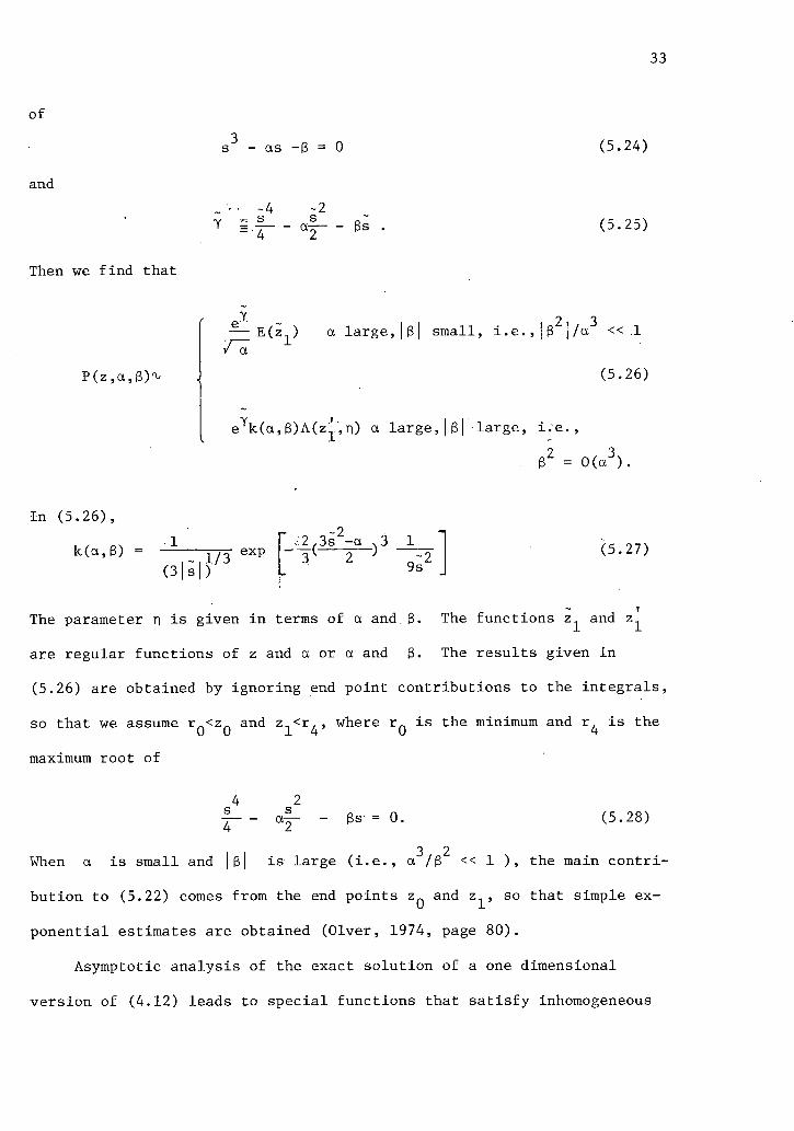
33
of
and
s - a s -6 = 0
. ••• • ~4 ~2 Y s . | _ - a | - - B s
(5.24)
(5.25)
Then we find that
P ( z , a , B ) ^
,2. , 3 E(z ) a l a r g e , | 3 | s m a l l , i . e . , | B | / a « .1
(5.26)
e Yk(a ,B)A(z 1 ' ,n) a large, ] B | large, i.e., 2 3
B Z = 0(a J).
In (5.26),
k ( a , B ) = (3|s|)
1/3 exp _;2,3s - a 3
3 2 ;
9s 2
(5.27)
The parameter n is given in terms of a and. B . The functions z^ and z^
are regular functions of z and a or a and B . The results given in
(5.26) are obtained by ignoring end point contributions to the integrals,
so that we assume r <z_ and z <r,, where r„ is the minimum and r. i s the 0 0 1 4 0 4
maximum root of
4 2 s s Is- = 0. (5.28)
3,„2 When a is small and |B| is large (i.e., a /B << 1 ), the main contri
bution to (5.22) comes from the end points ZQ and z^, so that simple ex
ponential estimates are obtained (Olver, 1974, page 80).
Asymptotic analysis of the exact solution of a one dimensional
version of (4.12) leads to special functions that satisfy inhomogeneous

34
versions of (5.12), (5.18) and (5.23). The results given above
indicate that i t may be possible to solve the two dimensional problems
(4.10), (4.12) by an asymptotic method. The separatrix would be
surrounded by a boundary layer. Outside of the boundary layer u(x)
is approximately constant and inside the boundary layer, u(x)
changes rapidly. The width of the boundary layer w i l l depend upon
the type of deterministic dynamics. Consequently, we shall construct
formal asymptotic solutions of the backward equation in the normal,
marginal and c r i t i c a l cases. Although the solutions w i l l be formal,
the numerical results presented in Chapter 5 indicate that they are
satisfactory.
The results obtained in this section could also have been obtained
by the use of the method of matched asymptotic expansions (Mayfeh, 1973).

35
Chapter 2. Asymptotic Solution of the First Exit Problem in the
Normal Case
6. Normal Type Dynamical Systems
The reduced (e = 0) deterministic system corresponding to
equation (4.10),
x 1 = b 1(x), (6.1)
is assumed to have three steady states, P^, P^, and P . Let
B = (b 1,.) denote the matrix obtained by linearizing b(x) and k 3 evaluating the result at P^ . We assume that B^ and have two
negative real eigenvalues and that P^ and P are bounded away
from the separatrix tube. The matrix B^ has one real positive and
one real negative eigenvalue. The eigenvector corresponding to the
negative eigenvalue has positive slope. A deterministic system
satisfying the above postulates w i l l be structurally similar to the
one sketched in Fig. 6.
x4-Fig. 6. The Normal Type Dynamical System

36
It is assumed that a(x) is bounded above and is positive
definite on the deterministic separatrix.
7. The Asymptotic Solution
The analysis of the one dimensional problem in §5 indicates that
a possible formal solution of the backward equation is
u(x) = I e ng n(x)E(^(x)//e") + e n + % h n ( x ) E ' (^//i) . (7.1)
In (7.1), E(z) is the Error integral:
E"(;z) = -zE'(z) z <_ z <_ z± . (7.2)
The limits z^, z^ are chosen so that (7.1) w i l l satisfy the boundary
conditions to within asymptotically small correction terms. The
ansatz (7.1) was used by Mangel and Ludwig (1977). The theory of that
paper is a special case of the theory presented in this chapter.
When derivatives of u(x) are evaluated, equation (7.2) is used
to replace E" and E" 1 by products of E' and ij///e . After
derivatives are evaluated and substituted into (4.10) terms are collected
according to powers of e . We obtain
0= I En " * ( g V ) ( b V . " 4~ <M^)E'0P/v^)
n=0 n i n a 1 3 n-1 i n-1. , , /-+ e (b g ± + — g + c g ± )E(\|)//e)
,, , /-. n+%r, i , n , i j n, , a 1 3 n, , n i , +El(i|)//e)e Hb h + a J g J) + — g + g c ty. (7.3)
- c h ^ + c h. - *a V ^ . + — h.. _. 1 _ hn
( ( W i ) 5 _ ) } .

37
In equation (7.3), i f the superscript of g n or h n is less than
zero, that term i s set equal to zero. The leading term, n = 0, is
composed of three parts and vanishes i f
i a l j
b \ - ^ i p ^ * = 0 (7.4)
b^J = 0 (7.5)
l A 0 _L 0, . i j 0. , 0 i j , , b h. H — g i i . . + a g.it. - h.a JM.
l 2 & r i i & i T j l y r i
+ g ° c S i - c V t t . - ^ ( ( ^ j ) = o . ( 7 - 6 )
Equation (7.4) is analogous to the eikonal equation of optics
(see §8). It i s obtained independently of g U(x) and h n(x) . Since
b 1 = dx 1/dt, equation (7.5) indicates that
dg° f f - = 0 . (7.7)
Thus g^ is constant on trajectories. In §8, we show that the
constant is the same on a l l trajectories. Once and g^ are
known, h^ can be calculated from equation (7.6). In §8,9 we
explic i t l y treat equations 7.4 - 7.6. Higher order terms are treated
in an analogous fashion (Appendix B).
Determination of ij; and g^: Contours of Probability
8.1. Determination of i K x )
2 The transformation <j> = -%i j ; converts equation (7.4) to

i a ± j
b f + ^ r - d>.dp. = 0 . (8.1)
Equation (8.1) i s the Hamilton-Jacobi equation or eikonal equation
(see also Cohen and Lewis, 1967; Ventcel and F r e i d l i n , 1970). It
corresponds to a Hamiltonian
H(x,p) = ~ a ^ p ^ + b ^ , (8.2)
and Lagrangian
L(x,x) = | a . . ( i 1 - b 1 ) ( i j - b j ) , (8.3)
where (a..)= (a"'""') 1 and
. i 8H x = T~ 3p ±
(8.4)
According to Hamilton-Jacobi theory, <|>(x) i s the minimum value of
the i n t e g r a l of the Lagrangian taken over a l l paths j o i n i n g x^
and x . If XQ i s the saddle point, then <j> = 0 on the separatrix,
since L(x,x) = 0 i f x± = b 1 . Thus <j> = = 0 on the separatrix.
Since equation (8.1) i s nonlinear, i t may have solutions i n
which 4>(x) i s non-zero on the separatrix. Consequently, by s e t t i n g
(f> = = 0 on S , we are imposing an extra condition on iKx) • This
condition can not be determined d i r e c t l y from equation (7.4) or (8.1).
If ip i s non-zero on S, then the f i r s t d e r i v a t i v e s of IJJ must
vanish on S . In t h i s case, i t i s not possible to construct a s o l u t i o n
(4.10) that approaches zero on one side of the separatrix and one
on the other side.
Equations (7.4) and (8.1) with i n i t i a l data on S represent
39
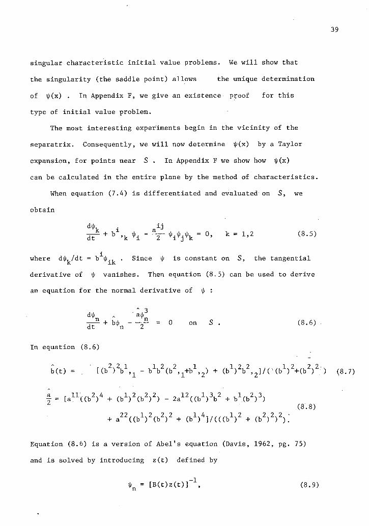
singular characteristic i n i t i a l value problems. We w i l l show that
the s i n g u l a r i t y (the saddle point) allows the unique determination
of ty(x) . In Appendix F, we give an existence proof for th i s
type of i n i t i a l value problem.
The most interesting experiments begin i n the v i c i n i t y of the
separatrix. Consequently, we w i l l now determine ip(x) by a Taylor
expansion, for points near 3 . In Appendix F we show how *Kx)
can be calculated i n the entire plane by the method of chara c t e r i s t i c s .
When equation (7.4) i s differentiated and evaluated on S, we
obtain
d \ i a ± j
ar + h - k * i - — W k - °> k = 1 ' 2 ( 8 - 5 )
where dip,/dt = b1^., . Since ty i s constant on S, the tangential
derivative of ty vanishes. Then equation (8.5) can be used to derive
an equation for the normal derivative of ty :
dty „ " aty^ 3-"- + bty ~ = 0 on 3 . (8.6) dt Yn 2
In equation (8.6)
b( t) = , U b V b 1 ^ - b V a 2 , ^ 1 , ^ + (bVb2 ,2]/( ( b V-Kb 2) 2) (8.7)
a 11.. .,2.4 . ,,1.2., 2.2. . 12. ,,1,3, 2 1 2.3. -n = [a ((b ) + (b ) (b ) ) - 2a ((b ) b + b (b ) )
(8.8) + a 2 2 ( ( b V(b 2) 2 + ( b 1 ) 4 ] / ( ( ( b 1 ) 2 + ( b 2 ) 2 ) 2 ) . '
Equation (8.6) i s a version of Abel's equation (Davis, 1962, pg. 75)
and i s solved by introducing z(t) defined by
tyn = [ B ( t ) z ( t ) ] _ 1 , (8.9)

where B'(t) = bB . The s o l u t i o n of (8.6) i s
* n ( t ) = a(s)exp t
a(s)exp|-2 j b(s')ds' ds| . (8.10)
Equation (8.10) s a t i s f i e s the condition
(8.11)
which i s consistent with (8.6) at the saddle point (where t = °° and
dij^/dt = 0} . The higher d e r i v a t i v e s of ty, up to order r can be
calculated i n an analogous fashion, i f deterministic equations are • „r' . C xn x.
8.2. Determination of z^, z^ and g^
We f i r s t suppose that the boundaries I and II are l e v e l
curves of ^ ( x ) , say IJJ = if^ on I and = on I I . We set
ZQ = ijjj. and z^ = i n equation (7.2). To leading order u = 0
on boundary I, and u = 1 on boundary II i f
g Q . (8.12)
In l i g h t of (7.7), g^ = l/Eity^/Ze) on a l l t r a j e c t o r i e s that
i n t e r s e c t boundary I I . Since a l l t r a j e c t o r i e s i n the lower half
plane i n t e r s e c t at = 1/E(if» .j.//e) on a l l those t r a j e c t o r i e s .
In p a r t i c u l a r , g^ has the above value on the t r a j e c t o r y from P^
to ?2 • Thus, gp has the above value on the t r a j e c t o r y from P^
to PQ . If t h i s were not so, equation (7.7) would be v i o l a t e d

41
when t is replaced by -t . Since a l l trajectories in the upper
half plane intersect at P Q , = 1/E(ty^/Ve) on a l l of these
trajectories. Thus, g^ is constant in the entire phase plane.
If ip(x) is not constant on I and II, then u(x) w i l l
not be 0 or 1 on the boundaries, but w i l l be close to 0 or 1
Let ty^, ty^ be the minimum and maximum values of ty on I . We
set z^ = <J/!j! . Then on I, u(x) is not zero, but
u(x) < g E(^ I//e) = g e ds (8.13)
An integration by parts yields
u(x) < 4 ^ — ^ -S ^ (8.14)
+ o ( e3 / 2 ) .
Thus, i f ty^ and ty^ are bounded away from 0, u(x) w i l l be
exponentially small on boundary I . This restriction i s an implicit
assumption about the boundaries.
If (JJ^J is the maximum value of ty on II, we set
EOj^/vT) (8.15)
An argument similar to the one above shows that on boundary II:
l-u(x) I < _ Jz
II
II i i i 0
T J s r I I (8.16)

where is the minimum value of iKx) on boundary II .
With the above choices of z^, z^ and g^, the ansatz (7.1)
w i l l satisfy the boundary conditions to within exponentially small
correction terms.
8.3. Contours of Probability
Once ij; and g^ are known, the leading term in the expansion
of u(x) is
u(x) <\, g°E(iKx)/v£) + 0(e*) . (8.17)
Since \\i vanishes on the separatrix, in a v i c i n i t y of the separatrix
iKx) = * (x )6n + 0(6n 2) (8.18) n s
where x g is a point on the separatrix and Sn is the distance
from x to x . s Contours of equal probability are obtained when i K x ) is a
constant. Thus, to leading order, we obtain contours at distances
<5n = l/tp from the separatrix.
9. Completion of the f i r s t term: Evaluation of h^
Since i|> = 0 on the separatrix, equation (7.6) becomes
dh° a l j ,0, , a l j , 0 0 i , , Q
Tt rh V j = "i-V " 8 c *± •
At the saddle point, dh^/dt vanishes. Equation (9.1) can then be
solved for h^(P^):

43
= K (9.2)
The solution of (9.1) which satisfies (9.2) is
i|>i. + c 1^ i]g°ds + K (9.3)
P(t)
where
p(s) = exp (9.4)
and K i s given by equation (9.2).
Once h^(t) is known on S, equation (7.6) can be used to
calculate h^ in the plane. Since the separatrix i s a characteristic
curve of (7.6), the problem as posed is a characteristic i n i t i a l
value problem. In Appendix A, we show how the above problem can be
converted to a noncharacteristic i n i t i a l value problem and h^
calculated everywhere in the plane. The existence proof for solutions
of (7.6), with i n i t i a l data on the separatrix is analogous to the
existence proof given in Appendix F.

44
Chapter 3. Asymptotic Solution of the First Exit Problem In
the Marginal Case
10. Marginal Type Dynamical Systems
The deterministic evolution of the macrovariables i s governed
by
x = b(x,n) (10.1)
where n is a parameter. Equation (10.1) may have three steady
states, Q (n) , Q-, (n) and P„ . Let B be the matrix (b 1,.) U 1 ^ K J
evaluated at Q Q ' ^1 ° r P2 (k = 0,1,2) . We assume that:
1) For a l l values of n, B 2 has two real negative
eigenvalues. Although may depend upon n , ¥^ is always bounded
away from the separatrix tube.
2) As n i 0, the distance between Q Q ( H ) and Q^(n)
decreases. When n = 0, and coalesce and annihilate each
other (i.e. when n < 0, (10.1) has one real and two complex steady
states).
3) When n > 0, B Q has two real negative eigenvalues
and B^ has one real positive and one real negative eigenvalue.
When n = 0, B^ = B^ has one zero and one real negative eigenvalue.
The eigenvector corresponding to the negative eigenvalue has positive
slope. The double point QQ(0)/Q^(0) i s called a saddle node
(Andronov et. a l . , 1973).
A deterministic system satisfying the above assumptions w i l l
be structurally similar to the system sketched in Fig. 7.

45
JC* x 1 x*-
n > 0 n = 0 n < 0
Fig. 7. Marginal Type Dynamical System
The above conditions can be reformulated by a change of coordinates. Define the y 1 axis in the direction of the eigen-
2
vector of the non-negative eigenvalue of . The y axis is
in the direction of the eigenvector of the negative eigenvalue of
B^, with the origin at . Then y = b(y,n) (10.2)
is the deterministic system in the new coordinates. The system is
of the marginal type i f :
1) det(b 1, j(Q 1,0)) = 0
2) b 1, 1(Q 1,0) = b 2, 1(Q 1,0) = 0 (10.3)

3) b 2, 2(Q l S0) + 0
4) b 1, n(Q 1,0) - b 2, n(Q 1,0) * 0 .
11. The Asymptotic Solution
11.1. Breakdown of the Error Approximation
If one wishes to use the theory of §8 to solve the backward
equation, then *Kx), the argument of the Error integral, must
satisfy
alJiJ):i|>. , b \ - — f ^ " * = 0 . (11.1)
In the marginal case, b(x) vanishes at two points QQ and .
In §7, we showed that ip(Q^) = 0 . It i s clear that ^(QQ) must
be less than . ip(Q^) • Thus, at Q , the ip^ must vanish or be
in f i n i t e and ip(x) is no longer a regular function. If ip(x)
is to be regular, the Error integral must be replaced by a more
complicated special function.
11.2. Uniform Solution in Terms of the Airy Integral
The analysis presented in §5 indicates that the uniform solution
of the backward equation in the marginal case can be given in terms
of the Airy integral and i t s derivative. In analogy to §7, we seek
a formal solution of (4.10) of the form
u(x) = I e ng n 0 O A 0 p/e 1 / 3, a/e 2 / 3) (11.2)
, n+2/3 ,n. 1/3 , 2/3. + e h (x)A' (IJJ/E , a/e ) .

47
In equation (11.2), the parameter a and functions *Kx), g n(x)
and h n(x) are to be determined. The function A(z,8) is the Airy
integral and satisfies
dz
When the derivatives of u(x) are evaluated, equation (11.3) is used 2 2/3
to replace A" by products of A' and (IJJ -a)/e . Following
Lynn and Keller (1970) we assume that a = _ a^e . (11.4)
After derivatives are evaluated and substituted into the backward
equation (4.10), terms are collected according to powers of e . We
obtain:
0= I e n" 1 / 3A'(g n-(^ 2-a 0)h n ) ( b S i-(^ 2-ct 0) 1^-n=0
+ I e A(b g ; L + — g ± j + c g ; L )
, r n+2/3,, , - i , n . i n , i , ,2 . n i , n - l + I e A (b h, + c g ^ - c ^ ( ^ "aQ^n + c h i
a1"' n i i n, a 1^ , n-1 .,2 . i j , n , + — 8 *ij + a g i * j + ~r h i j " ^ - a o ) a V j
- h n ^ ( ^ . ( U ; 2 - a 0 ) ) . (11.5)
+ "-T a k { h n + 1 " k ( b \ - ( ^ a 0 ) ^ ) + * 1 * j ( g n + 1 _ k -k=l ,,2 .,n+l-kN, , v / i , T.n-k , a 1 J
/ o un-k, (i|> -a Q)h )} + i a f e(c + — ( 2 h ± ip Ic X
. n+1 i j , ,, k-1 + h i|> )) + £ -y- * ,h ( 1 a.o. )) . i j k = 2 4 j = 1 J k 3

48
In equation (11.5), i f a superscript i s less than zero, that term is
set equal to zero.
The leading term (n=0) is composed of three parts and w i l l
vanish i f
i j o
b 1^. - ty±ty. (ty-aQ)= 0 (11.6)
b^J = 0 (11.7)
~ ai^T V j ( g ° " ^ 2 - a0
) h 0 ) + g°*ij ( 1 1 ' 8 )
+ c~ty^g* + c^ty^b®\^-O.Q) = 0 .
Equations (11.6, 7) were used in obtaining (11.8).
From equation (11.6), we see that ty(x) w i l l be a regular
function of x . The f i e l d b(x) vanishes at two points Q , . 2
We require that ty = ct at these two points. Since ip(Q^) > M Q Q )
for the problem as formulated, we set *K QQ) = ~^®Q ANC*
ip ( Q 1 ) = .
In §12-14, we explicitly treat (11.6 - 11.8). Higher order
terms can be treated in an analogous fashion (Appendix B).
12. Evaluation of the Parameter
1 3 2 3/2 The substitution <j> = - -j ty + a^ty ~ 3" A Q converts equation
(11.6) to the eikonal equation (8.1). An argument analogous to the
one in §8 shows that ty = V'OQ" on the entire separatrix S . The

49
parameter must be determined so that (11.6) is satisfied with
i n i t i a l data ip = v'cx on the separatrix and the additional condition
that ij; = -/ct^ at QQ . The one additional condition allows the
unique determination of .
The following iterative procedure can be used to determine .
An i n i t i a l choice of a^, is made. We set = -/a^^ at QQ .
Equation (11.6) is then solved by the method of characteristics
(Courant, 1 9 6 2 ) . When the method of characteristics is used, the
phase plane is covered by a family of trajectories called rays. The
rays are generated from the system of ordinary differential equations
dx 1 i a l j 2
. P. ( 1 2 . 2 ) ds ds x
d p k , i , „ i i , , ' k , , 2 ds = " b 1 ^ p ± + 2a±3 tV^Vy. + — 2 — P i P j ( ^ " a o ) 5 ( 1 2 . 3 )
where p. = ip. . Some of the rays emanating from Q w i l l hit the
separatrix S . If ip 4- A Q ^ O N then must be replaced
by an improved estimate of a^, aQ^^ • T n e method of false position
(Dennis and More, 1977) can be used to calculate increments in .
The above procedure can be repeated u n t i l is determined to any
desired accuracy. As the estimates aQ n^ approach the true value
01Q, the rays w i l l begin to bend and run parallel to the separatrix,
which is i t s e l f a ray. An indication that a ray is approaching the
separatrix is that b"N|> = t —> 0 . This criterion can be used in
numerical determination of .

50
An equivalent procedure would follow rays that emanate from the
saddle and approach QQ • If ty does not approach -/ot^^ as
the ray approaches QQ, the estimate of must be modified. A
pr i o r i i t is not clear which technique is preferable. The decision
must be made on the basis of practicality. The calculations described
in Chapter 5 used the f i r s t technique.
13. Determination of ty and g^: Contours of Probability
A procedure analogous to the one in §8 yields the following
equation for ^ ( t ) on S :
- j - " - + bty - y^TT aty = 0 . (13.1) dt n 0 n
When 01Q > 0, i.e. the two points have not coalesced, equation
(13.1) can be treated exactly as (§;6) was. In Appendix D we show
that the constructions given here and in §14 are regular at the
marginal bifurcation.
Similarly, the values of ZQ, Z^ and gQ can be determined
as in §8.2, except that the Error integral i s replaced by the
incomplete Airy integral. When g^ is evaluated, the expansion
of the Airy integral (5.19) can be used to simplify the evaluation
of g .
Once ty and g^ are known, the leading part of the formal
expansion for the f i r s t exit probability i s
u(x) ^ g 0 A 0 K x ) / £1 / 3 , V ^ 2 7 3 ) + 0 ( e 2 / 3 ) ' ( 1 3 ' 2 )
Equation (13.2) can be used to generate contours of equal probability.
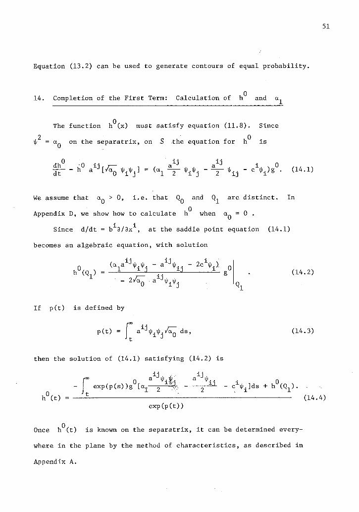
14. Completion of the First Term: Calculation of h^ and a
The function h^(x) must satisfy equation (11.8). Since
C(Q on the separatrix, on S the equation for h^ is
,,0 i j i j dh -0 i j r i — , , n / a , , a * i j " c \ ) § ° - ( 1 4 - 1 )
We assume that > 0, i.e. that QQ and are distinct. In
Appendix D, we show how to calculate h^ when = 0 .
Since d/dt = b"L9/8x1, at the saddle point equation (14.1)
becomes an algebraic equation, with solution
ij,,, ... _ i j . (a a - a > - 2c ty.\ h (Q ) = _ 1 -1 g
- 2/a_ a \b . ib . - 2/a_ • a 1 3ib ,\b . 0 (14.2)
If p(t) is defined by
p(t) = a 1 3 il>. iii. /al ds, (14.3)
then the solution of (14.1) satisfying (14.2) is
h°(t) = e x p ( p ( s ) ) g [cx^—2
n a^ib.ty. a±2ty O r i-h.
2 1 3 - c 1ip ±]ds h°( Q l)
(14.4) exp(p(t))
Once h^(t) is known on the separatrix, i t can be determined every
where in the plane by the method of characteristics, as described in
Appendix A.

5 2
The parameter i s s t i l l undetermined. It can be approxi
mately calculated as follows. The f i e l d b(x) vanishes at QQ,
where \\i = • At Q , equation (14.1) becomes
0 ( a a 1 J ^ i K - a 1 J i p - 2c 1* ) h U(Q ) = -— M ^- g U
U 2>/oT a J * . i j J . (14.5)
0 r i r j x0
When QQ and are close together, we determine h^ at QQ by
a Taylor expansion
h°(Q 0) _. h°(Q 1) + v.6x\ (14.6)
where v. = Sh^/Bx1]^ . The parameter an is chosen so that ' i lQ 1 1
equations (14.5) and (14.6) agree.
A more exact determination of uses the method of
characteristics, as the calculation of did. As described in
Appendix A, a manifold S' can be determined on which (14.1) is
not a characteristic i n i t i a l value problem. Then, equation ( 1 4 . 1 )
can be solved by the method of characteristics, starting at .
When a ray reaches QQ, h^ should have the value given in ( 1 4 . 5 ) .
If the value of h^ at QQ, when calculated by the method of
characteristics, is not the same as the value given in ( 1 4 . 5 ) , then
the estimate of must be modified. The method of false position
can be used to calculate the iterates of .

53
Chapter 4: Asymptotic Solution of the First Exit Problem in the
Cr i t i c a l Case-
15. C r i t i c a l Type Dynamical Systems
The macrovariables evolve according to a deterministic kinetic
equation
x = b(x,n,S) (15.1)
where n, 6 are one dimensional parameters. The entire bifurcation
set of equation (15.1) is s t i l l unknown (Arnold, 1972). The physical
systems of interest here motivate the following assumptions:
1) For some values of r\, <5, (15.1) has three steady
states PQ(n,<5), P (ri><5) and • A l l three steady states
are contained in the separatrix tube. If B, = (b 1,.) evaluated
at P^, then when the three steady states are distinct, B^ and
B 2 have real negative eigenvalues. B^ has one real negative and
one real positive eigenvalue. The eigenvector corresponding to
the negative eigenvalue has positive slope.
2) As n, 6 vary, two of the steady states may coalesce
and annihilate each other. This behavior i s analogous to the
marginal bifurcation.
3) As ri, 8 vary, a l l three steady states may move together
and coalesce when n = & = 0 . At the c r i t i c a l bifurcation, B = (b"t.)
has a zero eigenvalue. We assume that the steady state remaining
after the c r i t i c a l bifurcation is a stable steady state.

Fig. 8. Bifurcations of a C r i t i c a l Type Dynamical System

The above properties can be restated in terms of a new coordinate
system as follows. The y"'" axis i s in the direction of the eigen-2
vector of the non negative eigenvalue of B^ . The y axis i s in
the direction of the eigenvector of the negative eigenvalue, with the
origin at P^ . The deterministic evolution i s then
f = b(y,n,<5) . (15.2)
A dynamical system is a c r i t i c a l type system i f :
1) det(b 1, j(P 1,0,0)) = 0 2) b 1, 1(P 1,0,0) = b 2, 1(P 1,0,0)
= b 1, 1 1(P 1,0,0) = b 2, n(P 1,0,0) = 0 (15.3)
3) b 2, 2(P 1,0,0) j 0
4) b 1 , 1 1 1 - b 2> l l i y o . - :
16. The Asymptotic Solution
16.1. Breakdown of Solutions Using the Airy Integral
If the theory of Chapter 3 were used in the c r i t i c a l case, the
argument of the Airy integral would have to satisfy
i j o b ^ ± - *±*j C * V = 0 ' (16.1)
Since the deterministic f i e l d now vanishes at three points in the
separatrix tube, expression (16.1) indicates that *(x) w i l l not
be regular at the third steady state. If we wish to construct a
solution in which ip(x) is regular, the Airy integral must be

replaced by a more complicated special function.
16.2. Uniform Solution in terms of the Pearcey Integral
The analysis in §5 and results in Chapters 2, 3 indicate that
a possible formal solution of the backward equation in the c r i t i c a l
case i s
u(x) = I £ngn(x)P(Mx)/e1/4, a/e 1 / 2, B/ £
3 / 4) (16.2)
+ en + 3 / 4h n(x)P ' (Kx)/ £
1 / 4 , a / £1 / 2 , B/ E
3 / 4)
where the parameters a, B and functions ^(x), h n(x) and g n(x)
are to be determined. The function P(z,a,B) is the Pearcey
integral, satisfying
2 d P, , 3 n.dP(z,a,B) ~s —jCz.a.g) = (z -az-B) ^d'z
, W J zQ <_ z <_ z . (16.3) dz
When the derivatives of u(x) are evaluated, equation (16.3) is 3 3/4
used to replace P'.' by products of P' and (i[i -atp-g)/e . We
assume that a and 8 have asymptotic expansions of the form
a = I e k a k B = I B ^ . (16.4)
After derivatives of u(x) are evaluated and substituted into the
backward equation (4.10), terms are collected according to powers
of e . We obtain

57
0 = I en-1/S.(gn+h
n(^3_ao^-eo))(b%.+-^ tyty (ty3-aQi,-^Q)) n=0 3
v n „ , , i n a 1 3 n-1 i n-1. + I £ P(b g + - X - g + C g )
n=0 J
v n+3/4 , r , i , n , i n , i n-1 . ,n i , , , 3 , a \ + I e 7 P'{b h ± + c g± + c h ± + h c.tyAty - a Q i | j - B 0 )
K. -L
hn + 1- k
( l (, 3_ a^-3 o) + h n + 1 _ k ( b % i + ^ V j } ( l 6 - 5 )
n+1 i j k-1
+ j 2 V V j h v ^ v V ^ - j ^ k - j ^ n , 11 , 1 v • , . „ w 1, , n-k a n-k, , ,n-k, . . - _ (i|)otk+ek)(c - — (2h ± ^ + h ty±p)
k. X n i j 1 V a J , , , n-k,
k=l k ^ 1 J
In equation (16.5), i f a superscript is less than zero, that term i s
set equal to zero.
The f i r s t term in (16.5) i s composed of three parts and w i l l
vanish i f
i a i j 3 b * i + % ~ ^ - j ^ V V = ° (16.6)
bV? = 0 (16.7) °i
b\°± + g\. + 0 p 3 - a 0 i j ; - 3 0 ) a l j h ^ .
+ ~ ~ h % (ty3-aQty-3Q) + h° - ty±ty. ( 3 i p 2 - a Q ) . (16.8)
- ( ^ a 1 + 8 1)f 0 ( ' p,l ) + . g 0c 1ij; i + c 1 ^ i h ° ( < | / 3 - a 0 ^ - 8 0 ) = 0 ,

58
where we have denoted
f n(^,k) = T ^ ^ ^ ( g ^ + h n + 1 - k ( * 3 - V - B 0 ) ) k _ 1
± i (16.9) + h n + 1 " k ( b i * i + i ^ * . (ip 3-a 0*-6 0) ) .
The f i e l d b(x) vanishes at P Q, P 1 and P 2 . The function *(x) 3
w i l l remain regular i f * - a^ip - BQ vanishes at the points where
b(x) vanishes. Let _ ^-^ H ^ 2 denote the ordered roots of
* 3 - aQip - BQ = 0 . (16.10)
We then set <KPQ) = "KP^ = ^ and *(P 2) = * 2 .
In §18-19 we treat equations (16.6 - 8 ) explicitly. Higher
order terms are discussed in Appendix B.
17. Determination of the Parameters and 8Q
1 A 2 1 A' ~ 2 The transformation <j> = * - a^ip /2 - & ~ "4 + " o ^ l ^ 2 +
8Q*^ converts equation (16.6) to the eikonal equation (8.1). An
argument using Hamilton-Jacobi theory, as in §8, shows that * = ^
on the entire separatrix.
Equation (16.6) must be solved with i n i t i a l data on the separatrix
and the two extra conditions ^( PQ) = *J>Q a n d ^(P 2) = ^ 2 ' T h e t w o
extra conditions allow the unique determination of and BQ .
As in §12, an iterative procedure is used to determine and 8Q •
I n i t i a l estimates, a n <* » a r e u s e c ^ "*"n (16.6).
Equation (16.6) Is solved by the method of characteristics, starting

59
close to the saddle point where ty = ty^ and ty^ is the middle root
of
* 3 - a < % - g<°> - 0 . (17.1)
Some rays emanating from P^ w i l l approach P^, others w i l l
approach • As PQ i s approached, ty should approach ty^; as
P^ i s approached ty should approach ty^ • If *KPQ) , i K ^ ^ a r e
not ipQ, ty^j then the values of the parameters must be modified.
The method of false position can be used to calculate iterates of
CXQ and 6 . This procedure can be repeated un t i l (XQ and 8Q
are determined to any order of accuracy.
18. Determination of ty and g^: Contours of Probability
Using the procedure outlined in §8, the following equation can
be derived for ^'(t) o n t n e separatrix
dty „ " q ~ 2
dT + hK + V K ° K ~ a o } = ° - ( 1 8 - 1 )
We assume that the three points have not coalesced, so that ty and
CXQ are not both zero. In Appendix E we show that the constructions
in §17-19 are regular at the c r i t i c a l bifurcation. Equation (18.1)
can be treated exactly as (8.6) was treated.
Similarly, ZQ, Z^ and g^ can be calculated as in §8.2, except
that the error integral i s replaced by the incomplete Pearcey integral.
When g^ is evaluated, the expansions (5.26) can be used to simplify
numerical calculation.

Once a.Q, BQ, ty and g are known, the leading term in the
formal expansion of u is
u(x) ^ g°T>(ty/e1/A, a 0/e 1 / 2, B 0/e 3 / 4) + 0(e 3 / 4 ) . (18.2)
Equation (18.2) can be used to generate contours of equal probability.
19. Completion of the f i r s t term: Calculation of h , and B
The function h^ must be determined from equation (16.8). On 3
the separatrix, where ty = ty^ and ty - a^ty - BQ vanishes, (16.8 )
becomes dh° . , 0 a ± j a 1 J 0 0 i , _ _ + h _ _ V j ( 3 * r o 0 ) = OP-^+B^ — g ty±ty. ~ g c ty±
a 1 J 0 2
(19.1)
Since d/dt = b 13/3x 1, at the saddle point P^ equation (19.1)
becomes
OP a +g )a 2ty ty - 2c ty -a 2ty ) Q
h U(P ) = I J 1 U_ gtf (3ip -a )a Jty ty
(19.2)
If p(t) is defined by
P(t) = ' ~2 a 1 J
Otyj-a^^- i p ^ d s , (19.3)
and
i j . a 1 Jip.. f(t) =(-0P 1 a 1 +B 1 )^ 2 - ty±ty. + c1ty± + 2
1 3 )g U, (19.4)

61
the solution of (19.1) satisfying (19.2) i s
r -P( S> 0 f (s)e ds+ h (P ) h°(t) = — ; . (19.5)
expC-p.(t)]
Once h^(t) is known on the separatrix, i t can be determined every
where in the plane, by the method of characteristics, as described
in Appendix A.
The parameters ct and 6 are s t i l l undetermined. They can
be determined by using the method of characteristics, in a manner
analogous to the calculation of and BQ . As described in
Appendix A, a new manifold S' can be constructed, with h^ known
on S', so that (16.8) i s not a characteristic i n i t i a l value problem.
Then (16.8) can be solved by the method of characteristics. Some
rays emanating from S' w i l l approach PQ or F^, where h^ must
have the value
((* a +3,)a V.iK - 2c * - a V..)g h°(P ) = i j J 1 12-
(3^-a )a 1 3i|; * , k=l,2. (19.6)
P,
If the value of h^ at P , when calculated by the method of
characteristics, is not the same as the value determined from (19.6),
then the estimates of and B must be improved. The method of
false position can be used to calculate iterates of and B •

62
20. Two Complex Steady States with Small Imaginary Parts
When n < 0 (marginal case) or n < 0, 6 < 0 ( c r i t i c a l case)
only one real steady state exists. There w i l l be two complex steady
states. If the imaginary parts of the complex steady states are
small, then the linear part of the deterministic equations about the
real steady state w i l l be small. Consequently, the dynamics at the
steady state are almost completely nonlinear. We thus expect that
the Error integral, which corresponds to nonvanishing linear dynamics,
w i l l not provide an adequate asymptotic solution of the f i r s t exit
problem. The Pearcey integral, however, can be used to provide an
adequate asymptotic solution.
When the ansatz (16.2) i s used, the function *(x) must satisfy
(16.6). in order to determine and BQ by the method of
characteristics, complex rays would be needed. An easier, although
less accurate, technique uses power series for a ,.BQ • In
Appendix E, we derive power series of the form
= I A . . n V (20.1) 0 . . in i,3
r . . A 3 BQ = I B N <5 . (20.2)
i,3
The power series extend up to order r, in n and 6, i f the
deterministic equations are 0 in n and 6 . Since we are using
power series, the results given in this section are valid only in
a neighborhood of the origin in (n,6) space.

63
The value of IJJ on the separatrix i s tp^, where ij> is the
real root of
* 3 - cyj - B Q = 0 . (20.3)
Using the technique in §18, we can calculate the value of Y in a
neighborhood of the separatrix by a Taylor expansion. The value of
g^ can be determined as described in §8.2. Thus, the leading
term of the f i r s t exit probability is
u(x) <x, g°P(<Kx)/ e1 / 4, V ^ 1 7 2 . V e 3 / 4 ) 1 ( 2 0 > 4 )
Our solution i s approximate in the following sense. Since a^, BQ
are only given as power series, equation (16.6) is not satisfied
identically, but must be replaced by
i a l J V i 3 r+1 r+1
Let L indicate the backward operator. Then, our formal result
w i l l satisfy the backward operator to an order of en<$ :
Lu = 0 ( e ~ 1 / 4 ( n r + 1 + <S r + 1)). . . (20.5)
The estimate (20.5) indicates how close n, 6 must be to the origin
for our ansatz to be valid. Unlike a l l previous results, which were
independent of e, the validity of the extension presented in this
section is dependent upon e .

64
Chpater 5. Fluctuation Effects on Substrate Inhibited Reactions
21. Multiple Steady States in Enzyme Reactions
The experiments ' of H. Degn (1968) conclusively demonstrated
that multiple stable steady states actually can be observed. In
his experiments, Degn was concerned with observing the multiple steady
states and not with fluctuation effects. It is clear, however, that
his techniques could be used to study fluctuation effects at the
unstable steady state. In this chapter, we study fluctuation effects
on a substrate inhibited reaction. Our choice of model was motivated
by Degn's experiments, but is not meant to correspond to the
exp er iment s exac t l y .
21.1. Deterministic Kinetic Equations
In this section, we develop a model of Degn's experiments. The
model has the following features.
1) A reaction vessel of volume V can exchange substrate '1'
with an external reservoir of volume V .
2) Substrate '1' i s converted into product by a substrate
inhibited enzyme. The concentration of substrate '1' in the reservoir
i s x"*": or X"'" molecules. An example of this reaction i s the r r oxidation (x^ being l ^ ] ) of NADH catalyzed by horse radish
peroxidase.
3) Substrate '2' is continually fed into the reaction
vessel, at rate a, and reacts with substrate The reaction
is catalyzed by an enzyme that obeys the usual Michaelis-Menten

65
mechanism (White et. a l . , 1969). An example of this reaction is
the oxidation of glucose, catalyzed by glucose oxidase.
The elementary steps involved in these reactions are
1 1 1 1 1 a) X X + E X ——^—KX E )
-1
1 1 1 3 1 1 b) ( x V ) + E J> ( x V )
k-3
c) . x V - ^ U E 1 + P 1
I 1 ? 9 1 1 2 2
d) x 1 + x z + E ZF > ( X V E Z )
- l 1 2 2 ^ 2 2 2
e) ( X V E Z ) — ^ E + P^
(21.1)
1 k 1 f) x 1 — : i X R
k
In order to derive the kinetic equations for the concentrations of 1 2
X and X , we use the Michaelis-Menten assumption (White et. a l . ,
1969). Nondimensional concentration variables are i , . [concentration of species i at time t] / 0 1 „ N
X (t) = -r-: 7 — 7 E : : Z~~ • (21.2) [concentration of species l at OJ
1 2
Then the kinetic equations for x and x are (Degn, 1968,
Higgins, 1967)

(21.3)
- x 2x^"( Z ^ / x ^ x ^ Z ^ )
^ _ I+ ^ 2 ) 2 1
10 20„ + x x
X X -L
/ x 1 0 x 2 0 / ) x = a — . (21.4)
(£_ I+£ 2) o l + x x 10 20„ x x -t^
In the above equations, x"^ is the i n i t i a l concentration of species
i . We choose the following values of the parameters: a = .09,
x 1 0 = x 2 0 = 10~7M, k = 1.2 x 10 7 £/M-sec, k =M2 sec" 1,
k^ = 1.68 sec \ k^ = 1.3 x 10^ M 2 sec \ k_^ = .01 sec
Z ^ = 0 sec \ Z^/Z^x^x^ = .1 . The values of x*" and k^
roughly correspond to Chance's (1951) experimental data. The Z.
were chosen as "reasonable" estimates, since no data were available.
With these choices, we obtain
1 12 1 - 1 4x 1 1 x x x = r 1 + k ( X r - ~ x ) " T T (21.5)
1.5 + x X + 13(x) 1 + lOx x
? 1 2
x = .09 - X X 1 2 . (21.6)
1 + lOx x
We assume that e=100 and the 'volume' V=l/e". Equations;

(21.5,6) are model equations that exhibit the marginal and c r i t i c a l
b i f u r c a t i o n s . They are not meant to simulate a p a r t i c u l a r set of
experiments. Since the rate constants of enzyme preparations vary
widely, t h i s appears to be a reasonable approach. We w i l l r e f e r to 1 2
(x ,x ) as concentration v a r i a b l e s . We w i l l treat V as a non-
dimensional quantity and treat X 1 = Vx 1 as a v a r i a b l e corresponding
to the number of "molecules".
21.2. Stochastic Model of the Enzyme Reactions
In the stochastic approach, the natural random v a r i a b l e s are the
numbers of molecules of species 1 and 2 i n the reaction vessel at
time t, X"*" and X^ . The concentrations are then ic 1 = X 1/V .
From the reaction mechanism (21.1), t r a n s i t i o n p r o b a b i l i t i e s can be
constructed. These are p r o b a b i l i t i e s i n a 5 dimensional space 1 2 1 2 1 1
(X ,X ,E ,E ,(X E ) ) . In order to be consistent, we must apply the Michaelis-Menten assumption to these p r o b a b i l i t i e s ; we replace 1 2 1 1
E ,E and (X E ) by t h e i r steady state values. Once t h i s replace
ment i s performed, the t r a n s i t i o n p r o b a b i l i t i e s w i l l be given s o l e l y
~1 ~2
i n terms of X and X . By using the Michaelis-Menten assumption,
we are t r e a t i n g the enzyme concentrations as parameters rather than
v a r i a b l e s . Thus, we are assuming that f l u c t u a t i o n s i n enzyme con
centration can be ignored i n comparison to f l u c t u a t i o n s i n substrate
concentration. This assumption i s consistent with the work of Heyde
and Heyde (1971) . They:~f ound that the steady state f l u c t u a t i o n s i n
enzyme concentration were 10 +^ - 10 +^ times smaller than the

68
fluctuations in substrate concentration.
When the Michaelis-Menten assumption is used, the transition
probabilities for AX1 = X 1(t+At) - X 1(t) are
Pr{AX1=l, AX2=0|x1(t)=X1} = — At + o(At) (21.7) V
Pr{AX1=-l, AX2=0|x1(t)=X1} = 1.4X1
+ + X 1* 2
1 1 2 V 2 1 1 2 1.5V+X +13(X ) V +10 X X
+ o(At) (21.8)
At
P r { A X 2 = - l , A X 1 = 0 | x i ( t ) = X i } = 9 + o ( A t ) (21.9) 2 1 2 V +10X X
Pr{AX2=l, AX 1=0 |x 1(t)=X 1} = .09VAt + o(At) . (21.10)
In Chapter 1, we introduced the infinitesimal covariance e(a J) and
pointed outl:that since the stochastic kinetic equation was not derived
from f i r s t principles, we need to provide a prescription for the
calculation of e(a 1 J) . We shall now provide one such prescription
by using the birth and death approach to chemical kinetics. One can
obtain a result identical to ours by using Keizer's technique,
(Keizer, 197.5), which does not use the birth and death
approach. Since none of the boundaries are singular,
a change in the method used to calculate e(a1~') w i l l change some
quantitative details, but w i l l leave the qualitative results unchanged.
Instead of the kinetic equation (4.5), consider the kinetic
equation
dx 1 = b a(x)dt + /ea 1 J dW. . (21.11) 3

69
In (21.11), W(t) is the Wiener process. The functions b 1 and ea1"1
have the simple interpretation (Feller, 1971):
b 1 = lim j-E{(x 1(t+At)-x : L(t)) 1Jx k(t) = x k = l,...,n} (21.12) At+0
ea l j = lim ^E{ (x 1(t+At)-x 1(t) ) (x^ (t+At)-xj (t))|x k(t) = x k = 1,... ,n}. (21.13) At->0 fc
Equations (21.12,13) are the Ito interpretation of equation (21.11)
(Nelson (1967), Arnold (1974)). Using the transition probabilities
(21.7-10) we can easily calculate the covariance e(a 1 ; ]) . This procedure
yields a result analogous to that obtained by the use of Keizer's
fluctuation-dissipation postulates (Keizer, 197.5). McQuarrie (1967)
would calculate the covariance e(a"L~') in a manner identical to the
one described above. Kubo et. a l . . (1973) and Matsuo (1977) also-use
similar procedures.
A white noise equation such as (21.11) can never really represent
a physical process. However, such equations are used almost uniformly
by physical scientists (e.g. Landau and Lifshitz (1959), (1968), Ma (1976)),
based on the idea that Y(s) has a negligible correlation time. We
realize that (21.11) is an idealization of equation (4.5). Following
Wong and Zakai (1965) , we w i l l give a white noise interpretation to
(4.5). Consider a sequence of mixing processes Y n ( r ) , which
converge to W(T) as n — y °° . If the stochastic variable i s x n(t;x)>
then as n —>• », x*1 —*• x where x satisfies the Ito equation (Wong
and Zakai (1965))
dx 1 = (b^x) eaXhdt + /ea 1 : i dW. . (21.14) 9xJ J

70
We shall use (21.14) as an approximation to (4.5). The backward
equation corresponding to (21.14) is
ST ea 1 3 , i , i . ufc = - 2 — u + (b +ec )u ±, (21.15)
where c""" = -r a 1 3 , . The backward equation corresponding to (21.11) 4 j
is
WN ea 1 3 , , i u = — - — u. . + b u. t 2 i j x (21r16)
In §22, one dimensional versions of (22.15,16) are compared. The
results of §22 indicate that for the problems of interest here, the
choice of stochastic calculus is not important. Consequently,
equation (21.14) is a useful approximation to (4.5).
The deterministic kinetic equations are given in terms of the
"concentration" variable x 1 ( t ) . When the transition probabilities
are rewritten in .terms of the concentration variables, the infinitesimal
covariance is
ea(x) = (100)'
; ( x 1 + li x)x
(A 2 + y 2)x (21.17)
where
1 r
y i X =
1.4x 1 1 2 1.5 + x + 13(x)
i 1 2
, , 1 • X X + kx H 1 2 1 + lOx x
(21.18a)
(21.18b)

71
X 2x 2 ^ .09 (21.19a)
o 1 2
y x Z = X X . (21.19b) 1 + lOx x
When the transition probabilities are used to calculate the infinitesimal
d r i f t b 1 ( x ) , we find
b 1(x) = - ~ ( ^ - H ^ x l (21.20)
b 2(x) = rjjfi (X 2 - H 2)x 2 . (21.21)
A rescaling of time then yields x 1 = b 1(x), so that the mean
stochastic motion and the law of mass action agree.
The covariance (21.17) and d r i f t (21.20,21) were used in a l l of
the calculations reported in this chapter.
22. Exact and Asymptotic Solutions of the Backward Equation
In this section, we assume that the concentration of species 2 2
is subject to perfect control, so that x is always at i t s steady . 2
value. When x =0, equation (21.5) becomes x 1 = z-j - kx 1 + (kx1-.09) = b(x1,n,6) . (22.1)
1.5 + x + 13(x X) r
In the sequel, we drop the superscript 1 on x"*" . When k = .0968493
and kx^ - .09 = .182033, equation (22.1) exhibits the c r i t i c a l
bifurcation (b = b' = b" = 0 at the steady state).

72
The backward equation, i f the non-white process is used, is
£ a ^ x ) u + bu + ecu = 0, (22.2) 2 xx x x
1 -2 where b(x) is given by (22.1), c = a^, e = 10 and
a(x) = +-kx .+ kx + .09 . (22.3) 1.5 + x + 13x r
ST We denote the solution of (22.2) by u (x). When a white noise approximation is used, (22.2) i s replaced by an equation in which
WN
c = 0 . We denote the solution of that equation by u
The unstable steady state is denoted by . The boundary
conditions for (22.2) are u ( xu ~ «4) = 0 and u ( x
u + «4) = 1 .
When b(x) has only one steady state, x g, the boundary conditions
are u(x - .4) = 0 and u(x + .4) = 1 . s s
A l l the exact solutions were calculated by a fourth order Runge
Kutta routine. The function ip(x), the argument of the special
function, w i l l satisfy bip - f f ( < J J)* 2 = 0, (22.4)
X —• X
2 3
where f(ip) = ip, ip ~ aQ o r + aQ^ + ^y' l n n o r m a l > marginal or
c r i t i c a l case respectively. At .the unstable steady state, i/» = * »
where f(ip„) = 0 . Solving (22.4) yields s
2b' 1/2 ip = (—rr) except at the bifurcations, (22.5) X 3.T.
ip = (r^)^~^ marginal bifurcation (22.6) X e l l

73
\p = ( 2 b,,,)"^ 4 c r i t i c a l bifurcation. (22.7)
Equations (22.5-7) were used in the calculation of ip(x)
A) The Normal Case
Values of parameters corresponding to the normal case are k = .038,
kx^ = .2225. The flow corresponding to (22.1) is sketched below:
0 .196 u=0 .878 u=l 2.34
In Table I, we compare the exact, white noise and 'mixing'.solutions of
(22.2) with the asymptotic solution of (22.2), using the theory
developed in Chapter 2. The agreement between the exact and asymptotic
solutions is excellent. This is to be expected, since the asymptotic
ansatz was based on the expansion of a one dimensional problem.
B) The Marginal Case
Values of parameters corresponding to the marginal case are
k = .0533, kx r = .24898 . The flow of (22.1) is sketched below:
0 u=0 .3169 .5266 u 1
In Table II, we compare the exact solutions with the asymptotic
solutions using the theory"developed in Chapters 2 (u^ r r° r) and Ail? v
3(u ). The results clearly indicate the breakdown of the Error
integral, but the success of the theory that uses the Airy integral.

74
Table I
Exact and Asymptotic Solutions in the Normal Case
EXACT ASYMPTOTIC
.WN u ST u % d i f f . WN u % d i f f ST
u **
% d i f f
.878 .47262 .47097 0.3 .47304 0.1 .47101 0.1
.978 .68808 .68675 0.2 .68732 0.1 .68458 0.3
1.078 .84730 .84650 0.1 .84510 0.3 .84333 0.4
.778 .26257 .26112 0.6 .26218 0.2 .25910 0.8
.678 .10814 .10729 0.8 .10782 0.3 .10606 1.1
l u ^ - u 8 1 ! % d i f f = -> u .ST
x 100
, , exact asymptotic ** u — u % d i f f = . . . 1 x 100
u asymptotic
These definitions are used in Tables I - V .

75
Table II
Exact and Asymptotic Solutions in the Marginal Case
x EXACT ASYMPTOTIC
ERROR AIRY
WN u ST u % d i f f WN u % d i f f WN u % d i f f ST
u % diff
.5266 .71003 .71185 .2 .50000 42 .71298 .4 .71426 0.3
.6266 .83243 .83048 .2 .69140 20 .82215 1.3 .83500 0.5
.7266 .92219 .92133 .1 .84134 9.6 .92833 .7 .92949 0.7
.4266 .58959 .59536 1.0 .30860 91 .59708 1.3 .59492 0.1
.3266 .48614 .48872 .5 .15866 206 .49105 1.1 .49394 1.1

C) The C r i t i c a l Case
Values of parameters corresponding to the c r i t i c a l case are
k = .08125 and kx r = .261199. The flow of (22.1) is sketched
below:
0 u=0 .3563 .7024 .9715 u=l
In Table III, the exact solutions are compared with the asymptotic
solution using the theory of Chapter 4.
The widening of the boundary layer around the unstable steady
state as the type of deterministic system changes is apparent in
Tables I-III. For instance, in the interval [ x ^ - . l , x +.1], u(x)
increases by .42551 in the normal case, but only by .27620 in
the c r i t i c a l case.
D) The C r i t i c a l Bifurcation
Values of parameters corresponding to the c r i t i c a l bifurcation
are k = .0968493, kx r = .2720033. The flow of (22.1) is
u=0 .600773 u=l
The steady state is weakly attracting. In Table IV, we compare
the exact solution with the asymptotic solution, using the theory
of Chapter 4.

77
Table III
Exact and Asymptotic Solutions in the C r i t i c a l Case
EXACT ASYMPTOTIC
WN u
ST u % d i f f WN u % d i f f ST
u % d i f f
.7024 .47157 .47142 .03 .47319 .3 .47178 0.1
.8024 .61193 .61185 .01 .61693 .8 .61269 0.1
.9024 .74255 .74255 0.0 .73248 1.4 .74344 0.1
.6024 .33573 .33557 0.5 .33300 .8 .33505 0.2
.5024 .21003 .20996 .03 .21342 1.6 .20960 0.2

78
Table IV
Exact and Asymptotic Solutions at the C r i t i c a l Bifurcation
EXACT ASYMPTOTIC
- WN u ST u % d i f f WN u % d i f f ST
u % d i f f
.60077 .57340 .57504 .3 .57472 .2 .57777 .4
.70077 .67425 .67557 .2 .67108 .5 .67349 .3
.80077 .77315 .77413 .1 .77001 .4 .77103 .4
.50077 .47573 .47765 .4 .47920 .7 .48334 1.1
.40077 .37610 .37826 .6 .38046 1.1 .38422 1.6

E) Two Complex Steady States
When k = .11 and kx^ = .2799039, the real steady state is
x g = .600773; the complex steady states are x + = .6899153 ± .2426429i .
The real steady state is attracting. As noted in §20, the Pearcey
function i s needed to provide an adequate asymptotic solution of the
backward equation. In Table V, we compare the exact solutions with
the leading part (g^P or g^E) of the asymptotic solution of
Chapters 2 and 4. The parameters and were calculated using
the f i r s t terms in the power series derived in Appendix E.
The Error integral did not provide an adequate asymptotic
solution, but the Pearcey integral did.
The results presented in this section indicate that for one dimensional
problems the asymptotic theory i s very accurate. This was expected,
since the asymptotic forms were obtained by an analysis of an exact
one dimensional problem.
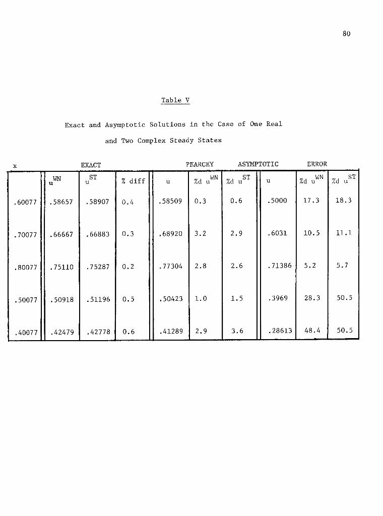
80
Table V
Exact and Asymptotic Solutions in the Case of One Real
and Two Complex Steady States
EXACT PEARCEY ASYMPTOTIC ERROR
WN u ST u % d i f f u /od u %d u u WN
%d u j ST %d u
.60077 .58657 .58907 0.4 .58509 0.3 0.6 .5000 17.3 18.3
.70077 .66667 .66883 0.3 .68920 3.2 2.9 .6031 10.5 11.1
.80077 .75110 .75287 0.2 .77304 2.8 2.6 .71386 5.2 5.7
.50077 .50918 .51196 0.5 .50423 1.0 1.5 .3969 28.3 50.5
.40077 .42479 .42778 0.6 .41289 2.9 3.6 .28613 48.4 50.5

81
23. Comparison of the theory with Monte Carlo Experiments
No exact solution of the two dimensional backward equation
(4.10), with b 1 given by (21.20,21) and ea^ given by (21.17),
could be found. Thus the asymptotic results w i l l be compared
with Monte Carlo experiments. The experiments were performed
by using the transition probabilities (21.7-10) or by working
with the Ito equation
dx = b(x)dt + /ea(i) dW , (23.1)
where W(t) is a standard Brownian motion process (Ito and
McKean, 1965). The two techniques lead to equivalent f i r s t
exit probabilities.
A) The Normal Case
When k = .038 and kx^ = .2225 in (21.5), the corresponding
deterministic system is the normal type. The f i r s t exit probability
was calculated using the theory of Chapter 2. The integration of
the equation for * n used a fourth order Runge-Kutta routine.
In Fig. 9 the deterministic phase portrait and the u = .3
contour of f i r s t exit probability are plotted. In Table VI the
probability calculated using the theory is compared with the
probability observed in Monte Carlo simulations.
The function *(x) was calculated in a v i c i n i t y of S by
a Taylor expansion. The contours were calculated by using the
leading part of the expansion of u(x) (eqn. 8.17).

82
Figure 9 Deterministic Phase Portrait and First Exit Boundaries in the Normal Case.' (Also shown is the u = 0.3 contour.)

Table VI
Comparison of the Theory with Monte Carlo
in the Normal Case
Test Point Theory
(.878, 1.025) .50
(.49, .058) .50
(.75, .75) .40
(.54, .55) .22
(.40, 1.24) .03
(.65, 1.125) .17
(.475, 1.20) .05
(.73, .72) .41
Experiments
Experiment (# tri a l s )
.51 (2000)
.49 (1700)
.39 (1750)
.23 (1500)
.02 (2000)
.15 (2000)
.04 (2000)
.39 (1700)

84
B) The Marginal Case
When k = .0533 and kx 1 = .24898 and the boundaries r
I, II are as shown in Fig. 10, the theory of Chapter 3 w i l l
apply.
The parameter in the Airy integral was calculated by the
method of characteristics, as described in §12. A double precision
Runge Kutta routine was used. When a ray hit the separatrix,
ty^_ = b 1 ^ = 0 . The intersection of the ray and the separatrix
was noted by calculating ty along the ray. Similar results
were obtained when a routine with error control was used
(UBC DDIFSY). The method of false position was used to calculate
iterates of a . The value of ty on boundary I was calculated
by a Taylor expansion about the node QQ, where ty =~—-/a^ .
In Table VII, we compare the theory with Monte Carlo experiments
for a number of test points. Also shown are some theoretical
results in which the Error integral was used. Using the leading
part of the asymptotic expansion, contours of f i r s t exit probability
could be calculated. The 0.30 contour is shown in Fig. 10. The
theory using the Error integral did not yield satisfactory results,
but the theory using the Airy integral did.
The Monte Carlo results are very sensitive to the location
of boundary I. Since the attractor QQ is within, the separatrix
tube, i t is possible to choose.boundary I so that the process
w i l l not hit I before II with probability close to 1. Thus, the Monte
Carlo study of marginal (and c r i t i c a l ) type systems is time

85
Figure 10 Deterministic Phase P o r t r a i t and F i r s t E x i t Boundaries i n the Marginal Case. (Also shown i s the u = 0.3 contour.)
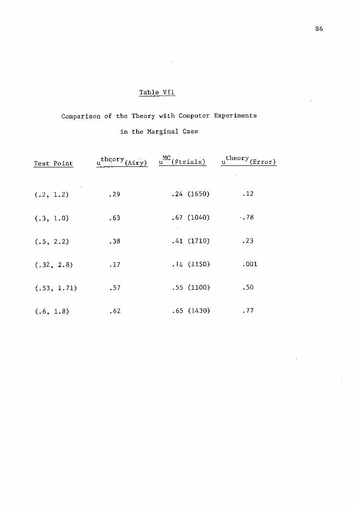
Table VII
Comparison of the Theory with Computer Experiments
in the Marginal Case
Test Point u t h e;° r y(Airy) u M C(#trials) u t h e° r y(Err
(.2, 1.2) .29 .24 (1650) .12
(.3, 1.0) .63 .67 (1040) -.78
(.5, 2.2) .38 .41 (1710) .23
(.32, 2.8) .17 .14 (1150) .001
(.53, 1.71) .57 .55 (1100) .50
(.6, 1.8) .62 .65 (1430) .77

consuming. On the other hand, the asymptotic calculations, although
sensitive to the location of the boundary, are not any more d i f f i c u l t
than in the normal case. In this sense, the Monte Carlo and
asymptotic techniques are complementary.
C) Marginal Bifurcation
When k = .069979 and kxj = .25901, the deterministic system
exhibits the marginal bifurcation (§10). In this case, the f i r s t
exit probability i s of l i t t l e interest (Fig. 11). The expected
time that i t takes the process to hit a specified curve R given
that x(0) = x, is of more interest. The function T(x) satisfies
equation (4.12). In Appendix C, we calculate the f i r s t term of
the asymptotic solution of (4.12). The solution is very similar
to the ansatz (11.2).
In Table VIII we compare the theoretical results with Monte
Carlo experiments. The theoretical results correspond to the
leading part of the asymptotic solution. Since the expected time
represents a f i r s t moment, the difference between the asymptotic
and Monte Carlo results for the expected time was larger than
for the probabilities.

Figure 11 Deterministic Phase Portrait at the Marginal Bifurcation. The Boundary R was used in the calculation of the mean f i r s t exit time.

89
Table VIII
Comparison of the Theory and Monte Carlo Experiments
in the Marginal Bifurcation
Test Point T(x) Theory T(x) Experiment (// Trials)
(.42, 2.06) 60.3 56.4 (950)
(.38, 2.36) 104.1 91.2 (400)
(.20, 2.0) 66.1 62.4 (2000)
(.3, 1.8) 37.7 35.0 (1550)
(.16, 2.4) 119.6 103.5 (400)
(.7, 2.2) 36.1 31.4 (1750)
(.6, 2.4) 74.9 68.2 (800)

90
D) The C r i t i c a l Case
When k= .08125 and kx^= .261199, and the boundaries I and II are r
as shown i n F i g . 12, the theory of Chapter 4 w i l l be applicable.
The parameters a,8 were calculated using the method of c h a r a c t e r i s t i c s ,
as described i n §17. A double p r e c i s i o n Runge-Kutta routine was used
to c a l c u l a t e the rays. More sophisticated routines, with error c o n t r o l ,
gave s i m i l a r r e s u l t s . Iterates of and 8Q were calculated using the
method of f a l s e p o s i t i o n . The values of ip on the boundaries I, II were
determined by Taylor expanding around the nodes and then following
rays that h i t the boundary. A s i m i l a r technique was used i n the mar
g i n a l case and at the c r i t i c a l b i f u r c a t i o n . The value of ij; i n a
v i c i n i t y of the separatrix was calculated by a Taylor expansion. The
de r i v a t i v e of * on S was calculated by integrating equation ( 1 8 . 1 ) .
A fourth order Runge Kutta routine was used. In Table IX, we compare
the Monte Carlo experiments and the t h e o r e t i c a l r e s u l t s .
The Monte Carlo r e s u l t s were very s e n s i t i v e to the l o c a t i o n of
the boundary. Since both a t t r a c t o r s P^ and P^ are contained by the
separatrix tube, i t i s possible to choose I and II so that the
p r o b a b i l i t y of h i t t i n g either boundary i s very small. The problem of
excessive machine time places a r e s t r i c t i o n on the choice of boundaries
I I , I I ; when the tube contains a stable steady state.

Figure 12 Deterministic Phase Portrait and First Exit Boundaries in the C r i t i c a l Case. (Also shown is the u = 0.6 contour).

Table IX
Comparison of Theory and Monte Carlo Experiments
in the C r i t i c a l Case
Test Point u t h e ° r y u^C(# trials)
(.7, 1.28) .67 .71 (2040)
(.5, 1.2) .63 .68 (980)
d.9, 2.0) .54 .50 (980)
(.6, 1.0) .76 .76 (1060)
(.5, .82) .78 .77 (1060)
(.9, 1.8) .59 .61 (980)

E) C r i t i c a l Bifurcation
When k = .0968493 and kx 1 = .1820033, the deterministic r
system exhibits the c r i t i c a l bifurcation. The theory of Chapter 4
and Appendix E applies. The calculation of ty was performed as
described in part D above.
In Table X we compare the theory of Chapter 4 with Monte Carlo
experiments. The widening of the boundary layer around S as the
type of deterministic system changes is clearly exhibited in
Figs. 9 and 13. In the normal case, the 0.3 contour is 0.93 units
from the saddle point. At the c r i t i c a l bifurcation, the 0.3 contour
is .275 units from the steady state.

94
Figure 13 Deterministic Phase Portrait and First Exit Boundary at the C r i t i c a l Bifurcation. (Also shown is the u = 0.3 contour.)

Table X
Comparison of the ' Theory with Monte Carlo Experiments
at the C r i t i c a l Bifurcation
Test Point u t h e ° r y u M C (# tri a l s )
(.4, 1.4) .46 .50 (1900)
C-6, 1.4) .54 .56 (1950)
(.6, 1.5) .50 .46 (1970)
(.8, 1.0) .87 .92 (2000)
(.3, 1.0) .68 .72 (2000)
(.5, 1.8) .29 .26 (2000)
(.2, 1.2) .54 .58 (1970)
(.7, 1.7) .44 .40 (2000)

Bibliography
Abramowitz, M. and I. Stegun (1965). Handbook of Mathematical Functions, Dover Publications, N.Y., N.Y.
Andronov, A.A., E.A. Leontovich, I.I. Gordon and A.G. Maier (1973). Qualitative Theory of Second Order Dynamic Systems. Halsted Press, N.Y.
Armstrong, C. (1975). Ionic pores, gates and gating currents. Quart. Rev. Biophysics 7(2): 179-210.
Arnold, L. (1974). Stochastic Differential Equations: Theory and Applications. Wiley-Interscience, N.Y.
Arnold, V.I. (1972). Lectures on bifurcations in versal families. Russian Math. Surveys 27(5): 54-123.
Barnett, V.D. (1962). The Monte Carlo solution of a competing species problem. Biometrics 18: 76-103.
Bartholomay, A. (1957). Stochastic models for chemical reactions. Bulletin Math. Biophysics 20: 97-118.
Bazekin, A.D. (1975). Structural and dynamic st a b i l i t y of model predator-prey systems. Institute of Animal Resource Ecology. Univ. of B.C., Vancouver.
Bleistein, N. and Handelsman, R. (1975). Asymptotic Expansion of Integrals. Holt, Rinehart and Wilson, N.Y.
Chang, M. and R.A. Schmitz (1975). Feedback control of unstable states i n a'laboratory reactor. Chemical Engineering Science 30: 837-846.
Chance, B. (1951). Enzyme substrate compounds, Advances in Enzymol 12: 153-190.
Cohen, D.S. (1972). Multiple solutions of-nonlinear partial differential equations. Springer Notes in Math., Vol. 322: 15-77.
Cohen, J.K. and R.M. Lewis (1967). A ray method for the asymptotic solution of the diffusion equation, J. Inst. Math. Appl. 3: 266-290.
Courant, R. (1962). Methods of Mathematical Physics, Wiley Inter-science, N.Y., N.Y.
Davis, H.T. (1962). Introduction to Nonlinear Differential and Integral Equations. Dover, N.Y., N.Y.

Degn, H. (1968). Bistability caused by substrate inhibition of peroxidase in an open reaction system. Nature 217: 1047-1050.
Delbruck, M. (1940). Statistical ifluctuations in an autocatalytic reaction. Jour. Chemical Physics 9: 120-124.
Dennis, J.E. and J.J. More (1977). Quasi-Newton methods, motivation and theory. SIAM Rev. 19(1): 46-89.
Feher, G. and M. Weissman (1973), Fluctuation spectroscopy. Proc. Nat. Acad. Sci. U.S.A. 70(3): 870-875.
Feller, W. (1952). The parabolic differential equations and the associated semi-groups of transformations. Annals of Math. 55(3): 468-519.
Feller, W. (1971). An Introduction to Probability Theory and Its Applications. Wiley Interscience, N.Y.
Frank, F.C. (1953). On spontaneous asymmetric synthesis, Bioch. Bioph. Acta 11: 459-463.
Gihman, I.I. and A.V. Skorohod (1972). Stochastic Differential Equations. Springer Verlag, New York.
Glansdorff, P.. and I. Pfigogine (1971). Thermodynamic Theory of Stability, Structure and Fluctuations. Wiley-Interscience, 1971.
Goldstein, J.C. and M.O. Scully (1973). Nonequilibrium properties of an Ising-model ferromagnet. Phys. Rev. B 7(3): 1084-1096.
Graham, R. (1974). Statistical theory of ins t a b i l i t i e s in stationary nonequilibrium systems with applications to lasers and nonlinear optics. Springer Tracts in Modern Physics, Vol. 66, Springer, Berlin.
G r i f f i t h s , R.B. C-Y Weng and J.S. Langer (1966). Relaxation times for metastable states in the mean-field model of a ferromagnet. Phys. Rev. 149: 301-305.
Harrison, L. (1973). Evolution of biochemical systems with specific c h i r a l i t i e s : a model involving t e r r i t o r i a l behavior. J. Theor. Biol. 39: 333-341.
Hartman, P. (1973). Ordinary Differential Equations, Hartman, Baltimore, 612 pp.
Heyde, CC. and E. Heyde (1971). Stochastic fluctuations in a one substrate one product enzyme system: are they ever relevant? J. Theor. Biol. 30: 395-404.

Higgins, J. (1967). Chemical oscillations. Indus. Eng. Chem. 59(5): 19-62.
Ito, K. and H.P. McKean (1965). Diffusion Processes and Their Sample Paths. Springer Verlag, 321 pp.
Keizer, J. (1975). Concentration fluctuations in chemical reactions. J. Chem. Phys. 63: 5037-5043.
Keller, J.B. (1958). A Geometrical theory of diffraction. Proc. Symp. Appl. Math. 8: 27-52.
Kubo, R., K. Matsuo and K. Kitahara, Fluctuation and relaxation of macrovariables, J. Stat. Phys. 9(1): 51-96.
Landau, L. and'E.M. Lifshitz (1968). Statistical Physics. Pergamon Pressj New York, N.Y.
Landau, L. and E.M. Lifschitz (1959). Fluid Mechanics. Addison-Wesley, Reading, Mass. 536 pp.
Landauer, R. and J.W.F. Woo (1972). The steady state far from equilibrium: phase changes and entropy, of fluctuations ; in Stati s t i c a l Mechanics, S.A. Rice et a l . , eds., Univ. of Chicago Press, Chicago, pg. 299-318.
Lavenda, B. (1975). Dynamic phase transitions in nonequilibrium processes. Phys. Rev. A 11(6): 2066-2078.
Lax, M. (1960). Fluctuations from the nonequilibrium steady state. Rev. Modern Phys. 32(1): 25-65.
Lax, M. (1966). Classical noise IV: Langevin methods. Rev. Mod. Phys. 38: 541-566.
Lecar, H. and R. Nossal (1971a). Theory of threshold fluctuations in nerves. I. Relationships between electrical noise and fluctuations in axon f i r i n g . Bioph. J. 11: 1048-1067.
Lecar, H. and R. Nossal (1971b). Theory of threshold fluctuations in nerves. II. Analysis of various sources of membrane noise. Bioph. J. 1068-1084.
Levinson, N. (1961). Transformation of an analytic function of several variables to a canonical form. Duke Math. J. 28: 345-353.
Levey, L. and L.B. Felsen (1969). On incomplete Airy functions and their application to diffraction problems. Radio Science 4: 959-969.

Ludwig, D. (1975). Persistence of dynamical systems under random perturbations. SIAM Rev. 17(4): 605-640.
Luneberg, R.K. (1945). Propagation of Electromagnetic waves. New York University, N.Y.
Lynn, R.Y.S. and J.B. Keller (1970). Uniform asymptotic solutions of second order linear ordinary differential equations with turning points. Comm. Pure. Appl. Math. 23: 379-408.
Ma, S.K. (1976). Scale transformations in dynamic'"models. Springer Lecture Notes in Physics, Vol. 54: 44-79.
Mangel, M. and D. Ludwig (1977). Probability of extinction in a stochastic competition. SIAM J. Appl. Math., 33:256-266
McQuarrie, D. (1967). Stochastic Approach to Chemical Kinetics, J. Appl.. Prob. 4: 473-478.
Matkowsky, B. and Z. Schuss (1977). The exit problem for randomly perturbed dynamical systems, 33:365-382
Matsuo, K. (1977). Relaxation mode analysis of nonlinear birth and death processes. J. Stat. Phys. 16(2): 169-195.
Moore, W. (1962). Physical Chemistry, 3rd edition. Prentice Hall, New York, N.Y.
Mori, H. (1965). Transport, collective motion and Brownian motion. Prog. Theor. Phys. 33(3): 423-455.
Nayfeh, A.H. (1973). Perturbation Methods. Wiley Interscience, New York, N.Y.
Nelson, E. (1967). Dynamical Theories of Brownian Motion. Princeton Univ. Press, Princeton N.Y.
Nitzan, A., P. Ortoleva, J. Deutch and J. Ross (1974). Fluctuations and transitions at chemical i n s t a b i l i t i e s : the analogy to phase transitions. J. Chem. Phys. 61(3): 1056-1074.
Olver, F.J.W. (1974). Introduction to Asymptotics and Special Functions. Academic Press, N.Y.
Papanicolaou, G.C. (1975). Asymptotic analysis of transport processes. Bull. Amer. Math. Soc. 81(2): 330-392.
Papanicolaou, G.C. and W. Kohler (1974). Asymptotic theory of mixing stochastic ordinary differential equations. Comm. Pure Appl. Math. 27: 641-668.

Pearcey, T. (1946). The structure of an electromagnetic f i e l d in the neighborhood of a cusp of a caustic. Phil. Mag. 37: 311-317.
Perlmutter, D.D. (1972). Stability of Chemical Reactors. Prentice-Hall, Englewood C l i f f s , N.Y.
Pincock, R.E., R.R. Perkins, A.S. Ma and K.R. Wilson (1971). Probability distribution of enantiomorphous forms in spontaneous generation of optically active substances. Science 174: 1018-1020.
j
Schuss, Z. (1977),. Stochastic Differential Equations. Notes, University of Delaware.
Sinai, Ya. G. (1970). Dynamical systems with elastic reflections. Russ. Math. Surveys 25: 137-189.
Singer, K. (1953). Application of the theory of stochastic processes to the study of irreproducible chemical reactions and nucleation processes. J. Ray Stat. Soc. B 15: 92-106.
Stein, W.D. (1967). The Movement of Molecules across Cell Membranes. Academic Press, New York.
Van Kampen, N.G. (1976). The expansion of the master equation, Adv. Chem. Phys. 34: 245-309.
Ventcel, A.D. and M.I. Freidlin (1970). On small random perturbations of dynamical systems. Russ. Math. Surveys 25: 1-55.
Vereen, A.A. and L.J. DeFelice (1974). Membrane noise Prog. Bioph. Mol. Biol. 28: 191-265.
White, A, P. Handler and E.L. Smith (1968). Principles of Biochemistry, 4th edition, McGraw H i l l , N.Y.
Williams, R.G. (1977). The Stochastic Exit Problem for Dynamical Systems. Thesis, California Institute of Technology.
Wong, E. and M. Zakai (1965). On the relation between ordinary and stochastic differential equations. Int. J. Eng. Sci. 3: 213-229.

Appendices
With the exception of Appendix C, these appendices are concerned
with the treatment of some fine points related to the asymptotic
expansions given in the body of the paper. In Appendix C, we show
how to construct the leading term in the solution of the equation
for the mean exit time (4.12).
Appendix A: Solution of the I n i t i a l Value Problem for h^
In Chapters 2-4, a characteristic i n i t i a l value problem arises.
The function h^ satisfies
In equation (A.l), F(x) is bounded, integrable and differentiable. 2 3
The function f(ty) = -ty, -(ty ~^Q) > or ty - a^ty - g^ in the normal,
marginal and c r i t i c a l cases respectively. Except at the bifurcations
f(ty) vanishes on the separatrix but f * (ip) does not. At the
marginal bifurcation f and f 1 vanish on the separatrix, but f"
does not vanish. At the c r i t i c a l bifurcation, , f, f 1 and f"
vanish, but f 1 1 1 does not vanish. To avoid repetition, we shall
not consider either of the bifurcations. On the separatrix, equation
(A.l) becomes
- a -ity.ty.f'ity) - a Jh.ty.f(ty) • 1 J i J
+ c^tyA^f (ty) = F(x) . (A.l)
0 a 2 (tys) = F(x(t)) , (A.2)

102
where * g i s the value of * on the s e p a r a t r i x . Since d/dt =
b^d/dx*~, at the saddle p o i n t , P^,dh^/dt vanishes . Equation (A.2)
i s then solved for h^(P^) . Once h^ i s known at the saddle ,
equation (A.2) can be solved to obtain h^ on the s e p a r a t r i x . We
denote t h i s s o l u t i o n by h^ . s
0 ' The i n i t i a l value problem P : {solve ( A . l ) with h = h on S}
s
i s a c h a r a c t e r i s t i c i n i t i a l value problem (Courant, 1962) s ince the
s eparatr ix S corresponds to the d i r e c t i o n of d i f f e r e n t i a t i o n i n
( A . l ) . The problem P i s not a t y p i c a l c h a r a c t e r i s t i c i n i t i a l value
problem; i t i s more s ingu lar (see a l so Appendix F , where we give an
existence proof for these types of equat ions) . The presence of the
s i n g u l a r i t y on the i n i t i a l manifold allows the unique determination
of h^(x) . We construct a new manifold S ' , which w i l l
not be a c h a r a c t e r i s t i c mani fo ld . Let v_ = Dh/Sx 1 . If ( A . l ) i s
d i f f e r e n t i a t e d with respect to x"*" and evaluated on the s e p a r a t r i x ,
we obta in
d v l F + a \ = V ( A - 3 )
where
a 1 = b 1 ^ + ^ ^ j f ' ( * s ) - a % il^f'Ol^) (A.4)
a 2 = b 2
5 ; L - a 2 j i | ; ' 0Pg) (A. 5)
Y = F - hV 1 3 Y.iJ;,f'W + c 1 * . f ( * ) ] , 1 . (A.6) i 1 J- 2 J •L
2
D i f f e r e n t i a t i o n of ( A . l ) with respect to x and evaluat ion on
the separatr ix y i e l d s :

d v 2 i i r + 6 v . = Y 2 (A.7)
where
B 1 = b 1 ^ - a ^ ^ f ' ( < P g ) (A.8 )
g 2 = b 2 ' 2 + T " ' ^ j V ' ^ ( A - 9 )
Y 2 = F, 2 - h°[.aljT|; ifr f ' ( » ) + c ^ . f O p ) ] , . (A.10)
At the saddle point, P^, equations (A.3, 7) become
a 1v1 + a 2 v 2 = Y 1(P ]_) (A. 11)
8 Lv1 + B 2v 2 = Y 2 ( P 1 ) • (A.12)
Equations (A.11, 12) determine the in t e g r a t i o n constants when
(A.3, 7) are solved. Once v ^ O ^ ) a r e known, v^>v2 c a n b e
determined along the e n t i r e separatrix.
The new manifold S' i s determined by a Taylor expansion about
tr(x ,) = h°(x ) + v.(x ) ( x 1 , - x 1 ) + 0((x ,-x ) 2 ) . (A.13), s' S 1 s s s s s
The value of h^ on S' i s not a r b i t r a r y , but i s s p e c i f i e d by
equation (A.13). In (A.13), x i s a point on S; x , i s a s s
point on S' . We are free to choose the manifold i n any form
desired. In p a r t i c u l a r , S' can be chosen so that i t i s nowhere
tangent to deterministic t r a j e c t o r i e s . The problem P': {Solve (A.l)
with i n i t i a l data h^ = h^, on 5'} i s a well posed problem that
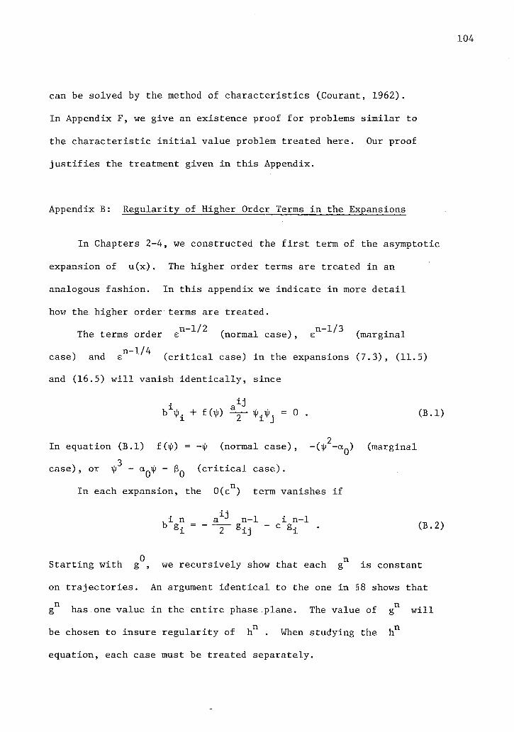
can be solved by the method of characteristics (Courant, 1962).
In Appendix F, we give an existence proof for problems similar to
the characteristic i n i t i a l value problem treated here. Our proof
j u s t i f i e s the treatment given in this Appendix.
Appendix B: Regularity of Higher Order Terms in the Expansions
In Chapters 2-4, we constructed the f i r s t term of the asymptotic
expansion of u(x). The higher order terms are treated in an
analogous fashion. In this appendix we indicate in more detail
how the higher order terms are treated.
The terms order e n (normal case), e11 (marginal
case) and e11 ( c r i t i c a l case) in the expansions (7.3), (11.5)
and (16.5) w i l l vanish identically, since
i a ± j
b *. + f (*) ^— ^ = 0 . (B.l)
2 In equation (B.l) f (ip) = -* (normal case), - ( * -01Q) (marginal
3 case) , or i() - a^> - BQ ( c r i t i c a l case).
In each expansion, the 0(e n) term vanishes i f
i j -i - i , l n a n-1 l n-1 „. b g i = " — g ± J - c g ± . (B.2)
0 n Starting with g , we recursively show that each g is constant
on trajectories. An argument identical to the one in §8 shows that
g n has one value in the entire phase,plane. The value of g n w i l l
be chosen to insure regularity of h n . When studying the h 1 1
equation, each case must be treated separately.

105
1) Normal Case
The 0(e n +^ / ,' 2) term in (7.3) vanishes i f
i j b V - a1Jh?i|/.i|i - hn{ (#.).} - c\.b.nty x i j 2 Tx j l
(B.3) a n, _ a , n-1 n l , x, n-1
= x— g ty. . —Tr- h. . - g c i - c h. 2 xj 2 xj x x
n n—1
The functions g , h are assumed to be known. On the separatrix
(B.3) becomes
,,n i j i j i j -. . . -dh a ,n, , a n , _ a , n-1 n x, x, n-1 .. -jz T~ " ty -ty • = o § ty - • n - • - % c ty. - c h. . (B.4) dt 2 l j 2 xj 2 xj x x
In equation (B.4), d/dt = b19/9x"L vanishes at the saddle point.
We choose g n so that hn w i l l vanish at the saddle point. Once
g n is known, equation (B.4) can be used to determine h n on the
separatrix. Once h n is known on the separatrix, i t can be calculated
everywhere in the phase plane using the technique described in
Appendix A. 2) Marginal Case
n*4*2 / 3 The 0(e ) term in (11.5) vanishes i f
i j o • • i j i j i , x, n , n a J r , ,. 2 N 1 . i j n . , a J n, , a J , n-1 b h. - h — [ty±(ty -a Q)] . + a Jg.^. + — g ty±. + — h..
.,2 w i j , n , . i , n - l i n , - (ty - a J (a h^ipj) + c h i + c g ty^
i , ,n,,2 N ,nv"^ , , / n+l-k ,,2 ., n+l-k, .„ - c ij^h (ty -a ) + I — ty^.ig - (ty -a )h (B.5)
k=l J
n+1 „ i j n , • + I a k [ h n + 1 k ( b % . - (ty-aQ)^- ty±ty )] + j; c ^ . a k h n - k
k=l J k=l i j n+1 ty.ty. iin k-1 n , . Z k=2 Z j=l J k J k=l k 1 2 1 J
= 0 .
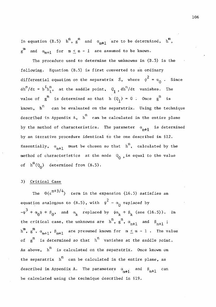
106
In equation (B.5) h n, g n and an + ± a r e t o be determined, h m,
g™ and c^+i for m <_ n - 1 are assumed to be known.
The procedure used to determine the unknowns in (B.5) is the
following. Equation (B.5) is f i r s t converted to an ordinary 2
differential equation on the separatrix S, where = . Since
dh n/dt = b 1!^, at the saddle point, Q" } dh n/dt vanishes. The
value of g n is determined so that h (Q-^) = 0 . Once g n is
known, h n can be evaluated on the separatrix. Using the technique n
described in Appendix A, h can be calculated in the entire plane
by the method of characteristics. The parameter an + ^ i s determined
by an iterative procedure identical to the one described in §12.
Essentially, an + ^ must be chosen so that h n, calculated by the
method of characteristics at the node QQ } i s equal to the value of h n(Q ) determined from (B.5)
3) C r i t i c a l Case
The 0 ( e n + 3 ^ 4 ) term in the expansion (16.5) satisfies an 2
equation analogous to (B.5), with ~ aQ replaced by 3
-lp + a ^ i + BQ, and replaced by ifa^ + B . (see (16.5)). In the c r i t i c a l case, the unknowns are h n, g n, a and B ., ;
n+1 n+1 h m, s m, a , 8 .-, are presumed known for m < n - 1 . The value ° m+1 m+1 — of g n is determined so that hn vanishes at the saddle point.
As above, h 1 1 is calculated on the separatrix. Once known on
the separatrix h n can be calculated in the entire plane, as
described in Appendix A. The parameters a and B ,-, can n+1 n+1
be calculated using the technique described in §19.

107
The above procedures insure that the higher order terms in the
asymptotic solutions are regular and bounded.
Appendix C: Asymptotic Solution of the Expected Time Equation
Let T(x) be defined by
T(x) = E{t: x ( t ) £ . R , x(t ' ) £ . R t' < t|x(0) = x, x(t) hits R } . ( C l )
Then T(x) is the expected amount of time i t takes the process to
hit R starting at x . In §4, we showed that T(x) satisfies
the backward equation
• ^ f — T. . + b ^ . + e c V = -u(x)',. (C.2)
In (C.2), u(x) is the probability of eventually reaching R ,
conditioned on x(0) = x . Equation (C.2) is an inhomogeneous
backward equation. In this appendix, we give the asymptotic
solution of (C.2). The solutions are closely related to the
solutions in Chapters 2-4, so that only the f i r s t term w i l l be
considered. Equation (C.2) must be supplemented by boundary
conditions. Let d be the distance from x to R .
The f i r s t boundary condition is
T(x) E 0 x £ R . (C.3)
As a second boundary condition, we require that T(x) is bounded
as jd| —> °° . In Feller's terminology (Feller, 1952), we are
requiring that °° is an "entrance boundary". Feller's theory

108
applies to one dimensional systems and there is no analogous two
dimensional theory. On the other hand, the second boundary condition
is in accord with intuition for the systems of interest here.
C l Normal Case
The results presented in Chapter 2 and the asymptotic analysis
of a one dimensional version of (C.2) indicate that a possible
solution of (C.2) i s
T(x) = I e ng n F 0 K x ) / ^ ) + e n + 1 / 2h n(x)F'(*(x)// £")
n n ( C' 4 )
+ En k n(x) .
In (C.4), g n(x), h n(x), k n(x) and *(x) are to be determined.
The function F(z) satisfies
2 dz 0 — — 1
dz
Equation (C.5) is an inhomogeneous version of the equation that
the Error integral satisfies.
When derivatives are evaluated, (C.5) is used to replace F"
by (-ipF1//! - 1). After substitution into equation (C-2), terms
are collected according to powers of e . The leading term (n=0)
vanishes i f the following equations are satisfied: i a i j
0(F.7/e): b i|)± - — = 0 ( C- 6)
0(F): b±g°± = 0 (C.7)
0(e°): b i k ° i - ^ g° = -u(x) (6.8)

109
O(A'): bV + V- gV • " ^ . a ^ t y . t y - b ° c \ . t y (C.9)
+ g°c\ - h° -^-[(W.) .] = 0 .
Equations (C.6, C.7, C.9) are identical to equations (7..4-6 ).
Thus, the constructions in §8, 9 for ty and h^ are applicable
here. Equation (C.7) indicates that is constant on trajectories.
The argument in §8 shows that g^ has the same value on a l l
trajectories.
At the saddle point P^, b(x) vanishes. Equation (C.8)
becomes
-a 1 J ... ... 0 2~ = -uCPJ . (CIO)
Thus, the value of g^ is g^ = 2u(P^) /a^ty^ty . Once g^ is
known, k^ can be calculated by the method of characteristics i f
i n i t i a l data are given. We assume that R is not a characteristic
curve, and set k^ = 0 on R . (If R is a characteristic curve,
then the equation (C.8) must be treated by a procedure similar to
the one described in Appendix A).
We also assume, without losing generality, that ty = ty^ on
R . Then, we set z Q = tyQ//e and ¥(ty //e) = F'(i|; //e) = 0 in
equation (C..4). With the above choices, T(x) = 0 i f x €. R •
If R is not a level curve of ty, then T(x) w i l l not identically
vanish i f x £ R but w i l l be exponentially small (§8.2).
C.2. Marginal Case
The above solution for T(x) breaks down in the marginal case
for the same reason that the solution for u(x) that used the Error

110
integral broke down (§11.1). Based on the ansatz given in §11 and
the expansion of a simpler problem, we seek a solution of (C.2) of
the form
T(x) = I £n g n ( x ) B ( * / e 1 / 3 , a/e 2 / 3, 1/ £
1 / 3, y)
+ e n + 2 / 3 h n ( x ) B ' ( 1 p / £1 / 3 , a/e 2 / 3, 1/ £
1 / 3, y) (C.ll)
'+ e nk n(x).
In ( C . l l ) , the function B,(z, a, y^, y^) satisfies an inhomogeneous
version of the equation that the Airy integral satisfies:
2 d B(z;a,y 1Y 2) 2 d B
~2 = - ( Z -a) — - Y l + y 2 z zQ±z. (C.12) dz
When derivatives of T(x) are calculated, (C.12) is used to replace
B" by terms involving B', ip, a and y . We assume that
a = _ c^.ek and y = _ Y^e^ • (C.13)
After derivatives of T(x) are calculated and substituted into
equation (C.2), terms are collected according to powers of e . The
leading term (n=0) vanish i f
0(e 1 / 3B'): b 1 ^ - ^ (*2-aQ) = 0 (C.14)
0(e°B): b i g ° i = 0 (C.15)
0(e°): b i k ° ± + * i * j g 0 ( - l + i p Y 0 ) = -u(x) . (C.16)
2/3 0 The 0(e B 1) term vanishes i f h satisfies equation (11.8).

I l l
Equation (C.14) is identical to 0-1.6). Thus, the constructions
for i p , 01Q and h^ in §12-14 can be used here. Equation (C.15)
indicates that i s a constant on trajectories. The argument
used in §8.2 shows that g^ has the same value on a l l trajectories.
In the marginal case, the vector f i e l d b(x) vanishes af'two
points QQ, within the domain of interest. At these two points,
equation (C.16) becomes
a 1 J i P i p . 0
2 3 g ("1 + ^YQ) = -u(Qk) k = 1,2 . (C.17)
Equation (C.17) provides two equations for g^ and YQ • At the
marginal bifurcation, an application of 1'Hospital's rule shows
that YQ = 0 • Equation (C.17) s t i l l provides one equation (at the
saddle-node Q) for g^:
- a ^ i P . i P 0
o g = -u(Q) . (C.18) Q
Once g^ and YQ are known, k^ can be calculated as described
abovef
We also assume that R is a level curve of i p , say i p = i p ^
on R . Then, in (C.12) we set z Q = t p Q / e ' and B(z Q) = B'(z Q) = 0.
With these choices, T(x) = 0 on R .
If R is a characteristic curve, or i p is not constant on
R, the remarks of the previous section apply.

112
C.3. C r i t i c a l Case
The solution in the previous section w i l l break down i f the
domain of interest contains three steady states or the deterministic
system exhibits the c r i t i c a l bifurcation (§15, 16.1). Based on
the results in §16.2 and the expansion of a simpler problem, we
seek a solution of (C.2) of the form
T(x) = I en g n ( x ) Q ( * / £
1 / 4 ; a/e1/2, 6/s 3 / 4, l / e 1 / 2 , - y ^ ^ 4 , yj
+ en + 3 /V(x)Q' ( (p/ £
1 / 4; a/e 1 / 2, 3/ £3 /\ 1/, U\ ^ / e 1 ' 4 , Y 2 >
+ e I 1k n(x). (C.19)
In (C.19), the function Q(z;a, g,Y^,Y2 3 ) satisfies
2 = ( z 3 - a z - e ) | ^ - Y l + Y 2z + Y 3 z 2 z
0 1 2 ' ( C - 2 0 )
dz
When derivatives of T(x) are evaluated, (C.20) is used to replace
Q" by terms involving Q1 , a,$,y^ and y^ . After derivatives are
evaluated and substituted into (C.2), terms are collected according
to powers of e . We assume that
a = I <\ e k 6 • = I B ke k
Y l = % Y l k e k y2= I Y 2 k e k • (C.21)
The f i r s t term of the asymptotic solution vanishes i f
0(e~1/UQ'): b 1*. + ^.^ (*3-aQiJ;-B0) = 0 (C.22)

113
0(e°Q): b 1 g ° i = 0 (C.23)
0(e°): b ^ 0 . + g°(-l + Y10I|«. + Y 2 Q^ 2) 2 1 j = -u(x). (C.24)
The CKe^^Q') term vanishes i f h^ satisfies equation (16.8):.
Equation (C.22) is identical to (16.6). Thus, the constructions
given in §16-19 for ty, a^, BQ and h^ are applicable here.
At the nodes PQ, P 2 and saddle point P^, b(x) vanishes.
Equation (C.24) becomes
' l O ^ k ' ' '20r V i k y / 1 " V ik g°(-l + Ynn<Kpv> + Y 9 n ^ 2 ( P 1 . ) ) a o ^ J = -u(Pj k = 0,1,2 . (C.25)
The constants g^, Y- Q and Y 2Q c a n be determined from (C.25).
Once g^, Y-J Q and Y 2Q a r e known, k*"* can be determined as
described in §C.l. At the c r i t i c a l bifurcation Y- Q = Y 2Q = 0 •
We assume that R is a level curve of ty, ty = ty^ on R . Then,
in C.20, we set z Q = ty^e1^ and Q(z Q) = Q'(ZQ) = 0 . If
k° = 0 on R , then T (x) = 0 on R .
Appendix D: Regularity at the Marginal Bifurcation
In Chapter 3, the asymptotic solution of the backward equation
was constructed assuming that two steady states, and Q^,
were contained by the separatrix tube. As a deterministic parameter
n varies, the two steady states move together and coalesce at
n = 0 . The marginal type dynamical system was defined by intro-1 2 1
ducing new coordinates y (n)» y (n), where y (n) was defined in the direction of the eigenvector of"the non-negative eigenvalue at 0^.

The deterministic system i s
y = b(.y,n) (D.l)
The steady state Q is of the marginal type i f
a) det(b^(Q ,0)) = 0
b) (Q,0) = 0
c)
d)
b 2 , 2 . ( Q , 0 ) + 0
b '11 b '11 t 0.
(D.2)
The conditions (D.2) were introduced in §11 and have the following
interpretations. Condition a) indicates that B = (b 1, ) has a
zero eigenvalue when n = 0 . Condition c) insures that the second
eigenvalue of B is non-zero. Condition b) indicates that the
linear dynamics in the y"*" direction vanish and d) indicates
that the dynamics in the y"*" direction are quadratic. When n = 0,
the double point QQ/Q-J i s called a saddle-node (Andronov et. a l .
(1973)). In this Appendix, we show that the constructions of
Chapter 3 are regular at the marginal bifurcation. This demonstration
consists of three parts: 1) F i r s t , we show that 9a/3n ^ 0 when
n = 0 . Our technique can be used to calculate a power series
a = JA.T]X for a in terms of the deterministic parameter.
2) Second, we show how to calculate the normal derivative of ty
on the separatrix, at the marginal bifurcation. 3) Third, we
show that h^ can be calculated at the marginal bifurcation.

D.l. Regularity of a
In §11, we showed that
, i , a ± j
b iii. — 1 2 ^ (i|> -a Q) = 0 . (D.3)
Also, *(QQ) = -/a Q and ) = /a Q When QQ and coalesce,
a,Q must vanish. When equation (D.3) is differentiated with respect
to n and evaluated at (k=l,2), we obtain
b V i a1Ji|j.ip.
l i l l (D.4)
When 9ip/8ri is eliminated from the two equations (D.4), and the
limit ri —> 0 is taken, we obtain
3 a0 - 2 b 'n*i'Q , = ij i a t 71 = 0 (D.5)
In order to expli c i t l y calculate 9a/9n, the must be known at
the saddle node Q . The derivatives of * are calculated in §D.2.
The higher derivatives of a with respect to n can be calculated
in an identical fashion. Equation D.3 is differentiated twice
with respect to n and evaluated at QQ and 0^:
b 1, nn I
+ 2b , <JJ. , n in i - l (2* 2 - 2*(v*nll - rf°)
Qk 9n
= 0 (D.6)
From (D.4). g*/9n and 9if^/9Ti can be expressed in terms of da^/dri

116
Thus, the ty term can be eliminated from(D.6)and i t is possible nn •
2 2 to calculate 3 a^/Sri . This procedure can be repeated r times
r
i f the deterministic equations are C with respect to n • In
this fashion, we can construct a truncated power series, of order
r, for O(Q in terms of n . Such power series are useful when
the deterministic equations have complex steady states (§20). D.2. Calculation of the Normal Derivative of ty
The easiest way to show that ty can be calculated on the n
1 2
separatrix when ri = 0 is to use the (y ,y ) coordinate system
and the variational equations analogous to (8.6). These are, when n = 0
dty - j - ^ + b1,. ty. = 0 on S k = 1,2 . (D.7) dt k I
At the saddle node b(x) vanishes, so that (D.7) becomes
b 1 , k ^ i =0 k = 1,2 . (D.8)
The condition for a nontrivial solution of (D.8) is that det(b 1, ) = 0, K.
condition (D.2a). If 3ip/3y'x can be calculated, then the normal
derivative of ij; can be evaluated. In the y variables, when
n = 0, equation (11.6) is
~ i U L _ a « ty2 = o . (D.9) x 2 l 1 By1 z dy1 3yJ
When equation (D.9) is differentiated with respect to y"*~ and
evaluated at the saddle-node, we obtain

117
b 1,. = 0, (D.10)
dy
which is satisfied identically due to condition (D.2b). When (D.9)
is differentiated twice with respect to y^ and evaluated at the
saddle-node, we obtain (using conditions(D.2))
3y 9y 3yJ 3y
Using the fact that the tangential derivative of \b vanishes on 2 1 the separatrix, 3*/3y can be expressed in terms of 3ip/3y
Then (D .11) becomes an algebraic equation for dib/dyX . We obtain
_3jj_ =
3 y 1 _
b '11 " b '11 11 12 . 22 a - za + a
4 0 at n = 0 . (D.12)
Since (a ) is positive definite on S, equation (D.12) is always
meaningful.
Since the f i r s t derivatives of ij; can be calculated at the
saddle-node, the derivatives can be calculated along the entire
separatrix by solving (D.7). Hence, the normal derivative of ib
can be calculated along the entire separatrix.
D.3. Calculation of h^ at the Bifurcation
When n and vanish, equation (11.8) becomes
.i.0 h° i j . . , ,2. . ,2 ij.O. . a 1 J , , 0,2 b h ± - y- a J (dy ) ) - * a J h ip± + a± — ib±ib^ ib
i j , i j , , (D.13) a *. . n • A • n o a ii.ib. n r i i 0 x, 0 x 0,2 r x r i 0 + — 5 — ^ g + c ip.g + c ip.h ib - a n r — g = 0 .
On the separatrix, where ib = 0, equation (D.13) becomes

„ 0 a 1 J^.. + 2cXty. - a^aX2ib.ty.
g - = -C U ~ ^ L ) S ° = H(x) .. (D.14)
We choose so that the right hand side of (D.14) vanishes at the
saddle-node. In order to calculate the value of h^ at the saddle-node
•we, differentiate (D.13) with respect to x and evaluate the
result at the saddle-node. We obtain
A n • • a±2ib. . . a±2ty .ib. _ _x ,0 ,0 xj r , , , •. T x j 1. , i I N 0 b , kh. - h a " ( " ~2 - ^ ± + a l —2 \ k g
k = 1,2 . (D.15)
Condition (D.2a) (det(b 1, ) = 0) allows the elimination of the
derivatives of h^ from (D.15). When the resulting expression
is solved for h^, we obtain
0 - ( b \ 2 + b 2, 2)!T, + ( b 1 ^ + b 2, 1)H, 2
h (Q) 1 —2 1 2 a Jty±ty^[b , 2 + b , 2 - b , ± - b ,1H>1
(D.16)
In (D.16), H(x) is the right hand side of (D.14). On the separatrix,
o H(x(s))ds . (D.17) h°(t)
t
Once h^ is known on the separatrix, the technique of Appendix A
can be used to calculate' everywhere in the plane.
Appendix E: Regularity at the C r i t i c a l Bifurcation
In Chapter 4, the asymptotic solution of the backward equation
was constructed assuming that three steady states P n, P^ and P 2
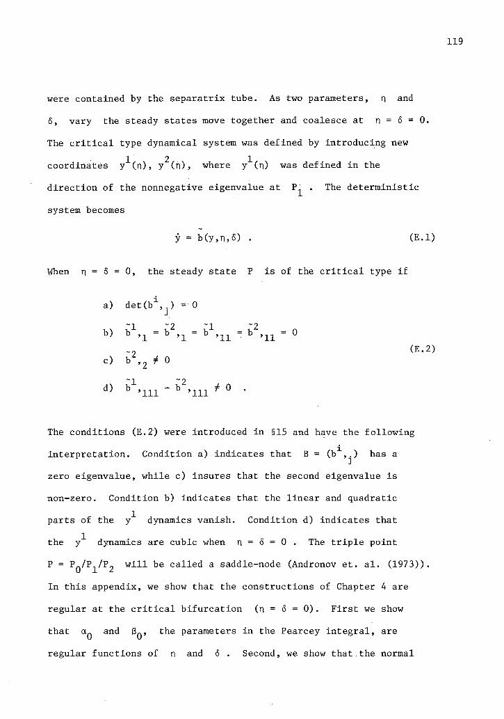
119
were contained by the separatrix tube. As two parameters, n and
6, vary the steady states move together and coalesce at ri = 6 = 0.
The c r i t i c a l type dynamical system was defined by introducing new 1 2 1 coordinates y (n) , y (n), where y (n) was defined in the
direction of the nonnegative eigenvalue at P^ . The deterministic
system becomes
y = b(y,n,6) . (E.l)
When n = 6 = 0, the steady state P is of the c r i t i c a l type i f
a) d e t C b 1 , ) = 0
b) b 1 ^ = l2,x = b \ 1 ; L = b 2 , l x = 0 ~ ? (E.2)
c) b Z , 2 * 0
d) b 1 , m - b 2 , m # 0 .
The conditions (E.2) were introduced in §15 and have the following
interpretation. Condition a) indicates that B = (b 1,^) has a
zero eigenvalue, while c) insures that the second eigenvalue i s
non-zero. Condition b) indicates that the linear and quadratic
parts of the y 1 dynamics vanish. Condition d) indicates that
the y X dynamics are cubic when n = 6 = 0 . The tri p l e point
P = P Q/P 1/P 2 w i l l be called a saddle-node (Andronov et. a l . (1973))
In this appendix, we show that the constructions of Chapter 4 are
regular at the c r i t i c a l bifurcation (n = <5 = 0). First we show
that a n and BQ, the parameters in the Pearcey integral, are
regular functions of r\ and 6 . Second, we show that the normal

120
derivative of tp can be calculated at the c r i t i c a l bifurcation.
Third, we show that h^ can be calculated at the c r i t i c a l bifurcation.
'Our arguments are analogous to those of Appendix D.
E. l . Regularity of a n and BQ
In §16 we showed that
i j o
b 1*. + OP -C^-BQ) = 0 (E.3)
and that ^(P^) = ^ = 0>1>2> where ^ are the ordered roots
of 3
ip - aQib - BQ = 0 .
When PQ,P^,P2 coalesce, and BQ must vanish and ip(P) = 0 .
We shall calculate the derivatives of 01Q and BQ with respect
to n; the calculation of derivatives with respect to 6 uses an
identical procedure. The procedure used is a generalization of the
procedure in §D.l.
When (E.3) is differentiated with respect to n and evaluated
at P , we obtain
b 1, n l Pk 2
13'" • 2 3 a0 8 30 v (+3ip, ip - a . i p - ip -r-V- - = 0 p , k n O n n 3 n 3n k
a J i p . i p . + l i - l
k = 0,1,2 . (E.4)
As in §D.l, ip and 3a „ / 8 n are eliminated from the three equations ri 0 generated by (E.4). The limit n —> 0,6 —> 0 is taken to obtain
9BQ a 1 , ^
i 3 (E.5)

121
The , values of ty at the steady state P are needed to calculate
3BQ/3TI . These derivatives are calculated in §E.2. The second and
higher (up to order r i f the deterministic equations are C in
n) derivatives of 8 n can be calculated in an analogous fashion
(§D.l).
In order to obtain a power series for in terms of n and
6, equation (E.3) is f i r s t differentiated with respect to x , then
n . The resulting system of equations is solved for da^/dr] . When
the limit n —>• 0, 6 0 is taken we obtain
3a n 2 D 1 > I ty. 0 _ y 'kri x
k a J ty . ty. ip, (E.6)
The higher derivatives of a n with respect to n can be calculated
in a similar fashion.
By using these techniques, we can generate power series
« 0 = I A i j n i 6 J e 0 = ^ ' ( E - 7 )
These power series are useful when the deterministic system has
two complex steady states with small imaginary part (§20).
E.2. Calculation of the Normal Derivative of ty
At the c r i t i c a l bifurcation, the equation for the derivatives
of ty on the separatrix i s
dty, dt + ^ ' k ^ i = ° k = 1,2 . (E.8)

122
At the steady state P, (E.8) becomes
b , k * ± = 0 k = 1,2 (E.9)
These equations w i l l have a nontrivial solution (condition E.2a)
In the y variables, equation (E.3) is (at n = 6 = 0)
~ i M _ a * ( 3 =
2 . i „ j r /
9y 9y 9y (E.10)
When (E.10) i s differentiated three times with respect to y
evaluated at P and simplified using (E.2a-d) we obtain:
'111 i i i 1 ;
9y 9y 9yJ 9y (E.ll)
An argument identical to the one in §D.2 leads to
9*
9yJ
' ~1 ~2 _ ( b '111 " b
11 _ 12 22 |a - 2a + a
1/4 (E.12)
Once the derivatives of * are known at P, they can be calculated
along the entire separatrix using equation (E.8). Thus, the normal
derivative of * can be calculated on the separatrix.
E.3. Calculation of h 0
The technique used to calculate h^ i s analogous to the one in
§D.3. Equation (16.10) i s f i r s t evaluated on the separatrix. The
parameter vanishes and is chosen so that h^ is regular
at P . Equation (1.6.10) is differentiated twice and evaluated at

123
P, in order to calculate h^(P) . Once h^(P) is known, can
be calculated along the entire separatrix. The technique of
Appendix A can then be used to calculate h^ in the entire plane.
Appendix F: Existence of Solutions of the General Eikonal Equation
In this appendix, we prove the existence of solutions of the
equation
1 2 • i j , F(x ,x ,ty,ty±,ty2) = b 1^. - ty ty±ty. = 0 (F.l)
with i n i t i a l data ty = 0 on the separatrix S . Equation (F.l)
arises in the normal case. The marginal and c r i t i c a l cases are treated
in a similar fashion, although some details are changed.
Associated with equation (F.l) is a system of ordinary differential
equations (Courant, 1962). Let p_ = ty . The characteristic or ray
equations are
dx 1 , i . i j — = b - tya Jp.
ds l ds
dp, . a1-1, d i " = _ b ' k P i + — + a P i P j P k k = X ' 2
Integrating equations (F.2) is equivalent to solving (F.l). The
i n i t i a l value problem for (F.l) with i n i t i a l data on the separatrix
is a characteristic i n i t i a l value problem. Namely, the i n i t i a l data
are given on a curve that is a solution of (F.2). In general, a

124
characteristic i n i t i a l value problem does not have a unique solution
because i t is not possible to calculate * on the i n i t i a l manifold. r n
In this problem, the i n i t i a l manifold is more singular than usual,
since i t contains the saddle point. Also, F ^ vanishes
at the singularity. These singularities distinguish
our problem from the usual characteristic i n i t i a l value problem and
allowed the calculation of * on the i n i t i a l manifold. This n
calculation was given in Chapter 2. Since we are able to calculate \ b on the i n i t i a l manifold, this characteristic i n i t i a l value problem n has a unique solution.
Let N denote distance normal to the separatrix and Y measure
distance along the separatrix, with the saddle point representing
Y = 0 . The separatrix corresponds to N = 0 . When equations (F.2)
are rewritten in terms of (N,Y) we obtain (using a Taylor expansion)
f i = N - *a l jp. + 0(N2+Y2) ds j
^ =-Y - *a 1 Jp. + 0(N2+Y2) (F.3) ds j
d* 1 , i j -r 3 1 = - - 0-*a Jp.p. ds 2 i J d p
k _± , a'k ds b ' k P i + — P i V + a 1 J p i P j P k
In (F.3), p_ refers to p Y or p N . We have assumed that the
eigenvalues of B = (b^V) .evaluated at the saddle point, are ±.1. '
Since * = 0 on S, we obtain
125
dN ds (F.4)
Namely, i t is not possible to move off the i n i t i a l manifold S by
integrating (F.3). Equation (F.4) is simply a restatement of the
characteristic nature of S .
In Chapter 2, we showed that the normal derivative of ty could
be calculated on 5 . Instead of choosing the separatrix as the
i n i t i a l manifold, we choose a manifold S^, on which ty = y • The
new manifold can be constructed by a Taylor expansion:
S y = {(N,Y) : N = y/tyNm + 0(y 2)} . (F.5)
We w i l l show that dN/ds and dty/ds are non-zero on S . Y
In order to integrate (F.3), starting on 5^, i n i t i a l data
must be given. We already have shown that ty(0;y) = Y and
N(0;Y) = Y / % + 0(Y 2) . Clearly Y(0; Y) = Y and P y(0;Y) = °(Y)>
since ty is constant on . Finally, P^(0;Y) = P ^ + °(Y) >
where P ^ is the value of ty^ on the separatrix.
Using this i n i t i a l data and the f i r s t equation in (F.3), we
obtain
dN ds s=0 *
NN 0 2 Y [ a N N p J J ] + O(Y^) • (F.6)
We now introduce a new ray parameter a, defined by
a = YS . (F.7)
Then
126
dN da j=0 TN
In a similar fashion, we can show that
d* da a=0
We now let y — y 0, so that the manifold collapses onto the
separatrix. We obtain
dN lim , Y->0 d a
•, • d* lim -r*-
o=0 rN
. - I a™(P°> 2 # 0 . (F . l l ) o=0
Equations (F. 10,11.) indicate that i t is possible to calculate N and
* off the separatrix, so that equations (F.10,11) and the equations
for Y and p on (F.3) can be used to calculate * in the phase i C
plane.
An intuitive description of the effect of the reparametrization
is the following. For each value of y, y 4 0, equations (F.3)
can be solved, so that we draw the rays emanating from . We
denote this set of rays by {Ry} • As Y —*" 0, equations (F.10,11)
indicate that the rays ^ Ry^ converge to a set of rays { B Q ^ '
rays that appear to emanate from the separatrix.
Our construction is valid i f the linear dynamics for N and
Y are replaced by nonlinear ones. At the marginal bifurcation, the 2
appropriate reparametrization is a = y s . At the c r i t i c a l bifurcation

the appropriate reparametrization i s a =; y s . The above analysis
then applies with only slight modifications.
The method described above produces local solutions of (F.l).
Global solutions can be obtained by piecing local solutions of (F.2)
or (F.3) together (Hartman, 1973).

PUBLICATIONS
Mangel, M.S., A treatment of complex ions i n seawater, Marine Geology ll:M24-26, 1971
Jendrasiak, G.L. and M.S. Mangel, Ion pair movement across bilayer l i p i d membranes, Nature 234:89-91, 1971
Mangel, M., D.S. Beraa and A. Hani, The dependence of photosensitivity of bileaflet l i p i d membranes upon the chlorophyll and carotenoid content, J. Mem. B i o l . 20:171-180, 1975
Mangel, M., The enhancement of photocurrents i n bilayer l i p i d membranes by phycocyanin: pH and surface charge dependence, Bioch. Bioph. Res. Comm. 66:393-397, 1975
Berns, D.S., H a n i , A. and M.S. Mangel, Photosensitivity i n bilayer l i p i d membranes, in Proc. of the International Conference on the Excited Sta.tes of Biological Molecules (Lisbon, 1974), J. Birks (ed.), John Wiley and Sons, 277-287, 1976 Mangel, M. and G.L. Jendrasiak, The movement of ion pairs across bilayer l i p i d membranes, Chem. Phys. Lipids 16:167-180, 1976
Mangel, M., The relationship of the photosensitivity of bilayer l i p i d membranes and the aqueous acceptor: Studies using complex ions of amino acids, Bioch. Bioph. Acta 419:404-410, 1976
Mangel, M., Properties of liposomes that contain chloroplast pigments: photosensitivity and efficiency of energy conversion, Bioch. Bioph. Acta 430:459-466, 1976
Mangel, M. and D. Ludwig, Probability of extinction i n a stochastic competition, SIAM J. Appl. Math 33:256-266, 1977