Slit Scattering Slits (or collimators, apertures) are used in proton beam lines to block unwanted protons. Usually, the further upstream we do this, the

Slit Scattering

Slits (or collimators, apertures) are used in proton beam lines to block unwanted protons. Usually, the further upstream we do this, the better. That minimizes neutron dose to the patient and the size of the collimator. However, the final patient aperture is as near the patient as possible to minimize lateral penumbra, and degraded protons from it are a particular concern.

Slits are frequently made of brass, a good compromise between stopping power, density, ease of fabrication and cost. Cerrobend™ (a lead alloy) and steel are also used. A slit must be slightly thicker (because of range straggling) than the mean range of the highest energy protons to be stopped. At HCL, 1.5″ brass was normally used to stop 160 MeV protons (range 1.24″). Large, high-energy patient apertures can be very heavy.

An ideal slit is made of infinitely thin, infinitely absorbing material. Real slits have finite thickness, and protons can interact with them, losing energy and changing direction, without actually stopping. These slit scattered protons perturb the dose distribution. We will look at their general characteristics using Monte Carlo simulations tested with experimental data.

© 2008 B. Gottschalk. This material is previously unpublished except as noted.

Outline

Courant’s model (1951): inners and outers

Model beam, qualitative picture

Toy Monte Carlo, distributions in angle, energy, dose, frequency

Experimental checks: radial dose, axial dose, range

Similarity to patient inhomogeneity

3D or ‘tunnel’ effect: one part of the problem

Playing with taper and material

Ernest Courant---who later co-invented strong focusing, which made all modern accelerators possible---studied slit scattering theory in 1951 (Rev. Sci. Instr. 22 (1951) 1003-1005). His figure shows event categories which we will call ‘inners’ (2 and 3) and ‘outers’ according to their entry relative to the geometrical edge of the slit. It is already obvious from this picture that outers always converge on the axis whereas inners continue pretty much as they were but with a broader angular distribution. Both kinds suffer slight to considerable energy loss.

Burge and Smith (Rev. Sci. Inst. 33 (1962) 1371-1377) used his theory to compute some special cases of interest. Their results agree well with some we’ll show later. Nevertheless, these papers are largely of historical interest, having been superseded by Monte Carlo methods.

Courant’s Analytic Model (1951)

Outline






3D or ‘tunnel’) effect: one part of the problem


We’ll use this model beamline based on the Burr Center’s ‘A7’ option, which uses 230 MeV incident protons to form a 12 cm radius uniform field at isocenter. It is shown more or less to scale with the transverse scale and some of the thicknesses exaggerated.

1 = first scatterer, 2 = slab of air, 3 = compensated contoured second scatterer, 4 = slab of air, 5 = collimator divided into slabs, 6 = air gap and 7 = water tank. The beamline elements have cylindrical symmetry about the axis; the hole in the collimator is circular. There is no modulation, and energy straggling and beam energy width are ignored. Protons reach the collimator with 201 MeV.

Model Beam Line

Before we describe the home-made Monte Carlo (GMC) and give some numerical results, here’s a preview. We ran 4M events (about 5 minutes) and displayed only the trajectories of those near the collimator edge in the yz (vertical) plane ±0.1 cm if they also suffered some energy loss, however slight, in the brass. Inners are dashed, outers are solid. The transverse scale is hugely exaggerated; for instance, the mean convergence angle of inners is actually about 6°.

Slit-Scattered Rays

We see all three of Courant’s categories. Outers always converge on the axis; otherwise they wouldn’t have emerged at all. Therefore they will pile up on the axis at some z, beyond which they will diverge. If this is meant to be the defining aperture, a later ‘anti-scatter’ slit is useless for those protons because they are already inside the desired field !

Slit-Scattered Rays Close Up

Outline






3D or ‘tunnel’: one part of the problem


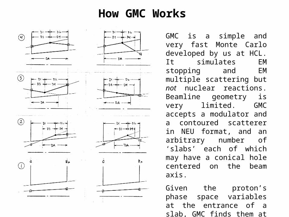
GMC is a simple and very fast Monte Carlo developed by us at HCL. It simulates EM stopping and EM multiple scattering but not nuclear reactions. Beamline geometry is very limited. GMC accepts a modulator and a contoured scatterer in NEU format, and an arbitrary number of ‘slabs’ each of which may have a conical hole centered on the beam axis.

Given the proton’s phase space variables at the entrance of a slab, GMC finds them at the exit. Four possible topologies are: 1) in the hole projected to stay in, 2) in projected to leave, 3) outside projected to enter the hole and 4) outside projected to stay outside.

How GMC Works

The distribution in angle (r′ = dr/dz = (x x′ + y y′)/r ) of inners is broadly peaked about the original proton direction. The dip marks the transition between Courant’s categories 2 and 3 (whether the proton emerges from the bore or the back face). Outers, by contrast, all head towards the axis with a mean angle ≈ 100 mrad = 6° , in excellent agreement with the early prediction of Burge and Smith (1962) for copper.

Angular Fluence Distributions

The energy spectrum of inners is peaked towards high energy (‘full’ energy, 201 MeV, is just off scale to the right). In other words, many protons just nip the far corner. By contrast, the outers are broadly spread between zero and maximum. That means many of them will have large stopping power! Incidentally, if the collimator was not subdivided into enough slabs for the simulation, a spurious periodicity will appear in this spectrum.

Energy Distributions

Proton angles are difficult to measure, but the transverse dose distribution is easy. The Monte Carlo lets us separate inners and outers, which would be combined in a simple transverse dose scan.

The inners are unremarkable; the dose spreads as we recede from the collimator.By contrast, the outers start just inside the bore and spread into the treatment field as they converge towards the axis. Eventually they cross over producing tails in the dose distribution. An ‘anti-scatter’ aperture behind the first one would not block any of these protons. However, many have short ranges and only contribute to the proximal dose.

Radial Dose Distributions

You might ask, ‘What fraction of the protons are slit-scattered?’ For inners, that fraction approaches a constant (in a typical beam) as the aperture is made larger. For outers we may define an equivalent annulus around the bore, hitting which a proton will scatter back out. Therefore the fraction depends on the ratio of circumference to area viz. 1/r. In effect (cf. Courant) the slit is slightly larger than its physical size. The formula for the dashed line shows that the relevant ‘skin depth’ is about 1 mm for a brass aperture.

Fraction of Protons Affected

Outline








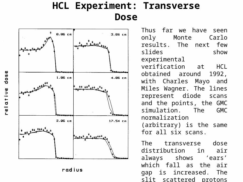
Thus far we have seen only Monte Carlo results. The next few slides show experimental verification at HCL obtained around 1992, with Charles Mayo and Miles Wagner. The lines represent diode scans and the points, the GMC simulation. The GMC normalization (arbitrary) is the same for all six scans.

The transverse dose distribution in air always shows ‘ears’ which fall as the air gap is increased. The slit scattered protons don’t vanish, of course. They approach the axis and spread out, becoming less obvious. Eventually they cross, causing the barely noticeable tails. The overall decrease in dose is due to 1/r2.

HCL Experiment: Transverse Dose

This figure from Van Luijk et al. (Phys. Med. Biol. 46 (2001) 653-670) shows the same general behavior of the transverse dose distribution. A pristine 150 MeV beam was double scattered into a 2 - 20 mm wide by 100 mm long (i.e. ‘1D’) slit designed for radiobiology on the rat spinal chord. The dose was measured with a CCD/scintillator system and simulated with GEANT 3.21 .

a) Dose ‘ears’ from outers emerging upstream from the slit bunch up in the center as the slit becomes smaller. b) At a larger gap the ears have moved in producing a rounded effect. In the case of the narrow slit they have crossed over producing the broad pedestal. c) At a still larger gap everything looks normal but, of course, the degraded protons are still there as shown by the very broad pedestal under the 2 mm plot.

KVI Experiment

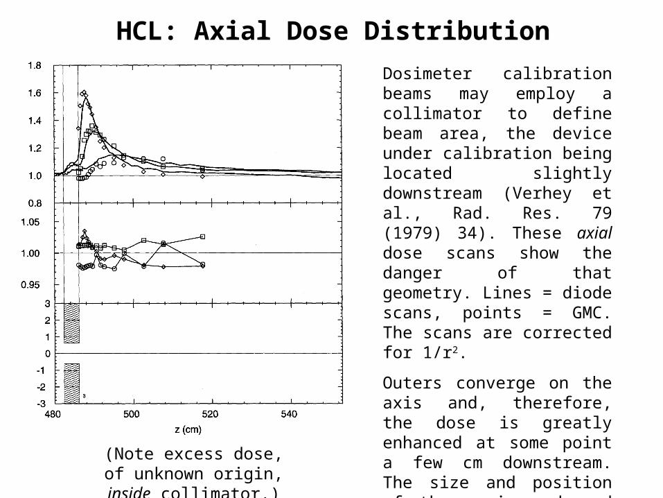
Dosimeter calibration beams may employ a collimator to define beam area, the device under calibration being located slightly downstream (Verhey et al., Rad. Res. 79 (1979) 34). These axial dose scans show the danger of that geometry. Lines = diode scans, points = GMC. The scans are corrected for 1/r2.

Outers converge on the axis and, therefore, the dose is greatly enhanced at some point a few cm downstream. The size and position of the maximum depend on the collimator radius.

Grusell et al. (Phys. Med. Biol. 40 (1995) 1831) calibrated a dosimeter in an uncollimated beam to avoid this problem.

(Note excess dose, of unknown origin, inside

collimator.)

HCL: Axial Dose Distribution

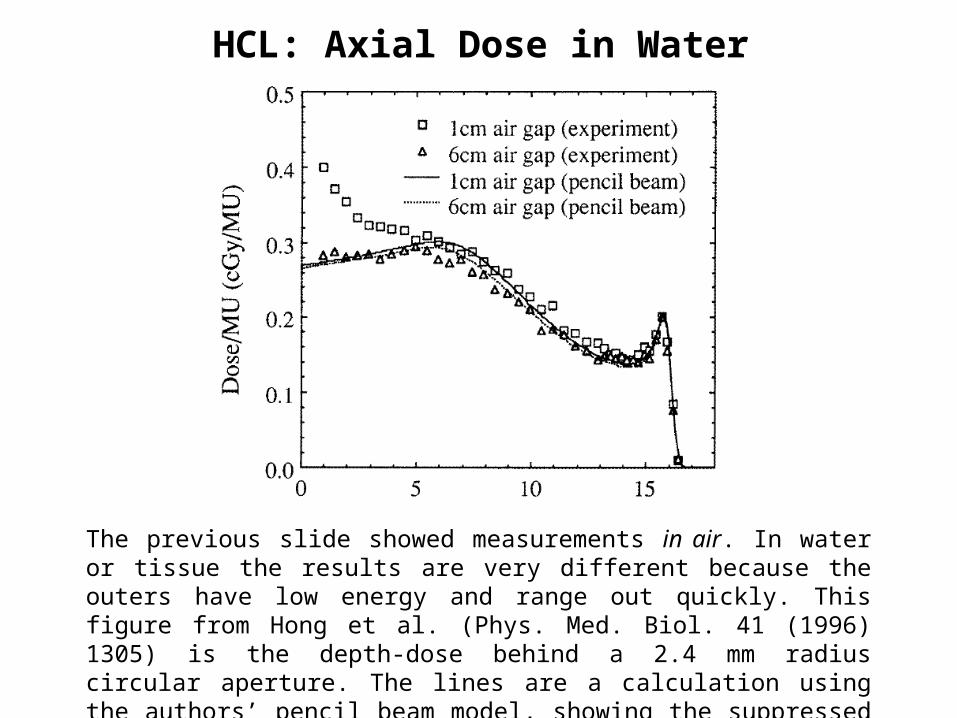
The previous slide showed measurements in air. In water or tissue the results are very different because the outers have low energy and range out quickly. This figure from Hong et al. (Phys. Med. Biol. 41 (1996) 1305) is the depth-dose behind a 2.4 mm radius circular aperture. The lines are a calculation using the authors’ pencil beam model, showing the suppressed Bragg peak. A large dose enhancement is seen at 1 cm air gap from outers. Slit scattering is not included in the theoretical model.

HCL: Axial Dose in Water

Finally, we ask whether GMC predicts the energy distribution correctly. One can measure this directly with a NaI scintillation spectrometer, but this is a difficult technique requiring the beam current to be lowered drastically. We eventually used a Multi-Layer Faraday Cup (MLFC) to measure the range distribution of outers in copper.

The full squares represent a very small uncollimated beam. The entrance region shows low energy proton secondaries from nuclear reactions, which stop early. The hollow squares are the range distribution of all protons emerging from a ½″ brass collimator. The line is GMC’s prediction of outers plus the measured contribution of nuclear events, which GMC does not know about.

HCL: Range Distribution with MLFC

Outline








Slit scattering is closely related to dose perturbation by an inhomogeneity. This figure from Goitein et al. (Med. Phys. 5 (1978) 265) shows the dose in air behind a thin Lucite sheet illuminated by 127 MeV protons. The line represents Goitein’s theoretical prediction (Med. Phys. 5 (1978) 258).

The dose enhancement just outside the geometrical shadow of the edge has exactly the same origin as our ‘outers’: protons that scatter out the edge. The dose defect just inside the shadow arises because those same protons were headed for that region but scattered out. The overall effect is bipolar with zero net area. With a slit, the ‘minus’ region has zero dose because the protons stop, so no defect is seen.

Dose Perturbation by an Inhomogeneity

Outline








Two very similar papers investigate the effect of finite slit thickness on transverse penumbra. Both consider the effect on a superposition of pencil beams grazing the slit, and both view the slit as two separated ideal slits. In other words, they do not treat slit scattering. This figure from Kanematsu et al. (Phys. Med. Biol. 51 (2006) 4807) shows how one edge or the other governs, depending on the proton angle. The right-hand panel is a phase space picture of the same thing.

Tunnel Effect(one part of the problem)

This figure is from Slopsema and Kooy (Phys. Med. Biol. 51 (2006) 5441). It is obvious that the 3D effect depends on the mix of proton angles. It is usually significant only if the slit edge in question is near the axis; otherwise, the downstream edge rules. Both papers develop analytical formulas to improve pencil beam dose algorithms.

In our view this partial treatment (3D effect only) is of limited value because slit scattering effects are of exactly the same order of magnitude.

Tunnel Effect(similar treatment, same journal, same

issue !)

Tunnel Effect (Experimental)

This analysis of Kooy’s data (BG, unpublished) shows the 80/20 penumbra at 20 cm air gap, as a function of the nozzle range setting, for no mod and full mod. As expected, the penumbra on axis exceeds that off axis by a small but perfectly reproducible amount.

Tunnel Effect (Experimental)

At 70 cm air gap the 80/20 penumbra is much larger. The absolute effect on/off axis is the same (as predicted by both papers) but is now overshadowed by the difference between no mod and full mod.

Outline








Taper

When the field is large the mean proton angle at the edge of the collimator is large and it is tempting to consider a tapered aperture. That is not trivial to fabricate for an irregular hole, because the optimum taper depends on how far the edge is from the beam axis.

Early measurements at the Burr Center (Miles Wagner, unpublished) show that the transverse penumbra in air is indeed smaller with a tapered edge. However, he did not study the energy distribution or the effect in a realistic treatment volume. Decreasing ‘inners’ with taper will increase ‘outers’ and the related dose to the proximal field, so there is a tradeoff.

To date, as far as we know, tapered apertures have not been used in proton radiotherapy.

Slit Material

Using GMC we did a quick study of different slit materials. The mean convergence angle of outers increases with Z: 2.1, 6.2, 8.3° for beryllium, brass, lead. The rms width of the angular distribution is a constant 75% of the mean angle.

The graph shows the percentage of inners and outers relative to pristines for a single scattered 158.6 MeV beam and a 1 cm radius collimator. Beryllium has fewer outers than brass, lead more, but the total fraction of slit scattered protons is least for brass.

There seems to be no general advantage in changing the material. Outers, which affect the treatment dose, may be worse for Cerrobend™ than for brass. Note: a recent paper suggests using plastic to reduce unwanted neutron dose to patient. The patient aperture becomes very thick.

Summary

Protons that interact with a collimator, lose energy and scatter, but do not stop, fall into two classes. ‘Inners’, which enter inside the physical bore, proceed more or less in their original direction with some energy loss and scatter. ‘Outers’ converge from the bore towards the axis with a typical angle of 6° (brass). In air, that can cause a large enhancement in the axial depth-dose. Later, the outers cross the axis causing a large divergent beam halo.

In water, the low energy and large dE/dx of outers causes a dose enhancement near the skin. The effect at depth is usually negligible.

Slit scattering can be described using only EM stopping and scattering. Nuclear reactions play a negligible role.

Collimators are the prime source of unwanted neutron dose to the patient. Unwanted protons should be stopped as soon as possible to take advantage of 1/r2 and to minimize collimator material. In a double scattering system this implies a collimator surrounding the second scatterer.

Despite some studies of the 3D effect by itself, a complete analytic description of protons interacting with a real aperture, in a form convenient to pencil beam algorithms, has yet to be found.

Documents

Slit Scattering Slits (or collimators, apertures) are used in proton beam lines to block unwanted protons. Usually, the further upstream we do this, the