Embed Size (px)
Citation preview

Slide 2- 1

Chapter 2
Polynomial, Power, and Rational Functions

2.1
Linear and Quadratic Functions and Modeling

Slide 2- 4
Quick Review
2
1. Write an equation in slope-intercept form for a line with slope 2 and
-intercept 10.
2. Write an equation for the line containing the points ( 2,3) and (3,
2 10
14 3
5
4).
3. Expand ( 6) .
m
y
x
y x
y x
2
22
22
12 36
4 12
4. Expand (2 3) .
5. Factor 2 8 8.
9
2 2
x x
x xx
x xx

Slide 2- 5
What you’ll learn about
Polynomial Functions Linear Functions and Their Graphs Average Rate of Change Linear Correlation and Modeling Quadratic Functions and Their Graphs Applications of Quadratic Functions
… and whyMany business and economic problems are modeled by linear functions. Quadratic and higher degree polynomial functions are used to model some manufacturing applications.

Slide 2- 6
Polynomial Function
0 1 2 1
1 2
1 2 1 0
Let be a nonnegative integer and let , , ,..., , be real numbers with
0. The function given by ( ) ...
is a .
The
n n
n n
n n n
n a a a a a
a f x a x a x a x a x a
polynomial function of degree
leading coeffi
n
is .n
acient

Slide 2- 7
Polynomial Functions of No and Low Degree
Name Form DegreeZero Function f(x) = 0 Undefined
Constant Function f(x) = a (a ≠ 0) 0
Linear Function f(x)=ax + b (a ≠ 0) 1
Quadratic Function f(x)=ax2 + bx + c (a ≠ 0) 2

Slide 2- 8
Example Finding an Equation of a Linear Function
Write an equation for the linear function such that (-1) 2 and (2) 3.f f f
1 1
The line contains the points (-1,2) and (2,3). Find the slope:
3 2 1
2 1 3Use the point-slope formula and the point (2,3):
( )
13 2
31 2
33 3
1 7
3 31 7
( )3 3
m
y y m x x
y x
y x
y x
f x x

Slide 2- 9
Average Rate of Change
The average rate of change of a function ( ) between and ,
( ) ( ), is .
y f x x a x b
f b f aa b
b a

Slide 2- 10
Constant Rate of Change Theorem
A function defined on all real numbers is a linear
function if and only if it has a constant nonzero
average rate of change between any two points
on its graph.
Slide 2- 11
Characterizing the Nature of a Linear Function
Point of View Characterization
Verbal polynomial of degree 1
Algebraic f(x) = mx + b (m ≠ 0)
Graphical slant line with slope m and y-intercept b
Analytical function with constant nonzero rate of change m:
f is increasing if m > 0, decreasing if m < 0; initial
value of the function = f(0) = b

Slide 2- 12
Properties of the Correlation Coefficient, r
1. -1 ≤ r ≤ 12. When r > 0, there is a positive linear
correlation.3. When r < 0, there is a negative linear
correlation.4. When |r| ≈ 1, there is a strong linear
correlation.5. When |r| ≈ 0, there is weak or no linear
correlation.

Slide 2- 13
Linear Correlation

Slide 2- 14
Regression Analysis
1. Enter and plot the data (scatter plot).
2. Find the regression model that fits the problem situation.
3. Superimpose the graph of the regression model on the scatter plot, and observe the fit.
4. Use the regression model to make the predictions called for in the problem.

Slide 2- 15
Example Transforming the Squaring Function
2
2
Describe how to transform the graph of ( ) into the graph of
( ) 2 2 3.
f x x
f x x

Slide 2- 16
Example Transforming the Squaring Function
2
2
Describe how to transform the graph of ( ) into the graph of
( ) 2 2 3.
f x x
f x x
2
2
The graph of ( ) 2 2 3 is obtained by vertically stretching the
graph of ( ) by a factor of 2 and translating the resulting graph
2 units right and 3 units up.
f x x
f x x

Slide 2- 17
The Graph of f(x)=ax2

Slide 2- 18
Vertex Form of a Quadratic Equation
Any quadratic function f(x) = ax2 + bx + c, a ≠ 0, can be written in the vertex form
f(x) = a(x – h)2 + k
The graph of f is a parabola with vertex (h,k) and axis x = h, where h = -b/(2a) and
k = c – ah2. If a > 0, the parabola opens upward, and if a < 0, it opens downward.

Slide 2- 19
Find the vertex and the line of symmetryof the graph y = (x – 1)2 + 2
DomainRange
(- , )
[2, )
Vertex (1,2) x = 1

Slide 2- 20
Find the vertex and the line of symmetryof the graph y = -(x + 2)2 - 3
DomainRange
(- , )
(-,-3]
Vertex (-2,-3) x = -2

Slide 2- 21
Let f(x) = x2 + 2x + 4. (a) Write f in standard form. (b) Determine the vertex of f. (c) Is the vertex a maximum or a minimum? Explain
f(x) = x2 + 2x + 4
f(x) = (x + 1)2 + 3
Vertex (-1,3) opens up(-1,3) is a minimum
+ 1 - 1

Slide 2- 22
Let f(x) = 2x2 + 6x - 8. (a) Write f in standard form. (b) Determine the vertex of f. (c) Is the vertex a maximum or a minimum? Explain
f(x) = 2(x + 3/2)2 - 25/2
Vertex (-3/2,-25/2) opens up(-3/2,25/2) is a minimum
+ 9/4 - 9/2f(x) = 2(x2 + 3x ) - 8

Slide 2- 23
If we perform completing the square process on f(x) = ax2 + bx + c and write it in standard form, we get
cbxaxxf 2)(
cxa
bxaxf )()( 2
a
bc
a
bx
a
bxaxf
4)
4()(
2
2
22

Slide 2- 24
a
bc
a
bx
a
bxaxf
4)
4()(
2
2
22
a
bc
a
bxaxf
42)(
22
So the vertex is
a
bc
a
b
4,
2
2

Slide 2- 25
ab
fa
b2
,2
To get the coordinates of the vertex of any quadratic function, simply use the vertex formula.
• If a > 0, the parabola open up and the vertex is a minimum.
• If a < 0, the parabola opens down and the parabola is a maximum.

Slide 2- 26
Example Finding the Vertex and Axis of a Quadratic Function
2
Use the vertex form of a quadratic function to find the vertex and axis
of the graph of ( ) 2 8 11. Rewrite the equation in vertex form. f x x x
2
2
The standard polynomial form of is ( ) 2 8 11.
So 2, 8, and 11, and the coordinates of the vertex are
82 and ( ) (2) 2(2) 8(2) 11 3.
2 4The equation of the axis is 2, the vertex
f f x x x
a b c
bh k f h f
ax
2
is (2,3), and the
vertex form of is ( ) 2( 2) 3.f f x x

Slide 2- 27
Characterizing the Nature of a Quadratic Function
Point of View Characterization
2
2
Verbal polynomial of degree 2
Algebraic ( ) or
( ) ( - ) ( 0)
Graphical parabola with vertex ( , ) and
axis ; opens upward if >
f x ax bx c
f x a x h k a
h k
x h a
0,
opens downward if < 0;
initial value = -intercept = (0)
-intercept
a
y f c
x
2 4
s2
b b ac
a

Slide 2- 28
Vertical Free-Fall Motion
2
0 0 0
2 2
The and vertical of an object in free fall are given by
1( ) and ( ) ,
2where is time (in seconds), 32 ft/sec 9.8 m/sec is the
,
s v
s t gt v t s v t gt v
t g
height velocity
acceleration
due to gravity0 0
is the of the object, and is its
.
v initial vertical velocity s
initial height

2.2
Power Functions and Modeling

Slide 2- 30
Quick Review
5 / 3
-3
1.
3
5
5
3
3
Write the following expressions using only positive integer powers.
1.
2.
3.
Write the following expressions in the form using a single rational
number for the powe
1
r
a
x
r
m
k x
x
r
m
3
2
1
3
33
of .
4. 16
5.
4
1
27 3
x
x
x
a
x

Slide 2- 31
What you’ll learn about
Power Functions and Variation Monomial Functions and Their Graphs Graphs of Power Functions Modeling with Power Functions
… and whyPower functions specify the proportional relationships of geometry, chemistry, and physics.

Slide 2- 32
Power Function
Any function that can be written in the formf(x) = k·xa, where k and a are nonzero constants,is a power function. The constant a is the power, and the k is the constant of variation,
or constant of proportion. We say f(x) varies as the ath power of x, or f(x) is proportional to the ath power of x.

Slide 2- 33
Example Analyzing Power Functions
4State the power and constant of variation for the function ( ) ,
and graph it.
f x x
1/ 4 1/ 44( ) 1 so the power is 1/4 and
the constant of variation is 1.
f x x x x

Slide 2- 34
Monomial Function
Any function that can be written as
f(x) = k or f(x) = k·xn, where k is a constant and n is a positive integer, is a monomial function.

Slide 2- 35
Example Graphing Monomial Functions
3Describe how to obtain the graph of the function ( ) 3 from the graph
of ( ) with the same power .n
f x x
g x x n
3
3
We obtain the graph of ( ) 3 by vertically stretching the graph of
( ) by a factor of 3. Both are odd functions.
f x x
g x x

Slide 2- 36
Graphs of Power Functions
For any power function f(x) = k·xa, one of the
following three things happens when x < 0. f is undefined for x < 0. f is an even function. f is an odd function.

Slide 2- 37
Graphs of Power Functions

2.3
Polynomial Functions of Higher Degree with Modeling

Slide 2- 39
Quick Review
2
3 2
2
3
Factor the polynomial into linear factors.
1. 3 11 4
2. 4 10 24
Solve the equation mentally.
3. ( 2) 0
4. 2( 2) ( 1) 0
3 1 4
2 2 3 4
0,
5. ( 3)(
2
2, 1
5) 0
x x
x x x
x x
x x
x x x
x x
x x x
x x
x x
0, 3, 5x x x

Slide 2- 40
What you’ll learn about
Graphs of Polynomial Functions End Behavior of Polynomial Functions Zeros of Polynomial Functions Intermediate Value Theorem Modeling
… and whyThese topics are important in modeling and can be used to provide approximations to more complicated functions, as you will see if you study calculus.

Slide 2- 41
The Vocabulary of Polynomials
1
1 0 Each monomial in the sum , ,..., is a of the polynomial.
A polynomial function written in this way, with terms in descending degree,
is written in .
The constan
n n
n na x a x a
term
standard form
1 0
0
ts , ,..., are the of the polynomial.
The term is the , and is the constant term.n n
n
n
a a a
a x a
coefficients
leading term

Slide 2- 42
Example Graphing Transformations of Monomial Functions
4
Describe how to transform the graph of an appropriate monomial function
( ) into the graph of ( ) ( 2) 5. Sketch ( ) and
compute the -intercept.
n
nf x a x h x x h x
y
4
4
4
You can obtain the graph of ( ) ( 2) 5 by shifting the graph of
( ) two units to the left and five units up. The -intercept of ( )
is (0) 2 5 11.
h x x
f x x y h x
h

Slide 2- 43
Cubic Functions

Slide 2- 44
Quartic Function

Slide 2- 45
Local Extrema and Zeros of Polynomial Functions
A polynomial function of degree n has at most
n – 1 local extrema and at most n zeros.

Slide 2- 46
Leading Term Test for Polynomial End Behavior
1 0For any polynomial function ( ) ... , the limits lim ( ) and
lim ( ) are determined by the degree of the polynomial and its leading
coefficient :
n
n x
x
n
f x a x a x a f x
f x n
a

Slide 2- 47
Example Applying Polynomial Theory
4 3Describe the end behavior of ( ) 2 3 1 using limits.g x x x x
lim ( )x
g x
Slide 2- 48
Example Finding the Zeros of a Polynomial Function
3 2Find the zeros of ( ) 2 4 6 .f x x x x
3 2
Solve ( ) 0
2 4 6 0
2 1 3 0
0, 1, 3
f x
x x x
x x x
x x x

Slide 2- 49
Multiplicity of a Zero of a Polynomial Function
1
If is a polynomial function and is a factor of
but is not, then is a zero of of .
m
m
f x c f
x c c f
multiplicity m

Slide 2- 50
Example Sketching the Graph of a Factored Polynomial
3 2Sketch the graph of ( ) ( 2) ( 1) .f x x x
The zeros are 2 and 1. The graph crosses the -axis at 2 because
the multiplicity 3 is odd. The graph does not cross the -axis at 1 because
the multiplicity 2 is even.
x x x x
x x

Slide 2- 51
Intermediate Value Theorem
If a and b are real numbers with a < b and if f is
continuous on the interval [a,b], then f takes on
every value between f(a) and f(b). In other
words, if y0 is between f(a) and f(b), then y0=f(c)
for some number c in [a,b].

2.4
Real Zeros of Polynomial Functions

Slide 2- 53
Quick Review
3 2
5 3 2
2
3
3 2
2
3
Rewrite the expression as a polynomial in standard form.
2 31.
2 82.
2Factor the polynomial into linear factors.
3. 16
4. 4
2 3 1
14
2
4 4
4 2 1 2
x x
x x
x
x x x
xx x x
x
x x
x x
x x
x x xx
25. 6 24 2 2 6 x xx

Slide 2- 54
What you’ll learn about
Long Division and the Division Algorithm Remainder and Factor Theorems Synthetic Division Rational Zeros Theorem Upper and Lower Bounds
… and whyThese topics help identify and locate the real zeros of polynomial functions.

Slide 2- 55
QuotientDividendDivisor
Remainder
Check:
Quotient * Divisor + Remainder = Dividend
Division

Slide 2- 56
Division Algorithm for Polynomials
Let ( ) and ( ) be polynomials with the degree of greater than or equal to the
degree of , and ( ) 0. Then there are unique polynomials ( ) and ( ),
called the and , such th
f x d x f
d d x q x r xquotient remainder at ( ) ( ) ( ) ( )
where either ( ) 0 or the degree of is less than the degree of .
The function ( ) in the division algorithm is the , and ( ) is the .
If ( ) 0, we say ( )
f x d x q x r x
r x r d
f x d x
r x d x
dividend divisor
di into ( ).f xvides evenly

Slide 2- 57
Dividing Polynomials
Long division of polynomials is similar to long division of whole numbers.
dividend = (quotient • divisor) + remainder
The result is written in the form:
quotient +divisor
remainder divisor dividend
When you divide two polynomials you can check the answer using the following:

Slide 2- 58
+ 2 2 3 1 2 xxx
Example: Divide x2 + 3x – 2 by x + 1 and check the answer.
x
x2 + x2x – 22x + 2
– 4
remainder
Check:
xx
xxx
22 1.
xxxx 2)1(2.
xxxxx 2)()3( 22 3.
22
2 x
xxx4.
22)1(2 xx5.
4)22()22( xx6.
correct(x + 2)
quotient
(x + 1)
divisor
+ (– 4)
remainder
= x2 + 3x – 2
dividend
Answer: x + 2 +1x
– 4

Slide 2- 59
Example: Divide 4x + 2x3 – 1 by 2x – 2 and check the answer.
1 4 0 2 2 2 23 xxxx Write the terms of the dividend in
descending order.
23
2
2x
x
x1.
x2
232 22)22( xxxx 2.
2x3 – 2x2
2233 2)22(2 xxxx 3.
2x2 + 4x
xx
x
2
2 2
4.
+ x
xxxx 22)22( 2 5.
2x2 – 2x
xxxxx 6)22()42( 22 6.
6x – 1
32
6
x
x7.
+ 3
66)22(3 xx8.
6x – 6
remainder5)66()16( xx9.
5
Check: (x2 + x + 3)(2x – 2) + 5
= 4x + 2x3 – 1
Answer: x2 + x + 322
x5
Since there is no x2 term in the
dividend, add 0x2 as a placeholder.
Slide 2- 60
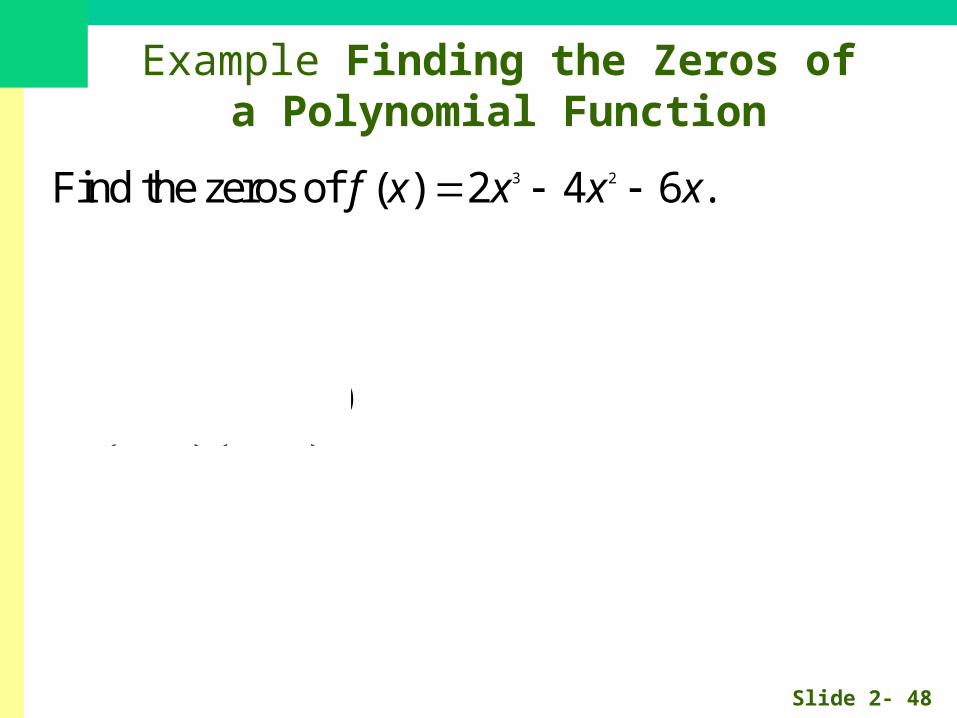
6 5 2 2 xxxx
x2 – 2x
– 3x + 6
– 3
– 3x + 60
Answer: x – 3 with no remainder.
Check: (x – 2)(x – 3) = x2 – 5x + 6
Example: Divide x2 – 5x + 6 by x – 2.

Slide 2- 61
Example: Divide x3 + 3x2 – 2x + 2 by x + 3 and check the answer.
2 2 3 3 23 xxxx
x2
x3 + 3x2
0x2 – 2x
– 2
– 2x – 6
8
Check: (x + 3)(x2 – 2) + 8
= x3 + 3x2 – 2x + 2
Answer: x2 – 2 +3x
8
+ 2
Note: the first subtraction
eliminated two terms from
the dividend.
Therefore, the quotient
skips a term.
+ 0x

Slide 2- 62
16
Synthetic division is a shorter method of dividing polynomials.
This method can be used only when the divisor is of the form
x – a. It uses the coefficients of each term in the dividend.
Example: Divide 3x2 + 2x – 1 by x – 2 using synthetic division.
3 2 – 12
Since the divisor is x – 2, a = 2.
3
1. Bring down 3
2. (2 • 3) = 6
6
8 15
3. (2 + 6) = 8
4. (2 • 8) = 16
5. (–1 + 16) = 15coefficients of quotient remainder
value of a coefficients of the dividend
3x + 8Answer: 2
x15

Slide 2- 63
Example: Divide x3 – 3x + 4 by x + 3 using synthetic division.
Notice that the degree of the first term of the quotient is one less
than the degree of the first term of the dividend.
remainder
)3()43( 3 xxx
a
coefficients of quotient
– 3
Since, x – a = x + 3, a = – 3.
1 0 – 3 4
1
– 3
– 3
9 – 18
6 – 14
coefficients of dividend
= x2 – 3x + 6 3
x– 14
Insert zero coefficient
as placeholder for the
missing x2 term.

Slide 2- 64
Remainder Theorem: The remainder of the division of a
polynomial f (x) by x – a is f (a).
Example: Using the remainder theorem, evaluate
f(x) = x 4 – 4x – 1 when x = 3.
9
1 0 0 – 4 – 13
1
3
3 9
6927
23 68
The remainder is 68 at x = 3, so f (3) = 68.
You can check this using substitution: f(3) = (3)4 – 4(3) – 1 = 68.
value of x

Slide 2- 65
Example: Using synthetic division and the remainder theorem,
evaluate f (x) = x2 – x at x = – 2.
6
1 – 1 0– 2
1
– 2
– 3 6
Then f (– 2) = 6 and (– 2, 6) is a point on the graph of f(x) = x2 – x.
f(x) = x2 – x
x
y
2
4
(– 2, 6)
remainder

Slide 2- 66
Example Using Polynomial Long Division
4 3
2
Use long division to find the quotient and remainder when 2 3
is divided by 1.
x x
x x

Slide 2- 67
Example Using Polynomial Long Division
4 3
2
Use long division to find the quotient and remainder when 2 3
is divided by 1.
x x
x x
2
2 4 3 2
4 3 2
3 2
3 2
2
2
4 3 2 2
2
2 11 2 0 0 3
2 2 2
2 0 3
+ 3
1
2 2
2 22 3 1 2 1
1
x xx x x x x x
x x x
x x x
x x x
x x
x x
x
xx x x x x x
x x

Slide 2- 68
Remainder Theorem
If polynomial ( ) is divided by , then the remainder is ( ).f x x k r f k

Slide 2- 69
Example Using the Remainder Theorem
2Find the remainder when ( ) 2 12 is divided by 3.f x x x x
2
( 3) 2 3 3 12 =33r f

Slide 2- 70
Factor Theorem
A polynomial function ( ) has a factor if and only if ( ) 0.f x x k f k

Slide 2- 71
Example Using Synthetic Division
3 2Divide 3 2 5 by 1 using synthetic division.x x x x
1 3 2 1 5
3
1 3 2 1 5
3 1 2
3 1 2 3
3 2
23 2 5 33 2
1 1
x x xx x
x x

Slide 2- 72
Rational Zeros Theorem
1
1 0
0
Suppose is a polynomial function of degree 1 of the form
( ) ... , with every coefficient an integer
and 0. If / is a rational zero of , where and have
no common integ
n n
n n
f n
f x a x a x a
a x p q f p q
0
er factors other than 1, then
is an integer factor of the constant coefficient , and
is an integer factor of the leading coefficient .n
p a
q a

Slide 2- 73
Upper and Lower Bound Tests for Real Zeros
Let be a polynomial function of degree 1 with a positive leading
coefficient. Suppose ( ) is divided by using synthetic division.
If 0 and every number in the last line is nonnegative (po
f n
f x x k
k
sitive or zero),
then is an for the real zeros of .
If 0 and the numbers in the last line are alternately nonnegative and
nonpositive, then is a for the real zeros of .
k upper bound f
k
k lower bound f

Slide 2- 74
Show 2x - 3 is a factor of 6x2 + x – 15
(x = 3/2) 3/2 6 1 -15
6
9
10
15
0
Note: Since theremainder is 0, 2x - 3 is a factor
of 6x2 + x – 15

Slide 2- 75
Factor x4 – 3x3 – 5x2 + 3x + 4 )4(),2(),1( xxxare possible factors
P(1) = 0
1 1 -3 -5 3 4
1
1
-2
-2
-7
-7
-4
-4
0
x3 – 2x2 – 7x - 4
so x4 – 3x3 – 5x2 + 3x + 4 = (x3 – 2x2 – 7x – 4)(x – 1)

Slide 2- 76
Factor x3 – 2x2 – 7x - 4 )4(),2(),1( xxxare possible factors
P(-1) = 0
-1 1 -2 -7 -4
1
-1
-3
3
-4
4
0
x2 – 3x – 4
so x4 – 3x3 – 5x2 + 3x + 4 = (x2 – 3x – 4)(x – 1)(x + 1)

Slide 2- 77
Factor x3 – 2x2 – 7x - 4 )4(),2(),1( xxxare possible factors
P(-1) = 0
-1 1 -2 -7 -4
1
-1
-3
3
-4
4
0
x2 – 3x – 4
so x4 – 3x3 – 5x2 + 3x + 4 = (x2 – 3x – 4)(x – 1)(x + 1)

Slide 2- 78
•x4 – 3x3 – 5x2 + 3x + 4 = (x2 – 3x – 4)(x – 1)(x + 1)• or (x – 4)(x + 1)(x – 1)(x + 1)

Slide 2- 79
Factor x4 – 8x3 +17x2 + 2x - 24
)24)(12(
)8(),6(),4(
)3(),2(),1(
xx
xxx
xxx
are possible factorsP(4) = 0
4 1 -8 17 2 -24
1
4
-4
-16
1
4
6
24
0
x3 – 4x2 + x + 6
so x4 – 8x3 + 17x2 + 2x - 24 = (x3 – 4x2 + x + 6)(x – 4)

Slide 2- 80
Factor x3 – 4x2 + x + 6
P(2) = 0
2 1 -4 1 6
1
2
-2
-4
-3
-6
0
x2 – 2x – 3
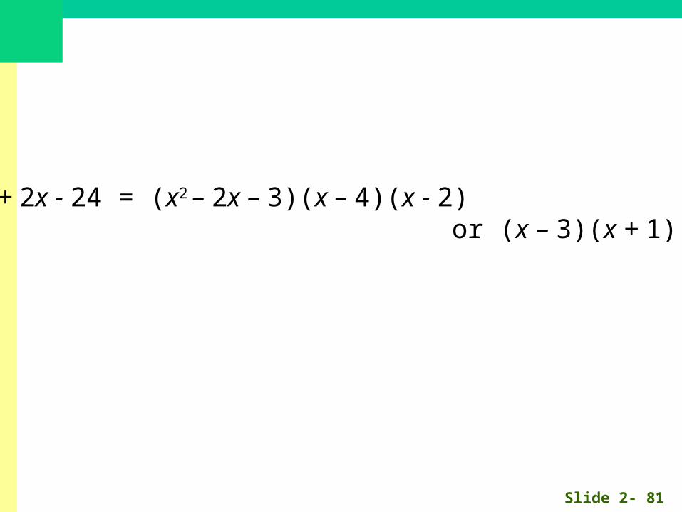
so x4 – 8x3 +17x2 + 2x - 24 = (x2 – 2x – 3)(x – 4)(x - 2)
)24)(12(
)8(),6(),4(
)3(),2(),1(
xx
xxx
xxx
are possible factors
Slide 2- 81
•x4 – 8x3 +17x2 + 2x - 24 = (x2 – 2x – 3)(x – 4)(x - 2)• or (x – 3)(x + 1)(x – 4)(x - 2)

Slide 2- 82
•Show x3 – 3x2 + 5 = 0 has no rational roots
1, 5 only possible roots
P(1) = 13 – 3(1)2 + 5 = 3
P(-1) = (-1)3 – 3(-1)2 + 5 = 1
P(5) = (5)3 – 3(5)2 + 5 = 55
P(-5) = (-5)3 – 3(-5)2 + 5 = -195
Since none of the possible roots give zero in the remaindertheorem, there are norational roots.
Slide 2- 83
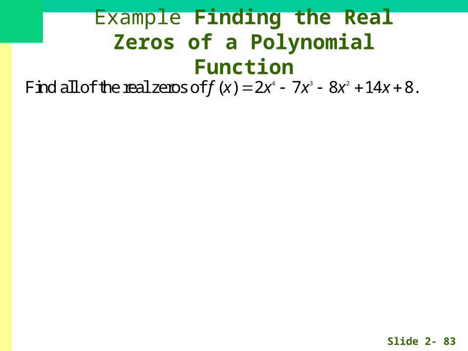
Example Finding the Real Zeros of a Polynomial Function
4 3 2Find all of the real zeros of ( ) 2 7 8 14 8.f x x x x x

Slide 2- 84
Example Finding the Real Zeros of a Polynomial Function
4 3 2Find all of the real zeros of ( ) 2 7 8 14 8.f x x x x x
:
Factors of 8 1, 2, 4, 8 1: 1, 2, 4, 8,
Factors of 2 1, 2 2
Compare the -intercepts of the graph and the list of possibilities,
and decide that 4 and -1/2 are potential rational
Potential Rational Zeros
x
zeros.

Slide 2- 85
Example Finding the Real Zeros of a Polynomial Function
4 3 2 3 2
4 2 7 8 14 8
8 4 16 8
2 1 4 2 0
This tells us that 2 7 8 14 8 ( 4)(2 4 2).
1/ 2
x x x x x x x x
4 3 2 2
2 1 4 2
1 0 2
2 0 4 0
1This tells us that 2 7 8 14 8 2( 4) 2 .
2
1The real zeros are 4,
x x x x x x x
, 2.2
4 3 2Find all of the real zeros of ( ) 2 7 8 14 8.f x x x x x

2.5
Complex Zeros and the Fundamental Theorem of Algebra

Slide 2- 87
Quick Review
2
1
Perform the indicated operation, and write the result in the form .
1. 2 3 1 5
2. 3 2 3 4
Factor the quadratic equation.
3. 2 9 5
Solve the quadratic equatio
8
1 18
2 1 5
n.
a bi
i i
i i
i
i
x xx x
2
4 2
4. 6 10 0
List all potential rational zeros.
3
2, 1, 15. 4 3 2 / 2, 1/ 4
x x
x x
x i
x

Slide 2- 88
What you’ll learn about
Two Major Theorems Complex Conjugate Zeros Factoring with Real Number Coefficients
… and whyThese topics provide the complete story about the zeros and factors of polynomials with real number coefficients.

Slide 2- 89
Fundamental Theorem of Algebra
A polynomial function of degree n has n complex zeros (real and nonreal). Some of these zeros may be repeated.

Slide 2- 90
Linear Factorization Theorem
1 2
1 2
If ( ) is a polynomial function of degree 0, then ( ) has precisely
linear factors and ( ) ( )( )...( ) where is the
leading coefficient of ( ) and , ,..., are the complex zen
n
f x n f x
n f x a x z x z x z a
f x z z z
ros of ( ).
The are not necessarily distinct numbers; some may be repeated.i
f x
z

Slide 2- 91
Fundamental Polynomial Connections in the Complex Case
The following statements about a polynomial function f are equivalent if k is a complex number:
1. x = k is a solution (or root) of the equation f(x) = 0
2. k is a zero of the function f.
3. x – k is a factor of f(x).

Slide 2- 92
Example Exploring Fundamental Polynomial Connections
Write the polynomial function in standard form, identify the zeros of the function
and the -intercepts of its graph.
( ) ( 3 )( 3 )
x
f x x i x i
2The function ( ) ( 3 )( 3 ) 9 has two zeros:
3 and 3 . Because the zeros are not real, the
graph of has no -intercepts.
f x x i x i x
x i x i
f x

Slide 2- 93
Complex Conjugate Zeros
Suppose that ( ) is a polynomial function with real coefficients. If and are
real numbers with 0 and is a zero of ( ), then its complex conjugate
is also a zero of ( ).
f x a b
b a bi f x
a bi f x

Slide 2- 94
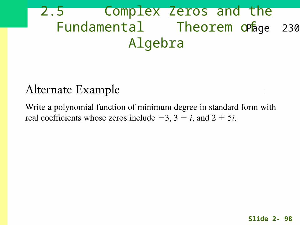
Example Finding a Polynomial from Given Zeros
Write a polynomial of minimum degree in standard form with real
coefficients whose zeros include 2, 3, and 1 .i
Because 2 and 3 are real zeros, 2 and 3 must be factors.
Because the coefficients are real and 1 is a zero, 1 must also
be a zero. Therefore, (1 ) and (1 ) must be factors.
( ) - 2 3 [
x x
i i
x i x i
f x x x x
2 2
4 3 2
(1 )][ (1 )]
( 6)( 2 2)
6 14 12
i x i
x x x x
x x x x

Slide 2- 95
Factors of a Polynomial with Real Coefficients
Every polynomial function with real coefficients can be written as a product of linear factors and irreducible quadratic factors, each with real coefficients.

Slide 2- 96
Find an equation of a polynomial with roots of 2i and 3.
(x – 2i)(x + 2i)(x – 3) = 0
(x2 – 2ix + 2ix – 4i2)(x – 3) = 0
(x2 + 4)(x – 3) = 0
x3 – 3x2 + 4x – 12 = 0

Slide 2- 97
Find an equation of a polynomial with roots of 1- i and -2.
(x – (1 - i))(x – (1 + i))(x + 2) = 0
(x2 – x - ix – x + 1 + i +ix -i - i2)(x + 2) = 0
(x2 – 2x + 2)(x + 2) = 0x3 + 2x2 –2x2 - 4x + 2x + 4= 0
(x – 1 + i)(x – 1 - i)(x + 2) = 0
x3 - 2x + 4 = 0
Slide 2- 98
2.5 Complex Zeros and the Fundamental Theorem of Algebra
Page 230

Slide 2- 99
2.5 Complex Zeros and the Fundamental Theorem of Algebra (cont’d)
Page 230

Slide 2- 100
Example Factoring a Polynomial
5 4 3 2Write ( ) 3 24 8 27 9as a product of linear and
irreducible quadratic factors, each with real coefficients.
f x x x x x x

Slide 2- 101
Example Factoring a Polynomial
5 4 3 2Write ( ) 3 24 8 27 9as a product of linear and
irreducible quadratic factors, each with real coefficients.
f x x x x x x
The Rational Zeros Theorem provides the candidates for the rational
zeros of . The graph of suggests which candidates to try first.
Using synthetic division, find that 1/ 3 is a zero. Thus,
( ) 3
f f
x
f x x
5 4 3 2
4 2
2 2
2
24 8 27 9
1 3 8 9
3
1 3 9 1
3
1 3 3 3 1
3
x x x x
x x x
x x x
x x x x

2.6
Graphs of Rational Functions

Slide 2- 103
Quick Review
2
2
2
3
Use factoring to find the real zeros of the function.
1. ( ) 2 7 6
2. ( ) 16
3 / 2, 2
4
no real z
3. ( ) 16
4. ( ) 27
eros
Find the quotient and r
3
emainder
f x x x
f x x
f x x
f x x
x x
x
x
when ( ) is divided by ( ).
5. ( ) 5 3, ( ) 5; 3
f x d x
f x x d x x
Slide 2- 104
What you’ll learn about
Rational Functions Transformations of the Reciprocal Function Limits and Asymptotes Analyzing Graphs of Rational Functions
… and whyRational functions are used in calculus and in scientific applications such as inverse proportions.

Slide 2- 105
Rational Functions
Let and be polynomial functions with ( ) 0. Then the function
( )given by ( ) is a .
( )
f g g x
f xr x
g x
rational function

Slide 2- 106
Example Finding the Domain of a Rational Function
Find the domain of and use limits to describe the behavior at
value(s) of not in its domain.
2( )
2
f
x
f xx
2 2
The domain of is all real numbers 2.
Use a graph of the function to find
lim ( ) and lim ( ) .x x
f x
f x f x
Slide 2- 107
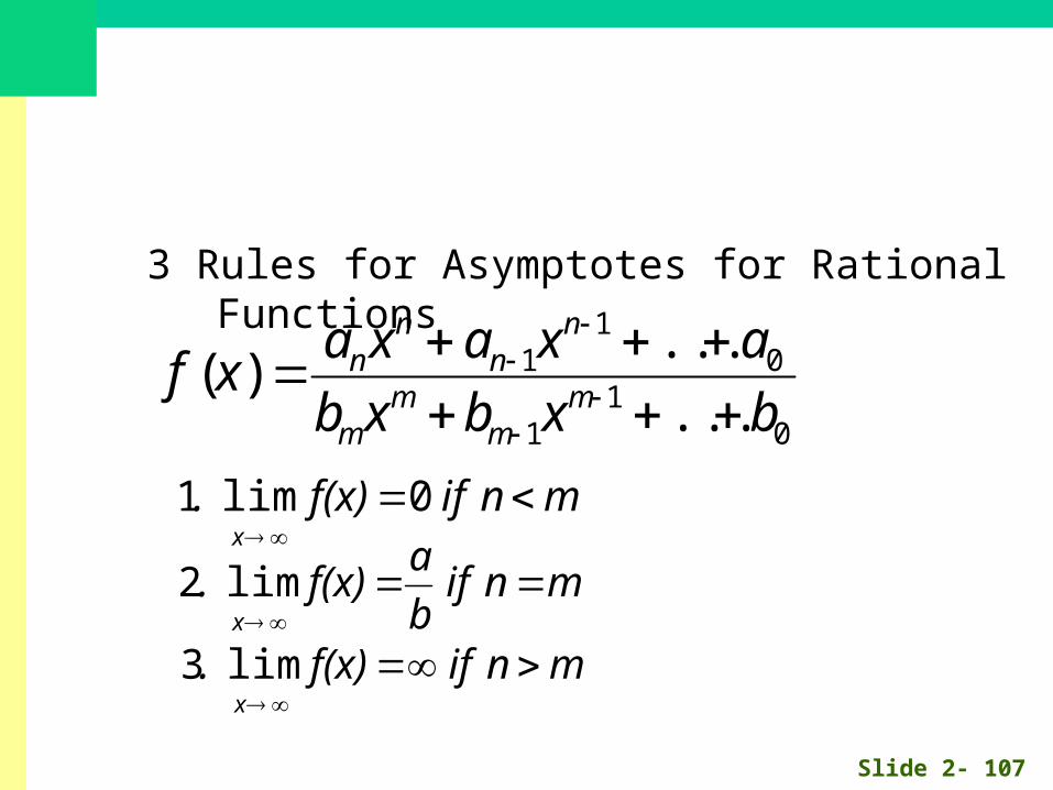
3 Rules for Asymptotes for Rational Functions
01
1
01
1
...
...)(
bxbxb
axaxaxf
mm
mm
nn
nn
mniff(x).x
0lim1
mnifb
af(x).
x
lim2
mniff(x).x
lim3

Slide 2- 108
Graph a Rational Function
The graph of ( ) / ( ) ( ...) /( ...) has the following
characteritics:
If , the end behavior asymptote is the horizontal asymptote 0.
If , the end behavior as
n m
n my f x g x a x b x
n m y
n m
1. End behavior asymptote :
ymptote is the horizontal asymptote / .
If , the end behavior asymptote is the quotient polynomial function
( ), where ( ) ( ) ( ) ( ). There is no horizontal asymptote.
n my a b
n m
y q x f x g x q x r x
Slide 2- 109
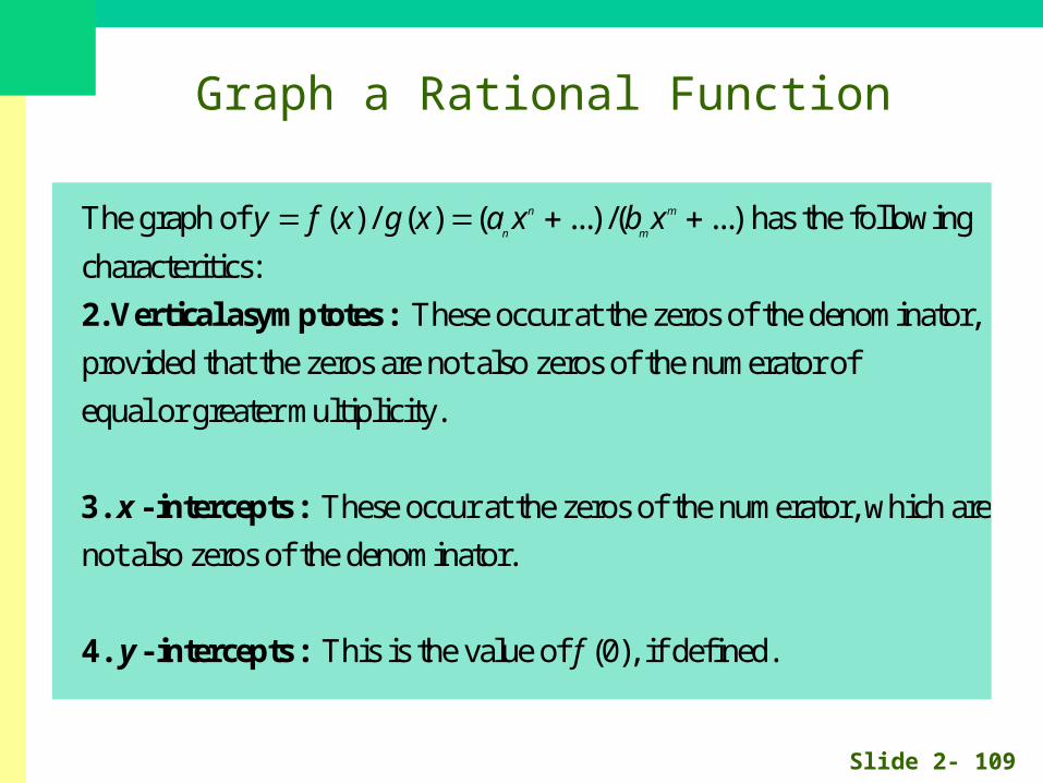
Graph a Rational Function
The graph of ( ) / ( ) ( ...) /( ...) has the following
characteritics:
These occur at the zeros of the denominator,
provided that the zeros are not also zeros of the nu
n m
n my f x g x a x b x
2. Vertical asymptotes :
merator of
equal or greater multiplicity.
These occur at the zeros of the numerator, which are
not also zeros of the denominator.
This is the value of (0), if defined.f
- intercepts :
- intercepts :
x
y
3.
4.

Slide 2- 110
Example Finding Asymptotes of Rational Functions
2( 3)( 3)Find the asymoptotes of the function ( ) .
( 1)( 5)
x xf x
x x
There are vertical asymptotes at the zeros of the denominator:
1 and 5.
The end behavior asymptote is at 2.
x x
y

Slide 2- 111
Example Graphing a Rational Function
1
Find the asymptotes and intercepts of ( ) and graph ( ).2 3
xf x f x
x x
The numerator is zero when 1 so the -intercept is 1. Because (0) 1/ 6,
the -intercept is 1/6. The denominator is zero when 2 and 3, so
there are vertical asymptotes at 2 and 3. The degree
x x f
y x x
x x
of the numerator
is less than the degree of the denominator so there is a horizontal asymptote
at 0.y
-3 1 2
----- ++++++ 0 ---- ++++++

Slide 2- 112
Sketch the graph of 1
3)(
x
xxf
f(0) = -3
Solve x – 3 = 0; x = 3
Solve x + 1 = 0; x = -1 and sketch the asymptote.
Horizontal asymptote, y = 1
-3 1
+++ --------- 0 ++++++++
Example Graphing a Rational Function

Slide 2- 113
Sketch the graph of 1
2)(
2
x
xxf
f(0) = -2 Solve x + 2 = 0; x = -2 Solve x2 - 1 = 0; x = -1 x = 1 and sketch the asymptotes. Horizontal asymptote, y = 0
-2 -1 1
---- +++ 0 ---- ++++++
Example Graphing a Rational Function

Slide 2- 114
Graphs of Rational Functions Page 239

Slide 2- 115
Graphs of Rational Functions Page 239

Slide 2- 116
Graphs of Rational Functions Page 239

Slide 2- 117
Graphs of Rational Functions Page 239

2.7
Solving Equations in One Variable

Slide 2- 119
Quick Review
2
2
2
Find the missing numerator or denominator.
2 ?1.
3 2 34 16
2. 4 ?
Find the LCD and rewrite the expression as a single fraction
reduced to lowest ter
2 2
8 1
ms.
3 5 73.
2
6
14
3/ 612
x x xx x
xx
x
x
2
2
2
24.
1Use the quadratic formula to find the zeros of the quadratic polynomial.
5. 2 4 1
2 2
2 6
2
x x x
x
x x
x xx
Slide 2- 120
What you’ll learn about
Solving Rational Equations Extraneous Solutions Applications
… and whyApplications involving rational functions as models often require that an equation involving fractions be solved.

Slide 2- 121
Extraneous Solutions
When we multiply or divide an equation by an expression containing variables, the resulting equation may have solutions that are not solutions of the original equation. These are extraneous solutions. For this reason we must check each solution of the resulting equation in the original equation.

Slide 2- 122
Example Solving by Clearing Fractions
3
2
xxx
2Solve 3.x
x
The LCD is x
Multiply both sides by x
32
x
x
xx 322
0232 xx
Subtract 3x from both sides
(x – 2)(x – 1) = 0
x = 2 or x = 1
32
22
Check
31
21
Both solutions are correct

Slide 2- 123
Example Eliminating Extraneous Solutions
2
1 2 2Solve the equation .
3 1 4 3
x
x x x x
The LCD is (x – 1)(x - 3)
34
2)3)(1(
1
2
3
1)3)(1(
2 xxxx
x
x
xxx
(x – 1)(1) + 2x(x - 3) = 2
2x2 – 5x – 3 = 0
(2x + 1)(x - 3) = 0
x = -½ or x = 3
Check: x = 3 is not defined x = -½ is the only solution
x – 1 + 2x2 - 6x = 2

Slide 2- 124
Example Eliminating Extraneous Solutions
02
6
2
332
xxxx
x
The LCD is (x)(x + 2)
(x + 2)(x - 3) + 3x + 6 = 0
x2 + 2x = 0
x(x + 2) = 0
x = 0 or x = -2
Check: x = 0 is not defined x = -2 is not definedNo Solution
x2 – x – 6 + 3x + 6 = 0
Solve the equation
0
2
6
2
33)2(
2 xxxx
xxx

Slide 2- 125
Example Finding a Minimum Perimeter
Find the dimensions of the rectangle with minimum perimeter if its area is 300
square meters. Find this least perimeter.
Word Statement: Perimeter 2 length 2 width
width in meters 300 / length in meters
300 600Function to be minimized: ( ) 2 2 2
Solve graphically: A minimum of approximately 69.28 occurs
x x
P x x xx x
when 17.32
The width is 17.32 m and the length is 300/17.32=17.32 m.
The minimum perimeter is 69.28 m.
x

Slide 2- 126
Example Acid Problem
78
14.4900.1)(
x
xxC
a. Pure acid is added to 78 oz of a 63% acid solution. Let x be the amount (in ounces) of pure acid added.
Find an algebraic representation for C(x), the concentration of acid as a function of x.Determine how much pure acid should be added so that the mixture is at least 83% acid.
1.00x + (.63)(78) = C(x)(x + 78)
83.78
14.4900.1
x
x
1.00x + 49.14 > .83x + 64.74
.17x > 15.6 x > 91.76

2.8
Solving Inequalities in One Variable

Slide 2- 128
Quick Review
-
-
3
4 2
lim ( ) lim ( )
Use limits to state the end behavior of the function.
1. ( ) 2 2 5
2. ( ) 2 2 1 li
Combine the fractions and reduce y
m ( ) lim (
our answer to
)x x
x x
f x f x
g
f x x x
g x x x gx xx
2
2
3
2
3 2
3
lowest terms.
23.
14.
List all the possible rational zeros and facotr completely.
5.
2
1
4, 2, 1; 4 4 2 2 1
xx
xx
x x x
x
xx
x
x x x

Slide 2- 129
What you’ll learn about
Polynomial Inequalities Rational Inequalities Other Inequalities Applications
… and whyDesigning containers as well as other types of applications often require that an inequality be solved.

Slide 2- 130
Polynomial Inequalities
A polynomial inequality takes the form ( ) 0, ( ) 0, ( ) 0,
( ) 0 or ( ) 0, where ( ) is a polynomial.
To solve ( ) 0 is to find the values of that make ( ) positive.
To solve ( ) 0 is to f
f x f x f x
f x f x f x
f x x f x
f x
ind the values of that make ( ) negative.x f x

Slide 2- 131
Example Finding where a Polynomial is Zero, Positive, or Negative
2Let ( ) ( 3)( 4) . Determine the real number values of that
cause ( ) to be (a) zero, (b) positive, (c) negative.
f x x x x
f x
(a) The real zeros are at 3 and at 4 (multiplicity 2).
Use a sign chart to find the intervals when ( ) 0 and ( ) 0.
x x
f x f x
-3 4
(-)(-)2 (+)(-)2 (+)(+)2
negative positivepositive
(b) ( ) 0 on the interval ( 3,4) (4, ).
(c) ( ) 0 on the interval ( , 3).
f x
f x

Slide 2- 132
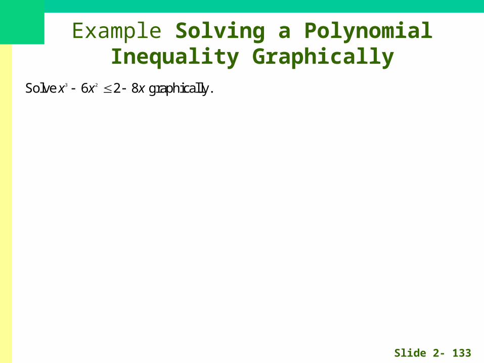
Example Solving a Polynomial Inequality Graphically
3 2Solve 6 2 8 graphically.x x x
Slide 2- 133
Example Solving a Polynomial Inequality Graphically
3 2Solve 6 2 8 graphically.x x x
3 2 3 2Rewrite the inequality 6 8 2 0. Let ( ) 6 8 2
and find the real zeros of graphically.
x x x f x x x x
f
The three real zeros are approximately 0.32, 1.46, and 4.21. The solution
consists of the values for which the graph is on or below the -axis.
The solution is ( ,0.32] [1.46,4.21].
x x

Slide 2- 134
Example Creating a Sign Chart for a Rational Function
1
Let ( ) . Determine the values of that cause ( ) to be3 1
(a) zero, (b) undefined, (c) positive, and (d) negative.
xr x x r x
x x
(a) ( ) 0 when 1.
(b) ( ) is undefined when 3 and 1.
r x x
r x x x
-3 1
(-)(-)(-)
negative positivepositive -1
(-)(+)(-)
(+)(+)(+)
(+)(+)(-)
negative
0und.und.
(c) ( 3, 1) (1, )
(d) ( , 3) ( 1,1)
0 und.

Slide 2- 135
Example Solving an Inequality Involving a Radical
Solve ( 2) 1 0.x x
Let ( ) ( 2) 1. Because of the factor 1, ( ) is undefined if
-1. The zeros are at -1 and 2.
f x x x x f x
x x x
-1 2
(-)(+) (+)(+)
undefined positivenegative
00
( ) 0 over the interval [ 1,2].f x

Slide 2- 136
Chapter Test
1. Write an equation for the linear function satisfying the given condition:
( 3) 2 and (4) 9.
2. Write an equation for the quadratic function whose graph contains the
vertex ( 2, 3) and the point
f
f f
(1,2).
3. Write the statement as a power function equation. Let be the constant
of variation. The surface area of a sphere varies directly as the square of
the radius .
4. Divide ( ) by ( ), an
k
S
r
f x d x3 2
d write a summary statement in polynomial form:
( ) 2 7 4 5; ( ) 3
5. Use the Rational Zeros Theorem to write a list of all potential rational
zeros. Then determine which ones, if any, are zero
f x x x x d x x
4 3 2
s.
( ) 2 4 6f x x x x x

Slide 2- 137
Chapter Test
4 3 2
3 2
2
6. Find all zeros of the function. ( ) 10 23
7. Find all zeros and write a linear factorization of the function.
( ) 5 24 12
8. Find the asymptotes and intercepts of the function.
( )
f x x x x
f x x x x
xf x
2
1
19. Solve the equation or inequality algebraically.
122 11
x
x
xx

Slide 2- 138
Chapter Test
10. Larry uses a slingshot to launch a rock straight up from a point
6 ft above level ground with an initial velocity of 170 ft/sec.
(a) Find an equation that models the height of the rock
seconds aft
t
er it is launched.
(b) What is the maximum height of the rock?
(c) When will it reach that height?
(d) When will the rock hit the ground?

Slide 2- 139
Chapter Test Solutions
1. Write an equation for the linear function satisfying the given condition:
( 3) 2 and (4) 9.
2. Write an equation for the quadratic function whose graph contains the
vertex ( 2, 3
5
) a
nd
f
f f y x
2 the point (1,2).
3. Write the statement as a power function equation. Let be the constant
of variation. The surface area of a sphere varies directly as the square of
the radi
5 / 9( 2
us
3
)
.
k
r
x
S
y
3 2
2
2
4. Divide ( ) by ( ), and write a summary statement in polynomial form:
( ) 2 7 4 5; ( ) 3
5. Use the Rational Zeros Theorem to write a list of all potential ration
2 2 1
3
f x d x
f x x x x
s kr
x xx
d x x
4 3 2
al
zeros. Then determine which ones, if any, are zeros.
( 1, 2, 3, 6 1/ 2, 3 / 2; 3 / 2 an) 2 4 d 26 f x x x x x

Slide 2- 140
Chapter Test Solutions
4 3 2
3 2
6. Find all zeros of the function. ( ) 10 23
7. Find all zeros and write a linear factorization of the function.
( ) 5 24 12
8. Find the asymptotes and in
0,5 2
4
tercepts
/ 5, 2 7
of
f x x x x
f x x x x
2
2-intercept (0,1), -intercept none
Vertical Asymptote 1, 1, H
the function.
1( )
1
9. Solve the equation or inequality
orizontal Asymptote
algebraically.
122
1
3/ 2 or 411
x xy x
x x
fx
xx x
x
x
y
Slide 2- 141
Chapter Test Solutions
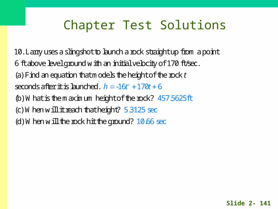
10. Larry uses a slingshot to launch a rock straight up from a point
6 ft above level ground with an initial velocity of 170 ft/sec.
(a) Find an equation that models the height of the rock
seconds aft
t2er it is launched.
(b) What is the maximum height of the rock?
(c)
-16 170 6
457.5625ft
5.When will it reach that height?
(d) When will the rock hit the groun
3125
d?
sec
10.66 sec
h t t