Slide 1 Copyright © 2004 Pearson Education, Inc. Chapter 3 Probability 3-1 Overview 3-2 Fundamentals 3-3 Addition Rule 3-4 Multiplication Rule: Basics

Copyright © 2004 Pearson Education, Inc.

Slide 1Chapter 3Probability

3-1 Overview

3-2 Fundamentals

3-3 Addition Rule

3-4 Multiplication Rule: Basics

3-5 Multiplication Rule: Complements and Conditional Probability

3-6 Probabilities Through Simulations

3-7 Counting


Slide 2

Created by Tom Wegleitner, Centreville, Virginia

Section 3-1 & 3-2 Overview & Fundamentals


Slide 3Overview

Rare Event Rule for Inferential Statistics:

If, under a given assumption (such as a lottery being fair), the probability of a particular observed event (such as five consecutive lottery wins) is extremely small, we conclude that the assumption is probably not correct.


Slide 4

Definitions

Event

Any collection of results or outcomes of a procedure.

Simple Event

An outcome or an event that cannot be further broken down into simpler components.

Sample Space

Consists of all possible simple events. That is, the sample space consists of all outcomes that cannot be broken down any further.


Slide 5Notation for Probabilities

P - denotes a probability.

A, B, and C - denote specific events.

P (A) - denotes the probability of event A occurring.


Slide 6Basic Rules for

Computing ProbabilityRule 1: Relative Frequency Approximation of Probability

Conduct (or observe) a procedure a large number of times, and count the number of times event A actually occurs. Based on these actual results, P(A) is estimated as follows:

P(A) = number of times A occurred

number of times trial was repeated



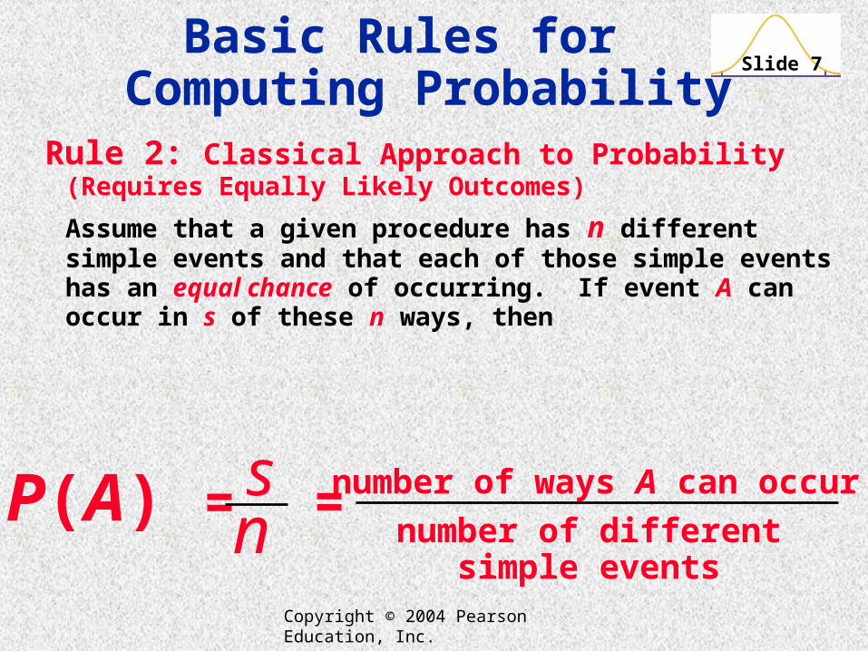
Computing ProbabilityRule 2: Classical Approach to Probability (Requires

Equally Likely Outcomes)

Assume that a given procedure has n different simple events and that each of those simple events has an equal chance of occurring. If event A can occur in s of these n ways, then

P(A) = number of ways A can occur

number of different simple events

sn =



Computing Probability

Rule 3: Subjective Probabilities

P(A), the probability of event A, is found by

simply guessing or estimating its value

based on knowledge of the relevant

circumstances.


Slide 9Law of Large Numbers

As a procedure is repeated again and again, the relative frequency probability (from Rule 1) of an event tends to approach the actual probability.


Slide 10Example

Roulette You plan to bet on number 13 on the next spin of a roulette wheel. What is the probability that you will lose?

Solution A roulette wheel has 38 different slots, only one of which is the number 13. A roulette wheel is designed so that the 38 slots are equally likely. Among these 38 slots, there are 37 that result in a loss. Because the sample space includes equally likely outcomes, we use the classical approach (Rule 2) to get

P(loss) = 37

38


Slide 11Probability Limits

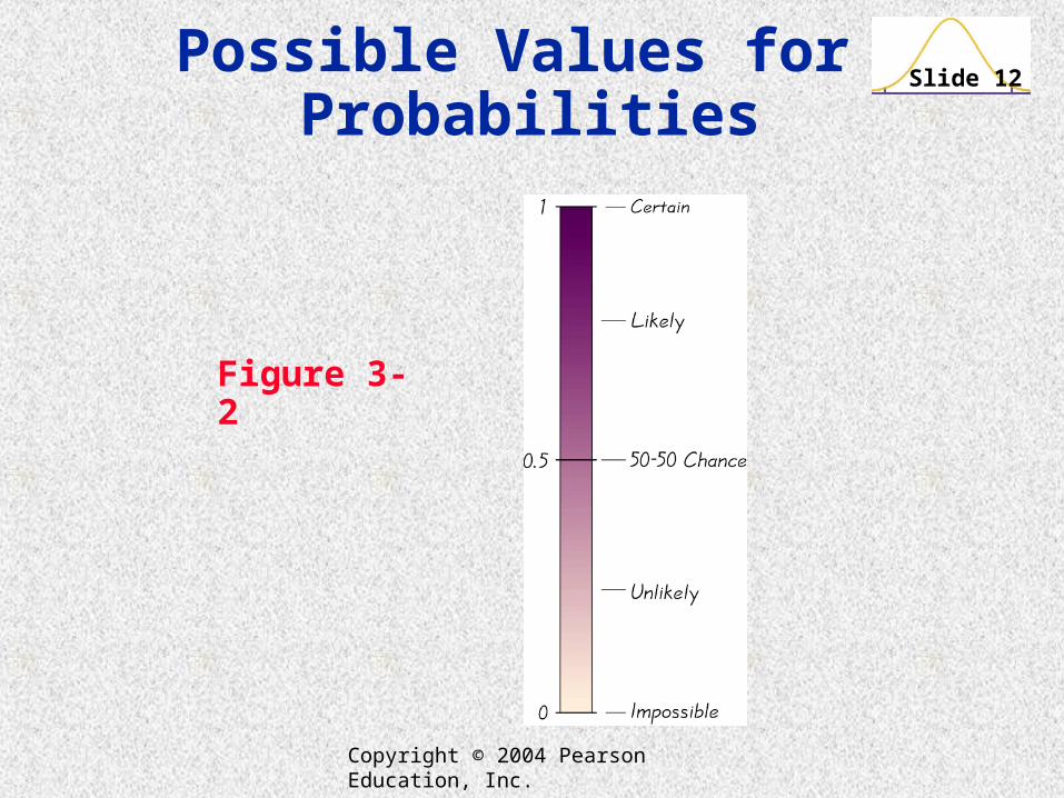
The probability of an event that is certain to occur is 1.

The probability of an impossible event is 0.

0 P(A) 1 for any event A.


Slide 12Possible Values for

Probabilities

Figure 3-2


Slide 13Definition

The complement of event A, denoted by A, consists of all outcomes in which the event A does not occur.


Slide 14

Example

Birth Genders In reality, more boys are born than girls. In one typical group, there are 205 newborn babies, 105 of whom are boys. If one baby is randomly selected from the group, what is the probability that the baby is not a boy?

Solution Because 105 of the 205 babies are boys, it follows that 100 of them are girls, so

P(not selecting a boy) = P(boy) = P(girl) 100

0.488205


Slide 15Definitions The actual odds against event A occurring are the ratio

P(A)/P(A), usually expressed in the form of a:b (or “a to b”), where a and b are integers having no common factors.

The actual odds in favor event A occurring are the reciprocal of the actual odds against the event. If the odds against A are a:b, then the odds in favor of A are b:a.

The payoff odds against event A represent the ratio of the net profit (if you win) to the amount bet.

payoff odds against event A = (net profit) : (amount bet)


Slide 16Recap

In this section we have discussed:

Rare event rule for inferential statistics.

Probability rules.

Law of large numbers.

Complementary events.

Rounding off probabilities.

Odds.


Slide 17


Section 3-3 Addition Rule


Slide 18

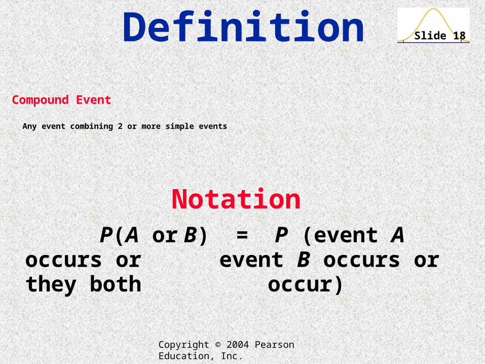
Compound Event

Any event combining 2 or more simple events

Definition

Notation

P(A or B) = P (event A occurs or event B occurs or they both

occur)


Slide 19

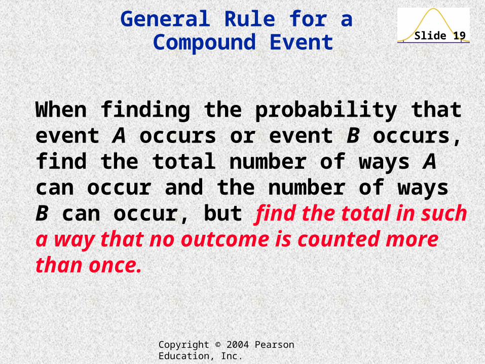
When finding the probability that event A occurs or event B occurs, find the total number of ways A can occur and the number of ways B can occur, but find the total in such a way that no outcome is counted more than once.

General Rule for a Compound Event


Slide 20Compound Event

Intuitive Addition Rule

To find P(A or B), find the sum of the number of ways event A can occur and the number of ways event B can occur, adding in such a way that every outcome is counted only once. P(A or B) is equal to that sum, divided by the total number of outcomes. In the sample space.

Formal Addition Rule

P(A or B) = P(A) + P(B) – P(A and B)

where P(A and B) denotes the probability that A and B both occur at the same time as an outcome in a trial or procedure.


Slide 21Definition

Figures 3-4 and 3-5

Events A and B are disjoint (or mutually exclusive) if they cannot both occur together.


Slide 22Applying the Addition Rule

Figure 3-6


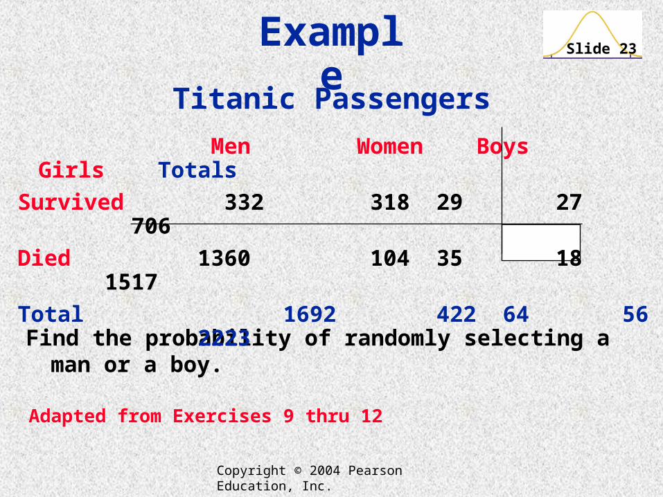
Slide 23

Find the probability of randomly selecting a man or a boy.

Titanic Passengers

Men Women Boys Girls Totals

Survived 332 318 29 27 706

Died 1360 104 35 18 1517

Total 1692 422 64 56 2223

Adapted from Exercises 9 thru 12

Example


Slide 24

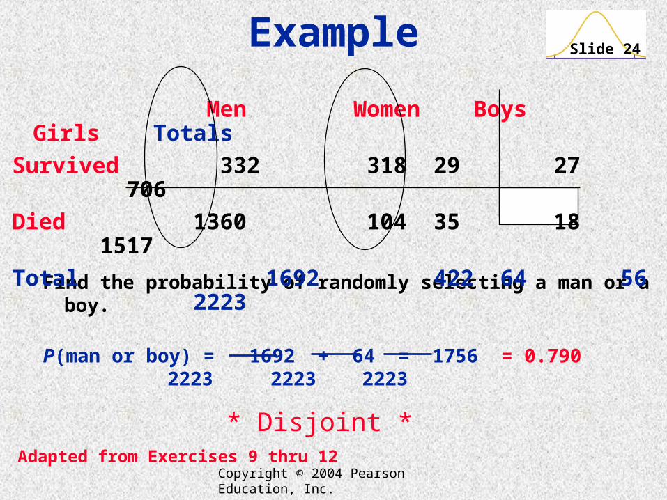
Find the probability of randomly selecting a man or a boy.

P(man or boy) = 1692 + 64 = 1756 = 0.790 2223 2223 2223


Survived 332 318 29 27 706

Died 1360 104 35 18 1517

Total 1692 422 64 56 2223

* Disjoint *

Example



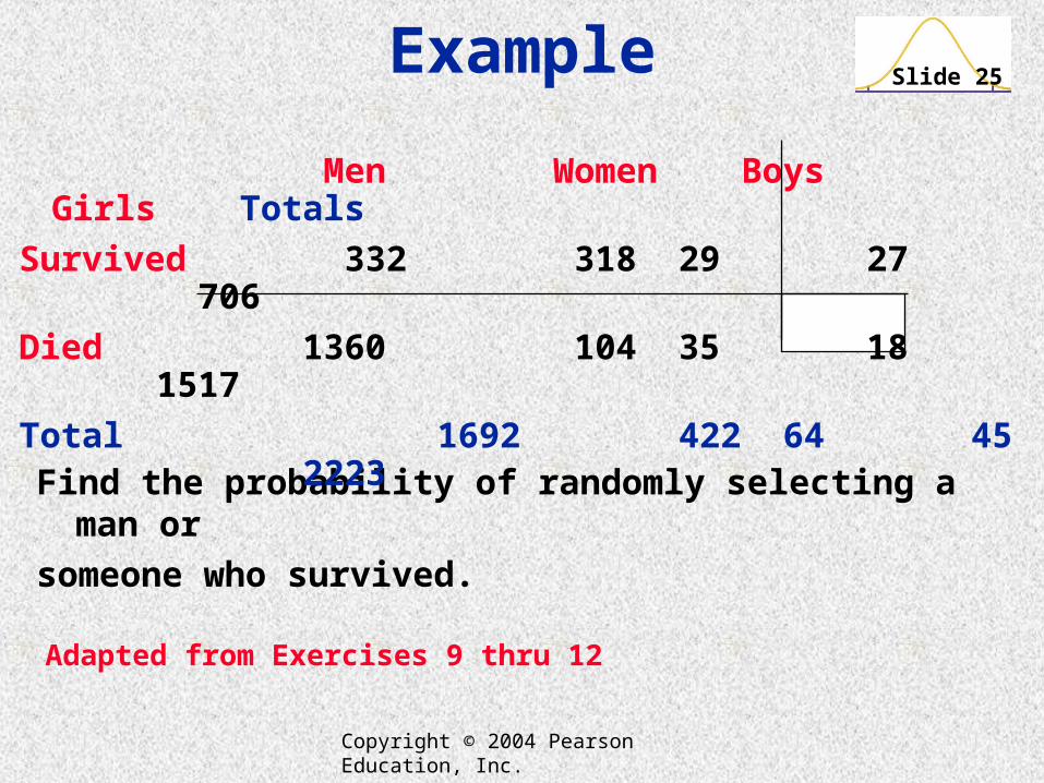
Slide 25

Find the probability of randomly selecting a man or

someone who survived.


Survived 332 318 29 27 706

Died 1360 104 35 18 1517

Total 1692 422 64 45 2223

Example



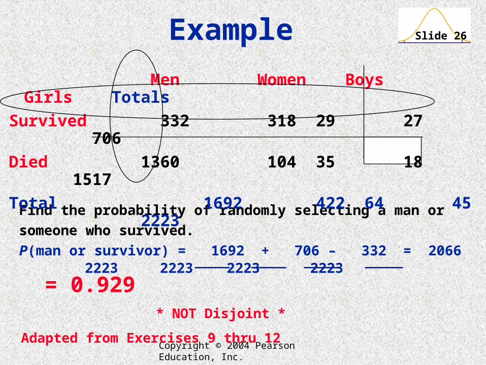
Slide 26

Find the probability of randomly selecting a man or

someone who survived.

P(man or survivor) = 1692 + 706 – 332 = 2066 2223 2223 2223 2223


Survived 332 318 29 27 706

Died 1360 104 35 18 1517

Total 1692 422 64 45 2223

* NOT Disjoint *

= 0.929


Example


Slide 27Complementary

Events

P(A) and P(A)are

mutually exclusive

All simple events are either in A or A.


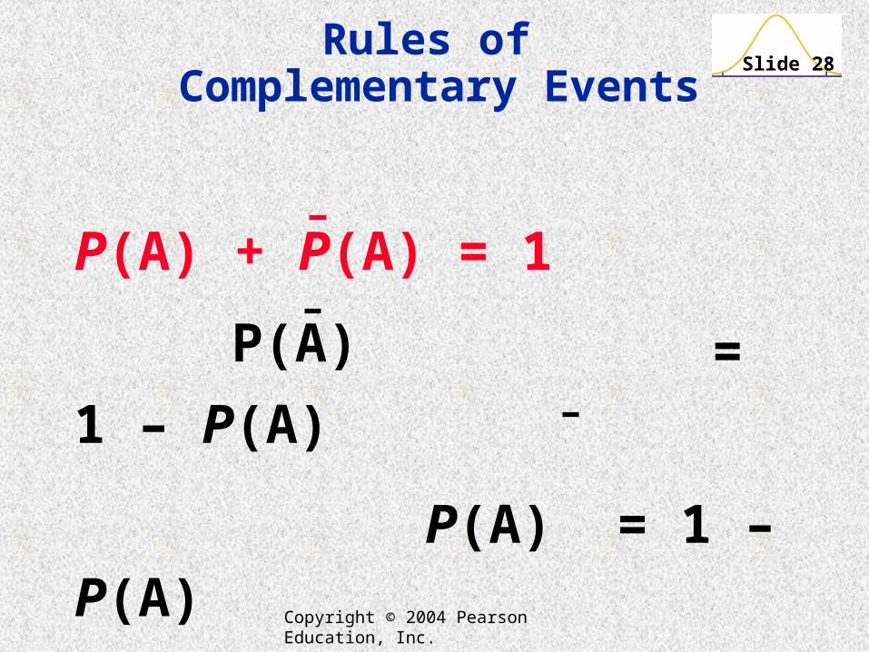
Slide 28

P(A) + P(A) = 1

= 1 – P(A)

P(A) = 1 – P(A)

P(A)

Rules of Complementary Events


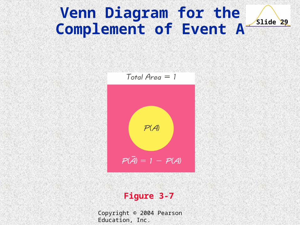
Slide 29Venn Diagram for the

Complement of Event A

Figure 3-7


Slide 30

Recap


Compound events.

Formal addition rule.

Intuitive addition rule.

Disjoint Events.

Complementary events.


Slide 31


Section 3-4 Multiplication Rule:

Basics


Slide 32Notation

P(A and B) =

P(event A occurs in a first trial and

event B occurs in a second trial)


Slide 33Tree DiagramsA tree diagram is a picture of the possible outcomes of a procedure, shown as line segments emanating from one starting point. These diagrams are helpful in counting the number of possible outcomes if the number of possibilities is not too large.

Figure 3-8 summarizes

the possible outcomes

for a true/false followed

by a multiple choice question.

Note that there are 10 possible combinations.


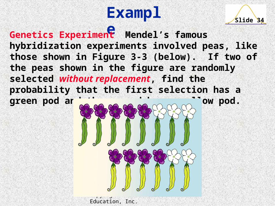
Slide 34Example

Genetics Experiment Mendel’s famous hybridization experiments involved peas, like those shown in Figure 3-3 (below). If two of the peas shown in the figure are randomly selected without replacement, find the probability that the first selection has a green pod and the second has a yellow pod.


Slide 35Example - Solution

First selection: P(green pod) = 8/14 (14 peas, 8 of which have green pods)

Second selection: P(yellow pod) = 6/13 (13 peas remaining, 6 of which have yellow pods)

With P(first pea with green pod) = 8/14 and P(second pea with yellow pod) = 6/13, we have

P( First pea with green pod and second pea with yellow pod) =

8 60.264

14 13


Slide 36Example

Important Principle

The preceding example illustrates the important principle that the probability for the second event B should take into account the fact that the first event A has already occurred.


Slide 37Notation for Conditional Probability

P(B A) represents the probability of event B occurring after it is assumed that event A has already occurred (read B A as “B given A.”)


Slide 38Definitions

Independent Events

Two events A and B are independent if the occurrence of one does not affect the probability of the occurrence of the other. (Several events are similarly independent if the occurrence of any does not affect the occurrence of the others.) If A and B are not independent, they are said to be dependent.


Slide 39Formal

Multiplication Rule

P(A and B) = P(A) • P(B A)

Note that if A and B are independent events, P(B A) is really the same

as P(B)


Slide 40Intuitive

Multiplication Rule

When finding the probability that event A occurs in one trial and B occurs in the next trial, multiply the probability of event A by the probability of event B, but be sure that the probability of event B takes into account the previous occurrence of event A.


Slide 41Applying the

Multiplication Rule

Figure 3-9


Slide 42Small Samples from

Large Populations

If a sample size is no more than 5% of the size of the population, treat the selections as being independent (even if the selections are made without replacement, so they are technically dependent).


Slide 43Summary of Fundamentals

In the addition rule, the word “or” on P(A or B) suggests addition. Add P(A) and P(B), being careful to add in such a way that every outcome is counted only once.

In the multiplication rule, the word “and” in P(A and B) suggests multiplication. Multiply P(A) and P(B), but be sure that the probability of event B takes into account the previous occurrence of event A.


Slide 44Recap


Notation for P(A and B).

Notation for conditional probability.

Independent events.

Formal and intuitive multiplication rules.

Tree diagrams.


Slide 45


Section 3-5 Multiplication Rule:Complements and

Conditional Probability


Slide 46Complements: The Probability

of “At Least One”

The complement of getting at least one item of a particular type is that you

get no items of that type.

“At least one” is equivalent to “one or more.”


Slide 47Example

Gender of Children Find the probability of a couple having at least 1 girl among 3 children. Assume that boys and girls are equally likely and that the gender of a child is independent of the gender of any brothers or sisters.

Solution

Step 1: Use a symbol to represent the event desired. In this case, let A = at least 1 of the 3 children is a girl.


Slide 48

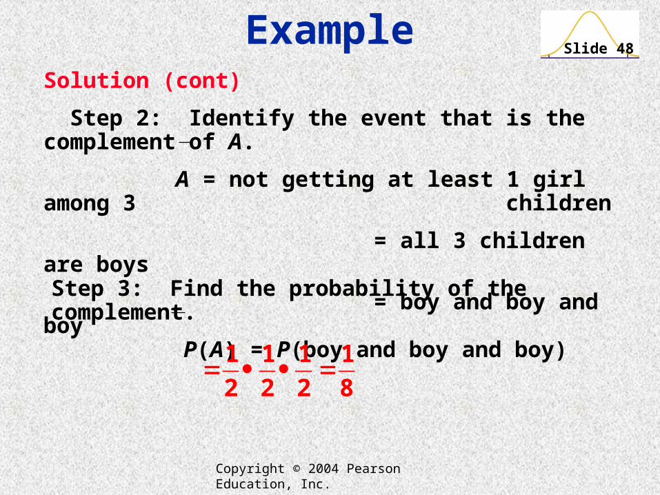
Solution (cont)

Step 2: Identify the event that is the complement of A.

A = not getting at least 1 girl among 3 children

= all 3 children are boys

= boy and boy and boy

Example

Step 3: Find the probability of the complement.

P(A) = P(boy and boy and boy)

1 1 1 1

2 2 2 8


Slide 49Example

Solution (cont)

Step 4: Find P(A) by evaluating 1 – P(A).

1 7( ) 1 ( ) 1

8 8 P A P A

Interpretation There is a 7/8 probability that if a couple has 3 children, at least 1 of them is a girl.


Slide 50Key Principle

To find the probability of at least one of something, calculate the probability of none, then subtract that result from 1. That is,

P(at least one) = 1 – P(none)


Slide 51Definition

A conditional probability of an event is a probability obtained with the additional information that some other event has already occurred. P(B A) denotes the conditional probability of event B occurring, given that A has already occurred, and it can be found by dividing the probability of events A and B both occurring by the probability of event A:

P(B A) = P(A and B)

P(A)


Slide 52Intuitive Approach to

Conditional Probability

The conditional probability of B given A can be found by assuming that event A has occurred and, working under that assumption, calculating the probability that event B will occur.


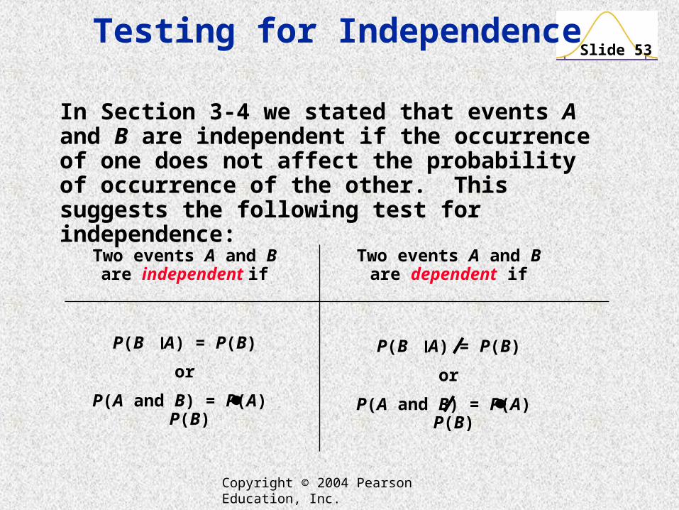
Slide 53Testing for Independence

In Section 3-4 we stated that events A and B are independent if the occurrence of one does not affect the probability of occurrence of the other. This suggests the following test for independence:

Two events A and B are independent if

Two events A and B are dependent if

P(B A) = P(B)

or

P(A and B) = P(A) P(B)

P(B A) = P(B)

or

P(A and B) = P(A) P(B)


Slide 54Recap


Concept of “at least one.”

Conditional probability.

Intuitive approach to conditional probability.

Testing for independence.


Slide 55


Section 3-6Probabilities Through

Simulations


Slide 56Definition

A simulation of a procedure is a process that behaves the same way as the procedure, so that similar results are produced.


Slide 57Simulation Example

Gender Selection When testing techniques of gender selection, medical researchers need to know probability values of different outcomes, such as the probability of getting at least 60 girls among 100 children. Assuming that male and female births are equally likely, describe a simulation that results in genders of 100 newborn babies.


Slide 58Simulation Examples

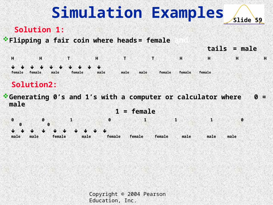
Solution 1:

Flipping a fair coin where heads = female and

tails = maleH H T H T T H H H H female female male female male male male female female female


Slide 59Simulation Examples

Solution 1:Flipping a fair coin where heads = female and

tails = maleH H T H T T H H H H female female male female male male male female female female

Solution2:

Generating 0’s and 1’s with a computer or calculator where 0 = male 1 = female0 0 1 0 1 1 1 0 0 0

male male female male female female female male male male


Slide 60Random Numbers

In many experiments, random numbers are used in the simulation naturally occurring events. Below are some ways to generate random numbers.

A random table of digits

Minitab

Excel

TI-83 Plus calculator

STATDISK


Slide 61Recap


The definition of a simulation.

Ways to generate random numbers.

How to create a simulation.


Slide 62


Section 3-7Counting


Slide 63Fundamental Counting Rule

For a sequence of two events in which the first event can occur m ways and the second event can occur n ways, the events together can occur a total of m n ways.


Slide 64Notation

The factorial symbol ! Denotes the product of decreasing positive whole numbers. For example,

4! 4 3 2 1 24.

By special definition, 0! = 1.


Slide 65

A collection of n different items can be arranged in order n! different ways. (This factorial rule reflects the fact that the first item may be selected in n different ways, the second item may be selected in n – 1 ways, and so on.)

Factorial Rule


Slide 66

Permutations Rule(when items are all different)

(n - r)!n rP = n!

The number of permutations (or sequences) of r items selected from n available items (without replacement is


Slide 67Permutation Rule:

Conditions

We must have a total of n different items available. (This rule does not apply if some items are identical to others.)

We must select r of the n items (without replacement.)

We must consider rearrangements of the same items to be different sequences.


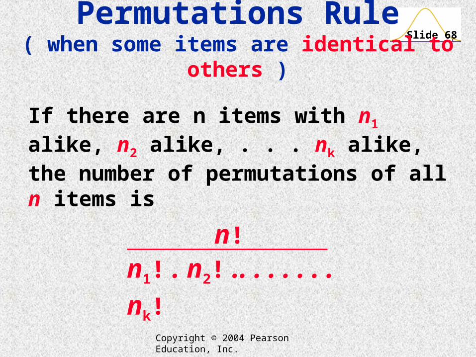
Slide 68Permutations Rule( when some items are identical to others )

n1! . n2! .. . . . . . . nk! n!

If there are n items with n1 alike, n2 alike, . . . nk alike, the number of permutations of all n items is


Slide 69

(n - r )! r!n!

nCr =

Combinations Rule

The number of combinations of r items selected from n different items is


Slide 70Combinations Rule:

Conditions

We must have a total of n different items available.

We must select r of the n items (without replacement.)

We must consider rearrangements of the same items to be the same. (The

combination ABC is the same as CBA.)


Slide 71

When different orderings of the same items are to be counted separately, we have a permutation problem, but when different orderings are not to be counted separately, we have a combination problem.

Permutations versus Combinations


Slide 72Recap


The fundamental counting rule.

The permutations rule (when items are all different.)

The permutations rule (when some items are identical to others.)

The combinations rule.

The factorial rule.

Documents

Slide 1 Copyright © 2004 Pearson Education, Inc. Chapter 3 Probability 3-1 Overview 3-2 Fundamentals 3-3 Addition Rule 3-4 Multiplication Rule: Basics