SLAC{PUB{7215

December 1996

A Topological Vertex Reconstruction Algorithm for HadronicJets�

David J. Jackson

Stanford Linear Accelerator Center,

Stanford University, Stanford, CA 94309

Permanent address: Rutherford Appleton Laboratory,

Chilton, Didcot, Oxfordshire OX11 0QX, England

E-mail: djackson@slac.stanford.edu

Abstract

The algorithm described reconstructs a set of topological vertices each

associated with an independent subset of the charged tracks in a hadronic

jet. Vertices are reconstructed by associating tracks with 3D spatial regions

according to a vertex probability function which is based on the trajectories

and position resolution of the tracks. SLD data is used to illustrate the

performance of the algorithm with emphasis on the application to Z0 ! bb

events.

To appear in Nuclear Instruments and Methods

�Work supported by the UK Particle Physics and Astronomy Research Council and

Department of Energy contract DE{AC03{76SF00515.

1 Introduction

A hadronic jet containing weakly decaying hadrons is composed of particles

with di�ering origins. A charged track may be produced at either the jet

origin, i.e. the primary vertex, or at a hadronic decay vertex. If the spatial

separation of the true vertices is not signi�cantly greater than the tracking

resolution then the vertices are generally not easily identi�ed and ambigui-

ties arise in associating tracks with vertices. The technique described here

is designed to optimise the vertex reconstruction performance in such an

environment. This topological vertex �nding algorithm has been developed

for data collected by the SLC Large Detector (SLD) at the Stanford Linear

Collider (SLC). The excellent 3D resolution of the SLD pixel vertex detector

(VXD2) makes the e�cient reconstruction of decay vertices in the hadronic

jets produced by Z0 decays possible.

Figure 1: Tracks produced (solid lines) in one hemisphere of a Z0 ! bb event.

Since the mass of the Z0 is signi�cantly greater than the mass of the quark

pairs it can decay into, the events can be divided into two hemispheres. For

a Z0 ! bb event a B hadron decay is expected in each hemisphere (except

2

in the case of hard gluon radiation). Such a hemisphere from a Z0 ! bb

event is represented in �g. 1. In this case the tracks originate from three

vertices; the fragmentation tracks from the primary vertex at the e+e� IP

(Interaction Point), tracks from the secondary B hadron decay and tracks

from the tertiary D hadron decay. The reconstruction of vertices formed by

the tracks from the weakly decaying hadrons allow the properties of such

hadrons to be studied.

The decay lengths are typically shorter than the distance to the �rst layer

of the vertex detector. Hence no information about the location of the track

origin longitudinal to the trajectory is measured, while the transverse position

is measured to within the resolution of the vertex detector. In other words

there is some degree of uncertainty concerning the transverse origin of each

track while the longitudinal origin of the track is completely undetermined.

However, by combining the tracking information for the set of tracks in the

jet the topological vertex structure may be identi�ed. The following section

describes this procedure.

2 An Algorithm to Resolve Vertices

The philosophy adopted is to search for vertices in 3D co-ordinate space

rather than by forming vertices from all track combinations (the latter be-

comes impracticable for events with high track multiplicity). This search is

based on a function V (r) which quanti�es the relative probability of a vertex

at location r. The �rst step is to obtain from the helix parameters (or, in

general, the relevant trajectory parameters) of each track i a function fi(r)

representing a Gaussian probability tube for the track trajectory,

fi(r) = exp

8<:�1

2

24 x0 � (x00 + �y0

2

)

�T

!2+

z � (z0 + tan(�)y0)

�L

!2359=; ; (1)

where the x; y co-ordinates have been transformed into x0; y0 for each track

such that the track momentum is parallel to the positive y0 co-ordinate axis

in the xy plane at the point of closest approach to the IP (x00; z0 are the

x0; z co-ordinates at this point). The Gaussian tube is represented by the

3

parallel dotted lines in �g. 2. The �rst term inside the exponential includes

a parabolic approximation to the circular track trajectory in the xy plane,

where � is determined from the magnetic �eld and the particle charge and

transverse momentum. The trajectory is propagated into the third dimension

z via the helix parameter � in the second term of the exponential. The

quantities �T and �L are the measurement errors for the track in the xy

plane and z direction respectively. In general these quantities are a function

of location since the track trajectory is known more precisely close to a hit in

the vertex detector. If the distance to the �rst layer of the vertex detector is

large compared with the region of physics interest close to the IP then �T and

�L may be treated as constants, measured at the point of closest approach

of the track to the IP.

Figure 2: Construction of the Gaussian tube fi(r) for each track i.

In order ultimately to decide which of the vertices is the primary and to

constrain it to be consistent with the IP position a further function f0(r) is

introduced describing the IP location and uncertainty. For SLD it is simply

a 3D unnormalized Gaussian ellipsoid centred on the IP with �X = �Y =

4

7�m and �Z=70�m re ecting the uncertainty in the position of the IP (see

section 5.1). The IP function is analogous to fi(r) for the tracks and it

is treated in a similar way. The notation `track-IP' will be used when a

statement refers to both the track and the IP functions. The weight given

to f0(r) in calculating V (r) may be modi�ed by a tunable parameter (see

section 4). Using the function f0(r) improves the vertex �nding performance

by introducing information additional to that contained in the jet of tracks

being considered (see section 5.1).

The Gaussian track functions are left unnormalized in order that the ver-

tex function introduced below is sensitive to track multiplicity as a function

of r. The relative probability of a vertex at r is de�ned taking into account

that the value of fi(r) must be signi�cant for at least two tracks-IP in this

region. A smooth, continuous function is desired so that its maxima may be

found. These requirements result in the form:

V (r) =NXi=0

fi(r)�

PNi=0 f

2

i (r)PNi=0 fi(r)

: (2)

where N is the number of tracks. The �rst term on the rhs is a measure

of the multiplicity and degree of overlap of the track-IP probability functions

and hence a measure of the probability that at least some of the tracks

originate at r and hence form a vertex at this location. Due to the second

term on the rhs of equation 2, V (r) ' 0 in regions where fi(r) is signi�cant

for only one track-IP. The form of V (r) can be modi�ed to fold in known

physics information about probable vertex locations (see section 4).

An example of the xy projection ofPN

i=0 fi(r) and V (r) is shown in

�g. 3(a) and 3(b) respectively. These plots are obtained by integrating the

function over the third dimension z within the limits of �0:8 cm from the

IP in the z direction. (This 2D projection is for diagrammatic convenience

only). The hemisphere of tracks chosen for this plot is taken from an SLD

Monte Carlo Z ! bb event in which the jet momentum is directed from left

to right in �g. 3. The trajectories of individual tracks can be seen in �g. 3(a).

The regions where vertices are probable can be seen from the distribution of

V (r) in �g. 3(b). In this case the algorithm resolved the hemisphere into two

vertices, i.e. the primary vertex and a secondary. The peak in V (r) produced

by the primary can be seen in �g. 3(b) at X =Y =0, the secondary peak is

displaced to the right of the IP by � 0:15 cm. A subset of the tracks-IP is

5

Figure 3: The track (a) and vertex (b) functions projected onto the xy plane

(cm).

associated with each of the resolved maxima of V (r) to identify the set of

reconstructed vertices.

Figure 4: Reconstruction of heavy hadron decay lengths in Z0 ! bb events.

Fig. 4 shows the reconstructed decay lengths from SLD Z0 ! bb Monte

Carlo hemispheres for (a) the B hadron decay length in which one secondary

vertex has been found, and (b) the D decay length in events for which a ter-

tiary vertex is also reconstructed. The asymmetry of the scatter plot about

the diagonal in �g. 4(a) is the e�ect of the cascade charm decay augmenting

6

the reconstructed B decay length. To fully reconstruct the B to D decay

chain for �g. 4(b) requires at least two charged tracks to be well measured

from both hadron decays and that all three vertices (including the primary)

be well separated, the e�ciency and purity of the full reconstruction is there-

fore somewhat lower than that for �nding a single displaced vertex. However,

the algorithm will attempt to fully reconstruct all physics vertices in the jet

of tracks. A vertex can be reconstructed if it is spatially `resolved' from other

vertices.

The criterion used for resolving maxima of V (r) is the following, it is

used wherever terms like `resolved' appear in this paper. The two locations

r1 and r2 are said to be resolved if:

minfV (r) : r 2 r1 + �(r2 � r1); 0 � � � 1g

minfV (r1); V (r2)g< R0; (3)

where minfV (r1); V (r2)g is the lower of the two values and the numerator

in equation 3 is the minimum of V (r) on a straight line joining r1 and r2; in

practice V (r) is determined for a �nite number of points on this line. The

number of vertices found will depend on the cut value, 0 � R0 � 1, chosen.

The value of R0 as well as the maximum �2 contribution of a track to a

vertex, �20 (discussed below), are tunable parameters.

It is not necessary to search the whole of the 3D space in the region of

physics interest in order to �nd the maxima of V (r). Since at least two

of the functions fi(r) must contribute to a maximum in V (r) the spatial

locations of the maxima of fi(r)fj(r) are �rst found by direct calculation.

For each of these spatial points the corresponding 3D maximum is found in

V (r) iteratively in the proximity of the fi(r)fj(r) maximum. By initializing

this iterative procedure at the calculated maxima of fi(r)fj(r) the e�ective

3D search area is much smaller than the potential region of physics vertices

and all the maxima in V (r) are found. These maxima are clustered together

to form candidate vertex regions using the resolution criterion. If a maximum

in V (r) which was found near the maximum of fi(r)fj(r) is included in such a

cluster, then the tracks i and j belong to the corresponding vertex candidate.

If the IP function (i = 0) is included in the cluster then the vertex is identi�ed

as the primary. This procedure is described in more detail in the following

paragraphs.

In a jet of N tracks the 1

2N(N +1) locations rij of the fi(r)fj(r) maxima

(i; j = 0 . . .N; i 6= j) are found and retained if both tracks-IP pass the cut

7

�2 < �20 at rij. The track-IP k is associated with the spatial point having

the greatest value of V (rkj) (obtained for j = 0 . . . k�1; k+1 . . .N). In addi-

tion, for each track, in order of decreasing values of V (rkj) further locations

are retained in association with the track if they are resolved from locations

already associated with the track. The resolution criterion is used here since

there is no need to associate a track with two spatial points that will ulti-

mately be clustered into the same vertex region. In general each track may

therefore be associated with 0 to N spatial locations although in practice this

number is much less than N . Allowing the tracks to be associated with more

than one spatial region enhances the vertex �nding e�ciency; it also leads

to ambiguities in assigning a track to a unique vertex which must later be

resolved. The IP is associated with only one spatial point (i.e. the location

of the highest V (r0j)).

An iterative procedure in xyz space transforms each of the rij (maxima

of fi(r)fj(r)) into the location of the nearest maximum in V (r). The trans-

formed spatial points rij are then clustered into separate regions of 3D space

according to the resolution criterion. The spatial point with the highest

V (rij) is taken as the seed of the �rst cluster. All spatial points not resolved

from this seed location according to equation 3 are added to the cluster. Any

remaining spatial points are added to the cluster if they are not resolved from

any spatial point in the cluster; this procedure continues until no further lo-

cations are added to the cluster. Of the remaining unclustered spatial points

the one with the highest V (rij) is now taken as the seed of the second cluster

and the above procedure is repeated. This clustering algorithm of taking

a seed location and adding unresolved locations continues until no spatial

points remain unclustered. The resulting number of clusters (typically � 4

for a jet at SLD in which a B hadron decays at > 0:1 cm) is equal to the

number of candidate vertices in the jet.

The candidate vertices are formed by associating the resolved spatial

clusters with a subset of the N tracks and the IP via the set spatial points

rij forming the cluster. Since the tracks were allowed to be associated with

several resolved spatial points the subsets of tracks associated with the spatial

cluster will in general not be independent. At all stages non-primary vertices

are rejected if they consist of < 2 tracks (by de�nition). The subset of tracks

in each vertex is taken in turn and �t to a common vertex. If the track with

the largest �2 contribution to the vertex fails the cut �2 < �20 it is removed

from the vertex, and the remaining tracks (if � 2) are re�t. The process

8

is repeated iteratively until all tracks with a bad �2 contribution have been

trimmed away. The �t is not explicitly checked in the clustering process

and the �2 trimming avoids vertices in the �nal set having a very low �t

probability. Any remaining track ambiguities are decided as follows. The

tracks in the vertex with the largest value of V (r) (taken to be the highest

V (rij) in the spatial cluster forming the vertex) are �xed in that vertex and

removed from any others. The remaining vertices are considered in order

of decreasing values of V (r) and at each stage the tracks still remaining in

the vertex are �xed into that vertex and removed from vertices with smaller

V (r) values. This procedure uniquely assigns each track to a vertex, each of

which is re�t and the topological vertex �nding is complete. (Alternatively, it

may be desirable to retain a degree of ambiguity and associate tracks with an

arbitrary number of vertices with each association being characterized by the

corresponding �2 contribution of the track to the vertex). The vertex found

to include the IP function is called the primary vertex and may be associated

with any number from 1 to N tracks. If the IP does not belong to any of

the resolved spatial clusters then there are no tracks in the primary vertex.

The non-primary vertices are labelled (secondary, tertiary etc.) according to

their distance from the IP.

3 Topological track parameters

The information obtained for each track includes the associated vertex num-

ber (unassociated tracks are classi�ed as `isolated') and the �2 contribution

of the track to this vertex. Topological track parameters are de�ned and

measured as follows. A vertex axis is formed by a straight line joining the IP

to a secondary (seed) vertex, �g. 5. If several non-primary vertices are found

one must be selected as the seed vertex. For example, the most signi�cant

vertex (highest value of V (r)) or the one reconstructed furthest from the IP

(used in this case) may be chosen as the seed. The transverse 3D impact

parameter, T, and the distance along the vertex axis to this point, L, are cal-

culated. Tracks classi�ed as isolated but having small values of T are likely to

be associated with the decay sequence in a Z0 ! bb event hemisphere (since

the momentum of the cascade D hadron is approximately collinear with the

9

Figure 5: Impact parameter of a track to the vertex axis.

momentum of the parent B hadron). The value of L for such tracks, com-

pared with the vertex decay length, D, locates the track position along the

decay chain. The quantity L/D is plotted in �g. 6 for tracks classi�ed as iso-

lated but of di�ering Monte Carlo origins. Hence these parameters allow the

possibility of reconstructing `one-prong vertices', (e.g. a lepton `vertex' in a

semileptonic B decay) relative to a topologically reconstructed multi-prong

vertex.

4 Tuning the Algorithm

In addition to R0, equation 3, and �20 two further tunable parameters, KIP

and K� are used to optimize the topological vertexing performance. The

10

Figure 6: The ratio L/D for tracks reconstructed as isolated in Z0 ! bb

Monte Carlo events for primary (solid line), B decay (dashed line) and D

decay (dotted line) tracks.

latter two parameters allow the vertex signi�cance function V (r) (equation 2)

to be weighted in regions where real vertices are more probable. In general,

V (r) may be given a high or low weight in regions where the genuine or fake

(respectively) vertex probability is expected to be high due to considerations

such as physics, kinematics or geometry. The weight KIP is introduced into

the de�nition of V (r):

V (r) = KIP f0(r) +NXi=1

fi(r)�KIP f

2

0 (r) +PN

i=1 f2

i (r)

KIP f0(r) +PN

i=1 fi(r): (4)

Values of KIP > (<) 1:0 mean that it is less (more) likely that secondary

vertices will be found near the IP, a region where the fake vertex background

is large. That is, large values of KIP will enhance V (r) at the IP and absorb

more tracks into the primary vertex. In addition, the vertex function may

be modi�ed by a factor dependent upon the angular location of the spatial

point r:

V (r)! V (r) exp(�K��2); (5)

where the angle � is de�ned in �g. 7. The dimensions used are suitable

for the SLD environment. The cylinder of radius 50 �m centred on the jet

11

Figure 7: Construction of �, the angular displacement.

axis is constructed in order that V (r) is not reduced in the area close to the

IP. In the regions where the distance from the IP projected onto the jet axis

is < �100�m or > 2:5cm, V (r) is set equal to zero since these locations are

unlikely to contain useful vertices. Fake vertices involving primary tracks

diverging from the IP are more likely to occur at higher values of � than the

genuine secondaries. By either a cut on the value of � for a vertex location

after the vertices have been found or tuning K� (� 5:0 for a 45 GeV jet

at SLD, in general K� should be proportional to the jet momentum) at the

input stage, the purity of the secondary vertices can be improved.

12

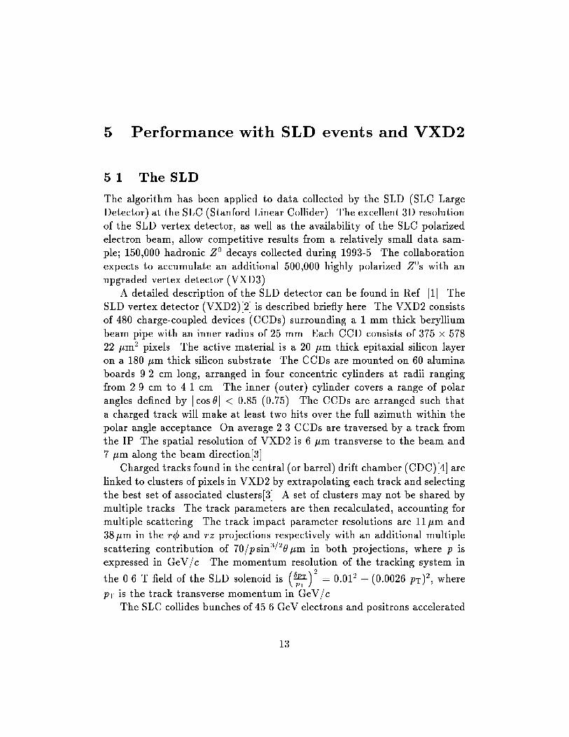
5 Performance with SLD events and VXD2

5.1 The SLD

The algorithm has been applied to data collected by the SLD (SLC Large

Detector) at the SLC (Stanford Linear Collider). The excellent 3D resolution

of the SLD vertex detector, as well as the availability of the SLC polarized

electron beam, allow competitive results from a relatively small data sam-

ple; 150,000 hadronic Z0 decays collected during 1993-5. The collaboration

expects to accumulate an additional 500,000 highly polarized Z0s with an

upgraded vertex detector (VXD3).

A detailed description of the SLD detector can be found in Ref. [1]. The

SLD vertex detector (VXD2)[2] is described brie y here. The VXD2 consists

of 480 charge-coupled devices (CCDs) surrounding a 1 mm thick beryllium

beam pipe with an inner radius of 25 mm. Each CCD consists of 375 � 578

22 �m2 pixels. The active material is a 20 �m thick epitaxial silicon layer

on a 180 �m thick silicon substrate. The CCDs are mounted on 60 alumina

boards 9.2 cm long, arranged in four concentric cylinders at radii ranging

from 2.9 cm to 4.1 cm. The inner (outer) cylinder covers a range of polar

angles de�ned by j cos �j < 0:85 (0:75). The CCDs are arranged such that

a charged track will make at least two hits over the full azimuth within the

polar angle acceptance. On average 2.3 CCDs are traversed by a track from

the IP. The spatial resolution of VXD2 is 6 �m transverse to the beam and

7 �m along the beam direction[3].

Charged tracks found in the central (or barrel) drift chamber (CDC)[4] are

linked to clusters of pixels in VXD2 by extrapolating each track and selecting

the best set of associated clusters[3]. A set of clusters may not be shared by

multiple tracks. The track parameters are then recalculated, accounting for

multiple scattering. The track impact parameter resolutions are 11�m and

38�m in the r� and rz projections respectively with an additional multiple

scattering contribution of 70=p sin3=2� �m in both projections, where p is

expressed in GeV/c. The momentum resolution of the tracking system in

the 0.6 T �eld of the SLD solenoid is��pTpT

�2= 0:012 + (0:0026 pT)

2, where

pT is the track transverse momentum in GeV/c.

The SLC collides bunches of 45.6 GeV electrons and positrons accelerated

13

in the SLAC linac at a rate of 120 Hz. The spatial extent of the bunches at

the IP is typically � 0:8 �m vertically, � 2:6 �m horizontally, and � 700 �m

longitudinally[5]. The transverse position of the SLC collision region is stable,

with variations of typically 5-10 �m over time periods measured in hours. A

�t to a single point in the transverse plane is made using tracks from � 30

successive hadronic Z0 decays to �nd the spatial location of the IP [3] with

an uncertainty of 7�2 �m. The median z position of tracks at their point of

closest approach to the IP in the xy plane is used to determine the z position

of the e+e� interaction on an event-by-event basis. A precision of � 52�m

on this quantity is estimated using Z0 ! bb Monte Carlo [3].

Figure 8: Vertex reconstruction in Monte Carlo Z0 ! bb event hemispheres

(a) e�ciency, (b) multiplicity (c) �t probability.

14

5.2 Vertexing Performance

Following standard SLD event and track selection the algorithm is applied

separately to the tracks in each event hemisphere. The tuning parameters

are set to R0 = 0:6, �20 = 10:0, KIP = 1:0, and K� = 5:0. Monte Carlo

events generated using JETSET 7.4 [6] with the SLD detector simulated

by GEANT 3.21 [7] are used to study the vertex �nding e�ciencies and

purities. The e�ciency for reconstructing a secondary vertex in a Z0 ! bb

event hemisphere is shown in �g. 8(a) as a function of the true B hadron

decay length. The e�ciency is lower for short B decay length since it becomes

harder to resolve the secondary, from the primary, near the IP. Larger value of

R0 (equation 3) increase the vertex �nding e�ciency in this region, at the cost

of purity. The vertex multiplicity is shown in �g. 8(b), where the `1 vertex'

case means that only the primary vertex was found. The total e�ciency

for reconstructing a secondary vertex in a Z0 ! bb event hemisphere is

about 50% (in charm and light quark hemispheres it is about 15% and 3%

respectively). The probability of the secondary vertex �t is shown in �g. 8(c).

The size of the peak near zero probability depends directly on the input value

of �20, the maximum �2 contribution of a track to a vertex. Otherwise the

probability spectrum is at, as expected for genuine vertices. The purity

of the vertices, that is the likelihood of correctly associating a track with a

vertex is shown in table 1 for the case in which a secondary only (two vertex

case) and a secondary plus tertiary (three vertex case) is reconstructed.

Monte Carlo Reconstructed track-vertex association

track origin Two vertex case Three vertex case

pri sec iso pri sec ter iso

Primary 93 3 4 77 16 3 4

B decay 14 80 6 6 65 25 4

D decay 8 82 10 3 25 68 4

Table 1: Purity of reconstructed track-vertex association (%).

As shown above (�g. 6) the isolated tracks may be attached to the seed

vertex via a cut on the quantity L/D. The selection of tracks resulting from

theB decay chain is optimized by attaching all non-seed tracks with L/D>0.3

15

Figure 9: Reconstructed secondary vertex mass for SLD 1994-5 data (points)

and Monte Carlo (solid line) composed of Z0 ! bb events (dashed lines),

Z0 ! cc events (dotted line) and light quark events (dash-dotted line) .

(including tracks initially classi�ed as primary). The invariant mass spectrum

of this set of tracks (tracks in the seed vertex or passing L/D>0.3) is shown in

�g. 9 for vertices reconstructed at a distance greater than 0.1cm from the IP.

The vertex mass is calculated by assuming that each track has the mass of a

pion. The Monte Carlo event sample used in this plot is 2.5 times larger than

the 1994-5 data sample. A K0

S mass peak is visible around 0.5 GeV/c2. For

the B and D decays the reconstructed mass is generally less than that of the

decaying hadron due to the missing neutral energy. The mass spectrum for

the Z0 ! cc events falls rapidly above theD hadron mass (around 2 GeV/c2)

leaving a purer sample of Z0 ! bb events which are reconstructed up to the B

hadron mass around 5 GeV/c2. This sample of vertices with mass > 2GeV/c2

has a high purity of tracks from the B decay chain such that the total charge

of these tracks tags neutral or charged B decays. This charge reconstruction

has been used at SLD to measure the ratio of the B0 and B+ lifetimes [8].

16

References

[1] SLD Design Report, SLAC-REPORT-273, May 1984.

[2] G.D. Agnew et al., \Design and Performance of the SLD Vertex Detector,

a 120 MPixel Tracking System", Proceedings of the XXVI International

Conference on High Energy Physics, Dallas, Texas, 6{12 August, 1992,

M. Strauss et al., \Performance of the SLD CCD Pixel Vertex Detector

and Design of an Upgrade," Proceedings of the 27th International Con-

ference on High Energy Physics, Glasgow, Scotland, July 20-27, 1994.

[3] K. Abe et al., \Measurements of Rb with Impact Parameters and Dis-

placed Vertices", Phys. Rev. D53, 1023 (1996).

[4] M.D. Hildreth et al., \Performance of the SLD Central Drift Chamber",

IEEE Trans. Nucl. Sci. 42, 451 (1995).

[5] M. Breidenbach, \SLC and SLD { Experimental Experience with a Linear

Collider", in Waikoloa 1993, Proceedings, Physics and Experiments with

Linear e+ e- Colliders, vol. 1, pp. 30-45, and SLAC-PUB-6313 (August

1993).

[6] T. Sj�ostrand, CERN-TH-7112-93, Feb. 1994.

[7] R. Brun et al., CERN-DD/EE/84-1, 1989.

[8] K. Abe et al., \Preliminary Measurements of B0 and B+ Lifetimes at

SLD", SLAC-PUB-6972, August 1995.

17