Skin Effect Sbs

© COPYRIGHT 2008. All right reserved. No part of this documentation may be photocopied or reproduced in any form without prior written consent from COMSOL AB. COMSOL, COMSOL Multiphysics, COMSOL Reac-tion Engineering Lab, and FEMLAB are registered trademarks of COMSOL AB. Other product or brand names are trademarks or registered trademarks of their respective holders.

Skin Effect in a Circular WireSOLVED WITH COMSOL MULTIPHYSICS 3.5a

®

skin_effect_sbs.book Page 1 Thursday, December 4, 2008 9:10 AM


S k i n E f f e c t i n a C i r c u l a r W i r e

Introduction

This model demonstrates the skin effect, that is, the phenomenon that electrons tend to move along the surface when an AC current flows through a conductor. Changes in the current’s amplitude and direction induce a magnetic field that pushes the electrons toward the wire’s exterior. The effect increases with frequency and conductor size.

Engineers working at microwave frequencies take advantage of these effects by designing hollow waveguides because at these frequencies, the core of a conductor does not carry current anyway.

In solid conductors, the skin effect can have important implications even at powerline frequencies. For instance, utilities can replace expensive, heavy copper wire with aluminum cables clad with a copper skin without appreciably increasing power losses. As proof of this claim, this model first computes the current distribution at 50 Hertz in an unusually large copper cable (20 cm diameter). It then goes on to compute the current distribution and compare resistive losses in a like-sized copper-clad cable that consists of 90% aluminum.

Model Definition

Copper specifies a conductivity σ of 5.99·107 S/m and permeability μ of 4π·10−7 H/m. For aluminum the values are 3.77·107 S/m and 4π ·10−7 H/m, respectively. The materials’ dielectric properties have no influence on the fields at low frequencies as in this case. You can therefore set ε = ε0 = 8.854·10−12 F/m.

Using the AC Power Electromagnetics application mode, the equation that COMSOL Multiphysics solves is a complex-valued Helmholtz equation for the amplitude of the magnetic potential:

∇–1μ---∇Az⎝ ⎠⎛ ⎞⋅ k2Az+ 0=

k jωσ ω2ε–=

S K I N E F F E C T I N A C I R C U L A R W I R E | 1


Here ω is the angular frequency, in this case 2π·50 rad/s. For good conductors, such as copper and aluminum, σ >> ωε. So, for engineering purposes the approximation

is close enough.

The boundary conditions require some careful consideration. From a mathematical point of view, it is necessary to specify either the magnetic potential Az (corresponding to a Dirichlet type condition) or the normal derivative of the same field (a Neumann condition) on the outer surface. These quantities, however, have little or no significance in applied engineering. In COMSOL Multiphysics the Neumann type condition on the Az field is implemented by specifying a surface current equal to the negative of the tangential magnetic field at the boundary. The current might not be physically real. On exterior boundaries you can interpret it as the surface current necessary to make the magnetic field H vanish outside the domain.

Even better from the pure engineering point of view is to specify the total current throughput, which is rather straightforward in this case. Making the magnetic field disappear everywhere outside the circular domain requires that the total current through the domain equals zero. One way of achieving this is by adding a “virtual” surface current of opposite sign to the “real” current inside the conductor. Because the problem is rotationally symmetric, you can write the necessary virtual surface current density

where Itot is the total real current throughput, and R is the radius of the wire.

Results

Figure 1 shows the real part of the total current density through a cross section of the wire. Because of the time lag between the surface and the interior, the solution of the AC power electromagnetics equation is complex valued. You can plot various properties of the complex solution by typing expressions such as imag(Jz_qa) or abs(Jz_qa) in an Expression edit field in the Plot Parameters dialog box.

k jωσ=

JsItot2πR-----------–=



Figure 1: Total current density through a wire carrying an AC current.

Model Library path: COMSOL_Multiphysics/Electromagnetics/skin_effect

Modeling Using the Graphical User Interface

M O D E L N A V I G A T O R

1 Select 2D from the Space dimension list.

2 In the list of application modes, open the COMSOL Multiphysics folder and then the Electromagnetics folder. Select AC Power Electromagnetics from the list of electromagnetics application modes.

3 Click OK.

O P T I O N S A N D S E T T I N G S

1 From the Options menu, choose Axes/Grid Settings.



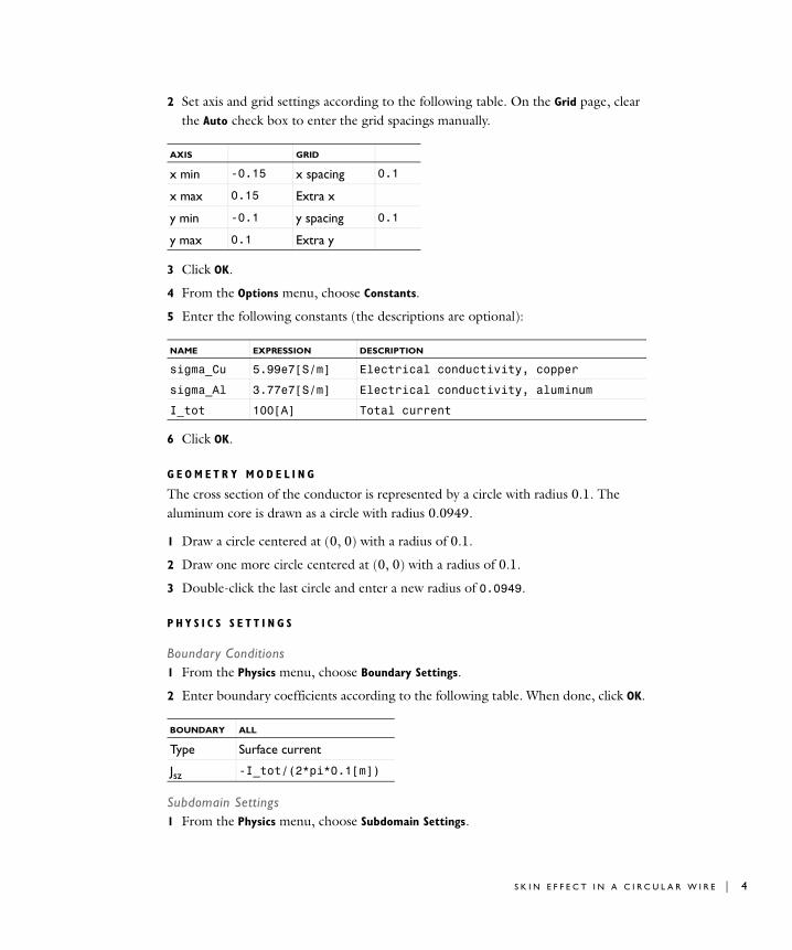
2 Set axis and grid settings according to the following table. On the Grid page, clear the Auto check box to enter the grid spacings manually.

3 Click OK.

4 From the Options menu, choose Constants.

5 Enter the following constants (the descriptions are optional):

6 Click OK.

G E O M E T R Y M O D E L I N G

The cross section of the conductor is represented by a circle with radius 0.1. The aluminum core is drawn as a circle with radius 0.0949.

1 Draw a circle centered at (0, 0) with a radius of 0.1.

2 Draw one more circle centered at (0, 0) with a radius of 0.1.

3 Double-click the last circle and enter a new radius of 0.0949.

P H Y S I C S S E T T I N G S

Boundary Conditions1 From the Physics menu, choose Boundary Settings.

2 Enter boundary coefficients according to the following table. When done, click OK.

Subdomain Settings1 From the Physics menu, choose Subdomain Settings.

AXIS GRID

x min -0.15 x spacing 0.1

x max 0.15 Extra x

y min -0.1 y spacing 0.1

y max 0.1 Extra y

NAME EXPRESSION DESCRIPTION

sigma_Cu 5.99e7[S/m] Electrical conductivity, copper

sigma_Al 3.77e7[S/m] Electrical conductivity, aluminum

I_tot 100[A] Total current

BOUNDARY ALL

Type Surface current

Jsz -I_tot/(2*pi*0.1[m])



2 Click the Electric Parameters tab.

3 Enter the subdomain settings (material property) according to the following table. When done, click OK.

M E S H G E N E R A T I O N

The small gap between the concentric circles gives you a fine mesh close to the boundaries, where the solution is expected to vary fastest. If you decrease the element growth rate, the mesh becomes smoother.

1 In the Free Mesh Parameters dialog box, click the Custom mesh size button and type 1.1 in the Element growth rate edit field. Click OK.

2 Initialize the mesh.

C O M P U T I N G T H E S O L U T I O N

Click the Solve button on the Main toolbar.

SETTING SUBDOMAINS 1, 2

σ sigma_Cu



PO S T P R O C E S S I N G A N D V I S U A L I Z A T I O N

Due to the skin effect, the current density at the surface is much higher than that within the interior of the conductor. Plotting the current density Jz clearly shows this effect.

1 Open the Plot Parameters dialog box.

2 Click the Surface tab.

3 On the Surface Data tab, select Total current density, z component from the Predefined

quantities list.

4 Click OK.

The resistance per meter is defined as R = P/I2, where P is the power loss per meter of wire, and I is the current through the power line. You can compute both the power and the current with integrations over the cross section:

where Q = σ|E|2. The value of the second integral is known a priori, because the total current is part of the boundary conditions.

1 From the Postprocessing menu, open the Subdomain Integration dialog box. Select both subdomains and choose the Total current density, z component from the Predefined quantities list. Click Apply and note that the total current is very close to 100 A, as expected.

2 Change the integration expression to Resistive heating, time average and click OK.

3 You can now compute the resistance per meter from R = P/I2.

Modeling a Wire with an Aluminum Core

Next, replace almost all copper with aluminum, leaving only a thin copper shell, and compare the results.

S U B D O M A I N S E T T I N G S

Change the conductivity in Subdomain 2 to sigma_Al.

C O M P U T I N G T H E S O L U T I O N

Solve the problem.

P Q Ad∫=

I Jz Ad∫=



PO S T P R O C E S S I N G

Now calculate the resistance per meter in the modified design.

1 From the Postprocessing menu, open the Subdomain Integration dialog box.

2 Select both subdomains and select Resistive heating, time average from the Predefined

quantities list.

3 Click OK.

4 Calculate the resistance per meter as before.

For a given current the combined copper/aluminum wire suffers approximately 10% more resistance compared to pure copper. On the other hand it weighs only one third and is considerably less expensive.


Documents

Skin Effect Sbs