Sketch-based 3D Shape Retrieval using Convolutional Neural Networks

Fang Wang1 Le Kang2 Yi Li1

1NICTA and ANU 2ECE, University of Maryland at College Park1{fang.wang, yi.li}@nicta.com.au, 2lekang@umiacs.umd.edu

Abstract

Retrieving 3D models from 2D human sketches has re-ceived considerable attention in the areas of graphics, im-age retrieval, and computer vision. Almost always in stateof the art approaches a large amount of “best views” arecomputed for 3D models, with the hope that the query sketchmatches one of these 2D projections of 3D models usingpredefined features.

We argue that this two stage approach (view selection– matching) is pragmatic but also problematic because the“best views” are subjective and ambiguous, which makesthe matching inputs obscure. This imprecise nature ofmatching further makes it challenging to choose featuresmanually. Instead of relying on the elusive concept of “bestviews” and the hand-crafted features, we propose to defineour views using a minimalism approach and learn featuresfor both sketches and views. Specifically, we drasticallyreduce the number of views to only two predefined direc-tions for the whole dataset. Then, we learn two SiameseConvolutional Neural Networks (CNNs), one for the viewsand one for the sketches. The loss function is defined onthe within-domain as well as the cross-domain similarities.Our experiments on three benchmark datasets demonstratethat our method is significantly better than state of the artapproaches, and outperforms them in all conventional met-rics.

1. IntroductionRetrieving 3D models from 2D sketches has impor-

tant applications in computer graphics, information re-trieval, and computer vision [9, 13, 18]. Compared to theearly attempts where keywords or 3D shapes are used asqueries [23], the sketch-based idea is very attractive becausesketches by hand provide an easy way to input, yet they arerich enough to specify shapes.

Directly matching 2D sketches to 3D models suffersfrom significant differences between the 2D and 3D repre-sentations. Thus, in many state of the art methods 3D mod-

Figure 1. Examples of sketch based 3D shape retrieval.

els are projected to multiple 2D views, and a sketch matchesa 3D model if it matches one of its views. Fig. 1 shows afew examples of 2D sketches and their corresponding 3Dmodels. One can immediately see the variations in both thesketch styles and 3D models.

In almost all state of the art approaches, sketch based3D shape retrieval amounts to finding the “best views” for3D models and hand-crafting the right features for match-ing sketches and views. First, an automatic procedure isused to select the most representative views of a 3D model.Ideally, one of the viewpoints is similar to that of the querysketches. Then, 3D models are projected to 2D planes usinga variety of line rendering algorithms. Subsequently, many2D matching methods can be used for computing the sim-ilarity scores, where features are always manually defined(e.g., Gabor, dense SIFT, and GALIF [9]).

This stage-wise methodology appears pragmatic, but italso brings a number of puzzling issues. To begin with,there is no guarantee that the best views have similar view-points with the sketches. The inherent issue is that identify-ing the best views is an unsolved problem on its own, par-tially because the general definition of best views is elusive.In fact, many best view methods require manually selectedviewpoints for training, which makes the view selection byfinding “best views” a chicken-egg problem.

Further, this viewpoint uncertainty makes it dubious tomatch samples from two different domains without learn-ing their metrics. Take Fig. 1 for example, even when the

viewpoints are similar the variations in sketches as well asthe different characteristics between sketches and views arebeyond the assumptions of many 2D matching methods.

Considering all the above issues arise when we strug-gle to seek the viewpoints for matching, can we bypass thestage of view selection? In this paper we demonstrate thatby learning cross domain similarities, we no longer requirethe seemingly indispensable view similarity assumption.

Instead of relying on the elusive concept of “best views”and hand-crafted features, we propose to define our viewsand learn features for views and sketches. Assuming thatthe majority of the models are upright, we drastically reducethe number of views to two per object for the whole dataset.We also make no selections of these two directions as longas they are significantly different. Therefore, we considerthis as the minimalism approach as opposed to multiple bestviews.

This upright assumption appears to be strong, but it turnsout to be sensible for 3D datasets. Many 3D models are nat-urally generated upright (e.g., [23]). We choose two view-points because it is very unlikely to get degenerated viewsfor two significantly different viewpoints. An immediateadvantage is that our matching is more efficient without theneed of comparing to more views than necessary.

This seemingly radical approach triumphs only when thefeatures are learned properly. In principle, this can be re-garded as learning representations between sketches andviews by specifying similarities, which gives us a seman-tic level matching. To achieve this, we need comprehensiveshape representations rather than the combination of shal-low features that only capture low level visual information.

We learn the shape representations using ConvolutionalNeural Network (CNN). Our model is based on the Siamesenetwork [5]. Since the two input sources have distinctiveintrinsic properties, we use two different CNN models, onefor handling the sketches and the other for the views. Thistwo model strategy can give us more power to capture dif-ferent properties in different domains.

Most importantly, we define a loss function to “align”the results of the two CNN models. This loss function cou-ples the two input sources into the same target space, whichallows us to compare the features directly using a simpledistance function.

Our experiments on three large datasets show that ourmethod significantly outperforms state of the art approachesin a number of metrics, including precision-recall and thenearest neighbor. We further demonstrate the retrievals ineach domain are effective. Since our network is based onfiltering, the computation is fast.

Our contributions include

• We propose to learn feature representations for sketchbased shape retrieval, which bypasses the dilemma ofbest view selection;

• We adopt two Siamese Convolutional Neural Net-works to successfully learn similarities in both thewithin-domain and the cross domain;

• We outperform all the state of the art methods on threelarge datasets significantly.

2. Related workSketch based shape retrieval has received many interests

for years [10]. In this section we review three key com-ponents in sketch based shape retrieval: public availabledatasets, features, and similarity learning.

Datasets The effort of building 3D datasets can be tracedback to decades ago. The Princeton Shape Benchmark(PSB) is probably one of the best known sources for 3Dmodels [23]. There are some recent advancements for gen-eral and special objects, such as the SHREC’14 Benchmark[20] and the Bonn Architecture Benchmark [27].

2D sketches have been adopted as input in many systems[6]. However, the large scale collections are available onlyrecently. Eitz et al. [9] collected sketches based on the PSBdataset. Li et al. [18] organized the sketches collected by[8] in their SBSR challenge.

Features Global shape descriptors, such as statistics ofshapes [21] and distance functions [15], have been used for3D shape retrieval [25]. Recently, local features is proposedfor partial matching [11] or used in the bag-of-words modelfor 3D shape retrieval [3].

Boundary information together with internal structuresare used for matching sketches against 2D projections.Therefore, a good representation of line drawing images isa key component for sketch based shape retrieval. Sketchrepresentation such as shape context [1] was proposed forimage based shape retrieval. Furuya et al. proposed BF-DSIFT feature, which is an extended SIFT feature withBag-of-word method, to represent sketch images [12]. Onerecent method is the Gabor local line based feature (GALIF)by Mathias et al., which builds on a bank of Gabor filtersfollowed by a Bag-of-word method [9].

In addition to 2D shape features, some methods also ex-plored geometry features as well as graph-based features tofacilitate the 3D shape retrieval [19]. Semantic labeling isalso used to bridge the gaps between different domains [14].In this paper, we focus on view based method and only use2D shape features.

CNN and Siamese network Recently deep learning hasachieved great success on many computer vision tasks.Specifically, CNN has set records on standard object recog-nition benchmarks [16]. With a deep structure, the CNN caneffectively learn complicated mappings from raw images to

the target, which requires less domain knowledge comparedto handcrafted features and shallow learning frameworks.

A Siamese network [5] is a particular neural network ar-chitecture consisting of two identical sub-convolutional net-works, which is used in a weakly supervised metric learn-ing setting. The goal of the network is to make the out-put vectors similar if input pairs are labeled as similar, anddissimilar for the input pairs that are labeled as dissimilar.Recently, the Siamese network has been applied to text clas-sification [28] and speech feature classification [4].

3. Learning feature representations for sketchbased 3D shape retrieval

We first briefly introduce basic concepts in CNNs andSiamese network. Then, we present our network architec-ture for cross domain matching, based on the Siamese net-work. Given a set of view and sketch pairs, we propose touse two different Siamese networks, one for each domain.Finally, we revisit the view selection problem, and describeour minimalism approach of viewpoint definition and theline drawing rendering procedure.

3.1. CNN and Siamese network

CNN is a multilayer learning framework, which consistsof an input layer, a few convolutional layers and fully con-nected layers, as well as an output layer on which the lossfunction is defined. The goal of CNN is to learn a hierarchyof feature representations. Signals in each layer are con-volved with a number of filters and further downsampledby pooling operations, which aggregate values in a smallregion by functions including max, min, and average. Thelearning of CNN is based on Stochastic Gradient Descent(SGD). Please refer to [17] for details.

Siamese Convolutional Neural Network has been usedsuccessfully for dimension reduction in weakly supervisedmetric learning. Instead of taking single sample as input, thenetwork typically takes a pair of samples, and the loss func-tions are usually defined over pairs. A typical loss functionof a pair has the following form:

L(s1, s2, y) = (1− y)αD2w + yβeγDw , (1)

where s1 and s2 are two samples, y is the binary similaritylabel,Dw = ‖f(s1;w1)− f(s2;w2)‖1 is the distance. Fol-lowing [5], we set α = 1

Cp, β = Cn, and γ = −2.77

Cn, where

Cp = 0.2 and Cn = 10 are two constants.This can be regarded as a metric learning approach. Un-

like methods that assign binary similarity labels to pairs, thenetwork aims at bring the output feature vectors closer forinput pairs that are labeled as similar, or push the featurevectors away if the input pairs are labeled as dissimilar.

The Siamese network is frequently illustrated as twoidentical networks for two different samples. In each SGD

iteration, pairs of samples are processed using two iden-tical networks, and the error computed by Eq. 1 is thenback-propagated and the gradients are computed individu-ally base on the two sample sets. The Siamese network isupdated by the average of these two gradients.

3.2. Cross-domain matching using Siamese network

In this section, we propose a method to match samplesfrom two domains without the heavy assumption of viewsimilarity. We first provide our motivation using an illus-trated sample. Then, we propose our extension of the basicSiamese network. Specifically, we use two different net-works to handle sources from different domains.

3.2.1 An illustrated example

The matching problem in sketch based shape retrieval canbe seen as a metric learning paradigm. In each domain,the samples are mapped to some feature vectors. The crossdomain matching is successful if the features from each do-main are “aligned” correctly.

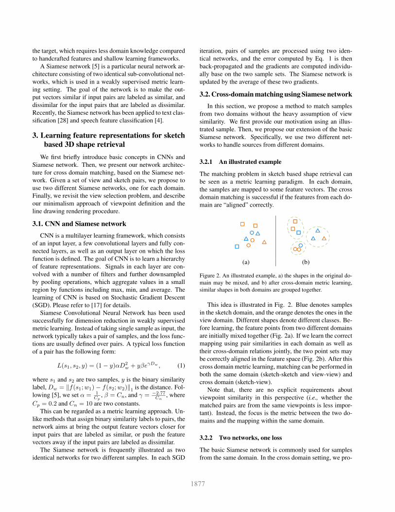
(a) (b)

Figure 2. An illustrated example, a) the shapes in the original do-main may be mixed, and b) after cross-domain metric learning,similar shapes in both domains are grouped together.

This idea is illustrated in Fig. 2. Blue denotes samplesin the sketch domain, and the orange denotes the ones in theview domain. Different shapes denote different classes. Be-fore learning, the feature points from two different domainsare initially mixed together (Fig. 2a). If we learn the correctmapping using pair similarities in each domain as well astheir cross-domain relations jointly, the two point sets maybe correctly aligned in the feature space (Fig. 2b). After thiscross domain metric learning, matching can be performed inboth the same domain (sketch-sketch and view-view) andcross domain (sketch-view).

Note that, there are no explicit requirements aboutviewpoint similarity in this perspective (i.e., whether thematched pairs are from the same viewpoints is less impor-tant). Instead, the focus is the metric between the two do-mains and the mapping within the same domain.

3.2.2 Two networks, one loss

The basic Siamese network is commonly used for samplesfrom the same domain. In the cross domain setting, we pro-

Figure 3. Dimension reduction using Siamese network.

pose to extend the basic version to two Siamese networks,one for the view domain and the other for the sketch do-main. Then, we define the within-domain loss and the crossdomain loss. This hypothesis is supported in the Sec. 4.

Assuming we have two inputs from each domain, i.e., s1and s2 are two sketches and v1 and v2 are two views. Forsimplicity, we assume s1 and v1 are from the same class ands2 and v2 are from the same class as well. Therefore, onelabel y is enough to specify their relationships.

As a result, our loss function is composed by three terms:the similarity of sketches, the similarity of views, and thecross domain similarity.

L(s1,s2, v1, v2, y)= L(s1, s2, y) + L(v1, v2, y) + L(s1, v1, y), (2)

where L(·, ·, ·) is defined by Eq. 1. Please note that, whilethe category information available in the dataset can be ex-ploited to improve the performance, we do not use the cate-gory labels in the above framework.

3.3. Network architecture

Fig. 3 shows the architecture of our network for the in-puts being views and sketches, respectively.

We use the same network design for both networks, butthey are learned separately. Our input patch size is 100×100for both sources. The structure of the single CNN has threeconvolutional layers, each with a max pooling, one fullyconnected layer to generate the features, and one outputlayer to compute the loss (Eq. 2).

The first convolutional layer followed by a 4× 4 poolinggenerates 32 response maps, each of size 22× 22. The sec-ond layer and pooling outputs 64 maps of size 8 × 8. Thethird layer layer has 256 response maps, each pooled to asize of 3×3. The 2304 features generated by the final pool-

ing operation are linearly transformed to 64× 1 features inthe last layer. Rectified linear units are used in all layers.

3.4. View definitions and line drawing rendering

We present our procedure of generating viewpoints andrendering 3D models. As opposed to multiple views, wefind it sufficient to use two views to characterize a 3D modelbecause the chance that both views are degenerated is little.Following this observation, we impose the minimal assump-tions on choosing views for the whole dataset:

1. Most of the 3D models in the dataset are up-right;

2. Two viewpoints are randomly generated for the wholedataset, provided that the difference in their angles islarger than 45 degrees.

Fig. 4 shows some of our views in the PSB dataset. Thefirst row shows that the upright assumption does not requirestrict alignments of 3D models, because some models maynot have well defined orientation. Further, while the modelsare upright, they can still has different rotations.

Figure 4. 3D models viewed from predefined viewpoints.

We want to stress that our approach does not eliminatethe possibility of selecting more (best) views as input, butthe comparisons among view selection methods are beyondthe scope of this paper.

Once the viewpoints are chosen, we render the 3D mod-els and generate 2D line drawings. Rendering line draw-ings that include strong abstraction and stylization effects isa very useful topic in computer graphics, computer vision,and psychology. Outer edges and internal edges both playan important role in this rendering process. Therefore, weuse the following descriptors: 1) closed boundaries and 2)Suggestive Contours [7] (Fig. 5).

(a) Shaded (b) SC (c) Final

Figure 5. Rendering 3D models.

4. ExperimentsWe present our experiments on three recent large datasets

in this section. In all experiments our method outperformsthe state of the arts in a number of well recognized metrics.In additional to the cross-domain retrieval, we also presentour within-domain retrieval results, which have not beenreported in any other comparison methods. These experi-ments demonstrate that our Siamese network successfullylearns the feature representations for both domains. Thedata and the code is available at http://users.cecs.anu.edu.au/˜yili/cnnsbsr/.

4.1. Datasets

PSB / SBSR dataset The Princeton Shape Benchmark(PSB) [23] is widely used for 3D shape retrieval systemevaluation, which contains 1814 3D models and is equallydivided into training set and testing set.

In [9], the Shape Based Shape Retrieval (SBSR) datasetis collected based on the PSB dataset. The 1814 handdrawn sketches are collected using Amazon MechanicalTurk. In the collection process, participants are asked todraw sketches given only the name of the categories with-out any visual clue from the 3D models.

SHREC’13 & ’14 dataset Although the PSB dataset iswidely used in shape retrieval evaluation, there is a con-cern that the number of sketches for each class in the SBSRdataset is not enough. Some classes have only very fewinstances (27 of 90 training classes have no more than 5instances), while some classes have dominating number ofinstances, e.g., the “fighter jet” class and the “human” classhave as many as 50 instances.

To remove the possible bias when evaluating the re-trieval algorithms, Li et al. [18] reorganized the PSB/SBSRdataset, and proposed a SHREC’13 dataset where a subset

of PSB with 1258 models is used and the sketches in eachclasses has 80 instances. These sketch instances are split intwo sets: 50 for training and 30 for testing. Please note, thenumber of models in each class still varies. For example,the largest class has 184 instances but there are 23 classescontaining no more than 5 models

Recently, SHREC’14 is proposed to address some aboveconcerns [20], which greatly enlarges the number of 3Dmodels to 8987, and the number of classes is doubled. Thelarge variation of this dataset makes it much more challeng-ing, and the overall performance of all reported methods arevery low (e.g., the accuracy for the best algorithm is only0.16 for the top 1 candidate). This is probably due to thefact that the models are from various sources and are arbi-trarily oriented. While our performance is still superior (seeFig. 9b and Table. 3), we choose to present our results usingthe SHREC’13 dataset.

Evaluation criteria In our experiment, we use the abovedatasets and measure the performance using the followingcriteria: 1) Precision-recall curve is calculated for eachquery and linear interpolated, then the final curve is reportedby averaging all precision values for fixed recall rates; 2)Average precision (mAP) is the area under the precision-recall curve; 3) Nearest neighbor (NN) is used to measurethe top 1 retrieval accuracy; 4) E-Measure (E) is the har-monic mean of the precision and recall for the top 32 re-trieval results; 5) First/second tier (FT/ST) and Discountedcumulated gain (DCG) as defined in the PSB statistics.

4.2. Experimental settings

Stopping criteria All three of the datasets had been splitinto training and testing sets, but no validation set wasspecified. Therefore, we terminated our algorithm after 50epochs for PSB/SBSR and 20 for SHREC’13 dataset (oruntil convergence). Multiple runs were performed and themean values were reported.

Generating pairs for Siamese network To make surewe generate reasonable proportion of similar and dissimilarpairs, we use the following approach to generate pair sets.For each training sketch, we random select kp view pairsin the same category (matched pairs) and kn view samplesfrom other categories (unmatched pairs). Usually, our dis-similar pairs are ten times more than the similar pairs forsuccessful training. In our experiment, we use kp = 2,kn = 20. We perform this random pairing for each train-ing epoch. To increase the number of training samples, wealso used data augmentation for the sketch set. To be spe-cific, we randomly perform affine transformations on eachsketch sample with small scales and angles to generate morevariations. We generate two augmentations for each sketchsample in the dataset.

Figure 6. Retrieval examples of PSB/SBSR dataset. Cyan denotes the correct retrievals.

Computational cost The implementation of the proposedSiamese CNN is based on the Theano [2] library. We mea-sure the processing time on on a PC with 2.8GHz CPU andGTX 780 GPU. With preprocessed view features, the re-trieval time for each query is approximately 0.002 sec onaverage on SHREC’13 dataset.

The training time is proportional to the total num-ber of pairs and the number of epochs. Overall trainingtakes approximately 2.5 hours for PSB/SBSR, 6 hours forSHREC’13, respectively. Considering the total number ofpairs is large, the training time is sensible.

We test various number of views in our experiments. Wefind that there was no significant performance gain whenwe vary the view from two to ten. However, it increased thecomputational cost significantly when more views are used,and more importantly, the GPU memory. This motivates usto select only two views in the experiments.

4.3. Shape retrieval on PSB/SBSR dataset

4.3.1 Examples

In this section, we test our method using the PSB/SBSRdataset. First, we show some retrieval examples in Fig. 6.The first column shows 8 queries from different classes, andeach row shows the top 15 retrieval results. Cyan denotesthe correct retrievals, and gray denotes incorrect ones.

Our method performs exceptionally well in popularclasses such as human, face, and plane. We also find thatsome fine grained categorizations are difficult to distin-guish. For instance, the shelf and the box differ only in asmall part of the model. However, we also want to notethat some of the classes only differ in semantics (e.g., barn

and house only differ in function). Certainly, this semanticambiguity is beyond the scope of this paper.

Finally, we want to stress that the importance of view-point is significantly decreased in our metric learning ap-proach. Some classes may exhibit a high degree of freedomsuch as the plane, but the retrieval results are also excellent(as shown in Fig. 6).

4.3.2 Analysis

We further show some statistics on this dataset. First, weprovide the precision-recall values at fixed points in Table1. Compared to Fig. 9 in [9], our results are approximately10% higher. We then show six standard evaluation metricsin Table 2. Since other methods did not report the resultson this dataset, we leave the comprehensive comparison tothe next section. Instead, in this analysis we focus on theeffectiveness of metric learning for shape retrieval.

PSB/SBSR is a very imbalanced dataset, where train-ing and testing only partially overlap. Namely, there are21 classes appear in both training and testing sets, while 71classes are used solely for testing. This makes it an excel-lent dataset for investigating similarity learning, because the“unseen” classes verify the learning is not biased.

We show some examples for these unseen classes in Fig.7 (more statistical curves are available on project websitedue to the space limitation). It is interesting to see that ourproposed method works well even on failure cases (e.g., theflower), where the retrieval returns similar shapes (“pottingplant”). This demonstrates that our method learns the simi-larity effectively.

Table 1. Precision-recall on fixed points.5% 20% 40% 60% 80% 100%

0.616 0.286 0.221 0.180 0.138 0.072

Table 2. Standard metrics on the PSB/SBSR dataset.NN FT ST E DCG mAP

0.223 0.177 0.271 0.173 0.451 0.218

Figure 7. Retrieval examples of unseen samples in PSB/SBSRdataset. The cyan denotes the correct retrievals.

4.4. Shape retrieval on SHREC’13 dataset

In this section, we use the SHREC’13 benchmark toevaluate our method. We also show the retrieval resultswithin the same domain.

4.4.1 A visualization of the learned features

First, we present a visualization of our learned features inFig. 8. We perform PCA on the learned features and re-duce the dimension to two for visualization. The greendots denote the sketches, and the yellow ones denote views.For simplicity, we only overlay the views over the pointcloud. Please visit http://users.cecs.anu.edu.au/˜yili/cnnsbsr/ for an interactive demo.

While this is a coarse visualization, we can already seesome interesting properties of our method. First, we can seethat classes with similar shapes are grouped together auto-matically. On the top right, different animals are mapped toneighboring positions. On the left, various types of vehiclesare grouped autonomously. Other examples include houseand church, which are very similar. Note that this is anweakly supervised method. This localization suggests thatthe learned features are very useful for both within-domainand cross domain retrievals.

4.4.2 Statistical results

We present the statistical results on SHREC’13 in this sec-tion. First, we compare the precision-recall curve againstthe state of the art methods reported in [18].

From the Fig. 9 we can see that our method significantlyoutperforms other comparison methods. On SHREC’13

Figure 8. Visualization of feature space on SHREC’13. Sketch andview feature points are shown by green & yellow, respectively.

benchmark, the performance gain of our method is already10% when recall is small. More importantly, the wholecurve decreases much slower than other methods when therecall increases, which is desirable because it shows themethod is more stable. Our method has a higher perfor-mance gain (30%) when recall reaches 1.

We note that there is a noticeable overfitting in the train-ing when a stopping criterion is reached. It suggests theperformance can be even better, if one can fine tune andexplore the network structure and training procedure.

We further show the standard metrics for comparison.These metrics examine the retrieval from different perspec-tives. For simplicity, we only select the best method fromeach research group in [18]. As shown in Table 3, ourmethod performs better in every metric on both bench-marks. This further demonstrates our method is superior.

We also compare to the case where both networksare identical, i.e., both views and sketches use the sameSiamese network. Fig. 9a suggests that this configura-tion is inferior than our proposed version, but still it is bet-ter than all other methods. This supports our hypothesisthat the variations in two domains are different. This alsosends a message that using the same features (hand-craftedor learned) for both domains may not be ideal.

4.4.3 Within-domain retrieval

Finally, we show the retrievals in the same domain. Thisinteresting experiment shall be straightforward to report be-cause the data is readily available, but was not shown before

0 0.2 0.4 0.6 0.8 10

0.1

0.2

0.3

0.4

0.5

0.6

Recall

Pre

cis

ion

Ours Siamese Model

Ours Identic Model

Furuya (CDMR−BF−fGALIF+CDMR−BF−fDSIFT)

Furuya (CDMR−BF−fGALIF)

Furuya (BF−fGALIF+BF−fDSIFT)

Furuya (UMR−BF−fGALIF+UMR−BF−fDSIFT)

Furuya (CDMR−BF−fDSIFT)

Furuya (BF−fGALIF)

Furuya (UMR−BF−fDSIFT)

Li (SBR VC−NUM−100)

Furuya (UMR−BF−fGALIF)

Furuya (BF−fDSIFT)

Li (SBR 2D−3D−NUM−50)

Saavedra (HOG−SIL)

Li (SBR VC−NUM−50)

Saavedra (HELO−SIL)

Saavedra (FDC−CVIU version)

Saavedra (FDC)

Pascoal (HTD)

Aono (EFSD)

0 0.2 0.4 0.6 0.8 10

0.1

0.2

0.3

0.4

0.5

0.6

Recall

Pre

cis

ion

Ours

Tatsuma (SCMR−OPHOG)

Tatsuma (OPHOG)

Furuya (CDMR (sigma_SM=0.05, alpha=0.3))

Furuya (CDMR (sigma_SM=0.1, alpha=0.3))

Furuya (BF−fGALIF)

Li (SBR−VC (alpha=1))

Furuya (CDMR (sigma_SM=0.05, alpha=0.6))

Li (SBR−VC (alpha=0.5))

Furuya (CDMR (sigma_SM=0.1, alpha=0.6))

Zou (BOF−JESC (Words800_VQ))

Zou (BOF−JESC (FV_PCA32_Words128))

Zou (BOF−JESC (Words1000_VQ))

(a) SHREC’13 comparison (b) SHREC’14 comparison

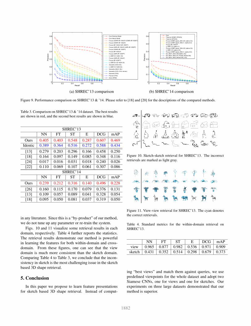
Figure 9. Performance comparison on SHREC’13 & ’14. Please refer to [18] and [20] for the descriptions of the compared methods.

Table 3. Comparison on SHREC’13 & ’14 dataset. The best resultsare shown in red, and the second best results are shown in blue.

SHREC’13NN FT ST E DCG mAP

Ours 0.405 0.403 0.548 0.287 0.607 0.469Identic 0.389 0.364 0.516 0.272 0.588 0.434

[13] 0.279 0.203 0.296 0.166 0.458 0.250[18] 0.164 0.097 0.149 0.085 0.348 0.116[24] 0.017 0.016 0.031 0.018 0.240 0.026[22] 0.110 0.069 0.107 0.061 0.307 0.086

SHREC’14NN FT ST E DCG mAP

Ours 0.239 0.212 0.316 0.140 0.496 0.228[26] 0.160 0.115 0.170 0.079 0.376 0.131[13] 0.109 0.057 0.089 0.041 0.328 0.054[18] 0.095 0.050 0.081 0.037 0.319 0.050

in any literature. Since this is a “by-product” of our method,we do not tune up any parameter or re-train the system.

Figs. 10 and 11 visualize some retrieval results in eachdomain, respectively. Table 4 further reports the statistics.The retrieval results demonstrate our method is powerfulin learning the features for both within-domain and cross-domain. From these figures, one can see that the viewdomain is much more consistent than the sketch domain.Comparing Table 4 to Table 3, we conclude that the incon-sistency in sketch is the most challenging issue in the sketchbased 3D shape retrieval.

5. Conclusion

In this paper we propose to learn feature presentationsfor sketch based 3D shape retrieval. Instead of comput-

Figure 10. Sketch-sketch retrieval for SHREC’13. The incorrectretrievals are marked as light gray.

Figure 11. View-view retrieval for SHREC’13. The cyan denotesthe correct retrievals.

Table 4. Standard metrics for the within-domain retrieval onSHREC’13.

NN FT ST E DCG mAPview 0.965 0.877 0.982 0.536 0.971 0.909

sketch 0.431 0.352 0.514 0.298 0.679 0.373

ing “best views” and match them against queries, we usepredefined viewpoints for the whole dataset and adopt twoSiamese CNNs, one for views and one for sketches. Ourexperiments on three large datasets demonstrated that ourmethod is superior.

6. AcknowledgementNICTA is funded by the Australian Government as rep-

resented by the Department of Broadband, Communica-tions and the Digital Economy and the Australian ResearchCouncil through the ICT Centre of Excellence program.

References[1] S. Belongie, J. Malik, and J. Puzicha. Shape matching and

object recognition using shape contexts. IEEE Trans. PatternAnal. Mach. Intell., 24(4):509–522, Apr. 2002.

[2] J. Bergstra, O. Breuleux, F. Bastien, P. Lamblin, R. Pascanu,G. Desjardins, J. Turian, D. Warde-Farley, and Y. Bengio.Theano: a CPU and GPU math expression compiler. In Pro-ceedings of the Python for Scientific Computing Conference(SciPy), Jun. 2010.

[3] A. M. Bronstein, M. M. Bronstein, L. J. Guibas, and M. Ovs-janikov. Shape google: Geometric words and expressionsfor invariant shape retrieval. ACM Trans. Graph., 30(1):1:1–1:20, Feb. 2011.

[4] K. Chen and A. Salman. Extracting speaker-specific in-formation with a regularized siamese deep network. InJ. Shawe-Taylor, R. Zemel, P. Bartlett, F. Pereira, andK. Weinberger, editors, NIPS 2011, pages 298–306. 2011.

[5] S. Chopra, R. Hadsell, and Y. LeCun. Learning a similaritymetric discriminatively, with application to face verification.In CVPR 2005, volume 1, pages 539–546. IEEE, 2005.

[6] P. Daras and A. Axenopoulos. A 3d shape retrieval frame-work supporting multimodal queries. International Journalof Computer Vision, 89(2-3):229–247, 2010.

[7] D. DeCarlo, A. Finkelstein, S. Rusinkiewicz, and A. San-tella. Suggestive contours for conveying shape. ACM Transon Graphics, 22(3):848–855, July 2003.

[8] M. Eitz, J. Hays, and M. Alexa. How do humans sketchobjects? ACM Trans. on Graphics, 31(4):44:1–44:10, 2012.

[9] M. Eitz, R. Richter, T. Boubekeur, K. Hildebrand, andM. Alexa. Sketch-based shape retrieval. ACM Trans. Graph-ics, 31(4):31:1–31:10, 2012.

[10] T. Funkhouser, P. Min, M. Kazhdan, J. Chen, A. Halderman,D. Dobkin, and D. Jacobs. A search engine for 3D models.ACM Transactions on Graphics, 22(1):83–105, Jan. 2003.

[11] T. Funkhouser and P. Shilane. Partial matching of 3d shapeswith priority-driven search. In Proceedings of the Fourth Eu-rographics Symposium on Geometry Processing, pages 131–142. Eurographics Association, 2006.

[12] T. Furuya and R. Ohbuchi. Dense sampling and fast encod-ing for 3d model retrieval using bag-of-visual features. InProceedings of the ACM international conference on imageand video retrieval, page 26. ACM, 2009.

[13] T. Furuya and R. Ohbuchi. Ranking on cross-domain man-ifold for sketch-based 3d model retrieval. In InternationalConference on Cyberworlds 2013, pages 274–281. IEEE,2013.

[14] B. Gong, J. Liu, X. Wang, and X. Tang. Learning semanticsignatures for 3d object retrieval. Multimedia, IEEE Trans-actions on, 15(2):369–377, 2013.

[15] M. M. Kazhdan, B. Chazelle, D. P. Dobkin, A. Finkel-stein, and T. A. Funkhouser. A reflective symmetry descrip-tor. ECCV ’02, pages 642–656, London, UK, UK, 2002.Springer-Verlag.

[16] A. Krizhevsky, I. Sutskever, and G. Hinton. Imagenet clas-sification with deep convolutional neural networks. In NIPS,2012.

[17] Y. LeCun and Y. Bengio. The handbook of brain theory andneural networks. chapter Convolutional networks for images,speech, and time series, pages 255–258. MIT Press, Cam-bridge, MA, USA, 1998.

[18] B. Li, Y. Lu, A. Godil, T. Schreck, B. Bustos, A. Ferreira,T. Furuya, M. J. Fonseca, H. Johan, T. Matsuda, et al. A com-parison of methods for sketch-based 3d shape retrieval. Com-puter Vision and Image Understanding, 119:57–80, 2014.

[19] B. Li, Y. Lu, C. Li, A. Godil, T. Schreck, M. Aono,M. Burtscher, Q. Chen, N. K. Chowdhury, B. Fang, et al. Acomparison of 3d shape retrieval methods based on a large-scale benchmark supporting multimodal queries. ComputerVision and Image Understanding, 131:1–27, 2015.

[20] B. Li, Y. Lu, C. Li, A. Godil, T. Schreck, M. Aono, Q. Chen,N. Chowdhury, B. Fang, T. Furuya, H. Johan, R. Kosaka,H. Koyanagi, R. Ohbuchi, and A. Tatsuma. SHREC14 track:Comprehensive 3d shape retrieval. In Proc. EG Workshop on3D Object Retrieval, 2014.

[21] R. Osada, T. Funkhouser, B. Chazelle, and D. Dobkin. Shapedistributions. ACM Transactions on Graphics, 21(4):807–832, Oct. 2002.

[22] J. M. Saavedra, B. Bustos, T. Schreck, S. Yoon, andM. Scherer. Sketch-based 3d model retrieval using keyshapesfor global and local representation. In EG 3DOR’12, pages47–50. Eurographics Association, 2012.

[23] P. Shilane, P. Min, M. Kazhdan, and T. Funkhouser. Theprinceton shape benchmark. In Shape modeling applications,2004. Proceedings, pages 167–178. IEEE, 2004.

[24] P. M. A. Sousa and M. J. Fonseca. Sketch-based retrievalof drawings using spatial proximity. J. Vis. Lang. Comput.,21(2):69–80, 2010.

[25] J. W. Tangelder and R. C. Veltkamp. A survey of contentbased 3d shape retrieval methods. Multimedia Tools Appl.,39(3):441–471, Sept. 2008.

[26] A. Tatsuma, H. Koyanagi, and M. Aono. A large-scale shapebenchmark for 3d object retrieval: Toyohashi shape bench-mark. Signal and Information Processing Association, pages3–6, 2012.

[27] R. Wessel, I. Blumel, and R. Klein. A 3d shape bench-mark for retrieval and automatic classification of architec-tural data. In 3DOR ’09, pages 53–56. Eurographics Associ-ation, 2009.

[28] W. Yih, K. Toutanova, J. C. Platt, and C. Meek. Learningdiscriminative projections for text similarity measures. InProceedings of the Fifteenth Conference on ComputationalNatural Language Learning, CoNLL ’11, pages 247–256,2011.