1

Sizing Linear and PWM Amplifiers Driving aLinear Brushless Motor

Varedan Technologies Technical Staff †

Abstract—This application note provides a design process forsizing linear and PWM three-phase amplifiers driving a linearbrushless motor (LBM). Design inputs consist of the motorforce constant, back-emf constant, pitch, winding resistanceand inductance, the load mass, and the worst-case velocity andload force profiles. The design outputs are the five key amplifierrequirements: amplifier bus voltage(s), peak output current,continuous output current, peak output power, and continuouspower dissipation. The design outputs peak output power andcontinuous power dissipation only apply to the sizing of linearamplifiers. Special attention is given to trapezoidal velocityprofiles and piecewise-constant load force profiles, which areused in a companion spreadsheet [1]. Equations for powersupply sizing and motor heating power are also provided.

Index Terms—Amplifier Sizing, PWM Amplifier, LinearAmplifier, Linear Brushless Motor, Varedan Document 4083-42-005 Revision C

I. INTRODUCTION

This document provides background and design equationsfor sizing linear and pulse-width modulated (PWM) ampli-fiers driving a three-phase linear brushless motor (LBM).The companion design spreadsheet [1] incorporates thedesign equations of Section IV below and provides an easy-to-use tool that will meet the needs of most designers. Theanalyses contained here can provide valuable context andhelp the designer understand limits of the design spreadsheet.

It is useful to think of amplifier sizing as a design processthat incorporates design inputs and design outputs. For anLBM system design, the following design inputs are usedto size an amplifier. SI units are used throughout unlessotherwise noted.• Motor force constant Kf (N/Arms)• Motor phase-to-phase back-emf constant Ke

((Vφφ peak)/(m/sec))• Motor phase-to-phase resistance Rφφ (Ω)• Motor phase-to-phase inductance Lφφ (H)• Motor pitch p (m)• Motor load mass m (kg)• Worst-case velocity profile v(t) (m/sec)• Worst-case load force profile Fload(t) (N)

The design methodology described herein produces designoutputs that consist of five key amplifier requirements below.Peak output power and continuous power dissipation are

†Copyright c© 2017 Varedan Technologies, 3860 Del Amo Blvd #401,Torrance, CA 90503, phone: (310) 542-2320, website: www.varedan.com,email: sales@varedan.com

design outputs that apply only to linear amplifier sizing asthe specifications for output current in PWM amplifiers aresufficient to determine power dissipation – these are markedwith an asterisk (*). The amplifier selection requirementsare:

• Bipolar Amplifier Bus Voltage ±B for linear amplifiers(Amplifier Bus Voltage 2B for PWM amplifiers)

• Peak Output Current Ipeak• Continuous Output Current Icont• Peak Output Power* Ppeak• Continuous Power Dissipation* PcontOnce the amplifier requirements are determined, a linear

or PWM amplifier is sized with specifications that meet orexceed the requirements.

The remainder of this application note is organized asfollows: In Section II, the design inputs are discussed andclearly defined. Algebraic equations that relate the designinputs to the design outputs are presented in Section III,and these equations are specialized to a trapezoidal velocityprofile and a piecewise-constant load force profile in SectionIV. The equations for a trapezoidal profile are implementedin the spreadsheet [1]. Section V contains some simpledesign checks. A numerical sizing example is given inSection VI, and some auxiliary equations for power supplysizing and motor ohmic heating are provided in Section VII.Section VIII makes some conclusions.

Fig. 1. Schematic diagram of a three-phase moving-magnet linear brushlessmotor.

2

II. BACKGROUND & DESIGN INPUTS

The notation describing a three-phase LBM is introducedin this section together with definitions of the design in-puts used for amplifier sizing. Consider first the simplifiedschematic of a moving magnet LBM depicted in Fig. 1,which helps visualize the phase-to-phase voltages, the phasecurrents, and the load velocity. Moreover, two of manyperiods of the magnet array are shown, and the spatial periodof the magnet array, referred to as the pitch p, is indicated.The spacing between the phase windings is p/3 and thuscreates the symmetric electrical properties common to allthree-phase LBMs.

Currents in phases A, B, and C produce forces on themoving magnets, and the motion of the magnets induceback-emf voltages in the phases. The motor force and back-emf constants are defined in terms of the motor currents,voltages, force, and velocity as follows.

A. Motor force constant Kf (N/Arms)

There are various definitions of motor force constantwhich capture, in rough terms, the ratio (amount of motorforce)÷ (amount of motor current). Up to a choice of units,the “amount of motor force” is clear. However, there arevarious ways to measure the currents in an LBM. There arethree sinusoidal phase currents and each current can be mea-sured with an root-mean-square (rms) current measurementor a peak current measurement. A common measurement ofcurrent in the three phases is the rms current in a singlephase where it is understood that the phases are drivenwith a sinusoidal current of that same magnitude and havingphases separated by 120. To indicate this convention, thecurrent unit in the force-constant is labeled with rms as inN/Arms (that all phases are driven is implied).

To be clear, consider the typical sinusoidal phase-currentwaveforms IA, IB , and IC applied to an LBM are depictedin Figure 2.

Fig. 2. Three-phase symmetrical current set used to drive an LBM. Thefigure depicts Irms, which is used in the definition of Kf .

The current waveforms have an obvious symmetry andare referred to as a three-phase symmetrical current set.The three sinusoidal currents collectively produce a constantforce F , and their frequency is determined by the motorvelocity v and the commutation process. The rms currentfor each phase is the same and denoted by Irms. The motorforce constant with an rms current measurement is definedby

Kf ≡ F/Irms, (1)

where the symbol ≡ is read “defined equal to.” The forceconstant units are “force per amp rms” which is abbreviatedforce/Arms. In the following sections, the SI force unitnewton is used and Kf is expressed in N/Arms.

Since the peak current is√

2 times the rms current, aforce constant expressed as force/Apeak can be convertedto force/Arms by multiplying the first number by

√2 as

summarized in Table I. The rms unit is used in the nextsections and in the companion spreadsheet [1]. Again, ineither unit definition, it is assumed that the three phases aredriven with a symmetrical current set.

When computing the motor force F for evaluation inEquation 1, both inertial and load force terms are included.Let a(t) ≡ dv

dt denote the acceleration and then one obtains

F = ma(t) + Fload. (2)

The mass include mass reflected through any linkage orgearbox mechanism as described below.

B. Motor phase-to-phase back-emf constant Ke

(Vφφ peak/(rad/s))

An LBM acts as a generator, and when the magnet arrayis moved relative to the stationary phase windings voltagesare produced across the phase windings. That is, the motorcreates an electromotive force (emf), which is consideredbackward by common sign conventions and is thus calledthe back emf. If the “generator” phase terminals are discon-nected or otherwise unloaded, the sinusoidal phase-to-phasevoltages have the same amplitude and frequency.

In the sections below, the back emf voltage is measuredphase-to-phase and its peak value is used. The units aresubscripted with φφ to indicate “phase-to-phase” and withpeak to indicate that the peak value of voltage is used. Figure3 shows Vφφ peak graphically. SI units are used herein so thatvelocity is expressed in m/sec.

Note that the frequency of the phase-to-phase voltagesinusoids, as are their amplitudes, are proportional to themotor velocity.

Unit Multiply By To Get

force/Apeak√2 force/Arms

TABLE IFORCE CONSTANT CONVERSION FACTOR

3

Fig. 3. Phase-to-phase voltage waveforms used in defining the back-emfconstant Ke.

Since the back-emf voltage is proportional to velocity, andin reference to Figure 3, the back emf constant Ke is definedby

Ke ≡ Vφφ peak/v. (3)

The same Ke would be calculated at the higher velocity v′

in Figure 3 with the proportionally higher peak voltage.

Fig. 4. Four ways to measure the back-emf voltage (Vφφ peak , Vφφ rms,Vφn peak , Vφn rms). Vφφ peak is the measure used in this application noteand in the spreadsheet [1].

Unfortunately, there are four natural definitions for theback-emf constant that quantify the ratio (amount of back-emf voltage)÷ (motor speed). The definition based on phase-to-phase peak voltage is the one used in this application noteand in [1], and there are three other definitions. In definingthe back-emf voltage, there is a choice of where to measurea voltage (phase-to-phase or phase-to-neutral) and a choicebetween rms voltage or peak voltage. Thus, there are fournatural measurements not to mention various units used forvelocity (see Figure 4) and the design engineer must be clearon which measurement is used.

In reference to Figure 4, the peak voltage of a sinusoid is√2 times the rms voltage, and the amplitude of the phase-

to-phase back-emf voltage Vφφ is√

3 times the amplitudeof the phase-to-neutral back-emf voltage Vφn. These ratioslead to the unit conversions of Table II where the speed unitis arbitrary, but constant, throughout the table.

C. Phase-to-phase resistance Rφφ (Ω) and inductance Lφφ(H)

Figure 1 shows the individual phase windings as havingresistance Rφφ/2 and inductance Lφφ/2 such that the resis-tance and inductance measured across two phase terminalsare Rφφ and Lφφ respectively.

D. Motor pitch p (m)

The motor pitch p is the spatial period of the magnet arrayin the motor. It is the distance between the north poles or,equivalently, the distance between the south poles.

E. Mass m (kg)

The mass m is the total moving mass internal and externalto the motor. The internal mass is usually listed in the motordata sheet and the external mass includes mass reflectedthrough any linkage or gearbox mechanism. As usual, anymass on the output of a linkage or gearbox is multiplied bythe square of the speed ratio (output speed/input speed).

F. Worst-case velocity and load force profilesA necessary design input for selecting an amplifier is one

or more worst-case velocity profiles and load force profiles.The accelerations, loads, peak velocities, and other featuresof these profiles inform the amplifier selection. In choosingworst-case profiles, it is useful to understand how they affectthe various design outputs. Further, such understanding canguide the system design and engineers may alter motiontrajectories to reduce amplifier cost. A qualitative discussionof the velocity and load force profiles’ impact on each ofthe design outputs is contained in subsections 1-5 below.

1) Peak Output Current: Short-time-constant thermallimits in connectors constrain the amplifier peak output cur-rent. Since large currents are needed to produce high forces,velocity profiles with high peak accelerations and load forceswill place demanding requirements on the peak output cur-rent. Even a generally low-velocity low-acceleration profilecan be challenging in terms of peak output current if thereare short bursts of high inertial or load forces.

Unit Multiply By To Get

Vφφ rms/speed√2 Vφφ peak/speed

Vφn peak/speed√3 Vφφ peak/speed

Vφn rms/speed√6 Vφφ peak/speed

TABLE IIBACK-EMF CONSTANT CONVERSION FACTORS

4

2) Continuous Output Current: Long time constants as-sociated with conductor heating constrain the continuousoutput current. Trajectories that repeatedly accelerate anddecelerate the load mass, or require high load forces, cancause overheating of conductors by exceeding the highcontinuous output current specification of an amplifier.

3) Peak Output Power*: As indicated by the asterisk, thepeak output power calculated herein is used in sizing linearamplifiers only. In a linear amplifier, the peak output poweris that peak power experienced by a single output transistor,or set of paralleled output transistors when acting as a singledevice. Heavy braking at high speeds causes large voltagedrops and high currents in the output transistors, leading tohigh power dissipation. The peak output power dissipatedin the transistors of a PWM amplifier is determined by thepeak output current and a separate constraint on peak outputpower is redundant. High load forces with large outputtransistor voltage drops also cause high power dissipationin the output transistors.

4) Continuous Power Dissipation*: As indicated by theasterisk, the continuous power dissipation calculated hereinapplies to linear amplifiers only. Trajectories that repeatedlyimpose high inertial or load forces cause high continu-ous power dissipation in the output transistors of linearamplifiers. Over time, the temperature of the heat sinkrises and the junction temperature of the power transistorscan exceed specifications. The continuous power dissipationin the transistors of a PWM amplifier is determined bythe continuous output current and a separate constraint oncontinuous power dissipation is redundant.

5) Bipolar Amplifier Bus Voltage for linear amplifiers,Amplifier Bus Voltage for PWM amplifiers: The bus-to-bus voltage in a linear or PWM amplifier must exceedthe largest back-emf voltages, which are sinusoidal withzero mean. Thus, high-speed trajectories and/or motors withlarge back-emf constants can exceed the capabilities of thepower supply/amplifier system. In linear amplifiers, the busvoltages are +B Volts and −B Volts and are referred to asthe “bipolar amplifier bus voltage ±B.” In PWM amplifiers,the bus voltages are 0Volts and 2B Volts where the latteris normally referred to as the bus voltage and the bus at0Volts is implied. The variable B is used in specifying bothamplifier types in order to simplify notation. In either case,the bus-to-bus voltage is 2B.

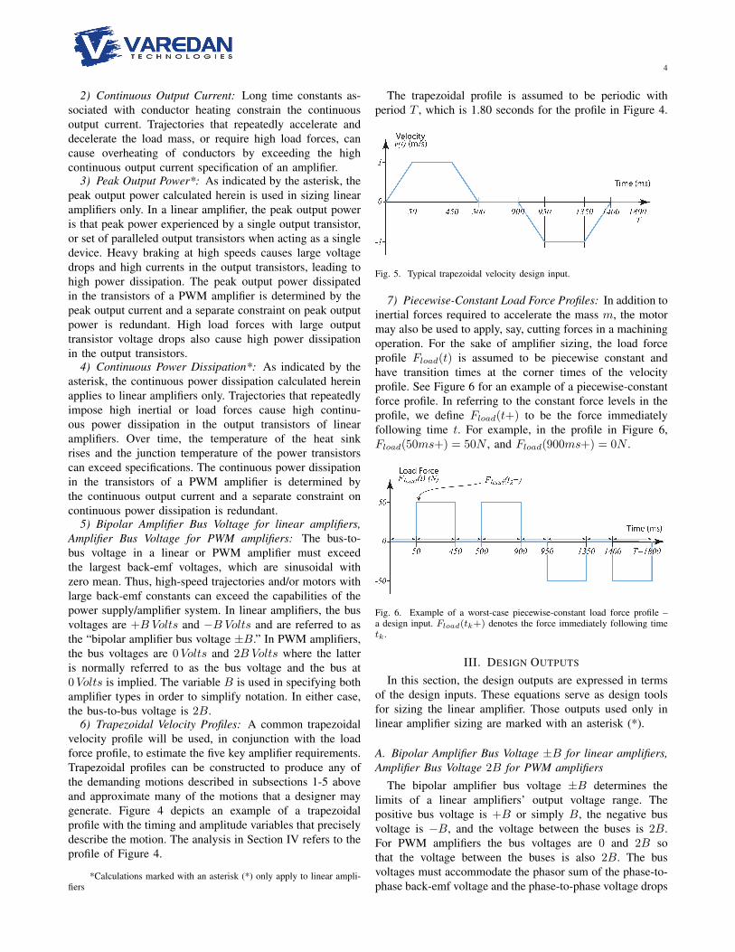
6) Trapezoidal Velocity Profiles: A common trapezoidalvelocity profile will be used, in conjunction with the loadforce profile, to estimate the five key amplifier requirements.Trapezoidal profiles can be constructed to produce any ofthe demanding motions described in subsections 1-5 aboveand approximate many of the motions that a designer maygenerate. Figure 4 depicts an example of a trapezoidalprofile with the timing and amplitude variables that preciselydescribe the motion. The analysis in Section IV refers to theprofile of Figure 4.

*Calculations marked with an asterisk (*) only apply to linear ampli-fiers

The trapezoidal profile is assumed to be periodic withperiod T , which is 1.80 seconds for the profile in Figure 4.

Fig. 5. Typical trapezoidal velocity design input.

7) Piecewise-Constant Load Force Profiles: In addition toinertial forces required to accelerate the mass m, the motormay also be used to apply, say, cutting forces in a machiningoperation. For the sake of amplifier sizing, the load forceprofile Fload(t) is assumed to be piecewise constant andhave transition times at the corner times of the velocityprofile. See Figure 6 for an example of a piecewise-constantforce profile. In referring to the constant force levels in theprofile, we define Fload(t+) to be the force immediatelyfollowing time t. For example, in the profile in Figure 6,Fload(50ms+) = 50N , and Fload(900ms+) = 0N .

Fig. 6. Example of a worst-case piecewise-constant load force profile –a design input. Fload(tk+) denotes the force immediately following timetk .

III. DESIGN OUTPUTS

In this section, the design outputs are expressed in termsof the design inputs. These equations serve as design toolsfor sizing the linear amplifier. Those outputs used only inlinear amplifier sizing are marked with an asterisk (*).

A. Bipolar Amplifier Bus Voltage ±B for linear amplifiers,Amplifier Bus Voltage 2B for PWM amplifiers

The bipolar amplifier bus voltage ±B determines thelimits of a linear amplifiers’ output voltage range. Thepositive bus voltage is +B or simply B, the negative busvoltage is −B, and the voltage between the buses is 2B.For PWM amplifiers the bus voltages are 0 and 2B sothat the voltage between the buses is also 2B. The busvoltages must accommodate the phasor sum of the phase-to-phase back-emf voltage and the phase-to-phase voltage drops

5

for the phase resistance and inductance. More precisely, letmaxtx(t) denote the maximum value of the function x(t) for

the allowable values of t. The peak phase-to-neutral voltageis given by

Vφn peak =

maxt

(√2(ma(t) + Fload(t))Rφφ2Kf

+v(t)Ke√

3

)2

+

(√2π(ma(t) + Fload(t))v(t)Lφφ

pKf

)21/2

.

(4)

Since Kf is defined in terms of an rms current, a√

2 appearsin the expression above to obtain the needed peak currentvalue. Similarly, Ke is a phase-to-phase back-emf constant,and a needed phase-to-neutral value is achieved by dividingby√

3. Factors of 2 are used to convert the phase-to-phaseRφφ and Lφφ to phase-to-neutral values.

A margin of safety of, say, 20% is often included toaccount for variation in the line voltage and for otheruncertainties. Thus, the bipolar amplifier bus voltage for alinear amplifier might be chosen to be

±B = ±1.2Vφn peak. (5)

The corresponding bus voltage for a PWM amplifierwould be

Vbus = 2B = 2.4Vφn peak. (6)

B. Peak Output Current IpeakThe peak output current is defined as the maximum value

of any phase current over the duration of a motion profile.The peak output current is given by

Ipeak ≡maxt

√2|F (t)|/Kf

= maxt

√2|ma(t) + Fload(t)|/Kf (7)

where | · | denotes absolute value and the expression in thesecond line of Equation 7 is in terms of the design inputsalone as desired.

C. Continuous Output Current IcontLong-time-constant thermal limits of conductors and other

components affect the maximum continuous output currentthat an amplifier can supply. This specification is expressedas an rms value for one phase. Continuous operation abovethis threshold is expected to cause amplifier failures. Fornon-constant operation, the specification is interpreted as anrms current computed over a periodic velocity profile. Thatis, the “mean” in the root-mean-square current is taken overthe period T of the motion:

Icont =

(1

T

∫ T

0

(ma(t) + Fload(t)

Kf

)2

dt

)1/2

. (8)

D. Peak Output Power* PpeakFor a linear amplifier, the peak output power is defined as

the maximum instantaneous power dissipated in any singleoutput transistor, or set of paralleled transistors acting as asingle device, over the entire motion profile.

Linear amplifier output transistors have a limit on peakpower dissipation, and this limit is approached when thereis a large voltage drop across an output transistor whilea high current is passing through that transistor. Such ahigh-voltage high-current condition arises when the motorvelocity is large in magnitude, positive or negative, andthe motor aggressively brakes. In this situation, the largeback-emf and the bus voltages add constructively across theoutput transistor, and large currents are required. The phase-to-phase inductance Lφφ is neglected in the peak powercalculation and, on occasion, this approximation should bereconsidered.

Express rms currents in terms of the force F and theforce constant Kf , and express peak phase-to-phase back-emf voltages in terms of the velocity v(t) and the back-emfconstant Ke. Further, recall that 2B is the voltage across thepower supply buses. Then the power dissipated in the activetransistor in a linear amplifier at a current crest is computedto be

√2B|F |/Kf −RφφF 2/K2

f −√

2vFKe/(Kf

√3). (9)

The√

2 and√

3 appear for the same reasons noted above.Note that the third term in the equation above increases thepower dissipation if v(t) and F (t) have opposite signs asexpected. Write F (t) = ma(t)+Fload(t) and the expressionfor peak output power becomes, in terms of design inputsand the design output B,

Ppeak = maxt

[√2B|ma(t) + Fload(t)|/Kf

−Rφφ(ma(t) + Fload(t))2/K2

f

−√

2v(t)(ma(t) + Fload(t))Ke/(Kf

√3)]. (10)

For the simple trapezoidal velocity profile in Figure 5, thepeak output power occurs at the beginning of the brakingperiods just following the t = 450ms and t = 1350mspoints.

This peak output power calculation only applies to linearamplifiers.

1) Frequency Adjustments to Peak Output Power*: Forshort current pulses in linear amplifiers, the thermal massof the transistor junction and surrounding silicon lowers thepeak junction temperature relative to that for a DC current ofthe same magnitude. This beneficial frequency dependence

6

is quantified in the Transient Thermal Impedance for thetransistor. For the devices used in Varedan amplifiers, thethermal mass effects are insignificant at commutation fre-quencies of about 5/3 Hz and below. However, the effectsare significant at 10Hz and above and can be exploited toachieve higher peak output power. Varedan does exploit thethermal mass effects when computing the safe operating area(SOA) of its linear amplifiers in order to avoid unnecessaryfault conditions. Further, the thermal mass effects can beused in sizing amplifiers. Using the commutation frequencyf = v/p, the junction-to-heat-sink thermal impedance forthe MOSFET is conservatively approximated by

Rj−HS(f) = 10

(0.08657 ln

(500

f

)−1.021

)+ 0.05

C

W, (11)

for f ≥ 5/3. For f < 5/3, the impedance is constantand given by Rj−HS(f) = Rj−HS(5/3). Thus, 5/3 Hzis a corner in the frequency response estimate. Define thenormalized response function as

n(f) ≡ Rj−HS(f)/Rj−HS(5/3), (12)

which is equal to 1 for frequencies below 5/3 Hz and isless than 1 for frequencies above 5/3 Hz. The normalizedresponse function n(f) is used as a scale-factor to multiplythe expression for Ppeak in Equation (9) when comparingapplication requirements to the DC peak power specified fora given linear amplifier. Interestingly, this normalization canbe used for all MOSFETs in the power range of Varedan’sproducts. This is likely due to the thermal properties ofsilicon and similarities in the device geometries. This factoronly applies to linear amplifiers and is not included in thestandard spreadsheet [1].

E. Continuous Power Dissipation* Pcont

The continuous power dissipation in the output transistorsof linear amplifiers has the potential to overheat the heatsink system and the transistor junctions. The average, overone commutation cycle, of the dissipation in the two outputtransistors of a single phase is given by

2√

2

πKf|F |B − RφφF

2

2K2f

− vFKe√6Kf

. (13)

Since the thermal time constant of the heat sink is long, thecontinuous power dissipation for a periodic velocity profilev(t) is taken to be the average over the period T of the powerdissipated in the three output stages. Using F = ma+Fload,one obtains

Pcont =3

T

∫ T

0

(2√

2

πKf|ma(t) + Fload(t)|B

− Rφφ(ma(t) + Fload(t))2

2K2f

(14)

− v(t)(ma(t) + Fload(t))Ke√6Kf

)dt.

The continuous power dissipation calculation only appliesto linear amplifiers.

IV. EVALUATING THE DESIGN OUTPUTS FORTRAPEZOIDAL VELOCITY PROFILES AND

PIECEWISE-CONSTANT LOAD FORCE PROFILES

Note that a trapezoidal velocity profile is equivalent to apiecewise-constant acceleration and load force profile. In thiscase, the design equations simplify and a systematic designprocess can be implemented in the companion spreadsheet[1]. Refer to the periodic trapezoidal velocity profile inFigure 5 and note that the profile can be specified by the ninecorners in the trapezoidal profile that have (time, velocity)coordinates (0s, 0m/s), (50ms, 1m/s), (450ms, 1m/s), . . . ,(1.8s, 0m/s), or, for short, (tk, ω(tk)); k = 1, 2, . . . , 9.Similarly for (tk, Fload(tk+)); k = 1, 2, . . . , 9, whereFload(tk+) denotes the load force just after the time tk.Due to discontinuities at tk, the value of the load force attk is not well defined. Again, the trajectory is assumed tobe periodic with, in the case of Figures 5 and 6, a period ofT = 1.8s.

The first observation to make is that the design outputs canbe calculated using v(t) and Fload(t) near the corner pointsof the velocity profile. Specifically, the design outputs aredetermined by the velocities v(tk), and the acceleration α(t)just before and just after each corner, which are denotedα(tk−) and α(tk+) respectively. The forces Fload(tk+)and Fload(tk−) also enter the calculations and the inertialforces due to acceleration and load forces are combinedinto a single force. Since the trajectory is periodic, theacceleration just after the 9th corner is the same as that justafter the 1st corner. That is α(t9+) = α(t1+) - similarlyF (t9+) = F (t1+). The acceleration and load forces areoften discontinuous right at the corners and not definedthere – although inductance in the motor windings and othersources of filtering will round the corners in practice.

When restricted to trapezoidal velocity and piecewiseconstant load force profiles, the five design equations aboveare simplified as follows.

A. Bus Voltages for Trapezoidal Velocity Profiles andPiecewise-Constant Load Force Profiles

The peak output voltage amongst all the profile cornersis obtained by maximizing over all values of the cornervelocities v(t), the accelerations a(tk±) just before andjust after to the corners, and F (tk±). Thus, the calculation

7

involves 8× 2 = 16 different evaluations of the peak phase-to-neutral voltage given by the expression in square bracketsbelow.

Vφn peak =

maxk,±

(√2(ma(tk±) + Fload(tk±))Rφφ2Kf

+v(tk)Ke√

3

)2

+

(√2π(ma(tk±) + Fload(tk±))v(tk)Lφφ

pKf

)21/2

.

(15)

When choosing the “+” or “-” in the maximization, one orthe other is used in place of ± in right-hand side of theequation.

Applying a recommended margin of 20% yields

±B = ±1.2Vφn peak (16)

for the bipolar amplifier bus voltage for a linear amplifier.The bus voltage for a PWM amplifier is

Vbus = 2B = 2.4Vφn peak. (17)

B. Peak Output Current for Trapezoidal Velocity Profilesand Piecewise-Constant Load Force Profiles

The relationship for the peak output current becomes

Ipeak = maxk,±

√2|ma(tk±) + Fload(tk±)|/Kf . (18)

C. Continuous Output Current for Trapezoidal Velocity Pro-files and Piecewise-Constant Load Force Profiles

The acceleration is constant between corner times in atrapezoidal velocity profile. Thus, the integral expression forthe continuous output current becomes the summation

Icont =(1

T

8∑k=1

(ma(tk+) + Fload(tk+)

Kf

)2

(tk+1 − tk)

)1/2

,

(19)

where T = t9 is the period of the velocity profile.

D. Peak Output Power* for Trapezoidal Velocity Profilesand Piecewise-Constant Load Force Profiles

The peak output power in a linear amplifier occurs justbefore or just following one of the corners so that theexpression for Ppeak becomes:

Ppeak = maxk,±

n

(v(tk)

p

)×[√

2B|ma(tk±) + Fload(tk±)|Kf

− Rφφ(ma(tk±) + Fload(tk±))2

K2f

(20)

−√

2v(tk)(ma(tk±) + Fload(tk±))Ke

Kf

√3

],

where either the “+” or the “-” is used in place of the ±symbol throughout. The normalized response function (notused in the spreadsheet [1]) is used to incorporate the benefitof the thermal mass of the transistor junctions. The peakoutput power calculation only applies to linear amplifiers.

E. Continuous Power Dissipation* for Trapezoidal VelocityProfiles and Piecewise-Constant Load Force Profiles

The acceleration and load forces are constant on intervalsfor the given profiles. Thus, integrating the expression forcontinuous power dissipation in a linear amplifier for suchprofiles yields

Pcont =3

T

8∑k=1

(2√

2

πKf|ma(tk+) + Fload(tk+)|B

− Rφφ(ma(tk+) + Fload(tk+))2

2K2f

− (v(tk) + v(tk+1))(ma(tk+) + Fload(tk+))Ke

2√

6Kf

)∆tk,

(21)

where ∆tk = (tk+1 − tk). This calculation does not applyto PWM amplifiers.

V. DESIGN CHECKS

In implementing the design equations above, there arevarious ways that errors may occur. In addition to the usualtranscription and algebraic errors, confusion may arise fromthe various definitions of force and back-emf constants, aswell as from the unit systems used. There are a couple simplechecks that are worth performing.

A.Kf

Ke=

√3

2≈ 1.22

For the definitions and SI units used herein the above rela-tionship between the force and back-emf constants holds forideal three-phase motors. Since magnetic materials exhibitnonlinearity, and the back-emf waveforms can deviate fromthe ideal sinusoids because of motor geometry, variations ofup to a few percent might be observed in some motor datasheets. However, if there is confusion in units, or confusionin the use of rms vs. peak or phase-to-phase vs. phase-to-neutral in parameter definitions, checking the ratio Kf

Kewill

reveal the error.

8

B.LφφRφφ

= τe

Motor data sheets are usually redundant in quoting re-sistance, inductance, and motor electrical time constant τe.The relationship above holds up to round-off and measure-ment error. If millihenries are used instead of henries andmilliseconds are used instead of seconds in the calculations,errors will escape detection with this check.

C.LφφRφφ

mink=1,...,8

(tk+1 − tk)

For good tracking, the electrical time constant of the motorshould be much shorter than any of the time periods definingthe trapezoidal velocity profile. This is rarely a problem, butit is easy to check.

VI. SIZING EXAMPLE

To illustrate the use of the design equations, consideran amplifier sizing process to address the following designinputs:• Motor force constant Kf = 39N/Arms• Motor phase-to-phase back-emf constant Ke =

32Vφφ peak/(m/s)• Motor phase-to-phase resistance Rφφ = 2.7 Ω• Motor phase-to-phase inductance Lφφ = 18mH• Motor pitch p = 24mm• Motor load mass M = 24.6 kg• Worst-case velocity profile v(t) given by Figure 5.• Load force profile equal to zero: Fload(t) = 0.

A. Example: Amplifier Bus Voltage

The peak output voltage occurs when acceleration andvelocity are both high. This peak occurs in the profile ofFigure 5 just prior to corner two and just prior to corner sixwhen the peak voltage reaches the same value. Thus, usingthe formula for Vφn peak and setting the load force to zero,one has:

Vφn peak =

(√2ma(t2−)Rφφ2Kf

+v(t2)Ke√

3

)2

+

(√2πma(t2−)v(t2)Lφφ

pKf

)21/2

(22)

From Figure 5, the velocity at corner two is 1m/s and the

acceleration just prior to corner two is1ms

0.050s= 20m/s2.

Thus,

Vφn peak =

[(√2 · 24.6 · 20 · 2.7/(2 · 39) + 1 · 32/

√3)2

+ (π ·√

2 · 24.6 · 20 · 1 · 0.018/(0.024 · 39))2]1/2

= 59.8V (23)

Applying a recommended margin of 20% yields, for a linearamplifier,

±B = ±71.8V. (24)

For a PWM amplifier, the bus voltage is

Vbus = 2B = 143.6V. (25)

.

B. Example: Peak Output Current

In the example, the peak current occurs at peak accelera-tion, which is equal to 20m/s2 for the profile of Figure 5.This current peak occurs during all of the velocity ramps. Inparticular, the peak occurs just following corner one, suchthat

Ipeak =

√2m|a(t1+)|

Kf=√

2 · 24.6 · 20

39= 17.8A (26)

C. Example: Continuous Output Current

The rms current has the same value of 17.8A/√

2 duringthe four 50ms (0.2s total) velocity ramps and 0A duringperiods of constant velocity. The continuous current istherefore

Icont =

(1

T

8∑k=1

(ma(tk+)

Kf

)2

(tk+1 − tk)

)1/2

=

(1

1.8

(24.6 · 20

39

)2

(0.2)

)1/2

= 4.21A (27)

D. Example: Peak Output Power*

For this example and linear amplifiers, the peak outputpower occurs just after corners three and seven, at whichpoint the power reaches the same high level. First, thecommutation frequency is computed as

f =v(t3)

p=

1

0.024= 41.7 Hz. (28)

Using this value of f, which is greater than the cornerfrequency of 5/3, one obtains

Rj−HS(41.7) = 10

(0.08657 ln

(500

41.7

)−1.021

)+ 0.05

= 0.168C/W, (29)

and

n(f) ≡ Rj−HS(7.23)

Rj−HS(5/3)= 0.816. (30)

The peak frequency-adjusted power is then computed as

*Calculations marked with an asterisk (*) only apply to linear ampli-fiers.

9

Ppeak = n(v(t3)

2πp)

[√2Bm|a(t3+)|

Kf

− Rφφ(ma(t3+))2

K2f

−√

2mv(t3)a(t3+)Ke

Kf

√3

](31)

= 0.816 ·

[√2 · 71.8 · 24.6 · 20

39

− 2.7 · 24.62 · (−20)2

392−√

2 · 24.6 · 1 · (−20) · 32

(39 ·√

3)

]= 963W (32)

This calculation applies only to linear amplifiers.

E. Example: Continuous Power Dissipation*

Finally, the continuous power dissipation formula withzero load force is

Pcont =3

T

8∑k=1

(2m√

2

πKf|a(tk+)|B − Rφφm

2a(tk+)2

2K2f

− (v(tk) + v(tk+1))ma(tk+)Ke

2√

6Kf

)∆tk, (33)

where ∆tk = tk+1 − tk. Equation (33) can be simplifiedby observing that power is dissipated during accelerationon the velocity ramps only. Further, there are two kinds oframps. There is one case in which acceleration and velocityhave the same sign and another case in which they havethe opposite signs. Thus, the continuous power dissipationcan be calculated by computing just these two cases anddoubling the result (the first factor of 2 in the equationbelow). The two cases are distinguished by different signsprior to the terms in square braces below (these termscancel):

Pcont = 2 · 3

1.8

(2 · 24.6

√2

π · 39· 20 · 71.8

− 2.7 · 24.62 · 202

2 · 392

−

[√2 · 24.6 · (0.5) · 20 · 32

2√

3 · 39

])(0.050)

+

(2 · 24.6

√2

π · 39· 20 · 51.2 − 2.7 · 24.62 · 202

2 · 392

+

[√2 · 24.6 · (0.5) · 20 · 32

2√

3 · 39

])(0.050)

= 200W (34)

This calculation applies to linear amplifiers only.

VII. POWER SUPPLY SIZING & MOTOR OHMIC HEATING

The primary objective of this application note is to providerequirements for choosing an amplifier. It is possible, inaddition, to compute power supply requirements and motorheat dissipation requirements, since these additional require-ments can be determined from the same design inputs usedin the amplifier sizing equations.

A. Power Supply Sizing

For a linear amplifier, the averaged absolute value of aphase current over one commutation cycle is the peak currentdivided by π/2. The worst-case power over one commuta-tion cycle into each phase amplifier is then 2BIpeak/π, andfor all three phases one has 6BIpeak/π. Since the powersupply is bipolar for linear amplifiers, the power per bus ishalf the total or

Pbus linear = 3BIpeak/π. (35)

The current per bus is

Ibus linear = 3Ipeak/π. (36)

For a PWM amplifier, the power delivered on the singlebus of voltage 2B is the same as the power delivered by thetwo buses of voltage ±B to a linear amplifier. Thus,

Pbus PWM = 6BIpeak/π. (37)

Dividing by the bus voltage 2B for a PWM amplifier, onefinds that the current requirement for a PWM amplifier isthe same as that for a linear amplifier:

Ibus PWM = 3Ipeak/π. (38)

B. Motor Ohmic Heating Pmotor−heat

The power input to the motor is converted to power outputin the form of either mechanical power in the motor shaft orheat that must be transferred from the motor to the ambientenvironment. The dominant source of heat generated in themotor is the I2R losses in the three windings, which aregiven by

Pmotor−heat =3

2I2contRφφ. (39)

The division by 2 converts the phase-to-phase resistanceRφφ to the phase-to-neutral value. There are other sourcesof heat generation in a motor associated with eddy-currents,windage, friction, and hysteresis losses in motor. Whilethese sources are generally negligible in a conservativethermal design, they can be included by adding power lossesassociated with viscous and Coulomb friction losses listedin the data sheet. Eddy-currents contribute to viscous losses,and hysteresis is usually lumped with friction measurements.

10

VIII. CONCLUSION

The equations of Section IV provide a simple means tosize linear and PWM amplifiers for driving LBMs. As notedabove, the peak output power and continuous power dissipa-tion calculations apply only to the sizing of linear amplifiers,which is indicated with an asterisk (*) throughout. In manyapplications, S-curves rather than lines define accelerations.The rounding of the corners by using such S-curves reducesthe demand on the amplifiers. If one is attempting a closefit of the motion requirement to the amplifier specification,a more complete simulation (e.g. in Matlab) will providemore information. In the case of S-curves, the equationsof Section III can be used. Such a simulation can easilyincorporate some of the inductance modeling omitted herein.Finally, care should be taken with long-period motionsand aperiodic motions, as an assumption was made thatthe thermal time-constant (∼ 60 seconds) of the heat sinksystems is long enough that the heat sink temperature isconstant and determined by Pcont.

Questions and feedback on this application note are mostwelcome and can be directed to Varedan via email atsales@varedan.com.

REFERENCES

[1] “Spreadsheet: Sizing Linear and PWM Amplifiers Driving a LinearBrushless Motor,” Varedan Technologies Document 4083-42-001.

[2] Hurley Gill, “Servomotor Parameters and their Proper Conversions forServo Drive Utilization and Comparison,” Kollmorgen Inc.