scottish institute for research in economics

SIRE DISCUSSION PAPER

SIRE-DP-2009-39

Structural Interactions in Spatial Panels

Arnab Bhattacharjee

University of St Andrews

Sean Holly

University of Cambridge

and University of St Andrews

www.sire.ac.uk

brought to you by COREView metadata, citation and similar papers at core.ac.uk

provided by SIRE

CASTLECLIFFE, SCHOOL OF ECONOMICS & FINANCE, UNIVERSITY OF ST ANDREWS, KY16 9ALTEL: +44 (0)1334 462445 FAX: +44 (0)1334 462444 EMAIL: cdma@st-andrews.ac.uk

www.st-andrews.ac.uk/cdma

Structural Interactions in Spatial Panels*

Arnab BhattacharjeeUniversity of St Andrews

Sean HollyUniversity of Cambridge

and University of St Andrews

JULY 29, 2009

ABSTRACT

Until recently, much effort has been devoted to the estimation of panel dataregression models without adequate attention being paid to the drivers of diffusionand interaction across cross section and spatial units. We discuss some newmethodologies in this emerging area and demonstrate their use in measurementand inferences on cross section and spatial interactions. Specifically, wehighlight the important distinction between spatial dependence driven byunobserved common factors and those based on a spatial weights matrix. Weargue that, purely factor driven models of spatial dependence may be somewhatinadequate because of their connection with the exchangeability assumption.Limitations and potential enhancements of the existing methods arediscussed, and several directions for new research are highlighted.

JEL Classification: E42, E43, E50, E58.

Keywords: Cross Sectional and Spatial Dependence, Spatial Weights Matrix,Interactions and Diffusion, Monetary Policy Committee, Generalised Method ofMoments.

*Correspondence: A. Bhattacharjee, School of Economics and Finance, University of St. Andrews,

Castlecliffe, The Scores, St. Andrews KY16 9AL, UK; Tel.: +44 (0)1334 462423; Fax: +44 (0)1334 462444; e-

mail: ab102@st-andrews.ac.uk.

1 Introduction1

Spatial or cross-section dependence is a common feature of most economicapplications involving either a cross-section of economic agents or a macro-economic panel of data. Increasing availability of data on spatial panels pro-vides an opportunity to understand and model such cross-section and spatialdependence. Two distinct econometric approaches have been proposed inthe literature. The …rst approach, originally developed in the regional sci-ence and geography literatures, but with increasing economic applications,is based on a spatial weights matrix, where the elements of this matrix rep-resent the direction and strength of spillovers between each pair of units.The second approach, adopts a multifactor method where it is assumed thatcross section dependence can be captured by a …nite number of unobservedcommon factors that a¤ect all units (regions, economic agents, etc.). Thispaper provides a contribution as to which of these two approaches is moreconvenient and useful in applied studies.2 In particular, we argue that spatialweights matrices with relatively unrestricted interactions are more appropri-ate in applications where spatial dependence is structural, in the sense thatthe observation units are not ‘exchangeable’.3 In other words, spatial de-pendence is driven, at least partially, by the location of the units in someobserved (or even, notional or abstract) space. Furthermore, we discuss sev-eral new econometric methods for inference on spatial dependence in theabove setting, and illustrate their relative merits based on an application tocross-member interactions within a committee.

1The paper has bene…ted from comments by Jushan Bai, Badi Baltagi, Vasco Car-valho, George Evans, Bernie Fingleton, Fritz Schueren and Je¤rey Wooldridge, as wellas participants at the International Panel Data Conference (Bonn, 2009), NTTS Con-ference (European Commission, Brussels, 2009) and seminars at Durham University andUniversity of St Andrews. The usual disclaimer applies.

2In an invited session in honour of Cheng Hsiao at the recently concluded 15 In-ternational Panel Data Conference (Bonn, 2009), Badi H Baltagi provided an extensivereview of the current literature on "Spatial Panels". Two important questions were ac-tively debated in the general discussions following the talk. First, how useful is explicitmodeling of spatial dependence using spatial weights matrices? Second, do multifactoraproaches provide more versatility in such modeling, and are there substantial advantagesof interpretability attached to spatial weights matrices? The current paper touches onboth these questions.

3The notion of exchangeability was …rst introduced by de Finetti (1937). See alsoHewitt and Savage(1955) and Gulliksen (1968).

2

The idea behind a spatial weights matrix approach is that there arespillover e¤ects across economic agents because of spatial or other formsof local cross section dependence. Such a matrix, W , is square ( £ ) withzero diagonal elements, and where the o¤-diagonal elements represent thespillover from unit to unit ( = 1 ). Panel data regression mod-els with such spatially correlated error structures have been estimated usingmaximum likelihood techniques (Anselin, 1988; Baltagi et al., 2006; Kapooret al., 2007), or generalized method of moments (Kelejian and Prucha, 1999;Conley, 1999; Fingleton, 2007). Kelejian and Prucha (2007) also extend theGMM methodology to nonparametric estimation of a heteroscedasticity andautocorrelation consistent cross section covariance matrix, for applicationswhere an instrumental variable procedure has been used to estimate the re-gression coe¢cients.

At the same time as spatial weights characterise cross section dependencein useful ways, their measurement has a signi…cant e¤ect on the estimationof a spatial dependence model (Anselin, 2002; Fingleton, 2003). Measure-ment is typically based on an underlying notion of distance between crosssection units. These di¤er widely across applications, depending not only onthe speci…c economic context but also on availability of data. Spatial conti-guity (resting upon implicit assumptions about contagious processes) usinga binary representation is a frequent choice. Further, in many applications,there are multiple possible choices and substantial uncertainty regarding theappropriate choice of distance measure. However, while the existing litera-ture contains an implicit acknowledgment of these problems, most empiricalstudies treat spatial dependence in a super…cial manner assuming in‡exibledi¤usion processes in terms of known, …xed and arbitrary spatial weightsmatrices (Giacomini and Granger, 2004). The problem of choosing spatialweights becomes a key issue in many economic applications; apart from ge-ographic distances, notions of economic distance (Conley, 1999; Pesaran etal., 2004, Holly et al., 2006), socio-cultural distance (Conley and Topa, 2002;Bhattacharjee and Jensen-Butler, 2005), and transportation costs and time(Gibbons and Machin, 2005; Bhattacharjee and Jensen-Butler, 2005) havebeen highlighted in the literature. The uncertainty regarding the choice ofmetric space and location, closely related to the measurement of spatialweights, have been addressed in the literature (Conley and Topa, 2002, 2003;Conley and Molinari, 2007). Related issues regarding endogeneity of loca-tions have also been addressed (Pinkse et al., 2002; Kelejian and Prucha,2004; Pesaran and Tosetti, 2007).

3

On the other end, spatial panel regression models under multifactor errorstructures have been addressed by maximum likelihood (Bai, 2009), prin-cipal component analysis (Coakley et al., 2006), or the common correlatede¤ects approach (Pesaran, 2006). Factor models are potentially powerful inthat they do not require strong and unveri…able a priori assumptions on thenature of spatial dependence. However, there are two potential limitations.First, a factor representation is equivalent to exchangebility of the observa-tion units, which is not a reasonable assumption in many applications. Forexample, in many spatial applications, the location of the units in space playsa key role in modelling and interpretation, and these units cannot thereforebe assumed to be exchangeable. In this paper, we use the term structuralspatial dependence to describe situations where a factor representation doesnot provide an adequate description of spatial dependence, or in other words,the observation units are not exchangeable. Second, even when an approx-imate factor representation can be obtained, it is often the case that theidenti…ed factors cannot be related in any satistactory way to interpretableindividual features or time e¤ects. Thus, economic interpretation of factormodels is often a considerable challenge.

The above two characterisations of cross section dependence, namely spa-tial weights and common factors, are not mutually exclusive. As discussedabove, factor models typically only provide a partial expanation for crosssection dependence, and therefore it is often observed that residuals fromestimated factor models display substantial cross section correlation (Hollyet al., 2006). Furthermore, Pesaran and Tosetti (2007) consider a panel datamodel where both sources of cross section dependence exist and show that,under certain restrictions on the nature of dependence, the common corre-lated e¤ects approach (Pesaran, 2006) still works.

While the above literature addressed cross section dependence in variousways, it has focused mainly on estimation of the regression coe¢cients in theunderlying model, treating the cross section dependence as a nuisance para-meter. Estimation and inferences on the magnitude and strength of spilloversand interactions has been largely ignored. However, there are many instancesin which inferences about the nature of the interaction is of independent in-terest. For example, understanding empirically the precise form of spilloversand di¤usion between observational units is an important objective of thestudies on economic growth and convergence in a cross-country panel set-ting. Likewise, studying cross-member interactions in a commitee or networksetting is a crucial counterpart to the development of theories of economic

4

networks; see, for example, Dutta and Jackson (2003) and Goyal (2007). Theempirical contribution of this paper will be based on an application of thesecond kind.

By contrast to the above literature, we take a nonparametric view onthe nature and strength of spatial di¤usion and cross section interaction.We focus explicitly on several new methods for estimating spatial weights(or interactions) that are consistent with an observed pattern of spatial (orcross sectional) dependence. Once these interactions have been estimatedthey can be subjected to interpretation in order to identify the true natureof spatial dependence, representing a signi…cant departure from the usualpractice of assuming a priori the nature of spatial interactions. The methodsare illustrated with an application to monetary policy making within theBank of England’s monetary policy committee (MPC).

The paper is organised as follows. In Section 2, we describe our modeland the econometric methods we adopt. First, we follow Bhattacharjee andJensen-Butler (2005) and describe estimation of the spatial weights matrixin a spatial error model. We emphasize that estimation of spatial weightsconsistent with an estimated pattern of spatial autocorrelations is a par-tially identi…ed problem, and therefore structural constaints are required forprecise estimation; symmetry of the spatial weights matrix constitutes sucha valid set of identifying restrictions. Second, based on Bhattacharjee andHolly (2008a), we consider estimation and inference on interactions undermoment restrictions which exploit, explicitly, the spatio-temporal nature ofpanel data on economic agents. Third, we extend the above methods toallow for spatial e¤ects that may be partly driven by unobserved commonfactors. Following this (Section 4), we develop an application to decisionmaking within the MPC, where members are allowed to have unrestrictedinteractions. Our empirical analysis illustrates each of the above methodsand further, provides interesting inferences for spatial dynamics within acommittee setting. Finally, Section 5 concludes, highlighting strengths andweaknesses of the methods we have used, as well as suggesting possible areasof new research.

2 Model and methodologies

The spatial weights matrix is one of the most convenient ways to summarisespatial relationships in the data. With conventional geographical data, the

5

spatial weights matrix re‡ects the intensity of the geo-spatial relationshipbetween observations in a neighbourhood, for example, contiguity, the dis-tances between neighbours, the lengths of shared border, or whether theyfall into a speci…ed directional class such as north/ south. Standard spa-tial autocorrelation statistics compare the spatial weights to the covariancerelationship at pairs of locations. Spatial autocorrelation that is more posi-tive than expected from random assignment indicate the clustering of similarvalues across geo-space, while signi…cant negative spatial autocorrelation in-dicates that neighboring values are more dissimilar than expected by chance.

Since spatial weights are usually de…ned by conventional measures of ge-ographic (or economic) distances between observation units, or various mea-sures of contiguity, a spatial weights matrix is typically a exogenous (andknown) square matrix with zero diagonal elements and positive symmetricelements away from the diagonal. Given a spatial weights matrix W , dy-namic spatial regression models are constructed in ways analogous to stan-dard time series analysis, with the spatial lag of a vector of observationsfor all units de…ned as the vector W . Once such a regression model hasbeen set up, inferences can be drawn using a variety of methods, includingmaximum likelihood and GMM; see, for example, Anselin (1999) and Anselinet al. (2003) for further discussion.

However, as discussed earlier, there is in most real applications consider-able uncertainty regarding measurement of these distances. Worse still, infer-ences drawn using mis-measured spatial weights are typically biased (Anselin,2002; Fingleton, 2003) and further, inferences from mis-speci…ed spatial mod-els are also inadequate (Baltagi et al., 2007). Thus, while convential spatialeconometric methods have treated the spatial weights as known, estimationof the spatial weights matrix is emerging as an important and active area ofresearch (Dubin, 2009).

2.1 Spatial error model with unrestricted structural

dependence

Studies in spatial econometrics typically distinguish between two kinds ofspatial e¤ects in regression models for cross-sectional and panel data – spa-tial interaction (spatial autocorrelation) and spatial structure (spatial het-erogeneity). While the study of spatial structure is similar to the traditionaltreatment of coe¢cient heterogeneity in econometrics, spatial interaction is

6

usually modeled through a spatial weights matrix. Given a particular choiceof the spatial weights matrix, there are two important and distinct waysin which spatial interaction is modelled in spatial regression analysis – thespatial error model and the spatial lag model.

We consider the spatial error model with spatial autoregressive errors,where the vector response variable () is explained by the e¤ects of explana-tory variables (X) and spatial spillover of errors from other units.4 Themodel and its reduced form are described as follows:

= X + = 1 (1)

= W + (2)

=) = X + (I ¡ W )¡1

where there are time periods ( = 1 ) and units ( = 1 ). is

the £1 vector of the response variable in period , W is an unknown spatialweights matrix of dimension £, and is the £ 1 vector of independentbut possibly heteroscedastic spatial errors.

We …rst make the following four assumptions.Assumption 1: We assume that the spatial errors, , are iid (independentand identically distributed) across time. However, we allow for heteroscedas-ticity across regions, so that E (

0) = § = (21

22

2), and 2 0

for all = 1 .The uncorrelatedness of the spatial errors across the units is crucial. As-

sumption 1 ensures that all spatial autocorrelation in the model is solelydue to spatial di¤usion described by the spatial weights matrix.Assumption 2: The spatial weights matrix W is unknown and possiblyasymmetric. W has zero diagonal elements and there are no restrictions onthe o¤-diagonal elements (i.e., they could be either positive or negative).

For the moment, we retain the ‡exibility of a possibly asymmetric spatialweights matrix. Our most signi…cant point of departure from the literatureis in the assumption of an unknown spatial weights matrix, which we intendto conduct inferences on. We do not impose a non-negativity constraint onthe o¤-diagonal elements of W .Assumption 3: (I ¡ W ) is non-singular, where I is the identity matrix.This is a standard assumption in the literature, and required for identi…cationin the reduced form.

4By contrast, the spatial lag model includes the spatial lag of the response variable,W, as an additional regressor.

7

Under Assumption 3, we have:

E (0) = (I ¡ W )¡1 § (I ¡ W )¡10

2.2 Exchangeability and the multifactor model

As emphasized above, we will focus on the situation where spatial depen-dence is structural. In other words, we do not make an assumption that themultifactor model holds. Here, we argue that such an assumption may bestrong and unsatisfactory when the objective is to infer on the strength ofspatial interactions. In particular, we discuss the link between the multifac-tor representation and exchangeability and emphasize that exchangeabilityof the spatial units is not a particularly useful assumption in our setting.

De…nition: An exchangeable sequence of random variables is a …nite or in-…nite sequence 1 2 3 of random variables such that for any …nitepermutation of the indices 1 2 3 , that is, any permutation that leavesall but …nitely many indices …xed, the joint probability distribution of thepermuted sequence (1) (2) (3) is the same as the joint probabilitydistribution of the original sequence.

Originally proposed by de Finetti (1937), the idea of exchangeability wasfurther developed by Hewitt and Savage (1955). Exchangeability is somewhatsimilar to, but a weaker notion of IID-ness. The idea that measurements forthe same attribute should be exchangeable, and therefore a link between ex-changeability and an underlying single factor model, dates back to Gulliksen(1968). However, the exact nature of this link has been unclear, and is atopic of considerable current research interest.

Kelderman (2004) shows that the Gaussian single factor model is ex-changeable. His setting considers multiple exchangeable ratings providingdi¤erent measurements on the same attribute, this attribute being the latentfactor. In our spatial setting, this corresponds to the question as to whetherelements of are exchangeable, or in other words, whether their speci…cspatial identity does not matter. If the units are exchangeable, and they areGaussian, the results of Kelderman (2004) imply that a single factor modelwould provide adequate representation for spatial dependence.

Forni et al. (2004) provide a characterization for the more general dy-namic factor model. Their work emphasizes a crucial assumption (Assump-tion (R), Forni et al. (2004), p.239), whose general intuition and treatment

8

is yet to be fully understood. However, in the spatial setting where thecross-sectional dimension is ‘not well-ordered’, the assumption implies ‘somekind of "cross-sectional exchangeability"’ (Forni et al., 2004, p.240). In otherwords, a major case in which the generalised factor model provides consistentinferences is one where the spatial, or cross-section, units are exchangeable.

Andrews (2005) develops inference for cross-section regression with com-mon shocks. Although not speci…c to the panel setting, the work demon-strates some important implications for the multifactor model. Speci…cally,regression provides valid inferences under sampling schemes where, condi-tional on a -…eld generated by the common shocks (or factors), the ob-servations are exchangeable (Assumption 1, Andrews (2005), p. 1555). Healso argues that this setting and assumptions are very general. Importantlyfor our current problem, he also discusses extensions to heterogenous factorstructures and to the panel regression model with …xed .

The above literature points to the general idea that exchangeability isclosely linked with the multifactor model. However, our inference problemhere concerns cross-section interactions rather than estimation of the un-derlying regression model itself. Hence, even though the exchangeabilityassumption may be reasonably meaningful in the regression setting, it is notparticularly useful in our setting. Speci…cally, if we assume some form ofexchangeability for the spatial units, each individual observation unit losesits speci…c identity, and therefore the question of inference of interactions be-comes meaningless. This is in addition to the fact that, in …nite situations,exchangeability may itself be a tenuous assumption. Hence, we do not makethe exchangeability assumption, and retain the ‡exibility that the structuraldependence model o¤ers.

2.3 Estimation under structural constraints

Under the structural dependence assumption, Bhattacharjee and Jensen-Butler (2005) consider estimation of a spatial weights matrix in the spa-tial error model with spatial autoregressive errors (1, 2). They consider asetting where a given set of cross section units have …xed but unrestrictedinteractions; these interactions are inherently structural in that the units arenot exchangeable, and the interactions are therefore related to an underly-ing structural economic model. In addition to Assumptions 1-3 above, theymake the following assumption.

9

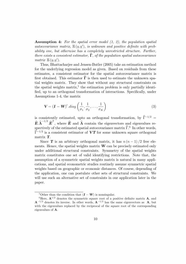
Assumption 4: For the spatial error model (1, 2), the population spatialautocovariance matrix, E (0), is unknown and positive de…nite with prob-ability one, but otherwise has a completely unrestricted structure. Further,there exists a consistent estimator, b¡, of the population spatial autocovariancematrix E (0).

Thus, Bhattacharjee and Jensen-Butler (2005) take an estimation methodfor the underlying regression model as given. Based on residuals from theseestimates, a consistent estimator for the spatial autocovariance matrix is…rst obtained. This estimator b¡ is then used to estimate the unknown spa-tial weights matrix. They show that without any structural constraints onthe spatial weights matrix,5 the estimation problem is only partially identi-…ed, up to an orthogonal transformation of interactions. Speci…cally, underAssumptions 1-4, the matrix

V = (I ¡ W )0

µ1

11

2

1

¶

(3)

is consistently estimated, upto an orthogonal transformation, by b¡¡12 =bEb¤

¡12bE

, where bE and b¤ contain the eigenvectors and eigenvalues re-

spectively of the estimated spatial autocovariance matrix b¡.6 In other words,b¡¡12 is a consistent estimator of V T for some unknown square orthogonalmatrix T .

Since T is an arbitrary orthogonal matrix, it has ( ¡ 1) 2 free ele-ments. Hence, the spatial weights matrix W can be precisely estimated onlyunder additional structural constraints. Symmetry of the spatial weightsmatrix constitutes one set of valid identifying restrictions. Note that, theassumption of a symmetric spatial weights matrix is natural in many appli-cations, and spatial econometric studies routinely assume symmetric spatialweights based on geographic or economic distances. Of course, depending ofthe application, one can postulate other sets of structural constraints. Wewill use such an alternative set of constraints in our application later in thepaper.

5Other than the condition that (I ¡ W ) is nonsingular.6Here, A12 denotes the symmetric square root of a positive de…nite matrix A, and

A¡12 denotes its inverse. In other words, A¡12 has the same eigenvectors as A, butwith the eigenvalues replaced by the reciprocal of the square root of the correspondingeigenvalues of A.

10

Under the above structural assumptions, Bhattacharjee and Jensen-Butler(2005) describe inference methods and an algorithm for estimation of the un-known spatial weights matrix. Estimation requires application of the “gra-dient projection” algorithm (Jennrich, 2001) which optimises any objectivefunction over the group of orthogonal transformations of a given matrix.Convergence is fast and the algorithm is easily programmable.7

However, the above method has two important limitations. First, theidentifying restrictions of symmetry (or other alternate structural assump-tions) may be too strong in some applications. Second, and more importantly,these structural constraints are not generally testable. Further, standard er-rors in the above method have to be estimated by a bootstrap procedurewhich can be computation intensive.

2.4 GMM based inferences on endogenous interactions

In the same setting as above, Bhattacharjee and Holly (2008a) developedan alternative GMM based methodology for estimating spatial or interactionweights matrices which are unrestricted except for the validity of the includedinstruments and other moment conditions. This method assumes a nonemptyset of other cross section units, correlated with the units under consideration,but which may change over time, expand or even vanish. Speci…cally, mo-tivated by the system GMM approach (Arellano and Bond, 1991; Blundelland Bond (1998), they use these additional cross section (or spatial) unitsto constitute instruments, in addition to temporal lags normally available asinstruments in a panel data setting. Bhattacharjee and Holly (2008a) alsoextend their methodology to a model with interval censored responses.

Like Bhattacharjee and Jensen-Butler (2005), the methodology in Bhat-tacharjee and Holly (2008a) relies on an estimator for the underlying regres-sion model

= X +

Residuals, e, from this estimated model are …rst obtained. Then, for a givencross section unit , the following regression model in latent errors follows

e = e 0(¡)() +

7An implementation of the algorithm in Matlab is available from the authors on request.

11

where e(¡) denotes the vector of residuals for the cross section units otherthan , () is the -th row of W transposed (ignoring the diagonal element,which is zero by assumption), and observations run over = 1 . Ateach subsequent estimation step, they estimate (), an index row of W . Thesame procedure is repeated for each cross section unit in turn, and the wholeW matrix is therefore estimated.

The main issue with the estimation of the above model is the endogene-ity of the regressors, e(¡). In order to address this issue, Bhattacharjeeand Holly (2008a) draw on the connection between the setting here and thestandard dynamic panel data model. Here, we have (spatially) lagged en-dogenous variables as regressors, but the observations are not sampled atequi-spaced points on the time axis. Rather, the locations of our units lie ina multi-dimensional, and possibly abstract, space without any clear notion ofordering or spacing between observations. At the same time, one can oftenimagine that potential nonzero interaction weights imply that 1 2 are regression errors from (1), at time , on a collection of observation unitswho are not located very far away in space. In many applications, theremay also be, potentially speci…c to the time period, additional units who arelocated further away (like those at higher lags in the dynamic panel datamodel), who are correlated with the above set of endogenous variables, butnot with the idiosyncratic errors 1 2 from the interaction errorequation (2).

In social networks agents who have weak ties with other agents may actas instruments for groups of agents that share strong ties (Granovetter, 1973,Goyal, 2007). In panel data on cross-sections of countries or regions, such aset may include other countries not included in the analysis either becauseof irregular availability of data or because they are outside the purview ofthe analysis. Similarly, in geography and regional studies, observations at a…ner spatial scale may constitute such instruments.Assumption 5: There is, speci…c to a particular time point , a collection of

instruments () =

³(1)

(2)

()

´, with corresponding

P=1 moment

conditions

³()

´= 0 = 1 2 ; = 1 2 (4)

The validity of these potentially large number of instruments can bechecked using, for example, the Sargan-Hansen -test (Hansen, 1982). How-ever, weak instruments may also potentially provide a problem here. Simi-

12

lar to Arellano and Bond (1991), and assuming a …rst order autoregressivestructure in the errors of the interactions model, a further set of momentconditions are obtained.Assumption 6: Assume a …rst order autoregressive model

= ¡1 + = 1 2 ; = 2 3

() = 0 6=

so that an additional ( ¡ 1) ( ¡ 2) 2 linear moment conditions follow

¡(¡2)

¢= 0 = 3 (5)

where (¡2) =³(¡2)1

(¡2)2

(¡2)

´and

(¡2) = (1 2 ¡2) for

= 1 2 .Estimation can now follow along standard lines. First, we estimate the

underlying regression model (1) using an optimisation based method suchas maximum likelihood, least squares or GMM, and collect residuals. Next,we estimate the interactions error model (2) using a two-step GMM estima-tor. The weights matrix is estimated using the outer product from momentconditions evaluated at an initial consistent estimator, which is the GMM es-timator using the identity weighting matrix. The validity of this multi-stepprocedure follows from Newey (1984).

Bhattacharjee and Holly (2008a) also extend their methodology to thecensored regression model. This is achieved by making a control functionassumption.Assumption 7: Assume the interval censored observation scheme

Observations :¡[0 1] e(¡)

¢(6)

(e 2 [0 1]) = 1

where =³() (¡2)

´is a set of instruments. Further, the following

conditions hold:

e(¡) = 0+ ; () = 0; (7)

= 0 + ; ? ; » ¡0 2

¢

The interval inequalities (e 2 [0 1]) = 1 can be expressed as

0 = 1¡¡0 + e 0

(¡)() + 0 + ¸ 0¢

and (8)

1 = 1¡1 ¡ e 0

(¡)() ¡ 0 ¡ ¸ 0¢

(9)

13

Then, assuming exogenous censoring intervals, and using the control func-tion approach (Blundell and Smith, 1986), the following moment conditionscan be obtained:

£

¡e(¡) ¡ 0

¢¤= 0

£0

¡0 0 e(¡)

¡e(¡) ¡ 0

¢

¢e(¡)

¤= 0

£0

¡0 0 e(¡)

¡e(¡) ¡ 0

¢

¢ ¡e(¡) ¡ 0

¢¤= 0 (10)

£0

¡0 0 e(¡)

¡e(¡) ¡ 0

¢

¢0

¤= 0

£1

¡1 1 e(¡)

¡e(¡) ¡ 0

¢

¢e(¡)

¤= 0

£1

¡1 1 e(¡)

¡e(¡) ¡ 0

¢

¢ ¡e(¡) ¡ 0

¢¤= 0

£1

¡1 1 e(¡)

¡e(¡) ¡ 0

¢

¢1

¤= 0

where

0¡0 0 e(¡)

¢

= 0

h³

¡0 + e 0(¡)() + 0

´

i

©h³

¡0 + e 0(¡)() + 0

´

i

+(1¡ 0)¡

h³¡0 + e 0

(¡)() + 0´

i

1¡ ©h³

¡0 + e 0(¡)() + 0

´

i , and

1¡1 1 e(¡)

¢

= 1

h³

1 ¡ e 0(¡)() ¡ 0

´

i

©h³

1 ¡ e 0(¡)() ¡ 0

´

i

+(1¡ 1)¡

h³1 ¡ e 0

(¡)() ¡ 0´

i

1¡ ©h³

1 ¡ e 0(¡)() ¡ 0

´

i

and and © are the pdf and cdf of the standard normal distribution respec-tively. As before, GMM estimation can now proceed along standard lines.

In a simple way, the above methodology exploits the panel nature ofthe data as well as spatial interactions to obtain robust inferences in the

14

presence of potential endogeneity. This is particularly important in micro-economic and spatial contexts where the positions of economic agents orregions in geographical and quality space are determined strategically, andtherefore endogenously, as a result of repeated cross section interactions; seealso Pinkse et al. (2002) and Conley and Topa (2003).

The GMM based methods discussed above are potentially quite powerful.They also have the advantage that unveri…able assumptions on the structureof W are not required. However, there may be a weak instruments model.It is an empirical question as to which sets of identifying assumptions, struc-tural restrictions as in Bhattacharjee and Jensen-Butler (2005) or momentrestrictions as in Bhattacharjee and Holly (2008a), is more appropriate inthe context of any speci…c application.

2.5 Presence of unobserved common factors

The above two methodologies are based on the structural spatial dependenceassumption that the spatial units under observation are not exchangeable.However, just as a pure factor model usually explains only a part of the spatialdependence, a pure structural dependence assumption can also be problem-atic. Such an assumption would imply that whatever structural drivers leadto spatial autocorrelation, whether geographic distance or something moreabstract, it is uncorrelated with the regressors included in the model. Thesedrivers shape a particular pattern of spatial interaction, which then a¤ectsthe spatial di¤usion of shocks, and which in turn we can identify and inferupon using the above methods. Clearly, this is a strong assumption.

Furthermore, some spatial interactions could be also driven by commonfactors, and there can be a combination of both structural drivers and un-observed factors.8 Pesaran and Tosetti (2007) consider a model where, inaddition to spatial or network interactions described by a weights matrix,there are unobserved common factors; see also Holly et al. (2006). Theirestimation is based on the common correlated e¤ects approach (Pesaran,2006) where, in addition to the usual regressors, linear combinations of un-observed factors are approximated by cross section averages of the dependentand explanatory variables. De…ning notions of weak and strong cross sectiondependence, Pesaran and Tosetti (2007) show that the common correlated

8While the literature on spatial econometrics has been silent on this crucial question,there is some discussion of related issues in the literature on regional growth and conver-gence; see, for example, Evans and Karras (1996).

15

e¤ects method provides consistent estimates of the slope coe¢cient underboth forms of dependence. Here, we are interested in inferences on spatialinteractions under the model:

= + 0 + () +

()0

+ (11)

= W + = 1 2

where our original model (1) is simply augmented with cross section averagesof and ( and respectively).

While inference in Pesaran and Tosetti (2007) assumes certain structuralconstraints on the weights matrix, our network interactions are unrestrictedexcept for the identifying assumption that the matrix (I ¡ W ) is nonsingu-lar. Instead, we would achieve identi…cation through the moment conditionsgiven in (4) and (5). Under these moment conditions, GMM estimation isstraightforward.

Also, as in the previous subsection, we can accommodate interval cen-sored responses, assuming that censoring intervals are exogenous and thenconducting GMM estimation under the moment conditions (10).

This combination of spatial weights estimation with the multifactor modelis very powerful. It will allow us to decide on the relative importance of factorbased and structural explanations of spatial dependence. Furthermore, it isnow possible to additionally infer on both the drivers of the structural spatiale¤ects as well as the endogenous network architectures.

3 Application: Interactions within the Bank

of England’s MPC

We develop the methodological approach described above in the context ofa particular form of interaction. In this case it is the decisions that a Com-mittee makes on interest rates for the conduct of monetary policy.

3.1 A simple model of committee decision making withinthe MPC

Our model for the in‡ation process is structured as follows:

= ¡1 + ¡1 + (12)

= 1¡1 ¡ 2(¡1 ¡ ¡1) + (13)

16

Here, is the in‡ation rate in period , is the output gap (the di¤erencebetween the log of output and the log of potential output), and the nominalinterest rate. , a supply shock and , a demand shock, are iid shocks inperiod not observable in period ¡1. The coe¢cients and 2 are positive;1 (0 1 1) measures the degree of persistence in the output gap. Theoutput gap depends negatively on the real lagged interest rate. The changein in‡ation depends on the lagged output gap. The output gap is normalisedto zero in the long run.

If the policymaker only targets in‡ation, the central bank can (in expec-tation) use the current interest rate to hit the target for in‡ation two periodshence. So the intertemporal problem can be written as a sequence of singleperiod problems. In this case (Svensson, 1997):

=1

2

£+2j ¡ ¤

¤2 (14)

where +2j is the forecast of in‡ation at time period + 2 based on infor-mation available in period .

Then the rule for setting the interest rate by the monetary authority is:

= j +1

2(+1j ¡ ¤) +

12

j (15)

Next, we model the decision making process within the MPC. A standardway of understanding how a committee comes to a decision is that each mem-ber reacts independently to a ‘signal’ coming from the economy and makesan appropriate decision in the light of this signal and the particular prefer-ences/expertise of the member. A voting method then generates a decisionthat is implemented. In practice there is also cross committee dependence.Before a decision is made there is a shared discussion of the state of the worldas seen by each of the members. In this section we model the possible inter-actions between members of a committee as one in which interaction occursin the form of deliberation. Views are exchanged about the interpretation ofsignals and an individual member may decide to revise his view dependingupon how much weight he places on his own and the views of others.

This process can be cast as a simple signal extraction problem withina highly stylised framework. Let the -th MPC member formulate an (un-biased) estimate of, say, the output gap, . We adopt this notation heresince we wish to consider situations where = 1 members could be

17

a subset of a Committee of members. Then the underlying model for the-th member is:

= +

with v (0 2) and (16)

¡

¢=

= for = 1

The initial estimates of the output gap for each individual member are unbi-ased. Further, since

re‡ects private views not shared by other committeemembers, we would normally expect that (

) = 0, for 6= . However,

in case there is strategic interaction between committee members and , and

can be correlated.The internal process of deliberation between the members of the Com-

mittee reveals to everyone individual views of the output gap brought to themeeting.9 At the end of discussion and deliberation, an agreed estimate, ,of the output gap is agreed upon. This common estimate ( ) is a weightedaverage of the initial estimates for the committee members, the weightsre‡ecting their relative importance or seniority within the committee. There-fore

= + with

v (0 2) (17)

is also unbiased for the unknown true output gap.For the -th member, the …nal estimate of that minimises the forecast

error variance and combines optimally the central bank estimate ( ) and theprivate estimate ( ) is given by:

= + ( ¡ ) (18)

where is:

=2

2+ 2

(19)

Clearly the more con…dent the committee member is in her own judgementthe smaller 2 , and the less weight is attached to the collective forecast.

9Austin-Smith and Banks (1996) point out that we need each committee member tobe open in revealing his estimate of the output gap and sincere in casting a vote for aninterest rate decision that corresponds to the infomation available. Although we consideronly the one period problem here, in a multi-period context we assume that reputationalconsiderations are su¢ciently powerful to ensure fair play.

18

This …nal estimate shows how members may di¤er about the size of theoutput gap. Committee members may also di¤er in their views on the e¤ectof interest rates on in‡ation and output gap. This implies member-speci…ce¤ects 2 and 2 respectively.

Then, the decision rule for the -th member can be written as:

= j +1

2(+1j ¡ ¤) +

12

j + , (20)

where j = is the average (forecast) of the current output gap, and

=12

( ¡ j) (21)

represents the e¤ect of the deviation of the -th member’s initial estimate ofoutput gap from the common estimate.

There are two important features of the ’s, which are crucial for ourempirical analysis. First, need not be a zero mean process and in generalcaptures the extent to which the -th member deviates from the centralinterest rate projection. Hence, can be expressed in …xed e¤ects form as

= +

Second, the ’s are uncorrelated across di¤erent meetings for the same pol-icy maker, but are correlated across members of the committee. This is fortwo reasons: (a) they are related to each other through the common esti-mate (j), which is a linear combination of individual estimates, and (b)there may be strategic interactions among committee members, in whichcase (

) 6= 0 for some 6= .

Therefore, our model implies the following decision rule for the -th mem-ber:

= j+1

2(+1j ¡ ¤) +

12

j+ + + + (22)

where (the …xed e¤ect) indicates whether the -th member is a hawk (high

values) or a dove, denotes indicators included in the -th member’s esti-mate of the output gap (with heterogeneity both in the choice of the variables

19

and in their e¤ects), is a measure of the uncertainty associated with thefuture macroeconomic climate and denotes the -th member’s responseto such uncertainty, and ’s are zero mean errors with heteroscedastic vari-ances across members; the magnitude of the variance re‡ects how activist aparticular member is. For member , ’s are uncorrelated across meetings.However, ’s are correlated across members, because of (a) deliberationwithin the committee, and (b) strategic interaction between members.

3.2 Data and sample period

The primary objective of the empirical study is to understand cross memberinteraction in decision making at the Bank of England’s MPC, within thecontext of the model of committee decision making presented in the previ-ous section. Importantly, our framework allows for heterogeneity among theMPC members and the limited dependent nature of preferred interest ratedecisions. Our dependent variables are the decisions of the individual mem-bers of the MPC. The source for these data are the minutes of the MPCmeetings.

TABLE 1: Voting records of selected MPC membersMember Meetings Votes Dissent

Lower No change Raise Total High Low

Buiter 36 10 10 16 17 9 8Clementi 63 14 39 10 4 3 1George 74 15 51 6 0 0 0Julius 45 18 25 2 14 0 14King 85 14 50 21 12 12 0

Since mid-1997, when data on the votes of individual members startedbeing made publicly available, the MPC has met once a month to decide onthe base rate for the next month.10 Over most of this period, the MPC hashad 9 members at any time: the Governor (of the Bank of England), 4 inter-nal members (senior sta¤ at the Bank of England) and 4 external members.External members were usually appointed for a period ranging from 3 to 4years. Because of changes in the external members, the composition of theMPC has changed reasonably frequently. To facilitate study of heterogeneity

10The MPC met twice in September 2001. The special meeting was called after theevents of 09/11.

20

and interaction within the MPC, we focus on 5 selected members, includingthe Governor, 2 internal and 2 external members. The longest such periodwhen the same 5 members have concurrently served in the MPC is the 33month period from September 1997 to May 2000. The 5 MPC members whoserved during this period are: George (the Governor), Clementi and King(the 2 internal members) and Buiter and Julius (the 2 external members).The voting pattern of these selected MPC members suggest substantial vari-ation (Table 1).11

In order to explain the observed votes of the 5 selected members, we col-lected information on the kinds of data that the MPC looked at for eachmonthly meeting. The important issue was to ensure that we conditionedonly on what information was actually available at the time of each meet-ing. Assessing monetary policy decisions in the presence of uncertainty aboutforecast levels of in‡ation and the output gap (including uncertainty both inforecast output levels and perception about potential output) requires col-lection of real-time data available to the policymakers when interest ratedecisions are made as well as measures of forecast uncertainty. This con-trasts with many studies of monetary policy which are based on realised(and subsequently revised) measures of economic activity (see Orphanides,2003).

We collected information on unemployment (where this typically refersto unemployment three months prior to the MPC meeting), as well dataon the underlying state of asset markets (housing prices, share prices andexchange rates). We measure unemployment by the year-on-year changein International Labor Organization (ILO) rate of unemployment, lagged3 months. The ILO rate of unemployment is computed using 3 monthsrolling average estimates of the number of ILO-unemployed persons and sizeof labour force (ILO de…nition), both collected from the O¢ce of NationalStatistics (ONS) Labour Force Survey. Housing prices are measured by theyear-on-year growth rates of the Nationwide housing prices index (seasonallyadjusted) for the previous month (Source: Nationwide). Share prices andexchange rates are measured by the year-on-year growth rate of the FTSE

11For example, of the 45 meetings which Julius attended, the votes for 14 were againstthe consensus decision, and all of these were for a lower interest rate. On the other hand,King disagreed with the consensus decision in 12 of the 82 meetings he attended, votingfor a higher interest rate each time. Buiter dissented in 17 meetings out of 36, voting on8 occasions for a lower interest rate and 9 times in favour of a higher one. See also King(2002) and Gerlach-Kristen (2004).

21

100 share index and the e¤ective exchange rate respectively at the end of theprevious month (Source: Bank of England). The other current informationincluded in the model is the current level of in‡ation – measured by theyear-on-year growth rate of RPIX in‡ation lagged 2 months (Source: ONS).

Our empirical model also includes expected rates of future in‡ation andforecasts of current and future output. One di¢culty with using the Bank’sforecasts of in‡ation is that they are not su¢ciently informative. By de…ni-tion, the Bank targets in‡ation over a two year horizon, so it always publishesa forecast in which (in expectation) in‡ation hits the target in two years time.To do anything else would be internally inconsistent. Instead, as a measureof future in‡ation, we use the 4 year ahead in‡ation expectations implicitin bond markets at the time of the MPC meeting, data on which can beinferred from the Bank of England’s forward yield curve estimates obtainedfrom index linked bonds.12 For current output, we use annual growth of 2-month-lagged monthly GDP published by the National Institute of Economicand Social Research (NIESR) and for one-year-ahead forecast GDP growth,we use the Bank of England’s model based mean quarterly forecasts.

Finally, uncertainty in future macroeconomic environment and privateperceptions about the importance of such uncertainty plays an importantrole in the model developed in this paper. The extent to which there isuncertainty about the forecast of the Bank of England can be inferred fromthe fan charts published in the In‡ation Report. As a measure of uncertaintyin the future macroeconomic environment, we use the standard deviation ofthe one-year-ahead forecast. These measures are obtained from the Bank ofEngland’s fan charts of output; details regarding these measures are discussedelsewhere (Britton et al., 1998).

3.3 The empirical model

We start with the model of individual voting behaviour within the MPCdeveloped in the previous section. The model includes individual speci…cheterogeneity in the …xed e¤ects, in the coe¢cients of in‡ation and outputgap, and in the e¤ect of uncertainty. We aim to estimate this model in aform where the dependent variable is the -th member’s preferred changein the (base) interest rate. In other words, our dependent variable, ,

12We use the four year expected in‡ation …gure because the two year …gure is notavailable for the entire sample period. In practice the in‡ation yield curve tends to bevery ‡at after two years.

22

represents the deviation of the preferred interest rate for the -th member(at the meeting in month ) from the current (base) rate of interest ¡1:

= ¡ ¡1

Therefore, we estimate the following empirical model of individual deci-sion making within the MPC:

= + () 4¡1 +

(0) +

(4) +4j +

(0) j (23)

+(1) +1j +

()

¡+1j

¢+

+

where represents current observations on unemployment (4) and theunderlying state of asset markets: housing, equity and the foreign exchangemarket (, and respectively). The standard deviation ofthe one-year ahead forecast of output growth is denoted by

¡+1j

¢; this

term is included to incorporate the notion that the stance of monetary policymay depend on the uncertainty relating to forecast future levels of output andin‡ation. As discussed in the previous section, increased uncertainty aboutthe current state of the economy will tend to bias policy towards caution inchanging interest rates. In particular, this strand of the literature suggeststhat optimal monetary policy may be more cautious (rather than activist)under greater uncertainty in the forecast or real-time estimates of output gapand in‡ation (see Issing, 2002; Aoki, 2003; and Orphanides, 2003). Since, aspreviously discussed, the published in‡ation forecast is not su¢ciently infor-mative, we con…ned ourselves to uncertainty relating to forecasts of futureoutput growth.

However, there are two important additional features of our data gen-erating process that render the estimation exercise nonstandard. First, thedependent variable is observed in the form of votes, which are highly clusteredinterval censored outcomes based on the underlying decision rules. Second,and importantly in our context, the regression errors are potentially interre-lated across the members. Therefore, we augment the empirical model (23)with a model for interaction between the error terms for di¤erent members

= W + (24)

where W is a ( £ ) matrix of interaction weights with zero diagonalelements and unrestricted entries on the o¤-diagonals, subject to the con-straint that (I ¡ W ) is nonsingular, and = (1 2 )

0 is a vector

23

of uncorrelated errors that are possibly heteroscedastic with

(0) = § =

2

6664

21 0 00 22 0...

.... . .

...0 0 2

3

7775

Votes of MPC members are highly clustered, with a majority of the votesproposing no change in the base rate. The …nal decisions on interest ratechanges are all similarly clustered. For the Bank of England’s MPC as awhole over the period June 1997 to March 2005, 69 per cent of the meetingsdecided to keep the base rate at its current level, 14 per cent recommendeda rise of 25 basis points, 13 per cent recommended a reduction of 25 basispoints, and the remaining 4 per cent a reduction of 50 basis points.

This clustering has to be taken into account when studying individualvotes and committee decisions of the MPC. We do not observe changes in in-terest rates on a continuous or unrestricted scale, we have a non-continuousor limited dependent variable. Moreover, changes in interest rates are inmultiples of 25 basis points. Therefore, we use an interval regression frame-work for analysis; other authors have used other limited dependent variableframeworks, like the logit/ probit or multinomial logit/ probit framework toanalyse monetary policy decisions. Our choice of model is based on the needto use all the information that is available when monetary policy decisions aremade, as well as problems relating to model speci…cation and interpretationof multinomial logit models (Greene, 1993). We also explored an ordered andmultinomial logit formulations, and found the broad empirical conclusions tobe similar.

Therefore, the observed dependent variable in our case, , is the trun-cated version of the latent policy response variable of the -th member, ,which we model as

= ¡025 if 2 [¡0375¡020)

= 0 if 2 [¡020 020] (25)

= 025 if 2 (020 0375] and

2 ( ¡ 0125 + 0125] whenever jj 0325

The wider truncation interval when there is a vote for no change in interestrates (ie., for = 0) may be interpreted as re‡ecting the conservative

24

stance of monetary policy under uncertainty with a bias in favour of leavinginterest rates unchanged.

3.4 Results

Under the maintained assumptions that (a) regression errors are uncorrelatedacross meetings, and (b) the response variable is interval censored, estima-tion of the policy reaction function for each member (23) is an applicationof interval regression (Amemiya, 1973). In our case, however, we have anadditional feature that the errors are potentially correlated across members.If we can estimate the covariance matrix of these residuals, then we can usea standard GLS procedure by transforming both the dependent variable andthe regressors by premultiplying with the symmetric square root of this co-variance matrix. However, the dependent variable is interval censored andhas to be placed at its conditional expectation given current parameter es-timates and its censoring interval. This sets the stage for the next roundof iteration. Now, the dependent variable is no longer censored; hence, astandard SURE methodology can be applied.

Estimating the covariance matrix at the outset is also nonstandard. Be-cause the response variable is interval censored the residuals also exhibit sim-ilar limited dependence.13 We use the Expectation-Maximisation algorithm(Dempster et al., 1977; McLachlan and Krishnan, 1997) for estimation. Atthe outset, we estimate the model using standard interval estimation sep-arately for each member and collect residuals. We invoke the Expectationstep of the EM algorithm and obtain expected values of the residuals giventhat they lie in the respective intervals. Since we focus on …ve MPC mem-bers, for each monthly meeting, we have to obtain conditional expectationsby integrating the pdf of the 5-variate normal distribution with the givenestimated covariance matrix.

Iterating the above method till convergence provides us maximum likeli-hood estimates of the policy reaction function for each of the …ve members,

13For example, suppose the observed response for the -th member in a given month is 025. By our assumed censoring mechanism (25), this response is assigned to theinterval (020 0375]. Suppose also that the linear prediction of the policy response,based on estimates of the interval regression model is b = 022. Then the resid-ual ¡ b cannot be assigned a single numerical value, but can be assigned to theinterval (020 ¡ 022 0375 ¡ 022]. In other words, the residual is interval censored: ¡ b 2 (¡002 0155].

25

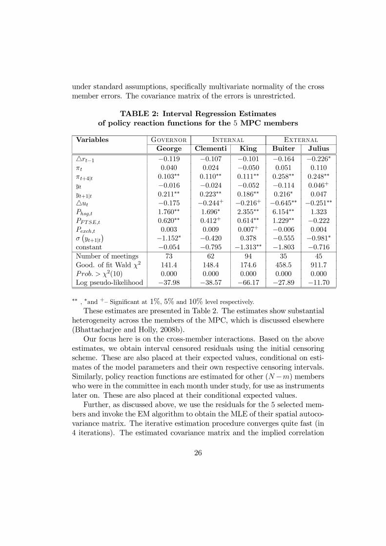
under standard assumptions, speci…cally multivariate normality of the crossmember errors. The covariance matrix of the errors is unrestricted.

TABLE 2: Interval Regression Estimatesof policy reaction functions for the 5 MPC members

Variables Governor Internal ExternalGeorge Clementi King Buiter Julius

4¡1 ¡0119 ¡0107 ¡0101 ¡0164 ¡0226¤

0040 0024 ¡0050 0051 0110+4j 0103¤¤ 0110¤¤ 0111¤¤ 0258¤¤ 0248¤¤

¡0016 ¡0024 ¡0052 ¡0114 0046+

+1j 0211¤¤ 0223¤¤ 0186¤¤ 0216¤ 00474 ¡0175 ¡0244+ ¡0216+ ¡0645¤¤ ¡0251¤¤

1760¤¤ 1696¤ 2355¤¤ 6154¤¤ 1323 0620¤¤ 0412+ 0614¤¤ 1229¤¤ ¡0222 0003 0009 0007+ ¡0006 0004

¡+1j

¢¡1152¤ ¡0420 0378 ¡0555 ¡0981¤

constant ¡0054 ¡0795 ¡1313¤¤ ¡1803 ¡0716

Number of meetings 73 62 94 35 45Good. of …t Wald 2 1414 1484 1746 4585 9117 2(10) 0000 0000 0000 0000 0000Log pseudo-likelihood ¡3798 ¡3857 ¡6617 ¡2789 ¡1170

¤¤ , ¤and +– Signi…cant at 1%, 5% and 10% level respectively.

These estimates are presented in Table 2. The estimates show substantialheterogeneity across the members of the MPC, which is discussed elsewhere(Bhattacharjee and Holly, 2008b).

Our focus here is on the cross-member interactions. Based on the aboveestimates, we obtain interval censored residuals using the initial censoringscheme. These are also placed at their expected values, conditional on esti-mates of the model parameters and their own respective censoring intervals.Similarly, policy reaction functions are estimated for other (¡) memberswho were in the committee in each month under study, for use as instrumentslater on. These are also placed at their conditional expected values.

Further, as discussed above, we use the residuals for the 5 selected mem-bers and invoke the EM algorithm to obtain the MLE of their spatial autoco-variance matrix. The iterative estimation procedure converges quite fast (in4 iterations). The estimated covariance matrix and the implied correlation

26

matrix for the regression errors across the 5 selected members are reportedin Table 3.

The estimated correlation matrix in Table 3 indicate very high correlationcoe¢cients between regression errors corresponding to several pairs of MPCmembers. The CD (cross-section dependence) test (Pesaran, 2004) stronglyrejects the null hypothesis of no cross-section dependence. Estimation of thespatial weights matrix would facilitate understanding of these interactions.

Table 3: Estimated MLEs for Mean Vector, Covariance Matrixand Correlation Matrix of Regression Errors (n = 33 months)14

A. Regression Errors: Mean Vector (MLE)

George Clementi King Buiter Julius00041 ¡00174 ¡00070 00016 ¡00054

B. Regression Errors: Correlation (Covariance) Matrix

George Clementi King Buiter JuliusGeorge 1:00

(000829)

Clementi 09989 1:00(001031)

King 09923 09896 1:00(000871)

Buiter 09573 09679 09558 1:00(000778)

Julius 05184 04934 05182 02965 1:00(000050)

The stage is now set for estimating the matrix of cross member networkinteractions. This is done using the three methodologies described in theprevious section.

First, we estimate the interaction (spatial) weights under suitable struc-tural constraints, using the methodology in Bhattacharjee and Jensen-Butler(2005). Typically, one would then require either ( ¡ 1)2 constraints, orequivalently an appropriate objective function to …x the orthogonal transfor-mation. Bhattacharjee and Jensen-Butler (2005) show that a useful set ofconstraints is symmetry of the spatial weights matrix W . This constraint is,however, not useful in our case since we expect the strength of interactionbetween MPC members often to be asymmetric. For example, it is possiblethat an external member of the MPC arrives at her estimate of the output

14Panel B reports the cross-member correlation matrix, with …gures in parentheses onthe diagonals representing the corresponding variances.

27

gap quite independently of what an internal member does, while the internalmember may position himself strategically after assessing how the externalmember is likely to vote.

We, therefore, build up an alternative set of ( ¡ 1)2 = 10 con-straints. Based on some ideas about the institutional setting of monetarypolicy decision making in the Bank of England, we choose the following setsof restrictions:

1. Row-standardisation: It is quite common in the spatial economet-rics literature to work with a row standardised spatial weights matrix,where the rows sum to unity. This, however, is not strictly relevant inour context because some of the elements in the spatial weights matrixcould be negative. Instead, we standardise rows so that the squaresof the elements in each row sum to unity. This assumption gives us 5constraints.

2. Homoscedasticity: Idiosyncratic error variances (2 ’s) are the samefor George, Clementi and Buiter, and di¤erent and unequal error vari-ances for King and Julius – 2George = 2Clementi = 2Buiter (2 restrictions)

3. Symmetry: Symmetric weights between the internal members and theGovernor –Clementi,King = King,Clementi, George,Clementi = Clementi,George

and George,King = King,George (3 restrictions).

The estimates of the spatial weights and idiosyncratic error variances arepresented in Table 4. As one can see, the restrictions are approximatey satis-…ed. More importantly, con…dence intervals based on the bootstrap indicatethat quite a few of the spatial weights are signi…cant. As discussed ear-lier, non-zero spatial weights in our model are indicative of (a) interactiondue to deliberation and combined decision making within the MPC, and/or (b) strategic interaction. Of particular signi…cance are the negative spa-tial weights. While the process of discussion and agreement to a commonestimate of the output gap would contribute to positive spatial weights, neg-ative weights are almost certainly the outcome of strategic interaction. Inthis context, the negative spatial weights between the Governor and the ex-ternal members (Buiter and Julius) are of particular importance. It wouldappear that the evidence from these estimates point towards possible strate-gic alignment of votes within the MPC.

28

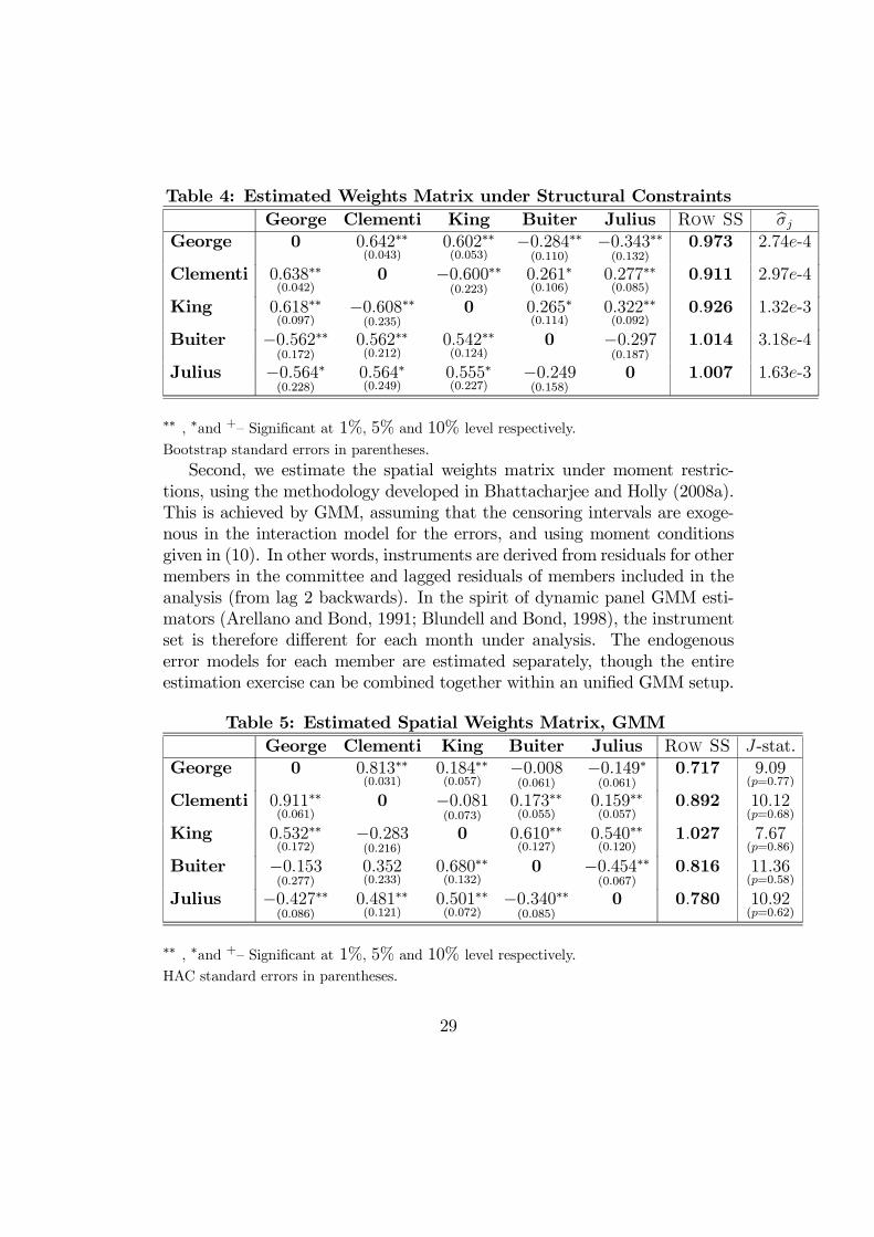
Table 4: Estimated Weights Matrix under Structural Constraints

George Clementi King Buiter Julius Row SS bGeorge 0 0642¤¤

(0043)0602¤¤(0053)

¡0284¤¤(0110)

¡0343¤¤(0132)

0973 274-4

Clementi 0638¤¤(0042)

0 ¡0600¤¤(0223)

0261¤(0106)

0277¤¤(0085)

0911 297-4

King 0618¤¤(0097)

¡0608¤¤(0235)

0 0265¤(0114)

0322¤¤(0092)

0926 132-3

Buiter ¡0562¤¤(0172)

0562¤¤(0212)

0542¤¤(0124)

0 ¡0297(0187)

1014 318-4

Julius ¡0564¤(0228)

0564¤(0249)

0555¤(0227)

¡0249(0158)

0 1007 163-3

¤¤ , ¤and +– Signi…cant at 1%, 5% and 10% level respectively.

Bootstrap standard errors in parentheses.

Second, we estimate the spatial weights matrix under moment restric-tions, using the methodology developed in Bhattacharjee and Holly (2008a).This is achieved by GMM, assuming that the censoring intervals are exoge-nous in the interaction model for the errors, and using moment conditionsgiven in (10). In other words, instruments are derived from residuals for othermembers in the committee and lagged residuals of members included in theanalysis (from lag 2 backwards). In the spirit of dynamic panel GMM esti-mators (Arellano and Bond, 1991; Blundell and Bond, 1998), the instrumentset is therefore di¤erent for each month under analysis. The endogenouserror models for each member are estimated separately, though the entireestimation exercise can be combined together within an uni…ed GMM setup.

Table 5: Estimated Spatial Weights Matrix, GMM

George Clementi King Buiter Julius Row SS -stat.George 0 0813¤¤

(0031)0184¤¤(0057)

¡0008(0061)

¡0149¤(0061)

0717 909(=077)

Clementi 0911¤¤(0061)

0 ¡0081(0073)

0173¤¤(0055)

0159¤¤(0057)

0892 1012(=068)

King 0532¤¤(0172)

¡0283(0216)

0 0610¤¤(0127)

0540¤¤(0120)

1027 767(=086)

Buiter ¡0153(0277)

0352(0233)

0680¤¤(0132)

0 ¡0454¤¤(0067)

0816 1136(=058)

Julius ¡0427¤¤(0086)

0481¤¤(0121)

0501¤¤(0072)

¡0340¤¤(0085)

0 0780 1092(=062)

¤¤ , ¤and +– Signi…cant at 1%, 5% and 10% level respectively.

HAC standard errors in parentheses.

29

The validity of the assumed moment conditions is checked using theSargan-Hansen -test for overidentifying restrictions (Hansen, 1982). Theestimated interaction matrix is presented in Table 5. The reported estimatesare numerically, and de…nitely in sign, similar to estimates of spatial weightsunder structural constraints (Table 4). At the same time, signi…cance ofsome of the weights are di¤erent. Admittedly, the assumed structural re-strictions on the weights matrix are not veri…able and can be violated inempirical applications. This observation further underscores an advantage ofthe GMM based methodology, subject to the validity of the assumed momentconditions. Further, the moment restrictions can be tested, as we have donehere.

Third, we estimate structural spatial weights after allowing for commoncorrelated factors. In the context of the current application, we suspect apriori that the MPC members may not be completely exchangeable. In otherwords, some structural connections may be important. At the same time,unobserved factors may drive some of the cross-section dependence. In orderto explore the relative importance of these two channels, we estimate themodel using the common correlated e¤ects (CCE) methodology (Pesaran,2006). In the current application, none of the variables in the RHS of theempirical policy rule (23) has cross-section variation, but we allow for com-plete slope heterogeneity. Therefore, we estimate a modi…ed policy rule withcross-section averages of the dependent variable as an additional regressor.Very similar results are obtained when we use the median response as a proxyfor this mean response. This also has the advantage of helping place an ex-plicit interpretation to the additional regressor. Decisions of the 9 memberCommittee are made by majority voting so the actual decision which is madeand implemented is the median. We, therefore, report results for the modi…eddecision rule:

= + () 4¡1 +

(0) +

(4) +4j +

(0) j (26)

+(1) +1j +

()

¡+1j

¢+

+

() 4 +

where as before

= W + ;

(0) = § =

¡21

22

2

¢

The covariance and correlation matrix of the residuals from this model isestimated in the same way as before, and reported in Table 6. It is interesting

30

to note that, after allowing for common factors, the degree of structural cross-section dependence has ben reduced signi…cantly, to the extent that the CDtest (Pesaran, 2004) now fails to reject the null hypothesis of no spatialdependence.

Table 6: Estimated MLEs for Mean Vector, Covariance Matrixand Correlation Matrix of Regression Errors in CCE model (26)15

A. Regression Errors: Mean Vector (MLE)

George Clementi King Buiter Julius757-10 ¡00141 ¡00216 ¡00114 00121

B. Regression Errors: Correlation (Covariance) Matrix

George Clementi King Buiter JuliusGeorge 1:00

(000019)

Clementi 01144 1:00(000719)

King ¡00895 01089 1:00(000989)

Buiter ¡02021 00917 03145 1:00(000974)

Julius ¡01117 ¡00140 00440 ¡00435 1:00(001020)

However, some spatial correlations are quite large, and it is possible thata degree of structural spatial interactions may be present. In order to explorethis, we estimate the structural spatial weights matrix by GMM, using thesame moment conditions as before (10). The estimates and correspondingtests for overidentifying restrictions are reported in Table 7.

The estimates point to important structural interconnections betweenmembers of the MPC. Though the statistical signi…cance of spatial interac-tions is weaker than those reported before (Tables 4 and 5), the direction andmagnitude of the important network e¤ects are broadly preserved. Furtheranalysis of network connections within the Bank of England’s MPC, and re-lated inferences on network architecture and strategic behaviour, is beyondthe scope of this paper.

Therefore, overall we can conclude that the objective of studying spatialinteractions is best served by allowing for both structural and factor based

15Panel B reports the cross-member correlation matrix, with …gures in parentheses onthe diagonals representing the corresponding variances.

31

cross-section dependence. Further, we describe and illustrate several methodsbased on spatial panel data that can be used to draw inferences on thesespatial and interaction weights.

Table 7: Estimated Spatial Weights Matrix by GMM(allowing for common unobserved factors – CCE)

George Clementi King Buiter Julius -stat.George 0 00015

(00087)¡00096(00099)

¡00060(00121)

¡00279¤(00134)

877(=079)

Clementi ¡04976(05561)

0 01516(01055)

02511+(01365)

¡01458(01389)

846(=081)

King 02936(14663)

02393+(01431)

0 03319¤(01467)

04021¤(01769)

875(=079)

Buiter 22354+(13537)

00326(00994)

06435¤¤(01198)

0 ¡00234(01251)

1078(=063)

Julius ¡26098¤¤(09904)

00105(01136)

¡00231(01078)

01583(01198)

0 873(=079)

¤¤ , ¤and +– Signi…cant at 1%, 5% and 10% level respectively.

HAC standard errors in parentheses.

4 Conclusions

In this paper, we argue that the distinction between structural and factorbased connections is very important in the study of spatial and cross-sectioninteractions. Both of these channels o¤er alternative explanations for spa-tial correlation and can coexist in some models and applications. Further,while the assumption of exchangebility inherent in the factor model can beunreasonable in many spatial applications, assuming the absence of commonunobserved factors also appears to be too strong.

We describe three methods to draw inferences on spatial (interaction)weights that explicitly address the above distinction. The …rst two methodsare designed to draw inferences under the structural dependence assump-tion, one under structural constraints on the spatial weights matrix (Bhat-tacharjee and Jen-Butler, 2005) and the other under moment restrictions in-spired by the system GMM literature (Bhattacharjee and Holly, 2008a). Thethird method allows for both structural and factor based dependence, wherethe unobserved factors are modelled using the common correlated e¤ectsmethodology (Pesaran, 2006) and the structural spatial weights estimatedusing GMM methods propoesed in Bhattacharjee and Holly (2008a). The

32

methods are illustrated using an application to committee decision makingwithin the Bank of England’s MPC. The application highlights the relativeadvantages and shortcomings of each of the methods, and helps draw usefulinferences on the nature and strength of interactions.

Research in the above area, both empirical and econometric, is ongo-ing. More work needs to be done in combining the common factor approachwith structural spatial interactions. Further research on the nature of spatialinteractions would inform both the very active theoretical literature on eco-nomic networks, and provide additional empirical insights into the stabilityof di¤erent network architectures under assumptions on information sharingand bargaining. Also, the networks emerging from our work can be viewedas a sequence of weighted directed graphs, with connections condituioned onthe assumed signi…cance level. How research on such random graphs canaid inferences on connections in space and economic networks is a matter offurther study.

Apart from the application developed here, Bhattacharjee and Jensen-Butler (2005) and Holly et al. (2006) have used related frameworks for em-pirical studies of housing markets. However, the applicability of the frame-work and methods would surely go beyond these couple of applications. Forexample, an important application area would be economic convergence ofcountries and regions; see Bhattacharjee and Jensen-Butler (2005) for a simu-lation study based on the US. Previous research suggests that there are stabledi¤erences in productivity across regions in the EU. Potentially, such spa-tial inequality can be explained by technology transfer, where some regionsare more e¢cient in generating new technology or technology absorption. Inturn, technology transfer is often related to trade, FDI etc., while technologyabsorption depends on human capital, R&D and similar features. However,theory provides no clear guidance as to which of these channels are moreimportant, or indeed if relative importance varies across regions. Further,while some of the di¤usion can be explained by the pull of common factors,there may be institutional features that enhance or depress technology trans-fer between speci…c pairs of regions. In empirical studies, it is useful to allowfor technology transfer in relatively unrestricted manner and further, to inferon the strength and direction of inter-region di¤usion while being agnosticabout the speci…c drivers of such interaction. Further research along sim-ilar lines will be important for our understanding of economic growth andconvergence.

33

References

[1] Amemiya, T. (1973). Regression analysis when the dependent variableis truncated normal. Econometrica 41, 997–1016.

[2] Andrews, D.W.K. (2005). Cross-section regression with common shocks.Econometrica 73, 1551–1585.

[3] Anselin, L. (1988). Spatial Econometrics: Methods and Models. KluwerAcademic Publishers: Dordrecht, The Netherlands.

[4] Anselin, L. (1999). Spatial econometrics. In Baltagi, B.H. (Ed.), A Com-panion to Theoretical Econometrics. Oxford: Basil Blackwell, 310–330.

[5] Anselin, L. (2002). Under the hood: Issues in the speci…cation and in-terpretation of spatial regression models. Agricultural Economics 27,247–267.

[6] Anselin, L., Florax, R. and Rey, S. (2003). Econometrics for spatialmodels: recent advances. In Anselin, L., Florax, R. and Rey, S. (Eds.)Advances in Spatial Econometrics. Springer-Verlag: Berlin.

[7] Aoki, K. (2003). On the optimal monetary policy response to noisyindicators. Journal of Monetary Economics 50, 501–523.

[8] Arellano, M. and Bond, S. (1991). Some tests of speci…cation for paneldata: Monte Carlo evidence and an application to employment equa-tions. Review of Economic Studies 58, 277–297.

[9] Austen-Smith, D. and Banks, J.S. (1996). Information aggregation, ra-tionality, and the Condorcet jury theorem. American Political ScienceReview 90, 34–45.

[10] Bai, J. (2009). Likelihood approach to small T dynamic panel data mod-els with interactive e¤ects. Paper presented at an Invited Session in the15 International Panel Data Conference, Bonn, 2009. Mimeo.

[11] Baltagi, B.H., Egger, P. and Pfa¤ermayr, M. (2006). A generalized spa-tial panel data model with random e¤ects. Working paper, SyracuseUniversity, Department of Economics and Center for Policy Research.

34

[12] Baltagi, B.H., Egger, P. and Pfa¤ermayr, M. (2007). A monte carlostudy for pure and pretest estimators of a panel data model with spa-tially autocorrelated disturbances. Annales d’Economie et de Statistique(forthcoming).

[13] Bhattacharjee, A. and Holly, S. (2008a). Understanding interactions insocial networks and committees. Mimeo.

[14] Bhattacharjee, A. and Holly, S. (2008b). Taking personalities out ofmonetary policy decision making? interactions, heterogeneity and com-mittee decisions in the Bank of England’s MPC. Mimeo. Previous versionavailable as: CDMA Working Paper 0612 (2006), Centre for DynamicMacroeconomic Analysis, University of St. Andrews, UK..

[15] Bhattacharjee, A. and Jensen-Butler, C. (2005). Estimation of spatialweights matrix in a spatial error model, with an application to di¤usionin housing demand. CRIEFF Discussion Paper No. 0519, University ofSt. Andrews, UK.

[16] Blundell, R. and Bond, S. (1998). Initial conditions and moment re-strictions in dynamic panel data models. Journal of Econometrics 87,115–143.

[17] Blundell, R.W. and Smith, R. (1986) An exogeneity test for the si-multaneous equation tobit model with an application to labor supply.Econometrica 54, 679–685.

[18] Britton, E., Fisher, P.G. and Whitley, J.D. (1998). The in‡ation reportprojections: understanding the fan chart. Bank of England QuarterlyBulletin 38, 30–37.

[19] Coakley, J., Fuertes, A.M., and Smith, R. (2002). A principal compo-nents approach to cross-section dependence in panels. Birkbeck CollegeDiscussion Paper 01/2002.

[20] Conley, T.G. (1999). GMM estimation with cross sectional dependence.Journal of Econometrics 92, 1–45.

[21] Conley, T.G. and Molinari, F. (2007). Spatial correlation robust infer-ence with errors in location or distance. Journal of Econometrics 140,76–96.

35

[22] Conley, T.G. and Topa, G. (2002). Socio-economic distance and spatialpatterns in unemployment. Journal of Applied Econometrics 17, 303–327.

[23] Conley, T.G. and Topa, G. (2003). Identi…cation of local interactionmodels with imperfect location data. Journal of Applied Econometrics18, 605–618.

[24] de Finetti, B. (1937). La prévision: ses lois logiques, ses resources sub-jectives. Annales de l 0Institut Henri Poincaré 7, 1–68. English transla-tion: Foresight: its logical laws, its subjective sources, in Kyburg, H.E.and Smokler, H.E. (Eds.), Studies in Subjective Probability, New York:Wiley, 1964.

[25] Dempster, A., Laird, N. and Rubin, D. (1977). Maximum likelihood forincomplete data via the EM algorithm. Journal of the Royal StatisticalSociety Series B 39, 1–38.

[26] Dubin, R.A. (2009). Spatial Weights. In Fotheringham, A.S. and Roger-son, P.A. (Eds.), The SAGE Handbook of Spatial Analysis. London: SagePublications, 125–158.

[27] Dutta, B. and Jackson, M.O. (2003). Networks and Groups: Models ofStrategic Formation. Springer Verlag: Berlin.

[28] Evans, P. and Karras, G. (1996). Convergence revisited. Journal of Mon-etary Economics 37, 249–265.

[29] Fingleton, B. (2003). Externalities, economic geography and spatialeconometrics: conceptual and modeling developments. International Re-gional Science Review 26, 197–207.

[30] Fingleton, B. (2008). A generalized method of moments estimator for aspatial model with moving average errors, with application to real estateprices. Empirical Economics 34, 35–57.

[31] Forni, M., Hallin, M., Lippi, M. and Reichlin, L. (2004). The generalizeddynamic factor model consistency and rates. Journal of Econometrics119, 231–255.

36

[32] Gerlach-Kristen, P. (2004). Is the MPC’s voting record informativeabout future UK monetary policy?. Scandinavian Journal of Economics106 (2), 299–314.

[33] Giacomini, R., Granger, C.W.J. (2004) Aggregation of space-timeprocesses, Journal of Econometrics, 118, 7-26

[34] Gibbons, S and Machin, S. (2005). Valuing rail access using transportinnovations. Journal of Urban Economics 57, 148–169.

[35] Goyal, S. (2005). Strong and weak links. Journal of the European Eco-nomic Association 3, 608–616.

[36] Goyal, S. (2007). Connections: an Introduction to the Economics ofNetworks. Princeton University Press.

[37] Granovetter, M.S. (1973). The strength of weak ties. American Journalof Sociology 78, 1360–1380.

[38] Gulliksen, H. (1968). Methods for determining equivalence of measures.Psychological Bulletin 70, 534–544.

[39] Hansen, L. (1982). Large sample properties of generalized method ofmoments estimators. Econometrica 50, 1029–1054.

[40] Hewitt, E. and Savage, L. (1955). Symmetric measures on cartesianproducts. Transaction of the American Mathematical Society 80, 470–501.

[41] Holly, A., Pesaran, M.H. and Yamagata, T. (2006). A spatio-temporalmodel of house prices in the US. Cambridge Working Papers in Eco-nomics 0654, University of Cambridge. Journal of Econometrics (forth-coming).

[42] Issing, O. (2002). Monetary policy in a world of uncertainty. Presentedat the Economic Policy Forum, Banque de France, Paris, 9 Dec. 2002.

[43] Jennrich, R.I. (2001). A simple general procedure for orthogonal rota-tion. Psychometrika 66, 289–306.

37

[44] Kapoor, M., Kelejian, H.H., and Prucha, I.R. (2007). Panel data mod-els with spatially correlated error components. Journal of Econometrics140, 97–130.

[45] Kelderman, H. (2004). Measurement exchangeability and normal one-factor models. Biometrika 91, 738–742.

[46] Kelejian, H.H. and Prucha, I.R. (1999). A generalized moments estima-tor for the autoregressive parameter in a spatial models. InternationalEconomic Review 40, 509–533.

[47] Kelejian, H.H. and Prucha, I.R. (2004). Estimation of simultaneoussystems of spatially interrelated cross sectional equations. Journal ofEconometrics 118, 27–50.

[48] Kelejian, H.H. and Prucha, I.R. (2007). HAC estimation in a spatialframework. Journal of Econometrics 140, 131–154.

[49] King, M. (2002). The Monetary Policy Committee …ve years on. Addressto the Society of Business Economists, London, 22 May 2002 (availablefrom http://www.bankofengland.co.uk/speeches/speaker.htm).

[50] Newey, W.K. (1984). A method of moments interpretation of sequentialestimators. Economics Letters 14, 201–206.

[51] Orphanides, A. (2003). Monetary policy evaluation with noisy informa-tion. Journal of Monetary Economics 50, 605–631.

[52] Pesaran, M.H. (2004). General diagnostic tests for cross section depen-dence in panels. CESifo Working Papers, No. 1233.

[53] Pesaran, M.H. (2006). Estimation and inference in large heterogenouspanels with multifactor error structure. Econometrica 74, 967–1012.

[54] Pesaran, M.H., Schuermann, T. and Weiner, S. (2004). Modelling re-gional interdependencies using a global error-correcting macroeconomet-ric model. Journal of Business and Economics Statistics 22, 129–162.

[55] Pesaran, M.H. and Tosetti, E. (2007). Large panels with common fac-tors and spatial correlations.Working Paper CWPE 0743, Faculty ofEconomics, University of Cambridge.

38

[56] Pinkse, J., Slade, M.E. and Brett, C. (2002). Spatial price competition:a semiparametric approach. Econometrica 70, 1111–1155.

[57] Svensson, L. (1997). In‡ation forecast targeting: implementing and mon-itoring in‡ation targets. European Economic Review 41, 1111–1146.

39

www.st-and.ac.uk/cdma

ABOUT THE CDMA

The Centre for Dynamic Macroeconomic Analysis was established by a direct grant from theUniversity of St Andrews in 2003. The Centre funds PhD students and facilitates a programme ofresearch centred on macroeconomic theory and policy. The Centre has research interests in areas such as:characterising the key stylised facts of the business cycle; constructing theoretical models that can matchthese business cycles; using theoretical models to understand the normative and positive aspects of themacroeconomic policymakers' stabilisation problem, in both open and closed economies; understandingthe conduct of monetary/macroeconomic policy in the UK and other countries; analyzing the impact ofglobalization and policy reform on the macroeconomy; and analyzing the impact of financial factors onthe long-run growth of the UK economy, from both an historical and a theoretical perspective. TheCentre also has interests in developing numerical techniques for analyzing dynamic stochastic generalequilibrium models. Its affiliated members are Faculty members at St Andrews and elsewhere withinterests in the broad area of dynamic macroeconomics. Its international Advisory Board comprises agroup of leading macroeconomists and, ex officio, the University's Principal.

Affiliated Members of the School

Dr Fabio Aricò.Dr Arnab Bhattacharjee.Dr Tatiana Damjanovic.Dr Vladislav Damjanovic.Prof George Evans.Dr Gonzalo Forgue-Puccio.Dr. Michal HorvathDr Laurence Lasselle.Dr Peter Macmillan.Prof Rod McCrorie.Prof Kaushik Mitra.Dr. Elisa NewbyProf Charles Nolan (Director).Dr Geetha Selvaretnam.Dr Ozge Senay.Dr Gary Shea.Prof Alan Sutherland.Dr Kannika Thampanishvong.Dr Christoph Thoenissen.Dr Alex Trew.

Senior Research Fellow

Prof Andrew Hughes Hallett, Professor of Economics,Vanderbilt University.

Research Affiliates

Prof Keith Blackburn, Manchester University.Prof David Cobham, Heriot-Watt University.Dr Luisa Corrado, Università degli Studi di Roma.Prof Huw Dixon, Cardiff University.Dr Anthony Garratt, Birkbeck College London.Dr Sugata Ghosh, Brunel University.Dr Aditya Goenka, Essex University.Dr Michal Horvath, University of Oxford.Prof Campbell Leith, Glasgow University.Prof Paul Levine, University of Surrey.Dr Richard Mash, New College, Oxford.Prof Patrick Minford, Cardiff Business School.Dr Elisa Newby, University of Cambridge.

Dr Gulcin Ozkan, York University.Prof Joe Pearlman, London Metropolitan University.Prof Neil Rankin, Warwick University.Prof Lucio Sarno, Warwick University.Prof Eric Schaling, South African Reserve Bank and

Tilburg University.Prof Peter N. Smith, York University.Dr Frank Smets, European Central Bank.Prof Robert Sollis, Newcastle University.Prof Peter Tinsley, Birkbeck College, London.Dr Mark Weder, University of Adelaide.

Research Associates

Mr Nikola Bokan.Mr Farid Boumediene.Miss Jinyu Chen.Mr Johannes Geissler.Mr Ansgar Rannenberg.Mr Qi Sun.

Advisory Board

Prof Sumru Altug, Koç University.Prof V V Chari, Minnesota University.Prof John Driffill, Birkbeck College London.Dr Sean Holly, Director of the Department of Applied

Economics, Cambridge University.Prof Seppo Honkapohja, Bank of Finland and

Cambridge University.Dr Brian Lang, Principal of St Andrews University.Prof Anton Muscatelli, Heriot-Watt University.Prof Charles Nolan, St Andrews University.Prof Peter Sinclair, Birmingham University and Bank of

England.Prof Stephen J Turnovsky, Washington University.Dr Martin Weale, CBE, Director of the National

Institute of Economic and Social Research.Prof Michael Wickens, York University.Prof Simon Wren-Lewis, Oxford University.

www.st-and.ac.uk/cdmaRECENT WORKING PAPERS FROM THE

CENTRE FOR DYNAMIC MACROECONOMIC ANALYSIS

Number Title Author(s)

CDMA07/21 Unconditionally Optimal MonetaryPolicy

Tatiana Damjanovic (St Andrews),Vladislav Damjanovic (St Andrews)and Charles Nolan (St Andrews)

CDMA07/22 Estimating DSGE Models under PartialInformation

Paul Levine (Surrey), JosephPearlman (London Metropolitan) andGeorge Perendia (LondonMetropolitan)

CDMA08/01 Simple Monetary-Fiscal Targeting Rules Michal Horvath (St Andrews)

CDMA08/02 Expectations, Learning and MonetaryPolicy: An Overview of Recent Research

George Evans (Oregon and StAndrews), Seppo Honkapohja (Bankof Finland and Cambridge)

CDMA08/03 Exchange rate dynamics, asset marketstructure and the role of the tradeelasticity

Christoph Thoenissen (St Andrews)

CDMA08/04 Linear-Quadratic Approximation toUnconditionally Optimal Policy: TheDistorted Steady-State

Tatiana Damjanovic (St Andrews),Vladislav Damjanovic (St Andrews)and Charles Nolan (St Andrews)

CDMA08/05 Does Government Spending OptimallyCrowd in Private Consumption?

Michal Horvath (St Andrews)

CDMA08/06 Long-Term Growth and Short-TermVolatility: The Labour Market Nexus

Barbara Annicchiarico (Rome), LuisaCorrado (Cambridge and Rome) andAlessandra Pelloni (Rome)

CDMA08/07 Seigniorage-maximizing inflation Tatiana Damjanovic (St Andrews)and Charles Nolan (St Andrews)

CDMA08/08 Productivity, Preferences and UIPdeviations in an Open EconomyBusiness Cycle Model

Arnab Bhattacharjee (St Andrews),Jagjit S. Chadha (Canterbury) and QiSun (St Andrews)

CDMA08/09 Infrastructure Finance and IndustrialTakeoff in the United Kingdom

Alex Trew (St Andrews)

CDMA08/10 Financial Shocks and the US BusinessCycle

Charles Nolan (St Andrews) andChristoph Thoenissen (St Andrews)

CDMA09/01 Technological Change and the RoaringTwenties: A Neoclassical Perspective

Sharon Harrison (Columbia) MarkWeder (Adeleide)

www.st-and.ac.uk/cdmaCDMA09/02 A Model of Near-Rational Exuberance George Evans (Oregon and St

Andrews), Seppo Honkapohja (Bankof Finland and Cambridge) andJames Bullard (St Louis Fed)

CDMA09/03 Shocks, Monetary Policy andInstitutions: Explaining UnemploymentPersistence in “Europe” and the UnitedStates

Ansgar Rannenberg (St Andrews)

CDMA09/04 Contracting Institutions and Growth Alex Trew (St Andrews)

CDMA09/05 International Business Cycles and theRelative Price of Investment Goods

Parantap Basu (Durham) andChristoph Thoenissen (St Andrews)

CDMA09/06 Institutions and the Scale Effect Alex Trew (St Andrews)

CDMA09/07 Second Order Accurate Approximationto the Rotemberg Model Around aDistorted Steady State

Tatiana Damjanovic (St Andrews)and Charles Nolan (St Andrews)

CDMA09/08 Both Sides of the Story: Skill-biasedTechnological Change, Labour MarketFrictions, and Endogenous Two-SidedHeterogeneity

Fabio R. Aricó (St Andrews)

CDMA09/09 The Taylor Principle and (In-)Determinacy in a New Keynesian Modelwith hiring Frictions and Skill Loss

Ansgar Rannenberg (St Andrews)

CDMA10/01 Sunspots and Credit Frictions Sharon Harrison (Columbia) andMark Weder (Adelaide, CDMA andCEPR)

CDMA10/02 Endogenous Persistence in an EstimatedDSGE Model under ImperfectInformation

Paul Levine (Surrey), JosephPearlman (London Metropolitan),George Perendia (LondonMetropolitan) and Bo Yang (Surrey)

..

For information or copies of working papers in this series, or to subscribe to email notification, contact:

Jinyu ChenCastlecliffe, School of Economics and FinanceUniversity of St AndrewsFife, UK, KY16 9ALEmail: jc736@at-andrews.ac.uk; Phone: +44 (0)1334 462445; Fax: +44 (0)1334 462444.