processes help build a quantitative literacy that can betransferred and applied to the other processes.

A SIPHON EXPERIMENTMy most-used decay experiments involve flowing

water, and can be done with a "V-tube" or a siphon.Geologists think a lot about flowing water. Streams,erosion, groundwater, and flooding are topics inintroductory and advanced geology courses, and some ofthe principles of flowing water are familiar to evenbeginning students. I find that most geology students areable to make good predictions when presented with theexperimental design shown in Figure 1. The "V-tube"apparatus consists of two vertical plastic tubes (44.5 mmi.d.) connected at their bases by a copper pipe (12.7 mm

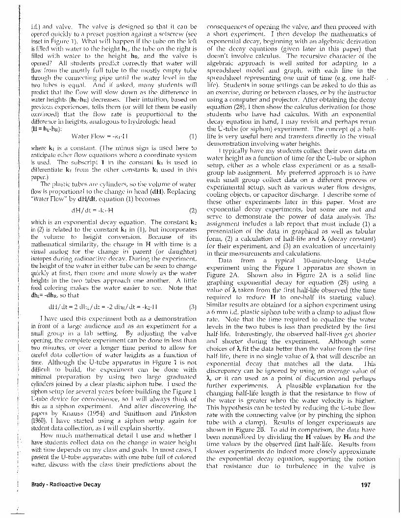
FIGVRE 1. A schematicdrawing of a "V-tube"apparatus, consisting oftwo vertical plastic tubesconnected by a horizon­tal tube with a valve. Thetube at the left is filledwith water to height hL;the tube at the right isfilled with water to theheight hn. If the valve isopened, water will flowfrom the tube on the leftto the tube on the right ata rate that is proportionalto the difference inheights H. The insetphoto is a close-up viewof the valve and setscrewmechanism to presetthree valve positionsand, therefore, flowrates.

Journal of Geoscience Education, v. 57, n. 3, May, 2009, p. 196-205196

ABSTRACTAlthough an understanding of radiometric dating is central to the preparation of every geologist, many studentsstruggle with the concepts and mathematics of radioactive decay. Physical demonstrations and hands-on experimentscan be used to good effect in addressing this teaching conundrum. Water, heat, and electrons all move or flow inresponse to generalized forces (gradients in pressure, temperature, and electrical potential) that may change because ofthe flow. Changes due to these flows are easy to monitor over time during simple experiments in the classroom. Someof these experiments can be modeled as exponential decay, analogous to the mathematics of radioactive decay, and canbe used to help students visualize and understand exponential change. Other, similar experiments produce decay orchange that is not exponential. By having classes, in small groups, conduct several experiments involving flows, alearning synergy can be encouraged in which the physical and mathematical similarities of flow processes areemphasized. For the best results, students should be asked to analyze the experimental data, using graphs and algebraor calculus as appropriate to the class, to determine the nature of the decay process and to make predictions, eitherforward or backward in time as would be done for radiometric dating. Basic quantitative skills are strengthened ordeveloped as part of these activities. Encountering a number of important geologic processes in the same mathematical

Siphons. Water Clocks, Cooling Coffee, and Leaking Capacitors:Classroom Activities and a few Equations to Help StudentsUnderstand Radioactive Decay and Other Exponential ProcessesJohn B. Brady 1

'Department of Geology, Smith College, Northampton, MA 01063;jbrady@smith.edu

INTRODUCTIONRadiometric dating provides essential data for much

of our geologic understanding of earth history and,therefore, is an important topic for many courses ingeology. Because calculus is typically used in developingthe mathematics of radioactive decay, students withoutcalculus are likely to have difficulty in grasping some ofthe principles of radiometric dating and in applying therelevant equations. The significance of radioactivity,exponential decay, and radiometric dating to geologists,chemists, and physicists and the challenges of teachingabout these topics have led to numerous publishedpedagogic strategies. These include stochastic experimentswith coins (Kowalski, 1981; Tyburczy, 2000; Wenner,2008a), dice (Celnikier, 1980; Priest and Poth, 1983;Schultz, 1997; Benimoff, 1999), poker chips (McGeachy,1988), M&M's (AAAS Science Netlinks, 2001a; Gardner etal., 2005; Wenner, 2008b), or popcorn (Wenner, 2008c),measurements of actual radioactive decay (Jones, 1957;Whyte and Taylor, 1962; Supan and Kraushaar, 1983),analog experiments (Bohn and Nadig, 1938; Knauss, 1954;Smithson and Pinkston, 1960; Wunderlich and Peastrel,1978; Wise, 1990; AAAS Science Netlinks, 2001b;Greenslade, 2002; Fairman et al., 2003; Sunderman, 2007),and general mathematical approaches or advice(Guenther, 1958; Vacher, 2000; Shea, 2001; Huestis, 2002).I have tried a number of classroom activities to helpstudents understand the mathematics of radioactivedecay, and describe here some of the more successfulexperiments that I find useful for geology classes. Ibelieve that having classes do several of the experiments,simultaneously in small groups, demonstrates themathematical connectedness of a variety of importantgeologic processes. Furthermore, the data collection andanalysis skills learned by studying anyone of the

where k j is a constant. (The minus sign is used here toanticipate other flow equations where a coordinate systemis used. The subscript 1 in the constant ki is used todifferentiate k 1 from the other constants k, used in thispaper.)

The plastic tubes are cylinders, so the volume of waterflow is proportional to the change in head (dH). Replacing"Water Flow" by dHjdt, equation (1) becomes

dH/ dt = -k-H (2)

which is an exponential decay equation. The constant k 2

in (2) is related to the constant k1 in (1), but incorporatesthe volume to height conversion. Because of itsmathematical similarity, the change in H with time is avisual analog for the change in parent (or daughter)isotopes during radioactive decay. During the experiment,the height of the water in either tube can be seen to changequickly at first, then more and more slowly as the waterheights in the two tubes approach one another. A littlefood coloring makes the water easier to see. Note thatdh,=-dh R, so that

i.d.) and valve. The valve is designed so that it can beopened quickly to a preset position against a setscrew (seeinset in Figure 1). What will happen if the tube on the leftisfilled with water to the height h L, the tube on the right isfilled with water to the height hR, and the valve isopened? All students predict correctly that water willflow from the mostly full tube to the mostly empty tubethrough the connecting pipe until the water level in thetwo tubes is equal. And if asked, many students willpredict that the flow will slow down as the difference inwater heights (hL-hR) decreases. Their intuition, based onprevious experiences, tells them (or will let them be easilyconvinced) that the flow rate is proportional to thedifference in heights, analogous to hydrologic head(H= hi-hn]:

I have used this experiment both as a demonstrationin front of a large audience and as an experiment for asmall group in a lab setting. By adjusting the valveopening, the complete experiment can be done in less thantwo minutes, or over a longer time period to allow forcareful data collection of water heights as a function oftime. Although the U-tube apparatus in Figure 1 is notdifficult to build, the experiment can be done withminimal preparation by using two large graduatedcylinders joined by a clear plastic siphon tube. I used thesiphon setup for several years before building the Figure 1U-tube device for convenience, so I will always think ofthis as a siphon experiment. And after discovering thepapers by Knauss (1954) and Smithson and Pinkston(1960), I have started using a siphon setup again forstudent data collection, as I will explain shortly.

How much mathematical detail I use and whether Ihave students collect data on the change in water heightwith time depends on my class and goals. In most cases, Ipresent the U-tube apparatus with one tube full of coloredwater, discuss with the class their predictions about the

consequences of opening the valve, and then proceed witha short experiment. I then develop the mathematics ofexponential decay, beginning with an algebraic derivationof the decay equations (given later in this paper) thatdoesn't involve calculus. The recursive character of thealgebraic approach is well suited for adapting to aspreadsheet model and graph, with each line in thespreadsheet representing one unit of time (e.g. one half­life). Students in some settings can be asked to do this asan exercise, during or between classes, or by the instructorusing a computer and projector. After obtaining the decayequation (28), I then show the calculus derivation for thosestudents who have had calculus. With an exponentialdecay equation in hand, I may revisit and perhaps rerunthe U-tube (or siphon) experiment. The concept of a half­life is very useful here and transfers directly to the visualdemonstration involving water heights.

I typically have my students collect their own data onwater height as a function of time for the U-tube or siphonsetup, either as a whole class experiment or as a small­group lab assignment. My preferred approach is to haveeach small group collect data on a different process orexperimental setup, such as various water flow designs,cooling objects, or capacitor discharge. I describe some ofthese other experiments later in this paper. Most areexponential decay experiments, but some are not andserve to demonstrate the power of data analysis. Theassignment includes a lab report that must include (1) apresentation of the data in graphical as well as tabularform, (2) a calculation of half-life and A (decay constant)for their experiment, and (3) an evaluation of uncertaintyin their measurements and calculations.

Data from a typical 10-minute-long U-tubeexperiment using the Figure 1 apparatus are shown inFigure 2A. Shown also in Figure 2A is a solid linegraphing exponential decay for equation (28) using avalue of A taken from the first half-life observed (the timerequired to reduce H to one-half its starting value).Similar results are obtained for a siphon experiment usinga 6 mm i.d. plastic siphon tube with a clamp to adjust flowrate. Note that the time required to equalize the waterlevels in the two tubes is less than predicted by the firsthalf-life. Interestingly, the observed half-lives get shorterand shorter during the experiment. Although somechoices of A fit the data better than the value from the firsthalf-life, there is no single value of A that will describe anexponential decay that matches all the data. Thisdiscrepancy can be ignored by using an average value ofA, or it can used as a point of discussion and perhapsfurther experiments. A plausible explanation for thechanging half-life length is that the resistance to flow ofthe water is greater when the water velocity is higher.This hypothesis can be tested by reducing the U-tube flowrate with the connecting valve (or by pinching the siphontube with a clamp). Results of longer experiments areshown in Figure 2B. To aid in comparison, the data havebeen normalized by dividing the H values by Ho and thetime values by the observed first half-life. Results fromslower experiments do indeed more closely approximatethe exponential decay equation, supporting the notionthat resistance due to turbulence in the valve is

(1)

(3)

Water Flow = -k.H

dH/ dt = 2 dh L / dt = -2 dhr) dt = -kr-H

Brady- Radioactive Decay 197

80 responsible for the observed decrease in half-life as Hdecreases.

Smithson and Pinkston (1960), following Knauss(1954), present a hydrodynamic design that yields goodexponential decay data using a tall vertical tube and a 1.25-meter-long capillary tube drain, making the flow slowenough to be viscosity-controlled and follow Poiseuille'sLaw (see also Skinner, 1971). Their resu Its encouraged meto try a 1.25-meter-long capillary-sized (2 mrn i.d.) plasticsiphon tube, instead of the larger (6 mm i.d.) tubing I hadbeen using. Data from a siphon experiment with the 2mm i.d. siphon are shown on a semi-log graph in Figure2C along with some of the Ll-tube data of Figure 2B. If In(H/Ho) is plotted vs. time t, exponential decay data shouldfall along a straight line with slope - A (see equation 27).The siphon data fall nicely along the exponential decayline in Figure 2C showing the advantage of the smalltubing size and absence of a constriction. A drawback isthe length of the experiment, but this can be mitigated byusing smaller i.d. vertical tubes or by collecting only partof the data, which would still permit an evaluation of A..Because of the variability of the siphon start, results arebetter if you get the siphon flowing before recording thestarting value of H (=Ho) for your data set.

A related experimental option also may be available ifsomeone in your department studies groundvvater. Acommon tool for laboratorv measurement of hvdraulicconductivity is a perrneameter. which may be used in aconstant-head in or a falling-head geometry (Fetter, 2001).A falling-head experiment is similar to the Smithson andPinkston (1960) experiment, but with a soil samplereplacing the capillary tube in the role of slowing the flowand keeping it in the lamellar flow regime. Some effortand experimentation is needed to find a soil sample thathas a low enough permeability to allow precisemeasurement of head height as a function of time.

600

2mm Siphon

180 Minute U-tube

10 Minute U-tube

Exponential Decay

•••• 10 Minute U-tube

-~- Exponential Decay

400 Minute U-tube

130 Minute u-tubc

10 Minute U-tube

-- Exponential Decay

oo

3 4

t (half-lives)

3 4

t (half-lives)

'.'.'.'.'...... ......200 300 400 500

t (seconds)100

B.

c.

A.oL--------'-----'-__-'--_~~~__..____J

o

-5 L-_-,__~__-,---,--_~__-,-=-----,o

20

0.0 L_--'-__-'--_~~~~2;;c:;WJ::=~o

-4

-1

~-2

~<:.... -3

0.6o

J:

J: 0.4

0.2

Vi~ 60OJ

.~~ 40~

J:

FIGURE 2. Data from U-tube and siphon experiments.(A) Data from a 10-minute-long U-tube experiment areshown in terms of the height difference H and time t.Ideal exponential decay is shown as a solid curve usingthe experimental time for H to fall to half its startingvalue (144 seconds for this experiment) to define the half­life length. Note that the second and subsequent half­lives of the siphon experiment are shorter than the firsthalf-life. (B) Data from three U-tube experiments areshown in terms of the fraction H/Ho of the original heightdifference Ho and time t given as "half-lives", using theexperimental time for H/Ho to fall to 0.5 to define the half-life length for each experiment. Ideal exponential decayis shown as a solid curve. Longer siphon experimentswith slower flow rates more nearly approximate idealexponential decay. (C) Data from a siphon experimentusing a 2 mm i.d. siphon are shown in terms of the natu­ral log of the fraction H/Ho of the original height differ­ence Ho and time t given as "half-lives", using the firstexperimental half-life to normalize the data. Ideal expo­nential decay is shown as a solid straight line. Alsoshown for comparison are U-tube experimental data from(A). The siphon data follow an exponential decay trendvery closely when a "capillary-sized" siphon is used.

1.0

A. C. ,,,

c:::=J,

0.6

s:.t:

/' D.:

0.00 ,

t (half-lives)

FIGURE 3. Drawings of water clock designs discussed inthe text. (A) A cylinder with a hole near the bottom. (B) Acone with a hole at the bottom and water draining into acylindrical collection vessel. (C) A bucket-shaped waterclock with a bottom that is one-half the diameter of thetop. (D) Height of the water h in a cylindrical tank that isleaking from a hole near the bottom (A) shown as a func­tion of time t. The height h is given as a fraction hjho ofthe starting height hn and the time t is given in units ofhalf-lives, using the time for the water level to fall to one­half the original height to define the half-life. Ideal expo­nential decay is shown as a dashed curve. Neither theleaking tank nor exponential decay exhibits linear varia­tion of water height with time, especially after the firsthalf-life.

198 Journal of Geoscience Education, v. 57, n. 3, May, 2009, p. 196-205

(6)

(5)

(9)

(7)

(8)

h

IT 2 'V = -(tan <jJ) h'3

( dh I = ( -k\) fh = (-k.)) fhldt) T(·r-

Integration of (5) yields an expression for the water levelin the cylindrical tank as a function of time:

Differentiating (7 with respect to h and using (4) we find:

[dh '. [dh YdV I = (-k 3).,fh ')dt) dv)l dt ) TC (talnp)h~

Solving (8) for a cone-shaped, dripping water clockwith an initial water depth of one (h=l for t=O) gives theexpression for the water height h as a function of time t:

[ )) ' ;

h = 1 _ 5 k 3 t - ,

2 TC (tan 2 <jJ)

assuming that h=l at t=O. The interested reader can verifythis result by differentiating (6) with respect to t andcomparing the result with (5), using (6) to get the value of-!h . A graph of equation (6) is shown in Figure 3D, alongwith an exponential decay graph for a process with thesame first half-life. See also Farmer and Cass (1992) andDriver (1998).

It is apparent from Figure 3D that the variation ofwater level in a cylindrical water clock is not muchimprovement (if anyl) on the siphon water clock, if alinear variation with time is sought. One solution to thisproblem was to keep the water level constant in thedripping vessel by constantly supplying water, adding anoverflow, and measuring time from the level of water in acylindrical collection vessel. A more common and simplersolution was to build water clocks with sloping sides, ineffect replacing the cylinder with a cone. This makes sensebecause more water must flow from the vessel when thecone is full and the flow rate is highest. But does thewater level in a cone-shaped water clock vary linearlywith time? Does the cone angle matter?

For a cone, the volume V is related to the height handthe half-angle <jJ by

This equation is plotted in Figure 4A for two cones ofdifferent half-angles <1>, along with a graph of h for acylinder, choosing values of k, so that each vessel drainscompletely in the same time period. Cones with largercone angles hold more water for the same height, so theflow rate and therefore the value of k3 must be greater todrain in the same time as a cone with a smaller cone angle.Note, however, that the normalized result is independentof the cone half-angle! Interestingly, the variation of waterlevel h with time for the cone water clock is not muchimprovement (if any!) on the cylindrical water clock or thesiphon clock.

The real value of the cone shape for a water clockderives from the fact that the flow rate (dV/dt) is nearlvindependent of time. Substituting for h using (9) i;l

However, a falling-head permeameter will also yield goodexponential decay data and its use makes a very directconnection for students of the utility of the mathematicsfor hydrologic studies. 0

where V is the volume and h is the height of water in thetank, t is time, and k3 is a constant. Equation (4) can bederived from Bernoulli's equation for energy balance in anincompressible liquid (Ansaldo, 1982; Fetter, 2001, p.n5).Because V=h(1tr2) for a cylinder of radius 1', we can replaceV with h in equation (4) and constant k, with constantk4=k:v'(1t 1'2) to yield:

WATER CLOCKSIn many respects, the U-tube and siphon experimental

apparatus described here can be considered water clocks:flowing water leads to a change in the water level thatvaries systematically with time. However, the exponentialdecay character of the siphon water clock would havebeen inconvenient for those wishing to track time in theancient world. Water clocks were used by Egyptians atleast 3500 years ago and by other ancient culturesincluding those in Greece (where they were calledclepsydras, which means" water thief"), the Middle Eastand China (Sloley, 1931; Barnett '1998). Many studentswill have learned about water clocks in other contexts andmay have questions concerning the relationship of thesiphon experiment to ancient water clocks. Indeed, somestudents may have previously constructed a water clock,as there are many sources describing water clockexperiments for elementary and middle school students(e.g. Zubrowski. 1988; Grossman et al.. 2000; NationalGeographic Kids, 2008). I recommend capitalizing on thisprevious connection and including water clocks as one ofthe options for small group experiments. For someclasses, it may even be a good strategy to begin withtraditional water clocks and to discover or confront thebehavior of the "siphon clock." For these reasons, Idescribe here the interesting quantitative features ofseveral simple water clocks.

Ancient water clocks came in many designs, but mostwere based on water dripping or squirting out of a hole inthe bottom or side of a vessel, some with the flowcollected in another vessel (see Figure 3 for some waterclock designs).

Time was measured bv the fall in the water level ofthe draining vessel or by the rise in the water level of thecollection vessel. Although the rate of flow out of theancient water clocks does depend on the level of water inthe draining vessel, it turns out that drainage does notlead to an exponential decay of the water level.

Water draining from a cylindrical tank with a hole inthe bottom follows Torricellis Law (Mills, 1982; Croetsch,1993), named for the mathematician Evangelista Torricelliwho lived in Italy in the 17 th century. The kinetic energyof the squirting water changes the flow dynamics andmust be accounted for in the mathematical description.Torricellis Law states that the flow will be proportional tothe square root of the water level:

(l:~ J = (-k~) fh (4)

Brady - Radioactive Decay 199

1.0 1.0

\ A. '\\ \

--Cone0.8 \ 0.8 \

\ \ --Cylinder

\ \0.6

\0.6

\0 \ 0 \

.<: \ > \s: \ > \

0.4 \ 0.4 \-, -,-, -,

-- Cone 10~

-, -.-, -.0.2 •••• Cone 80' <, 0.2 <,-- Cylinder

<, <,<, <,

<, B. '---.........0.0 .........---- 0.0 ---0.0 0.2 0.4 0.6 0.8 1.0 0.0 0.2 0.4 0.6 0.8 1.0

t / tF t / tF1.0 1.0

0.8

0.6

0s:.<:

0.4

0.2 -- Bucket (0.5)

Bucket (G.B)

•• ~ - - - Cylinder

c.

0.8

0.60

>>

0.4

0.2

D.

--Cone

~ .. _ .. Bucket (0.2)

-- Bucket (0.5)

-.-._. Bucket (0.8)

- _. Cylinder

0.2 0.4t / tF

0.6 0.8 1.0 0.2 0.4 0.6 0.8

FIGURE 4. Results of water clock models. (A) Height of the water h in a cone-shaped water clock (Figure 3B) that is leakingfrom a hole at the bottom of the cone shown as a function of time 1. The height h is given as a fraction hlho of the starting heighthn and the time t is given as a fraction tjtF of the total time tF needed to drain the water clock. Calculated results for cone-shapedwater clocks with very different cone angles (10° and 80°) are identical when normalized in this way. Also shown for comparisonis the time variation of the water height in a cylindrical water clock (Figure 3A). (B) Volume of the water V of the water in a cone­shaped water clock (Figure 3B) that is dripping from a hole at the bottom of the cone shown as a function of time 1. The volume Vis given as a fraction V/VO of the starting volume Vo and the time t is given as a fraction tjtF of the total time tF needed to drain thewater clock. Also shown for comparison is the time variation of the volume of water in a cylindrical water clock (Figure 3A). Thevolume of water released from the cone-shaped water clock exhibits a nearly linear variation with time over a large fraction of thetime needed to drain the clock. Therefore, the height of water in a cylindrical collection vessel would rise uniformly with time.(C) Height of the water h in a bucket-shaped water clock (Figure 3C) that is leaking from a hole at the bottom of the bucket isshown as a function of time 1. The height h is given as a fraction h/ho of the starting height ho and the time t is given as a fractiontltF of the total time tr needed to drain the water clock. Calculated results for bucket-shaped water clocks with bottoms that aredifferent fractions of the height of a cone are shown. The height of the water in a bucket-shaped water clock that has a bottom at0.5 exhibits a nearly linear variation with time over a large fraction of the time needed to drain the clock. Also shown for compari­son is the time variation of the water height in a cylindrical water clock (Figure 3A) and a cone-shaped water clock (Figure 3B).(D) Volume of the water V in a bucket-shaped water clock (Figure 3C) that is leaking from a hole at the bottom of the bucketshown as a function of time 1. The volume V is given as a fraction VIVo of the starting volume Vo and the time t is given as a frac­tion tltF of the total time tr needed to drain the water clock. Calculated results for bucket-shaped water clocks with bottoms thatare different fractions of the height of a cone are shown. Also shown for comparison are the time variations of the volume of wa­ter in a cylindrical water clock (Figure 3A) and a cone-shaped water clock (Figure 3B). Of these water clocks, the rate of water re­lease from the cone-shaped clock is the most uniform with time.

Journal of Geoscience Education, v. 57, n. 3, May, 2009, p. 196·205

equation (7), keeping the initial water depth of one (h=lfor t=O), V is given by:

V= (2rr-5k3tcot2<\l)6/5tan2<\l (10)6 (2rr)1/5

Equation (10) is plotted in Figure 4B, where thevolume fraction of water VIVo that has dripped from aconical water clock is shown as a function of time (Vo isthe initial volume of water in the cone). The volume of

200

water dripped from a cylindrical water clock is shown forcomparison. It is evident from Figure 4B that the rate thatwater that drips from a cone-shaped vessel is very nearlyconstant with time, so the rise of the level of water in acylindrical collection vessel is steady and makes areasonable clock.

In spite of this good result for two-vessel, cone-shapedwater clocks, many examples of one-vessel water clocksare known. These have sloping sides, but are only the toppart of a cone with a flat bottom and the shape of a

(11)

(12)

201

1 farad

Heat Flow = -ks-(T-Ts)

dT/dt = -k6·(T-Ts)

B.

be found in Mills (1982).

where T is the temperature of the object, Ts is thetemperature of the surroundings, and ks is a constant(Fourier's Law). If the object and its surroundings are"well stirred" or the heat flow within the object andwithin the surroundings is rapid relative to the heattransfer between them, the gain or loss of heat leads to achange in temperature of the object that depends on theheat capacity of the object. The resulting change intemperature dT/dt, is directly related to the heat flow (11)so that:

COOLING COFFEEHeat transfer is another process that can be described

by the mathematics of exponential decay. The flow ofheat by conduction between an object (such as a cup ofcoffee) and its surroundings is proportional to thedifference in temperature (T-T s)

which is an exponential decay equation. The constant k,in (12) is related to the constant k, in (11) with heatcapacity and surface area terms added. Because manystudents will have had experience with cooling coffee ortea or cocoa, measurement of temperature as a function oftime for coffee is another good small group experiment toinclude in your decay mix.

Many physicists, mathematicians, and engineers haveused cooling coffee in their teaching, and a detailedanalysis can be quite complicated (e.g. Walker, 1977;Dennis, 1980; Rees, 1988). Of particular interest has beenthe question of when to add cream if one wishes to speedthe cooling of the coffee to drinking temperature (e.g.Greenslade, 1994; Smith, 2008). I have found coolingcoffee to work well as an exponential decay experiment, inspite of these complications. We fill a paper cup with hot

o

A.

.°•••• Paper Cup Uncovered

Paper Cup Covered

Exponential Decay

ViI- -,::.~Vil-

t: -2e

....I

Brady - Radioactive Decay

-3 '------'------"'--------'--------'o 2 3 4

t (half-lives)

FIGURE 5. (A) Experimental data for cooling coffee in 12-ounce paper cups, uncovered and covered. The logarithmof the fractional difference between the temperature of the coffee T and the temperature of the surroundings Ts isshown in terms of time given in cooling half-lives. To is the measured temperature of the coffee when the coolingstarted (uncovered 82°C, covered 92°C). The data for the two experiments were normalized based on their own tem­peratures and first half-lives (uncovered 28 minutes, covered 54 minutes). The covered cup data more closely ap­proachexponential cooling, which is shown by the straight line. (B) Circuit diagram for a simple capacitor dischargeexperiment. Two D batteries in series are used to charge the capacitor by closing the bottom switch. The capacitor isdischarged by opening the lower switch and closing the upper switch. As noted in the text, the voltage of the capaci­torwill decrease exponentially with time and can be monitored with the voltmeter.

modern bucket (see Figure 3C). I was unable to obtain ananalytical solution for the water level h as a function oftime t for a "bucket" water clock, but numerical solutionscan be obtained with a spreadsheet using equations (4)and (6). Results for h and V over time from the numericaltests of "bucket" water clocks are shown in Figures 4Cand 4D. Data are shown for "buckets" with bottoms at h= 0.2, 0.5, and 0.8 relative to a full cone height of 1.Buckets with a bottom at h = 0.2 are nearly a full cone andgive results similar to cone-shaped water clocks. Bucketswith a bottom at h = 0.8 are more like a cylinder and giveresults similar to a cylindrical water clock. Interestingly,buckets with a bottom at h = 0.5 balance the features of acone and a cylinder to create a water clock that has anearly linear variation of h with time. The h = 0.5 bucketclock is very close to the shape of a water clock in theCairo Museum that dates to the reign of King AmenhotepIII (1415-1380 BC) (Science Museum, 2008). Was this theresult of a lucky guess? Good mathematical analysis? Ormany experiments?

Water clocks can be made from vessels of most anyshape, with a decay/draining behavior that reflects theshape. You can provide your students with vessels to use,or you can let them find their own. Funnels can be usedfor cone-shaped water clocks, but the size of the hole inthe bottom will need to be reduced by a plug, which canbe a cork or even chewing gum. Vessels for bucket waterclocks with a 0.5 bottom height are not easy to find; mostcommon containers have a bottom height over 0.6. Aplastic funnel can be used as a "bucket" by plugging thebottom and drilling a drain hole at the desired bucketbottom height. When you find a vessel you want to use,start with a small drainage hole, enlarging it if you need toincrease the drainage rate. Depending on the container,you may be able to have multiple drain holes with plugsin, or duct tape over, the ones not in use. An excellentdiscussion of various water clock designs and results ofsome experiments to test "linear outflow clepsydra" can

0 __-----.------.,-------,------,

Journal of Geoscience Education, v. 57, n. 3, May, 2009, p. 196-205

(15)

Let Pobe the initial number of radioactive atom ("parents")in a sample.

Let k be the fraction of radioactive atoms remaining afterone unit of time.

Let tk be the length of the one unit of time.Let Pn be the number of radioactive atoms ("parents")

remaining in the sample after n units of time, where nis an integer.

After one unit of time, the number (PI) of parentsremaining is:

given by 1f(CR) and must have units of secondst.Therefore, the half-life In(2)j!.. of the capacitor discharge isthe product of (C·R) and In(2). If you use a 200 ohmresistor and a 5 volt, 1 farad capacitor, CR = 200 seconds,In(2) = 0.693, and the half-life is 139 seconds. Longer orshorter half-lives can be selected by changing the resistoror capacitor. The capacitor can be charged with two 1.5volt batteries in series. Charge Q of the capacitor ismonitored during decay by measuring the voltage acrossit with a multimeter. Even with the purchase of amultimeter, the whole setup costs only about $60 - or youcan probably find all the parts in your local physicsdepartment. The results are so good that in a plot ofvoltage vs. time, the data are indistinguishable from anexponential curve.

ALGEBRAIC EQUATIONS FORRADIOACTIVE DECAY

Students who understand algebra, but have not hadcalculus, need not be disadvantaged by the mathematicsof exponential decay. In addition to the analogexperiments described in this paper, for many years I haveused an algebraic derivation of the equations used forradioactive dating. Even students who have had calculustell me that they find this approach helpful. Thederivation is based on a simple recursive formula that isdeveloped as a discrete dynamical system, and is well­suited to a spreadsheet. The recursion strategy used hereis similar to many published explanations of compoundinterest, and the comparison of compounding annually,monthly, daily, etc. (e.g. Pierce, 2007; Moneychimp, 2008).A similar derivation for radioactive decay in anabbreviated form can be found in Guenther (1958). Thefollowing text is a formal presentation of the algebraicequations, which I use as the basis for a class handout.

We begin with the experimental observation that thenumber of radioactive atoms of one isotope that decay inone unit of time is directly proportional to the number ofradioactive atoms present. This means that the fraction(k) of radioactive atoms of one isotope remaining after thepassage of one unit of time of length tk (e.g. one hundredyears) will be a unique value (k) that depends only on theisotope (such as 40K) and the length of the unit of time (h).In our analysis, this observation is expressed as arecursive formula, generalized, and then solved for thetotal time (t) that has passed since the start of the decayprocess.

(13)

(14)

I=V / R

202

where R is the resistance (ohms) and V is the voltage(volts). The voltage V of a charged capacitor is given bythe charge Q (coulombs) divided by the capacitance C(farad = coulomb/volt), and the current I is equal to thechange of charge with time dQ/dt. Substituting in (13) wehave

which has the same mathematical form as equations (2)and (12). As you can see in (14), the decay constant A. is

CAPACITOR DISCHARGEPerhaps the most ideal analog experiment for

exponential decay is to measure the charge on a capacitoras it discharges through a resistor. This experiment doesnot provide the visual display that accompanies thesiphon experiment (unless you add a light bulb to thecircuit), or the familiarity of cooling coffee. Nevertheless,the experiment is easy to set up and you can design alayout that meets your half-life needs. The current I(ampere = coulombs/s) in a simple de-circuit consisting ofa capacitor and a resistor (see Figure 5B) obeys Ohm's law

water (or coffee or tea), cover it with a lid (sealing theoriginal holes if any), then insert a thermometer through anew hole in the center of the lid using a rubber stopper onthe thermometer to preset the insertion length. The lid notonly holds the thermometer, but it also preventsevaporation of the hot water and the attendant heat loss,which is significant. Figure 5A shows normalized coolingcurves for covered and uncovered paper cups. Theuncovered cup loses heat more rapidly at highertemperatures, principally because of evaporation.Covered or not, the paper cups lose heat less rapidly atlower temperatures than predicted by exponential decaybased on the first half-life. This may be due to lessvigorous convection in the colder water, which couldmake the water temperature less homogeneous. Thecooling half-life of a 12-ounce (400 ml when completelyfull), covered paper cup is over 50 minutes, so datagathering limited to an hour will yield a result that is closeto exponential decay. Ceramic mugs have cooling half­lives similar to paper cups of the same volume.

An alternative simple cooling experiment that yieldsmore nearly ideal exponential decay data over several half-lives was described by Dewdney (1959). He used metalcylinders with a hole drilled in the center of the end thatwas large enough to insert a glass thermometer to themiddle of the cylinder. I have tried this with a 38.1 mmo.d. aluminum cylinder, 76.2 mm long with a 6.6 mmdiameter axial hole for our red-liquid, glass thermometers.This cylinder has a cooling half-life of 20 minutes and isvery easy to use. Because the thermal conductivity ofaluminum is high relative to the rate of heat loss to thesurrounding air, the "well-stirred" boundary conditionsare satisfied until the temperature approaches roomtemperature.

After two units of time, the number (Pz) of parentsremaining is:

Substituting for PI from the first equation (15) we have:

P2 = (Po·k)·k = PoV (17)

where Ie is a positive number that has units of (yr)-I. Theminus sign is used because k is a fraction and, therefore,In(k) is negative. Using (26) to substitute for the term inbrackets in (25) and changing notation (P, = Pn, where P, isthe number parent atoms remaining at time t) we have:

In(ELI = t· [-A] (27)l Po)

After three units of time, the number (P3) of parentsremaining is:

(18)

Rearranging (27) to solve for t, we obtain:

1 (PI) 1 (PO)t = -ilnl

po= iln ~ (28)

By continuing this procedure, we can show that after nunits of time (tk) the number of parents remaining is:

which becomes upon substitution for Pz from equation(17):

As geologists, we are interested in using theserelationships to find the total time (t) since the start of adecay process. To do so we start with a simplerearrangement of equation (20):

l~:IJ = kn

(22)

(29)- fcP

which is the result we have been seeking. In theseexpressions, Po is the number parent atoms at time t=O, P,is the number parent atoms remaining at time t (yr), and Ie(yr- I) is the decay constant.

Our derivation of (28) assumes that tjtk is an integer n.This will not be correct for most times (t) if the value of kis a large fraction (e.g. 1f2) or randomly chosen. However,because the unit of time tk is of arbitrary size, we canalways choose the value tk so that tjtk is an integer.Therefore, equation (28) is true for all cases and, indeed, isthe same as the exact solution obtained using calculus tosolve the differential equation

dP

dt

that expresses, for a continuous dynamic system, theexperimental observation we used to obtain (15).

DISCUSSIONIt has been mv observation that students remember

more about their 'hands-on experiences in classes, labs,and field trips than about my lectures to them, and thistrait has apparently been true for Smith College studentsfor a long time (Blakeslee, 1945). In this paper, I havecompiled information about a number of hands-onlaboratory experiments that I have found to be useful inteaching about exponential decay and radiometric dating.Anyone of these experiments might be used if theteaching goal is simply to provide a physical analog tohelp students understand the mathematics of radiometricdating. Using several of the experiments together has theadded benefit of making connections for your studentsamong a number of physical processes they should knowabout as geologists.

Throughout this paper I have emphasized thepractical details of the decay experiments, providingadvice on design and expected results (see Table 1 forobserved half-lives). The learning that will result fromadding these hands-on activities to your course dependson the classroom culture you create and the questions youask. Don't give the students too much information; theywill learn less if they are simply following yourinstructions. If you can divide the class into small groups,use some experiments that follow the exponential decayequation and others that do not. Challenge your studentsto prove the mathematical nature of the decay processthey observe with graphical analysis. Have studentgroups trade experiments and apply or test each other's

(19)

(20)

t=n.t k (24)

Substituting for n in (23) using the relationship (24) andrearranging:

In(~) = ll~Jl In(k) = t 'llln(k) Jl (25)Po t k t k

It has been shown experimentally that, for anyoneradioactive isotope, the term in brackets on the right of(25) has the same value whatever unit of time (h) isselected. This value is used to define a "decayconstant" (Ie): 1-1

A == t h~~k) J (26)

Taking the logarithm of both sides of the equation andusing the identity In (a b) = b In a we have:

I)~) = n ·In(k) (23)l PoThetotal time t (yr) is related to the number of units oftime n and the length of one unit of time tk (yr) as follows:

This equation expresses the fact that at any time thenumber of parents remaining is related in a simple way tothe initial number of parent atoms. For example, if weselect our unit of time h so that k = (l/2), then one-half ofthe parents will remain after one unit of time. This unit oftime, tl!" which is different for each radioactive isotope, iscalled the half-life of an isotope. Using (20), we can seethat after 4 half-lives (i.e. 4 units of time), the number ofparents remaining is:

P~ ~ Po ·(~r = Po -l,16) (21)

Brady - Radioactive Decay 203

TABLE 1. OBSERVED HALF-LIVES OF DECAYEXPERIMENTS

interpretation. Consider adding a mystery componentsuch as finding the starting time of an already runningexperiment (e.g. Wise, 1990; AAAS Science Netlinks,200lb; Sunderman, 2007). When did the vessel startdraining? When will the vessel be empty? When will thecoffee be cool enough to drink? When was the cup ofcoffee poured? What information or assumptions areneeded to answer these questions? Ask students toexplain deviations from their predictions and then designtests of their explanations. Insist that uncertainties in datacollection and manipulation are evaluated andconsidered. Give the students enough time andmotivation to do a good job. Have fun!

The skills students need for these experiments areones that every scientist needs, including problemdefinition, thoughtful planning, careful lab work, goodrecord keeping, appropriate mathematical analysis, criticalthinking and interpretation, clear and complete writtenpresentation of results. I believe this group of experimentsis especially good for helping students reinforce or buildtheir quantitative skills. The fact that a similarmathematical analysis can be applied to the manydifferent processes emphasizes for students the utility ofunderstanding exponential decay - and growth. Perhapsthat knowledge will help them meet the challenges theyface in a world where exponential growth of populationand of resource consumption continue, in spite of goodadvice to the contrary (Bartlett, 1978). It may also help

Experiment

U-Tube WaterFlow

Siphon WaterFlow

Cvlindrical\Aiater Flow

Coffee Cooling

Metal CylinderCooling

CapacitorDischarge

Equipment ObservedHalf-Life(min)

Two Plexiglass tubes, 1.75-inch i.d. 0.3 - 67.4Copper connecting tube, 0.5-inchi.d.

Plastic tubing, 2 mm i.d., 4 feet long 13

Connecting two vertical tubes, 1.75­inch i.d.

I

Tennis ball tube, 6.5-inch high, 1 1.33j32-inch hole

I

Tennis ball tube, 6.5-inch high, pin 1 17hole

1Ceramic cup, 12-ounce, uncovered 1 25

I Paper cup, 12-ounce, uncovered 1 28

1Ceramic cup, 12-ounce, covered 154

1Paper cup, 12-ounce, covered 1 54

I

Al cylinder, 1.5-inch o.d., 3-inch 1 20long

10.47farad, across 335 ohm resistor 1 2

11 farad, across 500 ohm resistor i 6

them appreciate logistic (or sigmoid) functions, whichhave been used by Hubbard and others to understand theconsumption of finite resources and concepts such as"peak oil" (Hubbard, 1971; Deffeyes, K.S., 2003).

The flows of water, heat, electricity, and atoms (bydiffusion) are processes that can be described by similardifferential equations. If the physical conditions areappropriate, the solutions to those equations are similarexponential decay equations like (28). This feature ofthese flows makes the experiments discussed herepossible and, therefore, provides a possible starting pointfor more detailed consideration of those processes. Inparticular, if the boundary conditions do not representflow between homogenous regions, other approaches arenecessary to get solutions. The concepts and results of theanalog experiments can be used to discuss and developnumerical, finite difference solutions for morecomplicated physical situations. Next steps could besimply mathematical, or they could be more experimentsthat use many vessels (e.g. Gilbert, 1979; Blanck andGonnella, 2005) or circuits (Lawrence, 1970; Wunderlichand Peastrel, 1978). Alternatively, they could be toexplore the underlying atomistic basis for the observedphysics and the associated mathematics of probability andstochastic systems.

AcknowledgementsFirst, I must thank the many Smith College geology

students who have shared decay adventures with me,leading I hope to their own growth. Traci Kuratomi andGreg Young built the U-tube, and Traci did a number ofimportant experiments to calibrate the apparatus. [wishalso to thank the friends and colleagues who have listenedpatiently, then offered advice as I discussed the latestexperiment or result, including Jack Cheney, Jim Callahan,David Cohen, Elizabeth Denne, Nalini Easwar, CarvFelder, Mary Murphy, Robert Newton, Jurek Pfabe, andMalgorzata Pfabe. The non-calculus development of thedecay equation is modified from a handout I was given inan introductory geology class in 1967-68 (taught by SteveNorton, Ray Siever, Bernie Kummel. and Steve Gould). Ihave not been able to identifv the author of the handout.Finally, I am very grateful fo~' Len Vacher's thorough andthoughtful review, which led to many improvements inthe final paper.

REFERENCESAAAS Science Netlinks, 2001a, Radioactive decay: a sweet

simulation of a half-life: http://www.sciencenetlinks.com/lessons.cfm?DocID=178 (30January 2009).

AAAS Science Netlinks, 2001b, Frosty the snowman meets hisdemise: an analogy to carbon dating: bltl2ilwww.sciencenetlinks.com!lessons.cfm?Doc ID=I71 (30January 2009).

Ansaldo. E.}., 1982, On Bernoulli, Torricclli. and the siphon: ThePhysics Teacher, v. 20, p. 243-244.

Barnet, J.E., 1998, Time's pendulum: the quest to capture time­from sundials to atomic clocks: New York, Plenum Trade,340 p.

Bartlett, AA, 1978, Forgotten fundamentals of the energy crisis:American Journal of Physics, v. 46, p. 876-888.

Benimoff, AI., 1999, A simulation of radioactive decay using

204 Journal of Geoscience Education, v. 57, n. 3, May, 2009, p. 196-205

dice; a comparison of exponential and probabilistic results:Geological Society of America Abstracts with Programs, v.31, p. 4.

Blakeslee, AF., 1945, Teachers talk too much: A tastedemonstration vs. a talk about it: The American BiologyTeacher, v. 7,136-140.

Blanck, T.V, and Gonnella, H.F., 2005, A device to emulatediffusion and thermal conductivitv using water flow:[ourrial of Chemical Education, v. 82,1-1.1523-\529.

Bohn, J.L., and Nadig. F.H., 1938, Hydrodynamic model fordemonstrations in radioactivitv: American Journal ofPhvsics. v. 6, p. 320-323. 0

Cclnikicr. L.M., "1980, Teaching the principles of radioactivedating and population growth without calculus: AmericanJournal of Physics, v. 48, p. 211-213.

Dennis, CM., [r.. 1980, Newton's law of cooling or is ten minutesenough time for a coffee break? The Physics Teacher, v. 18,p.532-533.

Dewdncv, J.W., 1959, Newton's law of cooling as a Iaboratorvintroduction to exponential decay functions: American[ournal of Physics, v. 27, p. 668-669.

Driver, RD., 1998, Torricelli's law: An ideal example of anelerncntarv ODE: The American Mathematical Monthlv, v.105, p. 453"-455. 0

Fairman, S.J., Johnson, J.A., and Walkiewicz, T.A, 2003, Fluidflow with Logger Pro: The Physics Teacher, v. 41, p. 345-350.

Farmer, T., and Cass. F., 1992, Phvsical demonstrations in thecalculus classroom: The College Mathematics Journal, v. 23,p.146-148.

Fetter, CW., 2001, Applied hydrogeology, (4th Edition): UpperSaddle River, N], Prentice Hall, 598 p.

Gardner, C, Pvrtle, A.J., Crcelv, T., and Ivcv, S., 2005, Half-lifeand spontaneous decay in "the classroon{: Geological Societyof America Abstracts with Programs, v. 37, p. 152.

Gilbert, R., 1979, The diffusion simulator - teaching geomorphicand geologic problems visually: Journal of GeologicalEducation, v. 27, p.122-124.

Greenslade, T.B., [r., 1994, The coffee and cream problem: ThePhvsics Teacher, v. 32, 145-147.

Greenslade, T.B., j-. 2002, Simulated secular equilibrium: ThePhvsirs Teacher, v. 40, 21-23.

Croetsch. CW., 1993, Inverse problems and Torricelli's law: TheCollege Mathematics Journal, v. 24, p. 210-217.

Grossman, M.C, Shapiro, 1.1., and Ward, RE., 2000, Exploringtime: sundials, water clocks, and pendulums: sciencejournal: Watertown, MA, Charlesbridge. 73 p.

Guenther, W.C, "1958, Radioactive decay calculations withoutcalculus: Journal of Chemical Education. v. 35, p. 414-415.

Deffeves. K.5., 2003, Hubbert's Peak: The impending world oilshortage (Paperback): Princeton University Press, 224p.

Hubbert, M.K., 1971, The energy resources of the earth: ScientificAmerican, v. 225(3), p. 31-40.

Huestis, S.P., 2002, Understanding the origin and meaning of theradioactive decay equation: Journal of Ceoscic.iccEducation, v. 50, p. 524-527.

jones, W.H., 1957, A demonstration of rapid radioactive decay:Journal of Chemical Education, v. 34, p. 406-407.

Knauss, H.P., 1954, Hydrodynamic models of radioactive decay:American journal of Physics, v. 22, p. 130-131.

Lawrence, CR., 1970, The resistor-capacitor electric analogmodel as an aid to the analysis of groundwater problems:Mining and Geological Journal, v. 6, p. 91-95.

Kowalski, L., 1981, Simulating radioactive decay with dice: ThePhvsics Teacher, v. 19, p. 113.

McGeachy, F., 1988, Radioactive-decay - an analog: The PhysicsTeacher, v. 26, p. 28-29.

Mills, AA, 1982, Newton's water clocks and the fluid mechanicsof clepsvdrao: Notes and Records of the Royal Society of

Brady- Radioactive Decay

London, v. 37, p. 35-61.Moneychimp (2008) Compound interest (future value): I:illJ2dL

www.monevchimp.com/articles/finworks/fmfutval.htm(30 January 2(09).

National Geographic Kids, 2008, Water clock: I:illJ2dLwww.nationalgeographic.com/ngkids/ try this/ trv1 O.html(30 January 2(09).

Pierce, R (2007) Compound interest - periodic compounding:http://www.mathsisfun.com/money / compound-interest­periodic.html (30 January 20(9).

Priest, Land Poth, L 1983, Demonstrations for teaching nuclearenergy: American Journal of Physics, v. 51, p. 185-187.

Rees, W.G., and Viney, C, 1988, On cooling tea and coffee:American Journal of Physics, v. 56, p. 434-437.

Schultz, E., 1997, Dice-shaking as an analogy for radioactivedecay and first-order kinetics: Journal of ChemicalEducation, v. 74, p. 505-507.

Science Museum, 2008, Early Egyptian water clock, 1415-1380BC: http://www.sciencem useu m .org. uk / images /IOI2/10326214.aspx (30 January 2009).

Shaw, CH., and Saunders, N., 1955, Intermediate laboratorvexperiment in heat conduction: American Journal of Physics,v. 23, p. 89-90.

Shea, J.H., 20m, Teaching the mathematics of radiometric dating:Journal of Geoscience Education, v. 49, p. 22-25.

Skinner, S.B., 1971, A simple experiment to illustrate exponentialdecay, half-life, and time constant: The Physics Teacher, v. 9,p.269-270.

Sloley, RW., 1931, Primitive methods of measuring time: Journalof Egyptian Archeology, v. 17, p. 166-178.

Smith,S., 2008, Coffee cools more quickly if you wait to add thecream: http://www.eweek.org/si te / news /Fea tures/coffee.shtml (30 January 2009).

Smithson, J.R, and Pinkston, E.R, 1960, Half-life of a watercolumn as a laboratory exercise in exponential decay:American Journal of Physics, v. 28, p. 740-742.

Sunderman, R, 2007, What time did the potato die? I:illJ2dLserc.carleton.edu/sp/ssac home/general/examples/17797.html (30 January 2009).

Supon, F.W., and Kraushaar, J.J., 1983, Radioactive half-lifemeasurements in a freshman or sophomore laboratory:American Journal of Physics, v. 51, p. 761-763.

Tyburczy, J.A, 2000, Heads or tails; a learning cycle exercise onradioactive decay and age determination: Journal ofGeoscience Education, v. 48, p. 585-586.

Vacher, H.L., 2000, Computational Geology 9 - the exponentialfunction: Journal of Geoscience Education, v. 48, p. 70-76.

Walker, L 1977, Wonders of physics that can be found in a cupof coffee, Scientific American, v. 237, no. 5, p. 152.

Wenner, J.N. (2008a) Demonstration of radioactive decay usingpennies: http://serc.carleton.edu / quantskills/ activities/PennvDecay.html (30 January 2009).

Wenner. J.N. (2008b) M&M model for radioactive decay: I:illJ2dLserc.carleton.edu/quantskiIls/activities/MandMModel.html (30 January 20(9).

Wenner, J.N. (2008c) Using popcorn to simulate radioactivedecay: http://serc.carleton.edu / quan tskills / acti vities /popcorn.html (30 January 20(9).

Whyte, G.N., and Taylor, H.W., 1962, A radioactivity experimentusing activities filtered from the air: American Journal ofPhysics, v. 30, p. 120-124.

Wise, D.U., 1990, Using melting ice to teach radiometric dating:Journal of Geological Education, v. 38, p. 38-40.

Wunderlich, F.J., and Peastrel, M., 1978, Electronic analog ofradioactive decay: American Journal of Physics, v. 46, p. 189-190.

Zubrowski, B., 1988, Clocks: Building and Experimenting withModel Timepieces: Beech Tree Books, New York, 112 p.

205