Physica D 55 (1992) 221-234

North-Holland

Singular-value decomposition in attractor reconstruction: pitfalls and precautions

Milan PaluS and Ivan DvoEk Laboratory for Applied Mathematics and Bioengineering, Prague Psychiatric Centre, Ustavni 91, CS-181 03 Prague 8, Czechoslovakia

Received 23 April 1991

Revised manuscript received 27 August 1991

Accepted 8 September 1991

Communicated by A.V. Holden

Applicability of singular-value decomposition for reconstructing the strange attractor from one-dimensional chaotic time

series, proposed by Broomhead and King, is extensively tested and discussed. Previously published doubts about its

reliability are confirmed: singular-value decomposition, by nature a linear method, can bring distorted and misleading results

when nonlinear structures are studied.

1. Introduction

Interpretation of irregular dynamics of various systems as a deterministic chaotic process is in- creasingly popular and widely used in almost all fields of science [l-4]. It is based on an idea that structurally complex systems can perform dynam- ics with only a few degrees of freedom reflecting a strange attractor in the system phase space. Takens’ embedding theorem [51 offers the possi- bility of reconstructing n-dimensional dynamics from one system observable - measurable one- dimensional signal and thus to estimate dynami- cal invariants (e.g. dimensions, entropies, Lyapunov exponents [l, 6, 71) from experimental data. Results of these analyses, giving finite and even low dimensions, are presented as evidence for deterministic chaotic nature of the examined dynamics and obtained values of dynamical in- variants are employed for characterization of the system under study.

Algorithms used for estimations of dynamical invariants from experimental data [g-11] are ex- tremely time-consuming and usually must be re- peated many times. Broomhead and Ring [12] have proposed to use so-called singular system analysis -very efficient and at the first sight promising method able to give basic characteriza- tion of the studied dynamics and to make further analyses simpler and more purposive. Numerical experience, however, led several authors [13-E] to express some doubts about reliability of singu- lar system analysis in the attractor reconstruction.

In this paper we explain why singular-value decomposition, the heart of the singular system analysis and by nature a linear method, may become misleading technique when used in nonlinear dynamics studies. Our considerations are illustrated by numerical examples in which chaotic data from H&on 116, 11 and Lorenz [17, 11 attractors are subjected to singular-value decomposition and by simultaneous use [13] of

0167-2789/92/$05.00 0 1992 - Elsevier Science Publishers B.V. All rights reserved

singular-value decomposition and Grassberger-

Procaccia [9, lo] algorithm for estimation of the

correlation exponent (dimension).

In section 2 the basic theory of analysis of

experimental data based on nonlinear dynamical

systems and deterministic chaos theory (“nonlin-

ear analysis”) is surveyed. This is followed by

description of the singular-value decomposition

method and its supposed application in nonlinear

analysis (section 3). Confusing numerical results

of the latter and their origin- an attempt to in-

stall linear order in nonlinear world-are then

presented and discussed in sections 4 and 5.

2. Dynamical systems with one observable

Let the system under study be described as the

ergodic dynamical system:

in an n-dimensional continuous phase space .i/‘.

If smooth vector field F(y): .y+,F satisfies

well-known conditions of the existence and

uniqueness theorem [18, 191, then (1) defines an

initial value problem: for any y. E,~Y there is the

unique solution curve y(t, yo) passing through y,,

which can be formally written as y(t, yo) = 4,~‘~).

Here 4, represents one-parameter map family

4,: .Y + <ip, also called flow of vector field F. If the system (1) is known, its dynamics can be

characterized qualitatively by analysis of topologi-

cal (or dynamical) invariants of the system phase

portrait (such as singular trajectories or limit sets).

In practice, however, the system under study gives

usually one observable, i.e. the only information

about the system is noisy one-dimensional signal

sampled with a finite precision. We have knowl-

edge neither about system equations nor about

geometry of its phase portrait.

Suppose there is a smooth compact m-dimen-

sional manifold &c.Y such that:

(i) A’ is invariant in the sense: Vx EA’ and

vt > 0 =a 4,x =.A@;

(ii) A’ is attracting in the sense that the evolu-

tion curves 4,x starting in almost all points out-

side _& tend to .A for t + x;

(iii) smooth flow 4, has an attractor within .A%‘;

and there is smooth function I’: .A+ R’.

The according to Takens’ theorem [S] it is a

generic property that the map Q!,,,(y): A+

R1”’ + ’ defined by

@r,,(Y) = (l’(Y).i.(~,o’)),....i.((I?,,,(!’)))’

(2)

is an embedding. 4, denotes d,;- flow of the

continuous vector field F, T is a so-called time

delay; for discrete dynamical system 4 on .X 4,

denotes 4’; the upper index T denotes transposi-

tion. (Embedding is a smooth map F from the

manifold A+’ to some metric space “M such that its

image F(J?‘) c % is a smooth submanifold of

‘iz/ and that q is a diffeomorphism between A?

and q(A).) Dimension 2m + 1 is, according to

Whitney’s theorem [20, 211, a sufhcient embed-

ding dimension for m-dimensional compact

smooth manifold. Often some dimension k of IF?‘,

m I k I 2m + 1, is a sufficient embedding dimen-

sion, depending on geometric complexity of the

manifold.

Using the above embeddings, geometry and

qualitative dynamical (topological) invariants can

be estimated from one-dimensional experimental

data because a diffeomorphism - topological

equivalence - preserves all the topological invari-

ants.

3. Singular-value decomposition

Let the experimental signal (the observable of

the system under study) be recorded with sam-

pling frequency f,. Then time series Y(I ), I =

1,2,. , N,, is obtained. The map into R” -

n-dimensional series X,; (superscript i = 1.. . , H

is the index determining the component of

M. PaluS, I. Duoibk /Singular-system analysis of chaotic data 223

n-dimensional space, subscript J = 1,. . . , N is the time index) is constructed according to Takens’ time-delay method [51:

X,=(Y(l),Y(l+d) )...) Y(l+(n-l)d))T,

. . .

. . .

(3)

where d = rfs, r is the chosen time delay, N + (n - 1)d = N,. The obtained it x N matrix X = IX;] (reconstructed n-dimensional trajectory) is called the trajectory matrix.

Let k be the smallest sufficient embedding dimension for the studied problem, i.e. the at- tractive manifold of the system under study can be embedded into [Wk but not into Rk- ‘. As we have stressed earlier, the dimension of the mani- fold is not known a priori, so that k is not known, either. In experimental practice - let us consider, for concreteness, estimation of the correlation exponent (CE) [9, lo] (see also remark at the end of this section) - maps (3) for increasing sequence of II are constructed and CE is estimated from them. For IZ < k CE is underestimated and in- creasing with n, for n 2 k CE saturates on the correct value. (Let us disregard practical numeri- cal problems now.)

In order to avoid these extensive computations, Broomhead and King [12] proposed method for determination of k, or, more precisely, for esti- mation of the upper bound of sufficient embed- ding dimension, or the upper bound of dimension of the system under study. (For example, for the three-dimensional Lorenz system Broomhead and King obtained k I 4 [12].)

The basic idea of Broomhead and King is that the sufficient embedding dimension k is equal to the number of linearly independent vectors that can be obtained from the columns of trajectory matrix X, hence to the rank of X. Instead of

determining the rank of n x N trajectory matrix X it is more convenient to determine the rank of the symmetric n x n matrix C = XTX, because rank(X) = rank(C) [121. The elements of C are

cij= ; f x& L=l

(4)

where l/N is the proper normalization. The rank of a matrix can be determined by singular-value decomposition (SVD) [22, 12, 13 and references therein]: Let U and V be unitary matrices such that

c = UWT,

where Z = diag(a,, a,, . . . , CT,,), ai are non-nega- tive singular values (SVs) of C by convention given in descending order:

u, 2U,L . . . 2u,20.

If rank(C) = k < n, then

u, r . . . 2uk>uk,,= . . . =u,=o. (5)

Conversely, if a, > 0 and a, + , = 0 then rank(C) = k. In case of a symmetric matrix C equality V = U holds.

SVD provides a set of n singular vectors of the matrix C which conform the orthonormal bases of both the range (the singular vectors correspond- ing to the non-zero singular values) and the null space (the singular vectors corresponding to the zero singular values) of matrix C.

In experimental practice with noised and finite-precision data, all singular values are shifted and are non-zero. Relation (5) takes the form

[12, 131

u, 2 . . . 2Uk>>Uk,,2 .,. >a,>0 (6)

and the image of the map (3) in R” can be decomposed into two orthogonal parts: a deter- ministic subspace corresponding to ai for i = 1 , . . . , k and a subspace dominated by noise cor-

NORMALIZED d

-5.51b \

0. NORMALIZED INDEX 1.

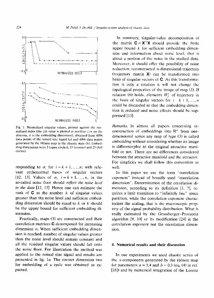
Fig. 1. Normalized singular values, plotted against the nor-

malized index (the jth value is plotted at position j/n on the

abscissa, n is the embedding dimension), obtained from 4096

data points of the noised sine signal (a) and 4096 data points

generated by the H&on map in the chaotic state (b). Embed-

ding dimensions were 5 (open circles), 15 (crosses) and 25 (full

circles).

responding to U, for i = k + 1,. . . , n; with rele-

vant orthonormal bases of singular vectors

[12, 131. Values of a,, i = k + l,..., n, in the

so-called noise floor should reflect the noise level

in the data [12, 131. Hence one can estimate the

rank of C as the number k of singular values

greater than the noise level and sufficient embed-

ding dimension should be equal to k or k should

be the upper bound for sufficient embedding di-

mension.

Practically, maps (3) are constructed and their

correlation matrices C decomposed for increasing

dimension n. When sufficient embedding dimen-

sion is reached, number of singular values greater

than the noise level should remain constant and

all the residual singular values should fall onto

the noise floor. For illustration the method was

applied to the noised sine signal and results are

presented in fig. la. The correct dimension two

for embedding of a cycle was obtained as ex-

pected.

In summary, singular-value decomposition of

the matrix C = XTX should provide the finite

upper bound k for sufficient embedding dimen-

sion and information about noise level, that is

about a portion of the noise in the studied data.

Moreover, it should offer the possibility of noise

reduction: reconstructed n-dimensional trajectory

(trajectory matrix X) can be transformed into

basis of singular vectors of C. As this transforma-

tion is only a rotation it will not change the

topological properties of the image of map (3). If

relation (6) holds, elements WY of trajectory in

the basis of singular vectors for i = k + 1, . . . , n

could be discarded so that the embedding dimen-

sion is reduced and noise effects should be sup-

pressed [ 131.

Remarks. In almost all papers concerning re-

construction of embeddings into R” from one-

dimensional series any map of type (3) is called

embedding without considering whether its image

is diffeomorphic to the original attractive mani-

fold or not. There are no differences considered

between the attractive manifold and the attractor.

For simplicity we shall follow this convention as

well.

In this paper we use the term “correlation

exponent” instead of broadly used “correlation

dimension”. Determination of the correlation di-

mension, according to its definition [l, 71, re-

quires a limit transition to “infinitely fine” space

partition, while the correlation exponent charac-

terizes the scaling, that is the macroscopic prop-

erty of the signal probability distribution. What is

really estimated by the Grassberger-Procaccia

algorithm [9, 101 or its modification [24] is the

correlation exponent not the correlation dimen-

sion.

4. Numerical results and their discussion

In our experiments we used chaotic series of

the x-components generated by the H&on map

for parameters a = 1.4 and b = 0.3 (eq. (4) in ref.

[16]) and by numerical integration of the Lorenz

M. PaluS, I. Duo%k /Singular-system analysis of chaotic data 225

-23.5k a NORMALIZED INDEX 1.

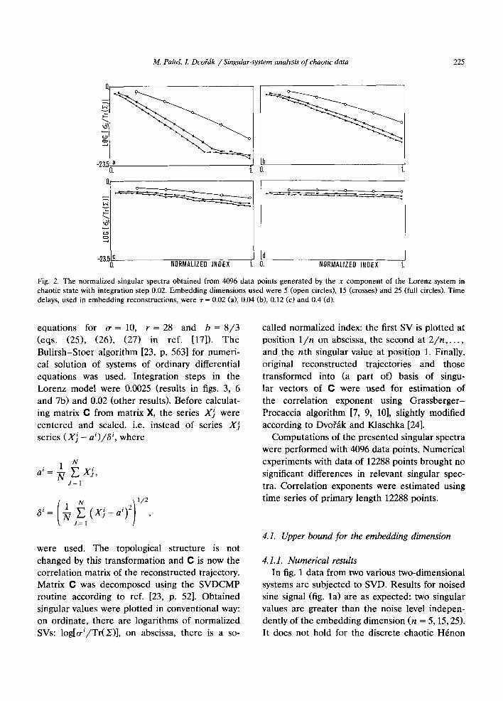
Fig. 2. The normalized singular spectra obtained from 4096 data points generated by the x component of the Lorenz system in

chaotic state with integration step 0.02. Embedding dimensions used were 5 (open circles), 15 (crosses) and 25 (full circles). Time

delays, used in embedding reconstructions, were 7 = 0.02 (a), 0.04 (b), 0.12 Cc) and 0.4 Cd).

0 0

-

0 1.

equations for u = 10, r = 28 and b = 8/3 (eqs. (251, (261, (27) in ref. [17]). The Bulirsh-Stoer algorithm [23, p. 5631 for numeri- cal solution of systems of ordinary differential equations was used. Integration steps in the Lorenz model were 0.0025 (results in figs. 3, 6 and 7b) and 0.02 (other results). Before calculat- ing matrix C from matrix X, the series Xj were centered and scaled. i.e. instead of series Xj series (Xj - ~‘)/a’, where

were used. The topological structure is not changed by this transformation and C is now the correlation matrix of the reconstructed trajectory.

Matrix C was decomposed using the SVDCMP routine according to ref. [23, p. 521. Obtained singular values were plotted in conventional way: on ordinate, there are logarithms of normalized SVs: log[a’/TrW, on abscissa, there is a so-

called normalized index: the first SV is plotted at position l/n on abscissa, the second at 2/n,. . . ,

and the nth singular value at position 1. Finally, original reconstructed trajectories and those transformed into (a part of) basis of singu- lar vectors of C were used for estimation of the correlation exponent using Grassberger- Procaccia algorithm 17, 9, 101, slightly modified according to Dvo%k and Klaschka [24].

Computations of the presented singular spectra were performed with 4096 data points. Numerical experiments with data of 12288 points brought no significant differences in relevant singular spec- tra. Correlation exponents were estimated using time series of primary length 12288 points.

4.1. Upper bound for the embedding dimension

4.1.1. Numerical results In fig. 1 data from two various two-dimensional

systems are subjected to SVD. Results for noised sine signal (fig. la) are as expected: two singular values are greater than the noise level indepen- dently of the embedding dimension (n = $1525). It does not hold for the discrete chaotic H&on

226 M. Palu.?, I. DwGk /Singular-system analysis of chaotic dater

-23.5 c 0. NORMALIZED INDEX 1.

r

I

NORMALIZED INDEX i.

Fig. 3. The normalized singular spectra obtained from 4096 data points generated by the x-component of the Lorenz system in

chaotic state with integration step 0.0025. Embedding dimensions used were 5 (open circles), 15 (crosses) and 25 (full circles). Time

delays, used in embedding reconstructions. were 7 = 0.02 (a), 0.04 (b), 0.12 Cc) and 0.4 Cd).

map (fig. lb): no noise floor is detected here;

from the viewpoint of SVD it is classified either

as a pure noise or as a deterministic system of

high dimension and not as the two-dimensional

system which it is actually.

Figs. 2 and 3 present results of SVD applica-

tion to data from the continuous Lorenz system.

The number of singular values greater than the

noise level increases with increasing embedding

dimension, n = 5,15,25, or, more frequently, no

noise floor is detected. (Influence of time delay

and integration step - “sampling frequency” - on

singular spectra, depicted on the above figures,

will be discussed further.)

Influences of data precision and of a defined

amount of noise in the data on the singular

spectra were studied next. The same data from

the x-component of the Lorenz system were gen-

erated with various precisions: 6, 10, 14 and 18

bits, and 18-bit data were jammed by Gaussian

noise so that contents of about 10% and 30% of

noise in the data were obtained. Fig. 4a confirms

the report of Mees et al. [13] that the higher the

precision the more singular values are greater

than noise level (noise floor is sinking with in-

creasing precision of data). Also an increase of

the amount of noise brings more singular values

to fall onto the noise floor-see fig. 5a. It seems

that the number of singular values over the noise

floor depends on numerical accuracy, precision of

the data and amount of noise in the data rather

than on intrinsic dynamical structure of the sys-

tem under study. (Influence of time delay r on

the singular spectra will be discussed further.)

We should note, however, that each of the “up-

per bounds” (numbers of singular values above

the noise floor) obtained is sufficient to embed

faithfully the attractor. Since experimentalists

need saturation of the value in question on well-

defined and possibly the lowest upper bound in

case the dimension of the studied system is un-

known, SVD is not too reliable for this purpose.

4.1.2. Discussion of results

Let us try to explain the obtained results. Let k

be the sufficient embedding dimension in previ-

ously defined sense, e.g. for data from the Lorenz

system k = 3 (for proper time delay T, see fur-

ther). Let embedding dimension n be n 2 2k. It

can possibly occur that there are two subspaces of

M. PaluS, I. DuoGk /Singular-system analysis of chaotic data 227

---P-.

---b.. __

NORMALIZED INDEX 1.

Fig. 4. The normalized singular spectra computed from 4096

data points generated by the x component of the Lorenz

system in chaotic regime with integration step 0.02. In each

case the embedding dimension was 25. The four different

spectra were obtained from data of various precisions: 6, 10,

14 and 18 bits (reading from top to bottom). Time delays,

used in embedding reconstructions, were r = 0.02 (a) and 0.12

(b). In case of r = 0.12 (b) the singular spectra are practically

undistinguishable whatever the data precision is.

R” containing diffeomorphic images of the origi-

nal attractive manifold. As a diffeomorphism is a

relation of equivalence, these two images are

mutually diffeomorphic, i.e. relations:

X’=f’(X’,X2 )...) Xk),

for i=k+ l,...,n (7)

and their inverses hold. (The superscript denotes

again the component index, time index or argu-

ment is not used for simplification of formulas.)

Diffeomorphic relations f’ need not be linear so

that in embedding (3) more than k, possibly even

n, linearly independent components can be found.

As correlation is measure of a linear dependence

[14, 22, 251 and correlation (or covariance) matrix

C reflects the structure of this linear dependence,

it is clear that the singular-value decomposition

of C, extracting the number of linearly indepen-

-25.z0a NORMALIZEO INDEX 1.

-25.2 b 0. NORMALIZED INDEX 1.

Fig. 5. The normalized singular spectra computed from 4096

data points generated by the x component of the Lorenz

system in chaotic state with integration step 0.02 and recorded

with precision 18 bits. In each case the embedding dimension

was 25. The three different spectra were obtained from data

jammed by different portions of the Gaussian noise: 30%,

10% and no noise (reading from top to bottom). Time delays,

used in embedding reconstructions, were r = 0.02 (a) and 0.12

(b). In case of T = 0.12 (b) the singular spectra are practically

undistinguishable whatever the portion of noise in data is.

dent components in the embedding, cannot dis-

cover the true dimensionality of the system under

study. Especially, as a one-dimensional chaotic

time series has a finite correlation length 7, (its

autocorrelation function is usually exponentially

decreasing [l]), any number of linearly indepen-

dent delayed series can be constructed (up to

some practical bound given by precision, sam-

pling frequency etc.) using time delay T > TV. As a

consequence the SVD procedure gives unbound-

edly increasing number of singular values greater

than the noise level or no noise level is obtained

in singular spectrum at all.

4.1.3. The role of the “window length” In all our experiments with SVD, except of

those depicted in fig. 6, when we increased em-

bedding dimension n, we kept constant time delay 7. Alternatively, Broomhead and King [12] pro-

228 M. PaluS, I. Dr,oGk /Singular-system unalyxis of chaotic dutu

Fig. 6. The normalized singular spectra computed from 4096

data points generated by the x component of the Lorenz

system in chaotic state with integration step 0.0025 and

recorded with precision 20 bits. Embedding dimensions were

n = 10 (open circles), 20 (crosses) and 40 (full circles). The

constant “window lengths” 7, = 0.1 (a), 0.2 (b) and 0.3 Cc)

were used, i.e. time delay T, used in particular embedding

reconstruction. was 7 = 7*/n.

posed to keep constant a so-called window length

7, = nr, i.e. when we increase dimension n, delay

T must proportionally decrease. According to our

experience this is exactly the way which can bring

“false positive” results when SVD is applied: As

a time series obtained from a continuous chaotic

system has bounded but usually nonzero correla-

tion length 0 < 7, +K 03 [l], for given window length

a limited number of linearly independent delayed

series can be constructed and any other series

from the window is correlated with previous ones.

As a consequence, we can state the following

conjecture: For any k E N there is a window

length T,.~ so that keeping constant T~,~ the

number k of singular values greater than the

noise level will remain constant for n 2 k. (There

are again some numerical restrictions.) This phe-

nomenon is illustrated in fig. 6. Using the same x

series of the Lorenz system and keeping constant

window lengths T,,,,~ = 0.1, r,,h = 0.2 and r,, x =

0.3, constant numbers of “deterministic” singular

values k = 4 - 5, 6 and 8, respectively, were ob-

tained.

There are examples quoted in ref. [12] where a

proper choice of window length (around the cor-

relation time of the signal) brings satisfactory

results. These examples document that the con-

stant window length-if ever used-should be

chosen and used with utmost care.

4.2. SVD and noise control

4.2.1. Numerical results

Discovered dependence of the noise level in

singular spectra on data precision (fig. 4a) and on

the amount of noise in the data (fig. 5a) led some

authors [13] to assume that singular-value decom-

position could be used as an efficient tool for

detecting the amount of noise in the studied data.

Comparing parts (a) and (b) of figs. 4 and 5 we

can see that the detected noise level and even its

occurrence in a singular spectrum depends on

time delay T used in an embedding construction

rather than on precision of the data or on the

actual amount of noise in the data: Results pre-

sented in figs. 4b and 5b were obtained by com-

putations in the same conditions as those in figs.

4a and 5a, respectively; except of time delay T

which is T = 0.02 for spectra given in figs. 4a and

5a and r = 0.12 for spectra in figs. 4b and 5b. The

singular spectra in figs. 4b and 5b are practically

the same whatever the precision of data or the

amount of noise in the data are.

4.2.2. Discussion of results

Occurrence of the noise level in the singular

spectrum of the correlation matrix of an embed-

M. PaluS, I. Dr:oGk /Singular-system analysis of chaotic data 229

ding means that there are linearly dependent components in the embedding, or, in other words, that components of the embedding are corre- lated. Correlation of two identical but lagged series (which is the case in the Takens’ embed- ding method) depends on lag T and on the sam- pling rate of the signal (on the integration step in the generated data). Occurrence of a noise floor implies the possibility that a signal is oversampled and certainty that the lag T is less than a “proper” time delay 7p (see further) and/or the correla- tion length T, of the series. (Condition T,, > T, is not always necessary because even actual compo- nents of the system can be slightly correlated.)

The theory [5] gives broad possibility for setting the value of time delay T in the embedding construction. When the embedding dimension is sufficient [20, 211 the maps of type (2) and (3) are (diffeomorphic) embeddings generically. This holds for function u, flow 4 in (2) and lag r in (3). In general, an object from some set or space of objects is generic if it is the element of the intersection of countably many open sets, dense in this space. In experimental practice, however, the situation is different and map (3) is (diffeo- morphic) embedding usually for drastically re- duced subset of theoretically accepted values of 7.

Based on numerical experience we could state that the time delay 7p is “proper” when the image of the map (3) constructed using 7p is diffeomorphic with the original geometry of the system attractive manifold and the embedding dimension is not greater than the smallest suffi- cient embedding dimension. Embeddings con- structed with T < 7p are wrong or improper in the following way: a diffeomorphic image of the sys- tem attractor is reached in R” with dimension n higher than the embedding dimension, which is sufficient for 7p and computations of e.g. correla- tion exponent are superfluously complicated. In the worst case, whatever the dimension II is, the components of map (3) are so strongly correlated that estimations of CE are heavily biased down- wards or even tend to unity (fig. 7a). On the other

EMBEDDING DIMENSION

0.5GP . * . . I . . * I - , . . 5. 10. 15.

EMBEODING DIMENSION

Fig. 7. Estimates of correlation exponent from 12288 data

points of the x components of the Lorenz attractor dynamics

plotted against the embedding dimension. (a) Dependence of

the CE estimation on time delay 7, used in the embedding

reconstruction, for 7 = 0.12 (open circles), 0.04 (full circles)

and 0.02 (crosses). Data were generated with integration step

0.02 and recorded with precision 20 bits. (b) Dependence of

the CE estimation on the integration step 7i of the data

generation (“sampling frequency”) for -ri = 0.02 (open circles)

and 0.0025 (full circles). Time delay 7 = 0.12. Horizontal lines

at positions 1.95 and 2.15 on the ordinate are frontiers of 5%

error of estimation.

hand, for T greater than some “greatest proper rP” the estimates of CE are overestimated.

There are several methods for determining the proper time delay rP. The most promising, ac- cording to our experience, is the method of the first minimum of mutual information [26] giving for our Lorenz series 7p = 0.12.

Further study of the dependence of singular spectra on lag T is depicted in figs. 2 and 3. Using T,, = 0.12 a noise floor disappears (figs. 2c and 3~). Comparing the numbers of singular values on the

noise levels in figs. 2a and 3a an influence of the

integration step (sampling frequency) on the sin-

gular spectra can be seen.

4.3. Test of the embeddings by CE computations

“Quality” of the above embeddings of the

Lorenz attractor for various T was studied using

the Dvoiak-Klaschka version [24] of the

Grassberger-Procaccia algorithm [9, 101 for esti-

mation of the correlation exponent (fig. 7). Using

data with integration step 0.02 and rp = 0.12

determined by the first minimum of mutual infor-

mation [26], according to our expectation, embed-

ding dimension n = 3 was found as sufficient and

unbiased value CE = 2.03 [ll] (with standard de-

viation less than 0.1) was obtained. For n > 3 CE

saturates (with slight random oscillations) on this

value. Using T = 0.04 CE is underestimated up to

n = 10-12, when the correct value is reached.

Delay T = 0.02, which seemed in previous compu-

tations so promising for the noise control, gives

so strongly correlated components of the embed-

ding that the value CE = 1 is estimated whatever

the dimension n of the embedding is (fig. 7a).

Using series with integration step 0.0025 and the

same series length as previously (N,, = 122881,

even for r,, = 0.12 CE is underestimated, proba-

bly due to correlations caused by “oversampling”

of the signal (fig. 7b).

4.4. SVD and noise reduction

4.4.1. Numerical experiment

Before further testing of the SVD applications,

let us summarize the results of the above discus-

sion: The aim of the attractor reconstruction from

a one-dimensional time series is to reconstruct an

uncorrelated embedding with the lowest possible

embedding dimension. (Slightly correlated com-

ponents are acceptable; a more general formula-

tion could be “to obtain the highest information

content in the lowest possible number of compo-

nents”.) Using the method of the first minimum

of the mutual information [26] and its generaliza-

tion [27] such embedding can be in principle

constructed. It seems that using the singular-value

decomposition loses its sense: with increasing em-

bedding dimension n we find no upper bound for

the number of linearly independent components.

No noise floor need to be detected and a frontier

between “deterministic” and “noise” components

in a singular spectrum need not be found. So that

using SVD as a noise reduction technique by reject-

ing the “noise” components of the embedding in

the basis of singular vectors is dubious. But, in

order to lead the discussion to the whole end, let

us suppose that one can know the sufficient em-

bedding dimension and wants to use SVD only

for the noise reduction.

Let us estimate CE for the Lorenz data jammed

with 10% of the Gaussian noise (with time delay

rp = 0.12). While for the same signal without noise

starting with n = 3 CE saturates approximately

on the expected value 2.03-2.08, presence of

noise causes overestimation of CE: for II = 3 CE

= 2.77 was obtained. (For n = 4 CE = 3.36, etc.)

If we insist on strict application of the algorithm

for CE estimation based on saturation of its val-

ues with increasing n, addition of noise blurs the

saturation and CE - strictly speaking - is not de-

fined. We can estimate, however, the value of CE

for each II and with the aforementioned signals

we can test the noise reduction ability of the

singular-value decomposition.

Embedding n/k in the following means that

an n-dimensional embedding was constructed and

its n X n correlation matrix C was decomposed.

The reconstructed trajectory was transformed into

the basis of singular vectors of C ordered accord-

ing to decreasing singular values. The first k

components of the transformed trajectory (corre-

sponding to the k largest singular values of C)

were used in CE estimations as proposed when

using SVD as the noise-reduction technique [13].

With the noise level in the singular spectrum

absent (fig. 2c) we tried to make use of the

previous experience:‘using rp = 0.12 for these data

the three-dimensional embedding could be suf-

ficient. Embedding 5/3 gave CE = 2.59, for 7/3

M. PaluS, I. Dl,ot%k /Singular-system analysis of chaotic data 231

CE = 2.61 and for 9/3 CE = 2.43 were obtained.

Overestimation was attenuated. Was it the effect

of noise reduction or not? We repeated these

computations for pure, not-noised data, which

gave for II = 3 CE = 2.03, n = 4 CE = 2.07, etc.,

as discussed in section 4.3 (fig. 7, T’, = 0.12). Em-

bedding 5/3 gave CE = 2.07, for 7/3 CE = 1.96

and for 9/3 CE = 1.77 were obtained. Results

from the embedding sequence n/3 are depicted

in fig. 8a. It can be seen that for n > 6 CE for

embeddings n/3 are underestimated. It seems

that SVD can reduce dynamical information

rather than noise.

4.4.2. Discussion of results In order to find a possible explanation of the

above phenomenon let us recall relations (7) and

propose the special form of them holds for some

indexes j~[k+ l,...,n]:

Xj=f’(X’,X’).

After SVD the first three components in the

singular-vector basis related to the three largest

singular values can be written as:

w’ =g’(X’, X’),

w” =gj(X’, X’), (8)

because singular values are given by the variance

of the transformed components [22, p. 5011 and

do not reflect the nonlinear dynamical structure

of the data. Functions g’, i = 1,2,3, can be non-

linear and the three components (8) can be lin-

early independent. But, on the other hand, these

three components can obtain only some two-

dimensional projection of the Lorenz attractor.

(Estimation of CE is 1.8.) It is clear that using all

the transformed components full embedding

(contained several times in the original embed-

ded trajectory) must be obtained. In order to

l$ . 5. 10. 15.

PRIMARY EMBEtIDING DIMENSION

NLiMBER OF COMPONENTS IN BASIS OF SINGULAR VECTORS

Fig. 8. Estimates of correlation exponent from 12288 data

points of the x component of the Lorentz attractor dynamics,

obtained from: (a) the first three components (related to the

three largest singular values) of the embedding in the basis of

singular vectors of the correlation matrix of primary (Takens’

time delay) embedding, depicted against relevant primary

embedding dimension; (b) the first k components (sorted

according to descending singular values) of the embedding in

the basis of singular vectors of correlation matrix of the

primary 1 l-dimensional embedding, depicted against the

number k of components used in the estimation. Each primary

embedding was reconstructed from ZO-bit data generated with

integration step 0.02, time delay r = 0.12. Horizontal lines at

positions 1.95 and 2.15 on the ordinate are frontiers of 5%

error of estimation.

verify this, CE was computed for the sequence of

embeddings 11/k, k = 1,2,. . . , 11 (fig. Sb). Fig.

8b illustrates that “full” - diffeomorphic embed-

ding is reached earlier-for k = 6.

As we mentioned above, this particular situa-

tion (no noise floor in the singular spectrum) is

not the case for noise reduction as described in

previous papers [13]. But this “enlarged” analysis

is a good illustration of the “nonlinear phantom”

haunting people accustomed to the linear world

only. Even in case of noise floor presence the

supra-noise (linearly independent) components

could be created only from one true dynamical

component which is mapped nonlinearly from

one linearly independent component to another.

And other true dynamical components (together

with their nonlinear “ghosts”) could be sup-

pressed onto the noise floor due to lower vari-

ance.

In order to bring more support for these con-

siderations, we studied dependence structure of

components of the embedding of the Lorenz at-

tractor in the basis of singular vectors obtained by

SVD of the correlation matrix of primary 1 l-

dimensional embedding (T,, = 0.12, as above). The

correlation function and mutual information

[26, 28, 291 were calculated. The components of

the singular basis were ordered, as usual, accord-

ing to descending singular values.

The mutual information I(n, y) is, in general, a

measure of the stochastic dependence of two

random variables X, y. Roughly speaking, it can

be taken as a generalization of the correlation

function to nonlinear dependence. (For more de-

tails see refs. [26, 28, 291.) Mutual information

(MI) is non-negative, zero is equivalent to inde-

pendent variables X, y. For a more vivid repre-

sentation of the results correlation functions in

fig. 9 are depicted in absolute values.

Correlation functions (CF) and mutual infor-

mation (MI) of couples of the series are displayed

as functions of lag T, 0 I T 5 2.0, albeit values of

CF and MI for T = 0 are of main interest here.

Figs. 9a and 9b reflect the dependence of the

first and the second, and the first and the third

singular basis components, relevant to the three

largest singular values of the correlation matrix of

the original embedding. Correlation functions for

T = 0 are due to orthogonality of the basis close

to zero. But it does not hold for mutual informa-

tion between the components (figs. 9a and 9b),

which are significantly greater than zero, i.e. the

components are not independent. The depen-

Fig. 0. Mutual information (full lines) and absolute VHIUCS ol

correlation functions (dashed lines) of the first and the second

(a). of the first and the third (h) and of the first and the yisth

components of the embedding in the hasis of singular vectora

(sorted xcording to descending singular values) of the corre-

lation matrix of the primary I I-dimensional embedding of the

Lorew attractor, reconstructed hy the samt‘ way as the cap-

tion in tig. 8 dcscrihes. The *scales of (‘F and MI are identical

accidentally.

dence level between the first and the sixth

components (see fig. 9~) is much lower. This

corresponds to the above findings that the first six

components provide again the diffeomorphic em-

bedding of the attractor (see fig. 8b). (Here WC

must remark that neither for the ideal embedding

one can expect fully independent components,

because even the original components of the sys-

tem under study are’tied by the particular trajec-

tory.)

M. Palui, I. DroGk /Singular-system analysis of chaotic data 233

5. Concluding discussion

Reliability of singular-value decomposition in reconstructing a strange attractor from a one- dimensional chaotic time series was extensively tested. SVD, an effective method in discovering the linear structures in the data under study, can be misleading when nonlinear structures are of interest. Hence it can be hardly useful for de- termining an upper bound for the embedding dimension of the system attractor, or even dimen- sionality of the studied nonlinear system. Its role in noise control is questionable, too, because the so-called noise level and even its occurrence in singular spectra .depends on the sampling rate of the series and on the time delay used in the embedding reconstruction drastically more than on the precision of the measurement and the actual amount of noise in the data. Components of the orthonormal basis given by SVD are lin- early independent but can be strongly related in a nonlinear sense. As a consequence, the “most important” components, related to the largest singular values, can contain less dynamical infor- mation than the same number of components given by simple time delay method.

Presented criticism of SVD is not meant to refuse SVD technique as a whole or even de- nounce authors recommending application of SVD in nonlinear analysis. Though we in princi- ple agree with the majority of statements in ref. [131, we have no intention to evoke a discussion of the type “you criticize claims we never made” like in ref. [30, 311. But the results presented in our detailed analysis are warning to experimen- talists, trying to find dynamical structures or even to detect strange attractor in their data, to be precautious in SVD applications and especially in interpreting the results it yields.

While application of SVD in reconstructing an attractor from a one-dimensional time series by the time-delay method is questionable, it may be of great importance when multi-dimensional time series are registered [32]. Neither in this case

must we forget that nonlinearities in the data can distort the results.

Nonlinear relations in dynamical data are usu- ally equivalent to the curvature of the relevant attractive manifold. However, a manifold with nonzero curvature is locally flat. This fact was the inspiration for applying SVD locally, i.e. on a subset of trajectory confined to a neighborhood of selected points 133, 341. At the first sight this approach, in general not a new one (using local decomposition for estimating intrinsic dimension- ality of data was proposed by Fukunaga and Olsen [35] twenty years ago for general data without any concept of dynamical systems), seems to be promising even for determining the actual dimension of the attractive manifold. But, analyz- ing experimental data, many questions appear, like “is the local subset local enough?“, or “what is the noise effect in local case?“, etc. Therefore several authors try to use local SVD together with some statistical or informational criteria for estimating the number of deterministic compo- nents in the singular spectra [36, 371.

SVD is surely an established method of signal analysis, but it should be applied with caution. Also results it provides must be interpreted with care. Improper use of singular-value decomposi- tion (like that of Grassberger-Procaccia or any other algorithm) can bring misleading results in- terpreted like a (false) discovery of a strange attractor in any data. We are afraid that at least a part of recently published papers, alleging detec- tion of chaos, are based on misinterpreted re- sults, which cause “inflation” of the scientific value of this approach and jeopardize the pres- tige of deterministic chaos theory for experimen- tal data analysis.

Acknowledgement

The authors thank V. Albrecht and L. Pecen for stimulating discussions and M. Pipilka for assistance with figures.

References

[l] H.G. Schuster, Deterministic Chaos: An Introduction,

(Physik, Weinheim, 1984).

[2] P. Schuster, ed., Stochastic Phenomena and Chaotic Be-

haviour in Complex Systems, Springer Series in Synerget-

its, Vol. 21 (Springer, Berlin, 1984).

[3] P.E. Kloeden and A.1. Mees, Chaotic phenomena, Bull.

Math. Biol. 47 (1985) 697.

[4] P. Cvitanovic. ed., Universality in Chaos (Hilger, Bristol,

1984).

[5] F. Takens, Detecting strange attractors in turbulence, in:

Dynamical systems and turbulence, Warwick, 1980, Lec-

ture Notes in Mathematics No. X98, eds. D.A. Rand and

D.S. Young (Springer, Berlin, 1981) p. 366.

[6] G. Mayer-Kress, ed., Dimensions and Entropies in

Chaotic Systems (Springer, Berlin, 19861.

[7] P. Grassberger and I. Procaccia, Dimensions and en-

tropies of strange attractors from a fluctuating dynamics

approach, Physica D 13 (1984) 34.

[S] P. Grassberger and I. Procaccia, Estimation of the Kol-

mogorov entropy from a chaotic signal, Phys. Rev. A 28

(1983) 2591.

[9] P. Grassberger and I. Procaccia, On the characterization

of strange attractors, Phys. Rev. Lett. 50 (1983) 346.

[lo] P. Grassberger and I. Procaccia, Measuring the

strangeness of strange attractors, Physica D 9 (1983) 189.

[ll] P. Grassberger, Estimating the fractal dimensions and

entropies of strange attractors, in: Chaos, ed. A.V. Holden

(Manchester Univ. Press, Manchester, 1986) p. 291.

[12] D.S. Broomhead and G.P. King, Qualitative dynamics from experimental data, Physica D 20 (1986) 217.

[13] A.I. Mees, P.E. Rapp and L.S. Jennings, Singular-value decomposition and embedding dimension, Phys. Rev. A

36 (1987) 340.

[14] A.M. Fraser, Reconstructing attractors from scalar time

series: A comparison of singular system and redundancy

criteria, Physica D 34 (1989) 391.

[15] A. Brandstater, H.L. Swinney and G.T. Chapman, Char-

acterizing turbulent channel flow, in: Dimensions and

Entropies in Chaotic Systems, ed. G. Mayer-Kress

(Springer, Berlin, 1986) p. 150.

[16] M. Henon, A two-dimensional mapping with strange

1171

[I81

]I91

]201

attractor, Comm. Math. Phys. 50 (1976). 69.

E.N. Lorenz, Deterministic nonperiodic flow, J. Atmos. Sci. 20 (1963) 130.

E. Kamke, Differentialgleichungen Losungsmethoden

und Liisungen (Leipzig, 1959) (in Russian: Nauka,

Moscow, 1971).

V.I. Arnold, Ordinary Differential Equations (MIT Press,

Cambridge, 1973).

H. Whitney, Differentiable manifolds, Ann. Math. 37

(1936) 645.

]211

]221

]231

[241

]251

[261

I271

WI

[291

J. Palis Jr. and W. de Melo, Geometric Theory of Dy-

namical Systems, An Introduction (Springer. New York.

1 Y82).

C.R. Rao. Linear Statistical Inference and Its Applica-

tions. (Wiley. New York, 1965).

W.H. Press, B.P. Flannery, S.A. Teukolsky and W.T.

Vetterling, Numerical Recipes: The Art of Scientific

Computing (Cambridge Univ. Press, Cambridge, 19X6). I. Dvoiik and J. Klaschka. Modification of the

GrassbergerProcaccia algorithm for estimating the cor-

relation exponent of chaotic systems with high embed-

ding dimension, Phys. Lett. A 14.5 (1990) 225.

M.M. Rao, Harmonizable. Cramer and Karhunen classes

of processes, Handbook of Statistics. Vol. 5. eds. E.J.

Hannan, P.R. Krishnaiah and M.M. Rao (Elsevier, Ams-

terdam. 1985) p. 279.

A.M. Fraser and H.L. Swinney. Independent coordinates

for strange attractors from mutual information. Phys.

Rev. A 33 (1986) 1134.

A.M. Fraser, Information and entropy in strange attrac-

tors. IEEE Trans. Information Theory 35 (lY89) 245.

R.G. Gallager, Information Theory and Reliable Com-

munication (Wiley, New York. 1968).

S. Kullback. Information Theory and Statistics (Wiley,

New York, 1959).

[30] D.S. Broomhead. R. Jones and G.P. King. Comment on “Singular-value decomposition and embedding dimen-

sion”, Phys. Rev. A 37 (1988) 5004.

[31] A.I. Mees and P.E. Rapp. Reply to “Comment on ‘Singu-

lar-value decomposition and embedding dimension”,

Phys. Rev. A 37 (198X) 5006.

[32] M. PaluS, 1. Dvoiik and I. David. Remarks on spatial

and temporal dynamics of EEG, in: Mathematical Ap-

proaches to Brain Functioning Diagnostics. eds. I. Dvo%k

and A.V. Holden (Manchester Univ. Press. Manchester,

1991) p. 36’).

[33] D.S. Broomhead, R. Jones and G.P. King. Topological dimension and local coordinates from time series data,

J. Phys. A 20 (1987) LS63.

[34] E.R. Pike, Singular system analysis of time series data,

in: Computational Systems - Natural and Artificial, ed.

H. Haken (Springer, Berlin, 19X7) p. X6.

[35] K. Fukunaga and D.R. Olsen, An algorithm for finding

[x61

1371

intrinsic dimensionality of data. IEEE Trans. Computers

c-20 (1971) 176.

A. Gael, S.S. Rao and A. Passamante, Estimating local

intrinsic dimensionality using thresholding techniques, in:

Measures of Complexity and Chaos, eds. N.B. Abraham. A.M. Albano, A. Passamante and P.E. Rapp (Plenum Press, New York, 1989) p. 125.

A. Passamante, T. Hediger and M.E. Farrell, Analysis of

local space/time statistics and dimensions of attractors using singular value decomposition and information theo-

retic criteria, in: Measures of Complexity and Chaos. eds.

N.B. Abraham, A.M. Albano, A. Passamante and P.E.

Rapp (Plenum Press, New York. 19X9) p. 173.