Singular Foci of Planar Linkages

Charles W. Wampler

General Motors Research & Development, Mail Code 480-106-359,30500 Mound Road, Warren, MI 48090-9055, USA

Abstract

The focal points of a curve traced by a planar linkage capture essential informationabout the curve. Knowledge of the singular foci can be helpful in the design ofpath-generating linkages and is essential to the determination of path cognates.This paper shows how to determine the singular foci of planar linkages built withrotational links. The method makes use of a general formulation of the tracing curvebased on the Dixon determinant of loop equations written in isotropic coordinates.In simple cases, the singular foci can be read off directly from the diagonal ofthe Dixon matrix, while the worst case requires only the solution of an eigenvalueproblem. The method is demonstrated for one inversion each of the Stephenson-3six-bar and the Watt-1 six-bar.

Key words: Focal points, singular focus, Foci: singular, Linkages: planar, isotropiccoordinates, Dixon determinant

1 Introduction

Singular foci play a central role in the kinematics of four-bar coupler curves.For example, in 1875, Roberts [7] proved that every four-bar curve is triplygenerated, that is, traced by three distinct four-bar linkages. This proof wasnonconstructive, but Cayley [2] soon followed with a concrete constructionthat, given one four-bar, derives the other two cognates. These are now knownas Roberts cognates [1, pp. 339-341] [4]. Roberts’ Theorem hinged on the de-termination that a four-bar coupler curve has three singular foci. These threefoci, two of which are simply the fixed pivots of the linkage, define the “focaltriangle,” a triangle that is geometrically similar to the coupler triangle.

Email address: charles.w.wampler@gm.com (Charles W. Wampler).

Preprint submitted to Elsevier Science 22 June 2004

Despite the passing of over a century of active kinematic research, it seemsthat the foci of multiloop planar linkages have never been determined. Thispaper presents a method of finding the singular foci of any curve traced outby a planar linkage built with rotational joints. The approach uses the ex-pression for the tracing curve from [11], based on the Dixon determinant andisotropic coordinates . This leads to an algorithm for numerically determiningthe singular foci, which either appear directly on the diagonal of the Dixonmatrix, or in worst case, are given by eigenvalues of a matrix extracted fromthe Dixon matrix. In the case that a singular focus appears with multiplicitygreater than one, a method is given for determining its correct multiplicity.

One reason that the singular foci of multiloop linkages have not been stud-ied is that the polynomial describing the tracing curve is quite complicated.Although derivations had been found for each of the six-bar linkages [9], un-til recently, there did not exist a method for deriving these polynomials forgeneral linkages. This limitation is overcome by the general formulations in[6,10,11] for solving input/output problems: each of these can be adapted toproduce tracing curve polynomials. The last of these, [11], gives the tracingcurve equation in a particularly convenient form for studying the singular foci.The elegance of this approach is marred by the inclusion in some cases of anextraneous factor. A by-product of the current study is the determination ofthis factor, so that it can be cancelled out.

As in Roberts’ work, one of the main applications of focal points is the deter-mination of path cognates, linkages that generate the same curve. In [8], Rothgave geometric constructions for deriving path cognates of certain linkages.These constructions demonstrate existence of path cognates, but do not bythemselves prove that all cognates have been found. For completeness results,Roth turned to an algebraic analysis of the coefficients of the tracing curveand obtained completeness results for several geared five-bar linkages. In thispaper, we will show that matching the singular foci is equivalent to matchingthe coefficients of the terms of highest bidegree, as defined herein.

Constructions for path cognates of all of the six-bar linkages are known [4].(Cognates for body guidance and for function generation are also given in [4],but we do not discuss these in this article.) As in Roth’s work, these construc-tions, which make no overt use of the singular foci, show the existence of pathcognates but do not establish completeness. The new understanding of singu-lar foci brought out in this paper will be key to the complete determinationof path cognates in future work.

The paper proceeds as follows. First, in §2 we review some basic facts aboutthe geometry of the plane, and in particular the isotropic points of the plane.Then, §3 presents the definition of singular foci of a curve and shows that theseare determined by the terms of highest bidegree in the curve’s equation. This

2

observation leads in §4 to a determination of the singular foci from the Dixondeterminant form of tracing curve equations. Section 5 briefly discusses howthe methodology can be extended to treat mechanisms that include prismaticjoints. A final section, §6, gives numerical results for a Stephenson-3 six-barand a Watt-1 six-bar.

2 Background

In this section, some basic facts concerning isotropic points and one- andtwo-homogeneous treatments of the plane are reviewed. Related expositorymaterial can be found in [12]. An algebraic concept, called a support poly-nomial, is also introduced. All of these concepts are useful in working withsingular foci, as we will see in the §3.

2.1 One-homogenization of the plane

The most common method of accounting for how plane curves “meet infinity”is to consider a one-homogenization of the plane. When classical texts in ge-ometry or kinematics speak of “the line at infinity” and related concepts, theyoften assume this model of infinity without stating so. We first review thisconcept for Cartesian coordinates and isotropic coordinates, and then look atthe isotropic points at infinity.

2.1.1 Cartesian coordinates

Let the Cartesian coordinates of the plane be (x, y). Many results in geom-etry and kinematics become simpler if one extends the plane to include aline at infinity, having one point for each direction in the plane. The newspace is represented by homogeneous coordinates [X,Y,W ], where the brack-ets signify that only the ratios of the coordinates matter. (We do not allowall three coordinates to be zero simultaneously.) For finite points, W 6= 0, thecorrespondence between the two is (x, y) = (X/W, Y/W ). In addition to thefinite points, the new space has points at infinity, defined by W = 0. Sincethis is a linear equation, these points collectively form the line at infinity.Considering all of the coordinates to take on complex number values, math-ematicians call (x, y) ∈ C2 the two-dimensional complex Cartesian space andcall [X, Y, W ] ∈ P2 the two-dimensional complex projective space.

The correspondence between finite points of the two spaces can be used toderive from a polynomial f(x, y), its one-homogenization F (X,Y,W ). To do

3

so, make the substitution (x, y) = (X/W, Y/W ) and clear denominators bymultiplying by W d, where d is the degree of f . For finite points, the solutionsto f = 0 and F = 0 are identical, but F−1(0) additionally contains solutionsat infinity.

2.1.2 Isotropic coordinates

For most derivations, it turns out that a linear change of coordinates to(p, p) = (x + iy, x − iy) is very convenient. For real (x, y), this just replacesthe Cartesian plane with the complex plane, considering the x and y axes asthe real and imaginary directions, respectively. The pair of coordinates (p, p)are known as the isotropic coordinates of the plane. It is tempting to considerp as the complex conjugate of p, as it plays this role whenever x and y arereal. However, just as we allow Cartesian coordinates x and y to take on com-plex values, we correspondingly must consider points where p and p are notcomplex conjugates 1 .

The one-homogeneous completion of the plane in isotropic coordinates, whichwe write as [P, P ,W ] ∈ P2, follows similarly to the Cartesian case, using thecorrespondence (p, p) = (P/W, P/W ).

2.1.3 Isotropic points I and J

In any treatment of rigid-body motion, the concept of distance is fundamental.In Cartesian coordinates, the squared distance between points (x, y) and (a, b)is d((x, y), (a, b)) = (x− a)2 + (y − b)2.

Two real points are zero distance apart only if they are the same point. Thisis not true over the complexes; for example, d((1, i), (0, 0)) = 12 + i2 = 0. Infact, the squared distance factors as

d((x, y), (a, b)) = [(x− a) + i(y − b)][(x− a)− i(y − b)],

from which one sees that there are two lines of points that are zero distanceaway from (a, b), namely,

(x− a) + i(y − b) = 0 and (x− a)− i(y − b) = 0.

In a one-homogenization of these equations, one finds that these zero-distancelines, (X − aW ) + i(Y − bW ) = 0 and (X − aW )− i(Y − bW ) = 0, meet the

1 Note that x and y are real if, and only if, the corresponding p and p are complexconjugates. Thus, if p∗ = p, where ∗ denotes complex conjugation, we call (p, p) areal point even though p and p may be complex.

4

line at infinity, W = 0, at one point each. These are the so-called isotropicpoints

I = [1,−i, 0] and J = [1, i, 0].

Due to their kinship to distance, the isotropic points have a special relationshipto most of the curves studied in planar kinematics. Of particular note is the factthat every circle passes through the isotropic points. To see this, consider thatthe circle centered on (a, b) of radius r has the equation d((x, y), (a, b))−r2 = 0.When one-homogenized and intersected with W = 0, the radius becomesirrelevant, and we have the same situation as in the previous paragraph.

In isotropic coordinates, the squared distance between points (p, p) and (q, q)is

d((p, p), (q, q)) = (p− q)(p− q),

which reflects the fact that a complex vector times its own conjugate givesits squared magnitude. The factorization is apparent and one sees that inisotropic coordinates, the isotropic points are

I = [1, 0, 0] and J = [0, 1, 0].

Thus, the isotropic coordinates are seen to result from choosing coordinateaxes that align with the isotropic points. The simple form of the distancefunction and the isotropic points is the reason that isotropic coordinates oftenlead to simpler derivations than Cartesian coordinates. The remainder of thispaper will use isotropic coordinates exclusively.

2.2 Two-homogenization of the plane

There is another way to compactify the plane: we may introduce a separatehomogeneous coordinate for each of p and p. The new coordinates are writ-ten as ([P,W ], [P , W ]), where at least one coordinate in each of [P, W ] and[P , W ] must be nonzero. For all finite points, we have the correspondence(p, p) = (P/W, P /W ). The two-homogenization F (P, W, P , W ) of a func-tion f(p, p) is derived by making this substitution and clearing denominators.Mathematicians call [P, W ] ∈ P1 a one-dimensional complex projective space,and ([P, W ], [P , W ]) ∈ P1 × P1 is the cross product of two such spaces. Notethat the two-homogenization has singled out the coordinate axes as specialdirections. Accordingly, it is not generally useful to two-homogenize Cartesian

5

coordinates, but it turns out to be very useful to two-homogenize the isotropiccoordinates.

The two-homogenization of the plane, P1 × P1, has no effect on the geometryof finite points, but it radically alters the picture at infinity. There are nowtwo lines at infinity: W = 0 and W = 0. A line p − q = 0, parallel to thep-axis, two-homogenizes to P − qW = 0. It does not meet W = 0, but hitsW = 0 in the point ([q, 1], [1, 0]). Similarly, a line p − q = 0 meets infinity inthe point ([1, 0], [q, 1]). All lines not parallel to a coordinate axis meet infinityin the same point: ([1, 0], [1, 0]). If we try to associate points at infinity in theone-homogeneous treatment of the plane with those of the two-homogeneousisotropic treatment of the plane, we find that isotropic point I has been re-placed by the line W = 0, isotropic point J has been replaced by line W = 0,and all other points on the one-homogeneous line at infinity have collapsed tothe single point ([1, 0], [1, 0]). A nice illustration of this “blow up/blow down”process, which is one of the basic constructions in algebraic geometry, can befound in [5, ex.7.22].

An important consequence of the transformation into P1 × P1 is that twogeneral circles no longer meet at infinity. (In P2, they always meet at theisotropic points.) Instead, the two-homogenization of a circle with center (q, q)and radius r,

(P − qW )(P − qW )− r2WW = 0, (1)

hits the line W = 0 at ([1, 0], [q, 1]) and hits W = 0 at ([q, 1], [1, 0]). Thisshows that only concentric circles meet at infinity, which reflects the fact thatthey do not have finite points of intersection.

2.3 Support polynomials

Suppose that we have a polynomial

g(p, p) =∑

(j,k)∈Iαjkp

j pk,

where I is just the index set of all the terms appearing in the polynomial.Further, let Iuv denote the subset of indicies in I that maximize ju + kv,let duv = maxI(ju + kv) and let guv(p, p) =

∑(j,k)∈Iuv

αjkpj pk. The latter

is called the support polynomial of g for direction (u, v). In particular, g11

consists of the terms of maximal degree d = d11, g10 consists of the terms ofmaximal bidegree d10 in p, and g01 comprises the terms of maximal bidegreed01 in p. (Bidegree means the degree in one of the variables, treating the other

6

5 • • •4 • • • •3 • • • • •2 • • • • • •1 • • • • • •0 • • • • • •

0 1 2 3 4 5

@@

@@

@@

@@

g10

g01

g11

deg p

degp

Fig. 1. Monomials (plotted by their degrees) of a curve with degree d = 7, bidegreeb = 5, and circularity c = 2. The support polynomials g11, g10, and g01 are indicated.

variable as a constant.) These support polynomials are indicated in a plot ofthe monomials for a particular degree 7 polynomial in Fig.1.

For kinematics, we are interested in real curves. In Cartesian coordinates, theseare polynomials f(x, y) that have real coefficients, and hence f gives a realvalue whenever x and y are both real. Accordingly, the transformation of f toisotropic coordinates,

g(p, p) = f((p + p)/2, (p− p)/(2i)),

has real values whenever p and p are complex conjugates. This implies thatthe coefficients in g(p, p) obey the relation ajk = a∗kj, that is, terms appear incomplex conjugate pairs. Consequently, d10 = d01, so we may call b = d10 = d01

simply the bidegree of the curve. The terms may be shown in a plot of theirexponents as illustrated in Fig 1. Clearly, d ≥ b, and we call c = d − b ≥ 0the circularity of the curve. Curves with nonzero circularity are common inplanar kinematics.

Support polynomials determine the behavior of the curve at infinity. The one-homogenization G(P, P ,W ) = 0 of curve g(p, p) = 0 meets infinity at the rootsof G(P, P , 0). Setting the homogeneous coordinate W to zero annihilates allbut the terms of highest degree, hence

G(P, P , 0) = G11(P, P , 0) = g11(P, P ).

For bidegree b and circularity c, assuming that the coefficients αb,c = α∗c,b 6= 0,G11 contains the factor P cP c, so we have that the curve passes through eachof the isotropic points c times.

In a two-homogeneous formulation, the same curve g(p, p) = 0 hits infinityin the p direction at the roots of G10 and in the p direction at the roots ofG01, each of which is a degree c polynomial. The c appearances of each ofthe isotropic points in the one-homogeneous formulation have each become c(generally distinct) points at infinity in the two-homogeneous treatment. There

7

is one point on the line W = 0 at infinity in P1 × P1 for each line throughthe isotropic point I = [1, 0, 0] in P2, and a similar correspondence holdsbetween points on W = 0 and lines through J = [0, 1, 0]. A curve in P2 thatpasses through I along c different tangent directions will, after transformationinto P1 × P1, hit the line W = 0 in c distinct points. This separation of thetangent lines through I and J is precisely what makes the two-homogeneousformulation convenient for studying foci.

3 Foci and Singular Foci

We begin this section with the traditional definitions of a focal point and a sin-gular focal point. These definitions may seem at the outset a bit abstruse, butreconsidering them using isotropic coordinates, we will see that the definitionsbecome quite simple.

The traditional definition of a focal point assumes a one-homogeneous treat-ment of infinity, so that we may speak of the isotropic points I and J . Given analgebraic curve and a point, there will be a finite number of lines through thepoint that are also tangent to the curve. This fact also applies when the pointin question is an isotropic point, which is crucial to the following definitions[3].

Definition 1 A focal point of an algebraic curve in the plane is defined asthe point of intersection of a tangent through isotropic point I with a tangentthrough isotropic point J .

Definition 2 A singular focal point 2 of an algebraic curve in the plane isthe intersection of a tangent at isotropic point I with a tangent at isotropicpoint J .

Notice that a curve can have a singular focus only if it passes through theisotropic points; that is, it must have positive circularity.

The name “singular focus” is appropriate because such a point representsthe coalescence of several foci for nearby curves having the same degree butsmaller circularity. Suppose a curve of degree greater than one passes nearbut not through a point P . Locally, the curve looks like its osculating circle,and there are two nearly parallel tangents passing through P . As the curvedeforms continuously to pass through P , these two tangents coalesce into adouble tangent line. In the case that P is one of the isotropic points, the focion the the two tangents coalesce as well. It is also possible for a curve to pass

2 Bottema and Roth [1] note that singular foci are also sometimes called special,principal, or Laguerre foci.

8

through an isotropic point with zero curvature, which implies a multiple rootof order greater than two.

It is helpful to translate these geometric definitions into algebraic equations.Suppose that the curve is given by the equation f(p, p) = 0. Let (q, q) be apoint on the curve, hence

f(q, q) = 0. (2)

The line tangent to the curve at (q, q) is

fp(q, q)(p− q) + fp(q, q)(p− q) = 0, (3)

where fp and fp denote the partial derivatives of f with respect to p and p,respectively. Given (p, p), a simultaneous solution of Eqs.(2,3) for (q, q) deter-mines the point of tangency for a tangent through (p, p). Accordingly, we mayfind the foci of the curve by homogenizing these equations and substitutingthe isotropic points for (p, p). The homogenized tangent equation is

fp(q, q)(P −Wq) + fp(q, q)(P −Wq) = 0. (4)

For isotropic point I = [1, 0, 0], this becomes simply

fp(q, q) = 0. (5)

Let (qI , qI) be one of the solutions to the pair of equations (2,5). When sub-stituted back into Eq.3, this gives the equation for the tangent line as p = qI .Similarly, points of tangency for the tangents through J are the solutions ofEq.2 with fp(q, q) = 0. Denoting one such point as (qJ , qJ), the correspondingtangent line is p = qJ , and hence point (qJ , qI) is a focal point. If f(q, q) = 0 isa real curve, then we can obtain the real foci by pairing up each qJ with a qI

that is its complex conjugate. Due to this complex-conjugate relationship, oneonly needs to find the tangents through one of the isotropic points to obtainboth sets of tangents.

Example 1 Foci of an ellipse. An ellipse centered at the origin and alignedwith the coordinate axes has the equation x2/a2 + y2/b2 − 1 = 0. In isotropiccoordinates, this becomes

f(p, p) = (p + p)2/a2 − (p− p)2/b2 − 4 = 0.

Solving this simultaneously with fp(p, p) = 0 gives pI = ±√a2 − b2. Similarly,the tangents through J give pJ = ±√a2 − b2. These combine to give four

9

foci. In Cartesian coordinates, these are (x, y) = (±√a2 − b2, 0) and (x, y) =(0,±i

√a2 − b2). If a > b, the first of these gives a pair of real foci on the

x-axis, whereas for a < b, the second formula gives the real foci on the y-axis.

To determine the singular foci, we examine the tangency conditions as thepoint of tangency approaches an isotropic point. For the tangents at isotropicpoint I, the leading terms in q dominate in Eq.5, hence the qI coordinates ofthe singular foci are the roots of

(fp)10(1, qI) = 0. (6)

But (fp)10(1, qI) = (f10)p(1, qI) = bf10(1, qI), since differentiation with respectto p does not change which terms have the highest degree in p. Therefore, thesingular foci (qJ , qI) are the solutions to

f10(1, qI) = 0, f01(qJ , 1) = 0. (7)

Recall from the previous section that these roots are associated with the rootsat infinity in a two homogenization of the curve. This leads us to the followingtheorem.

Theorem 1 Let F (P, W, P , W ) be the two homogenization of a polynomialf(p, p). The singular focal points of f(p, p) = 0 are the points (p, p) = (qJ , qI),where qJ is any root of F of the form ([qJ , 1], [1, 0]), and qI is any root of Fof the form ([1, 0], [qI , 1]).

Example 2 Singular foci of a circle. At Eq.(1), we determined that the pointsat infinity of the two-homogenization of a circle with center (q, q) are

([q, 1], [1, 0]) and ([1, 0], [q, 1]).

Thus, the circle has its center as its only singular focus. Note that in light ofExample 1, considering the circle as a special ellipse, the center point is seento be the coalescence of four regular foci as the semi-major and semi-minoraxes, a and b, become equal.

4 Dixon Determinant

In [11], a general formulation is derived, using the Dixon determinant, forthe polynomial curve traced by any planar linkage with rotational joints. Themethod begins by writing the loop closure equations, using complex numbersto represent vectors in the plane. In these equations, let position vector p close

10

a loop around the tracing point. Then, for a one-degree-of-freedom mechanismhaving N = 2n links, there are n independent loop equations. These may bewritten, for k = 1, . . . , n as

ck0 +N−1∑

i=1

ckiθi + ckNp = 0, (8)

where cki is the vector of link i that appears in loop k, θi is the rotation forlink i. (Note: cki = 0 if link i is not in loop k.) We also have the conjugate setof equations, for k = 1, . . . , n,

c∗k0 +N−1∑

i=1

c∗kiθ−1i + c∗kN p = 0. (9)

We wish to eliminate all of the θi to obtain a single polynomial tracing curveequation in (p, p). The main result in [11] is written for input/output polyno-mials, but when applied to tracing curves, it reads as follows.

Theorem 2 [11]. The Dixon determinant for Eqs.(8,9), which is a necessarycondition for them to have a common solution, can be written as

f(p, p) = det(

D1p + D2 AT

A σ(D∗1p + D∗

2)

)= 0, (10)

where σ = (−1)n−1, D1 and D2 are diagonal and the elements of A obey therelation aij = σa∗ji. Matrices D1, D2, and A are all size m×m for some m ≤(

2n−1n

)and each is a homogeneous polynomial function of the link parameters

cki, c∗ki.

The dependence of D1, D2, and A on the link parameters may be determinedusing the procedure described in [11].

Since this is just a necessary condition, it is possible that f(p, p) contains anextraneous factor. But, if f = gh for polynomials f , g and h, then fuv = guvhuv;that is, the support polynomial for f in the (u, v) direction is the product ofthose for its factors. This implies that the singular foci of f are the union ofthose for its factors g and h. Thus, we may find all of the singular foci of thetracing curve by finding those of f and casting out any extraneous ones.

By Eq.7, to find the singular foci, we solve the support polynomial f01(qJ , 1) =0 consisting of the terms of f having maximal degree in p. Since a determinantis multilinear in its columns, we may find f01(p, p) by retaining in each col-umn only the terms of maximal degree in p. Each nonzero entry in D∗

1 standsalone in its column, but in any column where D∗

1 has a zero, the whole column

11

is constant and is therefore retained. For notational convenience, assume thecolumns and rows are ordered so as to place the nonzero entries into subma-trix D11 of D1 (and similarly for D∗

1), and partition the matrices D2 and Aaccordingly, to express f01(qJ , 1) = 0 as

det

D11qJ + D21 0 0 AT12

0 D22 0 AT22

A11 A12 σD∗11 0

A21 A22 0 σD∗22

= 0 (11)

Only one block in the third column is nonzero, so this may be reduced to

det(σD∗11) det

D11qJ + D21 0 AT12

0 D22 AT22

A21 A22 σD∗22

= 0. (12)

Numerical values for the singular foci can be obtained from this equation usingeigenvalue algorithms. Symbolic expressions can be obtained this way as well.

An important special case is when all entries on the diagonal of D1 are nonzero,so that only the upper left block of the above condition appears, the otherentries being empty. Thus the condition reduces to det(D1qJ +D2) = 0, whichimplies that the singular foci are simply

qJ = −diag(D−11 D2), (13)

where diag() extracts the diagonal of a matrix. Even when D1 has some zeroson the diagonal, causing A21 to be present in Eq.12, a condition similar toEq.13 applies to the subset of columns where A21 has all zero entries. Since Ais sparse, this condition comes into play often.

Since we are only concerned with real curves, the conjugate conditions giveqI = q∗J . So we need only solve either Eq.12 or Eq.13, as appropriate, to getqJ and find qI by conjugation.

Example 3 Singular foci of a four-bar.

Consider the four-bar linkage A0ADBB0, which is a sub-mechanism of thesix-bar in Fig.2. Letting p = ~OD, the loop equations are

a0 + a1θ1 + a2θ2 − p = 0

b0 + b2θ2 + b3θ3 − p = 0(14)

12

a0 b0c0

a1

a2

b3

b2

a5

b4

a4

A0 B0

C0

A

BC

D

E

O

2

4

Fig. 2. Four-bar (point D) and Stephenson-3 six-bar (point E) path-generatinglinkages

Applying the Dixon determinant and dividing common factors from each col-umn, we obtain the polynomial for the curve traced by coupler point D, ex-pressed in terms of isotropic coordinates (p, p) as the following determinantset to zero:

∣∣∣∣∣∣∣∣∣∣∣∣∣∣∣∣∣∣∣∣∣

p− b0 0 0 0 a2b3 −a2

0 d 0 −b3 0 −a1

0 0 p− a0 −b2 −a1b2 0

0 a2b3 −a2 p− b0 0 0

−b3 0 −a1 0 d 0

−b2 −a1b2 0 0 0 p− a0

∣∣∣∣∣∣∣∣∣∣∣∣∣∣∣∣∣∣∣∣∣

= 0, (15)

where

d = (p− a0)b2 − (p− b0)a2, d = (p− a0)b2 − (p− b0)a2.

Equation 13 applies, so the foci are

qJ = {b0, (a0b2 − b0a2)/(b2 − a2), a0}.

Two of these are the two fixed pivots A0 and B0, and the third is the vertex ofa triangle similar to the coupler triangle built on the fixed pivots. This is, ofcourse, a well-known result.

13

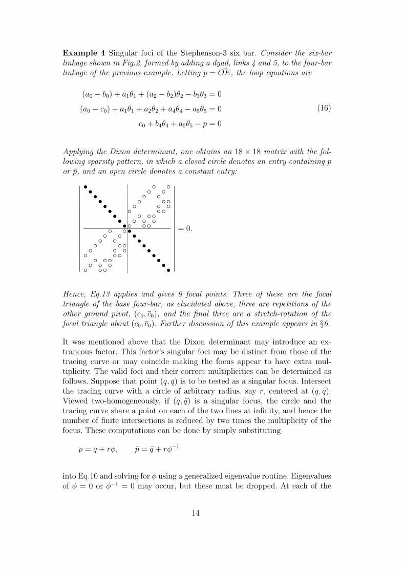
Example 4 Singular foci of the Stephenson-3 six bar. Consider the six-barlinkage shown in Fig.2, formed by adding a dyad, links 4 and 5, to the four-barlinkage of the previous example. Letting p = ~OE, the loop equations are

(a0 − b0) + a1θ1 + (a2 − b2)θ2 − b3θ3 = 0

(a0 − c0) + a1θ1 + a2θ2 + a4θ4 − a5θ5 = 0

c0 + b4θ4 + a5θ5 − p = 0

(16)

Applying the Dixon determinant, one obtains an 18× 18 matrix with the fol-lowing sparsity pattern, in which a closed circle denotes an entry containing por p, and an open circle denotes a constant entry:

∣∣∣∣∣∣∣∣∣∣∣∣∣∣∣∣∣∣∣∣∣

• ◦ ◦• ◦ ◦• ◦ ◦• ◦ ◦◦• ◦ ◦ ◦• ◦ ◦◦• ◦ ◦◦• ◦ ◦ ◦•◦ ◦◦◦ ◦•◦ ◦ •◦ ◦ •◦ ◦◦ •◦ ◦ ◦ •◦ ◦◦ •◦ ◦◦ •◦ ◦ ◦ •◦ ◦◦ •

∣∣∣∣∣∣∣∣∣∣∣∣∣∣∣∣∣∣∣∣∣

= 0.

Hence, Eq.13 applies and gives 9 focal points. Three of these are the focaltriangle of the base four-bar, as elucidated above, three are repetitions of theother ground pivot, (c0, c0), and the final three are a stretch-rotation of thefocal triangle about (c0, c0). Further discussion of this example appears in §6.

It was mentioned above that the Dixon determinant may introduce an ex-traneous factor. This factor’s singular foci may be distinct from those of thetracing curve or may coincide making the focus appear to have extra mul-tiplicity. The valid foci and their correct multiplicities can be determined asfollows. Suppose that point (q, q) is to be tested as a singular focus. Intersectthe tracing curve with a circle of arbitrary radius, say r, centered at (q, q).Viewed two-homogeneously, if (q, q) is a singular focus, the circle and thetracing curve share a point on each of the two lines at infinity, and hence thenumber of finite intersections is reduced by two times the multiplicity of thefocus. These computations can be done by simply substituting

p = q + rφ, p = q + rφ−1

into Eq.10 and solving for φ using a generalized eigenvalue routine. Eigenvaluesof φ = 0 or φ−1 = 0 may occur, but these must be dropped. At each of the

14

a0 b0

a1

a2

b2

a3

b3

a4

a5 b5

A0 B0

AB

C

D

E

P

O

2

3

5

Fig. 3. Watt-1 path-generating linkage

remaining finite, nonzero solutions, back substitute to find all the joint values(see [11] for details) and check these in the original loop equations. Let mq bethe number of valid solutions obtained in this way and let m be the numberfor an arbitrary test point. 3 Then, (m−mq)/2 is the multiplicity of (q, q) asa singular focus. A multiplicity of zero indicates that (q, q) is not a singularfocus. The following example illustrates the use of this technique.

Example 5 Singular foci of a Watt-1 six bar. Consider the Watt six-bar link-age shown in Fig.3. Denoting p = ~OP , the loop equations are

(a0 − b0) + a1θ1 + a2θ2 + a3θ3 = 0

b2θ2 + b3θ3 + a4θ4 + a5θ5 = 0

b0 − (a3 + b3)θ3 + b5θ5 − p = 0

(17)

Applying the Dixon determinant, one obtains an 18× 18 matrix with the fol-lowing sparsity pattern, in which a closed circle denotes an entry containing p

3 If either test gives solutions with multiplicity greater than one, a higher-orderanalysis may be required to determine m or mq.

15

or p, and an open circle denotes a constant entry:

∣∣∣∣∣∣∣∣∣∣∣∣∣∣∣∣∣∣∣∣∣

• ◦ ◦• ◦ ◦◦• ◦ ◦ ◦• ◦ ◦• ◦ ◦• ◦ ◦◦• ◦ ◦◦• ◦ ◦ ◦◦◦◦◦◦ ◦•◦ ◦◦ •◦ ◦ ◦ •◦ ◦ •◦ ◦ •◦ ◦◦ •◦ ◦◦ •◦ ◦ ◦ •◦◦◦ ◦

∣∣∣∣∣∣∣∣∣∣∣∣∣∣∣∣∣∣∣∣∣

= 0.

Because the final entry in D1 is zero, Eq.12 must be used. This results in amatrix with the following pattern, composed of the original upper left blockabove and only the last row and column of the rest:

∣∣∣∣∣∣∣∣∣∣∣∣

• ◦• ◦• ◦•••••◦◦◦◦ ◦

∣∣∣∣∣∣∣∣∣∣∣∣

= 0.

The fourth through eighth diagonal entries give focal equations directly, in thestyle of Eq.13, leaving an eigenvalue problem of the form

∣∣∣∣∣• ◦• ◦•◦◦◦◦◦

∣∣∣∣∣ = 0.

This gives three focal points. Among the combined eight focal points, qJ = b0

(that is, ground pivot B0 in Fig.3) appears four times. However, checking theintersections of the tracing curve with a circle centered on B0 reveals that B0

is only a triple singular focus. The Dixon determinant is thus seen to includea bilinear extraneous factor that has a singular focus (b0, b0). It turns out thatthe extraneous factor is just (p − b0)(p − b0), which can be divided out of theDixon determinant to get precisely the tracing curve equation. In the finaltally, counting multiplicities, there are seven foci, as is consistent with theknown result that this tracing curve is fully circular of degree 14. Calculationssupporting these statements are presented in §6.

16

5 Sliding Joints

The analysis of the previous section assumed all rotational joints. If one ormore joints is a sliding joint, some adjustments must be made, but the overallprocedure will be similar. One can still form the Dixon determinant, and byTheorem 1, evaluate the singular foci by finding the roots for the terms ofmaximal degree in p. The Dixon matrix will generally be smaller than thatobtained when the slider joint is replaced by a rotational one, but some of theentries will now involve both p and p, instead of being entirely separated asin the all-rotational case. The upshot is that the tracing curve is no longerfully circular, meaning that, similar to Fig. 1, there is more than one term ofmaximal degree. So, in addition to the singular foci, the roots of the supportpolynomial in the (1,1) direction will be of interest.

6 Numerical Examples

To illustrate the method, we present numerical results for the six-bar linkagesin Figs. 2,3.

For the Stephenson-3 example of Fig. 2, the link parameters are

a0 = −1.0 + 0.8i, b0 = 0.2 + 0.8i,

c0 = 0.95 + 1.0i, a1 = 0.2 + 0.6i,

a2 = 0.9 + 0.3i, b2 = 0.1 + 0.4i,

b3 = −0.2 + 0.5i, a4 = 0.9− 0.3i,

b4 = −0.4 + 0.6i, a5 = 0.05 + 0.4i.

(18)

The resulting nine values of the singular foci are

F =

0.9500 + 1.0000i

0.9500 + 1.0000i

0.9500 + 1.0000i

0.4067 + 1.2300i

0.7353 + 1.5611i

−0.3133 + 1.7900i

0.2000 + 0.8000i

0.2738 + 1.4092i

−1.0000 + 0.8000i

. (19)

We observe that ground pivots A0 = F9, B0 = F7, and C0 = F1 = F2 = F3

are all singular foci, with C0 appearing with multiplicity 3. One may verify

17

that F8 is the third singular focus of the four-bar submechanism A0ADBB0,as derived in Ex.3. Moreover, one may also verify that

(F4, F5, F6) = c0 − b4/a4[(F7, F8, F9)− c0], (20)

that is, the points (F4, F5, F6) are a triangle similar to the focal triangle ofthe four-bar sub-mechanism, specifically, a stretch-rotation by factor (−b4/a4)around point c0.

The relation given in Eq.(20) holds in general, as can be concluded from theconstruction given in [8] for path cognates for the Stephenson-3 six-bar. A pathcognate in Roth’s construction contains a four-bar sub-mechanism that is thesame stretch-rotation about point c0. Since the new four-bar in the cognateplays the same role as the original four-bar sub-mechanism, its singular focimust also be singular foci of the six-bar.

For the Watt-1 six-bar of Fig. 3, the link parameters are

a0 = −1.0 + 0.8i, b0 = 0.6 + 0.8i,

a1 = 0.2 + 0.6i, a2 = 1.1 + 0.3i,

a3 = 0.3− 0.9i, b2 = −0.5 + 0.6i,

a4 = 0.7 + 0.2i, a5 = 0.2− 0.5i,

b3 = −0.4− 0.3i, b5 = 0.5 + 0.5i.

(21)

Following the procedure given in Ex.5, we obtain from the fourth througheighth diagonal elements the values

F4,...,8 =

0.6000 + 0.8000i

0.6000 + 0.8000i

−1.2667 + 1.6000i

0.6000 + 0.8000i

1.5676 + 1.8653i

. (22)

We observe that ground pivot B0 appears three times. Now, we must forman eigenvalue problem from rows 1,2,3,18 and columns 1,2,3,18, to get an

18

additional three points

F1,2,3 =

0.6000 + 0.8000i

−0.9495 + 1.0577i

−0.6962 + 1.5576i

. (23)

Notice that B0 appears a fourth time here. We have eight singular foci for theDixon determinant, but it is known that the Watt-I linkage only has degree 14,and hence only 7 singular foci. This implies that the Dixon determinant, whichis just a necessary condition, contains an extraneous factor that contributesan extra focus. Section 4 describes how to test the multiplicity of a singularfocus. Any of the foci could be the culprit, but since B0 appears multipletimes, we test it first. This is done by setting p = b0 + rφ and p = b∗0 + rφ−1

for a random radius r and solving for φ. Letting r = 0.8273, we obtain eightfinite, nonzero solutions for φ, namely

φ =

0.03909779074084− 0.99923538906465i

−0.27002515994004− 0.96285326659848i

−0.03694001960119 + 0.99931748456227i

−0.52557141900738 + 0.85074948341011i

−0.72119118157503 + 0.69273608222642i

−0.90737931035511− 0.42031272540750i

−0.99998074595015 + 0.00620545961142i

−0.99907549225438 + 0.04299024048165i

. (24)

These all have magnitude |φi| = 1, so they happen to be real. But what isimportant is the number of roots. If B0 were an arbitrary point, we would get14 roots, but instead, we get only 8, which implies that B0 is a singular focusof multiplicity (14−8)/2 = 3. Hence, one of the four instances of B0 in the listof singular foci of the Dixon determinant is due to an extraneous factor. Thebottom line is that the mechanism has five distinct singular foci, and one ofthem, B0, has multiplicity 3, giving the expected total of 1+1+1+1+3 = 7singular foci.

19

7 Conclusion

This paper gives a method for finding the singular foci of planar linkages, basedon a formulation of the tracing curve equation using the Dixon determinant.The method is easy to automate as a numerical algorithm to handle anyplanar linkage having revolute joints. The approach is extensible to slidingjoints, although that has not been pursued here. In simple cases, the singularfoci can be read off directly from the diagonal of the Dixon matrix, but somecases require the solution of an eigenvalue problem.

The singular foci represent essential characteristics of the curve traced outby a planar linkage; in particular, they describe the behavior of the curve atinfinity. Two curves sharing one or more singular foci have a reduced numberof intersection points and two linkages can generate the same tracing curveonly if they have all singular foci in common. These facts can be useful in thedesign of path-generating linkages.

References

[1] O. Bottema and B. Roth, Theoretical Kinematics, Dover Publications, NewYork, 1990.

[2] A. Cayley, “On three-bar motion,” Proc. London Math. Soc., Vol. VII, 1875-76,pp. 136-166.

[3] J.L. Coolidge, A Treatise on Algebraic Plane Curves, Dover, New York, 1959.

[4] E. Dijksman, Motion Geometry of Mechanisms, Cambridge University Press,Cambridge, 1976.

[5] J. Harris, Algebraic Geometry: A First Course, Springer, New York, 1992.

[6] J. Nielsen and B. Roth, “Solving the input/output problem for planarmechanisms,” ASME J. Mech. Des., v.121, n.2, pp.206–211, 1999.

[7] S. Roberts, “On three-bar motion in plane space,” Proc. London Math. Soc.,Vol. VII, 1875, pp. 14–23.

[8] B. Roth, “On the multiple generation of coupler curves,” Trans. ASME, SeriesB, J. Eng. Industry, v.87, n.2, 1965, pp.177–183.

[9] E.J.F. Primrose, F. Freudenstein and B. Roth, “Six-bar motion (Parts I–III),”Arch. Rational Mech. Anal., v.24, 1967, pp.22-77.

[10] C. Wampler, “Solving the kinematics of planar mechanisms,” ASME J. Mech.Des., v.121, n.3, pp.387–391, 1999.

20

[11] C. Wampler, “Solving the kinematics of planar mechanisms by Dixondeterminant and a complex-plane formulation,” ASME J. Mech. Design, v.123,n.3, pp.382–387, 2001.

[12] C. Wampler, “Isotropic coordinates, circularity and Bezout numbers: Planarkinematics from a new perspective,” Proc. ASME DETC, Aug. 18–22, 1996,Irvine, CA, Paper 96-DETC/MECH-1210.

21