SingleSingle--point secondpoint second--moment turbulence models moment turbulence models ––why, where and where notwhy, where and where not

M A Leschziner

Models vs. Physical Laws, Vienna, Models vs. Physical Laws, Vienna, 22ndnd Feb 2011Feb 2011

Shock-induced separation

We are promised a ‘model-free’ CFD world

The holy grailThe holy grail

Hybrid LES-RANS

Courtesy: ANSYS, Germany

A Boeing 747 is not a homogeneous square box!

Some scales and estimatesSome scales and estimates

Aircraft:

Nodes:

Time steps:

Current estimate of time of realisation: 2080

Current estimate for LES: 2045 (based on resolution at Taylor scale)

Current capability: RANS and RANS-LES hybrids

95%+ of all engineering CFD is based on RANS

810Re1910Nη6 710 10Nτ −

5000 CPU years

50 CPU years

Mesh: Cost: 5000 CPU years per 1 second of flying at 1Tflop throughput

The costThe cost

1910

GPUs?

BPUs?

Model-free DNS used to

investigate fundamental physics;examine subgrid-scale models (a-priori testing)Develop, calibrate and validate RANS models

Largest channel-flow DNS: , 2.7x109 nodes (Del Alamo et al, 2004)

964Reτ =

DNS DNS -- StatusStatus

ω

kx

Travelling surface wave of spanwisemotion

Streamwisedrag

Example: insight into origin of drag reduction by spanwise wall oscillation (Touber & Leschziner, 2010)

Drag reduction up to 40%

0.5x109 nodes, 1M CPU hours

500 ( 1000)Reτ = →

Fundamental mechanism of streak responseFundamental mechanism of streak response

Reduction of wall-normal fluctuations around streaks in %

due to actuation

Streak formation and re-orientation mechanismsConditional sampling and averagingDecomposition of small streaks/super-streaksModulation mechanismsLinear analysis (GOP)

Streak decay, regeneration, reorientation and modulation

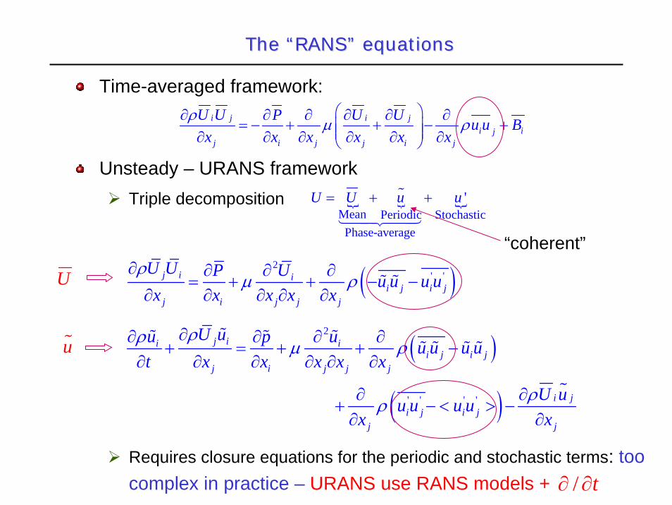
The The ““RANSRANS”” equationsequations

Time-averaged framework:

Unsteady – URANS frameworkTriple decomposition

Requires closure equations for the periodic and stochastic terms: too complex in practice – URANS use RANS models +

i j i ji ij

j i j j i j

U U P U U u u Bx x x x x x

ρ μ ρ⎛ ⎞∂ ∂ ∂ ∂ ∂ ∂

= − + + − +⎜ ⎟⎜ ⎟∂ ∂ ∂ ∂ ∂ ∂⎝ ⎠

{%{ {

Mean Periodic StochasticPhase-average

'U U u u= + +1442443

( )

( ) %

2

' ' ' '

j ii ii j i j

j i j j j

i ji j i j

j j

U uu up u u u ut x x x x x

U uu u u ux x

ρρ μ ρ

ρρ

∂∂ ∂∂ ∂+ = + + −

∂ ∂ ∂ ∂ ∂ ∂

∂ ∂+ − < > −∂ ∂

%% %%% % % %

( )2

' ' j i ii j i j

j i j j j

U U UP u u u ux x x x x

ρμ ρ

∂ ∂∂ ∂= + + − −

∂ ∂ ∂ ∂ ∂% %U

%u

“coherent”

/ t∂ ∂

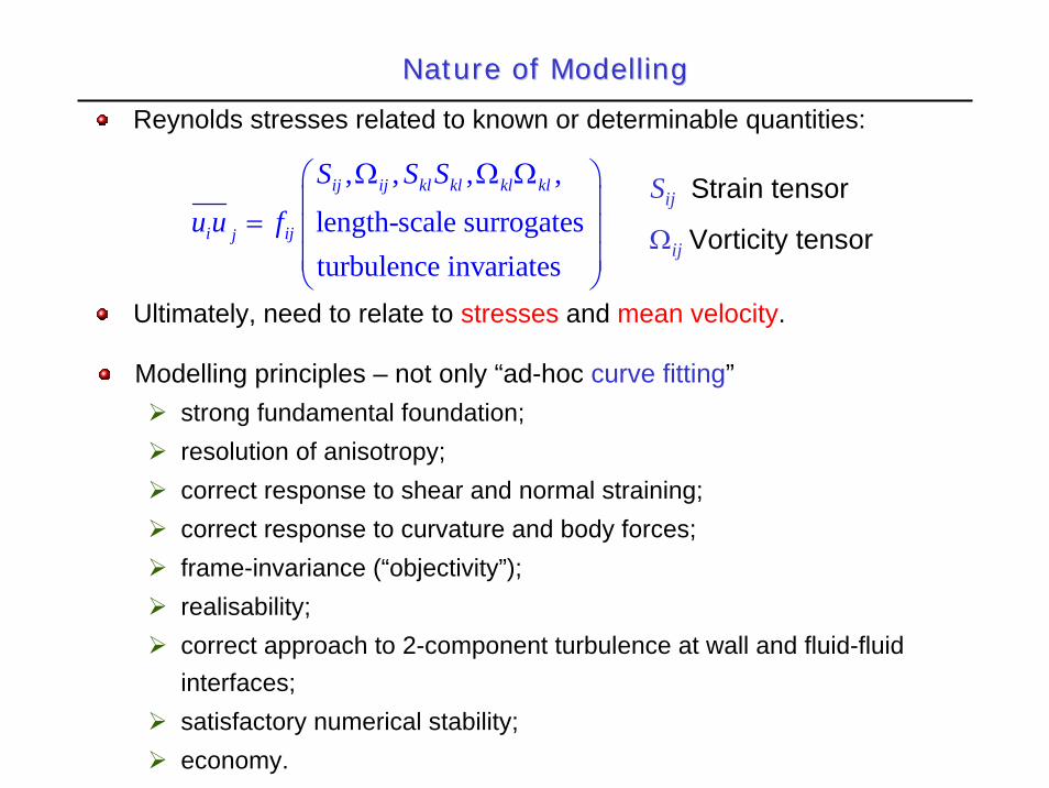
Reynolds stresses related to known or determinable quantities:

Ultimately, need to relate to stresses and mean velocity.

, , , , length-scale surrogatesturbulence invariates

ij ij kl kl kl kl

i ijj

S S Su u f

Ω Ω Ω⎛ ⎞⎜ ⎟

= ⎜ ⎟⎜ ⎟⎝ ⎠

Nature of ModellingNature of Modelling

Sij Strain tensor

Ωij Vorticity tensor

Modelling principles – not only “ad-hoc curve fitting”strong fundamental foundation;resolution of anisotropy; correct response to shear and normal straining;correct response to curvature and body forces;frame-invariance (“objectivity”);realisability;correct approach to 2-component turbulence at wall and fluid-fluid interfaces;satisfactory numerical stability;economy.

i ju u−

Model types Model types –– basic classificationbasic classification

Linear eddy viscosity models

Algebraic Differential (turbulence transport)

1-equation 2-equation

Non-linear eddy viscosity models

Second-moment closure (Reynolds-stress models)

“Algebraic” second-moment closure

Eddy-viscosity transport

Turbulence-energy transport

Turbulence energy + various length-scale surrogates

Wall-normal energy component + various length-scale surrogates

About 150 models & major variations, many meant for restricted flow classes

iuθ−

+ v2f

223i j t ij iju u S kν δ− = −

Linear EVM:Well suited to thin shear flowMuch less well suited to separated and highly 3d flowNo resolution of anisotropyWrong sensitivity to flow curvature, rotation, normal straining and body forcesReliant on ad-hoc corrections

Defects of linear eddyDefects of linear eddy--viscosity modelsviscosity models

Defects are rooted in Inapplicability of linear stress-strain relationsIsotropic nature of viscosity, relating to scalar turbulence propertiesCalibration by reference to simple, near-equilibrium flowsExcessive extrapolation to complex condition.

Only fundamentally credible alternativeModelling based on exact equations for the Reynolds stresses

Strong resistance from engineering community - complexity

ReynoldsReynolds--StressStress--Transport ModellingTransport Modelling

Introduce the Reynolds decomposition etc. into the NS equations.Subtract from this the corresponding RANS equation.Repeating the above, but with the indices i and j interchanged.Add the two equations.Time-averaging the result:

represent, respectively, stress convection, production by strain, production by body forces (e.g. buoyancy ), dissipation, pressure-strain redistribution and diffusion

ii iU U u= +

( ) 2

+ -

ijij ijij

ij

i j j ji ii k j k i j j i

k k k kFC P

j ji iik jki j k

j i k

Du u U uU u = u u + u u + f u + f u Dt x xx x

puu puup u u ux x x

ε

ν

νδ δρ ρ ρ

Φ

∂ ∂⎧ ⎫∂ ∂− −⎨ ⎬∂ ∂ ∂ ∂⎩ ⎭

⎛ ⎞∂∂ ∂+ − + +⎜ ⎟⎜ ⎟∂ ∂ ∂⎝ ⎠

1442443123 1424314444244443

1442443ij

i j

k

d

u ux

⎧ ⎫∂⎪ ⎪⎨ ⎬∂⎪ ⎪⎩ ⎭1444444442444444443

, , and , ,ij ij ij ij ij ijC P F dεΦ

Pressure-velocity

The Argument for resolving anisotropyThe Argument for resolving anisotropy

Production is a key process: it drives the stresses.

It requires no approximations if stresses and velocity are known

It is reasonable to assume, tentatively:

Stress = Production x Time (capital = interest rate x time)

Exact equations imply complex stress-strain linkage

Hence, simple EVM stress-strain linkage is inapplicable

Analogous linkage between scalar fluxes and production

Hence, Fourier-Fick law (eddy-diffusivity approximation)

not valid

-

ij

j ii i k j kj

k k

P

U Uu u u u + u u Body force production x x

ρ τ τ∂⎧ ⎫∂

←⎯→− + ×⎨ ⎬∂ ∂⎩ ⎭14444244443

-

ui

ii i k i

k k

P

Uu u u + u Body force production x x

ϕ

ϕ ϕρ ϕ τ ϕ τ⎧ ⎫∂Φ ∂←⎯→− + ×⎨ ⎬∂ ∂⎩ ⎭14444244443

ti

i

uxϕ

μρ ϕσ

∂Φ= −

∂

( )

( )

212

2 22

11

2

2

23

22

2 22

2 2

2 2 2

2

2 2

0

0

Duv p u v pu uvuvDt y x y y

Du p u uu vDt x y y

Dv p v pv vvDt y y y

Dw p w wvwDt z x

Uvy

Uuvy

μ ερ ρ ρ

μ ερ ρ

μ ερ ρ ρ

μρ ρ

⎛ ⎞⎛ ⎞∂ ∂ ∂ ∂= + + − + + −⎜ ⎟⎜ ⎟∂ ∂ ∂ ∂⎝ ⎠ ⎝ ⎠

∂ ∂ ∂= + − + −

∂ ∂ ∂

⎛ ⎞∂ ∂ ∂= + − + + −⎜ ⎟∂ ∂ ∂⎝

∂−

∂

⎠

∂ ∂

∂−

∂= + −

∂ ∂

∂

+∂ 33y

ε

⎫⎪⎪⎪⎪⎬⎪⎪⎪−⎪⎭

k equation= −∑

The equations for thin shear flowThe equations for thin shear flow

Only one shear strain, only one shear stress

0=∑ 2ε=∑Anisotropy

Anisotropy in simple shearAnisotropy in simple shear

Homogeneous shearDevelopment in time of stresses normalized by k

Strain rate x time

Channel flowNormal and shear stresses

22

22

22

2 2 2

2 ....

....

....

1 (2 ) .....2

Du UuDt x

Dv UvDt x

Dw UwDt x

Dk Uu v wDt x

∂= − +

∂

∂= +

∂

∂= +

∂∂

= − − − +∂

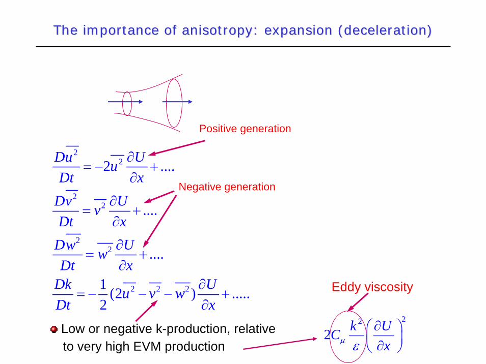
The importance of anisotropy: expansion (deceleration)The importance of anisotropy: expansion (deceleration)

Positive generation

Negative generation

Low or negative k-production, relative to very high EVM production

22

2 k UCxμ ε

∂⎛ ⎞⎜ ⎟∂⎝ ⎠

Eddy viscosity

Anisotropy in expansion and contractionAnisotropy in expansion and contraction

* / / 2ij ijS k S Sε=

23

i jij ij

u ua

kδ≡ −

Round impinging jetRound impinging jet

Wall-normal stress and mean velocity

Anisotropy in plain strainAnisotropy in plain strain

Other sensitivitiesOther sensitivities

Strong effect of curvature on anisotropyand shear stress.

Strong effects of rotation on anisotropyand shear stress

Inapplicability of Fourier-Fick law inscalar transport

Production of flux vector:

y

x

Vx

∂∂

x

y

P

S

i

iu i k i

k k

UP u u u x xφ ϕ∂Φ ∂

= − −∂ ∂

ReynoldsReynolds--StressStress--Transport ModellingTransport Modelling

Closure of exact stress-transport equations

Pressure-velocity, dissipation and diffusion require approximation

About 10-15 major closures forms

Modern closure aims at realisability, 2-component limit, coping with strong inhomogeneity and compressibility

Additional equations for dissipation tensor

At least 7 pde’s in 3D (up to 17 in heat/scalar transport)

Numerically difficult in complex geometries and flow

Can be costly

Dissipation and pressure-velocity are major sources of error

( )

ijij

i j j ii k j k

k kC AdvectiveTransport P Production

Du u U U = u u + u u Pressure velocityDt x x

Diffusion Dissipation

= =

∂⎧ ⎫∂− + −⎨ ⎬∂ ∂⎩ ⎭

+ −

123 14444244443

ijε

The exact dissipationThe exact dissipation--rate equationrate equation

1 2

"special" model fragments

ikl k l i j

k l j

UD k kC u u C u u CDt x x x kε ε εε ε εενδ

ε ε⎡ ⎤ ∂∂ ∂⎛ ⎞= + − −⎢ ⎥⎜ ⎟∂ ∂ ∂⎝ ⎠⎣ ⎦

+

%

In energy equilibrium, , and the imbalance is absorbs by

diffusion

Transport equations for are too complex as basis for modelling

Anisotropy in dissipation – algebraic approximations of the form:

In most models, reflecting assumption of small-scale isotropy

{ }1 2Production of( ) ( )Dissipation of C C fk

k kε ε εε

−

2 (1 )3

i jij e ij e

u uf f

kε εδ ε= + −

kP ε=

Modelled dissipationModelled dissipation--rate equationrate equation

Generalised gradient-diffusion approximation

ijε

1ef =

Closure Closure –– stress diffusionstress diffusion

Regarded as least influential (suggested by DNS/LES).

Represented as gradient-diffusion with tensorial diffusivity.

Simplest model:

Based on observation that the most important fragment in the exact diffusion term is .

It can be shown, via transport equations for triple correlation, , that the production of these triple correlations is by gradients of stresses of the form

Suggests (also on dimensional grounds)

j jij d k m

k m

u ukDiff c u ux xε

⎧ ⎫∂∂ ⎪ ⎪= − ⎨ ⎬∂ ∂⎪ ⎪⎩ ⎭

k i ju u u

k i ju u u

.....j j

ijk k mm

u uP u u

x

∂= − +

∂

{ }ijk(time scale) (production )ijk

Diff cx∂

= − ×∂

Closure Closure –– pressurepressure--strain / velocitystrain / velocity

Extremely important: responsible for redistribution among normalstresses. Regarded as the hardest term to modelPressure-velocity dictates energy transfer and hence But dictates

( )

( )

212

2 22

11

2

2

23

22

2 22

2 2

2 2 2

2

2 2

0

0

Duv p u v pu uvuvDt y x y y

Du p u uu vDt x y y

Dv p v pv vvDt y y y

Dw p w wvwDt z x

Uvy

Uuvy

μ ερ ρ ρ

μ ερ ρ

μ ερ ρ ρ

μρ ρ

⎛ ⎞⎛ ⎞∂ ∂ ∂ ∂= + + − + + −⎜ ⎟⎜ ⎟∂ ∂ ∂ ∂⎝ ⎠ ⎝ ⎠

∂ ∂ ∂= + − + −

∂ ∂ ∂

⎛ ⎞∂ ∂ ∂= + − + + −⎜ ⎟∂ ∂ ∂⎝

∂−

∂

⎠

∂ ∂

∂−

∂= + −

∂ ∂

∂

+∂ 33y

ε

⎫⎪⎪⎪⎪⎬⎪⎪⎪−⎪⎭

2v2v uv

Closure – pressure-strain

Subject to constrains:Isotropisation: transfer of energy from largest stress to lower ones

Inhibition of isotropisation at walls/interfaces (splatting, reflection)

shear stresses have to decline as isotropisation progresses

Guidance provided by ‘exact’ integration for pressure-fluctuations and substitution in pressure-velocity correlation

*2 *

*

* * *

*

1 ( ) = 4

1 ( 24

l

m

jiij

j i

jl m i

l m j iV

jm i

l j iV

U

uupx x

uu u

x

u dVx x x x

uu u dVx x x

ρ

π

π

⎛ ⎞∂∂Φ = +⎜ ⎟⎜ ⎟∂ ∂⎝ ⎠

⎧ ⎫⎛ ⎞∂⎛ ⎞∂ ∂⎪ ⎪+⎜ ⎟⎨ ⎬⎜ ⎟ ⎜ ⎟∂ ∂ ∂ ∂ −⎝ ⎠⎪ ⎪⎝ ⎠⎩ ⎭⎧ ⎫⎛ ⎞∂⎛ ⎞∂ ∂⎪ ⎪+ +⎜ ⎟⎨ ⎬⎜ ⎟ ⎜ ⎟∂ ∂ ∂ −⎝ ⎠⎪ ⎪⎝ ⎠⎩

⎛ ⎞∂⎜ ⎟

⎠ ⎭∂⎝

∫

∫

xx x

xx x

)

x

x*

V

+ body-force and surface terms

Aij

Bijkl

Suggests the general Ansatz:

Most complex model is cubic

Much more popular is the quasi-linear form

This is a sink term in the second-moment equations, depressing anisotropy in proportion to anisotropy of stresses and productions

Ensures that anisotropy in stresses and productions drives energy from above-average normal stresses to below-average ones

Coefficients sensitized to anisotropy invariants, turbulence Reynolds number…..in lieu of non-linear expansions

1 22 23 3

( body-force and wall terms)

ij i j ij ij ij ku u kC C P Pkε δ δ⎛ ⎞ ⎛ ⎞Φ = − − − −⎜ ⎟ ⎜ ⎟⎝ ⎠ ⎝ ⎠

+

2{ } { } 3

( body-force and wall terms)

i jkij ij ij ijkl ij ij ij

l

u uU = A a + k B a ax k

ε δ⎧ ⎫∂ ⎪ ⎪≡ −Φ ⎨ ⎬∂ ⎪ ⎪⎩ ⎭

+

Closure Closure –– pressurepressure--strainstrain

Closure Closure –– pressurepressure--strainstrain

Model PerformanceModel Performance

Construction and calibration rely heavily on highly-resolved experimental & simulation data

Done mostly by reference to thin-shear-flow data

Models work well for many flows

Notable exception: flow separating from curved surfaces (2d & 3d)

Associated with dynamics of highly unsteady separation (& pre-separation)

U-velocity close to wall

Separation from curved surfaceSeparation from curved surface

uv/Ub2

-0.04 -0.02 0 0.020

0.5

1

1.5

2

2.5

3

LS-AL-WJ-CLS-AJL-LES

(x/h=2.0)

εεωεω

uv/Ub2

-0.04 -0.02 0 0.02

LS-AL-WJ-CLS-AJL-LES

(x/h=6.0)

εεωεω

Shear-stress profiles with different models relative to LES

Model developmentsModel developments

Model defects are difficult to cure, but efforts are ongoing

Example: re-examination of dissipation and pressure-velocity interaction terms in separation from curved ramp

Foundation: highly-resolved simulation – near DNS, 25M nodes

ReH=13700; ReΘ = 1150

Second moments, invariants, budgets of all second moments….

Part of larger study on separation control with synthetic jets

Experimental data

Choice of basic model, based on full computation

Starting pointStarting point

LES: (x/h)s = 0.87 & (x/h)r=4.21

Shima: (x/h)s = 0.57 & (x/h)r=5.60 SSG+C: (x/h)s = 0.84/1.50 & (x/h)r=1.11/4.10

JH: (x/h)s = 0.79 & (x/h)r=4.15

Secondary recirculation

1.09

separation

Used to illustrate path to improvement

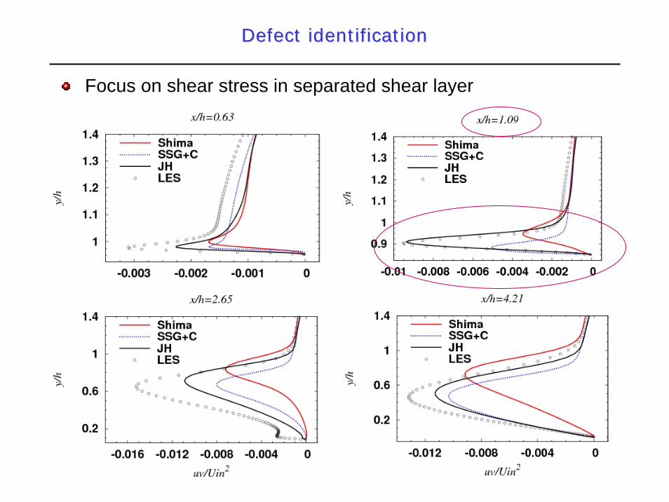
Focus on shear stress in separated shear layer

Defect identificationDefect identification

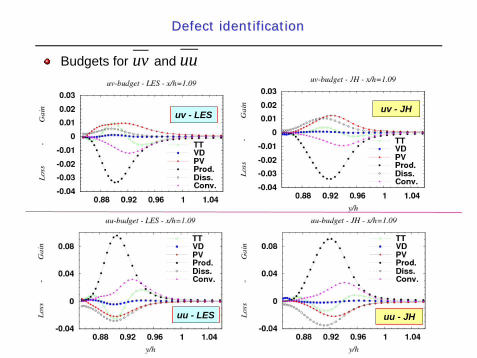
uv - LES

uu - LES

uv - JH

uu - JH

Defect identificationDefect identification

Budgets for and uuuv

A-priori study of dissipation-rate equationIsolated solution of equationLES strains and stresses input into equationOnly output is dissipationExamination of a range of corrections in efforts to procure agreement with LES data for dissipation rate

Model fragmentation Model fragmentation -- dissipationdissipation

Model fragmentation Model fragmentation -- dissipationdissipation

Ongoing efforts to sensitize dissipation to mean-flow/turbulence length scales

A-priori study of dissipation anisotropy – stresses and ε from LES into

Weighting function sensitized to anisotropy invariant

Use of anisotropy invariant

*

*

2(1 )3

( )312

ij s ij s ij

i i j k j i k k j k i j dj j lkij

p qp q d

f f

u u u u n n u u n n u u n n n n fu uk n n f

k

ε ε δ ε

εε

= + −

+ + +=

+1

1

(1 0.1Re )s

d t

f A

f

E−

= −

= +

2 3 2 3291 ( ) ; ; 8 3

i jij ij ij jk ki ij ij

u uA A A A a a A a a a a

kδ= − − = = = −

Various proposals

Model fragmentation Model fragmentation –– dissipation componentsdissipation components

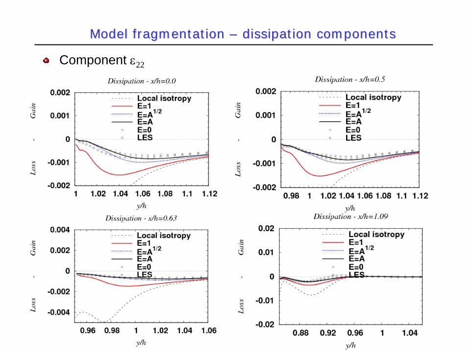
Component ε22

Model fragmentation Model fragmentation –– dissipation componentsdissipation components

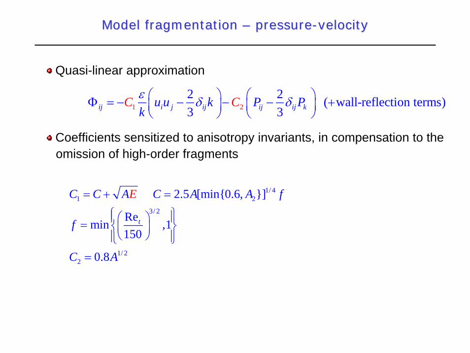
Model fragmentation Model fragmentation –– pressurepressure--velocityvelocity

1 22 2 ( wall-reflection terms)3 3ij i j ij ij ij ku u k P P

kC Cε δ δ⎛ ⎞ ⎛ ⎞Φ = − − − − +⎜ ⎟ ⎜ ⎟

⎝ ⎠ ⎝ ⎠

Quasi-linear approximation

Coefficients sensitized to anisotropy invariants, in compensation to theomission of high-order fragments

1/ 41 2

3/ 2

1/ 22

2.5 [min{0.6, }]

Remin ,1150

0.8

t

C C A C A A f

C A

E

f

= + =

⎧ ⎫⎪ ⎪⎛ ⎞= ⎨ ⎬⎜ ⎟⎝ ⎠⎪ ⎪⎩ ⎭

=

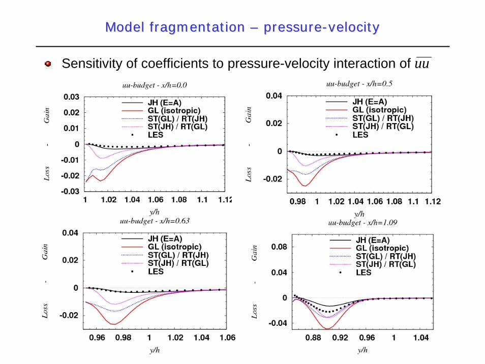
Sensitivity of coefficients to pressure-velocity interaction of uu

Model fragmentation Model fragmentation –– pressurepressure--velocityvelocity

General view and surface-pressure coefficient

ShockShock--induced Separation on 3D Jetinduced Separation on 3D Jet--AfterbodyAfterbody -- RSTMRSTM

ReL =2x107

0.5 M nodesCFL=O(1000)Desktop workstation, a few CPU hours

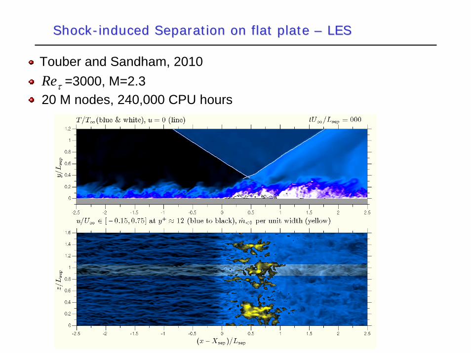
ShockShock--induced Separation on flat plate induced Separation on flat plate –– LESLES

Touber and Sandham, 2010Reτ =3000, M=2.320 M nodes, 240,000 CPU hours

Fundamentally, Second-moment closure is far superior to eddy-viscosity modelling.

In reality, closure is extremely challenging, because the anisotropy is an extremely influential model element and is difficult to approximate.

Redistribution and dissipation are especially influential.

Many ways of construction models, but all involve calibration.

Does involve “curve-fitting”, but is based on rational principles and physically tenable assumptions.

Little used, because of “the-simpler-the-better” attitude.

Second-moment closure is inappropriately complex in (most) thin shear flows, but the only fundamentally solid approach in complex strain.

Concluding remarksConcluding remarks