Single Object Tracking with TLD, Convolutional Networks, and AdaBoost

Albert Haque Fahim DalviComputer Science Department, Stanford University

{ahaque,fdalvi}@cs.stanford.edu

AbstractWe evaluate the performance of the TLD algorithm using

AdaBoost and SVMs with HOG, CNN, and raw features.We improve runtime performance through algorithmic andimplementation optimizations and are able to achieve near-realtime frame rates of over 10 FPS for selected videos. OurSVM-HOG implementation achieves an average overlap of54% and 60%, and an average MAP of 67% and 66%, onthe validation and test set, respectively.

1. Introduction & Related WorkObject tracking often uses object detection (i.e. track-

ing by detection) and requires an appropriate appearancemodel to localize the object. Static appearance models usethe first frame or require offline generation. In [26], the au-thors combine SIFT features with mean shift [7] for objectsegmentation, detection, and tracking. In [2], Babaeian etal. also use mean shift but instead use a collection of vari-ous visual features for tracking. However, since both [26, 2]construct an appearance model from the first frame, theyoften fail when the object’s appearance changes over time(e.g. illumination, scale, and orientation changes). Possiblesolutions are to use features invariant to these transforma-tions or to employ adaptive appearance models.

Adaptive appearance models adjust over time to accom-modate object transformations throughout the video. Theauthors in [11] divide their appearance model into threecomponents: a stable long time-course component, a 2-frame transient component, and an outlier set. Each compo-nent is assigned a dynamic weight over time which providesadditional robustness and improves tracking performance.In [6], Collins et al. attempt to select appropriate features inan online manner. In [3], Babenko et al. employ a multipleinstance learning model that bootstraps itself by using pos-itive and negative examples from the current tracker stateand current frame. They convert MILBoost [25] into an on-line algorithm by updating all weak classifiers using bags ofexamples drawn from the current frame.

In-class presentation: https://youtu.be/RrvWuKVYOBg. Re-fer to this paper for authoritative results.

Attempts at fusing both tracking and detection tech-niques have proven successful in the past. In [15], theauthors use a tracking, learning, and detection framework,which we describe in greater detail in Section 2. Since thedetector and tracker have different objectives, namely, thedetector generates labels while the tracker estimates loca-tion, these objectives may not be properly aligned. In [9],Hare et al. propose a kernelized, structured-output SVM tobetter integrate the object detection objective with the track-ing objective.

The methods described thus far are concerned with sin-gle object tracking. Adaptive appearance models can be ap-plied to multi-object tracking as well. In [19], Pirsiavashet al. employ an iterative graph-based solution for multi-object tracking with a single camera using network flows.Edge weights are assigned by an appearance model. A pop-ular research area which builds on single-camera problemsis multi-camera multi-object tracking [10, 16], often usingcameras with overlapping field of views.

2. TLD AlgorithmIn [15], Kalal et al. investigate long term-tracking by de-

composing the task into tracking, learning, and detectioncomponents. In this section, we review each component.

Tracker. The tracker estimates the object’s motion be-tween frames under assumption that the object is visible.The method proposed by Kalal et al. uses (i) the Lucas-Kanade tracker [17], which formulates the tracking problema least squares optimization using optical flow, and (ii) usesthe Median-Flow tracker [14]. This method works well, ex-cept a problem arises when the object movies outside thefield of view or is occluded in the scene. It will be difficultfor the tracker to recover since it has lost the object’s cur-rent motion information. To remedy this, a detection step isincluded to prevent complete TLD failure.

Detector. The goal of the detection component is to lo-calize the object in the frame. This step runs independentlyfrom the tracker and is implemented by Kalal et al. as athree-stage cascade model. Given all possible boundingboxes in the image, first, a patch variance filter is appliedto eliminate patches that are not similar to the object (e.g.

1

Table 1. Performance of patch features using a SVM. Average metrics are shown. Standard deviations are across images..Validation Set (n = 4) Test Set (n = 5)

Feature Overlap AUC MAP Overlap AUC MAPCNN 37.0± 27.0 38.1± 25.9 30.4± 46.9 33.9± 11.6 35.0± 10.0 14.2± 9.7HOG 54.6± 32.9 55.6± 31.2 67.4± 52.3 60.4± 15.4 60.4± 15.4 66.8± 36.3Raw 65.3± 21.5 65.7± 20.8 75.7± 42.0 44.5± 27.9 45.7± 26.7 49.1± 44.1

Table 2. Performance of learning algorithms using HOG features. Average metrics are shown. Standard deviations are across images.Validation Set (n = 4) Test Set (n = 5)

Learning Algorithm Overlap AUC MAP Overlap AUC MAPAdaBoost 55.2± 25.2 55.7± 24.4 67.2± 51.3 55.0± 22.4 55.6± 21.2 61.9± 38.0SVM 54.6± 32.3 55.6± 31.2 67.4± 52.3 60.4± 15.4 60.4± 15.4 66.8± 36.3

background sky or grass). Second, an ensemble classifierassigns a label to each bounding box using random ferns.Third, a nearest neighbor classifier compares the remain-ing candidate bounding boxes with positives from previousframes. As the object moves throughout the video, we mustupdate each step of the cascaded classifier.

Learning. To update the appearance model, Kalal et al.propose a P-expert and N-expert [15, 13]. The goal of theP-expert is to identify new, reliable appearances of the ob-ject and update the detector accordingly. Reliable is de-fined as an appearance that agrees with both the detector andtracker (defined by thresholds). These reliable appearancesare then augmented and used to update the detection model.The goal of the N-expert is to identify the background. In amanner similar to the P-expert, the N-expert augments neg-ative training examples if both the detector and tracker areconfident about a bounding box.

3. Technical ApproachIn this section, we describe our motivation and algorith-

mic modifications to the original TLD paper [15]. We de-scribe our feature representations, data augmentation strat-egy, learning methods, bounding box priors, and integrator.

3.1. Features

As a baseline, we use raw pixels as the feature represen-tation. We transform the pixel values to have zero mean andunit variance. All image patches are resized to 25x25 beforemean centering, resulting in 625 features per patch.

HOG features capture local object appearance and shapebetter than raw pixels. For this reason, we evaluate HOGfeatures as well. Before extracting HOG features, we resizeeach patch to 25x25. Nine bins are used for each block ofsize 8x8 pixels. This results in 144 features.

To capture higher level patch and color (or grayscale)representations, we use a CNN as a feature extractor. Weuse the VGG-16 network architecture [21] pre-trained onImageNet [20] and extract features from the non-rectifiedfully-connected layer (fc7). This results in 4096 features.

Table 1 shows the performance of these features whenusing a SVM. Across the entire dataset (9 videos), HOGachieves an average overlap and MAP of 58% and 67%,

respectively, whereas raw pixels achieve 51% and 58%, re-spectively. Unfortunately, the CNN does not perform well.Based on these results, we use HOG as our primary featurerepresentation. We discuss these results in more detail inSection 5.

3.2. Data Augmentation

Certain videos undergo dramatic illumination changes(e.g. Human8, Man) while some videos show the objectat varying scales (e.g. Vase). To combat this, we performmore extreme warps. For the initial frame, we rotate pos-itive examples by up to ±30◦ and scale by up to ±10%.During the update phase, we rotate positive examples by upto ±20◦ and also scale up to ±10%. These parameters weretuned based on performance on difficult video sequences(e.g. Bolt2, Vase, Human8, Man) to adapt to illuminationand scale changes without compromising performance onvideos without many transformations (e.g. Deer, Car4).

3.3. Learning Algorithms

The original TLD paper proposes an ensemble of fernclassifiers [4] as part of their casaded classifier. Instead of afern classifier, we use a SVM. To avoid completely deviat-ing from the original TLD paper, we also experiment withan ensemble classifier: AdaBoost.

SVMs have been used for object tracking in the past[1, 22, 18]. Similar to [27], we use an SVM with a Gaussiankernel to classify false and positive object examples. Boost-ing algorithms leverage an ensemble of base classifiers toimprove overall classification performance. AdaBoost, inparticular, attempts to find an accurate classifier in an inter-ative manner by constructing a distribution of weights foreach base classifier proportional to each base classifier’s er-ror on the training set. Since AdaBoost has been successfulat various computer vision tasks (e.g. face detection [23],pedestrian detection [24], and online tracking [8]), we de-cide to evaluate its performance in our study.

Our ensemble consists of 50 weak threshold classifiers.Each weak classifier attempts to divide the training datainto two classes by finding the best threshold for each fea-ture. The number of weak classifiers was selected to balancetraining time, overfitting, and performance.

2

Table 2 shows the performance of both learning algo-rithms. Computed across all 9 videos, AdaBoost achievesan average overlap and MAP of 55% and 63%, respectivelywhile the SVM achieves 58% and 67%, respectively. Basedon these results, we use SVM+HOG as our final learningalgorithm. Results are further discussed in Section 5.

3.4. Bounding Box Priors

We introduce three priors: (i) bounding box location, (ii)bounding box size, and (iii) long term memory. Our goalis two-fold. First, we wish to decrease algorithm runtimeby decreasing the number of bounding boxes sent to later-stage processing steps. Second, we wish to improve trackerperformance by eliminating bounding boxes that do not fitwith our prior knowledge of the object.

Location. Due to the frame rate of the original video,we know that the object being tracked cannot dramati-cally change position between two frames. We introducea bounding box location delta denoted by δL. The center ofa bounding box at time t + 1 must be within δL from thecenter of the bounding box at time t in both the x and ydimensions. We set this value to 30 pixels.

Size. Similar to the bounding box location prior, we in-troduce a prior on the bounding box size. We know thatthe object cannot abruptly change in size between frames.We introduce a bounding box size delta to enforce this con-straint. We set this value to δS = 20 pixels. This value wasselected by empirical testing.

Long Term Memory. The bounding box for frame 1is the ground truth and should therefore carry more weightduring detection in later frames. To do so, we introduce thenotion of long term memory. The original TLD paper sug-gests random forgetting of old examples during the updatestage of the nearest neighbor classifier. We continue to ran-domly forget examples but also require the algorithm to re-member some positive and negative examples from the firstframe. This is primarily meant to combat “drift” when thealgorithm begins to generate incorrect positive examples.We set long term memory to 200 examples. For reference,our nearest neighbor classifier remembers 1000 examples.Care must be taken to not saturate the history with the ap-pearance from the first frame. It is possible the true objectappearance in later frames differs from the first frame.

3.5. Integrator

We use the standard TLD integrator implementation withone modification: if the tracker is not defined but the de-tector is, we always reinitialize the tracker. Previously, thetracker would only be reinitialized if the detector resulted ina single clustering. For Bolt2 (SVM-Raw), this resulted inan average overlap and MAP of 26.3% and 26.9%, respec-tively. If multiple detected clusters exist, we reinitialize thetracker from the bounding box cluster with the highest con-

fidence. For Bolt2, we saw a large improvement in MAP –average overlap and MAP increased to 40.5% and 27.2%,respectively. We saw similar gains for videos where thebounding box is lost at least once (e.g. Bolt2, Deer).

4. Code DetailsExecution. All commands must be run from inside

the code/ folder (and not inside one of its subfolders).To view the help message, run the following command:main(). Inputs must be entered in argument-value pairs.Below is an example command to run the program:

main(’video’,’Dancer2’,’feature’,’raw’,’classifier’,’svm’)

An optional argument is num frames to track whichdefaults to Inf if not specified. Table 3 shows the list of ar-guments and acceptable values. The video is case sensitivewhereas the feature and classifier are not.

Table 3. List of main() arguments and acceptable values.Argument Name Required? Acceptable Valuesvideo Yes Any input video namefeature Yes raw, hog, cnn, rawhog, allclassisifer Yes svm, adaboostnum frames to track No Integer value

Extensions. Our extensions are located in the ex-tensions folder. We used an open source implementa-tion of AdaBoost located in adaboost.m and borrowedsome lines of code from Caffe’s Matlab implementation inextractCNN.m. Each file contains a link to the originalonline source.

Dependencies. For HOG feature extraction, the Mat-lab Computer Vision toolbox must be installed. To runCNN feature extraction, Caffe’s Matlab implementationmust be installed (also known as MatCaffe). The ap-propriate mex file (typically caffe.mexa64 located inCAFFE ROOT/matlab/caffe) must be copied to ourcode/caffe/ folder. Additionally, the VGG-16 networkmodel must be present in our code/caffe/models/folder.

5. ExperimentsWe use the Caffe [12] and cuDNN [5] libraries for our

convolutional network implementation. All experimentswere performed on one workstation equipped with a hex-core Intel 4930K CPU with 32 GiB of main memory. Asingle GTX Titan X with 12 GiB of memory was used forGPU computations.

5.1. Discussion

First we discuss the results for the different features andthen move to a discussion about the learning algorithms. Ta-ble 1 shows the results of each feature when using a SVM

3

. . .

. . .

Frame 5 Frame 6 Frame 7 Frame 8 Frame 9 Frame 128

SVM-HOG

SVM-Raw

SVM-CNN

. . .

Figure 1. Comparison of HOG, raw, and CNN features for the SVM. HOG features successfully track the object from frame 6 to 7 due toHOG’s strength at capturing shape instead of color. Even with data augmentation (warping), raw pixels are unable to track the object.

Frame 2 Frame 3 Frame 4 Frame 5 Frame 6 Frame 7

SVM-HOG

SVM-Raw

Figure 2. Video of a successful tracking result. Both HOG and raw pixels are able to track the car. Although the car undergoes illuminationchanges, raw pixels are able to detect the object due to our data augmentation and relatively small illumination change.

classifier. We can see that HOG outperforms both Raw andCNN, on average. Moving to a qualitative discussion, weanalyze Human8 in Figure 1. As previously mentioned,SVM-HOG (first row) is able to successfully track the ob-ject from frame 6 to 7 due to it’s shape modeling ability. Theillumination change causes raw pixels to fail. CNN featuresare able to track the object for the first 30 frames but areunable to follow the object to frame 128. One possible ex-planation is overfitting. Our CNN feature vector consists of4096 features but our positive and negative history consistsof 2000 total examples. A future experiment could increasethe number of training examples in the history to provide asufficient number of training examples for our SVM.

AdaBoost performs similarly to SVM on the validationset (Table 2). However, on the test set, AdaBoost’s per-formance deteriorates. For the Jumping video, SVM-HOGgenerates roughly 20-30 bounding boxes after the nearestneighbor step. AdaBoost-HOG, however, generates around80 boxes per frame. This could lead to a higher number offalse positives which cause AdaBoost to select the incorrectbox. It may be beneficial to increase the nearest neighborthresholds for AdaBoost to reduce the number of boxes. Ta-bles 5 and 6 list performance metrics for each video.

Figure 2 shows our SVM-HOG method working well onthe car video. As expected, it successfully models changein illumination as the car passes under the tree in frames 2to 6. For comparison, SVM-Raw also does well on Car4.

5.2. Runtime Performance & Optimizations

To achieve higher frame rates, we optimize both the codeand the original TLD algorithm. First, we employ our ownmethod for patch resizing. Matlab’s imresize implemen-tation requires 2 ms per patch. Since our features requirefixed image sizes, this introduces an overhead of severalseconds per frame. Our implementation subsamples eachpatch without interpolation and results in 0.2 ms per patch.

Second, we change the order of which the bounding boxfilters are applied. The original TLD algorithm performs thevariance filter as the first step. This requires each patch to beextracted from the image, from which the variance is com-puted. Since this is the first step, all patches are extractedand computed on. Because we introduce bounding box pri-ors, we can efficiently reduce the set of candidate boundingboxes before the variance is computed. Our bounding boxpriors allow us to reduce the number of inputs into the vari-ance stage by an order of magnitude.

4

SVM-HOG

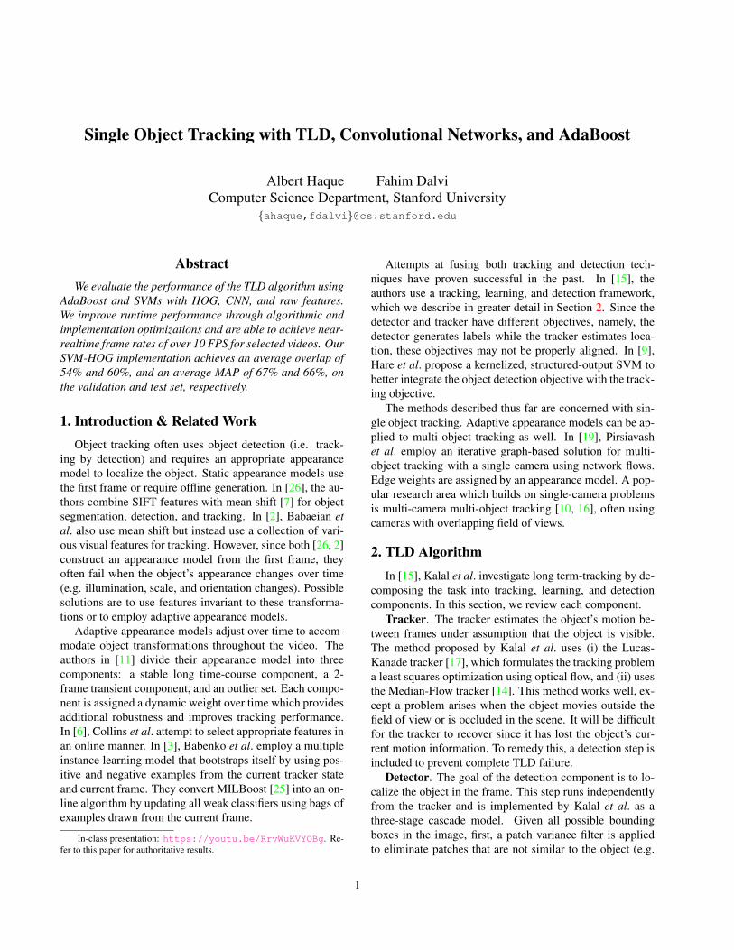
Frame 42 Frame 43 Frame 44 Frame 45 Frame 46

Figure 3. Error analysis on the Bolt2 video. When moving from frame 43 to 44, our model is confused and selects the objects behind therunners. This can be attributed to HOG features not capturing the color information.

Frame 71 Frame 72 Frame 73 Frame 74 Frame 75 Frame 76

SVM-HOG

Figure 4. Error analysis on the Vase video. Because the vase rapidly changes in size, our tracker is unable to correctly resize the boundingbox. This could be attributed to insufficient data augmentation or too strict of a bounding box size delta.

Bol

t2Car

4

Dan

cer2

Dee

rFis

h

Hum

an8

Jum

ping

Man

Vas

e0

2

4

6

8

10

12

14Frames per second using a SVM

Fra

mes

per

sec

ond

CNNHOGRaw

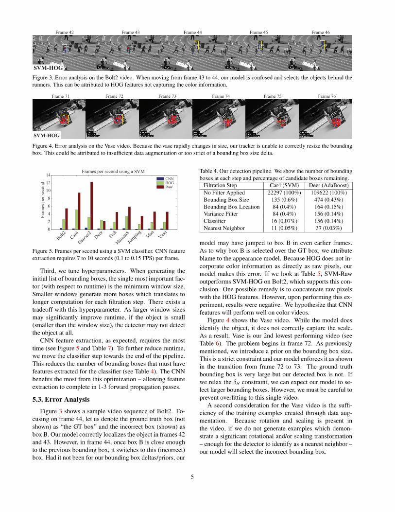
Figure 5. Frames per second using a SVM classifier. CNN featureextraction requires 7 to 10 seconds (0.1 to 0.15 FPS) per frame.

Third, we tune hyperparameters. When generating theinitial list of bounding boxes, the single most important fac-tor (with respect to runtime) is the minimum window size.Smaller windows generate more boxes which translates tolonger computation for each filtration step. There exists atradeoff with this hyperparameter. As larger window sizesmay significantly improve runtime, if the object is small(smaller than the window size), the detector may not detectthe object at all.

CNN feature extraction, as expected, requires the mosttime (see Figure 5 and Table 7). To further reduce runtime,we move the classifier step towards the end of the pipeline.This reduces the number of bounding boxes that must havefeatures extracted for the classifier (see Table 4). The CNNbenefits the most from this optimization – allowing featureextraction to complete in 1-3 forward propagation passes.

5.3. Error Analysis

Figure 3 shows a sample video sequence of Bolt2. Fo-cusing on frame 44, let us denote the ground truth box (notshown) as “the GT box” and the incorrect box (shown) asbox B. Our model correctly localizes the object in frames 42and 43. However, in frame 44, once box B is close enoughto the previous bounding box, it switches to this (incorrect)box. Had it not been for our bounding box deltas/priors, our

Table 4. Our detection pipeline. We show the number of boundingboxes at each step and percentage of candidate boxes remaining.

Filtration Step Car4 (SVM) Deer (AdaBoost)No Filter Applied 22297 (100%) 109622 (100%)Bounding Box Size 135 (0.6%) 474 (0.43%)Bounding Box Location 84 (0.4%) 164 (0.15%)Variance Filter 84 (0.4%) 156 (0.14%)Classifier 16 (0.07%) 156 (0.14%)Nearest Neighbor 11 (0.05%) 37 (0.03%)

model may have jumped to box B in even earlier frames.As to why box B is selected over the GT box, we attributeblame to the appearance model. Because HOG does not in-corporate color information as directly as raw pixels, ourmodel makes this error. If we look at Table 5, SVM-Rawoutperforms SVM-HOG on Bolt2, which supports this con-clusion. One possible remedy is to concatenate raw pixelswith the HOG features. However, upon performing this ex-periment, results were negative. We hypothesize that CNNfeatures will perform well on color videos.

Figure 4 shows the Vase video. While the model doesidentify the object, it does not correctly capture the scale.As a result, Vase is our 2nd lowest performing video (seeTable 6). The problem begins in frame 72. As previouslymentioned, we introduce a prior on the bounding box size.This is a strict constraint and our model enforces it as shownin the transition from frame 72 to 73. The ground truthbounding box is very large but our detected box is not. Ifwe relax the δS constraint, we can expect our model to se-lect larger bounding boxes. However, we must be careful toprevent overfitting to this single video.

A second consideration for the Vase video is the suffi-ciency of the training examples created through data aug-mentation. Because rotation and scaling is present inthe video, if we do not generate examples which demon-strate a significant rotational and/or scaling transformation– enough for the detector to identify as a nearest neighbor –our model will select the incorrect bounding box.

5

Table 5. Detailed validation set results. Overlap is denoted as OLP.Bolt2 Car4 Dancer2 Deer Average

Model OLP AUC MAP OLP AUC MAP OLP AUC MAP OLP AUC MAP OLP AUC MAPSVM-CNN 15.8 19.1 2.1 27.7 27.7 4.5 67.5 67.7 84.6 41.4 41.6 13.7 37.0 38.1 30.4SVM-HOG 17.2 20.4 7.1 79.5 79.8 96.1 67.2 66.9 99.3 69.3 68.9 94.4 54.6 55.6 67.4SVM-Raw 40.5 41.7 27.2 77.7 77.8 100.0 78.0 77.7 100.0 63.5 64.0 86.7 65.3 65.7 75.7AdaBoost-CNN 39.2 39.5 12.8 14.8 14.5 1.0 68.7 68.8 95.7 29.6 29.8 9.2 40.9 40.0 36.5AdaBoost-HOG 26.2 27.7 8.0 72.5 72.4 96.9 67.0 67.1 97.0 68.8 68.5 92.4 55.2 55.7 67.28AdaBoost-Raw 38.5 39.6 24.6 76.9 76.8 100.0 75.5 75.0 98.2 70.9 70.5 91.4 63.3 63.7 74.2

Table 6. Detailed test set results. Overlap is denoted as OLP.Fish Human8 Jumping Man Vase Average

Model OLP AUC MAP OLP AUC MAP OLP AUC MAP OLP AUC MAP OLP AUC MAP OLP AUC MAPSVM-CNN 39.6 40.0 11.5 18.5 22.0 19.2 50.4 50.3 29.3 19.4 23.5 20.4 34.1 34.0 2.7 33.8 35.2 16.1SVM-HOG 45.8 45.7 34.8 61.4 61.9 65.2 70.3 70.0 96.0 77.8 78.1 98.3 37.9 37.9 12.2 60.4 60.4 66.8SVM-Raw 29.8 31.2 13.3 4.8 9.4 2.4 62.2 62.2 79.8 78.8 79.3 100.0 28.3 28.3 12.5 44.5 45.7 49.1AdaBoost-CNN 18.1 18.4 7.1 14.6 17.9 10.0 41.4 41.5 10.4 19.4 23.5 20.4 30.0 29.9 2.6 22.5 26.8 9.9AdaBoost-HOG 61.2 60.9 59.8 18.2 22.0 19.6 67.3 67.3 91.8 77.0 77.4 96.0 37.9 37.9 12.2 55.0 55.6 61.9AdaBoost-Raw 21.0 23.3 9.3 3.5 8.1 2.3 60.7 60.9 81.4 60.7 60.9 81.5 23.3 22.9 14.9 39.9 41.1 46.7

Table 7. Algorithm runtime in frames processed per second (FPS). Higher is better.Model Bolt2 Car4 Dancer2 Deer Fish Human8 Jumping Man VaseSVM-CNN 0.22 0.03 0.22 0.10 0.11 0.14 0.06 0.10 0.11SVM-HOG 1.56 3.57 2.88 1.68 1.81 2.39 0.88 1.11 1.36SVM-Raw 4.90 8.92 11.80 1.64 3.98 5.51 2.99 4.14 4.02AdaBoost-CNN 0.14 0.21 0.21 0.13 0.10 0.15 0.07 0.10 0.1AdaBoost-HOG 1.12 1.56 0.34 0.74 0.14 1.05 0.49 0.77 0.63AdaBoost-Raw 0.50 0.57 0.46 0.50 0.52 0.37 0.47 0.45 0.51

References[1] S. Avidan. Support vector tracking. PAMI, 2004. 2[2] A. Babaeian, S. Rastegar, M. Bandarabadi, and M. Rezaei.

Mean shift-based object tracking with multiple features. InSoutheastern Symposium on System Theory, 2009. 1

[3] B. Babenko, M.-H. Yang, and S. Belongie. Visual trackingwith online multiple instance learning. In CVPR, 2009. 1

[4] A. Bosch, A. Zisserman, and X. Muoz. Image classificationusing random forests and ferns. In ICCV, 2007. 2

[5] S. Chetlur, C. Woolley, P. Vandermersch, J. Cohen, J. Tran,B. Catanzaro, and E. Shelhamer. cudnn: Efficient primitivesfor deep learning. arXiv, 2014. 3

[6] R. T. Collins, Y. Liu, and M. Leordeanu. Online selection ofdiscriminative tracking features. PAMI, 2005. 1

[7] D. Comaniciu and P. Meer. Mean shift: A robust approachtoward feature space analysis. PAMI, 2002. 1

[8] H. Grabner, M. Grabner, and H. Bischof. Real-time trackingvia on-line boosting. In BMVC, 2006. 2

[9] S. Hare, A. Saffari, and P. H. Torr. Struck: Structured outputtracking with kernels. In ICCV, 2011. 1

[10] O. Javed, Z. Rasheed, and K. Shafique. Tracking across mul-tiple cameras with disjoint views. In ICCV, 2003. 1

[11] A. D. Jepson, D. J. Fleet, and T. F. El-Maraghi. Robust onlineappearance models for visual tracking. PAMI, 2003. 1

[12] Y. Jia, E. Shelhamer, J. Donahue, S. Karayev, J. Long, R. Gir-shick, S. Guadarrama, and T. Darrell. Caffe: Convolutionalarchitecture for fast feature embedding. arXiv, 2014. 3

[13] Z. Kalal, J. Matas, and K. Mikolajczyk. Online learning ofrobust object detectors during unstable tracking. In ICCVWorkshops, 2009. 2

[14] Z. Kalal, K. Mikolajczyk, and J. Matas. Forward-backwarderror: Automatic detection of tracking failures. In ICPR,2010. 1

[15] Z. Kalal, K. Mikolajczyk, and J. Matas. Tracking-learning-detection. PAMI, 2012. 1, 2

[16] S. Khan and M. Shah. Consistent labeling of tracked objectsin multiple cameras with overlapping fields of view. PAMI,2003. 1

[17] B. D. Lucas, T. Kanade, et al. An iterative image registra-tion technique with an application to stereo vision. In IJCAI,1981. 1

[18] C. P. Papageorgiou, M. Oren, and T. Poggio. A generalframework for object detection. In ICCV. IEEE, 1998. 2

[19] H. Pirsiavash, D. Ramanan, and C. C. Fowlkes. Globally-optimal greedy algorithms for tracking a variable number ofobjects. In CVPR, 2011. 1

[20] O. Russakovsky, J. Deng, H. Su, J. Krause, S. Satheesh,S. Ma, Z. Huang, A. Karpathy, A. Khosla, M. Bernstein,A. C. Berg, and L. Fei-Fei. Imagenet large scale visual recog-nition challenge. IJCV, 2015. 2

[21] K. Simonyan and A. Zisserman. Very deep convolutionalnetworks for large-scale image recognition. arXiv, 2014. 2

[22] F. Tang, S. Brennan, Q. Zhao, and H. Tao. Co-tracking usingsemi-supervised support vector machines. In ICCV, 2007. 2

[23] P. Viola and M. Jones. Rapid object detection using a boostedcascade of simple features. In CVPR, 2001. 2

[24] P. Viola, M. J. Jones, and D. Snow. Detecting pedestriansusing patterns of motion and appearance. In ICCV, 2003. 2

[25] C. Zhang, J. C. Platt, and P. A. Viola. Multiple instanceboosting for object detection. In NIPS, 2005. 1

[26] H. Zhou, Y. Yuan, and C. Shi. Object tracking using siftfeatures and mean shift. Computer vision and image under-standing, 2009. 1

[27] W. Zhu, S. Wang, R.-S. Lin, and S. Levinson. Tracking ofobject with svm regression. In CVPR, 2001. 2

6