SINGLE DISH EXPOSURE TIME CALCULATOR User Manual · SINGLE DISH EXPOSURE TIME CALCULATOR User Manual Release 1.0 A. Zanichelli 1, S. Righini , K.-H. Mack 1, A. Orfei , V. Vacca2 in

.

SINGLE DISH EXPOSURE TIME CALCULATOR

User Manual

Release 1.0

A. Zanichelli1, S. Righini1, K.-H. Mack1, A. Orfei1, V. Vacca2

in collaboration with the SRT Astrophysical Validation Team∗

INAF - Istituto di RadioastronomiaReport no. 487/15

Referee: M. Giroletti1

∗ The SRT Astrophysical Validation Team:Matteo Bachetti3, Marco Bartolini1, Pietro Bolli4, Marta Burgay3, Marco Buttu3, Ettore Carretti3, PaolaCastangia3, Silvia Casu3, Gianni Comoretto4, Raimondo Concu3, Alessandro Corongiu3, Nicolo D’Amico5,Elise Egron3, Antonietta Fara3, Francesco Gaudiomonte3, Federica Govoni3, Daria Guidetti1, Maria NoemiIacolina3, Francesca Loi3, Fabrizio Massi4, Andrea Melis3, Carlo Migoni3, Matteo Murgia3, Francesco Nasyr3,Alessandro Orfei1, Andrea Orlati1, Alberto Pellizzoni3, Delphine Perrodin3, Tonino Pisanu3, Sergio Poppi3, Is-abella Prandoni1, Roberto Ricci1, Alessandro Ridolfi3, Simona Righini1, Ignazio Porceddu3, Carlo Stanghellini1,Andrea Tarchi3, Caterina Tiburzi3, Alessio Trois3, Valentina Vacca2, Giuseppe Valente3, Alessandra Zanichelli1,

1 INAF - Istituto di Radioastronomia, via P.Gobetti 101, 40129 Bologna, Italy.2 MPA, Garching, Germany.3 INAF - Osservatorio Astronomico di Cagliari, Via della Scienza 5, 09047 Selargius (CA), Italy.4 INAF - Osservatorio Astrofisico di Arcetri, Largo Enrico Fermi 5, I-50125, Firenze, Italy.5 Dipartimento di Matematica e Informatica, Universita degli Studi di Cagliari, Palazzo delle Scienze, ViaOspedale 72, 09124 Cagliari, Italy.

Acknowledgements: the authors would like to thank Franco Buffa (Osservatorio Astronomico di Cagliari) forhaving kindly provided us useful meteorological information for the SRT site.

1

Contents

1 Introduction 3

2 ETC Overview 3

3 Basic Formulae 53.1 Bandwidth . . . . . . . . . . . . . . . . . . . . . . . . . . . . . . . . . . . . . . . . . . . . . . . . 53.2 System Temperature . . . . . . . . . . . . . . . . . . . . . . . . . . . . . . . . . . . . . . . . . . . 63.3 Receiver Gain . . . . . . . . . . . . . . . . . . . . . . . . . . . . . . . . . . . . . . . . . . . . . . . 6

4 Radiometer Formula + Position Switching Computations 64.1 Input Parameters . . . . . . . . . . . . . . . . . . . . . . . . . . . . . . . . . . . . . . . . . . . . . 74.2 Computations: given σTOT evaluate tTOT . . . . . . . . . . . . . . . . . . . . . . . . . . . . . . . 74.3 Computations: given tTOT evaluate σTOT . . . . . . . . . . . . . . . . . . . . . . . . . . . . . . . 74.4 Position Switching computations . . . . . . . . . . . . . . . . . . . . . . . . . . . . . . . . . . . . 74.5 Output Parameters . . . . . . . . . . . . . . . . . . . . . . . . . . . . . . . . . . . . . . . . . . . . 8

5 On-The-Fly Cross Scan computations 85.1 Input Parameters . . . . . . . . . . . . . . . . . . . . . . . . . . . . . . . . . . . . . . . . . . . . . 85.2 Computations: given σTOT evaluate tTOT . . . . . . . . . . . . . . . . . . . . . . . . . . . . . . . 95.3 Computations: given tTOT evaluate σTOT . . . . . . . . . . . . . . . . . . . . . . . . . . . . . . . 115.4 Output Parameters . . . . . . . . . . . . . . . . . . . . . . . . . . . . . . . . . . . . . . . . . . . . 11

6 On-The-Fly Map computations 126.1 Input Parameters . . . . . . . . . . . . . . . . . . . . . . . . . . . . . . . . . . . . . . . . . . . . . 126.2 Computations: given σTOT evaluate tTOT . . . . . . . . . . . . . . . . . . . . . . . . . . . . . . . 136.3 Computations: given tTOT evaluate σTOT . . . . . . . . . . . . . . . . . . . . . . . . . . . . . . . 146.4 Output Parameters . . . . . . . . . . . . . . . . . . . . . . . . . . . . . . . . . . . . . . . . . . . . 15

7 Confusion Noise computations 15

List of Figures

1 ETC main page. . . . . . . . . . . . . . . . . . . . . . . . . . . . . . . . . . . . . . . . . . . . . . 32 ETC web page for total power observations. . . . . . . . . . . . . . . . . . . . . . . . . . . . . . . 43 ETC web page for spectropolarimetric observations. . . . . . . . . . . . . . . . . . . . . . . . . . 54 Example of a Position Switching observation. . . . . . . . . . . . . . . . . . . . . . . . . . . . . . 75 Example of two Cross Scan observations (red and blue), each consisting of two orthogonal subscans. 96 Example of an On-the-Fly Map observation. . . . . . . . . . . . . . . . . . . . . . . . . . . . . . . 12

2

1 Introduction

In 2006, a group of IRA staff started working at the realization of tools that may be useful in proposal preparationfor single dish observations with the Medicina 32m telescope. The first developed tool was a simple version of anExposure Time Calculator (ETC) for the Medicina antenna that was made publicly available in 2006 on the IRAweb pages. With the advent of the new Enhanced Single Dish Control System for single dish observations, in thefollowing years more sophisticated functionalities have been added to the ETC to include the newly available ob-serving modes, like the on-the-fly mapping. In 2012 a version of the ETC including the Sardinia Radio Telescopewas internally released to the scientific and technical commissioning groups of the SRT. Finally, in November2014 the first version of the Exposure Time Calculator including both Medicina and SRT was made publiclyavailable to the scientific community at this web address: http://www.ira.inaf.it/expotime/all ETC.html. It isplanned to add to the ETC also the Noto telescope in the near future.

This document aims at describing the formulae and computations performed by the ETC considering thedifferent observing modes and strategies, and is intended to be a Reference Manual for the users. Specificcharacteristics related to observations with Medicina or SRT are mentioned in the text when appropriate.

In Section 2 an overall description of the ETC observing modes and of the web interfaces currently availablefor the various telescopes is given. The basic formulae are illustrated in Sect. 3, while in Sects. 4, 5 and6 computations for radiometer/position switching, On-The-Fly Cross Scans and On-The-Fly Mapping modesrespectively are detailed. The input and output parameters are described in Subsections for each observingmode.

2 ETC Overview

The Exposure Time Calculator provides an estimate of the exposure time needed to reach a given sensitivity(or vice versa) under a set of assumptions on the telescope setup and the observing conditions. The ETC mainpage is shown in Fig. 1. From this page, the user first selects the desired telescope and observing mode and thecorresponding web form is loaded. The foreseen observing modes are total power and spectropolarimetry, andtheir availability at a given telescope is determined by its current instrumental setup.

Figure 1: ETC main page.

The web forms for the two observing modes are shown in Figures 2 and 3. In both cases, the user is required

3

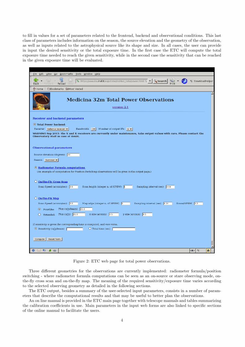
to fill in values for a set of parameters related to the frontend, backend and observational conditions. This lastclass of parameters includes information on the season, the source elevation and the geometry of the observation,as well as inputs related to the astrophysical source like its shape and size. In all cases, the user can providein input the desired sensitivity or the total exposure time. In the first case the ETC will compute the totalexposure time needed to reach the given sensitivity, while in the second case the sensitivity that can be reachedin the given exposure time will be evaluated.

Figure 2: ETC web page for total power observations.

Three different geometries for the observations are currently implemented: radiometer formula/positionswitching - where radiometer formula computations can be seen as an on-source or stare observing mode, on-the-fly cross scan and on-the-fly map. The meaning of the required sensitivity/exposure time varies accordingto the selected observing geometry as detailed in the following sections.

The ETC output, besides a summary of the user-selected input parameters, consists in a number of param-eters that describe the computational results and that may be useful to better plan the observations.

An on line manual is provided in the ETC main page together with telescope manuals and tables summarizingthe calibration coefficients in use. Main parameters in the input web forms are also linked to specific sectionsof the online manual to facilitate the users.

4

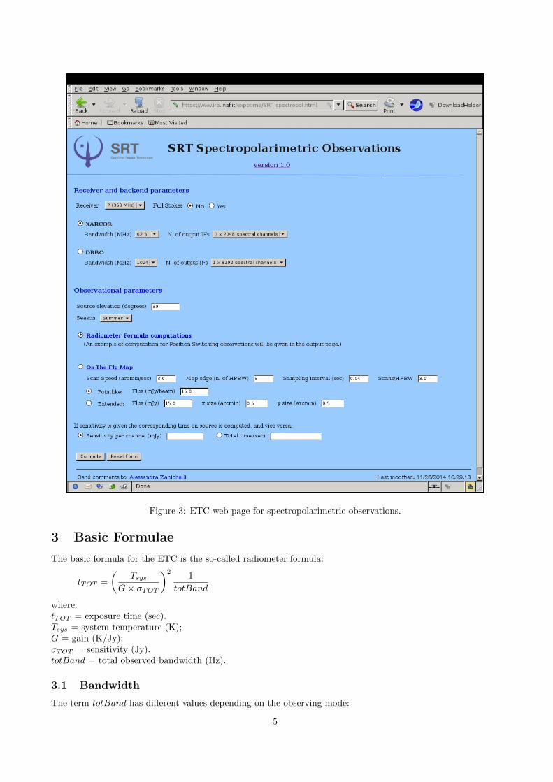
Figure 3: ETC web page for spectropolarimetric observations.

3 Basic Formulae

The basic formula for the ETC is the so-called radiometer formula:

tTOT =(

TsysG× σTOT

)2 1totBand

where:tTOT = exposure time (sec).Tsys = system temperature (K);G = gain (K/Jy);σTOT = sensitivity (Jy).totBand = total observed bandwidth (Hz).

3.1 Bandwidth

The term totBand has different values depending on the observing mode:

5

Continuum (no polarimetry): totBand = ∆ν ×NIFPolarimetry: totBand = 2×∆νSpectroscopy (no polarimetry): totBand = ∆νch ×NIFSpectropolarimetry: totBand = 2×∆νch

where:∆ν = observed bandwidth (Hz);∆νch = spectroscopic channel bandwidth (Hz);NIF = number of IF.In the following computations, totBand assumes the value corresponding to the user-selected observing mode.

3.2 System Temperature

Theoretically, the system temperature of a telescope changes with the telescope elevation according to theatmospheric emission, following:

Tsys = Trec + Tatm = Trec +[Tm

(1− e

−τsin(El)

)]where:Trec = receiver temperature (K);Tatm = atmospheric brightness, expressed as a temperature (K);Tm = average atmospheric temperature which takes into account also the effects of the higher trophosphericlayers (K);τ = atmospheric opacity;El = source elevation at the epoch of the observation.For receivers working below 22 GHz we assume that the seasonal variations of the atmospheric opacity arenegligible, and system temperature is given in the form of tabulated values as a function of source elevationonly. In this case, the user gives in input to the ETC the elevation at which the observation will be conducted(see next paragraphs) and the ETC selects among tabulated values the Tsys best matching the user-selectedelevation.When observing at 22 GHz, the seasonal variation of the atmospheric opacity is explicitly taken into accountin the Tsys computations. In such cases, the user selects both the source elevation and the season of theobservation. Average opacity values for the various seasons (Spring, Summer, Autumn, Winter) are available inthe ETC database and are selected on the basis of the ETC user-input parameters. For SRT, we use seasonaltabulated values also for Tm, while for Medicina we adopt a fixed Tm = 290 K throughout the year.

3.3 Receiver Gain

Receiver gain is computed differently for SRT and Medicina telescopes. For Medicina, the ETC uses thepolynomial formula:

G(El) = DPFU ×[(a× El)2 + (b× El) + c

]where El is the source elevation and DPFU , a, b, and c are tabulated coefficients for each receiver.In the case of SRT, gain is approximately constant at any elevation as it employs active mirrors, thus eachreceiver is characterized by a single gain value which is used by the ETC without the need to apply the aboveformula.

4 Radiometer Formula + Position Switching Computations

Computations in this case are done by simply applying the radiometer formula to the user-selected values. Inthis case, the input sensitivity/exposure time are intended to be on-source. In addition, an example of PositionSwitching observation is evaluated, assuming to perform an ON-OFF-OFF-ON cycle. Figure 4 illustrates thegeometry of a Position Switching observation.

6

Figure 4: Example of a Position Switching observation.

The ON position corresponds to the on-source one, while the OFF observation is executed at a nearby positionon the empty sky. The OFF position is assumed to be at a distance of 5 beamsizes from the ON one. An ON-OFF-OFF-ON sequence is assumed to minimize the time requested to move the telescope between consecutivepositions.

4.1 Input Parameters

The user provides in input:

1) the desired sensitivity σTOT (mJy) OR the desired time tTOT (sec).

4.2 Computations: given σTOT evaluate tTOT

The radiometer formula is used to compute the exposure time needed to reach a given sensitivity:

tTOT =(

TsysG× σTOT

)2 1totBand

4.3 Computations: given tTOT evaluate σTOT

By reverting the radiometer formula:

σTOT =(TsysG

) √1

totBand× tTOT

4.4 Position Switching computations

An example case for Position Switching observations is also computed as a particolar case for the radiometerformula mode.For Position Switching computations we assume a cycle of four exposures acquired in the sequence: ON-OFF-OFF-ON and combined as [(ON1-OFF1) + (ON2-OFF2)]/2 to get the final result. We also assume that thetime spent on each position is the same (tON = tOFF ), that measurements are independent and that they haveidentical uncertainties.The r.m.s. on the frame resultant from one (ON-OFF) subtraction is:

σON−OFF =√σ2ON + σ2

OFF = σON ×√

2

The r.m.s. on the frame resultant from the average of the two (ON-OFF) subtractions, i.e. the r.m.s. of oneON-OFF-OFF-ON cycle is, according to the error propagation for the mean:

σcycle =

√12× σ2

ON−OFF =

√12× 2× σ2

ON = σON

A) If the user-selected input sensitivity is intended to be reached in one complete ON-OFF-OFF-ON cycle ofPosition Switching, i.e. σcycle = σTOT , tcycle is computed as:

tcycle = 2× (tON + tOFF + tshift) + tprep

The value of tON = tOFF is computed by obtaining σON from the above equation for σcycle and applying the:

tON =(TsysG

)2 1σ2ON × totBand

7

The other terms in tcycle are: tprep, which is the instrument setup time, currently set to zero for Medicinaand SRT telescopes (as of ETC v1.0) and tshift, the slewing time needed to move from one position to thenext. The value for tshift is computed by means of the uniformly accelerated motion formula assuming thatthe OFF position is 5 beamsizes away from the ON position:

tshift =

√(5×HPBW )

2MaxAcc

The value of the maximum acceleration is set inside the ESCS/Nuraghe CommonDataBase (CDB). For Medicinaand SRT we consider as maximum values for the acceleration along the scan axis MaxAcc = 0.4 deg/sec2 andMaxAcc = 0.25 deg/sec2 respectively. These values have been set to be significantly lower than the actualmaximum accelerations allowed by the mount motors, in order to guarantee a smooth and precise execution ofthe acceleration ramp.

B) In the opposite case in which the user-selected input exposure time is intended to be used for the executionof a complete ON-OFF-OFF-ON cycle of Position Switching, tcycle = tTOT . The value for σON to be insertedin the σcycle equation is evaluated as:

σON =(TsysG

) √1

totBand× tON

where tON is obtained by reverting the equation for tcycle:

tON = [tcycle − (2× tshift)− tprep]/4

4.5 Output Parameters

When selecting the radiometer formula computations, the following parameters are given in output:

- Receiver gain (K/Jy), system temperature (K) and beam HPBW (arcmin) taken from tabulated valuesfor the selected receiver.

- Actual elevation (deg) used for computations: this parameter may slightly differ from the user-selectedone. Values for Tsys are tabulated at different values of the elevation, typically every 5 degrees. Amongthe tabulated values, the ETC looks for the Tsys which was measured at the elevation closest to theuser-selected one.

- Estimate of the Confusion Noise (mJy) at the selected frequency (not yet implemented for Medicina).

- Time on Source (sec) or Sensitivity (mJy) computed according with the selected input values.

- Example case for Position Switching Observations, in which an estimate of the total time needed tocomplete an ON-OFF-OFF-ON cycle is given. This estimate currently does not include the system setuptime.

5 On-The-Fly Cross Scan computations

Each scan is composed by two orthogonal subscans, to form a cross: the source is supposed to be located at theintersection of the cross. To reach a given sensitivity (or exposure time) many consecutive Cross Scans may berequired.An example of Cross Scan geometry is shown in Figure 5, where two consecutive crosses are executed over thesame position (the small displacement between the blue and red crosses is for visualization purposes) and eacharrow represents a subscan.


For OTF Cross Scan computations the user provides in input:

1) the length of each subscan: subscanLength (expressed in units of HPBW for the selected receiver);

8

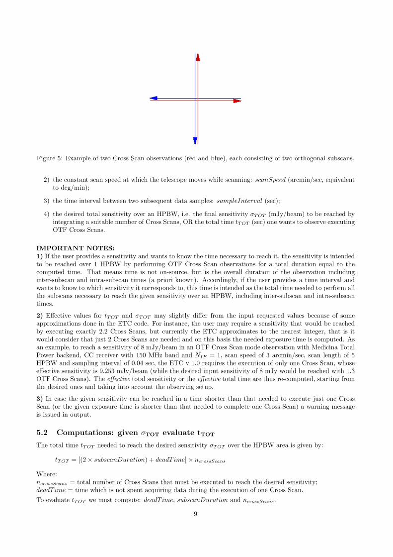
Figure 5: Example of two Cross Scan observations (red and blue), each consisting of two orthogonal subscans.

2) the constant scan speed at which the telescope moves while scanning: scanSpeed (arcmin/sec, equivalentto deg/min);

3) the time interval between two subsequent data samples: sampleInterval (sec);

4) the desired total sensitivity over an HPBW, i.e. the final sensitivity σTOT (mJy/beam) to be reached byintegrating a suitable number of Cross Scans, OR the total time tTOT (sec) one wants to observe executingOTF Cross Scans.

IMPORTANT NOTES:1) If the user provides a sensitivity and wants to know the time necessary to reach it, the sensitivity is intendedto be reached over 1 HPBW by performing OTF Cross Scan observations for a total duration equal to thecomputed time. That means time is not on-source, but is the overall duration of the observation includinginter-subscan and intra-subscan times (a priori known). Accordingly, if the user provides a time interval andwants to know to which sensitivity it corresponds to, this time is intended as the total time needed to perform allthe subscans necessary to reach the given sensitivity over an HPBW, including inter-subscan and intra-subscantimes.

2) Effective values for tTOT and σTOT may slightly differ from the input requested values because of someapproximations done in the ETC code. For instance, the user may require a sensitivity that would be reachedby executing exactly 2.2 Cross Scans, but currently the ETC approximates to the nearest integer, that is itwould consider that just 2 Cross Scans are needed and on this basis the needed exposure time is computed. Asan example, to reach a sensitivity of 8 mJy/beam in an OTF Cross Scan mode observation with Medicina TotalPower backend, CC receiver with 150 MHz band and NIF = 1, scan speed of 3 arcmin/sec, scan length of 5HPBW and sampling interval of 0.04 sec, the ETC v 1.0 requires the execution of only one Cross Scan, whoseeffective sensitivity is 9.253 mJy/beam (while the desired input sensitivity of 8 mJy would be reached with 1.3OTF Cross Scans). The effective total sensitivity or the effective total time are thus re-computed, starting fromthe desired ones and taking into account the observing setup.

3) In case the given sensitivity can be reached in a time shorter than that needed to execute just one CrossScan (or the given exposure time is shorter than that needed to complete one Cross Scan) a warning messageis issued in output.


The total time tTOT needed to reach the desired sensitivity σTOT over the HPBW area is given by:

tTOT = [(2× subscanDuration) + deadT ime]× ncrossScans

Where:ncrossScans = total number of Cross Scans that must be executed to reach the desired sensitivity;deadT ime = time which is not spent acquiring data during the execution of one Cross Scan.To evaluate tTOT we must compute: deadT ime, subscanDuration and ncrossScans.

9

- Evaluate deadTime:The parameter deadT ime is the time which is not spent acquiring data during the execution of one Cross Scan.It is given by the sum of two terms: interSubscanT ime and intraSubscanT ime. The first term is given by theduration of the acceleration/deceleration ramps taking place before/after the actual subscans, and is determinedas a function of the scanning speed and of a given fraction of the maximum acceleration allowed by the mount,specific for each telescope.For Medicina and SRT we consider the maximum acceleration MaxAcc to be 0.4 deg/sec2 and 0.25 deg/sec2

respectively, and we use one tenth of the maximum acceleration to compute the ramps (as the systemitself does, to guarantee the maximum precision):

rampTime =speed

0.1×MaxAcc=speed

0.025

The execution of each subscan implies to perform 2 ramps, so:

interSubscanT ime =2× speed

0.025

The term intraSubscanT ime is an indicative intra-scan slewing time (i.e. performed at full MaxAcc), whichtakes into account the change in position among subscans. By reverting the formula for the uniformly acceleratedmotion (s = 1

2 a t2) and considering that s (the intra-scan path) in this case is the hypotenuse of a triangle

whose sides are the two half-subscans:

intraSubscanT ime =

√√2× subScanLength

MaxAcc=

√√2× subscanLength

0.25

It is now possible to estimate the overall dead time for 1 Cross Scan: it is given by twice the interSubscanT ime(two sub-scans form one Cross Scan) plus once the intraSubscanT ime (the telescope changes position betweensubscans once per Cross Scan).

deadT ime = (2× interSubscanT ime) + intraSubscanT ime

- Evaluate subscanDuration:The duration of a single subscan is easily computed as:

subscanDuration = subscanLength / scanSpeed

where we recall that subscanLength is given in units of HPBW (see Sect. 5.1).

- Evaluate ncrossScans:First compute ttotHPBW = time spent on 1 HPBW to reach the desired sensitivity σTOT :

ttotHPBW =

(σ2HPBW,singleSubscan

σ2TOT

)tHPBW

Where the time spent on HPBW during each subscan is:

tHPBW = HPBW/scanSpeed

The sensitivity over an HPBW for each subscan is given by:

σHPBW,singleSubscan = σi

√sampleInterval

tHPBW

And σi, given by the radiometer formula, is the sensitivity per sampling interval:

σi =(TsysG

) √1

totBand× sampleInterval

Where totBand takes the value proper to the observing mode, as defined in Section 3.

10

Having computed the time that is necessary to spend over one HPBW area to reach the σTOT sensitivity, thenumber of necessary subscans is computed dividing it by the time spent on one HPBW during each subscan.

nsubscans =ttotHPBWtHPBW

The number of complete Cross Scans (i.e. the number of couples of orthogonal subscans)is:

ncrossScans = (nsubscans + 1)/2

Results are rounded up in order to always obtain an integer number of complete Cross Scans.


The parameter tTOT is the overall observing time and thus includes also deadT ime. The actual sensitivityσTOT must be computed using the effective time spent on Cross Scans, i.e. excluding intraSubscanT ime andinterSubscanT ime. First we need to compute how many Cross Scans can be executed in the given tTOT :

nCrossesInExptime =tTOT

singleCrossTotalT ime

where singleCrossTotalT ime is the total time to execute one Cross Scan (including its overheads):

singleCrossTotalT ime = (2× subscanDuration) + deadT ime

and deadT ime is computed as in Sect. 5.2. The value of nCrossesInExptime is rounded to the nearest integer.The sensitivity σTOT is thus:

σTOT =σHPBW,singleSubscan√nCrossesInExptime


When selecting the On-The-Fly Cross Scan computations, the following parameters are given in output:

- Receiver gain (K/Jy), system temperature (K) and beam HPBW (arcmin) from tabulated values for theselected receiver.



- Total Time (sec) and Sensitivity (mJy/beam) for 1 Cross Scan. These are the time needed to complete 1Cross Scan and the sensitivity that can be reached over 1 Cross Scan. They are computed, according to thequantities derived above, as singleCrossTotalT ime and singleCrossRms = σHPBW,singleSubscan /

√2.

- Total number of Cross Scans: the number of Cross Scans nCrossesInExptime (each one being made of acouple of orthogonal subScans) to be executed and combined in order to reach the desired input sensitivity/ exposure time. A minimum of 1 Cross Scan is imposed.

- Total dead Time (sec) is the dead time spent for the execution of the required number of Cross Scans, i.e.deadT ime×nCrossesInExptime. It takes into account the slewing time plus the acceleration/decelerationramps.

- Total OTF Cross Scan Time (sec) is the total observing time that is needed to reach the user-selected sensi-tivity over nCrossesInExptime Cross Scans. Conversely, Total OTF Cross Scan sensitivity (mJy/beam)is the sensitivity obtained over nCrossesInExptime Cross Scans given the user-selected observing time.

11

- Effective Total OTF Cross Scan Time (sec) or Effective Total OTF Cross Scan sensitivity (mJy/beam).These numbers are computed to account for some approximations made by the code that may affect theplanning of the observations. For instance, currently the number of Cross Scans is rounded to the nearestinteger (not rounded upwards to the nearest integer), thus the effective total sensitivity or the effectivetotal time are re-computed, starting from the desired ones and taking into account the observing setup.Effective values may slightly differ from the input requested values because of the above approximations,see also notes in Sect. 5.1.

6 On-The-Fly Map computations

Each map is composed by a sequence of back-and-forth On-The-Fly subscans. Each subscan is shifted withrespect to the previous one in order to fully cover the desired sky region.An example of On-The-Fly Map geometry is shown in Figure 6, where each arrow represents a subscan.

Figure 6: Example of an On-the-Fly Map observation.


For OTF Map computations the user provides in input:

1) the scan speed at which the telescope moves during the Cross Scan: scanSpeed (arcmin/sec, equivalentto deg/min);

2) the time interval between two subsequent samples: sampleInterval (sec);

3) the map edge, i.e. the map span on each side of the source, expressed in number of HPBW: mapEdge.The source size and mapEdge are used to compute the size of the map (see computations below).

4) the number of scans for each HPBW, corresponding to the HPBW sampling: linesPerHPBW .

5) source parameters:

- source geometry: extended or pointlike;

- source flux: Flux, in mJy/beam for pointlike sources or in mJy for extended sources (intended asthe source integrated flux). Flux values are only used to compute the total S/N;

- source sizes: for extended sources sizex, sizey (arcmin). The size of pointlike sources is set by defaultto the HPBW value for the selected receiver. The source size and mapEdge are used to compute thesize of the map.

6) the desired total sensitivity over one HPBW, i.e. the sensitivity to be reached over an HPBW area, σTOT(mJy/beam). In this case the ETC computes how many OTF maps are needed to reach that sensitivity.Alternatively, one can provide the total time to be spent in OTF map mode with the selected observingsetup, tTOT (sec). In this case the ETC computes how many maps will be completed in that time intervaland what value of the final sensitivity is going to be reached.

12

IMPORTANT NOTES:1) Currently, square maps only are allowed. As detailed in Sect. 6.2, the maximum source size (i.e. one HPBWfor pointlike sources or the maximum between sizex and sizey for extended sources) and mapEdge are used tocompute the size of the map.

2) if the user provides a sensitivity and wants to know the time necessary to reach it, the sensitivity is intendedto be reached over an HPBW by performing OTF Map observations for a duration equal to the computed time.That means time is not on-source, but is the overall duration of the observation including ”dead time” (a prioriknown). Accordingly, if the user provides a time and wants to know to which sensitivity it corresponds, time isintended as the total time needed to perform all the map observations necessary to reach the given sensitivityover an HPBW, including ”dead time”.

3) Effective values for tTOT and σTOT may slightly differ from the input requested values because of someapproximations done in the ETC code. For instance, the user may require a sensitivity that would be reachedby executing exactly 2.2 OTF maps, but currently the ETC approximates to the nearest integer, that is it wouldconsider that just 2 maps are needed and on this basis the needed exposure time is computed. Similarly, theETC requires that at least one map is executed even if the desired sensitivity could be reached in a shorter time.As an example, to reach a sensitivity of 7 mJy/beam in an OTF Map mode observation of a pointlike sourcewith Medicina Total Power backend, CC receiver with 150 MHz band and NIF = 1, scan speed=3 arcmin/sec,map edge=5 HPBW, sampling interval of 0.04 sec, 3 scans per HPBW, the ETC v 1.0 requires the execution ofonly one OTF map, whose effective sensitivity is 7.555 mJy/beam (while the desired input sensitivity would bereached with 1.15 OTF maps). The effective total sensitivity or the effective total time are thus re-computed,starting from the desired ones and taking into account the observing setup.


The time tTOT can be expressed as:

tTOT = nmap × t1

where:nmap = number of maps to be combined to reach σTOT .t1 = time needed to complete one map given the observing parameters, including dead time.To evaluate tTOT we must compute: nmap and t1.

- Evaluate nmap: The expression for σTOT can be written as:

σTOT =σ1√nmap

where σ1 is the sensitivity reached over one HPBW in a single map assuming that each beam size is sampledwith linesPerHPBW points (i.e. linesPerHPBW scans are needed to sample one HPBW). It can be easilycomputed by means of the sensitivity per HPBW reached in a single subscan:

σ1 =σHPBW,singlesubscan√linesPerHPBW

where the formula for σHPBW,singlesubscan is the same as in the OTF Cross Scan case. By substituting σ1 andσTOT in the above formula, the number of maps nmap can be evaluated.

- Evaluate t1: The time needed to complete 1 map, including dead time, is:

t1 = (tsingleScan + deadT ime)× linesPerMap

where:

tsingleScan = mapSize / scanSpeed

linesPerMap =mapSize

HPBW× linesPerHPBW

deadT ime = interSubscanT ime+ intraSubscanT ime

13

where now, differently to what happened in the OTF Cross Scan case for the computation of deadT ime, thepath to be performed in uniformly accelerated motion is exactly given by the transverse distance between twosubscans (no more need to build a triangle). The parameter intraSubscanTime is thus:

intraSubscanT ime =

√HPBW

linesPerHPBW× 2MaxAcc

Note that the formula for t1 makes an approximation which has a negligible effect on computations. The correctone would be t1 = (tsingleScan + interSubscanT ime) linesPerMap + intraSubscanT ime (linesPerMap − 1)since the last subscan does not require additional turning time once completed.Map size for pointlike sources is:

mapSize = HPBW + 2× (mapEdge×HPBW )

While for extended sources:

mapSize = [max(sizex, sizey)] + 2× (mapEdge×HPBW )

If the user select the extended source option but both the given source sizes happen to be smaller than thebeamsize of the chosen receiver, the source is considered unresolved and mapSize is computed as for pointlikesources.Finally, the Signal to Noise ratio over 1 HPBW area on the combined nmap is computed as:

pointlike sources :S

N=Flux

σTOT

extended sources :S

N=(Flux×HPBWarea

sourceArea

)× 1σTOT

where:

sourceArea = π × (0.5× sizex)× (0.5× sizey)

HPBWarea = π × (0.5×HPBW )2

NOTE that the formula for extended sources gives an approximated result when sizex or sizey is sensiblysmaller than HPBW or the source is elongated and it actually does not fill ”well” the beam. Results areaccurate if the extended source completely fills the beam in both directions.


The parameter tTOT is the overall observing time and thus includes also deadT ime. The actual sensitivityσTOT must be computed using the effective time spent on the map, i.e. excluding intraSubscanT ime andinterSubscanT ime. First we need to compute how many maps can be executed in the given tTOT , rounded tonearest integer (and at least equal to 1):

nmap = nearest integer(tTOT / t1)

where t1 is the time needed to complete one map given the observing parameters, including dead time, and iscomputed as in Sect. 6.2.The sensitivity σTOT is thus computed as:

σTOT =σ1√nmap

where σ1 is the sensitivity reached over one HPBW in a single map, computed as in Sect. 6.2.

14


When selecting the On-The-Fly Map computations, the following parameters are given in output:

- Receiver gain (K/Jy), system temperature (K) and beam HPBW (arcmin) from tabulated values for theselected receiver.



- Map size (arcmin): maps are defined as squares centered on the source. Depending on the source geometry,the map size mapSize is computed according to the above formulae.

- Number of subscans per map: depending on map and beam sizes and on the desired number of scans perHPBW the parameter linesPerMap is computed.

- Total Time (sec) and Sensitivity (mJy/beam) for 1 Map. These are the quantities t1 and σ1 and refer tothe time needed to complete one single map and to the sensitivity than can be reached on a single map.

- Total number of Maps: the number of maps nmap (each one being made of linesPerMap subscans) to beexecuted and combined in order to reach the desired input sensitivity / exposure time. A minimum of 1map is imposed.

- Total dead Time (sec) is the dead time spent for the execution of the required number of Maps, i.e.deadT ime× nmap. It takes into account the slewing time plus the acceleration/deceleration ramps. Theparameter deadT ime is computed in a slightly different way than for the OTF Cross Scan case, seecomputations above.

- Total OTF Map Time (sec) is the total observing time needed to reach the user-selected sensitivity overnmap OTF maps. Conversely, Total OTF Map sensitivity (mJy/beam) is the sensitivity obtained overnmap OTF maps given the user-selected observing time.

- Effective Total OTF Map Time (sec) or Effective Total OTF Map sensitivity (mJy/beam). These numbersare computed to account for some approximations made by the code that may affect the planning of theobservations. For instance, currently the number of maps is rounded to the nearest integer (not roundedupwards to the nearest integer), thus the effective total sensitivity or the effective total time are re-computed, starting from the desired ones and taking into account the observing setup. Effective valuesmay slightly differ from the input requested values because of the above approximations, see also notes inSect. 6.1.

- Source Signal-to-Noise Ratio over 1 HPBW area on the combined final map. This is the signal-to-noiseratio S

N over nmap combined maps and inside a circular area of HPBW diameter. Depending on sourcegeometry, it is computed in terms of source flux density and total sensitivity.

7 Confusion Noise computations

Confusion noise computations are currently implemented for SRT, and will be extended to the Medicina telescopein ETC version 1.1 to be released in summer 2015.The rms width of the point-source confusion amplitude distribution calculated by Condon (1974) at the genericfrequency ν is:

σc,ν =(q3−γ

3− γ

) 1γ−1

(kΩbγ − 1

) 1γ−1

(ν

ν0

)−αwhere q is the signal-to-noise ratio under which we expect confusion, Ωb the beam solid angle, α the spectralindex (with S = S0ν

−α), and k and γ are the parameters of the power-law differential source counts calculatedat the frequency ν0:

nν0(S) = kS−γ

15

Note that for the ETC computations we assumed q = 5.To calculate the rms confusion at various frequencies the following power-law differential counts have been used:

- at 1.4 GHz we used the distribution given by Bondi et al. (2003) for S > 0.6 mJy:

n1.4 GHz = (75.86± 1.08)(

S

mJy

)−(1.79±0.05)

mJy−1deg−2

- at 5 GHz we extrapolated the confusion limit from the distribution at 1.4 GHz given by Bondi et al.(2003) for S < 0.6 mJy

n1.4 GHz = (57.54± 1.07)(

S

mJy

)−(2.28±0.04)

mJy−1deg−2

- at 20 GHz, we extrapolated the confusion limit from the distribution at 15 GHz given by Davies et al.(2011) for 0.5mJy < S < 2.8mJy:

n15 GHz = 376(S

Jy

)−1.80

Jy−1sr−1

- at 327 MHz, we extrapolated the confusion limit from the distribution at 333 MHz obtained by fitting thedifferential normalized source counts versus the flux given by Owen et al. (2009):

n333MHz = 1546(S

Jy

)−1.88

Jy−1sr−1

References

Bondi, M., Ciliegi, P., Zamorani, G., et al. 2003, A&A, 403, 857.

Condon, J. J. 1974, ApJ, 188, 279.

Davies, M. L., Franzen, T. M. O., et al. 2011, MNRAS, 415, 2708.

Owen, F. N., Morrison, G. E., Klimek, M. D., & Greisen, E. W. 2009, AJ, 137, 4846.

16

Documents

SINGLE DISH EXPOSURE TIME CALCULATOR User Manual · SINGLE DISH EXPOSURE TIME CALCULATOR User Manual Release 1.0 A. Zanichelli 1, S. Righini , K.-H. Mack 1, A. Orfei , V. Vacca2 in