Singapore Lecture2

Applied Financial Econometrics using Stata2. Working with Data

Stan Hurn

Queensland University of Technology& National Centre for Econometric Research

Hurn (NCER) Applied Financial Econometrics using Stata 1 / 43

1 Data Sources

2 General Data Issues

3 Time Series Data

4 Reconfiguring Data


Data Sources

Basic Principle

Stata stores data in .dta files.One of the implications of the concern for reproducible work: avoidaltering data in a spreadsheet. Rather, you should transfer external datainto the Stata environment as early as possible in the process of analysis,and only make changes to the data with do-files that can give you an audittrail of every change made.


Data Sources

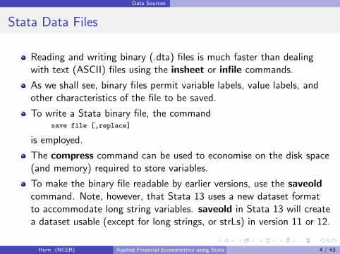
Stata Data Files

Reading and writing binary (.dta) files is much faster than dealingwith text (ASCII) files using the insheet or infile commands.

As we shall see, binary files permit variable labels, value labels, andother characteristics of the file to be saved.

To write a Stata binary file, the commandsave file [,replace]

is employed.

The compress command can be used to economise on the disk space(and memory) required to store variables.

To make the binary file readable by earlier versions, use the saveoldcommand. Note, however, that Stata 13 uses a new dataset formatto accommodate long string variables. saveold in Stata 13 will createa dataset usable (except for long strings, or strLs) in version 11 or 12.


Data Sources

Loading Data

For data saved in other file formats (such as SAS or SPSS etc.) Statasupports a handy bit of software called Stat Transfer.

http://www.stata.com/products/stat-transfer/

Unfortunately Stat Transfer doesn’t come with Stata 13 and is anadditional expense. Neither does it handle EViews files at this point!From a data perspective, two really useful commands are:

1 webuse

2 freduse


http://www.stata.com/products/stat-transfer/

Data Sources

webuse

Specify URL from which dataset will be obtainedwebuse set [http://]url[/]

then simply issue the command and the name of the filewebuse ‘‘mydata.dta’’

Stata will automatically use the specified URL to access the web andload the named data file (which must be a .dta file).

All the data used in this set of lectures may be accessed using theURL

http://www.ncer.edu.au/stata-resources/data/Singapore


http://www.ncer.edu.au/stata-resources/data/Singapore

Data Sources

freduse

An important source of macro and financial data is the St. Louis FederalReserve database (FRED)

http://research.stlouisfed.org/fred2

To use a facility that allows you to download data directly from thedatabase you need to download and install a package from the web

findit freduseclick on st0110 from http://www.stata-journal.com/software/sj6-3

This will install the package.There is also a YouTube video on how to use this facility

YouTubeVideo


http://research.stlouisfed.org/fred2

http://www.youtube.com/watch?v=iiizhsX-I00

Data Sources

Example -webuse

The following series of commands in a .do file// real us gdp

clearwebuse set http://www.ncer.edu.au/stata-resources/data/Singaporewebuse "usrealgdp.dta", replace

will go to the NCER website and load the Stata usrealgdp.dta file.


Data Sources


Data Sources

Example -freduse

The Federal Reserve Economic Data can be accessed to find a tag for realUS gpd. FRED

// real us gdp

freduse GDPC1

One thing to be a little careful about is the date convention used by FRED.


http://research.stlouisfed.org/fred2/series/GDPC1

Data Sources


General Data Issues

Missing Data

Missing value codes in Stata appear as the dot (.)

the missing function mi(varname) will return 1 if the observation is amissing value, 0 otherwise

the missing value in fact takes the value positive infinity, so in thepresence of missing data you do not want to say

generate hiprice = (price > 10000)

but rathergenerate hiprice = (price > 10000) if price <.

or preferablygenerate hiprice = (price > 10000) if !mi(price)

which then generates an indicator (dummy) variable equal to zero forlow-prices and missing when price is missing.


General Data Issues

More on Missing Data

Stata actually allows for allows for multiple missing value codes (.a,.b, .c, ..., .z) The standard missing value code (.) is the smallest ofthese. This is useful if you wish to encode in the data the fact thatdata are missing for different reasons.

Spreadsheet files often use NA to denote missing values, while insome datasets codes such as -9, -999, or -0.001 are used.

the former is problematic because Stata will read an entire variable as astring and not a numeric value if NA appears anywhere .... (this isparticularly irksome when dealing with Excel spreadsheets).the latter instances are particularly worrisome as they may not bedetected unless the variables? values are carefully scrutinized.

Stata provides two further commands to deal with missing values,namely, the mvdecode and mvencode commands. They allow youto map various missing values into numeric values and vice versa.


General Data Issues

Labels

Variable labelsis a character string (maximum 80 characters) which describes thevariable

label variable varname "text"

Variable labels are used to identify the variable in printed output andgraphs

Value labelsassociate numeric values with character strings

label define sexlbl 0 male 1 femalelabel values sex sexlbl

they exist separately from variables, so that the same mapping ofnumerics can be applied to a set of variables (e.g. 1=verysatisfied...5=not satisfied may be applied to all responses to questionsabout consumer satisfaction).


General Data Issues

Notes on Individual Series

The command

notes : text

will enter notes on the dataset.

. notes list _dta

_dta:1. This file was constructed from an excel data file provided by Mardi Dungey. It allows reproduction of the

results of estimating a SVAR of the Australian economy developed in a series of papers by Mardi Dungey andAdrian Pagan (2000, 2009) published in the Economic Record.

2. Dungey, M. and Pagan, A.R. (2000) A Structural VAR of the Australian Economy, Economic Record, 76, 321-342.3. Dungey, M. and Pagan, A.R. (2009) Revisting an SVAR of the Australian Economy, Economic Record, 85, 1-20.


General Data Issues

Notes on Individual Series

The command

notes variablename: text

will enter notes on the named variable.

. notes rgdp tot uscpi djindus

rgdp:1. Real US GDP in US$ 1979Q3 to 2006Q4 (seasonally adjusted). Source - DATASTREAM

tot:1. Australian Terms of Trade 1979Q3 to 2006Q4 (seasonally adjusted). Source - RBA Bulletin

uscpi:1. US Consumer Price Index 1979Q3 to 2006Q4 (not seasonally adjusted). Source - DATASTREAM

djindus:1. Dow Jones Industrial Price Index 1979Q3 to 2006Q4. Source - DATASTREAM


General Data Issues

Order

Stata has one important feature that will be foreign to people used tocoding in Gauss or Matlab. The order of variables in the datasetmatters.

This is because you can use hyphenated lists to include all variablesbetween first and last.

You can also use wildcards to refer to all variables with a certainprefix. If you have variables pop60, pop70, pop80, pop90, you canrefer to them in a varlist as pop* or pop?0.

The order and move commands can alter the order of variables.


Time Series Data

Dates

Stata supports date (and time) variables and the creation of a timeseries calendar variable.

Dates are expressed, as they are in Excel, as the number of days froma base date. In Stata’s case, that date is 1 Jan 1960 (likeUnix/Linux). Negative numbers represent dates and times beforeJanuary 1, 1960, and positive numbers represent dates and timesafterward.

You may set up data on an annual, half-yearly, quarterly, monthly,weekly or daily calendar, as well as a calendar that merely uses theobservation number. High-frequency data are also supported.

An observation-number calendar is generally necessary forbusiness-daily data where you want to avoid gaps for weekends,holidays etc. which will cause lagged values and differences to containmissing values (creating two calendar variables for the same timeseries data can be useful).


Time Series Data

Dates and Times


Time Series Data

tsset

Useful commands to create date variables are

gen daten = %tq(1970q1) + _n-1 (quarterly)

gen daten = %tm(1970m1) + _n-1 (monthly)

gen daten = %tw(1970w1) + _n-1 (weekly)

gen daten = _n (observation number)

After creating the date variable you need to tell Stata that the data youhave is time series data. You do this using the command

tsset daten, monthly


Time Series Data

Reading Dates

Say you have date strings like ”November 3, 2010”, ”11/3/2010” or”2010-11-03 08:35:12” in a file and you wish to read these into Statadate format.

This can be achieved using the date function. The date functiontakes two arguments, the string to be converted, and a series ofletters called a ”mask” that tells Stata how the string is structured.In a date mask, Y means year, M means month, D means day and #means an element should be skipped.

gen date1=date(dateString1,"MDY")gen date2=date(dateString2,"MDY")gen date3=date(dateString3,"YMD###")

Be aware that if you have a string which works with two-digit dates,Stata can become confused .... You can overcome this by adding anoptional third argument which specifies the largest year in the data.This way Stata will ensure that the last year is numbered correctly.


Time Series Data

Seasonal Dummies

The process of creating a set of quarterly or monthly dummy variables is abit more elaborate in Stata than in a package such as EViews.Assume there is a suitably defined and formatted date identifier calleddateid.

quarterly dummy variablesfor values i = 1/3 {gen seas‘i’ = (quarter(dofq(dateid)) == ‘i’)}

monthly dummy variablesfor values i = 1/11 {gen seas‘i’ = (month(dofm(dateid)) == ‘i’)}


Time Series Data

Business Days

A problem with Stata Version 12 and below was its inability to handlebusiness day calendars. This required a bit of trickery to overcome

running a calendar with both observations and date identifiersusing say FRED to create the date identifier

In Version 13 there is a new command bcal.

For example, bcal create creates a business calendar file from thecurrent dataset and describes the new calendar. If sp500.dta is adataset installed with Stata that has daily records on the S&P 500stock market index in 2001 business calendar for stock trading in2001 can be automatically created from this dataset as follows:

bcal create sp500, from(date) purpose(S&P 500 for 2001) generate(bizdate)


Time Series Data

Time Series Operators

The D., L., and F. operators may be used under a time seriescalendar (including panel data) to specify first differences, lags, andleads, respectively.

These operators understand missing data, and number lists: e.g.L(1/4).x is the first through fourth lags of x.

The time series operators respect the time series calendar, and willnot mistakenly compute a lag or difference from a prior period if it ismissing (this may be particularly important when working with paneldata).

You can refer to time-series operators on the fly, for example

regress y L(1/4).y

regress y L(-4/4).x

regress D.y L.y


Time Series Data

Basic Plotting

// load data

webuse set http://www.ncer.edu.au/stata-resources/data/Singapore

webuse usrealgdp.dta, clear

// declare data to be time series

tsset daten, quarterly

// plot real us gdp

twoway (line rgdp daten), name(realusgdp) ///

xtitle(" ") ytitle("$ Billions") title("Real U.S. GDP")

// graph export "realusgdp.pdf", as(pdf) replace

Could also use the

twoway tsline rgdp


Time Series Data

A few simple manipulations

// compute growth rate in gdp

gen gr = 400*(log(rgdp)-log(L1.rgdp))

label var gr "Growth rate of real US GDP"

twoway (line gr daten), name(growth) ///

xtitle(" ") ytitle("%") title("Growth Rate of Real U.S. GDP")

// graph export "growth.pdf", as(pdf) replace

// smooth growth rate with 7 period moving average

tssmooth ma c = gr, window(3 1 3)

label var c "US Business Cycle"

twoway (line c daten, lwidth(medthick)) ///

|| (line gr daten, lwidth(vthin)lpattern(dash)), name(cycle) ///

xtitle(" ") ytitle("%") title("U.S. Business Cycle")legend(off)


Time Series Data

Some annotation

// provide some annotation

gen max = 10

// major recessions

twoway (area max daten if tin(1973q3,1975q1), base(-5) color(gs12)) ///

(area max daten if tin(2007q3,2009q2), base(-5) color(gs12)) ///

(line c daten), xtitle(" ") ytitle("%") legend(off) ///

title("Major U.S. Contractions") name(g1,replace) nodraw

// major expansions

twoway (area max daten if tin(1991q2,2007q1), base(-5) color(eltgreen)) ///

(line c daten), xtitle(" ") ytitle("%") legend(off) ///

title("Major U.S. Expansion") name(g2,replace) nodraw

graph combine g1 g2, xcom ycom rows(2) cols(1)

graph export "realusgpdannotated.pdf", as(pdf) replace


Time Series Data

Snapshot of the log file


Time Series Data

Annotated gdp graph-5

05

10%

1950q1 1960q1 1970q1 1980q1 1990q1 2000q1 2010q1

Major U.S. Contractions

-50

510

%

1950q1 1960q1 1970q1 1980q1 1990q1 2000q1 2010q1

Major U.S. Expansion


Time Series Data

Graph Schemes


Reconfiguring Data

Manipulating Datasets

Stata only permits a single data set to be accessed at one time. How,then, do you work with multiple data sets?

At least one of the datasets to be combined must already have beensaved in Stata format.

Several commands are available, including append, merge, and joinby.


Reconfiguring Data

append

The append combines two Stata-format data sets that possess variables incommon, adding observations to the existing variables.

The datasets to be combined should share the same variable namesand datatypes (string vs. numeric). Appending these two datasetswith common variable names creates a single dataset containing all ofthe observations. It is important to note that “PRICE” and “price”are different variables, and one will not be appended to the other.

The same variables need not be present in both files, as long as asubset of the variables are common to the “master” and “using” datasets. Where required, the values of any variables which are notcommon are set to missing.


Reconfiguring Data

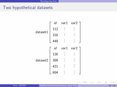
Two hypothetical datasets

dataset1

id var1 var2

112...

...

216...

...

449...

...

dataset2

id var1 var2

126...

...

309...

...

421...

...

604...

...


Reconfiguring Data

using append

We may append these datasets:

dataset

id var1 var2

112...

...

216...

...

449...

...

126...

...

309...

...

421...

...

604...

...

The rule for append, then, is that if datasets are to be combined, theyshould share the same variable names and datatypes (string vs. numeric).


Reconfiguring Data

merge

merge is Stata’s basic tool for working with more than one dataset.

merge works on a “master” dataset (the current contents ofmemory) and a single “using” dataset. This distinction is important.Stata’s default behaviour is to hold the master data inviolate anddiscard the using dataset’s copy of that variable. This may bemodified by the update option, which specifies that non-missingvalues in the using dataset should replace missing values in themaster, and the even stronger update replace, which specifies thatnon-missing values in the using dataset should take precedence.

the variable merge takes on integer values indicating whether anobservation appears in the master only, the using only, or appears inboth. This may be used to determine whether the merge has beensuccessful, or to remove those observations which remain unmatched.The merge variable must be dropped before another merge isperformed on this data set.


Reconfiguring Data

Two hypothetical datasets

dataset1

id var1 var2

112...

...

216...

...

449...

...

dataset2

id var3 var4 var5

112...

......

216...

......

449...

......


Reconfiguring Data

using merge

We may merge these datasets on the common merge key: in this case, theid variable:

merged dataset

id var1 var2 var3 var4 var5

112...

......

......

216...

......

......

449...

......

......

The rule for merge, then, is that if datasets are to be combined on one ormore merge keys, they each must have one or more variables with acommon name and datatype (string vs. numeric).


Reconfiguring Data

post file and post

A very useful capability is provided by the postfile and postcommands, which permit a Stata data set to be created in the courseof a program.

If you are simulating the distribution of a statistic, fitting a modelover separate samples, or bootstrapping standard errors, you may postcertain numeric values to a postfile within the looping structure usingthe command post.

This will create a separate Stata binary data set, which may then beopened in a later Stata run and analysed. Note, however, that onlynumeric expressions may be written to the postfile.


Reconfiguring Data

Panel Data

Data are often provided in a different orientation than that required forstatistical analysis. The most common example of this occurs with panel,or longitudinal, data, in which each observation conceptually has bothcross-section (i) and time-series (t) subscripts.

Different models applied to longitudinal data require differentorientations of those data.

SUR needs “wide” dataFixed–effects or random–effects regression models prefer that the databe stacked in the“long” format.

The reshape command allows you to transfer the data from “wide”to “long” format or vice versa.


Reconfiguring Data

Wide format

Consider this data fragment of U.S. state, with the unit?s name for therows and the year for the columns.This data is in wide form with the samemeasurement (population) for different years denoted as separate Statavariables.


Reconfiguring Data

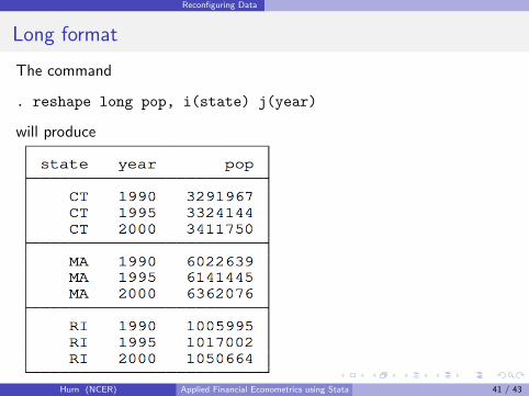
Long format

The command

. reshape long pop, i(state) j(year)

will produce


Reconfiguring Data

collapse

But what if you want to use average values for each time period,averaged over states?

The resulting dataset of T observations can be easily created by thecollapse command, which permits you to generate a new data setcomprised of summary statistics of speci?ed variables.

More than one summary statistic can be generated per input variableas collapse can produce counts means, medians, percentiles, extrema,and standard deviations.

collapse kills your dataset so be sure to save it before you use thecommand!


Reconfiguring Data

A word or two of caution

With the proper use of reshape, writing data out and reading themback in is not necessary in Stata. In situations beyond the simpleapplication of reshape, it may require some experimentation toconstruct the appropriate command syntax. This is all the morereason for enshrining that code in a do-file as some day you are likelyto come upon a similar application for reshape.

Stata provides two commands preserve and restore.

preserve preserves the data, guaranteeing that data will be restoredafter program terminationrestore forces a restore of the data when required.

These can be helpful in complex .do files.

Current advice from a contact in Stata suggests sparing use of thesecommands and saving the data instead!


Documents

Singapore Lecture2