Embed Size (px)
Citation preview

SinCHet: a MATLAB toolbox for single cell heterogeneity analysis
Background: Single-cell technologies allow characterization of transcriptomes and epigenomes for individual cells under different conditions and provide unprecedented resolution for researchers to investigate cellular heterogeneity in cancer. The SinCHet (Single Cell Heterogeneity) toolbox is developed in MATLAB and has a graphical user interface (GUI) for visualization and user interaction. It analyzes both continuous (e.g. mRNA expression) and binary omics data (e.g., discretized methylation data). The toolbox does not only quantify cellular heterogeneity using Shannon Profile (SP) at different clonal resolutions but also quantify heterogeneity differences using a D statistic between two populations. It is defined as the differences of areas under two SPs. This flexible tool provides a default clonal resolution using the change point of Profile of Shannon Difference (PSD) detected by multivariate adaptive regression splines model; it also allows user-defined clonal resolutions for further investigation. This tool provides insights into emerging or disappearing clones between conditions, and enables the prioritization of biomarkers for follow-up experiments based on heterogeneity or marker differences between and/or within cell populations.
Jiannong Li, Inna Smalley, Michael J. Schell, Keiran S. Smalley, Y. Ann Chen*. SinCHet: a MATLAB toolbox for single cell heterogeneity analysis.
Corresponding author: [email protected]
What's included on the webpage:
1. The pre-compiled standalone version SinCHet for users without MATLAB license.
2. The source code of our implementation of SinCHet for users with MATLAB license.
3. The example datasets consists of a published single-cell miRNA expression continuous data (gene_expression.xlsx) and discretized methylation data. Both datasets have 60 cells. Forty-one of them are EGFR mutant while the other 19 are wild type collected from the primary human lung adenocarcinomas. (Cheow, Courtois et al. 2016).
• Cheow, L. F., E. T. Courtois, Y. Tan, R. Viswanathan, Q. Xing, R. Z. Tan, D. S. Tan, P. Robson, Y. H. Loh, S. R. Quake and W. F. Burkholder (2016). "Single- cell multimodal profiling reveals cellular epigenetic heterogeneity." Nat Methods 13(10): 833-836.
License conditions:
The SinCHet software is freely available for non-profit academic use. For licensing opportunities, please contact [email protected] or [email protected] at Moffitt’s Innovation office
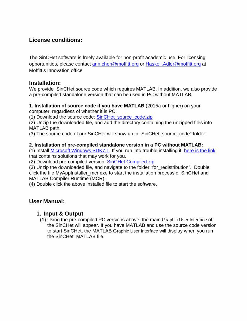
Installation: We provide SinCHet source code which requires MATLAB. In addition, we also provide a pre-compiled standalone version that can be used in PC without MATLAB. 1. Installation of source code if you have MATLAB (2015a or higher) on your computer, regardless of whether it is PC: (1) Download the source code: SinCHet_source_code.zip (2) Unzip the downloaded file, and add the directory containing the unzipped files into MATLAB path. (3) The source code of our SinCHet will show up in "SinCHet_source_code" folder. 2. Installation of pre-compiled standalone version in a PC without MATLAB: (1) Install Microsoft Windows SDK7.1. If you run into trouble installing it, here is the link that contains solutions that may work for you. (2) Download pre-compiled version: SinCHet Compiled.zip (3) Unzip the downloaded file, and navigate to the folder “for_redistribution”. Double click the file MyAppInstaller_mcr.exe to start the installation process of SinCHet and MATLAB Compiler Runtime (MCR). (4) Double click the above installed file to start the software.
User Manual:
1. Input & Output (1) Using the pre-compiled PC versions above, the main Graphic User Interface of
the SinCHet will appear. If you have MATLAB and use the source code version to start SinCHet, the MATLAB Graphic User Interface will display when you run the SinCHet MATLAB file.
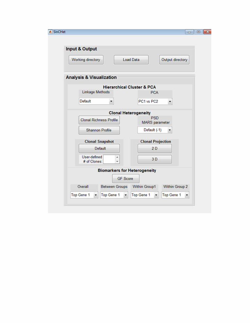

(2) Select the "Working directory" pushbutton and a window will display. You can choose the directory that contains source code of our SinCHet with MATLAB environment. This step is not necessary for people who use the pre-compiled PC versions.
(3) Select the "Load Data" pushbutton and a window will display. You can choose
the fold in your PC that contains the datasets to be analyzed. The datasets can be either Excel or MATLAB files. Datasets contain the header with group names at the first row, gene names at the first column and numerical matrix with n (genes) of rows by p (cells) of columns.
(4) Select the "Output directory" pushbutton and a window will display. You can
choose the fold in your PC where all analyzed results and plots are stored.
2. Analysis & Visualization
2.1 Hierarchical clustering and principal components analysis (PCA) (1) Select either the default or user-defined linkage method from the “Linkage
Methods” dropdown menu for hierarchical cluster analysis. The default linkage method is the linkage method with the highest calculated cophenetic correlation coefficient (Sokal, 1962). A dendrogram plot of hierarchical cluster tree with heatmap is displayed in a popup window for visualization. The figures below showed the gene expression results in the left panel and discretized methylation results in the right panel. All the figures in the following sections in this manual are also organized in the same order (i.e., left: expression; right: methylation)
• Sokal, R.R.a.R., F. J. (1962) The comparison of dendrograms by objective methods., Taxon, 11, 33-40.
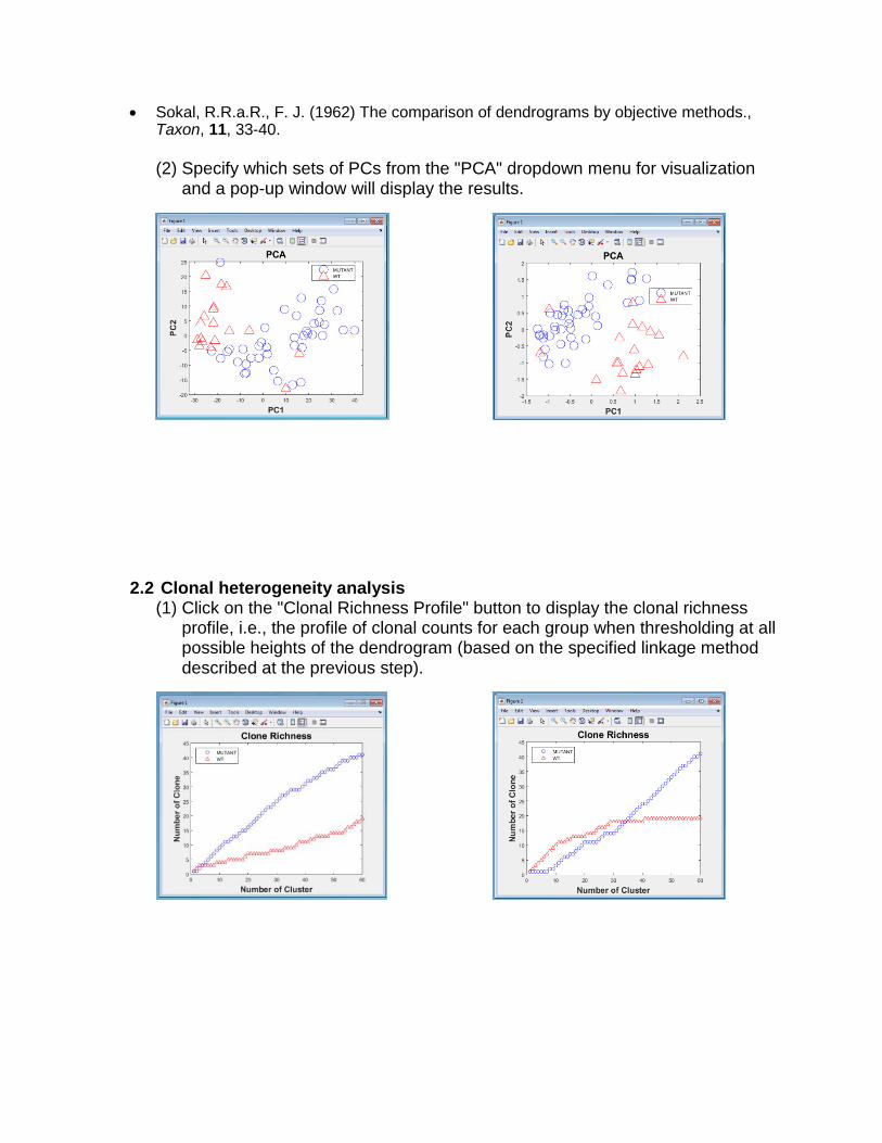
(2) Specify which sets of PCs from the "PCA" dropdown menu for visualization
and a pop-up window will display the results.
2.2 Clonal heterogeneity analysis (1) Click on the "Clonal Richness Profile" button to display the clonal richness
profile, i.e., the profile of clonal counts for each group when thresholding at all possible heights of the dendrogram (based on the specified linkage method described at the previous step).

(2) Click on the "Shannon Profile" button to display the Shannon Profile (SP) and quantify overall heterogeneity under each condition. The D statistic characterizing the heterogeneity differences between two groups will be estimated and displayed. Its associated p-value will be estimated using a permutation procedure. This step will take a while and a warning sign of “Waiting for estimation of p-value” is display during the permutation procedure.
(3) Select the parameter setting from the “PSD MARS parameter” dropdown menu to choose setting for the multivariate adaptive regression splines (MARS) model and display the detected change points for PSD. The original default of value for the MARS parameters of “useMinSpan” and

“useEndSpan" is -1, and set as the default here, too. It enables automatic mode that chooses value for this parameter (but not lower than 7). The choice of 0 or 1 setting disables the protection so that all the observations could be considered for knot placement. And “>1” setting (set as 2 in the current implementation) enables manual tuning of the value to be more responsive to local variations in the data (useful when the number of data observations is small) however this could also lead to overfitting (Jekabsons, 2016). It is a trade-off.
• Jekabsons, G. (2016) ARESLab: Adaptive Regression Splines toolbox for Matlab/Octave, available at http://www.cs.rtu.lv/jekabsons/
(4) In the "Clonal Snapshot" panel, click on the “Default” button to display clonal composition (i.e., the percentage of cells in each clone for each group in a pie chart) at the default clonal resolution. The default number of clones is the minimum value of the change points detected by MARS. Alternatively, the user can specify a desired number of clones by entering an integer between 1 and the total sample size. The clonal composition at the defined clone resolutions will be displayed. The analyses followed by the clonal snapshot, including clonal projection and biomarker analyses, will be performed based on the specified clonal resolution at this step.

(5) In “Clonal Projection” panel, select “2D” or “3D” from the dropdown menu to
visualize the clonal relationships at the defined clonal resolution as described above). The color codes for clones while size of the nodes coded for groups.

2.3 Biomarkers for heterogeneity (1) Click on the "GF Score" button to visualize the biomarkers results and save
the tests results in an excel file. The worksheet of “GF score” in the excel file contains the results from between- and within- condition comparisons, their p-values, FDR values and fold changes (or odds ratio) and overall GF score for each gene at the defined clonal resolution (as described above). In the pop-up window, a figure summarizing the heterogeneity evidence for each biomarker prioritized using the GF score (with the -log 10 (p value) displayed from each of the within- and between- condition comparisons along each axis). The names of the top three gene based on GF score will be displayed.

(2) Select one of the top 3 genes from the “Overall” dropdown menu for visualization using boxplots or bar charts (depending on the datatypes). The genes are ranked based on GF scores combining the evidences from three comparisons between and within conditions.
(3) Select one of the top 3 genes from the “Between Groups” dropdown menu for
visualization using a boxplot or bar chart conditions (depending on the datatypes). The genes are ranked based on p value derived from the comparison of the dominant clones between two conditions.
(4) Similarly, select one of the top 3 genes from either the “Within Group1” or “Within Group2” dropdown menu for visualization using a boxplot or bar chart. The genes are ranked based on p value derived from the comparison between the dominant clone and the other clones combined within each condition.

Note: All plots generated by the above processing are stored at the output directory with .jpg format. In addition, all plots can be saved as a different format such as .png, .tiff, etc. at the desired fold once the figures displayed.