Embed Size (px)
DESCRIPTION
This is the Workspace User's Guide for the SimXpert Structures Workspace.
Citation preview

1Introduction
Workspace User’s GuidesStructures Workspace GuideIntroduction

Overview of structures workspace2
Overview of structures workspaceSimXpert structures workspace is a very powerful yet easy to use general purpose finite element analysis (FEA) program to analyze structures. The term structure includes not just the traditional structures such as buildings, bridges, ships, airplanes, and automobiles, but also mechanical components such as machine parts and tools. Based on the widely used MD Nastran and Marc programs, the structures workspace can efficiently solve problems ranging from relatively simple linear statics to extremely complex and very large nonlinear and dynamic simulations.

3IntroductionCapabilities and supported solutions
Capabilities and supported solutionsSimXpert structures workspace includes ten analysis types (solution sequences or procedures). Each of these analysis types are discussed in detail in this guide. A brief description is given in this introduction.
Linear Static (Sol 101)The linear static module is used to calculate displacements, stresses, strains, etc. under static loading. It assumes that the stiffness of the structure does not change with the loading. It is generally valid when the displacements are small, stresses remain elastic, and with no change in contact status.
Modal Analysis (Sol 103)Modal analysis is used to compute the natural frequencies and the associated mode shapes of a structure.
Linear Buckling (Sol 105)The linear buckling module is used to calculate linear elastic buckling loads and mode shapes. It is generally valid when the displacements are small, stresses remain elastic, and with no change in contact status.
Direct Complex Eigenvalues (Sol 107)Used for the analysis of aeroelastic flutter, acoustics, rotating bodies, and many other physical effects. This solution will indicate the overall dynamic behavior dominated by the lowest frequency natural modes and resonant frequencies.
Direct Frequency Response (Sol 108)The direct frequency response analysis is used to calculate the steady state displacements, velocities, accelerations, stresses, strains, etc. under harmonically (e.g. sinusoidal) time-varying loads. It solves the dynamic equilibrium equation of motion by assuming that the steady state response to harmonic loads to be also harmonic.
Direct Transient Analysis (Sol 109)The direct transient dynamic analysis is used to calculate the displacements, velocities, accelerations, stresses, strains, etc. under time-varying loads. It solves the dynamic equilibrium equation of motion by direct numerical integration.
Modal Complex Eigenvalues (Sol 110)Used for the analysis of aeroelastic flutter, acoustics, rotating bodies, and many other physical effects.

Capabilities and supported solutions4
Modal Frequency Response (Sol 111)The modal frequency response analysis is used to calculate the steady state displacements, velocities, accelerations, stresses, strains, etc. under harmonically (sinusoidally) time-varying loads. It solves the dynamic equilibrium equation of motion by assuming that the steady state response to harmonic loads to be also harmonic. It solves the dynamic equilibrium equation of motion by first transforming it into the modal coordinates. By taking advantage of the fact that a relatively few normal modes can often adequately describe the motion of the structure, the modal frequency response method solves linear frequency response problems in a fraction of the time taken for the Direct modal frequency response method.
Modal Transient Analysis (Sol 112)Modal transient dynamic analysis is used to calculate the displacements, velocities, accelerations, stresses, strains, etc. under time-varying loads. It solves the dynamic equilibrium equation of motion by first transforming it into the modal coordinates. By taking advantage of the fact that a relatively few normal modes can often adequately describe the motion of the structure, the modal transient dynamics method solves linear transient dynamic problems for large models in a fraction of the time taken for the Direct transient method.
General Nonlinear (Sol 400)Analyzes a wide variety of structural problems subjected to geometric and material nonlinearities, and contact.
Implicit Nonlinear (Sol 600)Analyzes a wide variety of structural problems subjected to geometric and material nonlinearities, and contact.

5IntroductionTypes of elements used in structures workspace
Types of elements used in structures workspaceWorkspace structures supports a large number of elements ranging from simple rods, beams and springs to continuum hexahedrons and tetrahedrons for modeling any structural analysis problems. The full library of elements are listed below.
0D elements• CONM1 - a concentrated mass element (general form)
• CONM2 - a concentrated mass element (rigid body form)
• CElas -a scalar spring element
1D elements• CBAR - a simple beam element
• CBEAM - a beam (nonlinear) element
• CBEND- a curved beam or pipe element
• CBUSH -a a generalized spring and damper element
• CDAMP1 -a scalar damper element
• CDAMP1D -a scalar damper connection for use in the Crash workspace (Sol 700).
• CDAMP2 -a scalar damper element (alternative format of CDAMP1)
• CDAMP2D -a scalar damper connection for use in the Crash workspace (Sol 700).
• CELAS1 - a scalar spring connection element
• CELAS1D -a scalar spring connection for use in the Crash workspace (Sol 700).
• CELAS2 - a scalar spring element (alternative format of CELAS1)
• CELAS2D -a scalar spring connection for use in the Crash workspace (Sol 700).
• CGAP- a gap or friction element
• CMASS1 -a scalar mass element
• CMASS2 -a scalar mass element (alternative format of CMASS1)
• CONROD - a rod (tension-compression-torsion) element (alternative format of CROD)
• CROD - a rod (tension-compression-torsion) element
• CTUBE- a tube (tension-compression-torsion) element
• CVISC -a viscous damper element
• FEEDGE -Defines a finite element edge and associates it with a curve
• PLOTEL -A one-dimensional dummy element used for graphics purposes.

Types of elements used in structures workspace6
Plates and shell elements• CQUAD4 - a 4-noded quadrilateral shell element
• CQUADR -a 4-noded quadrilateral shell element with normal rotational degrees of freedom
• CSHEAR -a 4-noded quadrilateral shear panel element
• CTRIA3 - a 3-noded triangular shell element
• CTRIAR -a 3-noded triangular shell element with normal rotational degrees of freedom
• CTRIA6 - a 6-noded triangular shell element
• CQUAD8 -a 8-noded quadratic shell element
• RTRPLT -A rigid triangular plate
• CAABSF -A frequency dependent acoustic absorber element in coupled fluid-structural analysis
• CIFQUAD-a Sol (400) shell element used for simulating the progress of delamination with 4 or 8 nodes
All the above elements except CSHEAR are available for the analysis of plate and shell structures of homogeneous, laminated composite, and sandwich constructions.
2D solid elements• CTRIAX -a triangular axisymmetric solid element with up to 6 nodes
• CQUADX -a quadrilateral axisymmetric solid element with up to 9 nodes
• CIFQDX-a Sol (400) axisymmetric element used for simulating the progress of delamination with 4 or 8 nodes
3D solid elements• CHEXA - a a hexahedral solid element with 8 to 20 nodes
• CPENTA - a a pentahedral solid element with 6 to 15 nodes
• CTETRA - a a tetrahedral solid element with 4 to 10 nodes

7IntroductionTypes of materials used
Types of materials usedStructures workspace supports isotropic, orthotropic, and anisotropic material properties. Nonlinear elastic, elastic-plastic, and hyper-elastic material properties are supported for nonlinear analysis. Temperature dependent material properties are also allowed, for both linear and nonlinear analysis. The complete list of materials supported by structures workspace is given below.
Isotropic Materials (MAT1, MATT1)Defines the isotropic material properties such as Young’s modulus, Poisson’s ratio, Density, coefficient of thermal expansion, element damping coefficient, and optionally, the stress limits.
Orthotropic materials for shells (MAT8, MATT8)Defines the orthotropic material properties for shell elements.
Orthotropic materials for axisymmetric solid (MAT3, MATT3)Defines the orthotropic material properties for 2D solid elements.
Orthotropic materials for 3D solid and plane strain (MAT3, MATORT)Defines the orthotropic material properties for axisymmetric solid elements.
Anisotropic materials for shells (MAT2, MATT2)Defines the anisotropic material properties for shell elements.
Anisotropic materials for 3D solid (MAT9, MATT9)
Defines the anisotropic material properties for 3D solid elements.
Elasto-plastic material properties (MATEP, MATS1)Defines the elasto-plastic material properties
Failure properties (MATF)Defines the failure (strength) model properties for linear elastic materials.

Types of materials used8
Visco-plastic or creep material properties (MATVP)
Specifies visco-plastic or creep material properties.
Gasket material properties (MATG, MATTG)Defines the failure (strength) model properties for linear elastic materials.
Hyperelastic material properties (MATHE, MATHP)Defines hyperelastic material properties
Damage model properties for hyperelastic materials (MATHED)Defines hyperelastic material properties

9IntroductionOverview of typical steps used
Overview of typical steps usedThe procedure for performing any type of analysis with the structures workspace are essentially the same, and consist of the following steps:
The following procedure shows the general recommended workflow for the Structures, Thermal , Crash, and Explicit workspaces.
1. Designate a system of units
2. Import/create geometry
Or

Overview of typical steps used10
3. Create the finite element mesh
4. Create material and element properties
5. Apply loads and boundary conditions
6. Set up analysis

11IntroductionOverview of typical steps used
7. Submit model to solver

Overview of typical steps used12
8. Access results
9. Post-process

17Linear Statics
Linear Statics

Overview and Definition18
Overview and Definition
IntroductionLinear static analysis represents the most basic type of structural analysis. A “static” analysis is valid, if the structure is loaded gradually (i.e. at a rate much slower than the lowest fundamental period of the structure). It ignores inertia and damping effects. Some examples of valid static analyses are: analysis of structures subjected to slowly applied forces or prescribed displacements, spinning with a constant angular velocity, moving with constant acceleration, and thermal loading due to a slow change in the steady state temperature. A static analysis is invalid when the applied loading has one or more frequencies approaching any of the fundamental (resonant) frequencies of the structure.
TheoryThe static analysis solves the following equation:
where: F, K, and d are respectively the nodal forces, the model stiffness, and the nodal displacements.
The nodal forces are known (input), and the model stiffness is computed from the elements’ geometries and properties. In a linear static analysis, the stiffness [K] is assumed to remain constant, and consequently, the response of the structure (displacements, stresses, strains etc.) varies linearly with the applied forces. For example, a doubling of the applied forces would result in a doubling of the displacements, stresses, and strains in the structure. The assumption of linearity is usually valid, unless the structure experiences large deformations, or stresses beyond the elastic limit, or any change in contact conditions between one or more regions of the structure.
The applied forces may be used separately, or combined with each other to form load cases representing various scenarios or operating environments. Analyzing for multiple (loading) subcases in a single job (run) is very efficient, since the solution time for the second and subsequent subcases is a small fraction of the solution time for the first, especially if the boundary condition (constraint) does not change between the subcases.
Method of solutionThe equilibrium equation for linear statics, F = Kd, is solved either by a direct or an iterative solver, to compute the displacements. The iterative solver available in the Structures Workspace allows the efficient solution of very large models with hundreds of thousands of degrees of freedom. Strains, stresses, strain energies, element forces, and reaction forces are then computed using the nodal displacements.
F Kd=

19Linear StaticsParts and Geometry
Parts and GeometryThe geometry of the parts can be either created in SimXpert, or more likely imported from CAD program such as Catia, Pro/Engineer, or Unigraphics.
UnitsSimXpert interprets all dimensions and input data with respect to a system of units. It is important to set the appropriate units prior to importing any unitless analysis files (such as a Nastran Bulk Data file) or creating materials, properties, or loads. You can control the system of units by selecting Options > General > Units Manager from the Tools menu. If you import a file that contains units, SimXpert will convert them into those specified in the Units Manager.
Creating geometryIt is possible to create some geometry types in SimXpert. Complex geometry is often accessed or imported from an external source. All geometry can be edited in SimXpert
Importing geometryIf the geometry of the part or assembly is available in a CATIA v4, CATIA v5, Pro/Engineer, ACIS, parasolid, IGES, STEP, UGS NX or STL file, it can be imported into the SimXpert Structures Workspace.

Parts and Geometry20
Creating local coordinate systemsSometimes it is convenient to use local coordinate systems for specifying loads, and or boundary conditions. For example, a certain node may have a roller support placed in an inclined plane. A local coordinate system with one of its axes normal to the inclined plane needs to be created and used to specify the fixity (SPC) of the displacement component along the direction normal to the inclined plane.
Local coordinate systems can be in cartesian, cylindrical or spherical systems. Coordinate system created in SimXpert are represented by the following icons, corresponding to the method selected.
Coordinate System
Direction 1
Direction 2
Direction 3 1-3 plane
Cartesian x y z x-z (y=0)
Cylindrical r z r-z ( =0)
Spherical r r- ( =0)
CONSTRAINTCONSTRAINT
Cartesian
Cylindrical
Spherical
θ θθ φ φ θ

21Linear StaticsParts and Geometry
You can create local coordinate systems by selecting Cartesian, Cylindrical, or Spherical from the Coordinate System group under the Geometry tab. There are numerous methods to create local coordinate systems in SimXpert:
1. 3 Points: Three points are used to define the coordinate system. The first point corresponds to the location of origin. The second point defines the point on a specified axis and the third point defines a point in a specified plane.
2. Euler: Creates a coordinate system through three specified rotations about the axes of an existing coordinate system.
3. Normal: Creates a coordinate system with its origin at a point location on a surface. A specified axis is normal to the surface.
4. Two Vectors: Creates a coordinate system with its origin at a designated location and two of the coordinate frame axes are defined using vectors
5. Advanced: Location and orientation can be independently defined. There are 4 different ways to define the location of the origin of the coordinate system: Geometry, Point/Node, Coordinate System, and Center of Part. Further, the orientation can also be defined 3 ways: Global, Two Axes, and Coordinate System.
Example
To create a Cartesian coordinate system using 3 points method:
1. Select Coord > Cartesian from the Construction Geom group under the Geometry tab.
2. Pull down Method to 3 Points.
3. Select a Part to which the coordinate frame will belong. If no Part is selected, a default Part will be created.
4. Optionally, click in the Ref Sys text box and select a local coordinate system that will be used to define the three points. Leave this blank to use the basic coordinate system.
5. Location: Enter 10, 0, 0 to specify the point location for origin..
6. Point on Axis: Select X as the local axis that is being defined. Enter 10,1,0 to align the local X-axis with the global Y.

Parts and Geometry22
7. Point on Plane: Select XYas the local plane is being defined. Enter 9,1,0 to specify a point which lies in this plane.... .
8. Click OK to create the coordinate system.
Y
Z
X
First Point, a point locationfor origin
Second Point, a point on aspecified axis (X) Third Point, a point in a specified
plane XY

23Linear StaticsParts and Geometry
To create a Cylindrical coordinate system using Euler method:
1. Select Coord > Cylindrical from the Construction Geom group under the Geometry tab.
2. Pull down Method to Euler.
3. Select a Part to which the coordinate frame will belong.
4. Optionally, click in the Ref Sys text box and select a local coordinate system that will be used to define the new coordinate system. Leave this blank to use the basic coordinate system.
5. For Location, enter 0, 0, 0 to specify the point location for origin.
6. For Orientation, Select 3-1-3 for rotational sequence. This will perform rotations about the basic z-axis, then the new orientation of the x-axis, and finally the new orientation of the z-axis.
7. Enter (30, 30, 0) to specify the rotations about the axes.
8. Click OK to create the coordinate system.
To create a Spherical coordinate system using Normal method:
1. Select Coord > Spherical from the Construction Geom group under the Geometry tab.
2. Pull down Method to Normal..
3. Select a Part to which the coordinate frame will belong.
4. Optionally, click in the Ref Sys text box and select a local coordinate system that will be used to define the new coordinate system. Leave this blank to use the basic coordinate system.

Parts and Geometry24
5. For Location, select a node for the local origin.
6. Select a surface to which the z-axis of the coordinate system will be normal.
7. Select R Axis along Normal.
8. Select T along U direction.
9. Click OK to create the coordinate system.
To create a Cartesian coordinate system using Two Vectors method:
1. Select Coord > Cartesian from the Construction Geom group under the Geometry tab.
U
V
rp
t
Point/Node to define thelocation of origin

25Linear StaticsParts and Geometry
2. Pull down Method to Two Vectors.
3. Select a Part to which the coordinate frame will belong.
4. Optionally, click in the Ref Sys text box and select a local coordinate system that will be used to define the new coordinate system. Leave this blank to use the basic coordinate system.
5. For Location, enter 0,0,0 to define the origin.
6. In Vector for Axis-1, select X to define the local axis. Enter 0.5,0,0; 1,0,0 to define a vector along the specified axis as shown in figure below.

Parts and Geometry26
7. In Vector for Axis-2, select Y to define the local axis. Enter 0,1,0; 0,1,1 to define a vector along the specified axis as shown in figure below.
8. Click OK to create the coordinate system.
Y
Z
X
First, a point location for origin
Second, two points to define the Vector for Axis-1
Third, two points to define the Vector for Axis-2
(0, 0, 0) (0, 0.9, 0)(0.5, 0, 0)
(1, 0, 0)
(0, 1, 0)

27Linear StaticsParts and Geometry
You can assign a local coordinate system to a Nodal Location (reference LCS), Nodal Displacement (output LCS), or to shell elements by selecting Assign LCS from the Modify group under the Nodes/Elements tab.
Settings that affect the display of Local Coordinate Systems are
• Tools > Options, Workspaces > Structures > Entity Options: to control the LCS axis size, labels, color, and so on.
• Local Coordinate System display options can be individually controlled using the Visualization tab on the Coordinate System form. You can access this form for existing coordinate systems by double clicking the coordinate system name in the Model Browser.
• Entity Display Filter toolbar Show/Hide Local Coordinate Systems icon to control whether local coordinate systems are displayed in the window.

Materials28
MaterialsThe material definitions discussed in this chapter include:
• Isotropic material (MAT1 entry) -- An isotropic material property is defined as a material having the same properties in each direction. This material may be used with all linear elements.
• Two-dimensional anisotropic material (MAT2 entry) -- Material definition for plate and shell elements. Anisotropic materials have properties that vary with direction and have no planes of symmetry. The in-plane material properties are defined with respect to an element material coordinate system. Transverse shear material properties may be included.
• Axisymmetric solid orthotropic material (MAT3 entry) -- A three-dimensional material property for axisymmetric analysis only. An Orthotropic material has properties which vary with direction. The elastic properties are specified in three orthogonal directions.For an Orthotropic material three Young's moduli are required - E1, E2 and Ez - where the out-of-plane elastic modulus Ez is no longer equal to E1. Three separate Poisson’s ratios are also required, n12, n1z and n2z, as is the in-plane shear modulus G12.
• Two-dimensional orthotropic material (MAT8 entry) -- Defines an orthotropic material property for plate and shell elements. Transverse shear material properties may also be included. Some engineering materials, including certain piezoelectric materials and 2-ply fiber-reinforced composites, are orthotropic. By definition, an orthotropic material has at least 2 orthogonal planes of symmetry.
• Three-dimensional anisotropic material (MAT9 entry) -- Defines an anisotropic material property of solid elements. The MAT9 entry may also be used to define a three-dimensional orthotropic material.
Defining Mass in Your ModelCommon ways to define mass are the concentrated masses (CMASSi and CONMi), mass density on the material entries, and nonstructural mass defined on the property entries. The mass density defined on the material entries is given in terms of mass/unit volume. You must be sure the mass unit is consistent with the other units in the model. For example, in the English system (in, lb., sec.), the mass density of steel
is approximately .
The nonstructural mass defined on the property entries is mass that is added to the structure in addition to the structural mass from the elements. For one-dimensional elements, the units are mass/unit length. For two-dimensional and three-dimensional elements, the units are mass/unit area and mass/unit volume, respectively.
It is often convenient to express the mass in terms of weight units instead of mass units. This can be accomplished with the use of the solution parameter Weight - Mass Conversion. The function of the Weight - Mass Conversion factor is to multiply the assembled mass matrix by the scale factor entered.
For the steel example, the mass density can be entered as a weight density of with a Weight - Mass Conversion value of 0.00259 (which is 1/386.4). As a word of caution: if you enter any
7.32 104– lb-sec
2in
4⁄⋅
0.283 lb in3⁄

29Linear StaticsMaterials
of the mass in terms of weight, you must enter all the mass in terms of weight. The Weight - Mass Conversion factor multiplies all of the mass in the model by the same scale factor. There are two ways to enter this parameter in SimXpert. One method is to select PARAM from the ASSEMBLE tab. The parameter name used here is WTMASS. In the Parameter value 1 field you enter the weight to mass conversion factor.
The second method to enter this parameter is discussed in Weight - Mass Conversion.
Supported Materials
Isotropic Material
The isotropic material, defined by the MAT1 Nastran entry, is the most commonly used material property. An isotropic material is defined as having the same properties in any direction. Furthermore, the isotropic material is fully described by only two material constants. These two constants may be any combination
of E, G, and . You may specify all three of these constants if desired, but remember, it only takes two of the constants to define the material. When you enter only two constants, the third is computed from the following relationship:
(2-1)
where:
E = Young’s Modulus
G = Shear Modulus, and
= Poisson’s Ratio
The isotropic entry may also be used to define such things as
ν
GE
2 1 ν+( )--------------------=
ν

Materials30
• Mass density (Density)
• The mass properties are only required in static analysis when a gravity loading or rotating force is used; however, they are useful for model verification with any loading condition.
• Coefficient of thermal expansion (Thermal Exp. Coeff.)
• Structural element damping (Struct. Elem. Damp. Coeff.)
• Failure limits
• Tension Stress Limit
• Compression Stress Limit
• Shear Stress Limit
Stress limits are used to compute margins of safety for certain line elements only.
The input for Isotropic material (MAT1 entry) appears as follows:.

31Linear StaticsMaterials
To access additional choices click Advanced:
Other choices are available under the Isotropic material form. They are
• Thermal
• Stress Dependent
• Elasto Plastic
• Visco Elastic
• Visco Plastic
• Creep
• Failure

Materials32
These are accessed through tabs that can be displayed by clicking the Add Constitutive Model button.
By selecting the desired tabs; i.e. Stress Dependent, Failure; the material model can be modified. A constitutive model can be eliminated by clicking the Delete Model button.
Anisotropic 2D
The anisotropic 2D references a MAT2 Nastran card. The anisotropic two-dimensional entry defines a stress-strain relationship of the form shown in Equation (2-2) and Equation (2-3). This entry can only be
used with plate and shell elements. The reference temperature is given by and the thermal
expansion coefficients are A1, A2, and A3. The component directions X and Y refer to the element material coordinate system, which is explicitly defined for each element. The material coordinate system for the CQUAD4 element is shown in Figure 2-1. The in-plane stress-strain relationship is described by Equation (2-2). Equation (2-3) defines the transverse shear stress - transverse shear strain relationship.
TREF

33Linear StaticsMaterials
(2-2)
(2-3)
σx
σy
τxy
G11 G12 G13
G12 G22 G23
G13 G23 G33
εx
εy
γxy
T TREF–( )A1
A2
A3
–
=
τxz
τyz
G11 G12
G12 G22
γxz
γyz
=

Materials34
The input for Anisotropic 2D appears as follows:
Orthotropic 2D Axisymmetric
The orthotropic two-dimensional axisymmetry entry defines a relationship in a cross sectional coordinate
system (x, , z). You can only use the material property with the axisymmetric CTRIAX6 element. The axisymmetric solid orthotropic material is defined by Equation (2-4).
θ

35Linear StaticsMaterials
(2-4)
To preserve symmetry, the following relationships must hold:
(2-5)
εx
εθ
εz
γzx
1Ex-----
νθx–
Eθ-----------
νzx–
Ez---------- 0
νxθ–
Ex----------- 1
Eθ------
νzθ–
Ez---------- 0
νxz–
Ex----------
νθz–
Eθ---------- 1
Ez----- 0
0 0 01
Gzx--------
σx
σθ
σz
τzx
T TREF–( )
Ax
Aθ
Az
0
+=
νxθEx-------
νθx
Eθ-------
νxz
Ex-------
νzx
Ez-------
νθz
Eθ-------
νzθEz-------=;=;=

Materials36
The input for Orthotropic 2D Axi appears as follows:
Orthotropic 2D
The two-dimensional orthotropic entry defines a stress-strain relationship as shown in Equation (2-6) and Equation (2-7). This entry can only be used with the plate and shell elements. Equation (2-6) defines the in-plane stress-strain relationship. The transverse shear stress-transverse shear strain relationship is defined by Equation (2-7)

37Linear StaticsMaterials
. (2-6)
(2-7)
ε1
ε2
γ12
1E1------
ν12–
E1----------- 0
ν12–
E1----------- 1
E2------ 0
0 01
G12---------
σ1
σ2
τ12
T TREF–( )A1
A2
0
+=
τ1z
τ2z
G1z 0
0 G2z
γ1z
γ2z
=

Materials38
The input for Orthotropic 2D appears as follows:
Anisotropic 3D
The anisotropic entry defines a material property for the CHEXA, CPENTA, and CTETRA solid elements. The three-dimensional anisotropic material is defined by Equation (2-8)

39Linear StaticsMaterials
. (2-8)
σx
σy
σz
τxy
τyz
τzx G11 G12 G13 G14 G15 G16
G12 G22 G23 G24 G25 G26
G13 G23 G33 G34 G35 G36
G14 G24 G34 G44 G45 G46
G15 G25 G35 G45 G55 G56
G16 G26 G36 G46 G56 G66
εx
εy
εz
γxy
γyz
γzx
T TREF–( )
A1
A2
A3
A4
A5
A6
–
=

Materials40
The input for Anisotropic 3D appears as follows:
Required Material PropertiesYou must define stiffness in some form (for example, Young's modulus (E), Shear Modulus (G), or hyperelastic coefficients).

41Linear StaticsMaterials
For Global Boundary Conditions (such as gravity or rotating force), you must define the data required for mass calculations, such as density (RHO).
For thermal loads (temperatures), you must define the coefficient of thermal expansion (A).

Element Properties42
Element Properties
OverviewTypical properties include cross-sectional properties of beam elements, thicknesses of plate and shell elements, material IDs, etc. Properties are assigned to the elements of a specified part or element type, either directly to the elements, or indirectly through the part to which the elements belong or the geometry with which the elements are associated.
Properties associate materials with elements.
Element types and associated properties
Two-Dimensional Elements
Two-dimensional elements, commonly referred to as plate and shell elements, are used to represent areas in your model where one of the dimensions is small in comparison to the other two.
• CQUAD4, CTRIA3 - General-purpose plate elements capable of carrying in plane force, bending forces, and transverse shear force. This family of elements are the most commonly used 2-D elements in the SimXpert element library. These are the element types generated by the Automesher.
• CSHEAR - A shear panel element, i.e., the element can transmit in plane shear forces only.
• CQUAD8, CTRIA6 - Higher order elements that are useful for modeling curved surfaces with fewer elements than are required if you use the CQUAD4 and CTRIA3 elements. In general, the CQUAD4 and CTRIA3 elements are preferred over the CQUAD8 and CTRIA6 elements.
• CQUADR and CTRIAR - This family of 2-D elements are complementary to the CQUAD4 and CTRIA3 elements.
• The CTRIAX6 - An axisymmetric solid of revolution element. This element is used only in axisymmetric analysis.
PSHELL
The CQUAD4, CTRIA3, CQUAD8, CTRIA6, CQUADR, and CTRIAR elements are commonly referred to as the plate and shell elements within SimXpert. Their properties, which are defined using the PSHELL entry, are identical. For all applications other than composites or shear panels, the PSHELL entry should be used for plate and shell elements.

43Linear StaticsElement Properties
The format of the Shell Property entry is as follows:
As can be seen, the Shell entry is used to select the material for the membrane properties, the bending properties, the transverse shear properties, the bending-membrane coupling properties, and the bending and transverse shear parameters. By choosing the appropriate materials and parameters, virtually any plate configuration may be obtained.
The most common use of the Shell entry is to model an isotropic thin plate. The preferred method to define an isotropic plate is to select an isotropic material for the Material (membrane Material ) on the basic form entry of the Shell properties form and Bending material ID on the advanced portion of the form. For a thick plate, you may also wish to enter an isotropic material for the Transverse shear material .
Also located on the Shell entry are the stress recovery locations Z1 and Z2, located under Fiber distance for stress computation on the advanced portion of the form. By default, Z1 and Z2 are equal to one-half of the plate thickness (typical for a homogeneous plate). If you are modeling a composite plate, you may wish to enter values other than the defaults to identify the outermost fiber locations of the plate for stress analysis.

Element Properties44
The element coordinate systems for the CQUAD4 is shown in Figure 2-1. The orientation of the element coordinate system is determined by the order of the connectivity for the nodes. The element z-axis, often referred to as the positive normal, is determined using the right-hand rule (the z-axis is “out of the screen” as shown in Figure 2-1. Therefore, if you change the order of the nodal connectivity, the direction of this positive normal also reverses. This rule is important to remember when applying pressure loads or viewing the untransformed element forces or stresses. Untransformed directional element stress plots may appear strange when they are displayed by the postprocessor in SimXpert because the normals of the adjacent elements may be inconsistent. Remember that components of forces, moments, and element stresses are always output in the element coordinate system.
Figure 2-1 CQUAD4 Element Geometry and Coordinate Systems
PSHEAR
The CSHEAR element is a quadrilateral element with four nodes. The element models a thin buckled plate. It supports shear stress in its interior and also extensional force between adjacent nodes. Typically you use the CSHEAR element in situations where the bending stiffness and axial membrane stiffness of the plate is negligible. The use of CQUAD4 element in such situations results in an overly stiff model.
The most important application of the CSHEAR element is in the analysis of thin reinforced plates and shells, such as thin aircraft skin panels. In such applications, reinforcing rods (or beams) carry the extensional load, and the CSHEAR element carries the in-plane shear. This is particularly true if the real
N3
N4
N1 N2
THETA
yelement
xelement
xmaterialzelement
α β γ+2
------------=
α
βγ

45Linear StaticsElement Properties
panel is buckled or if it is curved. The properties of the CSHEAR element are entered on the Shear entry. The format of the Shear Property entry is as follows:
The optional stiffness factors are useful in representing an effective stiffness of the panel for extensional loads by means of equivalent rods on the perimeter of the element. If the stiffness factor for extensional stiffness G1-G2 and G3-G4 is less than or equal to 1.01, the areas of the rods on edges 1-2 and 3-4 are
set equal to where is the average width of the panel. If it is equal to 1.0, the panel
is fully effective in the 1-2 direction. If it is greater than 1.01, the areas for the rods on edge 1-2 and edge
3-4 are each set equal to . The significance of the stiffness factor for G2-G3 and G1-G4 for edges 2-3 and 1-4 is similar.
0.5 F1 T w1⋅ ⋅⋅ w1
0.5 F1 T2⋅⋅
Xelem
G4
G3
G2G1
Yelem

Element Properties46
Figure 2-2 CSHEAR Element Connection and Coordinate System
Figure 2-3 CSHEAR Element Corner Forces and Shear Flows
The Composite Element (PCOMP)
SimXpert provides a property definition specifically for performing composite analysis. You specify the material properties and orientation for each of the layers and SimXpert produces the equivalent PSHELL and MAT2 entries. Additional stress and strain output is generated for each layer and between the layers.
N4 N3
N2
N1
F43
K4 F41
F32
F34
F21
F23
K3
q3
q2
q1
q4
F14
F12
K2K1

47Linear StaticsElement Properties
The format of the Laminate Composite entry is as follows:
The following are the choices for laminate options:
• “Blank”All plies must be specified and all stiffness terms are developed.
• “SYM”Only plies on one side of the element centerline are specified. Computes the complete stiffness properties while specifying half the plies. The plies are numbered starting with 0 for the bottom layer. If an odd number of plies are desired, the center ply thickness (T1) should be half the actual thickness.
• “MEM”All plies must be specified, but only membrane terms are computed.
• “BEND”All plies must be specified, but only bending terms are computed.
• “SMEAR”All plies must be specified, ignores stacking sequence and is intended for cases where this sequence is not yet known, stiffness properties are smeared.
• “SMCORE” Allows simplified modeling of a sandwich panel with equal face sheets and a central core.All plies must be specified, with the last ply specifying core properties and the previous plies specifying face sheet properties. The stiffness matrix is computed by placing half the face sheet thicknesses above the core and the other half below with the result that the laminate is symmetric about the mid-plane of the core. Stacking sequence is ignored in calculating the face sheet stiffness.

Element Properties48
A two-dimensional composite material is defined as a stacked group of laminae arranged to form a flat or curved plate or shell. Each lamina may be considered as a group of unidirectional fibers. The principal material axes for the lamina are parallel and perpendicular to the fiber directions. The principal directions are referred to as “longitudinal” or the 1-direction of the fiber and as “transverse” or the 2-direction for the perpendicular direction (matrix direction).
A laminate is a stack of these individual lamina arranged with the principal directions of each lamina oriented in a particular direction as shown in Figure 2-4.
Figure 2-4 Laminae Arranged to Form a Laminate
The laminae are bonded together with a thin layer of bonding material that is considered to be of zero thickness. Each lamina can be modeled as an isotropic material (MAT1), two-dimensional anisotropic material (MAT2), or orthotropic material (MAT8). The assumptions inherent in the lamination theory are as follows:
• Each lamina is in a state of plane stress.
Xmat1( )
Xmat3( )
Ymat3( )
Xmat2( )
Ymat2( )Ymat
1( )

49Linear StaticsElement Properties
• The bonding is perfect.
• Two-dimensional plate theory can be used.
The output you may request for a composite analysis includes:
• Stresses and strains for the equivalent plate.
• Force resultants.
• Stresses and/or strains in the individual laminate including approximate interlaminar shear stresses in the bonding material output.
• A failure index table.
If you want stress and/or the failure indices for the composite elements, you must create an Output Request for Element Stresses. You will also want to specify the Composite Plate Option to request output at each individual ply or for the equivalent plate. Also, if you want the failure index table, you must enter
the stress limits for each lamina on the appropriate material entry, the shear stress limit , and the failure theory method on the Layered Composite form.
As an example of a layered composite, consider the cantilevered honeycomb plate shown in Figure 2-5. Although the honeycomb structure is not considered a composite layup, it can be analyzed effectively using a layered composite.

Element Properties50
Figure 2-5 Honeycomb Cantilever Plate
The material properties of the honeycomb section are given in Table 2-1.
10 in
2000 lb.
1000 lb.
1000 lb.30 in
Z
Y
X
Fixed Edge
t=0.42 inE=30 x 106 psi
Top Aluminum Face Sheet - T = 0.02 in
Honeycomb Core - T = 0.35 in
Lower Aluminum Face Sheet - T = 0.05 in
Table 2-1 Honeycomb Material Properties
Material
Modulus ofElasticity(106 psi)
TensileLimit
(103 psi)CompressionLimit (103 psi)
ShearLimit
(103 psi)
Aluminum Face Sheets
10.0 35 35 23
Core 0.0001 0.05 0.3 0.2
Bonding Material -- -- -- 0.1

51Linear StaticsElement Properties
Following are the corresponding MAT1 entries for the face sheets and the core respectively:

Element Properties52

53Linear StaticsElement Properties
To create the layup for the honeycomb plate we change the number of plies to 3 and input the data as follows:
Three-dimensional Elements
Whenever you need to model a structure that does not behave as a bar or plate structure under the applied loads, you need to use one or more of the three-dimensional elements. The three-dimensional elements are commonly referred to as solid elements. Typical engineering applications of solid elements include engine blocks, brackets, and gears.
Three-dimensional elements that are discussed in this chapter include
• CHEXA, CPENTA, and CTETRA - General-purpose solid elements. This family of elements is recommended for most solid model applications.

Element Properties54
PSOLID
The properties of Hexa, Penta, and Tetra type elements are entered on the SOLID form. The format of the SOLID entry is as follows:
One-Dimensional Elements
A one-dimensional element is one in which the properties of the element are defined along a line or curve. It has directional, end A is defined by the first node selected and end B by the second. Typical applications for the one-dimensional element include truss structures, beams, and stiffeners. One-dimensional elements discussed in this chapter include
• CROD - An element with axial stiffness and torsional stiffness about the axis for the element.
• CBAR - A straight prismatic element with axial, bending, and torsional stiffness.
• CBEAM - An element similar to the CBAR but with additional properties, such as variable cross-section, shear center offset from the neutral axis.
• CBEND - A curved element capable of internal pressure.
The CBAR Element
The CBAR element is a straight one-dimensional element that connects two nodes. The capabilities and limitations of the CBAR element are as summarized below:

55Linear StaticsElement Properties
• Extensional stiffness along the neutral axis and torsional stiffness about the neutral axis may be defined.
• Bending and transverse shear stiffness can be defined in the two perpendicular directions to the CBAR element’s axial direction.
• The properties must be constant along the length of the CBAR element. This limitation is not present in the CBEAM element.
• The shear center and the neutral axis must coincide. This limitation is not present in the CBEAM element.
• The ends of the CBAR element may be offset from the nodes.
• The effect of out-of-plane cross-sectional warping is neglected. This limitation is not present in the CBEAM element.
• Transverse shear stiffness along the length of the CBAR can be included.
The stiffness of the CBAR element is derived from classical beam theory (plane cross sections remain plane during deformation).

Element Properties56
The connectivity of the CBAR element is determined by the order in which you pick its two nodes. To create individual CBARs, select Bar from the 1D Elements group under the Nodes/Elements tab. The input form appears as follows:
Field Contents
Element Topology• Lower Order - To create simple beam and general beam element
• Higher Order - To create three-noded beam element
Element Type• Simple Bar - To create CBAR element
• General Beam - To create CBEAM element
Property Select or create a Beam property
Orientation Method
• Vector - Orientation vector will be specified by vector components.
• Node - The direction of the vector is from the starting node of the CBAR to the selected node. The vector is then translated to the starting end of the bar.
Functional FieldIf checked, a varying orientation vector will be defined by a previously created vector field.

57Linear StaticsElement Properties
Coordinate System
• Basic - Orientation components are with respect to the basic coordinate system
• Reference - Orientation components are with respect to the selected coordinate system.
Pick coordinate systemIf the Coordinate System Type is set to Reference, select the local coordinate system to be used to specify the orientation components.
Orientation components X, Y, Z
Components of orientation vector from the starting end of the bar.
Advanced Entries
OffsetsIf checked, vectors can be defined to offset the bar element from the nodes that define it.
End A / End B
Functional FieldIf checked, a variable offset vector will be defined by a previously created vector field.
Coordinate System
Coordinate system type for the offset vector at end A.
• Basic - Offset components are with respect to the basic coordinate system
• Offset - Offset components are measured with respect to the element coordinate system
• Reference - Offset components are with respect to the selected coordinate system.
Pick Coordinate SystemSelect a local coordinate system for offset vector at end A This option is available only if Reference Coordinate System is selected.
Offset Component Components of offset vectors (see Note 1)
Pin Flag
Pin flags for bar ends A and B, respectively. used to remove connections between the node and selected degrees of freedom of the bar. The degrees of freedom are defined in the element’s coordinate system (see Figure 2-9). The bar must have stiffness associated with the PA and PB degrees of freedom to be released by the pin flags. For example, if PA = 4, the PBAR entry must have a nonzero value for J, the torsional stiffness. (Valid input for this field: up to five of the unique integers 1 through 6 with no embedded blanks).
End ACheck the boxes for those degrees of freedom to be released at the starting node.
End BCheck the boxes for those degrees of freedom to be released at the ending node.
Field Contents

Element Properties58
BAR Property
The properties of the CBAR elements are entered on the Beam form. The format of the Beam property for the Bar element is as follows:
Any of the stiffnesses and flexibilities may be omitted by leaving the appropriate fields on the Beam entry blank. For example, if fields Inertia along ZZ and Inertia along YY are blank, the element will lack bending stiffness.
One the most difficult aspects of the CBAR (or CBEAM element) for the first-time users is understanding the need to define an orientation vector. The best way to see the need for the orientation vector is by an example. Consider the two I-beams shown in Figure 2-6. The I-beams have the same properties because they have the same dimensions; however, since they have different orientations in space, their stiffness contribution to the structure is different. Therefore, simply specifying the I-beam properties and the

59Linear StaticsElement Properties
location of the end points via the nodes is insufficient-you must also describe the orientation. This is done using the orientation vector.
Figure 2-6 Demonstration of Beam Orientation
Another way of looking at the orientation vector is that it is a vector that specifies the local element coordinate system. The orientation vector as it is related to the CBAR element coordinate system is
shown in Figure 2-7. Vector defines plane 1, which contains the elemental x- and y-axes.
Figure 2-7 CBAR Element Geometry without Offsets
Referring to Figure 2-7, the element x-axis is defined as the line extending from end A (the end at node NA) to end B (the end at node NB). Nodes NA and NB are defined on the CBAR entry. The element y-axis is defined to be the axis in Plane 1 extending from end A and perpendicular to the element x-axis. It is your responsibility to define Plane 1. Plane 1 is the plane containing the element x-axis and the orientation vector. After defining the element x- and y-axes, the element z-axis is obtained using the
right-hand rule, . Plane 2 is the plane containing element x- and z-axes. Note that once you define nodes NA and NB and the orientation vector, the element coordinate system is computed automatically by SimXpert.
x x
zz
x x
zz
v
End a
End b
Plane 2
Plane 1
NB
NA
v
yelem
zelem
xelem
z x y⊗=

Element Properties60
The vector shown in Figure 2-7 be may defined by one of two methods on the CBAR entry. One method is to define vector by entering the components of the vector, (X1, X2, X3), which is defined in a coordinate system located at the end of the CBAR. This coordinate system is parallel to the output coordinate system of the node NA. By default this is the basic coordinate system. You can assign a local coordinate system (output LCS) to nodes by selecting Assign from the Coordinate System toolbox. You can alternatively define the vector with the use of another node called G0, which is entered on the CBAR entry.
An additional feature of the CBAR element is the ability to remove some of the connections of individual degrees of freedom from the nodes. This operation is accomplished using the pin flags feature located on the CBAR entry (PA and PB). For example, suppose you want to connect two bar elements together with a hinge (or pin joint) as shown in Figure 4-19. To do this you will need to release the three rotational degrees of freedom. Therefore you can make this connection by entering DOFs 456 in the PB field of the CBAR entry.
Figure 2-8 Pin Flags for a Hinge Connection
Also note that the ends of the CBAR element may be offset from the grid points using ZA and ZB as defined on the CBAR entry. Therefore, the element x-axis does not necessarily extend from node NA to node NB; it extends from end A to end B.
Figure 2-9 CBAR Element Coordinate System with Offsets
Node NB
End a
End b
Plane 2
Plane 1
Node NA
v G0 )(
v
zb
za
zelem
yelem
xelem

61Linear StaticsElement Properties
If the CBAR is offset from the nodes and the components of the orientation vector are entered, then the tail of vector is at end A, not node NA. If the vector is defined with the use of a node G0, then it is defined as the line originating at node NA, not end A, and passing through G0. Note that Plane 1 is parallel to the vector NA-G0 and passes through the location of end A.
The offsets values ZA and ZB are entered by specifying the components of an offset vector in the output coordinate systems for NA and NB, respectively. The three components of each of the offset vectors are input using the CBAR entry. When you specify an offset, you are effectively defining a rigid connection from the grid point to the end of the element.
The element forces and stresses are computed and output in the element coordinate system. Figure 4-10 shows the forces acting on the CBAR element. V1 and M1 are the shear force and bending moment acting in Plane 1, and V2 and M2 are the shear force and bending moment acting in Plane 2.
Figure 2-10 CBAR Element Internal Forces and Moments (x-y plane)
Figure 2-11 CBAR Element Internal Forces and Moments (x-z plane)
The area moments of inertia I1 and I2 are input on the PBAR entry. I1 is the area moment of inertia to resist a moment in Plane 1. I1 is not the moment of inertia about Plane 1 as many new users may think at first. Consider the cross-section shown in Figure 2-10 and Figure 2-11; in this case, I1 is what most textbooks call Izz, and I2 is Iyy.
The area product of inertia I12, if needed, may be input on the PBAR entry. For most common engineering cross sections, it is usually not necessary to define an I12. By aligning the element y- and the z-axes with the principal axes of the cross section, I12, is equal to zero and is therefore not needed.
Plane 1a b
y
Tx
T
M1b
v1
v1
M1a
Fx
Plane 2
z
x
M2aM2b
v2
v2

Element Properties62
Stress recovery locations correspond to the locations C, D, E, and F on the PBAR entry. The location of these stress recovery coefficients are defined in CBAR’s element coordinate system. Consider the cross section for a 4mm X 2 mm bar as shown in Figure 2-12. On the PBAR entry you would input 2.0 for C1 and 1.0 for C2, -2.0 for D1 and 1.0 for D2, and so on for points E and F. By request, the stresses are computed at those four locations. As is commonly done, the stress locations represent the farthest points from the neutral axis of the cross-section. These points are the locations of the maximum bending stress.
Figure 2-12 Stress Recovery Locations
General Beam Library
General Beam Librayr provides an alternative and convenient method for defining bar cross sections. The Bar input that has been discussed so far requires you to calculate the cross-sectional properties of the beam (such as area, moments of inertia, shear center, etc.). Although this is not a particularly difficult task for standard cross sections, it is tedious and prone to unnecessary input errors.
A library is available to provide you with a simple interface to input beam cross sections into SimXpert. A number of common cross section types such as bar, box, I-beam, channel, angle, etc. can be described by the cross section’s dimensions instead of the section properties. For example, a rectangle cross section may be defined by its height and depth rather than the area, moments of inertia, etc. The section properties are calculated based on thin wall assumptions.
The Library entry allows you to input cross section types along with their characteristic dimensions. You can choose from 20 different cross section shapes. These shapes are as follows: ROD, TUBE, I, CHAN (channel), T, BOX, BAR (rectangle), CROSS, H, T1, I1, CHAN1, Z, CHAN2, T2, BOX1, HEXA (hexagon), HAT and HAT1(hat sections), and DBOX. For some of these shapes (I, CHAN, T, and BOX), you can select different orientations. All the shapes supported by SimXpert and their respective orientations and dimensions are shown in Figure 2-13.

63Linear StaticsElement Properties
To define section attributes such as height and width, use the Beam entry and select General as the Beam Type and Library as the Cross-section Type. To define section properties such as area and moment of inertia, use the Simple Cross-section type entry. The Library entries are easier to use and still retain most of the capabilities of the existing Simple method, including non-structural mass.
An additional difference between the Library and the Simple entries is that stress recovery points need not be specified to obtain stress output for the Library entry. The stress recovery points are automatically calculated at the extreme fibers to give the maximum stress for the cross section.
This automatic cross section computation greatly simplifies the formulation of design variables for design optimization applications

Element Properties64
DIM1
C
DF
E
DIM1
TYPE=“ROD”
DIM6
DIM4
CF
E D
TYPE=“I”
DIM5
C
DF
E
DIM1
TYPE=“TUBE”
DIM2
F
D
DIM4
DIM3
C
E
TYPE=“CHAN”
yelem
zelem
yelem
zelem
yelem
zelem
yelem
zelem
DIM3
DIM1 DIM2
DIM2
TYPE=“T”
yelem
zelem
DIM2
DIM1
DIM3
DIM4
F C D
E
TYPE=“BOX”
yelem
zelem
DIM3
DIM2
DIM1DIM4
C
DE
F
TYPE=“TUBE2”
C
DF
E
DIM1
DIM2
yelem
zelem

65Linear StaticsElement Properties
DIM4
TYPE=”BAR”
0.5 DIM1Þ
yelem
zelem
yelem
zelem
yelem
zelem
DIM2
C
DE
F
DIM1
DIM4
C
D
E
F
0.5 DIM1Þ
DIM3
DIM2
TYPE=”CROSS” TYPE=”H”
C
DE
F
DIM3
DIM1
0.5 DIM2Þ 0.5 DIM2Þ
yelem
zelem
DIM2DIM1
DIM3
DIM4 EC
D
F
TYPE=”T1”
0.5 DIM1Þ0.5 DIM1Þ
F C
E D
DIM2
DIM4
DIM3
TYPE=”I1”

Element Properties66
DIM4
DIM1DIM2
DIM3
DIM4
yelem
zelemDIM4
DIM3
DIM2 DIM1
E
F C
D
TYPE=”CHAN1”
DIM1 DIM1
yelem
zelem
DIM2
DIM3
D
C
TYPE=”CHAN2”
F
E
zelem
yelem
TYPE=”Z”
D
F C
E
yelem
zelem
DIM1
DIM2
DIM4C
DE
F
DIM3
TYPE=”T2”
DIM4
DIM3
yelem
zelemDIM2
DIM1
DIM6 DIM5
F C
DE
TYPE=”BOX1”

67Linear StaticsElement Properties
Figure 2-13 Cross-Section Geometry and Stress Recovery Points for PBARL
yelem
zelem
DIM1
DIM3
DIM1 DIM2
DIM3
DIM4
yelem
zelemC
E
D
F
DIM4
C
DE
F
TYPE=”HEXA” TYPE=”HAT”
DIM1
DIM2DIM4
C D
E F
TYPE=”HAT1”
DIM5
yelem
zelem
DIM3
DIM1DIM3
DIM7
DIM8
DIM12
DIM10
DIM9
DIM6DIM4
DIM5
TYPE = “DBOX”

Element Properties68
The input for the General Beam Library appears as follows:

69Linear StaticsElement Properties
The CBEAM Element
The CBEAM element provides all of the capabilities of the CBAR element discussed in the previous section, plus the following additional capabilities:
• Different cross-sectional properties may be defined at both ends and at as many as nine intermediate locations along the length of the beam.
• The neutral axis and shear center do not need to coincide. The feature is important for non symmetric sections.
• The effect of cross-sectional warping on torsional stiffness is included.
• The effect of taper on transverse shear stiffness (shear relief) is included.
• A separate axis for the center of nonstructural mass may be included.
The input as shown below for the CBEAM entry, is identical to that of the CBAR with the exception that you select General Beam for the Element Type

Element Properties70
Beam
The properties of the CBEAM elements are entered on the Beam form. The format of the Beam property for the Beam element is as follows:
The coordinate system for the CBEAM element, shown in Figure 2-14, is similar to that of the CBAR element. The only difference is that the element x-axis for the CBEAM element is along the shear center of the CBEAM. The neutral axis and the nonstructural mass axis may be offset from the elemental x-axis.

71Linear StaticsElement Properties
(For the CBAR element, all three are coincident with the x-axis.) The orientation vector is defined in the same manner as it is for the CBAR element.
Figure 2-14 CBEAM Element Geometry System
The CBEAM element presents you with more options than any other element in the SimXpert element library. It is not expected that you will employ all of the features of the CBEAM element at the same time. Therefore, you may omit most of the data fields corresponding to the features that are not being used. For those data fields that are left blank, a default value is used.
An exception to this rule is the data fields for A, I1, and I2. If any of these fields is left blank, a fatal message occurs. While this is acceptable for the CBAR element, it is not acceptable for the CBEAM element. The difference is due to the way that the element stiffness matrix is generated. For the CBAR element, the element stiffness matrix is generated directly from the input data. For instance, if I1 for a CBAR element is zero, then the corresponding element stiffness matrix term is null, which is not necessarily a problem. On the other hand, the CBEAM element uses the input data to generate an element flexibility matrix, which must be inverted to produce the element stiffness matrix. Therefore, positive values for A, I1, and I2 must be entered.
One difference between the CBAR element and the CBEAM element that is not obvious is the default values used for the transverse shear flexibility. For the CBAR element, the default values for K1 and K2 are infinite, which is equivalent to zero transverse shear flexibility. For the CBEAM element, the default values for K1 and K2 are both 1.0, which includes the effect of transverse shear in the elements. If you want to set the transverse shear flexibility to zero, which is the same as the CBAR element, use a value of 0.0 for K1 and K2.
PBEAML
As you can with the CBAR element, you can define the property for the CBEAM element by specifying the cross-sectional dimensions (DIM1, DIM2, etc.) instead of the cross-sectional properties (A, I, etc.) for the following cross sections: ROD, TUBE, I, CHAN, L,T, BOX, BAR, CROSS, H, T1, I1, CHAN1,
(0, 0, 0)
Nonstructural MassCenter of Gravity
Neutral Axis
Shear Center
Node GB
Node GA
(xb, 0, 0)
zmb
ymbynb
znb
xelem
yelem
zmazna
yna
ymazelem
Plane 2Plane 1End A
End B
v G0( )
v
za offset
zb offset

Element Properties72
Z, CHAN2, T2, BOX1, HEXA, HAT, HAT1, and DBOX as shown in Figure 2-15. The Library entry is used for this purpose. The format for the Beam Library entry is as follows:

73Linear StaticsElement Properties
Figure 2-15 Cross -Section Geometry and Stress Recovery Points for PBEAML
C
DF
E
DIM1
TYPE=“ROD”
DIM6
DIM4
CF
E D
TYPE=“I”
DIM5
C
DF
E
DIM1
TYPE=“TUBE”
DIM2
F
D
DIM4
DIM3
C
E
TYPE=“CHAN”
yelem
zelem
yelem
zelem
yelem
zelem
yelem
zelem
DIM3
DIM1DIM2
DIM2DIM1
D
C
E
TYPE=“L”
F
yelem
zelem
DIM2
DIM1
DIM3DIM4
TYPE=“TUBE2”
C
DF
E
DIM1
DIM2
yelem
zelem

Element Properties74
TYPE=“T”
TYPE=“BOX”
TYPE=“BAR”
yelem
zelem
yelem
zelem
yelem
zelem
DIM2
DIM1
DIM3
DIM4
F C D
E
DIM3
DIM2
DIM1DIM4
C
DE
F
DIM2
C
DE
F
DIM1
0.5 DIM1Þ
yelem
zelem
yelem
zelemDIM4 DIM4
C
D
E
F
0.5 DIM1Þ
DIM3
DIM2
TYPE=”CROSS” TYPE=”H”
C
DE
F
DIM3
DIM1
0.5 DIM2Þ 0.5 DIM2Þ

75Linear StaticsElement Properties
Figure 14 (Continued)Cross -Section Geometry and Stress Recovery Points for PBEAML
0.5 DIM1²0.5 DIM1²yelem
zelem
DIM4
DIM1DIM2
DIM3
DIM4
yelem
zelem
DIM2DIM1
DIM3
DIM4 EC
D
FF C
E D
DIM2
DIM4
DIM3
DIM4
DIM3
DIM2 DIM1
E
F C
D
TYPE=”I1”TYPE=”T1”
TYPE=”CHAN1”
DIM1 DIM1
yelem
zelem
DIM2
DIM3
D
C
TYPE=”CHAN2”
F
E
zelem
yelem
TYPE=”Z”
D
F C
E

Element Properties76
DIM4
DIM3
yelem
zelem
DIM1
DIM2
DIM3
DIM1 DIM2
DIM3
DIM4
yelem
zelem
yelem
zelem
yelem
zelem
DIM2
DIM1
DIM2
DIM4C
DE
F
DIM3
DIM1
DIM6 DIM5
F C
DE
C
E
DF
DIM4
C
DE
F
TYPE=”T2”
TYPE=”HEXA”
TYPE=”HAT”
TYPE=”BOX1”
DIM1
DIM2DIM4
C D
E F
TYPE=”HAT1”
DIM5
yelem
zelem
DIM3

77Linear StaticsElement Properties
Figure 14 (Continued)Cross -Section Geometry and Stress Recovery Points for PBEAML
The CBEND Element
The CBEND element forms a circular arc that connects two nodes. This element has extensional and torsional stiffness, bending stiffness, and transverse shear flexibility in two perpendicular directions. Typical applications of the CBEND include modeling of pressurized pipe systems and curved components that behave as one-dimensional members.
Specific features of the CBEND element are:
• Principal bending axes must be parallel and perpendicular to the plane of the element (see Figure 2-16).
• The geometric center of the element may be offset in two directions (see Figure 2-16).
• The offset of the neutral axis from the centroidal center due to curvature is calculated automatically with a user-override (DELTAN) available for the curved beam form of the element.
• Four methods are available to define the plane of the element and its curvature.
• Axial stresses can be output at four cross-sectional points at each end of the element. Forces and moments are output at both ends.
• Distributed loads may be placed along the length of the element by means of the PLOAD1 entry.
The geometry and properties are entered on the CBEND and PBEND entries, respectively.
DIM1
DIM3
DIM7
DIM8
DIM12
DIM10
DIM9
DIM6DIM4
DIM5
TYPE = “DBOX”

Element Properties78
The transverse shear flexibility can be omitted by leaving the appropriate fields blank on the PBEND entry.
The format of the CBEND entry is as follows:
Field Contents
Property Select or create a Bend property
Orientation Method
• Vector - Orientation vector will be specified by vector components.
• Node - The direction of the vector is from the starting node of the CBEND to the selected node. The vector is then translated to the starting end of the bar.
Functional FieldIf checked, a varying orientation vector will be defined by a previously created vector field.
Pick FieldSelect a previously created vector field from the Model Browser. This is option is available only if Functional Field is selected.
Orientation components X, Y, Z
Components of orientation vector from the starting end of the bar.
Geometry Type Specification (GTYPE)
Flag to select specification of the bend element. See Table 2-2

79Linear StaticsElement Properties
Table 2-2 GTYPE Options
ConfigurationGTYP
E Description
1 The center of curvature lies on the line A-GO (or its extension) or the orientation vector .
2 The tangent of centroid arc at end A is parallel to line A- GO or vector . Point GO (or vector ) and the arc must be on the same side of the chord .
3 The bend radius (RB) is specified on the PBEND entry: Points A, B, and GO (or vector ) define a plane parallel to or coincident with the plane of the element arc. Point GO (or vector
) lies on the opposite side of line AB from the center of the curvature.
4 THETAB is specified on the PBEND entry. Points A, B, and GO (or vector ) define a plane parallel to or coincident with the plane of the element arc. Point GO (or vector ) lies on the opposite side of line AB from the center of curvature
GO
A B
v
A
GO
Bv v AB
AB
A B
GO
RB v
v
A B
GO
THETAB
vv

Element Properties80
Figure 2-16 CBEND Element Coordinate System
PBEND
The Bend property defines a curved beam of an arbitrary cross section. Like the CBEAM element, the CBEND element must be supplied with positive values for Area, Inertia in plane 1, and Inertia in plane
Releθelem
NANB
Plane 1
Arc of theGeometric Centroid
Arc of theNeutral Axis
Center ofCurvature
End A
End B
(Note that Plane 1 is parallel to the plane defined by NA, NB, and v.)
Plane 2
RBRC
ZC
zelem
θB
ΔNv

81Linear StaticsElement Properties
2. The transverse shear flexibility can be omitted by leaving the appropriate fields blank on the Bend property entry. The format of the Bend property entry is as follows:
The CBUSH Element
The CBUSH element contains all the features of the CELASi elements without the internal constraint problem. The following example demonstrates the use of the CBUSH element as a replacement for scalar elements for static analysis. The analysis joins any two nodes by user-specified spring rates, in a convenient manner without regard to the location or the output coordinate systems of the connected nodes. Use of a CBUSH eliminates the need to avoid internal constraints when modeling.
To create the CBUSH, click the Nodes/Elements tab and select Bush from the 1DElements group. You can enter a Node or an orientation vector as you did for BARS and BEAMS or you can specify a

Element Properties82
coordinate system to be used as the element coordinate system. In the following example the basic coordinate system is used to orient the CBUSH.

83Linear StaticsElement Properties
PBUSH
In dynamic analysis, the CBUSH elements can be used as vibration control devices that have impedance values (stiffness and damping) that are frequency dependent. We will ignore those fields for static analysis and simply input the desired stiffnesses in the appropriate directions.
To accomplish the same task with CELAS elements would require 6 elements, one for each degree of freedom. In addition to the fact that CELAS elements ideally should be placed between coincident nodes.
Scalar Elements
A scalar element is an element that connects two degrees of freedom in the structure or one degree of freedom and ground. The degrees of freedom may be any of the six components of a node or the single component of a scalar point. Unlike the one-, two- and three-dimensional elements, the scalar element lacks geometric definition. Hence, scalar elements do not have an element coordinate system.

Element Properties84
Scalar elements are commonly used in conjunction with structural elements where the details of the physical structure are not known or required. Typical examples include shock absorbers, joint stiffness between linkages, isolation pads, and many others. Whenever scalar elements are used between nodes, it is highly recommended that the nodes be coincident. If the nodes are non coincident, any forces applied to the node by the scalar element may induce moments on the structure, resulting in inaccurate results.
For static analysis, the linear scalar springs are useful. There are three types of scalar springs. The formats of the CELASi entries (elastic springs) are as follows:

85Linear StaticsElement Properties
CELAS2 includes properties on the element entry. The other elastic springs reference a property entry, the format of which follows:
The sign convention for the scalar force and stress results is determined by the order of selection of the end nodes. The force in the scalar element is computed by Equation (2-9).
(2-9)
Variable Element PropertiesIn some problems, properties may vary within an element, or a part. For example, the plate thickness may vary quadratically across a part, or even within an element. You can describe a spatially varying property either by creating a table that describes the variation or by typing in an equation using variables. You may also use the following functions in your equation:
acos fmod
asin log
atan log10
atan2 sin
cos sinh
cosh sqrt
exp tan
fabs tanh
FSPRING K U1 U2–( )=

Element Properties86
Variable Property Example:
In this example, we will create a plate of spatially varying thickness. To do this, we will create a shell property. From there, instead of typing in a constant for Part thickness, we will create a function to define the varying thickness using the drop-down menu to the right of the textbox. After doing so, complete the form by choosing a material, a surface, and clicking OK.
Select Function

87Linear StaticsElement Properties
Next we mesh the surface, selecting the variable element property.

Element Properties88
We can verify that there is now a spatially varying thickness in our model by color coding based on Shell Thickness. Select Shell Thickness from the Element Fringes menu on the Element Render toolbar:
Model is color coded based on element thickness
89Linear StaticsMeshing and Element Creation
Meshing and Element Creation
Modeling GuidelinesFinite element modeling in many ways is more like an art than a science since the quality of the results is dependent upon the quality of your model. One of the more common errors that a beginning finite element analyst makes in modeling is to simply simulate the geometry rather than to simulate both the geometry and the physical behavior of the real structure. The following modeling guidelines are provided to put a little more science back into the art of finite element modeling:
• Choosing the right element.
• Mesh transitions.
The above guidelines are by no means complete; however, they do serve as a good starting point. There is no better substitute for good modeling than experience. It is also good modeling practice to simulate and validate a new capability or a feature that you have not used before with a small prototype model before applying this feature to your production model. Model verification techniques are covered in Quality Checks.
SimXpert contains a large library of structural elements. In many situations several elements are capable of modeling the same structural effects. The criteria for the selection of an element may include its capabilities (for example, whether it supports anisotropic material properties), the amount of time required to run an analysis (in general, the more DOF an element has, the longer it runs), and/or its accuracy.
In many cases the choice of the best element for a particular application may not be obvious. For example, in the model of a space frame, you may choose to use CROD elements if end moments are unimportant or to use CBAR elements if end moments are important. You may choose to use CBEAM elements with warping if the members have open cross sections and torsional stresses are estimated to be significant. You may even choose to represent the members with built-up assemblies of plate or solid elements. The choice of which type and number of elements to use depends primarily on your assessment of the effects that are important to represent in your model and on the speed and accuracy you are willing to accept.
In this context, it is critical that you have a fairly good idea of how the structure will behave prior to generating your finite element model. The best source of such insight is usually experience with similar structures. In other words, understanding the load path is crucial in the selection of the appropriate element. In addition, a few hand calculations can usually provide a rough estimate of stress intensities. Such calculations are always recommended. If you do not have a fairly good idea of how the structure will behave, you may be misled by incorrect results due to errors or incorrect assumptions in your input data preparation.
The following guidelines are provided to help you in selecting the “right” element for your task.

Meshing and Element Creation90
Choosing the Right Element
Always experiment with a small test model when using elements with which you are not familiar. This practice is easier than experimenting with a large production model, and it gives you a better understanding of an element’s capabilities and limitations prior to applying it to a large production model.
• Zero-Dimensional Elements
When you use CELAS elements to represent concentrated springs between two components of translation, the directions of the two components must be coaxial. Even small deviations in direction can induce a significant moment to your model that does not exist in your physical structure. It is recommended that when a CELAS element is used, the locations of the two end points be coincident in order to avoid this type of problem. If the two end points are not coincident, you should consider using a CROD or CBUSH element instead.
• One-Dimensional Elements
If only an axial and/or torsion load is to be transmitted in an element, then the CROD is the easiest element to use.
A CBAR is easier to use than a CBEAM element. The I1 and/or I2 values can be set to zero.
Use the CBEAM element instead of the CBAR element if any of the following features is important:
• The cross-sectional properties are tapered.
• The neutral axis and shear center do not coincide.
• The effect of cross-sectional warping on torsional stiffness is critical.
• The difference in the mass center of gravity and the shear center is significant.
The formulation for the CBEAM element is based on a flexibility approach; the element stiffness matrix is generated by inverting the flexibility matrix. For this reason, I1 and I2 must not be zero for the CBEAM element.
• Two-Dimensional Elements
In general, quadrilateral elements (CQUAD4) are preferred over the triangular elements (CTRIA3). The CTRIA3 element is a constant strain element. It is excessively stiff, and when used alone, it is generally less accurate than the CQUAD4 element, particularly for membrane strain. Whenever feasible, the CQUAD4 element should be used instead of the CTRIA3 element. CTRIA3 should only be used when necessary for geometric or topological reasons, for example, mesh transition between regions of quadrilateral elements with different meshes or near the polar axis of a spherical shell.
Avoid using CTRIA3 in locations where the membrane stresses are changing rapidly, for example, in the web of an I-beam. Since CTRIA3 has constant membrane stresses, a large number of them may be needed to obtain acceptable accuracy. It is better to use quadrilateral elements or CTRIA6 elements, if possible.

91Linear StaticsMeshing and Element Creation
Do not use plate or shell elements (CQUADi, CTRIAi) in stiffened shell structures with very thin panels that can buckle. Shear panels (CSHEAR) should be used in this case or in any situation where direct stresses cannot be supported, such as in a very thin curved panel.
Avoid highly skewed elements (see Figure 2-17). The angle should be as close to 90 degrees as possible.
Figure 2-17 Highly Skewed Element
Aspect ratio is defined as (length/width). Very high aspect ratio (see Figure 2-18) should also be avoided in areas where there is a high stress gradient.
Figure 2-18 Element with High Aspect Ratio
Warping is a measure of the amount the element deviates from being planar (see Figure 2-19). Element warping should be minimized.
Figure 2-19 Highly Warped Element
Mesh Transitions
Mesh transition can be a complicated subject. It may simply be used to refine the mesh in a particular area, connect different element types (for example, a CBAR element to a solid element), or provide transitions required to model the geometry of the structure. Two guidelines for mesh transitions are as follows:
α
α
l ω⁄
l
ω
Element Mid-Plane

Meshing and Element Creation92
1. Never place a mesh transition in an area of interest or in an area where there is a large variation in stress.
2. Mesh transitions should be located away from the areas of interest in a region.
Due to incompatibilities between finite element types, any transition between different element types (even a transition from CQUAD4 to CTRIA3 elements) can result in local stress anomalies. Normally, these stress anomalies are localized and dissipate quickly as you move away from the transition. However, a problem arises when the transition occurs in an area of interest. In this case, the local stress rises (or decreases) due to the effect of the transition; in other words, the results may be conservative (or unconservative) in an area near a transition. However, if this localized stress variation occurs away from areas of interest, the increase (or decrease) in stress caused by the transition should cause no concern.
• Transition from a Coarse Mesh to a Fine Mesh
The transition from a coarse mesh to a fine mesh, or vice versa, may not always be an easy task. One common method of performing a transition is to use an intermediate belt of triangular elements as shown in Figure 2-20.
Figure 2-20 Mesh Transition
Mesh Transition Between Dissimilar Element Types
RBE3
Attaching a plate or bar element to a solid element is a case of transition between dissimilar element types. This process is more involved than it appears at first glance. Solid elements have stiffness only in the translational DOFs at the attachment grid points; they have no stiffness for rotational DOFs. A simple visualization is to think of the attachment of a solid element to a grid point as a “ball-and-socket” joint, that is, translational forces may be transmitted, but no moment may be transmitted through the connection.
This incompatibility of the element stiffness matrices represents a modeling problem whenever plate or bar elements are attached to solid elements. Both plate and bar elements have stiffness for rotational DOFs (although the plate element may not have a stiffness for the normal rotation). Therefore, special modeling must be performed whenever a plate or bar is connected to a solid element. Otherwise, the connection becomes a hinge (for plate elements) or a pinned connection (for bar elements).
Q4 Q4
Q4 Q4
Q4 Q4
Q4 Q4
Q4
Q4
T3
T3
T3
T3
T3
T3

93Linear StaticsMeshing and Element Creation
Several methods are available to handle the transition between these elements. These methods range from adding extra elements (for example, adding an additional plate or bar that continues into the solid element) to using special (R-type) elements for the transition.
One method of handling this transition is to use RBE3 elements. The RBE3 is an interpolation element, which is ideally suited for this application. By using RBE3s, the rotations of the attached grid points is simply slaved to the translations of the adjacent grid points. Examples of using RBE3 elements to connect a solid element to a plate element and bar element are shown in Figure 2-21. The RBE3 elements attach the rotational DOFs to the translational DOFs on the solid element.
Figure 2-21 Typical Transition Between Dissimilar Elements
For the plate to solid connection, two RBE3 elements suffice. To create them, select RBE3 from the Interpolation Connectors group under the Assemble tab. Pick corner node 1 for the Reference Node,
5 1 10
8 4 9
Plate to Solid Connection
Bar to Solid Connection
13 12 15
14 11
22
X
Y
Z

Meshing and Element Creation94
check RX, RY, and RZ as teh Reference Grid DOF, pick corner nodes 4, 5, and 8 as the Independent nodes. Check translational DOFs X, Y, and Z as the Dependent Dof.
Click OK. Do the same for the other node that connects the plate to the solid: pick node 4 as the reference node, then nodes 1, 5, and 8 as the independent and enter the same parameters as above on the Create Rbe3 Element form.
For the bar to solid connection, one RBE3 element can make the connection: Select node 12 as the reference node, and nodes 11, 13, 14, and 22 as the independent. Enter the same parameters as above on the Create Rbe3 Element form.
These RBE3 elements transmit the loads to the independent DOFs. If RBE2 elements are used, then the connection is “rigid.”
The important thing to remember when handling these connections is that the solid elements have no stiffness for rotational DOFs, whereas the real structure does. This means that a special modeling effort is needed when any element with bending stiffness is connected to a solid element.
When using the RBE3 element, care must be taken to ensure that the independent DOFs are sufficient to transfer any applied loads. For the bar-to-solid connection in Figure 2-21, if only two independent nodes

95Linear StaticsMeshing and Element Creation
are used, the element is “unstable,” that is, since only the translational DOFs are used as independent DOFs in the sample, the element is unstable for rotation about the axis connecting the two nodes. Therefore, three non-colinear nodes are used. A simple way to remember this is to ask, “If I constrain the DOFs that I list as independent on the RBE3, can I prevent any possible rigid body motion?” If the answer to this question is “yes,” then the RBE3 element is capable of transferring any applied loads. In this way, you can avoid possible problems in processing the RBE3 elements.
Shell-to-Solid Transition Element (RSSCON)
The RSSCON element conveniently eliminates the need to define RBE3s or MPCs (multipoint constraints) to constrain a shell element’s translational and rotational degrees of freedom to a solid element’s translational degrees of freedom. When using the RSSCON capability, the shell element mesh must line up with the solid element mesh so that there is an exact element-to-element correspondence.
Figure 2-22 Clamped Connection of a Shell to a Solid
Through the RSSCON Bulk Data entry, the shell elements CQUAD4, CQUAD8, CTRIA3, CTRIA6, CQUADR, and CTRIAR can be connected to the solid elements CHEXA, CPENTA, and CTETRA. Elements with midside nodes are also supported. The three translational degrees of freedom and the two rotational degrees of freedom of the shell edge are connected to the three translational degrees of freedom of the upper and lower solid edge.
The RSSCON Bulk Data entry defines the connection of a shell element to a solid element. Details of the RSSCON Bulk Data entry are described in the MD NASTRAN QRG. In SimXpert, you select RSSCON from the Interpolation Connectors group under the Assemble tab, then simply pick a node on the shell and one or more on the solid to which the shell is to be connected.
The best modeling practice is illustrated in Figure 2-23. The height of the connected solid element should be chosen equal to the thickness of the shell. If the height of the connected solid element is much larger than the thickness of the shell element, then the connection modeled with RSSCON will be stiffer than the continuum model. For example, in a mesh where shell nodes are identical to or coincide with solid nodes, the RSSCON Bulk Data entry may model a connection that is too stiff (see Figure 2-24). The RSSCON connector element can accommodate a variety of mesh topologies, as shown in Figure 2-25.
Upper Edge
Lower Edge
Shell
Solid

Meshing and Element Creation96
Figure 2-23 Best Modeling Practice for RSSCON
Figure 2-24 RSSCON in Meshes Where Solid and Shell Elements Share Grid Points
Shell
Solid
t

97Linear StaticsMeshing and Element Creation
Figure 2-25 Modeling Options with RSSCON
The only modeling requirement is that the shell node must lie on the line connecting the lower and upper solid nodes.
HEXA
HEXA20
QUAD8 QUAD
PENTA
Slanted
TRIA

Meshing and Element Creation98
Mesh ControlMesh sizes can be set interactively using Seed under the Meshing tab. In addition you can also define hard points on curves or surfaces to ensure that a node is placed at that location. You do this using Control > Points from the Misc group under the Meshing tab . Mesh should have high density in areas of large stress gradients.
Meshing
Automeshing
You can use the selections under the Meshing tab to create multiple elements on geometry.
• AutoMesh - Used to create a finite element mesh on geometry or a tetrahedral mesh inside bounding TRIA elements.
• Interactive Mesh Size - Interactively modifies the number of elements along a selected curve
Manual Meshing
You can use the selections under the Meshing tab to create mesh without having surfaces.
• 2-3-4 Line Mesh - Creates a mapped mesh by selecting 2,3, or 4 bounding curves. User can modify the number of elements to be created on each curve. Set or modify the mesh elements parameters using Params button from the pick menu.
• 3-4 Point Mesh - Creates mesh between the 3 or 4 selected points. You can specify the number of elements to be created between each pair of selected points. Points should be selected in a circular manner.
• FEM based group - Creates a solid or shell mesh by dragging quad elements or nodes through space.
• Features group -Flange - Creates a flange by dragging selected nodes through a specified width and angle.
• Edit group - Refine - Refines the selected mesh region to specified edge length, while maintaining element connectivity with congruent elements.
Equivalence Coincident NodesNodes along common edges of adjoining geometry entities need to match. If these nodes are not coincident, your model will have free edges or faces at these points. Always merge coincident nodes before analyzing your model using Equivalence from the Modify group under the Nodes/Elements tab.

99Linear StaticsMeshing and Element Creation
Quality Checks
Free Edges
You can check that your model has completed merging coincident nodes by displaying free edges in your model. In Figure 2-26 the model is shown with free edges displayed by selecting Highlight FE Boundary from the View menu.The picture on the left shows the model with a solid horizontal line running through the middle. This indicates that a free edge exists there and the top and bottom are not connected. The picture on the right shows the model after the coincident nodes have been merged. The model is now one continuous piece.I
Figure 2-26 Free Edge Check - Before and After Merge Coincident Nodes
Consistent Plate Normals
You can check the orientation of your plate elements using Normals from the Meshing tab from the Edit group. When the pick box appears, in the Mode list, click Show Normal then click All. In Figure 2-27 you can see that these elements do not have consistent normals
Figure 2-27 Inconsistent Normals
Free (unconnected) edge
Before After

Meshing and Element Creation100
You can enforce consistent normals by now pulling down Fix Normals in the Mode list and then selecting a reference element with the desired normal direction. You could also select Reverse Normasl and then select the elements on which to reverse normals.
Figure 2-28 Consistent Normals
To turn off the display of normal vectors pull down Hide Normals in the Mode list then choose Select All.

101Linear StaticsMeshing and Element Creation
Element Shape Checks
The types of quality checks that SimXpert can perform for shell elements (2D Elem) can be seen by observing the following image of the Check Quality form. The form is accessed using the toolbar by selecting Quality: Check Quality / 2D Elem.

Meshing and Element Creation102
• Warp check: Evaluates how far out of plane the element ‘bends’. Warp is computed by determining the angle between the normals of 2 triangular regions superimposed on the element. This check is also applicable to quad faces of solid elements.
• Taper check: Compares the ratios of the lengths of opposite edges of an element.
• Skew check: Compares the maximum angles between the element diagonals.
• Interior Angle check: Evaluates the interior angles measured at each of the four (or 3) corner nodes.
The following measures are used to assess the quality of the elements in the model.
Aspect Ratio
The aspect ratio is calculated as:
Aspect = Lmax/Lmin
where: Lmax and Lmin are respectively the maximum and minimum edge lengths of the element:
Length Degeneracy
The Length Degeneracy is defined as the minimum edge length of the element.
Degeneracy = Lmin
where: Lmin is the minimum edge length of the element
Angle Degeneracy
The Angle Degeneracy is defined as the minimum interior angle of the element.
Angle Degeneracy = Amin
where: Amin is the minimum angle of the element
Note: The mid-side nodes of the higher order elements are ignored in computing the aspect ratio.
Note: The mid-side nodes of the higher order elements are ignored in computing the Length Degeneracy.
Note: The mid-side nodes of the higher order elements are ignored in computing the Angle Degeneracy.

103Linear StaticsMeshing and Element Creation
Internal Angles
Angles are computed at each corner (neglecting mid side nodes of higher order elements) from the edge vectors meeting at each corner (vertex of face).
Jacobian
The Jacobian for a quadrilateral or triangular shaped element is computed as:
Jacobian = Jmin/Jmax
where: Jmin and Jmax are respectively the minimum and maximum values of the determinant of the Jacobian matrix, J, for the element, computed at the four integration (2X2 Gaussian Quadrature) points. The Jacobian matrix, J, is the 2X2 matrix in the following equation relating the partial derivatives of the shape functions, N, with respect to the parametric coordinates ε and η, to the partial derivatives of the shape functions with respect to the cartesian coordinates x and y.
Skew
The Skew for a quadrilateral face is computed as:
Skew = (90 - α)
∂N ∂ε⁄∂N ∂η⁄
∂x ∂ε⁄ ∂y ∂ε⁄∂x ∂η⁄ ∂y ∂η⁄
∂N ∂x⁄∂N ∂y⁄
=
Note: The mid-side nodes of the higher order elements are ignored in computing the Jacobian. The Jacobian of a triangular face is always one (1.).

Meshing and Element Creation104
where: α is the acute angle formed by the two lines connecting the mid-point of the opposite edges.
The Skew for a triangular face is calculated as the minimum of the angles formed by each of the vertices with the mid-points of its opposite edge with that edge.
Taper
The quadrilateral face is first divided into two triangles by the diagonal connecting nodes 1 and 3. Let A1 and A2 are the areas of the two triangles thus formed.
Note: The mid-side nodes of the higher order elements are ignored in computing the Skew.
Note: The mid-side nodes of the higher order elements are ignored in computing the Skew.
1
2

105Linear StaticsMeshing and Element Creation
The quadrilateral face is then divided into two triangles by the diagonal connecting nodes 2 and 4. Let A3 and A4 are the areas of the two triangles thus formed.
Taper is calculated as:
Taper = (Amax - Aavg)/Aavg
where: Amax is the maximum of the areas, A1, A2, A3, and A4, and Aavg is the average of A1, A2, A3, and A4.
Warpage
The quadrilateral face is first divided into two triangles by the diagonal connecting nodes 1 and 3. Let α1 be the angle (degrees) between the normal vectors to the planes containing the two triangles thus formed.
3
4
Note: The mid-side nodes of the higher order elements are ignored in computing the Taper. The Taper for a triangular face is zero.
1
2

Meshing and Element Creation106
The quadrilateral face is then divided into two triangles by the diagonal connecting nodes 2 and 4.
Let α2 (degrees) be the angle between the normal vectors to the planes containing the two triangles thus formed.
Warpage for a quadrilateral face is calculated as the minimum of the angles α1 and α2.
If any element exceeds minimum or maximum tolerance levels specified for an element check, it is considered to have failed that test.
3
4
Note: The mid-side nodes of the higher order elements are ignored in computing the Warpage. Warpage for a triangular face is zero.

107Linear StaticsMeshing and Element Creation
SimXpert can compute a Quality Index which is a weighted composite of all the selected quality checks. You can toggle the display of the Quality Index by selecting Render > Fringes from the View menu.

Meshing and Element Creation108
Elements that violate any of the activated quality criteria will be displayed in magenta. Those elements
color-coded red to orange have marginal quality. You can further investigate which specific tests your elements may be failing by selecting the individual quality measure from the FE-Qual menu and your display will update accordingly. The following image shows the model now color-coded based on Element Render / Warpage.
Once again, failed elements are shown in magenta. Elements with a high value that does not exceed the threshold are color-coded red or orange.

109Linear StaticsMeshing and Element Creation
The following shows how the quality rating is calculated for Warpage using the default settings from the Quality form
Value Rating
Ideal 0 10
Good 3 9
Max 9 0
Aspect Ratio Taper Jacobian Skew Sum
Value 2.7933 0.3207 0.8675 12.8041
Quality Rating 8.207 4.780 2.333 80293
Weight 1 1 3 1
Weighted Quality Rating
8.207 4.780 6.999 8.293 28.279

Meshing and Element Creation110
dddd
Total Quality Rating = (Quality Rating) * (Weight)
Total Quality Rating = (8.207) (1) + (4.780) (1) + (2.333) (3) + (8.293) (1) = 28.279
Ideal Quality Rating = (10) (1) + (10) (1) + (10) (3) + (10) (1) = 60
Quality Index is calculated by normalizing the Total Quality Rating vs the Ideal
Quality Index = 100 (28.279 / 60) = 47.132
Ideal Rating 10 10 10 10
Weighted Ideal Rating
10 10 30 10 60
Σ

111Linear StaticsMeshing and Element Creation
Tools to Help Fix Poorly Shaped Elements• Manual - Nodes/Elements under the Move group select Manual -allows you to select a node and
drag it to a new location. Element color coding will change in real time to feed back how the element’s quality is changing. Click the middle mouse button to finalize the new node location.
• Quick Quality - On the Quality tab select Enhance Quality by Smoothing from Fix Elements pull down menu under the Edit/Fix Elements group - allows you to select elements for mesh quality enhancement then select desired parameters as shown below:
Before After
Nodes moved by dragging

Meshing and Element Creation112
• Num. Size Smooth Passes is the number of smoothing passes (iterations) where only the size of the elements is affected.
• Num. Shape Smooth Passes is the number of smoothing passes (iterations) where only the shape of the elements is affected.
• Num. Fast Shell Enhancing Passes is the number of smoothing passes (iterations) where only the quality of failed elements is improved. Once they pass all selected criteria, no further enhancement is performed for other elements.
• Num. Slow Shell Enhancing Passes is the number of smoothing passes (iterations) that affect improving the quality of all selected elements, including those whos quality failed.
• Num. Weld Normality Enhancing Passes is the number of smoothing passes (iterations) that affect improving xxx.
• Num. Warp Enhancing Passes is the number of smoothing passes (iterations) that move the nodes (within the specified tolerance) normal to the surface to decrease the warping.
• Selecting Split quads to remove warpage causes SimXpert to, as necessary, divide quad elements into two elements each.
• Selecting Move nodes along feature keeps nodes from being moved off surfaces while the quality of the elements is being improved.
• Selecting Move nodes along boundary causes nodes on a boundary to be moved only on that boundary.
• Selecting Visual updates causes the display to be updated
• Selecting Output File causes a file to be written that has information on the quality of the elements, e.g. Jacobian, that are selected.

113Linear StaticsLoads and Boundary Conditions
Loads and Boundary ConditionsThis chapter describes the static loads available when performing a linear static analysis. Each of the load types discussed may be applied to your structure individually or in any combination.
Performing a static analysis requires that all rigid body displacements be removed prior to solving the static equilibrium equations. This process involves specifying the appropriate boundary conditions for your model. Boundary conditions are imposed in the form of constraints on selected degrees of freedom on the model. Typically, several degrees of freedom (at least six) are constrained to ground using SPC boundary conditions.
Besides single-point constraints, MD .Nastran provides a method of creating linear constraint relationships between several degrees of freedom known as multiple-point constraints or MPCs. This chapter discusses both the single-point and multiple-point constraints.
Fixed, Pinned and General Constraint
A Single-Point Constraint (SPC) is a constraint that is applied to a single degree of freedom, which may be either a component of motion at a node or the displacement of a scalar point.
The primary applications for constraints are:
1. To tie a structure to ground.
2. To apply symmetric or antisymmetric boundary conditions by restraining the degrees of freedom that must have a zero value to satisfy symmetry or antisymmetry. Symmetry is discussed in the Modeling Guide.
3. To remove degrees of freedom that are not used in the structural analysis (that is, are not connected to any structural elements or otherwise joined to the structure).
4. To remove degrees of freedom that are very weakly coupled to the structure. This condition can occur, for example, to the rotations about the normal of a slightly curved shell. In this case, a judgment must be made whether to remove the degree of freedom using an SPC (in which case the structure may be overconstrained), or to leave it in the problem (in which case the stiffness matrix is nearly singular). A reasonable rule is to constrain the degree of freedom if its stiffness is less than 10-8 as large as the stiffness in another direction at the same node An analysis parameter called Automatic Constraints causes an SPC to be applied automatically to components of motion with zero or very small stiffness. This feature is on by default and is discussed in the Perform the Simulation chapter.
• SPC, SPC1, and SPCD -- DOF constraints usually specified at model boundaries to define rigid support points. They can also be used to apply an enforced displacement. Directions are in the nodal coordinate system.
• SUPORT -- Used with inertia relief. A list of up to six non-redundant degrees of freedom that describe all possible unconstrained motions.If you hold the SUPORT degrees of freedom constrained, there is no possible rigid body motion.

Loads and Boundary Conditions114
Nodal BC• FORCE and MOMENT -- Concentrated forces and moments, which are applied directly to a
node. The magnitude is entered directly. The direction is defined by entering the components of a vector.
• RFORCE -- Rotational static load. The forces on the structure are based on the mass distribution in the model.
• SLOAD -- Concentrated load. Primarily used to apply loads to scalar points.
• TEMP -- Temperature at nodes for determination of thermal loading, temperature-dependent material properties, or stress recovery.
Element BC• DEFORM -- Enforced axial deformation for 1D elements for use in statics problems.
Pressure• PLOAD1 -- A distributed load applied to a line element (a CBAR or CBEAM, for example).
• PLOAD2 -- A pressure load applied to a two-dimensional element (a CQUAD4, CTRIA3, or CSHEAR, for example)
• PLOAD4 -- General-purpose pressure and/or traction loads applied to a two-dimensional element or the face of a solid element.
Temperature• TEMPP1 -- Average temperature and gradient in the thickness direction of a two-dimensional
element.
• TEMPRB -- Average temperature at ends A and B for line elements, includes cross-sectional temperature gradients for use with CBAR, CBEAM, and CBEND elements only.
Multi-Point Constraint
In SimXpert, the term Multiple-Point Constraint (MPC) is used to describe an imposed linear relationship between two or more degrees of freedom that are expressed in the form
where:
= any degree of freedom defined by a node or scalar point
= user-defined scale factor
Multipoint constraints have many important practical applications and can be used to
1. Define the relative motion between two grid points as a degree of freedom.
Rjuj 0=j
uj
Rj

115Linear StaticsLoads and Boundary Conditions
2. Define the average of several motions as a degree of freedom.
3. Supply hinges or sliding joints between parts of a structure.
4. Join dissimilar elements, for example, to join elements with rotational degrees of freedom to elements that have only translational degrees of freedom (to join shell elements to solid elements for example).
5. Obtain the resultant of forces on a structure or on part of a structure.
6. Distribute a force to several points in a structure. This is particularly useful if the force is an unknown force, for example, the force required to compress a fluid.
7. Join elements with non coincident grid points, for example, to change mesh size within a structure.
8. Replace extremely stiff structural members with rigid connections. This modeling technique should only be used when necessary to improve the numerical conditioning of the stiffness matrix. MPCs can be used for this application, but they are not recommended. The preferred method is to use a Rigid element because this element is simpler, and therefore less prone to error.
9. Define a component of motion at a node that is not aligned with the axes of the nodal coordinate system, for example, to enable the user to supply a constraint in such a direction with an additional SPC entry.
• MPC -- Defines a multipoint constraint equation.
Global BC• Gravity -- The forces on the structure are based on the mass distribution in the model.
• RLOAD1 and RLOAD2 -- Defines a frequency-dependent dynamic excitation.
• Initial Transient Condition -- Defines values for the initial conditions of variable used in structural transient analysis.
• TLOAD1and TLOAD2 -- Defines time-dependent dynamic load or enforced motion.
LBC Sets
Loads and boundary conditions can be grouped into sets. The applied loads may be used independently or combined with each other. The loads can also be applied in multiple loading subcases, in which each subcase represents a particular loading and/or boundary condition. Multiple loading subcases provide a means of solution efficiency, whereby the solution time for subsequent subcases is a small fraction of the solution time for the first, for a particular boundary condition.

Loads and Boundary Conditions116
To group your applied loads into load sets right click on LBC set in the Model Browser and select new LBC Set.
Supply a name for your LBC set, then select the desired loads and boundary conditions.

117Linear StaticsPerform the Simulation
Perform the Simulation
Create an Analysis jobYou set up and submit the analysis of your model by right clicking on FileSet and selecting Create New Nastran Job.
Enter a Job Name, Select Solution Type (SOL 101) which is the linear statics solution and select the file path and file name for nastran file that will be exported.
General Parameters
Once your job is created, you can expand your job name in the Model Browser and enter parameters that will control your analysis. There are some special considerations for certain element types that can be

Perform the Simulation118
controlled from the General Linear Solver Parameters form. Double-click Solver Control. Here we look specifically at the Model Building Options..
Automatic Constraints and Plate RZ Stiffness Factor
When you use the Automesher and create CQUAD4 and CTRIA3 elements the mesher specifies four nodes for each CQUAD4 and three nodes for each CTRIA3 element. These nodes define the corners of the element. The element, however, is elastically connected to only five of the six degrees of freedom at each of its nodes. The element does not provide direct elastic stiffness to the sixth degrees of freedom, that is, the rotation about the normal to the surface of the element. Therefore, if a node is attached to the CQUAD4 elements only and all of the elements are in the same plane, then the rotational degrees of freedom about the surface normal have zero stiffness. Unless precautions are taken, this zero stiffness results in a singular stiffness matrix and the job fails.
To avoid this potential problem, you have two choices. The first choice is to identify the rotational degrees of freedom and constrain these components using an SPC entry. If you choose this approach, make sure that you do not constrain any components that have stiffness attached. To automatically identify and constrain those degrees of freedom in the model that have no stiffness, you can use the Automatic Constraints parameter. When this parameter is used, a table is printed in the output file indicating which degrees of freedom in the model are constrained. It is a good practice to review this table to ensure that the components being constrained actually should be constrained and that no components are left unconstrained due to a modeling error. The second method of eliminating the singularity associated with the normal rotation degree of freedom is to apply an artificial stiffness term to the degrees of freedom using the Plate RZ Stiffness Factor. It is important to remember when using this parameter

119Linear StaticsPerform the Simulation
that the stiffness being included for the rotational degree of freedom is not a true stiffness and should not be used as such. For example, if you need to connect a CBAR element to the CQUAD4 element, you should not rely on the K6ROT stiffness to transfer the bending moment at the end of the CBAR into the plate. Various methods of transitioning different element types are discussed in “Modeling Guidelines”.
Solid elements contain stiffness only in the translation degrees of freedom at each node. Similar to the normal rotational degrees of freedom for the CQUAD4, you should be aware of the potential singularities due to the rotational degrees of freedom for the solid elements. You may either constrain the singular degrees of freedom manually or you can let SimXpert automatically identify and constrain them for you using the Automatic Constraints parameter. The parameter Plate RZ Stiffness Factor does not affect solid elements. Also any combination of the solid elements with elements that can transmit moments require special modeling. Transitioning elements is discussed in “Modeling Guidelines”.
Automatic Constraints is automatically turned on by default in a linear static solution. The default and recommended value for the Plate RZ Stiffness Factor is 100.0 for a linear static solution.
Shell Normal Tolerance Angle
By default, the direction of the normal rotation vector for flat plate elements is assumed to be perpendicular to the plane of each element. If the model is curved, the shell bending and twisting moments must change direction at the element intersection. With the unique normal (Shell Normal Tolerance Angle) option, the rotational degrees of freedom at each corner of an element are measured relative to the specified normal vector direction. Thus, all elements connected to a node will use a consistent direction for defining shell bending and twisting moments.
The objective of the transformation is to remove a potential weakness in curved shell models and allow the automatic constraint process to remove the true singularity in the assembled stiffness matrix.
Shell normals are available for CQUAD4, CQUADR, CTRIA3, and CTRIAR elements. Normals are activated if the actual angle between the local element normal and the unique node normal is less than the Shell Normal Tolerance Angle. The Shell Normal Tolerance Angle value can be changed by setting it to the desired real value up to 89 degrees.
Figure 2-29 Unique Node Normal
A shell normal defines a unique direction for the rotational degrees of freedom of all adjacent elements. A shell normal vector is created by averaging the normal vectors of the attached elements. If the actual
Shell Normal Tolerance Angle
ShellNormal
Local Normal of Shell 1 Local Normal of Shell 2
Shell Normal Tolerance Angle
Shell 1 Shell 2

Perform the Simulation120
angle is greater than the value defined by the Shell Normal Tolerance Angle the edge is assumed to be a corner and the local element normals are used. Shell normals improve the accuracy of the results in curved shells where in-plane shear and twisting moments act together.
A material should be entered for Transverse shear flexibility (MID3 on the PSHELL property entry) when Shell Normal Tolerance Angle is used. The default value for the Shell Normal Tolerance Angle is 20.0
Mass Handling Options
Weight - Mass Conversion
You must input all of your properties using a consistent set of units. For example, if you are using meters (m) for defining locations on your grid entries, then your properties, such as areas (A), should be in terms
of m2. SimXpert expects your mass input (MATi, CONMi, etc.) to be in terms of mass units. However, if you would rather input your mass in terms of weight units, then you must include a Weight - Mass Conversion factor. The default value for this factor is 1.0. In other words, the weight density is related to the mass density by the relationship
where:
ρm1g--- ρw Weight - Mass Conversion factor)( ρw⋅=⋅=

121Linear StaticsPerform the Simulation
Density and all other masses are multiplied by this Weight - Mass Conversion factor. The results (e.g., displacements, stresses, etc.) are the same using either of the above mass or weight units.
If you are using English units, then the following two sets of entries yield the same results. Of course, other units in your model must also be consistent, for example, the nodal locations and any properties.
Figure 2-30 Mass Units
Figure 2-31 Weight Units
Node for Weight Generation• Weight Center of Gravity and Moment of Inertia Check
= weight density
= mass density
g = gravitational acceleration constant
ρw
ρm

Perform the Simulation122
Is the weight of my model correct? This question can be answered by activating the Node for Weight Generation.
where:
The output from the Node for Weight Generation is written to the .f06 file and includes a rigid body mass matrix, various coordinate transformations, and the location of the center of mass. The output is generally more information than most analysts need. The mass and center of gravity (CG) location is typically all that is used. A partial output is shown in Figure 2-32.
Figure 2-32 Partial Output from the Weight Generator
The weight generator output is in the same units as your density or point masses. In other words, if your input is in mass units, then the output is also in mass units. If your input is in weight units, then the output is also in weight units.
The output from the Weight Generator is for informational purposes only and is not used in any subsequent steps in the solution process.
Remember you can also calculate the mass and center of gravity of your model in SimXpert by selecting Tools > Scene Properties... and either Combined Mass or Combined Center of Gravity.
Case Control Section
Immediately following the solution and general parameters is the Case Control Section. Case Control commands are used to
Node Result
-1 Weight generation output is skipped (default).
0 The mass properties are computed relative to the origin of the basic coordinate system.
any integer > 0
The mass properties are computed relative to node x. If node x does not exist, the properties are computed relative to the basic coordinate system.
MASS AXIS SYSTEM (S) MASS X-C.G. Y-C.G. Z-C.G. X 3.375000E+01 0.000000E+00 0.000000E+00 0.000000E+00 Y 3.375000E+01 2.500000E+00 0.000000E+00 0.000000E+00 Z 3.375000E+01 2.500000E+00 0.000000E+00 0.000000E+00

123Linear StaticsPerform the Simulation
• Define subcases (e.g., loading and boundary conditions).
• Make selections of loads, constraints, etc.
• Specify output requests.
• Define titles, subtitles and labels for documenting the analysis.
Create Subcase
The subcase dialog box lets you select the loads and constraints to apply to your analysis.You can apply boundary conditions as both the common level or in subcases. If your analysis requires multiple load or constraint sets, you must create subcases.
MPCs: pick a constraint set to define constraint equations.
Output Requests
Use the Output Requests dialog box to identify the types of output that you want from the analysis. You can select to output any combination of the results shown on the following form:
Output Files
The purpose of this section is to introduce the output file generated by a typical run. After an input file is submitted for execution, several output files may be generated. Table 2-3 provides summary descriptions of all the potential files generated by SimXpert (the input file is named run1.bdf). The output files that

Perform the Simulation124
are generated depend on your input file requests that you specify when the job is submitted. Some of the files shown will not be generated, and some will be generated and deleted automatically once the job is complete.
Table 2-3 Files Resulting from Submitting the Job Named run1.bdf
run1.bdf The input file describing the model, the type of solution, the output requests, etc. Generated by SimXpert.
run1.f06 The main text output file containing output such as displacements, element forces, stresses, etc. Results values are written to this file if Print is checked for Text Output.
run1.f04 A history of the assigned files, disk space usage, and modules used during the analysis. Useful for debugging.
run1.log A summary of the command line options used and the execution links.
run1.DBALL A database containing the input file, assembled matrices, and solutions. Used also for restarting the run for additional analysis or output. Generated if Nastran DB is selected for Binary Output
run1.MASTER The file containing the master directory of the files used by the run and the physical location of the files on the system. This file is also needed for a restart run. Generated if Nastran DB is selected for Binary Output
run1.pch Contains the punch output if requested in the input file. Generated if Punch is checked for Text Output

125Linear StaticsPerform the Simulation
The main text output is located in the .f06 file and the .f04 and .log files are useful for debugging your model should problems occur.
run1.op2, Graphics database used by SimXpert for postprocessing of the results.Generated if OP2 is selected for Binary Output
runl.xdb Graphics database used by SimXpert for postprocessing of the results.Generated if XDB is selected for Binary Output
miscellaneous scratch files
Several scratch files are generated during the analysis which SimXpert will automatically delete upon completion of the run.
Table 2-3 Files Resulting from Submitting the Job Named run1.bdf

Results126
ResultsOnce your analysis is complete, select File > Attach Results and navigate to your results file. If your analysis ran externally to SimXpert and you do not have the model in SimXpert, select Both on the Attach Results form. This will read in model information as well as results from the results file.
Output data is also stored in Result Cases. If you run your model with several different loading conditions or through several different analysis types, SimXpert will keep the output data from each analysis in a different Result Case.
Postprocessing can be divided into two main categories: Chart and State Plot. State Plot postprocessing can be further divided into the following types of plots:
1. Deformation
Can be displayed in any available render style. You can turn the display of the undeformed shape on or off as desired.
2. Fringe
Color code your model based on result value
3. Vector
Show vectors representing direction and magnitude of result value.
4. Tensor
5. Contour Line
6. 0D Probe
All plot types can be animated. You can animate a single result case by applying a progressive scale factor to the deformation result or you can animate over a selection of result sets. All plot types can be displayed together in the same window if desired.

127Linear StaticsResults
Result Plots
The Result Plot properties form is the main control for postprocessing. It is from here you can control which result set is being displayed, how your model is displayed and select your desired postprocessing options.
You can use dynamic rotation to manipulate your model while results are displayed and also during animation.
• How to Select the Data used for postprocessing
The state plot properties form is accessed by clicking on the Results tab and selecting the desired plot type.
To choose the data used in the display, in the Results Cases list click the desired Result Case (A in figure), then click the Results Type to use (B), and, if desired, you can make selections for Derivation and Target Entities. You can limit the Results Cases listed using the Filter text box. If you are animating multiple Results Cases, simply select all desired cases in the Results Cases list.
• Deformed Shape Plots
The following are some of the options control the appearance of your deformed shape plot:
1. Deformed display scaling - True: applies the related scale factor to the actual computed values for displacement To see a plot of your actual displacement set the scale factor to 1. Relative: applies the scale factor to display the maximum displacement as a percentage of your maximum model dimension. This is usually an exaggerated plot for ease in visualization.
2. Deformed Shape - controls rendering for Deformed shape display.
3. Undeformed Shape - can display or remove the undeformed model, as well as control how it is Contour Style View Options
• Fringe Plots
The Fringe tab allows access to data transforms. These options are very important to understand since they control how the data is converted from pure discrete numbers to a visual representation. Improper selection of data transforms can lead to erroneous interpretation of the results.

Results128
You can specify which domain in the model to use for result averaging in order to obtain an accurate representation of the results. The following domains are available:
1. Property - results will not be averaged across property boundaries
2. Material - results will not be averaged across material boundaries
3. All Entities - results will be averaged at all common nodes
4. Target Entities - results will be averaged only between the elements selected as the target entities
5. Element Type - results will not be averaged across boundaries between different types of elements
6. None - no averaging of results between any elements. Fringe values are based on individual element results only.
When the averaging domain is set to anything other than All Entities the resulting graphics may not be as smooth but this is a more accurate representation of the results when discontinuities exist in the structure.
You can compare the difference between using an averaging domain of None to one of the other averaged domains to assess your mesh quality. If there is a large difference in the maximum result these between the two fringe plots, especially at locations that do not have sharp corners or breaks in the model, the mesh may need to be refined in that area.
The Result averaging method controls how SimXpert converts the results from pure data at element centroids, corners, and nodes to the actual continuous graphical representation. The following methods are available.
1. Derive/Average - calculates the selected result value first then applies a simple average of all the contributing nodes.
2. Average/Derive - averages the contributions of the common nodes then derives the result
3. Difference - computes the minimum and maximum results for the elements sharing a common node. The difference between the maximum and minimum contributor to each node is plotted. The fringe plot of this difference is an indicator of mesh quality: result differences between neighboring elements should not be large. If large discontinuities are found the mesh should be refined in that area. Nodal results will have zero max-difference.
4. Sum - Sums the result values of all contributing nodes. No averaging.
• Fringe attributes
Style allows you to choose between
1. Discrete - Each range on the spectrum is given a unique color block
2. Continuous Colors - The model is displayed with smooth transitions between each color
3. Element Fill - Elements are displayed with one solid color
• Vector Plots
Vector attributes - allows you to choose whether to scale vector lengths are adjusted, and how the vectors are color coded.

129Linear StaticsResults
• Animation
Animation attributes- controls number of frames, delay, and type of scale factor used to generate the animation (Sinusoid, Linear, etc.)
Chart Plots
SimXpert can create XY plots of results. Control over the contents of a chart is provided by the chart properties form. The chart properties form is accessed by clicking on the Results toolbox and selecting Chart. It allows you to control the Results Cases and Results Type shown on the XY data plots. Choose the Results Cases and the Results Type from the appropriate list boxes. You can limit the Results Cases you see in the list box by using the Filter button.The Chart Properties form controls whether an XY plot is displayed, and what type of chart to display.

Results130

127Linear Buckling
Linear Buckling

Overview and Definition128
Overview and Definition
IntroductionIn linear static analysis, a structure is normally considered to be in a state of stable equilibrium. As the applied load is removed, the structure is assumed to return to its original position. However, under certain combinations of loadings, the structure may become unstable and continue to deflect without increase in the magnitude of the loads. In such cases, the structure has actually buckled or has become unstable and hence, the term “instability” is often used interchangeably with the term “buckling.” Buckling results from axial forces that act tangent to the axis of loading in case of bars, and membrane forces that act tangent to the midsurface in case of shells and plates.
Only linear buckling or elastic stability is considered in this user’s guide; in other words, assume there is no yielding of the structure and the direction of the forces do not change (i.e., follower force effects are ignored).
This chapter is organized into the following sections:
• Finite element analysis
• Eigenvalue extraction
• Assumptions and limitations of linear buckling analysis
• Examples
Finite Element AnalysisIn finite element analysis, the problem of linear buckling is addressed by including the effect of the differential stiffness to the linear stiffness matrix. The differential stiffness is obtained by including the higher-order terms of the strain-displacement relationships. From a physical standpoint, the differential stiffness matrix represents the linear approximation of softening (reducing) the linear stiffness matrix in the case of a compressive axial load, and stiffening (increasing) the linear stiffness matrix in the case of a tensile axial load. Since the differential stiffness either adds or subtracts from the linear stiffness, often it is also called the incremental stiffness. The linear and differential stiffness matrices of an element ‘i’ are denoted as [ka]i and [kd]i respectively.

129Linear BucklingOverview and Definition
The differential stiffness matrix is a function of the geometry, element type, and applied loads. A look at the differential stiffness matrix of a single planar bar element shown in Single Planar Bar ElementSingle Planar Bar ElementSingle Planar Bar ElementSingle Planar Bar ElementSingle Planar Bar Element depicts how a linear buckling analysis is handled using a finite element approach. For clarity, only the y and degrees of freedom at each end are retained for this example.
Figure 3-1 Single Planar Bar Element
The differential stiffness for this planar bar element can be represented as
(3-1)
where is the axial force in the CBAR element. In this case, (applied load) = since there is only
one element in the model and the applied load is in line with the element axis. In the general case, is
proportional to as long as the structure remains linear; in other words, if is increased by a scale
factor , then also increases by the same scale factor. Note also that the differential stiffness matrix
is dependent only on the element type, the applied forces, and the geometry of the structure. This is the reason why the differential stiffness is also often called the geometric stiffness matrix. Eq. 1 can, therefore, be rewritten as follows:
θz
kd[ ]i
6Fxi
5li----------
F– xi
10----------
6F– xi
5li-------------
F– xi
10----------
F– xi
10----------
2liFxi
15-------------
Fxi
10-------
li– Fxi
5li-------------
6F– xi
5li-------------
Fxi
10-------
6Fxi
5li----------
Fxi
10-------
F– xi
10----------
lF– xi
30------------
Fxi
10-------
2liFxi
15-------------
=
FxiPa Fxi
Fxi
Pa Pa
ai Fxi

Overview and Definition130
(3-2)
The system linear stiffness matrix can then be represented as
Similarly, the system differential stiffness matrix can be represented as
In general, the individual is more complicated than Eq. 1; however, the concept is the same. The
overall system stiffness matrix is represented by Eq. 3.
(3-3)
The total potential energy is equal to
(3-4)
In order for the system to achieve static equilibrium, the total potential must have a stationary value; in other words, the relationship in Eq. 5 must be satisfied.
(3-5)
where is the displacement of the i-th degree of freedom.
It is convenient to rewrite Eq. 5 as
(3-6)
kd[ ]i
Pa
6αi
5li--------
α– i
10--------
6– αi
5li-----------
α– i
10--------
α– i
10--------
2liαi
15------------
αi
10------
liα–i
5li------------
6– αi
5li-----------
αi
10------
6αi
5li--------
αi
10------
α– i
10--------
liα–i
30------------
αi
10------
2liαi
15------------
Pa kd[ ]i==
Ka[ ] kai
i
n
=
Kd[ ] kdi
i
n
=
kd[ ]i
K[ ] Ka[ ] Kd[ ]+=
U[ ] 0.5 u{ }TK[ ]a u{ } 0.5 u{ }T
Kd[ ] u{ }+=
U[ ]∂ui∂
------------ Ka[ ] u{ } Kd[ ] u{ }+= 0{ }=
ui
Ka[ ] Pa Kd[ ]+[ ] u{ } 0{ }=

131Linear BucklingOverview and Definition
where and is the applied load. In order for Eq. 6 to have a non-trivial solution, the
following relationship must be true:
(3-7)
where | | stands for the determinant of the matrix. Eq. 7 is only satisfied for certain values of . These
values are of the critical buckling loads.
A real structure has an infinite number of degrees of freedom. The finite element model approximates the behavior of the structure with a finite number of degrees of freedom. The number of buckling loads obtainable for your finite element model is equal to the number of degrees of freedom of your model. In other words,
(3-8)
Eq. 7 can, therefore, be rewritten as
(3-9)
Eq. 9 is in the form of an eigenvalue problem, which can be solved using any of the three methods as described in the next section. Once you obtain the eigenvalues , the buckling loads can then be
obtained using Eq. 8. The values are the scale factors by which the applied load is multiplied to
produce the critical buckling loads . As you can see from Eq.8, the magnitude of the applied load
is arbitrary for arriving at the correct . As an example, if is increased by a factor of 10, then the
calculated values in Eq.9 are reduced by a factor of 10; in other words, their resulting products
remain the same.
In general, only the lowest buckling load is of any practical interest. The structure will fail prior to reaching any of the higher buckling loads.
SimXpert Solution Methodology
Solution 105.
In SimXpert you can solve a linear buckling problem by using solution 105, which follows the procedure listed below:
1. A subcase is defined by applying the static loads and a linear static analysis is performed. The distribution of element forces due to the applied loads is generated internally. The actual magnitude of applied loads is not critical.
2. One additional subcase is needed for the buckling analysis, which requests an eigenvalue method from the Bulk Data Section to solve the eigenvalue problem.
Kd Pa Kd[ ]= Pa
Ka[ ] Pa Kd[ ]+ 0{ }=
Pa
Pcriλi Pa⋅=
Ka[ ] λi Kd[ ]+ 0{ }=
λi
λi Pa
PcriPa
PcriPa
λi Pcri

Overview and Definition132
3. The differential stiffness matrix is automatically generated for each element that supports differential stiffness.
4. You must then multiply the first eigenvalue obtained in Step 3 by the applied loads to obtain the buckling loads (Eq. 8) for each buckling analysis.
There can be many subcases having different loading and/or boundary conditions, but each subcase must be associated with the relevant additional subcase for eigenvalue.
Eigenvalue Extraction MethodSeven methods of real eigenvalue extraction are available:
Givens
Modified Givens
Householder
Modified Householder
Inverse power
Enhanced inverse power
Lanczos
Three out of these seven methods can be used for linear buckling analysis:
Inverse power
Enhanced inverse power
Lanczos
Inverse Power Method (INV)
The inverse power method is a tracking method since it attempts to extract the lowest eigenvalue and eigenvector in the desired range first. Their effects are then “swept” out. The next higher mode is then found, and its effects are “swept” out, and so on--hence, the term “tracking,” which means that one root at a time is found. Furthermore, each root is found via an iterative process. (The classical literature often refers to this method as the “inverse iteration method with sweeping”.)
Unfortunately, depending on your selection of the eigenvalue range, the inverse power method can miss modes, which makes it unreliable. For this reason, the inverse method is not recommended. The enhanced inverse power method is, in general, a more reliable tracking method.
Enhanced Inverse Power Method (SINV)
This method is similar to the inverse power method except that it uses Sturm sequence logic to ensure that all modes are found within the specified eigenvalue range. The Sturm sequence informs you of the number of modes below each trial eigenvalue. See MSC.Nastran Numerical Methods User’s Guide and

133Linear BucklingOverview and Definition
the MSC.Nastran Basic Dynamic Analysis User’s Guide for further details regarding the Sturm sequence check.
Lanczos Method
The Lanczos method overcomes the limitations and combines the best features of the other methods. It is efficient, and if an eigenvalue cannot be extracted within the range that you specify, a diagnostic message is issued. This method computes accurate eigenvalues and eigenvectors. Furthermore, it prints meaningful user diagnostics and supports parallel processing computers.
Comparison of Methods
The best method for a particular model depends on four factors:
The size of the model (the total number of degrees of freedom)
The desired number of eigenvalues
The available real memory on your computer
How well you can estimate the range of your eigenvalues
The enhanced inverse power method (SINV) can be a good choice if the model is too large to fit into memory, only a few modes are needed, and you have a reasonable idea of your eigenvalue range of interest. It is useful for models in which only the lowest few modes are desired. This method is also useful as a backup method to verify the accuracy of other methods.
For medium to large models, the Lanczos method is the recommended method. Furthermore, the Lanczos method takes full advantage of sparse matrix methods that can substantially increase computational speed and reduce disk space usage. For overall robustness, the Lanczos method is the recommended method.
Assumptions and Limitations of Linear Buckling AnalysisThe following assumptions and limitations apply to linear buckling analysis:
1. The deflections must be small.
2. The element stresses must be elastic.
3. The differential stiffness is supported for the following elements: CROD, CTUBE, CBAR, CBEAM, CBEND, CQUAD4, CQUAD8, CTRIA3, CTRIA6, CSHEAR, CHEXA, CPENTA, and CTETRA.
4. A minimum of five grid points per half sine wave (buckled shape) is recommended.
5. The distribution of the internal element forces due to the applied loads remains constant.
6. Offsets should not be used in beam, plate, or shell elements for buckling analysis.
7. For 3-D buckling problems, the use of Plate RZ Stiffness Factor (PARAM, K6ROT in MD Nastran) is recommended for CQUAD4 and CTRIA3 elements. A value of 100 is recommended.

Linear Buckling AnalysisExample
134
8. For structures that exhibit nonlinear material or large deflection deformations, the linear buckling load obtained from Solution 105 may be different than the actual buckling load. For structures with significant nonlinearities, it is recommended that you perform a nonlinear buckling analysis using Solution 106. The discussion of nonlinear analysis is beyond the scope of this user’s guide.
Example
Linear Buckling Analysis
Problem DescriptionThis problem explores the buckling analysis of a plate having uniform cross section. The first five buckling modes and mode shapes of the plate will be analyzed. The bottom edge of the plate is pinned while the top edge is allowed to translate in the Y direction while being able to rotate in all directions. A
Startup SimXpert and Define Materials and PropertiesIn this section, you will assign global units for the simulation, then create material and element properties and define a part
In this example you will:
• Create geometry using SimXpert geometry tools.
• Set up simulation conditions for a linear buckling analysis.
• Create deformation, fringe and vector plots of displacement.

135Linear BucklingExample
Enter the Structures Workspace and Set English Units:1. Startup SimXpert and select Structures as the default workspace from the startup panel.
2. From the Tools menu, select Options, then choose Units Manager from the tree.
3. Click Standard Units.
4. Scroll down then select the row with Standard English Units (in, lb, s,...).
5. Click OK.
6. Choose BC from the tree
7. Check the Display All Dir Vector checkbox.
8. Click OK.
Create an Isotropic Material:1. On the Material and Properties, select Isotropic from the Material group.
2. Change the Material Name to Aluminum.
3. Enter the values:
4. Click OK.
Create an Element Property:1. On the Material and Properties, select Shell from the 2D Properties group.
2. Change the Name to Al Plate.
3. Click the box for Material ID, then pick Aluminum from the Model Browser Tree.
4. Check the box for Part Thickness and enter 0.1.
5. Click OK.
Create a Part:1. On the Geometry tab, select Create Part from the Part group.
2. On the Create Part form, enter Plate for Title.
3. Click in the 2D Property text box then click Al Plate in the Model Browser tree.
4. Click OK.
Create Plate Geometry 1. On the Geometry tab, select Filler from the Surface group.
Young’s Modulus 10e6
Poisson’s ratio 0.3
Density 0.1

Linear Buckling AnalysisExample
136
2. On the Filler form, uncheck Using Curves.
3. Click in the Entities text box.
4. In the X,Y,Z Input box, enter 0 0 0, then click OK.
5. Enter 0 5 0., then click OK.
6. Enter 2 5 0., then click OK.
7. Enter 2 0 0., then click OK.
8. Click Ok on the Filler form.
9. From the View menu, click Model Views, then click Top to show a plan view.
10. From the View menu, click Display, then click Fill to zoom in on the part
Mesh Surface1. On the Meshing tab select Surface from the Automesh group.
2. On the Mesher form, click in the Surface to Mesh field.
3. Screen pick the surface.
4. On the Mesher form, enter 0.667 for Element Size.
5. Click OK.
Create Constraints and Loads
Apply a Force on the Top Edge of the Plate:1. On the LBCs tab, select Force from the Loads group
2. Enter the following values:
3. Click in the Pick Entities text box.
4. Screen pick the 4 nodes at the short, top end of the plate.
Modeling Window Shows: A rectangular surface.
Modeling Window Shows: A rectangular surface meshed with a 3 x 7 grid.
Force Name: Force
Magnitude 1000
Direction-X 0
Direction-Y -1
Direction-Z 0

137Linear BucklingExample
5. Click OK.
Create Constraints:1. On the LBCs tab, select General from the Constraints group
2. Enter Buckling Constraint for Name .
3. Uncheck the checkboxes for Ty, Rx, Ry, and Rz.
4. Click in the Pick Entities textbox.
5. Screen pick the same 4 top nodes as the Force.
6. Click OK.
7. On the LBCs tab, select Pin from the Constraints group
8. Click in the Pick Entities textbox.
9. Screen pick the 4 nodes at the bottom end - opposite from the Force.
10. Click OK
Setting up the Buckling AnalysisYou will set up a Job by defining specific output requests. You will create a MD Nastran input file that will be submitted to the solver.
Create the Buckling Analysis Solution Parameters:1. Right-click FileSet and click Create New Nastran Job.
2. On the Job Properties form enter Buckling for Job Name.
3. On the Solution Type drop down menu, select Linear Buckling Analysis (SOL 105).
4. Click the ellipses (...) on the Solver Input file.
5. Select the file path and enter Buckling for the file name.
6. Click Save.
7. Click OK.
Specify the General Parameters:1. In the Model Browser Tree, double-click Solver Control for the Buckling job.
Modeling Window Shows: Force arrows pointing downward showing a force of F[1000].
Modeling Window Shows: GC[1 3] at each of the 4 nodes at the top end of the plate.
Modeling Window Shows: SPC[1 2 3] at each node along the bottom end of the plate

Linear Buckling AnalysisExample
138
2. On the General Liner Solver Parameters form enter the following values:
3. Click Apply.
4. Click Close.
Specify Subcase Parameters:1. Right click on Loads/Boundaries, under Eigenvalue Extraction and Select LBC Set.
2. Select DefaultLbcSet from the Model Browser.
3. Double-click Loadcase Control under Eigenvalue Extraction.
4. On the Eigenvalue Subcase Properties form select Lanczos for Method.
5. Enter 5 for Number of Desired Roots.
6. Click Apply.
7. Click Close.
Add Output Requests:1. Right-click Add Output Requests under Eigenvalue Extraction
2. Select Add Displacement.
Run the Buckling Job:1. Right click on Buckling.
2. Select Run.
Attach the Nastran Results FileAttach the XDB file from the Nastran execution to the SimXpert database to view the results.
1. From the File menu, select Attach Results, then select Result Entities.
2. Select the file buckling.xdb.
3. Click Open.
Create Deformation PlotsYou will visually assess the results using SimXpert to generate deformation plots.
Plate RZ Stiffness Factor 100.0
Mass Calculation Coupled Mass Matrix
Weight-Mass Conversion 0.00259

139Linear BucklingExample
Create a Deformation Plot:1. From the Result toolbox, select State Plot.
2. Under the Plot Data tab, select Deformation for Plot type.
3. For Result Cases select SC2/ Mode 1:Factor = 0.16974.
4. For Results Type select Eigenvectors, Translational.
5. Click Update.
6. From the View menu, click Model Views, then click Isometric View.
7. For Result Cases select SC2/ Mode 2:Factor = 0.73129.
8. For Results Type select Eigenvectors, Translational.
9. Click Update.

Linear Buckling AnalysisExample
140
10. Repeat steps 7 through 9 for the remaining buckling modes.

141Normal Modes
Normal Modes

Overview and Definition142
Overview and DefinitionAn overview of the Normal Modes Analysis is given here
IntroductionThe usual first step in performing a dynamic analysis is determining the natural frequencies and mode shapes of the structure with damping neglected. These results characterize the basic dynamic behavior of the structure and are an indication of how the structure will respond to dynamic loading.
Natural FrequenciesThe natural frequencies of a structure are the frequencies at which the structure naturally tends to vibrate if it is subjected to a disturbance. For example, the strings of a piano are each tuned to vibrate at a specific frequency. Some alternate terms for the natural frequency are characteristic frequency, fundamental frequency, resonance frequency, and normal frequency.
Mode Vectors and ShapesThe deformed shape of the structure at a specific natural frequency of vibration is termed its normal mode of vibration. Some other terms used to describe the normal mode are mode shape, characteristic shape, and fundamental shape. Each mode shape is associated with a specific natural frequency. Natural frequencies and mode shapes are functions of the structural properties and boundary conditions. The set of natural frequencies and associated mode shapes for a cantilever beam is shown in Figure 4-1. If the structural properties change, the natural frequencies change, but the mode shapes may not necessarily change. For example, if the elastic modulus of the cantilever beam is changed, the natural frequencies change but the mode shapes remain the same. If the boundary conditions change, then the natural

143Normal ModesOverview and Definition
frequencies and mode shapes both change. For example, if the cantilever beam is changed so that it is pinned at both ends, the natural frequencies and mode shapes change (see Figure 4-2).
Figure 4-1 The First Four Mode Shapes of a Cantilever Beam
Figure 4-2 The First Four Mode Shapes of a Simply Supported Beam

Overview and Definition144
Reasons to Compute Normal ModesThere are many reasons to compute the natural frequencies and mode shapes of a structure. One reason is to assess the dynamic interaction between a component and its supporting structure. For example, if a rotating machine, such as an air conditioner fan, is to be installed on the roof of a building, it is necessary to determine if the operating frequency of the rotating fan is close to one of the natural frequencies of the building. If the frequencies are close, the operation of the fan may lead to structural damage or failure.
Decisions regarding subsequent dynamic analyses (i.e., transient response, frequency response, response spectrum analysis, etc.) can be based on the results of a natural frequency analysis. The important modes can be evaluated and used to select the appropriate time or frequency step for integrating the equations of motion. Similarly, the results of the eigenvalue analysis-the natural frequencies and mode shapes-can be used in modal frequency and modal transient response analyses.
The results of the dynamic analyses are sometimes compared to the physical test results. A normal modes analysis can be used to guide the experiment. In the pretest planning stages, a normal modes analysis can be used to indicate the best location for the accelerometers. After the test, a normal modes analysis can be used as a mean to correlate the test results to the analysis results.
Design changes can also be evaluated by using natural frequencies and normal modes. Does a particular design modification cause an increase in dynamic response? Normal modes analysis can often provide an indication.
In summary, there are many reasons to compute the natural frequencies and mode shapes of a structure. All of these reasons are based on the fact that real eigenvalue analysis is the basis for many types of dynamic response analyses. Therefore, an overall understanding of normal modes analysis as well as knowledge of the natural frequencies and mode shapes for your particular structure is important for all types of dynamic analysis.
TheoryThe solution of the equation of motion for natural frequencies and normal modes requires a special reduced form of the equation of motion. If there is no damping and no applied loading, the equation of motion in matrix form reduces to
(4-1)
where:
[Μ] = mass matrix
[Κ] = stiffness matrix
This is the equation of motion for undamped free vibration. To solve Equation (4-1) assume a harmonic solution of the form
(4-2)
M[ ] u··{ } K[ ] u{ }+ 0=
u{ } φ{ } ωtsin=

145Normal ModesOverview and Definition
where:
= the eigenvector or mode vector
= is the circular natural frequency
Aside from this harmonic form being the key to the numerical solution of the problem, this form also has a physical importance. The harmonic form of the solution means that all the degrees-of-freedom of the vibrating structure move in a synchronous manner. The structural configuration does not change its basic shape during motion; only its amplitude changes.
If differentiation of the assumed harmonic solution is performed and substituted into the equation of motion, the following is obtained:
(4-3)
which after simplifying becomes
(4-4)
This equation is called the eigenequation, which is a set of homogeneous algebraic equations for the components of the eigenvector and forms the basis for the eigenvalue problem. An eigenvalue problem is a specific equation form that has many applications in linear matrix algebra. The basic form of an eigenvalue problem is
(4-5)
where:
A = square matrix
=eigenvalues
I= identity matrix
x= eigenvector
In structural analysis, the representations of stiffness and mass in the eigenequation result in the physical representations of natural frequencies and mode shapes. Therefore, the eigenequation is written in terms
of K, and M as shown in Equation (4-4) with
There are two possible solution forms for Equation (4-4):
1. If det the only possible solution is
(4-6)
φ{ }
ω
ω2M[ ] φ{ } ωt K[ ] φ{ } ωtsin+sin– 0=
K[ ]( ω2M[ ] ) φ{ }– 0=
A λI ]x–[ 0=
λ
ω ω2 λ=
K[ ]( ω2M[ ] )– 0≠
φ{ } 0=

Overview and Definition146
This is the trivial solution, which does not provide any valuable information from a physical point of view, since it represents the case of no motion. (“det” denotes the determinant of a matrix.)
2. If det , then a non-trivial solution is obtained.
(4-7)
From a structural engineering point of view, the general mathematical eigenvalue problem reduces to one of solving the equation of the form
det (4-8)
or
(4-9)
where:
The determinant is zero only at a set of discrete eigenvalues or . There is an eigenvector
which satisfies Equation (4-7) and corresponds to each eigenvalue. Therefore, Equation (4-7) can
be rewritten as
i = 1,2,3... (4-10)
Each eigenvalue and eigenvector define a free vibration mode of the structure. The i-th eigenvalue is
related to the i-th natural frequency as follows:
(4-11)
where:
= i-th natural frequency
=
The number of eigenvalues and eigenvectors is equal to the number of degrees-of-freedom that have mass or the number of dynamic degrees-of-freedom.
K[ ]( ω2M[ ] )– 0= φ{ }( ) 0≠
K[ ]( ω2M[ ] ) φ{ }– 0=
K[ ] ω2M[ ]–( ) 0=
K[ ] λ M[ ]–( ) 0=( )
λ ω2=
λi ω2
i
φi{ }
K ωi2M–[ ] φi{ } 0=
λi
fi
ωi
2π------=
fi
ωi λi

147Normal ModesOverview and Definition
There are a number of characteristics of natural frequencies and mode shapes that make them useful in various dynamic analyses. First, when a linear elastic structure is vibrating in free or forced vibration, its deflected shape at any given time is a linear combination of all of its normal modes
(4-12)
where:
= vector of physical displacements
= i-th mode vector
= i-th modal displacement
Second, if and are symmetric and real (as is the case for all the common structural finite
elements), the following mathematical properties hold:
if (4-13)
generalized mass (4-14)
and
if (4-15)
generalized stiffness (4-16)
Also, from Equation (4-14) and Equation (4-16) Rayleigh’s equation is obtained
(4-17)
Equation (4-13) and Equation (4-15) are known as the orthogonality property of normal modes, which ensures that each normal mode is distinct from all others. Physically, orthogonality of modes means that each mode shape is unique and one mode shape cannot be obtained through a linear combination of any other mode shapes.
u{ } φi{ }ξii=
u{ }
φi{ }
ξi
K[ ] M[ ]
φi{ }TM[ ] φj{ } 0= i j≠
φi{ }TM[ ] φj{ } mj j th–= =
φi{ }TK[ ] φj{ } 0= i j≠
φi{ }TK[ ] φj{ } kj j th–= = ω2
mj=
ωj2 φj{ }T
K[ ] φj{ }
φj{ }TM[ ] φj{ }
-----------------------------------=

Overview and Definition148
In addition, a natural mode of the structure can be represented by using its generalized mass and generalized stiffness. This is very useful in formulating equivalent dynamic models and in component mode synthesis.
If a structure is not totally constrained in space, it is possible for the structure to displace (move) as a rigid body or as a partial or complete mechanism. For each possible component of rigid-body motion or mechanism, there exists one natural frequency that is equal to zero. The zero-frequency modes are called rigid-body modes. Rigid-body motion of all or part of a structure represents the motion of the structure in a stress-free condition. Stress-free, rigid-body modes are useful in conducting dynamic analyses of unconstrained structures, such as aircraft and satellites. Also, rigid-body modes can be indicative of modeling errors or an inadequate constraint set.
For a general, unconstrained 3-D structure without mechanisms, there are six rigid-body modes often described as T1, T2, T3, R1, R2, and R3, or combinations thereof. Rigid-body modes can also be approximated for certain kinds of dynamic or modal tests in which the test specimen is supported by very flexible supports, such as bungee cords or inflatable bags. In this case the test specimen itself does not distort for the lowest mode(s) but instead displaces as a rigid body with all of the deformation occurring in the flexible support. Rigid-body modes can improperly occur if a structure that should be constrained is not fully constrained (for example, in a building model for which the boundary conditions (SPCs) were forgotten).
A mechanism mode occurs when a portion of the structure can displace as a rigid body, which can occur when there is an internal hinge in the structure. An example of a mechanism is a ball and socket joint or a rudder in an airplane. A mechanism mode can also occur when two parts of a structure are improperly joined. A common modeling error resulting in a mechanism is when a bar is cantilevered from a solid element; the bar has rotational stiffness and the solid has no rotational stiffness, resulting in a pinned connection when the two are joined.
The presence of rigid-body and/or mechanism modes is indicated by zero frequency eigenvalues. Due to computer roundoff, the zero frequency eigenvalues are numerical zeroes on the order of 1.0E-4 Hz or less for typical structures. The same unconstrained model may give different values of the rigid-body frequencies when run on different computer types.
Rigid-body modes generated by SimXpert are orthogonal with respect to each other and with respect to the flexible (or elastic) modes. Each rigid-body mode has the following property:
where denotes the rigid-body mode shapes, denotes the mass matrix, and denotes
the stiffness matrix. The rigid-body modes contain no strain energy.
Figure 4-3 depicts the rigid-body modes for a two-dimensional model of a straight beam. Because the two-dimensional model has three DOFs per grid point (x-translation, y-translation, and z-rotation), there
φrig{ }TM[ ] φrig{ } 0>
φrig{ }TK[ ] φrig{ } 0=
φrig{ } M[ ] K[ ]

149Normal ModesOverview and Definition
are three rigid-body modes. The figure shows classical rigid-body modes, whereby one mode is purely x-translation, another is purely y-translation, and another is purely z-rotation about the center of the beam. Because rigid-body modes are a special case of repeated roots, any linear combination of these displacement shapes also comprises a valid set of rigid-body modes.
Figure 4-3 Rigid-Body Modes of a 2-D Beam
An important characteristic of normal modes is that the scaling or magnitude of the eigenvectors is arbitrary. Mode shapes are fundamental characteristic shapes of the structure and are therefore relative quantities. In the solution of the equation of motion, the form of the solution is represented as a shape with a time-varying amplitude. Therefore, the basic mode shape of the structure does not change while it is vibrating; only its amplitude changes.
The two modes of a Two-DOF structure are shown in Figure 4-4. The graphical representation of the eigenvectors in the figure shows the modal displacements of the two mode shapes respectively.

Overview and Definition150
Figure 4-4 Representations of Mode Shapes for a Two-DOF System
A common misconception about mode shapes is that they define the structural response. Again, mode shapes are relative quantities. They cannot be used alone to evaluate dynamic behavior. As described earlier, it is the relation between the structural loading and the natural frequencies that determines the absolute magnitude of dynamic response. The relation of a specific loading to a set of natural frequencies provides explicit scale factors that are used to determine the extent to which each particular mode is excited by the loading. After the individual modal responses to a particular loading are determined, only then can the various engineering design decisions be made with the actual (absolute) values of stress and/or displacement. Methods that use the modal results to determine forced response are termed modal methods or modal superposition methods.
Mode Vector Normalization When you submit your modal analysis and setup a subcase for analysis you will select a method for result normalization. Although the scaling of normal modes is arbitrary, for practical considerations mode

151Normal ModesOverview and Definition
shapes should be scaled (i.e., normalized) by a chosen convention. In SimXpert there are three
normalization choices: Mass, Maximum, and Point1
Mass normalization is the default method of eigenvector normalization. This method scales each eigenvector to result in a unit value of generalized mass
Numerically this method results in a modal mass matrix that is an identity matrix. This normalization approach is appropriate for modal dynamic response calculations because it simplifies both computational and data storage requirements. When mass normalization is used with a model of a heavy, massive structure, the magnitude of each of the terms of the eigenvectors is very small.
1
φi{ }TM[ ] φj{ } 1.0=

Overview and Definition152
In Maximum normalization, each eigenvector is normalized with respect to the largest displacement component.This normalization results in the largest displacement value being set to a unit (1.0) value. This normalization approach can be very useful in the determination of the relative participation of an individual mode. A small generalized mass obtained using Maximum normalization may indicate such things as local modes or isolated mechanisms.
Point normalization of eigenvectors is available for all extraction methods besides Lanczos. It allows you to chose a specific displacement component at which the modal displacement is set to 1 or -1. This method is not recommended because for complex structures the chosen component in the non-normalized eigenvector may have a very small value of displacement (especially in higher modes). This small value can cause larger numbers to be normalized by a small number, resulting in possible numerical roundoff errors in mode shapes.
Although mode shapes are relative quantities, a number of modal quantities can be helpful in predicting qualitative responses or in isolating troublesome modal frequencies. Since relative strains, internal loads, and stresses develop when a structure deforms in a mode shape, you may recover these quantities during a normal modes analysis. Basically, any quantity that you can recover for static analysis is also available for normal modes analysis.
It is important to remember that these output quantities are based on the relative displacements of a mode shape. The output quantities can be compared for a given mode, but not necessarily from one mode to another. However, they can still be effectively used in the analysis/design process.
Modal quantities can be used to identify problem areas by indicating the more highly stressed elements. Elements that are consistently highly stressed across many or all modes will probably be highly stressed when dynamic loads are applied.
Modal strain energy is a useful quantity in identifying candidate elements for design changes to eliminate problem frequencies. Elements with large values of strain energy in a mode indicate the location of large elastic deformation (energy). These elements are those which most directly affect the deformation in a mode. Therefore, changing the properties of these elements with large strain energy should have more effect on the natural frequencies and mode shapes than if elements with low strain energy were changed.
Structures with two or more identical eigenvalues are said to have repeated roots. Repeated roots occur for structures that have a plane of symmetry or that have multiple, identical pieces (such as appendages). The eigenvectors for the repeated roots are not unique because many sets of eigenvectors can be found that are orthogonal to each other. An eigenvector that is a linear combination of the repeated eigenvectors is also a valid eigenvector. Consequently, small changes in the model can make large changes in the eigenvectors for the repeated roots. Different computers can also find different eigenvectors for the repeated roots. Rigid-body modes represent a special case of repeated roots.
Method of ComputationSeven methods of real eigenvalue extraction are provided in SimXpert. These methods are numerical approaches to solving for natural frequencies and modes shapes. The reason for seven different numerical techniques is because no one method is the best for all problems. While most of the methods can be

153Normal ModesOverview and Definition
applied to all problems, the choice is often based on the efficiency of the solution process. The methods of eigenvalue extraction belong to one or both of the following two groups:
• Transformation methods
• Tracking methods
In the transformation method, the eigenvalue equation is first transformed into a special form from which eigenvalues may easily be extracted. In the tracking method, the eigenvalues are extracted one at a time using an iterative procedure. The recommended real eigenvalue extraction method in SimXpert is the Lanczos method. The Lanczos method combines the best characteristics of both the tracking and transformation methods. For most models the Lanczos method is the best method to use. Four of the real eigenvalue extraction methods available in SimXpert are transformation methods. These methods are
• Givens method
• Householder method
• Modified Givens method
• Modified Householder method
Two of the real eigenvalue extraction methods available in SimXpert are classified as tracking methods. These methods are
• Inverse power method
• Enhanced inverse power method
Lanczos Method
The Lanczos method overcomes the limitations and combines the best features of the other methods. It requires that the mass matrix be positive semi-definite and the stiffness be symmetric. Like the transformation methods, it does not miss roots, but has the efficiency of the tracking methods, because it only makes the calculations necessary to find the roots requested by the user. This method computes accurate eigenvalues and eigenvectors. Unlike the other methods, its performance has been continually enhanced since its introduction giving it an advantage. The Lanczos method is the preferred method for most medium- to large-sized problems, since it has a performance advantage over other methods.
Givens and Householder Methods
The Givens and Householder modal extraction methods require a positive definite mass matrix (all degrees-of-freedom must have mass). There is no restriction on the stiffness matrix except that it must be symmetric. These matrices always result in real (positive) eigenvalues. The Givens and Householder methods are the most efficient methods for small problems and problems with dense matrices when a large portion of the eigenvectors are needed. These methods find all of the eigenvalues and as many eigenvectors as requested. While these methods do not take advantage of sparse matrices, they are efficient with the dense matrices sometimes created using dynamic reduction.
The Givens and Householder methods fail if the mass matrix is not positive definite. To minimize this problem, degrees-of-freedom with null columns are removed by the automatic application of static condensation called auto-omit. Applying the auto-omit process is a precaution and may not remove all

Overview and Definition154
possible causes of mass matrix singularity, such as a point mass offset from a grid point, but it greatly improves the reliability and convenience of the Givens and Householder methods. Givens and Householder methods use different transformation schemes to obtain the eigenvalues. For problems in which no spill occurs (i.e., all of the matrices fit in your computer's main memory), the Householder method costs about half as much as the Givens method for vector processing computers. In addition, the Householder method can take advantage of parallel processing computers.
Modified Givens and Modified Householder Methods
The modified Givens and modified Householder methods are similar to their standard methods with the exception that the mass matrix can be singular. Although the mass matrix is not required to be nonsingular in the modified methods, a singular mass matrix can produce one or more infinite eigenvalues. Due to roundoff error, these infinite eigenvalues appear in the output as very large positive or negative eigenvalues. To reduce the incidence of such meaningless results, degrees-of-freedom with null masses are eliminated by automatic static condensation as in the case of the unmodified methods. The modified methods require more computer time than the standard methods.
Automatic Givens and Automatic Householder Methods
Many times you may not know whether the mass matrix is singular. To assist you in choosing the appropriate method, two options–automatic Givens and automatic Householder–are available. Initially the automatic methods use the standard methods. In the first step of the method, if the mass matrix is not well-conditioned for decomposition, the method shifts to the corresponding modified method. The modified methods are more expensive and may introduce numerical noise due to the shift, but they resolve most of the numerical problems of the ill conditioned mass matrix. The automatic methods, therefore, use the modified methods when necessary for numerical stability but use the standard methods when the numerical stability is accurate.
Inverse Power Method
The inverse power method is a tracking method since the lowest eigenvalue and eigenvector in the desired range are found first. Then their effects are “swept” out of the dynamic matrix, the next higher mode is found, and its effects are “swept” out, and so on. Hence, the term “tracking,” which means that one root at a time is found. In addition, each root is found via an iterative procedure. (The classical literature often refers to this method as the inverse iteration method with sweeping.) However, the inverse power method can miss modes, making it unreliable. The enhanced inverse power method is a more reliable tracking method.
Enhanced Inverse Power Method
This method is similar to the inverse power method except that it uses Sturm sequence logic to ensure that all modes are found. The Sturm sequence check determines the number of eigenvalues below a trial eigenvalue, then finds all of the eigenvalues below this trial eigenvalue until all modes in the designated range are computed. This process helps to ensure that modes are not missed. The enhanced inverse power method is useful for models in which only the lowest few modes are needed. This method is also useful as a backup method to verify the accuracy of other methods.

155Normal ModesOverview and Definition
When you set up your modal analysis and create a subcase for analysis you will select one of the above methods using the Real Eigenvalues Properties form.s
Comparison of MethodsSince SimXpert provides a variety of real eigensolution methods, you must decide which is best for your application. The best method for a particular model depends on four factors: the size of the model (the total number of degrees-of-freedom as well as the number of dynamic degrees-of-freedom), the number of eigenvalues desired, the available real memory of your computer, and the conditioning of the mass matrix (whether there are massless degrees-of freedom). In general, the Lanczos method is the most reliable and efficient, and is the recommended choice.

Overview and Definition156
For small, dense models whose matrices fit into memory, we recommend using one of the automatic methods (automatic Householder or automatic Givens). Both automatic Householder and automatic Givens run modified methods if the mass matrix is singular; however, they run the unmodified methods, which are faster, if the mass matrix is not singular. Of the two automatic methods, the automatic Householder method runs faster on computers with vector processing and also supports parallel processing computers. Note that most real world problems are not small and dense, unless you use reductive methods such as Dynamic Reduction or superelements.
The enhanced inverse power method can be the best choice when the model is too large to fit into memory, only a few modes are needed, and a reasonable eigenvalue search range is specified. This method is also a backup method for the other methods and is used when a check of the other methods' results is needed.
For medium to large models the Lanczos method is the recommended method. In addition to its reliability and efficiency, the Lanczos method supports sparse matrix methods that substantially increase its speed and reduce disk space requirements
Table 4-1 Comparison of Eigenvalue Methods
Method
Givens, Householder
Modified Givens,
HouseholderInverse Power
Enhanced Inverse Power Lanczos
Reliability High High Poor (can miss modes)
High High
Relative Time:
Few Modes
Many Modes
Medium
High
Medium
High
Low
High
Low
High
Medium
Medium
Limitations Cannot analyze singular [M]
Time consuming for problems that do not fit in memory
Time consuming for many modes
Time consuming for problems that do not fit in memory
Can miss modes Time consuming for many modes
Time consuming for many modes
Difficulty with massless mechanisms
Best Application
Small, dense matrices that fit in memory
Use with dynamic reduction
Small, dense matrices that fit in memory Use with dynamic reduction
To determine a few modes
To determine a few modes
Backup method
Medium to large models

157Normal ModesOverview and Definition
Dynamic ReductionDynamic reduction is an optional numerical approach that can be used in SimXpert to reduce a dynamic model to one with fewer degrees-of-freedom. Typically, the intent of dynamic reduction is to increase the efficiency of a dynamic solution by working with smaller matrices while maintaining the dynamic characteristics of the system.
Dynamic reduction is used for a number of reasons. One possible reason may be that a particular model may be too large from a computer resource standpoint (computer runtime and/or disk space) to be solved without using reduction. A related issue is that the model may have more detail than required. Many times dynamic analyses are performed using models that were initially created for detailed static stress analyses, which typically require refined meshes to accurately predict stresses. When these static models are used in a dynamic analysis, the detailed meshes result in significantly more detail than is reasonably required to predict the natural frequencies and mode shapes accurately. Once the natural frequencies and normal modes are calculated for the reduced model, these modes can be used in the transient or frequency response solution process.

Overview and Definition158
Automatic Dynamic Reduction
Automatic dynamic reduction offers a more accurate solution than manual dynamic reduction by including an approximation of the dynamic effects when forming the transformation. You can select to perform dynamic reduction using the Solution Parameters form when you set up your modal analysis
It is emphasized that dynamic reduction is an optional technique and is best left to the dynamic analysis specialist. Whereas dynamic reduction was required in the days of small computer memory and disk space, now it is no longer required due to increased computer resources and better eigenanalysis methods (in particular, the Lanczos method).

159Normal ModesParts and Geometry
Parts and GeometryThe geometry of the parts can be either created in SimXpert, or more likely imported from CAD program such as Catia, Pro/E.
UnitsSimXpert interprets all dimensions and input data with respect to a system of units. It is important to set the appropriate units prior to importing any unitless analysis files (such as a MD Nastran Bulk Data file) or creating materials, properties, or loads. You can control the system of units by selecting Tools > Options Editor... and chosing Structures from the Units Manager tree. If you import a file that contains units, SimXpert will convert them into those specified in the Units Manager.
Creating geometryIn the first release SimXpert has very limited geometry creation capabilities. It is possible to create curves and very simple surfaces. For the most part you will be importing geometry from an external source. The imported geometry can be edited in SimXpert.
Importing geometryIf the geometry of the part or assemble is available in a CATIA v4, CATIA v5, Pro/Engineer, ACIS, parasolid, IGES, STEP, or STL file, it can be directly imported into the SimXpert Structures Workspace.

Materials160
Materials
Mass InputWhen conducting a SimXpert dynamic analysis, the formulation of the model depends upon the desired results and the type of dynamic loading. For example, if stresses are of interest, a finer finite element mesh is required than if only the system level displacement patterns are needed. Many of the modeling considerations involved in a static analysis are similarly applied in dynamic analysis. A dynamic analysis, however, requires additional input data which is used to define the dynamic character of the structure.
In static analysis the stiffness properties are defined by element and material properties. These same properties are also required for dynamic analysis along with the addition of mass
All mass entries should be entered in the units specified in Tools / Units Manager. Weight units may be input instead of mass units, if this is more convenient. However, you must convert the weight to mass by dividing the weight by the acceleration of gravity defined in consistent units:
where:
= mass or mass density
g = acceleration of gravity
= weight or weight density
This can be accomplished with the use of the solution parameter Weight - Mass Conversion. The function of the Weight - Mass Conversion factor is to multiply the assembled mass matrix by the scale
factor entered. The value of the factor should be entered as The default value for the factor is 1.0.
ρm 1 g⁄( )ρw=
ρm
ρw
1 g⁄

161Normal ModesNodes and Elements
Nodes and Elements
Quality Checks
Merge Coincident Nodes
Nodes along common edges of adjoining geometry entities need to match. If these nodes are not coincident, your model will have free edges or faces at these points. Always merge coincident nodes before analyzing your model selecting FE Modeling > Node > Equivelnce.
Free Edges
You can check that your model has completed merging coincident nodes by displaying free edges in your model. In Figure 4-5 the model is shown with free edges displayed by selecting Highlight FE Boundary from the View menu.The picture on the left shows the model with a solid horizontal line running through the middle. This indicates that a free edge exists there and the top and bottom are not connected. The picture on the right shows the model after the coincident nodes have been merged. The model is now one continuous piece.I
Figure 4-5 Free Edge Check - Before and After Merge Coincident Nodes
Free (unconnected) edge
Before After

Boundary Conditions162
Boundary Conditions
Constraint
A constraint is applied to a single degree of freedom, which may be either a component of motion at a node or the displacement of a scalar point.
The primary applications for constraints are:
1. To tie a structure to ground.
2. To apply symmetric or antisymmetric boundary conditions by restraining the degrees of freedom that must have a zero value to satisfy symmetry or antisymmetry.
3. To remove degrees of freedom that are not used in the structural analysis (that is, are not connected to any structural elements or otherwise joined to the structure).
4. To remove degrees of freedom that are very weakly coupled to the structure. This condition can occur, for example, to the rotations about the normal of a slightly curved shell. In this case, a judgment must be made whether to remove the degree of freedom using an SPC (in which case the structure may be overconstrained), or to leave it in the problem (in which case the stiffness matrix is nearly singular). A reasonable rule is to constrain the degree of freedom if its stiffness is less than 10-8 as large as the stiffness in another direction at the same node An analysis parameter called Automatic Constraints causes an SPC to be applied automatically to components of motion with zero or very small stiffness. This feature is on by default and is discussed in the Perform the Simulation chapter.
Fixed, Pinned and General Constraint• SPC, SPC1, and SPCD -- DOF constraints usually specified at model boundaries to define rigid
support points. They can also be used to apply an enforced displacement. Directions are in the nodal coordinate system.
• SUPORT -- A list of up to six non-redundant degrees of freedom that describe all possible unconstrained motions.If you hold the SUPORT degrees of freedom constrained, there is no possible rigid body motion.

163Normal ModesBoundary Conditions
LBC Sets
Boundary conditions can be grouped into sets by selecting LBC Set from the LBC Set toolbox.
Supply a name for your LBC set, then select the desired boundary conditions.

Perform the Simulation164
Perform the Simulation
Create an Analysis jobYou set up and submit the analysis of your model by right-clicking FileSet, and select Create New Nastran Job.

165Normal ModesPerform the Simulation

Perform the Simulation166
The Job Name you type in the textbox will become the filename for all analysis files created from this execution. Select Solution Type Modal Analysis (SOL 103). You have 5 choices for Job Type: Select the file path and file name where the job will be exported and ran.
1. Export Bdf and Run Solver - writes the model including all model data, all load case information, analysis type, and analysis parameters to an analysis-ready file called job name.bdf, then submits the file to the solver.
2. Export an Analysis Deck only - writes the model including all model data, all load case information, analysis type, and analysis parameters to an analysis-ready file called job name.bdf.

167Normal ModesPerform the Simulation
3. Export the Model only - writes the model data: nodes, elements, coordinate frames, element properties, material properties, and loads and boundary conditions without any analysis parameters to a file called job name.bdf.
4. Run a Model Check - analysis is submitted but will exit after initial model assembly. No solution is generated.
5. Submit Job to Batch Queue - allows submittal of multiple models to be analyzed sequentially with a single analysis request.
General Parameters
Mass Handling Options
Mass input is one of the major entries in a dynamic analysis. Mass can be represented in a number of ways in SimXpert. The mass matrix is automatically computed when mass density or nonstructural mass is specified for any of the standard finite elements (CBAR, CQUAD4, etc.) in SimXpert, when concentrated mass elements are entered, and/or when full or partial mass matrices are entered.

Perform the Simulation168
Lumped and Coupled Mass
Mass is formulated as either lumped mass or coupled mass. Lumped mass matrices contain uncoupled, translational components of mass. Coupled mass matrices contain translational components of mass with coupling between the components. The CBAR, CBEAM, and CBEND elements contain rotational masses in their coupled formulations, although torsional inertias are not considered for the CBAR element. Coupled mass can be more accurate than lumped mass. However, lumped mass is more efficient and is preferred for its computational speed in dynamic analysis.
The lumped or coupled mass matrix formulation can be selected from the Mass Calculation pull-down on the General Parameters form. Table 4-2 shows the mass options available for each element type.
Table 4-2 Element Mass Types
Element Type Lumped Mass Coupled Mass*
CBAR X X
CBEAM X X
CBEND X
CONMi X X
CONROD X X
CHEXA X X
CMASSi X
CPENTA X X
CQUAD4 X X
CQUAD8 X X
CQUADR X X
CROD X X
CSHEAR X
CTETRA X X
CTRIA3 X X
CTRIA6 X X
CTRIAR X X
CTRIAX6 X X
CTUBE X X
*Coupled mass is selected by choosing Coupled Mass Matrix

169Normal ModesPerform the Simulation
The default value for the Weight - Mass Conversion factor assumes that mass (and mass density) is entered, instead of weight (and weight density).
When using English units if the weight density of steel is entered as RHO = 0.3 on the Material entry, using a Weight - Mass Conversion factor of 0.002588 converts the weight density to mass density for the acceleration of gravity g = 386.4 in/sec^2. The mass density, therefore, becomes 7.765E-4 lbf-
sec^2/in^3. If the weight density of steel is entered as RHO = 80000 when using metric units, then using a Weight - Mass Conversion factor of 0.102 converts the weight density to mass density for
the acceleration of g = 9.8 m/sec^2 gravity. The mass density, therefore, becomes 8160 .
Node ID for Weight Generation• Weight Center of Gravity and Moment of Inertia Check
lb in3⁄
N m3⁄
kg m⁄ 3

Perform the Simulation170
Is the weight of my model correct? This question can be answered by activating the Node for Weight Generation.
where:
The output from the Node for Weight Generation is written to the .f06 file and includes a rigid body mass matrix, various coordinate transformations, and the location of the center of mass. The output is generally more information than most analysts need. The mass and center of gravity (CG) location is typically all that is used. A partial output is shown in Figure 4-6.
Figure 4-6 Partial Output from the Weight Generator
The weight generator output is in the same units as your density or point masses. In other words, if your input is in mass units, then the output is also in mass units. If your input is in weight units, then the output is also in weight units.
The output from the Weight Generator is for informational purposes only and is not used in any subsequent steps in the solution process.
Remember you can also calculate the mass and center of gravity of your model in SimXpert by selecting either Combined Mass or Combined Center of Gravity from Scene Properties in the Tools menu.
Node Result
-1 Weight generation output is skipped (default).
0 The mass properties are computed relative to the origin of the basic coordinate system.
any integer > 0
The mass properties are computed relative to node x. If node x does not exist, the properties are computed relative to the basic coordinate system.
MASS AXIS SYSTEM (S) MASS X-C.G. Y-C.G. Z-C.G. X 3.375000E+01 0.000000E+00 0.000000E+00 0.000000E+00 Y 3.375000E+01 2.500000E+00 0.000000E+00 0.000000E+00 Z 3.375000E+01 2.500000E+00 0.000000E+00 0.000000E+00

171Normal ModesPerform the Simulation
Case Control Section
Expand the Nastran tree on the Jobs form and right click on Cases >select Add Subcase. Once you have created a subcase, you can then right click on Real Eigenvalues.
On the Real Eigenvalues Properties form, you can specify the desired method of Eigenvalue Extraction, Frequency Range of Interest and Result Normalization methods for normal modes analysis
User Interface for Real Eigenvalue Analysis
When you set up your modal analysis and create a subcase for analysis you will select a method and the parameters that control the eigenvalue extraction procedure.

Perform the Simulation172
The Diagnostic Output Level field is used by the Lanczos method to control the amount of diagnostic output written to the output f06 file. The value of 0 produces no diagnostic output. The values 1, 2, or 3 provide more output with the higher values providing increasingly more output. In some cases, higher diagnostic levels may help to resolve difficulties with special modeling problems.
There is an interrelationship among the Frequency Range of Interest and Number of Desired Roots fields as shown in Table 4-3 and Table 4-4
Table 4-3 Frequency Range and Number of Roots
Field Contents
Frequency range of interest.
Lower Defines the lower frequency bound in cycles per unit time
Upper Defines the upper frequency bound.in cycles per unit time
Number of Desired Roots Desired number of eigenvalues and eigenvectors (or roots for Inverse Power methods)
Estimated Number of Roots
Inverse power method only. Defines the estimated number of roots in the range. A good estimate results in a more efficient solution. A high estimate helps to ensure that all modes are computed within the range
Diagnostic Output Level Lanczos only. Diagnostic level. as described below
Result Normalization See “Mode Vector Normalization” on page 150
Field
Method
Inverse and Enhanced Inverse Power All Givens, all Householder
Frequency Range of Interest
Lower bound must be input. If Number of Desired Roots is not blank, the lower and upper bounds are ignored. If Number of Desired Roots is blank, eigenvectors are found whose natural frequencies lie in the range between the lower and upper bound.
Number of Desired Roots
If this field is blank and Method = Enhanced Inverse Power, then all roots between the lower and upper bound are searched, and the limit is 600 roots.
Default is 3 * Estimated Number of Roots for Method = Inverse Power only
If Number of Desired Roots is zero, the number of eigenvectors is determined from the Frequency Range of Interest.

173Normal ModesPerform the Simulation
The rules for all Givens and all Householder methods are identical. If any of these methods are selected, SimXpert finds all of the eigenvalues but only computes the eigenvectors specified by the Frequency Range of Interest or those specified the Desired Number of Roots. The Frequency Range of Interest specifies the lower and upper bounds of the frequency range in which eigenvectors are computed, and the Number of Desired Roots specifies the number of eigenvectors, beginning with the lowest (or the first rigid-body mode, if present). If a Frequency Range of Interest and the Desired Number of Roots entries are both specified, the Desired Number of Roots takes precedence.
If the Method used is the Enhanced Inverse Power, the values of the Frequency Range of Interest, and the Desired Number of Roots determine the number of eigenvalues and eigenvectors that are computed. These entries also provide hints to help SimXpert find the eigenvalues. The frequency range of interest gives the range within which SimXpert searches for modes. SimXpert attempts to find all of the modes in the range between the lower and upper bound or the number specified by the Desired Number of Roots, whichever is less. If searching stops because the Desired Number of Roots are found, there is no guarantee that they are the lowest eigenvalues. If the Desired Number of Roots are not found in the range of interest, the Enhanced Inverse Power method usually finds one mode (or possibly more) outside the range before stopping the search.
Table 4-4 Frequency Range and Number of Roots - Lanczos Method
Lower Bound
Upper Bound
Number of
Desired Roots Roots Found
F1 F2 ND Lowest Number of Desired Roots in range or all in range, whichever is smaller
F1 F2 Blank All in range
F1 Blank ND Lowest Number of Desired Roots in range [F1, ∞]
F1 Blank Blank Lowest root in range [F1, ∞]
Blank Blank ND Lowest Number of Desired Roots roots in [-∞, ∞]
Blank Blank Blank Lowest root
Blank F2 ND Lowest Number of Desired Roots or all in range [-∞, F2], whichever is smaller
Blank F2 Blank All below F2

Perform the Simulation174
The Enhanced Inverse Power method is particularly efficient when only a small number of eigenvalues and eigenvectors are to be computed. Often only the lowest mode is of interest.The following example illustrates an EIGR entry which extracts only the lowest nonzero eigenvalue.
It is assumed in the example above that the frequency of the lowest mode is greater than 0.01 cycles per unit time. SimXpert finds one eigenvalue outside the Frequency Range of Interest, and then stops the search. The eigenvalue found is the lowest nonzero eigenvalue (or a member of the lowest closely spaced cluster of eigenvalues in cases with close roots).
The following examples demonstrate various features of eigenvalue extraction.

175Normal ModesPerform the Simulation
In this example, the Automatic Householder method is selected, and the lowest 10 modes are requested.
In this example, the same method is requested, but all the modes below 100 cycles per unit time are requested.
In this example, the Enhanced Inverse Power method is requested for the first six modes found in the range specified (0.1 to 100 Hz).
Output Requests• Expand the Simulation tree in Jobs form > Right click on Output Requests from the relevant
subcase.

Perform the Simulation176
• Right click on Output Request and add desired result types (Displacements, Element Strain Energies, etc.) for the analysis
Eigenvectors are generated only if an output request for Displacements is included. Output requests are summarized in Table 4-5.
Table 4-5 Eigenvalue Extraction Output Requests
Nodal Output
Displacements Requests the eigenvector (mode shape) for a set of nodes. Default is for all nodes.
Grid Point Force Balance Requests the nodal force balance table to be computed for each mode for a set of nodes.

177Normal ModesPerform the Simulation
Output Files
The purpose of this section is to introduce the output file generated by a typical run. After an input file is submitted for execution, several output files may be generated. Table 4-6 provides summary descriptions of all the potential files generated by SimXpert (the input file is named Rectangular Plate.bdf). The output files that are generated depend on your input file requests that you specify when the job is submitted. Some of the files shown will not be generated, and some will be generated and deleted automatically once the job is complete.
Grid Point Stresses Requests nodal stresses to be computed for a set of nodes.
Constraint Forces Requests forces of single-point constraint to be computed for a set of nodes for each mode.
Element Output
Element Stresses Requests the computation of modal stresses for a set of elements for each mode.
Element Forces Requests the computation of modal element forces for a set of elements for each mode.
Element Strains Requests the computation of modal element strains for a set of elements.
Element Strain Energies Requests the computation of element strain energies for a set of elements.
Nodal Output

Perform the Simulation178
The main text output is located in the .f06 file and the .f04 and .log files are useful for debugging your model should problems occur.
Table 4-6 Files Resulting from Submitting the Job Named Rectangular Plate.bdf
Rectangular Plate.bdf The input file describing the model, the type of solution, the output requests, etc. Generated by SimXpert.
rectangular plate.f06 The main text output file containing output such as displacements, element forces, stresses, etc. Generated if Print is checked for Text Output.
rectangular plate.f04 A history of the assigned files, disk space usage, and modules used during the analysis. Useful for debugging.
rectangular plate.log A summary of the command line options used and the execution links.
rectangular plate.DBALL
A database containing the input file, assembled matrices, and solutions. Used also for restarting the run for additional analysis or output. Optional to generate when Nastran DB is selected for Binary Output
rectangular plate.MASTER
The file containing the master directory of the files used by the run and the physical location of the files on the system. This file is also needed for a restart run. Generated if Nastran DB is selected for Binary Output
rectangular plate.pch Contains the punch output if requested in the input file. Generated if Punch is checked for Text Output
rectangular plate.op2, Graphics database used by SimXpert for postprocessing of the results.Generated if OP2 is selected for Binary Output
rectangular plate.xdb Graphics database used by SimXpert for postprocessing of the results.Generated if XDB is selected for Binary Output
miscellaneous scratch files
Several scratch files are generated during the analysis which SimXpert will automatically delete upon completion of the run.

179Normal ModesResults
ResultsOnce your analysis is complete, select Results Entities from Attach Results in the File menu and navigate to your results file. If your analysis ran externally to SimXpert and you do not have the model in SimXpert, select Both from Attach Results in the File menu and navigate to your results file. This will read in model information as well as results from the results file.
Output data is also stored in Result Cases. If you run your model with several different loading conditions or through several different analysis types, SimXpert will keep the output data from each analysis in a different Result Case.
Postprocessing can be divided into two main categories: Chart and State Plot. State Plot postprocessing can be further divided into the following types of plots:
1. Deformation
Can be displayed in any available render style. You can turn the display of the undeformed shape on or off as desired.
2. Fringe
Color code your model based on result value
3. Vector
Show vectors representing direction and magnitude of result value.
All plot types can be animated. You can animate a single result case by applying a progressive scale factor to the deformation result or you can animate over a selection of result sets. All plot types can be displayed together in the same window if desired.
State Plots
The State Plot properties form is the main control for postprocessing. It is from here you can control which result set is being displayed, how your model is displayed and select your desired postprocessing options.
You can use dynamic rotation to manipulate your model while results are displayed and also during animation.

Results180
• How to Select the Data used for postprocessing
The state plot properties form is accessed by clicking on the Results toolbox and selecting State Plot.
To choose the data used in the display, in the Results Cases list click the desired Result Case (A in figure), then click the Results Type to use (B), and, if desired, you can make selections for Derivation and Target Entities. You can limit the Results Cases listed using the Filter text box. If you are animating multiple Results Cases, simply select all desired cases in the Results Cases list.
• Deformed Shape Plots
The following are some of the options control the appearance of your deformed shape plot:
1. Deformed display scaling - True: applies the related scale factor to the actual computed values for displacement To see a plot of your actual displacement set the scale factor to 1. Relative: applies the scale factor to display the maximum displacement as a percentage of your maximum model dimension. This is usually an exaggerated plot for ease in visualization.
2. Deformed Shape - controls rendering for Deformed shape display.
3. Undeformed Shape - can display or remove the undeformed model, as well as control how it is Contour Style View Options
• Fringe Plots
The Fringe tab allows access to data transforms. These options are very important to understand since they control how the data is converted from pure discrete numbers to a visual representation. Improper selection of data transforms can lead to erroneous interpretation of the results.
You can specify which domain in the model to use for result averaging in order to obtain an accurate representation of the results. The following domains are available:
1. Property - results will not be averaged across property boundaries
2. Material - results will not be averaged across material boundaries
3. All Entities - results will be averaged at all common nodes
4. Target Entities - results will be averaged only between the elements selected as the target entities
5. Element Type - results will not be averaged across boundaries between different types of elements
6. None - no averaging of results between any elements. Fringe values are based on individual element results only.
When the averaging domain is set to anything other than All Entities the resulting graphics may not be as smooth but this is a more accurate representation of the results when discontinuities exist in the structure.
You can compare the difference between using an averaging domain of None to one of the other averaged domains to assess your mesh quality. If there is a large difference in the maximum result these between the two fringe plots, especially at locations that do not have sharp corners or breaks in the model, the mesh may need to be refined in that area.

181Normal ModesResults
The Result averaging method controls how SimXpert converts the results from pure data at element centroids, corners, and nodes to the actual continuous graphical representation. The following methods are available.
1. Derive/Average - calculates the selected result value first then applies a simple average of all the contributing nodes.
2. Average/Derive - averages the contributions of the common nodes then derives the result
3. Difference - computes the minimum and maximum results for the elements sharing a common node. The difference between the maximum and minimum contributor to each node is plotted. The fringe plot of this difference is an indicator of mesh quality: result differences between neighboring elements should not be large. If large discontinuities are found the mesh should be refined in that area. Nodal results will have zero max-difference.
4. Sum - Sums the result values of all contributing nodes. No averaging.
• Fringe attributes
Style allows you to choose between
1. Discrete - Each range on the spectrum is given a unique color block
2. Continuous Colors - The model is displayed with smooth transitions between each color
3. Element Fill - Elements are displayed with one solid color
• Vector Plots
Vector attributes - allows you to choose whether to scale vector lengths are adjusted, and how the vectors are color coded.
• Animation
Animation attributes- controls number of frames, delay, and type of scale factor used to generate the animation (Sinusoid, Linear, etc.)
Chart Plots
SimXpert can create XY plots of results. Control over the contents of a chart is provided by the chart properties form. The chart properties form is accessed by clicking on the Results toolbox and selecting Chart. It allows you to control the Results Cases and Results Type shown on the XY data plots. Choose the Results Cases and the Results Type from the appropriate list boxes. You can limit the Results Cases you see in the list box by using the Filter button. The Chart Properties form controls whether an XY plot is displayed, and what type of chart to display.

Example182
ExampleProblem Description
The normal modes analysis of a rectangular plate having uniform cross section along its length is discussed. The left and right side edges of the plate are fixed. The objective of the problem is to find the first five natural frequencies and mode shapes of the plate.
When working in SimXpert you can create materials and properties prior to having geometry or elements. In this section, you will assign global units for the simulation, then create an isotropic material and a shell element property that you’ll use later in the simulation setup.
Startup SimXpert and Define Materials and PropertiesIn this section, you will assign global units for the simulation, then create material and element properties and define a part
Enter the Structures Workspace and Set English Units:1. Startup SimXpert and select Structures as the default workspace from the startup panel.
2. From the Tools menu, select Options, then choose Units Manager from the tree.
3. Click Standard Units.
4. Scroll down and the select the rows with Standard English Units (in, lb, s, ...)
5. Click OK.
6. Click OK.
Create an Isotropic Material:1. On the Material and Properties tab, select Isotropic from the Materials group.
2. Make sure the Material Category is Isotropic and the Material Model is Linear Elastic.
3. Enter the values:
4. Click OK.
Create an Element Property:1. On the Material and Properties tab, select Shell from the 2D Properites group.
2. Click in the box for Material ID, then pick Isotropic_1 from the Model Browser Tree.
3. Click in the box for Part Thickness and enter 0.1.
Young’s Modulus 10.E6
Poisson’s ratio 0.3
Density 0.101

183Normal ModesExample
4. Click OK.
Create a Part:1. On the Geometry tab, select Create Part from the Part group.
2. Enter Plate for Title.
3. Click in the 2D Property text box then click Shell_1 in the Model Browser tree.
4. Click OK.
Create Plate Geometry Creating the geometry for the plate is accomplished in two steps. First create two parallel lines using SimXpert’s polyline/spline tool, then fill the surface to create a 2D body:
1. On the Geometry tab, select Curve from the Curve group.
2. Click in the Entities text box.
3. In the X,Y,Z Input box, enter 0 0 0., then click OK.
4. In the X,Y,Z Input box, enter 5 0 0., then click OK.
5. Click Apply on the Polyline Spline form.
6. Click in the Entities text box again and clear the points contained.
7. In the X,Y,Z Input box, enter 0 2 0., then click OK.
8. In the X,Y,Z Input box, enter 5 2 0., then click OK.
9. Click OK.
10. From the View menu, click Model Views, then click Top to show a plan view.
11. From the View menu, click Display, then click Fill to zoom in on the part.
12. On the Geometry tab, select Filler from the Surface group.
13. Click in the Curves text box.
Modeling Window Shows: Two parallel lines.

Example184
14. On the Pick Filters toolbar, pull down and select Select All.
15. Click OK.
Mesh Surface1. On the Meshing tab, select Surface from the Automesh group.
2. On the Mesher form, click in the Surface to Mesh field.
3. Screen pick the surface.
4. On the Mesher form, enter 0.25 for Element Size.
5. Click OK.
Create Constraints and LoadsThe plate will be pinned at either end:
Create Single Point Constraint:1. On the LBCs tab, select Pin from the Constraint group.
2. Click in the Pick Entities text box.
3. On the Pick Filters toolbar, select Pick Nodes.
4. Drag 2 rectangles around the nodes at each end of the plate.
5. Click OK.
Modeling Window Shows:A rectangular surface.
Modeling Window Shows:Meshed surface.
Modeling Window Shows:SPC [123] is shown on the left and right edge of the plate.

185Normal ModesExample
Set up Simulation Conditions for a Modal AnalysisWe will set up a Job by defining our specific output requests which will give us a BDF file to solve using MD Nastran.
Creating Job:1. Right-click FileSet and click Create New Nastran Job.
2. On the Job Properties form enter Modal for Job Name.
3. On the Solution Type drop down menu, select Modal Analysis (SOL 103).
4. Click the ellipses (...) on Solver Input file.
5. Choose the file path and enter Modal for the file name.
6. Click Save.
7. Click OK to create the new job.
Setting General Parameters:1. In the Model Browser Tree, double-click Solver Control.
2. On the General Linear Solution Parameters form enter the following values:
3. Click Apply.
Setting output files:1. Select Output Files Properties from the list on the left.
2. Check Print.
3. Set Binary Output to XDB.
4. Click Apply.
5. Click Close.
Adding a Subcase:1. In the Model Browser Tree, double-click Loadcase Control.
2. On the Eigenvalue Extraction Parameters form Enter 5 for Number of Desired Roots.
3. Click Apply.
4. Click Close.
Run job:1. In the Model Browser, right-click Modal.
Weight - Mass Conversion 0.00259
Node for Weight Generation 0

Example186
2. Click Run.
Attach ResultsWe will attach the XDB file from the MD Nastran analysis to our SimXpert database to view the results.
1. From the File menu, select Attach Results.
2. Click the browse button.
3. Select the file modal.xdb.
4. Click Open.
5. Select Results as the Attach Option
6. From the View menu, click Model Views, then click Isometric View.
7. From the View menu, click Display, then click Fill.
Create Deformation PlotsWe will visually assess our results using SimXpert to generate fringe and deformation plots.
1. On the Result tab, select Fringe.
2. Click on the Fringe tab, then click the Display settings tab.
3. Under Element edge display, set Display to Element edges.
4. Click on the Plot Data tab.
5. From the Result Cases, expand the subcase by clicking on the plus sign, select Mode 1:Freq = 357.65.
6. For Results Type select Eigenvectors, Translational.
7. For Derivation select Magnitude.
8. Click Update.

187Normal ModesExample
9. Select View / Entity Display / All Geometry Shown and View / Entity Display / All Finite Elements Shown to turn off the display of the mesh and geometric surface..
10. Under the PlotData tab, select Deformation for Plot Type.
11. For Result Cases, expand the subcase and select Mode 1:Freq = 357.65.
12. For Results Type select Eigenvectors, Translational.
13. Select Update..
14. Click Clear
15. Select Mode 2.
16. Check Animate
17. Click Update
18. To stop the animation, click the Animation tab and click on the Stop Animation button.
19. Follow the steps above to plot the results for the remaining mode shapes.

Example188

189Direct Transient Response
Direct Transient Response

Modal Versus Direct Transient Response190
Modal Versus Direct Transient ResponseSome general guidelines can be used in selecting modal transient response analysis versus direct transient response analysis. These guidelines are summarized in Table 5-1.
In general, larger models may be solved more efficiently in modal transient response because the numerical solution is a solution of a smaller system of uncoupled equations. This result is certainly true if the natural frequencies and mode shape were computed during a previous stage of the analysis. Using Duhamel’s integral to solve the uncoupled equations is very efficient even for very long duration transients. On the other hand, the major portion of the effort in a modal transient response analysis is the calculation of the modes. For large systems with a large number of modes, this operation can be as costly as direct integration. This is especially true for high-frequency excitation. To capture high frequency response in a modal solution, less accurate high-frequency modes must be computed. For small models with a few time steps, the direct method may be the most efficient because it solves the equations without first computing the modes. The direct method is more accurate than the modal method because the direct method is not concerned with mode truncation. For systems with initial conditions, direct transient response is the only choice.
Table 5-1 provides a starting place for evaluating which method to use. Many additional factors may be involved in the choice of a method, such as contractual obligations or local standards of practice.
Table 5-1 Modal Versus Direct Transient Response
Modal Direct
Small Model X
Large Model X
Few Time Steps X
Many Time Steps X
High Frequency Excitation X
Normal Damping X
Higher Accuracy X
Initial Conditions X

191Direct Transient ResponseOverview and Definition
Overview and Definition
IntroductionTransient response analysis is the most general method for computing forced dynamic response. The purpose of a transient response analysis is to compute the behavior of a structure subjected to time-varying excitation. The transient excitation is explicitly defined in the time domain. All of the forces applied to the structure are known at each instant in time. Forces can be in the form of applied forces and/or enforced motions.
The important results obtained from a transient analysis are typically displacements, velocities, and accelerations of grid points, and forces and stresses in elements.
Depending upon the structure and the nature of the loading, two different numerical methods can be used for a transient response analysis: direct and modal. The direct method performs a numerical integration on the complete coupled equations of motion and is the topic of this document. The modal method utilizes the mode shapes of the structure to reduce and uncouple the equations of motion (when modal or no damping is used); the solution is then obtained through the summation of the individual modal responses. The choice of the approach is problem dependent. This document describes Direct Transient Response. Modal Transient Response is described in Link to Modal Transient Response doc here.
TheoryIn direct transient response, structural response is computed by solving a set of coupled equations using direct numerical integration. Begin with the dynamic equation of motion in matrix form
(5-1)
The fundamental structural response (displacement) is solved at discrete times, typically with a fixed integration time step .
By using a central finite difference representation for the velocity and the acceleration at
discrete times,
(5-2)
and averaging the applied force over three adjacent time points, the equation of motion can be rewritten as:
M[ ] u·· t( ){ } B[ ] u· t( ){ } K[ ] u t( ){ }+ + P t( ){ }=
Δt
u· t( ){ } u·· t( ){ }
u· n{ } 12Δt--------- un 1+ un 1––{ }=
u··n{ } 1
Δt2
-------- un 1+ 2un u+ n 1––{ }=

Overview and Definition192
(5-3)
Collecting terms, the equation of motion can be rewritten as:
(5-4)
where (5-5)
Matrix is termed the dynamic matrix, and is the applied force vector (averaged over
three adjacent time points). This approach is similar to the classical Newmark-Beta direct integration
method except that is averaged over three time points and is modified such that the dynamic
equation of motion reduces to a static solution if no or exists.
The transient solution is obtained by decomposing and applying it to the right-hand side of the
above equation. In this form, the solution behaves like a succession of static solutions with each time step performing a forward-backward substitution (FBS) on a new load vector. Note that the transient nature
of the solution is carried through by modifying the applied force vector with the and
terms.
In its simplest form, the , , and matrices are assumed to be constant throughout the analysis
and do not change with time. A significant benefit presents itself if remains constant during the
analysis. With a constant , the matrix needs to be decomposed only once. Each progressive step
M
Δt2
-------- un 1+ 2un– un 1–+{ } B2Δt--------- un 1+ un 1––{ }
K3---- un 1+ un un 1–+ +{ }
+ +
13--- Pn 1+ Pn Pn 1–+ +{ }=
A1[ ] un 1+{ } A2{ } A3[ ] un{ } A4[ ] un 1–{ }+ +=
A1[ ] M
Δt2
-------- B2Δt--------- K
3----+ +=
A2{ } 13--- Pn 1+ Pn Pn 1–+ +{ }=
A3[ ] 2M
Δt2
-------- K3----–=
A4[ ] M
Δt2
--------–B
2Δt--------- K
3----–+=
A1[ ] A2{ }
P t( ){ } K[ ]
K[ ] un{ } Pn{ }= M[ ] B[ ]
A1[ ]
A2{ } A3[ ] A4[ ]
M[ ] B[ ] K[ ]Δt
Δt A1[ ]

193Direct Transient ResponseOverview and Definition
in the analysis is only an FBS of a new load vector. If is changed, must be re-decomposed,
which can be a costly operation in large problems.
Another efficiency in the direct transient solution is that the output time interval may be greater than the solution time interval. In many cases it is not necessary to sample output response at each solution time. For example, if the solution is performed every 0.001 seconds the results can be output every fifth time step or every 0.005 second. This efficiency reduces the amount of output.
Units in Dynamic AnalysisBecause there is more input in dynamic analysis than in static analysis, it is easier to make a mistake in units when performing a dynamic analysis. The most frequent source of error in dynamic analysis is incorrect specification of the units, especially for mass and damping.
Table 5-2 shows typical dynamic analysis variables, fundamental and derived units, and common English
and metric units. Note that for English units all “lb” designations are . The use of “lb” for mass (i.e.,
) is avoided.
Δt A1[ ]
lbf
lbm
Table 5-2 Engineering Units for Common Variables
Variable Dimensions*Common
English UnitsCommon
Metric Units
Length L in m
Mass M kg
Time T sec sec
Area
Volume
Velocity in / sec m / sec
Acceleration
Rotation -- rad rad
Rotational Velocity rad / sec rad / sec
Rotational Acceleration
Circular Frequency rad / sec rad / sec
Frequency cps; Hz cps; Hz
Eigenvalue
Phase Angle -- deg deg
Force lb N
Weight lb N
lb-sec2
in⁄
L2
in2
m2
L3
in3
m3
LT1–
LT2–
in sec2⁄ m sec
2⁄
T1–
T2–
rad sec2⁄ rad sec
2⁄T
1–
T1–
T2–
rad2
sec2⁄ rad
2sec
2⁄
MLT2–
MLT2–

Overview and Definition194
Damping in Direct Transient ResponseThe damping matrix is used to represent the energy dissipation characteristics of a structure. In the general case, the damping matrix is comprised of several matrices
(5-6)
where:
Moment in-lb N-m
Mass Density
Young’s Modulus
Poisson’s Ratio -- -- --
Shear Modulus
Area Moment of Inertia
Torsional Constant
Mass Moment of Inertia
Stiffness N / m
Viscous Damping Coefficient lb-sec / in N-sec / m
Stress
Strain -- -- --
*
where: L Denotes length M Denotes massT Denotes time -- Denotes dimensionless
Table 5-2 Engineering Units for Common Variables (continued)
Variable Dimensions*Common
English UnitsCommon
Metric Units
ML2T
2–
ML3–
lb-sec3
in4⁄ kg m
3⁄ML
1–T
2–lb in
2⁄ Pa; N m2⁄
ML1–T
2–lb in
2⁄ Pa; N m2⁄
L4
in4
m4
L4
in4
m4
ML2
in-lb-sec2
kg-m2
MT2–
lb in⁄MT
1–
ML1–T
2–lb in
2⁄ Pa; N m2⁄
damping elements (CVISC, CDAMPi) + B2GG
B2PP direct input matrix + transfer functions
G overall structural damping coefficient
frequency of interest in radians per unit time (PARAM,W3) for the conversion of overall structural damping into equivalent viscous damping
B[ ]
B[ ] B1[ ] B
2[ ] GW3------- K[ ] 1
W4------- GE KE[ ]+ + +=
B1[ ]
B2[ ]
W3

195Direct Transient ResponseOverview and Definition
Transient response analysis does not permit the use of complex coefficients. Therefore, structural damping is included by means of equivalent viscous damping. To appreciate the impact of this on the solution, a relation between structural damping and equivalent viscous damping must be defined.
The viscous damping force is a damping force that is a function of a damping coefficient b and the velocity. It is an induced force that is represented in the equation of motion using the [B] matrix and velocity vector.
(5-7)
The structural damping force is a displacement-dependent damping. The structural damping force is a function of a damping coefficient and a complex component of the structural stiffness matrix.
(5-8)
Assuming constant amplitude oscillatory response for a SDOF system, the two damping forces are identical if
(5-9)
or
(5-10)
Therefore, if structural damping is to be modeled using equivalent viscous damping , then the equality Equation (5-10) holds at only one frequency (see Figure 5-1).
Two parameters are used to convert structural damping to equivalent viscous damping. An overall structural damping coefficient can be applied to the entire system stiffness matrix using PARAM,W3,r where r is the circular frequency at which damping is to be made equivalent. This parameter is used in conjunction with the overall structural damping coefficient, G. The default value for W3 is 0.0, which causes the damping related to this source to be ignored in transient analysis.
PARAM,W4 is an alternative parameter used to convert element structural damping to equivalent viscous damping. PARAM,W4,r is used where r is the circular frequency at which damping is to be made equivalent. PARAM,W4 is used in conjunction with the GE field on the MATi entry. The default value for W4 is 0.0 which causes the related damping terms to be ignored in transient analysis.
Units for PARAM,W3 and PARAM,W4 are radians per unit time. The choice of W3 or W4 is typically the dominant frequency at which the damping is active. Often, the first natural frequency is chosen, but
global stiffness matrix
element structural damping coefficient (GE on the MATi entry)
frequency of interest in radians per unit time (PARAM,W4) for conversion of element structural damping into equivalent viscous damping
element stiffness matrix
K[ ]GEW4
KE[ ]
M[ ] u·· t( ){ } B[ ] u· t( ){ } K[ ] u t( ){ }+ + P t( ){ }=
G
M[ ] u·· t( ){ } 1 iG+( ) K[ ] u t( ){ }+ P t( ){ }=
Gk bω=
bGkω
-------=
G b

Overview and Definition196
isolated individual element damping can occur at different frequencies and can be handled by the appropriate data entries.
Figure 5-1 Structural Damping Versus Viscous Damping(Constant Oscillatory Displacement)
Initial Conditions in Direct Transient ResponseYou may impose initial displacements and/or velocities in direct transient response. The Global Boundary Condition TIC (Transient Analysis Initial Condition) is used to define initial displacements or velocities on the components of nodes. You can select the desired TIC entries when you set up your analysis job.
If initial conditions are used, they should be specified for all DOFs having nonzero values. Initial conditions for any unspecified DOFs are set to zero.
Initial conditions and are used to determine the values of , , and
used in Equation (5-4) to calculate .
(5-11)
(5-12)
In the presence of initial conditions, the applied load specified at is replaced by
(5-13)
Structural Damping fs = iGkuDampingForce
EquivalentViscousDamping
b Gk ω3 (or ω4)⁄=
fv bu· ibωu= =ωω3 (or ω4)
u0{ } u· 0{ } u 1–{ } P0{ } P 1–{ }
u1{ }
u 1–{ } u0{ } u· 0{ }Δt–=
P 1–{ } K[ ] u 1–{ } B[ ] u· 0{ }+=
t 0=
P0{ } K[ ] u0{ } B[ ] u· 0{ }+=

197Direct Transient ResponseOverview and Definition
Regardless of the initial conditions specified, the initial acceleration for all points in the structure is assumed to be zero (constant initial velocity).
You can enter the transient analysis initial conditions by selecting TIC from the Global BC toolbox. The format for the TIC entry is
Field Contents
G Node, scalar, or extra point to which initial condition is applied.
C Component number of DOF to which initial condition is applied.
U0 Initial displacement.
V0 Initial velocity.
Engineering Format
Solver Format

Transient Excitation Definition198
Transient Excitation DefinitionAn important aspect of a transient response analysis is the definition of the loading function. In a transient response analysis, the force must be defined as a function of time. The following entries are used for the transient load definition:
The particular entry chosen for defining the dynamic loading is largely a function of user convenience for concentrated loads. Pressure and distributed loads, however, require a more complicated format.
There are two important aspects of dynamic load definition. First, the location of the loading on the structure must be defined. Since this characteristic locates the loading in space, it is called the spatial distribution of the dynamic loading. Secondly, the time variation in the loading is the characteristic that differentiates a dynamic load from a static load. This time variation is called the temporal distribution of the load. A complete dynamic loading is a product of spatial and temporal distributions.
Using Tables and Sets in SimXpert makes it possible to apply many complicated and temporally similar loadings with a minimum of input. Combining simple loadings to create complicated loading distributions that vary in position as well as time is also a straightforward task.
The remainder of this section describes the entries for transient excitation. The description is given in terms of the coefficients that define the dynamic load.
Time-Dependent Loads -- TLOAD1 EntryThe TLOAD1 entry is the most general form in which to define a time-dependent load. It defines a dynamic loading of the form
Entry Description Where to Input
TLOAD1 Defines a time-dependent dynamic load or enforced motion
TLOAD2
LSEQ Generates the spatial distribution of dynamic loads from static load entries
DAREA Defines scale factors for the spatial distribution of dynamic load BC / Create BC/ SPC BCDELAY Defines the time delay term in the equations of the dynamic
loading function
TABLEDi Tabular values versus time for generating dynamic loads
DLOAD Defines a dynamic loading condition as a linear combination of TLOADi sets.
Generated automatically by SimXpert.
τ

199Direct Transient ResponseTransient Excitation Definition
(5-14)
The coefficients of the force are defined in tabular format. You need not explicitly define a force at every instant in time for which the transient solution is evaluated. Only those values which describe the character of the loading are required. SimXpert interpolates linearly for intermediate values.
Field Contents
EXITEID Identification number of DAREA entry that defines . You can double click in this field to select an existing DAREA or create a new one.
DELAY Defines time delay . You can double click in this field to create or select an existing DELAY entry that defines . or you can directly enter the value of that will be used for all degrees-of-freedom that are excited by this dynamic load entry.
P t( ){ } A F t τ–( )⋅{ }=
Engineering Format
Solver Fromat
A
ττ τ

Transient Excitation Definition200
Time-Dependent Loads – TLOAD2 EntryThe TLOAD2 entry is a general analytical form with which to define a time-dependent load. The value of the force at a particular instant in time is determined by evaluating the analytic function at the specific time. You enter the appropriate constants in the function.
The TLOAD2 entry defines dynamic excitation in the form:
(5-15)
TYPE Defines the type of the dynamic excitation as defined in Table 5-3.
TID Identification number of TABLEDi entry that gives . You can double click in this field to select an existing TABLEDi or create a new one.
US0 Factor for initial displacements.
VS0 Factor for initial velocities.
Table 5-3 Excitation Function Types
Integer Excitation Function
0 Force or Moment
1 Enforced Displacement
2 Enforced Velocity
3 Enforced Acceleration
Values 1, 2, and 3 apply only to the large mass method for enforced motion.
Field Contents
F t( )
P t( ){ }0 , t T1 τ+( ) or t T2 τ+( )><
AtB
eCt
2πF t P+( )cos , T1 τ+( ) t T2 τ+( )≤ ≤
=
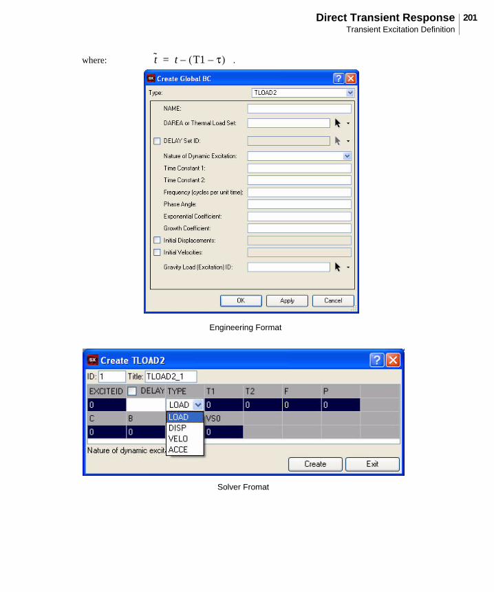
201Direct Transient ResponseTransient Excitation Definition
where: .t t T1 τ–( )–=
Engineering Format
Solver Fromat

Transient Excitation Definition202
Field Contents
EXITED Identification number of DAREA entry that defines . You can double click in this field to select an existing DAREA or create a new one.
DELAY Defines time delay . You can double click in this field to create or select an existing DELAY entry that defines . or you can directly enter the value of that will be used for all degrees-of-freedom that are excited by this dynamic load entry.
TYPE Defines the type of the dynamic excitation as defined in Table 5-3.
T1, T2 Time constants
F Frequency (cycles per unit time).
P Phase angle (degrees).
C Exponential coefficient
B Growth coefficient
US0 Factor for initial displacements.
VS0 Factor for initial velocities.
A
ττ τ

203Direct Transient ResponseTransient Excitation Definition
Time Delay -- DELAY Entry
The DELAY entry defines the time delay in an applied load.
The node to which it is applied is selected separately. Any number of DELAY entries may be used; as long as they are grouped in the same Nastran Set.
Field Contents
Card Type of MD Nastran bulk data entry that will be created.
Di Component number. Cell value is , the Time delay for that component
τ
Engineering Format
Solver Fromat
τi

Transient Excitation Definition204
Dynamic Load Tabular Function – TABLEDi EntriesThe TABLEDi entries (i = 1 through 4) each define a tabular function for use in generating frequency-dependent dynamic loads. The form of each TABLEDi entry varies slightly, depending on the value of i, as does the algorithm for y(x). The x values need not be evenly spaced.
The TABLED1, TABLED2, and TABLED3 entries linearly interpolate between the end points and linearly extrapolate outside of the endpoints as shown in Figure 5-2. TABLED1 has the added option to perform logarithmic interpolation between points, also. The TABLED4 entry uses the endpoint values for values beyond the endpoints.
Figure 5-2 Interpolation and Extrapolation for TABLED1, TABLED2,and TABLED3 Entries
y
x
Linear Extrapolation of Segment x2 – x1
Linear Extrapolation of Segment x6 – x7
Linear Interpolation Between Endpoints
x1 x2 x3 x4 x5 x6 x7

205Direct Transient ResponseTransient Excitation Definition
.The TABLED1 entry has the appears as follows:
To enter X-Y pairs, click Add once for each set of X-Y pairs. Click in the box for the first X value and type in the value. Use the tab key to advance to each successive field. When all values are entered, the table is defined and you can click Create. To see a plot of your x-y pairs, click Update then select Fit Curves from the View menu.
Field Contents
TID Table identification number.
XAXIS Specifies a linear or logarithmic interpolation for the x-axis.
YAXIS Specifies a linear or logarithmic interpolation for the y-axis.
xi, yi Tabular values. Values of x are frequency in cycles per unit time.

Transient Excitation Definition206
The TABLED1 entry uses the algorithm
(5-16)
The algorithms used for interpolation and extrapolation are as follows:
X-Y pairs are entered in the same manner for all tables. For the remaining tables we will look only the fields that are unique to that table type. The TABLED2 entry appears as follows:
The TABLED2 entry uses the algorithm
(5-17)
The TABLED3 entry has the following format:
XAXIS YAXIS yT(x)
LINEAR LINEAR
LOG LINEAR
LINEAR LOG
LOG LOG
Field Contents
TID Table identification number.
X1 Table parameter.
Field Contents
TID Table identification number.
X1, X2 Table parameters.
y yT x( )=
xj x–xj xi–---------------yi
x xi–xj xi–---------------yj+
xj x⁄( )lnxj xi⁄( )ln
-----------------------yix xi⁄( )lnxj xi⁄( )ln
-----------------------yj+
xj x–xj xi–--------------- yiln
x xi–xj xi–--------------- yjln+exp
xj x⁄( )lnxj xi⁄( )ln
----------------------- yilnx xi⁄( )lnxj xi⁄( )ln
----------------------- yjln+exp
y yT x X1–( )=

207Direct Transient ResponseTransient Excitation Definition
The TABLED3 entry uses the algorithm
(5-18)
The TABLED4 entry has the following format:
The TABLED4 entry uses the algorithm
(5-19)
is the degree of the power series. When , is used for ; when , is used for . This condition has the effect of placing bounds on the table; there is no extrapolation outside of the table boundaries.
Dynamic Load Set Combination -- DLOADOne of the requirements of transient loads is that all TLOAD1s and TLOAD2s must have unique SIDs. If they are to be applied in the same analysis, they must be combined using the DLOAD Bulk Data entry. The total applied load is constructed from a combination of component load sets as follows:
(5-20)
where:
Field Contents
TID Table identification number.
Xi Table parameters. .
overall scale factor
scale factor for i-th load set
i-th set of loads
total applied load
y yTx X1–
X2--------------- =
X2 0.0; X3 X4<≠( )
y Aix X1–
X2--------------- i
i 0=
N
=
N x X3< X3 x x X4> X4 x
P{ } S Si Pi{ }i=
S =
Si =
Pi=
P=

Transient Excitation Definition208
The DLOAD entry is created automatically by SimXpert.
Transient Excitation ConsiderationsA number of important considerations must be remembered when applying transient loads. It is important to avoid defining discontinuous forcing functions when describing applied loads. The numerical integration of discontinuous forcing functions may cause different results for the same analysis run on different computers because of slight numerical differences on different computer types. If the analysis calls for loadings with sharp impulses, it is best to smooth the impulse over at least one integration time increment.
The loading function must accurately describe the spatial and temporal distribution of the dynamic load. Simplifying assumptions must not change the character of the load in magnitude or location.

209Direct Transient ResponseExample
Example
Transient Analysis of a Two-DOF ModelConsider the two-DOF system shown in Figure 5-3. Direct transient response is run with an initial
displacement of 0.1 meter at node 2. The analysis is run for a duration of 10 seconds with a of 0.01 second. Damping is neglected in the analysis.
Figure 5-3 Two-DOF Model
Enter the Structures Workspace and Set Metric Units:1. Startup SimXpert and select Structures as the default workspace from the startup panel.
2. From the Tools menu, select Options, then choose Units Manager from the tree.
3. Click Standard Units.
4. Scroll down to, then select the row with Standard Metric Units (m, kg, s,...).
5. Click OK.
6. Click OK.
Create a Part:1. From the Part toolbox, select Create.
2. Click OK.
Create Nodes1. On the Nodes/Elements tab, select Node from the Create group.
2. Click in the Locations text box.
3. In the X,Y,Z Input box, enter 0 0 0, then click OK.
Δt
y
x
Node 1
Node 2
m1
m2
k1
k2

Example210
4. Repeat Step 3 for 0 1 0, and 0 2 0.
5. Click OK on the Node form.
Create Constraints and Loads1. On the LBCs tab, select General under the Constraint group.
2. Pull down BC Sub-Type to PSPC.
3. Enter Out of Plane for Name.
4. Click in the Pick Entities textbox.
5. Pull down the selection submenu on the Pick Filters toolbar and click Select All
6. Uncheck the checkbox for Ty.
7. Select Permanent Motion for the Constraint Type.
8. Click OK.
Turn on Node Numbering:1. From the Tools menu, click Identify
2. Select Nodes from the Pick Panel
3. Click All.
4. Notice that Node 1 is located at Y=0, Node 2 at Y=1, and Node 3 at Y=2.
Modeling Window Shows: Three unreferenced nodes are created in the y-direction.
Modeling Window Shows: PSPC[13456] is assigned to all three nodes.
Modeling Window Shows: Nodes labeled with their corresponding ID numbers.

211Direct Transient ResponseExample
Create Two Concentrated Masses1. On the Nodes/Elements tab, select Create/Create Element from the Element group.
2. Select 0D as the Element Type and CONM2 as the Element Sub-Type.
3. Click the Locations textbox.
4. Screen Pick Node 1 (the node with the lowest Y value)
5. Enter 0.1 for Mass Value.
6. Click Apply.
7. Change the Mass to 10.
8. Click the Locations textbox.
9. Select Node 2 (the middle node)
10. Click Apply.
Create Two Spring Elements1. Select 1D as the Element Type and CELAS2 as the Element Sub-Type.
2. Enter the values:
3. Click the Location textbox.
4. Pick Node 1 and Node 2.
5. Click Apply.
6. Enter the values:
Modeling Window Shows: Node 1 has an associated concentrated mass.
Modeling Window Shows: Node 2 has an associated concentrated mass.
Elastic Property Value (K)
100
Component Number (C1) 2
Component Number (C2) 2
Elastic Property Value (K)
1.0e4
Component Number (C1) 2
Component Number (C2) 2

Example212
7. Click the Location textbox.
8. Pick Node 2 and Node 3.
9. Click OK.
Create Constraints and Loads
Constrain the Base of the Model:10. On the LBCs tab, select General under the Constraint group.
11. Enter Base for Name.
12. Click in the Pick Entities textbox.
13. Select Node 3 (the node with the greatest y value)
14. Uncheck all checkboxes except for (Dof 2) Enforced Diplacement Y.
15. Click OK.
Create the Initial Conditions:1. On the LBCs tab, select Initial Transient Condition under the Global group.
2. Enter Initial Displacement for Name.
3. Click in the Pick entities text box and select Node 2 (the middle node)
4. Pull down Component Number to 2
5. Enter 0.1 for Initial Displacement.
6. Click OK.
Setup Analysis1. Right-click FileSet and select Create New Nastran Job
2. Enter Two_DOF as the Job Name
3. On the Solution Type drop down menu, select Direct Transiet Analysis(SOL 109).
4. Click the ellipses (...) on Solver Input file.
5. Choose the file path and enter Two_DOF for the File name.
6. Click Save.
7. Click OK.
Add Time Step:1. Double-click Loadcase Control.
2. Select Time Step Definition Table.
Modeling Window Shows: SPC[2] is assigned to the node with the greatest y dimension.

213Direct Transient ResponseExample
3. Right-click the window, choose Add.
4. Enter 1000 for the Number of Time Steps.
5. Enter 0.01 in the Time Increment box.
6. For the Skip Factor enter 1.
7. Click Apply.
8. Click OK.
Run the Analysis:1. Right click the job, Two_DOF, and select Run.
Create Charts of Result data
Attach Results:
An .xdb file will be created when the analysis has been successfully completed.
1. From the File menu and select Attach Results.
2. Click the browse button
3. Select the file two_dof.xdb.
4. Click Open.
5. Select Result as the Attach Option.
6. Click OK.
Create Graphs of Displacement versus Time:1. On the Result tab, select Chart.
2. Click on the subcase to select all time steps.
3. Select Displacement, Translational under Result Type.
4. Select Y Component under Derivation.
5. Click in Target Entities list box and pick Node 1 from the window.

Example214
6. Click Add Curves.

215Direct Transient ResponseExample
7. When finished with Node 1, click Clear Plot. Clear Node 1 from the Target Entities list box. Then repeat the steps for plotting for Node 2,
Notice the two different frequencies apparent in this graph. This is called beating.

Example216

217Modal Transient Response
Modal Transient Response

Modal Versus Direct Transient Response218
Modal Versus Direct Transient ResponseSome general guidelines can be used in selecting modal transient response analysis versus direct transient response analysis. These guidelines are summarized in Table 6-1.
In general, larger models may be solved more efficiently in modal transient response because the numerical solution is a solution of a smaller system of uncoupled equations. This result is certainly true if the natural frequencies and mode shape were computed during a previous stage of the analysis. Using Duhamel’s integral to solve the uncoupled equations is very efficient even for very long duration transients. On the other hand, the major portion of the effort in a modal transient response analysis is the calculation of the modes. For large systems with a large number of modes, this operation can be as costly as direct integration. This is especially true for high frequency excitation. To capture high frequency response in a modal solution, less accurate high frequency modes must be computed. For small models with a few time steps, the direct method may be the most efficient because it solves the equations without first computing the modes. The direct method is more accurate than the modal method because the direct method is not concerned with mode truncation. For systems with initial conditions, direct transient response is the only choice.
Table 6-1 provides a starting place for evaluating which method to use. Many additional factors may be involved in the choice of a method, such as contractual obligations or local standards of practice.
Table 6-1 Modal Versus Direct Transient Response
Modal Direct
Small Model X
Large Model X
Few Time Steps X
Many Time Steps X
High Frequency Excitation X
Normal Damping X
Higher Accuracy X
Initial Conditions X

219Modal Transient ResponseOverview and Definition
Overview and DefinitionModal transient response is an alternative approach to computing the transient response of a structure. This method uses the mode shapes of the structure to reduce the size, uncouple the equations of motion (when modal or no damping is used), and make the numerical integration more efficient. Since the mode shapes are typically computed as part of the characterization of the structure, modal transient response is a natural extension of a normal modes analysis.
As a first step in the formulation, transform the variables from physical coordinates to modal
coordinates by
(6-1)
The mode vectors are used to transform the problem in terms of the behavior of the modes as opposed to the behavior of the nodes. Equation (6-1) represents an equality if all modes are used; however, because all modes are rarely used, the equation usually represents an approximation.
To proceed, temporarily ignore the damping, resulting in the equation of motion
(6-2)
If the physical coordinates in terms of the modal coordinates (Equation (6-1) is substituted into Equation (6-2)), the following equation is obtained:
(6-3)
This is now the equation of motion in terms of the modal coordinates. At this point, however, the equations remain coupled.
To uncouple the equations, premultiply by to obtain
(6-4)
where:
The final step uses the orthogonality property of the mode shapes to formulate the equation of motion in terms of the generalized mass and stiffness matrices that are diagonal matrices. These matrices do not have off diagonal terms that couple the equations of motion. Therefore, in this form, the modal equations
modal (generalized) mass matrix
modal (generalized) stiffness matrix
modal force vector
u{ }ξ{ }
u t( ){ } φ[ ] ξ t( ){ }=
φ[ ]
M[ ] u·· t( ){ } K[ ] u t( ){ }+ P t( ){ }=
M[ ] φ[ ] ξ·· t( ){ } K[ ] φ{ } ξ t( ){ }+ P t( ){ }=
φ[ ]T
φ[ ]TM[ ] φ[ ] ξ··{ } φ[ ]T
K[ ] φ[ ] ξ{ }+ φ[ ]TP t( ){ }=
φ[ ]TM[ ] φ[ ]
φ[ ]TK[ ] φ[ ]
φ[ ]TP{ }

Overview and Definition220
of motion are uncoupled. In this uncoupled form, the equations of motion are written as a set of uncoupled SDOF systems as
(6-5)
where:
Note that there is no damping in the resulting equation. The next subsection describes how to include damping in modal transient response.
Once the individual modal responses are computed, physical responses are recovered as the
summation of the modal responses
(6-6)
Since numerical integration is applied to the relatively small number of uncoupled equations, there is not
as large a computational penalty for changing as there is in direct transient response analysis.
However, a constant is still recommended.
Another efficiency option in the modal transient solution is that the output time interval may be greater than the solution time interval. In many cases, it is not necessary to sample output response at each solution time. For example, if the solution is performed every 0.001 second, the results can be output every fifth time step or every 0.005 second. This efficiency reduces the amount of output.
Units in Dynamic AnalysisBecause there is more input in dynamic analysis than in static analysis, it is easier to make a mistake in units when performing a dynamic analysis. The most frequent source of error in dynamic analysis is incorrect specification of the units, especially for mass and damping.
i-th modal mass
i-th modal stiffness
i-th modal force
miξ··
i t( ) kiξi t( )+ pi t( )=
mi
ki
pi
ξi t( )
u t( ){ } φ[ ] ξ t( ){ }=
Δt
Δt

221Modal Transient ResponseOverview and Definition
Table 6-2 shows typical dynamic analysis variables, fundamental and derived units, and common English and metric units. Note that for English units all “lb.” designations are . The use of “lb.” for mass (i.e.,
) is avoided.
Table 6-2 Engineering Units for Common Variables
Variable Dimensions*Common
English UnitsCommon
Metric Units
Length L in m
Mass M kg
Time T sec sec
Area
Volume
Velocity in / sec m / sec
Acceleration
Rotation -- rad rad
Rotational Velocity rad / sec rad / sec
Rotational Acceleration
Circular Frequency rad / sec rad / sec
Frequency cps; Hz cps; Hz
Eigenvalue
Phase Angle -- deg deg
Force lb N
Weight lb N
Moment in-lb N-m
Mass Density
Young’s Modulus
Poisson’s Ratio -- -- --
Shear Modulus
Area Moment of Inertia
Torsional Constant
Mass Moment of Inertia
Stiffness N / m
Viscous Damping Coefficient
lb-sec / in N-sec / m
lbf
lbm
lb-sec2
in⁄
L2
in2
m2
L3
in3
m3
LT1–
LT2–
in sec2⁄ m sec
2⁄
T1–
T2–
rad sec2⁄ rad sec
2⁄T
1–
T1–
T2–
rad2
sec2⁄ rad
2sec
2⁄
MLT2–
MLT2–
ML2T
2–
ML3–
lb-sec3
in4⁄ kg m
3⁄ML
1–T
2–lb in
2⁄ Pa; N m2⁄
ML1–T
2–lb in
2⁄ Pa; N m2⁄
L4
in4
m4
L4
in4
m4
ML2
in-lb-sec2
kg-m2
MT2–
lb in⁄MT
1–

Overview and Definition222
Damping
If the damping matrix exists, the orthogonality property (see Equation (4-13) in the Normal Modes document) of the modes does not, in general, diagonalize the generalized damping matrix
(6-7)
In the presence of a matrix, the modal transient approach solves the coupled problem in terms of modal coordinates using the direct transient numerical integration approach described as follows:
(6-8)
where (6-9)
These equations are similar to the direct transient method except that they are in terms of modal coordinates. Since the number of modes used in a solution is typically much fewer than the number of physical variables, the direct integration of the modal equations is not as costly as with physical variables.
Stress
Strain -- -- --
*
where: Denotes length M Denotes massT Denotes time -- Denotes dimensionless
Table 6-2 Engineering Units for Common Variables (continued)
Variable Dimensions*Common
English UnitsCommon
Metric Units
ML1–T
2–lb in
2⁄ Pa; N m2⁄
B[ ]
φ[ ]TB[ ] φ[ ] diagonal≠
B[ ]
A1[ ] ξn 1+{ } A2{ } A3[ ] ξn{ } A4[ ] ξn 1–{ }+ +=
A1[ ] φT M
Δt2
-------- B2Δt--------- K
3----+ + φ=
A2{ } 13--- φ
TPn 1+ Pn Pn 1–+ +{ }=
A3[ ] φT 2M
Δt2
-------- K3----– φ=
A4[ ] φT M
Δt2
--------–B
2Δt--------- K
3----–+ φ=

223Modal Transient ResponseOverview and Definition
If damping is applied to each mode separately, the decoupled equations of motion can be maintained.
When modal damping is used, each mode has damping . The equations of motion remain uncoupled
and have the following form for each mode:
(6-10)
or
(6-11)
where:
The TABDMP1 table defines the modal damping ratios. A table is created by the frequency-damping pairs specified in the TABDMP1 entry. The solution refers to this table for the damping value to be
bi
miξ··
i t( ) biξ·
i t( ) kiξi t( )+ + pi t( )=
ξ·· i t( ) 2ζiωiξ·
i t( ) ωi2ξi t( )+ +
1mi-----pi t( )=
ζi bi 2miωi( )⁄= modal damping ratio≡
ωi2
ki mi modal frequency (eigenvalue)≡⁄=

Overview and Definition224
applied at a particular frequency. A particular TABDMP1 table is activated by selecting it when setting up your analysis.
If TYPE is “G” the damping values are in units of equivalent viscous dampers, as follows:
Field Contents
TYPE Type of damping units:G (default)CRITQ
X Value Frequency value (cycles per unit time).
Y Value Damping value in the units specified for the model.
bigiωi-----Ki=

225Modal Transient ResponseOverview and Definition
If TYPE is “CRIT”, the damping values are in the units of fraction of critical damping . If TYPE
is “Q”, the damping values are in the units of the amplification or quality factor, Q. These constants are related by the following equations:
At resonance, the three types of damping are related by the following equations:
(6-12)
The values of (units = cycles per unit time) and define pairs of frequencies and dampings. Note
that can be entered as structural damping (default), critical damping, or quality factor. The entered damping is internally converted to structural damping using Equation (6-12). Straight line interpolation
C C0⁄
C C0⁄ g 2⁄=
Q1 2C C0⁄( )⁄
1 g⁄
=
ζi
bi
bcr-------
Gi
2-----= =
bcr 2miωi=
Qi1
2ζi------- 1
Gi-----= =
fi gi
gi

Overview and Definition226
is used for modal frequencies between consecutive values. Linear extrapolation is used at and beyond the ends of the table. We will demonstrate this with an example table.
Figure 6-1 Example TABDMP1 Input
This table is created by selecting TABDMP1 from the Tables submenu of the Materals and Properties tab.
Since we have 4 x-y pairs of data, click Add (+) 4 times. Click in the box for the first X value and type in the values using the Enter key to advance to each successive field. When all values are entered, the table is defined and you can click OK.
In our example, if modal damping is entered as shown in Figure 6-1and if modes exist at 1.0, 2.5, 3.6, and 5.5 Hz, SimXpert interpolates and extrapolates as shown in Figure 6-2 and Table 6-3. Note that there
fi

227Modal Transient ResponseOverview and Definition
is no table entry at 1.0 Hz; SimXpert uses the first two table entries at and to
extrapolate the value for .
Figure 6-2 Example TABDMP1
Table 6-3 Example TABDMP1 Interpolation/Extrapolation
With the modal equations in the form of Equation (6-11), an efficient uncoupled analytical integration algorithm is used to solve for modal response as decoupled SDOF systems. Each of the modal responses is computed using
(6-13)
Entered Computed
X Y f g
2.0 0.16 1.0 0.14
3.0 0.18 2.5 0.17
4.0 0.13 3.6 0.15
6.0 0.13 5.5 0.13
f 2.0= f 3.0=
f 1.0=
0.10
0.20
2.0 4.0 6.0
f(Hz)
0.0
= entered value
= computed value
++
+ +
+
0, No initial conditions for modal transient response.
ξ t( ) ebt– 2m⁄ ξo ωdtcos
ξ· o b 2m( )⁄ ξo+
ωd------------------------------------- ωdtsin+
ebt– 2m⁄ 1
mωd----------- e
bτ 2m⁄p τ( ) ωd t τ–( )dτsin
0
t
+
=

Overview and Definition228
In a modal transient analysis, you may add nonmodal damping (CVISC, CDAMPi, GE on the MATi
entry, or PARAM,G). With nonmodal damping, there is a computational penalty due to the coupled matrix, causing the coupled solution algorithm to be used. In modal transient response analysis, it is recommended that you use only modal damping (TABDMP1). If discrete damping is desired, direct transient response analysis is recommended.
Note that there are no nonzero initial conditions for modal transient response analysis.
Mode Truncation It is possible that not all of the computed modes are required in the transient response solution. Often, only the lowest few suffice for dynamic response calculation. It is quite common to evaluate the frequency content of transient loads and determine a frequency above which no modes are noticeably excited. This frequency is called the cutoff frequency. The act of specifically not using all of the modes of a system in the solution is termed mode truncation. Mode truncation assumes that an accurate solution can be obtained using a reduced set of modes. The number of modes used in a solution is controlled in a modal transient response analysis through a number of methods.
B[ ]

229Modal Transient ResponseOverview and Definition
The frequency range selected on the Eigenvalue Extraction form is one means to control the frequency range used in the transient response solution. This range is entered when you set up your job for analysis. The Eigenvalue extraction form appears as follows:
Also, three parameters are available to limit the number of modes included in the solution and can be used as an alternative to the above. PARAM,LFREQ gives the lower limit on the frequency range of retained modes, and PARAM,HFREQ gives the upper limit on the frequency range of retained modes.
Start of Frequency Range of Interest
End of Frequency Range of Interest

Overview and Definition230
PARAM,LMODES gives the number of the lowest modes to be retained. These parameters are accessed by selecting PARAM from the LBCs tab.
These parameters can be used to include the desired set of modes. Note that the default is for all computed modes to be retained.
It is very important to remember that truncating modes in a particular frequency range may truncate a significant portion of the behavior in that frequency range. Typically, high frequency modes are truncated because they are more costly to compute. So, truncating high frequency modes truncates high frequency response. In most cases, high frequency mode truncation is not of concern. You should evaluate the truncation in terms of the loading frequency and the important characteristic frequencies of the structure.
Dynamic Data RecoveryIn modal transient response analysis, two options are available for recovering displacements and stresses: mode displacement method and matrix method. Both methods give the same answers, although with cost differences.

231Modal Transient ResponseOverview and Definition
The mode displacement method computes the total physical displacements for each time step from the modal displacements and then computes element stresses from the total physical displacements. The number of operations is proportional to the number of time steps.
The matrix method computes displacements per mode and element stresses per mode, and then computes physical displacements and element stresses as the summation of modal displacements and element stresses. Costly operations are proportional to the number of modes.
Since the number of modes is usually much less that the number of time steps, the matrix method is usually more efficient and is the default. The mode displacement method can be selected by using PARAM,DDRMM,-1.
The mode acceleration method is another form of data recovery for modal transient response analysis. This method can provide better accuracy since detailed local stresses and forces are subject to mode truncation and may not be as accurate as the results computed with the direct method.

Transient Excitation Definition232
Transient Excitation DefinitionAn important aspect of a transient response analysis is the definition of the loading function. In a transient response analysis, the force must be defined as a function of time. The following entries are used for the transient load definition:
The particular entry chosen for defining the dynamic loading is largely a function of user convenience for concentrated loads. Pressure and distributed loads, however, require a more complicated format.
There are two important aspects of dynamic load definition. First, the location of the loading on the structure must be defined. Since this characteristic locates the loading in space, it is called the spatial distribution of the dynamic loading. Secondly, the time variation in the loading is the characteristic that differentiates a dynamic load from a static load. This time variation is called the temporal distribution of the load. A complete dynamic loading is a product of spatial and temporal distributions.
Using Tables and Sets in SimXpert makes it possible to apply many complicated and temporally similar loadings with a minimum of input. Combining simple loadings to create complicated loading distributions that vary in position as well as time is also a straightforward task.
The remainder of this section describes the entries for transient excitation. The description is given in terms of the coefficients that define the dynamic load.
Time Dependent Loads -- TLOAD1 EntryThe TLOAD1 entry is the most general form in which to define a time dependent load. It defines a dynamic loading of the form
(6-14)
Entry Description Where to Input
TLOAD1 Defines a time-dependent dynamic load or enforced motion
TLOAD2
LSEQ Generates the spatial distribution of dynamic loads from static load entries
DLOAD Defines a dynamic loading condition as a linear combination of TLOADi sets.
Generated automatically by SimXpert
DAREA Defines scale factors for the spatial distribution of dynamic load BC / Create BC/ SPC BCDELAY Defines the time delay term in the equations of the dynamic
loading function
TABLEDi Tabular values versus time for generating dynamic loads
τ
P t( ){ } A F t τ–( )⋅{ }=

233Modal Transient ResponseTransient Excitation Definition
The coefficients of the force are defined in tabular format. You need not explicitly define a force at every instant in time for which the transient solution is evaluated. Only those values which describe the character of the loading are required. SimXpert interpolates linearly for intermediate values.
Field Contents
EXCITEID Identification number of DAREA or SPCD entry that defines . You can double click in this field to select an existing DAREA or create a new one.
DELAY Defines time delay . You can double click in this field to create or select an existing DELAY entry that defines .
TYPE Defines the type of the dynamic excitation as defined in Table 6-4.
Engineering Format
Solver Fromat
A
ττ

Transient Excitation Definition234
Time Dependent Loads – TLOAD2 EntryThe TLOAD2 entry is a general analytical form with which to define a time-dependent load. The value of the force at a particular instant in time is determined by evaluating the analytic function at the specific time. You enter the appropriate constants in the function.
The TLOAD2 entry defines dynamic excitation in the form:
(6-15)
TID Identification number of TABLEDi entry that gives . You can double click in this field to select an existing TABLEDi or create a new one.
US0 Factor for initial displacements of the enforced degrees-of-freedom.
VS0 Factor for initial velocities of the enforced degrees-of-freedom.
Table 6-4 Excitation Function Types
TYPE Type of Dynamic Excitation
LOAD Applied Load (Force or Moment)
DISP Enforced Displacement using large mass or SPC/SPCD dataVELO Enforced Velocity using large mass or SPC/SPCD dataACCE Enforced Acceleration using large mass or SPC/SPCD data
Field Contents
F t( )
P t( ){ }0 , t T1 τ+( ) or t T2 τ+( )><
AtB
eCt
2πF t P+( )cos , T1 τ+( ) t T2 τ+( )≤ ≤
=

235Modal Transient ResponseTransient Excitation Definition
where: .t t T1 τ–( )–=
Engineering Format
Solver Fromat

Transient Excitation Definition236
Field Contents
EXCITEID Identification number of DAREA or SPCD entry that defines . You can double click in this field to select an existing DAREA or create a new one.
DELAY Defines time delay . You can double click in this field to create or select an existing DELAY entry that defines .
TYPE Defines the type of the dynamic excitation as defined in Table 6-4.
T1, T2 Time constants
F Frequency (cycles per unit time).
P Phase angle (degrees).
C Exponential coefficient
B Growth coefficient
US0 Factor for initial displacements of the enforced degrees-of-freedom.
VS0 Factor for initial velocities of the enforced degrees-of-freedom.
A
ττ

237Modal Transient ResponseTransient Excitation Definition
Spatial Distribution of Loading – DAREA EntryThe DAREA entry defines the degrees of freedom where the dynamic load is to be applied and a scale factor to be applied to the loading. The DAREA entry provides the basic spatial distribution of the dynamic loading.
Field Contents
Card Type of MD Nastran bulk data entry that will be created.
Di Scale (area) factors for component i of dynamic loads.
MD Nastran Format
Engineering Format

Transient Excitation Definition238
A DAREA entry is selected by the TLOAD1 or TLOAD2 entry. Any number of DAREA entries may be used; as long as they are grouped in the same Nastran Set.
After entering data, you will click Store, then pick the node(s) to which the dynamic load is applied.
Time Delay -- DELAY Entry
The DELAY entry defines the time delay in an applied load.
Field Contents
Card Type of MD Nastran bulk data entry that will be created.
Di Time delay for component i of dynamic loads
τ
Engineering Format
Solver Fromat

239Modal Transient ResponseTransient Excitation Definition
After entering data, you will click Store, then pick the node(s) to which the delay in the dynamic load is to be applied.
Any number of DELAY entries may be used; as long as they are grouped in the same Nastran Set.
Dynamic Load Tabular Function – TABLEDi EntriesThe TABLEDi entries (i = 1 through 4) each define a tabular function for use in generating frequency dependent dynamic loads. The form of each TABLEDi entry varies slightly, depending on the value of i, as does the algorithm for y(x). The x values need not be evenly spaced.
The TABLED1, TABLED2, and TABLED3 entries linearly interpolate between the end points and linearly extrapolate outside of the endpoints as shown in Figure 6-3. TABLED1 has the added option to perform logarithmic interpolation between points, also. The TABLED4 entry uses the endpoint values for values beyond the endpoints.
Figure 6-3 Interpolation and Extrapolation for TABLED1, TABLED2,and TABLED3 Entries
y
x
Linear Extrapolation of Segment x2 – x1
Linear Extrapolation of Segment x6 – x7
Linear Interpolation Between Endpoints
x1 x2 x3 x4 x5 x6 x7

Transient Excitation Definition240
The TABLED1 entry has the appears as follows:
The TABLED1 entry uses the algorithm
(6-16)
Field Contents
X Interpolation Type
Specifies a linear or logarithmic interpolation for the x-axis.
Y Interpolation Type
Specifies a linear or logarithmic interpolation for the y-axis.
X Value, Y Value Tabular values. Values of x are frequency in cycles per unit time. Data is input in the same manner as described for TABDMP1 on page 225.
y yT x( )=

241Modal Transient ResponseTransient Excitation Definition
The algorithms used for interpolation and extrapolation are as follows:
X-Y pairs are entered in the same manner for all tables. For the remaining tables we will look only the fields that are unique to that table type. The TABLED2 entry appears as follows:
The TABLED2 entry uses the algorithm
XAXIS YAXIS yT(x)
LINEAR LINEAR
LOG LINEAR
LINEAR LOG
LOG LOG
Field Contents
TID Table identification number.
X1 Table parameter.
xj x–xj xi–---------------yi
x xi–xj xi–---------------yj+
xj x⁄( )lnxj xi⁄( )ln
-----------------------yix xi⁄( )lnxj xi⁄( )ln
-----------------------yj+
xj x–xj xi–--------------- yiln
x xi–xj xi–--------------- yjln+exp
xj x⁄( )lnxj xi⁄( )ln
----------------------- yilnx xi⁄( )lnxj xi⁄( )ln
----------------------- yjln+exp

Transient Excitation Definition242
(6-17)
The TABLED3 entry has the following format:
The TABLED3 entry uses the algorithm
(6-18)
Field Contents
TID Table identification number.
X1, X2 Table parameters.
y yT x X1–( )=
y yTx X1–
X2--------------- =

243Modal Transient ResponseTransient Excitation Definition
The TABLED4 entry has the following format:
The TABLED4 entry uses the algorithm
(6-19)
is the degree of the power series. When , is used for ; when , is used for . This condition has the effect of placing bounds on the table; there is no extrapolation outside of the table boundaries.
TABLED1/ TLOAD1 Example
First describe the time variation of the load. Remember that the solver will extrapolate linearly for points beyond this table.
Field Contents
TID Table identification number.
Xi Table parameters. .X2 0.0; X3 X4<≠( )
y Aix X1–
X2--------------- i
i 0=
N
=
N x X3< X3 x x X4> X4 x

Transient Excitation Definition244
1. On the Materials and Properties tab, select Table/NastranBDF/TABLED1 from the Element Properties group.
2. Click ADD (+) four times.
3. Click in the box for the first X value and type in the following data, using the tab key to advance between fields
4. Click OK.
Define the delay
1. On the LBCs tab, select Force from the Loads group.
X Y
0 0.0
3000 0.0
0.3 1
2 1

245Modal Transient ResponseTransient Excitation Definition
2. Enter the following data:
3. Check D1 then enter 0.2 and click Store then Exit
4. Screen pick the Node for load application.
5. Click Done then Exit in the Pick Panel.
Create the static loading
1. Right click on LBC in the Model Browser and select New BC > Nodal BC > FORCE.
2. Click Store, then Exit.
3. Screen pick a node.
4. Click Done then Exit in the pick panel.
Create the dynamic loading
1. Right click on Global BC in the Model Browser and New Global BC > RLOAD1.
2. Double click in EXCITE ID and select the Force from the Model Browser.
3. Double click in DELAY and select the Delay from the Model Browser.
F 4
Direction X 1
Direction Y 0
Direction Z 0

Transient Excitation Definition246
4. Double click in TID and select TABLED1 from the pop-up window
On the TLOAD1 entry is a reference to the applied force (with Set ID 4), the DELAY before the application of the load (Set ID 3), and the description of the time dependency, TABLED1 (Set ID 1). The FORCE entry with Set ID 4 positions the loading on the selected node in the 1 direction with a scale factor of 4.0 applied to the load. The DELAY entry with Set ID 3 delays the loading on the selected node in the 1 direction by 0.2 units of time. The TABLED1 entry with Set ID 1defines the load time history in tabular form. The result of these entries is a dynamic load applied to the selected node, component T1, scaled by 4.0 and delayed by 0.2 units of time.
The figure below shows the applied load (scaled by the FORCE entry and time shifted by the DELAY entry).

247Modal Transient ResponseTransient Excitation Definition
Integration Time StepThe TSTEP entry is used to select the integration time step. This entry also controls the duration of the solution and which time steps are to be output. The integration time step must be small enough to represent accurately the variation in the loading. The integration time step must also be small enough to represent the maximum frequency of interest. The maximum frequency of interest is often called the cutoff frequency. It is recommended to use at least ten solution time steps per period of response for the cutoff frequency. For a given integration time step, integration errors increase with increasing natural frequency because there is an upper limit to the frequency that can be represented by a given time step. Also, integration errors accumulate with total time.
In specifying the duration of the analysis, it is important to use an adequate length of time to properly capture long period (low frequency) response. In many cases, the peak dynamic response does not occur at the peak value of load nor necessarily during the duration of the loading function. A good rule is: always solve for at least one cycle of response for the lowest frequency mode after the peak excitation.

Transient Excitation Definition248
The integration time step is entered during analysis setup. Once an analysis subcase has been defined, you can define the properties for the time step table. The Time Step Definition form appears as follows:
where:
Notice that you can have multiple time step definitions in one analysis.
Transient Excitation ConsiderationsA number of important considerations must be remembered when applying transient loads. Very sharp spikes in a loading function induce a high frequency transient response. If the high frequency transient response is of primary importance in an analysis, a very small integration time step must be used.
It is also important to avoid defining discontinuous forcing functions when describing applied loads. The numerical integration of discontinuous forcing functions may cause different results for the same analysis run on different computers because of slight numerical differences on different computer types. If the analysis calls for loadings with sharp impulses, it is best to smooth the impulse over at least one integration time increment.
Field Contents
Number of Time Steps Number of time steps with the value of Time Increment.
Time Increment Integration time step.
Skip Factor Skip factor, n, for output. Every n-th step will be saved for output.

249Modal Transient ResponseTransient Excitation Definition
The loading function must accurately describe the spatial and temporal distribution of the dynamic load. Simplifying assumptions must not change the character of the load in magnitude, location, or frequency content.

Example250
Example
Modal Transient Analysis of a Cantilever Beam ModelConsider the cantilever beam shown in Figure 6-4. Modal transient response (SOL 112) is run with loads applied to nodes 6 and 11 as shown in Figure 6-5. The analysis is run for a duration of 2 seconds with a
of 0.001 second. Modal damping of 5% critical damping is used for all modes. Modes up to 3000 Hz are computed using the Lanczos method.
Figure 6-4 Cantilever Beam Model with Applied Loads
Figure 6-5 Applied Loads for the Beam Model
Δt
y
x
6
p6(t)
11
p11(t)
Time (sec.)
6
-6
End Node Force (N)
0.5
Time (sec.)
3
-3
Node 6 Force(N)
0.1 0.5

251Modal Transient ResponseExample
Open SimXpert
Enter the Structures Workspace and Set Metric Units:1. Startup SimXpert and select Structures as the default workspace from the startup panel.
2. From the Tools menu, select Options, then choose Units Manager from the tree.
3. Click Standard Units.
4. Scroll down then click the row with Metric Units (m, kg, s,...).
5. Click OK.
6. Choose Structures.BC under the Entity Options branch of the tree.
7. Check the Display All Dir Vector checkbox and enter 25 as Vector Size as percentage of window size.
8. Click OK.
Create an Isotropic Material:1. On the Material and Properties tab, select Isotropic from the Materials group.
2. On the Material, enter:
3. Click OK.
Create an Element Property1. On the Material and Properties tab, select Beam from the 1D Properties group.
2. Click in the Material textbox and select Aluminum from the Model Browser.
3. Enter the following information:
Name Aluminum
Young’s Modulus 7.1e10
Poisson’s Ratio 0.33
Density 2.65e4
Note: This is weight (not mass) density
Name Aluminum Bar
Area 6.158e-4
Inertia ZZ 3.0e-8
Inertia YY 3.0e-8
Torsional constant 6.0e-8
Non Structural Mass 2.414

Example252
4. Click OK.
Create a Part1. On the Geometry tab, select Create Part from the Part group.
2. For the Title enter Beam.
3. Click OK.
Generate Curve1. On the Geometry tab, select Curve from the Curve group.
2. Click in the Entities text box.
3. In the X Y Z Input box, enter 0 0 0 then click OK
4. Enter 3 0 0 then click OK again
5. Click OK on Polyline Spline form
6. From the View menu, click Display, then click Fill.
Mesh Curve1. On the Meshing tab, select Curve from the Automesh group.
2. Click in the Curve to Mesh text box.
3. Screen pick the curve.
4. On the Mesher form, enter 0.3 for Element Size.
5. For Orientation Vector, enter 0 1 0 for X, Y, and Z respectively.
6. Click in the Element Property text box and then click on Aluminum Bar from the Model Browser tree.
7. Click OK.
Create Constraints and Loads
Constrain motion in Z-direction1. On the LBCs tab, select General from the Constraint group.
2. Change the Name to Z Motion.
3. Uncheck the boxes corresponding to Tx, Ty and Rz.
4. Click in the Pick Entities text box.
Modeling Window Shows:One line.
Modeling Window Shows:Ten elements created along the curve.
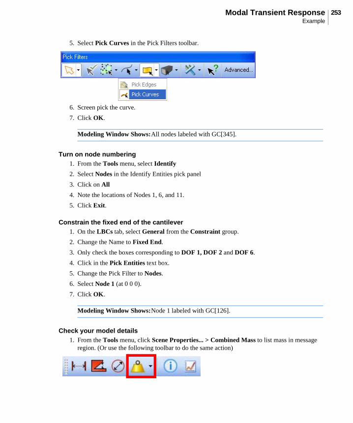
253Modal Transient ResponseExample
5. Select Pick Curves in the Pick Filters toolbar.
6. Screen pick the curve.
7. Click OK.
Turn on node numbering1. From the Tools menu, select Identify
2. Select Nodes in the Identify Entities pick panel
3. Click on All
4. Note the locations of Nodes 1, 6, and 11.
5. Click Exit.
Constrain the fixed end of the cantilever1. On the LBCs tab, select General from the Constraint group.
2. Change the Name to Fixed End.
3. Only check the boxes corresponding to DOF 1, DOF 2 and DOF 6.
4. Click in the Pick Entities text box.
5. Change the Pick Filter to Nodes.
6. Select Node 1 (at 0 0 0).
7. Click OK.
Check your model details1. From the Tools menu, click Scene Properties... > Combined Mass to list mass in message
region. (Or use the following toolbar to do the same action)
Modeling Window Shows:All nodes labeled with GC[345].
Modeling Window Shows:Node 1 labeled with GC[126].

Example254
Create the static loading1. On the LBCs tab, select Force from the Loads group.
2. For the Force Name, enter End Node Force, and enter:
3. Click in the Pick Entities text box.
4. Screen pick Node 11 (opposite end from Fixed End) then click Apply
5. For the new Force Name, enter Node 6 Force, and enter:
6. Click in Pick Entities text box.
7. Screen pick Node 6 (middle node)
8. Click OK.
Create the dynamic loading1. From the Tools menu, select Options, then choose GUI Options from the tree. Check box Solver
Card, and then click OK.
2. Double-click End Node Force in the Model Browser.
3. Check the box next Transient to activate the dynamic response cards.
4. Check Transient and pull down Type to TLOAD2.
Force Magnitude 6.
Direction - X 0
Direction - Y 1
Direction - Z 0
Modeling Window Shows:Force vector at node 11.
Force Magnitude 3.
Direction - X 0
Direction - Y 1
Direction - Z 0
Modeling Window Shows:Force vector at node 6

255Modal Transient ResponseExample
5. On the TLOAD2 form enter:
6. Click OK.
7. Double-click Node 6 Force in the Model Browser.
8. Check the box next Transient to activate the dynamic response cards.
9. Check Transient and pull down Type to TLOAD2.
10. On the TLOAD2 form enter
11. Click OK.
12. From the Tools menu, select Options, then Options Editor..., then choose GUI Options from the tree. Uncheck the box for Solver Card, and then click OK.
Setup Analysis1. Right-click FileSet and select Create New Nastran Job
2. Enter Cantilever as the Job Name.
3. Select Modal Transient Analysis (SOL 112).
4. Click the ellipses (...) on Sovler Input File.
5. Select the file path where the job will be exported and enter cantilever for the file name.
6. Click Save.
7. Click OK
Enter Conversion Factor from weight to mass units 1/G where G = 9.81 m/sec**21. Double-click Solver Control and select General Linear Solver Parameters.
2. Enter Weight - Mass conversion: 0.102
3. Click Apply.
T2 (Time Constant) 0.5
F (Frequency in cycles per unit time)
2
PHI (Phase angle in degrees)
90
DELAY 0.1
T2 0.5
F 4
PHI 90

Example256
4. Click Close.
Add Additional Output Request to the Subcase:1. Right Click Output Requests and select Add Subcase
2. Enter Dynamic Loading for the Name.
3. Select DefaultLbcSet
4. Set Modal Damping to Critical Damping (CRIT) and click OK
5. Right Click on Subcase: Dynamic Loading and select Add Output Requests
6. Right Click on Output Requests and select Add Displacement and click Apply
7. Right Click on Output Requests and select Add Acceleration and click Apply
8. Right Click on Output Requests and select Add Element Force and click Apply
9. Right Click on Output Requests and select Add Applied Load and click Apply
10. Click Close
Select Frequency Range for Modes:1. Double-click Loadcase Control and select Eigenvalue Extraction Parameters
2. Under Extraction, set Method to Lanczos.
3. Enter Lower = -0.1
4. Enter Upper = 3000
5. Set Number of Desired Roots to 0.
6. Click Apply.
Set Time Steps1. Select Time Step Definition Table.
2. Right click in the window and select Add (+).
3. Enter 2000 for the Number of Time Steps.
4. Enter 0.001 for the Time Increment.
5. Enter 1 for the Skip Factor.
6. Click Apply and then click Ok
Set Damping Parameters1. Right click on Damping Parameters and select Properties.
2. Right click in the window, select Add.
3. Enter 0 and 0.05 for Frequency and Damping respectively.
4. Click Apply.
5. Right click in the window, select Add.

257Modal Transient ResponseExample
6. Enter 1000 and 0.05 for Frequency and Damping respectively.
7. Click Apply.
8. Click OK.
Run the Analysis1. Right-click Cantilever and select Run.
Attach your Results1. Pull down the File menu and select Attach Results.
2. Click the browse button and navigate to where the job was run.
3. Select cantilever.xdb
4. Click Open
5. Select Results as the Attach Option.
6. Click OK.
Create Graph of applied loads on Nodes 6 and 111. From the Result toolbox, select Chart.
2. Click on the subcase in the Result Cases column to select all steps
3. Click on Applied Loads, Translational in the Result Type column
4. Click on Y Component in the Derivation column
5. For the Target Entities select Node 6 and Node 11
6. Click Add Curves.

Example258
7. The following chart will be displayed:
8. Notice the Time Delay of 0.1 seconds for Node 6
Create Graph of Displacement vs. Time1. Once again choose the subcase to select all steps
2. Click on Displacements, Translational in the Result Type column
3. Click on Y Component in the Derivation column
4. For the Target Entities select Nodes 6 and 11
5. Click Clear Plot
6. Click Add Curves

259Modal Transient ResponseExample
7. The following chart will be displayed:

Example260
8. Repeat the steps above for Acceleration, Translational
Plot the bending moment for the bars at node 61. Once again choose the subcase to select all steps
2. Click on Bar Forces, Rotational in the Result Type column
3. Click on Z Component in the Derivation column
4. For the Target Entities select Node 6
5. Click Clear Plot

261Modal Transient ResponseExample
6. Click Add Curves

Example262

261Direct Frequency Response
Direct Frequency Response

Modal Versus Direct Frequency Response262
Modal Versus Direct Frequency ResponseTwo different numerical methods can be used in frequency response analysis. The direct method solves the coupled equations of motion in terms of forcing frequency. The modal method utilizes the mode shapes of the structure to reduce and uncouple the equations of motion (when modal or no damping is used); the solution for a particular forcing frequency is obtained through the summation of the individual modal responses. The choice of the method depends on the problem.
Some general guidelines can be used in selecting modal frequency response analysis versus direct frequency response analysis. These guidelines are summarized in Table 7-1.
In general, larger models may be solved more efficiently in modal frequency response because the numerical solution is a solution of a smaller system of uncoupled equations. This result is certainly true if the natural frequencies and mode shape were computed during a previous stage of the analysis. Using the modal approach to solve the uncoupled equations is very efficient, even for very large numbers of excitation frequencies. On the other hand, the major portion of the effort in a modal frequency response analysis is the calculation of the modes. For large systems with a large number of modes, this operation can be as costly as a direct solution. This is especially true for high-frequency excitation. To capture high frequency response in a modal solution, less accurate high-frequency modes must be computed. For small models with a few excitation frequencies, the direct method may be the most efficient because it solves the equations without first computing the modes. The direct method is more accurate than the modal method because the direct method is not concerned with mode truncation.
Table 7-1 provides a starting place for evaluating which method to use. Many additional factors may be involved in the choice of a method, such as contractual obligations or local standards of practice.
Table 7-1 Modal Versus Direct Frequency Response
Modal Direct
Small Model X
Large Model X
Few Excitation Frequencies X
Many Excitation Frequencies X
High Frequency Excitation X
Nonmodal Damping X
Higher Accuracy X

263Direct Frequency ResponseOverview and Definition
Overview and DefinitionAn overview of the Direct Frequency Response Analysis is given here.
IntroductionFrequency Response Analysis is used to compute the steady state response of structures subjected to harmonic (oscillatory) excitations (forces). Examples of oscillatory excitation include rotating machinery, helicopter blades, and unbalanced tires. Oscillatory excitations are defined in the frequency domain, and can be in the form of forces and/or enforced motions (displacements, velocities, or accelerations).
Oscillatory loading is sinusoidal in nature. In its simplest case, this loading is defined as having a constant amplitude with a specific frequency. The steady-state oscillatory response is assumed to occur at the same frequency as the loading, but not necessarily in phase. Due to the presence of damping in the system, the response generally lags the excitation. Consequently, the peak response occurs a little while after the occurrence of the peak load.
Figure 7-1 Phase shift in steady state response
The results obtained from a frequency response analysis usually include the displacements, velocities, accelerations of nodes as well as stresses and forces of elements. The computed responses are complex numbers defined as magnitude and phase (with respect to the applied force), or as real and imaginary

Overview and Definition264
components which are vector components of the response in the real/imaginary plane. These quantities are graphically presented in Figure 7-2.
Figure 7-2 Complex Plane
where:
TheoryIn direct frequency response analysis, structural response is computed at discrete excitation frequencies by solving a set of coupled matrix equations using complex algebra. Begin with the damped forced vibration equation of motion with harmonic excitation. The dynamic equilibrium equation for harmonic excitation is:
= magnitude =
= phase angle =
= real component =
= imaginary component =
r (Real)
i (Imaginary)
uui
ur
θ
uur
2ui
2+
θ tan1–
ui ur⁄( )
ur u θcos
ui u θsin

265Direct Frequency ResponseOverview and Definition
(7-1)
where: [M], [B], and [K] are respectively the mass, damping and stiffness matrices of the structure, and {P} are amplitudes of the harmonic forces.
The assumption of the harmonic steady state response transforms the dynamic equilibrium equation of motion into a set of algebraic equations with complex coefficients. For this assumption of steady state response to be valid, the excitation forces at all locations must be at the same frequency, though not necessarily at the same phase. Furthermore the response is assumed to be linear.
Method of solutionIn direct frequency response analysis, the response is computed at discrete excitation frequencies by solving directly a set of coupled matrix equations with complex coefficients. For harmonic steady state response (the basis of a frequency response analysis), assume the displacement to be of the form:
where {u(ω)} is a complex displacement vector. Taking the first and second derivatives of the above equation, we obtain the following expressions for the velocity and acceleration vectors:
Substituting the above expressions for , , and into Equation (7-1), transforms into:
The above equation represents a system of simultaneous algebraic equations with complex coefficients. The left hand side of the equation is complex because of the damping, and the right hand side is complex because of the phase differences of the excitation forces at different nodes. The solution of this equation with complex arithmetic produces the displacement vector {u(ω)}, for the excitation {P(ω)}. You need to solve one set of such complex equations for each excitation frequency. In SimXpert structures, you can select a range of excitation frequencies for a single job, and the amplitude of the forces can be frequency dependent.
Damping
The damping matrix [B] comprises terms obtained from damping elements. The contributions of the overall structural damping coefficient (G), and the elemental structural damping coefficient (as defined in the material properties) are added to the stiffness matrix directly, making its coefficients complex:
M[ ] X·· t( ){ } B[ ] X· t( ){ } K[ ] X t( ){ }+ + P ω( ){ }eiωt=
X{ } u ω( ){ }eiωt=
X·{ } iω u ω( ){ }eiωt=
X··{ } ω2– u ω( ){ }eiωt=
X t( ) X· t( ) X·· t( )
ω2M– iωB K+ +[ ] u ω( ){ } P ω( ){ }=
K[ ] 1 iG ) K[ ] iΣGE KE[ ]+ +(=

Overview and Definition266
where: [K] = global stiffness matrix
G = overall structural damping coefficient (G)
[KE] = element stiffness matrix
GE = element structural damping coefficient (damping coefficient in material properties)
Consequently all types of damping can be used in the same direct frequency response analysis. Furthermore, it is not necessary to assume an equivalent viscous form for structural damping.
The overall structural damping value (G) is defined as solution parameter during analysis setup.

267Direct Frequency ResponseOverview and Definition
The elemental structural damping value (GE) is defined on the material properties form

Frequency-Dependent Excitation Definition268
Frequency-Dependent Excitation DefinitionAn important aspect of a transient response analysis is the definition of the loading function. In a frequency response analysis, the force must be defined as a function of frequency. To create a Frequency-Dependent dynamic repsonse, use the Dyanamic tab on the Loads and Pressure cards found on the LBCs tab. For example, the Force form:
The particular entry chosen for defining the dynamic loading is largely a function of user convenience for concentrated loads. Pressure and distributed loads, however, require a more complicated format.
There are two important aspects of dynamic load definition. First, the location of the loading on the structure must be defined. Since this characteristic locates the loading in space, it is called the spatial distribution of the dynamic loading. Secondly, the frequency variation in the loading is the characteristic that differentiates a dynamic load from a static load. This frequency variation is called the temporal distribution of the load. A complete dynamic loading is a product of spatial and temporal distributions.
Using Tables and load combinations in SimXpert makes it possible to apply many complicated and temporally similar loadings with a minimum of input. Combining simple loadings to create complicated loading distributions that vary in position as well as time is also a straightforward task.
The remainder of this section describes the entries for frequency-dependent excitation. The description is given in terms of the coefficients that define the dynamic load.

269Direct Frequency ResponseFrequency-Dependent Excitation Definition
Frequency-Dependent Loads – RLOAD1 EntryThe RLOAD1 entry is a general form in which to define a frequency-dependent load. It defines a dynamic loading of the form
(7-2)P f( ){ } A C f( ) iD f( )+[ ]ei θ 2πfτ–{ }{ }=

Frequency-Dependent Excitation Definition270
The values of the coefficients are defined in tabular format on a TABLEDi entry. You need not explicitly define a force at every excitation frequency. Only those values that describe the character of the loading are required. MD Nastran will interpolate for intermediate values.
Field Contents
EXCITEID Identification number of the DAREA entry set that defines A, the Thermal Load Set or a BC Set.
DELAY Identification number of the DELAY entry set that defines .
MD Nastran Format
Engineering Format
τ

271Direct Frequency ResponseFrequency-Dependent Excitation Definition
For each field you can double click in the databox and choose to Select or Create the entry.
Frequency-Dependent Loads – RLOAD2 EntryThe RLOAD2 entry is a variation of the RLOAD1 entry used for defining a frequency-dependent load. Whereas the RLOAD1 entry defines the real and imaginary parts of the complex load, the RLOAD2 entry defines the magnitude and phase.
The RLOAD2 entry defines dynamic excitation in the form
(7-3)
The RLOAD2 definition may be related to the RLOAD1 definition by
DPHASE Identification number of the DPHASE entry set that defines .
TC TABLEDi entry that defines C(f).
TD TABLEDi entry that defines D(f).
TYPE Type: Load, Displacement, Velocity, or Acceleration
Field Contents
θ
Note: f is the frequency in cycles per unit time and that eiwt
wtcot i wtsin+( )=
P f( ){ } AB f( )ei φ f( ) θ 2πfτ–+{ }{ }=

Frequency-Dependent Excitation Definition272
(7-4)
RLOAD1Definition
RLOAD2Definition
C f( ) iD f( )+ B f( )eiφ f( )
=
MD Nastran Format
Engineering Format

273Direct Frequency ResponseFrequency-Dependent Excitation Definition
For each field you can double click in the databox and choose to Select or Create the entry.
Field Contents
EXCITEID Identification number of the DAREA entry set that defines A, the Thermal Load Set or a BC Set.
DELAY Identification number of the DELAY entry set that defines .
DPHASE Identification number of the DPHASE entry set that defines in degrees.
TB TABLEDi entry defining amplitude versus frequency pairs for .
TP TABLEDi entry defining phase angle versus frequency pairs for in degrees
TYPE Type: Load, Displacement, Velocity, or Acceleration
τθ
B f( )φ f( )
Note: is the frequency in cycles per unit time.f

Frequency-Dependent Excitation Definition274
Spatial Distribution of Loading -- DAREA EntryThe DAREA entry defines the degrees-of-freedom where the dynamic load is to be applied and the scale factor to be applied to the loading. The DAREA entry provides the basic spatial distribution of the dynamic loading.
After entering data, you will click Store, then pick the node(s) to which the dynamic load is applied.
Field Contents
Card Type of MD Nastran bulk data entry that will be created.
Di Scale (area) factors for component i of dynamic loads.
MD Nastran Format
Engineering Format

275Direct Frequency ResponseFrequency-Dependent Excitation Definition
A DAREA entry is selected by RLOAD1 or RLOAD2 entries. Any number of DAREA entries may be used; all those with the same SID are combined.

Frequency-Dependent Excitation Definition276
Time Delay – DELAY EntryThe DELAY entry defines the time delay in an applied load
Field Contents
Card Type of MD Nastran bulk data entry that will be created.
Di Time delay for component i of dynamic loads
τ
MD Nastran Format
Engineering Format

277Direct Frequency ResponseFrequency-Dependent Excitation Definition
After entering data, you will click Store, then pick the node(s) to which the delay in the dynamic load is to be applied.
A DAREA entry must be defined for the same point and component. Any number of DELAY entries may be used; all those with the same SID are combined.

Frequency-Dependent Excitation Definition278
Phase Lead – DPHASE Entry
The DPHASE entry defines the phase lead .
After entering data, you will click Store, then pick the node(s) to which the phase lead for the dynamic load is to be applied.
Field Contents
Card Type of MD Nastran bulk data entry that will be created.
Di Phase lead for component i of dynamic load
θ
MD Nastran Format
Engineering Format

279Direct Frequency ResponseFrequency-Dependent Excitation Definition
A DAREA entry must be defined for the same point and component. Any number of DPHASE entries may be used; all those with the same SID are combined.

Solution Frequencies280
Solution FrequenciesA major consideration when you conduct a frequency response analysis is selecting the frequency at which the solution is to be performed. It is important to remember that each specified frequency results in an independent solution at the specified excitation frequency.
Solution frequencies are defined as part of the analysis setup. Once you create a subcase you can define properties for Frequency Extraction.
Discrete value
Defines discrete excitation frequencies.
Linear distribution
Defines a starting frequency , an ending frequency , and the number of frequency increments to solve.
Logarithmic distribution
Defines a starting frequency , an ending frequency , and the number of logarithmic intervals, NF, to be used in the frequency range.
Fstart Fend
Fstart Fend

281Direct Frequency ResponseExample
Example
Direct Frequency Response Analysis of a Cantilever PlateA 5 in. x 2 in x 0.1 in plate is built in at one end. Compute the displacements, accelerations, and stresses due to a frequency-varying sinusoidal loading applied at one corner of the free edge. Use a frequency range of between 20 and 1000 Hz, at a frequency step of 20 Hz. Use structural damping of g = 0.06.
Enter the Structures Workspace and Set English Units:1. Startup SimXpert and select Structures as the default workspace from the startup panel.
2. From the Tools menu, select Options, then choose Units Manager from the tree.
3. Click Standard Units.
4. Scroll down to, then select the row with Standard English Units (in, lb, s,...).
5. Click OK.
6. Click OK.
Create an Isotropic Material:1. On the Materials and Properties tab, select Isotropic from the Material group.
2. Change the Name to Steel.
3. Enter the values
4. Click OK.
Create an Element Property:1. Right click Property in the Model Browser Tree, select New Property
2. Pull down Property Category to 2D, Property Group to Shell, and Property Type to Simple Shell.
3. Check the box for Material ID. Click in the Material ID text box, then pick Steel from the Model Browser Tree.
4. Check the box for Membrane Thickness and enter 0.1.
5. Repeat step 3 for Bending Material ID and Transverse Shear Material ID.
6. Enter Steel Plate for Card Name.
7. Click Ok.
Young’s modulus 3.0e7
Poisson’s ratio 0.3
Density 7.3e-4

Example282
Create a Part:1. From the Part toolbox, select Create.
2. Enter Plate for Title.
3. Click in the 2D Property text box then click Steel Plate in the Model Browser tree.
4. Click OK.
Create Plate Geometry 1. On the Geometry tab, select Filler from the Surface group.
2. On the Filler form, uncheck Using Curves
3. Click in the Entities text box.
4. In the X,Y,Z Input box, enter 0 0 0, then click OK.
5. Enter 0 5 0., then click OK.
6. Enter 2 5 0., then click OK.
7. Enter 2 0 0., then click OK.
8. Click OK on the Filler form.
9. From the View menu, click Model Views, then click Top to show a plan view.
10. From the View menu, click Display, then click Fill to zoom in on the part
Mesh Surface1. On the Meshing tab, select Surface from the Automesh group.
2. On the Mesher form, click in the Surface to Mesh field.
3. Screen pick the surface.
4. On the Mesher form, enter 0.5 for Element Size.
5. Click OK.
Create Constraints and Loads
Apply a Unit Force to the Bottom Right Corner of the Plate:1. On the LBCs tab, select Force from the Loads group.
2. Click in the Pick entities text box.
3. Screen pick the node at the lower right corner of the plate.
Modeling Window Shows: A rectangular surface.
Modeling Window Shows: A rectangular surface meshed with a 4 x 10 grid.

283Direct Frequency ResponseExample
4. Enter the following values:
5. Click OK.
Constrain the Top Edge of the Plate:1. On the LBCs tab, select General from the Constraints group.
2. Enter Fixed End for Name.
3. Click in the Pick entities textbox.
4. Screen pick the 5 nodes on the top edge of the plate.
5. Uncheck the checkbox for Rz.
6. Click OK.
Define a Frequency Dependent Excitation1. Right click Table in the Model Browser Tree, select New Table > Tabled > TABLED1
Name: Unit Force
Magnitude 1
Direction-X 0
Direction-Y 0
Direction-Z 1
Modeling Window Shows: A force arrow pointing out of the screen showing a force of F[1].
Modeling Window Shows: The label GC[12345] at each of the nodes at the top edge of the plate.

Example284
2. On the SimXpert Grapher, click Add twice and for (X,Y) enter the values (20,1) and (1000,1).
3. Click OK.
4. From the Tools menu, select Options, then choose GUI Options from the tree. Check box Solver Card, and then click OK.
5. Double-click Unit Force from the Model Browser.
6. Check the box next Transient to activate the dynamic response cards.
7. Check Transient and pull down Type to RLOAD2.
8. Click in the TB text box and select TABLE_1 from the Model Browser Tree.
9. Click OK.
1. From the Tools menu, select Options, then choose GUI Options from the tree. Uncheck box Solver Card, and then click OK.
Setup the Analysis.1. If necessary, click the ‘+’ in the Model Browser Tree next to Analysis to expand the tree.
2. Right click on Nastran Jobs and select Create New Job.
3. Enter Plate as the Job Name.
4. On the Solution Type drop down menu, select Direct Frequency Response (SOL 108).
5. Click OK.
Select Coupled Mass Matrix.1. Right click on General Parameters in the Model Browser Tree and select Properties.

285Direct Frequency ResponseExample
2. For Mass Calculation, select Coupled Mass Matrix.
3. Click OK.
Enter Structural Damping Coefficient.1. Right click on Solution Parameters in the Model Browser Tree and select Properties.
2. For Structural Damping Coefficient, enter 0.06.
3. Click OK.
Create and Setup Subcase.1. Right click on Cases and click Add Subcase.
2. Under Select LBC Set, select DefaultLbcSet.
3. Click Ok.
4. Right click on Frequency Extraction and select Properties.
5. Right click in the window and select Add.
6. For type choose Linear Distribution.
7. For Number of Increments, set 49.
8. For Start Frequency, enter 20; and for End Frequency, enter 1000.
9. Click Apply and then Ok.
Add Output Requests.1. Right click on Subcase: DefaultLbcSet and select Add Output Requests.
2. Right click on Output Requests and select Add Displacement.
3. Set Sorting to Sort by time step/frequency.
4. Set Format to Polar.
5. Click Apply and then click Close.
Setup Output file.1. Right click Output File and select Properties.
2. Check the box for Print and click OK.
Run the Analysis.1. Right click on the job Plate - (Direct Frequency Response (SOL108)) and select Run.
2. Enter Plate for File Name.
3. Click Save.

Example286
Create Charts of Result data
Attach Results.1. From the File menu, select Attach Results, then select Results Entities.
2. Select the file plate.xdb.
3. Click Open.
Create a Graph of Displacement vs. Frequency1. From the Result toolbox, select Chart.
2. For Result Cases, choose SC1 to select all frequencies
3. Click on Displacements, Translational in the Result Type column.
4. Click on Z Component in the Derivation column.
5. Click on Real and select Magnitude as the complex component.
6. For the Target Entities screen pick the node to which the unit force load was applied (node at the lower right corner of the plate).

287Direct Frequency ResponseExample
7. Click Add Curves.
8. Click Clear Plot
Create a Graph of Phase vs. Frequency1. Click Magnitude and change to Phase as the complex component.

Example288
2. Click Add Curves.
3. Click Clear Plot
Create a Graph of Displacement vs. Frequency at a Different Node4. Click on Phase and select Magnitude as the complex component.
5. For the Target Entities clear the current node list, then select the middle node along the bottom free edge.

289Direct Frequency ResponseExample
6. Click Add Curves.
7. Click Clear Plot
Create a Graph of Phase vs. Frequency 8. Click Magnitude and change to Phase as the complex component.

Example290
9. Click Add Curves.
Repeat these steps to get plots for all the nodes along the free edge.

293Modal Frequency Response
Modal Frequency Response

Modal Versus Direct Frequency Response294
Modal Versus Direct Frequency ResponseSome general guidelines can be used in selecting modal frequency response analysis versus direct frequency response analysis. These guidelines are summarized in Table 8-1.
In general, larger models may be solved more efficiently in modal transient response because the numerical solution is a solution of a smaller system of uncoupled equations.Using the modal approach to solve the uncoupled equations is very efficient, even for very large numbers of excitation frequencies. On the other hand, the major portion of the effort in a modal frequency response analysis is the calculation of the modes. For large systems with a large number of modes, this operation can be as time consuming as a direct solution. This result is especially true for high-frequency excitation. To capture high frequency response in a modal solution, less accurate, high-frequency modes must be computed. For small models with a few excitation frequencies, the direct method may be the most efficient because it solves the equations without first computing the modes. The direct method is more accurate than the modal method because the direct method is not concerned with mode truncation.
Table 8-1 in the provides an overview of which method to use. Many additional factors may be involved in the choice of a method, such as contractual obligations or local standards of practice.
Table 8-1 Modal Versus Direct Frequency Response
Modal Direct
Small Model X
Large Model X
Few Excitation Frequencies X
Many Excitation Frequencies X
High Frequency Excitation X
Non modal Damping X
Higher Accuracy X

295Modal Frequency ResponseOverview and Definition
Overview and DefinitionAn overview of the Modal Frequency Response Analysis is given here.
IntroductionFrequency Response Analysis is used to compute the steady state response of structures subjected to harmonic (oscillatory) excitations (forces). Examples of oscillatory excitation include rotating machinery, helicopter blades, unbalance tires. Oscillatory excitations are defined in the frequency domain, and can be in the form of forces and/or enforced motions (displacements, velocities, or accelerations).
Oscillatory loading is sinusoidal in nature. In its simplest case, this loading is defined as having a constant amplitude with a specific frequency. The steady-state oscillatory response is assumed to occur at the same frequency as the loading, but not necessarily in phase. Due to presence of damping in the system, the response generally lags the excitation. Consequently, the peak response occurs a little while after the occurrence of the peak load.
Figure 8-1 Phase shift in steady state response
The results obtained from a frequency response analysis usually include the displacements, velocities, accelerations, stresses, strains, element forces, and energies. The computed responses are complex numbers defined as magnitude and phase (with respect to the applied force), or as real and imaginary components.

Overview and Definition296
TheoryThe dynamic equilibrium equation for harmonic excitation is:
(8-1)
where: [M], [B], and [K] are eruptively the mass, damping and stiffness matrices of the structure, and {P} are amplitudes of the harmonic forces.
The assumption of the harmonic steady state response transforms the dynamic equilibrium equation of motion into a set of algebraic equations with complex coefficients. For this assumption of steady state response to be valid, the excitation forces at all locations must be at the same frequency, though not necessarily at the same phase. Furthermore the response is assumed to be linear.
Method of solutionModal frequency response analysis uses the mode shapes of the structure to reduce the size, uncouple the equations of motion (when modal or no damping is used), and make the numerical solution more efficient. Since the mode shapes are typically computed as part of the characterization of the structure, modal frequency response is a natural extension of a normal modes analysis.
The variables can be transformed from physical coordinates {X(t)} to modal coordinates {ξ(ω)} by the following:
The mode vectors [φ] are used to transform the problem in terms of the behavior of the modes as opposed to the behavior of the grid points. This equation represents an equality if all modes are used; however, because all modes are rarely used, the equation usually represents an approximation.
Using the orthogonality property of the mode shapes the equation of motion can be formulated in terms of the generalized mass and stiffness matrices, which are diagonal matrices. If a damping matrix [B] exists, or the structural damping coefficient (G) is used, the orthogonality property of the modes does not, in general, diagonalize the generalized damping matrix and generalized stiffness matrix respectively, However if damping is applied to each mode separately, (modal damping) the uncoupled equations of motion can be maintained.
The equations of motion therefore have the form:
for each mode.
The modal form of the frequency response equation of motion is much faster to solve than the direct method because it is a series of uncoupled single degree-of-freedom systems.
M[ ] X·· t( ){ } B[ ] X· t( ){ } K[ ] X t( ){ }+ + P ω( ){ }eiωt=
X t( ){ } φ[ ] ξ ω( ){ }eiωt
=
ω2miξi ω( )– iωbiξi ω( ) kiξi ω( )+ + pi ω( )=

297Modal Frequency ResponseOverview and Definition
Once the individual modal responses ξi (ω) are computed, physical responses are recovered as the
summation of the modal responses. These responses are in complex form (magnitude/phase or real/imaginary) and are used to recover additional output quantities that may have been requested.
Damping in Modal Frequency ResponseThe TABDMP1 table defines the modal damping ratios. A table is created by the frequency-damping pairs specified in the TABDMP1 entry. The solution refers to this table for the damping value to be applied at a particular frequency. A particular TABDMP1 table is activated by selecting it when setting up your analysis.
Field Contents
TID Table identification number.
Type of damping units G (default)CRITQ
fi (X) Frequency value (cycles per unit time).
gi (Y) Damping value in the units specified for the model.

Overview and Definition298
If TYPE is “G” the damping values are in units of equivalent viscous dampers, as follows:
If TYPE is “CRIT”, the damping values are in the units of fraction of critical damping . If TYPE
is “Q”, the damping values are in the units of the amplification or quality factor, Q. These constants are related by the following equations:
At resonance, the three types of damping are related by the following equations:
(8-2)
The values of (units = cycles per unit time) and define pairs of frequencies and damping. Note that
can be entered as structural damping (default), critical damping, or quality factor. The entered damping is internally converted to structural damping using Equation (8-2). Straight line interpolation is
bigiωi-----Ki=
C C0⁄
C C0⁄ g 2⁄=
Q1 2C C0⁄( )⁄
1 g⁄
=
ζi
bi
bcr-------
Gi
2-----= =
bcr 2miωi=
Qi1
2ζi------- 1
Gi-----= =
fi gi
gi

299Modal Frequency ResponseOverview and Definition
used for modal frequencies between consecutive values. Linear extrapolation is used at and beyond the ends of the table. We will demonstrate this with an example table.
Figure 8-2 Example TABDMP1 Input
This table is created by selecting TABDMP1 from Tables > Nastran BDF on the Materials and Properties tab.
Since we have 4 x-y pairs of data, click Add 4 times. Click in the box for the first X value and type in the values using the Enter key to advance to each successive field. When all values are entered, the table is defined and you can click OK.
In our example, if modal damping is entered as shown in Figure 8-2and if modes exist at 1.0, 2.5, 3.6, and 5.5 Hz, SimOffice interpolates and extrapolates as shown in Figure 8-3 and Table 8-2. Note that there
fi

Overview and Definition300
is no table entry at 1.0 Hz; SimOffice uses the first two table entries at and to
extrapolate the value for .
Figure 8-3 Example TABDMP1
Table 8-2 Example TABDMP1 Interpolation/Extrapolation
Entered Computed
X Y f g
2.0 0.16 1.0 0.14
3.0 0.18 2.5 0.17
4.0 0.13 3.6 0.15
6.0 0.13 5.5 0.13
f 2.0= f 3.0=
f 1.0=
0.10
0.20
2.0 4.0 6.0
f(Hz)
0.0
= entered value
= computed value
++
+ +
+

301Modal Frequency ResponseOverview and Definition
In addition to being specified as described above, TABDMP1 tables may also be defined as part of analysis setup. First you indicate the type of damping for the analysis subcase.
Then you type in the damping data as a property of Damping Parameters:

Overview and Definition302
Mode Truncation in Modal Frequency Response AnalysisIt is possible that not all of the computed modes are required in the modal frequency response solution. Often, only the lowest few suffice for dynamic response calculation. As a minimum, all the modes whose resonant frequencies lie within the range of forcing frequencies should be retained. For example, if the frequency response analysis must be between 200 and 2000 Hz, all modes whose resonant frequencies are in this range should be retained. This guideline is only a minimum requirement, however. For better accuracy, all modes up to at least two to three times the highest forcing frequency should be retained. In the example where a structure is excited to between 200 and 2000 Hz, all modes from 0 to at least 4000 Hz should be retained.
The number of modes used in a solution is controlled in a modal frequency response analysis through a number of methods. The frequency range selected on the Subcase Properties form is one means to control the frequency range used in the frequency response solution. This range is entered when you set up your

303Modal Frequency ResponseOverview and Definition
job for analysis. Alternatively you may simply specify the number of modes. The subcase properties form appears as follows:
Also, three parameters are available to limit the number of modes included in the solution. And can be used as an alternative to the above. PARAM,LFREQ gives the lower limit on the frequency range of retained modes, and PARAM,HFREQ gives the upper limit on the frequency range of retained modes.
Start of Frequency Range of Interest
End of Frequency Range ofInterest
Number of Modes

Overview and Definition304
PARAM,LMODES gives the number of the lowest modes to be retained. These parameters are accessed by selecting PARAM from the LBCs tab.
These parameters can be used to include the desired set of modes. Note that the default is for all computed modes to be retained.
Frequency Excitation Definition
An important aspect of a frequency response analysis is the definition of the loading function. In a frequency response analysis, the force must be defined as a function of frequency. Forces are defined in the same manner regardless of whether the direct or modal method is used.
The following entries are used for the frequency-dependent load definition:
Entry Description Where to Input

305Modal Frequency ResponseOverview and Definition
There are two important aspects of dynamic load definition. First, the location of the loading on the structure must be defined. Since this characteristic locates the loading in space, it is called the spatial distribution of the dynamic loading. Secondly, the frequency variation in the loading is the characteristic that differentiates a dynamic load from a static load. This frequency variation is called the temporal distribution of the load. A complete dynamic loading is a product of spatial and temporal distributions.
Frequency-Dependent Loads – RLOAD1 Entry
The RLOAD1 entry is a general form in which to define a frequency-dependent load. It defines a dynamic loading of the form
(8-3)
Note that f is the frequency in cycles per unit time and that
RLOAD1 Tabular input-real and imaginary
RLOAD2 Tabular input-magnitude and phase
LSEQ Generates the spatial distribution of dynamic loads from static load entries
DLOAD Defines a dynamic loading condition as a linear combination of TLOADi sets.
Generated automatically by SimXpert
DAREA Defines scale factors for the spatial distribution of dynamic load
LBC / SPC BC
DELAY Defines the time delay term in the equations of the dynamic loading function
DPHASE Phase lead
TABLEDi Tabular values versus time for generating dynamic loads
τ
P f( ){ } A C f( ) iD f( )+[ ]ei θ 2πfτ–{ }{ }=
eiwt
wtcot i wtsin+( )=

Overview and Definition306
The values of the coefficients are defined in tabular format on a TABLEDi entry. You need not explicitly define a force at every excitation frequency. Only those values that describe the character of the loading are required. SimOffice will interpolate for intermediate values.
For each field you can double click in the databox and choose to Select or Create the entry.
Frequency-Dependent Loads – RLOAD2 EntryThe RLOAD2 entry is a variation of the RLOAD1 entry used for defining a frequency-dependent load. Whereas the RLOAD1 entry defines the real and imaginary parts of the complex load, the RLOAD2 entry defines the magnitude and phase.
The RLOAD2 entry defines dynamic excitation in the form
(8-4)
The RLOAD2 definition may be related to the RLOAD1 definition by
Field Contents
EXCITEID Identification number of the DAREA entry set that defines A, the Thermal Load Set or a BC Set.
DELAY Identification number of the DELAY entry set that defines .
DPHASE Identification number of the DPHASE entry set that defines .
TC TABLEDi entry that defines C(f).
TD TABLEDi entry that defines D(f).
TYPE Type: Load, Displacement, Velocity, or Acceleration
τθ
P f( ){ } AB f( )ei φ f( ) θ 2πfτ–+{ }{ }=

307Modal Frequency ResponseOverview and Definition
(8-5)
For each field you can double click in the databox and choose to Select or Create the entry.
Note: is the frequency in cycles per unit time.
Field Contents
EXCITEID Identification number of the DAREA entry set that defines A, the Thermal Load Set or a BC Set.
DELAY Identification number of the DELAY entry set that defines .
DPHASE Identification number of the DPHASE entry set that defines in degrees.
TB TABLEDi entry defining amplitude versus frequency pairs for .
TP TABLEDi entry defining phase angle versus frequency pairs for in degrees
TYPE Type: Load, Displacement, Velocity, or Acceleration
RLOAD1Definition
RLOAD2Definition
C f( ) iD f( )+ B f( )eiφ f( )
=
τθ
B f( )φ f( )
f

Overview and Definition308
Spatial Distribution of Loading – DAREA EntryThe DAREA entry defines the degrees of freedom where the dynamic load is to be applied and a scale factor to be applied to the loading. The DAREA entry provides the basic spatial distribution of the dynamic loading.
After entering data, you will click Store, then pick the node(s) to which the dynamic load is applied.
Field Contents
Card Type of MD Nastran bulk data entry that will be created.
Di Scale (area) factors for component i of dynamic loads.
MD Nastran Format
Engineering Format

309Modal Frequency ResponseOverview and Definition
A DAREA entry is selected by the RLOAD1 or RLOAD2 entry. Any number of DAREA entries may be used as long as they are grouped in the same Nastran Set.
Time Delay -- DELAY Entry
The DELAY entry defines the time delay in an applied load.
Field Contents
Card Type of MD Nastran bulk data entry that will be created.
Di Time delay for component i of dynamic loads
τ
Engineering Format
MD Nastran Fromat

Overview and Definition310
After entering data, you will click Store, then pick the node(s) to which the delay in the dynamic load is to be applied.
A DAREA entry must be defined for the same point and component. Any number of DELAY entries may be used; as long as they are grouped in the same Nastran Set.

311Modal Frequency ResponseOverview and Definition
Phase Lead – DPHASE Entry
The DPHASE entry defines the phase lead .
After entering data, you will click Store, then pick the node(s) to which the phase lead for the dynamic load is to be applied.
Field Contents
Card Type of MD Nastran bulk data entry that will be created.
Di Phase lead for component i of dynamic load
θ
MD Nastran Format
Engineering Format

Overview and Definition312
A DAREA entry must be defined for the same point and component. Any number of DPHASE entries may be used; as long as they are grouped in the same Nastran Set.
Dynamic Load Tabular Function – TABLEDi Entries
The TABLEDi entries (i = 1 through 4) each define a tabular function for use in generating frequency dependent dynamic loads. The form of each TABLEDi entry varies slightly, depending on the value of i, as does the algorithm for y(x). The x values need not be evenly spaced.
The TABLED1, TABLED2, and TABLED3 entries linearly interpolate between the end points and linearly extrapolate outside of the endpoints as shown in Figure 8-4. TABLED1 has the added option to perform logarithmic interpolation between points, also. The TABLED4 entry uses the endpoint values for values beyond the endpoints. These tables may be found under Tabled in the Table Toolbox.
Figure 8-4 Interpolation and Extrapolation for TABLED1, TABLED2,and TABLED3 Entries
y
x
Linear Extrapolation of Segment x2 – x1
Linear Extrapolation of Segment x6 – x7
Linear Interpolation Between Endpoints
x1 x2 x3 x4 x5 x6 x7

313Modal Frequency ResponseOverview and Definition
The TABLED1 entry appears as follows:
The TABLED1 entry uses the algorithm
(8-6)
Field Contents
X Interpolation type Specifies a linear or logarithmic interpolation for the x-axis.
Y Interpolation type Specifies a linear or logarithmic interpolation for the y-axis.
x value, y value Tabular values. Values of x are frequency in cycles per unit time. Data is input in the same manner as described for TABDMP1 on page 299.
y yT x( )=

Overview and Definition314
The algorithms used for interpolation and extrapolation are as follows:
XAXIS YAXIS yT(x)
LINEAR LINEAR
LOG LINEAR
LINEAR LOG
LOG LOG
xj x–xj xi–---------------yi
x xi–xj xi–---------------yj+
xj x⁄( )lnxj xi⁄( )ln
-----------------------yix xi⁄( )lnxj xi⁄( )ln
-----------------------yj+
xj x–xj xi–--------------- yiln
x xi–xj xi–--------------- yjln+exp
xj x⁄( )lnxj xi⁄( )ln
----------------------- yilnx xi⁄( )lnxj xi⁄( )ln
----------------------- yjln+exp

315Modal Frequency ResponseOverview and Definition
X-Y pairs are entered in the same manner for all tables. For the remaining tables we will look only the fields that are unique to that table type. The TABLED2 entry appears as follows:
The TABLED2 entry uses the algorithm
(8-7)
Field Contents
TID Table identification number.
X1 Table parameter.
y yT x X1–( )=

Overview and Definition316
The TABLED3 entry has the following format:
The TABLED3 entry uses the algorithm
(8-8)
Field Contents
TID Table identification number.
X1, X2 Table parameters.
y yTx X1–
X2--------------- =

317Modal Frequency ResponseOverview and Definition
The TABLED4 entry has the following format:
The TABLED4 entry uses the algorithm
(8-9)
is the degree of the power series. When , is used for ; when , is used for . This condition has the effect of placing bounds on the table; there is no extrapolation outside of the table
TABLED1/ RLOAD1 Example
First describe the temporal variation of the load. Remember that the solver will extrapolate linearly for points beyond this table:
1. From the Materials and Properites tab, select Tables > Nastran BDF > TABLED1
2. Click ADD (+) three times
Field Contents
TID Table identification number.
Xi Table parameters. .X2 0.0; X3 X4<≠( )
y Aix X1–
X2--------------- i
i 0=
N
=
N x X3< X3 x x X4> X4 x

Overview and Definition318
3. Click in the box for the first X value and type in the following data, using the tab key to advance between fields
Define the delay:
1. Right click on LBC in the Model Browser and select New BC > SPC BC > DELAY.
2. Check D1 then enter 0.2 and click Store then Exit
3. Screen Pick the Node for load application.
4. Click Done then Exit in the Pick Panel.
Create the static loading:
1. Right click on LBC in the Model Browser and select New BC > Nodal BC > FORCE.
X Y
0 4.0
2 8.0
6 8.0

319Modal Frequency ResponseOverview and Definition
2. Enter the following data:
3. Click Store, then Exit.
4. Screen pick a node.
5. Click Done then Exit in the pick panel.
Create the dynamic loading:
6. Right click on Global BC in the Model Browser and New Global BC > RLOAD1.
7. Double click in EXCITE ID and select the Force from the Model Browser.
8. Double click in DELAY and select the Delay from the Model Browser.
F 4
DIR1 1
DIR2 0
DIR3 0

Overview and Definition320
9. Double click in TC and select TABLED1 from the pop-up window
On the RLOAD1 entry is a reference to the applied force (with Set ID 1000), the DELAY before the application of the load (Set ID 998), and the description of the time dependency, TABLED1 (Set ID 1). The FORCE entry with Set ID 1000 positions the loading on the selected node in the 1 direction with a scale factor of 4.0 applied to the load. The DELAY entry with Set ID 998 delays the loading on the selected node in the 1 direction by 0.2 units of time. The TABLED1 entry with Set ID 1defines the load in tabular form. The result of these entries is a dynamic load applied to the selected node, component T1, scaled by 4.0 and delayed by 0.2 units of time.

321Modal Frequency ResponseSolution Frequencies
Solution FrequenciesA major consideration in a frequency response analysis is selecting the frequencies at which the solution is to be performed. It is important to remember that each specified frequency results in an independent solution at the specified excitation frequency.
Solution frequencies are defined as part of the analysis setup. Once you create a subcase you can define properties for Frequency Extraction.
You can use any combination of frequency extraction methods within one analysis.
The examples that follow show the formats of the FREQi entries. Notice that the six sets of excitation frequencies shown in the examples will be combined in a single analysis if the Set IDs are identical.
Discrete value
Defines discrete excitation frequencies.
Linear distribution
Defines a starting frequency , an ending frequency , and the number of frequency increments to solve.
Logarithmic distribution
Defines a starting frequency , an ending frequency , and the number of logarithmic intervals to be used in the frequency range.
Linear clustering
Defines the number of excitation frequencies used between modal pairs in a given range.
Linear spreaded
Defines excitation frequencies using a spread about each normal mode within a range.
Fractionally spreaded
Defines excitation frequencies as all frequencies in a given range as a defined fraction of the normal modes.
Fstart Fend
Fstart Fend

Solution Frequencies322
Discrete ValueThis example specifies ten specific (unequally spaced) loading frequencies to be analyzed.
Enter frequency value (cycles per unit time) then click Apply
Right click in this window and click Add to enter a frequency
Click OK when done.

323Modal Frequency ResponseSolution Frequencies
Linear DistributionThis example specifies 14 frequencies between 2.9 Hz and 9.4 Hz in increments of 0.5 Hz.

Solution Frequencies324
Logarithmic DistributionThis example specifies six logarithmic frequency intervals between 1.0 and 8.0 Hz resulting in frequencies at 1.0, 1.4142, 2.0, 2.8284, 4.0, 5.6569, and 8.0 being used for the analysis.
Linear and Logarithmic ClusteringThe input for these two increment types is identical. The solution frequencies for Linear clustering will be interpolated linearly, while those for Logarithmic clustering will be interpolated logarithmically.

325Modal Frequency ResponseSolution Frequencies
This example requests 10 frequencies between each set of modes within the bounds 20 and 2000, plus 10 frequencies between the 20 and the lowest mode in the range and 10 frequencies between the highest mode in the range and 2000 using linear clustering.
For the clustered increment types the Number of Increments is the number of excitation frequencies within each subrange including the end points. The first subrange is between the start frequency and the first modal frequency within the bounds. The second subrange is between the first and second modal frequencies between the bounds. The last subrange is between the last modal frequency with the bounds and the end frequency.
Cluster specifies clustering of the excitation frequency near the end points of the range. Cluster is used to obtain better resolution near the modal frequencies where the response varies the most. A cluster value of greater than 1.0 provides closer spacing of excitation frequency toward the ends of the frequency range, while values of less than 1.0 provide closer spacing toward the center of the frequency range.

Solution Frequencies326
Linear Spreaded
This example chooses 21 equally spaced frequencies across a frequency band of to
for each natural frequency between 20 and 2000 Hz.
The spread defines the +/- fractional amount specified for each mode which occurs in the frequency range.
The number of increments specifies the number of evenly spaced frequencies per ‘spread’ mode. If this number is even it will be incremented by one during the analysis.
0.7 fN⋅ 1.3 fN⋅

327Modal Frequency ResponseSolution Frequencies
Fractionally SpreadedThis example will compute excitation frequencies of 0.6, 0.8, 0.9, 0.95 1.0, 1.05, 1.1, and 1.2 times the natural frequencies for all natural frequencies, but will use only the computed frequencies that fall within the range 20 to 2000 Hz.
Frequency Response Considerations
Exciting an undamped (or modal or viscous damped) system at 0.0 Hz using direct frequency response analysis gives the same results as a static analysis and also gives almost the same results when using modal frequency response (depending on the number of retained modes). Therefore, if the maximum excitation frequency is much less than the lowest resonant frequency of the system, a static analysis is probably sufficient.
Undamped or very lightly damped structures exhibit large dynamic responses for excitation frequencies near resonant frequencies. A small change in the model (or running it on another computer) may result in large changes in such responses.
Use a fine enough frequency step size ( ) to adequately predict peak response. Use at least five points
across the half-power bandwidth (which is approximately for an SDOF system) as shown in
Figure 8-5.
Δf
2ζfn

Solution Frequencies328
Figure 8-5 Half-Power Bandwidth
For maximum efficiency, an uneven frequency step size should be used. Smaller frequency spacing should be used in regions near resonant frequencies, and larger frequency step sizes should be used in regions away from resonant frequencies.
Response
Peak Response
Frequency
Half-Power Bandwidth
= Excitation Frequency
Peak
2----------- Half-Power Point=

329Modal Frequency ResponseExample
ExampleProblem Description
Determine the frequency response of a flat rectangular plate excited by a 0.1 psi pressure load over the total surface of the plate and a 1.0 lb. force at a corner of the tip lagging 45 degrees. Use a modal damping of 0.03. Use a frequency step of 20 Hz. between a range of 20 and 1000 Hz.; in addition specify five evenly spaced excitation frequencies between the half power points of each resonant frequency between the range of 20-1000 Hz.
Startup SimXpert and Define Materials and PropertiesWhen working in SimXpert you can create materials and properties prior to having geometry or elements. In this section, you will assign global units for the simulation, then create an isotropic material and a shell element property that you’ll use later in the simulation setup.
Enter the Structures Workspace and Set English Units:1. Startup SimXpert and select Structures as the default workspace from the startup panel.
2. From the Tools menu, select Options, then Options Editor, then choose Units Manager from the tree.
3. Click Standard Units.
4. Scroll down then click the row with Standard English Units (in, lb, s,...).
In this example you will:
• Create geometry using SimXpert geometry tools.
• Perform automatic meshing.
• Set up simulation conditions for a frequency response analysis.
• Define a frequency varying excitation
• Compute nodal displacements for desired frequency domain.

Example330
5. Click OK.
6. Choose Entity Options, then BC from the tree
7. Check the Display All Dir Vector checkbox.
8. Click OK.
Create an Isotropic Material:1. In the Model Browser Tree, right click Material, select New Material.
2. Make sure the Material Category is Isotropic and the Material Model is Linear Elastic.
3. On the Materials - Structure form, enter:
4. Click Ok.
Create an Element Property:1. In the Model Browser Tree, right click Property, then select New Property
2. Pull down Property Category to 2D, Property Group to Shell, and Property Type to Simple Shell.
3. Check the box for Material ID. Click in the Material ID text box, then pick MAT_1 from the Model Browser Tree.
4. Check the checkbox for Membrane Thickness then click in the text box and enter 0.1.
5. Repeat Step 3 for Bending Material ID and Transverse Shear Material ID.
6. Click Ok.
Create a Part:1. From the Part toolbox, select Create.
2. On the Create form, click in the 2D Property text box then click PSHELL_1 in the Model Browser tree.
3. Click Ok.
Create Plate Geometry Creating the geometry for the plate is accomplished in two steps. First create two parallel lines using SimXpert’s polyline/spline tool, then create a surface between the two curves:
1. From the Geometry toolbox, select Curve > Polyline Spline.
Material Name: MAT_1
Young’s Modulus 10.E6
Poisson’s Ratio 0.3
Density 0.101

331Modal Frequency ResponseExample
2. Click in the Entities text box.
3. On the Pick Filters toolbar, pull down and select Specify XYZ coordinates.
4. In the X,Y,Z Input box, enter 0 0 0., then click OK.
5. In the X,Y,Z Input box, enter 5 0 0., then click OK.
6. Click Apply on the Polyline Spline form.
7. Click in the Entities text box.
8. On the Pick Filters toolbar, pull down and select Specify XYZ coordinates.
9. In the X,Y,Z Input box, enter 0 2 0., then click OK.
10. In the X,Y,Z Input box, enter 5 2 0., then click OK.
11. Click OK on the Polyline Spline form.
12. From the View menu, click Model Views, then click Top to show a plan view.
13. From the View menu, click Display, then click Fill to zoom in on the part.
14. From the Geometry toolbar, select Surface > Filler.
15. On the Filler form, check the Using Curves checkbox.
16. Click in the Curves field.
17. On the General Picking toolbar, pull down the selection menu to Select All.On the Pick Filters toolbar, pull down and select Select All.
Modeling Window Shows:Two parallel lines.

Example332
18. Click Ok
Mesh the Surface1. From the FE Modeling toolbox select Mesh > Create > On Part.
2. On the On Part form, change Mesh Type to Surface.
3. Click in the Body to Mesh text box.
4. Screen pick the surface.
5. On the On Part form, enter 0.5 for Element Size.
6. Click Ok
Create Constraints and LoadsThe plate will have the translational freedoms on the left end constrained while a force will be applied to the corner node on the right side.
Create a Fixed End Boundary Condition1. In the Model Browser Tree, right click LBC, select New LBC
2. Pull down BC Type to SPC BC.
3. Pull down BC Sub-Type to SPC.
4. Change the Name to fixed.
5. Uncheck the box corresponding to DOF 6.
6. Click in the Pick Entities field.
7. Select Pick Curves in the Pick Filters toolbar.
8. Screen pick the edge at the left end of the plate.
9. Click Ok.
Modeling Window Shows:A rectangular surface.
Modeling Window Shows:Meshed surface.
Modeling Window Shows:SPC 12345 is shown on the left edge of the plate.

333Modal Frequency ResponseExample
Create a DAREA:1. In the Model Browser Tree, right click LBC, select New LBC
2. Pull down BC Type to SPC BC.
3. Pull down BC Subtype to DAREA.
4. Change the Name to Unit DAREA.
5. Uncheck all boxes except the one corresponding to DOF 3 and enter 1 in the text box.
6. Click in the Pick Entities text box.
7. Screen pick the node at the bottom right corner of the plate.
8. Click Ok.
Create a Table1. In the Model Browser Tree, right click Table, select New Table > Tabled > TABLED1.
2. On the SimXpert Grapher form, click Add twice and enter the following values into the spreadsheet.
3. Click Update, Create, then Exit.
Create a Global RLOAD2 Entry:1. In the Model Browser Tree, right click Global BC, select New Global BC > RLOAD2.
2. Pull down Type to RLOAD2.
3. Change the NAME to Point RLOAD2.
4. Click in the EXCITEID text box.
5. Select Unit DAREA from the Model Browser Tree.
6. Click in the TB cell and select TABLED1_1 from the Model Browser Tree.
7. Click Ok.
Define a Phase Delay1. In the Model Browser Tree, right click LBC, select New LBC
2. Pull down BC Type SPC BC.
3. Pull down BC Sub-Type DPHASE.
Modeling Window Shows:Bottom right corner is labeled DAREA[3].
X Y
20 1
1000 1

Example334
4. Change the Name to Point DPHASE.
5. Uncheck all boxes except the one corresponding to DOF 3 and enter a value of -45.
6. Click in Pick Entities text box.
7. Screen pick the node at the bottom right corner of the plate (where the unit force is applied).
8. Click Ok.
Modify the Global RLOAD2 Entry:1. In the Model Browser Tree, double click on Point RLOAD2 so that it can be modified.
2. On the Modify RLOAD2 property form, click in the DPHASE field
3. Select Point DPHASE from the Model Browser Tree.
4. Click Ok.
Create a Pressure Load1. In the Model Browser Tree, right click LBC, select New LBC
2. Pull down BC Type to Pressure.
3. Pull down BC Sub-Type to PLOAD2.
4. Change the Name to Press
5. Enter a Pressure value of -0.1.
6. Click in the Pick Entities field.
7. In the Pick Filters toolbar, select Pick Surfaces.
8. Screen pick the surface.
9. Click Ok..
Create a Global RLOAD2 Entry:1. In the Model Browser Tree, right click Global BC, select New Global BC > RLOAD2.
2. Pull down Type to RLOAD2.
3. Change the NAME to Press RLOAD2.
4. Click in the EXCITEID field.
5. Select Press from the Model Browser Tree.
6. Click in the TB cell and select TABLED1_1 from the Model Browser.
7. Click Ok.
Modeling Window Shows:Bottom right corner is label DPHASE [3]
Modeling Window Shows: Pressure vectors indicating that a pressure load has been applied.

335Modal Frequency ResponseExample
Set up Simulation Conditions for a Modal Frequency Response AnalysisWe will set up a Job by defining our specific output requests which will give us a BDF file to execute using MD Nastran.
Creating a Job:1. If necessary, click the ‘+’ next to Analysis in the Model Browser Tree to expand the tree.
2. Right click on Nastran Jobs and click Create New Job.
3. On the Job Properties form enter Modal_Frequency_Response for Job Name.
4. On the Solution Type drop down menu, select Modal Frequency Response (SOL 111).
5. Click Ok to create the new job.
Setting General Parameters:1. Right click on General Parameters under Solver Control.
2. Click Properties.
3. Set Mass Calculation to Coupled Mass Matrix.
4. Enter the following values:
5. Click OK.
Adding a Subcase:1. In the Model Browser Tree, right click on Cases.
2. Click Add Subcase.
3. Under Select LBC Set, select DefaultLbcSet.
4. Set Modal Damping to Critical Damping (CRIT).
5. Click Ok to close the Subcase Properties form.
6. In the Model Browser, right click on Real Eigenvalue.
7. Click Properties.
8. On the Eigenvalue Extraction form, under Extraction, set Method to Lanczos.
9. Under Frequency Range of Interest, enter 10 for Lower.
10. Under Frequency Range of Interest, enter 2000 for Upper.
11. Change the Number of Desired Roots to 0.
12. Click Ok.
Weight-Mass Conversion 0.00259
Node for Weight Generation 0

Example336
13. Right click on Frequency Extraction.
14. Click Properties.
15. Right click in the Frequency Recovery Definition screen area and select Add.
16. On the Frequency Recovery Definition form, enter the following values:
17. Click Apply.
18. Right click in the Frequency Recovery Definition screen area and select Add.
19. On the Frequency Recovery Definition form, enter the following values:
20. Click Apply, then click OK.
21. In the Model Browser, right click on Damping Parameters.
22. Click Properties.
23. Right click in the Modal Damping Properties screen area and select Add.
24. Enter the following values:
25. Click Apply.
26. Right click in the Modal Damping Properties screen area and select Add.
27. Enter the following values:
Increment Type Linear Distribution
Start Frequency 20
End Frequency 1000
Number of Increments 49
Increment Type Linear Spreaded
Start Frequency 20
End Frequency 1000
Number of Increments 5
Spread 0.03
Frequency 0
Damping 0.03
Frequency 10
Damping 0.03

337Modal Frequency ResponseExample
28. Click Apply, then click Ok.
Add Output Requests:1. In the Model Browser, right click on Subcase:DefaultLbcSet.
2. Click Add Output Requests.
3. On the Define Output Request form, right click on Output Requests.
4. Select Add Displacement.
5. Click Apply.
6. Right click on Output Requests again.
7. Select Add Single-Point Forces of Constraint.
8. Click Apply.
9. Click Close.
Set Output Files:1. In the Model Browser, right click on Output File.
2. Click Properties.
3. On the Output Files Properties form check Print.
4. Set Binary Output to XDB.
5. Click Ok to close the Output Files Properties form.
Run Job:1. In the Model Browser, right click on Modal_Frequency_Response - (Modal Frequency
Response (SOL111)).
2. Click Run.
3. Enter Modal_Frequency_Response for File name.
4. Click Save.
Attach ResultsWe will attach the XDB file from the Nastran analyses to our SimXpert database in order to view the results.
1. From the File menu, click Attach Results > Result Entities.
2. Select the file modal_frequency_response.xdb.
3. Click Open.
4. From the View menu, click Model Views, then click Isometric View.
5. From the View menu, click Display, then click Fill.

Example338
Create Displacement versus Frequency PlotsPlot displacement vs. frequency for 3 nodes along the short, free edge of the plate.
1. From the Result toolbox, select Chart.
2. Under the CurveData tab, select SC1 to choose all of the frequencies.
3. For Results Type select Displacements, Translational.
4. For Derivation select Z Component.
5. Click on Real and change it to Magnitude.
6. Click in the Target Entities box, then select the two end nodes on the short, rightmost edge of the plate as well as the node in the middle of that edge.
7. Select Add Curves
8. In the Model Browser Tree, double click on Y Axis.under Chart.

339Modal Frequency ResponseExample
9. Check the box for Logarithmic Scale..
Create Animation1. Close the Chart Property editor windows.
2. Select View / Entity Display / All Geometry Shown to turn off the display of the geometric surface
3. From the Result toolbox, select State Plot.
4. In the State Plot property editor window, under Result Cases, expand SC1 and select Freq.=100 then shift pick Freq. =220.

Example340
5. Under Result Type, select Displacements, Translational.
6. Check the box next to Animate, then click Update.
7. To stop the animation, click the Animation tab and click on the Stop Animation button.

339Nonlinear Analysis
Nonlinear Analysis

Overview and Definition340
Overview and DefinitionAn overview of the Nonlinear Analysis is given here.
IntroductionNonlinear Analysis is an optional application module of SimXpert Structures workspace that enables you to analyze structures that exhibit nonlinear behavior.
One of the considerations in performing any type of analysis is whether the structure will experience nonlinear behavior. If a structure undergoes displacements with a magnitude on the order of the smallest characteristic dimension of the structure, higher order effects may occur which may tend to stiffen the structure. If a structure’s material is loaded above it’s yield point, the structure will then tend to be less stiff and permanent deformation will exist. Materials like rubber also exhibit characteristics which though elastic, are highly nonlinear (hyperelastic) in nature. Another very common form of nonlinear behavior is contact, when portions of a structure with areas of gaps which can close and open under operating conditions.
Geometric Nonlinearity
Geometrically nonlinear problems involve large displacements; “large” means that the displacements invalidate the small displacement assumptions inherent in the equations of linear analysis. For example, consider a classical thin plate subject to a lateral load; if the deflection of the plate’s midplane is anything close to the thickness of the plate, then the displacement is considered large and a linear analysis is not applicable.
Another aspect of geometric nonlinear analysis involves follower forces. Consider a slender cantilever beam subject to an initially vertical end load. The load is sufficient to cause large displacements.
In the deformed shape plot, the load is no longer vertical; it has “followed” the structure to its deformed state.
Material Nonlinearity
A more obvious nonlinear effect is due to material nonlinearity, where the material constitutive relation is nonlinear, i.e., there is no longer a linear relationship between forces and displacements. With a nonlinear constitutive relation, the material stiffness can change during the analysis and the material may

341Nonlinear AnalysisOverview and Definition
yield, perhaps resulting in permanent deformation. SimXpert can represent materials that exhibit nonlinear elastic and plastic behavior.
The time dependent effects of long term load application can be taken into account using a material with creep properties defined. Creep is a time dependent phenomenon where strain changes under constant stress. It is a material relaxation whose rate is both load and/or temperature dependent.
Contact Nonlinearity
Many nonlinear materials exhibit their nonlinear behavior in the small strain regime. Representing materials like rubber, however, require the consideration of element strains that are nonlinear functions of element deformation and possibly large strains. SimXpert has the capability to model such hyperelastic materials.
A very common form of nonlinear behavior is contact analysis. In contact problems, portions of a structure can have areas of gaps which can open and close or slide in relation to each other. Similarly, boundary conditions can change during a nonlinear analysis.

Overview and Definition342
Any combination of these nonlinear effects can occur simultaneously in an analysis. The analysis can be static, quasi-static (creep) or transient dynamic. It is important to remember, however, if any of these effects occur, displacements are no longer directly proportional to loads and the results of different load cases cannot be superimposed.
TheoryIn a linear static analysis we implicitly assume that the deflections and strains are very small and the stresses are smaller than the material yield stresses. Consequently, the stiffness can be considered to remain constant (i.e., independent of the displacements and forces) and the finite element equilibrium equations
are linear. Where the stiffness matrix is independent of both , the generalized displacement vector,
and , the generalized force vector. This linearity implies that any increase or decrease in the load will produce proportional increase or decrease in displacements, strains and stresses. Linear static problems are solved in one step-a single decomposition of the stiffness matrix.
However, we know that in many structures the deflections and the stresses do not change proportionately with the loads. In these problems the structure’s response depends upon its current state and the
equilibrium equations reflect the fact that the stiffness of the structure is dependent on both and .
As the structure displaces due to loading, the stiffness changes, and as the stiffness changes the structure’s response changes. As a result, nonlinear problems require incremental solution schemes that divide the problem up into steps calculating the displacement, then updating the stiffness. Each step uses the results from the previous step as a starting point. As a result the stiffness matrix must be generated and inverted many times during the analysis adding time and costs to the analysis.
Method of solutionIn nonlinear statics, any solution scheme for solving the equilibrium equation has to take into account the fact that K (the stiffness) changes as u (the displacement) changes.
The basic nonlinear solution approach involves a series of incremental solutions. The load is applied in increments, load increments in a nonlinear static solution, and time increments in a nonlinear transient dynamic solution. During each increment, a solution is “predicted” using the current state (stiffness and load increment). Depending on the type of nonlinearity, a force imbalance or “residual” is created during an iteration where nonlinear behavior occurs. Solution iterations are required to balance equilibrium (“correct”) for unbalanced forces. The iterations continue during an increment until the convergence criteria are satisfied. Once convergence is satisfied, a solution is obtained for the increment and the
P Ku=
K u
P
u P
P K P u,( )u=

343Nonlinear AnalysisOverview and Definition
solution progresses to the next increment using this “predictor-corrector” method such as the Newton Raphson solution method shown graphically here.
Figure 9-1 Newton-Raphson Solution Scheme
The following diagram shows the flow sequence of the nonlinear solution sequence of structures workspace. It shows the input phase, equivalent nodal load vector calculation, matrix assembly, matrix

Overview and Definition344
solution, stress recovery, and output phase. It also indicates load incrementation and iteration within a load increment.
Figure 9-2 SimXpert Advanced Nonlinear Flow Diagram
The nonlinear incremental solution is a combination of different advancing schemes, different iteration schemes, and different convergence criteria. Structures workspace has the power and flexibility to easily include the various parameters and solution methods required for nonlinear analysis.
No
No
Yes
Yes
Equivalent NodalLoad Vector
Matrix Assembly
Input Phase:Read Input DataSpace Allocation
Data Check
Matrix Solution
Stress Recovery
Convergence
Output Phase
NextIncrement
Stop
IncrementalLoads
Tim
e S
tep
Loo
p
Iter
atio
n L
oop

345Nonlinear AnalysisNonlinear Analysis Options for SimXpert SOL 400
Nonlinear Analysis Options for SimXpert SOL 400SOL 400 is the general nonlinear analysis solver for SimXpert. The solution options are
• Nonlinear static
• Linear static
• Nonlinear transient
• Normal modes
• Buckling analysis
• Direct frequency response
• Modal frequency response
• Direct complex eigenvalue
• Modal complex eigenvalue
• Modal transient response
• Break squeal with modes
• Break squeal with direct complex eigenvalue
• Break squeal with modal complex eigenvalue
• Nonlinear steady state heat transfer
• Nonlinear transient heat transfer
• RC based steady state heat transfer
• RC based transient heat transfer
These solution options are accessible under Simulations, in the Model Browser tree, for
• Job Name
• Load Cases (under Job Name)
• Create Loadcase (under Job Name)

Nonlinear Analysis Options for SimXpert SOL 600346
Nonlinear Analysis Options for SimXpert SOL 600SOL 600 a nonlinear analysis solver for SimXpert. The solution options are
• Nonlinear static
• Linear static
• Linear transient
• Nonlinear transient
• Creep analysis
These solution options are accessible under Simulations, in the Model Browser tree, for
• Job Name
• Load Cases (under Job Name)
• Create Loadcase (under Job Name)

347Nonlinear AnalysisSpecifying Nonlinear Parameter Values (SOL 400 and SOL 600)
Specifying Nonlinear Parameter Values (SOL 400 and SOL 600)There are many parameters that are used to control a nonlinear solution process.
• Load increment method and size
• Convergence controls and criteria
• Global element parameters
• Specifying contact bodies and parameters
• Initial conditions
• Case Control Section
Subcases, load increments, and iterations
Following is a discussion of these parameters and the values that should be assigned to them. Also, there is a discussion of other issues related to creating a nonlinear model.
Load Increment Size (SOL 400)Selecting a proper load step (time step) increment is an important aspect of a nonlinear solution scheme. Large steps often lead to many recycles per increment and, if the step is too large, it can lead to inaccuracies and nonconvergence. On the other hand, using too small steps is inefficient.
Fixed Load Incrementation
When a fixed load stepping scheme is used, it is important to select an appropriate load step size that captures the loading history and allows for convergence within a reasonable number of recycles. For complex load histories, it is often necessary to break up the analysis into separate load cases with different step sizes. For fixed stepping, there is an option to have the load step automatically cut back in case of failure to obtain convergence. When an increment diverges, the intermediate deformations after each recycle can show large fluctuations and the final cause of program exit can be any of the following: maximum number of recycles reached (exit 3002), elements going inside out (exit 1005 or 1009) or, in a contact analysis, nodes sliding off a rigid contact body (exit 2400). These deformations are normally not visible as post results (there is a feature to allow for the intermediate results to be available on the post file, see the POST option). If the cutback feature is activated and one of these failures occurs, the state of the analysis at the end of the previous increment is restored from a copy kept in memory or disk, and the increment is subdivided into a number of subincrements. The step size is halved until convergence is obtained or the user-specified number of cutbacks has been performed. Once a subincrement is converged, the analysis continues to complete the rest of the original increment. No results are written to the post file during subincrementation. When the original increment is finished, the calculation continues to the next increment with the original increment count maintained. These issues are avoided by using the AUTO increment options (AUTO on the NLPARM card).

Specifying Nonlinear Parameter Values (SOL 400 and SOL 600)348
Adaptive Load (AUTO) Incrementation
In many nonlinear analyses, it is useful to have SimXpert Structures Workspace figure out the appropriate load step size automatically. The basic scheme for automatic load incrementation is NLAUTO which is appropriate for most applications and is the default. In addition, so-called “arc-length methods” are available which are designed for applications like post buckling and snap-through analysis.
NLAUTO Basic Load Incrementation Scheme
The scheme appropriate for most applications is NLAUTO (MSC.Marc AUTO STEP). The primary control of the load step is based upon the number of recycles needed to obtain convergence. There are a number of optional user-specified physical criteria that can be used to additionally control the load step, but they are rarely used or required. The NLAUTO defaults are appropriate for most models and the NLAUTO entry is not required. For the recycle based option, the user specifies a desired number of recycles. This number is used as a target value for the load stepping scheme. If the number of recycles needed to obtain convergence exceeds the desired number, the load step size is reduced, the recycle counter is reset to zero and the increment is performed again with the new load step. The factor with which the time step is cut back defaults to 1.2 and can be specified by you. The load step for the next increment is increased if the number of recycles required in the current increment is less than the desired number. The same factor that is used for decreasing the time step is used for increasing it. The load step is never increased during an increment.
Specifying the Load Incrementation Method (SOL 400)Specification of the load increment can be defined in the job setup menu once a loadcase has been defined.

349Nonlinear AnalysisSpecifying Nonlinear Parameter Values (SOL 400 and SOL 600)
1. In the Model Browser tree, under Simulations / NewJob:Name / Load Cases / NewLoadcase:Name, double-click Load Case Control.

Specifying Nonlinear Parameter Values (SOL 400 and SOL 600)350
2. Double-click on Load Case Control under Load Cases: name. Click on Stepping Procedure Parameters in the tree.
In the Stepping Procedure Parameters form the Stepping Type: Adaptive Load Step values can be specified.

351Nonlinear AnalysisSpecifying Nonlinear Parameter Values (SOL 400 and SOL 600)
Load Increment Size (SOL 600)Selecting a proper load step (time step) increment is an important aspect of a nonlinear solution scheme. Large steps often lead to many recycles per increment and, if the step is too large, it can lead to inaccuracies and nonconvergence. On the other hand, using too small steps is inefficient.
Fixed Load Incrementation
When a fixed load stepping scheme is used, it is important to select an appropriate load step size that captures the loading history and allows for convergence within a reasonable number of recycles. For complex load histories, it is often necessary to break up the analysis into separate load cases with different step sizes. For fixed stepping, there is an option to have the load step automatically cut back in case of failure to obtain convergence. When an increment diverges, the intermediate deformations after each recycle can show large fluctuations and the final cause of program exit can be any of the following: maximum number of recycles reached (exit 3002), elements going inside out (exit 1005 or 1009) or, in a contact analysis, nodes sliding off a rigid contact body (exit 2400). These deformations are normally not visible as post results (there is a feature to allow for the intermediate results to be available on the post file, see the POST option). If the cutback feature is activated and one of these failures occurs, the state of the analysis at the end of the previous increment is restored from a copy kept in memory or disk, and the increment is subdivided into a number of subincrements. The step size is halved until convergence is obtained or the user-specified number of cutbacks has been performed. Once a subincrement is converged, the analysis continues to complete the rest of the original increment. No results are written to the post file during subincrementation. When the original increment is finished, the calculation continues to the next increment with the original increment count maintained. These issues are avoided by using the AUTO increment options (AUTO on the NLPARM card).
Adaptive Load (AUTO) Incrementation
In many nonlinear analyses, it is useful to have SimXpert Structures Workspace figure out the appropriate load step size automatically. The basic scheme for automatic load incrementation is NLAUTO which is appropriate for most applications and is the default. In addition, so-called “arc-length methods” are available which are designed for applications like post buckling and snap-through analysis.
NLAUTO Basic Load Incrementation Scheme
The scheme appropriate for most applications is NLAUTO (MSC.Marc AUTO STEP). The primary control of the load step is based upon the number of recycles needed to obtain convergence. There are a number of optional user-specified physical criteria that can be used to additionally control the load step, but they are rarely used or required. The NLAUTO defaults are appropriate for most models and the NLAUTO entry is not required. For the recycle based option, the user specifies a desired number of recycles. This number is used as a target value for the load stepping scheme. If the number of recycles needed to obtain convergence exceeds the desired number, the load step size is reduced, the recycle counter is reset to zero and the increment is performed again with the new load step. The factor with which the time step is cut back defaults to 1.2 and can be specified by you. The load step for the next increment is increased if the number of recycles required in the current increment is less than the desired number. The same factor that is used for decreasing the time step is used for increasing it. The load step is never increased during an increment.

Specifying Nonlinear Parameter Values (SOL 400 and SOL 600)352
Specifying the Load Incrementation Method (SOL 600)Specification of the load increment can be defined in the job setup menu once a subcase has been defined.
1. In the Model Browser tree, under Simulations / NewJob:Name / Load Cases / NewLoadcase:Name, double-click Load Case Control.
2. Double-click on Load Case Control under Loadcase: name. Click on Stepping Procedure Parameters in the tree.

353Nonlinear AnalysisSpecifying Nonlinear Parameter Values (SOL 400 and SOL 600)
In the Load Increment Parameters form the adaptive increment parameters can be defined.
Convergence ControlsThree methods are available for determining if convergence is obtained on any given iteration: residual force, displacement, and strain energy. You can select one of these three criteria for convergence or you may specify a combination of residual and displacement. The AND combination signals that both residual and displacement must be met, while the OR combination specifies that either one can satisfy convergence criteria. If you are using residual there may be cases in which the force residuals are null in which case is it necessary to switch over to displacement. An Autoswitching option (on by default) allows for this switching. In addition you can specify that the convergence measures be in absolute terms, in relative terms, or in both.
The default measure for convergence in SimXpert Structures Workspace is residual which is based on the magnitude of the maximum residual load compared to the maximum reaction force. This method is appropriate since the residuals measure the out-of-equilibrium force, which should be minimized. This technique is also appropriate for Newton methods, where zero-load iterations reduce the residual load. The method has the additional benefit that convergence can be satisfied without iteration. You have complete control over how convergence is defined through the Iterations Parameters form in the analysis setup for individual subcases or through the options on the NLSTRAT entry.
The basic procedures are outlined below.

Specifying Nonlinear Parameter Values (SOL 400 and SOL 600)354
1. RESIDUAL CHECKING
(9-1)
(9-2)
(9-3)
(9-4)
where: is the force vector, and is the moment vector. and are control tolerances. indicates the component of with the highest absolute value. Residual checking has one drawback. In some special problems, such as free thermal expansion, there are no reaction forces. If the AUTOSW flag on the NLSTRAT card is ON the program automatically uses displacement checking in this cases.
2. DISPLACEMENT CHECKING
(9-5)
(9-6)
(9-7)
(9-8)
where: is the displacement increment vector, is the displacement iteration vector, is the incremental rotation vector, and is the rotation iteration vector. With
this method, convergence is satisfied if the maximum displacement of the last iteration is small compared to the actual displacement change of the increment. A disadvantage
Fresidual ∞Freaction ∞
---------------------------- TOL1<
Fresidual ∞Freaction ∞
---------------------------- TOL1 and<Mresidual ∞Mreaction ∞
------------------------------ TOL2<
Fresidual ∞ TOL1<
Fresidual ∞ TOL1 and Mresidual ∞ TOL2<<
F M TOL1 TOL2F ∞ F
δu ∞Δu ∞
--------------- TOL1<
δu ∞Δu ∞
--------------- TOL1 and<δφ ∞Δφ ∞
--------------- TOL2<
δu ∞ TOL1<
δu ∞ TOL1 and δφ ∞ TOL2<<
Δu δuΔφ δφ

355Nonlinear AnalysisSpecifying Nonlinear Parameter Values (SOL 400 and SOL 600)
of this approach is that it results in at least one iteration, regardless of the accuracy of the solution.
Figure 9-3 Displacement Control
3. STRAIN ENERGY CHECKING
This is similar to displacement testing where a comparison is made between the strain energy of the latest iteration and the strain energy of the increment. With this method, the entire model is checked.
(9-9)
where: is the strain energy of the increment and is the correction to incremental strain energy of the iteration. These energies are the total energies, integrated over the whole volume. A disadvantage of this approach is that it results in at least one iteration, regardless of the accuracy of the solution. The advantage of this method is that it evaluates the global accuracy as opposed to the local accuracy associated with a single node.
Different problems require different schemes to detect the convergence efficiently and accurately. To do this, the following combinations of residual checking and displacement checking are also available.
4. RESIDUAL OR DISPLACEMENT CHECKING
This procedure does convergence checking on both residuals (Procedure 1) and displacements (Procedure 2). Convergence is obtained if one converges.
5. RESIDUAL AND DISPLACEMENT CHECKING
This procedure does a convergence check on both residuals and displacements (Procedure 4). Convergence is achieved if both criteria converge simultaneously.
For problems where maximum reactions or displacements are extremely small (even close to the round-off errors of computers), the convergence check based on relative values could be meaningless if the convergence criteria chosen is based on these small values. It is necessary to check the convergence with absolute values; otherwise, the analysis is prematurely terminated due to a nonconvergent solution.
F
u
δk
δ1
δ0
Correction to incremental displacements of ith iterationδi
Displacements at increment nun
δi
δjj 0=
i
-------------- ≤ Tolerance
un 1+0
un 1+k 1+
δEΔE------- TOL1<
ΔE δE

Specifying Nonlinear Parameter Values (SOL 400 and SOL 600)356
Such situations are not predicable and usually happen at certain stages of an analysis. For example, problems with stress free motion (rigid body motion or free thermal expansion) and small displacements (springback or constraint thermal expansion) may need to check absolute value at some stage of the analysis, as shown in the table below. However, it is also difficult to determine when to check the absolute value and how small the absolute criterion value should be. In order to improve the robustness of a nonlinear FE analysis, SimXpert Structures Workspace allows you to use the AUTOSW option specified on the NLSTRAT card to switch the convergence check scheme automatically if the above mentioned situation occurs during the analysis. Using the AUTOSW option allows SimXpert Structures Workspace to automatically change the convergence check scheme to Procedure 4 if small reactions or displacements are detected. This function can be deactivated by specifying an absolute value check as before..
Specifying Convergence Criteria (SOL 400)Specification of the convergence criteria can be defined in the job setup menu once a subcase has been defined.
1. In the Model Browser tree, under Simulations/ Job: name/Locadcase:Name, double-click on Load Case Control, then select Convergence Criteria.
Analysis Type
Convergence Variable
Displacement/Rotation
Residual Force/Torque
Strain Energy
Stress-free motion Yes No No
Springback No Yes No
Free Thermal Expansion Yes No No
Constraint Thermal Expansion No Yes Yes
Yes – relative tolerance testing works.No – relative tolerance testing doesn’t work.

357Nonlinear AnalysisSpecifying Nonlinear Parameter Values (SOL 400 and SOL 600)
Here the Convergence Criteria parameter values can be specified which will be used for the analysis.
Specifying Convergence Criteria (SOL 600)Specification of the convergence criteria can be defined in the job setup menu once a subcase has been defined.
1. In the Model Browser tree, under Simulations/ Job: Name/ Load Cases, expand Load Cases: Name and double-click on Load Case Control, then select Subcase Iteration Parameters..

Specifying Nonlinear Parameter Values (SOL 400 and SOL 600)358
Here the Iteration Parameters values can be specified which will be used for the analysis.

359Nonlinear AnalysisMaterials (SOL 400 and SOL 600)
Materials (SOL 400 and SOL 600)SimXpert structures workbench supports isotropic, anisotropic, orthotropic, and laminated material properties. These material properties can be temperature dependent. Furthermore, a nonlinear material may contain multiple constitutive models, characterizing the distinct ranges of the materials’s response. The constitutive models in structures workspace nonlinear contain a range of linear and nonlinear material models to describe the material response of most commonly encountered materials.
The material definitions discussed in this chapter include:
• Isotropic material (Isotropic) -- A linear isotropic material property is defined as a material having the same properties in each direction. This material may be used with all linear elements.
• Two-dimensional orthotropic material (Orthotropic 2D) -- Linear Material definition for plate and shell elements. The in-plane material properties are defined with respect to an element material coordinate system.
• Axisymmetric solid orthotropic material (Orthotropic 3D) -- A linear three-dimensional material property for axisymmetric analysis only. The elastic properties are specified in three orthogonal directions.For an Orthotropic material three Young's moduli are required - E1, E2 and Ez - where the out-of-plane elastic modulus Ez is no longer equal to E1. Three separate Poisson’s ratios are also required, n12, n1z and n2z, as is the in-plane shear modulus G12.
• Two-dimensional orthotropic material (Orthotropic 2D) -- Defines the linear orthotropic material property for plate and shell elements. Transverse shear material properties may also be included. Some engineering materials, including certain piezoelectric materials and 2-ply fiber-reinforced composites, are orthotropic.
• Three-dimensional orthotropic material -- Defines the linear orthotropic material property for 3-dimensional and plane strain elements.
Supported Materials
Isotropic
The Isotropic entry is used to specify the linear elastic properties of an isotropic material. An isotropic material is defined as having the same properties in any direction. Furthermore, the isotropic material is fully described by only two material constants. These two constants may be any combination of E, G, and
. You may specify all three of these constants if desired, but remember, it only takes two of the constants to define the material. When you enter only two constants, the third is computed from the following relationship:
(9-10)
where: E = Young’s Modulus
G = Shear Modulus, and
ν
GE
2 1 ν+( )--------------------=

Materials (SOL 400 and SOL 600)360
= Poisson’s Ratio
The Isotropic entry may also be used to define the mass density, coefficient of thermal expansion, and stress limits. The mass properties are only required in static analysis when a gravity loading or rotating force is used; however, they are useful for model verification with any loading condition. Stress limits are used to compute margins of safety for certain line elements only. You can create the Isotropic material by clicking on Material and Properties tab on the Tool Ribbon and selecting Isotropic under the Materials group. The input for Isotropic appears as follows:
ν
Note: Thermal Exp. Coeff. and Struct. Elem. Damp. Coeff. are ignored if referenced by a Layer Composite entry.

361Nonlinear AnalysisMaterials (SOL 400 and SOL 600)
Orthotropic 2D
The Anisotropic 2Dentry is used to specify a general (linear) stress-strain relationship of the form shown in Equation (9-11) and Equation (9-12). The Anisotropic 2DAnisotropic 2Dentry can only be used with
plate and shell elements. The reference temperature is given by and the thermal expansion
coefficients are A1, A2, and A3. The component directions X and Y refer to the element material coordinate system, which is explicitly defined for each element. The material coordinate system for the CQUAD4 element is shown in Figure 9-11. The in-plane stress-strain relationship is described by Equation (9-11). Equation (9-12) defines the transverse shear stress - transverse shear strain relationship.
(9-11)
(9-12)
Another method to create a new material, in addition to method described above for Isotropic is to select Anisotropic 2D from the Material group. The input for Anisotropic 2D appears as follows
TREF
σx
σy
τxy
G11 G12 G13
G12 G22 G23
G13 G23 G33
εx
εy
γxy
T TREF–( )A1
A2
A3
–
=
τxz
τyz
G11 G12
G12 G22
γxz
γyz
=

Materials (SOL 400 and SOL 600)362
:
Orthotropic 3D
The Orthotropic 3D entry is used to define a linear orthotropic three-dimensional relationship in a cross
sectional coordinate system (x, , z). You can only use the Orthotropic 3D with the axisymmetric CTRIAX6 element. The axisymmetric solid orthotropic material is defined by Equation (9-13).
θ

363Nonlinear AnalysisMaterials (SOL 400 and SOL 600)
(9-13)
To preserve symmetry, the following relationships must hold:
(9-14)
The input for Orthotropic 3D appears as follows
εx
εθ
εz
γzx
1Ex-----
νθx–
Eθ-----------
νzx–
Ez---------- 0
νxθ–
Ex----------- 1
Eθ------
νzθ–
Ez---------- 0
νxz–
Ex----------
νθz–
Eθ---------- 1
Ez----- 0
0 0 01
Gzx--------
σx
σθ
σz
τzx
T TREF–( )
Ax
Aθ
Az
0
+=
νxθEx-------
νθx
Eθ-------
νxz
Ex-------
νzx
Ez-------
νθz
Eθ-------
νzθEz-------=;=;=

Materials (SOL 400 and SOL 600)364
:

365Nonlinear AnalysisMaterials (SOL 400 and SOL 600)
Orthotropic 2D
The Orthotropic 2D entry is used to defines a stress-strain relationship as shown in Equation (9-15) and Equation (9-16). The Orthotropic 2D entry can only be used with the plate and shell elements. Equation (9-15) defines the in-plane stress-strain relationship. The transverse shear stress-transverse shear strain
relationship is defined by Equation (9-16)
. (9-15)
(9-16)
The image of the form for Orthotropic 2D appears as follows:
ε1
ε2
γ12
1E1------
ν12–
E1----------- 0
ν12–
E1----------- 1
E2------ 0
0 01
G12---------
σ1
σ2
τ12
T TREF–( )A1
A2
0
+=
τ1z
τ2z
G1z 0
0 G2z
γ1z
γ2z
=

Materials (SOL 400 and SOL 600)366

367Nonlinear AnalysisMaterials (SOL 400 and SOL 600)
Elasto Plastic Constitutive Model
The Elasto Plastic Constitutive Model entry is used to define elasto-plastic material properties for large deformation nonlinear analysis. With Slope selected as Nonlinear Data Input.
With Stress-Strain Data selected, the data input is:

Materials (SOL 400 and SOL 600)368
With Perfectly Plastic as selected, the data input is.
Note: The STRESS field is ignored for Nonlinear Statics (SOL 600).

369Nonlinear AnalysisMaterials (SOL 400 and SOL 600)
Failure Constitutive Model
Specifies failure model properties for linear elastic materials to be used for static, quasi static or transient dynamic analysis.

Materials (SOL 400 and SOL 600)370
Remarks:
The Failure Constitutive Model Bulk Data entry contains supplementary data for failure prediction of the elastic materials with the same MID. If this capability is used in nonlinear analysis, Failure Constitutive Model will activate progressive failure process.
A progressive failure behavior for a linear elastic material is simulated by Failure Constitutive Model Bulk Data entry. Failure occurs when any one of the specified failure criteria is satisfied. Upon failure, the elastic modulus reduces to 10% of the original modulus if there is only one value of modulus as in isotropic material or in a beam or truss element. If it pertains to an orthotropic material, all of the material moduli at the integration point are reduced to the lowest modulus specified. The behavior up to the failure point is linear elastic even if an elasto-plastic material is specified, which is followed by a nonlinear behavior for the post-failure analysis. If the initial yield stress is less than the allowable maximum stress, the failure criteria will be ignored. In case of the anisotropic material (Anisotropic 2D, Orthotropic 3D or MAT9), the progressive failure cannot be applied because no apparent elastic modulus exists in the material constants.
According to the Maximum Stress Criterion, the material fails when any of the stress components (9 components including 6 normal stress components in tension and compression, and three shear stress components) exceeds the maximum allowable stress:
where the indices (x, y, z or i, j) denote material coordinate direction.
According to the Maximum Strain Criterion, the material fails when any of the strain components (9 components including 6 normal strain components in tension and compression, and three shear strain components) exceeds the maximum allowable strain:
where the indices (x, y, z or i, j) denote material coordinate direction.
According to the Hill Failure Criterion, there is no distinction between tensile and compressive behavior. The failure is determined based on
in which are maximum allowable stresses and is the failure index prescribed by
the user.
σij Xt Xc Yt … Sxy , …etc., , , ,>
εij Ext Exc Ext … Gxy …etc. , , , , ,>
σx2
X2
------σy
2
Y2
------σz
2
Z2
------ 1
X2
------ 1
Y2
----- 1
Z2
-----–+ σxσy
1
Y2
----- 1
Z2
----- 1
X2
------–+ σyσz––+ +
1
Z2
----- 1
X2
------ 1
Y2
-----–+ σzσx
τxy2
Sxy2
-------τyz
2
Syz2
-------τzx
2
Szx2
------- Find>+ ++–
X Y Z Sxy Syz Szx, , , , , Find

371Nonlinear AnalysisMaterials (SOL 400 and SOL 600)
The Hoffman Failure Criterion introduces distinction between tensile and compressive stresses to generalize the Hill Failure Criterion, i.e.,
with
in which are maximum allowable stresses and is the failure index,
prescribed by the user.
The Tsai-Wu Failure Criterion is another generalization of the Hill Failure Criterion:
Cx σx σy–( )2Cy σy σz–( )2
Cz σz σx–( )2 1Xt----- 1
Xc-----–
σx+ + +
1Yt---- 1
Yc-----–
σy1Zt---- 1
Zc-----–
σz
τxy2
Sxy2
-------τyz
2
Syz2
-------τzx
2
Szx2
------- Find>+ + + + +
Cx12--- 1
XtXc----------- 1
YtYc---------- 1
ZtZc----------–+
=
Cy12--- 1
YtYc---------- 1
ZtZc---------- 1
XtXc-----------–+
=
Cz12--- 1
ZtZc---------- 1
XtXc----------- 1
YtYc----------+ +
=
Xt Xc Yt Yc Zt Zc Sxy Syz Szx, , , , , , , , Find
1Xt----- 1
Xc-----–
σx1Yt---- 1
Yc-----–
σy1Zt---- 1
Zc-----–
σz
σx2
XtXc-----------
σy2
YtYc----------
σz2
ZtZc----------+ + + + +
τxy
2
Sxy2
-------τyz
2
Syz2
-------τzx
2
Szx2
------- 2Fxyσxσy 2Fyzσyσz 2Fzxσxσz Find>+ + + + + +

Materials (SOL 400 and SOL 600)372
in which are maximum allowable stresses, are interactive
strength constants, and is the failure index, prescribed by the user.
Gasket
Specifies gasket material properties.
Xt Xc Yt Yc Zt Zc Sxy Syz Szx, , , , , , , , Fxy Fyz Fzx, ,
Find
Note: • This Bulk Data entry accommodates Marc’s input data under the model definition option FAIL DATA.
• Failure indices are not computed in the nonlinear module. The element is actually allowed to fail and when it fails its stiffness is removed from the model during subsequent time on load steps.

373Nonlinear AnalysisMaterials (SOL 400 and SOL 600)
Remarks:1. Gasket defines nonlinear properties in the thickness direction for compression only, designed for
gasket-like materials. Gasket has anisotropy only in the thickness direction, which is called normal anisotropy.
2. The Gasket entry defines the compressive behavior in thickness. The thickness direction is the principal direction (3) in 3-dimensional solids and (2) for 2-dimensional solids (plane strain and axisymmetric elements). Since Gasket material allows only normal anisotropy, linear properties in Isotropic are required for in-plane behavior.
3. The initial yield pressure should match a point in table TABLD.
4. The loading path for the gasket is always in compression. However, it starts from the origin to initial yield pressure (nonlinear elastic range) and continues with strain hardening slope into the plastic region. All the data points are specified in the first quadrant.
5. As many as 10 unloading paths may be defined in the thickness direction using TABLS1 in pressure vs. gasket closure distance as in the loading path. All the unloading paths must start from zero pressure and end at the loading path in the plastic region. Unloading behavior at undefined paths will be interpolated between two adjacent unloading paths. The last point of the last specified unloading path signifies full compression, which does not allow any further closure beyond the point.
Gasket Closure Distance c
A
B
GD
E
F C
loading path
unloading path
py1
py
py0
cp1cp cy0 cy cy1

Materials (SOL 400 and SOL 600)374
6. See associated MATTG entry for temperature variation of these properties.
7. All continuation cards must be entered.
8. MID, IDMEM, BEHAV, TABLD, TABLU1, YPRS, EPL and GPL must be non-zero.
9. Each unloading curve must begin with gasket pressure of 0.0. Subsequent unloading curves must start with larger closure distances (when gasket pressure is 0.0) than previous unloading curves.
10. Points on loading and unloading curves must be defined in order of increasing gasket pressure.
11. Gasket may be referenced by solid composite elements only.
Arruda-Boyce/Gent
Specifies hyperelastic (rubber-like) material properties for nonlinear (large strain and large rotation) analysis with the Aruba-Boyce or Gent model

375Nonlinear AnalysisMaterials (SOL 400 and SOL 600)
Remarks:
1. For the Arruda-Boyce model, the strain energy function is
(9-17)
with
where: is a material constant and is a material parameter representing the number of statistical links of the material chain.
If the material test data are available from multiple experiments such as uniaxial and equi-biaxial tests, the Ogden model is more accurate in fitting experimental results. If only uniaxial tension data is available, the Arruda-Boyce model provides more accurate data fitting for multiple modes of deformation.
2. For the Gent model, the strain energy function is
(9-18)
where and are tensile modulus and maximum first invariant, respectively.
3. The thermal expansion coefficient is a secant value measured with respect to a temperature, Tref.
The thermal strain is computed by
where is an initial temperature. The secant coefficient of thermal expansion is related to the instantaneous coefficient of thermal expansion by
(9-19)
4. All the material constants may be obtained from least squares fitting of experimental data. One or more of four experiments (Simple Tension/Compress. Data to Pure Shear Data) may be used to obtain constants for distortional properties. The bulk modulus K may be obtained from pure volumetric compression data. If all Simple Tension/Compress. Data through Pure Shear Data fields are blank, the material constants must be specified by the user. Parameter estimation, specified through any of the TABLES1 entries, supersedes the manual input of the parameters.
5. All the alphanumeric fields are recognizable by the first four letters.
W NKT12--- I1 3–( ) 1
20N---------- I1
29–( ) 1
1050N2
------------------ I13
27–( )+ +=
19
7000N---------------- I1
481–( ) 519
67375N4
--------------------- I15
243–( ) 4.5K J1 3⁄
1–( )2
+ + +
I 1 λ12
λ22
λ32
+ +=
NKT N
W16---EIm
Im
Im I1 3+–-------------------------log–=
E Im
εth α T T0–( )=
T0
αdεth
dT--------- α dα
dT------- T T0–( )+= =

Materials (SOL 400 and SOL 600)376
6. Enter NKT and N/E for Aboyce (leave Im blank). Enter N/E and Im for Gent (leave NKT blank).
Mooney-Rivlin
Specifies hyperelastic (rubber-like) material properties for nonlinear (large strain and large rotation) analysis with the Mooney model
Note: The structural damping constant GE is specified in MSC.Marc under the option DAMPING as a numerical damping , i.e.,
in which is equivalent to GE; and are equivalent to parameters ALPHA1 and ALPHA2 in MD Nastran.
γ
C αM β 2γω-----+
K+=
2γ α β

377Nonlinear AnalysisMaterials (SOL 400 and SOL 600)
Remarks:1. The generalized Mooney-Rivlin strain energy function may be expressed as follows:
(9-20)
with
W J I1 I2, ,( ) Cij I1 3–( )i
I2 3–( )j
i j 1=+
3
4.5K J1 3⁄
1–( )2
+=

Materials (SOL 400 and SOL 600)378
(9-21)
where and are bulk modulus and volume ratio, respectively.
For small strains, the shear modulus G is related to the Mooney-Rivlin constants by
(9-22)
The model reduces to a Mooney-Rivlin material with only two constants (C10 and C01), and to a Neo-Hookean material with one constant (C10). The third order Mooney-Rivlin model in SimXpert Structures uses only five distortional constants (C10, C01, C11, C20, C30) and the bulk modulus K for volumetric deformation. The hyperelastic material can also be specified using General Hyperelastic Bulk Data entry.
2. Although the conventional Mooney-Rivlin and Neo-Hookean materials are fully incompressible, SimXpert Structures workspace provides a compressible rubber model. Nearly incompressible material may be simulated with a large value of . The default value for the Mooney-Rivlin model represents a nearly incompressible condition, which is . The thermal expansion coefficient is a secant value measured with respect to a temperature, Tref.
3. The thermal strain is computed by
where is an initial temperature.
The secant coefficient of thermal expansion is related to the instantaneous coefficient of thermal expansion by
(9-23)
4. All the material constants may be obtained from least squares fitting of experimental data. One or more of four experiments (Simple Tension/Compress. Data to Pure Shear Data) may be used to obtain constants for distortional properties. The bulk modulus K may be obtained from pure volumetric compression data . If all Simple Tension/Compress. Data through Pure Shear Data fields are blank, the material constants must be specified by the user. Parameter estimation, specified through any of the TABLES1 entries, supersedes the manual input of the parameters.
I1 λ12 λ2
2 λ32
+ +=
I2 λ12λ2
2 λ22λ3
2 λ32λ1
2+ +=
K J
G 2 C10 C01+( ) with C01 0.25 C10≈=
KK 10
4C10 C01+( )=
εth α T T0–( )=
T0
αdεth
dT--------- α dα
dT------- T T0–( )+= =

379Nonlinear AnalysisMaterials (SOL 400 and SOL 600)
5. All the alphanumeric fields are recognizable by the first four letters.
This Bulk Data entry accommodates Marc’s input data under the model definition options MOONEY as well as the parameter ELASTICITY. It also accommodates General Hyperelastic input data in SimXpert
MATHE_OGDEN_FOAM
Specifies hyperelastic (rubber-like) material properties for nonlinear (large strain and large rotation) analysis with the Ogden model or Hyperfoam model
Note: The structural damping constant GE is specified in MSC.Marc under the option DAMPING as a numerical damping , i.e.,
in which is equivalent to GE; and are equivalent to parameters ALPHA1 and ALPHA2 in MD Nastran.
γ
C αM β 2γω-----+
K+=
2γ α β

Materials (SOL 400 and SOL 600)380
Remarks:1. For the Ogden material model, the strain energy function is
(9-24)
where: represents moduli, is the deviatoric stretch ratio defined as
Wμk
α------ λ1
αk λ2αk λ3
αk3–+ +( )
k 1=
5
4.5K J1 3⁄
1–( )2
+=
μk λi

381Nonlinear AnalysisMaterials (SOL 400 and SOL 600)
(9-25)
and and are the determinant of the deformation gradient and the bulk modulus, respectively. A two-term Ogden model is equivalent to a simple Mooney-Rivlin model
2. For the hyperfoam material model, the strain energy function is
(9-26)
where: represent additional constants for volumetric deformation.
3. The NOT field is used to curve fit the experimental data. The curve fitting is activated if Simple Tension/Compress. Data, Equivalent Tension Data, Simple Shear Data, Pure Shear Data and/or Pure Volum. Compress. Data are specified.
4. Nearly incompressible material may be simulated with a large value of . In the Ogden model, the default is . for incompressibility.
5. The thermal expansion coefficient is a secant value measured with respect to a temperature, Tref.
The thermal strain is computed by
where is an initial temperature. The secant coefficient of thermal expansion is related to the instantaneous coefficient of thermal expansion by
(9-27)
6. All the material constants may be obtained from least squares fitting of experimental data. One or more of four experiments (Simple Tension/Compress. Data to Pure Shear Data) may be used to obtain constants for distortional properties. The bulk modulus K may be obtained from pure volumetric compression data. If all Simple Tension/Compress. Data through Pure Shear Data fields are blank, the material constants must be specified by the user. Parameter estimation, specified through any of the TABLES1 entries, supersedes the manual input of the parameters.
and
with and
λi J
13---–
λi=
J K
μ1 2C10= μ2 2C01=α1 2.= α2 2.=
Wμk
αk------ λ1
αk λ2αk λ3
αk3–+ +( )
μk
βk----- 1 J
βk–( )k 1=
5
+
k 1=
5
=
βk
KK 0=
εth α T T0–( )=
T0
αdεth
dT--------- α dα
dT------- T T0–( )+= =

Materials (SOL 400 and SOL 600)382
7. All the alphanumeric fields are recognizable by the first four letters.
Damage Constitutive Model
Specifies damage model properties for hyperlastic materials.
Remarks: 1. The MATHE Bulk Data entry with the same MID must exist for Damage Constitutive Model to
be effective.
The damage capability is available for all the elastomeric materials (Mooney-Rivlin, Ogden, Gent, Arruda-Boyce).
2. Under repeated application of loads, elastomers undergo damage by mechanisms involving chain breakage, multi-chain damage, micro-void formation, and micro-structural degradation due to detachment of filler particles from the network entanglement. The damage model for elastomeric materials is based on the undamaged strain energy function , multiplied by a Kachanov damage factor, K, i.e.,
Note: 1. The structural damping constant GE is specified in MSC.Marc under the option DAMPING as a numerical damping , i.e.,
(9-28)
in which is equivalent to GE; and are equivalent to parameters ALPHA1 and ALPHA2 in MD Nastran.
2. This Bulk Data entry accommodates Marc’s input data under the model definition options OGDEN, and FOAM as well as the parameter ELASTICITY.
γ
C αM β 2γω-----+
K+=
2γ α β
W0

383Nonlinear AnalysisMaterials (SOL 400 and SOL 600)
(9-29)
where and are parameters for discontinuous and continuous damage models, respectively. Two types of phenomenological models, discontinuous and continuous, exist to simulate the damage. The discontinuous damage model simulates the “Mullins’ effect,” which involves a loss of stiffness (represented by a parameter ) below the previously attained maximum strain. The higher the maximum attained strain the larger the loss of stiffness is. There is a progressive stiffness loss with increasing maximum strain amplitude. Most of the stiffness loss takes place in the first few cycles provided the maximum strain level is not increased. This phenomenon is observed in both filled as well as natural rubber although the higher level of carbon black particles increases the hysteresis and the loss of stiffness. The continuous damage model (Miehe’s formulation) can simulate the damage accumulation for strain cycles for which the values of effective energy is below the maximum attained value of the past history. The evolution of continuous damage parameter is governed by the arc-length of the effective strain energy, represented by a parameter .
3. Both the continuous damage as well as the discontinuous damage can be modeled by a cumulative Kachanov factor in multiplicative or additive decomposition form.
For multiplicative decomposition
(9-30)
For additive decomposition
(9-31)
where , , , , and are constants specified by the user, and is calculated by the program such that the Kachanov factor assumes a value of unity at zero damage if left blank.
4. The proportionality factor is not used by additive decomposition which requires the continuation fields to include the continuous damage model.
5. User subroutines must be called out using PARAM,MARCUSUB,CHAR where CHAR is a character variable such as UDAMAG.
General Hyperelastic
Specifies material properties for use in fully nonlinear (i.e., large strain and large rotation) hyperelastic analysis of rubber-like materials (elastomers). Below is the Coefficient form.
W K α β,( )W0=
α β
α
β
K α β,( ) d∞
dn
n 1=
2
expα δnβ+
ηn-------------------–
+=
K α β,( ) d∞
dn expαηn------–
dm expβ
λm------–
m 1=
2
+
n 1=
2
+=
dn δn ηn dm λm d∞
Note: This Bulk Data entry accommodates MSC.Marc’s input data under the model definition option DAMAGE.

Materials (SOL 400 and SOL 600)384

385Nonlinear AnalysisMaterials (SOL 400 and SOL 600)
Below is the Test Data form.
Remarks:1. The generalized Mooney-Rivlin strain energy function may be expressed as follows:
U J I1 I2, ,( ) Aij I1 3–( )i
i j+ 1=
NA
= I2 3–( )jDi J 1– AV T T0–( )–( )2i
i 1=
ND
+
A00 0=

Materials (SOL 400 and SOL 600)386
where and are the first and second distortional strain invariants, respectively; J = det F is the determinant of the deformation gradient; and at small strains, in which K is the bulk modulus and G is the shear modulus. The model reduces to a Mooney-Rivlin material if NA=1 and to a Neo-Hookean material if NA = 1 and A01 = 0.0. See Remark 2. For Neo-Hookean or Mooney-Rivlin materials no continuation entry is required. T is the current temperature and T0 is the initial temperature.
2. Conventional Mooney-Rivlin and Neo-Hookean materials are fully incompressible. Full incompressibility is not presently available but may be simulated with a large enough value of D1. A value of D1 higher than is, however, not recommended.
3. Aij and Di are obtained from least squares fitting of experimental data. One or more of four experiments (Simple Tension/Compress. Data to Pure Shear Data) may be used to obtain Aij. Di may be obtained from pure volumetric compression data. If all Simple Tension/Compress. Data through Pure Shear Data are blank, Aij must be specified by the user. Parameter estimation, specified through any of the TABLES1 entries, supersedes the manual input of the parameters.
4. IF ND=1 and a nonzero value of D1 is provided or is obtained from experimental data in Pure Volum. Compress. Data, then the parameter estimation of the material constants Aij takes compressibility into account in the cases of simple tension/compression, equibiaxial tension, and general biaxial deformation. Otherwise, full incompressibility is assumed in estimating the material constants.
Orthotropic 3D
The Orthotropic 3D entry is used to define plane strain behavior for linear and nonlinear analysis.
.An orthotropic material has three mutually orthogonal planes of symmetry. With respect to a coordinate system parallel to these planes, the constitutive law for this material is given by the following more general form of Hooke’s Law:
Due to symmetry of the compliance matrix, E11 = E22 , E22 = E33 , and E33 =
E11 . Using these relations, a general orthotropic material has nine independent constants:
E11, E22, E33, , , , G12, G23, G31
I1 I2
2D1 K and 2 A10 A01+( ) G==
103
A10 A01+( )⋅
ε11
ε22
ε33
γ12
γ23
γ13
1 E1( )⁄ υ12( ) E1( )⁄– υ13( ) E1( )⁄– 0 0 0
υ12–( ) E1( )⁄ 1 E2( )⁄ υ23–( ) E2( )⁄ 0 0 0
υ13–( ) E1( )⁄ υ23–( ) E2( )⁄ 1 E3( )⁄ 0 0 0
0 0 0 1 G12( )⁄ 0 0
0 0 0 0 1 G23( )⁄ 0
0 0 0 0 0 1 G13( )⁄
σ11
σ22
σ33
τ12
τ23
τ13
=
ν21 ν12 ν32 ν23 ν13
ν31
ν12 ν23 ν31

387Nonlinear AnalysisMaterials (SOL 400 and SOL 600)
These nine constants must be specified in constructing the material model.
Note: The inequalities E22 > E33, E11 > E22, and E33 > E11 must be satisfied in order for the orthotropic material to be stable. This is checked by SimXpert Structures Workspace
ν23 ν12 ν31

Materials (SOL 400 and SOL 600)388

389Nonlinear AnalysisMaterials (SOL 400 and SOL 600)
Stress Dependant Constitutive Model
Specifies stress-dependent material properties for use in applications involving nonlinear materials. This entry is used if an Isotropic, Anisotropic 2D or MAT9 entry is specified with the same MID in a nonlinear solution sequence. Below is the form with Stress Data Input.
Below is the form with Hardening Slope Data Input.

Materials (SOL 400 and SOL 600)390
Table 9-1 Yield Functions Versus LIMIT1 and LIMIT2
Remarks:1. If TYPE = “NLELAST”, then MID may refer to an Isotropic entry only. Also, the stress-strain
data given in the TABLES1 entry will be used to determine the stress for a given value of strain. The values H, YF, HR, LIMIT1, and LIMIT2 will not be used in this case.
Thermoelastic analysis with temperature-dependent material properties is available for linear and nonlinear elastic isotropic materials (TYPE = “NLELAST”) and linear elastic anisotropic materials. Four options of constitutive relations exist. The relations appear in Table 0-2 along with the required Bulk Data entries.
In Table 0-2 and are the stress and strain vectors, the elasticity matrix, the effective elasticity modulus, and E the reference elasticity modulus.
Yield Function (YF) LIMIT1 LIMIT2
von Mises (1)or Tresca (2)
Initial Yield Stress in Tension, Y1 Not used
Mohr-Coulomb (3)or Drucker-Prager (4)
2*Cohesion, 2c (in units of stress) Angle of Internal Friction φ (in degrees)
Table 9-2 Constitutive Relations and Required Material Property Entries
Constitutive Relation Required Bulk Data Entries
MAT1 and MATT1
MAT1, MATT1, Stress Dependant Constitutive Model, and TABLES1
MAT1, Stress Dependant Constitutive Model, TABLEST, and TABLES1
MAT1, MATT1, Stress Dependant Constitutive Model, TABLEST, and TABLES1
σ{ } Ge T( )[ ] ε{ }=
σ{ } E σ ε,( )E
------------------ Ge T( )[ ] ε{ }=
σ{ } E T σ ε, ,( )E
------------------------ Ge[ ] ε{ }=
σ{ } E T σ ε, ,( )E
------------------------ Ge T( )[ ] ε{ }=
σ{ } ε{ } Ge[ ] E

391Nonlinear AnalysisMaterials (SOL 400 and SOL 600)
2. If TYPE = “PLASTIC”, the elastic stress-strain matrix is computed from Isotropic, Anisotropic 2D, or MAT9 entry, and then the isotopic plasticity theory is used to perform the plastic analysis. In this case, either the table identification TID or the work hardening slope H may be specified, but not both. If the TID is omitted, the work hardening slope H must be specified unless the material is perfectly plastic. The plasticity modulus (H) is related to the tangential modulus (ET) by
(9-32)
where E is the elastic modulus and is the slope of the uniaxial stress-strain curve in the plastic region. See Figure 0-1.
Stress-Strain Curve Definition When H Is Specified in Field 53. If TID is given, TABLES1 entries (Xi, Yi) of stress-strain data must conform to the
following rules (see Figure 0-2):
• If TYPE = “PLASTIC”, the curve must be defined in the first quadrant. The first point must be at the origin (X1 = 0, Y2 = 0) and the second point (X2, Y2) must be at the initial yield point ( or 2c) specified on the Stress Dependant Constitutive Model entry. The slope of the line joining the origin to the yield stress must be equal to the value of E. Also, TID may not reference a TABLEST entry.
• If TYPE = “NLELAST”, the full stress-strain curve (-∞ < x < ∞) may be defined in the first and the third quadrant to accommodate different uniaxial compression data. If the curve is defined only in the first quadrant, then the curve must start at the origin (X1 = 0.0, Y = 0.0) and the compression properties will be assumed identical to tension properties.
HET
1ET
E------–
---------------=
ET dY dε⁄=
Y or s( )
Y1
ET
E
e0
εk Yk,( )
Y1

Materials (SOL 400 and SOL 600)392
Figure 9-4 Stress-Strain Curve Definition When TID Is Specified in Field 3
MATTEP
Constitutive Model which specifies temperature-dependent elasto-plastic material properties to be used for static, quasi static or transient dynamic analysis. This form can only be accessed through the solver card GUI.
1. Click on Tools/Options, and select GUI Options from the tree.
2. Check the Solver Card checkbox.
3. Click OK.
4. Click on the desired Material Property (material must have an Elasto plastic Constitutive Model).
0
If TYPE = PLASTIC:
εkp
Effective Plastic Strain=
Hk
Yk 1+ Yk–
εk 1+p
εkp
–------------------------=
ε1 ε2p
ε2 ε3p
ε3 ε
Y or s( )
H3
k 3=H2k 2=
H1
k 1=
E
Y1
Y3
Y2

393Nonlinear AnalysisMaterials (SOL 400 and SOL 600)
> 0)
s 2.
cified
5. Check the box next to MATTEP. Shown below is the MATEP portion of an Isotropic Material.
Remarks: 1. The Elasto Plastic Constitutive Model Bulk Data entry with the same MID must exist for
MATTEP to be effective. All the fields defined in MATTEP correspond to the same fields of Elasto Plastic Constitutive Model. The value in a particular field of the Elasto Plastic Constitutive Model entry is replaced or modified by the table referenced in the corresponding field of this entry.
2. The table represents yield stresses as a function of temperature. Therefore, the curve should comprise the initial stress from Y0 or FID field on Elasto Plastic Constitutive Model (most likely at room temperature). T(Y0) field accommodates FID field in case FID field defines the initial yield stress instead of Y0 field. In this case, the yield stresses at any plastic strain will be scaled by the same ratio as the initial yield stress at the same temperature.
3. The table represents a normalized plasticity moduli (work hardening slope) as a function of temperature.
Field Contents
Card Type of MD Nastran bulk data entry that will be created.
MID Identification number of Elasto Plastic Constitutive Model entry. See Remark 1. (Integer
T(Y0) Identification number of TABLEMi entry for thermo-elasto-plastic material. See Remark(Integer > 0 or blank)
T(FID) Identification number of TABLEST entry for temperature-dependent stress-strain curves(Integer>0 or blank). See Remark 4.
T(H) Identification number of TABLEMi entry for temperature-dependent plasticity moduli inthermo-elasto-plastic material. See Remarks 3. (Integer > 0 or blank)
T(yc10) Identification number of TABLEMi entry for equivalent 10th cycle tensile yield stress spein the Yc10 field of Elasto Plastic Constitutive Model entry. (Integer > 0 or blank).

Materials (SOL 400 and SOL 600)394
4. Temperature dependent stress-strain curves may be entered in a general manner using the T(FID) option. The integer value entered in this field represents the ID of a TABLEST entry which provides IDs of TABLES1 stress-plastic strain curves vs. temperature. All such curves must be entered as stress vs. plastic strain. No curves should be referenced on the Stress Dependant Constitutive Model entry. For this option T(Y0) and T(H) should be left blank and if entered, MD Nastran will re-set them to blank if T(FID) is a positive integer.
5. This entry must be used in conjunction with IsotropicIsotropic, Elasto Plastic Constitutive Model and MATT1 all with the same MID. The MATT1 entry must have at least one non-blank entry in fields 3-7 of the primary MATT1 entry.
MATTG
Consitutive Model which specifies gasket material property temperature variation. This form can only be accessed through the solver card GUI.
1. Click on tools/Options and select GUI Options. from the tree,.
2. Check the Solver Card box.
3. Click on Gasket under the Material group.
Note: This Bulk Data entry accommodates Marc’s input data under the model definition options TEMPERATURE EFFECTS.

395Nonlinear AnalysisMaterials (SOL 400 and SOL 600)
4. Check the box next to MATTG.
Field Contents
Card Type of MD Nastran bulk data entry that will be created.
MID Material ID number that matches the material ID of a corresponding Gasket material. (Integer > 0; required)
IDYM ID of TABLEMi entry that gives the temperature variation of Young’s modulus for the membrane behavior of the material. (Integer > 0 or blank)
IDVM ID of TABLEMi entry that gives the temperature variation of Poisson’s ratio for the membrane behavior of the material. (Integer > 0 or blank)
IDDM ID of TABLEMi entry that gives the temperature variation of the mass density for the membrane behavior of the material. (Integer > 0 or blank)
IDLD ID of TABLEMi entry that gives the temperature variation of the loading curve of the material. This table has X and Y values of temperature and “Table ID”. The “Table ID” must be entered as a “real” value with a decimal point but is converted internally to an integer value. It gives the table to use at that particular temperature, X. (Integer > 0 or blank)

Materials (SOL 400 and SOL 600)396
MATTHE
Specifies temperature-dependent properties of hyperelastic (rubber-like) materials (elastomers) for nonlinear (large strain and large rotation) analysis. This form can only be accessed through the solver card GUI.
1. Click on tools/Options and select GUI Options. from the tree,.
2. Check the Solver Card box.
3. Click on Gasket under the Material group.
4. Check the box next to MATTHE
IDUi ID of TABLEMi entry that gives the temperature variation of the unloading curve of the material. There can be up to 10 unloading curves and each can have a different temperature variation. If there is no unloading, there does not need to be any unloading curves.This table has X and Y values of temperature and “Table ID”. The “Table ID” must be entered as a “real” value with a decimal point but is converted internally to an integer value. It gives the table to use at that particular temperature, X. (Integer > 0 or blank)
IDYPR ID of TABLEMi entry that gives the temperature variation of the yield pressure for the out-of -plane behavior of the material. (Integer > 0 or blank)
IDEPL ID of TABLEMi entry that gives the temperature variation of the tensile modulus for the out-of -plane behavior of the material. (Integer > 0 or blank)
IDGPL ID of TABLEMi entry that gives the temperature variation of the transverse shear modulus for the out-of -plane behavior of the material. (Integer > 0 or blank)
IDGAP ID of TABLEMi entry that gives the temperature variation of the initial gap for the out-of -plane behavior of the material. (Integer > 0 or blank)
Field Contents
Field Contents
Card Type of MD Nastran bulk data entry that will be created.
MID Identification number of a MATHE entry. See Remark 1. (Integer > 0; no Default)

397Nonlinear AnalysisMaterials (SOL 400 and SOL 600)
us
lated nkT;
lated nding t, it is
elated n the
oney-
Remarks:1. The MATTHE entry must have the same ID as the corresponding MATHE entry. Each table ID
on the MATTHE entry corresponds to a parameter on the MATHE entry.
2. If experimental data is provided, it is expected that the user has the data for multiple tests of the same type at different temperatures. The T(TABi) fields refer to TABLEST entries which in turn refer to TABLES1 entries for each temperature. The TABLES1 entries contain the measured stress-strain curves described under MATHE.
3. For Ogden and Foam materials, no temperature dependent* properties are presently available.
ViscoPlastic Constitutive Model using Power Law
Specifies viscoplastic or creep material properties (Power form) to be used for quasi-static analysis.
T(Texp) Identification number of a TABLEMi entry for the coefficient of thermal expansion verstemperature. This field is not presently active. (Integer > 0 or blank)
T(XX) Identification number of TABLEMi entry for the material constant versus temperature reto the distortional deformation. This field is used for Mooney or Aboyce, or Gent optiondepending on the “Model” field of MATHE entry. For Mooney, it is c10; for Aboyce, it isfor Gent, it is E. (Integer > 0 or blank)
T(YY) Identification number of TABLEMi entry for the material constant versus temperature reto the distortional deformation. This field is used for Mooney, Aboyce or Gent option depeon the “Model” field of MATHE entry. For Mooney, it is c01; for Aboyce, it is N; for GenIm. (Integer > 0 or blank)
T(ZZ) Identification number of TABLEDMi entry for the material constant versus temperature rto the distortional deformation. This field is used for ABoyce or Gent option depending o“Model” field of MATHE entry. (Integer > 0 or blank) This field is not presently active.
T(TABi) Identification number of a TABLEST entry for the experimental material data for the MoRivlin material. See Remark 2. (Integer > 0 or blank) This field is not presently active.
Field Contents

Materials (SOL 400 and SOL 600)398
Specifies viscoplastic or creep material properties (table form) to be used for quasi-static analysis.

399Nonlinear AnalysisMaterials (SOL 400 and SOL 600)
Remarks: 1. This Bulk Data entry is activated if a Isotropic, Anisotropic 2D, Orthotropic 3D, or MAT9 entry
with the same MID is specified in a nonlinear analysis. This creep capability is available for isotropic, orthotropic, and anisotropic elasticity, which can be coupled with plasticity using Elasto Plastic Constitutive Model entry. Coupling with plasticity is allowed only for selected plasticity models, which include von Mises, Hill’s anisotropy (creep stays isotropic), and Mohr-Coulomb models. However, viscoelasticity (MATVE) cannot be combined with viscoplasticity (MATVP).
2. The creep behavior of the material is expressed in terms of creep strain rate as a product of a number of terms (functions of effective stress, equivalent creep strain, temperature, and time) in either piece-wise linear curves or exponential form, i.e.,
(9-33)
or
(9-34)
The functions and are specified as piece-wise linear functions in a tabular form using TABLEM1 entry, if the Table Form is selected. Notice that the last term in time shows function
for the equivalent creep strain in terms of time, instead of creep strain rate.
The creep strain from the creep material is a permanent strain unlike the creep strain for materials using the CREEP Bulk Data entry. As such, this creep material may be classified as viscoplastic material. This creep capability is provided for the primary and the secondary creep behavior, because the tertiary creep involves material instability such as necking.
ε· c
A= σm εc( )n
Tp
qtq 1–( )⋅ ⋅ ⋅ ⋅
ε· c
A f σ( ) g εc( ) h T( ) dK t( )dt
--------------⋅ ⋅ ⋅ ⋅=
f g h, , K
K

Materials (SOL 400 and SOL 600)400
3. If the threshold stress is the same as the initial yield stress, the creep deformation occurs only in the plastic range. If the threshold stress is specified, an implicit integration scheme is used. Otherwise, an explicit integration is used at the Gauss point level.
Required Material PropertiesYou must define stiffness in some form (for example, Young's modulus (E), Shear Modulus (G), or hyperelastic coefficients).
For Global Boundary Conditions (such as gravity or rotating force), you must define the data required for mass calculations, such as density (RHO).
For thermal loads (temperatures), you must define the coefficient of thermal expansion (A).
MCOHE
Specifies material cohesive properties for a fully nonlinear element (large strain and large rotation) used to simulate the onset and progress of delamination of laminate material.
Note: This Bulk Data entry accommodates Marc’s input data under the model definition option CREEP as well as the parameter CREEP.

401Nonlinear AnalysisMaterials (SOL 400 and SOL 600)
Cohesive Zone ModelingMarc has a library of so-called interface elements (186, 187, 188, 189, 190, 191, 192,and 193), which can be used to simulate the onset and progress of delamination. The constitutive behavior of these elements is expressed in terms of tractions versus relative displacements between the top and bottom edge/surface of the elements (see Figure 9-5).

Materials (SOL 400 and SOL 600)402
Figure 9-5 3-D Linear Interface Element
Considering a 3-D interface element, the relative displacement components are given by one normal and two shear components, expressed with respect to the local element system (see Marc Volume B: Element Library for the definition of the local element systems):
(9-35)
Based on the relative displacement components, the effective opening displacement is defined as:
(9-36)
Later on, some modifications of this definition will be discussed.
The effective traction is introduced as a function of the effective opening displacement and is characterized by an initial reversible response followed by an irreversible response as soon as a critical effective opening displacement has been reached. The irreversible part is characterized by increasing
damage ranging from 0 (onset of delamination) to 1 (full delamination).
Three standard functions are currently available; namely, a bilinear, an exponential, and a linear-exponential function (see Figure 9-6):
(9-37)
2
4
3
v˜2
v˜1
5
6
7
8
v˜3
top face
bottom face1
vn u1top
u1bottom
–=
vs u2top
u2bottom
–=
vt u3top
u3bottom
–=
v vn2
vs2
vt2
+ +=
t
vc
t2Gc
vm--------- v
vc----= if 0 v vc≤ ≤
t2Gc
vm---------
vm v–
vm v– c
----------------- = if vc v< vm≤
t 0= if v vm>
Bilinear

403Nonlinear AnalysisMaterials (SOL 400 and SOL 600)
(9-38)
(9-39)
in which is the energy release rate (cohesive energy), is the maximum effective opening
displacement (which is only used by the bilinear model), and is the exponential decay factor (which is only used by the linear-exponential model).
Figure 9-6 Bilinear (left), Exponential (middle), and Linear-exponential (right) Cohesive Material Model
It can easily be verified that the maximum effective traction , corresponding to the critical effective
opening displacement is given by:
Bilinear (9-40)
Exponential (9-41)
Linear-exponential (9-42)
t Gcv
vc2
-----ev– vc⁄
= Exponential
t2qGc
vc q 2+( )---------------------- v
vc----= if 0 v< vc≤
Linear-exponential
t2qGc
vc q 2+( )----------------------eq 1 v vc⁄–( )= if v vc>
Gc vm
q
vv
tt
vcvc vm
t
vcv
tc
vc
tc
2Gc
vm---------=
tc
Gc
evc-------=
tc
2qGc
vc q 2+( )----------------------=

Materials (SOL 400 and SOL 600)404
So if the maximum effective traction is known, the critical or maximum effective opening displacement can be determined by:
Bilinear (9-43)
Exponential (9-44)
Linear-exponential (9-45)
Note that for the bilinear model, the critical effective opening displacement does neither affect the cohesive energy nor the maximum effective traction.
Until now, the behavior in the normal and shear direction is treated similarly. However, sometimes the behavior of an interface material may be different in tension and shear. The first method to include such differences is incorporated by the shear-normal stress ratio , which defines the ratio of the maximum
stress in shear and the maximum stress in tension [Ref. 26]. This ratio is used to redefine the effective opening displacement according to:
The effect of is depicted in Figure 9-7 for the bilinear model.
Figure 9-7 Response in Tension and Shear for a Shear-normal Stress Ratio (Bilinear Model)
Although the use of the shear-normal stress ratio offers some flexibility, it assumes that the cohesive energy in tension and shear is the same. If one wants to define a different value of the cohesive energy in shear than in tension, the shear-normal energy ratio can be used. In a general state of deformation,
vm
2Gc
tc---------=
vc
Gc
etc------=
vc
2qGc
tc q 2+( )---------------------=
β1
v vn2 β1
2vs
2β1
2vt
2+ +=
β1 0.5=
v
t
vc vm v
t
vc vm
tensiononly
shearonly
Gc Gc
β1 0.5=
β2

405Nonlinear AnalysisMaterials (SOL 400 and SOL 600)
when , the curve defining the effective traction versus the effective opening displacement is
defined as a linear combination of the response in pure tension and pure shear. Using and
, Figure 9-8 shows the response in tension and shear for the bilinear model.
Figure 9-8 Response in Tension and Shear for a Shear-normal Stress Ratio and a Shear-normal Energy Ratio (Bilinear Model)
In order to avoid convergence problems in a finite element simulation of delamination, one may activate so-called viscous energy dissipation. The basic idea of the dissipation model is that when delamination starts, the rate of deformation may suddenly increase. This increase is used to augment the constitutive behavior with a viscous contribution being equivalent to this rate of deformation:
(9-46)
in which is the viscous energy factor, is effective opening displacement rate and is the reference
value of the effective opening displacement rate. This reference value can either be user-defined or calculated by the program. In the latter case, the reference value is given by the maximum effective opening displacement rate in any interface element, as long as the response in all the interface elements is reversible. The viscous energy dissipation model does not directly have a physical background, but is basically numerical in nature.
In the equations discussed above, no distinction has been made between tensile and compressive loading in the normal direction. Assuming that in compression the behavior will remain reversible, Equation (9-47) will be adapted as:
(9-47)
Since, irrespective of the damage level, the interface elements should be able to sustain ongoing loading in compression (so that inter-penetration is prohibited), it is possible to make the stiffness in compression a function of the corresponding (negative) opening displacement. By default, the stiffness in compression is constant and given by the slope of the traction versus opening displacement curve at the origin. If a
β2 1≠
β1 0.5=
β2 0.75=
v
t
vc vm v
t
vc vm
tensiononly
shearonly
0.75GcGc
β1 0.5=β2 0.75=
tvisζtcv·
v· r----------=
ζ v· v·0
v max vn 0,( )[ ]2vs
2vt
2+ +=

Materials (SOL 400 and SOL 600)406
non-default value of the stiffening factor in compression is given, the stiffness at is given
by:
So far, the constitutive behavior has been discussed in terms of an effective traction versus an effective opening displacement. The traction components follow from the effective traction according to:
; (9-48)
As an alternative to the above mentioned standard models, the UCOHESIVE user subroutine can be used to enter a user-defined material behavior.
There is a corresponding thermal cohesive model to what was discussed above which uses heat transfer cohesive elements. In this model, the thermal conductivity can be a function of the displacement opening. The thermal gradient through the thickness is based upon the temperatures along the top and bottom surfaces. The UCOHESIVET user subroutine may be used to provide a more complex thermal conductivity.
F v vc–=
tn∂vn∂
--------vc–
Ftn∂vn∂
--------0
=
tn t∂v∂vn--------= ts t, t
∂v∂vs t,----------=

407Nonlinear AnalysisElements (SOL 400 and SOL 600)
Elements (SOL 400 and SOL 600)
OverviewTypical properties include cross-sectional properties of beam elements, thicknesses of plate and shell elements, material IDs, etc. Properties are assigned to the elements of a specified part or element type, either directly to the elements, or indirectly through the part to which the elements belong or the geometry with which the elements are associated.
Properties associate materials with elements.
Element types and associated properties used for nonlinear analysis
Two-Dimensional Elements
Two-dimensional elements, commonly referred to as plate and shell elements, are used to represent areas in your model where one of the dimensions is small in comparison to the other two.
• CQUAD4, CTRIA3 - General-purpose plate elements capable of carrying in plane force, bending forces, and transverse shear force. These element types can be used to model a fully nonlinear (large strain and large rotation) hyperelastic plane strain process; the MD Nastran entry PLPLANE is used. This family of elements are the most commonly used 2-D elements in the SimXpert element library. These are the element types generated by the Automesher.
• CQUAD8, CTRIA6 - Higher order elements that are useful for modeling curved surfaces with fewer elements than are required if you use the CQUAD4 and CTRIA3 elements. In general, the CQUAD4 and CTRIA3 elements are preferred over the CQUAD8 and CTRIA6 elements. These element types can be used to model a fully nonlinear (large strain and large rotation) hyperelastic plane strain process; the MD Nastran entry PLPLANE is used.
PSHELL
The CQUAD4, CTRIA3, CQUAD8, and CTRIA6 elements are commonly referred to as the plate and shell elements within SimXpert. Their properties, which are defined using the PSHELL entry, are identical. For all applications other than composites or shear panels, the PSHELL entry should be used for plate and shell elements.

Elements (SOL 400 and SOL 600)408
The format of the Shell Property entry is as follows:
As can be seen, the Shell entry is used to select the material for the membrane properties, the bending properties, the transverse shear properties, the bending-membrane coupling properties, and the bending and transverse shear parameters. By choosing the appropriate materials and parameters, virtually any plate configuration may be obtained.
The most common use of the Shell entry is to model an isotropic thin plate. The preferred method to define an isotropic plate is to select an isotropic material for the Material (membrane Material ) on the basic form entry of the Shell properties form and Bending material ID on the advanced portion of the form. For a thick plate, you may also wish to enter an isotropic material for the Transverse shear material .
Also located on the Shell entry are the stress recovery locations Z1 and Z2, located under Fiber distance for stress computation on the advanced portion of the form. By default, Z1 and Z2 are equal to one-half of the plate thickness (typical for a homogeneous plate). If you are modeling a composite plate, you may wish to enter values other than the defaults to identify the outermost fiber locations of the plate for stress analysis.

409Nonlinear AnalysisElements (SOL 400 and SOL 600)
The element coordinate systems for the CQUAD4 is shown in Figure 9-9. The orientation of the element coordinate system is determined by the order of the connectivity for the nodes. The element z-axis, often referred to as the positive normal, is determined using the right-hand rule (the z-axis is “out of the screen” as shown in Figure 9-9. Therefore, if you change the order of the nodal connectivity, the direction of this positive normal also reverses. This rule is important to remember when applying pressure loads or viewing the untransformed element forces or stresses. Untransformed directional element stress plots may appear strange when they are displayed by the postprocessor in SimXpert because the normals of the adjacent elements may be inconsistent. Remember that components of forces, moments, and element stresses are always output in the element coordinate system.
Figure 9-9 CQUAD4 Element Geometry and Coordinate Systems
Plane strain problems involve a long body whose geometry and loading do not vary significantly in the longitudinal direction (z direction). In these problems, the dependent variables can be assumed to be functions of only the x and y coordinates, provided we consider a cross section at some distance away from the ends. If it is further assumed that the displacement component in the z direction is zero at every cross section then the strain components εz, γyz, and γ zx vanish and the remaining non-zero strain components are εx, εy and γxy. Also, since εz is assumed zero, the stress σz can be expressed in terms of σx and σy for the linear elastic case as:
In the Shell Property form the specification of the parameter values for the nonlinear definition of the shell element are made.
N3
N4
N1 N2
THETA
yelement
xelement
xmaterialzelement
α β γ+2
------------=
α
βγ
σz ν σx σy+( )=

Elements (SOL 400 and SOL 600)410
The membrane and bending material properties are needed to define the nonlinear properties. It is needed to specify the element type as 1) implicit structural, 2) implicit heat transfer, or 3) implicit structural and heat transfer. Also, the number of corner and mid-side nodes must be specified, e.g. four corner nodes and four mid-side nodes. The structural or heat transfer shell element can be doubly curved thich shell, doubly curved thin shell, or membrane with motion in three dimensions. The integration scheme for structural or heat transfer modeling needs to be specified as 1) linear, 2) linear reduced integration hourglass control (assumed strain), 3) quadratic, 4) quadratic reduced integration, or 5) linear discrete kirchhoff. If the temperature distribution needs to be specified, it is specified only for the thick shell element.
Nonlinear Axisymmetric Elements
Nonlinear axisymmetric elements, commonly referred to as 2D solid elements, are used to represent solid regions in your model that are symmetric about an axis.

411Nonlinear AnalysisElements (SOL 400 and SOL 600)
• CQUADX, CTRIAX - Fully nonlinear (large strain and large rotation), capable for use in hyperelastic analysis, axisymmetric isoparametric elements are used to model a continuum.
PLPLANE
The CQUADX and CTRIAX elements are axisymmetric isoparametric with fully nonlinear capability. Their properties, which are defined using the PLPLANE entry, are identical. This MD Nastran entry is used to model an axisymmetric or plane strain process.
Cohesive Elements (SOL 400)
Nonlinear cohesive elements (are available only in SOL 400) are used to detect the onset and progression of delamination of composite material.
• CIFQUAD - This planar element is used to simulate the onset and progress of delamination of composites. It is fully nonlinear. There can be either four or eight nodes per element.

Elements (SOL 400 and SOL 600)412
• CIFQDX - This axisymmetric element is used to simulate the onset and progress of delamination of composites. It is fully nonlinear. There can be either four or eight nodes per element.
PCOHE
The CIFQUAD and CIFQDX elements are planar and axisymmetric, respectively, with fully nonlinear capability. Their properties, which are defined using the PCOHE entry, are identical. This MD Nastran entry is used to model a planar or axisymmetric process.
The material property (specified by MD Nastran SOL 400 entry MCOHE) is used to specify the parameter values that are used to determine the onset and progress of delamination of composites. The integration scheme can be 0) Gauss, or 1) Newton-Coates/Lobatto. For very stiff interface elements the Newton-Coates/Lobatto integration scheme may be best to use. The thickness is that of the CIFQAUD elements only.
Element IntegrationSimXpert Structures Workspace normally uses “full” integration elements but “reduced” integration elements are also available. For full integration, the number of integration points is sufficient to integrate the governing virtual work expression exactly, at least for linear material behavior. All triangular and tetrahedral elements in SimXpert Structures Workspace use full integration. Reduced integration can be used for quadrilaterals and hexahedral elements; in this procedure, the number of integration points is sufficient to exactly integrate the contributions of the strain field that are one order less then the order of the interpolation. The (incomplete) higher-order contributions to the strain field present in these elements will not be integrated.

413Nonlinear AnalysisElements (SOL 400 and SOL 600)
HourglassingThe advantage of the reduced integration elements is that the strains and stresses are calculated at the location that provide optimal accuracy, the so-called Barlow points. The reduced integration elements also tend to underestimate the stiffness of the element which often gives better results in a typically overly-stiff finite element analysis displacement method. An additional advantage is that the reduced number of integration points decreases CPU time and storage requirements. The disadvantage is that the reduced integration procedure may admit deformation modes that cause no straining at the integration points. These zero-energy modes cause a phenomenon called “hourglassing,” where the zero energy mode starts propagating through the mesh, leading to inaccurate solutions. This problem is particularly severe in first-order quadrilaterals and hexahedrals. To prevent these excessive deformations, an additional artificial stiffness is added to these elements. In this so-called hourglass control procedure, a small artificial stiffness is associated with the zero-energy modes. This procedure is used in many of the alternate solid and shell elements in SimXpert Structures Workspace. All primary elements translated from the standard MD Nastran finite elements are fully integrated. Reduced integration elements may be selected using PARAM,MRALIAS. For more information, see MRALIAS in MD Nastran Quick Reference Guide..
Figure 9-10 Hourglassing
Incompressible ElementsSometimes fully integrated solid elements are unsuitable for the analysis of (approximately) incompressible material behavior. The reason for this is that the material behavior forces the material to deform (approximately) without volume changes. Fully integrated solid element meshes, and in particular lower-order element meshes, do not allow such deformations (other than purely homogeneous deformation). For fully incompressible behavior, another complication occurs: the bulk modulus and hence the stiffness matrix becomes infinitely large. For this case, a mixed (Herrmann) formulation is required, where the displacement field is augmented with a hydrostatic pressure field. In this formulation, only the inverse of the bulk modulus appears, and consequently the contribution of the operator matrix vanishes. In this formulation, the hydrostatic pressure field play the role of a Lagrange multiplier enforcing the incompressibility constraints.

Elements (SOL 400 and SOL 600)414
Global Element Controls
Assumed Strain
Conventional isoparametric four-node plane stress and plane strain, and eight-node brick elements behave poorly in bending. The reason is that these elements do not capture a linear variation in shear strain which is present in bending when a single element is used in the bending direction. As a default in SimXpert Structures Workspace, the element interpolation functions have been modified such that shear strain variation can be better represented. For elastic isotropic bending problems, this allows the exact displacements to be obtained with only a single element through the thickness. Use PARAM, MARCASUM, 1 to activated this option.
Constant Dilatation
When performing nearly incompressible analysis with displacement based elements, the conventional isoparametric interpolation methods result in poor behavior for lower order elements. To address this case, an integration scheme option is included (default) which makes the dilatational strain constant throughout the element. Constant dilatational element formulation is preferred in approximately incompressible, inelastic analysis, such as large strain plasticity, because conventional elements can produce volumetric locking due to over constraints for nearly incompressible behavior. This option is also the formulation of choice for elastic-plastic analysis and creep analysis because of the potentially nearly incompressible behavior. Use PARAM, MARCDILT, 1 to activate this option.
Setting Global Element Parameters in MSC SimXpert (SOL 400)Several parameters are used to specify element characteristics. Assumed strain, constant dilatation, plane stress, and reduced integration options, are turned ON and OFF for the entire model.

415Nonlinear AnalysisElements (SOL 400 and SOL 600)
1. In the Model Browser tree, under Simulations / Job: Name, double-click on Solver Control, then select Analysis Options from the tree in the Parameter Set Editor.
Select Large Displacement option, Strain Formulation, or Creep Analysis Type.
2. Select Model Parameters from the tree in the Parameter Set Editor.

Elements (SOL 400 and SOL 600)416
Use the drop-down menus to select Drilling DOF or Off-Plane Shear Computation Method.
Setting Global Element Parameters in MSC SimXpert (SOL 600)Assumed strain, constant dilatation, plane stress, and reduced integration options, are turned ON and OFF for the entire model.

417Nonlinear AnalysisElements (SOL 400 and SOL 600)
1. In the Model Browser tree, under Simulations / Job:Name, double-click on Solver Control, then select Solution 600 Analysis Options from the tree in the Paramter Set Editor.
Use the check boxes to select or un-select Assumed Strain, Constant Dilatation, Plane Stress, or Reduced Integration.
2. Select Nonlinear Geometric Effects Parameters from the tree in the Paramter Set Editor.

Elements (SOL 400 and SOL 600)418
Select Nonlinear Geometric Effects option or Follower Loads options.

419Nonlinear AnalysisTemperature Specification (SOL 400)
Temperature Specification (SOL 400)
OverviewTemperature specification can be done for several reasons.
• Specifying temperature boundary conditions for heat transfer analysis. They can be either constant or time dependent.
• Specifying initial conditions. The term initial refers to two things.
• For steady-state heat transfer analysis, the temperature for conduction material properties.
• For steady-state heat transfer analysis, the starting temperature for the iteration process.
• Specified temperature set is used to determine equivalent static loads from external loads, thermal loads, and element deformations.
• Both the thermal loading and temperature dependent material properties are to use the same temperature set.
• Specifying the temperature set for the temperature dependent material properties.
Uses of Temperature LBC for Heat Transfer GUIMore detailed information about what temperature sets the Temperature LBC GUI can be used to create for heat transfer analysis is given below.
Temperature Boundary Condition
This is for creating a temperature boundary condition. The information that must be provided is
• Application region -- list of nodes for which the temperature is to be specified.
• Temperature -- a constant value of temperature, or a spatially (x,y,z) varying temperature field (function).
• Temperature versus time scaling function -- the selected time dependent function (table, e.g. TABLED1) is multiplied by the constant temperature value.
Uses of 0D, 1D, 2D Initial Temperature for Heat Transfer or Structural AnalysisTo specify the initial (starting) temperature for steady-state heat transfer analysis, or the initial temperature for analysis of stress-strain problems, this is applicable.
Initial Conditions
If it desired to specify the temperature set for conduction material properties and the starting temperature for the iteration process, for steady-state heat transfer analysis, the following input is required:

Temperature Specification (SOL 400)420
• Application region -- list of nodes for which the temperature is to be specified.
• Temperature -- a constant value of temperature, or a spatially (x,y,z) varying temperature field (function).
Uses of 0D, 1D, 2D Thermally Induced Loading or Material Temperature Dependency
Thermal Loading
Set for thermal loading
• Application region -- list of elements for which the temperature is to be specified.
• Temperature -- a constant value of temperature, or a spatially (x,y,z) varying temperature field (function).
• Temperature at end A on the neutral axis -- specify the temperature at location A on one end of the neutral axis.
• Temperature at end B on the neutral axis -- specify the temperature at location B on the other end of the neutral axis.
Temperature Dependent Material Properties
Specify the temperature set for temperature dependent material properties.
• Application region -- list of elements for which the temperature is to be specified.
• Temperature -- a constant value of temperature, or a spatially (x,y,z) varying temperature field (function).

421Nonlinear AnalysisContact (SOL 400 and SOL 600)
Contact (SOL 400 and SOL 600)
OverviewThe simulation of many physical problems requires the ability to model the contact phenomena. This includes analysis of interference fits, rubber seals, tires, crash, and manufacturing processes among others. The analysis of contact behavior is complex because of the requirement to accurately track the motion of multiple geometric bodies, and the motion due to the interaction of these bodies after contact occurs. This includes representing the friction between surfaces and heat transfer between the bodies if required. The numerical objective is to detect the motion of the bodies, apply a constraint to avoid penetration, and apply appropriate boundary conditions to simulate the frictional behavior and heat transfer. Several procedures have been developed to treat these problems including the use of Perturbed or Augmented Lagrangian methods, penalty methods, and direct constraints. Furthermore, contact simulation has often required the use of special contact or gap elements. SimXpert Structures Workspace allows contact analysis to be performed automatically without the use of special contact elements. A robust numerical procedure to simulate these complex physical problems has been implemented in SimXpert Structures Workspace.
Contact problems can be classified as one of the following types of contact.
• Deformable-Deformable contact between two- and three-dimensional deformable bodies.
• Rigid - Deformable contact between a deformable body and a rigid body, for two- or three-dimensional cases.
• Glued contact in two and three dimensions. This is a general capability for tying (bonding) two deformable bodies, or a deformable body and a rigid body, to each other.
Contact problems involve a variety of different geometric and kinematic situations. Some contact problems involve small relative sliding between the contacting surfaces, while others involve large sliding. Some contact problems involve contact over large areas, while others involve contact between discrete points. The general Contact Body approach adopted by SimXpert Structures Workspace to model contact can be used to handle most contact problem definitions.
The contact body approach provides two formulations for modeling the interaction between surfaces of structures. One formulation is a small-sliding formulation, in which the surfaces can only undergo small sliding relative to each other, but may undergo arbitrary rotation. An example of this type of application is the classical Hertz contact problem. The second formulation is a large-sliding formulation, where separation and sliding of large amplitude, and arbitrary rotation of the surfaces, may arise. An example is the modeling of a rubber tire rolling on the ground. Currently, the contact pair approach does not support large-sliding contact between two three-dimensional deformable surfaces.
A special case of the small-sliding formulation is glued contact, in which the surfaces are unable to penetrate each other, separate from each other, or slide relative to each other. This feature is useful for mesh refinement purposes.

Contact (SOL 400 and SOL 600)422
Contact MethodologyThis section describes how contact is implemented in SimXpert Structures Workspace.
Contact Bodies
There are two types of contact bodies in SimXpert Structures Workspace – deformable and rigid. Deformable bodies are simply a collection of finite elements as shown below.
Figure 9-11 Deformable Body
This body has three key aspects to it:
1. The elements which make up the body.
2. The nodes on the external surfaces which might contact another body or itself. These nodes are treated as potential contact nodes.
3. The edges (2-D) or faces (3-D) which describe the outer surface which a node on another body (or the same body) might contact. These edges/faces are treated as potential contact segments.
Note that a body can be multiply connected (have holes in itself). It is also possible for a body to be composed of both triangular elements and quadrilateral elements in 2-D or tetrahedral elements and brick elements in 3-D. Beam elements and shells are also available for contact.
Each node and element should be in, at most, one body. The elements in a body are defined using the BCBODY option. It is not necessary to identify the nodes on the exterior surfaces as this is done automatically. The algorithm used is based on the fact that nodes on the boundary are on element edges or faces that belong to only one element. Each node on the exterior surface is treated as a potential contact node. In many problems, it is known that certain nodes never come into contact; in such cases, the BCHANGE option can be used to identify the relevant nodes. As all nodes on free surfaces are considered contact nodes, if there is an error in the mesh generation such that internal holes or slits exist, undesirable results can occur.
The potential segments composed of edges or faces are treated in potentially two ways. The default is that they are considered as piece-wise linear (PWL). As an alternative, a cubic spline (2-D) or a Coons surface (3-D) can be placed through them. The BCBODY option is used to activate this procedure. This improves the accuracy of the calculation of the normal.

423Nonlinear AnalysisContact (SOL 400 and SOL 600)
Rigid bodies are composed of curves (2-D) or surfaces (3-D) or meshes with only thermal elements in coupled problems. The most significant aspect of rigid bodies is that they do not distort. Deformable bodies can contact rigid bodies, but contact between rigid bodies is not considered.
They can be created either in CAD systems and imported into SimXpert Structures Workspace, or created directly in SimXpert Structures Workspace. There are several different types of curves and surfaces that can be entered including:
Within SimXpert, all contact curves or surfaces are mathematically treated as NURB surfaces. This allows the greatest level of generality. Within the analysis, these rigid surfaces can be treated in two ways – discrete piecewise linear lines (2-D) or patches (3-D), or as analytical NURB surfaces. When the discrete approach is used, all geometric primitives are subdivided into straight segments or flat patches. You have control over the density of these subdivisions to approximate a curved surface within a desired degree of accuracy. This subdivision is also relevant when determining the corner conditions (see Corner Conditions, 434). The treatment of the rigid bodies as NURB surfaces is advantageous because it leads to greater accuracy in the representation of the geometry and a more accurate calculation of the surface normal. Additionally, the variation of the surface normal is continuous over the body which leads to a better calculation of the friction behavior and a better convergence.
To create a rigid body, you can either read in the curve and surface geometry created from a CAD system, or create it directly into the SimXpert Structures Workspace. You then use the BCBODY option to select which geometric entities are to be a part of the rigid body. An important consideration for a rigid body is
2-D 3-D
line 4-node patch
circular arc ruled surface
spline surface of revolution
NURB Bezier
poly-surface
cylinder
sphere
NURB
trimmed NURB

Contact (SOL 400 and SOL 600)424
the definition of the interior side and the exterior side. For two-dimensional analysis, the interior side is formed by the right-hand rule when moving along the body.
Figure 9-12 Orientation of Rigid Body Segments
For three-dimensional analysis, the interior side is formed by the right-hand rule along a surface. The interior side is visualized in MSC SimXpert as the side rendered in color when geometry face shading is turned on, the exterior side is visualized in SimXpert as the side rendered in grey.
It is not necessary for rigid bodies to define the complete body. Only the bounding surface needs to be specified. You should take care, however, that the deforming body cannot slide out of the boundary curve in 2D (Figure 9-13). This means that it must always be possible to decompose the displacement increment into a component normal and a component tangential to the rigid surface.
Figure 9-13 Deformable Surface Sliding Out of Rigid Surface
Numbering of Contact Bodies
When defining contact bodies for a deformable-to-deformable analysis, it is important to define them in the proper order. As a general rule, a body with a finer mesh should be defined before a body with a coarser mesh.
If one has defined a body numbering which violates the general rule, then a BCTABLE definition option can be used to modify the order in which contact will be established. This order can be directly user-defined or decided by the program. In the latter case, the order is based on the rule that if two deformable
123
Interior1
4
3
2
Interior Side
Side
Incorrect Correct

425Nonlinear AnalysisContact (SOL 400 and SOL 600)
bodies might come into contact, searching is done for nodes of the body having the smallest element edge length. It should be noted that this implies single-sided contact for this body combination, as opposed to the default double-sided contact.
Contact Detection
During the incremental procedure, each potential contact node is first checked to see whether it is near a contact segment. The contact segments are either edges of other 2-D deformable bodies, faces of 3-D deformable bodies, or segments from rigid bodies. By default, each node could contact any other segment including segments on the body that it belongs to. This allows a body to contact itself. To simplify the computation, it is possible to use the BCTABLE entry to indicate that a particular body will or will not contact another body. This is often used to indicate that a body will not contact itself. During the iteration process, the motion of the node is checked to see whether it has penetrated a surface by determining whether it has crossed a segment.
Because there can be a large number of nodes and segments, efficient algorithms have been developed to expedite this process. A bounding box algorithm is used so that it is quickly determined whether a node is near a segment. If the node falls within the bounding box, more sophisticated techniques are used to determine the exact status of the node.
During the contact process, it is unlikely that a node exactly contacts the surface. For this reason, a contact tolerance is associated with each surface.
Figure 9-14 Contact Tolerance
If a node is within the contact tolerance, it is considered to be in contact with the segment. The contact tolerance is calculated by the program as the smaller of 5% of the smallest element side or 25% of the smallest (beam or shell) element thickness. It is also possible for you to define the contact tolerance through the input.
During an increment, if node A moves from to , where is beyond the contact tolerance, the node is considered to have penetrated. In such a case, either the
2 x Tolerance
At( )
Atrial( )
t Δt+( ) Atrial( )
t Δt+( )

Contact (SOL 400 and SOL 600)426
increment is divided into subincrements as discussed in MSC.Marc Volume A: Theory and User Information under the Mathematical Aspects of Contact” section or the increment is reduced in size.
Figure 9-15 Trial Displacement with Penetration
The size of the contact tolerance has a significant impact on the computational costs and the accuracy of the solution. If the contact tolerance is too small, detection of contact is difficult, leading to higher costs. Also many nodes are more likely to be considered penetrating leading to increase in increment splitting, therefore, increasing the computational costs. If the contact tolerance is too large, nodes are considered in contact prematurely, resulting in a loss of accuracy. Furthermore, nodes might “penetrate” the surface by a large amount.
An effective compromise is to bias the tolerance area so that a smaller distance is on the outside surface than on the inside surface. This is done by entering a bias factor. The bias factor should have a value between 0.0 and 1.0. The default in SimXpert Structures Workspace is 0.9. This results in good accuracy and reasonable computational costs. In analyses involving frictional contact, a bias (recommended value: 0.95 - 0.99) to the contact core is also found beneficial to facilitate convergence.
In some instances, you might wish to influence the decision regarding the deformable segment a node contacts (or does not contact). This can be done using the EXCLUDE variable on the BCBODY bulk data entry.
Figure 9-16 Biased Contact Tolerance
A(t)
Atrial (t + Δt)
(1 - Bias)* tolerance
(1 + Bias)* tolerance

427Nonlinear AnalysisContact (SOL 400 and SOL 600)
Shell Contact
A node on a shell makes contact when the position of the node plus or minus half the thickness projected with the normal comes into contact with another segment. In 2-D, this can be shown as:
Figure 9-17 Default Shell Contact
If point x or y falls within the contact tolerance distance of segment S, node A is considered in contact
with the segment S. Here and are the position vectors of a point on the surfaces 1 and 2 on the
shell, A is the position vector of a point (node in a discretized model) on the midsurface of the shell,
is the normal to the midsurface, and is the shell thickness.
As the shell has finite thickness, the node (depending on the direction of motion) can physically contact either the top surface, bottom surface, or mathematically contact can be based upon the midsurface. You can control whether detection occurs with either both surfaces, the top surface, the bottom surface, or the middle surface. In such cases, either two or one segment will be created at the appropriate physical location. Note that these segments will be dependent, not only on the motion of the shell, but also the current shell thickness.
x1 A n t 2⁄+=
x2 A n t 2⁄–=
x
x2x tolerance A
S
ShellMidsurface
t
1
2
x1 x2
n
t

Contact (SOL 400 and SOL 600)428
are segments associated with shell consisting of node 1 and 2.
Figure 9-18 Selective Shell Contact
Neighbor Relations
When a node is in contact with a rigid surface, it tends to slide from one segment to another. In 2-D, the segments are always continuous and so are the segment numbers. Hence, a node in contact with segment
n slides to segment or to segment . This simplifies the implementation of contact.
Figure 9-19 Neighbor Relationship (2-D)
S1 S2,
n
1
2
S1
S2
1
n
2
S1
S2
2
1
n
1
S12
Include Both Segments Top Segment Only
Bottom Segments Only Ignore Shell Thickness
n 1– n 1+
n - 1n
n + 1

429Nonlinear AnalysisContact (SOL 400 and SOL 600)
In 3-D, the segments are often discontinuous. This can be due to the subdivision of matching surfaces or, more likely, the CAD definition of the under lying surface geometry.
Figure 9-20 Neighbor Relationship (3-D)
Continuous surface geometry is highly advantageous as a node can slide from one segment to the next with no interference (assuming the corner conditions are satisfied). Discontinuous surface geometry results in additional operations when a node slides off a patch and cannot find an adjacent segment. Hence, it is advantageous to use geometry clean-up tools to eliminate small sliver surfaces and make the surfaces both physically continuous and topologically contiguous.
Dynamic Impact
The Newmark-beta and the Single Step Houbolt procedure have the capability to allow variable time steps and, when using the user-defined fixed time step procedure, the time step is split by the algorithm to satisfy the contact conditions.
For most dynamic impact problems, the Single Step Houbolt method is recommended, as this procedure possesses high-frequency dissipation. This is often necessary to avoid numerical problems by contact-induced high-frequency oscillations. If the other dynamic operators are used, it is recommended that numerical damping be used during the analysis.
In dynamic analysis, the requirement of energy conservation is supplemented with the requirement of momentum conservation. In addition to the constraints placed upon the displacements, additional constraints are placed on the velocity and acceleration of the nodal points in contact, except for the Single Step Houbolt method.
When a node contacts a rigid surface, it is given the velocity and acceleration of the rigid surface in the normal direction. The rigid surfaces are treated as if they have infinite mass, hence, infinite momentum.
Nonmatching Segments
Continuous Surface Segments Discontinuous Surface Geometry

Contact (SOL 400 and SOL 600)430
Results Evaluation
The SimXpert Structures Workspace xdb file contains the results for both the deformable bodies and the rigid bodies. In performing a contact analysis, you can obtain three types of results. The first is the conventional results from the deformable body. This includes the deformation, strains, stresses, and measures of inelastic behavior such as plastic and creep strains. In addition to reaction forces at conventional boundary conditions, you can obtain the contact forces and friction forces imparted on the body by rigid or other deformable bodies. By examining the location of these forces, you can observe where contact has occurred, and SimXpert Structures Workspace also allows you to select the contact status.
It is also possible to obtain the resultant force following from contact on the deformable bodies and the resultant force and moment on the rigid bodies. The moment is taken about the user-defined centroid of the rigid body. The time history of these resultant forces are of significant issues in many engineering analysis. Of course, if there is no resultant force on a rigid body, it implies that body is not in contact with any deformable body.
Finally, if the additional print is requested using PARAM,MARCPRN,1 or 2, the output file reflects information showing when a node comes into contact, what rigid body/segment is contacted, when separation occurs, when a node contacts a sharp corner, the displacement in the local coordinate system, and the contact force in the local coordinate system. For large problems, this can result in a significant amount of output.
The motion of the rigid bodies can be displayed in SimXpert as well as the deformable bodies. Rigid bodies which are modeled using the piecewise linear approach are displayed as line segments for flat patches. When the rigid surfaces are modeled as analytical surfaces, the visualization appears as trimmed NURBS.
Tolerance Values
Five tolerances can be set for determination of the contact behavior. Not entering any values here means that SimXpert Structures Workspace calculates values based on the problem specification.
Relative Sliding Velocity Between Surfaces Below Which Friction Forces Drop
As discussed in Friction Modeling, 439, the equations of friction are smoothed internally in the program to avoid numerical instabilities. The equations are inequalities whenever two contacting surfaces stick to each other and equalities whenever the surfaces slide (or slip). Thus, the character of contact constraints change depending on whether there is sticking or slipping. The smoothing procedure consist of modifying it in such a way, that there is always slip; the amount is a function of the relative velocity and a constant RVcnst. The value of this constant must be specified. It actually means, that if we specify a small value in comparison to the relative velocity, the jump behavior is better approximated, but numerical instabilities can be expected. A large value means, that we need a large relative velocity before we get the force at which the slip occurs.
It is suggested to use values between 0.1 and 0.01 times a typical surface velocity.

431Nonlinear AnalysisContact (SOL 400 and SOL 600)
Distance Below Which a Node is Considered Touching a Surface
In each step, it is checked whether a (new) node is in contact with other surfaces. This is determined by the distance between the nodes and the surfaces. Since the distance is a calculated number, there are always roundoff errors involved. Therefore, a contact tolerance is provided such that if the distance calculated is below this tolerance, a node is considered in contact. A too large value means that a high number of body nodes are considered to be in contact with the surface and are consequently all moved to the surface, which can be unrealistic in some applications. A too small value of this number means that the applied deformation increment is split into a high number of increments, thus increasing the cost of computation.
The tolerance must be provided buy you, or can be calculated by SimXpert Structures Workspace. In general, the contact tolerance should be a small number compared to the geometrical features of the configuration being analyzed. The value calculated by SimXpert Structures Workspace is determined as 1/20 of the smallest element size for solid elements or 1/4 of the thickness of shell elements. If both shell and continuum elements are present, the default is based upon the smaller of the two values.
Tolerance on Nodal Reaction Force on Nodal Stress Before Separation Occurs
If a tensile force occurs at a node which is in contact with a surface, the node should separate from the surface. Rather than using any positive value, a threshold value can be specified. This number should theoretically be zero. However, because a small positive reaction might be due only to errors in equilibrium, this threshold value avoids unnecessary separations. A too small value of this force results in alternating separation and contact between the node and the surface. A too large value, of course, results in unrealistic contact behavior.
SimXpert Structures Workspace calculates this value as the maximum residual force in the structure. The default for this value, is 10 percent of the maximum reaction force. Consequently, if locally high reaction forces at a particular point are present, the separation force is large as well. In most cases, however, the default value is a good measure.
If you indicate that separation is to be based upon stresses, a value of the separation stress is used. The default value is the maximum residual force at node n divided by the contact area of node n.
Numerical Procedures
Lagrange Multipliers
In performing contact analyses, you are solving a constrained minimization problem where the constraint is the ‘no penetration’ constraint. The Lagrange multiplier technique is the most elegant procedure to apply mathematical constraints to a system. Using this procedure, if the constraints are properly written, overclosure or penetration does not occur. Unfortunately, Lagrange multipliers lead to numerical difficulties with the computational procedure as their inclusion results in a nonpositive definite mathematical system. This requires additional operations to insure an accurate, stable solution which leads to high computational costs. Another problem with this method is that there is no mass associated with the Lagrange multiplier degree of freedom. This results in a global mass matrix which cannot be decomposed. This precludes the used of Lagrange multiplier techniques in explicit dynamic calculations

Contact (SOL 400 and SOL 600)432
which are often used in crash simulations. The Lagrange multiplier technique has often been implemented in contact procedures using special interface elements such as the SimXpert Structures Workspace gap element. This facilitates the correct numerical procedure, but puts a restriction on the amount of relative motion that can occur between bodies. The use of interface elements requires an a priori knowledge of where contact occurs. This is unachievable in many physical problems such as crash analysis or manufacturing simulation.
Penalty Methods
The penalty method or its extension, the Augmented Lagrangian method, is an alternative procedure to numerically implement the contact constraints. Effectively, the penalty procedure constrains the motion by applying a penalty to the amount of penetration that occurs. The penalty approach can be considered as analogous to a nonlinear spring between the two bodies. Using the penalty approach, some penetration occurs with the amount being determined by the penalty constant or function. The choice of the penalty value can also have a detrimental effect on the numerical stability of the global solution procedure. The penalty method is relatively easy to implement and has been extensively used in explicit dynamic analysis although it can result in an overly stiff system for deformable-to-deformable contact since the contact pressure is assumed to be proportional to the pointwise penetration. The pressure distribution is generally oscillatory.
Hybrid and Mixed Methods
In the hybrid method, the contact element is derived from a complementary energy principle by introducing the continuity on the contact surface as a constraint and treating the contact forces as additional elements. Mixed methods, based on perturbed Lagrange formulation, usually consist of pressure distribution interpolation which is an order less than the displacement field, have also been used to alleviate the difficulties associated with the pure Lagrange method.
Direct Constraints
Another method for the solution of contact problems is the direct constraint method. In this procedure, the motion of the bodies is tracked, and when contact occurs, direct constraints are placed on the motion using boundary conditions – both kinematic constraints (MPC and SPC) on transformed degrees of freedom and nodal forces. This procedure can be very accurate if the program can predict when contact occurs. This is the procedure that is implemented in SimXpert Structures Workspace through the BCBODY option. No special interference elements are required in this procedure and complex changing contact conditions can be simulated since no a priori knowledge of where contact occurs is necessary.
Mathematical Aspects of Contact
Please refer to MSC.Marc Volume A, Theory and User Information, section 8 for the complete description.
Automatic Penetration Checking Procedure
To detect contact between bodies whose boundaries are moving towards each other, an automatic penetration checking procedure is available. This procedure significantly increases accuracy and stability

433Nonlinear AnalysisContact (SOL 400 and SOL 600)
for models in which boundary nodes are displacing significantly. Typical examples include metal forming processes (sheet forming and forging), highly deformable elastomeric models (rubber boots), and snap-fit problems (inserting a key into a lock).
The automatic penetration checking procedure is automatically activated if the adaptive loading procedure is selected. If the automatic penetration checking procedure is selected for these two options, a different procedure, as described below, is used instead.
From a computational perspective, the automatic penetration checking procedure detects penetration each time displacements are updated.
For implicit analysis, this typically happens after a matrix solution which produces a change in the displacements due to a change in applied loads and internal forces. The procedure detects nodes traversing a contact boundary due to the change in displacements. If at least one node penetrates a contact surface, a scale factor is applied to the change in displacements such that the penetrating nodes are moved back to the contact surface.
The automatic penetration checking procedure can, therefore, be considered to be a type of a line search. The procedure also looks at the magnitude of the change in displacement of nodes which already are contacting and not necessarily penetrating. Using stability considerations, the scale factor calculated above may be further modified. In addition, for nodes on a contact boundary which are not yet contacting, a similar procedure is followed to enhance stability.
Because the procedure can reduce the change in displacements, it may require more iterations to complete an increment. It is important to ensure that the maximum allowable number of iterations to complete an increment is set to a sufficiently large value. When the adaptive loading procedure is used, or when the fixed time stepping procedure is used with automatic restarting, the increment automatically restarts if the maximum allowable number of iterations is exceeded. In the case of the adaptive loading procedure, the time step is modified.
When dynamics or the arc length control method is used, the above procedure is not available. Instead, penetration is checked for when convergence is achieved, usually after multiple iterations.
Contact Tolerance
A node comes into contact with another body when it enters the contact tolerance zone. This area is dependent upon the value of ERROR and BIAS entered on the BCPARA bulk data entry. When BIAS is zero (the default is 0.9), the tolerance is equidistant from the actual surface as shown in Figure 9-21(a);
Note: The automatic penetration checking procedure is always used with the default time stepping procedures in SimXpert Structures Workspace

Contact (SOL 400 and SOL 600)434
otherwise, the situation shown in Figure 9-21(b) is used. If a node would have moved past line B, then an additional iteration is required.
Figure 9-21 Contact Tolerances
Separation
A node on a body separates from another surface when a tensile load is required to keep it on the surface. The procedure used is either based upon the nodal force or an effective nodal stress. The default separation force is the maximum residual force (separation based upon nodal force method) or the maximum stress at reaction nodes times the convergence tolerance (nodal stress method).
Corner Conditions
When a node slides along a surface composed of multiple segments, three conditions can occur based on the angle that the segments make. This is true for both two-dimensional and three-dimensional problems. The Figure 9-22 shows the two-dimensional case for simplicity. If the angle between the two segments is between 180 - β < α < 180° + β, the node smoothly slides between the segments. If the angle is such that 0 < α < 180 - β, the node sticks in the sharp concave corner. If the angle is such that α > 180 + β, the node separates. The value of β is 8.625° for two-dimensional problems and 20° for three-dimensional problems.
Figure 9-22 Corner Conditions
ERROR
ERROR
B
ERROR*(1-BIAS)
ERROR*(1+BIAS)
(a) Equidistant Default (b) Biased
α
Smooth Sharp Concave
Sharp Convex

435Nonlinear AnalysisContact (SOL 400 and SOL 600)
Implementation of ConstraintsFor contact between a deformable body and a rigid surface, the constraint associated with no penetration is implemented by transforming the degrees of freedom of the contact node and applying a boundary condition to the normal displacement. This can be considered solving the problem:
where represents the nodes in contact which have a local transformation, and represents the nodes not in contact and, hence, not transformed. Of the nodes transformed, the displacement in the normal
direction is then constrained such that is equal to the incremental normal displacement of the rigid
body at the contact point.
Figure 9-23 Transformed System (2-D)
As a rigid body can be represented as either a piecewise linear or as an analytical (NURB) surface, two procedures are used. For piecewise linear representations, the normal is constant until node P comes to the corner of two segments as shown in Figure 9-24. During the iteration process, one of three
circumstances occur. If the angle is small , the node P slides to the next
segment. In such a case, the normal is updated based upon the new segment. If the angle α is large
( or ) the node separates from the surface if it is a convex corner, or sticks
if it is a concave corner. The value of is important in controlling the computational costs. A
larger value of reduces the computational costs, but might lead to inaccuracies. The default
Kaa Kab
Kba Kbb
ua
ub fa
fb
=
a b
δuan
n
tP
α αsmooth α αsmooth< <–( )
α αsmooth> α αsmooth–<
αsmooth
αsmooth

Contact (SOL 400 and SOL 600)436
values are 8.625° for 2-D and 20° for 3-D. These can be reset using the ANG2D or ANG3D fields on the NLSTRAT entry for each subcase.
Figure 9-24 Corner Conditions (2-D)
In 3-D, these corner conditions are more complex. A node (P) on patch A slides freely until it reaches the intersection between the segments. If it is concave, the node first tries to slide along the line of intersection before moving to segment B. This is the natural (lower energy state) of motion.
These corner conditions also exist for deformable-to-deformable contact analysis. Because the bodies are continuously changing in shape, the corner conditions (sharp convex, smooth or sharp concave) are continuously being re-evaluated.
When a rigid body is represented as an analytical surface, the normal is recalculated at each iteration based upon the current position. This leads to a more accurate solution, but can be more costly because of the NURB evaluation.
Figure 9-25 Corner Conditions (3-D)
When a node of a deformable body contacts a deformable body, a multipoint constraint (MPC) is automatically imposed. Recalling that the exterior edges (2-D) or faces (3-D) of the other deformable bodies are known, a constraint expression is formed. For 2-D analysis, the number of retained nodes is three – two from the edge and the contacting node itself. For 3-D analysis, the number of retained nodes is five – four from the patch and the contacting node itself. The constraint equation is such that the contacting node should be able to slide on the contacted segment, subject to the current friction conditions. This leads to a nonhomogeneous, nonlinear constraint equation. In this way, a contacting node is forced to be on the contacted segment. This might introduce undesired stress changes, since a
αα
Convex Corner Concave Corner
P
A
B
P
P

437Nonlinear AnalysisContact (SOL 400 and SOL 600)
small gap or overlap between the node and the contacted segment will be closed. During initial detection of contact (increment 0), the stress-free projection option avoids those stress changes for deformable contact by adapting the coordinates of the contacting nodes such that they are positioned on the contacted segment. This stress-free projection can be activated using the BCTABLE entry. A similar option exists for glued contact; however, in this case, overlap will not be removed.
During the iteration procedure, a node can slide from one segment to another, changing the retained nodes associated with the constraint. A recalculation of the bandwidth is automatically made. Because the bandwidth can radically change, the bandwidth optimization is also automatically performed.
A node is considered sliding off a contacted segment if is passes the end of the segment over a distance more than the contact tolerance. As mentioned earlier, the node separates from the contacted body if this happens at a convex corner. For deformable contact, this tangential tolerance at convex corners can be enlarged by using the delayed sliding off option activated via the BCTABLE bulk data entry.
Separation
After a node comes into contact with a surface, it is possible for it to separate in a subsequent iteration or increment. Mathematically, a node should separate when the reaction force between the node and surface becomes tensile or positive. Physically, you could consider that a node should separate when the tensile force or normal stress exceeds the surface tension. Rather than use an exact mathematical definition, you can enter the force or stress required to cause separation.
Separation can be based upon either the nodal forces or the nodal stresses. The use of the nodal stress method is recommended as the influence of element size is eliminated.
In many analysis, contact occurs but the contact forces are small; for example, laying a piece of paper on a desk. Because of the finite element procedure, this could result in numerical chattering. SimXpert Structures Workspace has some additional contact control parameters that can be used to minimize this problem. As separation results in additional iterations (which leads to higher costs), the appropriate choice of parameters can be very beneficial.
When contact occurs, a reaction force associated with the node in contact balances the internal stress of the elements adjacent to this node. When separation occurs, this reaction force behaves as a residual force (as the force on a free node should be zero). This requires that the internal stresses in the deformable body be redistributed. Depending on the magnitude of the force, this might require several iterations.
You should note that in static analysis, if a deformable body is constrained only by other bodies (no explicit boundary conditions) and the body subsequently separates from all other bodies, it would then have rigid body motion. For static analysis, this would result in a singular or nonpositive definite system. This problem can be avoided by appropriate boundary conditions.
Release
A special case of separation is the intentional release of all nodes from a rigid body. This is often used in manufacturing analysis to simulate the removal of the workpiece from the tools. After the release occurs in such an analysis, there might be a large redistribution of the loads. It is possible to gradually reduce the residual force to zero, which improves the stability, and reduces the number of iterations required. The BCMOVE Bulk Data entry allows the release (separation) of all the nodes in contact with a particular

Contact (SOL 400 and SOL 600)438
surface at the beginning of the increment. The rigid body should be moved away using the BCMOVE Bulk Data entry or deactivated using the BCTABLE entry to ensure that the nodes do not inadvertently recontact the surface they were released from.
Higher Order Elements
SimXpert Structures Workspace allows contact with almost all of the available elements, but the use of certain elements has a consequence on the analysis procedure. Contact analysis can be performed with all of the structural continuum elements, either lower order or higher order, including those of the Herrmann (incompressible) formulation, except axisymmetric elements with twist. Friction modeling is available in all of these elements except the semi-infinite elements. Traditionally, higher order isoparametric shape functions have interpolation functions which lead to the equivalent nodal forces that oscillate between the corner and midside nodes. As this has a detrimental effect on both contact detection and determining contact separation, two procedures have been implemented to eliminate this problem.
1. On the exterior surfaces, the midside nodes are constrained (tied) to the corner nodes automatically. This effectively results in a linear variation of the displacement along this edge. Hence, the element does not behave as a full bi-quadratic (2-D) or tri-quadratic element (3-D). All elements in the interior of the body behave in the conventional higher-order manner. In many manufacturing and rubber analyses, the lower-order elements behave better than the higher-order elements because of their ability to represent the large distortion; hence, these lower-order elements are recommended.
2. (Default for parabolic elements, LINQUAD=1). This is a new method that has the added advantage of giving an accurate interface pressure distribution.
The constraints imposed on the nodal degrees of freedom are dependent upon the type of element.
1. When a node of a continuum element comes into contact, the translational degrees of freedom are constrained.
2. When a node of a shell element comes into contact, the translational degrees of freedom are constrained and no constraint is places on the rotational degrees of freedom. The exception to this is when a shell contacts a symmetry surface. In this case, the rotation about the element edge is also constrained.
3-D Beam and Shell ContactAdditionally, beams and shells contact is governed by the rules outlined below.
2-D Beams
All nodes on beams are potential contact nodes. Beam elements can be used in contact in two modes.
1. The two-dimensional beams can come into contact with rigid bodies composed of curves in the same x-y plane. The normal is based upon the normal of the rigid surface.

439Nonlinear AnalysisContact (SOL 400 and SOL 600)
2. The two-dimensional beams can come into contact with deformable bodies either of continuum elements or other beam elements. As the beams are in two dimensions, they do not intersect one another.
3-D Beams
Three-dimensional beam elements can be used in contact in three modes.
1. The nodes of the beams can come into contact with rigid bodies composed of surfaces. The normal is based upon the normal of the rigid surface.
2. Nodes of the three-dimensional beams can also come into contact with the faces of three-dimensional continuum elements or shell elements.
3. The three-dimensional elastic beams can also contact other elastic beams. In this case, we can consider beams crossing one another. In such cases, the beams are automatically subdivided such that four beams are created. As the beams slide upon each other, they are adaptively changed in length.
Figure 9-26 Beam-to-Beam Contact
Shell Elements
All nodes on shell elements are potential contact nodes. As the midside nodes of shell elements are automatically tied, the high-order shell elements have no benefit. Shell elements can contact either rigid bodies, continuum elements, or other shell elements. Shell-shell contact involves a more complex analysis because it is necessary to determining which side of the shell contact occurs.
Friction ModelingThe regularized form of the Coulomb friction model can be written as:
Contact Occurs New Beams Created Adaptive Meshing of Sliding Beams
ft
2μfn
π-----------arctan
vr
RVCNST----------------------- =

Contact (SOL 400 and SOL 600)440
is a nonlinear relation between the relative sliding velocity and the friction force. Implementation in SimXpert Structures Workspace has been done using a nonlinear spring model. Noting that the behavior of a nonlinear spring, as shown in Figure 9-27, is given by the equation:
Figure 9-27 Spring Model
in which is the spring stiffness and , , , and are displacements and forces of points 1
and 2, the equivalent in terms of velocities is readily seen to read
Since is a nonlinear function of the relative velocity, the above equation is solved incrementally,
where within each increment a number of iterations may be necessary. For a typical iteration , the equation to be solved looks like
(9-49)
where and are used to update and by
(9-50)
Notice that and correspond to the beginning of the iteration. For deformable-rigid contact,
it is easy to see that
, (9-51)
K K–
K– K
u1
u2
F1
F2
=
u, F u, F
1 2
K u1 u2 F1 F2
K K–
K– K
v1
v2
F1t
F2t
=
K
i
Ki
Ki
–
Ki
– Ki
δv1i
δv2i
ΔF1ti
ΔF2ti
=
δv1i δv2
iv1
iv2
i
v1i
v1i 1– δv1
i+=
v2i
v2i 1–
= δv2i
+
v1i 1–
v2i 1–
δv2i
0=

441Nonlinear AnalysisContact (SOL 400 and SOL 600)
since the motion of a rigid body (to which node 2 belongs) is exactly prescribed by you. In a static analysis, SimXpert Structures Workspace provides no direct information about velocities, so they have to
be calculated from the displacement and time increments. Denoting a time increment by , we can write
, (9-52)
in which represents the correction of the incremental displacement for iteration like (see
also Equation (9-50)).
(9-53)
Substituting Equation (9-51) and Equation (9-54) into Equation (9-49) yields
(9-54)
For the first iteration of an increment, an improvement of Equation (9-54) can be achieved by taking into
account the velocity at the end of the previous increment. Then Equation (9-51) can be rewritten as
, (9-55)
so that Equation (9-54) can be modified like
(9-56)
For the subsequent iterations,
(9-57)
In Equation (9-57), denotes the relative velocity between the points 1 and 2 at the end of the previous
increment. It must be noted that the additional term in Equation (9-57) is especially important if the velocity of the rigid body differs much from the relative velocity. This is usually the case in rolling processes, when the roll has been modeled as a rigid body. For this reason, this improved friction model is called friction for rolling.
Friction is a complex physical phenomena that involves the characteristics of the surface such as surface roughness, temperature, normal stress, and relative velocity. The actual physics of friction
Δt
δv1i δu1
i
Δt---------=
δu1i Δu1
i 1–i
Δu1i Δu1
i 1–= δu1
i+
1Δt-----K
iδu1i ΔF1
i=
v1p
δv11 Δu1
1
Δt--------- v1
p–=
1Δt-----K
1δu11 ΔF1
1K vr
pv2
p–[ ]–=
1Δt-----K
iδu1i ΔF1
i=
vri

Contact (SOL 400 and SOL 600)442
continues to be a topic of research. Hence, the numerical modeling of the friction has been simplified to two idealistic models.
The most popular friction model is the Adhesive Friction or Coulomb Friction model. This model is used for most applications with the exception of bulk forming such as forging. The Coulomb model is:
where:
where: is the relative sliding velocity.
The Coulomb model is also often written with respect to forces
where:
Quite often in contact problems, neutral lines develop. This means that along a contact surface, the material flows in one direction in part of the surface and in the opposite direction in another part of the surface. Such neutral lines are, in general, not known a priori.
is the normal stress
is the tangential (friction) stress
is the friction coefficient
is the tangential vector in the direction of the relative velocity
is the tangential force
is the normal reaction
σfr μ– σn t⋅≤
σnσfrμt
tvr
vr
-------=
vr
ft μfn t⋅–≤
ftfn

443Nonlinear AnalysisContact (SOL 400 and SOL 600)
For a given normal stress, the friction stress has a step function behavior based upon the value of
or .
Figure 9-28 Coulomb Friction Model
This discontinuity in the value of can result in numerical difficulties so a modified Coulomb friction
model is implemented:
Physically, the value of RVCNST is the value of the relative velocity when sliding occurs. The value of RVCNST is important in determining how closely the mathematic model represents the step function. A very large value of RVCNST results in a reduced value of the effective friction. A very small value results in poor convergence. It is recommended that the value of RVCNST be 1% or 10% of a typical relative
sliding velocity, . Because of this smoothing procedure, a node in contact always has some slipping.
Besides the numerical reasons, this ‘ever slipping node’ model has a physical basis. Oden and Pires pointed out that for metals, there is an elasto-plastic deformation of asperities at the microscopic level (termed as ‘cold weld’) which leads to a nonlocal and nonlinear frictional contact behavior. The arctan representation of the friction model is a mathematical idealization of this nonlinear friction behavior.
When the Coulomb model is used with the stress based model, the integration point stresses are first extrapolated to the nodal points and then transformed so a direct component is normal to the contacted surface. The tangential stress is then evaluated and a consistent nodal force is calculated.
For shell elements, since a nodal force based Coulomb model is used:
vr
Δu
vr
ft or σfr
Stick
Slip
σfr
σfr μ– σn 2π---arctan
vr
RVCNST----------------------- t⋅≤
vr
σn 0≡

Contact (SOL 400 and SOL 600)444
Figure 9-29 Stick-slip Approximation ( )
This nodal forced based model should not be used if a nonlinear friction coefficient is to be used, as this nonlinearity is, in general, dependent upon the stress, not the force. This model can also be used for continuum elements.
The Coulomb friction model can also be utilized as a true stick-slip model. In this procedure, a node
completely sticks to a surface until the tangential force reaches the critical value . Also, to model the
differences in static versus dynamic friction coefficients, an overshoot parameter, , can be used.
ft μfn2π---arctan
vr
RVCNST----------------------- t⋅⋅–=
ft
1C = 0.01
C = 0.1C = 1
C = 10
C = 100
-10 ϖr
-1
10
fn 1 C, RVCNST= =
μfn
α

445Nonlinear AnalysisContact (SOL 400 and SOL 600)
The stick-slip model is always based upon the nodal forces. When using the stick-slip procedure, the program flow is:
Note that this procedure requires additional computations to determine if the stick-slip condition has converged. It requires that
where is the tangential force in the previous iteration.
This additional testing on the convergence of the friction forces is not required when the smooth/continuous model is used.
Initial Contact
Δut 0≈
Assume SlippingMode
Assume StickingMode
Determine Solutionof Next Iteration
Remain in Slipping Mode if:
ft Δut 0<• and Δut β>Remain in Sticking Mode if:
ft αμfn≤
Change to Sticking Mode if:
ft Δut 0>• and Δut β>or if Δut εβ≈
Change to Slipping Mode if:
ft αμfn>
No Yes
1 eft
ftp
---- 1 e+≤ ≤–
ftp

Contact (SOL 400 and SOL 600)446
The friction model can be represented as shown in Figure 9-30.
Figure 9-30 Stick-Slip Friction Parameters
Coulomb friction is a highly nonlinear phenomena dependent upon both the normal force and relative velocity. Because the Coulomb friction model is an implicit function of the velocity or displacement increment, the numerical implementation of friction has two components: a force contribution and a contribution to the stiffness matrix. The stiffness is calculated based upon:
This later contribution leads to a nonsymmetric system. Because of the additional computational costs – both in terms of memory and CPU costs, the contribution to the stiffness matrix is symmetrized. For the calculation of the instabilities associated with brake squeal, the nonsymmetric friction contribution to the stiffness is made.
When the stress based friction model is used, the following steps are taken.
1. Extrapolate the physical stress, equivalent stress, and temperature from the integration points to the nodes using the conventional element shape functions.
2. Calculate the normal stress.
3. Calculate the relative sliding velocity. At the beginning of an increment, the previously calculated relative sliding velocity is used as the starting point. When a node first comes into contact, it is assumed that it is first sticking, so the relative sliding velocity is zero.
μfnαμ
f n
ft
2β
2εβ
Δυt
α = 1.05 (default; can be user-defined)
β = 1 x 10⁻⁶ (default; can be user-defined)
ε = 1 x 10⁻⁶ (fixed; so that εβ ≈ 0)
e = 5 x 10⁻² (default; can be user-defined)
Kij
∂fti
∂vrj
--------=

447Nonlinear AnalysisContact (SOL 400 and SOL 600)
4. Numerically integrate the friction forces and the stiffness contribution.
For the case of deformable-deformable contact, loads equal in magnitude and opposite in direction are applied to the body that is contacted. Each of these loads is extrapolated to the closest boundary nodes. With this procedure, it is guaranteed that all friction forces applied are in self equilibrium.
The Coulomb friction model often does not correlate well with experimental observations when the normal force/stress becomes large. If the normal stress becomes large, the Coulomb model might predict that the frictional shear stresses increase to a level that can exceed the flow stress or the failure stress of the material. As this is not physically possible, the choices are either to have a nonlinear coefficient of friction or to use the cohesive, shear based friction model.
Figure 9-31 Linear Coulomb Model Versus Observed Behavior
The shear based model states that the frictional stress is a fraction of the equivalent stress in the material:
Again, this model is implemented using an arctangent function to smooth out the step function:
This model is available for all elements using the distributed load approach.
When a node contacts a rigid body, the coefficient of friction associated with the rigid body is used. When a node contacts a deformable body, the average of the coefficients for the two bodies are used. Various BCTABLE options can be used if complex situations occur.
Recalling that friction is a complex physical phenomena, due to variations in surface conditions, lubricant distribution, and lubricant behavior, relative sliding, temperature, geometry, and so on.
The above two friction models may be extend, if necessary, by means of user subroutine UFRIC. In such a routine, you provide the friction coefficient or the friction factor as
σfr
μ
Linear Coulomb Model
Observed Behavior
σn
σfr mσ3
-------t–≤
σfr mσ3
------- 2π---arctan
vr
RVCNST----------------------- t⋅⋅–≤

Contact (SOL 400 and SOL 600)448
or
Glue Model
A special type of friction model is the glue option, which imposes that there is no relative tangential motion. The glue motion is activated through the BCTABLE bulk data entry.
A novel application of contact is to join two dissimilar meshes. In such a case, by specifying a very large separation force and that the glue motion is activated, the constraint equations are automatically written between the two meshes.
Defining Contact BodiesThis section describes surface geometry definition, motion definition, and friction description in automatic two- and three-dimensional contact applications. The basic philosophy behind these applications is the existence of one or more bodies that might or might not come into contact with one another, or even contact with themselves during an analysis. As far as the contact is concerned, it is the surface associated with the body that plays a role.
There is a limit of 999 bodies in an analysis. Bodies may be combined if the 999 body limit is not exceeded. Some can be deformable, others can be rigid. Deformable surfaces must always be declared in the input file before rigid surfaces.
Deformable and Rigid SurfacesA deformable surface is simply defined by the set of elements that constitute the body to which it is associated. When a node of another body or the same body (in self contact) comes into contact with a deformable surface, information regarding the contacted surface is obtained. This is based upon the coordinates of the nodes on the face of the element or the coordinates and an averaged normal if the BCBODY option is used. This can improve the accuracy of the solution.
A rigid surface does not deform. There are two modes to describe the geometric profile of a rigid surface. In the first, labelled the PieceWise Linear approach (PWL), the profile is defined by sets of geometrical
– position of the point at which friction is being calculated
– normal force at the point at which friction is being calculated
– temperature at the point at which friction is being calculated
– relative sliding velocity between point at which friction is being calculated and surface
– flow stress of the material
μ μ x fn T vr σy, , , ,( )=
m m x fn T vrσy, , ,( )=
xfnTvr
σy

449Nonlinear AnalysisContact (SOL 400 and SOL 600)
data which can be comprised of straight lines, circles and splines, ruled surfaces, surfaces of revolution and patches, etc. These sets have to be given in a proper sequence around the rigid body they define, even if it is not necessary that the full enclosure be defined.
In the second method, labelled Analytical, the geometric profile is defined by prescribing 2-D NURB curves, 3-D NURB surfaces, or exact quadratic descriptions. Using this method, the surface is divided into line segments or patches The contact condition is based on the true surface geometry. This method is more accurate for curved surfaces, and might reduce the number of iterations, especially if friction is present.
In coupled thermal-stress contact (starting in version 2006), it is possible to have a surface defined strictly by thermal elements with a rigid body motion applied to it.
Motion of SurfacesDeformable surfaces can move either because of contact with other surfaces, or because of directly applied displacement boundary conditions or loads.
To each surface, we associate a point (center of rotation) that can be anywhere in space. A translative velocity and a rotational velocity around that point define the instantaneous motion of the surface. These velocities are integrated forward in time to define the motion of the surfaces. It is also possible to directly prescribe the location of the rigid body. As an alternative, you can prescribe a force or SPCD which is consider a special type of force to the rigid body.
The BCBODY model definition option can be used for the input of constant rigid body motions which do not change with time during the analysis. However, changes in rigid body motion (time dependent motion) can be simulated either applying the proper motion to the GRID point at the CG of the rigid body or by the user subroutine MOTION activated through the model definition option UMOTION.
CautionsIn static analysis, it is necessary to artificially connect (for instance, by very low stiffness springs) deformable bodies that during an analysis might be completely separated from other deformable bodies and have no kinematic boundary conditions applied. This is to avoid rigid body motion (PARAM, MRSPRING).
A debug printout parameter (PARAM,MARCPRN) is available in contact analysis, it produces information on when any node on the boundary comes into contact or separates from any surface. It also produces information on whether a contact node is fixed to a surface or is free to slide along it. In addition to the printed contact information, the incremental displacement and the reaction forces for those nodes in contact with rigid surfaces are printed in a local coordinate system.
There are three implied loops in the portion of the program dealing with contact: the outermost loop is over the number of surfaces; the next loop is over the number of sets of geometrical data for each surface; and the innermost loop is over the number of points comprised in each set. In case of deformable surfaces, the two inner loops reduce to the list of elements.

Contact (SOL 400 and SOL 600)450
Control Variables and Option FlagsThe variable RVCNST on the bulk data BCPARA entry allows the system to self-adaptively search for sticking zones. RVCNST should be a relative sliding velocity very small compared to the typical sliding velocities in the model, but not so small that it would be overcome by changes between iterations. It is suggested you use values between 10-1 and 10-2 times a typical relative surface velocity. The SimXpert Structures Workspace default is 1.0.
The variable ERROR on the BCPARA entry determines the tolerance for contact. A too small tolerance might provoke too many increment splits. A too coarse tolerance produces unrealistic behavior. If left blank, the code calculates ERROR as the smallest nonzero element dimension divided by 20 or the shell thickness divided by 4. If there are splines in surface definitions, a value should be entered.
The variable FNTOL (BCPARA entry) is used for the input of a separation force in a contact analysis. If the contact force of a node, calculated by SimXpert Structures Workspace, is greater than the prescribed separation force (FNTOL), the node is to be separated from the contact surface.
You can control the type of friction in a contact analysis. Either shear friction, Coulomb friction or a frictionless condition can be assumed in the analysis. The friction behavior is either continuous or true-stick slip behavior.
The computation of Coulomb friction in a contact problem can be based on either nodal stresses or nodal forces.
During each load increment, separations can occur. You can control the maximum number of nodal separations allowed in each increment to reduce computational costs. During each load increment, if the contact of a node (or a group of nodes) is detected, iteration occurs in order to accommodate the contact condition. Depending on the occurrence of further contact, the load increment recursively split until the total incremental load is reached.
Time Step ControlThe automatic contact procedure is controlled by the TSTEPNL bulk data entry for dynamic problems or the NLPRAM entry (actually load steps) for static analyses. This is used to determine the motion of rigid surfaces and to control the splitting of increments if penetration occurs. Even in a quasi-static analysis, a “time step” must be defined by you. Several procedures can be used to enter this data. Additional control is achieved using the NLAUTO and/or NLSTRAT bulk data entries. It is highly recommended that at least 100 increments be specified for all contact problems.
• The NLAUTO and NLSTRAT subcase definition options can be used to define several time steps, each of the same magnitude.
• The NLAUTO and NLSTRAT subcase definition options can also be used to define a time period which is divided into equal time steps.
• The NLAUTO or NLSTRAT subcase options can also be used to define a total time period which is divided into variable size time steps.

451Nonlinear AnalysisContact (SOL 400 and SOL 600)
Dynamic Contact - ImpactThe automatic contact procedure can also be used in dynamic analyses to model impact problems. This can be used with the implicit single step Houbolt or Newmark-beta operator and vibration. The TSTEPNL, NLAUTO, and NLSTRAT bulk data entries are used to control the choice. High frequency vibration or impact where wave propagation is important should use SOL 700.
Two-dimensional Rigid SurfacesIn a two-dimensional problem, the rigid surfaces can be represented by any of or a combination of the following geometric entities: (1) straight line segments, (2) circular arcs, and (3) spline.
Note that the normal vector of the geometric entities (line segments, circular arc, and the spline) always points into the rigid-body. The normal vector direction is determined from the direction of the geometric entity, following a right-handed rule. Care must be taken in entering the coordinates (x, y) data, in a correct direction, for rigid-surfaces.
Line Segments
When the Line Segment option is chosen, the number NPOINT and the coordinates (x, y) of (NPOINT) points must be entered for the definition of the rigid surface. SimXpert Structures Workspace automatically creates a rigid surface consisting of (NPOINT -1) linear segments for the contact problem. A two-dimensional rigid surface consisted of line segments is shown in Figure 9-32.
This entity supports analytic description/procedure.
Figure 9-32 Two-dimensional Rigid Surface (Line Segment, ITYPE = 1)
Circular Arc
When the Circular Arc option is chosen, one circular segment is created by SimXpert Structures Workspace. There are five different methods available to define a circular arc in two dimensions. Each method requires four data blocks with the following type of data may be used to describe the arcs:
y
x
Start point
End point
1 2 3
4
56 7 8
Rigid body
η

Contact (SOL 400 and SOL 600)452
Starting Point of Arc(SP)Ending Point of Arc(EP)Center of Circle(C)Radius of Circle(R)Tangent Angles(TA)Swept Angle(SA)Number of Subdivisions(NS)
Clearly, not all of this information is required for each method. The table below describes which data is required. The default number of subdivisions is 10. If the analytical approach is used, the number of subdivisions does not influence the accuracy, but is only used for visualization purposes.
For methods 1 and 3, a positive radius means the center of the circle is on the surface side. A negative radius means the center of the circle is on the outside.
For method 2, the first coordinate of the center is taken into account, determining whether the center is above (>0) or below (<0) the segment defined by the end points.
For planar problems, SP, EP and C are X, Y data.
For axisymmetric problems, SP, EP and C are Z, R data.
For methods 0, 1 and 2, if R is zero, it is calculated as distance from the center to the starting point.
This entity supports analytical description/procedure.
A two-dimensional rigid surface represented by a circular arc is shown in Figure 9-33 and Figure 9-34.
Data Block
Method
0 1 2 3 4
1 SP SP SP SP SP
2 EP EP EP EP blank
3 C C C TA1, TA2 C
4 R, NS R, NS R, NS R, NS SA, NS
Start point
End point
1
+Center
Radius
η
Note: For additional circular arc definitions, see body 12-24

453Nonlinear AnalysisContact (SOL 400 and SOL 600)
Figure 9-33 Two-dimensional Rigid Surface (Circular Arc, ITYPE = 2, METHOD = 0)
Figure 9-34 Two-dimensional Rigid Surface (Circular Arc)
Spline
When the Spline option is chosen, SimXpert Structures Workspace creates a spline by passing from the second point through to the second to last point entered. The first and the last points entered are used to define the tangents at the beginning and end of the spline. If a nonanalytical approach is used, then the spline is internally split into linear segments in such a way that the maximum difference between any of them and the spline is less than the contact tolerance ERROR. This operation is done before the automatic tolerance calculation; therefore, a value for ERROR must be entered whenever a spline is used. Figure 9-35 shows a two-dimensional rigid surface defined by a spline.
Figure 9-35 Two-dimensional Rigid Surface (Spline, ITYPE = 3)
This entity supports analytical description/procedure if only one spline is used in a particular rigid body.
SP
C
SA
Method 4 Positive R
+
SP
EP
C
RSP
EP
C
R
Method 0 Positive R Method 1 Negative R
SP
EP
C
R
X
TA2
TA1
Method 3 Positive R
+
++
Start point
End point
1234
56
η
Rigid body
Note: The normal vector η is pointed into the rigid body.

Contact (SOL 400 and SOL 600)454
Three-dimensional Rigid Surfaces
In a three-dimensional problem, the rigid surfaces are represented by any of or a combination of the following three-dimensional surface entities:
The variable ITYPE defines the type of surface entity to be used for a rigid surface. Since most of the three-dimensional surfaces can be easily and adequately represented by a finite element mesh of 4-node plate (patch) elements, the option ITYPE = 7 is a very convenient way of representing three-dimensional rigid surfaces. Both the connectivities and the coordinates of the 4-node patches can be generated using SimXpert, or entered through user subroutine DIGEOM.
The three-dimensional surface entities mentioned above, except 4-node patches, can in turn be generated from three-dimensional geometric entities. Available three-dimensional geometric entities are:
The variable JTYPE defines the type of geometric entities to be used for the generation of three-dimensional rigid surfaces.
For the (PWL) approach, note that all geometrical data in 3-D space is reduced to 4-node patches. The four nodes will probably not be on the same plane. The error in the approximation is determined by the number of subdivisions of the defined surfaces. Note that the normal to a patch is defined by the right-hand rule, based on the sequence in which the four points are entered.
Surface Entity Type Type Identification (ITYPE)
Ruled surface 4
Surface of revolution 5
Bezier surface 6
4-node patch 7
Poly-surface 8
NURB 9
Cylinder 10
Sphere 11
Geometric Entity Type Type Identification (JTYPE)
Straight line segment 1
3-D circular arc 2
Spline 3
Bezier Curve 4
Poly line 5

455Nonlinear AnalysisContact (SOL 400 and SOL 600)
Ruled Surface
When the Ruled surface option is chosen, a ruled surface is created by SimXpert Structures Workspace based on the input of two surface generators, defined by straight line segment (JTYPE = 1), 3D circular arc (JTYPE = 2), spline (JTYPE = 3) or Bezier curve (JTYPE = 4). If the surface generator is not a 3D circular arc, the number NPOINT1 (NPOINT2) and the coordinates (x, y, z) of these NPOINT1 (NPOINT2) points must be entered for the definition of the surface generators. In case the surface generator is a 3D circular arc, a method (METH) must be selected for the definition of the circular arc. A 3D circular arc is defined by four points. In addition, the number of subdivisions, NDIV1, along the first (surface generator) and the NDIV2 along the second (from the first surface generator to second surface generator) direction must also be entered. For a (PWL) approach, SimXpert Structures Workspace creates (NDIV1) x (NDIV2) 4-node patches automatically to represent the prescribed ruled surface. For analytical approach, (NDIV1 + 1) x (NDIV2 + 1) points are created and a NURB surface is general which passes exactly through these points. The accuracy in general is controlled by the number of points. Figure 9-36 shows a typical ruled surface.
Figure 9-36 Three-dimensional Rigid Surface (Ruled Surface, ITYPE = 4)
x
y
z
η
Start point
End point
Start point
End point1st Geometric entity
2nd Geometric entity
1
2
1: first direction2: second directionη: normal direction into the rigid body
NDIV2 = 3
NDIV1 = 4
NDIV1 = number of divisions in the first directionNDIV2 = number of divisions in the second direction

Contact (SOL 400 and SOL 600)456
Surface of Revolution
When the Surface of revolution option is chosen, a surface of revolution is created by SimXpert Structures Workspace based on the input of one surface generator, defined by straight line segment (JTYPE = 1), 3-D circular arc (JTYPE = 2), spline (JTYPE = 3) or Bezier curve (JTYPE = 4). If the surface generator is not a 3-D circular arc, the number NPOINT and the coordinates (x, y, z) of these NPOINT points must be entered for the definition of the surface generator. In case the surface generator is a 3-D circular arc, a method (METH) must be selected for the definition of the circular arc. A 3-D circular arc is defined by four points. In addition, the number of subdivisions NDIV1 along the surface generator and NDIV2 along the second (circumferential) direction must also be entered.
SimXpert Structures Workspace then creates (NDIV1 x NDIV2) four-node patches automatically, to represent the prescribed surface of revolution. The axis of revolution is defined by the coordinates (x, y, z) of two points in space, and an angle of rotation from the initial position is also needed for the definition of the surface of revolution. A positive rotation is about the axis formed from point 1 to point 2. Figure 9-37 shows a typical surface of revolution.
Figure 9-37 Three-dimensional Rigid Surface (Surface of Revolution, ITYPE = 5)
Bezier Surface
When the Bezier Surface option is chosen, a Bezier surface is defined by the coordinates (x, y, z) of NPOINT1 x NPOINT2 control points. NPOINT1 points are entered along the first direction and then repeated NPOINT2 times to fill through the second direction of the surface. NPOINT1 and NPOINT2 have to be at least equal to 4. Number of subdivisions (NDIV1, NDIV2) entered has to be equal or greater
x y
z
η
Start point
End point
1
2
Point 2
Angle ofrotation
Point 1
Axis of revolution definedby the coordinates ofpoints 1 and 2
Surface generation(initial position)
1: First direction2: Second directionη: Normal direction into the rigid body

457Nonlinear AnalysisContact (SOL 400 and SOL 600)
than NPOINT1 and NPOINT2 for Bezier surface. (NPOINT1-1) x (NPOINT2-1) 4-node patches are created by SimXpert Structures Workspace for the definition of a Bezier surface. Figure 9-38 shows a typical Bezier surface. If it can be treated as an analytical surface, an exact conversion to NURBS is performed.
Figure 9-38 Three-dimensional Rigid Surface (Bezier Surface, ITYPE = 6)
Four-node patches
When the Four-Node Patches option is chosen, you enter directly all the 4-node patches that comprise this surface. They are entered following the same format SimXpert Structures Workspace would use to specify connectivities and coordinates of a mesh of CQUAD4 elements. In this way, a finite element preprocessor can be used to create surfaces. Alternatively, this data can be entered via the user subroutine
x
y
z
η
2
NDIV2 = 4NPOINT2 = 4
1
NDIV1 = 4NPOINT1 = 4r00
r30
r31
r32
r33
r23r13
r03
r02
r01
r12
r22
r21
r20
r10
r11
1: First direction2: Second directionη: Normal direction into the rigid body

Contact (SOL 400 and SOL 600)458
DIGEOM further permitting you to read by yourself from any data you have access to. Figure 9-39 shows a typical 4-node patch surface. It cannot be used as an analytical surface.
Figure 9-39 Three-dimensional Rigid Surface (4-Node Patch, ITYPE = 7)
Poly-surface
When the Poly-Surface option is chosen, a poly-surface is defined by the coordinates (x, y, z) of NPOINT1 x NPOINT2 control points. NPOINT1 points are entered along the first direction and then repeated NPOINT2 times to fill through the second direction of the surface. NPOINT1 and NPOINT2
x
y
z
12
7 13
8
Number of patches = 12
Number of nodes = 20
Nodal coordinates can be enteredusing user subroutine DIGEOM
η
7
12
1
13
2
8
Rigid body
η
7
12
1
13
28
Rigid body
1: First direction2: Second directionη: Normal vector (right-hand rule) into the rigid body

459Nonlinear AnalysisContact (SOL 400 and SOL 600)
have to be at least equal to 4 for a poly-surface and there is no need to divide it. A typical poly-surface is shown in Figure 9-40.
Figure 9-40 Three-dimensional Rigid Surface (Poly Surface, ITYPE = 8)
In a three-dimensional contact problem, as in a two-dimensional situation, the surface generators can be represented in a variety of ways. It can be treated as an analytical surface. Approximate conversion to NURBS.
Nonuniform Rational Bspline Surface, NURBS
When the NURBS option is chosen, NURBS are defined by the coordinates (x, y, z) of NPOINT1 x NPOINT2 control points, NPOINT1 x NPOINT2 homogeneous coordinates and (NPOINT1+NORDER1) + (NPOINT2+NORDER2) normalized knot vectors. If only the control points are entered, the interpolation scheme is used such that the surface passes through all of control points. The homogeneous coordinates and knot vectors are calculated by SimXpert Structures Workspace.
η
2
NPOINT2 = 5
1
NPOINT1 = 5
55
11
12
13 14 15
21
2223 24 25
31
3233 34
35
44
41
4243
45
51
5253
54
x
y
z
1: First direction2: Second directionη: Normal direction into the rigid body

Contact (SOL 400 and SOL 600)460
NPOINTS and NPOINT2 have to be at least equal to 3 for the interpolation scheme. A typical surface described by NURBS is shown in Figure 9-41.
Figure 9-41 Nonuniform Rational Bspline Surface, NURBS (ITYPE = 9)
Cylinder (Cone) Surface
When the Cylinder (Cone) Surface option is chosen, a cylinder or cone is defined by the coordinates (x, y, z) of the center, C1, with radius, R1, in top face and the coordinate (x, y, z) of center, C2, with radius,
+5
+6
+10
+8
+9
+7
+1
+3
+4
+2
Y
Z
X

461Nonlinear AnalysisContact (SOL 400 and SOL 600)
R2, in bottom face. The normal vector of cylinder is inwards. If a negative value of R1 is entered, the normal vector is outwards. A typical cylinder is shown in Figure 9-42.
Figure 9-42 Cylinder (Cone) Surface (ITYPE = 10)
X
Z
Y
R1
R2
C2
C1

Contact (SOL 400 and SOL 600)462
Sphere Surface
When the Spherical Surface option is chosen, a sphere is defined by the coordinates (x, y, z) of the center, C1, with radius, R1. The normal vector of sphere is inwards. If a negative value of R1 is entered, the normal vector is outwards. A typical sphere is shown in Figure 9-43.
Figure 9-43 Sphere Surface (ITYPE = 11)
3-D Circular Arc
When JTYPE = 2 is chosen, a circular arc is created by SimXpert Structures Workspace. There are three different methods available to define a circular arc in three dimensions. Circular arcs are denoted using the following type of data:
Starting point of arc(SP)Ending point of arc(EP)Enter of circle(C)Radius of circle(R)
X
Z
Y
R1
C1

463Nonlinear AnalysisContact (SOL 400 and SOL 600)
Swept angle(SA)Swept angle flag(SAF)Middle point(MP)Arbitrary point (lying in plane of circle)(AP)
For Method 1, a positive radius means the center of the circle is on the surface side. A negative radius means the center of the circle is on the outside.
For Method 2, SAF that is positive means an angle less than 180, a negative value an angle greater than 180.
For Method 3, the starting point, arbitrary point and center define the plane in which the circular arc lies. SP, EP, C, MP and AP are X, Y, Z data.
For an arc with 180 degrees, either Method 1 or Method 2 is recommended.
Data Block
Method
0 1 2
1 SP SP SP
2 EP MP AP
3 C EP C
4 R SAF SA

Contact (SOL 400 and SOL 600)464
A three-dimensional rigid surface represented by a circular arc is shown in Figure 9-44.
Figure 9-44 Three-dimensional Rigid Surface (Circular Arc)
Spline
When JTYPE = 3 is chosen, the spline passes by all NPOINT declared, and has zero curvature at the ends (enter at least 4 points).
Bezier curve
When JTYPE = 4 is chosen, a Bezier curve is defined by NPOINT control points (enter at least 4 points).
Poly-line
When JTYPE = 5 is chosen, a poly-line defined by NPOINT control points.
Selective Contact Surfaces
In both the two- and three-dimensional contact problems, contact is always detected between nodes on the surface of a deformable body and the geometrical profile of another surface. There are two modes of the order in which a node checks contact with other bodies. The default version is the double-sided contact procedure. In the single-sided contact procedure, the nodes on a lower numbered body can come into contact with equally or higher numbered surfaces. For instance, the boundary nodes of body number
SP
EP
+
SP
EP
C
R
Method 0
+
SP
C
SA
Method 2
MP
Method 1
AP

465Nonlinear AnalysisContact (SOL 400 and SOL 600)
1 are checked against the surface profiles of bodies 1, 2, 3, .... The boundary nodes of body number 2, however, are only checked against surface profiles of bodies 2, 3, ... It is possible, therefore, that due to surface discretization, a node of body 2 slightly penetrates the surface of body 1.
The double-sided contact option checks possible contact between any two surfaces (surface i is checked for contact with surface j, and surface j is also checked for contact with surface i, where i, j = 1, 2, 3, ..., total number of surfaces in the problem).
In addition, the BCTABLE entry is provided to you for the selection of contact surfaces. Through this option, you can choose, for instance, the surface no. 1 to be in contact with surfaces 3, 5, 6, 7, but not with surfaces 2 and 4. This option can repeatedly be used during an analysis by specifying different BCTABLE entries for different subcases.
You can further restrict the potential contact by using the BCHANGE bulk data entry.
Specifying Contact Body Entries
Defining Contact Bodies in SimXpert GUI
The Application Region form for contact is used to select the contact bodies whether they be deformable or rigid. Deformable contact bodies are always defined as a list of elements, the boundary of which defines the contact surface. Rigid bodies are translated as ruled surfaces (2D) or straight line segments (1D) if a mesh or geometry with an associated mesh is selected. Otherwise, if no mesh is associated with the selected geometry, the contact definition will be written as geometric NURB surfaces during translation.
To define deformable contact bodies:
Entry DescriptionCross-Ref to Material Info in
QRG
BCBODY Defines a flexible or rigid contact body in 2-D or 3-D.
BCBODY.
GMNURB Defines a 3-D contact region made up of NURBS using the MSC.Marc style.
GMNURB.
BSURF Defines a contact body or surface defined by Element IDs.
BSURF
BCBOX Defines a 3-D contact region -- all elements within the region define a contact body.
BCBOX.
BCPROP Defines a 3-D contact region by element properties. All elements with the specified properties define a contact body.
BCPROP.
BCMATL Defines a 3-D contact region by element material. All elements with the specified materials define a contact body.
BCMATL.
BCHANGE Changes definitions of contact bodies. BCHANGE.

Contact (SOL 400 and SOL 600)466
1. On the LBCs tab, for the Contact group, select Deformable Contact Body.
2. Chose the body type Deformable Solid (3D), Deformable Surface (2D), or Deformable Curve (1D).
3. Enter the Contact Body name, and assign it to a body by clicking in the Pick Entities text box and selecting the body.
4. Click OK.

467Nonlinear AnalysisContact (SOL 400 and SOL 600)
To define rigid contact bodies:
1. On the LBCs tab, for the Contact group, select Rigid Contact Body.
2. Select the body type Rigid Surface (2D) or Rigid Curve (1D).

Contact (SOL 400 and SOL 600)468
3. Enter the Contact Body name, and assign it to a body by clicking in the Pick Entities text box and selecting the body.
4. Click OK.
Once the contact bodies have been defined, a contact table can be defined to specify the contact type between the bodies.

469Nonlinear AnalysisContact (SOL 400 and SOL 600)
1. On the LBCs tab, for the Contact group, select Contact Table (BCTABLE).
Entry Description
Name Enter a unique name or use the name furnished bt the program.
Basic Form Entries
Structural / Thermo Structural The following applies to both types of solvers, unless noted.

Contact (SOL 400 and SOL 600)470
Global Contact Detection The method to be used to detect contact for all the BC Table cells.
• Automatic - the contact detection is automatically determined and is not dependant on the order they are listed but determined by ordering the bodies starting with those having the smallest edge length. Then there will be only a check on contact for nodes of the slave body with respect to the master body and not the other way around.
• Double Sided - for each contact body pair, nodes of both bodies will be checked for contact. First, the lower body id is checked against the higher body id for contact. If contact is found, contact constraints are created. Second, the higher body id is checked against the lower body id for contact. If contact is found, additional contact constraints are created. Results are dependent upon the order in which contact bodies are defined.
• Slave to Master - search for contact going from the slave body to the master body. In this single-sided method, for each contact body pair, only nodes of the lower-numbered body will be checked for contact. Blanks the corresponding lower triangular cell of the table matrix. Only the contact bodies from the upper portion are written . Contact detection is done opposite of Master to Slave.
• Master to Slave - search for contact going from the master body to the slave body. In this single-sided method, for each contact body pair, only nodes of the higher-numbered body will be checked for contact. Blanks the corresponding upper triangular cell of the table matrix. Only the contact bodies from the lower portion are written. Contact detection is done opposite of Slave to Master.
Matrix View (tab) Use this tab to view the contact table, cell(i,j) of T, G, or blank.
Touch All Sets all the defined contact bodies to touch.
Glue All Sets all the defined contact bodies to be glued. This is where all degrees-of freedom of the contact nodes are tied once the node comes in contact.
Deactivate All Sets no contact between any defined contact bodies.
Deactivate Diagonal Specifies that the defined contact bodies do not come in contact with themselves.
Copy Cell Select a BC Table cell, select the Copy Cell button, select another BC Table cell, then click the Paste Cells button. Observe that T, G, or blank are pasted into the other cell.
Entry Description

471Nonlinear AnalysisContact (SOL 400 and SOL 600)
Contact Table
This is a matrix of the contact definition for all the previously defined contact bodies. For the cells above the main diagonal, rows are the touching bodies, and columns are the touched bodies. For the cells below the main diagonal, rows are the touched bodies, and columns are the touching bodies. Contact pairs can be selected by clicking in a cell. Clicking on a cell in the contact table selects that contact pair. Repeated clicking toggles the contact type between T (touch), G (glue), and “ “ (blank, no contact).
List View (tab) There are two areas named Row Body and Column Body. All the contact body names are listed in these areas. There is one body name selected for each area, and they correspond to a BC Table cell. The Row and Column Body names can be changed, and the new selections correspond to a different BC Table cell, and the text boxes Touching (Slave) Body and Touched (Master) Body contain the newly selected names.
Row Body Row body names.
Column Body Column body names.
Touching (Slave) Body The current slave body name. Clicking in a BC Table cell causes the Touching (Slave) Body name to be displayed here.
Touched (Master) Body The current master body name. Clicking in a BC Table cell causes the Touched (Master) Body name to be displayed here.
Distance Tolerance The tolerance used to calculate if the slave body is or is not in contact with the master body. The tolerance is a distance relative to the master body (e.g. patch), and is on both sides of the it.
Entry Description

Contact (SOL 400 and SOL 600)472
Glue Option Options for gluing contact bodies together
• Glue - activates the glue option. All degrees-of-freedom of the contact nodes are tied, with MPCs, for deformable-deformable contact once the nodes come in contact. The relative tangential motion of a contact node is zero for deformable-rigid contact. The node will be projected onto the contact body.
• Retain Gaps/Overlaps - activates a different glue option that insures that there is no relative tangential or normal displacement when a node comes into contact with a contact body. An existing initial gap or overlap between a contacting node and the contact body will not be removed. The node will not be projected onto the contacted body.
• Full Moment with Projection - when shell contact bodies come into contact all moments are transfered from shell-to-shell -- there is full moment carrying glue. The nodes will be projected onto the contacted shell bodies.
• Full Moment without Projection - when shell contact bodies come into contact all moments are transfered from shell-to-shell -- there is full moment carrying glue. However, the nodes will not be projected onto the contacted shell bodies, so any existing gaps or overlaps between the nodes and the contacted shell bodies will be retained.
Individual Contact Detection The method to be used to detect contact for a given BC Table cell.
• Automatic
• Double Sided
• Slave to Master
• Master to Slave
Bias Factor The bias factor is used to contract and extend the distance, relative to the master body (e.g. master patch), for which there is contact. The expression for the use of the bias is . (Real, 0 < BIAS < 1, default = 0.9 if field left blank or not entered in the file. To obtain a near zero value, enter 1.0E-16)
Structural The following is for structural only.
Entry Description
1 BIAS±( ) Dis ceTolerancetan⋅

473Nonlinear AnalysisContact (SOL 400 and SOL 600)
Separation Threshold Set the Separation Threshold for a pair of contact bodies. This can be a force or a stress depending on the option set for contact separation. This is the 1st field of the 4th data block in V10 format. A field can be reference for MSC.Marc Version 2003 or greater that will write this data in TABLE format, if this parameter varies with time, temperature, or some other independent variable. This overrides any other settings for Separation Force.
Friction Coefficient Coefficient of static friction for this contact body. For contact between two bodies with different friction coefficients the average value is used
Interference Closure Interference closure distance value. The distance is normal to the contact surface. If the value is > 0, the interference designates an overlap between the contact bodies. If the value is < 0, the interference designates a gap between the contact bodies.
Thermal The following is for thermal only.
Distance Tolerance Table Select a contact tolerance table, e.g. TABLED1.
Near Contact Distance Tolerance
Distance below which near thermal contact occurs. If the value equals 0, near thermal contact does not occur.
Near Contact Distance Tolerance Table
Select a contact near distance table, e.g. TABLED1. If no table is selected, near thermal contact does not occur.
Advanced >>
Entry Description

Contact (SOL 400 and SOL 600)474
Global Slave Option Flag • 1: A=1 - the outside of the solid elements in the body will be in the contact description.
• 10: B=1 - both top and bottom shell faces, of the outside of the shell elements in the body, will be in the contact description, and the thickness offset will be included.
• 20: B=2 - only the bottom shell faces, of the outside of the shell elements in the body, will be in the contact description, and the thickness offset will be included.
• 30: B=3 - only the bottom shell faces, of the outside of the shell elements in the body, will be in the contact description, and the shell thickness will be ignored.
• 40: B=4 - only the top shell faces, of the outside of the shell elements in the body, will be in the contact description, and the thickness offset will be included.
• 50: B=5 - only the top shell faces, of the outside of the shell elements in the body, will be in the contact description, and the shell thickness will be ignored.
• 60: B=6 - both top and bottom shell faces, of the outside of the shell elements in the body, will be in the contact description, and the shell thickness will be ignored.
• 1000: C=1 - only the beam/bar edges are included in the contact description.
• 10000: C=10 - only the free and hard shell edges are included in the contact description.
Global Master Option Flag The same as Global Slave Option Flag.
Structural The following is for structural only.
Entry Description

475Nonlinear AnalysisContact (SOL 400 and SOL 600)
Coordinate Modification
• No Modification - using this will cause no modification of 1) the coordinates of a node or 2) the tangential error tolerance, to be performed.
• Stress-free Initial Contact - use this to modify the coordinates of a node in contact with a deformable body so that stress-free initial contact can be obtained.
• Delayed Slide Off - use this to extend the tangential error tolerance at sharp corners of deformable bodies to delay sliding off a contacted segment.
• Both Stress-free Initial Contact and Delayed Slide Off - using this causes both Stress-free Initial Contact and Delayed Slide Off (above) to be used.
Glue Failure Specify method of glue contact usage.
• No Separation - after a two contact bodies come into contact, and are glued together, they cannot seperate.
• Allow Separation - contact bodies that are glued together can seperate, as for non-glued contact (based on the maximum residual force).
• Breaking Glue - contact bodies that are glued together can seperate when the breaking glued contact criteria is met.
Friction Stress Limit Specifies friction stress limit. This entry is only used for friction type 6 (Coulomb friction using the bilinear model). If the shear stress due to friction reaches this limit value, then the applied friction force will be reduced so that the maximum friction stress is given by, with the friction coefficient and the contact normal stress. (Real, Default = 1.0E20)
Slide Off Distance Specifies delayed slide off distance. This entry should not be made unless for Coordinate Modification, Delayed Slide Off is selected (see above). When using the delayed slide off option, a node sliding on a segment will slide off this segment only if it passes the node (2-D) or edge (3-D) at a sharp corner over a distance larger than the delayed slide off distance. By default, the delayed slide off distance is related to the dimensions of the contacted segment by a 20 percent increase of its isoparametric domain.
Entry Description

Contact (SOL 400 and SOL 600)476
Hard-Soft Ratio Specifies hard-soft ratio. This entry is only used if double-sided contact with automatic constraint optimization is used, (ISTYP=2 on the BCBODY entry). The hard-soft ratio can be used by the program if there is a significant difference in the (average) stiffness of the contact bodies (expressed by the trace of the initial stress-strain law). If the ratio of the stiffnesses is larger then the hard-soft ratio, the nodes o the softest body are the preferred slave nodes. (Real, Default = 2.0)
Individual Slave Option Flag The same as Global Slave Option Flag.
Individual Master Option Flag The same as Global Slave Option Flag.
Breaking Glue Controls The following stress components and exponents of stress are used to determine when the glue contact will break/release. The equation that is used to determine if the glued-contact will break is
BG Maximum Normal Stress Specify the normal stress at which the contact glue breaks (the glued contact opens). The normal stress is represented by σn.
BG Maximum Tangential Stress
Specify the tangential stress at which the contact glue breaks (the glued contact opens). The tangential stress is represented by σt.
BG First Exponential Stress Exponent for the tangential stress term. The exponent is indicated by BGM.
BG Second Exponential Stress Exponent for the normal stress term. The exponent is indicated by BGN.
Augumented Lagrange Controls
Augumented Lagrange Penalty Factor
Augumented Lagrange penalty factor. Used by the segment-to-segment contact algorithm only. The penalty factor used in the augmented Lagrange method is by default calculated from the contact tolerance distance and the stiffness of the deformable contact bodies involved (average stiffness if the two deformable bodies are in contact).
Augumented Lagrange Penetration Distance
Penetration distance beyond which an augmentation will be applied. Used by the segment-to-segment contact algorithm only. By default, the threshold value of this penetration distance is 0.01 times the default contact tolerance distance.
Thermal The following is for thermal only.
Heat Transfer Coefficient Heat transfer coefficient (film) to environment. This is only necessary for coupled analysis.
Near Contact Heat Transfer Coefficient
Convection coefficient for near field behavior. Enter a value or select a table, e.g. TABLEM1. The table is temperature dependent.
Entry Description
σt
BGST---------------
BGM σn
BGSN----------------
BGN
1>+

477Nonlinear AnalysisContact (SOL 400 and SOL 600)
Natural Convection Coefficient
Specifies natural convection coefficient for near field behavior. If real, the value entered is the near field natural convection coefficient. If integer, the value entered is the ID of a TABLEM1 entry specifying the near field natural convection coefficient vs temperature. (Real, or Integer, Default = 0.0 for a heat transfer problem, omit for a structural problem).
Natural Convection Exponent Specifies exponent associated with the natural convection coefficient for near field behavior. If real, the value entered is the exponent associated with near field natural convection coefficient. If integer, the value entered is the ID of a TABLEM1 entry specifying the exponent associated with the near field natural convection coefficient vs temperature. (Real, or Integer, Default = 1.0 for a heat transfer problem, omit for a structural problem.)
Surface Emissivity Specifies emissivity for radiation to the environment or near thermal radiation. If real, the value entered is the emissivity. If integer, the value entered is the ID of a TABLEM1 entry specifying the emissivity vs temperature. (Real, or Integer, Default = 0.0 for a heat transfer problem, omit for a structural problem.)
Distance Dependent Convection Coefficient
Specifies separation distance dependent thermal convection coefficient. If real, the value entered is the separation distance dependent thermal convection coefficient. If integer, the value entered is the ID of a TABLEM1 entry specifying the separation distance dependent thermal convection coefficient. (Real, or Integer, Default = 0.0 for a heat transfer problem, omit for a structural problem)
Nonlinear Heat Transfer Coeffiicient
Heat transfer coefficient for nonlinear convective heat transfer for near field behavior. Enter a value or select a table, e.g. TABLEM1. The table is temperature dependent. This is for SOL 400 only.
Nonlinear Convection Exponent
Exponent associated with the nonlinear convective heat transfer for near field behavior. Enter a value or select a table, e.g. TABLEM1. The table is temperature dependent. This is for SOL 400 only.
Thermal Glue Select whether or not to use thermal glue.
• Solver Default - same as Deactivate.
• Deactivate - the thermal contact conditions are modeled by convective heat transfer between the bodies.
• Activate - the temperature fields of the contact bodies are tied (with MPCs) as soon as the bodies come into contact, and there will be no convective heat transfer over the body interfaces.
Entry Description

Contact (SOL 400 and SOL 600)478
Deformable Body
When defining a deformable contact body, the following data from the Contact Table (BCTABLE) can be used.
Selecting and Controlling Contact BehaviorA series of MD Nastran entries can be used to implement and control the contact behavior in an analysis.
Entry Description
Friction Coefficient (MU)
Coefficient of static friction for this contact body. For contact between two bodies with different friction coefficients, the average value is used.
Surface Emissivity Specifies emissivity for radiation to the environment or near thermal radiation. If real, the value entered is the emissivity. If integer, the value entered is the ID of a TABLEM1 entry specifying the emissivity vs temperature. (Real, or Integer, Default = 0.0 for a heat transfer problem, omit for a structural problem.)
Heat Transfer Coefficient Heat transfer coefficient (film) to environment. This is only necessary for coupled analysis.
Near Contact Heat Transfer Coefficient
Convection coefficient for near field behavior. Enter a value or select a table, e.g. TABLEM1. The table is temperature dependent.
Natural Convection Coefficient
Specifies natural convection coefficient for near field behavior. If real, the value entered is the near field natural convection coefficient. If integer, the value entered is the ID of a TABLEM1 entry specifying the near field natural convection coefficient vs temperature. (Real, or Integer, Default = 0.0 for a heat transfer problem, omit for a structural problem).
Natural Convection Exponent
Specifies exponent associated with the natural convection coefficient for near field behavior. If real, the value entered is the exponent associated with near field natural convection coefficient. If integer, the value entered is the ID of a TABLEM1 entry specifying the exponent associated with the near field natural convection coefficient vs temperature. (Real, or Integer, Default = 1.0 for a heat transfer problem, omit for a structural problem.)
Nonlinear Heat Transfer Coeffiicient
Heat transfer coefficient for nonlinear convective heat transfer for near field behavior. Enter a value or select a table, e.g. TABLEM1. The table is temperature dependent. This is for SOL 400 only.
Nonlinear Convection Exponent
Exponent associated with the nonlinear convective heat transfer for near field behavior. Enter a value or select a table, e.g. TABLEM1. The table is temperature dependent. This is for SOL 400 only.
Heat Transfer Coefficient Heat transfer coefficient (film) to environment. This is only necessary for coupled analysis.

479Nonlinear AnalysisContact (SOL 400 and SOL 600)
Contact ParametersThis section describes the general parameters available for detecting contact, controlling separation, and modeling friction.
Defining Contact Control Parameters in SimXpert GUI
In the Model Browser tree, under Simulations / Job: Name, double-click on Solver Control, then under Contact Control Paramters select one of four parameter titles, e.g. Contact Generic Parameters. Note: this form is from the SOL400 control; the procedure is the same to access SOL 600 control.
Contact Generic Parameters
2. Shown below is the Contact Generic region of the form
Entry DescriptionCross-Ref to Material Info in
QRG
BCONTACT Requests contact to be included in the analysis.
BCONTACT.
BCPARA Defines contact parameters used in SimXpert Structures Workspace
BCPARA
BOUTPUT Request 2-D or 3-D contact output BOUTPUT
BOUTPUT request 2-D or 3-D contact output. Only SORT1 output is available.

Contact (SOL 400 and SOL 600)480
Enforcement of Contact Select the method of defining the contact to be used.
• Node-to-segment contact.
• Small sliding segment-to-segment contact.
Augmentation Method Select the method for augmenting the contact control. This method is only active for Enforcement of Contact, Small sliding segment-to-segment contact.
• None.
• Constant Lagrange multiplier for linear element; bilinear Lagrange multiplier for Quad element.
• Constant Lagrange multiplier.
• Bi-linear Lagrange multiplier.
Override Perminent Glued Contact (NLGLUE)
Click in the checkbox to not use perminent glued contact. SOL 400 only.

481Nonlinear AnalysisContact (SOL 400 and SOL 600)
Contact Detection Parameters3. Shown below is the Contact Detection region of the form
Distance Tolerance Distance below which a node is considered touching a body (error). Leave the box blank to have MD Nastran calculate the tolerance.
Bias on Distance Tolerance Contact tolerance BIAS factor. The value should be within the range of zero to one. Models with shell elements seem to be sensitive to this parameter. You may need to experiment with this value if you have shell element models that will not converge.
Suppress Bounding Box Click this checkbox if you want to suppress bounding box checking. This might eliminate penetration, but slows down the solution.
Check Layers For contact bodies composed of shell elements, this option menu chooses the layers to be checked. Available options are: Top and Bottom, Top Only, Bottom Only.

Contact (SOL 400 and SOL 600)482
Contact Separation Parameters4. Shown below is the Contact Separation region of the form.
Ignore Thickness Turn this button ON to ignore shell thickness.
Activate 3D Beam-Beam Contact
Click this checkbox to activate 3D beam-beam contact.
Quadratic Contact Turn this toggle ON to activate the new quadratic contact algorithm that gives significantly improved interface pressure distribution results when modeling contact using higher order elements.

483Nonlinear AnalysisContact (SOL 400 and SOL 600)
Maximum Separations Maximum number of separations allowed in each increment. After the maximum number of separations have occured, if the standard convergence tolerance conditions are achieved, the increment will be considered as converged. Default is 9999.
Retain Value of NCYCLE Click this checkbox if you do not want to reset NCYCLE to zero when separation occurs. This speeds up the solution, but might result in instabilities. You can not set this and Suppress Bounding Box simultaneously.
Increment Specify for which increment separation is to occur in.
• Current.
• Next.
Chattering Specify whether there can be chattering or not.
• Allowed.
• Suppressed.
Separation Criterion Specify the type of variable that is to be used to determine if separation is to occur.
• Forces.
• Stresses.
Derviation Method of derivation to determine if separation is to occur.
• Force/Area - stress is calculated from nodal point force divided by nodal point equivalent area.
• Extrapolation - extrapolate integration point stress to determine nodal point stress.
Relative/Absolute Specify the type of stress used to determine if separation is to occur.
• Relative - relative nodal point stress.
• Absolute - absolute stress.
Force Value Force value at which separation is to occur.
Stress Value Stress value at which separation is to occur.

Contact (SOL 400 and SOL 600)484
Contact Friction Parameters5. Shown below is the Contact Friction region of the form

485Nonlinear AnalysisContact (SOL 400 and SOL 600)
Contact TableThis option is useful for controlling or activating contacting bodies and individual contact pairs. To avoid unnecessary detection of contact between bodies, you can control which bodies potentially may come into contact with other bodies. By default SimXpert writes BCONTACT=ALLBODY which specifies is that every body detects the possibility of contact relative to all other bodies and itself if it is a flexible body. When a BCTABLE is created, you specify the relationship of detection between bodies for contact. The touching body may contact itself if you request it by activating the diagonal of the Global Contact Definition table. Whenever the touched body is a flexible one, by default, the capability of double-sided contact is applied between the contacting bodies. This can be switched off by selecting single-sided contact or by setting the searching order in the BCTABLE entry.
The following control variables of contact between bodies can be modified throughout the table: contact tolerance, separation force, friction coefficient, interference closure and contact heat transfer coefficient. In addition, you can invoke the glue option, delayed slide off a deformable body, and stress-free initial contact.
In the glue option, specified by a G in the Global Contact Definition table, when a node contacts a rigid body, the relative tangential displacement is zero. When a node contacts a deformable body, all the translational degrees of freedom are tied.
By default, if a node slides off the boundary of a deformable body at a sharp corner by a distance more than the contact tolerance, contact between the node and the contacted body is lost. By invoking the delayed sliding off option, the tangential contact tolerance is increased by a factor of 10.
In any static contact analysis, a node contacting a body will be projected onto the contacted segment of this body. Due to inaccuracies in the finite element model, this might introduce undesired stress changes,
Type Available options for friction Type.
• None - no friction (default)
• Shear - this is for metal forming
• Coulomb - this is for normal contact
• Shear for Rolling
• Coulomb for Rolling
• Stick-Slip
• Bilinear Shear
• Bilinear Coulomb
Relative Sliding Velocity Critical value for sliding velocity below which surfaces will be simulated as sticking.
Transition Region Slip-to-Stick transition region.
Friction Force Tolerance Friction Force Tolerance.

Contact (SOL 400 and SOL 600)486
since an overlap or a gap between the node and the contacted segment will be closed. The option for stress-free initial contact forces a change of the coordinates of a node contacting a deformable body, thus avoiding the stress changes. In combination with the glue option, a similar effect can be obtained; however, the overlap or gap will remain.
Specifying a Contact Table Entry
Defining a Contact Table:1. Click on the Contact Toolbox.
2. Click Contact Table,select BCTABLE..
Entry DescriptionCross-Ref to Material Info in
QRG
BCTABLE Defines a contact table used in SimXpert Structures Workspace
BCTABLE.
Input Description
Contact Detection • Default (by body #) -This is the default where contact is checked in the order the bodies are written to the input deck. In this scenario, the most finely meshed bodies should be listed first. There will be contact checks first for nodes of the first body with respect to the second body and then for nodes of the second body with respect to the first body. If Single Sided contact is activated on the Contact Parameters subform, then only the first check is done.
• Automatic -Unlike the default, the contact detection is automatically determined and is not dependent on the order they are listed but determined by ordering the bodies starting with those having the smallest edge length. Then there will be only a check on contact for nodes of the first body with respect to the second body and not the other way around.
• First ->Second - Blanks the lower triangular section of the table matrix such that no input can be accepted. Only the contact bodies from the upper portion are written, which forces the contact check of the first body with respect to the second body.
• Second-> First - Blanks the upper triangular section of the table matrix such that no input can be accepted. Only the contact bodies from the lower portion are written. Contact detection is done opposite of First->Second.
• Double-Sided -Writes both upper and lower portions of the table matrix. This overrules the Single Sided contact parameter set on the Contact Parameters subform.
Touch All Places a T to indicate touching status for all deformable-deformable or rigid-deformable bodies.
Glue All Places a G to indicate glued status for all deformable-deformable or rigid-deformable bodies.

Deactivate All Blanks the spreadsheet cells.
Body Type Lists the body type for each body; either deformable or rigid.
Release This cell can be toggled for each body to Y or N (yes or no). If Y, this indicates that the particular contact body is to be removed from this subcase. The forces associated with this body can be removed immediately in the first increment or gradually over the entire Load Step with the Force Removal switch described below.
Touching BodyTouched Body
These are informational or convenience list boxes to allow you to see which bodies an active cell references and to see what settings are active for Distance Tolerance and other related parameters below. You must click on the touched/touching bodies to see what values, if any, have been set for the pair combination.
Distance Tolerance Set the Distance Tolerance for this pair of contact bodies. You must press the Enter or Return key to accept the data in this data box. A nonspatial field can be referenced that will write this data in TABLE format, if this parameter varies with time, temperature, or some other independent variable. This overrides any other settings for Distance Tolerance.
Separation Force Set the Separation Force for this pair of contact bodies. You must press the Enter or Return key to accept the data in this data box. A nonspatial field can be referenced that will write this data in TABLE format, if this parameter varies with time, temperature, or some other independent variable. This overrides any other settings for Separation Force.
Friction Coefficient Set the Friction Coefficient for this pair of contact bodies. You must press the Enter or Return key to accept the data in this data box. A nonspatial field can be referenced that will write this data in TABLE format, if this parameter varies with time, temperature, or some other independent variable. This overrides any other settings for Friction Coefficient.
Interference Closure
Set the Interference Closure for this pair of contact bodies. You must press the Enter or Return key to accept the data in this data box. A nonspatial field can be referenced that will write this data in TABLE format, if this parameter varies with time, temperature, or some other independent variable. This overrides any other settings for Interference Closure.
Heat Transfer Coefficient
Set the Heat Transfer Coefficient for this pair of contact bodies. You must press the Enter or Return key to accept the data in this data box. A nonspatial field can be referenced that will write this data in TABLE format, if this parameter varies with time, temperature, or some other independent variable. This overrides any other settings for Heat Transfer Coefficient. This is only used in Coupled analysis.
Input Description

Movement of Contact BodiesThe motion of deformable bodies is prescribed using the conventional methods of applying displacements, forces, or distributed loads to the bodies. Symmetry surfaces are treated as a special type of bodies which have the property of being frictionless and where the nodes are not allowed to separate.
There are three ways to prescribe the motion of rigid surfaces:
• Prescribed velocity
• Prescribed position
• Prescribed load or displacement of (a) control node(s).
Associated with the rigid body is a point labeled the centroid. When the first two methods are chosen, you define the translational motion of this point, and the angular motion about an axis through this point. The direction of the axis can be defined for three-dimensional problems. For two-dimensional problems, it is a line normal to the plane. For complex time-dependent behavior, the MOTION user subroutine can be used to prescribe the motion as an alternative to the input. The motion during a time increment is considered to be linear. The position is determined by an explicit, forward integration of the velocities based upon the current time step. A time increment must always be defined even if a static, rate-independent analysis is performed.
When load controlled (a more accurate name would be “control node” rigid bodies) rigid bodies are used, two additional nodes, called the control nodes, are associated with each rigid body. In 2-D problems, the first node has two translational degrees of freedom (corresponding to the global x- and y-direction) and the second node has one rotational degree of freedom (corresponding to the global z-direction). In 3-D problems, the first node has three translational degrees of freedom (corresponding to global x-, y-, and z-direction) and the second node has three rotational degrees of freedom (corresponding to the global x-, y-, and z-direction). In this way, both forces and moments can be applied to a body for the control nodes. Alternatively, one may prescribe one or more degrees of freedom of the control nodes by using the SPCD bulk data entries. Generally speaking, load-controlled bodies can be considered as rigid bodies with three (in 2-D) or six (in 3-D) degrees of freedom. The prescribed position and prescribed velocity methods (see
Retain Gaps/Overlaps
This is only applicable for the Glued option. Any initial gap or overlap between the node and the contacted body will not be removed (otherwise the node is projected onto the body which is the default). For deformable-deformable contact only.
Stress-free Initial Contact
This is only applicable for initial contact in increment zero, where coordinates of nodes in contact can be adapted such that they cause stress-free initial contact. This is important if, due to inaccuracies during mesh generation, there is a small gap/overlap between a node and the contacted element edge/face. For deformable-deformable contact only.
Delayed Slide Off By default, at sharp corners, a node will slide off a contacted segment as soon as it passes the corner by a distance greater than the contact error tolerance. This extends this tangential tolerance. For deformable-deformable contact only.
Input Description

Figure 9-45) have less computational costs than the prescribed load method (see Figure 9-46), however it is possible to change the loads and constraints on the control node from one subcase to the next to prescribe more complex motion of the rigid body.
Figure 9-45 Velocity Controlled Rigid Surface
Figure 9-46 Load Controlled Rigid Surface
If the second control node is not specified, the rotation of the body is prescribed to be zero.
Specifying a Contact Movement Entry
This option is used in the Body Approach step.
Entry DescriptionCross-Ref to Material Info in
QRG
BCMOVE Defines movement of bodies in contact used in SimXpert Structures Workspace
BCMOVE.
1
2
3
1
2
V ω
Centroid
Extra NodeFx
Fy
Mz

Initial ConditionsAt the beginning of the analysis, bodies should either be separated from one another or in contact. Bodies should not penetrate one another at the start of the analysis unless the objective is to perform an interference fit calculation. Rigid body profiles are often complex, making it difficult for you to determine exactly where the first contact is located.
In the nonlinear module of the SimXpert Structures workspace, before an analysis begins, some calculations take place. This is defined as increment zero. During increment zero, if a rigid body has nonzero motion, the initialization procedure brings it into first contact with a deformable body. No motion or distortion occurs in the deformable bodies during this process. In a coupled thermal mechanical analysis, no heat transfer occurs during this process. If more than one rigid body exists in the analysis, each one with a nonzero initial velocity is moved until it comes into contact. Because increment zero is used to bring the rigid bodies into contact only, you should not prescribe any loads (distributed or point) or prescribed displacements initially. For multistage contact analysis (often needed to simulate manufacturing processes), the BCMOVE bulk data entry in conjunction with the BCTABLE bulk data entry allow you to model contact bodies so that they just come into contact with the workpiece. This procedure is called a Body Approach subcase.

Perform the Simulation (SOL 400 and SOL 600)
Create an Analysis jobThis section consists of the description of how to create an analysis job for SOL 400 or SOL 600, and a description of the inputs for the increments and iterations process.
FileSet
You set up and submit the analysis of your model by right clicking FileSet from the Model Browser tree, then selecting Create new Nastan Job.
The Job Name you enter in the textbox will become the filename for all analysis files created from this simulation.
For Solution Type select
1. General Nonlinear Analysis (SOL 400), or
2. Implicit Nonlinear Analysis (SOL 600).
For Solver Input File navigate to the folder where the MD Nastran output files are to be located, and enter the BDF file name that is to be used.
If it is desired to create the default job setup in the Model Browser tree, click in the checkbox for Create Default Layout.
Export Settings is used to specify what model is to be exported for analysis. There are two choices for Type of Model Definition, under Export Settings, Also, there is a list box List of Selected Groups under Export Settings.
1. Type of Model Definition
• Current Model - the current model (underlined in the Model Browser tree) is exported for analysis.
• Selected Groups - using this activates the list box for List of Selected Groups.
2. List of Selected Groups
• Pick - select the groups who’s entities are to be exported for analysis
• Clear - using this causes the list box to be cleared of the selected groups
• Modify - using this allows the contents of the list box to be modified
• Show Selected Items - using this causes the window Selected Items to appear, showing the list of selected groups.
Once the job is created, you can expand your job name on the Jobs form and enter parameters that will control your analysis.

Load Cases Section
Immediately following the specification of the job name and solution type, and general parameters (Solver Control), is the Load Cases section. Load Cases commands can be used to define
• Loadcases.
• Loadcase name, e.g. Name (Title).
• Analysis type, e.g. Nonlinear static analysis.
• Use of previously obtained steady state heat transfer results, i.e. temperature results.
• Loadcase Control.
• Loads/Boundaries.
• Constraint Equations.
• Output Requests.
• Load Steps (sub-step under Load Cases) (SOL 400 only).
• Loadcase name, e.g. Name (Title).
• Analysis type, e.g. Nonlinear static analysis.
• Use of previously obtained steady state heat transfer results, i.e. temperature results.
• Loadstep Control.
• Loads/Boundaries.
• Constraint Equations.
• Output Requests.

Create Global Loadcase
A global loadcase defines the master output requests for your analysis. Output requested in the global loadcase will become the default for all loadcases. The software will write all of these requests and loads and boundary conditions before the first subcase in the MD Nastran Case Control section. In addition, you can define cases which let you perform multiple analyses with different load and/or constraint sets. An analysis type cannot be specified at this level.
Create Loadcase
The loadcase dialog box lets you select the loads and constraints to apply to your simulation.You can apply boundary conditions at both the global level or in loadcases. If your analysis requires multiple load

or constraint sets, you must create loadcases. An analysis type can be specified at this level, i.e. Nonlinear Static, Nonlinear Transient.
Load Case Control
The general areas that are covered are Iteration Control Parameters, Convergence Criteria, Stepping Procedure Parameters, Generic Parameters, Select Nonlinear Initial Condition, and Direct Text Input (CASE).
These parameters can be used to control how the stiffness matrix is calculated, the number of iterations that must be performed before the stiffness matrix is updated, the maximun number of iterations that can be performed for each load increment, the maximum number of line searches per iteration, the convergence criteria, etc.
Output Requests
Use the Output Requests dialog box to identify the types of output that you want from the analysis. You can select to output any combination of the results shown on the following form:
Loads/Boundaries
The loads and boundary conditions are structural (i.e. fixed, pinned) or thermal (i.e. fixed temperature at nodes) constraints, structural (i.e. concentrated load, pressure) or thermal (i.e. heat flux, volumetric heating) loads. These can be selected from the Model Browser tree or the form.
Constraint Equations
These are MPCs. Pick a constraint set to specify constraint equations.
Load Steps (SOL 400 only)
This can be used to create a chained analysis (e.g. thermal TO structural) using Create Loadstep. Also, this can be used to create a coupled analysis (e.g. thermal AND structural) using Create Coupled Loadstep.
Load Cases, Load Steps, Load Increments, and Iterations
In a nonlinear analysis, loading is typically applied in subcases both to allow for the nonlinear behavior to occur in the numerical processing, and to give you control over restarts if a problem (divergence, excessive iterations, etc.) occurs during the solution. The subcase structure in a nonlinear analysis differs from a typical linear analysis. In a nonlinear anlaysis, loadases are cumulative; that is , the loads and boundary conditions at the end of a loadcase are the initial conditions for the next loadcase. Superposition cannot be applied in nonlinear anlysis. In general a different loading sequence (reordering the subcases) requires a completely new analysis.
Chained analysis from Load Steps

Coupled analysis from Load Steps


Load Increments
In the loading history, the total change of loading applied during a subcase can be applied in smaller parts to allow the solution to converge. These subdivisions within a subcase are termed load increments. Load increments are specified on the Load Increment Parameters subform. The application of the loading, and monitoring of the analysis are controlled by the associated time step. The Total Time represents the time over which the full loading of the subcase is applied. Three types of load incrementations are allowed: Fixed, Adaptive, and Adaptive Arc Length.

Fixed Load Increments
The total load is divided equally into a number of specified increments.
ΔF = F/Ninc. , ΔF, and Ninc are respectively the load increment, and the number of load ncrements.
This allows the user more control.
The Time Step Size in each increment will be automatically cutback (on request), if convergence difficulty occurs.
Shown below is an image of the form for SOL 400.
Shown below is an image of the form for SOL 600.

499Nonlinear AnalysisPerform the Simulation (SOL 400 and SOL 600)
Adaptive Load Increments
The current load increment is evaluated from the previous increment multipled by a specified Time Step Scale (growth/reduction) Factor (α). The Trial Time Step Size is the initial size of the time step. The Adaptive Load Incrementation method automatically locates and handles severe nonlineariy. This is the recommended type (default).
ΔFi = α . ΔFi-1
Shown below is an image of the form for SOL 400.

Perform the Simulation (SOL 400 and SOL 600)500
Shown below is an image of the form for SOL 600.
The Trial Time Step Size is the initial size of the time step.

501Nonlinear AnalysisPerform the Simulation (SOL 400 and SOL 600)
Adaptive Arc Length Increments
The current load increment is evaluated from the previous increment multipled by the arc-length magnitude factor (Δλ).
ΔFi = Δλ . Fi-1
Shown below is an image of the form for SOL 400.
Shown below is an image of the form for SOL 600.

Perform the Simulation (SOL 400 and SOL 600)502

503Nonlinear AnalysisPerform the Simulation (SOL 400 and SOL 600)
Iterations (SOL 400)
In the increment-iterative solution process (Newton-Raphson), the unbalanced (residual) forces that occur during a load increment are reintroduced internally into the solution until the solution has converged. The process of redistributing the unbalanced forces within a load increment is known as the iteration. The iteration continues within a load increment until the solution converges, or any of the specified convergence parameter values are exceeded.

Perform the Simulation (SOL 400 and SOL 600)504
Iterations (SOL 600)
In the increment-iterative solution process (Newton-Raphson), the unbalanced (residual) forces that occur during a load increment are reintroduced internally into the solution until the solution has converged. The process of redistributing the unbalanced forces within a load increment is known as the iteration. The iteration continues within a load increment until the solution converges, or any of the specified convergence parameter values are exceeded.

505Nonlinear AnalysisPerform the Simulation (SOL 400 and SOL 600)
There are five choices for Job Type:
1. Export Bdf and Run Solver - writes model Bdf file, then submits the file to the solver for execution.
2. Export an Analysis Deck only - writes the model including all model data, all load case information, analysis type, and analysis parameters to an analysis-ready file called job name.bdf
3. Export the Model only - writes the model data: nodes, elements, coordinate frames, element properties, material properties, and loads and boundary conditions, without any analysis parameters, to a file called job name.bdf
4. Run a Model Check - analysis is submitted but will exit after initial model assembly. No solution is generated.
5. Submit Job to Batch Queue - allows submittal of multiple models to be analyzed sequentially with a single analysis request
Output Files
The purpose of this section is to introduce the output file generated by a typical run. After an input file is submitted for execution, several output files may be generated.

Results506
ResultsIf you submitted your analysis directly from SimXpert, the results will be attached upon job completion. If your analysis ran externally to SimXpert, but you have the model in SimXpert, select Attach Results from the File menu, and navigate to your results file. Then, select Results. If your analysis ran externally to SimXpert, and you do not have the model in SimXpert, select Attach Results from the File menu, and navigate to your results file. Then, select Both. This will read in model information as well as results from the results file.
Output data is also stored in Result Cases. If you run your model with several different loading conditions or through several different analysis types, SimXpert will keep the output data from each analysis in a different Result Case.
Postprocessing can be divided into two main categories: Chart and “State Plot”. “State Plot” postprocessing consists of 10 different types of plots:
1. Deformation
Can be displayed in any available render style. You can turn the display of the undeformed shape on or off as desired.
2. Fringe
Color code your model based on result value.
3. Contour
Display lines with each representing a constant result scalar value.
4. Scalar
Display scalar values at different locations of the model.
5. Vector
Show vectors representing direction and magnitude of result value.
6. Tensor
Show tensors representing direction and magnitude of result value.
7. Iso-Surface
Display scalar result values on surfaces.
8. 0D Probe
Display result values ate nodes or elements.
9. Free Body
Show result values for defined free bodies.
10. VMT
Determine shear and moment values for different locations of the model.
Also, it is possible to use the Spectrum capability to modify the coloring of any scalar result plot.

507Nonlinear AnalysisResults
All plot types can be animated. You can animate a single result case by applying a progressive scale factor to the deformation result or you can animate over a selection of result sets. All plot types can be displayed together in the same window if desired.
State Plots
The State Plot properties form is the main control for postprocessing. It is from here you can control which result set is being displayed, how your model is displayed and select your desired postprocessing options.
You can use dynamic rotation to manipulate your model while results are displayed and also during animation.
• How to Select the Data used for postprocessing
The state plot properties form is accessed by clicking on the Results tab and selecting the desired plot type.
To choose the data used for the display, in the Results Cases list click the desired Result Case, then click the Results Type to use, and, if desired, you can make selections for Derivation and Target Entities. You can limit the Results Cases listed using the Filter text box. If you are animating multiple Results Cases, simply select all desired cases in the Results Cases list.
• Deformed Shape Plots
The following are some of the options that can be used to control the appearance of your deformed shape plot:
1. Deformed display scaling - True: applies the related scale factor to the actual computed values for displacement To see a plot of your actual displacement set the scale factor to 1. Relative: applies the scale factor to display the maximum displacement as a percentage of your maximum model dimension. This is usually an exaggerated plot for ease in visualization.
2. Deformed Shape - controls rendering for Deformed shape display.
3. Undeformed Shape - can display or remove the undeformed model, as well as control how it is Contour Style View Options
• Fringe Plots
The Fringe tab allows access to data transforms. These options are very important to understand since they control how the data is converted from pure discrete numbers to a visual representation. Improper selection of data transforms can lead to erroneous interpretation of the results.
You can specify which domain in the model to use for result averaging in order to obtain an accurate representation of the results. The following domains are available:
1. Property - results will not be averaged across property boundaries
2. Material - results will not be averaged across material boundaries
3. All Entities - results will be averaged at all common nodes
4. Target Entities - results will be averaged only between the elements selected as the target entities

Results508
5. Element Type - results will not be averaged across boundaries between different types of elements
6. None - no averaging of results between any elements. Fringe values are based on individual element results only.
When the averaging domain is set to anything other than All Entities the resulting graphics may not be as smooth but this is a more accurate representation of the results when discontinuities exist in the structure.
You can compare the difference between using an averaging domain of None to one of the other averaged domains to assess your mesh quality. If there is a large difference in the maximum result these between the two fringe plots, especially at locations that do not have sharp corners or breaks in the model, the mesh may need to be refined in that area.
The Result averaging method controls how SimXpert converts the results from pure data at element centroids, corners, and nodes to the actual continuous graphical representation. The following methods are available.
1. Derive/Average - calculates the selected result value first then applies a simple average of all the contributing nodes.
2. Average/Derive - averages the contributions of the common nodes then derives the result
3. Difference - computes the minimum and maximum results for the elements sharing a common node. The difference between the maximum and minimum contributor to each node is plotted. The fringe plot of this difference is an indicator of mesh quality: result differences between neighboring elements should not be large. If large discontinuities are found the mesh should be refined in that area. Nodal results will have zero max-difference.
4. Sum - Sums the result values of all contributing nodes. No averaging.
• Fringe attributes
Style allows you to choose between
1. Discrete - Each range on the spectrum is given a unique color block
2. Continuous Colors - The model is displayed with smooth transitions between each color
3. Element Fill - Elements are displayed with one solid color
• Vector Plots
Vector attributes - allows you to choose whether to scale vector lengths are adjusted, and how the vectors are color coded.
• Animation
Animation attributes- controls number of frames, delay, and type of scale factor used to generate the animation (Sinusoid, Linear, etc.)
Chart Plots
SimXpert can create XY plots of results. Control over the contents of a chart is provided by the chart properties form. The chart properties form is accessed by clicking on the Results toolbox and selecting

509Nonlinear AnalysisResults
Chart. It allows you to control the Results Cases and Results Type shown on the XY data plots. Choose the Results Cases and the Results Type from the appropriate list boxes. You can limit the Results Cases you see in the list box by using the Filter button.The Chart Properties form controls whether an XY plot is displayed, and what type of chart to display.

Example510
Example
Nonlinear Static Analysis of a Cantilever Beam
Enter the Structures Workspace and Set English Units:1. Startup SimXpert and select Structures as the default workspace from the startup panel.
2. From the Tools menu, select Options.
3. Select General > GUI Options.
4. If necessary, un-select Solver Card checkbox.
5. Click Units Manager in the tree.
6. Click Standard Units.
7. Scroll down and select standard English units (in, lb, s...)
8. Click OK.
9. Click FEA_Symbols. Structures under Workspaces> Structures> Entity Options in the tree
10. Enter 25 as Size > % of Screen.
11. Click OK.
Create an Isotropic Material:1. Click on the Materials and Properties tab, select Isotropic in the Material group.
2. Leave the Material Name as the default: Iso_1.
3. On the Material - Structure form enter the values:
4. Click Ok.
Create an Element Property:1. Cick on Shell under the 2D Properties group.
2. Leave the Name as the default: SHELL_1.
3. Click in the Material text box, then pick Isotropic_1 from the Model Browser tree.
4. Click in the Part Thickness text box and enter 0.1.
5. Click OK.
Create a part:
Young’s Modulus 3.0e7
Poisson’s ratio 0.3
Density 7.34e-4

511Nonlinear AnalysisExample
1. Click on the Assemble tab and select Create under the Parts group.
2. Click in the 2D Property text box and select SHELL_1 from the Model Browser tree.
3. Click OK.
Create Surface Geometry Creating the geometry for the surface is accomplished in two steps. First create two parallel lines using SimXpert’s polyline/spline tool, then create a surface between the two curves:
1. Under the Geometry tab, for the Curve group, click Line.
2. Click in the Entities text box.
3. Enter 0 0 0, then enter “ ; ”.
4. Enter 100 0 0, then click Enter.
5. Click Apply.
6. In the Entities text box, click Clear Selection List to clear the contents from the list box.
7. Enter 0 2 0, then enter “ ; “.
8. Enter 100 2 0, then click Enter.
9. Click OK on the Polyline_Spline form.
10. From the View menu, click Model Views, then click Top to show a plan view.
11. From the View menu, click Display, then click Fill to zoom in on the part.
12. Under the Surface group select Filler.
13. On the Filler form, click the checkbox Using Curves.
14. On the Filler form, click in the Curves text box and screen pick the two curves.
15. Click OK.
Modeling Window Shows: Two parallel lines.
Modeling Window Shows:A rectangular surface.

Example512
Mesh the Geometric Surface1. Click on the Meshing tab.
2. For the Automesh group select Surface.
3. On the Surface Mesher form, click in the Surface to mesh field.
4. Screen pick the surface.
5. On the Surface Mesher form, uncheck Calculate and enter 5.0 for Size.
6. Click OK.
Constrain the end of the cantilever beam:1. Click on the LBCs tab and select Fixed under the Constraints group.
2. Change the Name to Fixed End.
3. Click in the Entities text box.
4. On the Pick Filter toolbar, select Pick Curves, and un-select Pick Nodes.
5. Screen pick the short curve on the left end of the beam.
6. Click OK.
To apply the point force at the free end of the cantilevered beam, apply it at Node 1:
1. Select Force under the Loads group.
2. Enter the following values:
3. Click in the Entities text box.
4. On the Pick Filter toolbar, click Pick Nodes.
5. Screen pick the node on the upper right corner of the beam.
Modeling Window Shows:Meshed surface.
Modeling Window Shows:SPC 123456 is shown on the left edge of the surface.
Name: Applied Force
Magnitude -6000
Direction - X 0
Direction - Y 0
Direction - Z 1
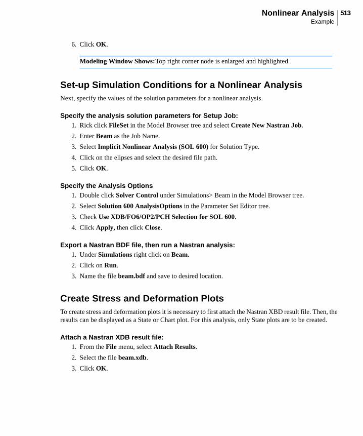
513Nonlinear AnalysisExample
6. Click OK.
Set-up Simulation Conditions for a Nonlinear AnalysisNext, specify the values of the solution parameters for a nonlinear analysis.
Specify the analysis solution parameters for Setup Job:1. Rick click FileSet in the Model Browser tree and select Create New Nastran Job.
2. Enter Beam as the Job Name.
3. Select Implicit Nonlinear Analysis (SOL 600) for Solution Type.
4. Click on the elipses and select the desired file path.
5. Click OK.
Specify the Analysis Options1. Double click Solver Control under Simulations> Beam in the Model Browser tree.
2. Select Solution 600 AnalysisOptions in the Parameter Set Editor tree.
3. Check Use XDB/FO6/OP2/PCH Selection for SOL 600.
4. Click Apply, then click Close.
Export a Nastran BDF file, then run a Nastran analysis:1. Under Simulations right click on Beam.
2. Click on Run.
3. Name the file beam.bdf and save to desired location.
Create Stress and Deformation PlotsTo create stress and deformation plots it is necessary to first attach the Nastran XBD result file. Then, the results can be displayed as a State or Chart plot. For this analysis, only State plots are to be created.
Attach a Nastran XDB result file:1. From the File menu, select Attach Results.
2. Select the file beam.xdb.
3. Click OK.
Modeling Window Shows:Top right corner node is enlarged and highlighted.

Example514
Plot a displacement fringe and deformation plot of beam:1. On the Entity Display Filter toolbar, click Show/Hide All Geometry to turn off the display of
all geometry entities.
2. On the Render toolbar, pull down the finite element display to FE Wireframe.
3. From the Results tab, select Fringe under the Results group.
4. Expand SC1 under Result Cases and select Time = 1:
5. Select Result Type Displacements,Translational.
6. Select Derivation Magnitude.
7. Click Update.
8. Select Deformation as Plot type.
9. Select Result Case Time = 1:
10. Select Result Type Displacements,Translational.
11. Click Update.

515Nonlinear AnalysisExample
12. Using Shift+right mouse button drag to rotate the model to get a view of the deformation.
13. Click Clear.
Plot stress fringees on the beam1. Select Fringe as Plot type.
2. Select Result Case Time = 1:
3. Select Result Type Stress Tensor.
4. For Derivation select von Mises.
5. Click Update.

Example516