Embed Size (px)
Citation preview
Simultaneous recording of EEG and fMRI: New
approach to remove gradient and ballistocardiogram
EEG-artifacts
Dissertation zur Erlangung des akademischen Grades
Doktoringenieur
(Dr. -Ing.)
von Limin Sun
geb. am 16. April 1973 in Jinzhou, Liaoning, China
genehmigt durch die Fakultät für Elektrotechnik und Informationstechnik
der Otto-von-Guericke-Universität Magdeburg
Gutachter:
Prof. Dr.-Ing. Hermann Hinrichs
Prof. Dr.-Ing. habil. Bernd Michaelis
Prof. Dr. rer. nat. habil. Herbert Witte
Promotionskolloquium am 21. Oktober 2009


i
Dedications
This dissertation is dedicated to my family— my parents, my wife, and my daughter. It is
impossible to finish it without their supports.
To my mother, Yan Mu, and my father, Dezhong Sun, who give me a wonderful open and
help me to build the model of life. Especially, mom always encouraged me to finish this
dissertation and help me release the heavy burden of life.
To my wife, Chunling Dong, who is my strength and the purpose of life.
To my daughter, Yijin who brings more fun every day.

ii
iii
Acknowledgments
This thesis was completed during my work as a doctoral student. However, the credit of this
work belongs to not only me but also many other people involved in making it possible.
First of all, I would like to extend my heartfelt gratitude to my perfect advisor, Prof. Dr. -Ing.
Hermann Hinrichs for his encouragement and ongoing kind support. I am also greatly
indebted for his taking much effort and patience in mentoring me to become a qualified
researcher from the method researching to the paper writing. It is indeed his insight and wide
knowledge to guide me to finish the works of this thesis.
I sincerely thank Prof. Dr. -Ing. habil. Bernd Michaelis for being the referee and for his
important suggestions regarding my thesis.
I am indebted to Prof. Dr. med. Hans Jochen Heinze who is the head of the Clinic of
Neurology at the Otto-von-Guericke-University Magdeburg for giving me this chance.
I thank all colleagues in the center of Advanced Imaging who educated me in the technique of
magnetic resonance imaging and in operating the MR scanner. Special thanks to Dr. rer. nat.
Claus Tempelmann for his support regarding imaging questions.
Special thanks also to Dr. Jochem Rieger who taught me EEG and ERP recording.
Finally, I am grateful to our university library for providing all the articles and books needed
for this thesis.

iv
v
List of figures Fig.1.1 EEG recorded outside scanner. ...................................................................................... 2 Fig.1.2 Scanner and structure MRI ............................................................................................ 4 Fig.1.3 EPI and functional MRI ................................................................................................. 5 Fig.1.4 Schematic diagram of artifacts superimposition over EEG........................................... 6 Fig.1.5 EEG-artifacts occurring in an MR environment. ........................................................... 7 Fig.3.1 Schematic diagram of template subtraction................................................................. 12 Fig.3.2 Two artifact examples with different artifact sampling “phases”................................ 13 Fig.3.3 Schematic diagram of BSS-based BCG removal......................................................... 19 Fig.4.1 EPI sequence and gradient artifact............................................................................... 23 Fig.4.2 Watermelon in the scanner serving as a phantom........................................................ 24 Fig.4.3 Example of a typical ERP1........................................................................................... 27 Fig.5.1 Long term fluctuation of artifact observed in the phantom (watermelon) recordings
(position 1). .................................................................................................................. 28 Fig.5.2 Test of slice-specific averaged template conducted with the data recorded with the
phantom (watermelon, position 1, electrode Cz) ......................................................... 30 Fig.5.3 Artifact waveform as recorded in the phantom (watermelon) recordings in four
different positions......................................................................................................... 31 Fig.5.4 Tracking data with different methods: ......................................................................... 32 Fig.5.5 The real case of applying eye-tracker during fMRI scanning...................................... 33 Fig.5.6 Vector representation of true EEG and artifact contaminated EEG (X):..................... 34 Fig.5.7 Estimation the number N used for averaging:.............................................................. 35 Fig.5.8 Evaluation of different weighting profiles. .................................................................. 37 Fig.5.9 Schematic diagram of MAS(old) and MAMAS(new) GAR removal methods........... 39 Fig.5.10 Adjustment of the gradient artifact onsets with respect to the MRI triggers. ............ 40 Fig.5.11 Coordinate systems of the MRI device and of SPM.................................................. 42 Fig.5.12 Examples of SPM-movement indicator and the selection of epochs......................... 42 Fig.5.13 Shape of the digitally simulated gradient artifact waveform. .................................... 44 Fig.5.14 The relationship between st and the sampling interval dt.......................................... 45 Fig.5.15 Alignment without resampling. ................................................................................. 46 Fig.5.16 Residual gradient artifacts to be removed by the special post processing algorithm.48 Fig.5.17 Block diagram of special post processing to remove residual artifacts in case of brief
movements not correctly identified by SPM............................................................. 49 Fig.5.18 The schematic diagram of removing gradient artefacts. ............................................ 50 Fig.5.19 The frequency response of the butterworth bandstop filter applied for removing
vibration artifacts....................................................................................................... 51 Fig.6.1 Schematic diagram of the old BCG removal methods and the new BCG removal
method (such as MNF)................................................................................................. 53 Fig.6.2 The last four MNF-independent components of four subjects. ................................... 60 Fig.6.3 Schematic diagram of extracting the BCG identification signal (BIS)........................ 62 Fig.6.4 The schematic diagram of removing BCG artifacts .................................................... 66 Fig.7.1 Upsampling and resampling: ....................................................................................... 68 Fig.7.2 MAMAS versus MAS: ................................................................................................ 69
vi
Fig.7.3 Comparison of gradient artifacts removal with MAS and MAMAS........................... 70 Fig.7.4 Illustration of the criterion used to select ‘move’ and ‘no move’ segments:............... 71 Fig.7.5 Classification of epochs according to type ‘move’ or ‘no move’ based on the
temporal variation of the SPM related monitor data with 6 sec resolution............... 72 Fig.7.6 Estimation of the amount of residual gradient artifacts (MAS vs. MAMAS) at the
gradient repetition rate and its harmonics for subject nc92 up to 120Hz.................. 72 Fig.7.7 Bar diagram of cumulated spectral coefficients (RINPS-values, i.e. MAS-
MAMAS/MAS )........................................................................................................ 74 Fig.7.8 Special postprocessing:................................................................................................ 75 Fig.7.9 Comparison of different processing steps (as indicated) as applied to one 6-sec-EEG-
segment of subject nc92. ........................................................................................... 79 Fig.7.10 The relative variance vs. number of included components........................................ 80 Fig.7.11 Correlations of the 10 components showing the largest correlation with the BIS..... 82 Fig.7.12 MNF- and ICA-processing of a ten-second EEG data set from subject be98. .......... 83 Fig.7.13 Correlation coefficients vs. number of independent components.............................. 84 Fig.7.14 10-second BCG contaminated EEG example (electrode O1) before processing, after
application of MNF alone, subtraction alone, and combined MNF and subtraction.85
vii
List of abbreviations
EEG Electroencephalogram
BCG BallistoCardioGram
EOG ElectroOculoGram
ECG ElectroCardioGram
MEG Magnetoencephalogram
MR Magnetic Resonance
MRI Magnetic Resonance Imaging
PET Positron Emission Tomography
fMRI functional Magnetic Resonance Imaging
BOLD Blood Oxygenation Level Dependent
EPI Echo Planar Imaging
IFT Inversing Fourier Transformed
TR repetition time
TE echo time
FOV Field of View
AAS Averaged Artifact Subtraction
IAR Image Artifact Reduction
ANC Adaptive Noise Cancellation
RF Radio Frequency
PCs Principle Components
PCA Principal Component Analysis
ICs Independent Components
ICA Independent Component Analysis
SSS Stepping Stone Sampling
FASTR fMRI artifact slice template removal
FIR Finite Impulse Response
SNR Signal to Noise Ratio
RLS Recursive Least Squares
M-RLS Multi-channel Recursive Least Squares
mGLM moving General Linear Model
WT Wavelet Transform
IWT Inverse Wavelet Transform
viii
WNNR Wavelet-based Nonlinear Noise Reduction
JADE Joint Approximate Diagonalization of Eigen-matrices
SPM Statistical Parametric Mapping
BSS Blind Source Separation
SOBI Second Order Blind Inference
MNF Maximum Noise Fraction
MSF Maximum Signal Fraction
INPS Improvement Normalized Power Spectrum
MAS Moving Averaged Subtraction
MAMAS Movement Adjusted Moving Average Subtraction
FID Free Induction Decay
ERP Event Related Potential
VEP Visual Evoked Potential
LPF Lowpass Filter
STD Standard Deviation
LSE Least Square Error
ISI Inter-Slice Interval
DC Direct Current
ADC Analog-to-Digital Converter
LSB Least Significant Bit
PCI Peripheral Component Interconnect
GAR Gradient Artifact
ix
Abstract
Simultaneous recording of the electroencephalogram (EEG) and functional magnetic
resonance imaging (fMRI) may reveal the brain’s activity at high temporal and spatial
resolution. However, the EEG recorded during fMRI scanning is corrupted by large repetitive
artifacts, called gradient artifacts which are generated by the switched MR gradients. In
addition, ballistocardiogram artifacts (BCG) are overlaid on the EEG resulting from heart beat
related body movements and blood flow changes.
To remove the gradient artifacts, several methods have been proposed which subtract
average artifact templates from the ongoing EEG. The most popular version is called ‘moving
average subtraction’ (MAS). In the present thesis, an improvement was developed that
accounts for head movements when averaging the template (this method named ‘movement
adjusted moving average subtraction’ (MAMAS)). After having shown a strong relation
between head movement and artifact waveforms the central point of this algorithm is to track
the head displacements with an eye tracker hardware system or using the SPM (statistical
parametric mapping) software package for cases where a dedicated eye tracker is not
available. Based on the head position of the artifact to be removed, a more precise average
template is achieved by averaging over only those adjacent artifacts observed at the same
head position. To further reduce the residual noise the popular signal-upsampling is replaced
by resampling to synchronize the EEG samples strictly and adaptively with the fMRI timing.
Finally, a new algorithm is introduced to suppress residual artifacts of brief strong movements
which are not reflected by the SPM movement information due to the limited temporal
resolution of the fMRI sequence. In total the new MAMAS algorithm reduces the residual
artifact activity by typically 50% compared to MAS.
For removing BCG artifacts, a new algorithm named maximum noise fraction (MNF) is
introduced and compared with other independent component analysis (ICA) methods. With
the particular ordering feature of MNF (i.e. the decomposed components being ordered by
their signal to noise ratios) most of the BCG artifacts are captured by the last or first
components (depending on the direction of ordering), which is the base to simplify the
complex identification of BCG related ICs. The new approach of combined MNF and a
subsequent average subtraction technique automatically removes the BCG artifacts. It was
evaluated to be efficient both in spontaneous EEG signals as well as in event related
potentials (ERP).
Keywords: EEG, fMRI, MAMAS, gradient artifacts, MNF, BCG artifacts

x
xi
Zusammenfassung
Die simultane Registrierung des Elektroenzephalogramms (EEG) und der funktionellen
Magnetresonanztomographie (fMRT) gestattet die Erfassung der Hirnaktivität mit hoher
zeitlicher und räumlicher Auflösung. Allerdings überlagern sich als Folge der geschalteten
Magnetfeldgradienten der fMRT dem EEG dabei repetitive hochamplitudige und steilflankige
Störsignale (Gradientenartefakte (GAR)). Hinzu kommen ballistokardiographische Artefakte
(BKG) infolge kleiner Körperbewegungen im statischen Magnetfeld des MR Tomographen.
Ein unter dem Namen moving average subtraction (MAS) bekannter Ansatz diente in
dieser Arbeit als Ausgangspunkt für die Entwicklung eines verbesserten Verfahrens zur GAR-
Unterdrückung unter dem Namen movement adjusted moving average subtraction(MAMAS).
MAMAS beobachtet fortlaufend Kopf-Bewegungen, da sich die Form des GAR schon bei
geringen Änderungen der Kopfposition massiv ändert. Eine modifizierte
Augenpositionsüberwachungseinheit, alternativ – mit geringerer zeitlicher Auflösung - ein
Modul des fMRT-Analyseprogramms SPM (statistical parametric mapping), dient zur
Überwachung der Kopfposition, um die Extraktion von Artefakt-Templates aus dem EEG zu
verbessern, indem die Mittelung nur Artefakte einschließt, die bei gleicher Kopfposition
gemessen wurden. Zur weiteren Verbesserung der Artefaktunterdrückung wurde die bisher
übliche massive Abtastratenerhöhung (upsampling) ersetzt durch eine Abtastung an
optimierten Abtastzeitpunkten (resampling), um die EEG-Abtastung mit dem MRT-
Zeitablauf zu synchronisieren. Ein neu entwickelter Algorithmus reduziert verbleibende
Artefakte, die gelegentlich bei sehr kurzen, starken und vom SPM-Monitor nicht korrekt
erfassten Kopfbewegungen auftreten. Insgesamt verringert sich die verbleibende
Artefaktaktivität gegenüber dem MAS-Algorithmus typisch um 50%.
Zur BKG Artefaktunterdrückung wird der ursprünglich zur Bildverarbeitung
entwickelte Algorithmus maximum noise fraction (MNF) eingeführt und mit verschiedenen
independent component analysis(ICA) Methoden verglichen. Dank der Eigenschaft des MNF
Verfahrens, Komponenten nach ihrem Signal-Rausch-Verhältnis zu ordnen, konzentrieren
sich die BKG-bezogenen Komponenten auf die ersten bzw. letzten (je nach Sortierrichtung)
Komponenten, was die Entwicklung eines automatischen Verfahrens ermöglicht. In einem
zweiten Schritt wird durch die Subtraktion gemittelter BKG-Templates (ähnlich MAS) die
verbliebene BKG-Restaktivität weiter reduziert. Abschließend wird die Effizienz des
Gesamtansatzes aus GAR- und BKG-Reduktion durch eine Spektralanalyse des EEG und
zusätzlich durch ereigniskorrelierte Potentiale (ERP) überprüft.

xii
xiii
Contents
Acknowledgments....................................................................................................................iii
List of figures ............................................................................................................................ v
List of abbreviations...............................................................................................................vii
Abstract .................................................................................................................................... ix
Zusammenfassung ................................................................................................................... xi
Contents..................................................................................................................................xiii
Chapter 1 Introduction ............................................................................................................ 1 1.1 EEG .................................................................................................................................. 1 1.2 MRI .................................................................................................................................. 2 1.3 fMRI ................................................................................................................................. 4 1.4 Simultaneous recording of EEG and fMRI ...................................................................... 5
1.4.1 Gradient artifacts and fMRI imaging ........................................................................ 8 1.4.2 Ballistocardiogram artifacts ...................................................................................... 9 1.4.3 Vibration artifacts...................................................................................................... 9
Chapter 2 Aims of the present thesis .................................................................................... 11
Chapter 3 Review of Previous Methods to remove MRI-related EEG artifacts .............. 12 3.1 Gradient artifacts ............................................................................................................ 12
3.1.1 Template Subtraction .............................................................................................. 12 3.1.2 Other approaches..................................................................................................... 16 3.1.3 Conclusion............................................................................................................... 17
3.2 BCG artifacts.................................................................................................................. 18 3.2.1 Blind Source Separation (BSS) (PCA and ICA)..................................................... 18 3.2.2 Other approaches..................................................................................................... 19 3.2.3 Conclusion............................................................................................................... 21
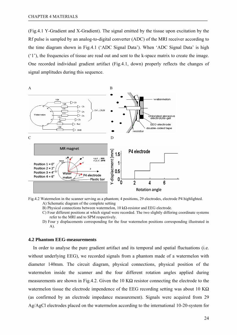
Chapter 4 Materials ............................................................................................................... 23 4.1 fMRI scanning................................................................................................................ 23 4.2 Phantom EEG-measurements......................................................................................... 24 4.3 Human EEG measurements ........................................................................................... 25 4.4 Event related potentials (ERP) ....................................................................................... 27
Chapter 5 New movement adjusted algorithm to remove gradient artifacts ................... 28 5.1 Variations of artifact shape as evaluated by phantom measurements ............................ 28
5.1.1 Long term temporal instability................................................................................ 29 5.1.2 Variability depending on MR-slice ......................................................................... 30 5.1.3 Variations due to electrode movements .................................................................. 30
5.2 Deriving a head movements indicator............................................................................ 31 5.2.1 SPM movement vector: low temporal resolution.................................................... 33 5.2.2 Video-eye-tracker: high temporal resolution .......................................................... 33
5.3 New movement adjusted moving average subtraction (MAMAS) algorithm ............... 34 5.3.1 Basic method of weighted averaged subtraction: Is the residual EEG negligible?. 34 5.3.2 Comparison of different window functions ............................................................ 36 5.3.3 Reduce the influence of head movement by introducing the moving average artifact
................................................................................................................................. 37
xiv
5.3.4 Movement adapted moving averaged subtraction method...................................... 38 5.3.4.1 Detection of gradient artifact onsets................................................................. 39 5.3.4.2 Position dependent artifact averaging. ............................................................. 41 5.3.4.3 New resampling procedure to align sampling time of averaged artifact template...................................................................................................................................... 43 5.3.4.4 Subtraction ....................................................................................................... 47 5.3.4.5 Postprocessing of residual artifacts occurring in case of transient brief movements ................................................................................................................... 48
5.4 The schematic diagram of removing gradient artifacts .................................................. 50 5.5 Removal of vibration artifact by bandstop filtering ....................................................... 51
Chapter 6 New algorithm to remove BCG artifacts ........................................................... 52 6.1 New algorithm based on the Maximum Noise Fraction (MNF) method ....................... 52
6.1.1 Introduction of MNF ............................................................................................... 52 6.1.2 Application of MNF to BCG removal..................................................................... 59 6.1.3 Replacing the adaptive mixing matrix by a fixed matrix to reduce the
computational load .................................................................................................. 61 6.1.4 Separating BCG and EEG: Comparison of MNF to ICA approaches .................... 62
6.2 Additional Moving Average Subtraction algorithm to remove residual BCG activity.. 63 6.3 INPS to evaluate removal performance ......................................................................... 65 6.4 The schematic diagram of removing BCG artifacts....................................................... 66
Chapter 7 Results ................................................................................................................... 67 7.1 Gradient artifacts, MAMAS-algorithm: Evaluation and Comparison with the MAS
algorithm ........................................................................................................................ 67 7.1.1 Gradient artifact resampling.................................................................................... 67 7.1.2 Head motion effect on the reduction of the gradient artifact .................................. 68 7.1.3 The improved performance of using MAMAS ....................................................... 70 7.1.4 Special post processing to reduce residual artifacts caused by brief movements ... 74 7.1.5 Visual evaluation of the new method and comparison with previous methods ...... 76
7.2 BCG artifacts, combined MNF and subtraction algorithm: Evaluation and Comparison........................................................................................................................................ 79
7.2.1 Selection of MNF-components to remove the BCG artifacts ................................. 79 7.2.2 Comparison of MNF, fastICA and JADE: Power to discriminate BCG from EEG80 7.2.3 Reducing the computational load – Usage of a fixed mixing matrix A. ................. 83 7.2.4 Evaluation in the time and frequency domain......................................................... 84
7.2.4.1 Spectral evaluation at the ECG base frequency and its harmonics .................. 84 7.2.4.2 Evaluation in the time domain ......................................................................... 85 7.2.4.3 Total spectrum.................................................................................................. 86
7.2.5 Evaluation with the ERPs........................................................................................ 87
Chapter 8 Discussion.............................................................................................................. 89 8.1 Gradient artifacts ............................................................................................................ 89 8.2 Vibration artifacts........................................................................................................... 95 8.3 BCG artifacts.................................................................................................................. 95
Chapter 9 Summary............................................................................................................... 98
Bibliography ......................................................................................................................... 100
CHAPTER 1 INTRODUCTION
1
Chapter 1 Introduction 1.1 EEG
Richard Caton (1875) discovered electroencephalography (EEG) by a mass of animal
experiments. He found that “feeble currents of varying direction pass through the multiplier
when the electrodes are placed on two points of the external surface, or one electrode on the
grey matter, and one on the surface of the skull.”. Although his finding was the milestone in
the history of monitoring the electrical activity of the brain, the first case of human EEG was
recorded by Hans Berger (1929) in Germany. His reports of human EEG, including studies of
fluctuation of consciousness, first EEG recordings of sleep, the effect of hypoxia on the
human brain, a variety of diffuse and localized brain disorders, and even an inkling of
epileptic discharges, were the greatest contribution in the history of EEG (Ernst Niedermeyer
et al., 1987).
EEG measures the scalp electrical potential which reflects the summed electrical activity of
post-synaptic currents during the physiological and pathophysiological brain activities with
the electrodes placed on the scalp. Consequently, this spontaneous EEG is constantly present
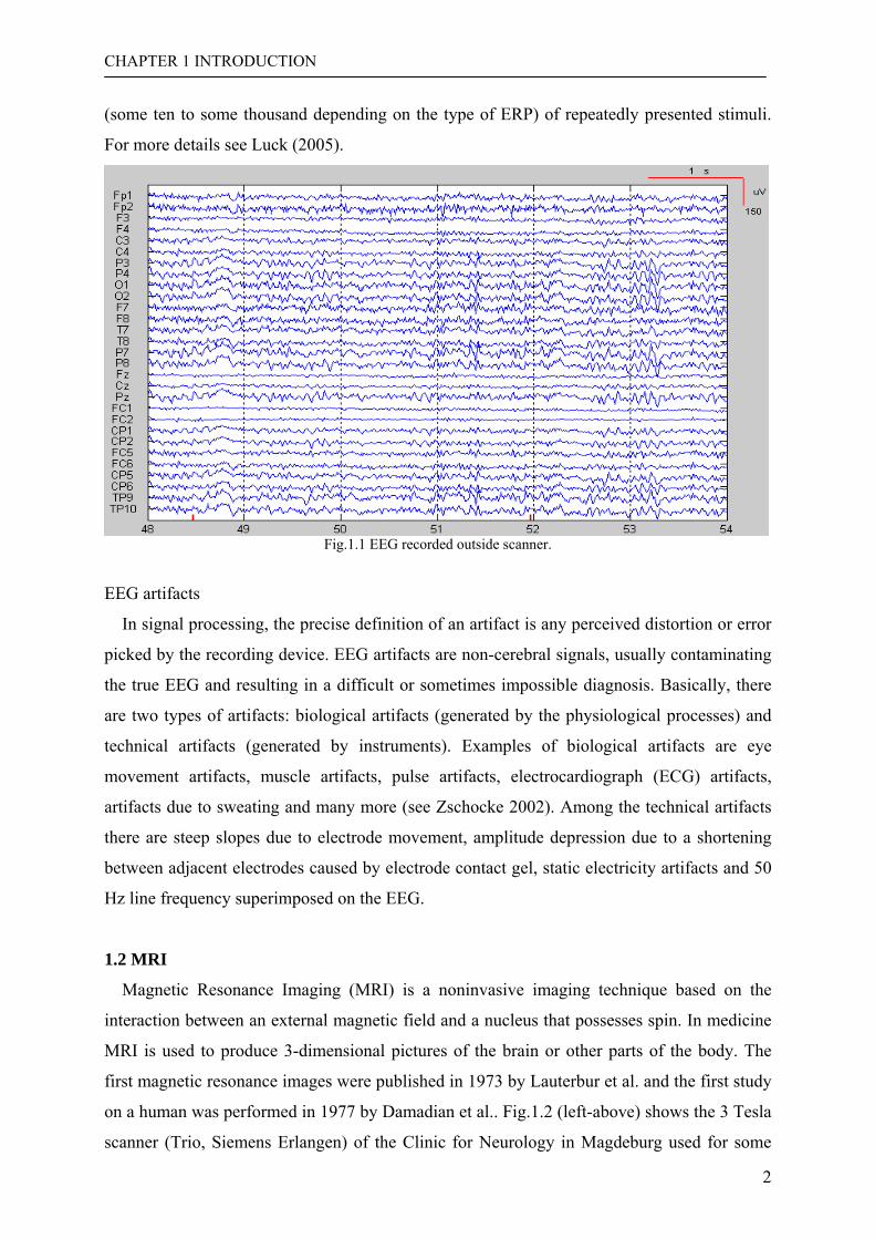
in living humans. A typical EEG of a healthy adult subject is shown in Fig.1.1. According to
the different rhythmic activity (frequency), EEG is divided into different wave patterns such
as delta (up to 4 Hz), theta (4-8 Hz), alpha (8-12 Hz), beta (12-30 Hz) and gamma (30-100
Hz). In medicine the EEG serves as a basic parameter to evaluate the global brain function.
Further medical applications are the diagnosis of epilepsy and sleep staging (see Zschocke
(2002) for further details). Clinical EEG recordings usually include 21channels (in research
up to 256) which are related to a corresponding number of electrodes which are equally
spaced over the whole skull following the international 10-20-system for electrode placement
(Jasper, 1958).
In contrast to the spontaneous EEG the brain generates the specific phasic electrical activity
as a response to external or internal stimulation to the subject. External stimuli are such as the
presentation of a certain pattern on a video screen, a certain acoustic click etc. whereas
internal stimuli reflect mental processes like stimulus processing (for instance detection of a
certain pattern), memory retrieval, word generation etc.. This specific brain response occurs
with a reproducible stimulus-specific waveform and is called ‘event related potential’ (ERP).
In general ERP amplitudes are much below the spontaneous EEG. Therefore, ERPs can only
be extracted from the ongoing EEG using stimulus selective averaging over a large number
CHAPTER 1 INTRODUCTION
2
(some ten to some thousand depending on the type of ERP) of repeatedly presented stimuli.
For more details see Luck (2005).
Fig.1.1 EEG recorded outside scanner.
EEG artifacts
In signal processing, the precise definition of an artifact is any perceived distortion or error
picked by the recording device. EEG artifacts are non-cerebral signals, usually contaminating
the true EEG and resulting in a difficult or sometimes impossible diagnosis. Basically, there
are two types of artifacts: biological artifacts (generated by the physiological processes) and
technical artifacts (generated by instruments). Examples of biological artifacts are eye
movement artifacts, muscle artifacts, pulse artifacts, electrocardiograph (ECG) artifacts,
artifacts due to sweating and many more (see Zschocke 2002). Among the technical artifacts
there are steep slopes due to electrode movement, amplitude depression due to a shortening
between adjacent electrodes caused by electrode contact gel, static electricity artifacts and 50
Hz line frequency superimposed on the EEG.
1.2 MRI
Magnetic Resonance Imaging (MRI) is a noninvasive imaging technique based on the
interaction between an external magnetic field and a nucleus that possesses spin. In medicine
MRI is used to produce 3-dimensional pictures of the brain or other parts of the body. The
first magnetic resonance images were published in 1973 by Lauterbur et al. and the first study
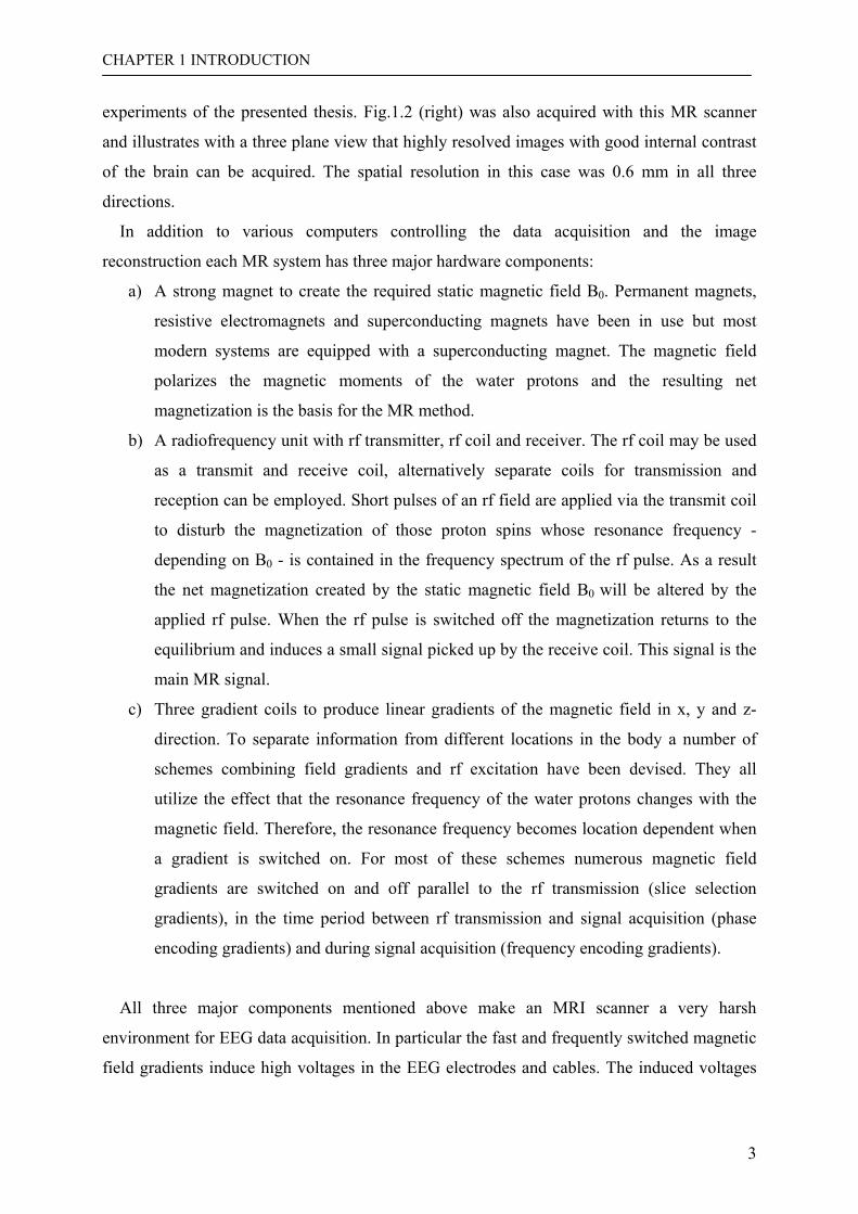
on a human was performed in 1977 by Damadian et al.. Fig.1.2 (left-above) shows the 3 Tesla
scanner (Trio, Siemens Erlangen) of the Clinic for Neurology in Magdeburg used for some
CHAPTER 1 INTRODUCTION
3
experiments of the presented thesis. Fig.1.2 (right) was also acquired with this MR scanner
and illustrates with a three plane view that highly resolved images with good internal contrast
of the brain can be acquired. The spatial resolution in this case was 0.6 mm in all three
directions.
In addition to various computers controlling the data acquisition and the image
reconstruction each MR system has three major hardware components:
a) A strong magnet to create the required static magnetic field B0. Permanent magnets,
resistive electromagnets and superconducting magnets have been in use but most
modern systems are equipped with a superconducting magnet. The magnetic field
polarizes the magnetic moments of the water protons and the resulting net
magnetization is the basis for the MR method.
b) A radiofrequency unit with rf transmitter, rf coil and receiver. The rf coil may be used
as a transmit and receive coil, alternatively separate coils for transmission and
reception can be employed. Short pulses of an rf field are applied via the transmit coil
to disturb the magnetization of those proton spins whose resonance frequency -
depending on B0 - is contained in the frequency spectrum of the rf pulse. As a result
the net magnetization created by the static magnetic field B0 will be altered by the
applied rf pulse. When the rf pulse is switched off the magnetization returns to the
equilibrium and induces a small signal picked up by the receive coil. This signal is the
main MR signal.
c) Three gradient coils to produce linear gradients of the magnetic field in x, y and z-
direction. To separate information from different locations in the body a number of
schemes combining field gradients and rf excitation have been devised. They all
utilize the effect that the resonance frequency of the water protons changes with the
magnetic field. Therefore, the resonance frequency becomes location dependent when
a gradient is switched on. For most of these schemes numerous magnetic field
gradients are switched on and off parallel to the rf transmission (slice selection
gradients), in the time period between rf transmission and signal acquisition (phase
encoding gradients) and during signal acquisition (frequency encoding gradients).
All three major components mentioned above make an MRI scanner a very harsh
environment for EEG data acquisition. In particular the fast and frequently switched magnetic
field gradients induce high voltages in the EEG electrodes and cables. The induced voltages
CHAPTER 1 INTRODUCTION
4
are magnitudes larger compared to the proper EEG signal and good correction algorithms are
a prerequisite for the acquisition of an EEG parallel to the acquisition of MR images.
Fig.1.2 Scanner and structure MRI: Above: Exterior view of the Siemens Trio
system installed in the Clinic for Neurology in Magdeburg.
Right: Example for high resolution structural imaging of the brain.
1.3 fMRI
MRI can not only deliver high resolution images with excellent soft tissue contrast, it can
also be utilized to study the function of many organs; it is for example possible to monitor the
heart in all phases of the heartbeat. Another quite new method called functional Magnetic
Resonance Imaging (fMRI) has become an important method to detect and analyse activities
of the human brain.
The underlying principle was already discovered in 1890 when Roy and Sherrington
indicated that the hemoglobin oxygenation is closely linked to neural activity. However at that
time it was practically impossible to observe the expected changes directly inside the brain.
Later, Pauling and Coryell (1936) elaborated this idea and showed that deoxyhemoglobin is a
paramagnetic particle. On contrary, oxyhemoglobin is diamagnetic and this difference in
magnetic properties causes relaxation times of the MR magnetization to depend on the
oxygen content of the venous blood in the surrounding tissue. The so called blood
oxygenation level dependent (BOLD) fMRI first applied by Seiji Ogawa (1990) and Kenneth
Kwong (1992) exploits the fact that the hemodynamic response overcompensates for the
increased oxygen demands of an active neuronal ensemble and therefore leads to an increase
in oxygen content of venous blood in the vicinity of active brain areas. The change in oxygen
content modulates the strength of the MR signal. Thus, differences in MR signal between
active and passive periods are allowed to identify brain regions involved in the activity. For
CHAPTER 1 INTRODUCTION
5
most fMRI studies it is essential to get the MR data in the shortest time possible. For this
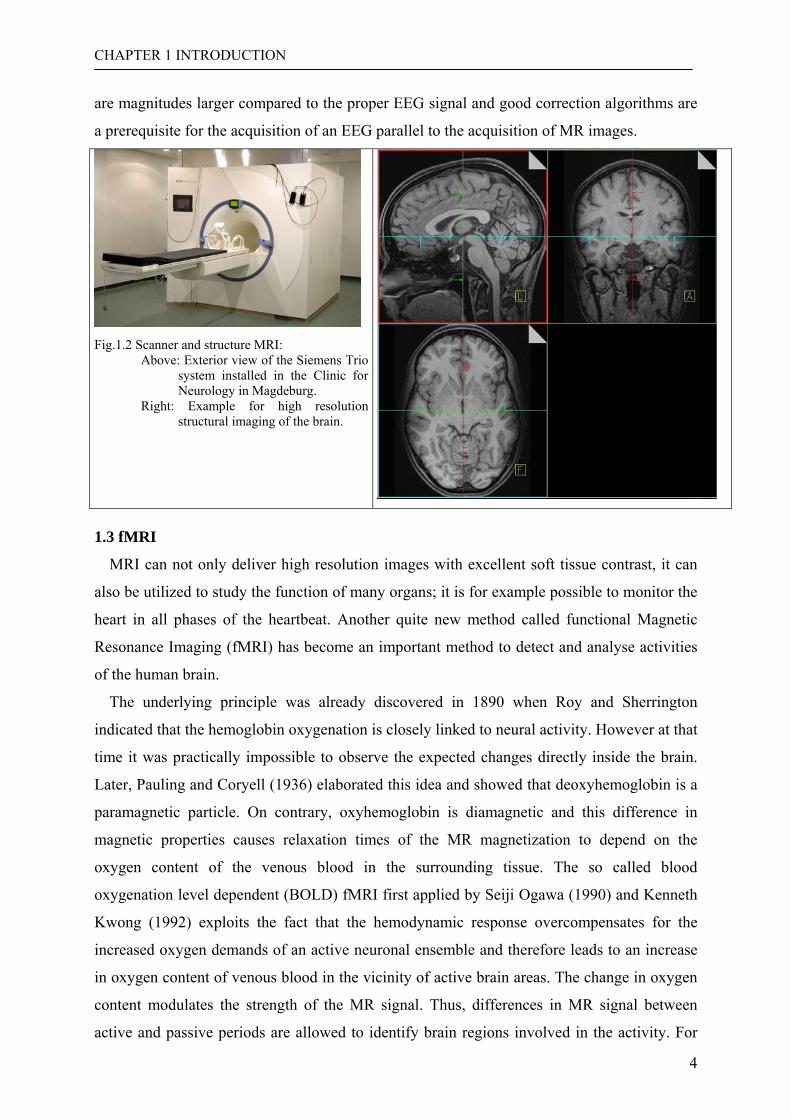
reason, an ultrafast imaging sequence called Echo Planar Imaging is used. As can be seen in
the schematic sequence diagram in Fig.1.3 (above, from Huettel et al.) an EPI sequence
applies particularly fast switching magnetic field gradients and therefore it gives rise to very
strong gradient induced artifacts in the EEG signal if EEG is acquired parallel to the fMRI
data.
Fig.1.3 EPI and functional MRI: Above: Schematic sequence diagram of an EPI sequence (taken from Huettel et al., 2003) typically
applied in fMRI and Bottom: Exemplary low resolution EPI images with overlaid statistical maps indicating brain regions
activated by finger movements of the volunteer, the green rectangle depicts the primary motor cortex.
1.4 Simultaneous recording of EEG and fMRI
Both of EEG and fMRI are used to measure non-invasively brain activity with their own
different features. EEG directly measures the brain activity within a millisecond timescale so
that it can capture neural function at a rather good temporal resolution but with a poor spatial
resolution of a few centimeters for physical reasons (Nunez, 1981). fMRI measures the brain
activity indirectly by the haemoglobin oxygenation changing with excellent spatial few
CHAPTER 1 INTRODUCTION
6
millimeters but a poor temporal resolution of a few seconds. Combining these two methods
provides a high temporal and spatial resolution at the same time.
In practice the combination of both modalities means the simultaneous recording of EEG
and fMRI but also brings the extra artifacts compared with the EEG recording alone. The
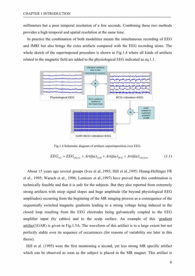
whole sketch of the superimposed procedure is shown in Fig.1.4 where all kinds of artifacts
related to the magnetic field are added to the physiological EEG indicated as eq.1.1.
+
BCG artifacts,related to
the heart beat
Vibration artifacts,due to the
mechanical reasons
+GAR
related to switchedgradient
of MR
Physiological EEG BCG+vibration+EEG
GAR+BCG+vibration+EEG
Fig.1.4 Schematic diagram of artifacts superimposition over EEG.
vibrationBCGGARphysioraw ArtifactArtifactArtifactEEGEEG +++= . (1.1)
About 15 years ago several groups (Ives et al.,1993; Hill et al.,1995; Huang-Hellinger FR
et al., 1995; Warach et al., 1996; Lemieux et al.,1997) have proved that this combination is
technically feasible and that it is safe for the subjects. But they also reported from extremely
strong artifacts with steep signal slopes and huge amplitude (far beyond physiological EEG
amplitudes) occurring from the beginning of the MR imaging process as a consequence of the
sequentially switched magnetic gradients leading to a strong voltage being induced in the
closed loop resulting from the EEG electrodes being galvanically coupled to the EEG
amplifier input (by cables) and to the scalp surface. An example of this ‘gradient
artifact’(GAR) is given in Fig.1.5A. The waveform of this artifact is to a large extent but not
perfectly stable over its sequence of occurrences (for reasons of variability see later in this
thesis).
Hill et al. (1995) were the first mentioning a second, yet less strong MR specific artifact
which can be observed as soon as the subject is placed in the MR magnet. This artifact is
CHAPTER 1 INTRODUCTION
7
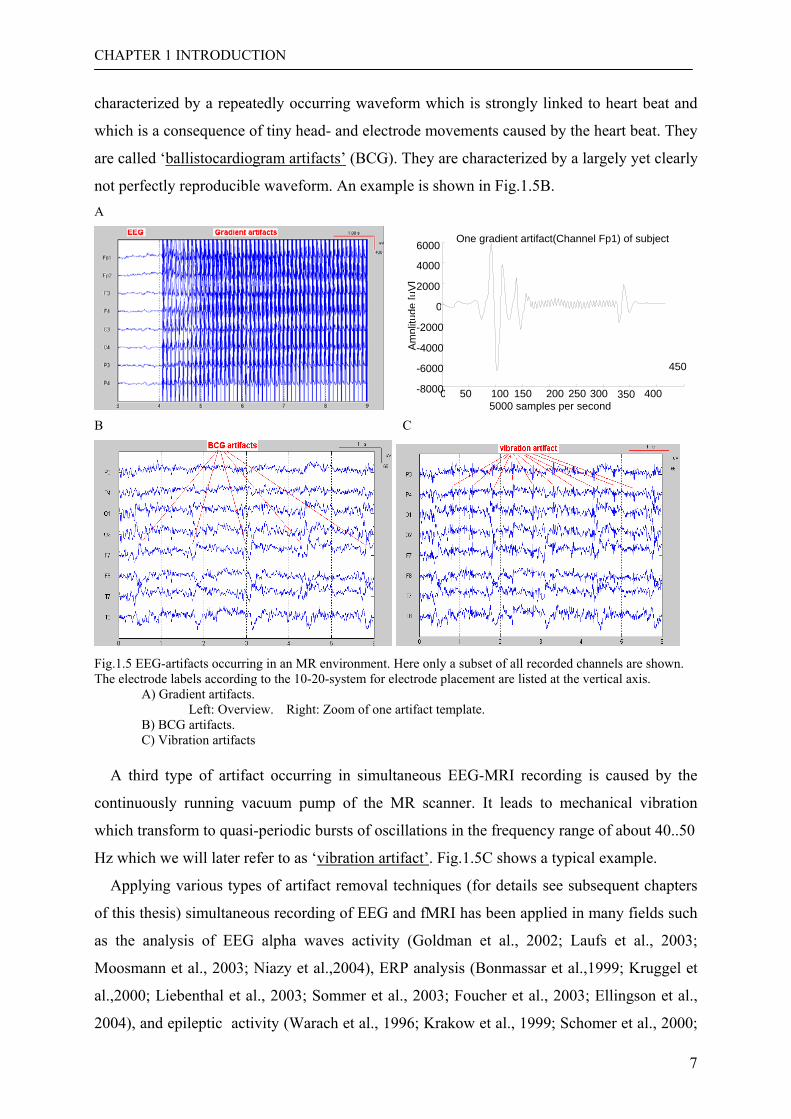
0 50 100 150 200 250 300 350 400-8000
-6000
-4000
-2000
0
2000
4000
6000
5000 samples per second A
mpl
itude
[uV
]
One gradient artifact(Channel Fp1) of subject
450
characterized by a repeatedly occurring waveform which is strongly linked to heart beat and
which is a consequence of tiny head- and electrode movements caused by the heart beat. They
are called ‘ballistocardiogram artifacts’ (BCG). They are characterized by a largely yet clearly
not perfectly reproducible waveform. An example is shown in Fig.1.5B. A
B C
Fig.1.5 EEG-artifacts occurring in an MR environment. Here only a subset of all recorded channels are shown. The electrode labels according to the 10-20-system for electrode placement are listed at the vertical axis.
A) Gradient artifacts. Left: Overview. Right: Zoom of one artifact template.
B) BCG artifacts. C) Vibration artifacts
A third type of artifact occurring in simultaneous EEG-MRI recording is caused by the
continuously running vacuum pump of the MR scanner. It leads to mechanical vibration
which transform to quasi-periodic bursts of oscillations in the frequency range of about 40..50
Hz which we will later refer to as ‘vibration artifact’. Fig.1.5C shows a typical example.
Applying various types of artifact removal techniques (for details see subsequent chapters
of this thesis) simultaneous recording of EEG and fMRI has been applied in many fields such
as the analysis of EEG alpha waves activity (Goldman et al., 2002; Laufs et al., 2003;
Moosmann et al., 2003; Niazy et al.,2004), ERP analysis (Bonmassar et al.,1999; Kruggel et
al.,2000; Liebenthal et al., 2003; Sommer et al., 2003; Foucher et al., 2003; Ellingson et al.,
2004), and epileptic activity (Warach et al., 1996; Krakow et al., 1999; Schomer et al., 2000;
CHAPTER 1 INTRODUCTION
8
Hoffmann et al.,2000; Seeck et al., 2001; Krakow et al., 2001; Salek-Haddadi et al., 2003;
Be´nar et al., 2003; Mirsattari et al., 2004).
1.4.1 Gradient artifacts and fMRI imaging
Echo planar imaging (EPI) has become a popular technique in MR imaging research since
it was proposed as a fast magnetic resonance imaging technique by Peter Mansfield (1977).
EPI is a technique using sequentially switched gradients to read out multiple echoes after just
one rf-excitation thereby substantially reducing the time to collect an image. With respect to
functional brain imaging EPI is the premise for a fast BOLD imaging allowed to collect a full
volume of functional MR images (typically 20 – 30 slices covering the whole brain) within
typically 1 – 2 sec. As described in Section 1.2 a large number of BOLD image volumes is
acquired per experiment (which usually measures the BOLD signal during processing of
external or internal stimuli as described in Section 1.1/ERP) leading to a sequence of switched
gradients with a repetition frequency according to the number of slices/second. The exciting
application of EPI is in the dynamic study of the brain activity with BOLD fMRI discovered
the spatial fluctuation.
Depending on the purpose of study, an fMRI experiment usually lasts from several minutes
to more than hours. Following Faraday’s law of induction each switched gradient (that is,
each slice) leads to a gradient artifact in the EEG. The artifact observed in the EEG thus
summarizes the voltages induced by the various concurrently switched gradients as shown in
Fig.4.1. The resulting template occurs with the frequency as defined by the MR slice time
since the gradients are switched in almost the same manner for each acquired slice.
Several different approaches have been presented to reduce the gradient artifacts. A rather
simple method applies a kind of non linear filtering by setting the artifact related components
of the spectrum (Sijbers et al., 1999; Hoffmann et al., 2000) or directly the waveform (in the
time domain) to zero (Goldman et al., 2000). An alternative method exploits the fact that the
shape of the artifact is largely (yet not perfectly) stable within each EEG-channel but different
between different channels (Hoffmann et al., 2000; Anami et al., 2003; Garreffa et al., 2003).
Given this observation this method subtracts an averaged artifact template from each
individual artifact. This so called ‘averaged artifact subtraction’ (AAS) (Allen et al., 2000)
first uses an interpolation technique to virtually increase the sample rate. Next it averages a
large number of subsequent artifacts as the template which is finally used as the true
waveform to be subtracted.
CHAPTER 1 INTRODUCTION
9
Several variants of AAS have been proposed (see Section 3.1 for an overview). Among
these is a temporally windowed variant named ‘moving averaged subtraction’ (MAS) (Becker
et al., 2005) focussing the averaging process on artifact templates located close to the artifact
to be removed. This was the starting point of that part of the current thesis aiming at an
improved gradient artifact reduction.
1.4.2 Ballistocardiogram artifacts
The ballistocardiogram artifact was already mentioned in the first publication on
simultaneous EEG-MRI recording by Ives et al. (1993). Its amplitudes are in the range of or
slightly larger than typical EEG amplitudes. It can be easily detected visually by its periodic
occurrence according to the heart beat. Ives (1993) has suggested that this artifact results from
the acceleration and abrupt directional change in blood flow in the aortic arch during each
heart beat. Several years later the sources of BCG artifacts have been thought coming from
that “the EEG electrode tiny regular movement on the scalp due to expansion and contraction
of scalp arteries between systolic and diastolic phase, fluctuation of the hall voltage due to the
pulsatile changes of the blood in the arteries and the small cardiac related movements of
head” (Srivastava et al., 2005).
Various methods are found in the literature to remove this kind of artifacts (see Section 3.2
for an overview). Besides subtraction methods (Allen et al., 1998; Müri et al., 1998; Goldman
et al., 2000; Kruggel et al., 2000; Ellingson et al., 2004), several approaches developed for
blind source separation (BSS) have been applied for this purpose, among them are principal
component analysis (PCA) (Negishi et al., 2004; Niazy et al., 2005) and independent
component analysis (ICA) (Be´nar et al., 2003; Srivastava et al., 2005; Briselli et al., 2006;
Nakamura et al., 2006; Debener et al., 2007; Mantini et al., 2007). The present thesis presents
another BSS-method called ‘Maximum Noise Fraction’ (MNF) to achieve a more efficient
BCG reduction.
1.4.3 Vibration artifacts
According to own measurements on three different MR scanners this kind of artifact does
not occur on different scanners with different amplitudes. It was clearly present on the 3T MR
device (for details see Section 4.1) mainly used for this thesis. Vibration artifacts contaminate
the EEG as a consequence of the vibrations originating at the scanner’s vacuum pump
(Briselli et al., 2006). For regular MR usage this pump is continuously running no matter if
the scanner is active or idle. On the 3T MR scanner the amplitude reaches about 200 µV and
CHAPTER 1 INTRODUCTION
10
is thus larger than the normal EEG (10-100 µV). The frequency of this artifact is slightly
fluctuating and mostly extends over a range of 40 Hz to 50 Hz. It can only be suppressed by
either band stop filtering (thereby also loosing a fraction of the underlying EEG) or by
switching the pump off. However, running the scanner with a suspended vacuum pump can
only be accepted for a very limited period and is therefore no regular artifact suppression
technique.
CHAPTER 2 AIMS OF THE PRESENT THESIS
11
Chapter 2 Aims of the present thesis
The aims of the present thesis were:
(i) Analysing the reasons for the residual artifact activity persisting after application of
the existing subtraction methods for gradient artifact reduction, with special emphasis
on the quantification of the effect contributed by head movements.
(ii) Guided by the results of step (i) to develop a new method to improve the reduction of
gradient artifacts with emphasis on high frequencies (beyond 30 Hz), trying to get the
residual artifact down to a level that allows to analyze activity in the γ-frequency band.
(iii) Developing an improved BSS-based BCG removal algorithm that better separates
(iv) Devoloping a fully automatic procedure for BCG removal with more efficient
separation between EEG and BCG activity than existing approaches.
(v) Optimizing the algorithms with respect to computational efficiency.
CHAPTER 3 REVIEW OF PREVIOUS METHODS
12
Chapter 3 Review of Previous Methods to remove MRI-related
EEG artifacts
3.1 Gradient artifacts
The removal of the gradient artifact is challenging given a noise-to-signal ratio of typically
100. The principal goal is to remove as much artifactual activity as possible and at the same
time to keep the true underlying EEG. Besides some other approaches (discussed in Section
3.1.2) the actually most popular subtraction approach (see Section 3.1.1) – which was also
applied in the present thesis - exploits the fact that the gradient artifact’s waveform is largely
stable over time and can thus be removed by subtracting an appropriate waveform (to be
derived from the artifactuous signal) from each artifact in the recorded EEG. Various
realizations of this approach are commercially available as add-on to commercial MR-
compatible EEG recorders (for instance Brain Products, Munich; Neuroscan/Compumedics,
Australia).
Before revisiting existing methods, the terms “epoch” and “template” are defined which are
repeatedly used throughout the subsequent section. An “epoch” is an EEG segment (true
physiological EEG plus artifact) recorded during and starting at the beginning of the MR-
acquisition of one slice. Consequently, the duration of each epoch is TR/N sec with TR
specifying the MRI repetition time (in sec) and N the number of slices per MRI volume. The
artifact “template” is the average over a sequence of subsequent EEG gradient artifacts.
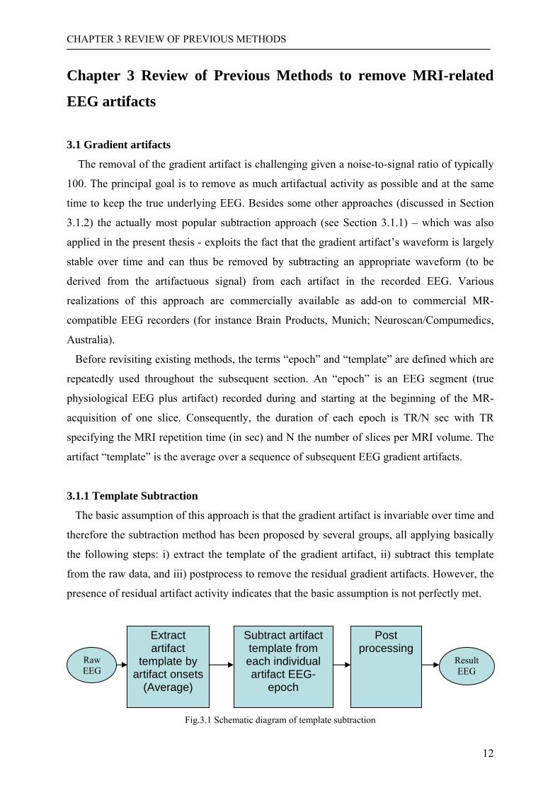
3.1.1 Template Subtraction
The basic assumption of this approach is that the gradient artifact is invariable over time and
therefore the subtraction method has been proposed by several groups, all applying basically
the following steps: i) extract the template of the gradient artifact, ii) subtract this template
from the raw data, and iii) postprocess to remove the residual gradient artifacts. However, the
presence of residual artifact activity indicates that the basic assumption is not perfectly met.
Fig.3.1 Schematic diagram of template subtraction
Extract artifact
template by artifact onsets
(Average)
Subtract artifact template from each individual artifact EEG-
epoch
Post processing
Raw EEG
Result EEG

CHAPTER 3 REVIEW OF PREVIOUS METHODS
13
⎪⎩
⎪⎨
⎧
−≈
−=
∑∞
−∞=i
iGARi
rawclear
ItTGARtGAR
tGARtEEGtEEG
)()(
)()()( (3.1)
where )(tTGARi is the estimated GAR template of the ith epoch at time t and iGARI is the
shifted phase error of the ith epoch. This basic procedure of template subtraction is drawn in Fig.3.1 and the general formula is
described in eq.3.1. All methods with subtraction are based on the same hypothesis, that the
true gradient artifact of one epoch can be estimated by averaging over a number of epochs.
The differences between them only are in the methods of the estimation of the artifact
template and the postprocessing of removing residual gradient artifacts with the same aim of
removing more residual gradient artifacts.
Fig.3.2 Two artifact examples with different artifact sampling “phases”. In the subtraction method, one important factor of influencing the quality of EEG is the
gradient artifacts’ timing error resulting from the asynchronism of EEG sampling and MR-
timing (Fig.3.2). So, although two sampled discrete gradient artifact epochs represent the
same continuous gradient artifact, the timing of the sampling onset respect to the artifact onset
varies giving rise to severe errors if these two epochs are averaged for template extraction
(this timing difference is subsequently called “phase difference”). In order to decrease this
phase error and to further improve the subtraction result, interpolation has to be used to
upsample the signal in order to increase the accuracy of subtraction by aligning the two
gradient artifacts. After interpolation and aligning, downsampling is used to restore the
original sampling rate, which is not only reasonable with respect to subsequent postprocessing
algorithms but also with respect to computer memory required for the algorithm. In the
following, the typical subtraction method is outlined in more detail. Besides the artifacts
stable waveforms all of these algorithms assume (i) that the underlying true EEG is not
correlated with the superimposed artifact and (ii) that the EEG has zero mean. The second
CHAPTER 3 REVIEW OF PREVIOUS METHODS
14
assumption does not restrict the general application of these methods since either the
amplifier has a non-zero lower cut off frequency (thereby suppressing a potential DC offset)
or the non-zero mean can be determined and subtracted before any processing).
The typical subtraction method comprises the following steps: 1. Upsample and align each gradient artifact by interpolation. 2. Estimate the artifact template by averaging over a set of M artifact epochs with M as well as the type of
averaging varying over the different approaches proposed so far. 3. Subtract this template from each gradient artifact. 4. Downsample the result. 5. Postprocess to remove residual gradient artifacts.
Allen (2000) was the first to present the averaged artifact subtraction (AAS) method. He
extracted the artifact template by averaging over all artifacts observed in the current
recording. Resiudal artifact activity remaining after AAS was reduced by an adaptive noise
cancellation (ANC) technique which was guided by a MR slice timing trigger signal.
Upsampling to 100 KHz frequency was accomplished by a 25-coefficientsinc interpolation
(up to 50KHz). A unique artifact template was extracted by averaging over the first 25 artifact
epochs and subsequently subtracted from all artifact epochs of the recording. This method still
leaves a residual artifact of about 10 µV (Allen, 2000) and potentially removes some fraction
of the underlying true EEG since the effect of the ANC with respect to the EEG cannot be
controlled. Furthermore, the sinc algorithm applied for interpolation is time consuming.
Another variant of the subtraction method was proposed by Be´nar et al. (2003) who
concentrated on the asynchronismof EEG sampling and MR timing. To get around this
problem they used several different artifact templates which were generated by averaging
over several groups of artifact epochs. Each group included only artifact epochs showing the
same lag (as determined by cross correlation) with respect to a reference epoch (usually the
first one). The reference epoch and each epoch were interpolated and upsampled by a factor
of 10 to refine the lags. Then, each averaged template was only averaged over all epochs in
the corresponding group. Finally, the subtraction was performed using the template best
matching the artifact epochs in terms of its lag.
The real-time artifact filter (Garreffa et al., 2003) brought the artifact removal technique
into another new development direction (real-time processing) with the assumption of the
averaged artifact template for each individual artifact being long term stable. This approach in
effect represents a non linear online filter algorithm. First the waveform of the averaged
artifact template is defined by the initial 48 seconds data. Next this template is used for the
peak detection algorithm to locate the onsets of artifacts by correlation. Then the procedure of
subtraction is performed as a real-time process. Additional filters are applied to reduce the
CHAPTER 3 REVIEW OF PREVIOUS METHODS
15
residual noise. This algorithm requires a powerful computer to meet the computational
demands of the real time processing.
An approach called ‘stepping stone sampling’ (SSS) (Anami et al., 2003) achieves a higher
signal-to-artifact ratio by (i) strictly synchronizing the EEG sampling with the MR timing and
(ii) by modifying a standard fMRI measurement sequence so that EEG sampling might be
performed at every 1000 µs (i.e. digitization rate 1000 Hz) exclusively in the period in which
the gradient artifact resided around the baseline level. Since the gradient artifact isn’t
perfectly zero at the time of EEG sampling some gradient related activity can still persist but
with an amplitude much below (by a factor < .1) amplitudes observed with standard fMRI
settings. The remaining residual artifacts are subsequently removed with the subtraction
technique. In this realization the template was extracted by averaging over all artifact epochs
of the recording.
Becker et al. (1005) introduced the ‘weighted moving averaged subtraction’(MAS) method
which accounts for temporally varying artifact waveforms by applying a weighted moving
average scheme to extract an individual artifact template for each artifact to be removed.
Before this processing step the signals are upsampled to 50 KHz by cubic spline interpolation,
aligned by cross correlation and finally downsampled to the original 5 KHz sampling rate.
The weighting function has an exponential profile and extends over 120 epochs. After the
subtraction step, a bandpass filter of 0.53-70 Hz is applied as to remove the residual noises.
However, according to own test of this method, residual artifacts are still a problem in case of
head motion.
‘FMRI artifact slice template removal’ (FASTR) (Niazy et al., 2005) combines a local
moving artifact template subtraction with subsequent applications of PCA and ANC to
remove the residual artifacts. Each epoch is upsampled to 20 KHz with since interpolation
and realigned with all other epochs. Beyond the mere artifact subtraction this algorithm relies
on a PCA to capture residual artifact activity caused by temporal artifacts variations. The
ANC was applied according toe the method described by Allen (2000) to remove any
remaining residual components (not captured in PCA). The problem with this approach is that
there is no strict rule to determine the appropriate number of PCA components to be
suppressed (that is to find a compromise between removing the artifact and keeping the true
underlying EEG).
Recently, a variant of the average-subtraction method was proposed (Goncalves et al.,
2007a; Goncalves et al., 2007b) to correct the temporal misalignment between EEG and fMRI
data by estimating three MR sequence timing parameters in terms of the EEG recorder’s time
CHAPTER 3 REVIEW OF PREVIOUS METHODS
16
base (before any subtraction processing). The estimated parameters are: the MR sequence
repetition time TREEG, the time between the beginning of the MR-volume acquisition and the
acquisition of the first slice DT, and the acquisition time of one slice (i.e. the slice time)ST.
Next, the shifts needed for an optimal temporal alignment are derived from these three
parameters. Then, the alignment is performed by a resampling procedure applying a FFT
based interpolation scheme. Second, after these sub-sample shifts, separate templates are
derived for each slice within the MR volumes and an additional template is determined
averaging over these slice specific templates of volumes. Finally, the slice template and the
volume template are combined and subtracted from each epoch.
3.1.2 Other approaches
Besides subtraction, there are two different methods working without any subtraction. One
of them is called ‘frequency removing method’ (Hoffmann et al., 2000) which eliminates all
artifact related frequency components outside the clinically relevant frequency window of the
EEG (0.1–40 Hz) by high- or low-pass filters. Components below 40 Hz are removed by
employing a series of band-stop filters. This method necessarily causes a loss of information
of the true underlying EEG below 40 Hz frequency. A similar method has been proposed by
(Goldman et al., 2000) for the time domain which sets all artifactuous epochs of the ongoimg
EEG to zero. Although it is not hard to locate the gradient artifacts, there are two obvious
disadvantages: i) the scanning frequency must be low (such as 4 slices per second) in order to
save a sufficient fraction of the EEG as not being suppressed, and ii) the processed EEG data
is fractioned in to usable and non usable parts.
A more sophisticated filtering approach was developed by Sijbers et al. (1999) aiming at
keeping as much EEG as possible. This technique, called ‘adaptive restoration scheme’,
applies a non-linear filter as follows: First the spectrum of the artifact template is estimated by
averaging over a number (15 for slow MR sequences to 31 for faster ones) of spectra of
gradient artifacts detected by MR triggers. A scaled version of this average spectrum is
subsequently subtracted from each of the artifact epochs whereby the scaling parameter is set
to minimize the difference between the two spectra. The resulting difference spectrum is
finally transformed back to the time domain thereby yielding the EEG signal. At the same
time, the average artifact spectrum is updated to track potential changes of the artifact
template. The problem with this method is that the amount to which the true EEG is
influenced by this processing cannot be controlled.
CHAPTER 3 REVIEW OF PREVIOUS METHODS
17
Negishi et al. (2004) – after realignament of the artifacts - applied a PCA to the EEG to
identify principal components (PC) mainly carrying artifact activity. An artifact template of
each epoch is then computed as a linear combination of these PCs (details regarding the
calculation of the weighting factors are found in Negishi et al., 2004). Finally these combined
PCs are subtracted from the original epoch. The resulting signal is smoothed with an 80Hz
lowpass filter.
Yet another method, (Wan et al., 2006b) estimated each gradient artifact epoch by a band-
limited Taylor expression assuming that each gradient artifact can be defined as a linear
combination of the average artifact template and its derivatives with the linear coefficients
varying over the epochs. These varying coefficients are fitted by a least square error (LSE)
algorithm minimizing the sum of squares of the differences between the epoch and the
estimated epoch. After convergence of the LSE and subtraction of the estimated epoch an 8-
order Butterworth lowpass filter (LPF), with a cut-off frequency of 70 Hz, removes the
residual noise. According to Wan et al. (2006b) this approach is comparable to an adaptive
finite impulse response (FIR) filter. The analyses of Wan et al. (2006b) also demonstrated the
temporal instability of the gradient artifact template. It is hard to compare the removal effect
of the techniques to other approaches since Wan et al. did not apply any interpolation and
upsampling technique.
Finally, Mantini et al. (2007) applied AAS as the first processing stage but subsequently
applied an ICA to capture and suppress specific independent components carrying residual
artifact activity.
3.1.3 Conclusion
Summarizing the approaches published so far and taking into account the practice of many
imaging labs (which mostly use commercially available artifact suppression programs),
template subtraction is by far the most popular technique to remove gradient artifacts. All of
them upsample the signal as a premise for an appropriate alignment of the artifact epochs. The
main difference between the various algorithms is the way they determine the template to be
subtracted. In all cases some residual activity remains after subtraction. Some of them reduce
it by application of a PCA or ICA technique after the subtraction, but all of them finally
smooth the data using a low pass filter. So far the reason for some residual artifact activity
persisting after processing has not been sufficiently identified.
CHAPTER 3 REVIEW OF PREVIOUS METHODS
18
3.2 BCG artifacts
3.2.1 Blind Source Separation (BSS) (PCA and ICA)
BCG artefacts are less reproducible than gradient artifacts, so that the subtraction method
won’t work as efficiently. Thus the research is focussed on the othogonality of the true EEG
and the BCG artifacts. From a statistical perspective ‘orthogonality’ between two signals
means that they are not correlated, i.e. each varying separately. Principal component analysis
(PCA) is one of the standard methods to separate such orthogonal components. The basic idea
is to identify and suppress those principal components (PC) which mostly capture artifact
activity so that the amount of EEG lost after suppression can be neglected. Negishi et al.
(2004) and Niazy et al. (2005) proposed this concept to remove BCG artifacts (as the second
step after gradient artifact removal, see above). In principle they subtracted a linear
combination of some PCs from the signal, including all PCs (Negishi et al., 2004) or a limited
number (Niazy et al., 2005) explaining the largest amount of the total variance. Independent
component analysis (ICA) is a different BSS-approach which tries to identify statistically
independent (rather than orthogonal) components within a composite signal. With respect to
BCG removal the problem with any ICA procedure is that components resulting from the
PCA or ICA analysis are randomly ordered regarding the amount of artifact activity captured
by each component. This hampers an automatic procedure to identify components which
should be suppressed for artifact removal. Thus, the identification of BCG ICs reflects an
important key aspect, especially with respect to automated removal algorithms. At the
moment there are two kinds of methods: interactive processing (i.e. visually selecting the
relevant ICs) (Be´nar et al., 2003) and fully automatic processing (Srivastava et al., 2005). For
the semi-automatic processing, the BCG ICs have to be visually identified by an observer
(human, not computer) which consequently introduces a man caused factor increasing the
likelihood of either distorting the underlying EEG (if too many ICs are removed) or leaving
too much residual artifacts (if a too low number or a wrong choice of ICs is removed ICs).
For the automatic processing, a rule is needed guiding the selection of BCG related ICs
automatically. Usually, the electrocardiogram (ECG) is recorded simultaneously with the
EEG as an additional reference channel. Basically, Srivastava et al. (2005) accomplish the
BCG removal task in five steps: i) Decomposing the original EEG into different ICs (i.e.
application of the ICA), ii) Computing the correlation coefficient between the ECG and each
IC, iii) Choosing those ICs with high correlation coefficient as BCG-related ICs and setting
them to zeros, and iv) reconstructing the underlying EEG by recombining the remaining non-
zero ICs.
CHAPTER 3 REVIEW OF PREVIOUS METHODS
19
Briselly et al. (2006) refined the ICA approach by running it multiple times having in mind
the idea of reducing the BCG residuals more and more with an increasing number of
iterations.
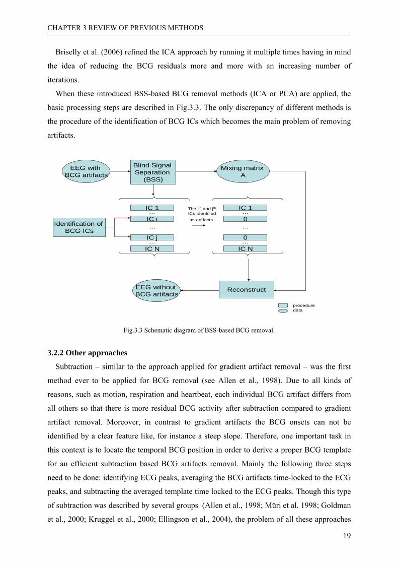
When these introduced BSS-based BCG removal methods (ICA or PCA) are applied, the
basic processing steps are described in Fig.3.3. The only discrepancy of different methods is
the procedure of the identification of BCG ICs which becomes the main problem of removing
artifacts.
Blind Signal Separation
(BSS)
IC 1
IC N
IC i...
...
Mixing matrixA
Identification of BCG ICs
IC j
...
IC 1
IC N
0...
...0
...
Reconstruct
EEG withBCG artifacts
EEG withoutBCG artifacts
: procedure: data
The ith and jthICs identifiedas artifacts
Fig.3.3 Schematic diagram of BSS-based BCG removal.
3.2.2 Other approaches
Subtraction – similar to the approach applied for gradient artifact removal – was the first
method ever to be applied for BCG removal (see Allen et al., 1998). Due to all kinds of
reasons, such as motion, respiration and heartbeat, each individual BCG artifact differs from
all others so that there is more residual BCG activity after subtraction compared to gradient
artifact removal. Moreover, in contrast to gradient artifacts the BCG onsets can not be
identified by a clear feature like, for instance a steep slope. Therefore, one important task in
this context is to locate the temporal BCG position in order to derive a proper BCG template
for an efficient subtraction based BCG artifacts removal. Mainly the following three steps
need to be done: identifying ECG peaks, averaging the BCG artifacts time-locked to the ECG
peaks, and subtracting the averaged template time locked to the ECG peaks. Though this type
of subtraction was described by several groups (Allen et al., 1998; Müri et al. 1998; Goldman
et al., 2000; Kruggel et al., 2000; Ellingson et al., 2004), the problem of all these approaches
CHAPTER 3 REVIEW OF PREVIOUS METHODS
20
is the considerable residual BCG activity remaining due to the BCG artifact’s temporal
instability (according to own empirical tests).
A different algorithm was developed by (Bonmassar et al., 1999) who designed a linear
spatial filter to recover the BCG artifacts contaminated EEG directly, however, exclusively
focussing on the processing and extraction of visual evoked potentials (VEP). In principle this
method tries to maximize the signal to noise ratio by the well known generalized maximum
eigenvalues of the signal covariance matrix and the noise covariance matrix. The noise
covariance matrix is estimated from all VEP epochs recorded during fMRI by subtracting the
averaged VEP as recorded outside the scanner, whereas the signal covariance matrix is
estimated by using epochs recorded outside the scanner without any subtraction. Although
this method does not need to record an extra ECG, it is time consuming since it requires extra
EEG data (including visual stimulation) recorded outside the scanner as the base to compute
the two signal-to-noise ratio values.
The adapter filter technique by Sijbers et al. (2000) is based on a average-subtraction
method extended by the following features: An improved detection of QRS waves, the
estimation of the BCG artifact template by means of wavelets, and a filter which is
continuously adapted to the ongoing BCG epochs. To detect QRS onsets, a band-pass filter
was first applied to remove irrelevant information. Second, local maxima within an interval of
0.5 seconds were retained and subjected to a selection criterion applying constraints on the
distance between subsequent maximum values. The BCG artifact template was estimated by
median-filtering a number of the wavelet filtered artifacts. Given this primary template, the
final adaptive filtering procedure proceeds as follows: the template is updated with each new
artifact guided by criterion of minimizing the difference between the template and the actual
artifact. Another adaptive filter version was applied by Bonmassar et al. (2002), who used a
piezo based motion sensor to pick up head movements and evaluate it in terms of an adaptive
noise cancellation method to suppress any kind of motion related artifacts including the BCG.
This procedure was applied to remove BCG artifacts in the context of an interleaved
EEG/fMRI recording protocol with alternating periods of active EPI scanning and non-
scanning. The relationship between the noise (artifacts) and the motion sensor signal is
modeled linearly using a time-varying finite impulse response (FIR) kernel which is
adaptively updated with kalman filter algorithm.
Kim (2004) suggested to combine the average template subtraction with a noise reduction
approach using a wavelet decomposition (i.e. wavelet transform, selective suppression of
some wavelet scales and finally inverse transform) and finally with an adaptive recursive
CHAPTER 3 REVIEW OF PREVIOUS METHODS
21
least-square (RLS) eliminating remaining residual artifactual activity. For a successful
application this method needs two ECG channels guiding the template extraction process.
Wan et al. (2006a) used a similar wavelet decomposition technique but combined it with a
nonlinear noise reduction originally developed by Grassberger et al. (1993) as a general
denoising concept derived from chaos theory. Residual artifact activity remaining after this
procedure is removed by subtracting a BCG template derived by spatially averaging (guided
by the ECG) over all EEG channels. According to Wan et al. (2006a) this ‘Wavelet-based
Nonlinear Noise Reduction’ (WNNR) is computationally very demanding making it less
suitable for routine applications. In addition – similar to most of the above described methods
– potential distortions of the ongoing spontaneous EEG cannot be controlled.
The template subtraction approach was substantially extended by Vincent et al. (2007) with
respect to the observation that the BCG waveform substantially fluctuates over time, and is
usually longer than the heart beat interval leading to overlap effects. To include points the
authors defined a three-dimensional BCG template (i.e. a multichannel template) and
estimated by a ‘moving general linear model’ (mGLM) which estimates the coefficients of the
Fourier transform of the template. This estimated 3D-template is finally time locked to the
ECG-subtracted from the signal. Despite its advantages in handling overlapping BCG artifacts
this method is primarily suited to research EEG recordings (Vincent et al., 2007) since it
requires substantial user interactions which is not acceptable under clinical routine conditions.
The ‘multi-channel Recursive Least Squares (M-RLS) algorithm proposed by Masterton et al.
(2007) includes four extra channels representing the head motion. These non-physiological
signals are used for an adaptive BCG template estimation (similar to the method of
Bonmassar, 1999) which is subsequently subtracted to remove the BCG artifact as well as
arbitrary other movement artifacts. With respect to clinical EEG recordings this method is
hampered by the need of extra wires to be connected to the head and extra electronics to
record the motion signals
3.2.3 Conclusion
Due to the temporal variability of the BCG artifact waveform the artifact subtraction
approach (like AAS) as developed for gradient artifact removal cannot be applied here.
Instead, several groups have extended AAS using algorithms allowing for an adaptive
estimation and modification of the artifact template. However, the majority of published
papers replaced the template subtraction by a spatiotemporal approach applying blind source
separation (BSS) techniques like PCA and ICA. Though being successfully applied under a
CHAPTER 3 REVIEW OF PREVIOUS METHODS
22
wide range of research and routine conditions the problem with these techniques is that- due
to the missing orthogonality between the artifact and the EEG signals - it cannot be controlled
how much of true EEG is lost after suppression of components mainly (but not exclusively)
carrying for artifact activity. Furthermore, most of the proposed algorithms are not suited for
an automatic procedure since they require a user interaction.
CHAPTER 4 MATERIALS
23
Chapter 4 Materials 4.1 fMRI scanning
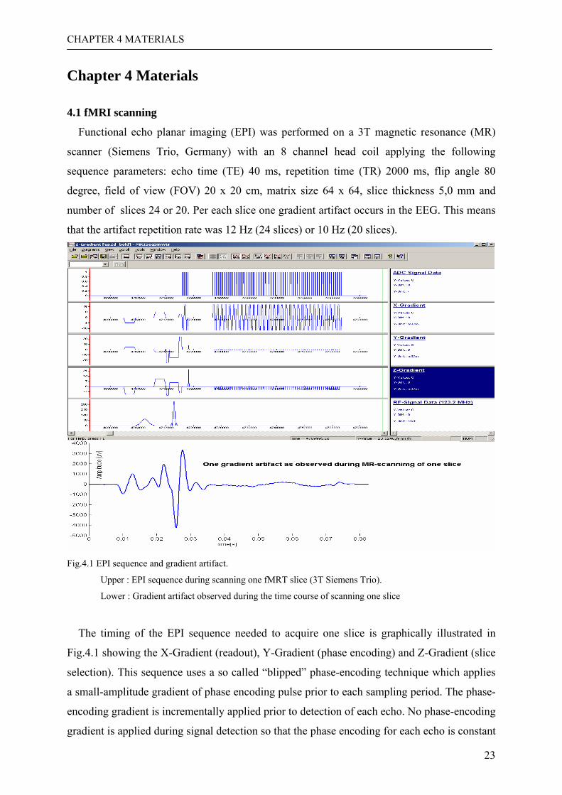
Functional echo planar imaging (EPI) was performed on a 3T magnetic resonance (MR)
scanner (Siemens Trio, Germany) with an 8 channel head coil applying the following
sequence parameters: echo time (TE) 40 ms, repetition time (TR) 2000 ms, flip angle 80
degree, field of view (FOV) 20 x 20 cm, matrix size 64 x 64, slice thickness 5,0 mm and
number of slices 24 or 20. Per each slice one gradient artifact occurs in the EEG. This means
that the artifact repetition rate was 12 Hz (24 slices) or 10 Hz (20 slices).
Fig.4.1 EPI sequence and gradient artifact.
Upper : EPI sequence during scanning one fMRT slice (3T Siemens Trio).
Lower : Gradient artifact observed during the time course of scanning one slice
The timing of the EPI sequence needed to acquire one slice is graphically illustrated in
Fig.4.1 showing the X-Gradient (readout), Y-Gradient (phase encoding) and Z-Gradient (slice
selection). This sequence uses a so called “blipped” phase-encoding technique which applies
a small-amplitude gradient of phase encoding pulse prior to each sampling period. The phase-
encoding gradient is incrementally applied prior to detection of each echo. No phase-encoding
gradient is applied during signal detection so that the phase encoding for each echo is constant
CHAPTER 4 MATERIALS
24
(Fig.4.1 Y-Gradient and X-Gradient). The signal emitted by the tissue upon excitation by the
Rf pulse is sampled by an analog-to-digital converter (ADC) of the MRI receiver according to
the time diagram shown in Fig.4.1 (‘ADC Signal Data’). When ‘ADC Signal Data’ is high
(‘1’), the frequencies of tissue are read out and sent to the k-space matrix to create the image.
One recorded individual gradient artifact (Fig.4.1, down) properly reflects the changes of
signal amplitudes during this sequence.
A B
C D
Fig.4.2 Watermelon in the scanner serving as a phantom; 4 positions, 29 electrodes, electrode P4 highlighted.
A) Schematic diagram of the complete setting B) Physical connections between watermelon, 10 kΩ-resistor and EEG electrode. C) Four different positions at which signal were recorded. The two slightly differing coordinate systems
refer to the MRI and to SPM respectively. D) Four y displacements corresponding for the four watermelon positions corresponding illustrated in
A).
4.2 Phantom EEG-measurements
In order to analyse the pure gradient artifact and its temporal and spatial fluctuations (i.e.
without underlying EEG), we recorded signals from a phantom made of a watermelon with
diameter 140mm. The circuit diagram, physical connections, physical position of the
watermelon inside the scanner and the four different rotation angles applied during
measurements are shown in Fig.4.2. Given the 10 KΩ resistor connecting the electrode to the
watermelon tissue the electrode impendence of the EEG recording setting was about 10 KΩ
(as confirmed by an electrode impedance measurement). Signals were acquired from 29
Ag/AgCl electrodes placed on the watermelon according to the international 10-20-system for
CHAPTER 4 MATERIALS
25
electrode placement (Jasper, 1958) and were identical to the real human EEG recordings, see
next section. The whole phantom EEG recording consisted of four runs, each of 10 min
duration (according to 300 MR volumes) while the MR scanner acquired images. Between
each run, the watermelon was rotated by about 2° around the x axis (see Fig.4.2) while
keeping the same position. To prevent any motion during the measurement the melon was
fixed by support jaw. Hence the watermelon only simulated a head motion in one direction
thus simulating a subject moving its head during scanning. As shown in Fig.4.2D the
displacement of the P4 electrode per rotation step was about 0.5 mm in the vertical (i.e. y)
direction resulting from a 2.4 mm displacement in tangential direction which is comparable to
a realistic strong head movement.
The idea to run the watermelon experiment was to record the pure gradient artifact without
any additional BCG artifact and without any EEG. This provided the opportunity to uncover
both to analyze the relationship between the electrode position and the gradient artifact’s
waveform and the temporal stability of the artifact. The 10 KΩ antimagnetic resistance
(DALE CMF55 10K .1%T9 0410) was connected between the water melon and EEG
electrodes in order to simulate a real measurement situation. Those electrodes were fastened
with double-sided tapes.
4.3 Human EEG measurements
Six volunteers (five male and one female, average age 25, range 20-27 years) participated
in the study. Four subjects(three male and one female) were requested to keep their head
motionless as good as possible during the recording when seeing a series of pictures (see next
subsection). The other two subjects (male) were asked to slightly move their heads according
to the different types of picture. In two of the subjects the head movements were recorded
online with high temporal resolution (20 ms) applying a video-based device developed by the
Magdeburg MR-group (Kanowski et al., 2007), for details see chapter 5.2.2. These recordings
served to check the quality of the offline head movement information derived from the MR-
image sequence by the statistical parametric mapping (SPM) analysis program with a
resolution of 1 sec, for details see chapter 5.2.1.
The EEG was recorded using a BrainAmp MR-Plus MR-compatible EEG-amplifier (Brain-
Products, Germany). In each subject the EEG was obtained under the three different
conditions: (i) Inside the scanner concurrent to BOLD-imaging according to section 4.1.
These recordings contain both gradient and BCG artifacts. (ii) Inside the scanner but without
BOLD-scanning. These EEG-recordings can be expected to show only BCG artifacts. (iii)
Outside the scanner room thereby providing EEG recordings without any scanner specific
CHAPTER 4 MATERIALS
26
artifacts. These recordings served as a reference for the artifact correction developed in this
work.
Generally, each EEG data set consisted of a continuous recording of 10 minutes duration
applying the following acquisition parameters: Analog bandpass filtering with cut off
frequencies of 0.0016 Hz and 250 Hz respectively, sampling rate per channel 5 kHz, 16 Bit
digital resolution with the least significant bit (LSB) representing 500 nV resulting in a
dynamic range of ± 16 mV. The amplifier and digitizer box was located close to the subjects’
head (distance about 1 m). After digitization the EEG data were transferred out of the shielded
magnetic resonance (MR) cabin by a fiber optic cable to a digital signal collecting card
(Peripheral Component Interconnect (PCI) bus) of a personal computer (PC) located outside
the shielded room. As empirically analysed, the amplifier noise level with grounded input was
1uV (standard deviation (STD)) at the bandwidth specified before. Inside the scanner room,
the EEG amplifier box was fixed with band to prevent additional artifacts due to amplifier
movements. The power of the amplifier/digitizer box was supplied by a rechargeable Li-
battery. Thirty-four electrodes (Ag/AgCl) were placed on the scalp: Twenty-nine electrodes
(Fp1, Fp2, F3, F4, C3, C4, P3, P4, O1, O2, F7, F8, T7, T8, P7, P8, Fz, Cz, Pz, FC1, FC2,
CP1, CP2, FC5, FC6, CP5, CP6, TP9, TP10 according to the international 10-20-system
(Jasper 1958) plus some extensions according to the 10-10-system (Chatrian et al., 1985) used
to record EEG data for four of the six subjects. All these electrodes were applied using a
textile cap holding the electrodes (‘electrode cap’). A further electrode was placed near the
right eye to record the electrooculogram (EOG). Two additional electrodes were placed at the
subjects back close to the superior and inferior end of the heart to pick up two
electrocardiogram (ECG) signals (Ecg1 and Ecg2) later serving as reference channels to
support the correction of heartbeat related artifacts such as the cardioballistic artifact. The
reference and ground electrodes were placed at the center between Fz electrode and Cz
electrode and close to the frontal Fz, Fp1 and Fp2 electrodes respectively. For technical
reasons (subject’s comfort) a modified electrode setting (F3, F4, C3, C4, P3, P4, PO3, PO4,
FC5, FC6, CP5, CP6, F7, F8, T7, T8, P7, P8, TP9, TP10, PO9, PO10, Fpz, Fz, Cz, Pz, POz,
Oz, Iz) was used for two subjects. Here, the reference electrode was located between Cz and
Pz and the ground electrode was located between Fz and Cz. In all recordings the calibration
routine of the EEG recording system confirmed an electrode-skin impedance of < 5K in all
recording channels for all subjects. All electrode cables were anchored using small sandbags
to prevent movement. Great care was taken to spatially arrange the cable such that the
amplifier did not saturate due to excessive artifacts during scanning.
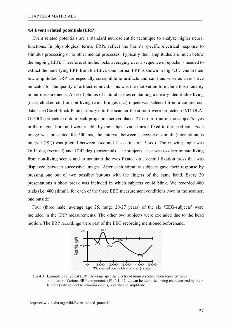
CHAPTER 4 MATERIALS
27
4.4 Event related potentials (ERP)
Event related potentials are a standard neuroscientific technique to analyze higher neural
functions. In physiological terms, ERPs reflect the brain’s specific electrical response to
stimulus processing or to other mental processes. Typically their amplitudes are much below
the ongoing EEG. Therefore, stimulus locks averaging over a sequence of epochs is needed to
extract the underlying ERP from the EEG. One normal ERP is shown in Fig.4.31. Due to their
low amplitudes ERP are especially susceptible to artifacts and can thus serve as a sensitive
indicator for the quality of artifact removal. This was the motivation to include this modality
in our measurements. A set of photos of natural scenes containing a clearly identifiable living
(deer, chicken etc.) or non-living (cars, bridges etc.) object was selected from a commercial
database (Corel Stock Photo Library). In the scanner the stimuli were projected (JVC DLA-
G150CL projector) onto a back-projection screen placed 27 cm in front of the subject’s eyes
in the magnet bore and were visible by the subject via a mirror fixed to the head coil. Each
image was presented for 500 ms, the interval between successive stimuli (inter stimulus
interval (ISI)) was jittered between 1sec and 2 sec (mean 1.5 sec). The viewing angle was
26.1° deg (vertical) and 17.4° deg (horizontal). The subjects’ task was to discriminate living
from non-living scenes and to maintain the eyes fixated on a central fixation cross that was
displayed between successive images. After each stimulus subjects gave their response by
pressing one out of two possible buttons with the fingers of the same hand. Every 20
presentations a short break was included in which subjects could blink. We recorded 480
trials (i.e. 480 stimuli) for each of the three EEG measurement conditions (two in the scanner,
one outside).
Four (three male, average age 25, range 20-27 years) of the six ‘EEG-subjects’ were
included in the ERP measurements. The other two subjects were excluded due to the head
motion. The ERP recordings were part of the EEG recording mentioned beforehand.
Fig.4.3 Example of a typical ERP1: Average specific electrical brain response upon repeated visual
stimulation. Various ERP components (P1, N1, P2,…) can be identified being characterized by their latency (with respect to stimulus onset), polarity and amplitude.
1 http://en.wikipedia.org/wiki/Event-related_potential
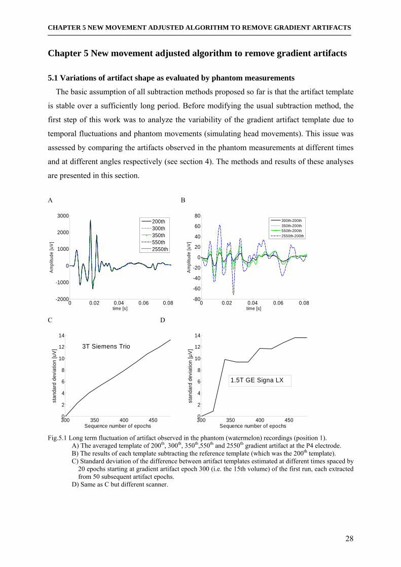
CHAPTER 5 NEW MOVEMENT ADJUSTED ALGORITHM TO REMOVE GRADIENT ARTIFACTS
28
Chapter 5 New movement adjusted algorithm to remove gradient artifacts 5.1 Variations of artifact shape as evaluated by phantom measurements
The basic assumption of all subtraction methods proposed so far is that the artifact template
is stable over a sufficiently long period. Before modifying the usual subtraction method, the
first step of this work was to analyze the variability of the gradient artifact template due to
temporal fluctuations and phantom movements (simulating head movements). This issue was
assessed by comparing the artifacts observed in the phantom measurements at different times
and at different angles respectively (see section 4). The methods and results of these analyses
are presented in this section.
A B
0 0.02 0.04 0.06 0.08-2000
-1000
0
1000
2000
3000
Am
plitu
de [u
V]
time [s]
200th300th350th550th2550th
0 0.02 0.04 0.06 0.08-80
-60
-40
-20
0
20
40
60
80
Am
plitu
de [u
V]
time [s]
300th-200th350th-200th550th-200th2550th-200th
C D
300 350 400 4500
2
4
6
8
10
12
14
Sequence number of epochs
stan
dard
dev
iatio
n [u
V]
3T Siemens Trio
300 350 400 4500
2
4
6
8
10
12
14
Sequence number of epochs
stan
dard
dev
iatio
n [µ
V]
1.5T GE Signa LX
Fig.5.1 Long term fluctuation of artifact observed in the phantom (watermelon) recordings (position 1).
A) The averaged template of 200th, 300th, 350th,550th and 2550th gradient artifact at the P4 electrode. B) The results of each template subtracting the reference template (which was the 200th template). C) Standard deviation of the difference between artifact templates estimated at different times spaced by
20 epochs starting at gradient artifact epoch 300 (i.e. the 15th volume) of the first run, each extracted from 50 subsequent artifact epochs.
D) Same as C but different scanner.
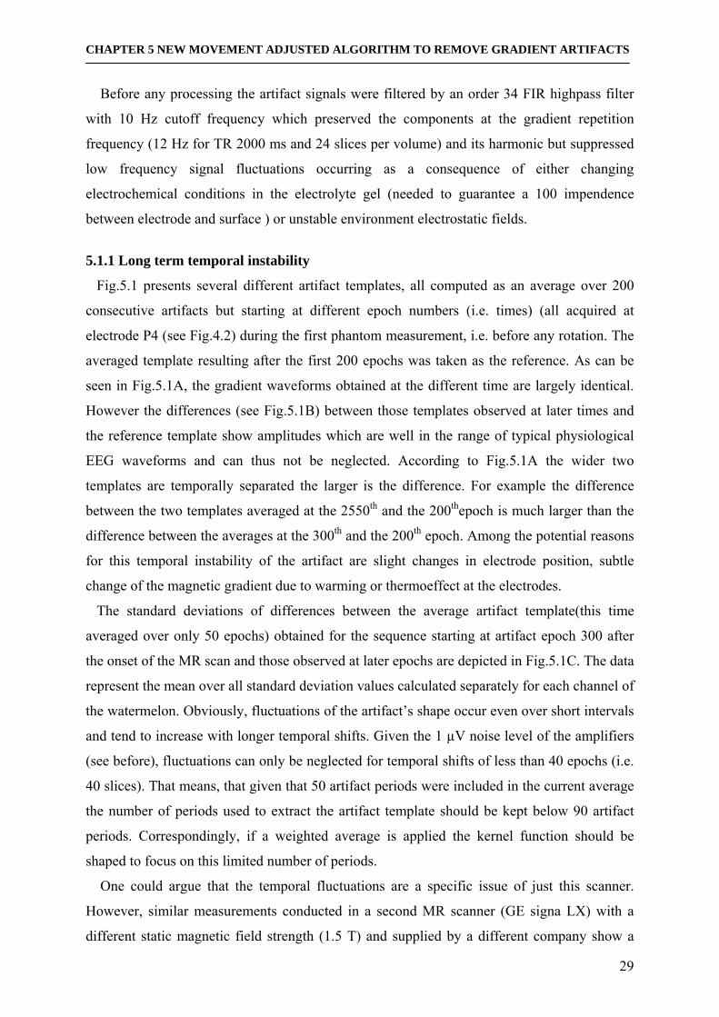
CHAPTER 5 NEW MOVEMENT ADJUSTED ALGORITHM TO REMOVE GRADIENT ARTIFACTS
29
Before any processing the artifact signals were filtered by an order 34 FIR highpass filter
with 10 Hz cutoff frequency which preserved the components at the gradient repetition
frequency (12 Hz for TR 2000 ms and 24 slices per volume) and its harmonic but suppressed
low frequency signal fluctuations occurring as a consequence of either changing
electrochemical conditions in the electrolyte gel (needed to guarantee a 100 impendence
between electrode and surface ) or unstable environment electrostatic fields.
5.1.1 Long term temporal instability
Fig.5.1 presents several different artifact templates, all computed as an average over 200
consecutive artifacts but starting at different epoch numbers (i.e. times) (all acquired at
electrode P4 (see Fig.4.2) during the first phantom measurement, i.e. before any rotation. The
averaged template resulting after the first 200 epochs was taken as the reference. As can be
seen in Fig.5.1A, the gradient waveforms obtained at the different time are largely identical.
However the differences (see Fig.5.1B) between those templates observed at later times and
the reference template show amplitudes which are well in the range of typical physiological
EEG waveforms and can thus not be neglected. According to Fig.5.1A the wider two
templates are temporally separated the larger is the difference. For example the difference
between the two templates averaged at the 2550th and the 200thepoch is much larger than the
difference between the averages at the 300th and the 200th epoch. Among the potential reasons
for this temporal instability of the artifact are slight changes in electrode position, subtle
change of the magnetic gradient due to warming or thermoeffect at the electrodes.
The standard deviations of differences between the average artifact template(this time
averaged over only 50 epochs) obtained for the sequence starting at artifact epoch 300 after
the onset of the MR scan and those observed at later epochs are depicted in Fig.5.1C. The data
represent the mean over all standard deviation values calculated separately for each channel of
the watermelon. Obviously, fluctuations of the artifact’s shape occur even over short intervals
and tend to increase with longer temporal shifts. Given the 1 µV noise level of the amplifiers
(see before), fluctuations can only be neglected for temporal shifts of less than 40 epochs (i.e.
40 slices). That means, that given that 50 artifact periods were included in the current average
the number of periods used to extract the artifact template should be kept below 90 artifact
periods. Correspondingly, if a weighted average is applied the kernel function should be
shaped to focus on this limited number of periods.
One could argue that the temporal fluctuations are a specific issue of just this scanner.
However, similar measurements conducted in a second MR scanner (GE signa LX) with a
different static magnetic field strength (1.5 T) and supplied by a different company show a
CHAPTER 5 NEW MOVEMENT ADJUSTED ALGORITHM TO REMOVE GRADIENT ARTIFACTS
30
very much comparable variability of the gradient artifact waveform (see Fig.5.1D) thus
suggesting that this observation reflects a more general effect.
5.1.2 Variability depending on MR-slice
Besides long term variation, the gradient artifacts may also differ in shape depending on the
slice number within each volume. To evaluate this potential source of variability, a slice-
based averaged method was applied to create slice-specific templates by averaging only over
those epochs obtained at the same slice number within the different volumes (i.e., the 1st slice-
number template is averaged over all 1st slices in each volume). Fig.5.2 shows the fluctuations
of the standard deviations of the subtracted resulting differences between all but the first slice-
based templates and the first slice-based template (each slice template averaged over all
volumes). These results clearly show that the between slices differences of the gradient
artifact are negligible given the amplifier noise level of about 1 µV STD. Obviously, the long
term variability by far exceeds the slice-dependent variation.
2 4 6 8 10 12 14 16 18 20 22 240.75
0.8
0.85
0.9
0.95
1
1.05
1.1
1.15
slice number within a volume [n]
stan
dard
dev
iatio
n [u
V]
Fig.5.2 Test of slice-specific averaged template conducted with the data recorded with the phantom (watermelon, position 1, electrode Cz): The std of difference between all but the first and the first slice in one volume. The alignments between all epochs used to generate the slice-specific templates were assembled applying the resampling technique (see section 5.3.4.3). 5.1.3 Variations due to electrode movements
Next, unavoidable head movements were analysed as potential sources of artifact template
variations. For this purpose we recorded phantom EEG signal at four different phantom
orientations (See Fig.4.2) in order to measure the influence of the electrode positions on the
template. During this experiment, the phantom was rotated by a fixed angle increment
between consecutive recordings. During each recording its position was fixed by a hard
plastic block as shown in Fig.4.2. The rotated watermelon simulates the head motion of the
subject along y-direction. Regarding electrode P4 (See Fig.4.2) which was evaluated here, the
displacement per rotation step was about 0.5 mm in the vertical (i.e. y) direction resulting
from a 2.4 mm displacement in tangential direction which is comparable to a realistic strong

CHAPTER 5 NEW MOVEMENT ADJUSTED ALGORITHM TO REMOVE GRADIENT ARTIFACTS
31
head movement. A representative template for each position was derived by averaging over
200 consecutive gradient artifacts waveforms. The resulting templates are shown in Fig.5.3
for the four different phantom positions. Although the phantom was rotated by a slight degree,
the electrodes may be rotated with a different degree (more or less). Therefore, the different
channel shows the different changes for the four positions in Fig.5.3A and 5.3B. Obviously, at
these slight rotations the artifact templates significantly change their shape giving rise to the
idea of including head movement information in the algorithm to extract the subtracted
template. A B
0 0.02 0.04 0.06 0.08-5000-4000-3000-2000-1000
010002000300040005000
Am
plitu
de [u
V]
Time [s]
Channel P4
position 1position 2position 3position 4
0 0.02 0.04 0.06 0.08-4000
-2000
0
2000
4000
6000A
mpl
itude
[uV
]
Time [s]
Channel P7
position 1position 2position 3position 4
Fig.5.3 Artifact waveform as recorded in the phantom (watermelon) recordings in four different positions.
Each separated by a rotation of 2 degrees, keeping the absolute position within the MR bore. A) The pattern at the P4 electrode (see Fig. 4.2) B) The pattern at the P7 electrode
5.2 Deriving a head movements indicator
It is impossible for subjects to stay motionless during the whole scanning period. Having in
mind the motion-dependence of the artifact shape, it is necessary to design an additional
system to track the head motion as a premise for a motion guided artifact removal concept.
This system will help us locate the relative position of electrodes accurately and subsequently
classify and average the gradient artifacts according to electrodes position in order to achieve
the least error of the residual gradient artifacts. An eye tracker system (Kanowski et al., 2007)
can be modified to serve as such a tool (see section 5.2.2 (below) for details) but it needs
some extra hardware parts which usually not available in MR laboratories. Another method,
using the alignment function of the freely available statistical parametric mapping (SPM)
software package can replace the procedure of the hardware movement tracking.
SPM was developed by the Functional Imaging Lab (FIL) London for (i) image
preprocessing and (ii) statistical analysis in the context of functional imaging (either fMRI or
positron emission tomography (PET)). In the case of fMRI analysis the sequence of BOLD
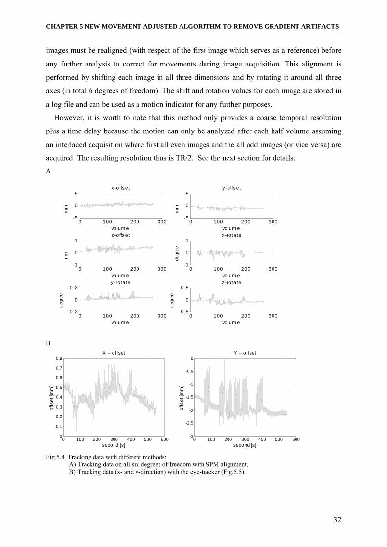
CHAPTER 5 NEW MOVEMENT ADJUSTED ALGORITHM TO REMOVE GRADIENT ARTIFACTS
32
images must be realigned (with respect of the first image which serves as a reference) before
any further analysis to correct for movements during image acquisition. This alignment is
performed by shifting each image in all three dimensions and by rotating it around all three
axes (in total 6 degrees of freedom). The shift and rotation values for each image are stored in
a log file and can be used as a motion indicator for any further purposes.
However, it is worth to note that this method only provides a coarse temporal resolution
plus a time delay because the motion can only be analyzed after each half volume assuming
an interlaced acquisition where first all even images and the all odd images (or vice versa) are
acquired. The resulting resolution thus is TR/2. See the next section for details. A
0 100 200 300-5
0
5
volum e
mm
x -offs et
0 100 200 300-5
0
5
volum e
mm
y -offs et
0 100 200 300-1
0
1
volum e
mm
z -offs et
0 100 200 300-1
0
1
volum e
degr
ee
x -rotate
0 100 200 300-0.2
0
0.2
volum e
degr
ee
y -rotate
0 100 200 300-0.5
0
0.5
volum e
degr
ee
z -rotate
B
0 100 200 300 400 500 6000
0.1
0.2
0.3
0.4
0.5
0.6
0.7
0.8X -- offset
second [s]
offs
et [m
m]
0 100 200 300 400 500 600-3
-2.5
-2
-1.5
-1
-0.5
0Y -- offset
second [s]
offs
et [m
m]
Fig.5.4 Tracking data with different methods:
A) Tracking data on all six degrees of freedom with SPM alignment. B) Tracking data (x- and y-direction) with the eye-tracker (Fig.5.5).
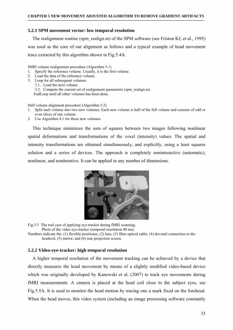
CHAPTER 5 NEW MOVEMENT ADJUSTED ALGORITHM TO REMOVE GRADIENT ARTIFACTS
33
5.2.1 SPM movement vector: low temporal resolution
The realignment routine (spm_realign.m) of the SPM software (see Friston KJ, et al., 1995)
was used as the core of our alignment as follows and a typical example of head movement
trace extracted by this algorithm shown in Fig.5.4A. fMRI volume realignment procedure (Algorithm 5.1) 1. Specify the reference volume. Usually, it is the first volume. 2. Load the data of the reference volume. 3. Loop for all subsequent volumes
3.1. Load the next volume. 3.2. Compute the current set of realignment parameters (spm_realign.m).
EndLoop until all other volumes has been done.
Half volume alignment procedure (Algorithm 5.2) 1. Split each volume into two new volumes. Each new volume is half of the full volume and consists of odd or
even slices of one volume. 2. Use Algorithm 4.1 for these new volumes. This technique minimizes the sum of squares between two images following nonlinear
spatial deformations and transformations of the voxel (intensity) values. The spatial and
intensity transformations are obtained simultaneously, and explicitly, using a least squares
solution and a series of devices. The approach is completely noninteractive (automatic),
nonlinear, and noniterative. It can be applied in any number of dimensions.
Fig.5.5 The real case of applying eye-tracker during fMRI scanning.
Photo of the video eye-tracker (temporal resolution 40 ms). Numbers indicate the: (1) flexible positioner, (2) lens, (3) fibre optical cable, (4) dovetail connection to the
headcoil, (5) mirror, and (6) rear projection screen.
5.2.2 Video-eye-tracker: high temporal resolution
A higher temporal resolution of the movement tracking can be achieved by a device that
directly measures the head movement by means of a slightly modified video-based device
which was originally developed by Kanowski et al. (2007) to track eye movements during
fMRI measurements. A camera is placed at the head coil close to the subject eyes, see
Fig.5.5A. It is used to monitor the head motion by tracing one a mark fixed on the forehead.
When the head moves, this video system (including an image processing software constantly
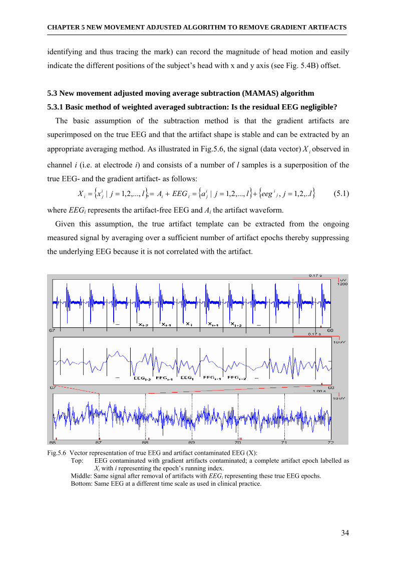
CHAPTER 5 NEW MOVEMENT ADJUSTED ALGORITHM TO REMOVE GRADIENT ARTIFACTS
34
identifying and thus tracing the mark) can record the magnitude of head motion and easily
indicate the different positions of the subject’s head with x and y axis (see Fig. 5.4B) offset.
5.3 New movement adjusted moving average subtraction (MAMAS) algorithm
5.3.1 Basic method of weighted averaged subtraction: Is the residual EEG negligible?
The basic assumption of the subtraction method is that the gradient artifacts are
superimposed on the true EEG and that the artifact shape is stable and can be extracted by an
appropriate averaging method. As illustrated in Fig.5.6, the signal (data vector) iX observed in
channel i (i.e. at electrode i) and consists of a number of l samples is a superposition of the
true EEG- and the gradient artifact- as follows:
ljeegljaEEGAljxX jii
jiiiji ,..2,1,,...,2,1|,,...,2,1| =+==+=== (5.1)
where EEGi represents the artifact-free EEG and Ai the artifact waveform.
Given this assumption, the true artifact template can be extracted from the ongoing
measured signal by averaging over a sufficient number of artifact epochs thereby suppressing
the underlying EEG because it is not correlated with the artifact.
Fig.5.6 Vector representation of true EEG and artifact contaminated EEG (X):
Top: EEG contaminated with gradient artifacts contaminated; a complete artifact epoch labelled as Xi with i representing the epoch’s running index.
Middle: Same signal after removal of artifacts with EEGi representing these true EEG epochs. Bottom: Same EEG at a different time scale as used in clinical practice.
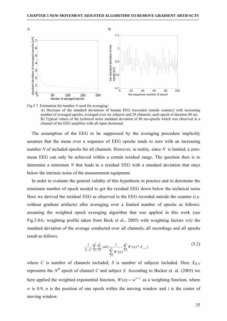
CHAPTER 5 NEW MOVEMENT ADJUSTED ALGORITHM TO REMOVE GRADIENT ARTIFACTS
35
A B
0 50 100 150 2000
1
2
3
4
5
6
7
Number of averaged epochs
stan
dard
dev
iatio
n of
ave
rage
d ep
ochs
[uV
]
Fig.5.7 Estimation the number N used for averaging:
A) Decrease of the standard deviations of human EEG (recorded outside scanner) with increasing number of averaged epochs, averaged over six subjects and 29 channels; each epoch of duration 80 ms. B) Typical values of the technical noise standard deviation of 80 ms-epochs which was observed in a channel of the EEG amplifier with all input shortened.
The assumption of the EEG to be suppressed by the averaging procedure implicitly
assumes that the mean over a sequence of EEG epochs tends to zero with an increasing
number N of included epochs for all channels. However, in reality, since N is limited, a zero-
mean EEG can only be achieved within a certain residual range. The question then is to
determine a minimum N that leads to a residual EEG with a standard deviation that stays
below the intrinsic noise of the measurement equipment.
In order to evaluate the general validity of this hypothesis in practice and to determine the
minimum number of epoch needed to get the residual EEG down below the technical noise
floor we derived the residual EEG as observed in the EEG recorded outside the scanner (i.e.
without gradient artifacts) after averaging over a limited number of epochs as follows:
assuming the weighted epoch averaging algorithm that was applied in this work (see
Fig.5.8A; weighting profile taken from Beck et al., 2005) with weighting factors w(i) the
standard deviation of the average conducted over all channels, all recordings and all epochs
result as follows.
∑∑ ∑∑= = =
=
⋅
S
s
C
c
N
nscnN
n
XnWnW
stdCS 1 1 1
1
)*)()(
1(1
(5.2)
where C is number of channels included, S is number of subjects included. Here XSCN
represents the Nth epoch of channel C and subject S. According to Becker et. al. (2005) we
here applied the weighted exponential function, inwnW −=)( as a weighting function, where
w is 0.9, n is the position of one epoch within the moving window and i is the center of
moving window.
0 20 40 60 80 100 0.7
0.8
0.9
1
1.1
the sequence number of epoch
the
stan
dard
dev
iatio
n of
the
epoc
h [u
V]
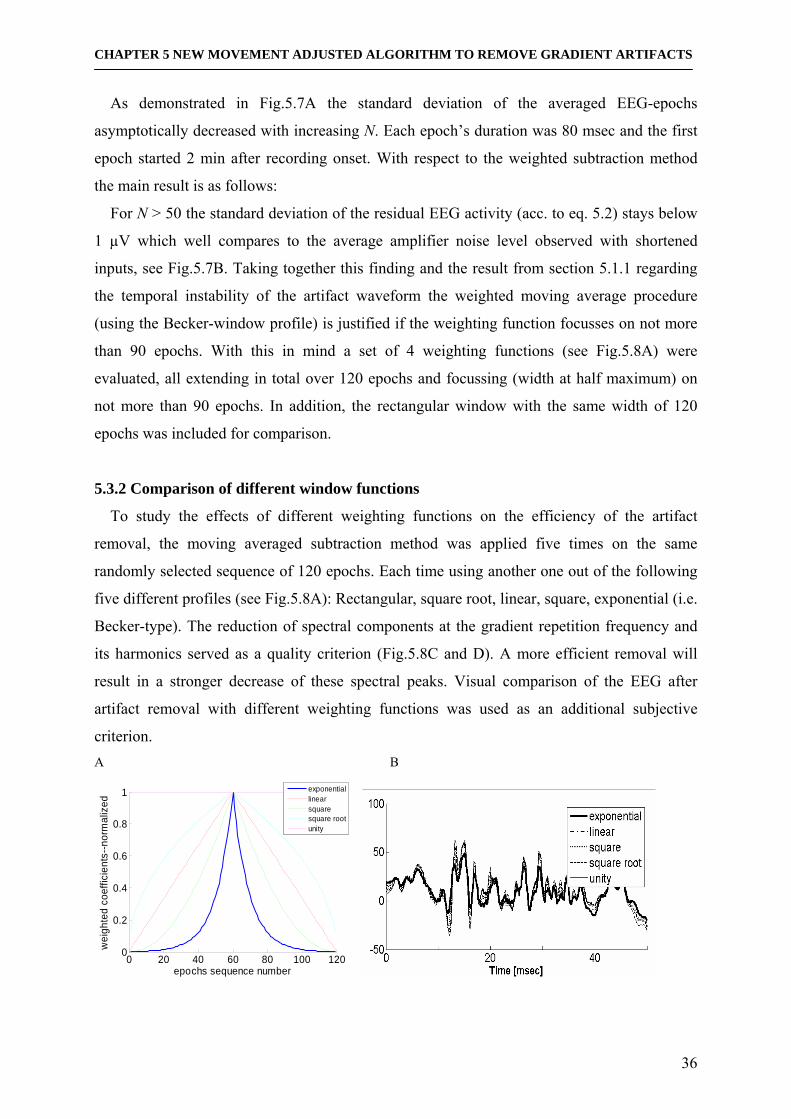
CHAPTER 5 NEW MOVEMENT ADJUSTED ALGORITHM TO REMOVE GRADIENT ARTIFACTS
36
As demonstrated in Fig.5.7A the standard deviation of the averaged EEG-epochs
asymptotically decreased with increasing N. Each epoch’s duration was 80 msec and the first
epoch started 2 min after recording onset. With respect to the weighted subtraction method
the main result is as follows:
For N > 50 the standard deviation of the residual EEG activity (acc. to eq. 5.2) stays below
1 µV which well compares to the average amplifier noise level observed with shortened
inputs, see Fig.5.7B. Taking together this finding and the result from section 5.1.1 regarding
the temporal instability of the artifact waveform the weighted moving average procedure
(using the Becker-window profile) is justified if the weighting function focusses on not more
than 90 epochs. With this in mind a set of 4 weighting functions (see Fig.5.8A) were
evaluated, all extending in total over 120 epochs and focussing (width at half maximum) on
not more than 90 epochs. In addition, the rectangular window with the same width of 120
epochs was included for comparison.
5.3.2 Comparison of different window functions
To study the effects of different weighting functions on the efficiency of the artifact
removal, the moving averaged subtraction method was applied five times on the same
randomly selected sequence of 120 epochs. Each time using another one out of the following
five different profiles (see Fig.5.8A): Rectangular, square root, linear, square, exponential (i.e.
Becker-type). The reduction of spectral components at the gradient repetition frequency and
its harmonics served as a quality criterion (Fig.5.8C and D). A more efficient removal will
result in a stronger decrease of these spectral peaks. Visual comparison of the EEG after
artifact removal with different weighting functions was used as an additional subjective
criterion. A B
0 20 40 60 80 100 1200
0.2
0.4
0.6
0.8
1
epochs sequence number
wei
ghte
d co
effic
ient
s--n
orm
aliz
ed
exponentiallinearsquaresquare rootunity
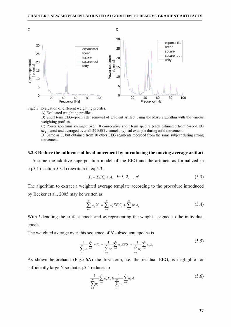
CHAPTER 5 NEW MOVEMENT ADJUSTED ALGORITHM TO REMOVE GRADIENT ARTIFACTS
37
C D
20 40 60 80 1000
5
10
15
20
25
30
Frequency [Hz]
Pow
er s
pect
rum
[re
l.uni
ts]
exponentiallinearsquaresquare rootunity
20 40 60 80 1000
5
10
15
20
25
30
Frequency [Hz]
Pow
er s
pect
rum
[rel.
units
]
exponentiallinearsquaresquare rootunity
Fig.5.8 Evaluation of different weighting profiles.
A) Evaluated weighting profiles. B) Short term EEG-epoch after removal of gradient artifact using the MAS algorithm with the various weighting profiles. C) Power spectrum averaged over 10 consecutive short term spectra (each estimated from 6-sec-EEG segments) and averaged over all 29 EEG channels; typical example during mild movement. D) Same as C, but obtained from 10 other EEG segments recorded from the same subject during strong movement.
5.3.3 Reduce the influence of head movement by introducing the moving average artifact
Assume the additive superposition model of the EEG and the artifacts as formalized in
eq.5.1 (section 5.3.1) rewritten in eq.5.3.
iii AEEGX += , i=1, 2,…, N. (5.3)
The algorithm to extract a weighted average template according to the procedure introduced
by Becker et al., 2005 may be written as
∑∑∑===
+=N
iii
N
iii
N
iii AwEEGwXw
111 (5.4)
With i denoting the artifact epoch and wi representing the weight assigned to the individual
epoch.
The weighted average over this sequence of N subsequent epochs is
∑∑
∑∑
∑∑ =
=
=
=
=
=
+=N
iiiN
ii
N
iiiN
ii
N
iiiN
ii
Aww
EEGww
Xww 1
1
1
1
1
1
111 (5.5)
As shown beforehand (Fig.5.6A) the first term, i.e. the residual EEG, is negligible for
sufficiently large N so that eq.5.5 reduces to
∑∑
∑∑ =
=
=
=
≅N
iiiN
ii
N
iiiN
ii
Aww
Xww 1
1
1
1
11 (5.6)
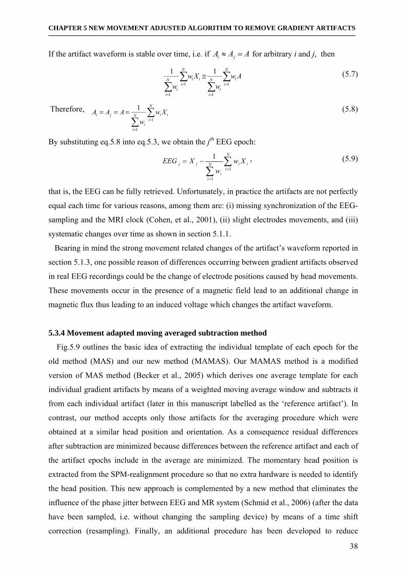
CHAPTER 5 NEW MOVEMENT ADJUSTED ALGORITHM TO REMOVE GRADIENT ARTIFACTS
38
If the artifact waveform is stable over time, i.e. if AAA ji =≈ for arbitrary i and j, then
Aww
Xww
N
iiN
ii
N
iiiN
ii
∑∑
∑∑ =
=
=
=
≅1
1
1
1
11 (5.7)
Therefore, ∑∑ =
=
===N
iiiN
ii
ji Xww
AAA1
1
1
(5.8)
By substituting eq.5.8 into eq.5.3, we obtain the jth EEG epoch:
∑∑ =
=
−=N
iiiN
ii
jj Xww
XEEG1
1
1 , (5.9)
that is, the EEG can be fully retrieved. Unfortunately, in practice the artifacts are not perfectly
equal each time for various reasons, among them are: (i) missing synchronization of the EEG-
sampling and the MRI clock (Cohen, et al., 2001), (ii) slight electrodes movements, and (iii)
systematic changes over time as shown in section 5.1.1.
Bearing in mind the strong movement related changes of the artifact’s waveform reported in
section 5.1.3, one possible reason of differences occurring between gradient artifacts observed
in real EEG recordings could be the change of electrode positions caused by head movements.
These movements occur in the presence of a magnetic field lead to an additional change in
magnetic flux thus leading to an induced voltage which changes the artifact waveform.
5.3.4 Movement adapted moving averaged subtraction method
Fig.5.9 outlines the basic idea of extracting the individual template of each epoch for the
old method (MAS) and our new method (MAMAS). Our MAMAS method is a modified
version of MAS method (Becker et al., 2005) which derives one average template for each
individual gradient artifacts by means of a weighted moving average window and subtracts it
from each individual artifact (later in this manuscript labelled as the ‘reference artifact’). In
contrast, our method accepts only those artifacts for the averaging procedure which were
obtained at a similar head position and orientation. As a consequence residual differences
after subtraction are minimized because differences between the reference artifact and each of
the artifact epochs include in the average are minimized. The momentary head position is
extracted from the SPM-realignment procedure so that no extra hardware is needed to identify
the head position. This new approach is complemented by a new method that eliminates the
influence of the phase jitter between EEG and MR system (Schmid et al., 2006) (after the data
have been sampled, i.e. without changing the sampling device) by means of a time shift
correction (resampling). Finally, an additional procedure has been developed to reduce

CHAPTER 5 NEW MOVEMENT ADJUSTED ALGORITHM TO REMOVE GRADIENT ARTIFACTS
39
residual artifacts remaining in case of brief fast movements (not adequately detected by the
SPM with its temporal resolution of 1 sec) after the MAMAS procedure. The outline of this
method is described in algorithm 5.3.
EEG
HeadMotionMonitor data
Old New
+ +
... ... ... ...
The current artifact
∑=
N
jjw
0
wi Wi+1 Wi+2 Wi+3Wi-1Wi-2Wi-3wi Wi+1 Wi+2 Wi+3Wi-1Wi-5Wi-4 Wi-3Wi-2Wi-6Wi-7Wi-8 ÷÷
÷ ∑=
N
jjw
0÷
Fig.5.9 Schematic diagram of MAS(old) and MAMAS(new) GAR removal methods
MAMAS (Algorithm 5.3) 1. Detect onsets of gradient artifacts. 2. Class gradient artifacts into different levels guided by SPM-head motion monitoring data. 3. Create for each individual gradient an individual average artifact template by averaging over epochs
obtained at the same head position levels. The resampling technique is applied to each epoch. 4. Subtract the individual template from the corresponding gradient artifact. 5. Detect residual gradient artifacts occurring in case of brief motion. 6. Apply the special algorithm to reduce this residual artifact. 5.3.4.1 Detection of gradient artifact onsets
The number of samples (l ) per artifact epoch can be directly determined from the MR-
repetition time (TR), the number of slices per volume (nsl) and the EEG sampling frequency
(fs) according to the following rule:
fsnslTRl ⋅= (5.10)
With this number one could in principle predict the onsets of all artifact epochs once the start
of the first epoch has been determined. However, in practice this leads to inaccuracies since
the TR value is only known with limited precision leading to a shift of several samples
between theoretical and effective onsets of the artifact epochs (see also Goncalves et al.
(2007a) for further discussion of this issue). In addition, as already described in section 3.1,
the missing synchronization between the EEG sampling clock and the MR-timer causes an
CHAPTER 5 NEW MOVEMENT ADJUSTED ALGORITHM TO REMOVE GRADIENT ARTIFACTS
40
additional alignment error (‘phase jitter’). As a consequence the onsets of the artifact epochs
need to be determined before any further processing.
The purpose of the first part of this algorithm (described in the current section) is the
alignment of the artifacts keeping an accuracy of on sampling whereas the adjustment of
asynchronous clock errors will be addressed in the over next section 5.3.3 introducing a new
resampling technique.
A B
0 0.02 0.04 0.06 0.08 0.1
-6000
-4000
-2000
0
2000
4000
ampl
itude
(uV
)
time(s)0 0.02 0.04 0.06 0.08 0.1
-6000
-4000
-2000
0
2000
4000
ampl
itude
(uV
)
time(s) C
Fig.5.10 Adjustment of the gradient artifact onsets with respect to the MRI triggers: (subject km42).
A) Overlay of 50 gradient artifacts according to the MRI triggers. B) Adjustment these onsets with algorithm 5.4. C) Variance observed at different shift intervals.
In the following two alternative methods will be described to determine and adjust the
artifact epochs. The first method uses a trigger signal provided by the MRI to indicate the
acquisition of the next slice. If this MRI trigger is available (which is the case in the scanner
used here), the gradient artifact onset can be retrieved directly using the markers recorded
simultaneously with the EEG. However, an additional realignment algorithm is needed to
cope with the fact that in practice a tiny jitter occurs between the effective onset of the artifact
and the trigger (see Fig.5.10A). For this purpose the onsets are adjusted by calculating the
variance of the difference between the reference artifact, usually the first one, and all other
-40 -30 -20 -10 0 100
2
4
6
8
10 x 10 7
Vara
nce
of th
e di
ffere
nce
[uV2 ]
offset points number:left shift is negative number, right shift is positive number
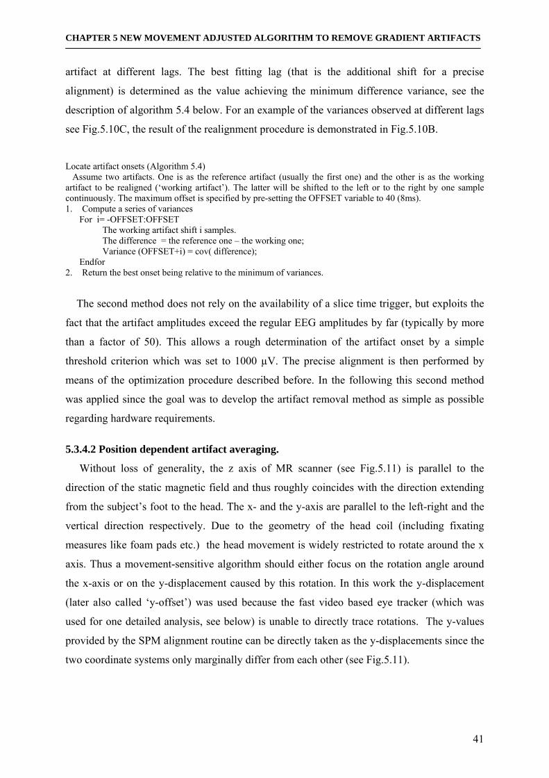
CHAPTER 5 NEW MOVEMENT ADJUSTED ALGORITHM TO REMOVE GRADIENT ARTIFACTS
41
artifact at different lags. The best fitting lag (that is the additional shift for a precise
alignment) is determined as the value achieving the minimum difference variance, see the
description of algorithm 5.4 below. For an example of the variances observed at different lags
see Fig.5.10C, the result of the realignment procedure is demonstrated in Fig.5.10B.
Locate artifact onsets (Algorithm 5.4) Assume two artifacts. One is as the reference artifact (usually the first one) and the other is as the working artifact to be realigned (‘working artifact’). The latter will be shifted to the left or to the right by one sample continuously. The maximum offset is specified by pre-setting the OFFSET variable to 40 (8ms). 1. Compute a series of variances For i= -OFFSET:OFFSET The working artifact shift i samples. The difference = the reference one – the working one; Variance (OFFSET+i) = cov( difference); Endfor 2. Return the best onset being relative to the minimum of variances.
The second method does not rely on the availability of a slice time trigger, but exploits the
fact that the artifact amplitudes exceed the regular EEG amplitudes by far (typically by more
than a factor of 50). This allows a rough determination of the artifact onset by a simple
threshold criterion which was set to 1000 µV. The precise alignment is then performed by
means of the optimization procedure described before. In the following this second method
was applied since the goal was to develop the artifact removal method as simple as possible
regarding hardware requirements.
5.3.4.2 Position dependent artifact averaging.
Without loss of generality, the z axis of MR scanner (see Fig.5.11) is parallel to the
direction of the static magnetic field and thus roughly coincides with the direction extending
from the subject’s foot to the head. The x- and the y-axis are parallel to the left-right and the
vertical direction respectively. Due to the geometry of the head coil (including fixating
measures like foam pads etc.) the head movement is widely restricted to rotate around the x
axis. Thus a movement-sensitive algorithm should either focus on the rotation angle around
the x-axis or on the y-displacement caused by this rotation. In this work the y-displacement
(later also called ‘y-offset’) was used because the fast video based eye tracker (which was
used for one detailed analysis, see below) is unable to directly trace rotations. The y-values
provided by the SPM alignment routine can be directly taken as the y-displacements since the
two coordinate systems only marginally differ from each other (see Fig.5.11).
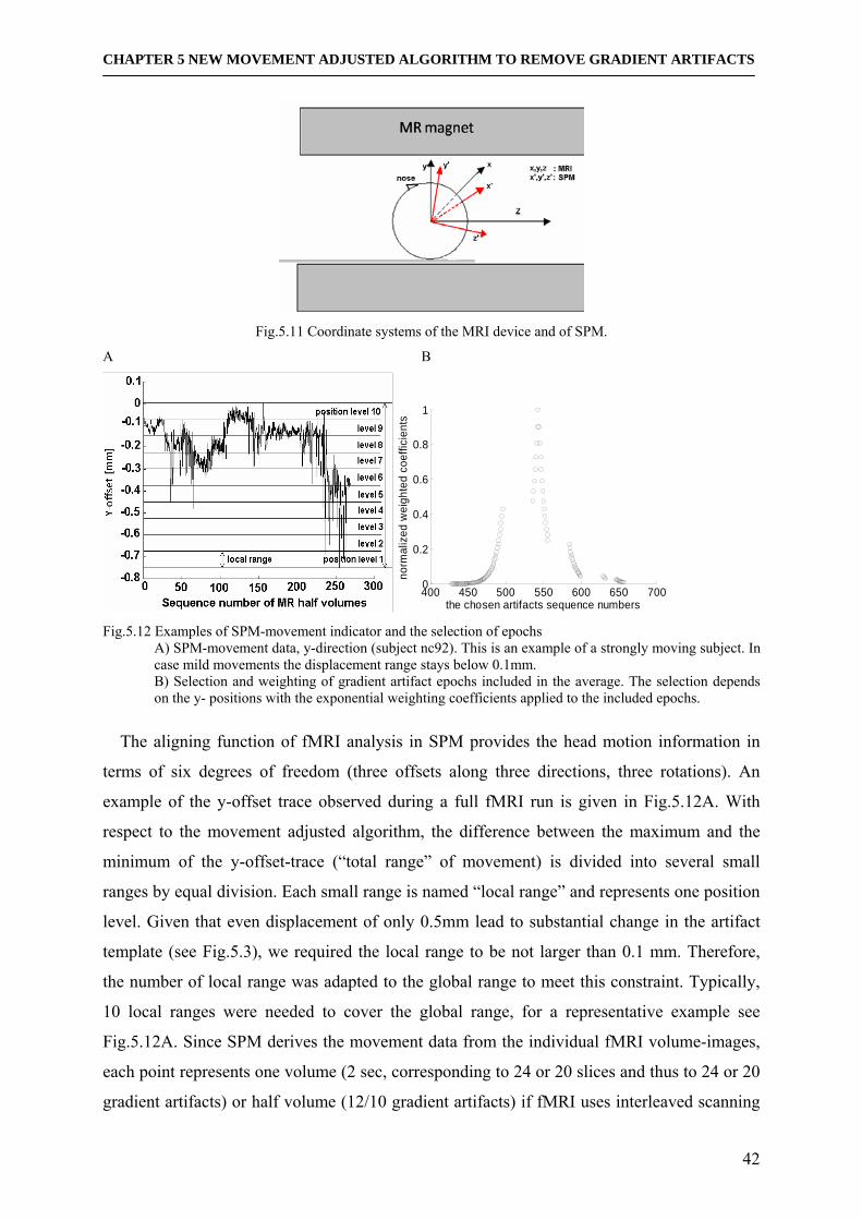
CHAPTER 5 NEW MOVEMENT ADJUSTED ALGORITHM TO REMOVE GRADIENT ARTIFACTS
42
Fig.5.11 Coordinate systems of the MRI device and of SPM.
A B
400 450 500 550 600 650 7000
0.2
0.4
0.6
0.8
1
the chosen artifacts sequence numbers
norm
aliz
ed w
eigh
ted
coef
ficie
nts
Fig.5.12 Examples of SPM-movement indicator and the selection of epochs
A) SPM-movement data, y-direction (subject nc92). This is an example of a strongly moving subject. In case mild movements the displacement range stays below 0.1mm. B) Selection and weighting of gradient artifact epochs included in the average. The selection depends on the y- positions with the exponential weighting coefficients applied to the included epochs.
The aligning function of fMRI analysis in SPM provides the head motion information in
terms of six degrees of freedom (three offsets along three directions, three rotations). An
example of the y-offset trace observed during a full fMRI run is given in Fig.5.12A. With
respect to the movement adjusted algorithm, the difference between the maximum and the
minimum of the y-offset-trace (“total range” of movement) is divided into several small
ranges by equal division. Each small range is named “local range” and represents one position
level. Given that even displacement of only 0.5mm lead to substantial change in the artifact
template (see Fig.5.3), we required the local range to be not larger than 0.1 mm. Therefore,
the number of local range was adapted to the global range to meet this constraint. Typically,
10 local ranges were needed to cover the global range, for a representative example see
Fig.5.12A. Since SPM derives the movement data from the individual fMRI volume-images,
each point represents one volume (2 sec, corresponding to 24 or 20 slices and thus to 24 or 20
gradient artifacts) or half volume (12/10 gradient artifacts) if fMRI uses interleaved scanning
CHAPTER 5 NEW MOVEMENT ADJUSTED ALGORITHM TO REMOVE GRADIENT ARTIFACTS
43
splitting the volume into two half volumes (corresponding to all even and odd numbered
slices) before aligning. This low sampling rate is adapted (i.e. upsampled) to the gradient
repetition rate by cubic spline interpolation. Next all gradient artifacts are classified into one
of the appropriate local range according to their y-offset. When the number of artifacts in one
level is below 200, the actual level is combined with the next larger or lower one to build a
new local range. This action transforms the uniform division into a non uniform distribution
of the local range width. This case often occurs at the fringe of the global range because the
number of epochs observed at the maximum and minimum local ranges is usually by far not
sufficient for the averaging procedure. Finally, the moving average window includes only
those artifacts which pertain to the same local range as the artifact to be removed.
When classification into levels is finished, the averaging procedure to generate a template
must obey the following three conditions. (i) The number of artifacts should be at least 50 in
order to keep the residual EEG below noise. (ii) The included artifacts should be temporally
located close to the current individual artifact to be removed by subtraction. The maximum
accepted distance is 200 epochs. (iii) If at least 50 epochs pertaining to the same local range
as the reference artifact is available within the 400 epoch-interval, then those at least 50
epochs (up to 120) are averaged applying the Becker weighting profile. However, if there are
less than 50 within local range of the reference artifact, epochs pertaining to adjacent local
ranges are accepted as well still applying the weighting function as shown in Fig.5.12B.
Schematic description of the selection algorithm (Algorithm 5.5) 1. Place the moving window (width is wd) such that the center of this window is the current – to be removed -
artifact and the current levels(l1 level and l2 level, l1 =l2) are the level of the current artifact. 2. Find artifacts which are in current levels (local ranges) in that window. 3. If a artifacts have been found, go to 7. 4. If the width of the current window is four times of the original one, go to 6. Otherwise go to 5. 5. If less than a artifacts have been found in the current window, then the width of the window is extended to
4*wd, go to 2. 6. If the width of the window has been extended to four times of the original width and the number of artifacts
is less than a, then set l1 = l1 - 1 and l2 =l2 + 1, reset the width of window to a, go to 2. 7. end
5.3.4.3 New resampling procedure to align sampling time of averaged artifact template
Given the large amplitude and its steep gradients of the artifacts under consideration, a
missing synchronization between the EEG sampling clock and the timing of the gradient
switching can lead to substantial residual artifacts after subtraction, unless each artifact
included in the average is resampled to match precisely the phase of the sampling points of
the artifact to be removed (‘reference artifact’). Resampling here means the calculation of
data samples at a predefined shifted grid of virtual sampling times. It has been proposed that
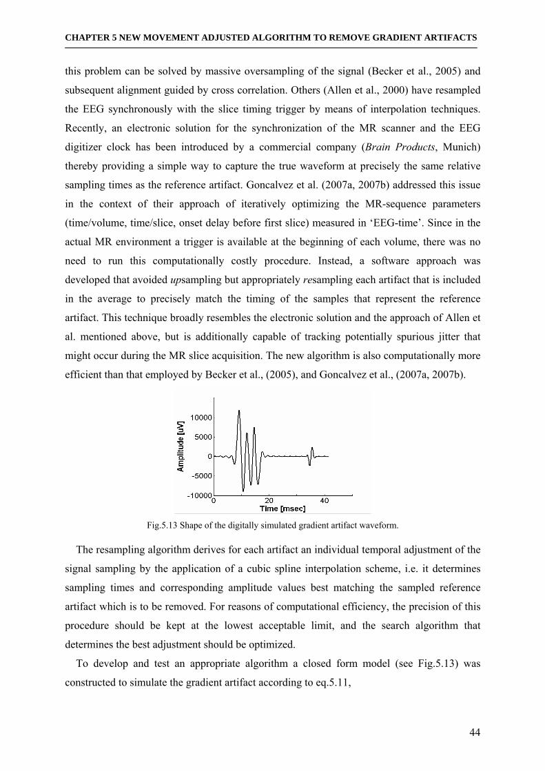
CHAPTER 5 NEW MOVEMENT ADJUSTED ALGORITHM TO REMOVE GRADIENT ARTIFACTS
44
this problem can be solved by massive oversampling of the signal (Becker et al., 2005) and
subsequent alignment guided by cross correlation. Others (Allen et al., 2000) have resampled
the EEG synchronously with the slice timing trigger by means of interpolation techniques.
Recently, an electronic solution for the synchronization of the MR scanner and the EEG
digitizer clock has been introduced by a commercial company (Brain Products, Munich)
thereby providing a simple way to capture the true waveform at precisely the same relative
sampling times as the reference artifact. Goncalvez et al. (2007a, 2007b) addressed this issue
in the context of their approach of iteratively optimizing the MR-sequence parameters
(time/volume, time/slice, onset delay before first slice) measured in ‘EEG-time’. Since in the
actual MR environment a trigger is available at the beginning of each volume, there was no
need to run this computationally costly procedure. Instead, a software approach was
developed that avoided upsampling but appropriately resampling each artifact that is included
in the average to precisely match the timing of the samples that represent the reference
artifact. This technique broadly resembles the electronic solution and the approach of Allen et
al. mentioned above, but is additionally capable of tracking potentially spurious jitter that
might occur during the MR slice acquisition. The new algorithm is also computationally more
efficient than that employed by Becker et al., (2005), and Goncalvez et al., (2007a, 2007b).
Fig.5.13 Shape of the digitally simulated gradient artifact waveform.
The resampling algorithm derives for each artifact an individual temporal adjustment of the
signal sampling by the application of a cubic spline interpolation scheme, i.e. it determines
sampling times and corresponding amplitude values best matching the sampled reference
artifact which is to be removed. For reasons of computational efficiency, the precision of this
procedure should be kept at the lowest acceptable limit, and the search algorithm that
determines the best adjustment should be optimized.
To develop and test an appropriate algorithm a closed form model (see Fig.5.13) was
constructed to simulate the gradient artifact according to eq.5.11,
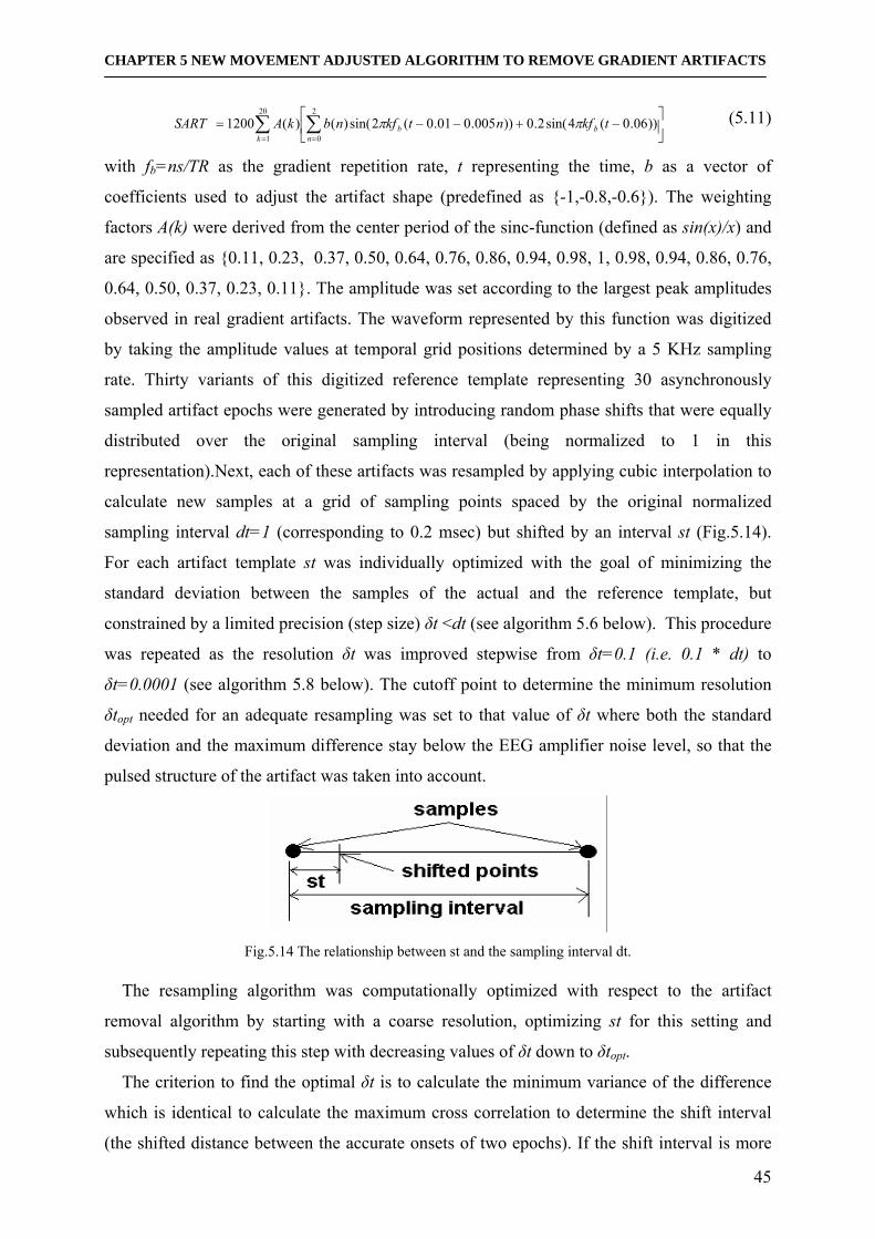
CHAPTER 5 NEW MOVEMENT ADJUSTED ALGORITHM TO REMOVE GRADIENT ARTIFACTS
45
∑ ∑= =
⎥⎦
⎤⎢⎣
⎡−+−−=
20
1
2
0))06.0(4sin(2.0))005.001.0(2sin()()(1200
kbb
ntkfntkfnbkASART ππ (5.11)
with fb=ns/TR as the gradient repetition rate, t representing the time, b as a vector of
coefficients used to adjust the artifact shape (predefined as -1,-0.8,-0.6). The weighting
factors A(k) were derived from the center period of the sinc-function (defined as sin(x)/x) and
are specified as 0.11, 0.23, 0.37, 0.50, 0.64, 0.76, 0.86, 0.94, 0.98, 1, 0.98, 0.94, 0.86, 0.76,
0.64, 0.50, 0.37, 0.23, 0.11. The amplitude was set according to the largest peak amplitudes
observed in real gradient artifacts. The waveform represented by this function was digitized
by taking the amplitude values at temporal grid positions determined by a 5 KHz sampling
rate. Thirty variants of this digitized reference template representing 30 asynchronously
sampled artifact epochs were generated by introducing random phase shifts that were equally
distributed over the original sampling interval (being normalized to 1 in this
representation).Next, each of these artifacts was resampled by applying cubic interpolation to
calculate new samples at a grid of sampling points spaced by the original normalized
sampling interval dt=1 (corresponding to 0.2 msec) but shifted by an interval st (Fig.5.14).
For each artifact template st was individually optimized with the goal of minimizing the
standard deviation between the samples of the actual and the reference template, but
constrained by a limited precision (step size) δt <dt (see algorithm 5.6 below). This procedure
was repeated as the resolution δt was improved stepwise from δt=0.1 (i.e. 0.1 * dt) to
δt=0.0001 (see algorithm 5.8 below). The cutoff point to determine the minimum resolution
δtopt needed for an adequate resampling was set to that value of δt where both the standard
deviation and the maximum difference stay below the EEG amplifier noise level, so that the
pulsed structure of the artifact was taken into account.
Fig.5.14 The relationship between st and the sampling interval dt.
The resampling algorithm was computationally optimized with respect to the artifact
removal algorithm by starting with a coarse resolution, optimizing st for this setting and
subsequently repeating this step with decreasing values of δt down to δtopt.
The criterion to find the optimal δt is to calculate the minimum variance of the difference
which is identical to calculate the maximum cross correlation to determine the shift interval
(the shifted distance between the accurate onsets of two epochs). If the shift interval is more
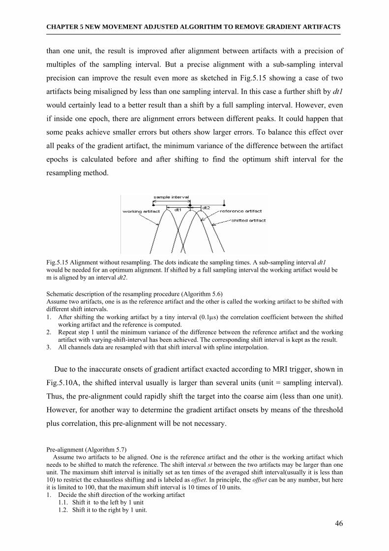
CHAPTER 5 NEW MOVEMENT ADJUSTED ALGORITHM TO REMOVE GRADIENT ARTIFACTS
46
than one unit, the result is improved after alignment between artifacts with a precision of
multiples of the sampling interval. But a precise alignment with a sub-sampling interval
precision can improve the result even more as sketched in Fig.5.15 showing a case of two
artifacts being misaligned by less than one sampling interval. In this case a further shift by dt1
would certainly lead to a better result than a shift by a full sampling interval. However, even
if inside one epoch, there are alignment errors between different peaks. It could happen that
some peaks achieve smaller errors but others show larger errors. To balance this effect over
all peaks of the gradient artifact, the minimum variance of the difference between the artifact
epochs is calculated before and after shifting to find the optimum shift interval for the
resampling method.
Fig.5.15 Alignment without resampling. The dots indicate the sampling times. A sub-sampling interval dt1 would be needed for an optimum alignment. If shifted by a full sampling interval the working artifact would be m is aligned by an interval dt2. Schematic description of the resampling procedure (Algorithm 5.6) Assume two artifacts, one is as the reference artifact and the other is called the working artifact to be shifted with different shift intervals. 1. After shifting the working artifact by a tiny interval (0.1μs) the correlation coefficient between the shifted
working artifact and the reference is computed. 2. Repeat step 1 until the minimum variance of the difference between the reference artifact and the working
artifact with varying-shift-interval has been achieved. The corresponding shift interval is kept as the result. 3. All channels data are resampled with that shift interval with spline interpolation.
Due to the inaccurate onsets of gradient artifact exacted according to MRI trigger, shown in
Fig.5.10A, the shifted interval usually is larger than several units (unit = sampling interval).
Thus, the pre-alignment could rapidly shift the target into the coarse aim (less than one unit).
However, for another way to determine the gradient artifact onsets by means of the threshold
plus correlation, this pre-alignment will be not necessary.
Pre-alignment (Algorithm 5.7) Assume two artifacts to be aligned. One is the reference artifact and the other is the working artifact which needs to be shifted to match the reference. The shift interval st between the two artifacts may be larger than one unit. The maximum shift interval is initially set as ten times of the averaged shift interval(usually it is less than 10) to restrict the exhaustless shifting and is labeled as offset. In principle, the offset can be any number, but here it is limited to 100, that the maximum shift interval is 10 times of 10 units. 1. Decide the shift direction of the working artifact
1.1. Shift it to the left by 1 unit 1.2. Shift it to the right by 1 unit.

CHAPTER 5 NEW MOVEMENT ADJUSTED ALGORITHM TO REMOVE GRADIENT ARTIFACTS
47
1.3. Calculate the variances of differences between the working artifact at the three positions (left, right, unchanged) and the reference.
1.4. If two variances of the three are the same the working artifact needs no shift. Return directly. If the left shifted variance is less than the unshifted variance, the shift direction is left. Otherwise right.
2. Estimate the step size. Step means the length of shifting per iteration counting by unit. In this phase, there are two defined steps, ten and one. For example, if the current step size is 10, the shift process will shift ten units per iteration.
3. Find the optimal shift interval (integer number of units) which deviates from the optimum no more than one unit. Do until all steps have been used. (if two steps, i = 1 to 2) 3.1. Shift the working artifact with step(i); 3.2 Find the optimal shift interval by calculating the minimum variance of difference between the reference
one and the shifted working one. 3.3 If found and the last step (inside step(2) repetition), break otherwise goto 3.1. End Do
4. Adjust the optimal shift interval by shifting it by ± 1 unit to test if the current position is the minimum variance position.
5. The working artifact is shifted by the determinate optimum shift interval.
Fast high precision alignment (Algorithm 5.8) The final step required after pre-alignment is the precise alignment in the sub-unit range (i.e. shifting it within one sampling interval). As before, there are the reference and the working artifact which need to be aligned. 1. Decide the shift direction.(right or left)
1.1. The working artifact is shifted to the left with 0.001. 1.2. The working artifact is shifted to the right with 0.001. 1.3. The variances are calculated for the difference between the working artifact at the three positions (left,
right, unchanged) and the reference. 1.4 If two variances of the three are the same the working artifact needs no shift. Return directly. If the left
shifted variance is less than the unshifted variance, the shift direction is left. Otherwise right. 2. Set three step values: 1/10, 1/100, and 1/1000 of the sampling interval (1 unit). step = [0.1 0.01 0.001] 3. Set up the initial shift interval (st = 0,i=1). 4. Do while st < 1
4.1. st = st + step(i) 4.2. The working artifact is shifted by st. 4.3. Compute the variance of the difference between the shifted working artifact and the reference artifact. 4.4. When the minimum variance is achieved and the actual step size is > 1/1000, the step size is replaced
with the smaller one in the step array and the optimization continues at 4.1. End do
5. Ensure that the optimized shift interval achieves the minimum variance of difference by backing one of the least step (0.001). Do until finding the minimum variance 5.1. st = st – 0.001; 5.2. The working artifact is shifted by st. 5.3. Compute the variance of the difference between the shifted working artifact and the reference artifact. 5.4. When the minimum of variance is achieved, exit.
End do
Comparing algorithm 5.6 to algorithm 5.8, the number of iterations for a single alignment is
clearly reduced from usually 1000 iteration (algorithm 5.6) to typically 30 (algorithm 5.8) for
the same resolution 0.0002 ms.
5.3.4.4 Subtraction
Finally, the averaged template is subtracted from the reference artifact to be removed. The
movement adapted averaging is individually conducted for each artifact to be removed.
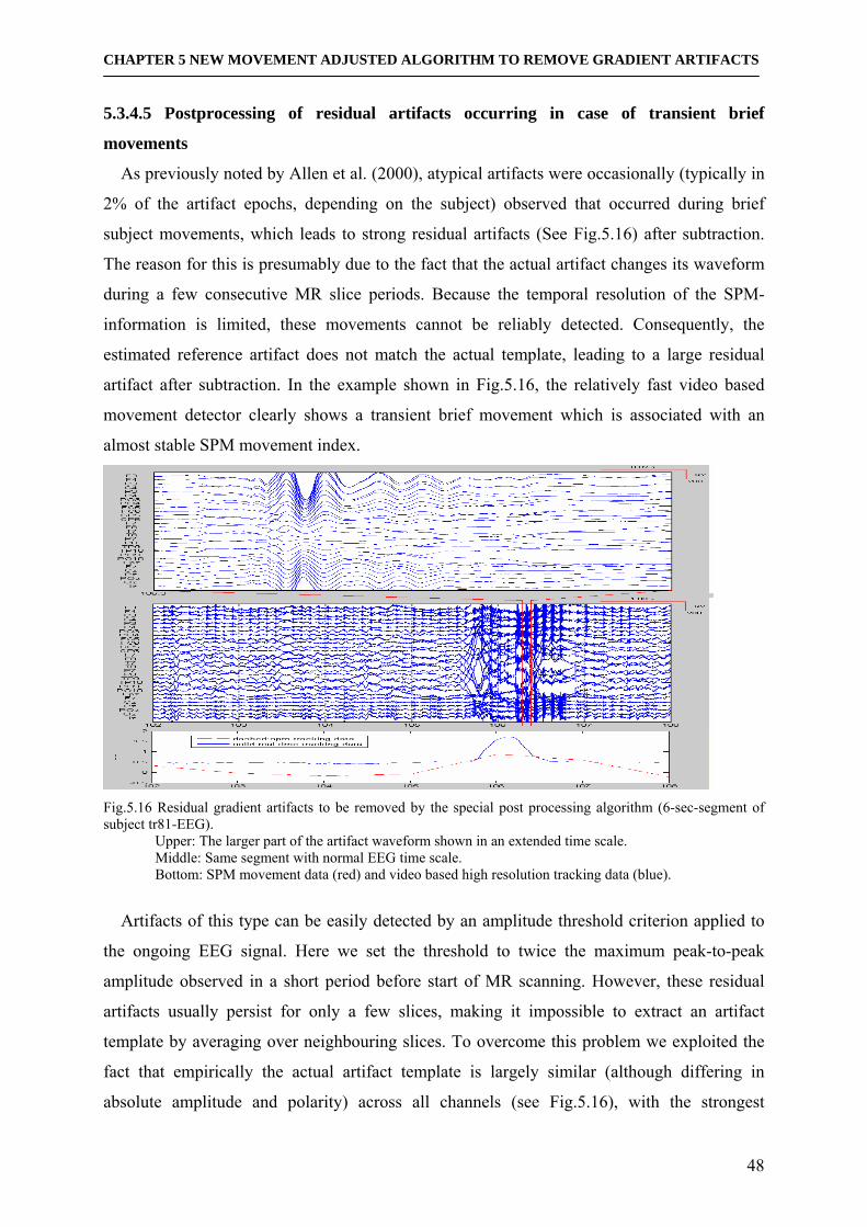
CHAPTER 5 NEW MOVEMENT ADJUSTED ALGORITHM TO REMOVE GRADIENT ARTIFACTS
48
5.3.4.5 Postprocessing of residual artifacts occurring in case of transient brief
movements
As previously noted by Allen et al. (2000), atypical artifacts were occasionally (typically in
2% of the artifact epochs, depending on the subject) observed that occurred during brief
subject movements, which leads to strong residual artifacts (See Fig.5.16) after subtraction.
The reason for this is presumably due to the fact that the actual artifact changes its waveform
during a few consecutive MR slice periods. Because the temporal resolution of the SPM-
information is limited, these movements cannot be reliably detected. Consequently, the
estimated reference artifact does not match the actual template, leading to a large residual
artifact after subtraction. In the example shown in Fig.5.16, the relatively fast video based
movement detector clearly shows a transient brief movement which is associated with an
almost stable SPM movement index.
Fig.5.16 Residual gradient artifacts to be removed by the special post processing algorithm (6-sec-segment of subject tr81-EEG).
Upper: The larger part of the artifact waveform shown in an extended time scale. Middle: Same segment with normal EEG time scale. Bottom: SPM movement data (red) and video based high resolution tracking data (blue).
Artifacts of this type can be easily detected by an amplitude threshold criterion applied to
the ongoing EEG signal. Here we set the threshold to twice the maximum peak-to-peak
amplitude observed in a short period before start of MR scanning. However, these residual
artifacts usually persist for only a few slices, making it impossible to extract an artifact
template by averaging over neighbouring slices. To overcome this problem we exploited the
fact that empirically the actual artifact template is largely similar (although differing in
absolute amplitude and polarity) across all channels (see Fig.5.16), with the strongest
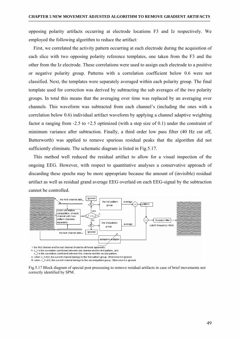
CHAPTER 5 NEW MOVEMENT ADJUSTED ALGORITHM TO REMOVE GRADIENT ARTIFACTS
49
opposing polarity artifacts occurring at electrode locations F3 and Iz respectively. We
employed the following algorithm to reduce the artifact:
First, we correlated the activity pattern occurring at each electrode during the acquisition of
each slice with two opposing polarity reference templates, one taken from the F3 and the
other from the Iz electrode. These correlations were used to assign each electrode to a positive
or negative polarity group. Patterns with a correlation coefficient below 0.6 were not
classified. Next, the templates were separately averaged within each polarity group. The final
template used for correction was derived by subtracting the sub averages of the two polarity
groups. In total this means that the averaging over time was replaced by an averaging over
channels. This waveform was subtracted from each channel’s (including the ones with a
correlation below 0.6) individual artifact waveform by applying a channel adaptive weighting
factor α ranging from -2.5 to +2.5 optimized (with a step size of 0.1) under the constraint of
minimum variance after subtraction. Finally, a third order low pass filter (40 Hz cut off,
Butterworth) was applied to remove spurious residual peaks that the algorithm did not
sufficiently eliminate. The schematic diagram is listed in Fig.5.17.
This method well reduced the residual artifact to allow for a visual inspection of the
ongoing EEG. However, with respect to quantitative analyses a conservative approach of
discarding these epochs may be more appropriate because the amount of (invisible) residual
artifact as well as residual grand average EEG overlaid on each EEG-signal by the subtraction
cannot be controlled.
Fig.5.17 Block diagram of special post processing to remove residual artifacts in case of brief movements not correctly identified by SPM.
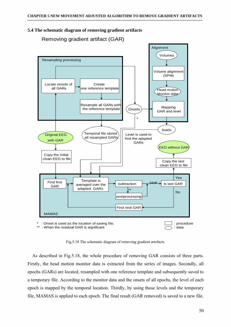
CHAPTER 5 NEW MOVEMENT ADJUSTED ALGORITHM TO REMOVE GRADIENT ARTIFACTS
50
5.4 The schematic diagram of removing gradient artifacts
Original EEGwith GAR
Createone reference template
Resample all GARs withthe reference template
Locate onsets ofall GARs
Temporal file storedall resampled GARs
Onsets
Volumes
Volume alignment(SPM)
Head motionMonitor data
MappingGAR and level
levels
Copy the initialclean EEG to file
Copy the last clean EEG to file
EEG without GAR
Find firstGAR
Template is averaged over the adapted GARs.
subtraction
Find next GAR
Removing gradient artifact (GAR)
Resampling processing
MAMAS
Alignment
Level is used to find the adapted
GARs
* : Onset is used as the location of saving file.** : When the residual GAR is significant.
: procedure: data
*
postprocessing
Is last GAR
No
Yes
**
save
Fig.5.18 The schematic diagram of removing gradient artefacts.
As described in Fig.5.18, the whole procedure of removing GAR consists of three parts.
Firstly, the head motion monitor data is extracted from the series of images. Secondly, all
epochs (GARs) are located, resampled with one reference template and subsequently saved to
a temporary file. According to the monitor data and the onsets of all epochs, the level of each
epoch is mapped by the temporal location. Thirdly, by using those levels and the temporary
file, MAMAS is applied to each epoch. The final result (GAR removed) is saved to a new file.
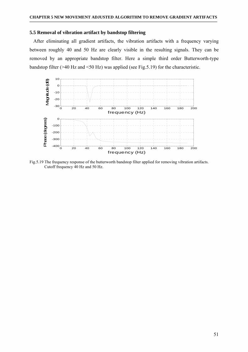
CHAPTER 5 NEW MOVEMENT ADJUSTED ALGORITHM TO REMOVE GRADIENT ARTIFACTS
51
5.5 Removal of vibration artifact by bandstop filtering
After eliminating all gradient artifacts, the vibration artifacts with a frequency varying
between roughly 40 and 50 Hz are clearly visible in the resulting signals. They can be
removed by an appropriate bandstop filter. Here a simple third order Butterworth-type
bandstop filter (>40 Hz and <50 Hz) was applied (see Fig.5.19) for the characteristic.
0 20 40 60 80 100 120 140 160 180 200-30
-20
-10
0
10
frequency (Hz)
Mag
nitu
de (d
B)
0 20 40 60 80 100 120 140 160 180 200-400
-300
-200
-100
0
frequency (Hz)
Pha
se (d
egre
es)
Fig.5.19 The frequency response of the butterworth bandstop filter applied for removing vibration artifacts.
Cutoff frequency 40 Hz and 50 Hz.
CHAPTER 6 NEW ALGORITHM TO REMOVE BCG ARTIFACTS
52
Chapter 6 New algorithm to remove BCG artifacts 6.1 New algorithm based on the Maximum Noise Fraction (MNF) method
6.1.1 Introduction of MNF
As described in detail in section 3.2, blind source separation (BSS) methods have been
applied by several groups for BCG removal (Briselli et al., 2006; Nakamura et al., 2006;
Mantini et al., 2007). The most popular BSS method in this field has been independent
component analysis (ICA).
The basic algorithm to apply this technique for the purpose of EEG-artifact removal is
described by the following generator model:
Assume an n-channel data matrix [ ]nxxxX ,...,, 21= to be a linear mixture of the source
matrix [ ]nsssS ,...,, 21= according to
SAX = (6.1)
with the n x n mixing matrix A defining the signal generation. Each component
kjxx ijTi ,...,1| == represents one real valued signal channel at k sampling times and
kjss ijTi ,...,1| == represents one real valued source component. To remove a certain artifact a
number of r components need to be identified that primarily represent artifact activity. These
components are then identified by a selection matrix T which is initialized as an n x n identity
matrix. For all indices i corresponding to an artifact component of S the element T(i,i) is set to
0, that represents the ith component is set to zero. Using this selection the artifact reduced
signal matrix X is reconstructed from the source matrix which is deduced as follows: 1−=⇔= XASSAX (6.2)
⎥⎥⎥⎥⎥⎥⎥⎥
⎦
⎤
⎢⎢⎢⎢⎢⎢⎢⎢
⎣
⎡
⋅==
0000
00000010
0001
ˆ
LL
MOMMLM
LL
LL
MLMMOM
LL
SSTS (6.3)
After setting zeros of several source components, the artifact reduced signal matrix X can be
estimated from the other source components.
ASX ˆˆ = (6.4)
According to eqs.6.2 and 6.3, the eq.6.4 can rewritten as
TAXASTAX 1ˆ −== (6.5)
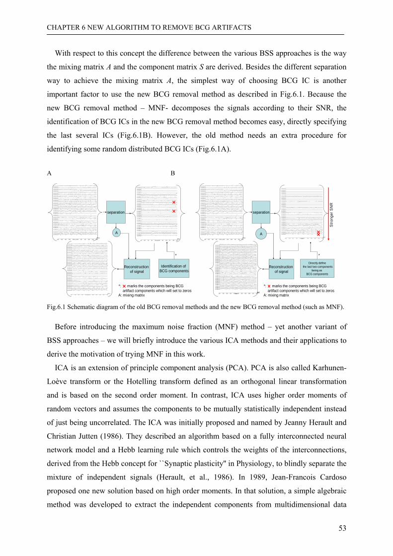
CHAPTER 6 NEW ALGORITHM TO REMOVE BCG ARTIFACTS
53
With respect to this concept the difference between the various BSS approaches is the way
the mixing matrix A and the component matrix S are derived. Besides the different separation
way to achieve the mixing matrix A, the simplest way of choosing BCG IC is another
important factor to use the new BCG removal method as described in Fig.6.1. Because the
new BCG removal method – MNF- decomposes the signals according to their SNR, the
identification of BCG ICs in the new BCG removal method becomes easy, directly specifying
the last several ICs (Fig.6.1B). However, the old method needs an extra procedure for
identifying some random distributed BCG ICs (Fig.6.1A).
A B
separation
A
Identification of BCG components
Reconstructionof signal
*
*: marks the components being BCG artifact components which will set to zeros
A: mixing matrix
separation
A
Directly definethe last two components
being as BCG components
Reconstructionof signal
*
*: marks the components being BCG artifact components which will set to zeros
A: mixing matrix
Stro
nger
SNR
Fig.6.1 Schematic diagram of the old BCG removal methods and the new BCG removal method (such as MNF).
Before introducing the maximum noise fraction (MNF) method – yet another variant of
BSS approaches – we will briefly introduce the various ICA methods and their applications to
derive the motivation of trying MNF in this work.
ICA is an extension of principle component analysis (PCA). PCA is also called Karhunen-
Loève transform or the Hotelling transform defined as an orthogonal linear transformation
and is based on the second order moment. In contrast, ICA uses higher order moments of
random vectors and assumes the components to be mutually statistically independent instead
of just being uncorrelated. The ICA was initially proposed and named by Jeanny Herault and
Christian Jutten (1986). They described an algorithm based on a fully interconnected neural
network model and a Hebb learning rule which controls the weights of the interconnections,
derived from the Hebb concept for ``Synaptic plasticity'' in Physiology, to blindly separate the
mixture of independent signals (Herault, et al., 1986). In 1989, Jean-Francois Cardoso
proposed one new solution based on high order moments. In that solution, a simple algebraic
method was developed to extract the independent components from multidimensional data
CHAPTER 6 NEW ALGORITHM TO REMOVE BCG ARTIFACTS
54
(Cardoso, 1989). Sources were identified by the estimation of the diagonalization
(orthonormality) of the weighted covariance of sensors. A variant of this method providing
more robust estimates was introduced by Souloumiac et al. (1991) and Souloumiac et al.
(1996). Comon (1994) developed an algorithm that minimizes the mutual information
between cumulants of components. A good introduction is presented by De Lathauwer et al.
(2000).
Up to now, based on different principles, several algorithms have been developed. The
most popular one is fastICA (Hyvaerinen, 1999) which is based on minimization or
maximization of an objective function, such as the likelihood, negentropy or mutual
information. When the function about mutual information is applied in fastICA, it is similar to
another often used algorithm - the infomax method (Bell et al., 1995; Lee et al., 1999) which
maximizes the mutual information. For the orthogonal tensor decomposition, the cumulant
based methods are developed by Comon(1994) and Cardoso(1999)with the different way to
find the mixing matrix, joint approximate diagonalization of eigenmatrices(JADE) (Cardoso)
and pairwise rotation (Comon). One version of this algorithm (proposed by Blaschke Tobias,
2004) performs a diagonalization of the cumulant tensors taking into account third- and
fourth-order cumulants simultaneously. The typical representative of this approach is JADE
(Cardoso, 1999) algorithm. Several ICA programs written in MATLAB can be downloaded
from internet2 directly.
Since some artifacts, such as eye movement and blink EEG artifacts (Joyce et al., 2004),
artifacts in magnetoencephalogram (MEG) (Barbati et al., 2004) and ocular artifacts in EEG
(Flexer et al., 2005), have been removed successfully with ICA, this type of BSS methods
became also the main tool of separation of BCG artifacts (Srivastava et al., 2005). FastICA
has been used in removing BCG artifacts in most cases. One idea (Briselli et al., 2006) , to
eliminate the influence of stochastic behavious (see above), was to carry out FastICA several
times with different initial conditions on the same EEG data. Then, using clustering
techniques EEG-components are achieved with a more statistical reliability. In another ICA
based approach (Nakamura et al., 2006) combined ICA with a subsequently applied high-pass
filter to solved the problem of residual BCG activity caused by non periodic BCG waveforms.
Recently ocular artifacts were removed together with BCG by ICA (Mantini et al., 2007).
2 Comon’s algorithm: http://www.i3s.unice.fr/~comon/codesICA.txt JADE: ftp://tsi.enst.fr/pub/jfc/Algo/Jade/jadeR.m FastICA: http://www.cis.hut.fi/projects/ica/fastica/loadcode.shtml
CHAPTER 6 NEW ALGORITHM TO REMOVE BCG ARTIFACTS
55
However, it is an inherent problem of all ICA (and also PCA) based approaches that the
more efficiently they remove the BCG the more some fraction of the underlying true EEG is
suppressed (Huiskamp et al., 2005) since the BCG and the EEG are not perfectly statistically
independent. Therefore, although ICA has been used widely in this field, in all realizations
some residual BCG artifacts still existed in the reconstructed data due to the uncompelete
orthogonal decomposition. As a second problem these applications are hardly suitable for an
automatic removal procedure because the independent components mainly carrying BCG
information need to be identified and marked interactively (Be´nar et al., 2003) or by a
correlation analysis including an additionally recorded electrocardiogram (ECG) (Srivastava
et al., 2005).
Therefore the goal and motivation of the work presented here was
(i) to develop a BSS method which better separates between the BCG and the EEG than
former ICA approaches (see above) and
(ii) to embed this procedure in a fully automatic removal concept.
As will be shown in the following, the maximum noise fraction (MNF) method, also named
maximum signal fraction (MSF) method (Hundley et al., 2001) largely meets this
requirements. Similar to PCA MNF is based on second order moment to separate signal,
however the two approaches are different in the way they create the mixing matrix out of
these moments. PCA derives the eigenvectors and eigenvalues of the covariance matrix of
observed signals, with each eigenvector (‘component’) corresponding to one eignevalue. In
contrast, MNF as a first step assumes the signal matrix X being an additive superposition of
some signal components (matrix P) to some noise components (matrix Q)
QPX +=
Assume orthogonality between P and Q. Each matrix is with n channel and m samples.
Given this model MNF creates the mixing matrix by searching the generalized eigenvectors
and eigenvalues of the covariance matrix of the signal parts and the covariance matrix of the
noise parts. This means, MNF explicitly addresses the problem of a signal contaminated by
noise. MNF was originally developed to denoise multispectral satellite images (Green et al.,
1988) and subsequently extended to the denoising of time-series (Anderle et al., 2001). MNF
finds a set of orthogonal basis vectors (later also labelled as ‘components’ or ‘ICs’) whose
directions represent the different generalized eigenvectors of the signal part and the noise. As
will be illustrated later, larger generalized eigenvalue means a stronger signal to noise ratio
CHAPTER 6 NEW ALGORITHM TO REMOVE BCG ARTIFACTS
56
(SNR). Usually, the noise is unknown and can only be approximated by the derivative of the
observed data. As will be shown in eqs.6.6 to 6.10 the mixing matrix can be determined by
the orthogonal eigenvectors of the signal’s derivative and the whitened signal derived from
the observed data.
In summary, MNF constructs a subspace of basis vectors maximizing the noise fraction of
separated components. As a side effect the basis vectors have a natural ordering according to
their noise fraction (= SNR). Having in mind the goal of introducing an automatic artifact
removal method this feature is in advantage of the randomly distributed ICs within the ICA
subspace, since the first or last few components (depending on the direction of ordering)
always carry the artifact information as long as the BCG artifact on average is the largest type
of artifact. In case of the – very rare – situation that if another artifact type is larger than the
BCG artifact, the EEG cannot be used anyhow due to its bad quality. Beyond this special
feature MNF is superior to the various popular ICA variants with regard to the segregation of
artifact activity from the EEG (see later in the results section).
The mathematical principle of MNF (Hundley et al., 2001) is deduced from the beginning
of the assumed EEG mixing model, the general production formulation. Another alternative
formulation, sum can replace the production (eq.6.1).
As introduced before (eqs.6.1 and 6.5) assume the two models to describe the generation of
the signal matrix X by mixing the components of the source matrix S according to SAX =
and alternatively to defining X as consisting of the true signal P plus additive orthogonal (not
necessarily white) noise Q as according to
QPX +=
Combining the two equations, P and Q may be written as
[ ]npppP ,,, 21 L= and ∑=
=m
iijij asp
1
, j=1,…,n
[ ]nqqqQ ,,, 21 L= and ∑+=
=n
miijij asq
1
, j=1,…n
with ija representing the elements of A in the ith row and the jth column and m is the
supposed number to construct P.
Here, 0=PQT and 0=QPT because of the assumption of orthogonality of P and Q.
So, QQPPQQQPPQPPQPQPXX TTTTTTTT +=+++=++= )()( (6.6)
We define the signal to noise ratio as
ψψψψ
ψψ
ψψ QQPP
QP
SNR TT
TT
00maxmax
≠≠==
(6.7)
CHAPTER 6 NEW ALGORITHM TO REMOVE BCG ARTIFACTS
57
With eq.6.6and eq.6.7, a new representation of SNR is derived.
ψψψψψψ
ψψψψ
ψψ QQQQXX
QQQQXXSNR TT
TTTT
TT
TTT −=
−=
≠≠ 00max)(max
)1(max0
−=⇒≠ ψψ
ψψψ QQ
XXSNR TT
TT
1max0
−=⇒≠ ψψ
ψψψ QQ
XXSNR TT
TT
(6.8)
Move 1 to the left of eq.6.8,
ψψψψ
ψ QQXXSNR TT
TT
0max1
≠=+
Defining SNR1 as SNR +1 leads to the following eq.6.9 which is the equivalent form of
eq.6.7.
ψψψψ
ψ QQXXSNR TT
TT
01 max≠
= (6.9)
The set of solutions to this problem are defined recursively by requiring all solution vectors to
be orthogonal in the sense that the inner product of the transformed data vectors by arbitrary
pairs of solution vectors is zero. i.e. 0=jT
i XX ψψ for all i≠j.
The solution to this problem leads to the generalized eigenvalue problem (see Kirby, 2001)
ψλψ QQXX TT = (6.10)
where ψ represents the eigenvector (or basis vector) and 1/λ is the noise fraction captured by
the basis vector. Hence, a set of orthogonal maximum noise fraction basis vectors possess a
natural ordering based on the noise fraction 1/λ.
Now, we need to estimate the covariance of Q, i.e. QQT from X.
Define sX as the set of observations X shifted forward by one time step. Then,
)()()()()()()()( sT
ssT
sssT
sssT
sT QQQQPPPPQPQPQPQPXXXXdXdX −−+−−≈−−+−−+=−−=
Assuming that the noise is temporally uncorrelated,, the following relations hold:
0== Ts
Ts QQQQ and
sTs
T QQQQ ≈ , )()(2 sT
sTT PPPPQQdXdX −−+≈
If the signal is smooth, then sPP− will be close to zero. The smoothness condition is well met
having in mind that the largest part of the BCG spectrum is mostly restricted to frequencies
below 20 Hz (see Fig.7.15) and thus clearly below the sampling frequency. Therefore, a good
estimation of QQT is dXdXT
21 .
Observed 1SNR and 2SNR , eq.6.11 has the same concept as eq.6.9.
CHAPTER 6 NEW ALGORITHM TO REMOVE BCG ARTIFACTS
58
ψψψψ
ψ dXdXXXSNRSNR TT
TT
012 max*2≠
==
(6.11)
Cichocki and Amari (2003) have shown that this eigen decomposition solves the mixing
problem given that the signal and the noise are orthogonal and that the one-lag
autocorrelations of the signal and the noise have different structures (that is, even in case of
non white noise).
Next, the mixing matrix A can be calculated as follows:
The singular value decomposition (SVD) of dX can be defined as TVUdX 111Σ= (6.12)
Where V1 and U1 are the unitary matrices.
Therefore IVVT
=11 and IUUT
=11 which will be used in eq.6.13.
For the whiten data has the same correlation property as the original data, by applying the
whitening transformation, 111−ΣV , to X and dX, the problem (eq.6.11) can be transformed into
ψψψψ
ψψψψ
ψψ T
TT
TTT
TTT XXdXVdXVXVXV ~~
maxmax01
1111
1
1111
11
0 ≠−−
−−
≠=
ΣΣΣΣ (6.13)
With
11
111
1111
111
11111
11
11111 UdXVUdXVVVUdXV IIVVT T
=Σ⎯⎯⎯ →⎯ΣΣ=Σ⎯⎯ →⎯ΣΣ=Σ −=ΣΣ−−=−− −
And
TTTITTT
TTTTIVVTTTTT
UdXVUdXV
UdXVUVVdXVT
T
111
1111
111
1
111
111
111111
111
1
11
111
11
=Σ⎯⎯⎯ →⎯ΣΣ=Σ⎯⎯ →⎯
ΣΣ=Σ⎯⎯ →⎯ΣΣ=Σ−=ΣΣ−−Σ=Σ
−−=−−
−
So,
IUUdXVdXV TTT ==ΣΣ −−11
1111
11 and 1
11~ −Σ= XVX
Thus, the generalized eigenvector problem transforms into the problem of SVD of X~ .
Back to eq.6.1, the mixing matrix A also can be represented by TAAA VUA Σ= .
Then
TAAA
TIUU
TAAA
TA
TAA
TTTT
VVdXdX
VUUVAAdSAdSAdXdXT
ATA 2, Σ=⎯⎯⎯⎯ →⎯
ΣΣ===Σ=Σ=
(6.14)
with the assumption of IdSdST = (Source components are the orthogonal components). AV
and AΣ can be computed by the eigenvector and eigenvalue decomposition of dXdX T .
Applying the whitening transformation, 1−Σ AAV to X yields
CHAPTER 6 NEW ALGORITHM TO REMOVE BCG ARTIFACTS
59
AAATAAAAAAA SUVVSUSAVXVX =ΣΣ=Σ=Σ= −−− 111ˆ . (6.15)
Using the assumption that Λ=SST (where Λ is the diagonal matrix carrying the squared
eigenvalues of S). AU is now found by
ATAA
TTA
T UUSUSUXX Λ==ˆˆ . (6.16)
AU is the eigenvector matrix of X .
According to eq.6.12 TTTTT VVVUUVdXdX 1
211111111 Σ=ΣΣ=
and eq.6.14 TAAA
T VVdXdX 2Σ=
Then TAAA
T VVVV 21
211 Σ=Σ (6.17)
Although eq.6.17 has a lot of solutions, we can give one solution of 1Σ=Σ A and 1VVA = .
Therefore, A is known ( 1VVA = and 1Σ=Σ A , and according to eq.6.16 AU is calculated).
With this approach, the independent components (S) have the nature character of SNR order,
that is the ranking of components according to their SNR. If BCG is the largest artifact, then it
will always be represented by the first or last (depending on the ordering direction)
component which is important for automatic removal. The detail algorithm of MNF is listed
in algorithm 6.1.
MNF approach (Algorithm 6.1) 1. Calculate the derivative dX of data X, i.e. the difference between the original data vector and the vector
resulting from the one-sample shift. 2. Compute the eigenvectors of the covariance of dX, leading to the matrices 1V (eigenvectors) and
1Σ (eigenvalues)
3. Create whitening matrix TV11
1−Σ .
4. Whiten data X according to XVX T1
11
~ −Σ= .
5. Compute the eigenvectors of the covariance of the whitened data X~ resulting in the matrices AU (the eigenvectors) and Λ (the eigenvalues)
6. Create the separation matrix as TTA VUA 1
11−Σ= .
7. Derive the source matrix as S=XA-1.
6.1.2 Application of MNF to BCG removal
Before removing BCG artifacts, gradient artifacts have to be removed by the MAMAS
method and vibration artifacts should also be suppressed as described before.
Once the source matrix has been derived (step 7 of algorithm 6.1), the last or first
(depending of the direction of ordering along the SNR) r components need to be suppressed
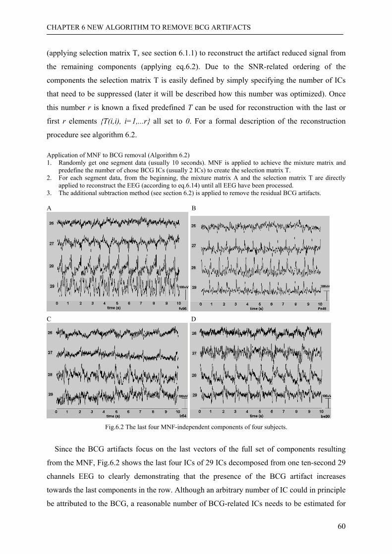
CHAPTER 6 NEW ALGORITHM TO REMOVE BCG ARTIFACTS
60
(applying selection matrix T, see section 6.1.1) to reconstruct the artifact reduced signal from
the remaining components (applying eq.6.2). Due to the SNR-related ordering of the
components the selection matrix T is easily defined by simply specifying the number of ICs
that need to be suppressed (later it will be described how this number was optimized). Once
this number r is known a fixed predefined T can be used for reconstruction with the last or
first r elements T(i,i), i=1,...r all set to 0. For a formal description of the reconstruction
procedure see algorithm 6.2. Application of MNF to BCG removal (Algorithm 6.2) 1. Randomly get one segment data (usually 10 seconds). MNF is applied to achieve the mixture matrix and
predefine the number of chose BCG ICs (usually 2 ICs) to create the selection matrix T. 2. For each segment data, from the beginning, the mixture matrix A and the selection matrix T are directly
applied to reconstruct the EEG (according to eq.6.14) until all EEG have been processed. 3. The additional subtraction method (see section 6.2) is applied to remove the residual BCG artifacts. A B
C D
Fig.6.2 The last four MNF-independent components of four subjects.
Since the BCG artifacts focus on the last vectors of the full set of components resulting
from the MNF, Fig.6.2 shows the last four ICs of 29 ICs decomposed from one ten-second 29
channels EEG to clearly demonstrating that the presence of the BCG artifact increases
towards the last components in the row. Although an arbitrary number of IC could in principle
be attributed to the BCG, a reasonable number of BCG-related ICs needs to be estimated for
CHAPTER 6 NEW ALGORITHM TO REMOVE BCG ARTIFACTS
61
instance by variance considerations (comparing the variance of the reconstructed EEG to the
variance of an EEG of the same subject but recorded outside the MR scanner) to balance the
losing of true EEG (if too many ICs are removed) with the amount of residual BCG artifacts
if not enough ICs have been removed. As will be shown later in the Results section, two or
three ICs achieve a sufficient BCG suppression. Minor residual BCG artifacts persisting after
that procedure can be further reduced by an additional subtraction method as described below.
6.1.3 Replacing the adaptive mixing matrix by a fixed matrix to reduce the computational load
Running the MNF analysis leads to a significant computational load which roughly
increases proportionally with the duration of the recorded EEG. Taking into account that in
typical MR-EEG recording sessions long periods of EEG (typically 30 min) need to be
processed, it is worth trying to reduce the numerical demands of MNF. Looking into the
details of the algorithm, the estimation of the mixing matrix A is the most complex part of it.
Therefore, the question arises, if it might be sufficient to take the mixing matrix A from the
first seconds of the recorded data and subsequently apply this (fixed) matrix to process the
full EEG period (as opposed to an adaptive concept which computes a new mixing matrix for
each of the sequence of short term epochs constituting the signal). In this case, the MNF
algorithm would be significantly speeded up.
To address this issue, a BCG identification signal (BIS) was derived from the EEG and
correlated with the components derived with the two alternative concepts (i.e. adaptive
mixing matrix vs. fixed mixing matrix). Components carrying BCG information (usually the
last or first few ICs, see before) will exhibit a large correlation with the BIS. If the
correlations of the BCG related ICs observed under the two compared regimes are similar,
then the algorithm using a fixed mixing matrix will achieve the same performance regarding
BCG removal as the adaptive version.
The BIS was derived as follows:
Empirically BCG artifacts are to some extent similar (although differing in amplitude and
polarity) across many channels. Therefore, we defined the first channel of 10-20-system
(which always showed a clear BCG artifact) as the initial BCG identification channel and
added or subtracted the other 28 channels according to the sign of their correlation with the
first channel. Finally, the resulting cumulated signal was normalized by the number of
channels. The schematic diagram of the generation of BIS is sketched in Fig.6.3 where the
modified channels are the original channels with their own signs (subtraction or addition).

CHAPTER 6 NEW ALGORITHM TO REMOVE BCG ARTIFACTS
62
CalculateCorrelationcoefficients
Channel 1
x
x
+1
-1
Averageall modified channelsBIS channel
>0
Yes
No
Channel 2
Channel N
...
Channel 1
ModifiedChannel 1
ModifiedChannel 2
ModifiedChannel N
...
: procedure: data
Fig.6.3 Schematic diagram of extracting the BCG identification signal (BIS).
To achieve acceptable results with a fixed rather than an adaptive mixing matrix A the last
(or first) components (which mainly represent BCG activity) as derived with the two
approaches should be equally correlated with the BIS to guarantee that the amount of BCG
that can be removed by dropping these components is comparable. Therefore we calculated
the correlation coefficients of each source component and the BIS of each subject’s EEG for
each of ten epochs of 10 sec duration. First, this was done using a fixed mixing matrix A for
all epochs of a subject with A being calculated from the first epoch for each sequence. Next,
we repeated the decomposition, however, this time applying the mixing matrix as derived
individually for each epoch.
The epoch-wise calculated mixing matrix can be replaced by the fixed matrix if the
distribution of the correlation coefficients over the source components is mainly identical in
the sense that (i) the last two components (later we show, that two components are sufficient
to remove the BCG) have the largest correlation of all and (ii) that the difference between
these correlations obtained for the two different approaches is smaller than the standard
deviation (over the subjects) of the adaptive variant. If these constraints are met the sources
later being dropped to remove the artifact will carry the same fraction of artifact activity.
6.1.4 Separating BCG and EEG: Comparison of MNF to ICA approaches
The correlations with the BIS signal were additionally used to compare MNF to two
popular ICA algorithms with respect to their capability to separate BCG from true EEG
CHAPTER 6 NEW ALGORITHM TO REMOVE BCG ARTIFACTS
63
activity. The stronger the correlations and the more the strongest correlations are focussed on
a few (last) source components the greater the power of the algorithm to extract specifically
BCG activity, i.e. to separate EEG and BCG.
The BIS was again derived from a 10 sec epoch selected randomly from the EEG recorded
in the scanner from each of the four subjects. Next, this epoch was decomposed by MNF, fast
ICA (Hyvaerinen, 1999) and JADE (Cardoso, 1998). Then, the resulting components were
ordered according to their correlation with the BIS in order to allow for a comparison between
the decomposition methods. These sets of correlation factors were statistically compared by
means of a two-sided t-test.
6.2 Additional Moving Average Subtraction algorithm to remove residual BCG activity
After using MNF, it is necessary to use subtraction to suppress the residual BCG artifacts.
The MNF technique can remove the BCG artifacts to a large degree but not completely.
Therefore, a template subtraction method (similar to the one used for gradient artifact
suppression) is applied to remove most of the residual BCG activity. Subtraction alone can
also not remove BCG artifacts completely (Negishi et al., 2004; Niazy et al., 2005).
Consequently – as will be demonstrated in the results chapter - the combination of the two
steps is needed to achieve a sufficient BCG artifact removal.
Similar to the gradient artifact algorithm, the subtraction algorithm averages over a limited
number of neighbouring BCG epochs and subtracts this average waveform from the actual
BCG epoch. In this context, the precise identification of the ECG (as the origin of the BCG
artifact) onset is critical for a correct alignment of the BCG epochs included in this procedure.
In principle the BIS could be used for this purpose as well but the ECG is better for the
following reasons: i) The peaks of the BIS are less strong. In some cases, they will be
misinterpreted due to the fact that two almost equally strong peaks occur in the BIS close to
each other (i.e. the one related to the R wave and a second related to the S wave of the ECG)
whereas the true ECG R wave is always much higher than S wave in the real ECG. Therefore,
the task of identifying the R-peak in the BIS is critical. ii) If head motions occur (especially
strong movements), the BCG onsets (by BIS) will be not detected because the waveforms are
corrupted by this motion. However, the ECG channels are not influenced by head motion (i.e.
the signal used to identify is perfect). iii) If there is an epileptic spike in the EEG, the BCG
onset may also not be detected because the spike often is the highest peak and the algorithm
just uses an amplitude threshold criterion.

CHAPTER 6 NEW ALGORITHM TO REMOVE BCG ARTIFACTS
64
Here, the two ECG channels (Ecg1 and Ecg2) are summed to serve as the reference channel
for this purpose. The BCG artifacts of the various EEG channels have different yet stable time
delays with respect to the ECG waveform. The ECG onset is defined as the time of the
maximum ECG peak which is usually the R wave of QRS complex. These ECG onsets are
then defined as the BCG onsets as well. With this procedure, the delays are constant part of
the channel dependent BCG waveform. Next, each individual BCG artifact’s template is
obtained by averaging over the BCG artifacts captured by a sliding window (rectangular
profile) whose width covers 50 ECG epochs. The current individual BCG artifact is
temporally located in the center of that sliding window. Finally, the average template is
subtracted from the individual BCG artifact. Further details of this procedure are described
below as algorithm 6.3 for ECG onset detection and as algorithm 6.5 for our subtraction.
Algorithm 6.4 describes the ECG onset detection and is used in the algorithm 6.3.
Detect sequence of ECG onsets (Algorithm 6.3) 1. Identify the first ECG onset and RR interval by Algorithm 6.4. A reference ECG model with RR length is
created from two ECG channels of EEG data at the first ECG onset by subtraction of the two ECG channels in order to enhance the characters of ECG (i.e. enlarge the waveforms of QRS).
2. Estimate the next onset. 2.1 Initially, the current onset is equal to the previous onset adding RR. 2.2 Create the current ECG model. 2.3 Compare the two ECG models’ peaks (QRS complex waves). If the distance between two peaks is not so
far (less than ¼ RR), goto 2.5. Otherwise, goto 2.4. 2.4 Relocate the current onset according to the peak position.
The new current onset = the current onset – (model peak position – reference model peak position). 2.5 Further adjust the current onset with correlation coefficient of the reference model and the current ECG
model with different shifted offset (usually range is 4RR± , increased step is one sample). The best
position is the maximum value of correlation coefficients. 3. Go to 2, until all ECG data have been processed. ECG start onset and RR estimator (Algorithm 6.4) 1. Extract the initial 3 second ECG data which are recorded at the two ECG channels (Ecg1 and Ecg2, See
section 4.3). 2. Find the ECG peaks. 2.1 Filter the ECG data with a highpass filter to remove the bias error. 2.2 Compute the threshold used to identify ECG peaks as 2/3 of averaged value of the local maximum
values of some epochs (½ second duration for each epoch). 2.3 Find the first onset which is larger than the threshold. For the next peak onset, the distance between this
position and the previous onset must larger than ½ second. 3. Compute the RR interval by averaging the difference values between the two onsets. Subtraction (Algorithm 6.5) 1. Detect ECG onsets with algorithm 6.3. 2. Adjust all BCG onsets: Each BCG onset is equal to the ECG onset subtracting ½ RR. Each BCG length is
equal to its onset adding RR. 3. Average the closer 50 BCG artifacts. The number of averaged artifacts can be reference to the other paper
about gradient artifacts removal. 4. Subtract this average from EEG. 5. Go to 3, until all BCG artifacts have been subtracted.
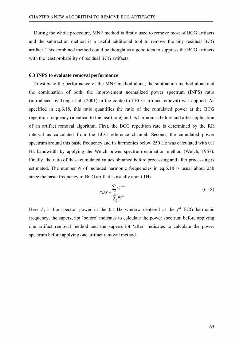
CHAPTER 6 NEW ALGORITHM TO REMOVE BCG ARTIFACTS
65
During the whole procedure, MNF method is firstly used to remove most of BCG artifacts
and the subtraction method is a useful additional tool to remove the tiny residual BCG
artifact. This combined method could be thought as a good idea to suppress the BCG artifacts
with the least probability of residual BCG artifacts.
6.3 INPS to evaluate removal performance
To estimate the performance of the MNF method alone, the subtraction method alone and
the combination of both, the improvement normalized power spectrum (INPS) ratio
(introduced by Tong et al. (2001) in the context of ECG artifact removal) was applied. As
specified in eq.6.18, this ratio quantifies the ratio of the cumulated power at the BCG
repetition frequency (identical to the heart rate) and its harmonics before and after application
of an artifact removal algorithm. First, the BCG repetition rate is determined by the RR
interval as calculated from the ECG reference channel. Second, the cumulated power
spectrum around this basic frequency and its harmonics below 250 Hz was calculated with 0.1
Hz bandwidth by applying the Welch power spectrum estimation method (Welch, 1967).
Finally, the ratio of these cumulated values obtained before processing and after processing is
estimated. The number N of included harmonic frequencies in eq.6.18 is usual about 250
since the basic frequency of BCG artifact is usually about 1Hz.
∑
∑
=
== N
j
afterj
N
j
beforej
P
PINPS
0
0 (6.18)
Here Pj is the spectral power in the 0.1-Hz window centered at the jth ECG harmonic
frequency, the superscript ‘before’ indicates to calculate the power spectrum before applying
one artifact removal method and the superscript ‘after’ indicates to calculate the power
spectrum before applying one artifact removal method.
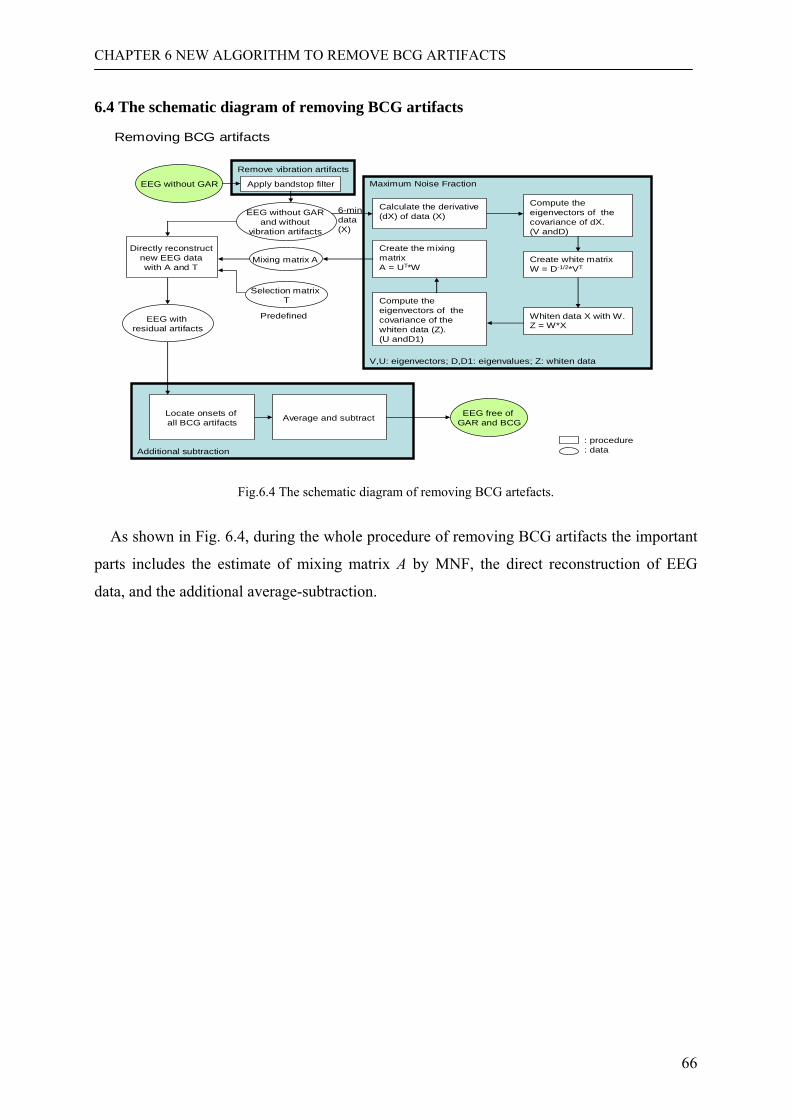
CHAPTER 6 NEW ALGORITHM TO REMOVE BCG ARTIFACTS
66
6.4 The schematic diagram of removing BCG artifacts
EEG without GAR Apply bandstop filter
EEG without GAR and without
vibration artifacts
Mixing matrix A Directly reconstruct
new EEG datawith A and T
Average and subtract EEG free of GAR and BCG
EEG withresidual artifacts
Locate onsets of all BCG artifacts
6-min data(X)
Selection matrixT
Predefined
Additional subtraction
Removing BCG artifacts
: procedure: data
Maximum Noise Fraction
Calculate the derivative (dX) of data (X)
Compute the eigenvectors of the covariance of dX.(V andD)
Create white matrix W = D-1/2*VT
Whiten data X with W.Z = W*X
Compute the eigenvectors of the covariance of the whiten data (Z).(U andD1)
Create the mixingmatrix A = UT*W
V,U: eigenvectors; D,D1: eigenvalues; Z: whiten data
Remove vibration artifacts
Fig.6.4 The schematic diagram of removing BCG artefacts.
As shown in Fig. 6.4, during the whole procedure of removing BCG artifacts the important
parts includes the estimate of mixing matrix A by MNF, the direct reconstruction of EEG
data, and the additional average-subtraction.
CHAPTER 7 RESULTS
67
Chapter 7 Results 7.1 Gradient artifacts, MAMAS-algorithm: Evaluation and Comparison with the MAS
algorithm
7.1.1 Gradient artifact resampling
Fig.7.1A shows the average standard deviation of the differences (subsequently called
‘resampling error’) between the simulated reference artifact and the 30 resampled jittered
templates observed at the different relative temporal resolution values δt (δt=1 representing
the original sampling interval). It meets the EEG amplifier noise level of about a uV at a
relative temporal resolution of approximately δt = .005 (i.e. an absolute resolution of .001
ms). Bearing in mind that even stronger artifacts cannot be ruled out around the artifact peaks,
we set δtopt to .001 (corresponding to an absolute resolution of .0002 msec) for the removal
algorithm. The optimized resampling algorithm needs a maximum of 30 iterations to find the
optimal shift interval at this resolution. In principle this procedure is comparable to an
upsampling of the gradient artifact to 5 MHz and aligning it to the reference artifact, however
avoiding the boost in data volume and computational load.
Fig.7.1B shows an extreme example to illustrate in the time domain how much reduction in
residual artifact activity can be achieved by replacing the upsampling by the resampling
algorithm. Visually the improvement is most prominent for high frequency components
exceeding 100 Hz, but the signal’s power spectrum is an average over 10 6-sec-epochs
recorded at electrode position Fp1 of one subject. Fig.7.1C demonstrates an artifact reduction
that extends over all harmonics of the gradient repetition frequency (10 Hz in this case).
Besides an improved artifact removal we observed a reduction of computing time by a factor
of 4 and at the same time a reduction of memory usage by a factor of 10 with resampling
compared to upsampling to 50 KHZ. In both cases interpolation was done by means of a
cubic spline function. Since the EEG- and the fMRI-clocks were not synchronized, the
amount of shifting needed leading to an optimal sampling timing (in case of re-sampling) was
randomly distributed over the original sampling interval or 0.2 ms; the average number of
steps to find this optimum was 15.
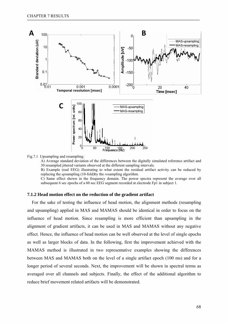
CHAPTER 7 RESULTS
68
Fig.7.1 Upsampling and resampling:
A) Average standard deviation of the differences between the digitally simulated reference artifact and 30 resampled jittered variants observed at the different sampling intervals. B) Example (real EEG) illustrating to what extent the residual artifact activity can be reduced by replacing the upsampling (10-fold)by the resampling algorithm. C) Same effect shown in the frequency domain. The power spectra represent the average over all subsequent 6 sec epochs of a 60 sec EEG segment recorded at electrode Fp1 in subject 1.
7.1.2 Head motion effect on the reduction of the gradient artifact
For the sake of testing the influence of head motion, the alignment methods (resampling
and upsampling) applied in MAS and MAMAS should be identical in order to focus on the
influence of head motion. Since resampling is more efficient than upsampling in the
alignment of gradient artifacts, it can be used in MAS and MAMAS without any negative
effect. Hence, the influence of head motion can be well observed at the level of single epochs
as well as larger blocks of data. In the following, first the improvement achieved with the
MAMAS method is illustrated in two representative examples showing the differences
between MAS and MAMAS both on the level of a single artifact epoch (100 ms) and for a
longer period of several seconds. Next, the improvement will be shown in spectral terms as
averaged over all channels and subjects. Finally, the effect of the additional algorithm to
reduce brief movement related artifacts will be demonstrated.
A
C
B
Temporal resolution [msec]
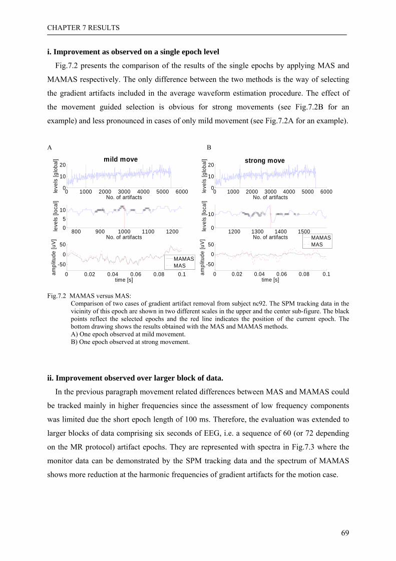
CHAPTER 7 RESULTS
69
i. Improvement as observed on a single epoch level
Fig.7.2 presents the comparison of the results of the single epochs by applying MAS and
MAMAS respectively. The only difference between the two methods is the way of selecting
the gradient artifacts included in the average waveform estimation procedure. The effect of
the movement guided selection is obvious for strong movements (see Fig.7.2B for an
example) and less pronounced in cases of only mild movement (see Fig.7.2A for an example).
A B
0 1000 2000 3000 4000 5000 60000
10
20
leve
ls [g
loba
l]
No. of artifacts
800 900 1000 1100 120005
10
leve
ls [l
ocal
]
No. of artifacts
0 0.02 0.04 0.06 0.08 0.1
-50
0
50
ampl
itude
[uV]
time [s]
MAMASMAS
mild move
0 1000 2000 3000 4000 5000 60000
10
20
leve
ls [g
loba
l]No. of artifacts
1200 1300 1400 15000
10
leve
ls [l
ocal
]
No. of artifacts
0 0.02 0.04 0.06 0.08 0.1
-50
0
50
ampl
itude
[uV]
time [s]
MAMASMAS
strong move
Fig.7.2 MAMAS versus MAS:
Comparison of two cases of gradient artifact removal from subject nc92. The SPM tracking data in the vicinity of this epoch are shown in two different scales in the upper and the center sub-figure. The black points reflect the selected epochs and the red line indicates the position of the current epoch. The bottom drawing shows the results obtained with the MAS and MAMAS methods. A) One epoch observed at mild movement. B) One epoch observed at strong movement.
ii. Improvement observed over larger block of data.
In the previous paragraph movement related differences between MAS and MAMAS could
be tracked mainly in higher frequencies since the assessment of low frequency components
was limited due the short epoch length of 100 ms. Therefore, the evaluation was extended to
larger blocks of data comprising six seconds of EEG, i.e. a sequence of 60 (or 72 depending
on the MR protocol) artifact epochs. They are represented with spectra in Fig.7.3 where the
monitor data can be demonstrated by the SPM tracking data and the spectrum of MAMAS
shows more reduction at the harmonic frequencies of gradient artifacts for the motion case.
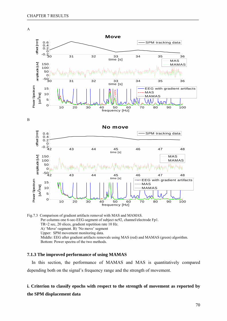
CHAPTER 7 RESULTS
70
A
30 31 32 33 34 35 36-0.2
00.20.40.6
offs
et [m
m]
time [s]
SPM tracking data
30 31 32 33 34 35 36-50
050
100150
ampl
itude
[uV]
time [s]
MASMAMAS
10 20 30 40 50 60 70 80 90 1000
5
10
15
frequency [Hz]
Power
Spe
ctru
m
[uV2 /
Hz]
EEG with gradient artifactsMASMAMAS
Move
B
42 43 44 45 46 47 48-0.2
00.20.40.6
offs
et [m
m]
time [s]
SPM tracking data
42 43 44 45 46 47 48-50
050
100150
ampl
itude
[uV]
time [s]
MASMAMAS
10 20 30 40 50 60 70 80 90 1000
5
10
15
frequency [Hz]
Pow
er S
pect
rum
[uV2 /H
z]
EEG with gradient artifactsMASMAMAS
No move
Fig.7.3 Comparison of gradient artifacts removal with MAS and MAMAS.
Per columns one 6-sec-EEG-segment of subject nc92, channel/electrode Fp1. TR=2 sec, 20 slices, gradient repetition rate 10 Hz. A) ‘Move’-segment. B) ‘No move’ segment Upper: SPM movement monitoring data. Middle: EEG after gradient artifacts removals using MAS (red) and MAMAS (green) algorithm. Bottom: Power spectra of the two methods.
7.1.3 The improved performance of using MAMAS
In this section, the performance of MAMAS and MAS is quantitatively compared
depending both on the signal’s frequency range and the strength of movement.
i. Criterion to classify epochs with respect to the strength of movement as reported by
the SPM displacement data
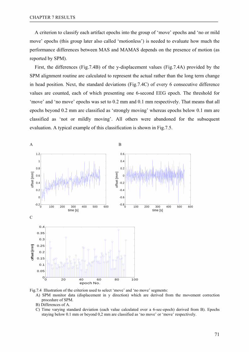
CHAPTER 7 RESULTS
71
A criterion to classify each artifact epochs into the group of ‘move’ epochs and ‘no or mild
move’ epochs (this group later also called ‘motionless’) is needed to evaluate how much the
performance differences between MAS and MAMAS depends on the presence of motion (as
reported by SPM).
First, the differences (Fig.7.4B) of the y-displacement values (Fig.7.4A) provided by the
SPM alignment routine are calculated to represent the actual rather than the long term change
in head position. Next, the standard deviations (Fig.7.4C) of every 6 consecutive difference
values are counted, each of which presenting one 6-second EEG epoch. The threshold for
‘move’ and ‘no move’ epochs was set to 0.2 mm and 0.1 mm respectively. That means that all
epochs beyond 0.2 mm are classified as ‘strongly moving’ whereas epochs below 0.1 mm are
classified as ‘not or mildly moving’. All others were abandoned for the subsequent
evaluation. A typical example of this classification is shown in Fig.7.5.
A B
0 100 200 300 400 500 600-0.2
0
0.2
0.4
0.6
0.8
1
1.2
time [s]
offs
et [m
m]
0 100 200 300 400 500 600-0.8
-0.6
-0.4
-0.2
0
0.2
0.4
0.6
time [s]
offs
et [m
m]
C
0 20 40 60 80 1000
0.05
0.1
0.15
0.2
0.25
0.3
0.35
0.4
epoch No.
offs
et [m
m]
Fig.7.4 Illustration of the criterion used to select ‘move’ and ‘no move’ segments:
A) SPM monitor data (displacement in y direction) which are derived from the movement correction procedure of SPM.
B) Differences of A. C) Time varying standard deviation (each value calculated over a 6-sec-epoch) derived from B). Epochs
staying below 0.1 mm or beyond 0,2 mm are classified as ‘no move’ or ‘move’ respectively.
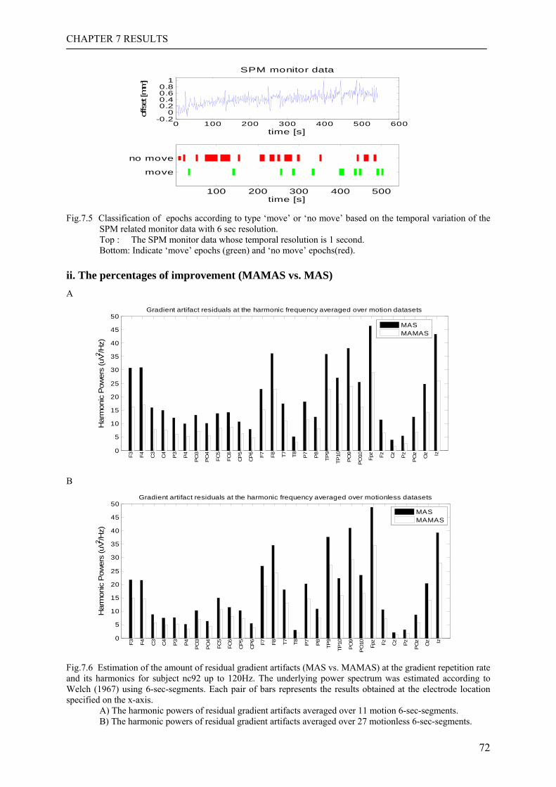
CHAPTER 7 RESULTS
72
0 100 200 300 400 500 600-0.2
00.20.40.60.8
1
offset [m
m]
time [s]
SPM monitor data
100 200 300 400 500
move
no move
time [s] Fig.7.5 Classification of epochs according to type ‘move’ or ‘no move’ based on the temporal variation of the
SPM related monitor data with 6 sec resolution. Top : The SPM monitor data whose temporal resolution is 1 second. Bottom: Indicate ‘move’ epochs (green) and ‘no move’ epochs(red).
ii. The percentages of improvement (MAMAS vs. MAS) A
0
5
10
15
20
25
30
35
40
45
50Gradient artifact residuals at the harmonic frequency averaged over motion datasets
Har
mon
ic P
ower
s (u
V2 /Hz)
F3 F4 C3
C4
P3
P4
PO
3
PO
4
FC5
FC6
CP
5
CP
6 F7 F8 T7 T8 P7
P8
TP9
TP10
PO
9
PO
10 Fpz Fz Cz
Pz
PO
z
Oz Iz
MASMAMAS
B
0
5
10
15
20
25
30
35
40
45
50Gradient artifact residuals at the harmonic frequency averaged over motionless datasets
Har
mon
ic P
ower
s (u
V2 /Hz)
F3 F4 C3
C4
P3
P4
PO
3
PO
4
FC5
FC6
CP
5
CP
6 F7 F8 T7 T8 P7
P8
TP9
TP10
PO
9
PO
10 Fpz Fz Cz
Pz
PO
z
Oz Iz
MASMAMAS
Fig.7.6 Estimation of the amount of residual gradient artifacts (MAS vs. MAMAS) at the gradient repetition rate and its harmonics for subject nc92 up to 120Hz. The underlying power spectrum was estimated according to Welch (1967) using 6-sec-segments. Each pair of bars represents the results obtained at the electrode location specified on the x-axis.
A) The harmonic powers of residual gradient artifacts averaged over 11 motion 6-sec-segments. B) The harmonic powers of residual gradient artifacts averaged over 27 motionless 6-sec-segments.
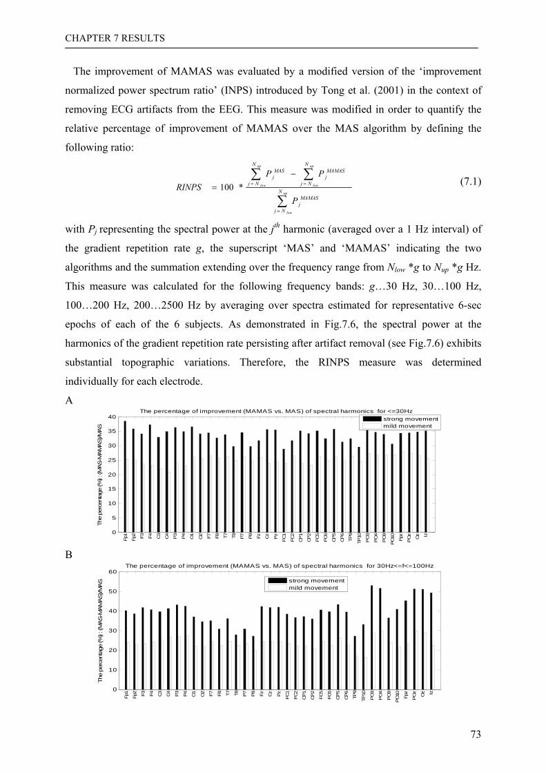
CHAPTER 7 RESULTS
73
The improvement of MAMAS was evaluated by a modified version of the ‘improvement
normalized power spectrum ratio’ (INPS) introduced by Tong et al. (2001) in the context of
removing ECG artifacts from the EEG. This measure was modified in order to quantify the
relative percentage of improvement of MAMAS over the MAS algorithm by defining the
following ratio:
∑
∑∑
=
==
−=
up
low
up
low
up
low
N
Nj
MAMASj
N
Nj
MAMASj
N
Nj
MASj
P
PPRINPS *100 (7.1)
with Pj representing the spectral power at the jth harmonic (averaged over a 1 Hz interval) of
the gradient repetition rate g, the superscript ‘MAS’ and ‘MAMAS’ indicating the two
algorithms and the summation extending over the frequency range from Nlow *g to Nup *g Hz.
This measure was calculated for the following frequency bands: g…30 Hz, 30…100 Hz,
100…200 Hz, 200…2500 Hz by averaging over spectra estimated for representative 6-sec
epochs of each of the 6 subjects. As demonstrated in Fig.7.6, the spectral power at the
harmonics of the gradient repetition rate persisting after artifact removal (see Fig.7.6) exhibits
substantial topographic variations. Therefore, the RINPS measure was determined
individually for each electrode.
A
0
5
10
15
20
25
30
35
40The percentage of improvement (MAMAS vs. MAS) of spectral harmonics for <=30Hz
The
perc
enta
ge (%
) : (M
AS-M
AM
AS)/M
AS
Fp1
Fp2 F3 F4 C3
C4
P3
P4
O1
O2 F7 F8 T7 T8 P7
P8 Fz Cz
Pz
FC1
FC2
CP1
CP2
FC5
FC6
CP5
CP6
TP9
TP10
PO
3
PO
4
PO
9
PO
10 Fpz
PO
z
Oz Iz
strong movementmild movement
B
0
10
20
30
40
50
60The percentage of improvement (MAMAS vs. MAS) of spectral harmonics for 30Hz<=f<=100Hz
The
perc
enta
ge (%
) : (M
AS-M
AM
AS)/M
AS
Fp1
Fp2 F3 F4 C3
C4
P3
P4
O1
O2 F7 F8 T7 T8 P7
P8 Fz Cz
Pz
FC1
FC2
CP1
CP2
FC5
FC6
CP5
CP6
TP9
TP10
PO
3
PO
4
PO
9
PO
10 Fpz
PO
z
Oz Iz
strong movementmild movement
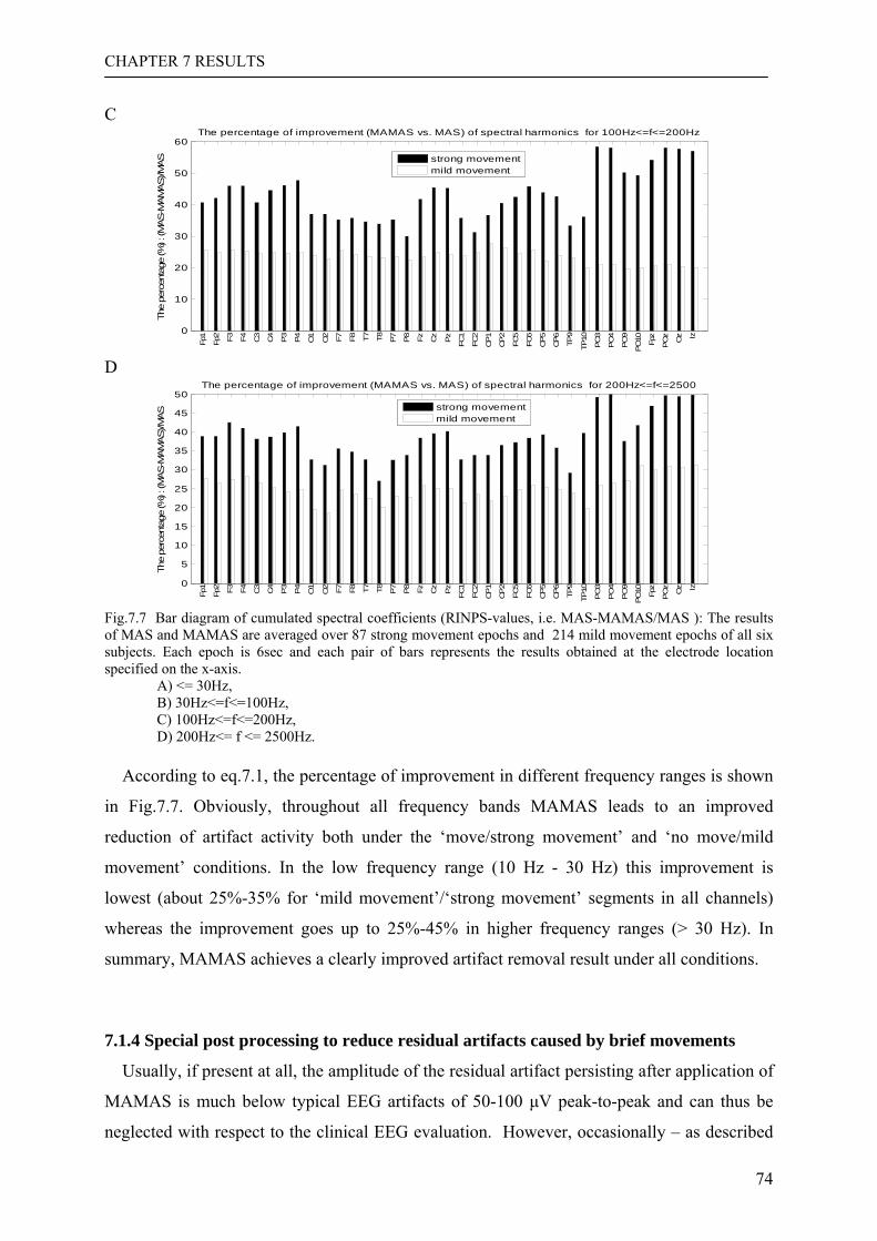
CHAPTER 7 RESULTS
74
C
0
10
20
30
40
50
60The percentage of improvement (MAMAS vs. MAS) of spectral harmonics for 100Hz<=f<=200Hz
The
perc
enta
ge (%
) : (M
AS-M
AM
AS)/M
AS
Fp1
Fp2 F3 F4 C3
C4
P3
P4
O1
O2 F7 F8 T7 T8 P7
P8 Fz Cz
Pz
FC1
FC2
CP1
CP2
FC5
FC6
CP5
CP6
TP9
TP10
PO
3
PO
4
PO
9
PO
10 Fpz
PO
z
Oz Iz
strong movementmild movement
D
0
5
10
15
20
25
30
35
40
45
50The percentage of improvement (MAMAS vs. MAS) of spectral harmonics for 200Hz<=f<=2500
The
perc
enta
ge (%
) : (M
AS-M
AM
AS)/M
AS
Fp1
Fp2 F3 F4 C3
C4
P3
P4
O1
O2 F7 F8 T7 T8 P7
P8 Fz Cz
Pz
FC1
FC2
CP1
CP2
FC5
FC6
CP5
CP6
TP9
TP10
PO
3
PO
4
PO
9
PO
10 Fpz
PO
z
Oz Iz
strong movementmild movement
Fig.7.7 Bar diagram of cumulated spectral coefficients (RINPS-values, i.e. MAS-MAMAS/MAS ): The results of MAS and MAMAS are averaged over 87 strong movement epochs and 214 mild movement epochs of all six subjects. Each epoch is 6sec and each pair of bars represents the results obtained at the electrode location specified on the x-axis.
A) <= 30Hz, B) 30Hz<=f<=100Hz, C) 100Hz<=f<=200Hz, D) 200Hz<= f <= 2500Hz.
According to eq.7.1, the percentage of improvement in different frequency ranges is shown
in Fig.7.7. Obviously, throughout all frequency bands MAMAS leads to an improved
reduction of artifact activity both under the ‘move/strong movement’ and ‘no move/mild
movement’ conditions. In the low frequency range (10 Hz - 30 Hz) this improvement is
lowest (about 25%-35% for ‘mild movement’/‘strong movement’ segments in all channels)
whereas the improvement goes up to 25%-45% in higher frequency ranges (> 30 Hz). In
summary, MAMAS achieves a clearly improved artifact removal result under all conditions.
7.1.4 Special post processing to reduce residual artifacts caused by brief movements
Usually, if present at all, the amplitude of the residual artifact persisting after application of
MAMAS is much below typical EEG artifacts of 50-100 μV peak-to-peak and can thus be
neglected with respect to the clinical EEG evaluation. However, occasionally – as described
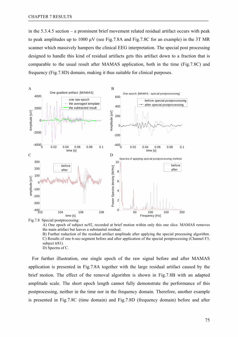
CHAPTER 7 RESULTS
75
in the 5.3.4.5 section – a prominent brief movement related residual artifact occurs with peak
to peak amplitudes up to 1000 μV (see Fig.7.8A and Fig.7.8C for an example) in the 3T MR
scanner which massively hampers the clinical EEG interpretation. The special post processing
designed to handle this kind of residual artifacts gets this artifact down to a fraction that is
comparable to the usual result after MAMAS application, both in the time (Fig.7.8C) and
frequency (Fig.7.8D) domain, making it thus suitable for clinical purposes.
A B
0 0.02 0.04 0.06 0.08 0.1-4000
-2000
0
2000
4000
time [s]
Am
plitu
de [u
V]
One gradient artifact: [MAMAS]
one raw epochthe averaged templatethe subtracted result
0 0.02 0.04 0.06 0.08 0.1-400
-200
0
200
400
600
time [s]
Am
plitu
de [u
V]
One epoch: [MAMAS - special postprocessing]
before special postprocessingafter special postprocessing
C D
102 104 106 108-400
-300
-200
-100
0
100
200
300
time [s]
ampl
itude
[uV
]
beforeafter
50 100 150 2000
2
4
6
8
10
Frequency [Hz]
Pow
er S
pect
ra d
ensi
ty [W
/Hz]
Spectra of applying special postprocessing method
beforeafter
Fig.7.8 Special postprocessing:
A) One epoch of subject nc92, recorded at brief motion within only this one slice. MAMAS removes the main artifact but leaves a substantial residual. B) Further reduction of the residual artifact amplitude after applying the special processing algorithm. C) Results of one 6-sec-segment before and after application of the special postprocessing (Channel F3, subject tr81). D) Spectra of C.
For further illustration, one single epoch of the raw signal before and after MAMAS
application is presented in Fig.7.8A together with the large residual artifact caused by the
brief motion. The effect of the removal algorithm is shown in Fig.7.8B with an adapted
amplitude scale. The short epoch length cannot fully demonstrate the performance of this
postprocessing, neither in the time nor in the frequency domain. Therefore, another example
is presented in Fig.7.8C (time domain) and Fig.7.8D (frequency domain) before and after
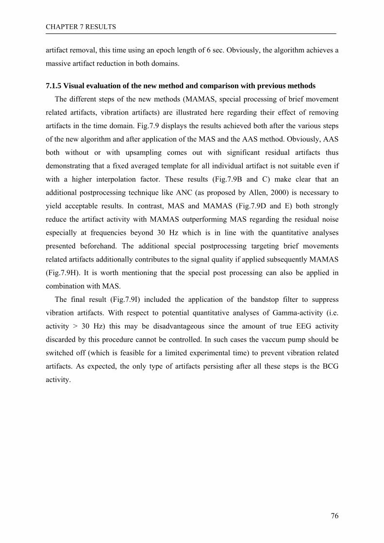
CHAPTER 7 RESULTS
76
artifact removal, this time using an epoch length of 6 sec. Obviously, the algorithm achieves a
massive artifact reduction in both domains.
7.1.5 Visual evaluation of the new method and comparison with previous methods
The different steps of the new methods (MAMAS, special processing of brief movement
related artifacts, vibration artifacts) are illustrated here regarding their effect of removing
artifacts in the time domain. Fig.7.9 displays the results achieved both after the various steps
of the new algorithm and after application of the MAS and the AAS method. Obviously, AAS
both without or with upsampling comes out with significant residual artifacts thus
demonstrating that a fixed averaged template for all individual artifact is not suitable even if
with a higher interpolation factor. These results (Fig.7.9B and C) make clear that an
additional postprocessing technique like ANC (as proposed by Allen, 2000) is necessary to
yield acceptable results. In contrast, MAS and MAMAS (Fig.7.9D and E) both strongly
reduce the artifact activity with MAMAS outperforming MAS regarding the residual noise
especially at frequencies beyond 30 Hz which is in line with the quantitative analyses
presented beforehand. The additional special postprocessing targeting brief movements
related artifacts additionally contributes to the signal quality if applied subsequently MAMAS
(Fig.7.9H). It is worth mentioning that the special post processing can also be applied in
combination with MAS.
The final result (Fig.7.9I) included the application of the bandstop filter to suppress
vibration artifacts. With respect to potential quantitative analyses of Gamma-activity (i.e.
activity > 30 Hz) this may be disadvantageous since the amount of true EEG activity
discarded by this procedure cannot be controlled. In such cases the vaccum pump should be
switched off (which is feasible for a limited experimental time) to prevent vibration related
artifacts. As expected, the only type of artifacts persisting after all these steps is the BCG
activity.
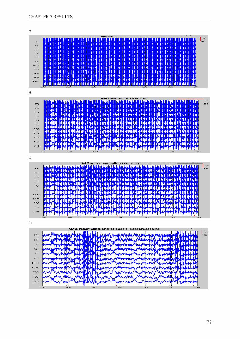
CHAPTER 7 RESULTS
77
A
B
C
D
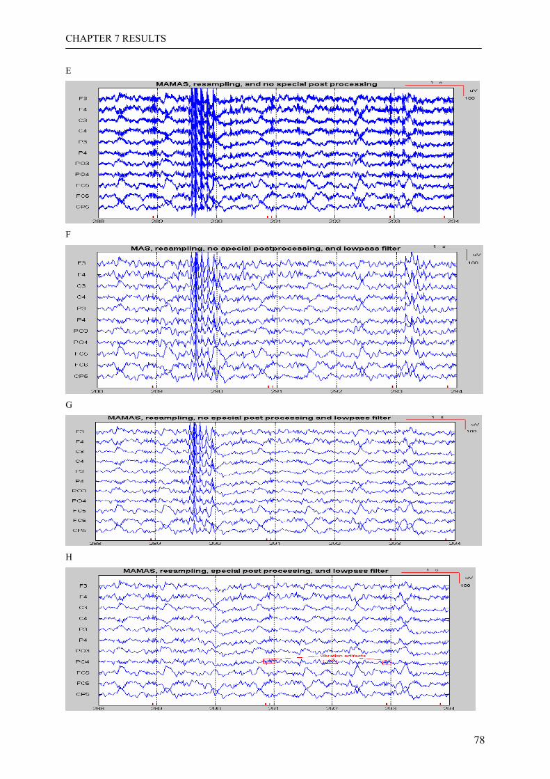
CHAPTER 7 RESULTS
78
E
F
G
H
CHAPTER 7 RESULTS
79
I
Fig.7.9 Comparison of different processing steps (as indicated) as applied to one 6-sec-EEG-segment of subject nc92.
A) Raw EEG channels (F3, F4, C3, C4, P3, P4, PO3, PO4, FC5, FC6, CP5) recorded during MR scanning.
B) AAS (Allen et. al., 2000) without upsampling. C) AAS with upsampling (factor 4). D) MAS with resampling, without special post processing. E) MAMAS with resampling, without special post processing. F) MAS with resampling, without special post processing, low pass filtering with 120 Hz cutoff
frequency. G) MAMAS with resampling, without special post processing, low pass filtering with 120 Hz cutoff
frequency. H) MAMAS with resampling, special post processing, low pass filtering with 120 Hz cutoff frequency. I) MAMAS with resampling, special post processing, low pass filtering with 120 Hz cutoff frequency,
bandstop filtering (>40Hz and <50Hz) to remove vibration artifact.
7.2 BCG artifacts, combined MNF and subtraction algorithm: Evaluation and
Comparison
7.2.1 Selection of MNF-components to remove the BCG artifacts
Due to the character of MNF (i.e. ICs sorted according to the SNR), the selection of
components reduces to the task to define the number of the selected components. To estimate
the suitable number, the relative variance, defined as the ratio of the variance of the EEG data
after BCG removal and the variance of the EEG recorded outside the scanner, was calculated
individual for each subject and each channel and then averaged over all 4 subjects and 29
channels. This measure was separately determinate for the EEG resulting after processing
with MNF alone and with the combined MNF and subtraction procedure. The result
(Fig.7.10) shows that at a number of four removed components (i.e. the last or first four
depending on the direction of ordering) would on average lead to a signal variance identical to
the EEG recorded from the same subject outside the scanner room. However, looking at the
standard deviation it is obvious, that in many cases the variance after removing these four
components is far below the signal power observed outside the scanner indicating the risk of
suppressing a fraction of true EEG. With this consideration, the removal of only two or three
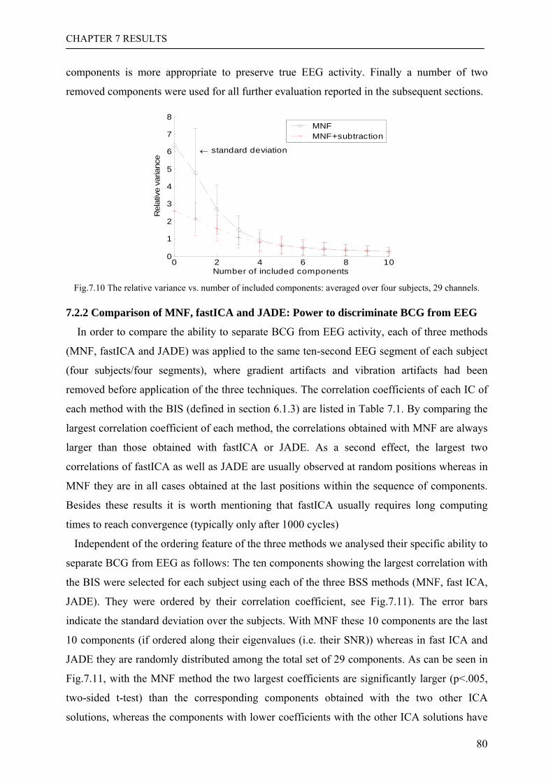
CHAPTER 7 RESULTS
80
components is more appropriate to preserve true EEG activity. Finally a number of two
removed components were used for all further evaluation reported in the subsequent sections.
0 2 4 6 8 100
1
2
3
4
5
6
7
8
← standard deviation
Number of included components
Rel
ativ
e va
rianc
e
MNFMNF+subtraction
Fig.7.10 The relative variance vs. number of included components: averaged over four subjects, 29 channels.
7.2.2 Comparison of MNF, fastICA and JADE: Power to discriminate BCG from EEG
In order to compare the ability to separate BCG from EEG activity, each of three methods
(MNF, fastICA and JADE) was applied to the same ten-second EEG segment of each subject
(four subjects/four segments), where gradient artifacts and vibration artifacts had been
removed before application of the three techniques. The correlation coefficients of each IC of
each method with the BIS (defined in section 6.1.3) are listed in Table 7.1. By comparing the
largest correlation coefficient of each method, the correlations obtained with MNF are always
larger than those obtained with fastICA or JADE. As a second effect, the largest two
correlations of fastICA as well as JADE are usually observed at random positions whereas in
MNF they are in all cases obtained at the last positions within the sequence of components.
Besides these results it is worth mentioning that fastICA usually requires long computing
times to reach convergence (typically only after 1000 cycles)
Independent of the ordering feature of the three methods we analysed their specific ability to
separate BCG from EEG as follows: The ten components showing the largest correlation with
the BIS were selected for each subject using each of the three BSS methods (MNF, fast ICA,
JADE). They were ordered by their correlation coefficient, see Fig.7.11). The error bars
indicate the standard deviation over the subjects. With MNF these 10 components are the last
10 components (if ordered along their eigenvalues (i.e. their SNR)) whereas in fast ICA and
JADE they are randomly distributed among the total set of 29 components. As can be seen in
Fig.7.11, with the MNF method the two largest coefficients are significantly larger (p<.005,
two-sided t-test) than the corresponding components obtained with the two other ICA
solutions, whereas the components with lower coefficients with the other ICA solutions have
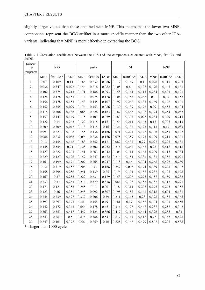
CHAPTER 7 RESULTS
81
slightly larger values than those obtained with MNF. This means that the lower two MNF-
components represent the BCG artifact in a more specific manner than the two other ICA-
variants, indicating that MNF is more effective in extracting the BCG.
Table 7.1 Correlation coefficients between the BIS and the components calculated with MNF, fastICA and JADE.
Number Of
component fv95
pn48
lr64
be98
MNF fastICA* JADE MNF fastICA JADE MNF fastICA* JADE MNF fastICA* JADE1 0,07 0,169 0,11 0,166 0,232 0,066 0,117 0,169 0,1 0,096 0,313 0,2052 0,036 0,347 0,092 0,144 0,216 0,082 0,105 0,64 0,128 0,176 0,147 0,1813 0,102 0,375 0,213 0,171 0,186 0,093 0,158 0,144 0,113 0,234 0,401 0,1214 0,124 0,178 0,153 0,114 0,075 0,128 0,106 0,183 0,268 0,2 0,37 0,1575 0,156 0,178 0,153 0,143 0,145 0,107 0,197 0,242 0,133 0,169 0,196 0,1016 0,152 0,355 0,099 0,174 0,453 0,086 0,139 0,139 0,172 0,09 0,455 0,1047 0,115 0,306 0,136 0,068 0,226 0,163 0,187 0,466 0,108 0,194 0,254 0,0828 0,157 0,447 0,149 0,115 0,107 0,259 0,183 0,307 0,098 0,234 0,329 0,2159 0,122 0,14 0,263 0,129 0,415 0,151 0,154 0,214 0,163 0,13 0,705 0,113
10 0,209 0,309 0,047 0,113 0,115 0,16 0,124 0,132 0,123 0,113 0,17 0,08311 0,091 0,227 0,308 0,155 0,136 0,166 0,071 0,221 0,148 0,106 0,253 0,12212 0,086 0,232 0,088 0,09 0,236 0,156 0,075 0,359 0,173 0,129 0,211 0,30113 0,13 0,155 0,148 0,183 0,352 0,171 0,082 0,437 0,27 0,097 0,297 0,13114 0,148 0,555 0,21 0,128 0,302 0,252 0,216 0,262 0,167 0,23 0,418 0,11815 0,127 0,222 0,203 0,141 0,263 0,242 0,104 0,114 0,163 0,229 0,115 0,33416 0,229 0,127 0,126 0,157 0,247 0,472 0,214 0,154 0,331 0,131 0,356 0,09117 0,161 0,199 0,171 0,207 0,265 0,247 0,118 0,16 0,304 0,268 0,596 0,23918 0,12 0,319 0,157 0,206 0,33 0,168 0,257 0,098 0,174 0,339 0,223 0,30219 0,158 0,395 0,256 0,241 0,139 0,25 0,19 0,194 0,186 0,232 0,127 0,19820 0,167 0,37 0,255 0,222 0,631 0,179 0,153 0,296 0,275 0,157 0,159 0,23221 0,233 0,37 0,263 0,214 0,379 0,318 0,084 0,198 0,187 0,187 0,312 0,29122 0,171 0,121 0,355 0,245 0,13 0,201 0,18 0,314 0,225 0,295 0,295 0,35723 0,423 0,36 0,351 0,248 0,092 0,307 0,195 0,187 0,141 0,318 0,604 0,13124 0,244 0,239 0,497 0,332 0,206 0,39 0,211 0,345 0,28 0,398 0,157 0,36525 0,597 0,297 0,193 0,41 0,454 0,491 0,181 0,17 0,182 0,124 0,123 0,45626 0,442 0,472 0,343 0,656 0,178 0,451 0,316 0,178 0,447 0,237 0,252 0,34227 0,363 0,353 0,417 0,447 0,124 0,366 0,417 0,117 0,444 0,396 0,255 0,31 28 0,643 0,287 0,5 0,876 0,386 0,547 0,817 0,141 0,418 0,76 0,366 0,42829 0,847 0,161 0,392 0,56 0,259 0,46 0,828 0,146 0,479 0,802 0,227 0,538
* : larger than 1000 cycles
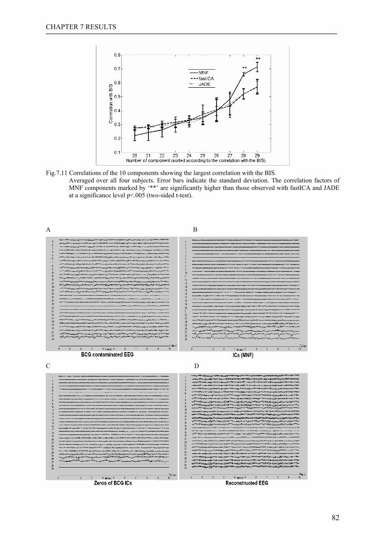
CHAPTER 7 RESULTS
82
Fig.7.11 Correlations of the 10 components showing the largest correlation with the BIS.
Averaged over all four subjects. Error bars indicate the standard deviation. The correlation factors of MNF components marked by ‘**’ are significantly higher than those observed with fastICA and JADE at a significance level p<.005 (two-sided t-test).
A B
C D
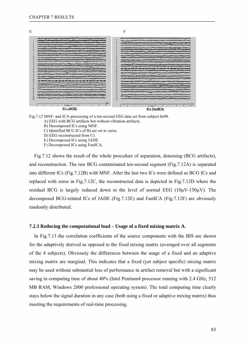
CHAPTER 7 RESULTS
83
E F
Fig.7.12 MNF- and ICA-processing of a ten-second EEG data set from subject be98.
A) EEG with BCG artifacts but without vibration artifacts. B) Decomposed ICs using MNF. C) Identified BCG ICs of B) are set to zeros. D) EEG reconstructed from C). E) Decomposed ICs using JADE. F) Decomposed ICs using FastICA.
Fig.7.12 shows the result of the whole procedure of separation, denoising (BCG artifacts),
and reconstruction. The raw BCG contaminated ten-second segment (Fig.7.12A) is separated
into different ICs (Fig.7.12B) with MNF. After the last two ICs were defined as BCG ICs and
replaced with zeros in Fig.7.12C, the reconstructed data is depicted in Fig.7.12D where the
residual BCG is largely reduced down to the level of normal EEG (10µV-150µV). The
decomposed BCG-related ICs of JADE (Fig.7.12E) and FastICA (Fig.7.12F) are obviously
randomly distributed.
7.2.3 Reducing the computational load – Usage of a fixed mixing matrix A.
In Fig.7.13 the correlation coefficients of the source components with the BIS are shown
for the adaptively derived as opposed to the fixed mixing matrix (averaged over all segments
of the 4 subjects). Obviously the differences between the usage of a fixed and an adaptive
mixing matrix are marginal. This indicates that a fixed (yet subject specific) mixing matrix
may be used without substantial loss of performance in artifact removal but with a significant
saving in computing time of about 40% (Intel Pentium4 processor running with 2.4 GHz, 512
MB RAM, Windows 2000 professional operating system). The total computing time clearly
stays below the signal duration in any case (both using a fixed or adaptive mixing matrix) thus
meeting the requirements of real-time processing.
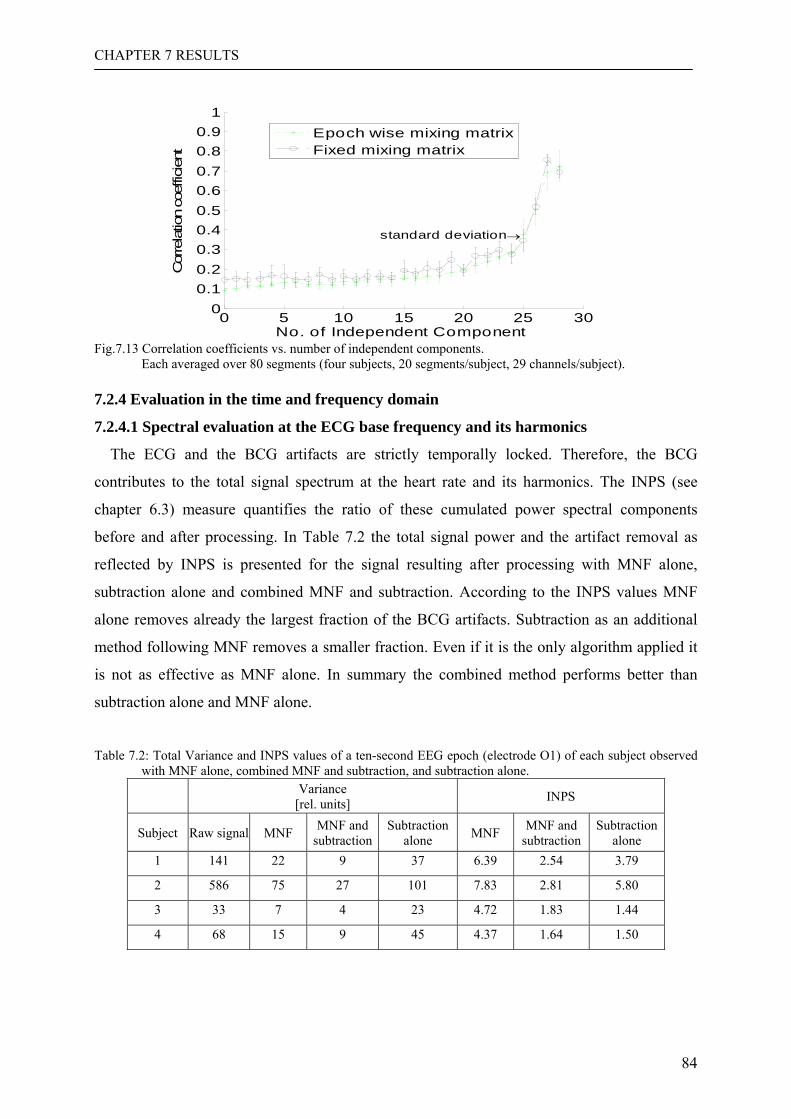
CHAPTER 7 RESULTS
84
0 5 10 15 20 25 300
0.10.20.30.40.50.60.70.80.9
1
standard deviation→
No. of Independent Component
Cor
rela
tion
coef
ficie
nt
Epoch wise mixing matrixFixed mixing matrix
Fig.7.13 Correlation coefficients vs. number of independent components.
Each averaged over 80 segments (four subjects, 20 segments/subject, 29 channels/subject). 7.2.4 Evaluation in the time and frequency domain
7.2.4.1 Spectral evaluation at the ECG base frequency and its harmonics
The ECG and the BCG artifacts are strictly temporally locked. Therefore, the BCG
contributes to the total signal spectrum at the heart rate and its harmonics. The INPS (see
chapter 6.3) measure quantifies the ratio of these cumulated power spectral components
before and after processing. In Table 7.2 the total signal power and the artifact removal as
reflected by INPS is presented for the signal resulting after processing with MNF alone,
subtraction alone and combined MNF and subtraction. According to the INPS values MNF
alone removes already the largest fraction of the BCG artifacts. Subtraction as an additional
method following MNF removes a smaller fraction. Even if it is the only algorithm applied it
is not as effective as MNF alone. In summary the combined method performs better than
subtraction alone and MNF alone.
Table 7.2: Total Variance and INPS values of a ten-second EEG epoch (electrode O1) of each subject observed
with MNF alone, combined MNF and subtraction, and subtraction alone.
Variance
[rel. units] INPS
Subject Raw signal MNF MNF and subtraction
Subtraction alone MNF MNF and
subtraction Subtraction
alone 1 141 22 9 37 6.39 2.54 3.79
2 586 75 27 101 7.83 2.81 5.80
3 33 7 4 23 4.72 1.83 1.44
4 68 15 9 45 4.37 1.64 1.50
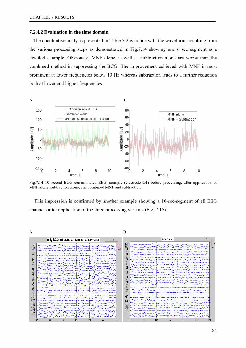
CHAPTER 7 RESULTS
85
7.2.4.2 Evaluation in the time domain
The quantitative analysis presented in Table 7.2 is in line with the waveforms resulting from
the various processing steps as demonstrated in Fig.7.14 showing one 6 sec segment as a
detailed example. Obviously, MNF alone as well as subtraction alone are worse than the
combined method in suppressing the BCG. The improvement achieved with MNF is most
prominent at lower frequencies below 10 Hz whereas subtraction leads to a further reduction
both at lower and higher frequencies.
A B
0 2 4 6 8 10-150
-100
-50
0
50
100
150
time [s]
Am
plitu
de [u
V]
BCG contaminated EEGSubtraction aloneMNF and subtraction combination
0 2 4 6 8 10-80
-60
-40
-20
0
20
40
60
80
time [s]
Am
plitu
de [u
V]
MNF aloneMNF + Subtraction
Fig.7.14 10-second BCG contaminated EEG example (electrode O1) before processing, after application of MNF alone, subtraction alone, and combined MNF and subtraction.
This impression is confirmed by another example showing a 10-sec-segment of all EEG
channels after application of the three processing variants (Fig. 7.15).
A B
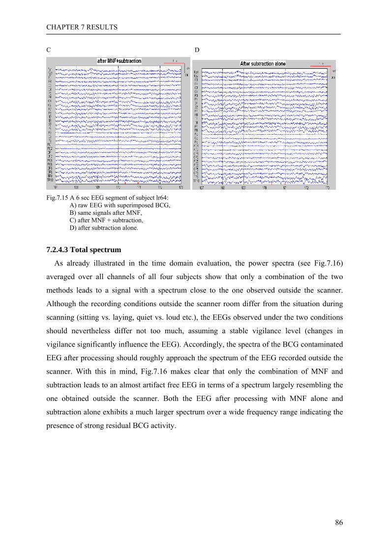
CHAPTER 7 RESULTS
86
C D
Fig.7.15 A 6 sec EEG segment of subject lr64:
A) raw EEG with superimposed BCG, B) same signals after MNF, C) after MNF + subtraction, D) after subtraction alone.
7.2.4.3 Total spectrum
As already illustrated in the time domain evaluation, the power spectra (see Fig.7.16)
averaged over all channels of all four subjects show that only a combination of the two
methods leads to a signal with a spectrum close to the one observed outside the scanner.
Although the recording conditions outside the scanner room differ from the situation during
scanning (sitting vs. laying, quiet vs. loud etc.), the EEGs observed under the two conditions
should nevertheless differ not too much, assuming a stable vigilance level (changes in
vigilance significantly influence the EEG). Accordingly, the spectra of the BCG contaminated
EEG after processing should roughly approach the spectrum of the EEG recorded outside the
scanner. With this in mind, Fig.7.16 makes clear that only the combination of MNF and
subtraction leads to an almost artifact free EEG in terms of a spectrum largely resembling the
one obtained outside the scanner. Both the EEG after processing with MNF alone and
subtraction alone exhibits a much larger spectrum over a wide frequency range indicating the
presence of strong residual BCG activity.
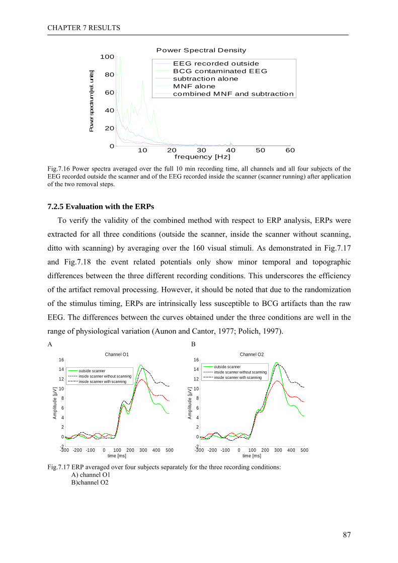
CHAPTER 7 RESULTS
87
10 20 30 40 50 600
20
40
60
80
100
frequency [Hz]
Pow
er s
pect
rum
[rel
. uni
ts]
Power Spectral Density
EEG recorded outsideBCG contaminated EEGsubtraction aloneMNF alonecombined MNF and subtraction
Fig.7.16 Power spectra averaged over the full 10 min recording time, all channels and all four subjects of the EEG recorded outside the scanner and of the EEG recorded inside the scanner (scanner running) after application of the two removal steps.
7.2.5 Evaluation with the ERPs
To verify the validity of the combined method with respect to ERP analysis, ERPs were
extracted for all three conditions (outside the scanner, inside the scanner without scanning,
ditto with scanning) by averaging over the 160 visual stimuli. As demonstrated in Fig.7.17
and Fig.7.18 the event related potentials only show minor temporal and topographic
differences between the three different recording conditions. This underscores the efficiency
of the artifact removal processing. However, it should be noted that due to the randomization
of the stimulus timing, ERPs are intrinsically less susceptible to BCG artifacts than the raw
EEG. The differences between the curves obtained under the three conditions are well in the
range of physiological variation (Aunon and Cantor, 1977; Polich, 1997). A B
-300 -200 -100 0 100 200 300 400 500-2
0
2
4
6
8
10
12
14
16
time [ms]
Am
plitu
de [µ
V]
Channel O1
outside scannerinside scanner without scanninginside scanner with scanning
-300 -200 -100 0 100 200 300 400 500-2
0
2
4
6
8
10
12
14
16
time [ms]
Am
plitu
de [µ
V]
Channel O2
outside scannerinside scanner without scanninginside scanner with scanning
Fig.7.17 ERP averaged over four subjects separately for the three recording conditions:
A) channel O1 B)channel O2
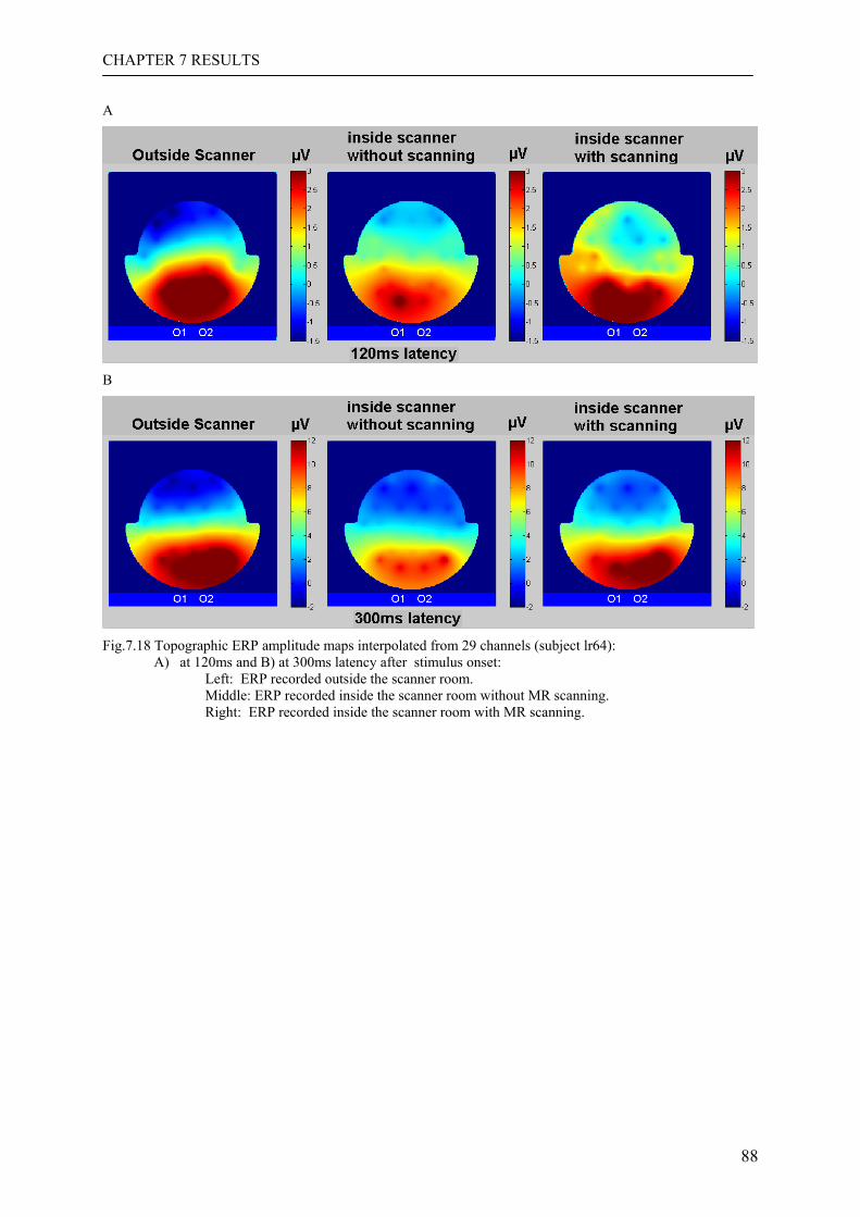
CHAPTER 7 RESULTS
88
A
B
Fig.7.18 Topographic ERP amplitude maps interpolated from 29 channels (subject lr64):
A) at 120ms and B) at 300ms latency after stimulus onset: Left: ERP recorded outside the scanner room. Middle: ERP recorded inside the scanner room without MR scanning. Right: ERP recorded inside the scanner room with MR scanning.
CHAPTER 8 DISCUSSION
89
Chapter 8 Discussion Although there are more and more researches recording EEG and fMRI simultaneously, it
is still a long way for this technique to step into the clinical application because of the main
impediments, namely large gradient artifacts and BCG artifacts superimposed on the normal
EEG.
In physics terms, two principles are responsible for these artifacts: (i) A changing magnetic
field produces an electric field. (ii) The moving closed electrical loop (due to. subject
movement)in the magnetic field induces a current.
The first artifact called ‘gradient artifact’ is caused by the changing magnetic field which is
a consequence of the rapidly switched magnetic field gradients as part of the MR imaging
sequence. These artifacts cannot be avoided because some kind of gradient switching is
needed in any MR imaging sequence.
The second artifact comes from the regular movement of the subject, such as respiration,
and blood flow. All these movements cannot be avoided. Although the breath and heart beat
do not significantly influence the quality of EEG under normal recording conditions, they turn
into a big problem when the EEG is recorded in the magnetic field. This ‘BCG artifact’ is
largely time-locked with the heart beat but slightly varies in its waveform during recording
according to the change in the subject’s position and movement. This limited reproducibility
is the reason for the difficulty of separating BCG artifacts from the EEG background activity
by means of a mere average subtraction technique.
The third artifact named ‘vibration artifact’ is generated due to the cryo-pump of the
scanner. The pump is continuously switched on during scanning in order to avoid overheating
which can lead to a dangerous situation and to a termination of the scanning. The mechanism
leading to a transfer of the pump’s vibration to the EEG artifact (mechanical movement?
Direct electrical coupling?) is not known, but the causal relation is obvious given that the
vibration artifact does not occur if the pump is switched off. It is also worth mentioning that
the artifact amplitude was clearly lower in another MR scanner with lower magnetic field
strength of 1.5 Tesla (GE Signa LX).
8.1 Gradient artifacts
Since the first subtraction method (Allen et al., 2000) appeared, many other methods
(Negishi et al., 2004; Srivastava et al., 2005; Wan et al., 2006) have already been developed.
Becker(2005) has proposed an approach based on the normal subtraction method to remove
CHAPTER 8 DISCUSSION
90
gradient artifacts with a moving weighted window. Unfortunately, these methods could not
avoid the residual gradient artifacts although adaptive noise cancellation (ANC) (Allen et al.,
2000), lowpass filter (Becker et al., 2005) and PCA (Niazy et al., 2005; Schmid et al., 2006)
have worked on reduction of residual gradient artifacts.
One purpose of the new gradient artifacts removing method presented here was to
minimize the residual gradient artifacts by optimizing the subtraction with respect to changes
in the artifact template (Becker et al., 2005 and Herrmann and Debener, 2008) that may occur
due to both non perfect technical stability of the EEG-MR-setting and subjects’ head
movements. Based on Becker’s MAS method, the MAMAS approach improved the
performance of artifact reduction by monitoring the change of electrodes position which
causes the gradient artifacts not to be equal from slice to slice. Besides this effect the
asynchronous timing of the EEG and MR measurement adds to these variations. Furthermore,
tiny long term trends were observed in the artifact waveforms. For a precise analysis of the
character and strength of these variations we conducted phantom measurements in order to
extract the pure artifact waveform without any subject related variability. In these
measurements a watermelon served as a phantom with the same type and number of
electrodes as used for the human measurements. The four different mechanically fixed
orientations lead to four different orientations of the electric loops (consisting of the water
melon surface, the electrodes and the cables) with respect to the gradient magnetic field. In
order to simulate a kind of worst case scenario the watermelon was rotated by two degrees per
step which is certainly at the upper limit of realistic movements. The amplitude differences
between the artifact-templates observed at different orientations were surprisingly high and
reached up to 10% of the absolute artifact amplitude thus underpinning the need for taking
these movements into account. However, even more surprising the shape of the artifact
template changed over short periods of only a few seconds although staying clearly below the
movement related fluctuations. The reported result demonstrates that gradient artifacts are
different from electrode positions and time to time. The underlying technical mechanisms
remain unclear. One may speculate if the warming of the gradient coils leads to very small
changes in the magnetic field giving rise to tiny yet not negligible variations of the artifact
shape. This observation explains the fact that among the evaluated weighting functions the
efficiency in removing the artifact was most pronounced in the Becker version which has the
strongest focus on those epochs positioned closest to the artifact under consideration. In
general two gradient artifacts are similar (yet still slightly varying) within short intervals but
are more and more different with increasing temporal distance. In summary, the gradient
CHAPTER 8 DISCUSSION
91
artifact’s waveform is not constant due to the following reasons: (i) Subject movement due to
the heart beat, (ii) involuntary subject movement independent of the heart beat and (iii) a non
systematic long term trend which of the reason cannot be identified. Especially the movement
related fluctuations of the artifact waveform comes up to 10 % of the total amplitude and must
therefore be included in the algorithm estimating a proper artifact template to be subtracted.
The aim of monitoring the head motion was to decrease the influence of motion on the
gradient artifact removal. By modification of an existing eye-tracking system (Kanowski et
al., 2007) a video based real time monitoring system was developed that constantly traces one
fixed position of the subject’s forehead with a 40 ms temporal resolution. However, since this
device is not available in other MR labs it was only used to (i) test the – later used for
monitoring – SPM realignment tool and (ii) to identify the reason for large residual artifacts
occurring in case of very brief movements which cannot be detected by the SPM realignment
routine. Compared to this high resolution monitor the temporal resolution of the movement
information provided by the SPM-program is worse (half of TR (usually 1000ms)).
Nevertheless this way of movement tracking was preferred to make the method usable for any
MR lab having access to SPM. In general, head movements play a critical role especially in
long lasting (for instance 30 min and more) fMRI experiments. In particular, strong
movements can often not be avoided in patient measurements. Therefore, clinical EEG-fMRI-
measurements will probably benefit most from the improvement achieved with our modified
method. With respect to EEG-guided MR imaging (for instance spike triggered fMRI in
epileptic patients) a real time artifact removal is required. The algorithm in its current version
is non causal and thus not suitable for this purpose. However, in case of not too fast
movements a non causal variant should be sufficient that relies on past epochs only. This
assumption is supported by the observation that the performance of the algorithm in its
current version with the position vector being temporally assigned to the center of the current
half volume does not change if the same information is assigned to the end of the same half
volume. As part of the so called real time movement correction most MR scanners
continuously monitor head movements similar to the SPM-method and thus provide the
position information needed for the artifact removal. Furthermore, a direct head movement
monitor with a much better temporal precision was recently proposed by an external optical
motion tracking (Speck et al., 2006). This device could be used for an improved real-time
movement corrected subtraction algorithm.
Besides the head motion, another important factor influencing the artifact removal is the
asynchrony between the EEG sampling and the fMRI timing. To cope with this effect, various
CHAPTER 8 DISCUSSION
92
methods have been proposed which improve the alignment of the gradient template’s slopes
and peaks by a temporal adjustment of the sampling times by upsampling with different fixed
sampling rates like 50KHz (Becker et al., 2005), 100KHz (Allen et al., 2000) and 20KHz
(Niazy et al., 2005). However, according to the present analysis a much higher rate of about 5
MHz would be needed to keep the residual error below the noise floor due to an imperfect
match. The resampling avoids this extreme boost of data and the related computational load
by replacing the fixed high sampling rate by a temporally adaptive low sampling rate. The
cubic spline interpolation used to calculate the new virtual samples is in this context superior
to sinc interpolation and frequency domain’s interpolation because both create ripple
phenomena at the margins of a signal segment. Cubic splines also outperform linear
interpolation regarding the reconstruction accuracy. The individual resampling with a
temporal resolution of 0.1 us is capable of tracking even a tiny jitter of +/- 0.0025 ms which
was observed in the slice repetition rate of the MR scanner (see below, next paragraph).
Although resampling saves a lot of computation time compared to the upsampling it is still
numerically demanding. To reduce the computational load one could in principle reduce the
signal bandwidth by means of a digital low pass filter and subsequently decimate the
sampling rate before any artifact removal processing. However, the goal of this work is to
optimize the artifact removal algorithm keeping the original bandwidth and sampling rate.
Recently, Goncalves et al. (2007a,b) presented an alternative approach to avoid any mismatch
between the sampling grid applied to the different artifact epochs: Before any processing they
precisely determined the exact inter-slice interval (ISI) in terms of the EEG sampling interval.
From this they calculate the number of samples per slice plus a fraction of the EEG sampling
interval defining the difference between the exact ISI and the nearest integer number of EEG
samples. As shown by these authors, this approach (which largely resembles the electronic
locking between the clocks of the MR- and the EEG-device presented recently by a
commercial supplier) leads to a perfect temporal match of the samples representing the
artifact epochs. However, this only works under the assumption of a perfectly stable ISI. In
our fMRI experiments we observed a spread of about 5 usec in the ISIs observed in the slice
sequence (by determining the slope onset after upsampling by means of interpolation beyond
1 MHz) which is clearly more than the critical threshold determined for our resampling
scheme.
The onsets of gradient artifacts could be easily determined during the trigger supplied by
many MR scanners. However, these triggers are not available in all scanners. Therefore it is
preferable to have a method not depending on this information. An easy solution to this
CHAPTER 8 DISCUSSION
93
problem is available by implementing a threshold comparator detecting the large peak to peak
amplitudes within a gradient artifact period. In practice both methods are comparable both in
temporal precision and computational effort.
The SPM based movement monitor allows to class each epoch into one of several position
levels which is the base for estimating an individual artifact template for each artifact to be
removed. The template is averaged over a limited number of the same level’s epochs within a
restricted period (the moving average window extending over a maximum of 8 sec) to
eliminate the scanner’s systematic long term trends affecting the artifact template. This
limited number of epochs in the vicinity of the actual artifact conflicts with the requirement of
sufficiently large number of epochs needed to keep the residual EEG of the averaged template
below the noise level. As shown by the analysis of EEG signals recorded outside the scanner
and taking into account the phantom related stability measurements, this constraint is clearly
met by the Becker window. In further tests, we observed in cases of no or only mild
movement that even an average over only 10 epochs achieves an artifact reduction that is
comparable (both by eyes and by spectral measures) to the original algorithm. However, the
potential distortion of the ongoing background EEG due to persisting residual EEG carried by
the artifact template cannot be controlled under this condition.
In case of brief strong movements there are not enough artifact epochs available to extract
the reference template because (i) the number of artifacts in the same level would be too small
in the restricted period (even if the brief movement could be precisely traced with a high
resolution movement monitor) and (ii) each artifact has its own shape and is less suitable for
the subtraction process. Therefore after the usual template subtraction a substantial residual
artifact remains to be removed by an alternative approach. This special postprocessing step
was realized in terms of a second subtraction technique where the template is extracted by
averaging over channels rather than over time. Thereby a clear reduction of the artifact
amplitude is achieved which is sufficient for a coarse visual EEG evaluation. However, the
remaining artifact residuum is still larger as compared to signal periods without strong
movement. Since these special cases occur only rarely (typically in 2% of all epochs, in some
subjects not at all) and each time with a different shape a more efficient way of removal
seems hardly feasible.
The remaining residual gradient artifact is to about 50% restricted to frequencies beyond
100 Hz which can be suppressed by appropriate low pass filters without affecting the clinical
relevant EEG frequency bands including the Gamma band. One can only speculate about the
reason for the non perfect removal at all. Given the discrepancy between the almost perfect
CHAPTER 8 DISCUSSION
94
resampling shown in the simulation and the residual amplitudes even after precisely
resampling the real artifact one might speculate if tiny noise or a limited reproducibility of the
gradient’s time course contributes to the high frequency residuals which are most pronounced
close to the steep slopes of the gradient. Second, very mild head movements which cannot be
detected by the movement monitor may nevertheless cause a slight deformation of the artifact
which is not captured by the average template used for subtraction. Finally, although we did
not observe severe differences in the removal performance for different interpolation schemes
including a sinc-interpolation, we cannot exclude that the interpolation algorithm introduces
errors around the peak of the real gradient since the true gradient shape is not known.
Looking at the Gamma-EEG frequency band (i.e. beyond about 30 Hz) the question arises
to what extent EEG activity at these frequencies is suitable for a valid quantitative analysis.
Given that the artifacts activity (and thus the residual activity as well) is stable over some
interval the residuum might be assumed to be stable as well thus adding a constant term to the
total band power. If this stability cannot be assumed, only the spectral components between
the harmonics of the gradient repetition rate should be included in the analysis. But even then
the validity of the results would benefit from the improved removal algorithm because the
lower residual harmonics lead to a lower spread of spectral power.
Given the successful application of ICA based methods to the removal of other EEG
artifact types like for instance electrooculogram (EOG) or electrocardiogram (ECG) (Mantini
et al., 2007; Tong et al., 2001) the question arises if blind separation methods could replace
the subtraction method to remove gradient artifacts. We tried this approach but found that due
to the huge artifact-to-signal ratio a large number of the independent components is affected
by the dominant artifact, many of which also carrying significant EEG activity (Mantini et al.,
2007). Consequently, all these components need to be discarded which leads to a loss of EEG
activity at the same time. Alternatively, several groups (Niazy et al., 2005; Schmid et al.,
2006; Mantini et al.,2007) have applied ICA or PCA to reduce residual artifacts after
application of the subtraction method. However, all these methods need to determine the
number of components to include in the artifact processing. While this task is well suitable for
an interactive procedure it is less suitable for a fully automatic processing. Therefore, we
renounced using this method especially since we observed only tiny improvements in our data
after an interactive trial application of fastICA (Hyvaerinen, 1999) as a postprocessing tool.
CHAPTER 8 DISCUSSION
95
8.2 Vibration artifacts
This type of artifact is caused by the periodic vibration of the vacuum pump of the MR
scanner (‘vibration artifact’) that was observed not only in the 3T-MR device (siemens) but -
to a lesser extent - also in the 1.5T-MR (GE).Due to the mechanical vibrations induced by the
cold head of the magnet cooling system of the MRI scanner (Briselli et al., 2006), it exists
only if the recording is conducted inside the scanner. The vibration artifacts could be
completely suppressed with a simple bandstop filter because of its frequencies being restricted
to (but slightly fluctuating) between about 40Hz and 50 Hz. Besides improving the visual
quality of the EEG, the suppression of vibration artifacts is helpful for the separation of BCG
artifacts, because the vibration bursts to some extent lead to distortions of the MNF
components causing a less efficient separation of BCG and EEG. Of course, the selective
suppression of the range around the frequency interval 40…50 Hz interferes with a potential
analysis of the Gamma frequency band. However, frequencies below 40 Hz and beyond 50
Hz (each minus or plus the slop bandwidth) are preserved. The processing sequence, i.e. first
gradient artifact removal and then vibration suppression vs. the inverse order, has no
influence on the artifact removal performance.
8.3 BCG artifacts
Due to the fact that BCG artifacts largely depending on the heart beat and the blood flow
(which are not stable for physiological reasons), only parts of BCG artifacts can be eliminated
by subtracting an average template derived from the ongoing EEG. The applications of BSS
methods such as PCA and ICA have been proposed by others (Srivastava et al., 2005; Briselli
E et al., 2006; Nakamura et al., 2006; Mantini et al., 2007) to remove BCG artifacts. In the
meantime, ICA is a kind of gold standard of EEG artifact removal including BCG removal.
Comparing MNF with ICA variants such as fastICA and JADE, the main difference relates to
theoptimization criterion guiding the decomposition into orthogonal or independent
components. PCA derives uncorrelated variables by a linear transform that is guided by the
criterion of maximizing the variance of the resulting components. ICA assumes statistically
independent components and maximizes the non-gaussianity according to various criteria like
maximization of kurtosis, negentropy or mutual information. MNF differs from these
approaches by directly incorporating the concept of noise being superimposed on a signal as
part of its optimization criterion, which is defined as SNR. As has been shown as part of the
present development, MNF is superior to ICA techniques in its ability to separate BCG
artifacts from true EEG (Table 7.1).
CHAPTER 8 DISCUSSION
96
One considerable advantage of MNF is its low computational demand. A practical
evaluation of this issue included the decomposition of a 10 sec 29 channel EEG epoch with
fastICA, JADE and MNF. It turned out that fastICA is quite slow (about 10 minutes), JADE
is a bit faster (< 4 minutes) and MNF is the fastest (about half a second). Replacing the
adaptively calculated mixing matrix by a fixed – yet subject specific – matrix further speeds
up the algorithm by up to 32% after taking account of the matrix multiplication operations of
EEG data, which occupy the most of computational time due to the fast computation of MNF.
The second big advantage of MNF in the context of BCG removal is the intrinsic ordering
of the ICs according to their SNR values. The components ordering of both fastICA and
JADE are random with respect to this measure. As a consequence, only MNF allows for an
easy fully automatic procedure of selecting (and subsequently discarding) components
carrying artifact activity. In contrast, the two ICA techniques require additional complex
detection algorithms and in some algorithms also the additional recording of an ECG signal to
determine the BCG specific components (see for instance Tong et al., 2001; Be´nar et al.,
2003, Joyce et al., 2004, Srivastava et al., 2005; Briselli et al., 2006).
According to the basic signal and noise concept of MNF, selecting the last few (or first few,
depending on the direction of ordering) components as the ones to be discarded is successful
as long as the BCG is the largest artifact occurring in the EEG. This is almost always that the
BCG amplitudes are much larger than any other artifact. However, theoretically this
procedure might be less effective, in cases where the BCG is accompanied by other
continuous strong artifacts like for instance constant EOG and/or EMG. However, even then
(i) the suppression of the last/first components will lead to a reduction of these artifacts in
general and (ii) the subsequent subtraction will still remove most of the BCG. Ultimately, in
an extreme case where other but BCG artifacts are clearly dominant, the EEG would hardly
be evaluated since its quality is absolutely insufficient irrespectively of the BCH artifacts.
This situation was never encountered in any of the recordings presented here.
The decomposed ICs of MNF are only approximately independent because MNF tries to
minimize the correlation between components which not necessarily leads to statistical
independence between these components. Second, the BCG artifact presumably is not
completely independent from the EEG (this relation cannot be tested because the pure BCG
cannot be observed). As a consequence, the BCG artifacts are distributed over more than just
one MNF component. Thus setting the number of BCG ICs becomes a dilemma regarding the
balance of removed BCG artifacts and suppressed true EEG. In the EEG examples of this
work, the last four ICs contain the most parts of BCG artifacts, but a predefined number, two
CHAPTER 8 DISCUSSION
97
components to discard, is a conservative strategy in order to keep as much true EEG as
possible. This strategy necessarily leads to a non negligible amount of remaining residual
BCG activity in many cases. Therefore, the subsequent subtraction method is necessary to
further reduce these residuals.
The subtraction method used here is based on the normal subtraction method as introduced
by Allen et al. (1998) but was modified by the introduction of a moving average template
which is capable of tracking changes in the shape of the residual BCG. Due to the fact that
BCG artifacts significantly vary over time for various reasons this adaptive procedure is more
effective with respect to the ultimate residual BCG persisting after these two processing steps.
The combined MNF-subtraction method removes substantially more of the BCG artifact than
both of the two methods alone indicating that obviously MNF and subtraction extract
different parts of the artifact complex. This conclusion is further supported by the fact that the
power spectra of the signals obtained after the two individual processing steps deviate in
different ways from the spectrum derived from the final EEG resulting after the two
processing steps. Furthermore, the similarity between this final spectrum and the one obtained
from the EEG recorded outside the scanner indicates that the BCG has been successfully
removed without suppressing substantial parts of the underlying EEG. The minor differences
seen between 2…10 Hz may be attributed to the very different environmental conditions
during recording, which may well lead to different degrees of vigilance. In addition, the
acoustic background noise in the scanner could have physiologically interfered with the
ongoing EEG.
The visual perception ERP-experiment demonstrates the validity of the combined method in
the caseof temporal and spatial ERP analysis. The visual ERPs calculated under the three
conditions (outside the MR room, inside the MR room without scanning and inside the MR
room with scanning) are comparable very much and thus proof that the removal of the
gradient and BCG artifacts does not affect the ERP results.
CHAPTER 9 SUMMARY
98
Chapter 9 Summary The simultaneous recording of EEG and fMRI is a promising tool in neuroimaging
research. However, three types of large artifacts dominate and completely obscure the EEG if
recorded inside the scanner: (i) artifacts related to the switched MR gradients with steep
slopes and extremely large amplitudes of about more than hundred times normal EEG
amplitudes, (ii) vibration artifacts showing periodic burst around 40...50 Hz originating at the
vaccum pump of the MR scanner and (iii) ballistocardiogram (BCG) artifacts with lower
amplitudes and primarily low frequency components caused by heart rate induced tiny body
movements.
With the goal of improving current gradient artifact removal techniques, a new method is
presented called movement adapted moving average subtraction (MAMAS). It integrates an
adaptive resampling technique, a gradient artifact template extraction algorithm guided by a
head motion monitor and a special postprocessing tool to reduce irregular artifacts. It
suppresses the residual gradient artifacts down to a level clearly below usual EEG amplitudes
of about 10-100 µV. The resampling is comparable to an upsampling of the signal to an
extremely high sampling but it avoids the boost of data and computational load. It greatly
suppresses the error resulting from the asynchronous sampling of the EEG and the MR. Head
motion monitoring was accomplished by using the SPM movement correction routine.
Although the temporal resolution of SPM tracing is limited by half the TR-time of the
scanning sequence, it is sufficient to guide the averaging algorithm to include only those
epochs recorded at the same head position as the artifact to be removed. This technique
reduces the residual artifact activity by about 50% compared to the moving average
subtraction technique (MAS) as proposed by other groups. However, brief sub-second
motions are not correctly represented by the SPM monitoring data thus leading to a large
residual artifact after MAMAS processing. For these cases an additional special
postprocessing algorithm was developed that virtually replaced the averaging of artifacts over
time by averaging over channels to extract a proper template. Vibration artifacts can be easily
removed by a 40-50 Hz bandstop filter, however at the cost of a loss of true EEG in the same
frequency band. The only way of avoiding this artifact is halting the pump during EEG-MR-
measurements.
Several ICA based approaches have been proposed to remove BCG artifacts. In the present
work another blind source separation technique called maximum noise fraction (MNF) has
been applied to further improve the separation between BCG artifact and EEG, substantially
CHAPTER 9 SUMMARY
99
reduce the computational demands and finally provide a set of components which are sorted
along their signal to noise ratio thereby facilitating the development of a fully automatic
removal procedure. After application of the MNF algorithm the artifact reduction is
completed by appending an additional average subtraction algorithm which removes some
spurious residuals existing after MNF processing. It is shown that both MNF alone and
subtraction alone are not capable of providing a sufficient reduction of BCG artifact activity.
The comparison of power spectra computed from the artifact reduced EEGs with those
spectra observed in EEGs recorded from the same subjects but outside the scanner room (i.e.
without any MR related artifact) shows only minor differences which are most likely due to
vigilance fluctuations or other physiological fluctuations. This result is confirmed by the
results of ERP measurements conducted under the same conditions. Again there are only
marginal temporal and topographic differences which are in the range of normal physiologic
variations well known in this field of research.
BIBLIOGRAPHY
100
Bibliography
Allen, P.J., Polizzi, G., Krakow, K., Fish, D.R., Lemieux, L., 1998. Identification of EEG
events in the MR scanner: the problem of pulse artifact and a method for its subtraction.
NeuroImage 8 (3), 229–239.
Allen, P.J., Josephs, O., Turner, R., 2000. A method for removing imaging artifact from
continuous EEG recorded during functional MRI. NeuroImage 12 (2), 230– 239.
Anami, K., Mori, T., Tanaka, F., Kawagoe, Y., Okamoto, J., Yarita, M., Ohnishi, T., Yumoto,
M., Matsuda, H., Saitoh, O., 2003. Stepping stone sampling for retrieving artifact-free
electroencephalogram during functional magnetic resonance imaging. NeuroImage 19 (2
Pt. 1), 281–295.
Anderle, M. G., and Kirby, M. J., 2001. An application of the maximum noise fraction
method to filtering noisy time series, in Proc. 5th International Conference on
Mathematics in Signal Processing, University of Warwick, Coventry, UK.
Aunon JI, Cantor FK., 1977. VEP and AEP variability: interlaboratory vs. intralaboratory and
intersession vs. intrasession variability. Electroencephalogr Clin Neurophysiol., 42(5),
705-708
Barbati, G., Porcaro,C., Zappasodi, F., Rossini, P.M., Tecchio, F., 2004. Optimization of an
independent component analysis approach for artifact identification and removal in
magnetoencephalographic signals. Clinical Neurophysiology 115 (5), 1220-1232.
Becker, R., Ritter, P., Moosmann, M., Villringer A., 2005. Visual Evoked Potentials
Recovered From fMRI Scan Periods. Human Brain Mapping 26, 221–230.
Bell, A.J., Sejnowski, T.J., 1995. An information-maximization approach to blind separation
and blind deconvolution. Neural Computation 7, 1129-1159.
Be´nar, C., Aghakhani, Y., Wang, Y., Izenberg, A., Al-Asmi, A., Dubeau, F.,Gotman, J.,
2003. Quality of EEG in simultaneous EEG–fMRI for epilepsy. Clin. Neurophysiol. 114
(3), 569– 580.
Blaschke, T., Wiskott, L., 2004, CuBICA: Independent Component Analysis by Simultaneous
Third- and Fourth-Order Cumulant Diagonalization. IEEE Transactions on Signal
Processing, 52 (5), 1250-1256.
Bonmassar, G., Anami, K., Ives, J., Belliveau, J.W., 1999. Visual evoked potential (VEP)
measured by simultaneous 64-channel EEG and 3T fMRI. NeuroReport 10 (9), 1893–
1897.
BIBLIOGRAPHY
101
Bonmassar, G., Purdon, P.L., Jaaskelainen, I.P., Chiappa, K., Solo, V., Brown, E.N.,
Belliveau, J.W., 2002. Motion and ballistocardiogram artifact removal for interleaved
recording of EEG and EPs during MRI. NeuroImage 16 (4), 1127–1141.
Briselli, E., Garreffa, G., Bianchi, L., Bianciardi, M., Macaluso, E., Abbafati, M., Marciani,
M.G., Maraviglia, B., 2006. An independent component analysis-based approach on
ballistocardiogram artifact removing. Magnetic Resonance Imaging 24, 393-400.
Comon, P., 1994. Independent Component Analysis, a new concept? Signal Processing,
Elsevier, vol.36, no. 3, pp. 287-314, special issue on Higher-Order Statistics.
Cardoso, J.-F., 1989. Source separation using higher order moments. In Proc. ICASSP, pages
2109-2112.
Cardoso, J.F., 1998. Blind signal separation: statistical principles. Proceedings of the IEEE. 9,
2009-2025.
Cardoso, J.-F., 1999. High-order contrasts for independent component analysis. Neural
Computation, vol. 11, no. 1, 157-192.
Cohen, M. S., Goldman, R. I., Stern, J., and Engel, Jr. J., 2001. Simultaneous EEG and fMRI
made easy. NeuroImage, 13 (6 Supp.1), S6.
Comon, P., 1994. Independent Component Analysis, a new concept? Signal Processing,
Elsevier, vol.36, no. 3, pp. 287-314, special issue on Higher-Order Statistics.
Chatrian, G.E., Lettich, E., Nelson, P.L., 1985. Ten percent electrode system for topographic
studies of spontaneous and evoked EEG activity. Am. J. EEG Technol. 25, 83–92.
Damadian R, Goldsmith M, Minkoff L, 1977. NMR in cancer: XVI. FONAR image of the
live human body. Physiol Chem Phys. 9 (1), 97-100, 108.
Debener, S., Strobel,A., Sorger,B., Peters, J., Kranczioch, C., Goebel, R., 2007. Improved
quality of auditory event-related potentials recorded simultaneously with 3-T fMRI:
Removal of the ballistocardiogram artifact. NeuroImage 34 (2), 587-597
De Lathauwer, L., De Moor, B., Vandewalle, J., 2000. An introduction to independent
component analysis. J. Chemometrics, 14, 123-149.
Ernst Niedermeyer, Fernando Lopes da Silva, 1987. Electroencephalography: basic
principles, clinical applications, and related fields (third edition).
Ellingson, M.L., Liebenthal, E., Spanaki, M.V., Prieto, T.E., Binder, J.R., Ropella, K.M.,
2004. Ballistocardiogram artifact reduction in the simultaneous acquisition of auditory
ERPS and fMRI. NeuroImage 22 (4), 1534– 1542.
BIBLIOGRAPHY
102
Felblinger, J., Slotboom, J., Kreis, R., Jung, B., Boesch, C., 1999. Restoration of
electrophysiological signals distorted by inductive effects of magnetic field gradients
during MR sequences. Magn. Reson. Med. 41 (4), 715-721.
Flexer, A. Bauer, H., Pripfl, J., Dorffner, G., 2005. Using ICA for removal of ocular artifacts
in EEG recorded from blind subjects. Neural Netw. 18 (7), 998-1005.
Foucher, J. R., Otzenberger, H., and Gounot, D., 2003. The BOLD response and the gamma
oscillations respond differently than evoked potentials: an interleaved EEG-fMRI study.
BMC neuroscience 4, 22.
Friston KJ, Ashburner J, Frith CD, Poline J-B, Heather JD & Frackowiak RSJ , 1995. Spatial
registration and normalization of images Hum. Brain Map. 2, 165-189.
Garreffa, G., Carni, M., Gualniera, G., Ricci, G.B., Bozzao, L., De Carli, D., Morasso, P.,
Pantano, P., Colonnese, C., Roma, V., Maraviglia, B., 2003. Real-time MR artifacts
filtering during continuous EEG/fMRI acquisition. Magn. Reson. Imaging 21 (10), 1175-
1189.
Goldman, R.I., Stern, J.M., Engel, J., Cohen, M.S., 2000. Acquiring simultaneous EEG and
functional MRI, Clinical Neurophysiology 111, 1974-1980
Goldman, R.I., Stern, J.M., Engel, J., Cohen, M.S., 2002. Simultaneous EEG and FMRI of the
alpha rhythm. NeuroReport 13 (18), 2487-2492.
Goncalves, S.I., Pouwels, P.J., Kuijer, J.P., Heethaar, R.M., de Munck, J.C., 2007a. Artifact
removal in co-registered EEG/fMRI by selective average subtraction. Clin. Neurophysiol.
118 (11), 2437-50.
Goncalves, S.I., Pouwels, P.J., Kuijer, J.P., Heethaar, R.M., de Munck, J.C., 2007b.
Correction for desynchronization of EEG and fMRI clocks through data interpolation
optimizes artifact reduction. Conf. Proc. IEEE Eng. Med. Biol. Soc. 1, 1590-4.
Grassberger P, Hegger R, Kanz H, Schaffrath C, Schreiber T., 1993. On noise reduction
methods for chaotic data. Chaos, 3(2), 127–41.
Green, A. A., Berman, M., Switzer, P., and Craig, M. D., 1988. A transformation for ordering
multispectral data in terms of image quality with implications for noise removal, IEEE
Trans. Geosci. Remote Sensing, vol. 26 (1), 65–74,.
Herault, J. and Jutten, C., 1986. Space or time adaptive signal processing by neural network
models. AIP Conference Proceedings, 151, 206-211.
Herrmann, C.S., Debener, S., 2008. Simultaneous recording of EEG and BOLD responses: A
historical perspective. International Journal of Psychophysiology, 67, 161-168.
BIBLIOGRAPHY
103
Hill, R.A., Chiappa, K.H., Huang-Hellinger, F., Jenkins, B.G., 1995. EEG during MR
imaging: Differentiation of movement artifact from paroxysmal cortical activity.
American Academy of Neurology 45, 1942-1943.
Hoffmann, A., Ja¨ger, L., Warhahn, K.J., Jaschke, M., Noachtar, S., Reiser, M., 2000.
Electroencephalography during functional echo-planar imaging: detection of epileptic
spikes using post-processing methods. Magn. Reson. Med. 44, 791–798.
Huettel, S.A., Song, A.W., McCarthy, G., 2003. Functional Magnetic Resonance Imaging,
Sinauer Associates Inc. Publishers, Sunderland, MA, USA.
Huiskamp, G.J., 2005. Reduction of the Ballistocardiogram artifact in simultaneous EEG-
fMRI using ICA. Conf Proc IEEE Eng Med Biol Soc. 4, 3691-3694.
Hundley, D., Kirby M., Anderle, M.G., 2001. A Solution Procedure for Blind Signal
Separation using the Maximum Noise Fraction Approach: Algorithms and Examples,
Proceedings of the Conference on Independent Component Analysis, San Diego, CA,
337–342.
Hundley, D.R., Kirby, M.J., Anderle, M., 2002. Blind source separation using the maximum
signal fraction approach, Signal Processing 82, 1505-1508.
Huang-Hellinger FR, Breiter HC, McCormack G, Cohen MS, Kwong KK, Sutton JP, Savoy
RL, Weisskoff RM, Davis TL, Baker JR, Belliveau JW, Rosen BR, 1995. Simultaneous
functional magnetic resonance imaging and electrophysiological recording. Hum Brain
Map 3, 13–23.
Hyvaerinen A., 1999 Fast and robust fixed-point algorithms for independent component
analysis. IEEE Trans Neural Netw. 10 (3), 626-634.
Ives, J.R., Warach, S., Schmitt, F., Edelman, R.R., Schomer, D.L., 1993. Monitoring the
patient’s EEG during echo planar MRI. Electroencephalogr. Clin. Neurophysiol. 87, 417-
420.
Jasper, H.H., 1958: The ten-twenty electrode system of the international federation.
Electroencephal. Clin. Neurophysiology, 10, 1426-1437.
Joyce, C.A., Gorodnitsky, I.F., Kutas, M., 2004. Automatic removal of eye movement and
blink artifacts from EEG data using blind component separation. Psychophysiology, 41
(2) 313-325.
Kanowski, M., Rieger, J. W., Noesselt, T., Tempelmann, C., Hinrichs, H., 2007. Endoscopic
eye tracking system for MRI. J. Neurosci. Methods 160 (1), 10-15.
Kim, K.H., Yoon, H.W., Park, H.W., 2004. Improved ballistocardiac artifact removal from
the electroencephalogram recorded in fMRI. J. Neurosci. Methods 135 (1– 2), 193– 203.
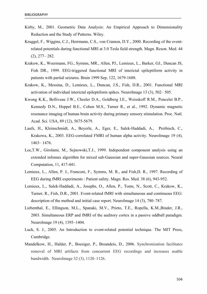
BIBLIOGRAPHY
104
Kirby, M., 2001. Geometric Data Analysis: An Empirical Approach to Dimensionality
Reduction and the Study of Patterns. Wiley.
Kruggel, F., Wiggins, C.J., Herrmann, C.S., von Cramon, D.Y., 2000. Recording of the event-
related potentials during functional MRI at 3.0 Tesla field strength. Magn. Reson. Med. 44
(2), 277– 282.
Krakow, K., Woermann, FG., Symms, MR., Allen, PJ., Lemieux, L., Barker, GJ., Duncan JS,
Fish DR., 1999. EEG-triggered functional MRI of interictal epileptiform activity in
patients with partial seizures. Brain 1999 Sep, 122, 1679-1688.
Krakow, K., Messina, D., Lemieux, L., Duncan, J.S., Fish, D.R., 2001. Functional MRI
activation of individual interictal epileptiform spikes. NeuroImage 13 (3), 502– 505.
Kwong K.K., Belliveau J.W., Chesler D.A., Goldberg I.E., Weisskoff R.M., Poncelet B.P.,
Kennedy D.N., Hoppel B.E., Cohen M.S., Turner R., et al., 1992. Dynamic magnetic
resonance imaging of human brain activity during primary sensory stimulation. Proc. Natl.
Acad. Sci. USA, 89 (12), 5675-5679.
Laufs, H., Kleinschmidt, A., Beyerle, A., Eger, E., Salek-Haddadi, A., Preibisch, C.,
Krakowa, K., 2003. EEG-correlated FMRI of human alpha activity. NeuroImage 19 (4),
1463– 1476.
Lee,T.W., Girolami, M., Sejnowski,T.J., 1999. Independent component analysis using an
extended infomax algorithm for mixed sub-Gaussian and super-Gaussian sources. Neural
Computation, 11, 417-441.
Lemieux, L., Allen, P. J., Franconi, F., Symms, M. R., and Fish,D. R., 1997. Recording of
EEG during fMRI experiments : Patient safety. Magn. Res. Med. 38 (6), 943-952.
Lemieux, L., Salek-Haddadi, A., Josephs, O., Allen, P., Toms, N., Scott, C., Krakow, K.,
Turner, R., Fish, D.R., 2001. Event-related fMRI with simultaneous and continuous EEG:
description of the method and initial case report. NeuroImage 14 (3), 780–787.
Liebenthal, E., Ellingson, M.L., Spanaki, M.V., Prieto, T.E., Ropella, K.M.,Binder, J.R.,
2003. Simultaneous ERP and fMRI of the auditory cortex in a passive oddball paradigm.
NeuroImage 19 (4), 1395–1404.
Luck, S. J., 2005. An Introduction to event-related potential technique. The MIT Press,
Cambridge.
Mandelkow, H., Halder, P., Boesiger, P., Breandeis, D., 2006. Synchronization facilitates
removal of MRI artifacts from concurrent EEG recordings and increases usable
bandwidth. NeuroImage 32 (3), 1120–1126.
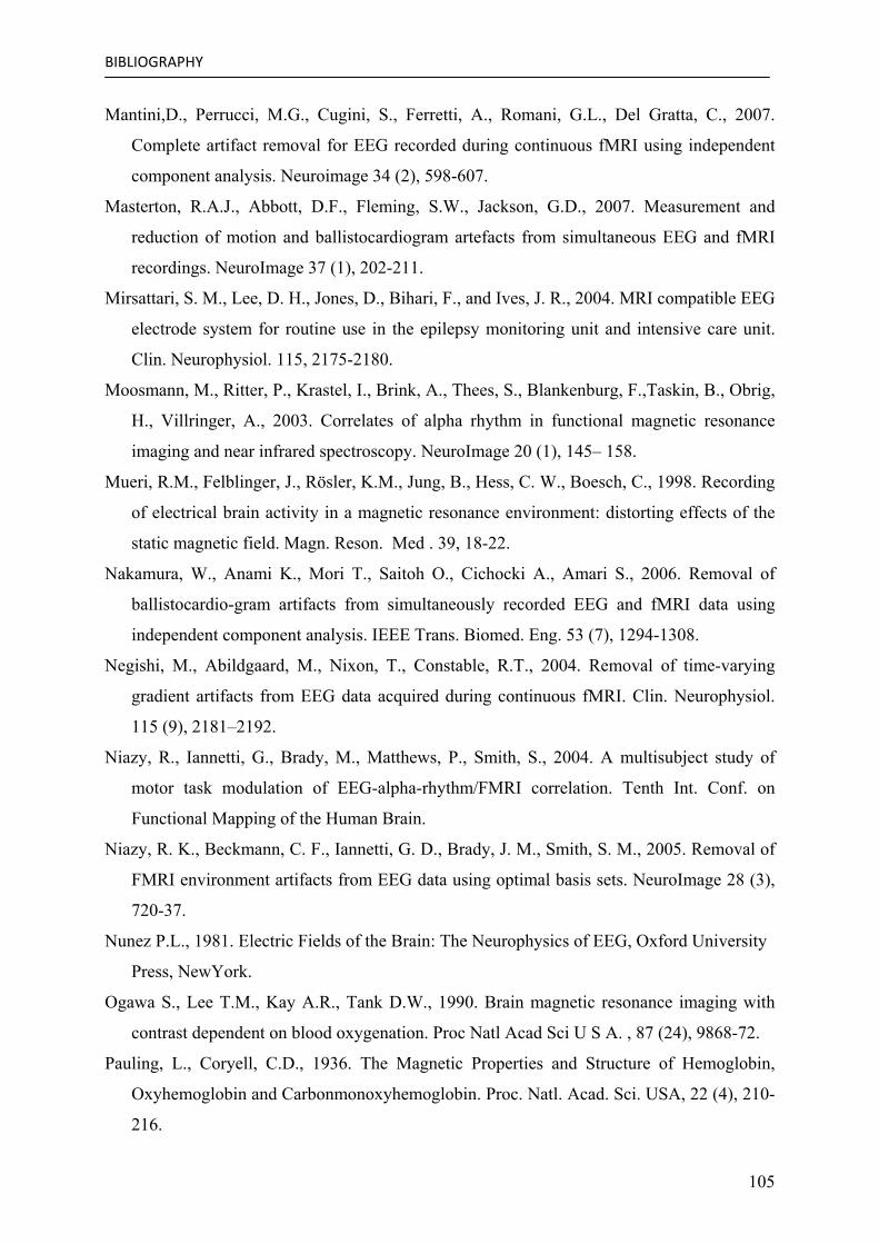
BIBLIOGRAPHY
105
Mantini,D., Perrucci, M.G., Cugini, S., Ferretti, A., Romani, G.L., Del Gratta, C., 2007.
Complete artifact removal for EEG recorded during continuous fMRI using independent
component analysis. Neuroimage 34 (2), 598-607.
Masterton, R.A.J., Abbott, D.F., Fleming, S.W., Jackson, G.D., 2007. Measurement and
reduction of motion and ballistocardiogram artefacts from simultaneous EEG and fMRI
recordings. NeuroImage 37 (1), 202-211.
Mirsattari, S. M., Lee, D. H., Jones, D., Bihari, F., and Ives, J. R., 2004. MRI compatible EEG
electrode system for routine use in the epilepsy monitoring unit and intensive care unit.
Clin. Neurophysiol. 115, 2175-2180.
Moosmann, M., Ritter, P., Krastel, I., Brink, A., Thees, S., Blankenburg, F.,Taskin, B., Obrig,
H., Villringer, A., 2003. Correlates of alpha rhythm in functional magnetic resonance
imaging and near infrared spectroscopy. NeuroImage 20 (1), 145– 158.
Mueri, R.M., Felblinger, J., Rösler, K.M., Jung, B., Hess, C. W., Boesch, C., 1998. Recording
of electrical brain activity in a magnetic resonance environment: distorting effects of the
static magnetic field. Magn. Reson. Med . 39, 18-22.
Nakamura, W., Anami K., Mori T., Saitoh O., Cichocki A., Amari S., 2006. Removal of
ballistocardio-gram artifacts from simultaneously recorded EEG and fMRI data using
independent component analysis. IEEE Trans. Biomed. Eng. 53 (7), 1294-1308.
Negishi, M., Abildgaard, M., Nixon, T., Constable, R.T., 2004. Removal of time-varying
gradient artifacts from EEG data acquired during continuous fMRI. Clin. Neurophysiol.
115 (9), 2181–2192.
Niazy, R., Iannetti, G., Brady, M., Matthews, P., Smith, S., 2004. A multisubject study of
motor task modulation of EEG-alpha-rhythm/FMRI correlation. Tenth Int. Conf. on
Functional Mapping of the Human Brain.
Niazy, R. K., Beckmann, C. F., Iannetti, G. D., Brady, J. M., Smith, S. M., 2005. Removal of
FMRI environment artifacts from EEG data using optimal basis sets. NeuroImage 28 (3),
720-37.
Nunez P.L., 1981. Electric Fields of the Brain: The Neurophysics of EEG, Oxford University
Press, NewYork.
Ogawa S., Lee T.M., Kay A.R., Tank D.W., 1990. Brain magnetic resonance imaging with
contrast dependent on blood oxygenation. Proc Natl Acad Sci U S A. , 87 (24), 9868-72.
Pauling, L., Coryell, C.D., 1936. The Magnetic Properties and Structure of Hemoglobin,
Oxyhemoglobin and Carbonmonoxyhemoglobin. Proc. Natl. Acad. Sci. USA, 22 (4), 210-
216.

BIBLIOGRAPHY
106
Peterson, D.A., Knight, J.N., Kirby, M.J., Anderson, C.W., and Thaut, M.H., 2005. Feature
Selection and Blind Source Separation in an EEG-Based Brain-Computer Interface,
Journal on Applied Signal Processing 19, 3128–3140.
Polich, J., 1997. On the relationship between EEG and P300: individual differences, aging,
and ultradian rhythms. Int J Psychophysiol. 26 (1-3), 299-317.
Salek-Haddadi, A., Lemieux, L., Merschhemke, M., Diehl, b., Allen, P. J., and Fish, D. R.,
2003. EEGquality during simultaneous functional MRI of interictal epileptiform
discharges. Magn. Reson. Imag. 21, 1159-1166.
Schmid, M. C., Oeltermann, A., Juchem, C., Logothetis, N.K., Smirnakis, S. M., 2006.
Simultaneous EEG and fMRI in the macaque monky at 4.7 Tesla. Magnetic Resonance
Imaging 24, 335-342.
Schomer, D.L., Bonmassar, G., Lazeyras, F., Seeck, M., Blum, A., Anami, K., Schwartz, D.,
Belliveau, J. W., and Ives, J., 2000. EEG-Linked Functional Magnetic Resonance Imaging
in Epilepsy and Cognitive Neurophysiology. J. Clin. Neurophysiol. 17, 43-58.
Seeck, M., Michel, C.M., Spinelli, L., Lazeyras, F., 2001. EEG mapping and functional MRI
in presurgical epilepsy evaluation. Rev. Neurol. (Paris) 157 (8– 9 Pt. 1), 747– 751.
Sijbers, J., Michiels, I., Verhoye, M., Van Auderkerke, J., Van der Linden, A., and Van Dyck,
D., 1999. Restoration of MR-induced artifacts in simultaneously recorded MR/EEG data.
Magn. Reson. Imag. 17 (9), 1383–1391.
Sijbers, J., Van Audekerke, J., Verhoye, M., Van der Linden, A., Van Dyck, D., 2000.
Reduction of ECG and gradient related artifacts in simultaneously recorded human
EEG/MRI data. Magn. Reson. Imaging 18 (7), 881– 886.
Sommer, M., Meinhardt, J., and Volz, H.P., 2003. Combined Measurement of Event-Related
Potentials(ERPs) and fMRI. Acta Neurobiol. Exp. 63,49-53.
Souloumiac A. and Cardoso J.-F., 1991. Comparaisons de Me´hodes de Se´paration de
Sources, Xlllth Coll.GRETSI, September, 661- 664.
Souloumiac A. and Cardoso J.-F., 1996. Jacobi angles for simultaneous diagonalization.
SIAM J. Matrix Anal. Appl. 17 , 161-164.
Speck, O., Hennig, J., Zaitsev, M., 2006. Prospective real-time slice-by-slice motion
correction for fMRI in freely moving subjects. MAGMA 19( 2), 55-61.
Srivastava, G., Crottaz-Herbette, S., Lau, K.M., Glover, G.H., Menon, V., 2005. ICA-based
procedures for removing ballistocardiogram artifacts from EEG data acquired in the MRI
scanner. NeuroImage 24 (1), 50– 60.
BIBLIOGRAPHY
107
Tong, S., Bezerianos, A., Paul, J., Zhu, Y., Thakor, N., 2001. Removal of ECG interference
from the EEG recordings in small animals using independent component analysis. J.
Neuroscience Methods 108 (1), 11-17.
Vincent, J.L., Larson-Prior, L.J., Zempel, J.M., Snyder, A.Z., 2007. Moving GLM
ballistocardiogram artifact reduction for EEG acquired simultaneously with fMRI.
Clinical Neurophysiology 118, 981-998.
Warach, S., Ives, J.R., Schlaug, G., Patel, m.D., Darby, D.G., Thangaraj, V., Edelman, R. R.,
and Schomer, D. L., 1996. EEG-triggered echo-planar functional MRI in epilepsy.
Neurology 47, 89-93.
Wan, X., Iwata, K., Riera, J., Ozaki, T., Kitamura, M., Kawashima, R., 2006a. Artifact
reduction for EEG/fMRI recording: Nonlinear reduction of ballistocardiogram artifacts.
Clinical Neurophysiology 117 (3), 668–680.
Wan, X., Iwata, K., Riera, J., Kitamura, M., and Kawashima, R., 2006b. Artifact reduction for
simultaneous EEG/fMRI recording: Adaptive FIR reduction of imaging artifacts. Clinical
Neurophysiology 117 (3), 681–692.
Welch, P.D., 1967. The use of fast Fourier transform for the estimation of power spectra: a
method based on time averaging over short, modified periodograms. IEEE Trans. Audio
Electroac. AU 15, 70–73.
Zschocke, S., 2002. Klinische Elektroenzephalographie. Springer.


![NSF Project EEG CIRCUIT DESIGN. Micro-Power EEG Acquisition SoC[10] Electrode circuit EEG sensing Interference](https://img.dokumen.tips/doc/110x75/56649cfb5503460f949ccecd/nsf-project-eeg-circuit-design-micro-power-eeg-acquisition-soc10-electrode.jpg)
![Class-wise Deep Dictionaries for EEG Classificationsalsa.iiitd.edu.in/contents/angshul/2016/PrernaIJCNN2016.pdf · Representation based Classification (SRC) approach [3]; instead](https://img.dokumen.tips/doc/110x75/5eceb805ac8f391609197e65/class-wise-deep-dictionaries-for-eeg-representation-based-classification-src-approach.jpg)