Embed Size (px)
Citation preview
Simultaneous estimation of soil hydraulic and solute transportparameters from transient in®ltration experiments
M. Inoue a, J. �Sim�unek b,*, S. Shiozawa c, J.W. Hopmans d
a Arid Land Research Center, Tottori University, Hamasaka 1390, Tottori 680, Japanb US Salinity Laboratory, USDA-ARS, 450 W. Big Springs Dr., Riverside, CA 92507, USA
c Institute of Agricultural and Forest Engineering, University of Tsukuba, Tsukuba, Japand Hydrology Program, Department LAWR, 123 Veihmeyer Hall, University of California, Davis, CA 95616, USA
Received 6 October 1999; received in revised form 10 February 2000; accepted 11 February 2000
Abstract
Estimation of soil hydraulic and solute transport parameters is important to provide input parameters for numerical models
simulating transient water ¯ow and solute transport in the vadose zone. The Levenberg±Marquardt optimization algorithm in
combination with the HYDRUS-1D numerical code was used to inversely estimate unsaturated soil-hydraulic and solute transport
parameters from transient matric pressure head, apparent electrical conductivity, and e�uent ¯ux measurements. A 30 cm long soil
column with an internal diameter of 5 cm was used for in®ltration experiments in a coarse-textured soil. In®ltration experiments
were carried out with both increasing and decreasing solute concentrations following a sudden increase in the in®ltration rate.
Matric pressure heads and solute concentrations were measured using automated mini-tensiometers and four-electrode sensors,
respectively. The simultaneous estimation results were compared with independently measured soil water retention, unsaturated
hydraulic conductivity, and solute dispersion data obtained from steady-state water ¯ow experiments. The optimized values cor-
responded well with those measured independently within the range of experimental data. The information contained in the ap-
parent electrical conductivity (which integrates information about both water ¯ow and solute transport) proved to be very useful for
the simultaneous estimation of soil hydraulic and solute transport parameters. Ó 2000 Elsevier Science Ltd. All rights reserved.
Keywords: Four-electrode sensor; Bulk soil electrical conductivity; Hydraulic conductivity; Soil water retention curve; Dispersivity
1. Introduction
In arid and semiarid regions that are characterized byhigh air temperatures and low precipitation rates, saltsaccumulation at or near the soil surface is common. Soilsalinization in irrigated agriculture may be acceleratedby the presence of high groundwater table when, forexample, deep drainage is reduced because of low sub-soil permeability. The combined e�ects of waterloggingand salinization may cause a signi®cant decrease of ag-ricultural productivity of irrigated lands [17]. When areliable drainage system is present, salts can be removedfrom the root zone by leaching using excess irrigationwater. Such practices can be conveniently described
using models that simulate simultaneously water ¯owand solute transport processes [22].
Computer models based on numerical solutions ofthe ¯ow and solute transport equations are increasinglybeing used for a wide range of applications in soil andwater management. Model predictions depend largelyon the accuracy of available model input parameters.Soil hydraulic parameters, characterizing the water re-tention and permeability properties, and transport andchemical parameters a�ecting the rate of spreading ofchemicals and their distribution between solid and liquidphases are the most important input variables for suchmodels.
The use of parameter estimation techniques for de-termining soil hydraulic properties is well established[2,8]. The approach has been widely used for variouslaboratory and ®eld experiments. Among others, lab-oratory experiments include one-step [7,30] and multi-step [1,31] out¯ow experiments, upward ¯ux or headcontrolled in®ltration [3], the evaporation method
Advances in Water Resources 23 (2000) 677±688
www.elsevier.com/locate/advwatres
* Corresponding author. Tel.: +1-909-369-4865; fax: +1-909-342-
4964.
E-mail addresses: [email protected] (M. Inoue), jsi-
[email protected] (J. SÏ imuÊnek), [email protected].
ac.jp (S. Shiozawa), [email protected] (J.W. Hopmans).
0309-1708/00/$ - see front matter Ó 2000 Elsevier Science Ltd. All rights reserved.
PII: S 0 3 0 9 - 1 7 0 8 ( 0 0 ) 0 0 0 1 1 - 7
[20,24], and in®ltration followed by redistribution [25].In separate lines of research, solute transport parametersare often obtained from column experiments assumingsteady-state water ¯ow [15], and using parameter esti-mation codes such as CFITIM [33] or CXTFIT [29] for®tting analytical solutions of the transport equation toexperimental breakthrough curves. Solute transportparameters for conditions for which no analytical solu-tions exist, such as for nonlinear adsorption, can beobtained using numerical solutions [10,25]. The aboveparameter estimation e�orts for water ¯ow and solutetransport have remained relatively disjoint. Althoughthere are numerous studies that combined estimation of¯ow and transport parameters for groundwater ¯owproblems [12,27,34], only a very few studies have usedcombined transient variably-saturated water ¯ow andsolute transport experiments for simultaneous estima-tion of soil hydraulic and solute transport parameters[13].
Di�erent strategies in combined estimation of water¯ow and solute transport parameters can be followed.Only water ¯ow information (matric pressure headsand/or ¯uxes) can be used ®rst to estimate soil hydraulicparameters, followed with estimation of transportparameters using only transport information (concen-trations). Combined water ¯ow and transport informa-tion can be used to estimate sequentially soil hydraulicand solute transport parameters. Finally, combinedwater ¯ow and transport information can be used tosimultaneously estimate both soil hydraulic and solutetransport parameters. The last approach is the mostbene®cial since it uses crossover e�ects between statevariables and parameters [27] and it takes advantage ofthe whole information, because concentrations are afunction of water ¯ow [12]. Misra and Parker [13]showed that simultaneous estimation of hydraulic andtransport properties yields smaller estimation errors formodel parameters than sequential inversion of hydraulicproperties from water content and matric pressure headdata followed by inversion of transport properties fromconcentration data.
The main motive for the simultaneous estimation ofwater ¯ow and solute transport parameters in ground-water studies is to use the most information availableand to decrease parameter uncertainty. In soil studies,this is accompanied by the motive to avoid carrying outrepeated experiments on the same sample. That is, re-peated experiments on the same or identically-packedsoil columns most likely will a�ect the magnitude of ¯owand transport parameters. Moreover, the presentedtransient ¯ow and transport experiments are more re-alistic than those requiring steady state. The combineduse of transient ¯ow and transport data for estimationof the soil hydraulic and solute transport parameters canalso result in substantial time-savings as compared tosteady-state methods.
Excellent tools have been developed over the years toanalyze transient ¯ow experiments such as ONESTEP[6], SFIT [9], and HYDRUS-1D [23]. Some programsare designed for speci®c experiments only (e.g., ONE-STEP [6]), while others are more versatile (e.g., SFIT [9],HYDRUS-1D [23]). Of the above codes, only HY-DRUS-1D allows simultaneous inversion of soil hy-draulic and solute transport parameters, includingsituations involving linear and nonlinear solute trans-port during either steady-state or transient water ¯ow.
The objective of this study is to determine soil hy-draulic and solute transport parameters of a Tottoridune sand using various steady-state and transient water¯ow and solute transport laboratory column exper-iments. The transient and steady-state tests involve in-®ltration at di�erent rates. Parameters determined usingdi�erent analytical and parameter estimation ap-proaches will be compared. We also discuss the appli-cation and calibration of a four-electrode sensor tomeasure the bulk soil electrical conductivity. Themeasured bulk soil electrical conductivity is a variablethat integrates information on both water ¯ow andsolute transport and can thus be bene®cially used toestimate simultaneously soil hydraulic and solutetransport parameters. We show that the measured bulksoil electrical conductivity is especially advantageouswhen used for the simultaneous estimation of soil hy-draulic and solute transport parameters.
2. Theory
2.1. Water ¯ow
Variably-saturated water ¯ow in porous media isusually described using the Richards equation
oh�h�ot� o
ozK�h� oh
oz
�� K�h�
�; �1�
where t is time and z is depth (positive upward), and hand h denote the volumetric water content and the soilwater matric pressure head, respectively. The Richardsequation can be solved numerically when the initial andboundary conditions are prescribed and two constitutiverelations, i.e., the soil water retention, h(h), and hy-draulic conductivity, K(h), functions, are speci®ed. Thesoil water retention curve in this study is described usingthe van Genuchten analytical expression [32]
Se�h� � h�h� ÿ hr
hs ÿ hr
� 1
�1� jahjn�m : �2�
The hydraulic conductivity function is described usingthe capillary model of Mualem [14] as applied to the vanGenuchten function [32]
K�h� � KsS`e 1� ÿ 1
ÿ ÿ S1=me
�m�2: �3�
678 M. Inoue et al. / Advances in Water Resources 23 (2000) 677±688

In Eqs. (2) and (3), hr and hs denote the residual andsaturated volumetric water contents, respectively; Se ise�ective saturation, Ks the saturated hydraulic conduc-tivity, ` a pore connectivity coe�cient, and a, n and m(� 1 ) 1/n) are empirical coe�cients.
2.2. Solute transport
Solute transport in variably-saturated porous mediais described using the convection±dispersion equation
oRhCot� o
ozhD
oCoz
� �ÿ ovhC
oz; �4�
where C is the solute concentration, R the retardationfactor, D the e�ective dispersion coe�cient, and v is thepore water velocity. The retardation factor R and thedispersion coe�cient D are de®ned as
R � 1� qbKd
h; �5�
D � kjvj; �6�where Kd is the linear adsorption distribution coe�cient,qb the bulk density, and k is the longitudinal dispersiv-ity. Eq. (6) assumes that molecular di�usion is insignif-icant relative to dispersion.
2.3. Initial and boundary conditions
The initial condition for each in®ltration experimentwas obtained by establishing steady-state downwardin®ltration with a constant water ¯ux and a constantsolute concentration. Then, at some time t� ti, bothmatric pressure head and solution concentration wereconstant with depth
h�z; ti� � hi;
C�z; ti� � Ci:�7�
The upper boundary conditions (z� 0) for the in®ltra-tion experiments are given by
ÿ Kohoz
�� 1
�� qtop�t�;
ÿ hDoCoz� qC � qtop�t�Ctop�t�;
�8�
where qtop and Ctop are, respectively, water ¯ux andsolute concentration applied at the soil surface.
A zero matric pressure head gradient (free drainage,q�)K) and a zero concentration gradient are used asthe lower boundary conditions (at z�)L) for water¯ow and solute transport, respectively,
ohoz
� �z�ÿL
� 0;
oCoz
� �z�ÿL
� 0:
�9�
The water ¯ow and solute transport equations subject toinitial and boundary conditions were solved numericallyusing the HYDRUS-1D code [23].
2.4. Parameter optimization
The general approach of parameter estimation in-volves the minimization of a merit, goal or objectivefunction that considers all deviations between the mea-sured and simulated data, with the simulated resultscontrolled by the adjustable parameters to be optimized[26]. The objective function OF(b) for the transient ¯owexperiments is given by
OF�b� � Wh
XN1
i�1
hm�ti�� ÿ ho�ti; b��2
� Wq
XN2
i�1
qm�ti�� ÿ qo�ti; b��2; �10�
where Wh, and Wq are normalization factors for matricpressure head and ¯ow rate, respectively, with eachfactor being inversely proportional to their measure-ment variance; N1, and N2 the number of observationsfor matric pressure head and ¯ux, respectively; and b isthe vector of optimized parameters. The subscripts mand o refer to the measured and optimized values. Theweighted least-squares estimator of Eq. (10) is a maxi-mum-likelihood estimator as long as the weights containthe measurement error information of particularmeasurements.
The objective function for the transport part of thetransient experiments is given by
OF�b� � WEC
XN3
i�1
�ECa;m�ti� ÿ ECa;o�ti; b��2; �11�
where ECa is the bulk electrical conductivity, WEC itsnormalization factor, and N3 is the number of electricalconductivity measurements. The objective function forsimultaneous optimization of soil hydraulic and solutetransport parameters combines objective functionsEqs. (10) and (11).
The Levenberg±Marquardt method [11,27,34] (as in-corporated in the HYDRUS-1D code [23]) was used tominimize the objective function OF(b). The parametervector b includes the parameters a, n, hr, hs, Ks, l, and k.Each inverse problem was restarted several times withdi�erent initial estimates of optimized parameters andthe run with the lowest value of the objective functionwas assumed to represent the global minimum. The soilbulk electrical conductivity, ECa, was calculated in theHYDRUS-1D code from calculated values of the solu-tion electrical conductivity, ECw, and the water content,h (see Section 3.1).
M. Inoue et al. / Advances in Water Resources 23 (2000) 677±688 679

3. Materials and methods
3.1. Electrical conductivity measurements
Nondestructive methods for direct measurement ofsoil salinity include buried porous electrical conductivitysensors, four-electrode probe systems, electromagneticinduction sensors, and time domain re¯ectometry sys-tems [16,18]. These methods all measure the bulk soilsolute concentration rather than the solution concen-tration of individual ions [19]. The four-electrode probeis used for measurement of solute concentrations whenrapid measurements are needed; this method is wellsuited for measuring both water ¯ow and solute trans-port variables simultaneously during transient in®ltra-tion and/or evaporation. The main disadvantage of thefour-electrode sensor is that soil-speci®c calibration isrequired.
The four-electrode sensor developed for this study isdescribed in detail by Shiozawa et al. [21]. The sensorconsists of four stainless steel rods of 1 mm outside di-ameter, which are inserted parallel in the center of anacrylic cylinder ring of 20 mm length and 50 mm insidediameter (Fig. 1). The two inner and two outer stainlesssteel rods are spaced 8 and 16 mm, respectively.
The ratio of the electric current (I) ¯owing throughthe outer electrodes to the voltage di�erence (V2) be-tween the two inner electrodes is measured. The ratio I/V2 is inversely proportional to the electrical resistance ofthe measured medium, or proportional to its electricalconductivity (EC). The magnitude of the electric current(I) through the two outer electrodes is obtained fromI�V1/Rf , where Rf is a known resistance inserted inthe circuit (Fig. 1). The ratio V1/V2 is automaticallymeasured using a 21X micro-datalogger (CampbellScienti®c) which also supplies the required AC of 750Hz. The proportionality constant between the outputvalue V1/V2 and the bulk EC depends on the shape andconstruction of the sensor, and is determined by mea-suring known EC-values of various water solutions at aknown reference temperature. This was done with allthree sensors using sodium chloride solutions in therange between 0.005 and 0.2 mol/l.
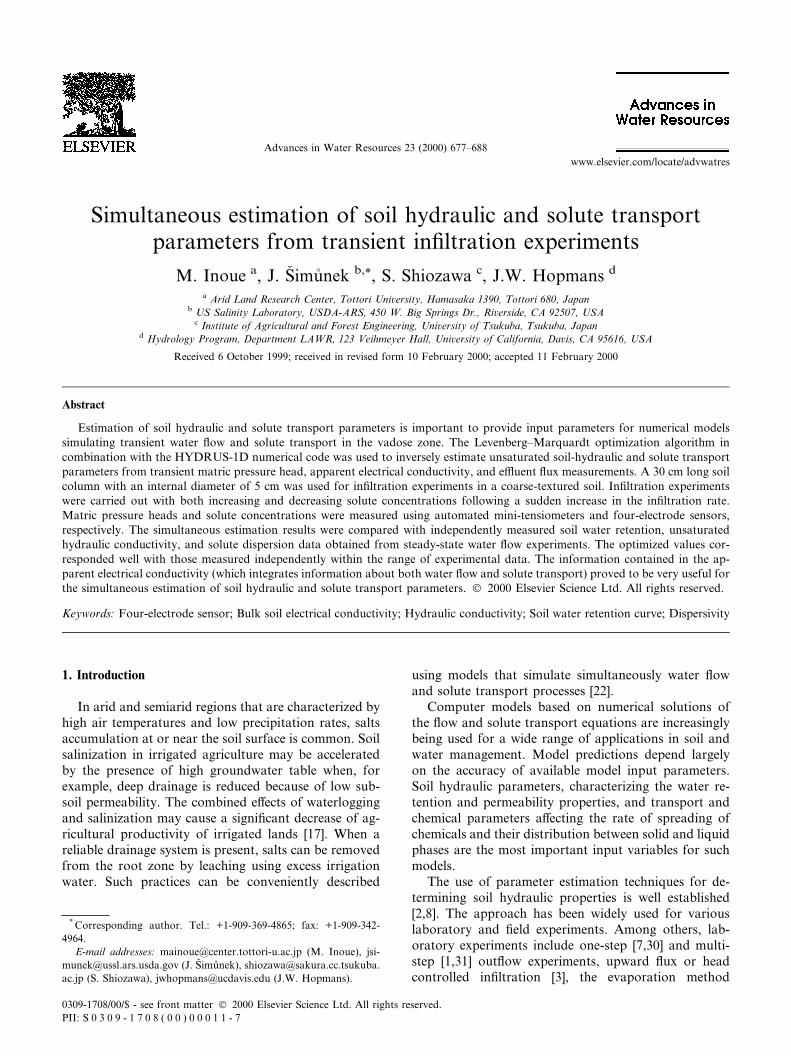
The four-electrode sensors were calibrated in mix-tures of Tottori dune sand and sodium chloride solu-
tions [4,21]. The measured bulk soil electricalconductivity (ECa) depends on the electrical conductiv-ity of the soil solution (ECw), the volumetric watercontent (h), the dry bulk density (qb), and temperatureof the water solution and the soil (T). After washing thesand with distilled water, clay and silt fractions wereremoved, and the pure sand samples were oven-dried.Clay and silt fractions were removed in order to preventpotential clogging and permeability changes of the po-rous plate by transport of these ®ner fractions during therelatively fast in®ltration experiments. Known volumesof NaCl solution with known concentrations were addedto the sand to obtain the desired water content and saltconcentration values. In all, four-electrode probe cali-bration was carried out for NaCl concentrations of0.005, 0.01, 0.02, 0.03, 0.04, 0.05, 0.06, 0.08, 0.1, 0.2, 0.5,and 1.0 mol/l, and for volumetric water content valuesranging from 0.0287 to 0.454 cm3/cm3, including fullsaturation. The mixtures were kept in a vinyl bag at aconstant temperature of 25°C for two days. A total of 96prepared soil samples were packed uniformly in columnsof 50 mm inside diameter and 60 mm height, and thesurfaces leveled and covered to prevent evaporation.After measurement of ECa with the four-electrode sen-sor, the volumetric water content and the dry bulkdensity of each soil sample were determined from oven-drying. The average value of the dry bulk density (qb)was 1.45 � 0.02 g/cm3 at an average soil temperature ofT� 25.0 � 0.5°C.
We assumed that the relation between ECa and ECw
can be described by the following relationship, whichneglects the surface conductance of the solid phase [17]
ECa
h� a�ECw � h� � b: �12�
The surface conductance, associated with the ex-changeable ions at the solid±liquid interface, can beneglected only for sandy soil. Rhoades and Oster [18]discussed relations between ECa and ECw for situationswhen the surface conductance cannot be neglected, suchas for silt and clay fractions. The ®tted relations of ECa
versus h are shown in Fig. 2 for various solution con-centrations; symbols in the ®gure are experimental val-ues and the lines represent the ®tted Eq. (12). Fittedvalues for a and b were 1.45 and 0.102, respectively, witha correlation coe�cient value of 0.998.
To convert ECw to concentration, the following ex-perimentally derived power relationship was used [4]
C � 0:008465 � EC1:073w : �13�
Using Eq. (12), the water content can be determined ifthe pore water salinity, ECw, is known, or alternativelyECw can be computed from the measured ECa and aknown h. Average relative errors were calculated usingthe expression 100
P�jYm ÿ Yej=Ye�=n, where n, Ye andYm represent the number of experimental data, and
V1
V2
Cylinder ring
Electric mini-tensiometer
∼
Rf
21X datalogger
Fig. 1. The four-electrode sensor and the electric circuit.
680 M. Inoue et al. / Advances in Water Resources 23 (2000) 677±688
estimated and experimental values, respectively. Weobtained average errors of 2.41% and 5.60% for thevolumetric water content and the soil water electricalconductivity, respectively. Hence, the four-electrodeprobe can be conveniently used to measure either watercontent h or concentration C.
3.2. Steady-state in®ltration experiments
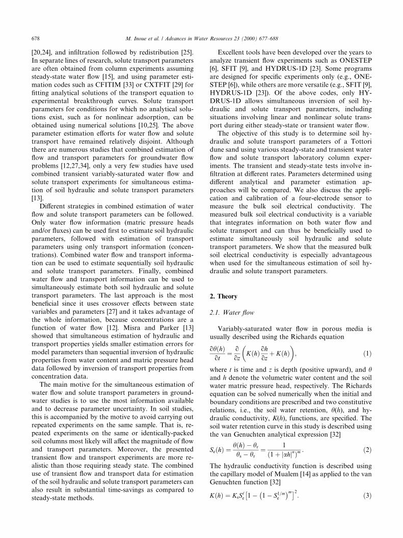
Four-electrode probes and mini-tensiometers wereused to determine the soil water retention curve fromsteady-state downward in®ltration into the washedTottori sand. The experimental setup consisted of a soilcolumn of 50 mm diameter and 30 cm height, and abalance to measure the drainage rate (Fig. 3) [34]. Thesoil column was packed under wet condition at the bulkdensity of 1:50� 0:03 g/cm3. Two mini-tensiometerswith pressure transducers and four-electrode sensorswere installed at the 13 and 23 cm depths, and an ad-ditional tensiometer at the 27 cm depth. A 5 mm thickcoarse-sintered glass plate with a saturated conductivityvalue of 0.000405 cm/s was placed at the bottom.
Using the syringe pump a constant in®ltration rate ofa NaCl solution having a constant concentration of 0.02mol/l was applied to the soil surface. After establishing asteady drainage rate at saturation, the in®ltration ratewas ®rst decreased in steps (to obtain drying retentiondata) and then increased (providing wetting retentiondata). Variations in the soil water matric pressure head(h) and the bulk electrical conductivity (ECa) with time
were measured using the mini-tensiometers and the four-electrode sensors, respectively. The matric pressure headat the bottom of the column was continuously adjustedto the value monitored by mini-tensiometer at the 23 cmdepth. Since the solution concentration (C) was knownand constant, ECw was determined directly from Eq.(13). Hence, the water content, h, could be estimateddirectly using Eq. (12) and the four-electrode sensor'smeasurement of ECa.
We then conducted a series of eight steady-state ¯owexperiments with steady-state in®ltration ¯uxes (i)varying between 0.022 and 0.00036 cm/s (®rst column ofTable 1). Using the steady-state data of the four-elec-trode sensors and mini-tensiometers at column depths of13 and 23 cm, unsaturated hydraulic conductivities, K,were calculated with Darcy's law from the knownsteady-state water ¯uxes and measured total hydraulichead gradients, dH/dz. Since ¯ow is steady state, thewater ¯ux is equal to the in®ltration rate at any columndepth. The results in Table 1 show that the hydraulicgradient dH/dz is near unity during each of the experi-ments, and that unsaturated hydraulic conductivity K isa rapidly decreasing function of h. The values of v, h, h,K, and dH/dz, presented in Table 1 are average valuesbetween depths of 13 and 23 cm.
Once steady-state water ¯ow was established over theentire soil column, the NaCl concentration of the in¯ow
Stop cock
23cm
13cm
Four-electrode sensor
Two-electrode sensor
Microtube pump
Electrical balance
Electric mini-tensiometer
Fig. 3. Schematic illustration of the column experimental setup.
Fig. 2. Calibration of the four-electrode sensor for dune sand. Lines
represent ®tted Eq. (2) for di�erent concentrations (di�erent electrical
conductivities of the soil solution as given in the legend), with the
highest concentration at the top and lowest at the bottom.
M. Inoue et al. / Advances in Water Resources 23 (2000) 677±688 681
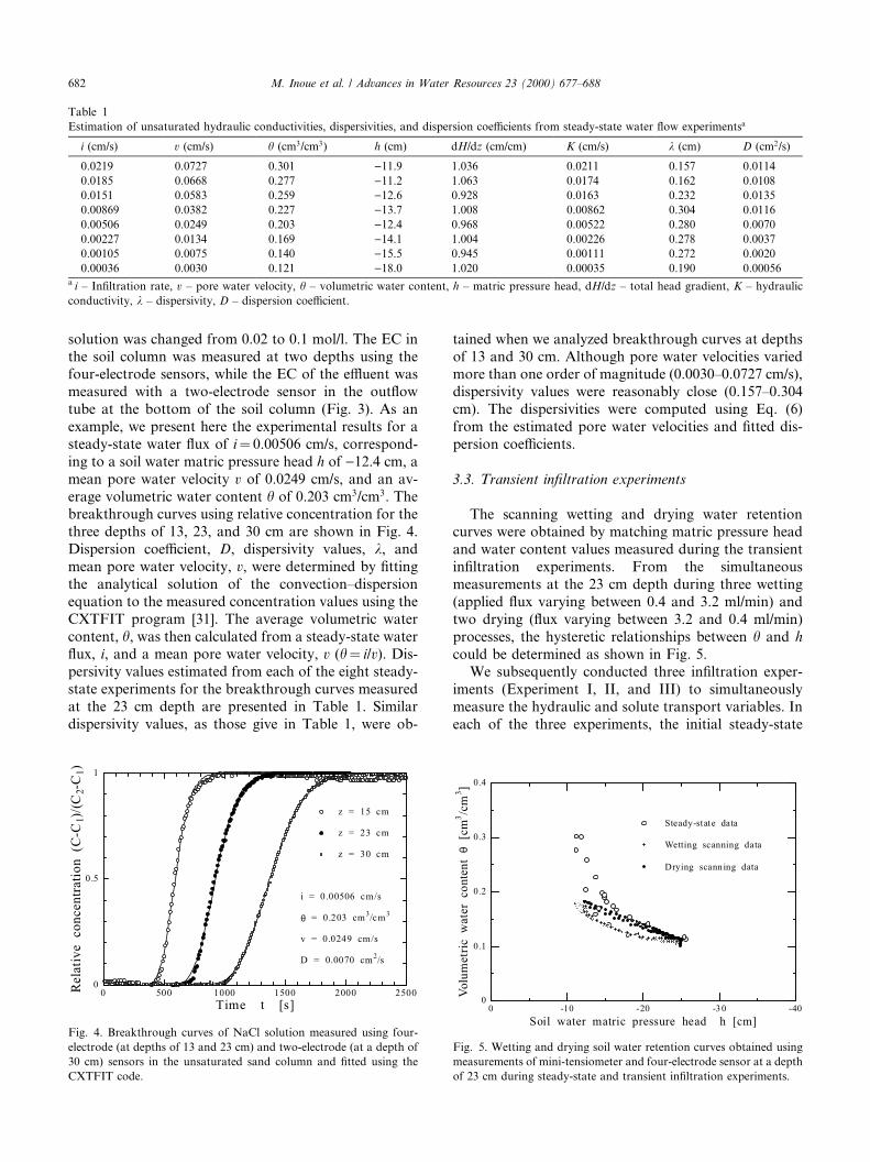
solution was changed from 0.02 to 0.1 mol/l. The EC inthe soil column was measured at two depths using thefour-electrode sensors, while the EC of the e�uent wasmeasured with a two-electrode sensor in the out¯owtube at the bottom of the soil column (Fig. 3). As anexample, we present here the experimental results for asteady-state water ¯ux of i� 0.00506 cm/s, correspond-ing to a soil water matric pressure head h of )12.4 cm, amean pore water velocity v of 0.0249 cm/s, and an av-erage volumetric water content h of 0.203 cm3/cm3. Thebreakthrough curves using relative concentration for thethree depths of 13, 23, and 30 cm are shown in Fig. 4.Dispersion coe�cient, D, dispersivity values, k, andmean pore water velocity, v, were determined by ®ttingthe analytical solution of the convection±dispersionequation to the measured concentration values using theCXTFIT program [31]. The average volumetric watercontent, h, was then calculated from a steady-state water¯ux, i, and a mean pore water velocity, v (h� i/v). Dis-persivity values estimated from each of the eight steady-state experiments for the breakthrough curves measuredat the 23 cm depth are presented in Table 1. Similardispersivity values, as those give in Table 1, were ob-
tained when we analyzed breakthrough curves at depthsof 13 and 30 cm. Although pore water velocities variedmore than one order of magnitude (0.0030±0.0727 cm/s),dispersivity values were reasonably close (0.157±0.304cm). The dispersivities were computed using Eq. (6)from the estimated pore water velocities and ®tted dis-persion coe�cients.
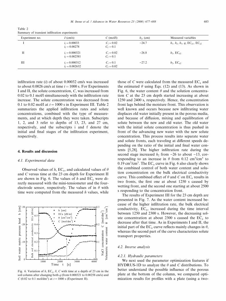
3.3. Transient in®ltration experiments
The scanning wetting and drying water retentioncurves were obtained by matching matric pressure headand water content values measured during the transientin®ltration experiments. From the simultaneousmeasurements at the 23 cm depth during three wetting(applied ¯ux varying between 0.4 and 3.2 ml/min) andtwo drying (¯ux varying between 3.2 and 0.4 ml/min)processes, the hysteretic relationships between h and hcould be determined as shown in Fig. 5.
We subsequently conducted three in®ltration exper-iments (Experiment I, II, and III) to simultaneouslymeasure the hydraulic and solute transport variables. Ineach of the three experiments, the initial steady-state
0 500 1000 1500 2000 2500
Time t [s]
0
0.5
1
Relative
concentration
(C-C
1)/(C
2-C
1)
z = 15 cm
z = 23 cm
z = 30 cm
i = 0.00506 cm/s
θ = 0.203 cm3/cm
3
v = 0.0249 cm/s
D = 0.0070 cm2/s
Fig. 4. Breakthrough curves of NaCl solution measured using four-
electrode (at depths of 13 and 23 cm) and two-electrode (at a depth of
30 cm) sensors in the unsaturated sand column and ®tted using the
CXTFIT code.
-40-30-20-100
Soil water matric pressure head h [cm]
0
0 .1
0 .2
0 .3
0 .4
Volumetric
watercontent
θ[cm
3/cm
3]
Drying scann ing data
Steady-state data
Wetting scanning data
Fig. 5. Wetting and drying soil water retention curves obtained using
measurements of mini-tensiometer and four-electrode sensor at a depth
of 23 cm during steady-state and transient in®ltration experiments.
Table 1
Estimation of unsaturated hydraulic conductivities, dispersivities, and dispersion coe�cients from steady-state water ¯ow experimentsa
i (cm/s) v (cm/s) h (cm3/cm3) h (cm) dH/dz (cm/cm) K (cm/s) k (cm) D (cm2/s)
0.0219 0.0727 0.301 )11.9 1.036 0.0211 0.157 0.0114
0.0185 0.0668 0.277 )11.2 1.063 0.0174 0.162 0.0108
0.0151 0.0583 0.259 )12.6 0.928 0.0163 0.232 0.0135
0.00869 0.0382 0.227 )13.7 1.008 0.00862 0.304 0.0116
0.00506 0.0249 0.203 )12.4 0.968 0.00522 0.280 0.0070
0.00227 0.0134 0.169 )14.1 1.004 0.00226 0.278 0.0037
0.00105 0.0075 0.140 )15.5 0.945 0.00111 0.272 0.0020
0.00036 0.0030 0.121 )18.0 1.020 0.00035 0.190 0.00056a i ± In®ltration rate, v ± pore water velocity, h ± volumetric water content, h ± matric pressure head, dH/dz ± total head gradient, K ± hydraulic
conductivity, k ± dispersivity, D ± dispersion coe�cient.
682 M. Inoue et al. / Advances in Water Resources 23 (2000) 677±688
in®ltration rate (i) of about 0.00032 cm/s was increasedto about 0.0026 cm/s at time t� 1000 s. For ExperimentsI and II, the solute concentration, C, was increased from0.02 to 0.1 mol/l simultaneously with the in®ltration rateincrease. The solute concentration was decreased from0.1 to 0.02 mol/l at t� 1000 s in Experiment III. Table 2summarizes the applied in®ltration rates and soluteconcentrations, combined with the type of measure-ments, and at which depth they were taken. Subscripts1, 2, and 3 refer to depths of 13, 23, and 27 cm,respectively, and the subscripts i and f denote theinitial and ®nal stages of the in®ltration experiment,respectively.
4. Results and discussion
4.1. Experimental data
Observed values of h, ECa, and calculated values of hand C versus time at the 23 cm depth for Experiment IIare shown in Fig. 6. The values of h and ECa were di-rectly measured with the mini-tensiometer and the four-electrode sensor, respectively. The values of in h withtime were computed from the measured h values, while
those of C were calculated from the measured ECa andthe estimated h using Eqs. (12) and (13). As shown inFig. 6, the water content h and the solution concentra-tion C at the 23 cm depth started increasing at about1250 and 2400 s, respectively. Hence, the concentrationfront lags behind the moisture front. This observation iswell known and occurs because new in®ltrating waterdisplaces old water initially present in the porous media,and because of di�usion, mixing and equilibration ofsolute between the new and old water. The old waterwith the initial solute concentration is thus pushed infront of the advancing new water with the new soluteconcentration. This process results into separate waterand solute fronts, each traveling at di�erent speeds de-pending on the ratio of the initial and ®nal water con-tents [5,28]. The higher in®ltration rate during thesecond stage increased h2 from )26 to about )13, cor-responding to an increase in h from 0.12 cm3/cm3 to0.19 cm3/cm3. The ECa curve in Fig. 6 also clearly showsthe combined control of both water content and solu-tion concentration on the bulk electrical conductivitycurve. This combined e�ect of h and C on ECa results intwo fronts, the ®rst one at about 1250 s caused bywetting front, and the second one starting at about 2500s responding to the concentration front.
The results of Experiment III for the 23 cm depth arepresented in Fig. 7. As the water content increased be-cause of the higher in®ltration rate, the bulk electricalconductivity, ECa, increased during the time intervalbetween 1250 and 2300 s. However, the decreasing sol-ute concentration at about 2300 s caused the ECa todecrease after that time. As in Experiments I and II, theinitial part of the ECa curve re¯ects mainly changes in h,whereas the second part of the curve characterizes solutetransport properties.
4.2. Inverse analysis
4.2.1. Hydraulic parametersWe next used the parameter optimization features if
HYDRUS-1D to analyze the h and C distributions. Tobetter understand the possible in¯uence of the porousplate at the bottom of the column, we compared opti-mization results for pro®les with a plate (using a two-
Table 2
Summary of transient in®ltration experiments
Experiment no. I (cm/s) C (mol/l) h2 i (cm) Measured variables
I ii� 0.00033 Ci� 0.02 )24.7 h1, h2, h3, q, ECa1, ECa2
if � 0.00278 Cf � 0.1
II ii� 0.000321 Ci� 0.02 )26.8 h2, ECa2
if � 0.002581 Cf � 0.1
III ii� 0.000312 Ci� 0.1 )27.2 h2, ECa2
if � 0.002632 Cf � 0.02
1000 2000 3000 4000
Time t [s]
-30
-20
-10
0Soil
watermatricpressure
head
h[cm]
0
0.1
0.2
0.3
Volumetric
watercontent
θ[cm
3/cm
3]
0.1
0.2
0.3
0.4
0.5
Bulk
soil
electricalco
nductivity
ECa
[dS/m
]
NaC
lco
ncen
tration
C[m
ol/dm
3]h [cm]
C [mol/dm3]
ECa [dS/m]
θ [cm3/cm
3]
Fig. 6. Variation of h, ECa, h, C with time at a depth of 23 cm in the
soil column after changing both q (from 0.000321 to 0.00258 cm/s) and
C (0.02 to 0.1 mol/dm3) at t� 1000 s (Experiment II).
M. Inoue et al. / Advances in Water Resources 23 (2000) 677±688 683
layer model) and without a plate (using a one-layermodel). The columns for this purpose were ®rst sche-matized as a two-layered pro®le with the Tottori sandrepresenting the ®rst layer and the sintered glass platerepresenting the second layer. The saturated hydraulicconductivity of the plate was independently measuredand found equal to 0.000405 cm/s. Fig. 8 shows the
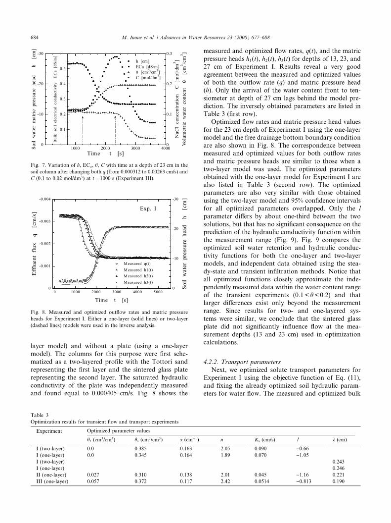
measured and optimized ¯ow rates, q(t), and the matricpressure heads h1(t), h2(t), h3(t) for depths of 13, 23, and27 cm of Experiment I. Results reveal a very goodagreement between the measured and optimized valuesof both the out¯ow rate (q) and matric pressure head(h). Only the arrival of the water content front to ten-siometer at depth of 27 cm lags behind the model pre-diction. The inversely obtained parameters are listed inTable 3 (®rst row).
Optimized ¯ow rates and matric pressure head valuesfor the 23 cm depth of Experiment I using the one-layermodel and the free drainage bottom boundary conditionare also shown in Fig. 8. The correspondence betweenmeasured and optimized values for both out¯ow ratesand matric pressure heads are similar to those when atwo-layer model was used. The optimized parametersobtained with the one-layer model for Experiment I arealso listed in Table 3 (second row). The optimizedparameters are also very similar with those obtainedusing the two-layer model and 95% con®dence intervalsfor all optimized parameters overlapped. Only the lparameter di�ers by about one-third between the twosolutions, but that has no signi®cant consequence on theprediction of the hydraulic conductivity function withinthe measurement range (Fig. 9). Fig. 9 compares theoptimized soil water retention and hydraulic conduc-tivity functions for both the one-layer and two-layermodels, and independent data obtained using the stea-dy-state and transient in®ltration methods. Notice thatall optimized functions closely approximate the inde-pendently measured data within the water content rangeof the transient experiments (0.1 < h < 0.2) and thatlarger di�erences exist only beyond the measurementrange. Since results for two- and one-layered sys-tems were similar, we conclude that the sintered glassplate did not signi®cantly in¯uence ¯ow at the mea-surement depths (13 and 23 cm) used in optimizationcalculations.
4.2.2. Transport parametersNext, we optimized solute transport parameters for
Experiment I using the objective function of Eq. (11),and ®xing the already optimized soil hydraulic param-eters for water ¯ow. The measured and optimized bulk
0 1000 2000 3000 4000 5000
Time t [s]
-0.004
-0.003
-0.002
-0.001
0
Effluentflux
q[cm/s]
-30
-20
-10
0 Soil
waterpressure
head
h[cm]
Measured q(t)
Measured h1(t)
Measured h2(t)
Measured h3(t)
Exp. I
Fig. 8. Measured and optimized out¯ow rates and matric pressure
heads for Experiment I. Either a one-layer (solid lines) or two-layer
(dashed lines) models were used in the inverse analysis.
Table 3
Optimization results for transient ¯ow and transport experiments
Experiment Optimized parameter values
hr (cm3/cm3) hs (cm3/cm3) a (cmÿ1) n Ks (cm/s) l k (cm)
I (two-layer) 0.0 0.385 0.163 2.05 0.090 )0.66
I (one-layer) 0.0 0.345 0.164 1.89 0.070 )1.05
I (two-layer) 0.243
I (one-layer) 0.246
II (one-layer) 0.027 0.310 0.138 2.01 0.045 )1.16 0.221
III (one-layer) 0.057 0.372 0.117 2.42 0.0514 )0.813 0.190
1000 2000 3000 4000
Time t [s]
-30
-20
-10
0
Soil
watermatric
pressure
head
h[cm]
0
0.1
0.2
0.3
Volumetric
watercontent
θ[cm
3/cm
3]
0.1
0.2
0.3
0.4
0.5
Bulk
soil
electricalconductivity
ECa
[dS/m
]
NaClconcentration
C[m
ol/dm
3]h [cm]
ECa [dS/m]
θ [cm3/cm
3]
C [mol/dm3]
Fig. 7. Variation of h, ECa, h, C with time at a depth of 23 cm in the
soil column after changing both q (from 0.000312 to 0.00263 cm/s) and
C (0.1 to 0.02 mol/dm3) at t� 1000 s (Experiment III).
684 M. Inoue et al. / Advances in Water Resources 23 (2000) 677±688

soil electrical conductivities, ECa1(t) and ECa2(t), atdepths of 13 and 23 cm, respectively, are presented inFig. 10. As discussed above, the initial small increase ofthe bulk soil electrical conductivity corresponds with thearrival of the moisture front, whereas the second, steeperand larger increase corresponds with the concentrationfront. Excellent agreement was obtained between themeasured and optimized ECa-values. The optimizeddispersivities k were equal to 0.246 and 0.243 cm using aone- and two-layer models, respectively. This shows thatthe porous plate also did not signi®cantly a�ect thedispersivity. Fig. 11 compares the optimized dispersioncoe�cients with the independently measured valuesobtained with the steady-state column experiments(Table 1). Again, notice the excellent agreement between
dispersion coe�cients obtained from transient andsteady-state experiments.
4.2.3. Simultaneous optimization of hydraulic and trans-port parameters
The next case involves transient Experiment II, againwith an increasing in®ltration ¯ux and increasing soluteconcentration, for which hydraulic and solute transportparameters were optimized simultaneously using theone-layer model. The optimized and measured matricpressure heads and bulk soil electrical conductivities forthe 23 cm depth are presented in Fig. 12. As indicatedearlier, this ®gure also clearly shows that the positions ofthe wetting and solute fronts are distinct, with theirpositions being a function of the initial water content.
10-3 5 10
-2 5 10-1
Mean pore water velocity v [cm/s]
10-4
10-3
10-2
10-1
Dispersion
coefficient
D[cm
2/s]
measured D(v)
λ=0.243 (Exp.I two layer model)
λ=0.246 (Exp.I one layer model)
λ=0.221 (Exp.II one layer model)
λ=0.190 (Exp III one layer model)
Fig. 11. The dispersion coe�cient D as function of the mean pore
water velocity v obtained by inverse optimization and from analysis of
steady-state data.
1000 2000 3000 4000
Time t [s]
-40
-30
-20
-10
0Soil
watermatric
pressure
head
h[cm]
0
0.2
0.4
0.6
0.8
Bulk
soil
electricalco
nductivity
ECa
[dS/m
]
Measured h(t)
Optimized h(t)
Measured ECa(t)
Optimized ECa(t)
Exp. II
Fig. 12. Measured and optimized matric pressure heads and bulk
electrical conductivities for Experiment II. A one-layer model was used
in the inverse analysis.
0 1000 2000 3000 4000 5000
Time t [s]
0
0.1
0.2
0.3
0.4
0.5
0.6
Bulk
soil
electricalconductivity
ECa
[dS/m
]
Measured ECa1(t)
Measured ECa2(t)
Optim ized ECa1(t)
Optim ized ECa2(t)
Exp. I
Fig. 10. Measured and optimized bulk electrical conductivities for
Experiment I. A one-layer model was used in the inverse analysis.
0 0.1 0.2 0.3 0.4 0.5
Volumetric water content θ [cm3/cm
3]
-40
-30
-20
-10
0Soil
watermatric
pressure
head
h[cm]
10-5
10-4
10-3
10-2
10-1
Hydraulic
conductivity
K[cm/s]
h(θ) Steady-state data
K(θ) Steady-state data
h(θ ) Transient (wet scan)
Measurement range
Fig. 9. Comparison between soil hydraulic properties estimated in-
versely for Experiment I using either a one- (solid lines) or two-layer
(dashed lines) models and those obtained from analysis of steady-state
and transient in®ltration data.
M. Inoue et al. / Advances in Water Resources 23 (2000) 677±688 685

Since the initial (hi) and ®nal (hf ) water contents wereabout 0.12 and 0.19, and the initial (ii) and ®nal (if )in®ltration rates about 0.00032 and 0.00258, re-spectively, one may expect the wetting front (fw) to moveabout 2.7 times faster than the concentration front (fs):
fw � if ÿ ii
if
:hf
hf ÿ hi
� �fs: �14�
This means that the center of the concentration frontshould arrive approximately 2.7 times later than thewetting front at some location in the column. Themeasured centers of the wetting and concentrationfronts (de®ned here as the arithmetic averages of theinitial and ®nal values of the matric pressure head andthe concentration, respectively) reached the 23 cm depthat 640 and 1780 s after the change in the in®ltration rate,respectively. Thus, the concentration front arrived about2.78 times later than the wetting front, which agrees wellwith the estimated value of 2.7, according to Eq. (14).Therefore, information contained in the two fronts doesnot overlap and can be used to advantage for thesimultaneous estimation of soil hydraulic and solutetransport parameters. Fig. 13 compares the inverselyestimated hydraulic functions against the independentlymeasured data. Notice again the excellent correspon-dence of the optimized retention curve and the transientwetting data within the experimental range. Optimiza-tion results are also presented in Table 3.
Finally, we optimized simultaneously the hydraulicand solute transport parameters to data from Experi-ment III, i.e., the experiment in which the in®ltrationrate was increased (from 0.000312 to 0.00263 cm/s) andthe solute concentration decreased (from 0.1 to 0.02mol/l) at t� 1000 s. The comparison of measured andsimulated h and EC data at the 23 cm column depth is
shown in Fig. 14. Again, excellent agreement exists be-tween the optimized and measured soil water matricpressure heads, h(t), and bulk soil electrical conductivi-ties, ECa(t). Similarly as for Experiment II, the waterfront moved about 2.7 times faster than the concentra-tion front. The optimized soil hydraulic functions arecompared in Fig. 13 with optimization results based onExperiment II, and with the independently measuredretention and hydraulic conductivity data. While there isa very good correspondence between the hydraulicconductivities obtained from the di�erent experiments,the optimized retention curve for Experiment III isslightly shifted towards higher water contents as com-pared with the curve for Experiment II. The parameterestimates are again presented in Table 3. The optimizeddispersivity value, however, compares again very wellwith the independently measured values and with theoptimized values from the other in®ltration experiments(Fig. 11).
5. Summary and conclusions
Matric pressure head and solute concentration weresimultaneously measured during in®ltration of sodiumchloride solution using mini-tensiometers with pressuretransducers and four-electrode sensors. Both the tensi-ometers and four-electrode sensors proved to be usefulfor measuring the rapid changes in matric pressure headand electrical conductivity during the simultaneousmovement of water and solute in the sandy soil columns.The bulk soil electrical conductivity (ECa) depends onthe solution electrical conductivity (ECw) and the volu-metric water content (h). After calibrating the functionalrelation of ECa� f(ECw, h) for each soil, ECw can beobtained from the measured ECa and the known h.
0 0.1 0.2 0.3 0.4 0.5
Volumetric water content θ [cm3/cm
3]
-40
-30
-20
-10
0Soil
watermatric
pressure
head
h[cm]
10-5
10-4
10-3
10-2
10-1
Hydraulic
conductivity
K[cm/s]
h(θ ) Transient (wet scan)
h(θ ) Steady-state data
K(θ) Steady-state data
Measurement range
Fig. 13. Comparison between soil hydraulic properties estimated in-
versely for Experiments II (solid lines) and III (dashed lines) using a
one-layer model and obtained from analysis of steady-state and tran-
sient in®ltration data (data points).
1000 2000 3000 4000
Time t [s]
-40
-30
-20
-10
0Soil
watermatric
pressure
head
h[cm]
0
0.2
0.4
0.6
0.8
Bulk
soil
electrical
conductivity
ECa
[dS/m
]
Measured h(t)
Optimized h(t)
Measured ECa(t)
Optimized ECa(t)
Exp. III
Fig. 14. Measured and optimized matric pressure heads and bulk
electrical conductivities for Experiment III. A one-layer model was
used in the inverse analysis.
686 M. Inoue et al. / Advances in Water Resources 23 (2000) 677±688

Alternatively, h can be obtained from the measured ECa
and a known ECw. In either case, ECa can be measuredaccurately using the calibrated four-electrode sensor.The more complex functional relation would be neededfor ®ner textured soils [18].
The Levenberg±Marquardt algorithm [11] in combi-nation with the HYDRUS-1D (version 2.0) [23] codewas used to inversely estimate the unsaturated soil hy-draulic and solute transport parameters from transientmatric pressure head, soil bulk electrical conductivityand ¯ux measurements. Experiments were carried outwith both increasing and decreasing solute concentra-tions following a sudden increase in the in®ltration ratein a sand-®lled column. Optimization results werecompared with independently measured soil water re-tention, unsaturated hydraulic conductivity and solutedispersion data. The optimized values corresponded wellwith those measured independently within the exper-imental range. Larger di�erences between ®ttedfunctions existed only outside the measurement range.However, it is generally accepted that parameters ob-tained with parameter estimation are to be used onlywithin the measurement range for which they weredetermined [24].
Since the apparent electrical conductivity, ECa, inte-grates information about both water ¯ow and solutetransport, information imbedded in ECa proved to bevery useful for the simultaneous estimation of the soilhydraulic and solute transport parameters. In®ltrationexperiments produced two distinctive fronts for watermovement and solute transport, and thus the e�ects ofwater content and concentration changes could be welldistinguished. Application of the parameter estimationtechnique, which combines a numerical solution of thegoverning partial di�erential equations with the Leven-berg±Marquardt method, to transient water ¯ow andsolute transport data resulted in accurate estimation ofthe soil hydraulic and solute transport parameters. Thecombined use of transient ¯ow and transport data forestimation of the soil hydraulic and solute transportparameters resulted in substantial timesaving as com-pared to steady-state methods. The presented methodwith simultaneous measurement of water ¯ow and sol-ute transport variables using a four-electrode probe andcoupled estimation of soil hydraulic and solute transportparameters can be a very e�cient method for multi-di-mensional ®eld experiments as well.
References
[1] Eching SO, Hopmans JW, Wendroth O. Unsaturated hydraulic
conductivity from transient multi-step out¯ow and soil water
pressure data. Soil Sci Soc Am J 1994;58:687±95.
[2] Hopmans JW, �Simunek J. Review of inverse estimation of soil
hydraulic properties. In: van Genuchten MTh, Leij FJ, Wu L,
editors. Characterization and measurement of the hydraulic
properties of unsaturated porous media. University of California,
Riverside, CA, 1999, p. 643±59.
[3] Hudson DB, Wierenga PJ, Hills RG. Unsaturated hydraulic
properties from upward ¯ow into soil cores. Soil Sci Soc Am J
1996;60:388±96.
[4] Inoue M. Simultaneous movement of salt and water in an
unsaturated sand column. ALRCÕs Annual Report 1993±94, Arid
Land Research Center, Tottori University, 1994. p. 1±26.
[5] Kirda C, Nielsen DR, Biggar JW. Simultaneous transport of
chloride and water during in®ltration. Soil Sci Soc Am Proc
1973;37(3):339±45.
[6] Kool JB, Parker JC, van Genuchten MTh. ONESTEP: A
nonlinear parameter estimation program for evaluating soil
hydraulic properties from one-step out¯ow experiments. Virginia
Agric Exp Stat Bull 1985;85(3).
[7] Kool JB, Parker JC, van Genuchten MTh. Determining soil
hydraulic properties from one-step out¯ow experiments by
parameter estimation: I. Theory and numerical studies. Soil Sci
Soc Am J 1985b;49:1348±54.
[8] Kool JB, Parker JC, van Genuchten MTh. Parameter estimation
for unsaturated ¯ow and transport models ± a review. J Hydrol
1987;91:255±93.
[9] Kool JB, Parker JC. Estimating soil hydraulic properties from
transient ¯ow experiments: SFIT user's guide. Electric Power
Research Institute Report, Palo Alto, CA, 1987.
[10] Kool JB, Parker JC, Zelazny LW. On the estimation of cation
exchange parameters from column displacement experiments. Soil
Sci Soc Am J 1989;53:1347±55.
[11] Marquardt DW. An algorithm for least-squares estimation of
nonlinear parameters. SIAM J Appl Math 1963;11:431±41.
[12] Medina A, Carrera J. Coupled estimation of ¯ow and solute
transport parameters. Water Resour Res 1996;32(10):3063±76.
[13] Mishra S, Parker JC. Parameter estimation for coupled
unsaturated ¯ow and transport. Water Resour Res
1989;25(3):385±96.
[14] Mualem Y. A new model for predicting the hydraulic conductiv-
ity of unsaturated porous media. Water Resour Res 1976;12:513±
22.
[15] Nkedi-Kizza P, Biggar JW, Selim HM, van Genuchten MTh,
Wierenga PJ, Davidson JM, Nielsen DR. On the equivalence of
two conceptual models for describing ion exchange during
transport through an aggregated oxisol. Water Resour Res
1984;20:1123±30.
[16] Rhoades JD. Instrumental ®eld methods of salinity appraisal. In:
Topp GC, Reynolds WD, Green RE, editors. Advances in
measurement of soil physical properties: bringing theory into
practice. SSSA Special Pub. No. 30, 1992. p. 231±48.
[17] Rhoades JD. Sustainability of irrigation: an overview of salinity
problems and control strategies. CWRA 1997 Annual Conference
Footprints of Humanity: Re¯ections on 50 Years of Water
Resource Developments, Lethbridge, Alberta, Canada, 3±6 June
1997. p. 1±42.
[18] Rhoades JD, Oster JD. Solute content, In: Klute A, editor.
Method of soil analysis part 1. 2nd ed. SSSA, Madison, WI, 1986.
p. 985±94.
[19] Robbins CW. Field and laboratory measurements. In: Tanji KK,
editor. Agricultural salinity assessment and management. ASCE
Manuals and Reports on Engineering Practice No. 71, 1990.
p. 201±04.
[20] Santini A, Romano N, Ciollaro G, Comegna V. Evaluation of a
laboratory inverse method for determining unsaturated hydraulic
properties of a soil under di�erent tillage practices. Soil Sci
1995;160:340±51.
[21] Shiozawa S, Inoue M, Toride N. Solute transport under unsat-
urated unit gradient water ¯ow monitored in soil columns. Soil Sci
Soc Am J, submitted.
M. Inoue et al. / Advances in Water Resources 23 (2000) 677±688 687
[22] �Sim�unek J, Suarez DL. Sodic soil reclamation using multicom-
ponent transport modeling. ASCE J Irrig Drain Eng
1997;123(5):367±76.
[23] �Sim�unek J, �Sejna M, van Genuchten MTh. The HYDRUS-1D
software package for simulating water ¯ow and solute transport in
two-dimensional variably saturated media. Version 2.0, IGWMC
± TPS ± 70, International Ground Water Modeling Center,
Colorado School of Mines, Golden, CO, 1998.
[24] �Sim�unek J, Wendroth O, van Genuchten MT. A parameter
estimation analysis of the evaporation method for determin-
ing soil hydraulic properties. Soil Sci Soc Am J 1998b;62(4):894±
905.
[25] �Sim�unek J, van Genuchten MTh. Using the HYDRUS-1D and
HYDRUS-2D codes for estimating unsaturated soil hydraulic and
solute transport parameters. In: vanGenuchten MTh, Leij FJ, Wu
L, editors. Characterization and measurement of the hydraulic
properties of unsaturated porous media. University of California,
Riverside, CA, 1999. p. 1523±36.
[26] �Sim�unek J, Hopmans JW. Parameter optimization and nonlinear
®tting. In: Dane JH, Topp GC, editors. Methods of soil analysis,
part 1. physical methods. 3rd ed. SSSA, Madison, WI, 2000.
[27] Sun N-Z, Yeh WW-G. Coupled inverse problems in groundwater
modeling. 1. Sensitivity analysis and parameter identii®cation.
Water Resour Res 1990;26(10):2507±25.
[28] Smiles DE, Philip JR, Knight JH, Elrick DE. Hydrodynamic
dispersion during absorption of water by soil. Soil Sci Soc Am J
1978;42:229±34.
[29] Toride N, Leij FJ, vanGenuchten MTh. The CXTFIT code for
estimating transport parameters from laboratory or ®eld tracer
experiments. Version 2.0, Research Report No. 137, US Salinity
Laboratory, USDA, ARS, Riverside, CA, 1995.
[30] van Dam JC, Stricker JNM, Droogers P. Inverse method for
determining soil hydraulic functions from one-step out¯ow
experiment. Soil Sci Soc Am J 1992;56:1042±50.
[31] van Dam JC, Stricker JNM, Droogers P. Inverse method to
determine soil hydraulic functions from multistep out¯ow exper-
iment. Soil Sci Soc Am J 1994;58:647±52.
[32] van Genuchten MTh. A closed-form equation for predicting the
hydraulic conductivity of unsaturated soils. Soil Sci Soc Am J
1980;44:892±8.
[33] van Genuchten MTh. Non-equilibrium transport parameters from
miscible displacement experiments. Research Report No. 119, US
Salinity Laboratory, USDA, ARS, Riverside, CA, 1981.
[34] Weiss R, Smith L. Parameter space methods in joint parameter
estimation for groundwater ¯ow models. Water Resour Res
1998;34(4):647±61.
688 M. Inoue et al. / Advances in Water Resources 23 (2000) 677±688