Simultaneous Chandra X ray, Hubble Space Telescope ... · PDF fileSimultaneous Chandra X ray, Hubble Space Telescope ultraviolet, and Ulysses radio observations of Jupiter’s aurora

Simultaneous Chandra X ray, Hubble Space Telescope ultraviolet,

and Ulysses radio observations of Jupiter’s aurora

R. F. Elsner,1 N. Lugaz,2 J. H. Waite Jr.,2 T. E. Cravens,3 G. R. Gladstone,4 P. Ford,5

D. Grodent,6 A. Bhardwaj,1,7 R. J. MacDowall,8 M. D. Desch,8 and T. Majeed2

Received 3 August 2004; revised 30 September 2004; accepted 5 November 2004; published 14 January 2005.

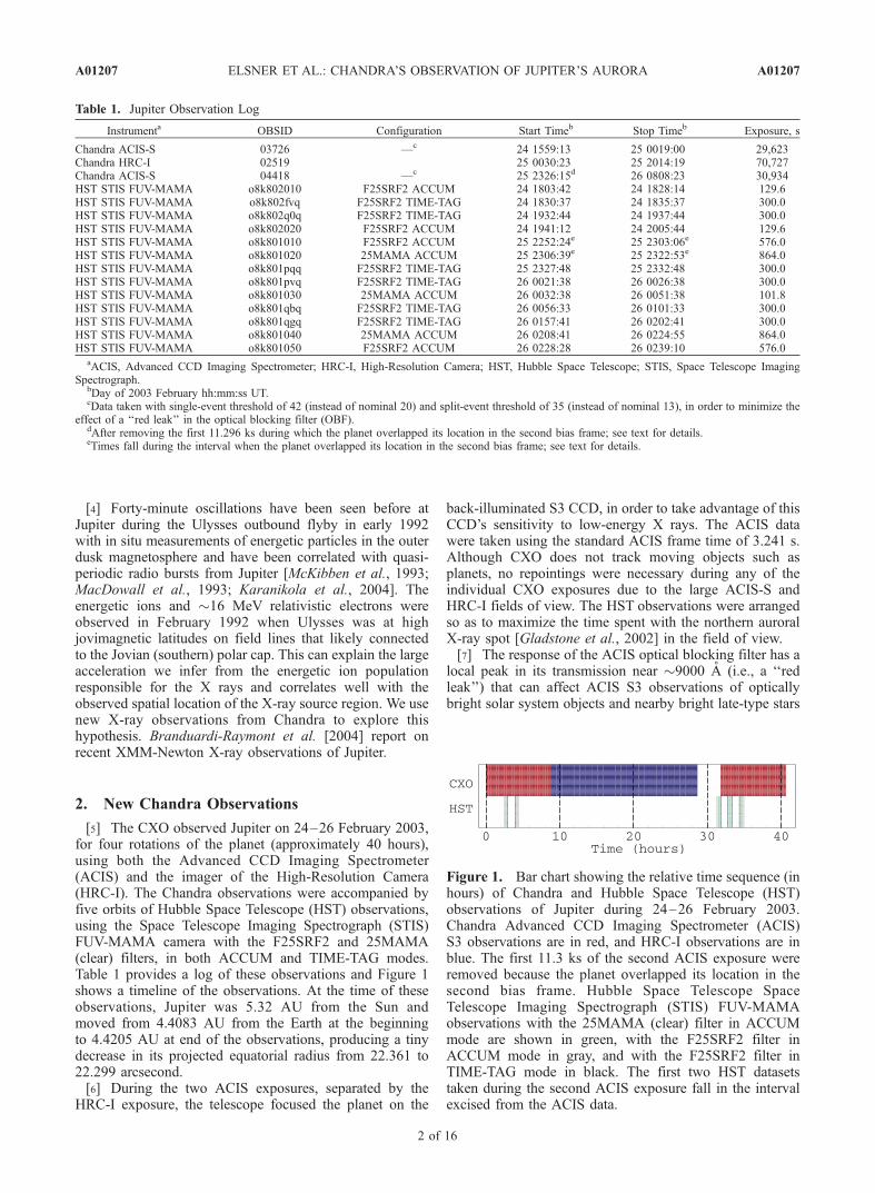
[1] Observations of Jupiter carried out by the Chandra Advanced CCD ImagingSpectrometer (ACIS-S) instrument over 24–26 February 2003 show that the auroral X-rayspectrum consists of line emission consistent with high-charge states of precipitatingions, and not a continuum as might be expected from bremsstrahlung. The part of thespectrum due to oxygen peaks around 650 eV, which indicates a high fraction of fullystripped oxygen in the precipitating ion flux. A combination of the OVIII emission lines at653 eV and 774 eV, as well as the OVII emission lines at 561 eV and 666 eV, are evidentin the measure auroral spectrum. There is also line emission at lower energies in thespectral region extending from 250 to 350 eV, which could be from sulfur and/or carbon.The Jovian auroral X-ray spectra are significantly different from the X-ray spectra ofcomets. The charge state distribution of the oxygen ions implied by the measured auroralX-ray spectra strongly suggests that independent of the source of the energetic ions,magnetospheric or solar wind, the ions have undergone additional acceleration. Thisspectral evidence for ion acceleration is also consistent with the relatively high intensitiesof the X rays compared with the available phase space density of the (unaccelerated)source populations of solar wind or magnetospheric ions at Jupiter, which are orders ofmagnitude too small to explain the observed emissions. The Chandra X-ray observationswere executed simultaneously with observations at ultraviolet wavelengths by the HubbleSpace Telescope and at radio wavelengths by the Ulysses spacecraft. These additionaldata sets suggest that the source of the X rays is magnetospheric in origin and that theprecipitating particles are accelerated by strong field-aligned electric fields, whichsimultaneously create both the several-MeV energetic ion population and the relativisticelectrons observed in situ by Ulysses that are correlated with �40 min quasi-periodic radiooutbursts.

Citation: Elsner, R. F., et al. (2005), Simultaneous Chandra X ray, Hubble Space Telescope ultraviolet, and Ulysses radio

observations of Jupiter’s aurora, J. Geophys. Res., 11 0 , A01207, doi:10.1029/2004JA010717.

1. Introduction

[2] Jupiter is a powerful source of X rays within our solarsystem [Bhardwaj et al., 2002]. Early observations revealedboth a high-latitude source of X rays associated withJupiter’s aurora [Metzger et al., 1983; Waite et al., 1994]and a low-latitude source associated with particle precipi-

tation from the radiation belts and/or scattered solar X rays[Waite et al., 1997; Maurellis et al., 2000]. More recentobservations on 18 December 2000 [Gladstone et al.,2002], using the Chandra X Ray Observatory’s (CXO)High-Resolution Camera (HRC-I) instrument and the Hub-ble Space Telescope’s Space Telescope Imaging Spectro-graph (STIS) instrument, pinpointed most of the auroralX rays to a small high-latitude region that mapped alongmagnetic field lines into the outer Jovian magnetodisk at>30 Jovian radii from Jupiter. The northern auroral X-rayemissions observed with the HRC in December 2000 weretightly confined in longitude between 160 and 180 degreesSIII and in latitude between 60 and 70 degrees and thus werestrongly correlated with the Jovian magnetic field.[3] A surprising feature of the auroral X-ray light

curve from the 18 December 2000 CXO observations [seeGladstone et al., 2000, Figure 2, upper panel] was asignificant 40-min oscillation in the north (and perhaps alsoin the south). However, the HRC counting statistics in thesouth did not permit determination of the relative phase ofthe oscillations in the north and south.

JOURNAL OF GEOPHYSICAL RESEARCH, VOL. 110, A01207, doi:10.1029/2004JA010717, 2005

1NASA Marshall Space Flight Center, Huntsville, Alabama, USA.2Department of Atmospheric, Oceanic, and Space Sciences, University

of Michigan, Ann Arbor, Michigan, USA.3Department of Physics and Astronomy, University of Kansas,

Lawrence, Kansas, USA.4Southwest Research Institute, San Antonio, Texas, USA.5Center for Space Research, Massachusetts Institute of Technology,

Cambridge, Massachusetts, USA.6Institut d’Astrophysique et de Geophysique, Universite de Liege,

Liege, Belgium.7On leave from Space Physics Laboratory, Vikram Sarabhai Space

Centre, Trivandrum, India.8NASA Goddard Space Flight Center, Greenbelt, Maryland, USA.

Copyright 2005 by the American Geophysical Union.0148-0227/05/2004JA010717$09.00

A01207 1 of 16

[4] Forty-minute oscillations have been seen before atJupiter during the Ulysses outbound flyby in early 1992with in situ measurements of energetic particles in the outerdusk magnetosphere and have been correlated with quasi-periodic radio bursts from Jupiter [McKibben et al., 1993;MacDowall et al., 1993; Karanikola et al., 2004]. Theenergetic ions and �16 MeV relativistic electrons wereobserved in February 1992 when Ulysses was at highjovimagnetic latitudes on field lines that likely connectedto the Jovian (southern) polar cap. This can explain the largeacceleration we infer from the energetic ion populationresponsible for the X rays and correlates well with theobserved spatial location of the X-ray source region. We usenew X-ray observations from Chandra to explore thishypothesis. Branduardi-Raymont et al. [2004] report onrecent XMM-Newton X-ray observations of Jupiter.

2. New Chandra Observations

[5] The CXO observed Jupiter on 24–26 February 2003,for four rotations of the planet (approximately 40 hours),using both the Advanced CCD Imaging Spectrometer(ACIS) and the imager of the High-Resolution Camera(HRC-I). The Chandra observations were accompanied byfive orbits of Hubble Space Telescope (HST) observations,using the Space Telescope Imaging Spectrograph (STIS)FUV-MAMA camera with the F25SRF2 and 25MAMA(clear) filters, in both ACCUM and TIME-TAG modes.Table 1 provides a log of these observations and Figure 1shows a timeline of the observations. At the time of theseobservations, Jupiter was 5.32 AU from the Sun andmoved from 4.4083 AU from the Earth at the beginningto 4.4205 AU at end of the observations, producing a tinydecrease in its projected equatorial radius from 22.361 to22.299 arcsecond.[6] During the two ACIS exposures, separated by the

HRC-I exposure, the telescope focused the planet on the

back-illuminated S3 CCD, in order to take advantage of thisCCD’s sensitivity to low-energy X rays. The ACIS datawere taken using the standard ACIS frame time of 3.241 s.Although CXO does not track moving objects such asplanets, no repointings were necessary during any of theindividual CXO exposures due to the large ACIS-S andHRC-I fields of view. The HST observations were arrangedso as to maximize the time spent with the northern auroralX-ray spot [Gladstone et al., 2002] in the field of view.[7] The response of the ACIS optical blocking filter has a

local peak in its transmission near �9000 A (i.e., a ‘‘redleak’’) that can affect ACIS S3 observations of opticallybright solar system objects and nearby bright late-type stars

Table 1. Jupiter Observation Log

Instrumenta OBSID Configuration Start Timeb Stop Timeb Exposure, s

Chandra ACIS-S 03726 —c 24 1559:13 25 0019:00 29,623Chandra HRC-I 02519 25 0030:23 25 2014:19 70,727Chandra ACIS-S 04418 —c 25 2326:15d 26 0808:23 30,934HST STIS FUV-MAMA o8k802010 F25SRF2 ACCUM 24 1803:42 24 1828:14 129.6HST STIS FUV-MAMA o8k802fvq F25SRF2 TIME-TAG 24 1830:37 24 1835:37 300.0HST STIS FUV-MAMA o8k802q0q F25SRF2 TIME-TAG 24 1932:44 24 1937:44 300.0HST STIS FUV-MAMA o8k802020 F25SRF2 ACCUM 24 1941:12 24 2005:44 129.6HST STIS FUV-MAMA o8k801010 F25SRF2 ACCUM 25 2252:24e 25 2303:06e 576.0HST STIS FUV-MAMA o8k801020 25MAMA ACCUM 25 2306:39e 25 2322:53e 864.0HST STIS FUV-MAMA o8k801pqq F25SRF2 TIME-TAG 25 2327:48 25 2332:48 300.0HST STIS FUV-MAMA o8k801pvq F25SRF2 TIME-TAG 26 0021:38 26 0026:38 300.0HST STIS FUV-MAMA o8k801030 25MAMA ACCUM 26 0032:38 26 0051:38 101.8HST STIS FUV-MAMA o8k801qbq F25SRF2 TIME-TAG 26 0056:33 26 0101:33 300.0HST STIS FUV-MAMA o8k801qgq F25SRF2 TIME-TAG 26 0157:41 26 0202:41 300.0HST STIS FUV-MAMA o8k801040 25MAMA ACCUM 26 0208:41 26 0224:55 864.0HST STIS FUV-MAMA o8k801050 F25SRF2 ACCUM 26 0228:28 26 0239:10 576.0

aACIS, Advanced CCD Imaging Spectrometer; HRC-I, High-Resolution Camera; HST, Hubble Space Telescope; STIS, Space Telescope ImagingSpectrograph.

bDay of 2003 February hh:mm:ss UT.cData taken with single-event threshold of 42 (instead of nominal 20) and split-event threshold of 35 (instead of nominal 13), in order to minimize the

effect of a ‘‘red leak’’ in the optical blocking filter (OBF).dAfter removing the first 11.296 ks during which the planet overlapped its location in the second bias frame; see text for details.eTimes fall during the interval when the planet overlapped its location in the second bias frame; see text for details.

Figure 1. Bar chart showing the relative time sequence (inhours) of Chandra and Hubble Space Telescope (HST)observations of Jupiter during 24–26 February 2003.Chandra Advanced CCD Imaging Spectrometer (ACIS)S3 observations are in red, and HRC-I observations are inblue. The first 11.3 ks of the second ACIS exposure wereremoved because the planet overlapped its location in thesecond bias frame. Hubble Space Telescope SpaceTelescope Imaging Spectrograph (STIS) FUV-MAMAobservations with the 25MAMA (clear) filter in ACCUMmode are shown in green, with the F25SRF2 filter inACCUM mode in gray, and with the F25SRF2 filter inTIME-TAG mode in black. The first two HST datasetstaken during the second ACIS exposure fall in the intervalexcised from the ACIS data.

A01207 ELSNER ET AL.: CHANDRA’S OBSERVATION OF JUPITER’S AURORA

2 of 16

A01207

[ Elsner et al., 2002]. Thre e steps were taken to reduce thisproblem to a manageable level for our Jupiter observations.[8] First, the bias frame (normally used to determine the

background and subtract it on board CXO) was taken withthe planet off the S3 CCD during the first ACIS-S obser-vation. This avoided the appearance of a brightness‘‘bump’’ in the bias frame due to optical light from thebright planetary disk. Since the image of Jupiter movedacross the detector during the �8 hour ACIS observation, anormal bias image would have been worse than useless.Unfortunately, the planet remained in the field of view whiletaking the bias frame for the second ACIS observation,requiring us to excise the first 11.3 ks of data, during whichthe planet overlapped the bump in the bias frame. Two ofthe HST entries in Table 1 fell during this excised interval,as noted in footnote 4 to the table.[9] Second, the single- and split-event thresholds for the

ACIS S3 CCD were raised to 42 and 35, respectively(instead of the nominal values of 20 and 13), in order toavoid saturating the count rate with artificial X-ray eventsinduced by the planet’s bright optical emission.[10] Third, the data were taken in Timed Exposure, Very

Faint mode which records pulse-height-amplitudes in five-by-five pixel islands and permits a careful correction of thepulse-height-amplitude data for any residual optical effectsusing a specialized procedure developed by one of us(PGF). In this procedure, a local mean bias value iscomputed by averaging the 16 smallest pulse-height ampli-tudes from the 25 pixels of the event island. The appropriatebias frame values are added back into the amplitudes in theinner nine pixels and the local mean bias value subtracted.The data are then reprocessed using the standard CIAO toolacis.process.events in order to calculate corrected eventgrades, pulse-invariant channel values, and event energies.In our analysis, after applying this correction, we keep onlythe standard ASCA grades 0, 2, 3, 4, and 6. Owing to thisnecessary procedure, the single-pixel (grade 0) spectrumstarts at �100 eV, the two-pixel spectrum at �168 eV, thethree-pixel spectrum at �236 eV, and the four-pixel spec-trum at �300 eV. There are very few five-pixel events. Sofor the spectral analysis we employ a low-energy cutoff at300 eV (which made the distinction between carbon andsulfur lines in the observed spectra much harder) and use thestandard response matrix for our spectral analyses, keepingin mind there may still be a tendency to undercount thehigher grades (more pixel) events at the low end of ourband. Charge-transfer-inefficiency (CTI) effects are minimalfor the back-illuminated S3 CCD, and no CTI correctionswere made.[11] The ACIS S3 and HRC-I data were transformed into

a frame of reference centered on Jupiter using appropriateephemerides data obtained from the JPL HORIZONS pro-gram and Chandra orbit ancillary data provided in the dataproducts from the Chandra X-ray Center (CXC).[12] The ACIS-S 300–2000 eV count rate within a 1.05

Jupiter equatorial radius, averaged over both exposures, is0.034 counts per second. The equivalent background countrate for events outside a 1.2 Jupiter equatorial radius, RJ,rescaled to a circle with radius 1.05 RJ, is 0.00088 countsper second, showing the effectiveness of Very Faint modefor suppressing background. In addition, the planet blocksX rays emitted from distant sources. Therefore for the ACIS

data and the corresponding spectral analysis, we do notsubtract background. The HRC-I count rate within a 1.05 RJ

is 0.044 counts per second, while the equivalent backgroundrate derived from a region outside 1.2 RJ is 0.014 countsper second. Cosmic rays and radioactive decay within theHRC-I’s microchannel plate are the principal sources ofHRC-I background and thus are not blocked by the planet.The equivalent rates for the 18 December 2000 HRC-Idata were 0.080 counts per second within 1.05 RJ and0.012 counts per second background. Thus the planet wassignificantly dimmer in X rays during the 24–26 February2003 observations compared to the 18 December 2000observations.[13] For spectral modeling it is necessary to take account

of the time-dependent contamination layer on the ACISoptical blocking filter [Plucinsky et al., 2003]. We do this bymultiplying the ACIS S3 effective area by an energy-dependent correction factor calculated using the CIAO toolacisabs. The resulting effective area curve is shown in thetop panel of Figure 3 (see section 3). We also carry outthe spectral analysis correcting for contamination by usingthe energy-dependent effective area correction factor calcu-lated using the contamarf tool (H. L. Marshall, privatecommunications, 2003). The spectral modeling results areindistinguishable using these two different contaminationcorrection methods.

3. Spectral Analysis of the ACIS Data Set

[14] To analyze the spectral data the disk was divided, asshown in Figure 2, into three areas of interest: (1) the northernauroral zone, (2) the southern auroral zone, and (3) the disk(excluding the auroral zones). Following the preprocessingnecessary for the spectral data described in section 2, spectralfiles, suitable for fitting in XSPEC [Arnaud, 1996] using theresponse and effective area files described above, weregenerated using LEXTRCT (A. F. Tennant, private commu-nication, 2004). The measured X-ray spectra, which includethe instrumental response, for the north and south auroralzones are shown in the middle two panels of Figure 3, wherethey can be compared with the ACIS-S effective area curve(top panel) and cometary X-ray spectra (bottom panel). Thelower-latitude disk spectra will be described in a separatepaper. The ACIS background rate derived from the 300–2000 eVevents located outside 1.2 Jupiter radii and scaled tothe area of the planetary disk is <3% of the emission from thetotal disk. In addition, the background contribution for trueX rays from beyond Jupiter’s orbit is blocked by the planet.As a result, we neglect the background in our spectralanalysis of the ACIS data.[15] We judge the acceptability of our spectral fits using

the c2 statistic for an appropriate number of degrees offreedom v (equal to the number of data points minus thenumber of fit parameters). Throughout this section wealso provide the probability that statistical chance wouldyield an equivalent data set for which the same ‘‘fittingmodel’’ gives a c2 value greater than (i.e., a worse fit) thecalculated/actual value. For example, for a value of c2 witha probability of 5%, we can reject the model-data fit thatgave this value of c2 as unacceptable with, in this example,95% confidence. On the other hand, the fit is statisticallyacceptable if this probability is sufficiently large. Reduced


3 of 16

A01207

c2 is defined as the actual value of c2 divided by thenumber of degrees of freedom, v. Reduced c2 has anexpected mean value of unity, independent of the value of v.[16] The measured Jovian auroral X-ray spectra (middle

two panels of Figure 3) have significant intensity levels intwo energy bands: (1) 500–800 eV, presumably fromoxygen transitions, and (2) 300–360 eV, probably fromsulfur transition (although carbon transitions cannot beexcluded, as will be discussed later in this section). Thecount rate in the 380–500 eV part of the auroral spectrum isrelatively low. Emission also appears to exist below 300 eV,but we exclude this lower energy emission in our discussiondue to concerns about the effect of our event regrading onthe ACIS spectral response discussed earlier, see section 2.A comparison of the observed auroral spectra with theACIS-S effective area curve (top panel of Figure 3) reveals

some simple but important facts. The ACIS-S effective areacurve exhibits a sharp drop at �290 eV due to the presenceof carbon in the optical blocking filter and absorption justabove carbon K-edge at 284 eV. Above this edge theeffective area rises relatively smoothly toward the oxygenK-edge at 532 eV. The relatively strong emission below350 eV together with the corresponding deficit of X rays inthe auroral spectrum over the 380–500 eV band aretherefore inconsistent with a continuum spectrum, suchas would be produced by a bremsstrahlung mechanism.We explicitly demonstrated this by fitting the thermalbremsstrahlung model available in XSPEC to the northauroral spectrum. The fitting parameters are the plasmatemperature and a normalization; the model assumes cosmicabundances. Although the best-fit temperature value,�250 eV, is in agreement with results from ROSAT PSPC

Figure 2. Color-coded image of ACIS-S (0.25–2.0 keV) events from 24–26 February 2003observations as seen in a frame moving across the sky with Jupiter, smoothed with a two-dimensionalgaussian with s = 0.738 arcsec (1.5 ACIS pixel width). The white scale bar in the lower right represents5 arcsec, and the small circles near the center represent the sub-Earth and subsolar points. Thesuperimposed graticule shows latitude and longitude lines at intervals of 30�. For spectral analysis, northand south auroral events are defined as inside the white circle with radius 1.05 the Jovian equatorialradius and outside the white box, while disk events are defined as inside both the circle and the box.The total 0.25–2.0 keV count rate inside the dashed circle is 0.034 counts per second, while that within0.75 Jovian radii but scaled to the size of the planet is 0.024 counts per second. The equivalentbackground rate derived from events more than 1.2 Jovian radii from the planet’s center and scaled to thesize of the planet is 0.00088 counts per second, showing the effectiveness of Very Faint mode forsuppressing background. The color bar for the figure is in Rayleighs (R).


4 of 16

A01207

data [Waite et al., 1994], the fit is extremely poor with avalue for c2 of 91.1, a reduced c2 of 5.36, and a probabilityfor chance occurrence greater than this value of 3.9 �10�12. This fit is shown with the data in the second panelof Figure 3. Comparison of the fit with the data suggests tous that no reasonable continuum model alone can hope toreproduce the shape of the measured spectrum. An electronbremsstrahlung mechanism is also very unlikely on ener-

getic grounds [cf. Bhardwaj and Gladstone, 2000, andreferences therein].[17] Line emission seems the more likely explanation for

most of the observed auroral X-ray emission. Table 2provides a list of possible lines from carbon, sulfur, andoxygen that are present in the 300–800 eV soft X-ray partof the spectrum. Oxygen lines from OVII (that is, O6+)and OVIII (i.e., O7+) are plausible candidates for the 500–

Figure 3. (a) ACIS-S effective area versus energy in kev, including the effects of contamination onthe optical blocking filter at the time of the observations. (b) and (c) Jovian auroral X-ray spectrabetween 300 eV and 1 keV of the north auroral region (Figure 3b) and the south auroral region(Figure 3c) as defined in Figure 2, for the first ACIS-S observation. The vertical dotted line at0.3 keV shows the low-energy cutoff for the Jovian spectra. Each spectral point represents�10 measured events. The solid line in Figure 3b shows the best-fit thermal bremsstrahlung model tothe measured northern auroral spectrum. This result demonstrates that bremsstrahlung in particular,and probably any reasonable continuum model alone, cannot account for the observed spectrum. Thelower global count as well as number of events of the south auroral zone compared to the north areclearly visible. (d) Chandra ACIS-S spectrums of comets Linear S4 [S4] and McNaught-Hartley[MH]; note that the spectrum for comet MH is plotted after scaling by a factor of 0.5. Twonoticeable features present in Jovian spectra but absent (or very much weaker) in the cometaryspectra are located at around 0.65 keV and 0.75 keV.


5 of 16

A01207

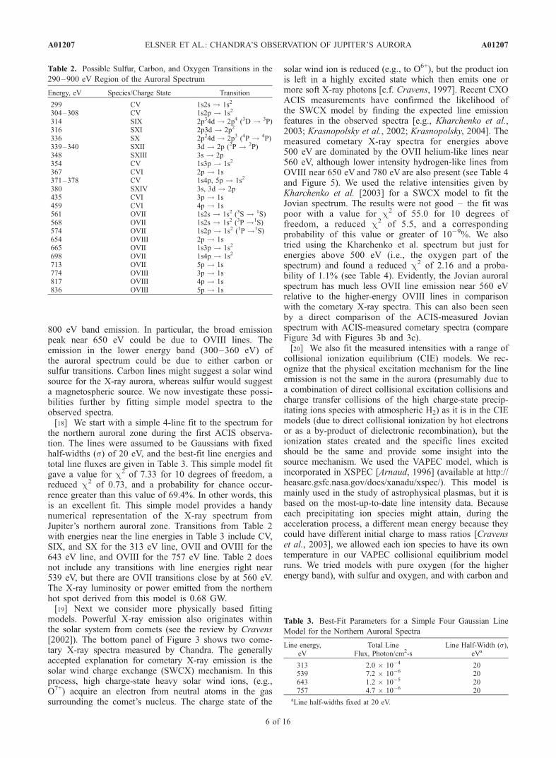
800 eV band emission. In particular, the broad emissionpeak near 650 eV could be due to OVIII lines. Theemission in the lower energy band (300–360 eV) ofthe auroral spectrum could be due to either carbon orsulfur transitions. Carbon lines might suggest a solar windsource for the X-ray aurora, whereas sulfur would suggesta magnetospheric source. We now investigate these possi-bilities further by fitting simple model spectra to theobserved spectra.[18] We start with a simple 4-line fit to the spectrum for

the northern auroral zone during the first ACIS observa-tion. The lines were assumed to be Gaussians with fixedhalf-widths (s) of 20 eV, and the best-fit line energies andtotal line fluxes are given in Table 3. This simple model fitgave a value for c2 of 7.33 for 10 degrees of freedom, areduced c2 of 0.73, and a probability for chance occur-rence greater than this value of 69.4%. In other words, thisis an excellent fit. This simple model provides a handynumerical representation of the X-ray spectrum fromJupiter’s northern auroral zone. Transitions from Table 2with energies near the line energies in Table 3 include CV,SIX, and SX for the 313 eV line, OVII and OVIII for the643 eV line, and OVIII for the 757 eV line. Table 2 doesnot include any transitions with line energies right near539 eV, but there are OVII transitions close by at 560 eV.The X-ray luminosity or power emitted from the northernhot spot derived from this model is 0.68 GW.[19] Next we consider more physically based fitting

models. Powerful X-ray emission also originates withinthe solar system from comets (see the review by Cravens[2002]). The bottom panel of Figure 3 shows two come-tary X-ray spectra measured by Chandra. The generallyaccepted explanation for cometary X-ray emission is thesolar wind charge exchange (SWCX) mechanism. In thisprocess, high charge-state heavy solar wind ions, (e.g.,O7+) acquire an electron from neutral atoms in the gassurrounding the comet’s nucleus. The charge state of the

solar wind ion is reduced (e.g., to O6+), but the product ionis left in a highly excited state which then emits one ormore soft X-ray photons [c.f. Cravens, 1997]. Recent CXOACIS measurements have confirmed the likelihood ofthe SWCX model by finding the expected line emissionfeatures in the observed spectra [e.g., Kharchenko et al.,2003; Krasnopolsky et al., 2002; Krasnopolsky, 2004]. Themeasured cometary X-ray spectra for energies above500 eV are dominated by the OVII helium-like lines near560 eV, although lower intensity hydrogen-like lines fromOVIII near 650 eV and 780 eV are also present (see Table 4and Figure 5). We used the relative intensities given byKharchenko et al. [2003] for a SWCX model to fit theJovian spectrum. The results were not good – the fit waspoor with a value for c2 of 55.0 for 10 degrees offreedom, a reduced c2 of 5.5, and a correspondingprobability of this value or greater of 10�9%. We alsotried using the Kharchenko et al. spectrum but just forenergies above 500 eV (i.e., the oxygen part of thespectrum) and found a reduced c2 of 2.16 and a proba-bility of 1.1% (see Table 4). Evidently, the Jovian auroralspectrum has much less OVII line emission near 560 eVrelative to the higher-energy OVIII lines in comparisonwith the cometary X-ray spectra. This can also been seenby a direct comparison of the ACIS-measured Jovianspectrum with ACIS-measured cometary spectra (compareFigure 3d with Figures 3b and 3c).[20] We also fit the measured intensities with a range of

collisional ionization equilibrium (CIE) models. We rec-ognize that the physical excitation mechanism for the lineemission is not the same in the aurora (presumably due toa combination of direct collisional excitation collisions andcharge transfer collisions of the high charge-state precip-itating ions species with atmospheric H2) as it is in the CIEmodels (due to direct collisional ionization by hot electronsor as a by-product of dielectronic recombination), but theionization states created and the specific lines excitedshould be the same and provide some insight into thesource mechanism. We used the VAPEC model, which isincorporated in XSPEC [Arnaud, 1996] (available at http://heasarc.gsfc.nasa.gov/docs/xanadu/xspec/). This model ismainly used in the study of astrophysical plasmas, but it isbased on the most-up-to-date line intensity data. Becauseeach precipitating ion species might attain, during theacceleration process, a different mean energy because theycould have different initial charge to mass ratios [Cravenset al., 2003], we allowed each ion species to have its owntemperature in our VAPEC collisional equilibrium modelruns. We tried models with pure oxygen (for the higherenergy band), with sulfur and oxygen, and with carbon and

Table 2. Possible Sulfur, Carbon, and Oxygen Transitions in the

290–900 eV Region of the Auroral Spectrum

Energy, eV Species/Charge State Transition

299 CV 1s2s ! 1s2

304–308 CV 1s2p ! 1s2

314 SIX 2p34d ! 2p4 (3D ! 3P)316 SXI 2p3d ! 2p2

336 SX 2p24d ! 2p3 (4P ! 4P)339–340 SXII 3d ! 2p (2P ! 2P)348 SXIII 3s ! 2p354 CV 1s3p ! 1s2

367 CVI 2p ! 1s371–378 CV 1s4p, 5p ! 1s2

380 SXIV 3s, 3d ! 2p435 CVI 3p ! 1s459 CVI 4p ! 1s561 OVII 1s2s ! 1s2 (3S ! 1S)568 OVII 1s2s ! 1s2 (3P !1S)574 OVII 1s2p ! 1s2 (1P !1S)654 OVIII 2p ! 1s665 OVII 1s3p ! 1s2

698 OVII 1s4p ! 1s2

713 OVII 5p ! 1s774 OVIII 3p ! 1s817 OVIII 4p ! 1s836 OVIII 5p ! 1s

Table 3. Best-Fit Parameters for a Simple Four Gaussian Line

Model for the Northern Auroral Spectra

Line energy,eV

Total LineFlux, Photon/cm2-s

Line Half-Width (s),eVa

313 2.0 � 10�4 20539 7.2 � 10�6 20643 1.2 � 10�5 20757 4.7 � 10�6 20

aLine half-widths fixed at 20 eV.


6 of 16

A01207

oxygen. The fit parameters are therefore the differentplasma temperatures for the different species, the carbonor sulfur over oxygen ratio, and a normalization factor. Weremind the reader that the temperature values derivedbelow are not physical. Rather they are a representativeparameterization for the ionization states probably respon-sible for the X-ray emission.[21] Figures 4 and 5 show the data fits for the sulfur-

oxygen and carbon-oxygen CIE models, respectively.Actually, two VAPEC models were run in each case (onefor each species) and the results combined to fit the data.Both these fits were much more successful than the com-etary model, mainly because the CIE models allowed a

higher abundance of OVIII than OVII (due to the freeoxygen temperature), whereas the OVIII to OVII ratio inthe cometary model was not a free parameter and thecometary ratio is evidently not appropriate for the Jovianaurora. For the sulfur-oxygen plasma case (Figure 6), thevalue for c2 was 11.51 for 15 degrees of freedom, thereduced c2 was 0.7673, with a chance probability of a thisvalue of c2 or greater being 71.6%. For the carbon-oxygenplasma case (Figure 7), the fit was significantly worse witha c2 of 23.6 for 15 degrees of freedom, a reduced c2 of1.575, and a probability of 7.2%. These fit results indicatethat a sulfur-oxygen ‘‘plasma’’ is more appropriate than acarbon-oxygen one as the source of the auroral X-ray

Table 4. Fit Parameters for the Spectral Region Between 500 and 900 eV for the Northern Auroral Spectra for

Various Models of the Line Emission Ratios

Energy, eV

Cometary ChargeTransfer Intensity-Kharchenko’s

Fitted Intensity–Collisional

Equilibrium Modelwith Free Charge-State

Abundance Transitions

560 ± 3 1 0.64 O6+ (n = 2 ! 1)OVII 2 1,3P ! 1 1SOVII 2 3S ! 1 1S

650 ± 6 0.35 1.08 O6+ (n = 3 ! 1),OVII 3 1,3P ! 1 1SOVII 4 1P ! 1 1SO7+ (2p ! 1s)

OVIII 2 2P ! 1 2S780 ± 23 0.051 0.10 O7+ (3p,4p ! 1s)

OVIII 3,4 2P ! 1 2S845 ± 19 0.059 0.026 O7+ (4,5,6p ! 1s)

OVIII 5,6 2P ! 1 2S

Figure 4. Fit with two added VAPEC models of the north auroral zone emission between 300 eV and1 keV, for the first ACIS-S observation. The fitting parameters are the plasma temperatures of oxygen andsulfur, the ratio of sulfur over oxygen and a normalization factor. The VAPEC model assumes species arein collisional equilibrium. c2 is 11.51, the reduced c2 is 0.767, and the probability of chance occurrenceof this value for c2 or greater is 71.6%. The S/O ratio is 16.6 times the solar value, the oxygentemperature is 355 eV, and the sulfur temperature is 172 eV.


7 of 16

A01207

Figure 5. Fit with two added VAPEC models of the north auroral zone emission between 300 eV and1 keV, for the first ACIS-S observation. The fitting parameters are the plasma temperatures of oxygen andcarbon, the ratio of carbon over oxygen and a normalization factor. The VAPEC model assumes speciesthat are in collisional equilibrium. The c2 is 23.6, the reduced c2 is 1.57, and the probability of this valueof c2 or greater is 7.2%. The C/O ratio is 5.34 times the solar value, the oxygen temperature is 355 eV,and the carbon temperature is 81 eV.

Figure 6. Exposure map for the 24–26 February 2003 data, summed over both ACIS-S exposures andthe HRC-I exposure, in System III coordinates. The color scale was chosen to enhance contrast. Theminimum and maximum exposure times are 55 ks and 78 ks, respectively, occurring at the very highestlatitudes at the south and north poles. The exposure time varies by <16% over most of the map. Theoval at top shows the region in the north, and the rectangle at the bottom shows the region in thesouth, used for timing analysis. The oval is defined as a circle (on the sphere) centered at 67�N latitudeand 170� System III longitude with radius 6.5�. The rectangle lies between �67�S and �83�S latitudeand 306�–360� and 0�–116� System III longitude. The color bar of the figure is in kiloseconds.


8 of 16

A01207

emission. In both cases, oxygen lines are used to fit thehigher-energy part of the spectrum and there is littledifference between the two cases. However, it appearsthat it is easier to fit the auroral intensity in the 300–400 eV part of the spectrum with sulfur lines than withcarbon lines. These results favor a magnetospheric originover a solar wind origin for the energetic particles pre-sumed to be responsible for the X-ray aurora.[22] The best-fit VAPEC model has an oxygen tempera-

ture of 355 eV and a sulfur temperature of 172 eV, roughlyhalf the oxygen temperature. These fit temperatures arisefrom the charge state abundances in the CIE models whichare needed to produce lines in the correct locations in theauroral spectrum, and these abundances depend on thetemperature. The oxygen-sulfur temperature ratio is perhapssuggestive that the oxygen is accelerated to a higher energythan the sulfur (maybe due to a higher initial, preacceler-ated, charge-to-mass ratio in the magnetosphere). However,because the CIE model does not have the correct physics forthe Jovian aurora, verification of this supposition must awaitmore appropriate physical models of the aurora.[23] We now departed from the VAPEC model by allow-

ing the charge state ratios to deviate from those in colli-sional equilibrium but constraining the relative linestrengths within charge states to be those in collisionalequilibrium. In these fits we kept the 3–5 strongest linesfor each charge state. For the data above 500 eV, weobtained a reasonably good fit (c2 = 13.1 for 9 degrees of

freedom, reduced c2 = 1.457, and a probability of 14.8%)with 48% OVIII and 52% OVII. An even better fit can beobtained by boosting the abundance of the high principalquantum number (i.e., n = 5–6) OVIII lines near an energyof 850 eV (see Tables 2 and 4) by a factor of 6 over theVAPEC model. In this case, we obtain a c2 of 10.1, areduced c2 of 1.26, and a probability of 25.1% with the fitabundances of 42% OVIII and 58% OVII. What can welearn from the auroral spectrum at higher energies? Follow-ing arguments on charge state abundance versus beamenergy using measured phase space densities for both solarwind and magnetospheric origins presented by Cravens etal. [2003], the presence of high principal quantum numberOVIII lines argues for the acceleration of oxygen ions toenergies above 1 MeV per nucleon. At these high energies,the incident oxygen ions are stripped of most of theirelectrons [Cravens et al., 1995]. We will return to this inthe discussion section.[24] Now we further discuss the X-ray intensity between

300 eV and 500 eV. The intensity in the 360–500 eV bandis low, whereas the measured 300–360 eV count rate isrelatively high, especially considering the sharp drop inACIS effective area just above 290 eV due to the carbonK-edge. Both carbon and sulfur ion species have transi-tions in the 300–360 eV band (see Table 2). Again,carbon would suggest a solar wind origin whereas sulfurwould be consistent with a magnetospheric origin. BothC5+ and C6+ are abundant in the solar wind and the

Figure 7. Rate map for the 24–26 February 2003 data, 250–2000 eV, summed over both ACIS-Sexposures and the HRC-I exposure, in System III coordinates, convolved with a two-dimensionalgaussian with s = 1.5�. The lines crossing the plot from 360� to 0� trace the feet of the Io flux tubeand the L = 30 flux tube, as defined by the VIP4 model, in the north and south hemispheres. The ovalat top shows the region in the north, and the rectangle at the bottom the region in the south, used fortiming analysis. The oval is defined as a circle (on the sphere) centered at 67�N latitude and 170�System III longitude with radius 6.5�. The rectangle lies between �67�S and �83�S latitude and306�–360� and 0�–116� System III longitude. The color bar of the figure is in counts per kilosecondper square degree.


9 of 16

A01207

observed cometary X-ray spectrum is known to have CVIand CV soft X-ray lines due to the SWCX mechanism [cf.Cravens, 2002; Kharchenko et al., 2003]. Carbon has alsobeen detected in the Jovian magnetosphere [e.g., Krimigisand Roelof, 1983; Lanzerotti et al., 1992], but its abun-dance is lower than that of oxygen and sulfur. Sulfur andoxygen are known to be very abundant in the Jovianmagnetosphere, although the initial magnetospheric chargestates are low (q = 1–3) in comparison with those neededto explain the X-ray observations. However, just as foroxygen, if magnetospheric carbon and sulfur ions areaccelerated to sufficient energies, then higher charge statesare produced by electron removal collisions upon impact-ing the Jovian atmosphere [cf. Cravens et al., 1995].Unfortunately, no detailed calculations have been under-taken for carbon and sulfur. Nonetheless, some inferencescan be drawn from Table 2 and model fitting exercises tothe observed spectrum.[25] A pure sulfur model fit to the spectrum between 300

and 500 eV, allowing the charge state abundances to befitting parameters but keeping the CIE relative line intensi-ties gives a fit with c2 = 2.0 for 2 degrees of freedom,reduced c2 = 1.0, and a probability of 37.0%. The lowcount rate in this band leads to large errors but the bestfit has a relative combined abundance of SX and SXI of90–95% and 5–10% SXIV (ignoring all energies above500 eV). A similar exercise for carbon gives a relativeabundance of CV of about 96% with only 4% CVI. Thislarge CV to CVI abundance ratio (required for a decentspectrum fit) presents a problem for either the solar wind

or the magnetospheric mechanisms because the solarwind is known to have a high C6+ abundance, leadingto CVI emission with the SWCX mechanism, andbecause for the magnetospheric case if most of theoxygen is O8+ or O7+, then most of the carbon shouldbe fully-stripped C6+.

4. Timing Analysis

[26] Strong quasi-periodic oscillations on a timescale of�45 min were clearly seen in the light curve and the powerspectral density (PSD) for the X-rays from Jupiter’s north-ern auroral zone observed with the HRC-I on 18 December2000 [Gladstone et al., 2002]. Quasi-periodic oscillationsat a similar timescale are sometimes seen in the Ulyssesradio data at 10s of kHz [MacDowall et al., 1993; R. J.MacDowall, private communication, 2003].[27] In order to search for such variations in the February

2003 Jupiter X-ray data, we first used the JPL Horizonsephemeris data to create an exposure map in System IIIcoordinates (Figure 6). Except at the most extreme latitudesnear the poles, the exposure time varies by <16% over mostof the map, this variation being due to the gap in coverageintroduced by removing the initial 11.3 ks from the secondACIS exposure.[28] We then extracted X-ray events from regions in the

northern and southern auroral zones. In System III coor-dinates (see Figure 7), the X-rays in the north are mostlyconfined to a hot spot, just as they were during the18 December 2000 observations. In order to study their

Figure 8. X ray count rate, in counts per kilosecond, for the northern (blue) and southern (red) auroralzones, created by 12-min boxcar smoothing of a 4-min binning of the data. The time origin correspondsto UT 1558:06 on 24 February 2003. The black vertical lines from top to bottom mark the transitionsfrom ACIS-S to HRC-I exposures and back to ACIS-S. A gap appears at the beginning of the secondACIS-S exposure because we excised data taken when Jupiter overlapped its location in the second biasframe. The bars at the top mark the simultaneous HST observations, color-coded as in Figure 1. Note thatthe set of exposures containing the UV flare coincides with the tallest peak in the ACIS-S light curve forthe northern auroral zone. Smooth sections of sine waves provide crude representations of projected areaeffects arising from the planet’s rotation.


10 of 16

A01207

variability, we extracted events from a circle (in sphericalcoordinates) on Jupiter’s surface centered at latitude 67�Nand 170� system III longitude with radius 6.5�. Chandra’sview of the southern polar regions was much better inFebruary 2003 than it was in December 2000. The X-rayauroral emissions in the south appear confined to a bandrather than a spot as in the north. For the south, we extractedevents in the band between �83� and �67�S latitude andbetween 306� to 360� and 0� to 116� in System IIIlongitude.[29] The HRC-I and ACIS-S count rates are comparable

(see section 2), so for the time-variability analysis weconstructed time series including both ACIS-S exposuresand the HRC-I exposure together. Since we are no longerconcerned with preserving the ACIS-S spectral response,the ACIS-S data were restricted to the slightly expandedenergy band 250–2000 eV. The HRC-I data include back-

ground, which is negligible for the ACIS-S data. Theresulting time series for the northern and southern auroralzones are shown in Figure 8. The X-ray emission from thetwo zones as observed by CXO are clearly not simulta-neous, with the peaks in the south displaced from those inthe north by roughly 1/3 the planet’s rotation period.However, in both zones the emission comes from thoseregions mapping to and beyond 30 RJ in the outer magne-tosphere. Since we cannot follow these regions as theyrotate around the planet, it remains possible that the appar-ent variations from each are correlated, which wouldindicate a common origin for both along the flux tubejoining them. There are also clear variations in the peakintensity from cycle to cycle. There are 417 X-ray events inthe light curve for the north and 397 X-ray events in thelight curve for the south.[30] In order to look for �45 min oscillations, and any

evidence for an additional link between the northern andsouthern auroral zones, we constructed three power spec-tral densities (PSD) for these data: (1) the northern lightcurve, (2) the southern light curve, and (3) the sum of thenorthern and southern light curves. These PSDs are shownin Figure 9 in the top, middle, and bottom panels,respectively. These PSDs were normalized, as suggestedby Leahy et al. [1983], so that for Poisson-distributed datawith sufficient counts, the dimensionless expectation valuefor the power at any frequency is two, and the distributionof power is c2 with two degrees of freedom. The dottedlines in the PSD plots show the single-frequency proba-bilities of chance occurrence, from bottom to top, of 0.1,0.01, 0.001, 0.0001, and 0.00001, calculated from thisdistribution.[31] All three PSDs show strong peaks related to

Jupiter’s rotation. None of them show evidence forquasi-periodic oscillations near 45 min, unlike the strong45-min quasi-periodicity seen in the HRC-I observationsin December 2000 [Gladstone et al., 2002]. However,there are suggestive peaks in all three PSDs within theperiod range 10–100 min (containing 217 independentfrequencies or periods). For each PSD, Table 5 lists theperiods in this interval with single-frequency probabilitiesof chance occurrence <0.001. The significance levelsquoted in the table take into account our search over217 independent periods. These results may be marginalevidence of a more chaotic time variability on timescalesmore or less close to 45 min.[32] In order to check whether the variation due to

Jupiter’s rotation and the gap in the second ACIS-Sexposure introduce artifacts into these PSDs, we con-structed a time series and PSD for all events outside thetwo auroral zones considered above (i.e., the disk X-rayemission). We found the PSD in the interval 10–100 mincompletely consistent with no significant time variability,as expected for emission most likely due to reflected andreprocessed solar X rays.

5. Comparison to Ulysses Radio Observations

[33] The Ulysses spacecraft is in a highly inclined,elliptical orbit with an aphelion of 5.4 AU, which some-times places it less than a few AU from Jupiter. At thesedistances, the Ulysses radio receivers frequently observe

Figure 9. Power spectral density (PSD) versus period(in min), computed from the unsmoothed 4-min binningof the data for the northern (top), southern (middle), andsum of the northern and southern (bottom) auroral zones,respectively. In each plot, the solid line shows theexpectation value for a steady source with Poisson statistics.The dotted lines show the single period probabilitiesof chance occurrence as labeled on the right. There are217 independent periods between 10 and 100 min (301 ineach complete PSD).


11 of 16

A01207

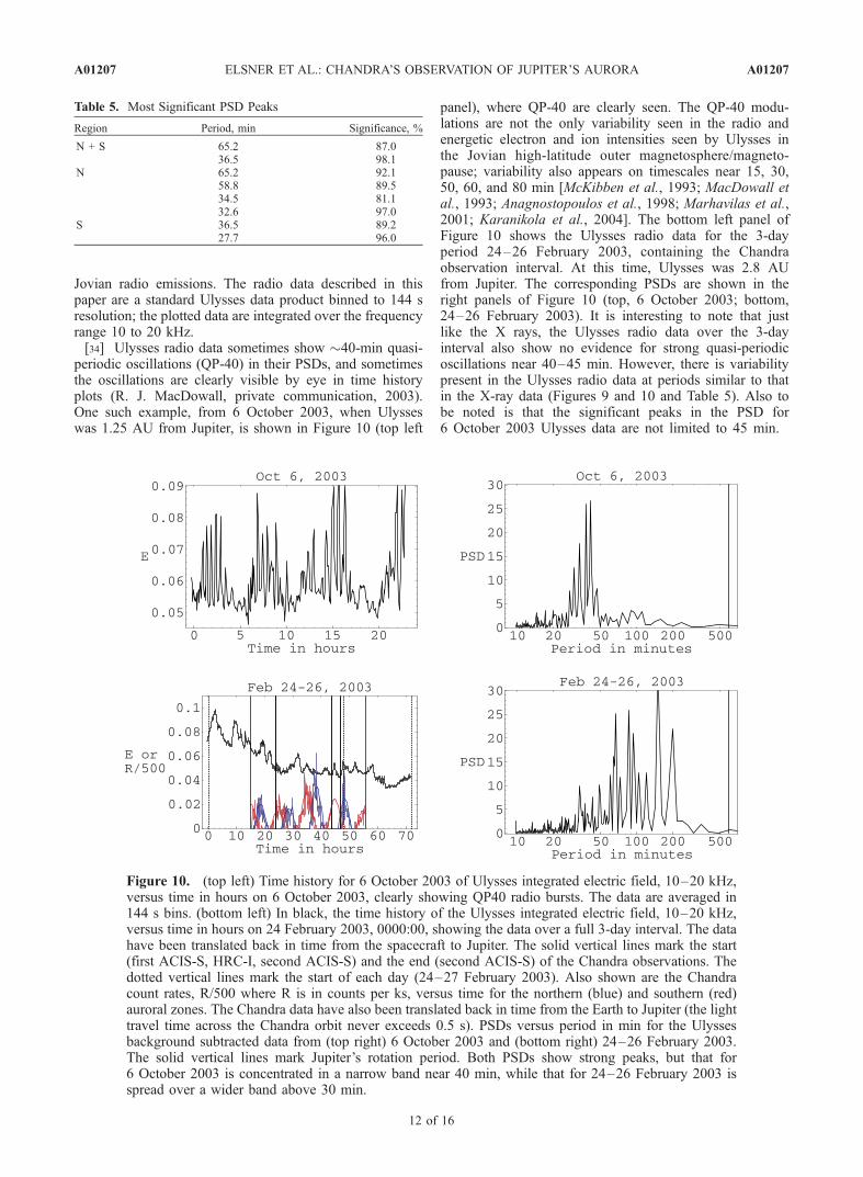
Jovian radio emissions. The radio data described in thispaper are a standard Ulysses data product binned to 144 sresolution; the plotted data are integrated over the frequencyrange 10 to 20 kHz.[34] Ulysses radio data sometimes show �40-min quasi-

periodic oscillations (QP-40) in their PSDs, and sometimesthe oscillations are clearly visible by eye in time historyplots (R. J. MacDowall, private communication, 2003).One such example, from 6 October 2003, when Ulysseswas 1.25 AU from Jupiter, is shown in Figure 10 (top left

panel), where QP-40 are clearly seen. The QP-40 modu-lations are not the only variability seen in the radio andenergetic electron and ion intensities seen by Ulysses inthe Jovian high-latitude outer magnetosphere/magneto-pause; variability also appears on timescales near 15, 30,50, 60, and 80 min [McKibben et al., 1993; MacDowall etal., 1993; Anagnostopoulos et al., 1998; Marhavilas et al.,2001; Karanikola et al., 2004]. The bottom left panel ofFigure 10 shows the Ulysses radio data for the 3-dayperiod 24–26 February 2003, containing the Chandraobservation interval. At this time, Ulysses was 2.8 AUfrom Jupiter. The corresponding PSDs are shown in theright panels of Figure 10 (top, 6 October 2003; bottom,24–26 February 2003). It is interesting to note that justlike the X rays, the Ulysses radio data over the 3-dayinterval also show no evidence for strong quasi-periodicoscillations near 40–45 min. However, there is variabilitypresent in the Ulysses radio data at periods similar to thatin the X-ray data (Figures 9 and 10 and Table 5). Also tobe noted is that the significant peaks in the PSD for6 October 2003 Ulysses data are not limited to 45 min.

Table 5. Most Significant PSD Peaks

Region Period, min Significance, %

N + S 65.2 87.036.5 98.1

N 65.2 92.158.8 89.534.5 81.132.6 97.0

S 36.5 89.227.7 96.0

Figure 10. (top left) Time history for 6 October 2003 of Ulysses integrated electric field, 10–20 kHz,versus time in hours on 6 October 2003, clearly showing QP40 radio bursts. The data are averaged in144 s bins. (bottom left) In black, the time history of the Ulysses integrated electric field, 10–20 kHz,versus time in hours on 24 February 2003, 0000:00, showing the data over a full 3-day interval. The datahave been translated back in time from the spacecraft to Jupiter. The solid vertical lines mark the start(first ACIS-S, HRC-I, second ACIS-S) and the end (second ACIS-S) of the Chandra observations. Thedotted vertical lines mark the start of each day (24–27 February 2003). Also shown are the Chandracount rates, R/500 where R is in counts per ks, versus time for the northern (blue) and southern (red)auroral zones. The Chandra data have also been translated back in time from the Earth to Jupiter (the lighttravel time across the Chandra orbit never exceeds 0.5 s). PSDs versus period in min for the Ulyssesbackground subtracted data from (top right) 6 October 2003 and (bottom right) 24–26 February 2003.The solid vertical lines mark Jupiter’s rotation period. Both PSDs show strong peaks, but that for6 October 2003 is concentrated in a narrow band near 40 min, while that for 24–26 February 2003 isspread over a wider band above 30 min.


12 of 16

A01207

[35] In order to further investigate whether there is anyconnection between the X-ray and radio emissions, wecross-correlated the mean subtracted X-ray event rate datawith the background subtracted Ulysses radio data, using atime lag increment of 4.8 min, or 0.08 hours. It is somewhatsurprising to us that no significant correlation was found,even when we broke the data into smaller segments thatlooked promising to the eye. However, the relatively smallnumber of X-ray events per unit time limits the sensitivityof this analysis. We believe it would prove extremelyinstructive to compare simultaneous X-ray and radio obser-vations taken at a time when the 40–45 quasi-periodicoscillations were strongly active in both wavelength bands.

6. Mapping the Source Region: Comparison WithHST Observations at Ultraviolet Wavelengths

[36] HST observations were made concurrently with theChandra observations, specifically to explore the relation of

X-ray pulses [Gladstone et al., 2002] relate to UV flares [cf.Waite et al., 2001] seen from the same high-latitude auroralregion. Fortunately, a strong FUV flare was observed tooccur within the northern polar cap on 26 February 2003 at0046 UT. The simultaneously acquired data sets are repre-sented in the light curves shown in Figure 11. Also shownare two (out of seven in this sequence) sample ultravioletimage frames with X-ray events superimposed with pinkcolored crosses. The ultraviolet image frames showing theaurora are sequential 144 s frames, separated by 22 s gaps,obtained from HST STIS in ACCUM mode. The FUV lightcurve shows the development of an auroral flare. When theflare brightens the frequency of occurrence of the X-rayemissions in the hot spot also increases but not precisely inthe maximum intensity region of the ultraviolet flare. Theincrease occurs on the dusk branch of the auroral ovalthat seems to be morphologically associated with the flareregion in this image. The average number of 250–2000 eVcounts per 144 s in the X-ray spot over a 2-hour span

Figure 11. (top) FUV and X-ray light curves and (bottom) two HST-STIS image subframes showinga strong FUV flare in Jupiter’s northern aurora observed on 26 February 2003. The FUV light curvesare for the left and right subregions of the aurora shown in the HST-STIS images, while the X-raylight curve includes the entire aurora. Each HST-STIS image frame was exposed for 144 s using theFUV MAMA detector with no filter (CLEAR). Consecutive frames are separated by 22 s. The FUVflare appears to be mostly confined to the left box, while four out of five of the associated X rays(shown as pink crosses) appear in the box on the right. The isolated box at lower latitudes was usedfor FUV disk brightness subtraction. The average number of X ray counts per 144 s over a 2 hourspan containing the flare is 1.3463; the rise in the number of X ray counts at the time of the FUVflare is statistically highly significant (see text). The FUV brightness scale is for all emitted FUV H2

and H emissions (not just those in the STIS bandpass), before they are attenuated by the atmosphere(the atmospheric transmission was taken to be 0.4 below 130 nm); the conversion factor for theseassumptions is 0.32 counts/s/pixel/MR.


13 of 16

A01207

containing the flare is l = 1.3464, but the maximum numberof X-ray counts per 144 s in that location during the flare ismuch higher at 7 counts. According to Poisson statistics, thechance probability of observing seven counts, as seen at thepeak of the X-ray flare light curve, in a particular bin is only0.04%. The fact that neighboring time bins also containlarger than average number of counts, in addition to thespatial association, increases the likelihood that this peak inthe X-ray light curve is physically rather than coincidentlyrelated to the UV flare.

7. Discussion

[37] Several new characteristics of the Jovian X-rayaurora are evident in the new CXO observations reportedin this paper: (1) the probable presence of high charge-stateoxygen-line emission in the auroral X-ray spectra with lineratios which are distinctly different than those observedfrom comets; (2) the probable presence in the auroralspectra of high-charge state sulfur ions; (3) the existenceof significant variability in the auroral X-ray flux but theabsence of more regular �45 min quasi-periodic variationsseen in a previous CXO observation; (4) an apparent lackof correlation with the time history of simultaneousUlysses radio observations (although this may only be theresult of a lack of sensitivity due to the relatively smallnumber of X-ray events) but similar periods of variability inboth sets of power spectral densities (i.e., peaks in the 10–100 min range); and (5) a clear spatial and temporalassociation of the X-ray emission intensity with a Jovianauroral UV flare. What conclusions can be drawn fromthese various phenomena?[38] Cravens et al. [2003] explored two scenarios thought

to be plausible source mechanisms for the Jovian X-rayaurora: (1) highly charged solar wind heavy ions enter themagnetospheric cusp (on open field lines), are acceleratedby a field-aligned potential, and then precipitate into thepolar cap; and (2) heavy (e.g., S and O) ions in the outermagnetosphere (on closed field lines) are accelerated by afield-aligned potential and then precipitate in the high-latitude atmosphere. For the solar wind scenario, the heavyions are already in high charge states (reflecting the wind’sorigin in the solar corona). The X rays are then produced inthe same way that cometary X rays are [c.f. Cravens, 2002]through charge transfer collisions leading to highly excitedproduct ions. For this scenario the acceleration is neededonly to boost the ion flux high enough to explain theobserved X-ray luminosity. For the magnetospheric scenario,energetic high charge state sulfur and oxygen ions produceX rays in the atmosphere via charge exchange collisions (andprobably by direct excitation as well). However, the ionsneed to be accelerated to high energies in order that theoriginal magnetospheric ions, which are known to exist inlow charge states, undergo electron removal (i.e., stripping)collisions with atmospheric H2, and thus become able toproduce X rays. The parallel electric field postulated tocause this acceleration also enhances the ion flux. In orderto obtain excited O6+ or O7+ ions via this precipitationprocess, the ions must be accelerated to estimated energiesin excess of about 1 MeV/amu or total energies in excess ofabout 16 MeV [Cravens et al., 1995; Liu and Schultz, 1999;Kharchenko et al., 1998].

[39] Proton and helium ions are also accelerated by thepotential and carry downward electrical current as well asproduce ultraviolet emissions of their own. Downwardelectric current is also carried by upwardly acceleratedsecondary electrons produced by the primary ion precipita-tion. The accelerated secondary electrons might alsobe responsible for the quasi-periodic radio emission (i.e.,QP-40 bursts), which have been observed from Jupiter andattributed to electron cyclotron maser emission [MacDowallet al., 1993]. Cravens et al. [2003] estimated downwardBirkeland currents of about 1000 MA were required for thesolar wind case and about 10 MA for the magnetosphericcase. In the solar wind case, the strong proton flux into thepolar cap associated with such a large current would excitestrong UV emission with a luminosity of �1014 W (includ-ing 300 kR of broadened Lya from the precipitating protonsalone), while even during the flare the observed flare UVemission reaches only �2 � 1012 W and is much less atother times. For this paper, we carried out some simplecalculations of energy deposition by 200 keV/amu heavyion and proton precipitation followed by atmospheric trans-mission calculations at different photon energies. We foundthat the UV radiation (H Lyman a and H2 Lyman andWerner bands) should almost all escape the atmosphere andbe observable. On the basis of arguments like these,Cravens et al. [2003] concluded that the magnetosphericscenario was more likely than the solar wind scenario.[40] The Chandra ACIS-S measured X-ray spectra pre-

sented in this paper, with their signatures of high chargestates (particularly for oxygen), support an outer magneto-sphere, or at least boundary layer, origin for the sourcepopulation responsible for the X-ray aurora. The possiblesulfur lines in the 300–350 eV portion of the spectrum alsosupport a magnetospheric origin. However, without moredetailed analysis and modeling, we cannot at this pointentirely exclude the solar wind scenario. The charge statesseen in the spectra, at least for oxygen, necessitate highincident energies, and hence require the existence of largefield-aligned electric fields along the appropriate auroralmagnetic field lines. OVIII emission features are moreintense in the measured spectra than are the OVII features,suggesting that the incident ion beam has energies in excessof 16 MeV. Even for a very energetic beam it is surprisingthat the OVII 560 eV line(s) are as weak as they are, giventhat all charge states eventually are created in the cascadingcharge transfer process [Cravens et al., 1995; Liu andSchultz, 1999; Kharchenko et al., 1998]. Perhaps carbontransitions instead of, or in addition to, sulfur transitions canexplain the 300–350 eV part of the spectrum, but in thiscase CV lines appear in the observed spectrum withoutsignificant emission from CVI transitions near 400–450 eV(for charge transfer excitation this would originate fromfully stripped carbon). This seems unlikely given that athigher energies OVIII transitions (for charge transfer exci-tation this would originate from fully stripped oxygen)dominate over OVII transitions.[41] The new CXO observations have thus established a

probable magnetospheric, or at least boundary layer, originfor the energetic ions that evidently produce the auroralX rays. Given our knowledge of the ion populations in theouter magnetosphere [cf. Mauk et al., 2002, 2004], this inturn requires that the ions undergo significant field-aligned


14 of 16

A01207

acceleration across a 10–20 MeV potential located a fewJovian radii above the poles [Cravens et al., 2003]. Anotherimplication is the existence of downward field-alignedcurrents of the order of 10 MA. Much of this current isthought to be carried by upwardly moving secondaryelectrons, which must then be accelerated to energies of10–20 MV. This scenario is consistent with the Ulyssesobservations of �16 MeV relativistic electrons flowingaway from the planet in bursts with �40 min periodicity[McKibben et al., 1993]. The �45 min quasi-periodicitypreviously observed by CXC [Gladstone et al., 2002]strongly supports this scenario.[42] Weaknesses of the solar wind precipitation X-ray

emission mechanism include predicted large UV intensities(mainly from the associated proton precipitation), which hasevidently not been observed, and predicted large field-aligned currents which are implausible in any reasonablesolar wind-magnetosphere interaction scheme [e.g., Bunceet al., 2004]. The magnetospheric ion precipitation mecha-nism does not suffer from those weaknesses. The proton toheavy ion ratio is much lower for the magnetosphericscenario than for the solar wind scenario so that thiscontribution to the UV intensities or to field-aligned cur-rents is much less. Furthermore, we have carried out somesimple calculations of energy deposition from �16 MeVproton precipitation and found that most UV radiation atwavelengths less than 150 nm (this includes Lyman a) getsabsorbed by the overlying atmosphere would not be seenexternally by HST. However, X-ray emission from theheavy ion precipitation has no trouble escaping from theatmosphere.[43] Although a formal cross-correlation analysis between

the CXC X-ray and Ulysses radio data for 24–26 February2003 does not show a significant relationship (possibly dueto a lack of sensitivity caused by the relatively small numberof X-ray events per unit time), it is true that strong quasi-periodic variability on a timescale of �40 min is not presentin either data set and that the PSDs for each dataset indicatevariability on timescales in the range 20–70 min. Ingeneral, the Ulysses radio data show that the occurrenceof quasi-periodic radio bursts have varying frequencies, aswell as intervals when they are either multiperiodic, aperi-odic, or nonexistent.[44] The X-ray observations reported on in this paper

combined with the interpretation presented by Cravens etal. [2003] supports the hypothesis that auroral X-ray emis-sion is a diagnostic for downward field-aligned currents.The main auroral oval, observed in the UV, is thought to bedue to upward currents carried by downwardly accelerated100 keV electrons [Grodent et al., 2001; Gerard et al.,2003]. This Birkeland current connects to radially outwardcurrents in the middle magnetosphere where the plasmabegins to depart from corotation [cf. Hill, 2001; Bunce andCowley, 2001; Southwood and Kivelson, 2001; Cowley etal., 2003a, 2003b]. Cowley et al. [2003a, 2003b] suggesteda picture in which, in addition to the current systemassociated with a departure from corotation (the subcorotat-ing Hill region [Hill, 1979]), there is a solar wind-drivenDungey-type plasma convection and associated currentsystem. At Earth, this directly driven Dungey-type convec-tion and current system controls the aurora, but at Jupiterthis system is squeezed into the outer part of the magneto-

sphere, which maps to part of the polar cap at the planet.This scenario also appears to be consistent with auroralinfrared observations of Doppler-shifter H3

+ in the auroralionosphere [Stallard et al., 2001]. Grodent et al. [2003]made a detailed comparison of the polar auroral UVemissions with the IR emissions reported by Stallard etal. [2003] in the light of recent plasma flow models [Cowleyet al., 2003a, 2003b].[45] Cravens et al. [2003] suggested that the auroral

X-ray emission is due to the return current portion of themain current system linking to the main auroral oval.Following this study, Bunce et al. [2004] suggested thatthe downward Birkeland current associated with the X-rayemission is not the return current but is due to pulsedreconnection near the dayside low-latitude magnetopause(under conditions of northward IMF). This region maps tothe magnetic noon region just poleward of the main oval andis also where the UV active region [Grodent et al., 2003],showing UV flares apparently associated with X-ray flares,is observed. They also suggested that pulsed reconnectioncould explain the time-dependence of the X-ray emission.Bunce et al. [2004] estimated field-aligned currents andvoltages associated with this mechanism that, at least for afast solar wind scenario, are consistent with the X-rayaurora characteristics discussed in Cravens et al. [2003].Hence this cusp/magnetopause mechanism appears to bevery promising. However, the X-ray emission data (inparticular, where it maps into the magnetosphere), althoughit is adequate to locate it poleward of the main oval and nearthe UV active region, is not yet adequate to distinguishbetween downward return currents associated with theVasyliunas cycle from downward currents associated withthe Dungey cycle. However, it is clear that X-ray observa-tions provide important quantitative constraints on ourunderstanding of Jovian magnetospheric dynamics and therelated magnetosphere-ionosphere coupling. It is hoped thatfurther improvements in the X-ray observations, coupledwith other observations, will allow auroral mechanisms,such as that proposed by Bunce et al. [2004], to be tested.

[46] Acknowledgments. We thank Vladimir Krasnopolsky for pro-viding the cometary X-ray spectrum data shown in Figure 3c. A. Bhardwajis supported by National Research Council Senior Resident ResearchAssociateship at NASA-MSFC. D. Grodent is supported by the BelgianFund for Scientific Research (FNRS). This research was supported in partby guest observer grants from the Chandra X-ray Center.[47] Arthur Richmond thanks Vasili Kharchenko and another reviewer

for their assistance in evaluating this paper.

ReferencesAnagnostopoulos, G. C., P. K. Marhavilas, E. T. Sarris, I. Karanikola, andA. Balogh (1998), Energetic ion populations and periodicities near Jupi-ter, J. Geophys. Res., 103, 20,055–20,073.

Arnaud, K. A. (1996), XSPEC: The first ten years, in Astronomical DataAnalysis Software and Systems V, ASP Conf. Ser., vol. 101, edited byG. Jacoby and J. Barnes, p. 17, Astron. Soc. of the Pacific, SanFrancisco, Calif.

Bhardwaj, A., and G. R. Gladstone (2000), Auroral emissions of the giantplanets, Rev. Geophys., 38, 295–353.

Bhardwaj, A., et al. (2002), Soft X-ray emissions from planets, moons, andcomets, ESA-SP-514, pp. 215–226, Eur. Space Agency, Paris.

Branduardi-Raymont, G., R. F. Elsner, G. R. Gladstone, G. Ramsay,P. Rodriguez, R. Soria, and J. H. Waite Jr. (2004), First observation ofJupiter by XMM-Newton, Astron. Astrophys., 424, 331–337.

Bunce, E. J., and S. W. H. Cowley (2001), Divergence of the equatorialcurrent the dawn sector of Jupiter’s magnetosphere: Analysis of PioneerVoyager magnetic field data, Planet. Space Sci., 49, 1089–1113.


15 of 16

A01207

Bunce, E. J., S. W. H. Cowley, and T. K. Yeoman (2004), Jovian cuspprocesses: Implications for the polar aurora, J. Geophys. Res., 109,A09S13, doi:10.1029/2003JA010280.

Cowley, S. W. H., E. J. Bunce, T. S. Stallard, and J. D. Nichols (2003a),Origins of Jupiter’s main oval auroral emissions, J. Geophys. Res.,108(A4), 8002, doi:10.1029/2002JA009329.

Cowley, S. W. H., E. J. Bunce, T. S. Stallard, and S. Miller (2003b),Jupiter’s polar ionospheric flows: Theoretical interpretation, Geophys.Res. Lett., 30(5), 1220, doi:10.1029/2002GL016030.

Cravens, T. E. (1997), Comet Hyakutake X-ray source: Charge transfer ofsolar wind heavy ions, Geophys. Res. Lett., 24, 105–108.

Cravens, T. E. (2002), X-ray emission from comets, Science, 296, 1042–1045.

Cravens, T. E., E. Howell, J. H. Waite Jr., and G. R. Gladstone (1995),Auroral oxygen precipitation at Jupiter, J. Geophys. Res., 100, 17,153–17,161.

Cravens, T. E., J. H. Waite, T. I. Gombosi, N. Lugaz, G. R. Gladstone, B. H.Mauk, and R. J. MacDowall (2003), Implications of Jovian X-ray emis-sion for magnetosphere-ionosphere coupling, J. Geophys. Res.,108(A12), 1465, doi:10.1029/2003JA010050.

Elsner, R. F., et al. (2002), Discovery of soft X-ray emission from Io,Europa, and the Io plasma torus, Astrophys. J., 572, 1077–1082.

Gerard, J.-C., J. Gustin, D. Grodent, J. T. Clarke, and A. Grard (2003),Spectral observations of transient features in the FUV Jovian polaraurora, J. Geophys. Res., 108(A8), 1319, doi:10.1029/2003JA009901.

Gladstone, G. R., et al. (2002), A pulsating auroral X-ray hot spot onJupiter, Nature, 415, 1000–1003.

Grodent, D., J. H. Waite Jr., and J.-C. Gerard (2001), A self consistentmodel of the Jovian auroral thermal structure, J. Geophys. Res., 106,12,933–12,952.

Grodent, D., J. T. Clarke, J. H. Waite Jr., S. W. H. Cowley, J.-C. Gerard, andJ. Kim (2003), Jupiter’s polar auroral emissions, J. Geophys. Res.,108(A10), 1366, doi:10.1029/2003JA010017.

Hill, T. W. (1979), Inertial limit on corotation, J. Geophys. Res., 84, 6554.Hill, T. W. (2001), The Jovian auroral oval, J. Geophys. Res., 106, 8101–8107.

Karanikola, I., M. Athanasiou, G. C. Anagnostopoulos, G. P. Pavlos, andP. Preka-Papadema (2004), Quasi-periodic emissions (15–80 min) fromthe poles of Jupiter as a principal source of the large-scale high-latitudemagnetopause boundary layer of energetic particle, Planet. Space Sci.,52, 543–559.

Kharchenko, V., W. Liu, and A. Dalgarno (1998), X-ray and EUVemissionspectra of oxygen ions precipitating into the Jovian atmosphere, J. Geo-phys. Res., 103, 26,687–26,698.

Kharchenko, V., M. Rigazio, A. Dalgarno, and V. A. Krasnopolsky (2003),Charge abundances of the solar wind ions inferred from cometary X-rayspectra, Astrophys. J., 585, L73–L75.

Krasnopolsky, V. A. (2004), Comparison of X-rays from comets LINEAR(C/1999 S4) and McNaught-Hartlet (C/1999 T1), Icarus, 167, 417–423.

Krasnopolsky, V. A., D. J. Christian, V. Kharchenko, A. Dalgarno, S. J.Wolk, C. M. Lisse, and S. A. Stern (2002), X-ray emission from cometMcNaught-Hartley, Icarus, 160, 437–447.

Krimigis, S. M., and E. C. Roelof (1983), Low-energy particle population,in Physics of the Jovian Magnetosphere, edited by A. J. Dessler,pp. 106–156, Cambridge Univ. Press, New York.

Lanzerotti, L. J., T. P. Armstrong, R. E. Gold, K. A. Anderson, S. M.Krimigis, R. P. Lin, M. Pick, E. C. Roelof, E. T. Sarris, and G. M. Simnett(1992), The hot plasma environment at Jupiter—Ulysses results, Science,257, 1518–1524.

Leahy, D. A., W. Darbro, R. F. Elsner, M. C. Weisskopf, S. Kahn, P. G.Sutherland, and J. E. Grindlay (1983), On searches for pulsed emissionwith application to four globular cluster X-ray sources—NGC 1851,6441, 6624, and 6712, Astrophys. J., 266, 160–170.

Liu, W., and D. R. Schultz (1999), Jovian X-ray aurora and energeticoxygen ion precipitation, Astrophys. J., 526, 538–543.

MacDowall, R. J., M. J. Kaiser, M. D. Desch, W. M. Farrell, R. A. Hess,and R. G. Stone (1993), Quasiperodic Jovian radio bursts: Observationsfrom the Ulysses Radio and Plasma Wave Experiment, Planet. SpaceSci., 41, 1059–1072.

Marhavilas, P. K., G. C. Anagnostopoulos, and E. T. Sarris (2001), Periodicsignals in Ulysses’ energetic particle events upstream and downstreamfrom the Jovian bow shock, Planet. Space Sci., 49, 1031–1047.

Mauk, B. H., B. J. Anderson, and R. M. Thorne (2002), Magnetosphere-ionosphere coupling at Earth, Jupiter, and beyond, in Atmospheres in theSolar System: Comparative Aeronomy, Geophys. Monogr. Ser., vol. 130,edited by M. Mendillo, A. F. Nagy, and J. H. Waite, pp. 97–114, AGU,Washington, D.C.

Mauk, B. H., D. G. Mitchell, R. W. McEntire, C. P. Paranicas, E. C. Roelof,D. J. Williams, and S. Krimigis (2004), Energetic ion characteristics andneutral gas interactions in Jupiter’s magnetosphere, J. Geophys. Res.,109, A09S12, doi:10.1029/2003JA010270.

Maurellis, A. N., T. E. Cravens, G. R. Gladstone, J. H. Waite, and L. W.Acton (2000), Jovian X-ray emission from solar X-ray scattering, Geo-phys. Res. Lett., 27, 1339–1342.

McKibben, R. B., J. A. Simpson, and M. Zhang (1993), Impulsive bursts ofrelative electrons discovered during Ulysses traversal of Jupiter’s dusk-side magnetosphere, Planet. Space Sci., 41, 1041–1058.

Metzger, A. E., D. A. Gilman, J. L. Luthey, K. C. Hurley, H. W. Schnopper,F. D. Seward, and J. D. Sullivan (1983), The detection of X-rays fromJupiter, J. Geophys. Res., 88, 7731–7741.

Plucinsky, P. P., et al. (2003), Flight spectral response of the ACIS instru-ment, in X-Ray and Gamma-Ray Telescopes and Instruments for Astron-omy, edited by J. E. Truemper and H. D. Tananbaum, Proc. SPIE, 4851,89–100.

Southwood, D. J., and M. G. Kivelson (2001), A perspective on the influ-ence of the solar wind on the Jovian magnetosphere, J. Geophys. Res.,106, 6123–6130.

Stallard, T., S. Miller, G. Millward, and R. D. Joseph (2001), On thedynamics of the Jovian ionosphere and thermosphere I. The measurementof ion winds, Icarus, 475–491.

Stallard, T. S., S. Miller, S. W. H. Cowley, and E. J. Bunce (2003), Jupiter’spolar ionospheric flows: Measured intensity and velocity variations pole-ward of the main auroral oval, Geophys. Res. Lett., 30(5), 1221,doi:10.1029/2002GL016031.

Waite, J. H., Jr., F. Bagenal, F. Seward, C. Na, G. R. Gladstone, T. E.Cravens, K. C. Hurley, J. T. Clarke, R. Elsner, and S. A. Stern (1994),ROSAT observations of the Jupiter aurora, J. Geophys. Res., 99, 14,799–14,809.

Waite, J. H., G. R. Gladstone, W. S. Lewis, P. Drossart, T. E. Cravens, A. N.Maurellis, B. H. Mauk, and S. Miller (1997), Equatorial X-ray emissions:Implications for Jupiter’s high exospheric temperatures, Science, 276,104–108.

Waite, J. H., Jr., et al. (2001), An auroral flare at Jupiter, Nature, 410, 787–789.

��A. Bhardwaj and R. F. Elsner, NASA Marshall Space Flight Center, SD

50, Huntsville, AL 35812, USA. ([email protected])T. E. Cravens, Department of Physics and Astronomy, University of

Kansas, Lawrence, KS 66045, USA.M. D. Desch and R. J. MacDowall, NASA Goddard Space Flight Center,

Code 695, Greenbelt, MD 20771, USA.P. Ford, Center for Space Research, Massachusetts Institute of

Technology, 37-635, 70 Vassar St., Cambridge, MA 02139, USA.G. R. Gladstone, Southwest Research Institute, 6220 Culebra Road, San

Antonio, TX 78228-0510, USA.D. Grodent, Institut d’Astrophysique et de Geophysique, Universite de

Liege, Allee du 6 Aout, 17, Liege, B-4000, Belgium.N. Lugaz, T. Majeed, and J. H. Waite Jr., Department of Atmospheric,

Oceanic, and Space Sciences, University of Michigan, 2455 Hayward St.,Ann Arbor, MI 48109-2143, USA.


16 of 16

A01207

Documents

Simultaneous Chandra X ray, Hubble Space Telescope ... · PDF fileSimultaneous Chandra X ray, Hubble Space Telescope ultraviolet, and Ulysses radio observations of Jupiter’s aurora