Simultaneou - Columbia University

Multimedia Contents Simultaneou1153

PartE|46

46. Simultaneous Localizationand Mapping

Cyrill Stachniss, John J. Leonard, Sebastian Thrun

This chapter provides a comprehensive intro-duction in to the simultaneous localization andmapping problem, better known in its abbreviatedform as SLAM. SLAM addresses the main percep-tion problem of a robot navigating an unknownenvironment. While navigating the environment,the robot seeks to acquire a map thereof, andat the same time it wishes to localize itself us-ing its map. The use of SLAM problems can bemotivated in two different ways: one might be in-terested in detailed environment models, or onemight seek to maintain an accurate sense of a mo-bile robot’s location. SLAM serves both of thesepurposes.

We review the three major paradigms fromwhich many published methods for SLAM are de-rived: (1) the extended Kalman filter (EKF); (2)particle filtering; and (3) graph optimization. Wealso review recent work in three-dimensional (3-D)SLAM using visual and red green blue dis-

46.1 SLAM: Problem Definition . .................... 115446.1.1 Mathematical Basis ................... 115446.1.2 Example: SLAM

in Landmark Worlds .................. 115546.1.3 Taxonomy of the SLAM Problem .. 1156

46.2 The Three Main SLAM Paradigms ........... 115746.2.1 Extended Kalman Filters ............ 115746.2.2 Particle Methods ....................... 115946.2.3 Graph-Based

Optimization Techniques............ 116246.2.4 Relation of Paradigms ................ 1166

46.3 Visual and RGB-D SLAM ........................ 1166

46.4 Conclusion and Future Challenges ........ 1169

Video-References . ........................................ 1170

References ................................................... 1171

tance-sensors (RGB-D), and close with a discussionof open research problems in robotic mapping.

This chapter provides a comprehensive introductioninto one of the key enabling technologies of mobilerobot navigation: simultaneous localization and map-ping, or in short SLAM. SLAM addresses the problemof acquiring a spatial map of an environment while si-multaneously localizing the robot relative to this model.The SLAM problem is generally regarded as one of themost important problems in the pursuit of building trulyautonomous mobile robots. It is of great practical im-portance; if a robust, general-purpose solution to SLAMcan be found, then many new applications of mobilerobotics will become possible.While the problem is deceptively easy to state, itpresents many challenges, despite significant progressmade in this area. At present, we have robust methodsfor mapping environments that are mainly static, struc-

tured, and of limited size. Robustly mapping unstruc-tured, dynamic, and large-scale environments in an on-line fashion remains largely an open research problem.

The historical roots of methods that can be appliedto address the SLAM problem can be traced back toGauss [46.1], who is largely credited for inventing theleast squares method. In the Twentieth Century, a num-ber of fields outside robotics have studied the makingof environment models from a moving sensor platform,most notably in photogrammetry [46.2–4] and com-puter vision [46.5]. Strongly related problems in thesefields are bundle adjustment and structure from mo-tion. SLAM builds on this work, often extending thebasic paradigms into more scalable algorithms. Mod-ern SLAM systems often view the estimation problemas solving a sparse graph of constraints and applying

http://handbookofrobotics.org/view-chapter/46

PartE|46.1

1154 Part E Moving in the Environment

nonlinear optimization to compute the map and the tra-jectory of the robot. As we strive to enable long-livedautonomous robots, an emerging challenge is to handlemassive sensor data streams.

This chapter begins with a definition of the SLAMproblem, which shall include a brief taxonomy of dif-ferent versions of the problem. The centerpiece of thischapter is a layman introduction into the three majorparadigms in this field, and the various extensions thatexist. As the reader will quickly recognize, there is nosingle best solution to the SLAM method. The method

chosen by the practitioner will depend on a number offactors, such as the desired map resolution, the updatetime, and the nature of the features in the map, and soon. Nevertheless, the three methods discussed in thischapter cover the major paradigms in this field.

For more a detailed treatment of SLAM, we referthe reader to Durrant-Whyte and Bailey [46.6, 7], whoprovide an in-depth tutorial for SLAM, Grisetti et al.for a tutorial on graph-based SLAM [46.8], and Thrunet al., which dedicates a number of chapters to the topicof SLAM [46.9].

46.1 SLAM: Problem Definition

The SLAM problem is defined as follows: A mobilerobot roams an unknown environment, starting at aninitial location x0. Its motion is uncertain, making itgradually more difficult to determine its current pose inglobal coordinates. As it roams, the robot can sense itsenvironment with a noisy sensor. The SLAM problemis the problem of building a map of the environmentwhile simultaneously determining the robot’s positionrelative to this map given noisy data.

46.1.1 Mathematical Basis

Formally, SLAM is best described in probabilistic ter-minology. Let us denote time by t, and the robotlocation by xt. For mobile robots on a flat ground, xt isusually a three-dimensional vector, comprising its two-dimensional (2-D) coordinate in the plane plus a singlerotational value for its orientation. The sequence of lo-cations, or path, is then given as

XT D fx0; x1; x2; : : : ; xTg : (46.1)

Here T is some terminal time (T might be 1). Theinitial location x0 often serves as a point of referencefor the estimation algorithm; other positions cannot besensed.

Odometry provides relative information betweentwo consecutive locations. Let ut denote the odometrythat characterized the motion between time t� 1 andtime t; such data might be obtained from the robot’swheel encoders or from the controls given to those mo-tors. Then the sequence

UT D fu1; u2; u3 : : : ; uTg (46.2)

characterizes the relative motion of the robot. For noise-free motion,UT would be sufficient to recover the posesfrom the initial location x0. However, odometry mea-

surements are noisy, and path integration techniquesinevitably diverge from the truth.

Finally, the robot senses objects in the environment.Let m denote the true map of the environment. Theenvironment may be comprised of landmarks, objects,surfaces, etc., and m describes their locations. The en-vironment map m is often assumed to be time-invariant,i. e., static.

The robot measurements establish information be-tween features in m and the robot location xt. If we,without loss of generality, assume that the robot takesexactly one measurement at each point in time, the se-quence of measurements is given as

ZT D fz1; z2; z3; : : : ; zTg : (46.3)

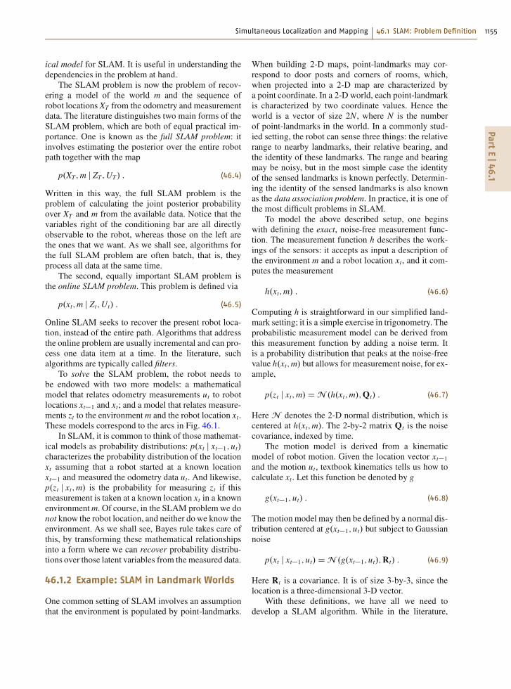
Figure 46.1 illustrates the variables involved in theSLAM problem. It shows the sequence of locations andsensor measurements, and the causal relationships be-tween these variables. This diagram represents a graph-

zt+1

x t+1x tx t –1

ztzt –1

ut+1utut –1

m

Fig. 46.1 Graphical model of the SLAM problem. Arcs in-dicate causal relationships, and shaded nodes are directlyobservable to the robot. In SLAM, the robot seeks to re-cover the unobservable variables

Simultaneous Localization and Mapping 46.1 SLAM: Problem Definition 1155Part

E|46.1

ical model for SLAM. It is useful in understanding thedependencies in the problem at hand.

The SLAM problem is now the problem of recov-ering a model of the world m and the sequence ofrobot locations XT from the odometry and measurementdata. The literature distinguishes two main forms of theSLAM problem, which are both of equal practical im-portance. One is known as the full SLAM problem: itinvolves estimating the posterior over the entire robotpath together with the map

p.XT ;m j ZT ;UT / : (46.4)

Written in this way, the full SLAM problem is theproblem of calculating the joint posterior probabilityover XT and m from the available data. Notice that thevariables right of the conditioning bar are all directlyobservable to the robot, whereas those on the left arethe ones that we want. As we shall see, algorithms forthe full SLAM problem are often batch, that is, theyprocess all data at the same time.

The second, equally important SLAM problem isthe online SLAM problem. This problem is defined via

p.xt;m j Zt;Ut/ : (46.5)

Online SLAM seeks to recover the present robot loca-tion, instead of the entire path. Algorithms that addressthe online problem are usually incremental and can pro-cess one data item at a time. In the literature, suchalgorithms are typically called filters.

To solve the SLAM problem, the robot needs tobe endowed with two more models: a mathematicalmodel that relates odometry measurements ut to robotlocations xt�1 and xt; and a model that relates measure-ments zt to the environmentm and the robot location xt.These models correspond to the arcs in Fig. 46.1.

In SLAM, it is common to think of those mathemat-ical models as probability distributions: p.xt j xt�1; ut/characterizes the probability distribution of the locationxt assuming that a robot started at a known locationxt�1 and measured the odometry data ut. And likewise,p.zt j xt;m/ is the probability for measuring zt if thismeasurement is taken at a known location xt in a knownenvironmentm. Of course, in the SLAM problemwe donot know the robot location, and neither do we know theenvironment. As we shall see, Bayes rule takes care ofthis, by transforming these mathematical relationshipsinto a form where we can recover probability distribu-tions over those latent variables from the measured data.

46.1.2 Example: SLAM in Landmark Worlds

One common setting of SLAM involves an assumptionthat the environment is populated by point-landmarks.

When building 2-D maps, point-landmarks may cor-respond to door posts and corners of rooms, which,when projected into a 2-D map are characterized bya point coordinate. In a 2-D world, each point-landmarkis characterized by two coordinate values. Hence theworld is a vector of size 2N, where N is the numberof point-landmarks in the world. In a commonly stud-ied setting, the robot can sense three things: the relativerange to nearby landmarks, their relative bearing, andthe identity of these landmarks. The range and bearingmay be noisy, but in the most simple case the identityof the sensed landmarks is known perfectly. Determin-ing the identity of the sensed landmarks is also knownas the data association problem. In practice, it is one ofthe most difficult problems in SLAM.

To model the above described setup, one beginswith defining the exact, noise-free measurement func-tion. The measurement function h describes the work-ings of the sensors: it accepts as input a description ofthe environment m and a robot location xt, and it com-putes the measurement

h.xt;m/ : (46.6)

Computing h is straightforward in our simplified land-mark setting; it is a simple exercise in trigonometry. Theprobabilistic measurement model can be derived fromthis measurement function by adding a noise term. Itis a probability distribution that peaks at the noise-freevalue h.xt;m/ but allows for measurement noise, for ex-ample,

p.zt j xt;m/DN .h.xt;m/;Qt/ : (46.7)

Here N denotes the 2-D normal distribution, which iscentered at h.xt;m/. The 2-by-2 matrix Qt is the noisecovariance, indexed by time.

The motion model is derived from a kinematicmodel of robot motion. Given the location vector xt�1

and the motion ut, textbook kinematics tells us how tocalculate xt. Let this function be denoted by g

g.xt�1; ut/ : (46.8)

The motion model may then be defined by a normal dis-tribution centered at g.xt�1; ut/ but subject to Gaussiannoise

p.xt j xt�1; ut/DN .g.xt�1; ut/;Rt/ : (46.9)

Here Rt is a covariance. It is of size 3-by-3, since thelocation is a three-dimensional 3-D vector.

With these definitions, we have all we need todevelop a SLAM algorithm. While in the literature,

PartE|46.1


point-landmark problems with range-bearing sensingare by far the most studied, SLAM algorithms are notconfined to landmark worlds. But no matter what themap representation and the sensor modality, any SLAMalgorithm needs a similarly crisp definition of the fea-tures in m, the measurement model p.zt j xt;m/, and themotion model p.xt j xt�1; ut/. Note that none of thosedistributions has to be restricted to Gaussian noise asdone in the example above.

46.1.3 Taxonomy of the SLAM Problem

SLAM problems are distinguished along a number ofdifferent dimensions. Most important research papersidentify the type of problems addressed by making theunderlying assumptions explicit. We already encoun-tered one such distinction: full versus online. Othercommon distinctions are as follows:

Volumetric Versus Feature-BasedIn volumetric SLAM, the map is sampled at a resolutionhigh enough to allow for photo-realistic reconstructionof the environment. The map m in volumetric SLAMis usually quite high-dimensional, with the result thatthe computation can be quite involved. Feature-basedSLAM extracts sparse features from the sensor stream.The map is then only comprised of features. Ourpoint-landmark example is an instance of feature-basedSLAM. Feature-based SLAM techniques tend to bemore efficient, but their results may be inferior to volu-metric SLAM due to the fact that the extraction of fea-tures discards information in the sensor measurements.

Topological Versus MetricSomemapping techniques recover only a qualitative de-scription of the environment, which characterizes therelation of basic locations. Such methods are known astopological. A topological map might be defined overa set of distinct places and a set of qualitative rela-tions between these places (e.g., place A is adjacent toplace B). Metric SLAM methods provide metric infor-mation between the relation of such places. In recentyears, topological methods have fallen out of fashion,despite ample evidence that humans often use topolog-ical information for navigation.

Known Versus Unknown CorrespondenceThe correspondence problem is the problem of relat-ing the identity of sensed things to other sensed things.In the landmark example above, we assumed that theidentity of landmarks is known. Some SLAM algo-rithms make such an assumption, others do not. Theones that do not provide special mechanisms for es-timating the correspondence of measured features to

previously observed landmarks in the map. The prob-lem of estimating the correspondence is known as dataassociation problem. It is one of the most difficult prob-lems in SLAM.

Static Versus DynamicStatic SLAM algorithms assume that the environmentdoes not change over time. Dynamic methods allowfor changes in the environment. The vast literature onSLAM assumes static environments. Dynamic effectsare often treated just as measurement outliers. Meth-ods that reason about motion in the environment aremore involved, but they tend to be more robust in mostapplications.

Small Versus Large UncertaintySLAM problems are distinguished by the degree oflocation uncertainty that they can handle. The most sim-ple SLAM algorithms allow only for small errors inthe location estimate. They are good for situations inwhich a robot goes down a path that does not intersectitself, and then returns along the same path. In manyenvironments it is possible to reach the same locationfrom multiple directions. Here the robot may accruea large amount of uncertainty. This problem is knownas the loop closing problem. When closing a loop, theuncertainty may be large. The ability to close loops isa key characteristic of modern-day SLAM algorithms.The uncertainty can be reduced if the robot can senseinformation about its position in some absolute coor-dinate frame, e.g., through the use of a satellite-basedglobal positioning system (GPS) receiver.

Active Versus PassiveIn passive SLAM algorithms, some other entity controlsthe robot, and the SLAM algorithm is purely observing.The vast majority of algorithms are of this type; theygive the robot designer the freedom to implement ar-bitrary motion controllers, and pursue arbitrary motionobjectives. In active SLAM, the robot actively exploresits environment in the pursuit of an accurate map. Ac-tive SLAM methods tend to yield more accurate mapsin less time, but they constrain the robot motion. Thereexist hybrid techniques in which the SLAM algorithmcontrols only the pointing direction of the robot’s sen-sors, but not the motion direction.

Single-Robot Versus Multi-RobotMost SLAM problems are defined for a single robotplatform, although recently the problem of multi-robot exploration has gained in popularity. Multi-robotSLAM problems come in many flavors. In some, robotsget to observe each other, in others, robots are told theirrelative initial locations. Multirobot SLAM problems

Simultaneous Localization and Mapping 46.2 The Three Main SLAM Paradigms 1157Part

E|46.2

are also distinguished by the type of communication al-lowed between the different robots. In some, the robotscan communicate with no latency and infinite band-width. More realistic are setups in which only nearbyrobots can communicate, and the communication issubject to latency and bandwidth limitations.

Any-Time and Any-SpaceRobots that do all computations onboard have limitedresources in memory and computation power. Any-time and any-space SLAM systems are an alternative

to traditional methods. They enable the robot to com-pute a solution given the resource constraints of thesystem. The more resources available, the better thesolution.

As this taxonomy suggests, there exists a flurry ofSLAM algorithms. Most modern-day conferences ded-icate multiple sessions to SLAM. This chapter focuseson the very basic SLAM setup. In particular it assumesa static environment with a single robot. Extensions arediscussed towards the end of this chapter, in which therelevant literature is discussed.

46.2 The Three Main SLAM Paradigms

This section reviews three basic SLAM paradigms,from which most others are derived. The first, known asEKF SLAM, is in robotics historically the earliest buthas become less popular due to its limiting computa-tional properties and issues resulting from performingsingle linearizations only. The second approach usesnonparametric statistical filtering techniques known asparticle filters. It is a popular method for online SLAMand provides a perspective on addressing the data asso-ciation problem in SLAM. The third paradigm is basedon graphical representations and successfully appliessparse nonlinear optimization methods to the SLAMproblem. It is the main paradigm for solving the fullSLAM problem and recently also incremental tech-niques are available.

46.2.1 Extended Kalman Filters

Historically, the EKF formulation of SLAM is the earli-est, and perhaps the most influential, SLAM algorithm.EKF SLAM was introduced in [46.10, 11] and [46.12,13], which were the first papers to propose the use ofa single state vector to estimate the locations of therobot and a set of features in the environment, with anassociated error covariance matrix representing the un-certainty in these estimates, including the correlationsbetween the vehicle and feature state estimates. As therobot moves through its environment taking measure-ments, the system state vector and covariance matrixare updated using the extended Kalman filter [46.14,15]. As new features are observed, new states are addedto the system state vector; the size of the system covari-ance matrix grows quadratically.

This approach assumes a metrical, feature-basedenvironmental representation, in which objects can beeffectively represented as points in an appropriate pa-rameter space. The position of the robot and the loca-tions of features form a network of uncertain spatialrelationships. The development of appropriate repre-

sentations is a critical issue in SLAM, and intimatelyrelated to the topics of sensing and world modeling dis-cussed in Chap. 36 and in Part C.

The EKF algorithm represents the robot estimate bya multivariate Gaussian

p.xt;m j Zt;Ut/DN .�t;† t/ : (46.10)

The high-dimensional vector �t contains the robot’sbest estimate of its own current location xt and thelocation of the features in the environment. In ourpoint-landmark example, the dimension of �t would be3C 2N, since we need three variables to represent therobot location and 2N variables for the N landmarks inthe map.

The matrix † t is the covariance of the robot’s as-sessment of its expected error in the guess �t. Thematrix † t is of size .3C 2N/� .3C 2N/ and it is pos-itive semi-definite. In SLAM, this matrix is usuallydense. The off-diagonal elements capture the correla-tions in the estimates of different variables. Nonzerocorrelations come along because the robot’s location isuncertain, and as a result the locations of the landmarksin the maps are uncertain.

The EKF SLAM algorithm is easily derived for ourpoint-landmark example. Suppose, for a moment, themotion function g and the measurement function hwerelinear in their arguments. Then, the vanilla Kalman fil-ter, as described in any textbook on Kalman filtering,would be applicable. EKF SLAM linearizes the func-tions g and h using Taylor series expansion. In its mostbasic form and in the absence of any data associationproblems, EKF SLAM is basically the application ofthe EKF to the online SLAM problem.

Figure 46.2 illustrates the EKF SLAM algorithm foran artificial example. The robot navigates from a startpose that serves as the origin of its coordinate system.As it moves, its own pose uncertainty increases, as in-dicated by uncertainty ellipses of growing diameter. It

http://dx.doi.org/10.1007/978-3-319-32552-1_36

PartE|46.2


a) b)

c) d)

Fig.46.2a–d EKF applied to theonline SLAM problem. The robot’spath is a dotted line, and its estimatesof its own position are shaded ellipses.Eight distinguishable landmarks ofunknown location are shown as smalldots, and their location estimates areshown as white ellipses. In (a–c)the robot’s positional uncertainty isincreasing, as is its uncertainty aboutthe landmarks it encounters. In (d) therobot senses the first landmark again,and the uncertainty of all landmarksdecreases, as does the uncertaintyof its current pose (image courtesyof Michael Montemerlo, StanfordUniversity)

also senses nearby landmarks and maps them with anuncertainty that combines the fixed measurement uncer-tainty with the increasing pose uncertainty. As a result,the uncertainty in the landmark locations grows overtime. The interesting transition happens in Fig. 46.2d:Here the robot observes the landmark it saw in the verybeginning of mapping, and whose location is relativelywell known. Through this observation, the robot’s poseerror is reduced, as indicated in Fig. 46.2d – noticethe very small error ellipse for the final robot pose.This observation also reduces the uncertainty for otherlandmarks in the map. This phenomenon arises froma correlation that is expressed in the covariance matrixof the Gaussian posterior. Since most of the uncertaintyin earlier landmark estimates is caused by the robotpose, and since this very uncertainty persists over time,the location estimates of those landmarks are correlated.When gaining information on the robot’s pose, this in-formation spreads to previously observed landmarks.This effect is probably the most important characteristicof the SLAM posterior [46.16]. Information that helpslocalize the robot is propagated through the map, and asa result improves the localization of other landmarks inthe map.

With a few adaptations, EKF SLAM can also be ap-plied in the presence of uncertain data association. Ifthe identity of observed features is unknown, the basic

EKF idea becomes inapplicable. The solution here isto reason about the most likely data association whena landmark is observed. This is usually done basedon proximity: which of the landmarks in the map cor-responds most likely to the landmark just observed?The proximity calculation considers the measurementnoise and the actual uncertainty in the poster estimate,and the metric used in this calculation is known asa Mahalanobis distance, which is a weighted quadraticdistance. To minimize the chances of false data asso-ciations, many implementations use visible features todistinguish individual landmarks and associate groupsof landmarks observed simultaneously [46.17, 18], al-though distinct features can also be computed fromlaser data [46.19, 20]. Typical implementations alsomaintain a provisional landmark list and only addlandmarks to the internal map when they have beenobserved sufficiently frequently [46.16, 21]. With anappropriate landmark definition and careful implemen-tation of the data association step, EKF SLAM has beenapplied successfully in a wide range of environments,using airborne, underwater, indoor, and various otherplatforms.

The basic formulation of EKF SLAM assumes thatthe location of features in the map is fully observablefrom a single position of the robot. The method hasbeen extended to situations with partial observability,


E|46.2

with range-only [46.22] or angle-only [46.23, 24] mea-surements. The technique has also been utilized usinga feature-less representation, in which the state consistsof current and past robot poses, and measurements takethe form of constraints between the poses (derived forexample from laser scan matching or from camera mea-surements) [46.25, 26].

A key concern of the EKF approach to SLAMlies in the quadratic nature of the covariance matrix.A number of researchers have proposed extensions tothe EKF SLAM algorithms that achieve scalability, forexample through submap decomposition [46.27–30].A related family of approaches [46.31–34] employs theExtended Information Filter, which operates on the in-verse of the covariance matrix. A key insight is thatwhereas the EKF covariance is densely populated, theinformation matrix is sparse when the full robot tra-jectory is maintained, leading to the development ofefficient algorithms and providing a conceptual linkto the pose graph optimization methods described inSect. 46.2.3.

The issues of consistency and convergence inEKF SLAM have been investigated in [46.35, 36].Observability-based rules for designing consistent EKFSLAM estimators are presented in [46.37].

46.2.2 Particle Methods

The second principal SLAM paradigm is based on par-ticle filters. Particle filters can be traced back to [46.38],but they have become popular only in the last twodecades. Particle filters represent a posterior througha set of particles. For the novice in SLAM, each par-ticle is best thought as a concrete guess as to whatthe true value of the state may be. By collecting manysuch guesses into a set of guesses, or set of particles,the particle filter approximates the posterior distribu-tion. Under mild conditions, the particle filter has beenshown to approach the true posterior as the particle setsize goes to infinity. It is also a nonparametric repre-sentation that represents multimodal distributions withease.

The key problem with the particle filter in the con-text of SLAM is that the space of maps and robot pathsis huge. Suppose we have a map with 100 features. Howmany particles would it take to populate that space?In fact, particle filters scale exponentially with the di-mension of the underlying state space. Three or fourdimensions are thus acceptable, but 100 dimensions aregenerally not.

The trick to make particle filters amenable to theSLAM problem goes back to [46.39, 40] and is knownas Rao–Blackwellization. It has been introduced intothe SLAM literature in [46.41], followed by [46.42],

who coined the name fastSLAM (fast simultaneous lo-calization and mapping). Let us first explain the basicFastSLAM algorithm on the simplified point-landmarkexample, and then discuss the justification for this ap-proach.

At any point in time, FastSLAM maintains K parti-cles of the type

XŒk�t ;�

Œk�t;1; : : : ;�

Œk�t;N ;†

Œk�t;1; : : : ;†

Œk�t;N : (46.11)

Here Œk� is the index of the sample. This expressionstates that a particle contains:

� A sample path XŒk�t , and

� A set of N 2-D Gaussians with means �Œk�t;n and

variances †Œk�t;n), one for each landmark in the en-

vironment.

Here n is the index of the landmark (with 1 nN). From that it follows that K particles possess K pathsamples. It also possessesKN Gaussians, each of whichmodels exactly one landmark for one of the particles.

Initializing FastSLAM is simple: just set each parti-cle’s robot location to the starting coordinates, typically.0; 0; 0/T, and zero the map. The particle update thenproceeds as follows:

� When an odometry reading is received, new loca-tion variables are generated stochastically, one foreach of the particles. The distribution for generat-ing those location particles is based on the motionmodel

xŒk�t p.xt j xŒk�t�1; ut/ : (46.12)

Here xŒk�t�1 is the previous location, which is partof the particle. This probabilistic sampling step iseasily implemented for any robot whose kinematicscan be computed.� When a measurement zt is received, two things hap-pen: first, FastSLAM computes for each particle theprobability of the new measurement zt. Let the in-dex of the sensed landmark be n. Then the desiredprobability is defined as follows

w Œk�t DN .zt j xŒk�t ;�Œk�

t;n;†Œk�t;n/ : (46.13)

The factor w Œk�t is called the importance weight,

since it measures how important the particle is inthe light of the new sensor measurement. As before,N denotes the normal distribution, but this time itis calculated for a specific value, zt. The importanceweights of all particles are then normalized so thatthey sum to 1.Next, FastSLAM draws with replacement from theset of existing particles a set of new particles. Theprobability of drawing a particle is its normalized

PartE|46.2


importance weight. This step is called resampling.The intuition behind resampling is that particlesfor which the measurement is more plausible havea higher chance of surviving the resampling pro-cess.Finally, FastSLAM updates for the new particle setthe mean �

Œk�t;n and covariance †Œk�

t;n, based on themeasurement zt. This update follows the standardEKF update rules – note that the extended Kalmanfilters maintained in FastSLAM are, in contrast toEKF SLAM, all low-dimensional (typically 2-D).

This all may sound complex, but FastSLAM isquite easy to implement. Sampling from the motionmodel usually involves simple kinematic calculations.Computing the importance of a measurement is oftenstraightforward too, especially for Gaussian measure-ment noise. And updating a low-dimensional particlefilter is also not complicated.

FastSLAM has been shown to approximate the fullSLAM posterior. The derivation of FastSLAM exploitsthree techniques: Rao–Blackwellization, conditional in-dependence, and resampling. Rao–Blackwellization isthe following concept. Suppose we would like to com-pute a probability distribution p.a;b/, where a and bare arbitrary random variables. The vanilla particle filterwould draw particles from the joint distributions, thatis, each particle would have a value for a and one for b.However, if the conditional p.b j a/ can be described inclosed form, it is equally legitimate to just draw parti-cles from p.a/, and attach to each particle a closed-formdescription of p.b j a/. This trick is known as Rao–

zt–1 zt+1

xt+1

zt

xt

ut–1 ut+1ut

xt–1

m1 m2

zt+2

xt+2

ut+2

m3

Fig. 46.3 The SLAM problem depicted as Bayes network graph.The robot moves from location xt�1 to location xtC2, driven bya sequence of controls. At each location xt it observes a nearbyfeature in the map mD fm1;m2;m3g. This graphical network illus-trates that the location variables separate the individual features inthe map from each other. If the locations are known, there remainsno other path involving variables whose value is not known, be-tween any two features in the map. This lack of a path renders theposterior of any two features in the map conditionally independent(given the locations)

Blackwellization, and it yields better results than sam-pling from the joint. FastSLAM applies this technique,in that it samples from the path posterior p.XŒk�

t j Ut;Zt/and represents the map p.m j XŒk�

t ;Ut;Zt/ in Gaussianform.

FastSLAM also breaks down the posterior overmaps (conditioned on paths) into sequences of low-dimensional Gaussians. The justification for this de-composition is subtle. It arises from a specific condi-tional independence assumption that is native to SLAM.Fig. 46.3 illustrates the concept graphically. In SLAM,knowledge of the robot path renders all landmark esti-mates independent. This is easily shown for the graph-ical network in Fig. 46.3: we find that if we removethe path variables from Fig. 46.3, then the landmarkvariables are all disconnected [46.43]. Thus, in SLAMany dependence between multiple landmark estimatesis mediated through the robot path. This subtle butimportant observation implies that even if we useda large, monolithic Gaussian for the entire map (oneper particle, of course), the off-diagonal element be-tween different landmarks would simply remain zero.It is therefore legitimate to implement the map moreefficiently, using N small Gaussians, one for each land-mark. This explains the efficient map representation inFastSLAM.

Figure 46.4 shows results for a point-feature prob-lem; here the point features are the centers of treetrunks as observed by an outdoor robot. The datasetused here is known as the Victoria Park dataset [46.44].Fig. 46.4a shows the path of the vehicle obtained byintegrating the vehicle controls, without perception. Ascan be seen, controls are a poor predictor of location forthis vehicle; after 30min of driving, the estimated po-sition of the vehicle is well over 100m away from itsGPS position.

The FastSLAM algorithm has a number of inter-esting properties. First, it solves both full and onlineSLAM problems. Each particle has a sample of an en-tire path but the actual update equation only uses themost recent pose. This makes FastSLAM a filter. Sec-ond, FastSLAM can maintain multiple data associationhypotheses. It is straightforward to make data associa-tion decisions on a per-particle basis, instead of havingto adopt the same hypothesis for the entire filter. Whilewe will not give any mathematical justification, wenote that the resulting FastSLAM algorithm can evendeal with unknown data association – something thatthe extended Kalman filter cannot claim. And third,FastSLAM can be implemented very efficiently usingadvanced tree methods to represent the map estimates,the update can be performed in time logarithmic in thesize of the map N, and linear in the number of parti-cles M.


E|46.2

a) b) c)Raw vehicle path FastSLAM (solid), GPS path (dashed) Path and map with aerial image

Fig. 46.4 (a) Vehicle path predicted by the odometry; (b) True path (dashed line) and FastSLAM 1.0 path (solid line);(c) Victoria Park results overlaid on aerial imagery with the GPS path in blue (dashed), average FastSLAM 1.0 path inyellow (solid), and estimated features as yellow dots (data and aerial image courtesy of José Guivant and Eduardo Nebot,Australian Centre for Field Robotics)

a) b)

Fig. 46.5 Occupancy grid map generated from laser range data and based on pure odometry (image courtesy of DirkHähnel, University of Freiburg)

FastSLAM has been extended in several ways. Oneset of variants are grid-based versions of FastSLAM,in which the Gaussians used to model point landmarksare replaced by an occupancy grid map [46.45–47]. Thevariant of [46.46] is illustrated in Fig. 46.5.

Figure 46.6 illustrates a simplified situation withthree particles just before closing a large loop. The threedifferent particles each stand for different paths, andthey also posses their own local maps. When the loopis closed importance resampling selects those particles

whose maps are most consistent with the measure-ment. A resulting large-scale map is shown in Fig. 46.5.Further extensions can be found in [46.48, 49], whosemethods are called DP-SLAM and operate on ances-try trees to provide efficient tree update methods forgrid-based maps. Related to that, approximations toFastSLAM in which particles share their maps havebeen proposed [46.50].

The works in [46.45, 47, 51] provide ways to in-corporate new observations into the location sampling

PartE|46.2


Map of particle 1 Map of particle 1 Map of particle 1

3 particles and their trajectories

Fig. 46.6 Application of the grid-based variant of the FastSLAM algorithm. Each particle carries its own map and theimportance weights of the particles are computed based on the likelihood of the measurements given the particle’s ownmap

process for landmarks and grid maps, based on priorwork in [46.52]. This leads to an improved samplingprocess

xŒk�t p.zt j mŒk�t�1; xt/ p.xt j xŒk�t�1; ut/

p.zt j mŒk�t�1; x

Œk�t�1; ut/

; (46.14)

which incorporates the odometry and the observationat the same time. Using an improved proposal dis-tribution leads to more accurately sampled locations.This in turn leads to more accurate maps and requiresa smaller number of particles compared to approachesusing the sampling process given in (46.12). This ex-tension makes FastSLAM and especially its grid-basedvariants robust tools for addressing the SLAM problem.

Finally, there are approaches that aim to overcomethe assumption that the observations show Gaussiancharacteristics. As shown in [46.47], there are sev-eral situations in which the model is nonGaussian andalso multimodal. A sum of Gaussians model on a per-particle bases, however, can be efficiently consideredin the particle filter and it eliminates this problem inpractice without introducing additional computationaldemands.

The so-far developed particle filters-based SLAMsystems suffer from two problems. First, the number ofsamples that are required to compute consistent mapsis often set manually by making an educated guess.The larger the uncertainty that the filter needs to rep-resent during mapping, the more critical becomes this

parameter. Second, nested loops combined with exten-sive re-visits of previously mapped areas can lead toparticle depletion, which in turn may prevent the systemfrom estimating a consistent map. Adaptive resamplingstrategies [46.45], particles sharing maps [46.50], or fil-ter backup approaches [46.53] improve the situation butcannot eliminate this problem in general.

46.2.3 Graph-BasedOptimization Techniques

A third family of algorithms solves the SLAM problemthrough nonlinear sparse optimization. They draw theirintuition from a graphical representation of the SLAMproblem and the first working solution in robotics wasproposed in [46.54]. The graph-based representationused here is closely related to a series of papers [46.55–64]. We note that most of the earlier techniques areoffline and address the full SLAM problem. In morerecent years, new incremental versions that effectivelyre-use the previously computed solution have been pro-posed such as [46.65–67].

The basic intuition of graph-based SLAM is a fol-lows. Landmarks and robot locations can be thought ofas nodes in a graph. Every consecutive pair of locationsxt�1; xt is tied together by an edge that represents theinformation conveyed by the odometry reading ut. Fur-ther edges exist between the nodes that correspond tolocations xt and landmarks mi, assuming that at time tthe robot sensed landmark i. Edges in this graph are


E|46.2

soft constraints. Relaxing these constraints yields therobot’s best estimate for the map and the full path.

The construction of the graph is illustrated inFig. 46.7. Suppose at time tD 1, the robot senseslandmark m1. This adds an arc in the (yet highly in-complete) graph between x1 and m1. When cachingthe edges in a matrix format (which happens to cor-respond to a quadratic equation defining the resultingconstraints), a value is added to the elements be-tween x1 and m1, as shown on the right hand side ofFig. 46.7a.

Now suppose the robot moves. The odometry read-ing u2 leads to an arc between nodes x1 and x2, asshown in Fig. 46.7b. Consecutive application of thesetwo basic steps leads to an graph of increasing size,as illustrated in Fig. 46.7c. Nevertheless this graph issparse, in that each node is only connected to a smallnumber of other nodes (assuming a sensor with limitedsensing range). The number of constraints in the graphis (at worst) linear in the time elapsed and in the num-ber of nodes in the graph.

m2

x2 x3 x4x1

m3m4m1

m4m3m2m1x4x3x2x1

x1

x2

x3

x4

m1

m2

m3

m4

x1

m1

m1x1

x1

m1

a)

c)

x2x1

m1

m1x2x1

x1

x2

m1

b)

Fig.46.7a–c Illustration of the graph construction. The (a)diagram shows the graph, the (b) the constraints in matrixform. (a) Observation ls landmark m1. (b) Robot motionfrom x1 to x2. (c) Several steps later

If we think of the graph as a spring-mass mod-el [46.60], computing the SLAM solution is equivalentto computing the state of minimal energy of this model.To see, we note that the graph corresponds to the log-posterior of the full SLAM problem (46.4)

log p.XT ;m j ZT ;UT / : (46.15)

Without derivation, we state that this logarithm is of theform

log p.XT ;m j ZT ;UT/

D constCXt

log p.xt j xt�1; ut/

CXt

log p.zt j xt;m/ ; (46.16)

assuming independence between the individual obser-vations and odometry readings. Each constraint of theform log p.xt j xt�1; ut/ is the result of exactly one robotmotion event, and it corresponds to an edge in the graph.Likewise, each constraint of the form log p.zt j xt;m/ isthe result of one sensor measurement, to which we canalso find a corresponding edge in the graph. The SLAMproblem is then simply to find the mode of this equa-tion, i. e.,

X�

T ;m� D argmax

XT ;mlog p.XT ;m j ZT ;UT/ : (46.17)

Without derivation, we note that under the Gaussiannoise assumptions, which was made in the point-landmark example, this expression resolves to the fol-lowing quadratic form

log p.XT ;m j ZT ;UT/D const

CXt

Œxt � g.xt�1; ut/�T R�1

t Œxt � g.xt�1; ut/�„ ƒ‚ …odometry reading

CXt

Œzt � h.xt;m/�T Q�1

t Œzt � h.xt;m/�„ ƒ‚ …feature observation

:

(46.18)

This quadratic form yields a sparse system of equationsand a number of efficient optimization techniques canbe applied. Common choices include direct methodssuch as sparse Cholesky and QR decomposition, or iter-ative ones such as gradient descent, conjugate gradient,and others. Most SLAM implementations rely on iter-atively linearizing the functions g and h, in which casethe objective in (46.18) becomes quadratic in all of itsvariables.

Extensions to support an effective correction oflarge-scale graphs are hierarchical methods. One of

PartE|46.2


the first is the ATLAS framework [46.25], which con-structs a two-level hierarchy combining a Kalman filterthat operates in the lower level and a global optimiza-tion at the higher level. Similar to that, HierarchicalSLAM [46.68] is a technique for using independentlocal maps, which are merged in case of re-visitinga place. A fully hierarchical approach has been pre-sented in [46.65]. It builds a multilevel pose-graph andemploys an incremental, lazy optimization scheme thatallows for optimizing large graphs and at the same timecan be executed at each step during mapping. An al-ternative hierarchical approach is [46.69], which recur-sively partitions the graph into multiple-level submapsusing the nested dissection algorithm.

When it comes to computing highly accurate envi-ronment reconstructions, approaches that do not onlyoptimize the poses of the robot but also each indi-vidual measurement of a dense sensor often providebetter results. In the spirit of bundle adjustment [46.4],approaches for laser scanners [46.70] and Kinect cam-eras [46.71] have been proposed.

The graphical paradigm can be extended to han-dle the data association problems as we can integrateadditional knowledge on data association into (46.18).Suppose some oracle informed us that landmarks mi

and mj in the map corresponded to one and the samephysical landmark in the world. Then, we can ei-ther remove mj from the graph and attach all adjacentedges to mi, or we can add a soft correspondence con-straint [46.72] of the form

.mj�mi/T � .mj�mi/ : (46.19)

Here � is 2-by-2 diagonal matrix whose coefficients de-termine the penalty for not assigning identical locationsto two landmarks (hence we want � to be large). Sincegraphical methods are usually used for the full SLAMproblem, the optimization can be interleaved with thesearch for the optimal data association.

Data association errors typically have a strong im-pact in the resulting map estimate. Even a small numberof wrong data associations is likely to result in incon-sistent map estimates. Recently, novel approaches havebeen proposed that are robust under a certain number offalse associations. For example, [46.73, 74] propose aniterative procedure that allows for disabling constraints,an action that is associated with a cost. A generalizationof this method introduced in [46.75] formulates [46.74]as a robust cost function also reducing the compu-tational requirements. Such approaches can deal witha significant number of false associations and still pro-vide high-quality maps. Consistency checks for loopclosure hypotheses can be found in other approachesas well, both in the front-end [46.76] and in the opti-

mizer [46.77]. There has also been an extension that candeal with multimodal constraints [46.78], proposinga max-mixture representation for maintaining efficiencyof the log likelihood optimizing in (46.16). As a resultof that, the multimodal extension has only little im-pact on the runtime and can easily be incorporated inmost optimizers. Also robust cost function are used forSLAM, for example pseudo Huber and several alterna-tives [46.75, 79–81].

Graphical SLAM methods have the advantage thatthey scale to much higher-dimensional maps than EKFSLAM, exploiting the sparsity of the graph. The keylimiting factor in EKF SLAM is the covariance matrix,which takes space (and update time) quadratic in thesize of the map. No such constraint exists in graphicalmethods. The update time of the graph is constant, andthe amount of memory required is linear (under somemild assumptions). A further advantage of graph-basedmethods over the EKF is their ability to constantly re-linearize the error function which often leads to betterresults. Performing the optimization can be expensive,however. Technically, finding the optimal data associa-tion is suspected to be an NP-hard problem, although inpractice the number of plausible assignments is usuallysmall. The continuous optimization of the log likeli-hood function in (46.18) depends among other thingson the number and size of loops in the map. Also theinitialization can have a strong impact on the result anda good initial guess can simplify the optimization sub-stantially [46.8, 82, 83].

We note that the graph-based paradigm is veryclosely linked to information theory, in that the soft con-straints constitute the information the robot has on theworld (in an information-theoretic sense [46.92]). Mostmethods in the field are offline and they optimize forthe entire robot path. If the robot path is long, the opti-mization may become cumbersome. Over the last fiveyears, however, incremental optimization techniqueshave been proposed that aim at providing a sufficientbut not necessarily perfect model of the environmentat every point in time. This allows a robot to makedecisions based on the current model, for example, todetermine exploration goals. In this context, incremen-tal variants [46.93, 94] of stochastic gradient descenttechniques [46.8, 91] have been proposed that estimatewhich part of the graph requires re-optimization givennew sensor data. Incremental methods [46.66, 79, 95] inthe smoothing and mapping framework can be executeat each step of the mapping process and achieve theperformance by variable ordering and selective relin-earization. As also evaluated in [46.96] for the SLAMproblem, variable ordering impacts the performance ofthe optimization. Others use hierarchical data struc-tures [46.89] and pose-graphs [46.97] combined with


E|46.2

Table 46.1 Recent open-source graph-based SLAM implementations

Name CommentDynamic covariancescaling (DCS) [46.75]

Optimization with a robust cost function for dealing with outliersIntegrated into g2o

g2o [46.80] Flexible and easily extendable optimization framework for SLAMComes with different optimization approaches and error functionsSupports external plugins

GTSAM2.1 [46.79] Flexible optimization framework for SLAM and SFMstructure from motionImplements direct and iterative optimization techniquesImplements smoothing and mapping (SAM), iSAM, and iSAM2Implements bundle adjustment for Visual SLAM and SFM

HOG-Man [46.65] Incremental optimization approach via hierarchical pose graphs and lazy optimizationRequires pose-graphs with full rank constraints

iSAM2 [46.66] General incremental nonlinear optimization with variable eliminationVariable re-ordering to retain sparsityOn-demand re-linearization of selected variables

KinFu (KinectFusionreimplemented)

Open source reimplementation of KinectFusion [46.84] within the point cloud library (PCL)Dense and highly accurate reconstruction using a Kinect cameraCurrently limited to medium sized rooms

MaxMixture [46.78] Optimization for multimodal constraints and outliersRobust to outliersPlugin for g2o

Parallel tracking andmapping (PTAM) [46.85]

System for tracking a hand-held monocular camera and observed featuresOperates on comparably small workspaces

RGBD-SLAM [46.86] Kinect-frontend for HOG-Man and g2oFairly standard combination of SURF matching and RANSAC

ScaViSLAM [46.87] SLAM system for stereo and Kinect-style camerasCombines local bundle adjustment with sparse global optimization for on-the-fly processing

SLAM6-D [46.88] SLAM system that operates on point clouds from 3-D laser dataApplies iterative closest point algorithm (ICP) and global relaxation

Sparse surface adjustment(SSA) [46.70, 71]

Optimizes robot poses and proximity sensor data jointlyProvides smooth surface estimatesAssumes a range sensor (e.g., laser scanner, Kinect, or similar)

TreeMap [46.89] Incremental optimization approachUpdate in O .logN/ timeProvides only a mean estimate

TORO [46.90] Optimization approach that extends stochastic gradient descent (SGD) [46.91]Robust under bad initial guessesRecovers quickly from large errors but slow convergence at minimumAssumes that constraints have roughly spherical covariance matricesProvides only a mean estimate

Vertigo [46.74] Switchable constraints for robust optimizationPlugin for g2o

a lazy optimization for on-the-fly mapping [46.65]. Asan alternative to global methods, relative optimizationapproaches [46.98] aim at computing locally consistentgeometric maps but only topological maps on the globalscale. Hybrid approaches [46.87] seek to combine thebest of both worlds.

There also exists a number of cross-overs that ma-nipulate the graph online so as to factor out pastrobot location variables. The resulting algorithms arefilters [46.25, 33, 99, 100], and they tend to be inti-mately related to information filter methods. Many ofthe original attempts to decompose EKF SLAM repre-sentations into smaller submaps to scale up are based

on motivations that are not dissimilar to the graphicalapproach [46.27, 28, 101].

Recently, researchers addressed the problem oflong-term operation and frequent revisits of alreadymapped terrain. To avoid densely connected pose-graphs that lead to slow convergence behavior, the robotcan switch between SLAM and localization, can mergenodes to avoid a growth of the graph [46.90, 102], orcan discard nodes or edges [46.32, 103–105].

Graphical and optimization-based SLAM algorithmare still subject of intense research and the paradigmscales to maps large numbers of nodes [46.25, 55, 57,59, 63–65, 89, 90, 106, 107]. Arguably, the graph-based

PartE|46.3


paradigm has generated some the largest SLAM mapsever built. Furthermore, the SLAM community startedto release flexible optimization frameworks and SLAMimplementations under open source licenses to sup-port further developments and to allow for efficientcomparisons, (Table 46.1). Especially the optimizationframeworks [46.66, 79, 80] are flexible and powerfulstate of the art tools for developing graph-based SLAMsystems. They can be either used as a black box or canbe easily extended though plugins.

46.2.4 Relation of Paradigms

The three paradigms just discussed cover the vast ma-jority of work in the field of SLAM. As discussed,EKF SLAM comes with a computational hurdle thatposes serious scaling limitations and the linearizationmay lead to inconsistent maps. The most promising ex-tensions of EKF SLAM are based on building localsubmaps; however, in many ways the resulting algo-rithms resemble the graph-based approach.

Particle filter methods sidestep some of the is-sues arising from the natural inter-feature correlationsin the map – which hindered the EKF. By samplingfrom robot poses, the individual landmarks in the map

become independent, and hence are decorrelated. Asa result, FastSLAM can represent the posterior bya sampled robot pose, and many local, independentGaussians for its landmarks. The particle representationoffers advantages for SLAM as it allows for compu-tationally efficient updates and for sampling over dataassociations. On the negative side, the number of neces-sary particles can grow very large, especially for robotsseeking to map multiple nested loops.

Graph-based methods address the full SLAM prob-lem, hence are in the standard formulation not online.They draw their intuition form the fact that SLAMcan be modeled by a sparse graph of soft constraints,where each constraint either corresponds to a motion ora measurement event. Due to the availability of highlyefficient optimization methods for sparse nonlinear op-timization problems, graph-based SLAM has becomethe method of choice for building large-scale maps.Recent developments have brought up several graph-based methods for incremental map building that canbe executed at every time step during navigation. Dataassociation search can be incorporated into the basicmathematical framework and different approaches thatare even robust under wrong data associations are avail-able today.

46.3 Visual and RGB-D SLAM

A popular and important topic in recent years has beenVisual SLAM – the challenge of building maps andtracking the robot pose in full 6-DOF using data fromcameras [46.108] or RGB-D (Kinect) sensors [46.86,109]. Visual sensors offer a wealth of information thatenables the construction of rich 3-D models of theworld. They also enable difficult issues such as loop-closing to be addressed in novel ways using appearanceinformation [46.110]. Visual SLAM is anticipated tobe a critical area for future research in perception forrobotics, as we seek to develop low-cost systems thatare capably of intelligent physical interaction with theworld.

Attempting SLAM with monocular, stereo, om-nidirectional, or RGB-D cameras raises the level-of-difficulty of many of the SLAM components, suchas data association and computational efficiency, de-scribed above. A key challenge is robustness. Manyvisual SLAM applications of interest, such as aug-mented reality [46.85], entail handheld camera motions,which present greater difficulties for state estimation,in comparison to the motion of a wheeled robot acrossa flat floor.

Visual navigation and mapping was a key early goalin the mobile robotics community [46.111, 112], but

early approaches were hampered by the lack of suffi-cient computational resources to handle massive videodata streams. Early approaches were typically basedon extended Kalman filters [46.113–116], but did notcompute the full covariance for the feature poses andcamera trajectory, resulting in a loss of consistency.Visual SLAM is closely related to the structure frommotion (SFM) problem in computer vision [46.4, 5].Historically, SFM was primarily concerned with off-line batch processing, whereas SLAM seeks to achievea solution for online operation, suitable for closed-loopinteraction of a robot or user with its environment. Incomparison to laser scanners, cameras provide a fire hy-drant of information, making online processing nearlyimpossible until recent increases in computation havebecome available.

Davison was an early pioneer in developing com-plete visual SLAM systems, initially using a real-timeactive stereo head [46.121] that tracked distinctive vi-sual features with a full covariance EKF approach. Sub-sequent work developed the first real-time SLAM sys-tem that operated with a single freely moving cameraas the only data source [46.23, 122]. This system couldbuild sparse, room-size maps of indoor scenes at 30Hzframe-rate in real-time, a notable historical achievement

Simultaneous Localization and Mapping 46.3 Visual and RGB-D SLAM 1167Part

E|46.3

a) b)

–50 0 50 100 150 200 250 –50 0 50 100 150 200 25050

0

– 50

– 100

– 150

– 200 – 140

– 120

– 100

– 80

– 60

– 40

– 20

0

20

y (m) y (m)

x (m

)Fig. 46.8 (a) A 2-km path and 50 000 frames estimated for the New College Dataset (after [46.117]) using relativebundle adjustment (after [46.98]). (b) the relative bundle adjustment solution is easily improved by taking FAB-MAP(after [46.118]) loop-closures into account – this is achieved without global optimization (after [46.119]). Sibley et al.advocate that relative metric accuracy and topological consistency are the requirements for autonomous navigation,and these are better achieved using a relative manifold representation instead of using a conventional single Euclideanrepresentation [46.120]

a) b)

Fig. 46.9 (a) 3-D Model and (b) close-up view of a corridor environment in the Paul G. Allen building at University ofWashington built from Kinect data (after [46.109]; image courtesy of Peter Henry, University of Washington)

in visual SLAM research. A difficulty encountered withinitial monocular SLAM [46.23] was coping with theinitialization of points that were far away from the cam-era, due to nonGaussian distributions of such feature lo-cations resulting from poor depth information. This lim-itation was overcome in [46.24], introducing an inversedepth parameterization for monocular SLAM, a keydevelopment for enabling a unified treatment of initial-ization and tracking of visual features in real-time.

A milestone in creating robust visual SLAM sys-tems was the introduction of keyframes in paralleltracking and mapping (PTAM) [46.85], which sep-arated the tasks of keyframe mapping and localiza-tion into parallel threads, improving robustness andperformance for online processing. Keyframes arenow a mainstream concept for complexity reduc-tion in visual SLAM systems. Related approachesusing keyframes include [46.87, 123–126]. The work

PartE|46.3


in [46.108] analyzes the tradeoffs between filtering andkeyframe-based bundle adjustment in visual SLAM,and concluded that keyframe bundle adjustment outper-forms filtering, as it provides the most accuracy per unitof computing time.

As pointed out by Davison and other researchers,an appealing aspect of visual SLAM is that camerameasurements can provide odometry information, andindeed visual odometry is a key component of modernSLAM systems [46.127]. Here, [46.128] and [46.129]provide an extensive tutorial of techniques for visualodometry, including feature detection, feature match-ing, outlier rejection, and constraint estimation, andtrajectory optimization. Finally, a publicly available vi-sual odometry library [46.130] that is optimized forefficient operation on small unmanned aerial vehiclesis available today.

Visual information offers a tremendous source of in-formation for loop closing, not present in the canonical2-D laser SLAM systems developed in the early 2000s.The work in [46.110] was one of the first to employtechniques for visual object recognition [46.131] to lo-cation recognition. More recently FAB-MAP [46.118,132] has demonstrated appearance-only place recogni-tion at large scale, mapping trajectories with a lengthof 1000km. Combining a bag-of-features approachwith a probabilistic place model and Chow–Liu treeinference leads to place recognition that is robustagainst perceptual aliasing while remaining compu-tationally efficient. Other work on place recognitionincludes [46.133], which combines bag-of-words loopclosing with tests of geometrical consistency based onconditional random fields (Fig. 46.8).

The techniques described above have formed thebasis for a number of notable large-scale SLAM sys-tems developed in recent years. A 2008 special is-sue of the IEEE Transactions on Robotics providesa good snapshot of recent state-of-the-art SLAM tech-niques [46.135]. Other notable recent examples in-clude [46.98, 119, 126, 136–138]. The idea of employ-ing relative bundle adjustment [46.98] to compute a fullmaximum likelihood solution in an online fashion,even for loop closures, by employing a manifold rep-resentation that does not attempt to enforce Euclideanconstraints results in maps that can be computed athigh frame rate (see also Fig. 46.8). Finally, view-basedmapping systems [46.126, 136, 137] aim at large-scaleand/or life-long visual mapping based on the posegraph optimization techniques described above in Sec-tion 46.2.3.

Several compelling 3-D mapping and localizationhave been created in recent years with RGB-D (Kinect)sensors. The combination of direct range measurementswith dense visual imagery can enable dramatic im-

provements in mapping and navigation systems for in-door environments. State-of-the-art RGB-D SLAM sys-tems include [46.109] and [46.86]. Figure 46.9 showsexamples of the output of these systems.

Other researchers aim at exploiting the surfaceproperties of scanned environments to correct for sen-

a)

b)

c)

Fig.46.10a–c Results obtained with KinectFusion (af-ter [46.134]). (a) A local scene as a normal map and (b) asa Phong-shaded rendering. The (c) image depicts a largerscene (image courtesy of Richard Newcombe, ImperialCollege London)

Simultaneous Localization and Mapping 46.4 Conclusion and Future Challenges 1169Part

E|46.4

Fig. 46.11 Spatially ex-tended KinectFusion outputproduced in real-time withKintinuous (after [46.139])

sor noise of range sensors such as the Kinect [46.71].They jointly optimize the poses of the sensor andthe positions of the surface points measured and it-eratively refine the structure of the error functionby recomputing the data associations after each opti-mization, resulting in accurate smooth models of theenvironment.

An emerging area for future research is the de-velopment of fully dense processing methods thatexploit recent advances in commodity graphical pro-cessing unit (GPU) technology. Kinect-based densetracking and mapping, a fully-dense method for small-scale visual tracking and reconstruction is describedin [46.140]. Dense modeling and tracking are achieved

via highly parallelized operations on commodity GPUhardware to yield a system that outperforms previ-ous methods such as PTAM for challenging cameratrajectories. Dense methods offer an interesting per-spective from which to address long-standing problems,such as visual odometry, from a fresh perspective,without requiring explicit feature detection and match-ing [46.141]. KinectFusion [46.84, 134] is a dense mod-eling system that tracks the 3-D pose of a handheldKinect while concurrently reconstructing high-qualityscene 3-D models in real-time. See Fig. 46.10 for anexample. KinectFusion has been applied to spatially ex-tended environments in [46.139, 142]. An example isshown in Fig. 46.11.

46.4 Conclusion and Future Challenges

This chapter has provided an introduction into SLAM,which is defined as the problem faced by a mobileplatform roaming an unknown environment, and seek-ing to localize itself while concurrently building a mapof the environment. The chapter discussed three mainparadigms in SLAM, which are based on the ex-tended Kalman filter, particle filters, and graph-basedsparse optimization techniques, and then described re-cent progress in Visual/Kinect SLAM.

The following references provide an in-depth tuto-rial on SLAM and much greater depth of coverage onthe details of popular SLAM algorithms. Furthermore,several implementations of popular SLAM systems, in-cluding most of the approaches listed in Table 46.1,can be found in online resources such as http://www.openslam.org or in the references [46.6, 9, 21, 62].

The considerable progress in SLAM in the pastdecade is beyond doubt. The core state estimation at

http://www.openslam.org

http://www.openslam.org

PartE|46


the heart of SLAM is now quite well understood,and a number of impressive implementations havebeen developed, including several widely used opensource software implementations and some commer-cial projects. None-the-less, a number of open researchchallenges remain for the general problem of roboticmapping in complex and dynamic environments overextended periods of time, including robots sharing, ex-tending, and revising previously built models, efficientfailure recovery, zero user intervention, and operationon resource-constrained systems. Another exciting areafor the future is the further development of fully densevisual mapping systems exploiting the latest advancesin GPU hardware development.

An ultimate goal is to realize the challenge of per-sistent navigation and mapping – the capability fora robot to perform SLAM robustly for days, weeks,or months at a time with minimal human supervi-sion, in complex and dynamic environments. Takingthe limit as t!1 poses difficult challenges to mostcurrent algorithms; in fact, most robot mapping andnavigation algorithms are doomed to fail with thepassage of time, as errors inevitably accrue. Despiterecent encouraging solutions [46.102, 105], more re-search is needed for techniques that can recover frommistakes and enable robots to deal with changes inthe environment and enabling a long-term autonomousexistence.

Video-References

VIDEO 439 Deformation-based loop closure for Dense RGB-D SLAMavailable from http://handbookofrobotics.org/view-chapter/46/videodetails/439

VIDEO 440 Large-scale SLAM using the Atlas frameworkavailable from http://handbookofrobotics.org/view-chapter/46/videodetails/440

VIDEO 441 Graph-based SLAMavailable from http://handbookofrobotics.org/view-chapter/46/videodetails/441





VIDEO 446 Graph-based SLAM using TOROavailable from http://handbookofrobotics.org/view-chapter/46/videodetails/446

VIDEO 447 Sparse pose adjustmentavailable from http://handbookofrobotics.org/view-chapter/46/videodetails/447

VIDEO 449 Pose graph compression for laser-based SLAMavailable from http://handbookofrobotics.org/view-chapter/46/videodetails/449



VIDEO 452 DTAM: Dense tracking and mapping in real-timeavailable from http://handbookofrobotics.org/view-chapter/46/videodetails/452

VIDEO 453 MonoSLAM: Real-time single camera SLAMavailable from http://handbookofrobotics.org/view-chapter/46/videodetails/453

VIDEO 454 SLAM++: Simultaneous localisation and mapping at the level of objectsavailable from http://handbookofrobotics.org/view-chapter/46/videodetails/454

VIDEO 455 Extended Kalman filter SLAMavailable from http://handbookofrobotics.org/view-chapter/46/videodetails/455

http://handbookofrobotics.org/view-chapter/46/videodetails/439
































Simultaneous Localization and Mapping References 1171Part

E|46

References

46.1 C.F. Gauss: Theoria Motus Corporum Coelestium(Theory of the Motion of the Heavenly Bodies Mov-ing about the Sun in Conic Sections) (Perthes andBessen, Hamburg 1809), Republished in 1857 andby Dover in 1963

46.2 D.C. Brown: The bundle adjustment – Progressand prospects, Int. Arch. Photogramm. 21(3), 3:3–3:35 (1976)

46.3 G. Konecny: Geoinformation: Remote Sensing,Photogrammetry and Geographical InformationSystems (Taylor Francis, London 2002)

46.4 B. Triggs, P. McLauchlan, R. Hartley, A. Fitzgibbon:Bundle adjustment – A modern synthesis, Lect.Notes Comput. Sci. 62, 298–372 (2000)

46.5 R. Hartley, A. Zisserman: Multiple View Geometryin Computer Vision (Cambridge Univ. Press, Cam-bridge 2003)

46.6 T. Bailey, H.F. Durrant-Whyte: Simultaneous lo-calisation and mapping (SLAM): Part II, RoboticsAutom. Mag. 13(3), 108–117 (2006)

46.7 H.F. Durrant-Whyte, T. Bailey: Simultaneous lo-calisation and mapping (SLAM): Part I, RoboticsAutom. Mag. 13(2), 99–110 (2006)

46.8 G. Grisetti, C. Stachniss, W. Burgard: Nonlinearconstraint network optimization for efficient maplearning, IEEE Trans. Intell. Transp. Syst. 10(3),428–439 (2009)

46.9 S. Thrun, W. Burgard, D. Fox: ProbabilisticRobotics (MIT Press, Cambridge, 2005)

46.10 R. Smith, M. Self, P. Cheeseman: A stochasticmap for uncertain spatial relationships, Proc. Int.Symp. Robotics Res. (ISRR) (MIT Press, Cambridge1988) pp. 467–474

46.11 R. Smith, M. Self, P. Cheeseman: Estimating un-certain spatial relationships in robotics. In: Au-tonomous Robot Vehicles, ed. by I.J. Cox, G.T. Wil-fong (Springer Verlag, Berlin, Heidelberg 1990)pp. 167–193

46.12 P. Moutarlier, R. Chatila: Stochastic multisensorydata fusion for mobile robot location and envi-ronment modeling, 5th Int. Symp. Robotics Res.(ISRR) (1989) pp. 207–216

46.13 P. Moutarlier, R. Chatila: An experimental sys-tem for incremental environment modeling byan autonomous mobile robot, 1st Int. Sym. Exp.Robotics (ISER) (1990)

46.14 R. Kalman: A new approach to linear filtering andprediction problems, J. Fluids 82, 35–45 (1960)

46.15 A.M. Jazwinsky: Stochastic Processes and FilteringTheory (Academic, New York 1970)

46.16 M.G. Dissanayake, P.M. Newman, S. Clark,H.F. Durrant-Whyte, M. Csorba: A solution tothe simultaneous localization and map building(SLAM) Problem, IEEE Trans. Robotics Autom. 17(3),229–241 (2001)

46.17 J. Neira, J. Tardos, J. Castellanos: Linear timevehicle relocation in SLAM, Proc. IEEE Int. Conf.Robotics Autom. (ICRA) (2003) pp. 427–433

46.18 J. Neira, J.D. Tardos: Data association in stochas-tic mapping using the joint compatibility test,

IEEE Trans. Robotics Autom. 17(6), 890–897(2001)

46.19 G.D. Tipaldi, M. Braun, K.O. Arras: Flirt: interestregions for 2D range data with applications torobot navigation, Proc. Int. Symp. Exp. Robotics(ISER) (2010)

46.20 G.D. Tipaldi, L. Spinello, W. Burgard: Geometricalflirt phrases for large scale place recognition in 2Drange data, Proc. IEEE Int. Conf. Robotics Autom.(ICRA) (2013)

46.21 T. Bailey: Mobile Robot Localisation and Mappingin Extensive Outdoor Environments, Ph.D. Thesis(Univ. of Sydney, Sydney 2002)

46.22 J.J. Leonard, R.R. Rikoski, P.M. Newman,M. Bosse:Mapping partially observable features from mul-tiple uncertain vantage points, Int. J. RoboticsRes. 21(10), 943–975 (2002)

46.23 A.J. Davison: Real-time simultaneous localisationand mapping with a single camera, Proc. IEEE 9thInt. Conf. Comput. Vis. (2003) pp. 1403–1410

46.24 J.M.M. Montiel, J. Civera, A.J. Davison: Unified in-verse depth parametrization for monocular SLAM,Robotics Sci. Syst., Vol. 1 (2006)

46.25 M. Bosse, P.M. Newman, J. Leonard, S. Teller:Simultaneous localization and map building inlarge-scale cyclic environments using the AtlasFramework, Int. J. Robotics Res. 23(12), 1113–1139(2004)

46.26 J. Nieto, T. Bailey, E. Nebot: Scan-SLAM: Combin-ing EKF-SLAM and scan correlation, Proc. IEEE Int.Conf. Robotics Autom. (ICRA) (2005)

46.27 J. Guivant, E. Nebot: Optimization of the si-multaneous localization and map building algo-rithm for real time implementation, IEEE Trans.Robotics. Autom. 17(3), 242–257 (2001)

46.28 J.J. Leonard, H. Feder: A computationally efficientmethod for large-scale concurrent mapping andlocalization, Proc. 9th Int. Symp. Robotics Res.(ISRR), ed. by J. Hollerbach, D. Koditschek (1999)pp. 169–176

46.29 J.D. Tardós, J. Neira, P.M. Newman, J.J. Leonard:Robust mapping and localization in indoor envi-ronments using sonar data, Int. J. Robotics Res.21(4), 311–330 (2002)

46.30 S.B. Williams, G. Dissanayake, H.F. Durrant-Whyte: Towards multi-vehicle simultaneous lo-calisation and mapping, Proc. IEEE Int. Conf.Robotics Autom. (ICRA) (2002) pp. 2743–2748

46.31 R.M. Eustice, H. Singh, J.J. Leonard: Exactly sparsedelayed-state filters for view-based SLAM, IEEETrans. Robotics 22(6), 1100–1114 (2006)

46.32 V. Ila, J.M. Porta, J. Andrade-Cetto: Information-based compact pose SLAM, IEEE Trans. Robotics26(1), 78–93 (2010)

46.33 S. Thrun, D. Koller, Z. Ghahramani, H.F. Durrant-Whyte, A.Y. Ng: Simultaneous mapping and lo-calization with sparse extended information fil-ters, Proc.5th Int. Workshop Algorithmic Found.Robotics, ed. by J.-D. Boissonnat, J. Burdick,K. Goldberg, S. Hutchinson (2002)

PartE|46


46.34 M.R. Walter, R.M. Eustice, J.J. Leonard: Exactlysparse extended information filters for feature-based SLAM, Int. J. Robotics Res. 26(4), 335–359(2007)

46.35 T. Bailey, J. Nieto, J. Guivant, M. Stevens, E. Nebot:Consistency of the EKF-SLAM algorithm, Proc.IEEE/RSJ Int. Conf. Intell. Robots Syst. (IROS) (2006)pp. 3562–3568

46.36 S. Huang, G. Dissanayake: Convergence and con-sistency analysis for extended Kalman filter basedSLAM, IEEE Trans. Robotics 23(5), 1036–1049 (2007)

46.37 G.P. Huang, A.I. Mourikis, S.I. Roumeliotis: Ob-servability-based Rules for Designing ConsistentEKF SLAM Estimators, Int. J. Robotics Res. 29, 502–528 (2010)

46.38 N. Metropolis, S. Ulam: The Monte Carlo method,J. Am. Stat. Assoc. 44(247), 335–341 (1949)

46.39 D. Blackwell: Conditional expectation and unbi-ased sequential estimation, Ann. Math. Stat. 18,105–110 (1947)

46.40 C.R. Rao: Information and accuracy obtainable inestimation of statistical parameters, Bull. CalcuttaMath. Soc. 37(3), 81–91 (1945)

46.41 K. Murphy, S. Russel: Rao–Blackwellized parti-cle filtering for dynamic Bayesian networks. In:Sequential Monte Carlo Methods in Practice, ed.by A. Docout, N. de Freitas, N. Gordon (Springer,Berlin 2001) pp. 499–516

46.42 M. Montemerlo, S. Thrun, D. Koller, B. Wegbreit:FastSLAM: A factored solution to the simultane-ous localization and mapping problem, Proc. AAAINatl. Conf. Artif. Intell. (2002)

46.43 J. Pearl: Probabilistic Reasoning in IntelligentSystems: Networks of Plausible Inference (MorganKaufmann, San Mateo 1988)

46.44 J. Guivant, E. Nebot, S. Baiker: Autonomous nav-igation and map building using laser range sen-sors in outdoor applications, J. Robotics Syst.17(10), 565–583 (2000)

46.45 G. Grisetti, C. Stachniss, W. Burgard: Improvedtechniques for grid mapping with Rao-Black-wellized particle filters, IEEE Trans. Robotics 23,34–46 (2007)

46.46 D. Hähnel, D. Fox, W. Burgard, S. Thrun: A highlyefficient FastSLAM algorithm for generating cyclicmaps of large-scale environments from raw laserrange measurements, Proc. IEEE/RSJ Int. Conf. In-tell. Robots Syst. (IROS) (2003)

46.47 C. Stachniss, G. Grisetti, W. Burgard, N. Roy:Evaluation of gaussian proposal distributions formapping with rao-blackwellized particle filters,Proc. IEEE/RSJ Int. Conf. Intell. Robots Syst. (IROS)(2007)

46.48 A. Eliazar, R. Parr: DP-SLAM: Fast, robust simulta-neous localization and mapping without prede-termined landmarks, Proc. 16th Int. Jt. Conf. Artif.Intell. (IJCAI) (2003) pp. 1135–1142

46.49 A. Eliazar, R. Parr: DP-SLAM 2.0, Proc. IEEEInt. Conf. Robotics Autom. (ICRA), Vol. 2 (2004)pp. 1314–1320

46.50 G. Grisetti, G.D. Tipaldi, C. Stachniss, W. Burgard,D. Nardi: Fast and accurate SLAM with Rao-Black-

wellized particle filters, J. Robotics Auton. Syst.55(1), 30–38 (2007)

46.51 D. Roller, M. Montemerlo, S. Thrun, B. Wegbreit:FastSLAM 2.0: An improved particle filtering algo-rithm for simultaneous localization and mappingthat provably converges, Int. Jt. Conf. Artif. Intell.(IICAI) (Morgan Kaufmann, San Francisco 2003)pp. 1151–1156

46.52 R. van der Merwe, N. de Freitas, A. Doucet, E. Wan:The unscented particle filter, Proc. Adv. Neural In-form. Process. Syst. Conf. (2000) pp. 584–590

46.53 C. Stachniss, G. Grisetti, W. Burgard: Recoveringparticle diversity in a Rao-Blackwellized parti-cle filter for SLAM after actively closing loops,Proc. IEEE Int. Conf. Robotics Autom. (ICRA) (2005)pp. 655–660

46.54 F. Lu, E. Milios: Globally consistent range scanalignment for environmental mapping, Auton.Robots 4, 333–349 (1997)

46.55 F. Dellaert: Square root SAM, Robotics Sci. Syst.,ed. by S. Thrun, G. Sukhatme, S. Schaal, O. Brock(MIT Press, Cambridge 2005)

46.56 T. Duckett, S. Marsland, J. Shapiro: Learning glob-ally consistent maps by relaxation, Proc. IEEE Int.Conf. Robotics Autom. (ICRA) (2000) pp. 3841–3846

46.57 T. Duckett, S. Marsland, J. Shapiro: Fast, on-line learning of globally consistent maps, Auton.Robots 12(3), 287–300 (2002)

46.58 J. Folkesson, H.I. Christensen: Graphical SLAM:A self-correcting map, Proc. IEEE Int. Conf.Robotics Autom. (ICRA) (2004) pp. 383–390

46.59 U. Frese, G. Hirzinger: Simultaneous localizationand mapping – A discussion, Proc. IJCAI WorkshopReason. Uncertain. Robotics (2001) pp. 17–26

46.60 M. Golfarelli, D. Maio, S. Rizzi: Elastic correctionof dead-reckoning errors in map building, Proc.IEEE/RSJ Int. Conf. Intell. Robots Syst. (IROS) (1998)pp. 905–911

46.61 J. Gutmann, K. Konolige: Incremental mapping oflarge cyclic environments, Proc. IEEE Int. Symp.Comput. Intell. Robotics Autom. (CIRA) (2000)pp. 318–325

46.62 G. Grisetti, R. Kümmerle, C. Stachniss, W. Burgard:A Tutorial on Graph-based SLAM, IEEE Trans. Intell.Transp. Syst. Mag. 2, 31–43 (2010)

46.63 K. Konolige: Large-scale map-making, Proc. AAAINatl. Conf. Artif. Intell. (MIT Press, Cambridge2004) pp. 457–463

46.64 M. Montemerlo, S. Thrun: Large-scale robotic 3-Dmapping of urban structures, Springer Tract. Adv.Robotics 21, 141–150 (2005)

46.65 G. Grisetti, R. Kümmerle, C. Stachniss, U. Frese,C. Hertzberg: Hierarchical optimization on mani-folds for online 2D and 3D mapping, Proc. IEEE Int.Conf. Robotics Autom. (ICRA) (2010)

46.66 M. Kaess, H. Johannsson, R. Roberts, V. Ila,J.J. Leonard, F. Dellaert: iSAM2: Incrementalsmoothing and mapping using the Bayes tree,Int. J. Robotics Res. 31, 217–236 (2012)

46.67 M. Kaess, A. Ranganathan, F. Dellaert: iSAM: In-cremental Smoothing and Mapping, IEEE Trans.Robotics 24(6), 1365–1378 (2008)


E|46

46.68 C. Estrada, J. Neira, J.D. Tardós: HierarchicalSLAM: Real-time accurate mapping of large en-vironments, IEEE Trans. Robotics 21(4), 588–596(2005)

46.69 K. Ni, F. Dellaert: Multi-level submap based SLAMusing nested dissection, Proc. IEEE/RSJ Int. Conf.Intell. Robots Syst. (IROS) (2010)

46.70 M. Ruhnke, R. Kümmerle, G. Grisetti, W. Burgard:Highly accurate maximum likelihood laser map-ping by jointly optimizing laser points and robotposes, Proc. IEEE Int. Conf. Robotics Autom. (ICRA)(2011)

46.71 M. Ruhnke, R. Kümmerle, G. Grisetti, W. Burgard:Highly accurate 3D surface models by sparse sur-face adjustment, Proc. IEEE Int. Conf. RoboticsAutom. (ICRA) (2012)

46.72 Y. Liu, S. Thrun: Results for outdoor-SLAM usingsparse extended information filters, Proc. IEEE Int.Conf. Robotics Autom. (ICRA) (2003)

46.73 N. Sünderhauf, P. Protzel: BRIEF-Gist – Closing theloop by simplemeans, Proc. IEEE/RSJ Int. Conf. In-tell. Robots Syst. (IROS) (2011) pp. 1234–1241

46.74 N. Sünderhauf, P. Protzel: Switchable constraintsfor robust pose graph SLAM, Proc. IEEE/RSJ Int.Conf. Intell. Robots Syst. (IROS) (2012)

46.75 P. Agarwal, G.D. Tipaldi, L. Spinello, C. Stach-niss, W. Burgard: Robust map optimization usingdynamic covariance scaling, Proc. IEEE Int. Conf.Robotics Autom. (ICRA) (2013)

46.76 E. Olson: Recognizing places using spectrally clus-tered local matches, J. Robotics Auton. Syst.57(12), 1157–1172 (2009)

46.77 Y. Latif, C. Cadena Lerma, J. Neira: Robust loopclosing over time, Robotics Sci. Syst. (2012)

46.78 E. Olson, P. Agarwal: Inference on networks ofmixtures for robust robot mapping, Robotics Sci.Syst. (2012)

46.79 F. Dellaert: Factor graphs and GTSAM: A hands-onintroduction, Tech. Rep. GT-RIM-CP & R-2012-002(Georgia Tech, Atlanta 2012)

46.80 R. Kümmerle, G. Grisetti, H. Strasdat, K. Konolige,W. Burgard: G²o: A general framework for graphoptimization, Proc. IEEE Int. Conf. Robotics Autom.(ICRA) (2011)

46.81 D.M. Rosen, M. Kaess, J.J. Leonard: An incre-mental trust-region method for robust onlinesparse least-squares estimation, Proc. IEEE Int.Conf. Robotics Autom. (ICRA) (2012) pp. 1262–1269

46.82 L. Carlone, R. Aragues, J. Castellanos, B. Bona:A linear approximation for graph-based simul-taneous localization and mapping, Robotics Sci.Syst. (2011)

46.83 G. Grisetti, R. Kümmerle, K. Ni: Robust optimiza-tion of factor graphs by using condensed mea-surements, Proc. IEEE/RSJ Int. Conf. Intell. RobotsSyst. (IROS) (2012)

46.84 S. Izadi, R.A. Newcombe, D. Kim, O. Hilliges,D. Molyneaux, S. Hodges, P. Kohli, J. Shotton,A.J. Davison, A. Fitzgibbon: Kinectfusion: Real-time dynamic 3D surface reconstruction and in-teraction, ACM SIGGRAPH Talks (2011) p. 23

46.85 G. Klein, D. Murray: Parallel tracking and map-ping for small AR workspaces, IEEE ACM Int. Symp.Mixed Augment. Real. (ISMAR) (2007) pp. 225–234

46.86 F. Endres, J. Hess, N. Engelhard, J. Sturm, D. Cre-mers, W. Burgard: An evaluation of the RGB-DSLAM system, Proc. IEEE Int. Conf. Robotics Autom.(ICRA) (2012)

46.87 H. Strasdat, A.J. Davison, J.M.M. Montiel, K. Kono-lige: Double window optimisation for constanttime visual SLAM, Int. Conf. Computer Vis. (ICCV)(2011)

46.88 A. Nüchter: 3D robotmapping, Springer Tract. Adv.Robotics 52 (2009)

46.89 U. Frese: Treemap: An O.logn/ algorithm for in-door simultaneous localization and mapping,Auton. Robots 21(2), 103–122 (2006)

46.90 G. Grisetti, C. Stachniss, S. Grzonka, W. Burgard:A tree parameterization for efficiently computingmaximum likelihood maps using gradient de-scent, Robotics Sci. Syst. (2007)

46.91 E. Olson, J.J. Leonard, S. Teller: Fast iterativealignment of pose graphs with poor initial esti-mates, Proc. IEEE Int. Conf. Robotics Autom. (ICRA)(2006) pp. 2262–2269

46.92 T.M. Cover, J.A. Thomas: Elements of InformationTheory (Wiley, New York 1991)

46.93 E. Olson, J.J. Leonard, S. Teller: Spatially-adap-tive learning rates for online incremental SLAM,Robotics Sci. Syst. (2007)

46.94 G. Grisetti, D. Lordi Rizzini, C. Stachniss, E. Olson,W. Burgard: Online constraint network optimiza-tion for efficient maximum likelihood map learn-ing, Proc. IEEE Int. Conf. Robotics Autom. (ICRA)(2008)

46.95 M. Kaess, A. Ranganathan, F. Dellaert: Fast incre-mental square root information smoothing, Int.Jt. Conf. Artif. Intell. (ISCAI) (2007)

46.96 P. Agarwal, E. Olson: Evaluating variable reorder-ing strategies for SLAM, Proc. IEEE/RSJ Int. Conf.Intel Robots Syst. (IROS) (2012)

46.97 K. Ni, D. Steedly, F. Dellaert: Tectonic SAM: exact,out-of-core, submap-based SLAM, Proc. IEEE Int.Conf. Robotics Autom. (ICRA) (2007) pp. 1678–1685

46.98 G. Sibley, C. Mei, I. Reid, P. Newman: Adaptiverelative bundle adjustment, Robotics Sci. Syst.(2009)

46.99 P.M. Newman, J.J. Leonard, R. Rikoski: Towardsconstant-time SLAM on an autonomous under-water vehicle using synthetic aperture sonar, 11thInt. Symp. Robotics Res. (2003)

46.100 M.A. Paskin: Thin junction tree filters for simul-taneous localization and mapping, Int. Jt. Conf.Artif. Intell. (IJCAI) (Morgan Kaufmann, New York2003) pp. 1157–1164

46.101 S.B. Williams: Efficient Solutions to AutonomousMapping and Navigation Problems, Ph.D. Thesis(ACFR Univ. Sydney, Sydney 2001)

46.102 H. Johannsson, M. Kaess, M.F. Fallon, J.J. Leonard:Temporally scalable visual SLAM using a reducedpose graph, RSS Workshop Long-term Oper. Au-ton. Robotic Syst. Chang. Environ. (2012)

PartE|46


46.103 N. Carlevaris-Bianco, R.M. Eustice: Generic factor-based node marginalization and edge sparsifi-cation for pose-graph SLAM, Proc. IEEE Int. Conf.Robotics Autom. (ICRA) (2013)

46.104 M. Kaess, F. Dellaert: Covariance recovery froma square root information matrix for data asso-ciation, J. Robotics Auton. Syst. 57(12), 1198–1210(2009)

46.105 H. Kretzschmar, C. Stachniss: Information-theo-retic compression of pose graphs for laser-basedSLAM, Int. J. Robotics Res. 31(11), 1219–1230 (2012)

46.106 U. Frese, L. Schröder: Closing a million-landmarksloop, Proc. IEEE/RSJ Int. Conf. Intell. Robots Syst.(IROS) (2006)

46.107 J. McDonald, M. Kaess, C. Cadena, J. Neira,J.J. Leonard: Real-time 6-DOF multi-sessionvisual SLAM over large scale environments,J. Robotics Auton. Syst. 61(10), 1144–1158 (2012)

46.108 H. Strasdat, J.M.M. Montiel, A.J. Davison: Real-time monocular SLAM: Why filter?, Proc. IEEE Int.Conf. Robotics Autom. (ICRA) (2010)

46.109 P. Henry, M. Krainin, E. Herbst, X. Ren, D. Fox:RGB-D mapping: Using depth cameras for dense3D modeling of indoor environments, Int.J. Robotics Res. 31(5), 647–663 (2012)

46.110 D. Nister, H. Stewenius: Scalable recognition witha vocabulary tree, Proc. IEEE Int. Conf. Comput.Vis. Pattern Recognit. (ICCVPR) (2006) pp. 2161–2168

46.111 R.A. Brooks: Aspects of mobile robot visual mapmaking, Proc. Int. Symp. Robotics Res. (ISRR) (MITPress, Cambridge 1984) pp. 287–293

46.112 H. Moravec: Obstacle Avoidance and Navigationin the Real World by a Seeing Robot Rover, Ph.D.Thesis (Stanford Univ., Stanford 1980)

46.113 N. Ayache, O. Faugeras: Building, registrating, andfusing noisy visual maps, Int. J. Robotics Res. 7(6),45–65 (1988)

46.114 D. Kriegman, E. Triendl, T. Binford: Stereo vi-sion and navigation in buildings for mobilerobots, IEEE Trans. Robotics Autom. 5(6), 792–803(1989)

46.115 L. Matthies, S. Shafer: Error modeling in stereonavigation, IEEE J. Robotics Autom. 3(3), 239–248(1987)

46.116 S. Pollard, J. Porrill, J. Mayhew: Predictive feed-forward stereo processing, Alvey Vis. Conf. (1989)pp. 97–102

46.117 M. Smith, I. Baldwin, W. Churchill, R. Paul,P. Newman: The new college vision and laser dataset, Int. J. Robotics Res. 28(5), 595–599 (2009)

46.118 M. Cummins, P.M. Newman: Appearance-onlySLAM at large scale with FAB-MAP 2.0, Int.J. Robotics Res. 30(9), 1100–1123 (2010)

46.119 P.M. Newman, G. Sibley, M. Smith, M. Cum-mins, A. Harrison, C. Mei, I. Posner, R. Shade,D. Schroter, L. Murphy, W. Churchill, D. Cole,I. Reid: Navigating, recognising and describingurban spaces with vision and laser, Int, J. RoboticsRes. 28, 11–12 (2009)

46.120 G. Sibley, C. Mei, I. Reid, P. Newman: Vast-scaleoutdoor navigation using adaptive relative bun-

dle adjustment, Int. J. Robotics Res. 29(8), 958–980 (2010)

46.121 A. Davison, D. Murray: Mobile robot localisationusing active vision, Eur. Conf. Comput. Vis. (ECCV)(1998) pp. 809–825

46.122 A.J. Davison, I. Reid, N. Molton, O. Stasse:MonoSLAM: Real-time single camera SLAM, IEEETrans., Pattern Anal. Mach. Intell. 29(6), 1052–1067(2007)

46.123 R.O. Castle, G. Klein, D.W.Murray: Wide-area aug-mented reality using camera tracking and map-ping in multiple regions, Comput. Vis. Image Un-derst. 115(6), 854–867 (2011)

46.124 E. Eade, T. Drummond: Unified loop closing andrecovery for real time monocular SLAM, Br. Mach.Vis. Conf. (2008)

46.125 E. Eade, P. Fong, M.E. Munich: Monoculargraph SLAM with complexity reduction, Proc.IEEE/RSJ Int. Conf. Intell. Robots Syst. (IROS) (2010)pp. 3017–3024

46.126 K. Konolige, M. Agrawal: FrameSLAM: From bun-dle adjustment to real-time visual mapping, IEEETrans. Robotics 24(5), 1066–1077 (2008)

46.127 D. Nister, O. Naroditsky, J. Bergen: Visual odometryfor ground vehicle applications, J. Field Robotics23(1), 3–20 (2006)

46.128 D. Scaramuzza, F. Fraundorfer: Visual odometry.Part I: The first 30 years and fundamentals, IEEERobotics Autom. Mag. 18(4), 80–92 (2011)

46.129 F. Fraundorfer, D. Scaramuzza: Visual odometry.Part II: Matching, robustness, optimization, andapplications, IEEE Robotics Autom.Mag. 19(2), 78–90 (2012)

46.130 A.S. Huang, A. Bachrach, P. Henry, M. Krainin,D. Maturana, D. Fox, N. Roy: Visual odometry andmapping for autonomous flight using an RGB-Dcamera, Proc. Int. Symp. Robotics Res. (ISRR) (2011)

46.131 J. Sivic, A. Zisserman: Video Google: A text re-trieval approach to object matching in videos, Int.Conf. Computer Vis. (ICCV) (2003) p. 1470

46.132 M. Cummins, P.M. Newman: Probabilistic ap-pearance based navigation and loop closing,Proc. IEEE Int. Conf. Robotics Autom. (ICRA) (2007)pp. 2042–2048

46.133 C. Cadena, D. Gálvez, F. Ramos, J.D. Tardós,J. Neira: Robust place recognition with stereocameras, Proc. IEEE/RSJ Int. Conf. Intell. RobotsSyst. (IROS) (2010)

46.134 R.A. Newcombe, A.J. Davison, S. Izadi, P. Kohli,O. Hilliges, J. Shotton, D. Molyneaux, S. Hodges,D. Kim, A. Fitzgibbon: Kinectfusion: Real-timedense surface mapping and tracking, IEEE/ACMInt. Sym. Mixed Augment. Real. (ISMAR) (2011)pp. 127–136

46.135 J. Neira, A.J. Davison, J.J. Leonard: Guest editorialspecial issue on visual SLAM, IEEE Trans. Robotics24(5), 929–931 (2008)

46.136 K. Konolige, J. Bowman: Towards lifelong visualmaps, Proc. IEEE/RSJ Int. Conf. Intell. Robots Syst.(IROS) (2009) pp. 1156–1163

46.137 K. Konolige, J. Bowman, J.D. Chen, P. Mihe-lich, M. Calonder, V. Lepetit, P. Fua: View-


E|46

based maps, Int. J. Robotics Res. 29(8), 941–957(2010)

46.138 G. Sibley, C. Mei, I. Reid, P. Newman: Planes,trains and automobiles – Autonomy for the mod-ern robot, Proc. IEEE Int. Conf. Robotics Autom.(ICRA) (2010) pp. 285–292

46.139 T. Whelan, H. Johannsson, M. Kaess, J.J. Leonard,J.B. McDonald: Robust real-time visual odometryfor dense RGB-Dmapping, IEEE Int. Conf. RoboticsAutom. (ICRA (2013)

46.140 R.A. Newcombe, S.J. Lovegrove, A.J. Davison:DTAM: Dense tracking and mapping in real-time,Int. Conf. Computer Vis. (ICCV) (2011) pp. 2320–2327

46.141 F. Steinbruecker, J. Sturm, D. Cremers: Real-time visual odometry from dense RGB-D images,Workshop Live Dense Reconstr. Mov. Cameras Int.Conf. Comput. Vis. (ICCV) (2011)

46.142 H. Roth, M. Vona: Moving volume kinectfusion,Br. Mach. Vis. Conf. (2012)

Documents

Simultaneou - Columbia University