Embed Size (px)
Citation preview

Simulink® Parameter Estimation 1User’s Guide

How to Contact The MathWorks
www.mathworks.com Webcomp.soft-sys.matlab Newsgroupwww.mathworks.com/contact_TS.html Technical Support
[email protected] Product enhancement [email protected] Bug [email protected] Documentation error [email protected] Order status, license renewals, [email protected] Sales, pricing, and general information
508-647-7000 (Phone)
508-647-7001 (Fax)
The MathWorks, Inc.3 Apple Hill DriveNatick, MA 01760-2098For contact information about worldwide offices, see the MathWorks Web site.
Simulink Parameter Estimation User’s Guide
© COPYRIGHT 2004–2006 by The MathWorks, Inc.The software described in this document is furnished under a license agreement. The software may be usedor copied only under the terms of the license agreement. No part of this manual may be photocopied orreproduced in any form without prior written consent from The MathWorks, Inc.
FEDERAL ACQUISITION: This provision applies to all acquisitions of the Program and Documentationby, for, or through the federal government of the United States. By accepting delivery of the Program orDocumentation, the government hereby agrees that this software or documentation qualifies as commercialcomputer software or commercial computer software documentation as such terms are used or definedin FAR 12.212, DFARS Part 227.72, and DFARS 252.227-7014. Accordingly, the terms and conditions ofthis Agreement and only those rights specified in this Agreement, shall pertain to and govern the use,modification, reproduction, release, performance, display, and disclosure of the Program and Documentationby the federal government (or other entity acquiring for or through the federal government) and shallsupersede any conflicting contractual terms or conditions. If this License fails to meet the government’sneeds or is inconsistent in any respect with federal procurement law, the government agrees to return theProgram and Documentation, unused, to The MathWorks, Inc.
Trademarks
MATLAB, Simulink, Stateflow, Handle Graphics, Real-Time Workshop, and xPC TargetBoxare registered trademarks, and SimBiology, SimEvents, and SimHydraulics are trademarks ofThe MathWorks, Inc.
Other product or brand names are trademarks or registered trademarks of their respectiveholders.
Patents
The MathWorks products are protected by one or more U.S. patents. Please seewww.mathworks.com/patents for more information.

Revision HistoryJune 2004 First printing New for Version 1.0 (Release 14)October 2004 Online only Revised for Version 1.1 (Release 14SP)March 2005 Online only Revised for Version 1.1.1 (Release 14SP2)September 2005 Online only Revised for Version 1.1.2 (Release 14SP3)March 2006 Second printing Revised for Version 1.1.3 (Release 2006a)September 2006 Online only Revised for Version 1.1.4 (Release 2006b)


Contents
Getting Started
1What Is Simulink Parameter Estimation? . . . . . . . . . . . . 1-3
What You Need to Get Started . . . . . . . . . . . . . . . . . . . . . . 1-4Prerequisite Software and Optional Software . . . . . . . . . . . 1-4Required Knowledge . . . . . . . . . . . . . . . . . . . . . . . . . . . . . . . 1-4Demos . . . . . . . . . . . . . . . . . . . . . . . . . . . . . . . . . . . . . . . . . . 1-4
How Simulink Parameter Estimation Works . . . . . . . . . 1-6Basic Steps in the Estimation Process . . . . . . . . . . . . . . . . . 1-6Structure of an Estimation Project . . . . . . . . . . . . . . . . . . . 1-6
Setting Up the Estimation Data . . . . . . . . . . . . . . . . . . . . . 1-8Importing Transient Data . . . . . . . . . . . . . . . . . . . . . . . . . . 1-10Specifying Initial Conditions . . . . . . . . . . . . . . . . . . . . . . . . 1-13Selecting Parameters for Estimation . . . . . . . . . . . . . . . . . . 1-14Selecting States for Estimation . . . . . . . . . . . . . . . . . . . . . . 1-16Initial Guesses and Upper/Lower Bounds . . . . . . . . . . . . . . 1-17
Setting Up an Estimation Project . . . . . . . . . . . . . . . . . . . 1-20Adding Data Sets . . . . . . . . . . . . . . . . . . . . . . . . . . . . . . . . . 1-20Specifying and Setting Up Parameters . . . . . . . . . . . . . . . . 1-22Opening the Estimation Pane . . . . . . . . . . . . . . . . . . . . . . . 1-23
Selecting Views for Plotting . . . . . . . . . . . . . . . . . . . . . . . . 1-25
Running the Estimation . . . . . . . . . . . . . . . . . . . . . . . . . . . . 1-28
Model Validation . . . . . . . . . . . . . . . . . . . . . . . . . . . . . . . . . . 1-31Example: Validating the Engine Idle Speed Model . . . . . . 1-32Loading and Importing the Validation Data . . . . . . . . . . . . 1-32Performing Validation . . . . . . . . . . . . . . . . . . . . . . . . . . . . . . 1-34Residuals . . . . . . . . . . . . . . . . . . . . . . . . . . . . . . . . . . . . . . . . 1-38
v

Setting Options for Optimization . . . . . . . . . . . . . . . . . . . . 1-41Selecting Optimization Methods . . . . . . . . . . . . . . . . . . . . . 1-42Selecting Optimization Termination Options . . . . . . . . . . . 1-43Selecting Additional Optimization Options . . . . . . . . . . . . . 1-43Specifying the Cost Function . . . . . . . . . . . . . . . . . . . . . . . . 1-44
Setting Options for the Simulation . . . . . . . . . . . . . . . . . . 1-45Selecting Simulation Time . . . . . . . . . . . . . . . . . . . . . . . . . . 1-46Selecting Solvers . . . . . . . . . . . . . . . . . . . . . . . . . . . . . . . . . . 1-46
Estimating Independent Parameters . . . . . . . . . . . . . . . . 1-49Example: Estimating Independent Paramters . . . . . . . . . . 1-49
Estimating Initial Conditions
2Why Estimate Initial Conditions? . . . . . . . . . . . . . . . . . . . 2-2
Estimating Initial Conditions for Blocks with ExternalInitial Conditions . . . . . . . . . . . . . . . . . . . . . . . . . . . . . . . 2-3
Example: Mass-Spring-Damper System . . . . . . . . . . . . . . 2-4Model Parameters . . . . . . . . . . . . . . . . . . . . . . . . . . . . . . . . . 2-5Setting Up the Estimation Project . . . . . . . . . . . . . . . . . . . . 2-6Importing Transient Data and Selecting Parameters for
Estimation . . . . . . . . . . . . . . . . . . . . . . . . . . . . . . . . . . . . . 2-7Selecting Parameters and Initial Conditions for
Estimation . . . . . . . . . . . . . . . . . . . . . . . . . . . . . . . . . . . . . 2-8Creating the Estimation Task . . . . . . . . . . . . . . . . . . . . . . . 2-10Running the Estimation and Viewing Results . . . . . . . . . . 2-11
Preprocessing Data
3Why Preprocess Data? . . . . . . . . . . . . . . . . . . . . . . . . . . . . . 3-2
vi Contents

Data Preprocessing Tool . . . . . . . . . . . . . . . . . . . . . . . . . . . 3-3
Excluding Data . . . . . . . . . . . . . . . . . . . . . . . . . . . . . . . . . . . . 3-5Selecting Data for Exclusion from the Data Editing
Table . . . . . . . . . . . . . . . . . . . . . . . . . . . . . . . . . . . . . . . . . 3-5Selecting Data for Exclusion from a Plot of the Data . . . . . 3-8Selecting Data for Exclusion by a Rule . . . . . . . . . . . . . . . . 3-11
Detrending and Filtering . . . . . . . . . . . . . . . . . . . . . . . . . . . 3-14Detrending . . . . . . . . . . . . . . . . . . . . . . . . . . . . . . . . . . . . . . . 3-14Filtering . . . . . . . . . . . . . . . . . . . . . . . . . . . . . . . . . . . . . . . . . 3-14
Miscellaneous Data Handling . . . . . . . . . . . . . . . . . . . . . . . 3-16Handling Missing Data . . . . . . . . . . . . . . . . . . . . . . . . . . . . . 3-16Loading Data and Saving Modified Data Sets . . . . . . . . . . 3-16
Managing Multiple Projects
4Multiple Projects and Tasks . . . . . . . . . . . . . . . . . . . . . . . . 4-2
Saving Control and Estimation Tools ManagerProjects . . . . . . . . . . . . . . . . . . . . . . . . . . . . . . . . . . . . . . . . 4-3
Opening Control and Estimation Tools ManagerProjects . . . . . . . . . . . . . . . . . . . . . . . . . . . . . . . . . . . . . . . . 4-4
Adaptive Lookup Tables
5What Are Lookup Tables? . . . . . . . . . . . . . . . . . . . . . . . . . . . 5-2
How Adaptive Lookup Tables Work . . . . . . . . . . . . . . . . . . 5-3
vii

Implementation of Adaptive Lookup Tables . . . . . . . . . . 5-4Adaptive Lookup Table Library . . . . . . . . . . . . . . . . . . . . . . 5-5Using Adaptive Lookup Tables in Simulink Models . . . . . . 5-5Real-Time Lookup Tables . . . . . . . . . . . . . . . . . . . . . . . . . . . 5-6Setting Adaptive Lookup Table Parameters . . . . . . . . . . . . 5-7
Example: n-D Adaptive Lookup Table . . . . . . . . . . . . . . . 5-8Running the Example . . . . . . . . . . . . . . . . . . . . . . . . . . . . . . 5-9
Estimating from the Command Line
6Introduction . . . . . . . . . . . . . . . . . . . . . . . . . . . . . . . . . . . . . . 6-3
Example: Estimating Parameters and Initial Conditionsof the F14 Model . . . . . . . . . . . . . . . . . . . . . . . . . . . . . . . . . 6-5Baseline Simulation . . . . . . . . . . . . . . . . . . . . . . . . . . . . . . . 6-6Creating a Transient Experiment Object . . . . . . . . . . . . . . 6-7Assigning Experimental Data to Inputs and Outputs of the
Model . . . . . . . . . . . . . . . . . . . . . . . . . . . . . . . . . . . . . . . . . 6-8Creating Parameter Objects for Estimation . . . . . . . . . . . . 6-9Creating an Estimation Object and Running the
Estimation . . . . . . . . . . . . . . . . . . . . . . . . . . . . . . . . . . . . . 6-10
Creating and Customizing Estimation Projects . . . . . . . 6-14
Creating Transient Data Objects . . . . . . . . . . . . . . . . . . . . 6-15Properties of Transient Data Objects . . . . . . . . . . . . . . . . . . 6-15Modifying Properties of Transient Data Objects . . . . . . . . . 6-18Using Class Methods . . . . . . . . . . . . . . . . . . . . . . . . . . . . . . 6-19
Creating State Data Objects . . . . . . . . . . . . . . . . . . . . . . . . 6-20Properties of the State Data Object . . . . . . . . . . . . . . . . . . . 6-20Example: Initial Condition Data . . . . . . . . . . . . . . . . . . . . . 6-22Modifying Properties . . . . . . . . . . . . . . . . . . . . . . . . . . . . . . . 6-22Using Class Methods . . . . . . . . . . . . . . . . . . . . . . . . . . . . . . 6-22
Creating Transient Experiment Objects . . . . . . . . . . . . . 6-23
viii Contents

Properties of Transient Experiment Objects . . . . . . . . . . . . 6-23Example: Creating an F14 Experiment . . . . . . . . . . . . . . . . 6-24Example: Creating a Van der Pol Experiment from User
Objects . . . . . . . . . . . . . . . . . . . . . . . . . . . . . . . . . . . . . . . . 6-25Modifying Properties . . . . . . . . . . . . . . . . . . . . . . . . . . . . . . . 6-25Using Class Methods . . . . . . . . . . . . . . . . . . . . . . . . . . . . . . 6-25
Creating Parameter Objects . . . . . . . . . . . . . . . . . . . . . . . . 6-26Constructor . . . . . . . . . . . . . . . . . . . . . . . . . . . . . . . . . . . . . . 6-26Properties of Parameter Objects . . . . . . . . . . . . . . . . . . . . . 6-26Example: F14 Model . . . . . . . . . . . . . . . . . . . . . . . . . . . . . . . 6-28Example: Gain Matrix . . . . . . . . . . . . . . . . . . . . . . . . . . . . . 6-29Modifying Properties . . . . . . . . . . . . . . . . . . . . . . . . . . . . . . . 6-29Using Class Methods . . . . . . . . . . . . . . . . . . . . . . . . . . . . . . 6-29
Creating State Objects . . . . . . . . . . . . . . . . . . . . . . . . . . . . . 6-30Constructor . . . . . . . . . . . . . . . . . . . . . . . . . . . . . . . . . . . . . . 6-30Properties of State Objects . . . . . . . . . . . . . . . . . . . . . . . . . . 6-30Example: F14 Model . . . . . . . . . . . . . . . . . . . . . . . . . . . . . . . 6-32Modifying Properties . . . . . . . . . . . . . . . . . . . . . . . . . . . . . . . 6-32Using Class Methods . . . . . . . . . . . . . . . . . . . . . . . . . . . . . . 6-33
Creating Estimation Objects . . . . . . . . . . . . . . . . . . . . . . . . 6-34Constructor . . . . . . . . . . . . . . . . . . . . . . . . . . . . . . . . . . . . . . 6-34Properties of Estimation Objects . . . . . . . . . . . . . . . . . . . . . 6-34Example: F14 Model . . . . . . . . . . . . . . . . . . . . . . . . . . . . . . . 6-35Modifying Properties . . . . . . . . . . . . . . . . . . . . . . . . . . . . . . . 6-36Using Class Methods . . . . . . . . . . . . . . . . . . . . . . . . . . . . . . 6-36
ix

Blocks — Alphabetical List
7
Functions — Alphabetical List
8
Index
x Contents

1
Getting Started
What Is Simulink ParameterEstimation? (p. 1-3)
A brief description of the product
What You Need to Get Started(p. 1-4)
Requirements and options for gettingstarted with Simulink ParameterEstimation
How Simulink ParameterEstimation Works (p. 1-6)
How Simulink ParameterEstimation handles the estimationproblem
Setting Up the Estimation Data(p. 1-8)
How to set up basic estimationinformation, including importingempirical data, choosing parametersfor estimation, and so on
Setting Up an Estimation Project(p. 1-20)
Steps involved in creating theestimation project, which includesthe data and the tasks you want toperform on the data
Selecting Views for Plotting (p. 1-25) Plotting estimation project data
Running the Estimation (p. 1-28) How to run the estimation and seethe resulting data
Model Validation (p. 1-31) How to compare your model’s outputwith validation data
Setting Options for Optimization(p. 1-41)
Fine tuning the optimization processfor your estimation

1 Getting Started
Setting Options for the Simulation(p. 1-45)
How to select simulation time andsolvers for your Simulink model touse while estimation occurs
Estimating Independent Parameters(p. 1-49)
How to estimate parameters that arenot explicitly defined in your model
1-2

What Is Simulink Parameter Estimation?
What Is Simulink Parameter Estimation?Simulink® Parameter Estimation is a Simulink-based product for estimatingand calibrating model parameters from experimental data. This productsupports
• Transient Estimation — Estimate parameters by comparing model outputto the experimental data for a given input.
• Initial Condition Estimation — Estimate the initial conditions of statesusing experimental data.
• Adaptive Lookup Tables — Estimate the table values at the prescribedbreakpoints by using measurements from the physical system.
Simulink Parameter Estimation provides the tools used to
1 Set up the problem.
2 Specify which model parameters to estimate.
3 Import and prepare the experimental data for parameter estimation (orpreprocess).
4 View the estimation progress.
5 Validate the estimation results based on plots of measured versus.simulated data and residuals.
1-3

1 Getting Started
What You Need to Get StartedThis section discusses the following topics:
• “Prerequisite Software and Optional Software” on page 1-4
• “Required Knowledge” on page 1-4
• “Demos” on page 1-4
Prerequisite Software and Optional SoftwareSimulink Parameter Estimation requires MATLAB®, Simulink, and theOptimization Toolbox.
The MathWorks provides several products that are relevant to the kindsof task you can perform with Simulink Parameter Estimation. For moreinformation about any of these products, see the
• MathWorks Web site athttp://www.mathworks.com/products/simparameter/related.jsp
• Online documentation for related products, if they are installed on yoursystem
Required KnowledgeIt is not necessary that you have a strong background in optimization theoryor practice. As you gain familiarity with Simulink Parameter Estimation, youmight find it helpful to consult the Optimization Toolbox documentation formore details about optimization algorithms.
DemosSimulink Parameter Estimation provides demonstration files that show youhow to use the blockset to perform control design tasks in various settings. Torun these demos, type
demo
at the MATLAB prompt. This opens the Demos pane in the Help browser.Select Simulink > Simulink Parameter Estimation to list the available
1-4

What You Need to Get Started
demos. Alternatively, if you have the Help browser open, you can select theDemos pane in the Help browser and then select Simulink > SimulinkParameter Estimation.
1-5

1 Getting Started
How Simulink Parameter Estimation WorksSimulink Parameter Estimation compares empirical data with data generatedby a Simulink model. Using optimization techniques, Simulink ParameterEstimation estimates the parameter and (optionally) initial conditions ofstates such that a user-selected cost function is minimized. The cost functiontypically calculates a least-square error between the empirical and modeldata signals.
• “Basic Steps in the Estimation Process” on page 1-6
• “Structure of an Estimation Project” on page 1-6
Basic Steps in the Estimation ProcessAfter you built a Simulink model, follow these steps to configure and run aparameter estimation:
1 Select Tools > Parameter Estimation in your Simulink model.
This opens the Control and Estimation Tools Manager, creates a newproject, and adds an Estimation node to the workspace directory tree.
2 Import the input and output data set from your Simulink model.
3 Select the parameters and initial conditions you want to estimate.
4 Configure the estimation itself, including cost functions and data views.
5 Run the estimation.
6 Check the results by examining either the cost-function values, plots, orparameter values.
Structure of an Estimation ProjectThe Control and Estimation Tools Manager, which is a graphical userinterface (GUI) for performing parameter estimation, stores and organizesall data from a given Simulink model inside a project. See Control andEstimation Tools Manager GUI on page 1-10 for a picture showing this GUI.
Each estimation task can include
1-6

How Simulink Parameter Estimation Works
• One or more data sets
• Parameter information
• One or more sets of estimation settings, or configurations
The default project name is the same as the Simulink model name. Theproject name is shown in the workspace directory tree of the Control andEstimation Tools Manager.
You can also add tasks from Simulink Control Design and Model PredictiveControl Toolbox to the current project, if these products are installed on yoursystem.
1-7
1 Getting Started
Setting Up the Estimation DataBefore beginning the estimation process, you must set up the problem byconfiguring the appropriate parameters, solvers, and cost functions. SimulinkParameter Estimation provides a graphical user interface (GUI) that makesthis setup process quick and easy. This section describes how to use this GUIto do a complete setup.
• “Importing Transient Data” on page 1-10
• “Specifying Initial Conditions” on page 1-13
• “Selecting Parameters for Estimation” on page 1-14
• “Selecting States for Estimation” on page 1-16
• “Initial Guesses and Upper/Lower Bounds” on page 1-17
To perform the setup:
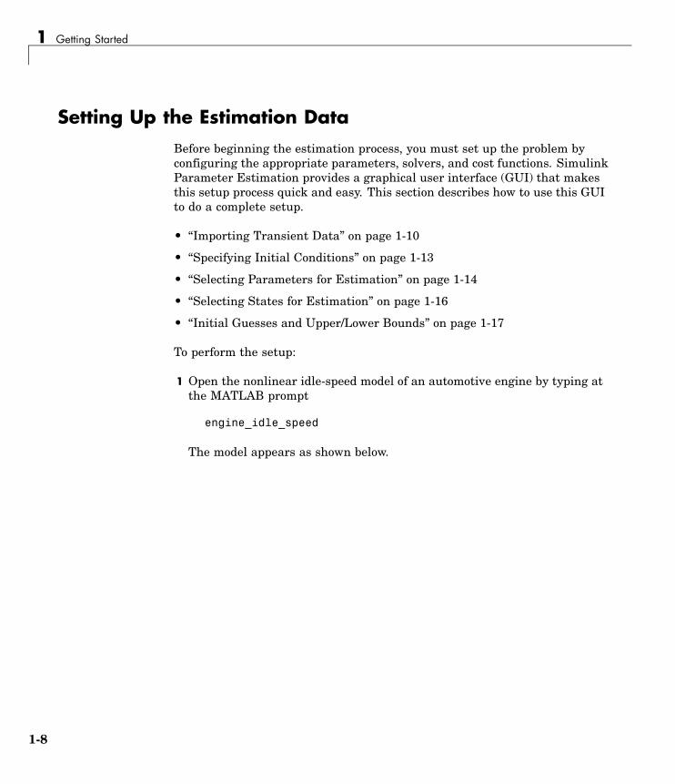
1 Open the nonlinear idle-speed model of an automotive engine by typing atthe MATLAB prompt
engine_idle_speed
The model appears as shown below.
1-8
Setting Up the Estimation Data
2 Open the Control and Estimation Tools Manager GUI by selecting Tools >Parameter Estimation in the Simulink model window.
The workspace directory tree displays the project name. Estimation tasksare organized inside the Estimation Task node.
1-9

1 Getting Started
Control and Estimation Tools Manager GUI
To add, delete, or rename the project or task:
1 Right-click the project or task node in the workspace directory tree.
2 Select the appropriate command from the shortcut menu.
When using the Control and Estimation Tools Manager for parameterestimation, you can
• Manage estimation projects.
• Select parameters and initial conditions to configure the estimation.
• Specify cost functions.
• Import experimental data (to be matched by the output of your Simulinkmodel).
• Specify the initial conditions of your model.
Importing Transient DataTo import transient (measured) data for your dynamic system:
1-10

Setting Up the Estimation Data
1 In the Control and Estimation Tools Manager, select Estimation Task >Transient Data in the workspace directory tree.
2 Right-click Transient Data and select New to create a new data set. Theidle-speed model of an automotive engine contains measured data storedin the iodata array.
3 Select the New Data node in the workspace directory tree.
Import Data into the Control and Estimation Tools Manager
To import the model input data:
1 Click the Input Data tab.
2 Right-click the first Data cell and select Import to open the Data Importdialog box.
1-11

1 Getting Started
3 Select iodata from the list of variables. The iodata array contains twocolumns: the first for model input data, and the second for model outputdata.
4 Enter 1 in the Assign columns field, and then click Import.
Note To import the time vector, select the Time/Ts cell in the Input Datatab and follow the same procedure — but select the time variable in theData Import dialog box instead.
To import the model output data:
1 Click the Output Data tab.
2 Right-click the first Data cell and select Import to open the Data Importdialog box.
3 Select iodata from the list of variables.
4 Enter 2 in the Assign columns field to use the second column of iodata,and then click Import.
1-12

Setting Up the Estimation Data
Note To import the time vector for output data, select the Time/Ts cell inthe Output Data tab and follow the same procedure — but select the timevariable in the Data Import dialog box instead. Enter 1 in the Assigncolumns field.
5 Click Close to close the Data Import dialog box.
Specifying Initial ConditionsBy default, the estimation uses initial conditions specified in the Simulinkmodel. If you want to specify initial conditions other than the defaults, usethe State Data pane. You can open it by selecting Transient Data > NewData in the workspace directory tree, and then clicking the State Data tab.
1-13

1 Getting Started
To specify an initial condition for a state:
1 Select the Data cell associated with the state.
2 Enter the initial conditions. In this example, enter -0.2 for State - 1 ofthe engine_idle_speed/Transfer Fcn. For State - 2, enter 0.
Selecting Parameters for EstimationTo select parameters for estimation:
1 In the Control and Estimation Tools Manager, select the Variables node inthe workspace directory tree to open the Estimated Parameters pane.
2 In the Estimated Parameters pane, click Add to open the SelectParameters dialog box.
1-14

Setting Up the Estimation Data
3 Select the last seven parameters: freq1, freq2, freq3, gain1, gain2,gain3, and mean_speed, and then click OK.
In general, you can enter parameters stored in one of the following by enteringinformation into the Specify expression field (separated by commas):
• Simulink parameter object
Example: For a Simulink parameter object k, type k.value.
• Structure
Example: For a structure S, type S.fieldname (where fieldname representsthe name of the field that contains the parameter).
• Cell array
Example: Type C{1} to select the first element of the C cell array.
• MATLAB array
Example: Type a(1:2) to select the first column of a 2-by-2 array called a.
1-15

1 Getting Started
Note You need not estimate the parameters selected here all at once. Youcan first select all the parameters that you are interested in, and then laterdecide which ones to estimate in a particular estimation.
Often, it is more practical to estimate a small group of parameters and use thefinal estimated values as a starting point for further estimation of parametersthat are trickier. Making these sorts of choices involves experience, intuition,and a solid understanding of the strengths and limitations of your Simulinkmodel.
Sometimes models have parameters that are not explicitly defined in themodel itself. For example, a gain k could be defined in the MATLABworkspace as k=a+b, where a and b are not defined in the model but k is used.To add these independent parameters to the Select Parameters dialog box, see“Estimating Independent Parameters” on page 1-49.
Selecting States for EstimationTo estimate initial conditions (or initial states) if they are not known:
1 In the Control and Estimation Tools Manager, select the Variables node inthe workspace directory tree.
2 Click the Estimated States tab.
3 Click Add. This opens the Select States dialog box.
1-16

Setting Up the Estimation Data
4 Examine the available states but do not select any for this example.
In general, you only choose to estimate those states that are not already inthe model.
Initial Guesses and Upper/Lower BoundsAfter you select parameters for estimation, the Control and Estimation ToolsManager looks like the following figure.
1-17

1 Getting Started
For each parameter, use the Default settings pane to specify the following:
• Initial guess — The value the estimation uses to start the process.
• Minimum — The smallest allowable parameter value. The default is -Inf.
• Maximum — The largest allowable parameter value. The default is +Inf.
• Typical value — The average order of magnitude. If you expect yourparameter to vary over several orders of magnitude, enter the numberthat specified the average order of magnitude you expect. For example, ifyour initial guess is 10, but you expect the parameter to vary between10 and 1000, enter 100 (the average of the order of magnitudes) for thetypical value.
1-18
Setting Up the Estimation Data
You use the typical value in two ways:
• To scale parameters with radically different orders of magnitude for equalemphasis during the estimation. For example, try to select the typicalvalues so that
anticipated valuetypical value
≅ 1
or
initial valuetypical value
≅ 1
• To put more of less emphasis on specific parameters. Use a larger typicalvalue to put more emphasis on a parameter during estimation.
1-19

1 Getting Started
Setting Up an Estimation ProjectAfter you import the transient data and select the parameters and any initialconditions (or states) to estimate, you are ready to configure the estimationsettings. To create a container that stores the estimation settings:
1 In the Control and Estimation Tools Manager, right-click Estimation inthe workspace directory tree and select New.
2 Click the New Estimation node.
• “Adding Data Sets” on page 1-20
• “Specifying and Setting Up Parameters” on page 1-22
• “Opening the Estimation Pane” on page 1-23
Adding Data SetsAfter you select the New Estimation node, the Data Sets tab appears.Here you choose the output data from the Simulink model that you want touse in the estimation.
In this example, select the check box to the right of the New Data data set.
1-20

Setting Up an Estimation Project
Note If you imported multiple data sets, you can select them for estimationby selecting the check box to the right of each desired data set. When usingseveral data sets, you increase the estimation precision. However, you alsoincrease the number of required simulations: for N parameters and M datasets, there are M*(2N+1) simulations per iteration.
Then, specify the weight of each output from this model by setting the Weightcolumn in the Output data weights table.
The relative weights are used to place more or less emphasis on specificoutput variables. The following are a few guidelines for specifying weights:
• Use less weight when an output is noisy.
• Use more weight when an output strongly affects parameters.
1-21

1 Getting Started
• Use more weight when it is more important to accurately match this modeloutput to the data.
Specifying and Setting Up ParametersSelect the New Estimation node in the workspace directory tree, and thenclick the Parameters tab in the Control and Estimation Tools Manager. Hereyou select which parameters to estimate and the range of values for theestimation.
Note When you set the estimation parameters here, such as Minimum andMaximum, this does not affect your settings in the Variables node. Youmake these choices on a per estimation basis. You can move data to and fromtheVariables node into the Estimation node.
1-22

Setting Up an Estimation Project
Here you select the parameters you want to estimate in the Estimate column.Enter initial values for your estimation parameters in the Initial Guesscolumn. The default values in the Minimum and Maximum columns are-Inf and +Inf, respectively, but you can select any range you want.
For this example, set gain1 to 10, gain2 to 100, gain3 to 50, and mean_speedto 500. Or, use any initial values you like.
If you have good reason to believe a parameter lies within a finite range, it isusually best not to use the default minimum and maximum values. Often,there is computational advantage in specifying finite bounds if you can. Itcan be very important to specify lower and upper bounds. For example, if aparameter specifies the weight of a part, be sure to specify 0 as the absolutelower bound if better knowledge is unavailable.
Opening the Estimation PaneClick the Estimation tab to specify a new estimation.
1-23

1 Getting Started
Before you start, you can click Estimation Options to specify variousalgorithm and simulation features. See “Selecting Optimization Methods”on page 1-42 for more information.
Display OptionsClicking Display Options opens this dialog box.
Clearing a check box means that data will not appear in the display tablefor the estimation.
1-24

Selecting Views for Plotting
Selecting Views for Plotting
Note An estimation must be created before creating views. Otherwise, theOptions table will be empty.
To watch the minimization progress:
1 Right-click the Views node in the Control and Estimation Tools Managerand select New.
2 In the workspace directory tree, select New View to open the View Setuppane.
3 Select the Cost function plot type by clicking the first cell in the PlotType column, located in the Select plot types table.
1-25

1 Getting Started
4 Select the Plot 1 check box in the Options table.
Click Show Plots. This displays an empty cost function plot. When yourun the estimation, the plot updates automatically.
Various types of plots are available, including
• Cost function — Plot the cost function values.
• Measured and simulated — Plot empirical data against simulated data.
• Parameter sensitivity — Plot the rate of change of the cost function as afunction of the change in the parameter. That is, plot the derivative of thecost function with respect to the parameter being varied.
• Parameter trajectory — Plot the parameter values as they change.
• Residuals — Plot the error between the experimental data and thesimulated output.
This figure shows the plot generated by running the estimation, as describedin “Running the Estimation” on page 1-28.
1-26

Selecting Views for Plotting
1-27

1 Getting Started
Running the EstimationIn the Control and Estimation Tools Manager, select the New Estimationnode and click the Estimation tab.
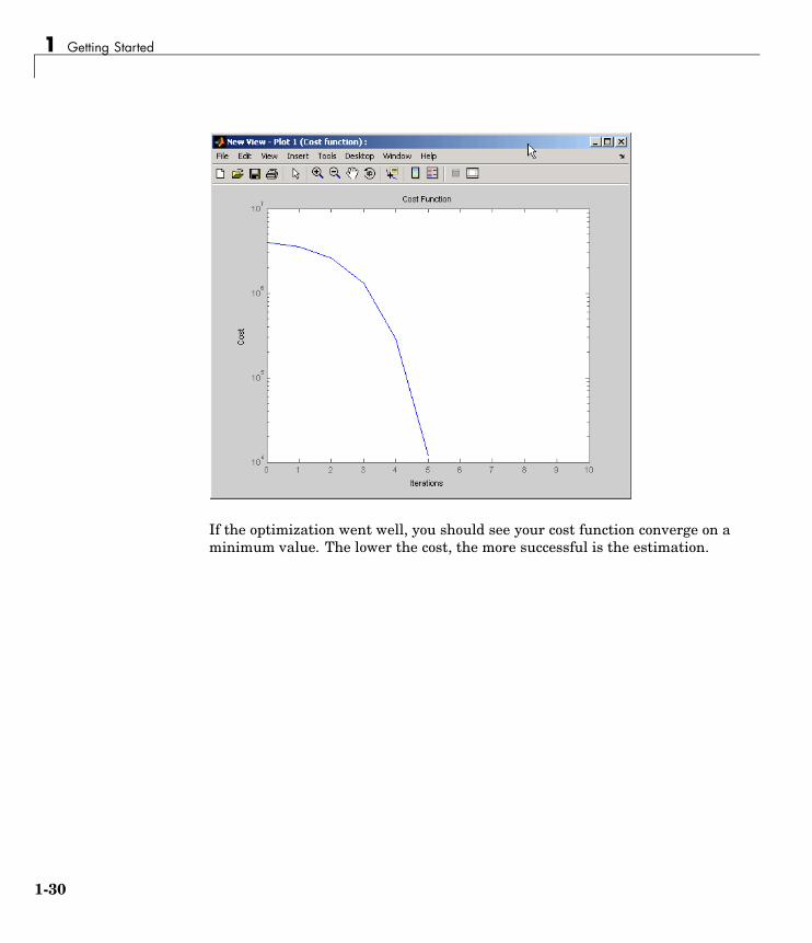
Click Start to begin the estimation process. At the end of the iterations, thewindow should resemble the following:
Usually, a lower cost function value indicates a successful estimation,meaning that the experimental data matches the model simulation with theestimated parameters.
The Estimation pane displays each iteration of the optimization algorithm.To see the final values for the parameters, click the Parameters tab.
1-28

Running the Estimation
The values of these parameters are also updated in the MATLAB workspace.So, if you specify the variable name in the Initial Guess column, you canrestart the estimation from where you left off at the end of a previousestimation.
The cost function minimization is plotted below.
1-29
1 Getting Started
If the optimization went well, you should see your cost function converge on aminimum value. The lower the cost, the more successful is the estimation.
1-30

Model Validation
Model ValidationAfter you complete an estimation, you can validate your results againstanother set of data.
• “Example: Validating the Engine Idle Speed Model” on page 1-32
• “Loading and Importing the Validation Data” on page 1-32
• “Performing Validation” on page 1-34
• “Residuals” on page 1-38
These are the basic steps needed to validate a model using the Control andEstimation Tools Manager:
1 Add the validation data to the Transient Data sets.
2 Add a new validation task under the Validation node in the workspacedirectory tree.
3 Edit the validation — select plot types you want from the ValidationSetup pane and select the validation data set you want to use.
4 Click Show Plots in the Validation Setup pane and view the results inthe plot window.
5 Compare the validation plots to the corresponding view plots to see ifthey match.
The basic difference between the validation and views features is that youcan run validations after your estimation is complete. All views should be setup before an estimation, and you can watch the views update in real time.Validations can use other validation data sets for comparison with the modelresponse. Also, validations appear after you have completed an estimationand do not update.
You can validate your data by comparing measured vs. simulated data foryour estimation data and validation data sets. Also, it is often useful tocompare residuals in the same way.
1-31

1 Getting Started
Example: Validating the Engine Idle Speed ModelIf you have not run the engine idle speed demo, type
engine_idle_speed
at the MATLAB prompt and run the estimation. If you haven’t run anestimation yet, see “How Simulink Parameter Estimation Works” on page 1-6.To save time, double-click the box in the upper-left corner of the model toimport data and populate the required fields in the Control and EstimationTools Manager.
engine_idle_speed Simulink Model
Now that the estimation data is loaded, and the estimation task has beencreated, the next step is to import validation data into the Control andEstimation Tools Manager.
Loading and Importing the Validation DataTo load the validation data, type
load iodataval
1-32

Model Validation
at the MATLAB prompt. This loads the data into the MATLAB workspace.The next step is to import this data into the tools manager. See “ImportingTransient Data” on page 1-10 for information on importing data, but thequickest way is to follow these steps:
1 Right-click the Transient Data node in the workspace directory tree inthe Control and Estimation Tools Manager and select New.
2 Select New Data 2 from the Transient data sets pane and click Edit.
3 Right-click the New Data (2) node in the workspace directory tree andselect Rename. Change the name of the data to Validation Data.(You can also change the name by double-clicking New Data (2) in theTransient data sets pane and clicking Rename.)
4 In the Input Data pane, select the Data cell associated with Channel- 1 and click Import. In the Data Import dialog box, select iodatavaland assign column 1 to the selected channel by entering 1 in the Assigncolumns field. Click Import to import the data.
5 Select the Time/Ts cell and import time using the Data Import dialog box.
6 Similarly, in the Output Data pane, select Time/Ts and import time.
1-33

1 Getting Started
7 In the Output Data pane, select the Data cell associated with Channel- 1 and click Import. Import the second column of data in iodataval byselecting it from the list in the Import Data dialog box and entering 2 in theAssign columns field. Click Import to import the data.
Your Control and Estimation Tools Manager should resemble this figure.
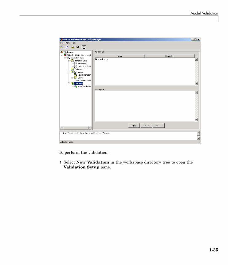
Performing ValidationAfter you import the data, right-click the Validation node and select New.This opens the Validations pane in the Control and Estimation ToolsManager.
1-34
Model Validation
To perform the validation:
1 Select New Validation in the workspace directory tree to open theValidation Setup pane.
1-35

1 Getting Started
2 Click the Plot Type cell for Plot 1 and select Measured and simulatedfrom the menu.
3 In the Options area, select Validation Data in the Validation data setlist. Click Show Plots to open a plot figure window as shown below.
1-36

Model Validation
Measured (Validation) Versus Simulated Data Plot
4 Compare this with the plot of measured and simulated data from theViews node of the workspace directory tree.
1-37
1 Getting Started
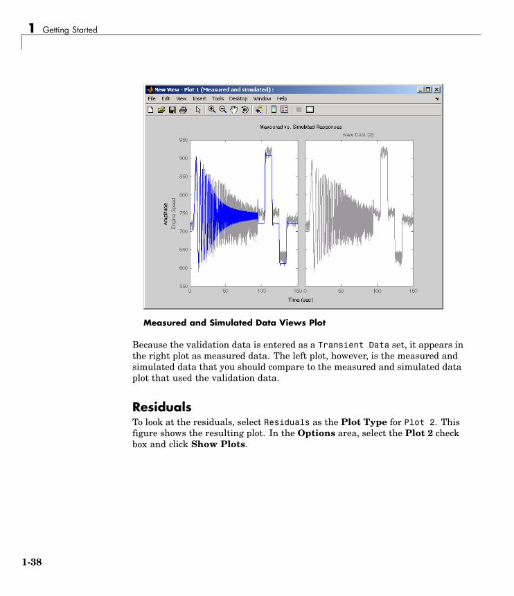
Measured and Simulated Data Views Plot
Because the validation data is entered as a Transient Data set, it appears inthe right plot as measured data. The left plot, however, is the measured andsimulated data that you should compare to the measured and simulated dataplot that used the validation data.
ResidualsTo look at the residuals, select Residuals as the Plot Type for Plot 2. Thisfigure shows the resulting plot. In the Options area, select the Plot 2 checkbox and click Show Plots.
1-38

Model Validation
Plot of Residuals Using the Validation Data
Compare the validation data residuals to the original data set residuals fromthe Views node in the workspace directory tree.
1-39

1 Getting Started
Plot of Residuals Using the Test Data
The plot on the left agrees with the plot of the residuals for the validationdata. The right side has no plot because residuals were not calculated for thevalidation data during the original estimation process.
1-40

Setting Options for Optimization
Setting Options for OptimizationYou can set several options to tune the results of the optimization. Theseoptions include the optimization algorithms and their tolerances.
• “Selecting Optimization Methods” on page 1-42
• “Selecting Optimization Termination Options” on page 1-43
• “Selecting Additional Optimization Options” on page 1-43
• “Specifying the Cost Function” on page 1-44
To set options for optimization:
1 Select the New Estimation node in the workspace directory tree.
2 Click the Estimation tab.
3 Click Estimation Options to open the Options dialog box.
1-41

1 Getting Started
4 Click the Optimization Options tab and specify the options, as describedin the following sections:
• “Selecting Optimization Methods” on page 1-42
• “Selecting Optimization Termination Options” on page 1-43
• “Selecting Additional Optimization Options” on page 1-43
• “Specifying the Cost Function” on page 1-44
Selecting Optimization MethodsBoth the algorithm and model size define the optimization method. Use theOptimization method area in the Options dialog box to set algorithm andthe model size.
For the Algorithm parameter, the four options are
• Gradient descent — Uses the Optimization Toolbox function fmincon tooptimize the response signal subject to the constraints
• Nonlinear least squares — Uses a nonlinear least squares optimizationalgorithm.
• Pattern search — Uses an advanced pattern search algorithm. Thisoption requires the Genetic Algorithm and Direct Search Toolbox.
• Simplex search — Uses the Optimization Toolbox function fminsearch,which is a direct search method to optimize the response. Simplex searchis most useful for simple problems and is sometimes faster than Functionminimization for models that contain discontinuities.
By default, the Model size parameter is set to Large scale. When thenumber of parameters you want to estimate is large, Model size must usethe default to increase computation speed. If your model is not very large, itmight be more efficient to select Medium scale. See the Optimization Toolboxdocumentation for more information about optimization methods.
1-42

Setting Options for Optimization
Selecting Optimization Termination OptionsSpecify termination options in the Optimization options area.
Several options define when the optimization terminates:
• Diff max change — The maximum allowable change in variables forfinite-difference derivatives. See fmincon in the Optimization Toolboxdocumentation for details.
• Diff min change — The minimum allowable change in variables forfinite-difference derivatives. See fmincon in the Optimization Toolboxdocumentation for details.
• Parameter tolerance — Optimization terminates when successiveparameter values change by less than this number.
• Maximum fun evals — The maximum number of cost functionevaluations allowed. The optimization terminates when the number offunction evaluations exceeds this value.
• Maximum iterations — The maximum number of iterations allowed. Theoptimization terminates when the number of iterations exceeds this value.
• Function tolerance — The optimization terminates when successivefunction values are less than this value.
By varying these parameters, you can force the optimization to continuesearching for a solution or to continue searching for a more accurate solution.
Selecting Additional Optimization OptionsAt the bottom of the Optimization options pane is a group of additionaloptimization options.
1-43
1 Getting Started
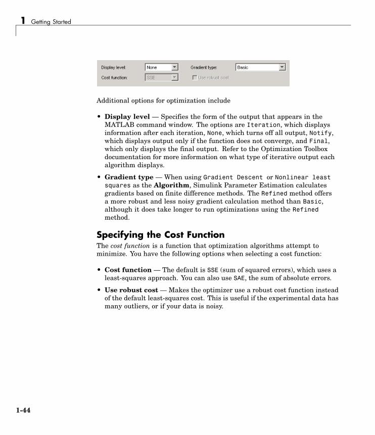
Additional options for optimization include
• Display level — Specifies the form of the output that appears in theMATLAB command window. The options are Iteration, which displaysinformation after each iteration, None, which turns off all output, Notify,which displays output only if the function does not converge, and Final,which only displays the final output. Refer to the Optimization Toolboxdocumentation for more information on what type of iterative output eachalgorithm displays.
• Gradient type — When using Gradient Descent or Nonlinear leastsquares as the Algorithm, Simulink Parameter Estimation calculatesgradients based on finite difference methods. The Refined method offersa more robust and less noisy gradient calculation method than Basic,although it does take longer to run optimizations using the Refinedmethod.
Specifying the Cost FunctionThe cost function is a function that optimization algorithms attempt tominimize. You have the following options when selecting a cost function:
• Cost function — The default is SSE (sum of squared errors), which uses aleast-squares approach. You can also use SAE, the sum of absolute errors.
• Use robust cost — Makes the optimizer use a robust cost function insteadof the default least-squares cost. This is useful if the experimental data hasmany outliers, or if your data is noisy.
1-44

Setting Options for the Simulation
Setting Options for the SimulationTo optimize the response signals of a model, Simulink Parameter Estimationruns simulations of the model.
• “Selecting Simulation Time” on page 1-46
• “Selecting Solvers” on page 1-46
To set options for simulation:
1 Select the New Estimation node in the workspace directory tree.
2 Click the Estimation tab.
3 Click Estimation Options to open the Options dialog box.
4 Click the Simulation Options tab and specify the options, as described inthe following sections.
1-45

1 Getting Started
Selecting Simulation Time
By default, Start time and Stop time are automatically computed based onthe start and stop times specified in the Simulink model. To set alternativestart and stop times for the optimization, enter them under Simulation time.
Selecting Solvers
When running the simulation, Simulink solves the dynamic system usingone of several solvers. You can specify several solver options using theSolver options area in the Options dialog box. The Type of solver can bevariable-step or fixed-step. Variable-step solvers keep the error withinspecified tolerances by adjusting the step-size the solver uses. Fixed-stepsolvers use a constant step-size. When your model’s states are likely to varyrapidly, a variable-step solver is often faster. See the Simulink documentationfor information about solvers.
Variable-Step SolversWhen you select Variable-step as the solver Type, you can choose any ofthe following as the Solver:
• discrete (no continuous states)
• ode45 (Dormand-Prince)
• ode23 (Bogacki-Shampine)
• ode113 (Adams)
1-46

Setting Options for the Simulation
• ode15s (stiff/NDF)
• ode23s (stiff/Mod. Rosenbrock)
• ode23t (Mod. stiff/Trapezoidal)
• ode23tb (stiff/TR-BDF2)
Variable-Step Solver OptionsWhen you select Variable-step as the solver Type, you can also set severalother parameters that affect the step-size of the simulation:
• Maximum step size — The largest step-size Simulink can use during asimulation.
• Minimum step size — The smallest step-size Simulink can use during asimulation.
• Initial step size — The step-size Simulink uses to begin the simulation.
• Relative tolerance — The largest allowable relative error at any step inthe simulation.
• Absolute tolerance — The largest allowable absolute error at any step inthe simulation.
• Zero crossing control — Set to on for the solver to compute exactlywhere the signal crosses the x-axis. This is useful when using functionsthat are nonsmooth and the output depends on when a signal crosses thex-axis, such as absolute values.
By default, Simulink automatically chooses values for these options. Tochoose your own values, enter them in the appropriate fields.
Fixed-Step SolversWhen you select Fixed-step as the solver Type, you can choose any of thefollowing as the Solver:
• discrete (no continuous states)
• ode5 (Dormand-Prince)
• ode4 (Runge-Kutta)
1-47

1 Getting Started
• ode3 (Bogacki-Shanpine)
• ode2 (Heun)
• ode1 (Euler)
When you select Fixed-step as the solver Type, you can also set Fixed stepsize, which determines the step-size the solver uses during the simulation.By default, Simulink automatically chooses a value for this option.
1-48

Estimating Independent Parameters
Estimating Independent ParametersSometimes parameters in your model depend on independent parameters thatdo not appear in the model. The following steps give an overview of how touse Simulink Parameter Estimation to estimate independent parameters:
1 Add the independent parameters to the model workspace (along withinitial values).
2 Define a Simulation Start function that runs before each simulation of themodel. This Simulation Start function defines the relationship between thedependent parameters in the model and the independent parameters inthe model workspace.
3 The independent parameters now appear in the Add Parameters dialogbox. Add these parameters to the list of parameters to be estimated.
Caution Avoid adding independent parameters together with theircorresponding dependent parameters to the lists of parameters to beestimated. Otherwise the estimation could give incorrect results. Forexample, when a parameter x depends on the parameters a and b, avoidadding all three parameters to the list.
Example: Estimating Independent ParamtersAssume that the parameter Kint in the model srotut1 is related to theparameters x and y according to the relationship Kint=x+y. Also assume thatthe initial values of x and y are 1 and -0.7 respectively. To estimate x and yinstead of Kint, first define these parameters in the model workspace. Todo this:
1 At the MATLAB prompt, type
srotut1
This opens the srotut1 model window.
2 Select View > Model Explorer from the srotut1 window to open theModel Explorer window.
1-49

1 Getting Started
3 In the Model Hierarchy tree, select the srotut1 > Model Workspacenode.
4 Select Add > MATLAB Variable to add a new variable to the modelworkspace. A new variable with a default name Var appears in theContents of: Model Workspace pane.
5 Double-click Var to make it editable and change the variable name to x.Edit the initial Value to 1.
6 Repeat steps 4 and 5 to add a variable y with an initial value of -0.7. TheModel Explorer window should resemble the following figure.
1-50

Estimating Independent Parameters
7 To add the Simulation Start function defining the relationship betweenKint and the independent parameters x and y, select File > ModelProperties in the srotut1 window.
8 In the Model Properties window, click the Callbacks tab.
9 Under Simulation start function, enter the name of a new M-file, forexample, srotut1_start.
10 Create a new M-file with this name. The contents of the M-file shoulddefine the relationship between the parameters in the model and theparameters in the workspace. For this example, the M-file should resemblethe following:
wks = get_param(gcs, 'ModelWorkspace')x = wks.evalin('x')y = wks.evalin('y')Kint = x+y;
Note You must first use the get_param function to get the variables x andy from the model workspace before you can use them to define Kint.
1-51

1 Getting Started
11 When you add a parameter to be estimated, x and y should now appearin the Add Parameters dialog box.
1-52

2
Estimating InitialConditions
Why Estimate Initial Conditions?(p. 2-2)
Reasons for estimating initialconditions of states in your model
Estimating Initial Conditionsfor Blocks with External InitialConditions (p. 2-3)
Tuning the initial conditions of ablock with external initial conditions
Example: Mass-Spring-DamperSystem (p. 2-4)
An example that takes youstep-by-step through an estimationof the initial position of a massattached to a spring

2 Estimating Initial Conditions
Why Estimate Initial Conditions?Often, sets of measured data are collected at various times and under differentinitial conditions. If you estimate parameters for your Simulink model usingone set, then try again with another, your parameter values may not match.Given that Simulink Parameter Estimation attempts to find constant valuesfor parameters, this is clearly a problem.
Fortunately, Simulink Parameter Estimation has features that make thistask simpler. The Control and Estimation Tools Manager has an EstimatedStates pane that lists the states available for initial condition estimation. So,you can estimate initial conditions using procedures that are similar to thoseyou use to estimate parameters. You can then use these initial conditionestimates as a basis for estimating parameters for your Simulink model.
This chapter focuses on the steps required to estimate initial conditions, andthen estimate the parameters from these initial conditions.
2-2

Estimating Initial Conditions for Blocks with External Initial Conditions
Estimating Initial Conditions for Blocks with ExternalInitial Conditions
When an integrator block uses an initial-condition port, which you specify byan IC block feeding into the integrator block, you cannot estimate the initialconditions (ICs) of the integrator using Simulink Parameter Estimation.This is because external ICs have priority over the ICs of a specific block tomaintain the integrity of the model.
To tune the ICs of an integrator block with external ICs, you must modify themodel to make the external signal into a tunable parameter. For example, youcan set the IC block that feeds into the integrator to be a tunable variablethat Simulink Parameter Estimation can estimate.
2-3

2 Estimating Initial Conditions
Example: Mass-Spring-Damper SystemThe figure below is a Simulink model of a mass-spring-damper system.
This example goes beyond what is included in the Simulink ParameterEstimation demo that uses this model by providing in-depth discussion ofeach task and discusses the following:
• “Model Parameters” on page 2-5
• “Setting Up the Estimation Project” on page 2-6
• “Importing Transient Data and Selecting Parameters for Estimation” onpage 2-7
• “Selecting Parameters and Initial Conditions for Estimation” on page 2-8
• “Creating the Estimation Task” on page 2-10
• “Running the Estimation and Viewing Results” on page 2-11
2-4

Example: Mass-Spring-Damper System
You can run the demo by seeing the listings under Simulink for SimulinkParameter Estimation on the Demo pane of the Help browser.
To open the model and two sets of model data with differing initial conditions,type
msd_system
at the MATLAB prompt.
Model ParametersThe Simulink msd_system model’s output is the displacement (or position)of the mass in a mass-spring-damper system, subject to a constant force F,and an initial condition, x0, for the mass displacement. x0 is indicated by theinitial condition of the Position integrator block. Click the Start Simulationbutton to run the simulation once and observe the response of the model totwo sets of parameter values.
2-5

2 Estimating Initial Conditions
The model parameters of interest are the mass, m, the viscous damping, b,and the spring constant, k. For more information about physical modelingof mass-spring-damper systems, see any elementary book on mathematicalmodeling or on automatic control systems.
For the estimation of the model parameters m, b, and k, this model uses twosets of experimental data. These data sets were obtained using two differentinitial positions, x0=0.1 and x0=0.3, and also contain additive noise. A plotof these data sets is shown in the figure above (top curves), along with thesimulated response (bottom curve) of the Simulink model msd_system forx0=-0.1 and a nominal set of parameter values, m=8, k=500, and b=100.
Setting Up the Estimation ProjectTo set up the estimation of initial conditions and then transient state spacedata, select Tools > Parameter Estimation in the msd_system modelwindow.
2-6

Example: Mass-Spring-Damper System
Importing Transient Data and Selecting Parametersfor EstimationThe process for importing transient data and selecting parameters forestimation is discussed in “Importing Transient Data” on page 1-10 and“Selecting Parameters for Estimation” on page 1-14.
1 In the Control and Estimation Tools Manager, select Estimation Task >Transient Data in the workspace directory tree.
2 Right-click Transient Data and select New to add a new data set.
3 Right-click the New Data node in the workspace directory tree and selectEdit to open the Input Data, Output Data, and State Data panes.
4 In the Output Data pane, click Import and add yexp1 to the Data columnand texp1 to the Time/Ts column of the msd_system/Position state.
5 If you like, right-click New Data in the workspace directory tree andrename it to Data set #1.
6 Repeat steps 1 to 5 to add a second data set, yexp2 and texp2, and renameit to Data set #2.
Your Control and Estimation Tools Manager should resemble this figure:
2-7

2 Estimating Initial Conditions
Selecting Parameters and Initial Conditions forEstimationFirst, select the parameters you want to estimate for the Simulink msd_systemmodel. In this case, select b, k, and m. To do this:
1 Select the Variables node in the workspace directory tree of the Controland Estimation Tools Manager.
2 Click the Estimation Parameters tab.
3 Click Add to open the Select Parameters dialog box.
4 Select the parameters b, k, and m, and then click OK.
2-8
Example: Mass-Spring-Damper System
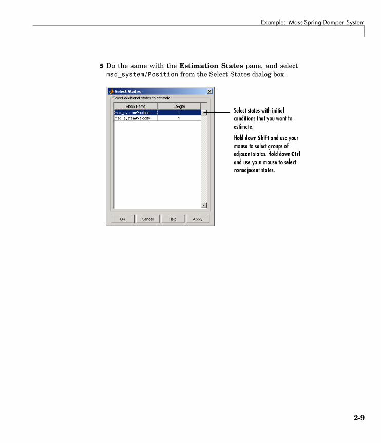
5 Do the same with the Estimation States pane, and selectmsd_system/Position from the Select States dialog box.
2-9

2 Estimating Initial Conditions
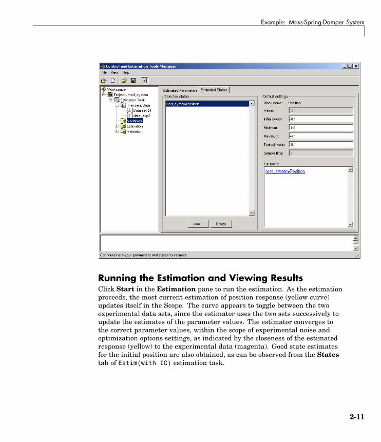
Your Control and Estimation Tools Manager should look like this.
Creating the Estimation TaskTo create the New Estimation task in the Control and Estimation ToolsManager, right-click the Estimation node in the workspace directory treeand select Add. While the initial velocity is also a state of the model, assume(for simplicity) that it is known to be 0. The estimation task for this caseis Estim (with IC).
In the Data Sets, Parameters, and States panes for the New Estimationtask, select all the check boxes in each table. Be sure to select Position forboth data sets in the States pane to estimate the initial condition for thespring’s position.
The initial position estimates for the two data sets are known to differ, but setthe initial state guesses for both data sets to -0.1.
2-10
Example: Mass-Spring-Damper System
Running the Estimation and Viewing ResultsClick Start in the Estimation pane to run the estimation. As the estimationproceeds, the most current estimation of position response (yellow curve)updates itself in the Scope. The curve appears to toggle between the twoexperimental data sets, since the estimator uses the two sets successively toupdate the estimates of the parameter values. The estimator converges tothe correct parameter values, within the scope of experimental noise andoptimization options settings, as indicated by the closeness of the estimatedresponse (yellow) to the experimental data (magenta). Good state estimatesfor the initial position are also obtained, as can be observed from the Statestab of Estim(with IC) estimation task.
2-11
2 Estimating Initial Conditions
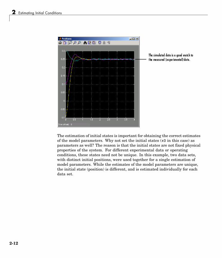
The estimation of initial states is important for obtaining the correct estimatesof the model parameters. Why not set the initial states (x0 in this case) asparameters as well? The reason is that the initial states are not fixed physicalproperties of the system. For different experimental data or operatingconditions, these states need not be unique. In this example, two data sets,with distinct initial positions, were used together for a single estimation ofmodel parameters. While the estimates of the model parameters are unique,the initial state (position) is different, and is estimated individually for eachdata set.
2-12

3
Preprocessing Data
Simulink Parameter Estimation provides for detrending, exclusion, andfiltering of data.
Why Preprocess Data? (p. 3-2) An introduction to datapreprocessing
Data Preprocessing Tool (p. 3-3) An introduction to a graphicaluser interface (GUI) for datapreprocessing
Excluding Data (p. 3-5) Various ways to exclude data fromyour data sets
Detrending and Filtering (p. 3-14) Various ways to detrend and filteryour data sets
Miscellaneous Data Handling(p. 3-16)
Additional features of the DataPreprocessing Tool

3 Preprocessing Data
Why Preprocess Data?When dealing with empirical data, it is often useful to remove outliers,smooth, detrend, or otherwise treat the data to make it more tractable foranalysis and estimation purposes. Simulink Parameter Estimation providesfeatures that perform the following tasks:
• Exclusion — Eliminate outliers, represent them as NaNs, or useinterpolation.
• Detrending — Remove mean values or a straight line trend.
• Filter — Smooth data using a first-order filter, an arbitrary transferfunction, or an ideal filter.
Data can overwrite existing data, or be stored in a new file.
3-2

Data Preprocessing Tool
Data Preprocessing ToolSimulink Parameter Estimation provides a GUI for data preprocessing, whichis the Data Preprocessing Tool. To open it:
1 Open the Control and Estimation Tools Manager.
2 Select the Transient Data node in the workspace directory tree, and thenchoose the data you want to modify in the Input Data, Output Data,or State Data pane.
3 Click Pre-process to open the Data Preprocessing Tool.
3-3
3 Preprocessing Data
In this chapter, the sample data is from the engine_idle_speed Simulinkmodel. See “How Simulink Parameter Estimation Works” on page 1-6 for anoverview of creating estimation projects and adding data sets.
With the Data Preprocessing Tool, you can
• Exclude data by selecting it with your mouse.
• Exclude data graphically by selecting regions on a plot.
• Exclude data by rules, such as upper or lower bounds.
• Detrend data.
• Filter data.
3-4

Excluding Data
Excluding DataThe three ways to exclude data are described in the following sections:
• “Selecting Data for Exclusion from the Data Editing Table” on page 3-5
• “Selecting Data for Exclusion from a Plot of the Data” on page 3-8
• “Selecting Data for Exclusion by a Rule” on page 3-11
You accomplish the first two manually, and for the last you specify a rule.When you exclude data using manual selection, the excluded data is shownas red. When you exclude data using a rule, the background color of the cellbecomes gray. When a portion of the data is excluded both manually and by arule, the data is red, and the background is gray.
Note Changes in data are visible everywhere. When you use the DataEditing table, you can view the results in the data plot.
Selecting Data for Exclusion from the Data EditingTableThe Data Editing table lists both the raw data set and the modified datathat you create.
3-5

3 Preprocessing Data
There are two tabs in the Data Editing pane: Raw data and Modifieddata. The Raw Data pane shows the working copy of the data. For example,if you exclude rows of data in the Raw data pane, the corresponding rowsof numbers become red in this table. By default the Modified data panerepresents the rows you removed by inserting NaNs.
3-6

Excluding Data
In the Modified data pane, you can choose to remove the excluded datacompletely or interpolate it. See “Miscellaneous Data Handling” on page3-16 for more information.
After you select data for exclusion, you can view it graphically by clickingExclude Graphically.
3-7

3 Preprocessing Data
As you make changes in the Data Editing pane, they immediately appear inthe Select Points for Preprocessing Rule window, and vice versa.
Selecting Data for Exclusion from a Plot of the DataYou can exclude data graphically. Click Exclude Graphically to open theSelect Points for Preprocessing Rule window.
3-8

Excluding Data
The way you exclude data is similar to the way you select a region forzooming: place your cursor in the Input Data plot and drag the mouse todraw a region of exclusion.
This figure shows an example of resulting data exclusion in the input data.
3-9

3 Preprocessing Data
In the Output Data plot, the excluded input data produces a blank area bydefault. This corresponds to the NaNs that now represent excluded data. Ifyou choose to interpolate or remove the excluded data, the output data showsthe interpolated points.
When you make changes in the Select Points for Preprocessing Rule window,they immediately appear in the Data Editing pane, and vice versa.
Selection PaneBy default, any box that you draw with your mouse selects data for exclusion,but you can toggle between exclusion and inclusion using the Selection paneon the left side of the Select Points for Preprocessing Rule window.
3-10

Excluding Data
Selecting Data for Exclusion by a RuleA more precise way to exclude data is to use mathematical rules. TheExclusion Rules pane in the Data Preprocessing Tool allows you to entercustomized rules for excluding data.
These are the rules you can use to exclude data:
• “Upper and Lower Bounds” on page 3-12
• “Outliers” on page 3-12
3-11

3 Preprocessing Data
• “MATLAB Expressions” on page 3-12
• “Flatlines” on page 3-12
Upper and Lower BoundsSelect the Bounds check box to activate upper and lower bound exclusion.Enter numbers in the Exclude X and Exclude Y fields for upper and lowerbound exclusion. By default, the exclusion rule is to include the boundaryvalues, but you can use the menu to exclude the boundaries as well.
OutliersSelect the Outliers check box to activate outlier exclusion. You can set theWindow length to any positive integer, and use confidence limits from 0 to100%. The window length specifies the number of data points used whencalculating outliers.
MATLAB ExpressionsUse the MATLAB expression field to enter any mathematical expressionusing MATLAB code. Use x as the variable name in your expression for thedata being tested.
FlatlinesIf you have areas of your data set where the data is constant, providing nonew information, then you can choose to exclude those data points as flatlines.The Window length field sets the minimum number of constant data pointsrequired to define the area as a flatline.
3-12

Excluding Data
Example of Rule ExclusionThis figure shows data with a region of the x-axis excluded.
3-13

3 Preprocessing Data
Detrending and FilteringYou can both detrend and filter data using the Detrend/Filtering pane inthe Data Preprocessing Tool.
• “Detrending” on page 3-14
• “Filtering” on page 3-14
DetrendingTo detrend, select the Detrending check box. You can choose constant orstraight line detrending. Constant detrending removes the mean of the datato create zero-mean data. Straight line detrending finds linear trends (in theleast-squares sense) and then removes them.
FilteringYou have these choices for filtering your data:
3-14

Detrending and Filtering
• First order — A filter of the type1
1τs +where τ is the time constant that you specify in the associated field.
• Transfer function — A filter of the type
a s a s a
b s b s bn
nn
n
mm
mm
+ + ++ + +
−−
−−
11
0
11
0
…
…
where you specify the coefficients as vectors in the associated Acoefficients and B coefficients fields.
• Ideal — An idealized (noncausal) filter, either stop or pass band. Specifyeither filter as a two-element vector in the Range (Hz) field. These filtersare ideal in the sense that there is no finite rolloff or ripple; the ends of theranges are perfectly horizontal in the frequency domain.
3-15

3 Preprocessing Data
Miscellaneous Data HandlingThere are a few miscellaneous data handling features in the DataPreprocessing Tool.
• “Handling Missing Data” on page 3-16
• “Loading Data and Saving Modified Data Sets” on page 3-16
Handling Missing DataYou can use the Missing Data Handling pane at the bottom of the DataPreprocessing Tool to remove rows of data, or to interpolate between pointsto fill in missing data.
Removing RowsIf you select the Remove rows where check box, the affected rows areremoved from the Modified data pane. If you have multiple columns ofdata, select all to remove rows in which all the data is excluded. Select anyto remove any excluded cell. In the case of one-column data, any and allare equivalent.
InterpolationYou have two choices if you want to interpolate data: zero-order hold (zoh)and linear interpolation (Linear). Select the Interpolate missing valuesusing interpolation method check box and choose which method you wantfrom the list. The results appear in the Modified data pane.
Loading Data and Saving Modified Data SetsAt the top of the Data Preprocessing Tool, there is a region for selecting datasets for preprocessing, and for saving modified data sets.
3-16

Miscellaneous Data Handling
When you have multiple data sets, select the one you want to preprocess fromthe Modify data from list.
To overwrite an existing data set, select the existing dataset option andchoose the data set you want to overwrite. If you want to save the dataset under a new name, select new dataset and type the new name in theassociated field.
3-17

3 Preprocessing Data
3-18

4
Managing Multiple Projects
Simulink Parameter Estimation works seamlessly with other MathWorksproducts to perform multiple tasks on multiple projects.
Multiple Projects and Tasks (p. 4-2) A brief discussion of handlingmultiple projects with multiple tasks
Saving Control and Estimation ToolsManager Projects (p. 4-3)
How to save projects for later
Opening Control and EstimationTools Manager Projects (p. 4-4)
How to open existing projects

4 Managing Multiple Projects
Multiple Projects and TasksThe Control and Estimation Tools Manager works seamlessly with productsin the Controls and Estimation family. In particular, if you have licensesfor Simulink Control Design or Model Predictive Control, you can use theseproducts to perform tasks on projects that you have created in SimulinkParameter Estimation, and vice versa.
This figure shows a tools manager with multiple projects and multiple tasks.
You can save projects individually, or group multiple projects together in onesaved file. This chapter describes how to do this.
4-2

Saving Control and Estimation Tools Manager Projects
Saving Control and Estimation Tools Manager ProjectsA Control and Estimation Tools Manager project can consist of multipletasks including those from Simulink Control Design, Simulink ParameterEstimation, and the Model Predictive Control Toolbox. Each task containsdata, objects, and results for the analysis of a particular model.
To save your project as a MAT-file, select File > Save in the Control andEstimation Tools Manager window.
To save multiple projects within one file:
1 In the Save Projects dialog box, select the projects that you want to save.
2 Click OK.
3 Choose a directory and name for your project file by either browsing for afile or typing the full path and filename in the Save as field. Click Save.
4-3

4 Managing Multiple Projects
Opening Control and Estimation Tools Manager ProjectsTo open previously saved projects, select File > Load in the Control andEstimation Tools Manager window.
In the Load Projects dialog box, choose a project file by either browsing forthe directory and file, or by typing the full path and filename in the Loadfrom field. Project files are always MAT-files. The projects within this fileappear in the Projects list.
Select the projects that you want to load, then click OK. When a file containsmultiple projects, you can choose to load them all or just a few.
4-4

5
Adaptive Lookup Tables
What Are Lookup Tables? (p. 5-2) A brief description of the lookuptable concept
How Adaptive Lookup Tables Work(p. 5-3)
More details on adaptive lookuptables
Implementation of Adaptive LookupTables (p. 5-4)
What adaptive lookup tables looklike in Simulink
Example: n-D Adaptive LookupTable (p. 5-8)
An example using amultidimensional adaptive lookuptable

5 Adaptive Lookup Tables
What Are Lookup Tables?Lookup tables are used to store numeric data in a multidimensional arrayformat. In the simpler two-dimensional case, lookup tables can be representedby matrices. Each element of a matrix is a numerical quantity, which can beprecisely located in terms of two indexing variables. At higher dimensions,lookup tables can be represented by multidimensional matrices, whoseelements are described in terms of a corresponding number of indexingvariables.
Lookup tables provide a means to capture the dynamic behavior of a physical(mechanical, electronic, software) system. The behavior of a system withM inputs and N outputs can be approximately described by using N lookuptables, each consisting of an array with M dimensions.
Lookup tables are usually generated by experimentally collecting orartificially creating the input and output data of a system. In general, asmany indexing parameters are required as the number of input variables.Each indexing parameter may take a value within a predetermined set ofdata points, which are called the breakpoints. The set of all breakpointscorresponding to an indexing variable is called a grid. So, a system withM inputs is girded by M sets of breakpoints. Given the input data, thebreakpoints are then used to locate the array elements, where the output dataof the system are stored. For a system with N outputs, N array elements arelocated and the corresponding data are stored at these locations.
Once a lookup table is created using the input and output measurements asdescribed above, the corresponding multidimensional array of values can beused in applications without the need of remeasuring the system outputs. Infact, only the input data is required to locate the appropriate array elementsin the lookup table and the approximate system output can be read from thedata stored at these locations. Therefore, a lookup table provides a suitablemeans of capturing the input-output mapping of a static system in the form ofnumeric data stored at predetermined array locations.
5-2

How Adaptive Lookup Tables Work
How Adaptive Lookup Tables WorkThe generation of lookup tables as described above establishes a permanentand static mapping of input-output behavior of a physical system. Staticallydefined lookup tables cannot accommodate the time-varying behavior(characteristics) of a physical plant. On the other hand, it is well knownthat the behavior of actual physical systems often vary with time due towear, environmental conditions, and manufacturing tolerances. Under suchvariations, the static mapping of input-output behavior of a plant describedby the lookup table may no longer provide a valid representation of the plantcharacteristics.
Adaptive lookup tables, on the other hand, incorporate the time-varyingbehavior of physical plants into the lookup table generation and maintenanceprocess while providing all of the functionality of a regular lookup table.
The adaptive lookup table receives the input and output measurements of aplant’s behavior, which are then used to dynamically create and update thecontent of the underlying lookup table. In addition to requiring the input datato create the lookup table, the adaptive lookup table also uses the outputdata of the plant to recalculate the table values. As an example, the outputdata of the plant can be collected by placing sensors at appropriate locationsin a physical system.
The input measurements are used to locate the array elements by comparingthese input values with the breakpoints defined for each indexing variable.Next, the output measurements are used to recalculate the numeric valuestored at these array locations. However, unlike a regular table, which onlystores the array data before the actual use of the lookup table, the adaptivetable continuously improves the content of the lookup table. This continuousimprovement of the table data is referred to as the adaptation or learningprocess.
The adaptation process involves statistical and signal processing algorithmsto recapture the input-output behavior of the plant. The adaptive lookuptable always tries to provide a valid representation of the plant dynamicseven though the plant behavior may be time varying. The underlying signalprocessing algorithms are also robust against reasonable measurement noiseand they provide appropriate filtering of noisy output measurements.
5-3

5 Adaptive Lookup Tables
Implementation of Adaptive Lookup TablesThis section discusses the following topics related to Adaptive Lookup Tables:
• “Adaptive Lookup Table Library” on page 5-5
• “Using Adaptive Lookup Tables in Simulink Models” on page 5-5
• “Real-Time Lookup Tables” on page 5-6
• “Setting Adaptive Lookup Table Parameters” on page 5-7
The MathWorks implements Adaptive Lookup Tables as Simulink blocks.These blocks create multidimensional lookup tables from measured orsimulated data. The inputs and outputs of a n-D Adaptive Lookup Tableblock with two inputs are shown below.
Adaptive Lookup Table Block Showing Inputs and Outputs
The following are descriptions of the input and output parameters:
• The inputs u and y are the coordinate data and system outputmeasurements, respectively. For example, if you want to create a lookuptable to model the behavior of an engine’s efficiency as a function of enginerpm and manifold pressure, u = [rpm, pressure] and y = [efficiency].
• The initial table data may be entered either as a dialog box parameter(by double-clicking the block) or as an input port (i.e., the input port Tinin the figure). You can start, stop, and reset the adaptation through theEnable input port.
5-4

Implementation of Adaptive Lookup Tables
• The outputs of the block include the value of the currently adapted tablecell (Y), the number (N) of that cell (which may be specified through theblock dialog box), and if required, the whole adapted table data (Tout).
Adaptive Lookup Table LibraryThree adaptive lookup tables are available in Simulink Parameter Estimation.
The three blocks are
• Adaptive Lookup Table (1D Stair-Fit) — One-dimensional adaptive lookup
• Adaptive Lookup Table (2D Stair-Fit) — Two-dimensional adaptive lookup
• Adaptive Lookup Table (nD Stair-Fit) — Multidimensional adaptive lookup(use this for dimension 3 or higher)
Using Adaptive Lookup Tables in Simulink ModelsA typical Simulink diagram using an adaptive lookup table block is shownbelow.
5-5

5 Adaptive Lookup Tables
Simulink Diagram Using an Adaptive Lookup Table
In this figure, the Experiment Data block imports a set of experimental datainto the Simulink environment through MATLAB workspace variables. Theinitial table is specified through a constant matrix block. When the simulationruns, the initial table begins to adapt to new data inputs and the resultingtable is copied to the block’s output.
Real-Time Lookup TablesYou can use experimental data from sensor measurements collected byrunning various tests on a system in real time. The measured data is thensent to the adaptive table block to generate a lookup table describing therelation between the system inputs and output.
The Adaptive Lookup Table block may also be used in a real-time environment,where some time-varying properties of a system need to be captured. Thiscan be done by generating C code using Real-Time Workshop®, which canthen be run in an xPC or dSpace environment. Since the adaptation may bestarted, stopped, or reset if desired, some logic may be used to adapt the tabledata only when it is desired. The Cell No output, and the Enable and Lockinputs facilitate this process. The Enable input is used to start and stop the
5-6

Implementation of Adaptive Lookup Tables
adaptation, while the Lock input is used to update only one of the table cells.The Lock input combined with some logic using the Cell No output providethe means for updating only the desired table cells during a simulation run.
Setting Adaptive Lookup Table ParametersAdaptive lookup tables are highly configurable, as shown below.
n-D Adaptive Lookup Table dialog box
For details on how to set these parameters, see the individual reference pages.
5-7

5 Adaptive Lookup Tables
Example: n-D Adaptive Lookup TableThis example shows an n-D adaptive lookup table at work and includes manyof the key features associated with adaptive lookup tables. Type
enginetable
at the MATLAB prompt to open this model.
This model has several key features:
• Input — The adaptive lookup table input is the experimental data. It isalso possible to make the original table itself an input.
• An enable feature — You can turn the adaptation on and off during theestimation to see how the basic features work.
• A lock feature — You can lock the table so that only one cell is adapting.This is useful if you have one section in your data that is highly erratic orotherwise difficult for the algorithm to handle.
5-8

Example: n-D Adaptive Lookup Table
• Output — Adaptive lookup breakpoints are the output data.
Running the ExampleTo start the enginetable simulation, select Simulation > Start. Or, onMicrosoft Windows, click the Start Simulation button in the Simulinktoolbar.
The simulation begins by populating the adaptive lookup table with randomdata. This figure shows the input and adaptive data side by side.
As the simulation progresses, the surface on the right adapts to match themeasured input data. This figure shows the final adaptation.
5-9

5 Adaptive Lookup Tables
The fit is quite good. Try using the enable and lock features to see how theychange the adaptation.
5-10

6
Estimating from theCommand Line
Simulink Parameter Estimation provides an object-oriented command-lineAPI for the estimation problem.
Introduction (p. 6-3) A brief discussion of the estimationproblem in an object-oriented context
Example: Estimating Parametersand Initial Conditions of the F14Model (p. 6-5)
How to create and simulatean estimation project from thecommand line
Creating and CustomizingEstimation Projects (p. 6-14)
Using properties and methods tospecify features of the estimationproject
Creating Transient Data Objects(p. 6-15)
How to instantiate and use transientdata objects, which contain inputand output data
Creating State Data Objects (p. 6-20) How to instantiate and use state dataobjects, which contain informationabout known states in your Simulinkmodel
Creating Transient ExperimentObjects (p. 6-23)
How to instantiate and useparameter objects, which maintaindata about parameters you want toestimate
Creating Parameter Objects (p. 6-26) How to instantiate and use stateobjects, which maintain data aboutthe block states you want to estimate

6 Estimating from the Command Line
Creating State Objects (p. 6-30) How to instantiate and use transientexperiment objects
Creating Estimation Objects (p. 6-34) How to instantiate and useestimation objects, which coordinateyour model, experiment, parameter,and state objects
6-2

Introduction
IntroductionIn addition to the Control and Estimation Tools Manager, Simulink ParameterEstimation provides a collection of functions for performing parameterand state estimation. These functions perform the same tasks as the toolsmanager, but have the advantages of command-line execution. Whenyou perform a state or parameter estimation using Simulink ParameterEstimation GUI, Simulink Parameter Estimation creates MATLAB objectsfor all the states and parameters of your model. If you have a large numberof states or parameters, this can use up large amounts of memory and causecomputational delays. With the command-line approach, only those statesand parameters that you select are assigned MATLAB objects, which is moreefficient.
In addition, the command-line approach is useful for batch jobs, where, forexample, you may want to test large numbers of models.
Note Simulink Parameter Estimation uses MATLAB objects to performestimation tasks. This chapter discusses what you need to know aboutobject-oriented programming for using Simulink Parameter Estimation,but see the MATLAB Programming documentation for a description ofobject-oriented programming in MATLAB.
The command-line interface for Simulink Parameter Estimation requires aSimulink model as a starting point for analysis and estimation. Once you haveselected a candidate model, the estimation process consists of these steps:
1 Defining experiments consisting of empirical data sets and the operatingconditions and/or initial conditions of your model
2 Selecting the variables and states to be estimated
3 Performing the estimation
4 Reviewing the results and iterating as necessary
5 Validating estimation results
6-3

6 Estimating from the Command Line
The following sections discuss these topics:
• “Example: Estimating Parameters and Initial Conditions of the F14 Model”on page 6-5 — How to perform the estimation process using command-linefunctions
• “Creating and Customizing Estimation Projects” on page 6-14 — How touse methods and properties to customize your estimation project’s features
6-4

Example: Estimating Parameters and Initial Conditions of the F14 Model
Example: Estimating Parameters and Initial Conditionsof the F14 Model
To define an experiment, you must start with a Simulink model. For thisexample, type
f14
to load the F14 fighter jet model into the MATLAB workspace. The figurebelow shows the f14 model.
F14 Fighter Jet Model
This example outlines the basics of constructing an estimation project usingobject-oriented code. Only what you need to run the example is presented inthis section.
• “Baseline Simulation” on page 6-6
6-5

6 Estimating from the Command Line
• “Creating a Transient Experiment Object” on page 6-7
• “Assigning Experimental Data to Inputs and Outputs of the Model” onpage 6-8
• “Creating Parameter Objects for Estimation” on page 6-9
• “Creating an Estimation Object and Running the Estimation” on page 6-10
See “Creating and Customizing Estimation Projects” on page 6-14 for detailson all the properties and methods associated with parameter estimation.
Baseline SimulationBefore running an estimation, you need a baseline for data comparison. First,you must choose parameters and states’ initial conditions for estimation. Thisexample uses Ta, the actuator time constant, and Zd and Md, the verticalvelocity and pitch rate gains, respectively. Then use the code below to run theSimulink f14 model. Note that this is standard Simulink code and does notinvolve Simulink Parameter Estimation in any way. See sim in the SimulinkReference documentation for information about running Simulink modelsfrom the MATLAB command line.
%% Open the model and load experimental data.open_system('f14')load f14_estim % Load empirical I/O data.
%% Set initialize unknown parameters% Actuator time constant (ideal: Ta = 0.05)Ta = 0.5;
% Aircraft dynamic model parameters (ideal: Md = -6.8847,% Zd = -63.998)Md = -1; Zd = -80;
%% Plot measured data and simulation results[T,X,Y] = sim('f14', time, [], [time iodata(:,1)]);plot(time, iodata(:,2:3), T, Y, ' ');legend( 'Measured angle of attack', 'Measured pilot g force', ...
'Simulated angle of attack', 'Simulated pilot g force');
The following figure appears.
6-6

Example: Estimating Parameters and Initial Conditions of the F14 Model
As you can see, the measured and simulated data are a poor match. Therest of this section describes how to estimate values for Ta, Zd, and Md thatresult in a better match of data sets.
Creating a Transient Experiment ObjectAfter you have a model and identify the parameters you want toestimate, the next step is to create the objects required for an estimation.ParameterEstimator is both the name of the class and the object instantiatedby that class. Classes are created by a constructor; objects are created byinvoking the class name with parameters.
First, create an estimation project object. This is the constructor syntax:
hExp = ParameterEstimator.TransientExperiment('f14');
MATLAB responds with information about the f14 model.
6-7

6 Estimating from the Command Line
Experimental transient data set for the model 'f14':
Output Data(1) f14/alpha (rad)(2) f14/Nz Pilot (g)
Input Data(1) f14/u
Initial States(1) f14/Actuator Model(2) f14/Aircraft Dynamics Model/Transfer Fcn.1(3) f14/Aircraft Dynamics Model/Transfer Fcn.2(4) f14/Controller/Alpha-sensor Low-pass Filter(5) f14/Controller/Pitch Rate Lead Filter(6) f14/Controller/Proportional plus integral compensator(7) f14/Controller/Stick Prefilter(8) f14/Dryden Wind Gust Models/Q-gust model(9) f14/Dryden Wind Gust Models/W-gust model
Assigning Experimental Data to Inputs and Outputsof the ModelAfter you create a ParameterEstimator object, assign input and outputexperimental (i.e., empirical) data.
%% Create objects to represent the experimental data sets.set(hExp.InputData(1), 'Data', iodata(:,1), 'Time', time);
set(hExp.OutputData(1), 'Data', iodata(:,2), 'Time', ...time, 'Weight', 5);
set(hExp.OutputData(2), 'Data', iodata(:,3), 'Time', time);
Note In general, for models with multiple inputs and outputs, you mustindependently assign one data object to each input and output port. Thedata object you assign to a specific port can be a vector or a matrix thatcorresponds to that channel. You cannot use a single I/O port to representmultiple channels.
6-8

Example: Estimating Parameters and Initial Conditions of the F14 Model
Creating Parameter Objects for EstimationTo activate parameters for estimation, you must create parameter objects forthe parameters you want to estimate. For this example, use Ta, the actuatortime constant, and Zd and Md, the vertical velocity and pitch rate gains,respectively. The Zd and Md gains are located in the F14 aircraft dynamicssubsystem.
First, create ParameterEstimator objects for the parameters you want toestimate.
%% Create objects to represent parameters.hPar(1) = ParameterEstimator.Parameter('Ta');set(hPar(1), 'Minimum', 0.01, 'Maximum', 1, 'Estimated', true)
hPar(2) = ParameterEstimator.Parameter('Md');set(hPar(2), 'Minimum', -10, 'Maximum', 0, 'Estimated', true)
hPar(3) = ParameterEstimator.Parameter('Zd');set(hPar(3), 'Minimum', -100, 'Maximum', 0, 'Estimated', true)
6-9

6 Estimating from the Command Line
%% Create objects to represent initial states.hIc(1) = ParameterEstimator.State('f14/Actuator Model');set(hIc(1), 'Minimum', 0, 'Estimated', false);
You can also use dot notation here. For example, instead of
set(hPar(2), 'Minimum', -10, 'Maximum', 0, 'Estimated', true)
you can write
hPar(2).Estimated=true;hPar(2).Minimum=-10;hPar(2).Maximum=0;
Creating an Estimation Object and Running theEstimationFinally, create an estimation object and run the estimation, using gcs to getthe full pathname to the Simulink model.
hEst = ParameterEstimator.Estimation(gcs, hPar, hExp);hEst.States = hIc;
%% Setup estimation optionshEst.OptimOptions.Algorithm = 'lsqnonlin';hEst.OptimOptions.GradientType = 'refined';hEst.OptimOptions.Display = 'iter';
%% Run the estimationestimate(hEst);
%% Plot measured data and final simulation results[T,X,Y] = sim('f14', time, [], [time iodata(:,1)]);figureplot(time, iodata(:,2:3), T, Y, ' ');legend( 'Measured angle of attack', 'Measured pilot g force', ...
'Simulated angle of attack', 'Simulated pilot g force');
6-10
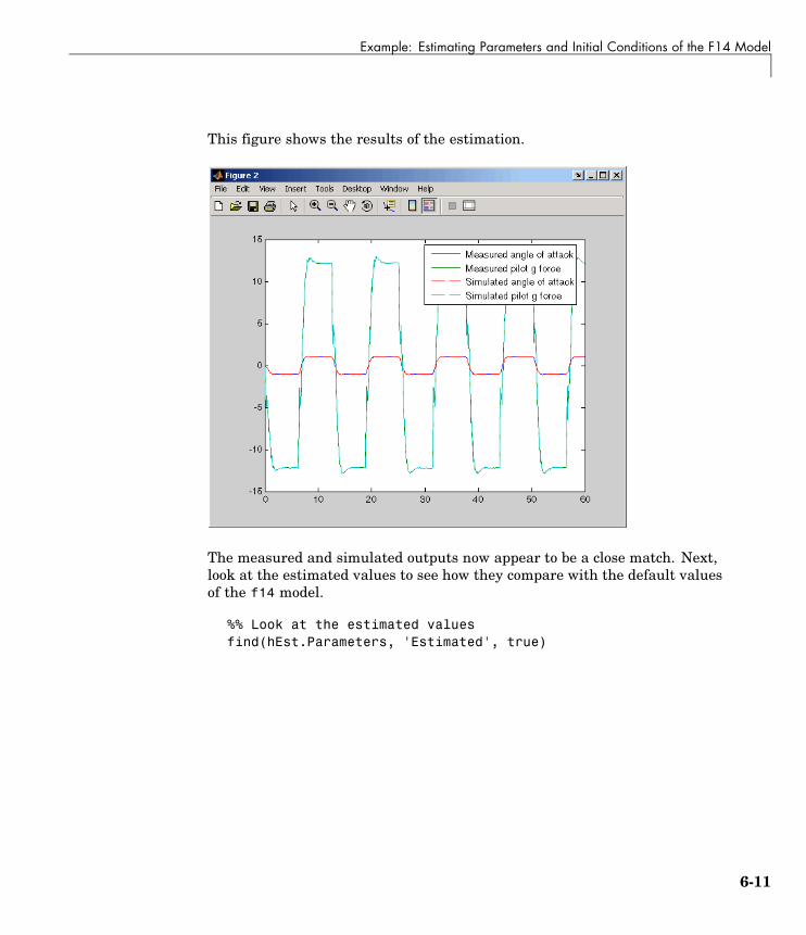
Example: Estimating Parameters and Initial Conditions of the F14 Model
This figure shows the results of the estimation.
The measured and simulated outputs now appear to be a close match. Next,look at the estimated values to see how they compare with the default valuesof the f14 model.
%% Look at the estimated valuesfind(hEst.Parameters, 'Estimated', true)
6-11

6 Estimating from the Command Line
MATLAB responds with
(1) Parameter data for 'Ta':
Parameter value : 0.05Initial guess : 0.5
Estimated : true
Referenced by:
(2) Parameter data for 'Md':
Parameter value : -6.884Initial guess : -1
Estimated : true
Referenced by:
(3) Parameter data for 'Zd':
Parameter value : -63.99Initial guess : -80
Estimated : true
Referenced by:
6-12

Example: Estimating Parameters and Initial Conditions of the F14 Model
Note You can use the find command to identify scalar, vector, or matrixparameters. The dimensions of the Estimated value you specify as the findargument must match the dimensions of the parameters you are trying tofind. For example,
find(hEst.Parameters, 'Estimated', true)
finds only scalar estimated parameters. However,
find(hEst.Parameters, 'Estimated', [true;true])
finds only vector estimated parameters with dimensions 1-by-2 and excludesall scalar parameters.
You can verify that these values match the default values of the f14 model byclearing your workspace, loading the model, and checking the values.
clear allf14whos
6-13
6 Estimating from the Command Line
Creating and Customizing Estimation ProjectsThe following sections describe in more detail how to create and modifytransient data and estimation objects:
• “Creating Transient Data Objects” on page 6-15
• “Creating State Data Objects” on page 6-20
• “Creating Transient Experiment Objects” on page 6-23
• “Creating Parameter Objects” on page 6-26
• “Creating State Objects” on page 6-30
• “Creating Estimation Objects” on page 6-34
First, a quick look at terminology:
• Objects are instantiations of classes.
• Classes contain, or rather, define, properties and methods.
• You use a constructor to create an instance of an object, and use the setmethod or dot notation to modify the properties of your objects.
6-14

Creating Transient Data Objects
Creating Transient Data ObjectsEstimating parameters requires a transient data object, which you createusing a constructor. The syntax to create a transient data object is
% I/O port blockh = ParameterEstimator.TransientData('block');% Internal blockh = ParameterEstimator.TransientData('block',portnumber);
h = ParameterEstimator.TransientData('block',data,time);h = ParameterEstimator.TransientData('block',data,Ts);h = ParameterEstimator.TransientData('block',portnumber,data,time);h = ParameterEstimator.TransientData('block',portnumber,data,Ts);
• “Properties of Transient Data Objects” on page 6-15
• “Modifying Properties of Transient Data Objects” on page 6-18
• “Using Class Methods” on page 6-19
Properties of Transient Data ObjectsDescriptions of properties of the transient data object and the associatedinput parameters are given below.
Transient Data Object Properties
Property Description
Block Name of the Simulink block with which the data isassociated. Must be a string.
PortType The type of signal that this object represents is determinedin the constructor from the Block property, which may beInport, Outport, or Signal.
PortNumber For data associated with the outputs of regular blocksor subsystems, this property specifies the output portnumber of interest. The default value is 1.
6-15

6 Estimating from the Command Line
Transient Data Object Properties (Continued)
Property Description
Dimensions Dimensions of the data required for this data set. It iscomputed from the CompiledPortDimensions property ofthe appropriate port of the block, and it defines the sizeof other properties. Currently, Simulink supports scalar,vector, or matrix signals, so Dimensions is either a scalaror a 1-by-2 array.
Data Actual experimental data. Its size must be consistentwith the Dimensions property. To conform with Simulinkconventions, the data is stored in the following formats:
• Scalar or vector-valued data. The data is of the form Nsm, where Ns is the number of data samples, and m isthe number of channels in the signal.
• Multidimensional data (matrix and higher dimensions).The data is of the form m1 . . . mn Ns, where Ns isthe number of data samples, and mi is the number ofchannels in the ith dimension of the signal.
• For missing or unspecified data, NaNs are used.
Ts,Tstart,Tstop
For uniformly sampled data, Ts is the sample time andTstart is the start time of the signal. The stop time Tstopand the time vector Time are given by
Tstop = Tstart + Ts * (Ns -1)
Time = Tstart : Ts : Tstop
For nonuniform time data, Ts is set to NaN, and the startand stop times are calculated from the time vector.
6-16
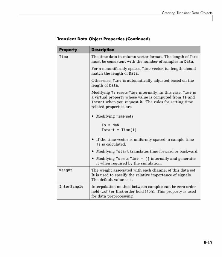
Creating Transient Data Objects
Transient Data Object Properties (Continued)
Property Description
Time The time data in column vector format. The length of Timemust be consistent with the number of samples in Data.
For a nonuniformly spaced Time vector, its length shouldmatch the length of Data.
Otherwise, Time is automatically adjusted based on thelength of Data.
Modifying Ts resets Time internally. In this case, Time isa virtual property whose value is computed from Ts andTstart when you request it. The rules for setting timerelated properties are
• Modifying Time sets
Ts = NaNTstart = Time(1)
• If the time vector is uniformly spaced, a sample timeTs is calculated.
• Modifying Tstart translates time forward or backward.
• Modifying Ts sets Time = [] internally and generatesit when required by the simulation.
Weight The weight associated with each channel of this data set.It is used to specify the relative importance of signals.The default value is 1.
InterSample Interpolation method between samples can be zero-orderhold (zoh) or first-order hold (foh). This property is usedfor data preprocessing.
6-17

6 Estimating from the Command Line
Modifying Properties of Transient Data ObjectsAfter a transient data object is created, you can modify its properties usingthis syntax:
in1.Data = rand(2,1,10); % 10 data values each of size [2 1]in1.Time = 1:10; % Automatically converted to column vector
Some properties (e.g., Weight) support scalar expansion with respect to thevalue of the Dimensions property.
Example: Assigning Input Port DataTo assign data to an input port with 2-by-3 port dimensions, use
in1 = ParameterEstimator.TransientData(gcb, rand(2,3,100), 0.05)
MATLAB responds with
(1) Transient data for Inport block 'portdata_test_noSim/By//PassAir Valve Voltage':Sampling interval: 0.05 sec.Data set has 100 samples and 6 channels.
6-18

Creating Transient Data Objects
Using Class MethodsDescriptions of two important methods are given below:
• select — Extracts a portion of data. The result is returned in a newtransient data object.
in2 = select(in1, 'Sample', 10:100); % 91 samplesin3 = select(in1, 'Range', [1 4]); % Samples for 1<t<4% ... or an alternativein3 = select(in1, 'Sample', find(in1.Time > 1 & in1.Time < 4));
To extract data from a subset of available channels, use
in4 = select(in1, 'Channel', [1 3 2]);% channels 1,3,and 2 in this order
• hiliteBlock — Highlights the block associated with this object in theSimulink diagram.
6-19
6 Estimating from the Command Line
Creating State Data ObjectsThe ParameterEstimator.StateData object defines the states of a dynamicSimulink block. It is used in a transient estimation context to define knowninitial conditions of a block diagram model, and in a steady-state estimationcontext to define the known states of the model.
For example, the Simulink model of a simple mass-spring-damper systemhas two integrator blocks to generate velocity and position signals fromacceleration and velocity values, respectively, during simulation. If thecorresponding physical system is known to be at rest at the beginning of anexperiment, the initial states (velocity and position) of these integrators arezero. So, two @StateData objects can be created to describe these knowninitial conditions.
The syntax for creating this object is
h = ParameterEstimator.StateData('block');h = ParameterEstimator.StateData('block', data);
In the first constructor, the state vector is initialized from the modelcontaining the block.
• “Properties of the State Data Object” on page 6-20
• “Example: Initial Condition Data” on page 6-22
• “Modifying Properties” on page 6-22
• “Using Class Methods” on page 6-22
Properties of the State Data ObjectDescriptions of some important properties are given in the table below.
6-20

Creating State Data Objects
State Data Object Properties
Property Description
Block Name of the Simulink block whose states are definedby this object.
Dimensions Scalar value to store the number of states of the relevantblock.
Data Column vector to store the initial value of the statefor the block specified by this object. The length ofthis vector should be consistent with the Dimensionsproperty. Since the underlying Simulink model alsostores an initial state vector for all dynamic blocks, thefollowing conventions are used to resolve the initial statevalues during estimations:
• If Data is not empty, use it when forming the statevector.
• If Data is empty, get the state vector for this blockfrom the model. This behavior is useful when usinghelper methods to create an experiment object thatinstantiates empty state data objects for all dynamicblocks in the Simulink model.
• If there is no state data object for a dynamic block inthe model, get the state vector of that block from themodel. This behavior is useful for command-line users,when there are too many states in the model and onlya few of them have to be set to different initial values.
Ts Sampling time of discrete blocks. Set to 0 for continuousblocks. This property is read only and is currently usedfor information only.
Domain String to hold the physical domain of the block. Used forSimMechanics or SimPowerSystems blocks with states.
6-21

6 Estimating from the Command Line
Example: Initial Condition DataTo create an empty initial condition object for the engine_idle_speed/TransferFcn2, use
st1 = ParameterEstimator.StateData ...('engine_idle_speed/Transfer Fcn2', [1 2])
(1) State data for 'f14/Dryden Wind Gust Models/W-gust model'block:The block has 2 continuous state(s).State value : [1;2]
Modifying PropertiesAfter a state data object is created, you can modify its properties using thissyntax:
st1.Data = [2 3]; % State vector of size 2
Some properties (e.g., Data) support scalar expansion with respect to thevalue of the Dimensions property.
Using Class MethodsDescription of two important methods are given below:
• hiliteBlock — Highlights the block associated with this object in theSimulink diagram.
• update — Updates the object after the Simulink model has been modified.If the Dimensions property value changes, the other properties are reset totheir default values.
6-22

Creating Transient Experiment Objects
Creating Transient Experiment ObjectsThe @TransientExperiment object encapsulates data measured at the inputand output ports of a system during a single experiment, as well as thesystem’s known initial states.
The syntax to create a transient experiment object is
h = ParameterEstimator.TransientExperiment('model');
where model specifies the name of the Simulink model.
• “Properties of Transient Experiment Objects” on page 6-23
• “Example: Creating an F14 Experiment” on page 6-24
• “Example: Creating a Van der Pol Experiment from User Objects” on page6-25
• “Modifying Properties” on page 6-25
• “Using Class Methods” on page 6-25
Properties of Transient Experiment ObjectsDescriptions of some important properties are given in the table below.
Transient Experiment Object Properties
Property Description
Model Simulink model with which this experiment isassociated.
6-23

6 Estimating from the Command Line
Transient Experiment Object Properties (Continued)
Property Description
InputData,OutputData
Transient data objects associated with appropriate I/Oblocks in the model. Blocks with unassigned objectsor objects with no data are not used in estimations,meaning:
• For input ports, assign zeros to these ports/channelsduring simulation.
• For output ports, don’t use these ports/channels inthe cost function.
InitialStates State data objects associated with appropriate dynamicblocks in the model.
InitFcn Function to be executed to configure the model for thisparticular experiment.
Example: Creating an F14 ExperimentTo create an empty transient experiment for the f14 model, use
exp1 = ParameterEstimator.TransientExperiment('f14')Experimental (Transient) data set for the model 'f14':Outputs(1) f14/alpha (rad)(2) f14/Nz Pilot (g)Inputs(1) f14/uInitial States(1) f14/Actuator Model(2) f14/Aircraft Dynamics Model/Transfer Fcn.1(3) f14/Aircraft Dynamics Model/Transfer Fcn.2(4) f14/Controller/Alpha-sensor Low-pass Filter(5) f14/Controller/Pitch Rate Lead Filter(6) f14/Controller/Proportional plus integral compensator(7) f14/Controller/Stick Prefilter(8) f14/Dryden Wind Gust Models/Q-gust model
6-24

Creating Transient Experiment Objects
(9) f14/Dryden Wind Gust Models/W-gust model
Example: Creating a Van der Pol Experiment fromUser ObjectsTo create a transient experiment from user objects for I/Os and states, use
out1 = ParameterEstimator.TransientData('vdp/Out1');ic1 = ParameterEstimator.StateData('vdp/x1');exp1 = ParameterEstimator.TransientExperiment...(gcs, [], out1, ic1);Experimental (Transient) data set for the model 'vdp':Outputs(1) vdp/Out1Inputs(none)Initial States(1) vdp/x1
Modifying PropertiesThe objects referred in InputData, OutputData, and InitialStatesproperties can be modified or removed as necessary.
Using Class MethodsThe description of one important method is given below:
update — Updates the object after the Simulink model has been modified.The object listed in the InputData, OutputData, and InitialStatesproperties are updated in turn.
6-25

6 Estimating from the Command Line
Creating Parameter ObjectsThe @Parameter object refers to the parameters of the Simulink model markedfor estimation. Some of the Simulink model parameters are to be estimatedand storage is required for the initial values, current values, ranges, etc. One@Parameter object corresponds to each parameter in the Simulink model to bepotentially estimated. These objects represent estimation parameters of anytype such as scalars, vectors, and multidimensional arrays.
• “Constructor” on page 6-26
• “Properties of Parameter Objects” on page 6-26
• “Example: F14 Model” on page 6-28
• “Example: Gain Matrix” on page 6-29
• “Modifying Properties” on page 6-29
• “Using Class Methods” on page 6-29
ConstructorThe syntax to create a parameter object is
h = ParameterEstimator.Parameter('Name');h = ParameterEstimator.Parameter('Name', Value);h = ParameterEstimator.Parameter('Name', Value, Minimum,
Maximum);
In the first case, Name is a workspace variable. In the other cases, Name doesnot need to exist in the workspace at the time of object creation. However, it isrequired at estimation time.
Properties of Parameter ObjectsDescriptions of some important properties are given in the table below.
6-26

Creating Parameter Objects
Parameter Object Properties
Property Description
Name Parameter name. The parameter can be amultidimensional array of any size.
Dimensions Dimensions of the value of the parameter. This is thedefining property for the size of other properties.
Value The current or estimated value of the parameter. Thisis the defining property for size checking and scalarexpansions.
Estimated A Boolean array of the same size as that of Value.Depending on the value of the elements of the Estimatedproperty, the behavior of the corresponding elements ofValue is as follows:
• The elements of Value is estimated if the correspondingelements in Estimate are set to true. The result isstored in the Value property.
• The elements of Value are not estimated if thecorresponding elements in Estimated are set tofalse. However, these elements are used to resetthe corresponding workspace parameter duringestimations.
This property is set to false by default, meaning thatthe parameter value is not estimated.
6-27

6 Estimating from the Command Line
Parameter Object Properties (Continued)
Property Description
InitialGuess Separate properties are required to hold the initialand current values of the parameters. So, when theInitialGuess property is initialized with a value, both itand the Value property are assigned the same value.Depending on the value of the elements of the Estimatedproperty, the behavior of the corresponding elements ofInitialGuess is as follows:
• If any element in Estimated is set to true, then thecorresponding element of InitialGuess is used toinitialize the workspace parameter during estimations.
• If any element in Estimated is set to false, then thecorresponding element of InitialGuess is not usedin any way.
Minimum,Maximum
Parameter range.
TypicalValue The typical values of the parameters. This property isused in estimations for scaling purposes. The defaultvalue is 1.
Example: F14 ModelTo create a parameter object for the parameter Ta in the f14 model, use
par1 = ParameterEstimator.Parameter('Ta')(1) Parameter data for 'Ta':Parameter value : 0.05Initial value : 0.05Estimated : falseReferenced by the blocks:f14/Actuator Model
6-28

Creating Parameter Objects
Example: Gain MatrixTo create a parameter object for a matrix parameter K of size 4-by-1, use
par1 = ParameterEstimator.Parameter('K', [1 2 3 4]')(1) Parameter data for 'K':Parameter value : [1;2;3;4]Initial value : [1;2;3;4]Estimated elements : [false;false;false;false]Referenced by the blocks:
Modifying PropertiesAfter a parameter object is created, you can modify its properties using thissyntax:
par1.Estimated = true; % Estimate this parameter
Most of the properties, for example, Estimated and TypicalValue supportscalar expansion with respect to the size of Value.
Using Class MethodsDescriptions of two important methods are given below:
• hiliteBlock — Highlights the referenced blocks associated withparameter objects in the Simulink diagram.
• update — Updates the parameter object after the Simulink model hasbeen modified. If the size of the Value property changes, then the otherproperties are reset to their default values.
6-29

6 Estimating from the Command Line
Creating State ObjectsOne @State object corresponds to each Simulink block with states in yourmodel.
• “Constructor” on page 6-30
• “Properties of State Objects” on page 6-30
• “Example: F14 Model” on page 6-32
• “Modifying Properties” on page 6-32
• “Using Class Methods” on page 6-33
ConstructorThe syntax to create a state object is
h = ParameterEstimator.State('block');h = ParameterEstimator.State('block', Value);h = ParameterEstimator.State('block', Value, Minimum,
Maximum);
In the first case, the state vector is initialized from the model containing theblock. In the other cases, block does not need to exist in the workspace atthe time of object creation. However, it is required at estimation time.
Properties of State ObjectsDescriptions of some important properties of state objects are given in thetable below.
State Object Properties
Property Description
Block Name of the Simulink block whose states are definedby this object.
Dimensions Scalar value to store the number of states of the relevantblock.
6-30

Creating State Objects
State Object Properties (Continued)
Property Description
Value Column vector to store the value of the state for theblock specified by this object. The length of this vectorshould be consistent with the Dimensions property.
Estimated A Boolean array of the same size as that of Value.Depending on the value of the elements of the Estimatedproperty, the behavior of the corresponding elements ofValue is as follows:
• The elements of Value are estimated if thecorresponding elements in Estimate are set to true.The result is stored in the Value property.
• The elements of Value are not estimated if thecorresponding elements in Estimated are set tofalse. However, these elements are used to reset thecorresponding states during estimations.
This property is set to false by default, meaning thatthe state value is not estimated.
InitialGuess Separate properties are required to hold the initial andcurrent values of the states. So, when the InitialGuessproperty is initialized with a value, both it and theValue property are assigned the same value.Depending on the value of the elements of the Estimatedproperty, the behavior of the corresponding elements ofInitialGuess is as follows:
• If any element in Estimated is set to true, then thecorresponding element of InitialGuess is used toinitialize the state during estimations.
• If any element in Estimated is set to false, then thecorresponding element of InitialGuess is not usedin any way.
Minimum,Maximum
State vector range.
6-31

6 Estimating from the Command Line
State Object Properties (Continued)
Property Description
TypicalValue The typical values of the states. This property is used inestimations for scaling purposes. The default value is 1.
Ts Sampling time of discrete blocks. Set to zero forcontinuous blocks. This property is read-only and iscurrently used for information only.
Domain String to hold the physical domain of the block. Used forSimMechanics or SimPowerSystems blocks with states.
Example: F14 ModelTo create a state object for the f14/Actuator Model block in the f14 model,use
st1 = ParameterEstimator.State(gcb)
MATLAB returns
(1) State data for f14/Actuator Model block:
The block has 1 continuous state(s).
State value : 0Initial guess : 0
Estimated : false
Modifying PropertiesAfter a state object is created, you can modify its properties using this syntax:
ic1.Estimated = true; % Estimate this state
Most of the properties, for example, Estimated and TypicalValue, supportscalar expansion with respect to the size of Value.
6-32

Creating State Objects
Using Class MethodsDescription of two important methods are given below:
• hiliteBlock — Highlights the referenced blocks associated with stateobjects in the Simulink diagram.
• update — Updates the state object after the Simulink model has beenmodified. If the size of Value property changes, then the other propertiesare reset to their default values.
6-33

6 Estimating from the Command Line
Creating Estimation ObjectsThe @Estimation object is the coordinator of the model, experiment, andparameter objects.
• “Constructor” on page 6-34
• “Properties of Estimation Objects” on page 6-34
• “Example: F14 Model” on page 6-35
• “Modifying Properties” on page 6-36
• “Using Class Methods” on page 6-36
ConstructorThe syntax to create an estimation object is
h = ParameterEstimator.Estimation('model');h = ParameterEstimator.Estimation('model', hParam);h = ParameterEstimator.Estimation('model', hParam, hExps);
Properties of Estimation ObjectsDescriptions of some important properties of estimation objects are given inthe table below.
Estimation Object Properties
Property Description
Model Name of the Simulink model with which this estimationis associated.
Experiments Experiments to be used in estimations. For multipleexperiments, the cost function uses a concatenation of theoutput error vectors obtained using each experimentaldata set.
Parameters Parameter objects to be used in estimations.
6-34

Creating Estimation Objects
Estimation Object Properties (Continued)
Property Description
States State objects to be used in estimations. This is a handlematrix with as many columns as there are experiments,and as many rows as there are states in Model.The handle matrix is created automatically inthe constructor. You can reorganize its rowsto specify shared states between experiments,and set the Estimated flag of desired states.If state data is provided in an experiment, the stateobjects stored in the columns of this matrix are initializedfrom the experiments.
SimOptions Same as simset structure. This property is initialized tosimget(this.Model).
OptimOptions Same as optimset structure.
EstimInfo This property is used to store estimation-relatedinformation at each iteration of the optimizer, and isinitialized asthis.EstimInfo = struct( 'Cost', [],...
'Covariance', [],...'FCount', [],...'FirstOrd', [],...'Gradient', [],...'Iteration', [],...'Procedure', [],...'StepSize', [],...'Values', [] );
Example: F14 ModelTo create an estimation object for the f14 model to estimate the parametersTa and Kf and two states, use
exp1 = ParameterEstimator.TransientExperiment(gcs);par1 = ParameterEstimator.Parameter('Ta', 'Estimated', true);par2 = ParameterEstimator.Parameter('Kf', 'Estimated', true);
6-35

6 Estimating from the Command Line
est1 = ParameterEstimator.Estimation(gcs, [par1, par2], exp1);est1.States(1,1).Estimated = true;est1.States(6,1).Estimated = true;est1
MATLAB returns
Estimated variables for the model 'f14':
Estimated Parameters
Using Experiments(1) f14 experiment
Estimated States for Experiment 'f14 experiment'(1) f14/Actuator Model(6) f14/Controller/Proportional plus integral compensator
Modifying PropertiesAfter an estimation object is created, you can modify its properties usingthis syntax:
est.OptimOptions.Algorithm = 'fmincon'; % Estimation methodest.OptimOptions.Display = 'iter'; % Show estimation information...in workspaceest.Parameters(1).Estimated = false; % Do not estimate first...parameterest.States(2,3).Estimated = false; % Do not estimate second state...of third expression
Using Class MethodsDescriptions of some of the important methods are given below:
• compare — Compares an experiment and a simulation.
• simulate — Simulates the model with current parameters and states.
• estimate — Runs an estimation.
• restart — Restarts an estimation after it has finished running.
6-36

Creating Estimation Objects
• update — Updates the estimation object after the Simulink model hasbeen modified.
6-37

6 Estimating from the Command Line
6-38

7
Blocks — Alphabetical List
Adaptive Lookup Table (1D Stair-Fit)Adaptive Lookup Table (2D Stair-Fit)Adaptive Lookup Table (nD Stair-Fit)
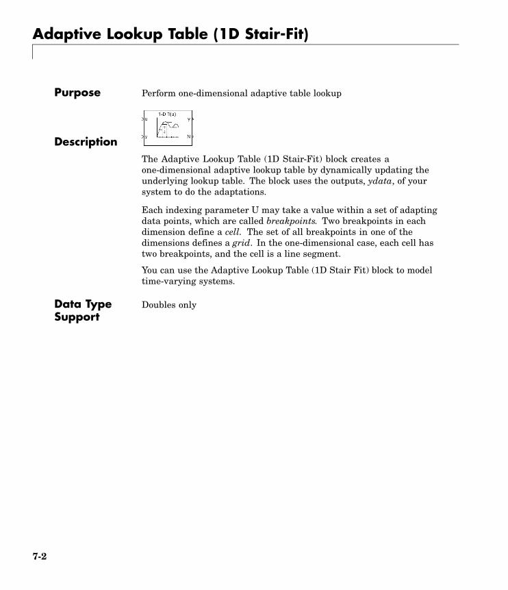
Adaptive Lookup Table (1D Stair-Fit)
Purpose Perform one-dimensional adaptive table lookup
DescriptionThe Adaptive Lookup Table (1D Stair-Fit) block creates aone-dimensional adaptive lookup table by dynamically updating theunderlying lookup table. The block uses the outputs, ydata, of yoursystem to do the adaptations.
Each indexing parameter U may take a value within a set of adaptingdata points, which are called breakpoints. Two breakpoints in eachdimension define a cell. The set of all breakpoints in one of thedimensions defines a grid. In the one-dimensional case, each cell hastwo breakpoints, and the cell is a line segment.
You can use the Adaptive Lookup Table (1D Stair Fit) block to modeltime-varying systems.
Data TypeSupport
Doubles only
7-2

Adaptive Lookup Table (1D Stair-Fit)
DialogBox
First input (row) breakpoint setThe vector of values containing possible block input values. Theinput vector must be monotonically increasing.
Make initial table an inputSelecting this check box forces the Adaptive Lookup Table (1DStair-Fit) block to ignore the Table data (initial) parameter.Instead, a new port appears with Tin next to it. Use this portto input table data.
Table data (initial)The initial table output values. This vector must be of size N-1,where N is the number of breakpoints.
7-3

Adaptive Lookup Table (1D Stair-Fit)
Table numbering dataNumber values assigned to cells. This vector must be the samesize as the table data vector, and each value must be unique.
Adaptation methodChoose Sample mean or Sample mean with forgetting. Samplemean averages all the values received within a cell. Sample meanwith forgetting gives more weight to the new data. How muchweight is determined by the Adaptation gain parameter.
Adaptation gain (0 to 1)A number between 0 and 1 that regulates the weight given to newdata during the adaptation. A 0 means short memory (last databecomes the table value), and 1 means long memory (average alldata received in a cell).
Make adapted table an outputSelecting this check box creates an additional output port for theadapted table.
Add adaptation enable/disable/reset portAdd an input port that enables, disables, or resets the adaptivelookup table. 0 = disable; 1 = enable; 2 = reset to initial table data.
Add cell lock enable/disable portA port that provides the means for updating only specified cellsduring a simulation run. 0 = unlock; 1 = lock current cell.
Action for out-of-range inputIgnore or Adapt by extrapolating beyond the extreme breakpoints.
7-4

Adaptive Lookup Table (2D Stair-Fit)
Purpose Perform two-dimensional adaptive table lookup
DescriptionThe Adaptive Lookup Table (2D Stair-Fit) block creates atwo-dimensional adaptive lookup table by dynamically updating theunderlying lookup table. The block uses the outputs (ydata) of yoursystem to do the adaptations.
Each indexing parameter U may take a value within a set of adaptingdata points, which are called breakpoints. Two breakpoints in eachdimension define a cell. The set of all breakpoints in one of thedimensions defines a grid. In the two-dimensional case, each cell hasfour breakpoints and is a flat surface.
You can use the Adaptive Lookup Table (2D Stair-Fit) block to modeltime-varying systems.
7-5

Adaptive Lookup Table (2D Stair-Fit)
DialogBox
First input (row) breakpoint setThe vector of values containing possible block input values for thefirst input variable. The first input vector must be monotonicallyincreasing.
Second input (column) breakpoint setThe vector of values containing possible block input values forthe second input variable. The second input vector must bemonotonically increasing.
Make initial table an inputSelecting this check box forces the Adaptive Lookup Table (2DStair-Fit) block to ignore the Table data (initial) parameter.
7-6

Adaptive Lookup Table (2D Stair-Fit)
Instead, a new port appears with Tin next to it. Use this portto input table data.
Table data (initial)The initial table output values. This 2-by-2 matrix must be of size(n-1)-by-(m-1), where n is the number of first input breakpointsand m is the number of second input breakpoints.
Table numbering dataNumber values assigned to cells. This matrix must be the samesize as the table data matrix, and each value must be unique.
Adaptation methodChoose Sample mean or Sample mean with forgetting. Samplemean averages all the values received within a cell. Sample meanwith forgetting gives more weight to the new data. How muchweight is determined by the Adaptation gain parameter.
Adaptation gain (0 to 1)A number from 0 to 1 that regulates the weight given to newdata during the adaptation. A 0 means short memory (last databecomes the table value), and 1 means long memory (average alldata received in a cell).
Make adapted table an outputSelecting this check box creates an additional output port for theadapted table.
Add adaptation enable/disable/reset portAdd an input port that enables, disables, or resets the adaptivelookup table.
Add cell lock enable/disable portA port that provides the means for updating only specified cellsduring a simulation run.
Action for out-of-range inputIgnore or Adapt by extrapolating beyond the extreme breakpoints.
7-7

Adaptive Lookup Table (nD Stair-Fit)
Purpose Create adaptive lookup table of arbitrary dimension
DescriptionThe Adaptive Lookup Table (nD Stair-Fit) block creates an adaptivelookup table of arbitrary dimension by dynamically updating theunderlying lookup table. The block uses the outputs of your system todo the adaptations.
Each indexing parameter may take a value within a set of adapting datapoints, which are called breakpoints. Breakpoints in each dimensiondefine a cell. The set of all breakpoints in one of the dimensions definesa grid. In the n-dimensional case, each cell has two n breakpoints andis an (n-1) hypersurface.
You can use the Adaptive Lookup Table (nD Stair-Fit) block to modeltime-varying systems.
7-8

Adaptive Lookup Table (nD Stair-Fit)
DialogBox
Number of table dimensionsThe number of dimensions for the adaptive lookup table.
Table breakpoints (cell array)A set of one-dimensional vectors that contains possible blockinput values for the input variables. Each input row must bemonotonically increasing, but the rows do not have to be the samelength. For example, if the Number of table dimensions is 3,you can set the table breakpoints as follows:
{[1 2 3], [5 7], [1 3 5 7]}
7-9

Adaptive Lookup Table (nD Stair-Fit)
Make initial table an inputSelecting this check box forces the Adaptive Lookup Table (nDStair-Fit) block to ignore the Table data (initial) parameter.Instead, a new port appears with Tin next to it. Use this portto input table data.
Table data (initial)The initial table output values. This (n-D) array must be of size(n-1)-by-(n-1) ... -by- (n-1), (D times), where D is the number ofdimensions and n is the number of input breakpoints.
Table numbering dataNumber values assigned to cells. This vector must be the samesize as the table data array, and each value must be unique.
Adaptation methodChoose Sample mean or Sample mean with forgetting. Samplemean averages all the values received within a cell. Sample meanwith forgetting gives more weight to the new data. How muchweight is determined by the Adaptation gain parameter.
Adaptation gain (0 to 1)A number from 0 to 1 that regulates the weight given to newdata during the adaptation. A 0 means short memory (last databecomes the table value), and 1 means long memory (average alldata received in a cell).
Make adapted table an outputSelecting this check box creates an additional output port for theadapted table.
Add adaptation enable/disable/reset portAdd an input port that enables, disables, or resets the adaptivelookup table.
Add cell lock enable/disable portA port that provides the means for updating only specified cellsduring a simulation run.
Action for out-of-range inputIgnore or Adapt by extrapolating beyond the extreme breakpoints.
7-10

8
Functions — AlphabeticalList
spetool

spetool
Purpose Open Simulink Parameter Estimation GUI
Syntax spetool('modelname')
Description spetool('modelname') opens Simulink Parameter Estimation GUI forthe Simulink model with the name modelname.
See Also For more information about using Simulink Parameter Estimation GUI,see Chapter 1, “Getting Started”.
8-2

Index
IndexAadaptive lookup tables 5-2adding data sets 1-20
Ccommand-line estimation 6-3Controls and Estimation Tools Manager 1-8
Ddata
detrending 3-14exclusion 3-5filtering 3-14preprocessing 3-3
Data Import dialog box 1-12data sets
adding 1-20detrending data 3-14display options for estimation 1-24
Eestimation
display options 1-24example of command-line estimation 6-5from the command line 6-3running 1-28selecting parameters 1-14selecting states 1-16setting up a project 1-20
excluding data 3-5
Ffiltering data 3-14
Iimporting
initial conditions 1-13transient data 1-10
initial conditionsexample of estimating 2-4importing 1-13
initial guesses 1-17
Llookup tables
adaptive 5-2
Mmultiple projects and tasks 4-2
Ooptimization
setting options for 1-41
Pparameters
selecting for estimation 1-14specification of 1-22
preprocessing data 3-3projects
definition of 1-6saving 4-3
Rrunning an estimation 1-28
Ssaving projects 4-3selecting views 1-25setting options
for optimization 1-41
Index-1
Index
for simulation 1-41upper/lower bounds 1-17
simulationsetting options for 1-41
specifying parameters 1-22states
selecting for estimation 1-16
Ttransient data
importing 1-10
Uupper/lower bounds
setting 1-17
Vviews
selecting 1-25
Index-2