SIMULATION TECHNIQUES TO MODEL FLOW AND TRANSPORT AT THE PORE-SCALE

4 T H CARGESE SUMMER SCHOOL

CARGESE, JULY 4, 2018

Cyprien Soulaine

2

Outline

● Pore-scale modeling,

● Derivation of Navier-Stokes equations,

● Properties of Navier-Stokes equations,

● Numerical approaches to solve the flow at the pore-scale,

● Simulation examples,

● Two-phase flow at the pore-scale.

3

Continuum mechanicsStatistical mechanics

Navier-Stokes Darcy

Multi-scale modeling

(Adapted from Buchgraber 2012)

4

Discret vs continuum

for every point of the domain

fluid OR solid fluid AND solid

5

Digital Rock Physics

(source: GeoDict)

6

Single-phase flows at the pore-scale

● Water seeded with micro-particles to visualize the flow in the pore-space*,

● The particle trajectories are not random and are deterministic.

* Roman et al. Particle velocimetry analysis of immiscible two-phase flow in micromodels, Advances in Water Resources 2016

7

The Navier-Stokes equations● The flow motion obeys the continuum mechanics conservation laws for

fluid,

● These laws are derived from mass and momentum balance in a control volume,

● The Navier-Stokes equations are made of:

● A continuity equation,

● A momentum equation,

● Boundary conditions at the solid surface.

λ = mean free path

λ << r

8

Mass balance equation

= fluid density mass of fluid=

control volume

Variation of mass in the control volume

Mass fluxes coming and going out the control volume

For an incompressible fluid (most of the liquids):

9

Cauchy momentum equation

Conservation of momentum obtained from Newton’s second law of motion (the variation of momentum and the sum of forces balance each other):

Body forces = gravity, magnetic of electric fields…

Surface forces = forces responsible for the deformation of the control volume

= fluid momentum

10

Shear stress for Newtonian fluids

Cauchy stress tensor quantifies the change in shape and/or size of the control volume,

For Newtonian fluid, the viscous stress is proportional to the strain rate (the rate at which the fluid is being deformed),

11

Navier-Stokes momentum equation

In an Eulerian frame, the combination of Cauchy’s law and Cauchy stress tensor gives the Navier-Stokes momentum equation,

For slow flow, the inertial term is negligible compared with the dissipative viscous force and Navier-Stokes becomes the Stokes equation,

Stokes is a particular case of Navier-Stokes, which means that all Navier-Stokes solvers are also valid for Stokes without any modification!

12

Boundary conditions at the solid surface

13

The Navier-Stokes equations: summary

● Mass balance equation,

● Momentum balance equation,

● No slip condition at the solid surface,

14

Different flow regimes (past a cylinder)

Creeping flow regime (Re<1): the flow is governed by the viscous effects only and the streamlines embrace the solid structure. The flow is modeled by the Stokes equations. Most of the time, we are in this situation.

The inertia effects distort the streamlines and flow recirculations are generated downstream the obstacles. The flow is modeled by the laminar Navier-Stokes equations.

At very high Reynolds numbers, turbulence effects emerge. The flow is modeled by turbulent Navier-Stokes equations (RANS, LES...)

15

Recirculating motion in Stokes flows

● Cavities/ Roughness2

● Space between two grains1

1Caltagirone, Physique des écoulements continus, 2013 2Higdon, Stokes flow in arbitrary two-dimensional domains: shear flow over ridges and cavities, Journal of Fluid Mechanics, 1985, 159, 195-226

16

Analytical solution: flow between two parallel plates

W and L assume to be large enough so

The Stokes problem in Cartesian coordinates reads

When volume averaging the velocity profile:

Parabolic profile

Hele-Shaw equation

17

Analytical solution: flow in a micro-tube

L assumes to be long enough so the flow does not depend on z. Moreover, it is invariant by rotation and is carried by z only:

Due to the geometry, it is natural to use cylindrical coordinates.

The Stokes problem in cylindrical coordinates reads

When volume averaging the velocity profile:

Parabolic profile

Hagen-Poiseuille law:

18

How to solve flows in complex porous structures?

Acquisition of the image (micro-CT ...)

Direct Numerical Simulation (DNS)

Pore-network modeling (PNM)

Segmentation in fluid and solid

Source: Blunt et al. (2013)

19

Pore Network Modeling

with

(cf. Poiseuille flow in a microtube)Due to the mass conservation, for all pores P:

● Very easy to program ● Can compute relatively large domains (up to cm)

● Need more sophisticated models to be more representative of the actual geometry (bonds are not always cylindrical).

● It is not a tool to investigate the physics, the results will depend on the input…● Still needs some research to the extension for multiphase

For a cylindrical bond of radius ri and length L

i that relates the nodes P and i, the mass flow rate is

bond

nodepore body

pore throat

solid grain

20

Direct Numerical Simulation techniques

Lattice Boltzmann Method (LBM)

● Solve the discrete Boltzmann equation instead of Navier-Stokes,

● The nature of the lattice determines the degree of freedom for the particle movement,

● Easy to program, massively parallel,● No limitation due to Knudsen number.

Direct modeling

Navier-Stokes on Eulerian grids (CFD)

● Solve Navier-Stokes equations on a Eulerian grid,

● Differential operators discretized with FVM, FDM or FEM,

● Nowadays, all the CFD softwares are efficient, robust and parallelized.

- Directly deal with the real pore structure geometry,- Can be used to investigate the physics

- More computationally expensive than PNM, - Efficient multiphase solver are still in development.

Smoothed-Particle Hydrodynamics (SPH)

● Mesh-free technique,● Fluid is divided into a set of discrete

particles,● To represent continuous variables, a

kernel defined the sphere of influence of a particle,

● Particles are tracked in time as they move in the pore-space using a Lagrangian framework.

21

Some popular CFD softwares

https://www.cypriensoulaine.com/openfoam

OpenFOAM is a general purpose open-source CFD code. OpenFOAM is written in C++ and uses an object oriented approach which makes it easy to extend. The package includes modules for a wide range of applications. It uses the finite volume method.

COMSOL Multiphysics is a finite element package for various physics and engineering application, especially coupled phenomena or multiphysics.

ANSYS Fluent is a CFD software using the finite volume method.

Another commercial CFD software.

22

Pressure-velocity coupling with projection algorithms

* Issa. Solution of the Implicitly Discretised Fluid Flow Equations by Operator-Splitting. Journal of Computational Physics, 62:40-65, 1985.** Patankar. Numerical Heat Transfer And Fluid Flow, Taylor & Francis, 1980

● The pressure and velocity equations are solved in a sequential manner using predictor-corrector projection algorithms. In OpenFOAM®, you have to choose between PISO and SIMPLE:

● PISO is not unconditionally stable and the time step is limited by a CFL condition.

● SIMPLE is an iterative procedure that under-relaxes the pressure field and velocity matrix at each iteration.

● To allow larger time steps, a combination of both algorithm is sometime proposed (PIMPLE).

● Multiphase Navier-Stokes equations are solved in the framework of the PISO solution procedure.

● Stokes momentum equation does not involve transient terms and can be solved with SIMPLE.

algorithm transient Steady-state

comments OpenFOAM solver

PISO*PIMPLE

YES YES Can be used to find the stationary solution by solving all the time steps

icoFoam, pisoFoam, pimpleFoam, interFoam, twoPhaseEulerFoam, rhoPimpleFoam...

SIMPLE** NO YES Faster than PISO to converge to the steady state

simpleFoam, rhoSimpleFoam...

● Two equations, two unknowns (pressure and velocity) but no equation for the pressure field.

and

● A pressure equation can be derived by taking the divergence of the momentum equation.

23

Application: compute the permeability of a sandstone

● Digital rock obtained from microtomography imaging,

● Grid the pore-space,

● In CFD simulations, the results may be very sensitive to the grid quality. At least 10 cells are required in each pore-throat,

● The grid quality is even more important when dealing with multiphase flow (refinement near the walls),

● Solve steady-state Stokes equations (SIMPLE algorithm with OpenFOAM).

24

Simulations in “2.5D” micromodels

Pressure Velocity

The simulation is 2D. The 3D effects are included assuming a Poiseuille profile in the depth of the micromodels and then considering Stokes flow equations averaged over the thickness, i.e. adding an Hele-Shaw correction term.

* Roman et al. Particle velocimetry analysis of immiscible two-phase flow in micromodels, Advances in Water Resources 2016

Hele-Shaw correction term

25

Physics of two-phase flow in porous media at the pore-scale

θ=150°non-wetting

θ=90° θ=7°wetting

Zhao e

t al. (

20

16

), P

NA

S

Surface tension (N/m)

Immiscible interface

Particularity of multi-phase flow

• Navier-Stokes equation in each phases

• Continuity of the tangential component of the velocity at the fluid/fluid interface

• Laplace law for a surface at the equilibrium

• Contact line dynamics at the solid surface

Surface tension is the elastic tendency of a fluid surface which makes it acquire the least surface area possible

The contact angle quantifies the wettability affinity of a solid surface by a liquid

The displacement of a wetting fluid by a non-wetting fluid (drainage) is different than the displacement of a non-wetting fluid by a wetting fluid (imbibition)

Sophie Roman (Univ of Orléans, FR)

26

CFD for two-phase flow

Wörner, Numerical modeling of multiphase flows in microfluidics and micro process engineering: a review of methods and applications , Microfluidics and Nanofluidics 2012

Source: Wörner (2012)

• The state-of-the-art simulations can not go below Ca=10-5. Otherwise spurious currents can pollute and even drive the interface propagation

• The physics of contact line dynamics is still poorly understood and can have an order one impact on the flow (Constant contact angle? Cox-Voinov model? Lubrication theory for thin film? ).

• Solve the flow on large and complex domains.

• How to validate this numerical models?

ChallengesSimulation methods

27

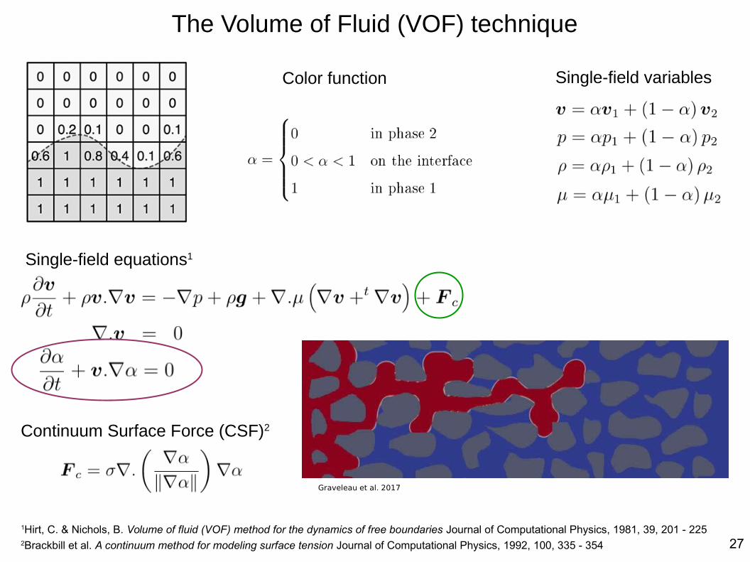
The Volume of Fluid (VOF) technique

Color function Single-field variables

Single-field equations1

1Hirt, C. & Nichols, B. Volume of fluid (VOF) method for the dynamics of free boundaries Journal of Computational Physics, 1981, 39, 201 - 225 2Brackbill et al. A continuum method for modeling surface tension Journal of Computational Physics, 1992, 100, 335 - 354

Continuum Surface Force (CSF)2

Graveleau et al. 2017

28

Thank you for your attention!

www.cypriensoulaine.com