Embed Size (px)
Citation preview

Applied Mathematical Sciences, Vol. 5, 2011, no. 57, 2807 - 2818
Simulation Study: Introduction of Imputation
Methods for Missing Data in Longitudinal Analysis
Michikazu Nakai
Innovation Center for Medical Redox Navigation
Kyushu University, Fukuoka, 812-8582, Japan
Abstract
Missing data are vital subject to perform a proper longitudinal analysis.
Some just ignore and discard all missing data to have complete dataset.
However, it can result in a very substantial loss of information. Therefore,
it is important to comprehend imputation methods of handling missing
data. This paper discusses four common imputation methods for
longitudinal analysis. Then, using simulation study, comparison and
accuracy of these imputation methods are illustrated. The final section
provides summary.
Mathematical Subject Classification: 62-07, 62H15, 62Q05
Keywords: Longitudinal analysis, Imputation, Missing data
1 Introduction
Longitudinal studies are characterized by a sample design which specifies
repeated observations on the same experimental unit [6]. Failure to obtain a full
set of observations on a given unit results in incomplete data and/or unbalanced

2808 M. Nakai
designs. There are a variety of reasons data would be missing. For example, data
might be missing because some participants were offended by certain questions
on a survey (participant characteristics), or because a study required too much of
the participant’s time (design characteristics), or because those who were the
sickest were unable to complete the more burdensome aspects of the study
(participant and design characteristics) [10]. Such missing values are a common
problem in longitudinal studies.
The development of imputation methods for analyzing data with missing data
has been an active area of research. Recent researches have already shown that
the distinct and characteristics of missing mechanisms [1,4,5,8,16]. Nonetheless,
there is not a lot of guidance about rules of applying imputation methods. Since
there is no clear rules exist regarding how much is too much missing data [11],
researchers don’t consider missingness as a huge problem. In the result, some
researchers tend to perform exactly the same imputation to fill in such missing
values without consideration. However, it is not always smart idea to convey a
particular method every time to estimate parameters in longitudinal analysis
because missing data can have important consequences on the
amount/percentage and pattern of missing data, the selection of appropriate
missing data handling methods and the interpretation of research results. Hence,
we must examine missing data carefully and adjust the proper imputation
method.
This paper focuses on comparison among selected imputation methods and
provides characteristics of imputation methods. The first section states an
overview of missing mechanism and imputation methods. The subsequent
section presents a simulation study to apply imputation methods and explains
advantages and disadvantages of each imputation. The final section concludes
with some remarks.
2 Method
2.1 Missing Mechanism
— Missing at Random
— Missing Completely at Random
— Not Missing at Random
—

Imputation methods for missing data in longitudinal analysis 2809
There are three different missing mechanisms developed by Rubin [15] and
each mechanism has unique characteristics to recognize before analyzing and
handling missing data effectively. The word “mechanism” is being used because
it specifies the structural relationships between the condition of the data that are
missing and the observed and/or missing values of the other variables in the data
without specifying the hypothetical underlying cause of these relationships. Use
of the word “mechanism”, therefore, does not imply that we necessarily know
anything about how the missing data come to be missing [10].
The first mechanism is called as Missing at Random (MAR). Under MAR,
the probability of missingness depends on the observed data, but not the
unobserved data. The special case of MAR is the second mechanism, called
Missing Completely at Random (MCAR). Under MCAR, the probability of
missingness is independent of both observed data and unobserved data. The last
mechanism is called Not Missing at Random (NMAR). Under NMAR, the
probability of missingness depends on both observed data and unobserved data.
It is sometimes referred to NMAR as Missing at Not Random (MANR) or
Missing Not at Random (MNAR), depending on the author’s preference. Since
the probability of missing data is related to at least some unobserved data,
NMAR is often referred as non-ignorable, which implies to the fact that missing
data mechanism cannot be ignored. More detailed explanations for each
mechanism are referred to [8,12,13].
2.2 Imputation
— Complete Case method
— Last Observation Carried Forward method
— Mean Imputation method
— Multiple Imputation method
A primary method of handling missing data is Complete Case method. The
method is simply to omit all case with missing data at any measurement
occasion, and this is a default method in most statistical packages to treat
missing data. The advantage of its method is that no special computational
methods are required and it can be used for any kind of statistical analysis.
However, the research has already shown the method requires MCAR for
2810 M. Nakai
unbiased estimation [1,4,8,10].
One of the most widely used imputation methods in longitudinal analysis is
Last Observation Carried Forward (LOCF) method. The method is for every
missing data to be replaced by the last observed value from the same subject.
Although the assumption of missing values is MAR, a recent research has
shown that LOCF method creates bias even in MCAR; Additionally, this method
does not give a valid analysis if the missing mechanism is anything other than
MCAR [7].
Next method is Mean Imputation method. The method assumes that the mean
of the variable is the best estimate for any observation that has missing data for
the variable. That is, mean of the non-missing data is used in place of the
missing data. Even though this strategy is simple to impute, it can severely
distort the distribution for its variable, including underestimation of the standard
deviation. This method also assumes missing mechanism to be MCAR.
The most popular imputation method of handling missing data is Multiple
Imputation (MI) method in which replaces each missing item with two or more
acceptable values representing a distribution of possibilities. The advantage of
its method is that once the imputed dataset has been generated, the analysis can
be carried out using procedures in virtually any statistical packages. However,
there are some disadvantages. Missing data individuals are allowed to have
distinct probability which indicates that individual variation is ignored.
Furthermore, the uncertainty inherent in missing data is ignored because the
analysis does not distinguish between the observed and imputed values. Some
important references in the field can be found in [8,13,14,17].
3. Simulation Study
For a dataset, suppose repeated measurements 𝑌𝑖𝑡(𝑖 = 1, ⋯ , 100; 𝑡 = 1, ⋯ ,5)
are generated from a multivariate normal distribution with mean response
𝐸(𝑌𝑖𝑡) = 𝛽0 + 𝛽1𝑡 where 𝛽0 = intercept, 𝛽1 = slope and correlation =
𝜌|𝑠−𝑡|for 𝜌 ≥ 0, then simulated N=200 different random longitudinal datasets in
SAS®. The variance at each occasion is assumed to be constant over time, while
the correlations have a first-order autoregressive (AR(1)) pattern with positive
coefficient [4]. Assuming that the first occasion was fully observed, simple

Imputation methods for missing data in longitudinal analysis 2811
random sampling without replacement was used to make MCAR datasets and to
test0%, 10%, 20%, 30% and 50% at time point 1, 2, 3, 4, 5 cases of missing
datasets, respectively. The experiment itself consists of mean of the 200
empirical means (1000 for MI) and Mean Square Error (MSE) from a fitted
mean 𝐸(𝑌𝑖𝑡). In addition, normality Shapiro-Wilk test is performed to each
imputation method at each time point and Analysis of Variance (ANOVA) test is
conducted to verify the significance whether means are different between
original dataset and imputed dataset with α = 0.05 level. Multiple comparison
with Turkey procedure is used for mean comparisons. If normality test fails, its
imputation excludes from comparison. At last, two different slope values (0.1
and 2) are tested to investigate the effectiveness for imputations. The default
numbers for each parameters are following: ρ = 0.7 , 𝜎2 = 1 , 𝛽0 = 10 ,
and 𝛽1 = 0.1.
This simulation compares three tables for imputation methods in longitudinal
analysis. Table1 shows the default condition for each time point. Table2 explores
relationship of correlation coefficient and missingness, which justifies whether a
small correlation among time points reflects accuracy of imputation methods. At
last, Table3 considers whether big variables estimate any differences of each
imputation.
The computation was mainly carried out using the computer facilities at
Research Institute for Information Technology, Kyushu University.
4 Result
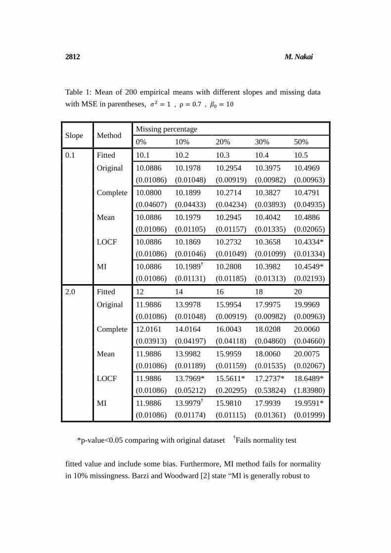
At first, Table1 yields that all cases in Complete Case method are not rejected
with α = 0.05 level and normality tests are clear. Comparing with other
methods, MSE may be higher which explains bias appearance. Mean Imputation
method does not seem to present any disadvantage elements in Table1. LOCF
method already imputes poorly in slope = 2. However, in slope = 0.1 , its
method is accurate up to 30% missingness. One element to notice in LOCF
method is that MSE from 20% missingness in slope = 2starts to increase
enormously. It is obvious that imputed observations arise far from a
2812 M. Nakai
Table 1: Mean of 200 empirical means with different slopes and missing data
with MSE in parentheses, 𝜎2 = 1 , ρ = 0.7 , 𝛽0 = 10
Slope Method Missing percentage
0% 10% 20% 30% 50%
0.1 Fitted 10.1 10.2 10.3 10.4 10.5
Original 10.0886
(0.01086)
10.1978
(0.01048)
10.2954
(0.00919)
10.3975
(0.00982)
10.4969
(0.00963)
Complete 10.0800
(0.04607)
10.1899
(0.04433)
10.2714
(0.04234)
10.3827
(0.03893)
10.4791
(0.04935)
Mean 10.0886
(0.01086)
10.1979
(0.01105)
10.2945
(0.01157)
10.4042
(0.01335)
10.4886
(0.02065)
LOCF 10.0886
(0.01086)
10.1869
(0.01046)
10.2732
(0.01049)
10.3658
(0.01099)
10.4334*
(0.01334)
MI 10.0886
(0.01086)
10.1989†
(0.01131)
10.2808
(0.01185)
10.3982
(0.01313)
10.4549*
(0.02193)
2.0 Fitted 12 14 16 18 20
Original 11.9886
(0.01086)
13.9978
(0.01048)
15.9954
(0.00919)
17.9975
(0.00982)
19.9969
(0.00963)
Complete 12.0161
(0.03913)
14.0164
(0.04197)
16.0043
(0.04118)
18.0208
(0.04860)
20.0060
(0.04660)
Mean 11.9886
(0.01086)
13.9982
(0.01189)
15.9959
(0.01159)
18.0060
(0.01535)
20.0075
(0.02067)
LOCF 11.9886
(0.01086)
13.7969*
(0.05212)
15.5611*
(0.20295)
17.2737*
(0.53824)
18.6489*
(1.83980)
MI 11.9886
(0.01086)
13.9979†
(0.01174)
15.9810
(0.01115)
17.9939
(0.01361)
19.9591*
(0.01999)
*p-value<0.05 comparing with original dataset †Fails normality test
fitted value and include some bias. Furthermore, MI method fails for normality
in 10% missingness. Barzi and Woodward [2] state “MI is generally robust to

Imputation methods for missing data in longitudinal analysis 2813
departures from normality and generally to model misspecification when the
amounts of missing data are not large”, which matches the result in this
simulation. MI method seems to have difficulty to evaluate missing data for
50% missingness in both slopes.
Table2 inquires the difference for correlation coefficient among time points.
Both Complete Case method and Mean Imputation method do not recognize
much distinction with Table1. That is, both methods do not affect correlation
coefficient for imputation. However, LOCF method shows inadequate for
normality from 30% missingness in slope = 2. Since its method imputes last
values before missing values, as missingness and slope become larger, the
imputed values tend to be smaller than assumed values. That is, the distribution
itself would more likely to be skewed. Therefore, when slope and missingness
increase with low correlation, normality test for LOCF method tends to fail.
Besides, normality for MI method is not stable in slope = 2.
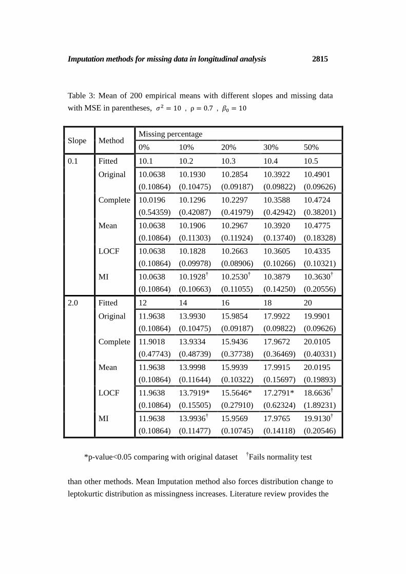
Table3 increases variance from 𝜎2 = 1 to 𝜎2 = 10. Apparently, observations
are spread so that MSE values also have enlarged compared with Table1 and
Table2.Moreover, large variance influences MSE for Complete Case method
which jumps up more than twice of MSE from original dataset. However, the
mean values do not appear the statistical difference from original mean. And, the
disadvantages of losing sample size and power do not seem to appear in this
simulation. Mean Imputation method also does not emerge much disadvantage
of underestimating standard deviation by comparing mean and MSE. LOCF
method imputes efficiently in slope = 0.1 while statistical difference presents
in slope = 2. MI method demonstrates lack of accuracy for normality even
in slope = 0.1.
5 Discussion
In this paper, we have reviewed missing mechanism and imputation methods,
examined the consequences of missing data in longitudinal studies and
compared different imputation methods for effectiveness. To summarize the
simulation results, Complete Case method and Mean Imputation method yield
reasonable mean values to accept null hypothesis of analysis. Moreover,
Complete Case method handles well if missingness is less than 15% [17].

2814 M. Nakai
Table 2: Mean of 200 empirical means with different slopes and missing data
with MSE in parentheses, 𝜎2 = 1 , ρ = 0.2 , 𝛽0 = 10
Slope Method Missing percentage
0% 10% 20% 30% 50%
0.1 Fitted 10.1 10.2 10.3 10.4 10.5
Original 10.0871
(0.01123)
10.2028
(0.01087)
10.2964
(0.00951)
10.3997
(0.01004)
10.4977
(0.01004)
Complete 10.0759
(0.05433)
10.2069
(0.03903)
10.2734
(0.04334)
10.4099
(0.05384)
10.5003
(0.03284)
Mean 10.0871
(0.01123)
10.2059
(0.01197)
10.2948
(0.01079)
10.4024
(0.01486)
10.4932
(0.01830)
LOCF 10.0871
(0.01123)
10.1899
(0.01014)
10.2718
(0.01037)
10.3653
(0.01088)
10.4283*
(0.01484)
MI 10.0871
(0.01123)
10.2058
(0.01231)
10.2746
(0.01290)
10.3961
(0.01857)
10.4337*
(0.02906)
2.0 Fitted 12 14 16 18 20
Original 11.9871
(0.01123)
14.0028
(0.01087)
15.9964
(0.00951)
17.9997
(0.01004)
19.9977
(0.01004)
Complete 11.9954
(0.04473)
14.0039
(0.04633)
15.9790
(0.04806)
18.0177
(0.04108)
19.9984
(0.04150)
Mean 11.9871
(0.01123)
14.0052
(0.01237)
15.9892
(0.01243)
17.9983
(0.01260)
19.9920
(0.02102)
LOCF 11.9871
(0.01123)
13.8019*
(0.05050)
15.5587*
(0.20529)
17.2804†
(0.53001)
18.6388†
(1.86614)
MI 11.9871
(0.01123)
14.0047
(0.01346)
15.9678†
(0.01560)
17.9941
(0.01686)
19.9293†
(0.03067)
*p-value<0.05 comparing with original dataset †Fails normality test
However, as stated, Complete Case method has disadvantage of losing sample
size and power. In addition, MSE in Complete Case method shows higher values
Imputation methods for missing data in longitudinal analysis 2815
Table 3: Mean of 200 empirical means with different slopes and missing data
with MSE in parentheses, 𝜎2 = 10 , ρ = 0.7 , 𝛽0 = 10
Slope Method Missing percentage
0% 10% 20% 30% 50%
0.1 Fitted 10.1 10.2 10.3 10.4 10.5
Original 10.0638
(0.10864)
10.1930
(0.10475)
10.2854
(0.09187)
10.3922
(0.09822)
10.4901
(0.09626)
Complete 10.0196
(0.54359)
10.1296
(0.42087)
10.2297
(0.41979)
10.3588
(0.42942)
10.4724
(0.38201)
Mean 10.0638
(0.10864)
10.1906
(0.11303)
10.2967
(0.11924)
10.3920
(0.13740)
10.4775
(0.18328)
LOCF 10.0638
(0.10864)
10.1828
(0.09978)
10.2663
(0.08906)
10.3605
(0.10266)
10.4335
(0.10321)
MI 10.0638
(0.10864)
10.1928†
(0.10663)
10.2530†
(0.11055)
10.3879
(0.14250)
10.3630†
(0.20556)
2.0 Fitted 12 14 16 18 20
Original 11.9638
(0.10864)
13.9930
(0.10475)
15.9854
(0.09187)
17.9922
(0.09822)
19.9901
(0.09626)
Complete 11.9018
(0.47743)
13.9334
(0.48739)
15.9436
(0.37738)
17.9672
(0.36469)
20.0105
(0.40331)
Mean 11.9638
(0.10864)
13.9998
(0.11644)
15.9939
(0.10322)
17.9915
(0.15697)
20.0195
(0.19893)
LOCF 11.9638
(0.10864)
13.7919*
(0.15505)
15.5646*
(0.27910)
17.2791*
(0.62324)
18.6636†
(1.89231)
MI 11.9638
(0.10864)
13.9936†
(0.11477)
15.9569
(0.10745)
17.9765
(0.14118)
19.9130†
(0.20546)
*p-value<0.05 comparing with original dataset †Fails normality test
than other methods. Mean Imputation method also forces distribution change to
leptokurtic distribution as missingness increases. Literature review provides the
2816 M. Nakai
comparison between Complete Case method and Mean Imputation method, and
states that Mean Imputation method is more accurate than Complete Case
method [14]. LOCF method often fails normality test especially when
missingness increases and slope is large. Lane [7] points out that LOCF method
gives some bias even when dataset is MCAR. Simulation results show that
LOCF method is fairly effective to fill in missing data when slope is small.
However, when slope gets larger, LOCF method tend to lose accuracy from 10%
missingness. This consequence agrees with previous literature [9]. Even though
LOCF method seems to be inapplicable method for handling missing data,
Engels and Diehr [3] compare 14 methods of imputing missing data and
recommend LOCF method as the best estimation for imputation method. Finally,
literature explains MI method is the most conclusive technique to impute
missing data [8,16]. According to this simulation, MI method performs
deficiency in accuracy for normality.
In overall, Complete Case method concludes good imputation method with
condition of small missing percentage and large sample size to improve its
disadvantages. As Allison refers, Complete Case method “is not a bad method
for handling missing data” [1].When losing sample sizes is concerned under
same situation, then Mean Imputation method is recommended. When values at
each time point are fairly small, then LOCF method delivers appropriate
imputed value. However, its method is not recommended when values at each
time point are large. MI method tends to impute poorly for normality. After
getting over the condition, MI method is quite reasonable method considering
improvement in future research. In further discussion, smaller missing
percentages such as 5% or 15% are expected to investigate the detail of
efficiency for each imputation methods. Other covariate structures such as
compound symmetric or unstructured model can be examined applying
consistent simulation study to compare.
References
[1] P. Allison, Missing Data, Sage Publications Inc, California, 2001

Imputation methods for missing data in longitudinal analysis 2817
[2] F. Barzi and M. Woodward, Imputation of Missing Values in Practice:
Results from Imputations of Serum Cholesterol in 28 Cohort Studies, American
Journal of Epidemiology, 160 (2004), 34-45
[3] J.M. Engels and P. Diehr, Imputation of missing longitudinal data: a
comparison of methods, Journal of Clinical Epidemiology, 56(2003), 968-976
[4] G.M. Fizmaurice, N.M, Laird, and J.H. Ware, Applied Longitudinal Analysis,
Wiley, New York, 2004
[5] D. Hedeker and R.D. Gibbons, Longitudinal Data Analysis, Wiley, New York,
2006
[6] N.M. Laird, Missing Data in Longitudinal Studies, Statistics in Medicine, 7
(1988), 305-315
[7] P. Lane, Handling drop-out in longitudinal clinical trial: a comparison of the
LOCF and MMRM approaches, Pharmaceutical Statistics, 7 (2008),93-106
[8] R.J.A Little and D.B Rubin, Statistical Analysis with Missing Data, second
edition, Wiley, New York, 2002
[9] R. Liu and V. Ramakrishnan, Application of Multiple Imputation in Analysis
of Data from Clinical Trials with Treatment Related Dropouts, Communications
in Statistics-Theory and Methods, 38 (2009), 3666-3677
[10] P.E. McKnight, K.M, McKnight, S.Sidani, A.J. Figueredo, Missing Data-A
Gentle Introduction, The Guilford Press, New York, 2007
[11] C.M.Musil, C.B.Warner,P.K.Yobas, and S.L.Jones, A comparison of
imputation techniques for handling missing data, Western Journal of Nursing
Research, 24 (2002), 815-829
[12] W.R. Myers, Handling Missing Data in Clinical Trial: An Overview, Drug

2818 M. Nakai
Information Journal, 34 (2000), 525-533
[13] M. Nakai and W. Ke, Review of the Methods for Handling Missing Data in
Longitudinal Data Analysis, International Journal of Mathematical Analysis,
5(1) (2011), 1-13
[14] P.L. Roth, Missing data: A Conceptual Review For Applied
Psychologists,47(3) (1994),537-560
[15] D. B. Rubin, Inference and Missing Data, Biometrika, 63(1976), 581-592
[16] J.L. Schafer, Analysis of Incomplete Multivariate Data, Chapman &
Hall/CRC, Florida, 1997
[17] K. Strike, K.E. Eman, and N. Madhavji, Software Cost Estimation with
Incomplete Data, 27(10) (2001), 890-908
Received: February, 2011