1

NTNU Fakultet for naturvitenskap og teknologi

Norges teknisk-naturvitenskapelige Institutt for kjemisk prosessteknologi

universitet

SPECIALIZATION PROJECT SPRING 2009

TKP 4555

PROSJECT TITLE:

SIMULATION, OPTIMAL OPERATION AND SELF

OPTIMISATION OF TEALARC LNG PLANT

by

MBA, EMMANUEL ORJI

Supervisor for the project:

PROF SIGURD SKOGESTAD Date: 09-12-2009

2

CONTENTS

ACKNOWLEDGEMENT .......................................................................................................... 4

ABSTRACT ............................................................................................................................. 5

1.0. INTRODUCTION ............................................................................................................. 6

1.1 LIQUEFACTION OF NATURAL GAS ................................................................................ 6

1.2 LNG VALUE CHAIN ....................................................................................................... 6

1.3 LIQUEFACTION PROCESSES .......................................................................................... 7

1.4 OBJECTIVE ................................................................................................................... 8

2. LIQUEFICATION CYCLE ...................................................................................................... 9

2.1. CLASSIFICATION OF NATURAL GAS LIQUEFACTION PROCESSES ................................. 10

2.2 THERMODYNAMICS OF LIQUEFACTION CYCLE ............................................. 11

2.3 EXERGY ANALYSIS OF LNG CYCLE ............................................................................... 14

3.0 SELECTED THEORIES ON CONTROL STRUCTURE DESIGN ............................................... 15

3.1. DEGREES OF FREEDOM ANALYSIS FOR OPTIMISATION ....................................... 16

3.2OPTIMISATION............................................................................................................ 17

3.2.1OPTIMIZATION METHOD IN UNISIM ................................................................................. 17

3.3. OPTIMAL OPERATION ............................................................................................... 18

3.4 WHAT TO CONTROL? (SELF OPTIMISATION CONTROL) .............................................. 19

3.4.1 SELF OPTIMISING CONTROL .................................................................................... 19

3.5. SELECTION OF CONTROL VARIABLES ......................................................................... 22

3.5.1. SELECTION OF CONTROL VARIABLE C BY MINIMUM SINGULAR VALUE RULE .................. 23

3.5.2. SELECTION OF CONTROL VARIABLE C BY EXACT LOCAL METHOD .................................... 23

3.5.3. SELECTION OF CONTROL VARIABLE C BY MEASUREMENT COMBINATION METHOD ....... 24

4.0 MODELLING AND SIMULATION OF TEALARC LNG PROCESS PLANT .............................. 26

4.1 PROCESS DESCRIPTION .............................................................................................. 26

4.1.1PRE-COOLING CYCLE ........................................................................................................ 26

4.1.2 LIQUEFACTION CYCLE ...................................................................................................... 27

4.2 MODELLING AND SIMULATION OF THE UNIT OPERATIONS ........................................ 28

4.2.1LNG HEAT EXCHANGERS................................................................................................... 28

4.2.2 COMPRESSOR ................................................................................................................. 29

4.2.3 SW COOLERS ................................................................................................................... 30

3

4.2.4 VALVES............................................................................................................................ 30

4.3 SPECIFICATIONS MADE FOR THE MODELLING AND SIMULATION OF THE ENTIRE PLANT

........................................................................................................................................ 31

5.0 IMPLEMENTATION OF SELF OPTIMISING CONTROL ..................................................... 33

5.1OPTIMISING THE LIQUEFACTION SECTION .................................................................. 33

5.1.1 DEFINE OBJECTIVE FUNCTION ......................................................................................... 33

5.1.2DEGREES OF FREEDOM FOR OPERATION .......................................................................... 34

5.1.3CONSTRAINTS .................................................................................................................. 34

5.1.4DISTURBANCES ................................................................................................................ 34

5.2 OPTIMISING THE PRE-COOLING SECTION ................................................................... 35

5.2.1OBJECTIVE FUNCTION ...................................................................................................... 35

5.2.2DEGREES OF FREEDOM FOR OPERATION .......................................................................... 35

5.2.3 CONSTRAINTS ........................................................................................................... 35

5.2.4 DISTURBANCES ............................................................................................................... 35

6.0 OPTIMISATION RESULTS AND DISCUSSIONS ................................................................ 36

6.1 NOMINAL OPTIMUM RESULT FOR LIQUEFACTION PLANT .......................................... 36

6.2 ACTIVE CONSTRAINTS ........................................................................................................ 36

6.3 OPTIMAL RESULT WITH DISTURBANCE ...................................................................... 37

6.3 OPTIMISATION RESULT FOR THE PRE COOLING PART ................................................ 38

6.3.1 ACTIVE CONSTRAINT ....................................................................................................... 38

6.4 DISCUSSION OF RESULTS............................................................................................ 38

7.0 CONCLUSION ................................................................................................................ 40

8.0REFERENCES................................................................................................................... 41

APPENDIX -A A TYPICAL TEMPERATURE-ENTHALPY CURVE ............................................. 43

APPENDIX-B WORKBOOK OF ALL STREAMS AND PROPERTIES FOR BOTH LIQUEFACTION

AND PRE-COOLING .......................................................................................................... 44

4

ACKNOWLEDGEMENT I am so grateful to my supervisor Prof Sigurd Skogestad and my co-supervisor Magnus Glosli

Jacobsen for they support and encouragement they gave to me during this project. Your

support, patience and wiliness to listen to me at all times is legendary. I will not forget.

TUSSEN TAKK

I wish to thank above all the almighty God for the wisdom and good health He gave to me

throughout this period of project work. BABA I THANK YOU.

For everyone that contributed in one way or the other to make this project a success, i am

very grateful and I pray that God will reward you all.

5

ABSTRACT This project report deals with the simulation, optimal operation and self optimisation of LNG

process plant. TEALARC LNG process plant was simulated in UNISIM simulator and is

used to demonstrate the systematic procedure for control structure design application. A

systematic procedure for control structure design starts with carefully defining the operational

and economic objective of the TEALRAC plant and the degrees of freedom available to fulfil

them. The optimisation results and optimal operation results are discussed and tabulated in

this project report. Also the specifications for modelling and simulation of the process plant

are tabulated along with some of the problems encountered during the process design.

Other issues like types liquefaction processes, thermodynamics of refrigeration cycle, exergy

analysis, and etc are discussed in this report.

6

1.0. INTRODUCTION

1.1 LIQUEFACTION OF NATURAL GAS

Natural gas consists almost entirely of methane (CH4), the simplest hydrocarbon compound.

Typically, LNG is 85 to 95-plus percent methane, along with a few percent ethane, even less

propane and butane, and trace amounts of nitrogen. The exact composition of natural gas (and

the LNG formed from it) varies according to its source and processing history. And, like

methane, LNG is odourless, colourless, noncorrosive, and nontoxic.[7]

Table 1 TYPICAL LNG COMPOSITION TABLE [7]

One important issue in natural gas utilisation is transportation and storage because of its low

density. Natural gas is found at locations that are not economical to transport it in gaseous

form to the customers. The most economical way of transporting and storing natural gas is to

first liquefy the gas (Liquid Natural Gas) and then transport the LNG by ship. [5,8]

The refrigeration and liquefaction sections of an LNG plant are very important as they

account for almost 40% of the capital investment of the overall plant. LNG is natural gas that

has been cooled to the point it condenses to liquid, which occurs at a temperature

approximately -161℃ at atmospheric pressure. Liquefaction reduces the volume of natural

gas to approximately 600 times, thus, making it more economical to transport natural gas

over a long distance for which pipelines are more expensive to use or which other constraints

exist.

1.2 LNG VALUE CHAIN LNG value chain as shown below consists of four components:[8]

Gas production: this is the exploration activity done to bring natural gas from the

reservoir to the industry.

7

Liquefaction plant: this is the plant where the produced and treated natural gas is

liquefied for storage and further use.

Shipping: this is one major way of bringing natural gas from far distance to

customers; the ships for transporting LNG are specially built to keep the liquid gas at

its normal condition till the time it gets to the customers.

Storage and regasification: natural gas is stored inside cryogenic tanks as liquid and

regasified to return it to gaseous state.

It is then delivered to customers for various uses through pipeline

Figure 1 LNG VALUE CHAIN

1.3 LIQUEFACTION PROCESSES

There are many commercial processes available for the liquefaction of natural gas, for

example, single mixed refrigeration (SMR), and cascade refrigeration. In the SMR process, a

mixture of hydrocarbons is used as the refrigerant rather than a pure refrigerant. The

composition of the refrigerant is selected in such a way that the refrigerant evaporates over a

temperature range to match the process being cooled. On the other hand, in the cascade

refrigeration system, natural gas is cooled down using a cascade of refrigeration cycles. Each

cycle uses a different pure refrigerant. However, the mixed refrigerant systems require careful

selection of refrigerant compositions; whereas, the cascade systems are expensive to build

and maintain.

In this project am concerned with the TEALARC liquefaction process, a type of single mixed

refrigeration process (SMR). This project is a follow up to the work previously done at

SINTEF by Finn Are. Tealarc liquefaction process flowsheet is shown in figure 2 below and

is as described by paradowski and Dufresne [2].

This plant has two cooling circuits, named the liquefaction and pre-cooling gas cycles both

containing refrigerants which are mixtures of components. The lower liquefaction cycle cools

the natural gas in three heat exchangers. The liquefaction cooling cycle contains two

compressors (C1 and C2) and a flash tank. In the flash tank, the mixed refrigerant, consisting

8

of methane and ethane, is split in a gas and liquid fraction in order to utilize the different

boiling points of the two components. The liquid fraction goes to the liquefaction heat

exchanger (HE2) where the flow‟s pressure and thus temperature are lowered in order

provide cooling to both the coolant and the natural gas flow. The gas fraction from the flash

tank goes to the sub-cooling heat exchanger (HE3) where its pressure and temperature is

lowered in order for it to cool itself and sub-cool the natural gas flow down to the required

LNG temperature.

LNG

Natural gas (N)

Liquefaction cycle gas (L)

(pre-cooling, liquefaction and sub-cooling of N)

Pre-cooling cycle gas (P)

(pre-cooling and partial condensation of L)

HE1

C1 C2

C3 C4 C5

E1 E2

E3 E4

Flash

tank V1 V2

V3 V4 V5

HE2 HE3

HE4 HE5 HE6

Figure 2 TEALARC LIQUEFACTION PLANT FLOW SHEET

1.4 OBJECTIVE This project is on the simulation, optimal operation and self optimisation of LNG plant with

emphasis on TEALARC liquefaction process. Hence, I will in this report present the

modelling and simulation of this TEALARC process using UNISIM simulator. Also my duty

will be to optimise the entire process plant applying the plant wide control method as

explained in skogestad 2004[1]

However, some other issues like thermodynamics of refrigeration cycle, exergy analysis, and

classification of liquefaction processes will be discussed in this report.

9

2. LIQUEFICATION CYCLE LNG production for base-load consumption now has over 40 years of history starting with

permanent operations of the Camel plant in Algeria in 1964. The earliest plants consisted of

fairly simple liquefaction processes based either on cascaded refrigeration or single mixed

refrigerant (SMR) processes with train capacities less than one million tonnes per annum

(MTPA). These were quickly replaced by the two-cycle propane pre-cooled mixed refrigerant

(C3MR) process developed by Air Products and Chemicals Inc. (APCI). This process became

the dominant liquefaction process technology by the late 1970s and remains competitive in

many cases today. [8]

The number of cycles is a key factor in the efficiency of liquefaction process. A cycle is

shown in Figure 3. This cycle takes warm, pre-treated feed natural gas and cools and

condenses it into an LNG product. To make the cold temperatures required for the LNG,

work must be put into the cycle through a refrigerant compressor, and heat must be rejected

from the cycle through air or water coolers. The amount of work (size of refrigerant

compressors, drivers and refrigerant flowrate) is a strong function of liquefaction process,

feed gas conditions (liquefaction temperature), and cooler temperature. In the single cycle

process, there is a single working fluid that can be compressed in a single set of compressors

driven by a single driver. An example of a single cycle process is a propane refrigeration

system.[,7,8]

Figure 3 A SINGLE CYCLE LIQUEFACTION PROCESS

All modern base-load liquefaction facilities use either two or three cycles. The C3MR

liquefaction process is a typical example of a two-cycle system. The first cycle is the propane

cooling that pre-cools the mix refrigerant and feed gas process. The second cycle is the mixed

refrigerant that condenses and sub-cools the natural gas to very low temperatures. Because it

is a two cycle process, it requires two separate refrigerants each with their own dedicated

compressors, drivers, inter and after coolers, heat exchanger, etc. Many of the liquefaction

trains currently under development including RasGas, NLNG, Snøhvit, and Darwin feature

three-cycle processes. Three-cycle processes include AP-X™, Shell PMR, Linde Mixed

Fluid Cascade, and the ConocoPhillips Optimized Cascade. The third cycle on the AP-X™

process allows onshore train capacities to increase to approximately 7.5-10+ MTPA and have

thus circumvented the typical C3MR process bottlenecks, namely the main cryogenic heat

exchanger diameter and propane refrigerant compressor capacity.

A high level representation of the number of cycles in various liquefaction processes is

shown below:

10

Figure 4 A TWO CYCLE LIQUEFACTION PROCESS

Figure 5 A THREE CYCLE LIQUEFACTION PROCESS

2.1. Classification of natural gas liquefaction processes

LNG processes can be broadly classified into three groups based on the liquefaction Process

used as described in figure 3 below:

1. Cascade liquefaction processes,

2. Mixed refrigerant processes,

3. Turbine-based processes.

The first few natural gas liquefaction plants and a few current plants are based on the

classical cascade processes operating with pure fluids such as methane, ethylene, and

propane. Cascade processes operating with mixtures have also been recently developed.

Some cascade processes are; simple cascade and enhanced cascade process by Phillip.[8]

Most existing base-load natural gas liquefaction plants operate on the mixed refrigerant

processes, with the propane pre-cooled mixed refrigerant process being the most widely use.

Mixed refrigerant processes can be further classified into those that use phase separators and

those that do not. They can also be classified into processes that use pre-cooling and those

that do not. Pre-cooling may involve refrigerant evaporation at single pressure or refrigerant

evaporation at multiple pressures. Some types of mixed refrigerant processes are: LINDE

liquefaction process, PRICO liquefaction process, Dual mixed refrigerant process, TECHNO-

TEALARC PROCESS etc [8]

Turbine based processes have a number of advantages over both cascade and mixed

refrigerant cycles. They enable rapid and simple start-up and shut-down which is important

when frequent shut-downs are anticipated, such as on peak-shave plants. Because the

refrigerant is always gaseous and the heat exchangers operate with relatively wide

temperature differences, the process tolerates changes in feed gas composition with minimal

requirements for change of the refrigerant circuit. Temperature control is not as crucial as for

mixed refrigerant plants and cycle performance is more stable. Because the cycle fluid is

maintained in the gaseous phase, any problems of distributing vapour and liquid phases

11

uniformly into the heat exchanger are eliminated. Two-phase distributors are thus avoided

and this, along with the small heat exchangers, results in a relatively small cold box.[7,8]

Figure 6 NATURAL GAS LIQUEFACTION PROCESS STRUCTURE

2.2 THERMODYNAMICS OF LIQUEFACTION CYCLE

The liquefaction cycle is a typical example of the refrigerator cycle, which is made up of four

major components: compressor, evaporator, expansion valve and condenser. Refrigeration

system removes thermal energy from a low-temperature region and transfers heat to a high-

temperature region.[9] The first law of thermodynamics tells us that heat flow occurs from a

hot source to a cooler sink; therefore, energy in the form of work must be added to the

process to get heat to flow from a low temperature region to a hot temperature region.

Refrigeration cycles may be classified as:

vapour compression cycle

gas compression cycle

We will examine only the vapour compression cycle. The vapour-compression cycle is used

in most household refrigerators as well as in many large commercial and industrial

12

refrigeration systems like in natural gas processing. Figure 7 provides a schematic diagram of

the components of a typical vapour-compression refrigeration system.

Figure 7 TYPICAL SINGLE STAGE VAPOUR COMPRESSION REFRIGERATION

Circulating refrigerant enters the compressor in the thermodynamic state known as a

saturated vapour and is compressed to a higher pressure, resulting in a higher temperature as

well. The hot, compressed vapour is then in the thermodynamic state known as a superheated

vapour and it is at a temperature and pressure at which it can be condensed with typically

available cooling water or cooling air. That hot vapour is routed through a condenser where it

is cooled and condensed into a liquid by flowing through a coil or tubes with cool water or

cool air flowing across the coil or tubes. This is where the circulating refrigerant rejects heat

from the system and the rejected heat is carried away by either the water or the air (whichever

may be the case) [9]

The condensed liquid refrigerant, in the thermodynamic state known as a saturated liquid, is

next routed through an expansion valve where it undergoes an abrupt reduction in pressure.

That pressure reduction results in the adiabatic flash evaporation of a part of the liquid

refrigerant. The auto-refrigeration effect of the adiabatic flash evaporation lowers the

temperature of the liquid and vapour refrigerant mixture to where it is colder than the

temperature of the enclosed space to be refrigerated.

The cold mixture is then routed through the coil or tubes in the evaporator. A fan circulates

the warm air in the enclosed space across the coil or tubes carrying the cold refrigerant liquid

and vapour mixture. That warm air evaporates the liquid part of the cold refrigerant mixture.

At the same time, the circulating air is cooled and thus lowers the temperature of the enclosed

space to the desired temperature. The evaporator is where the circulating refrigerant absorbs

and removes heat which is subsequently rejected in the condenser and transferred elsewhere

by the water or air used in the condenser. To complete the refrigeration cycle, the refrigerant

vapour from the evaporator is again a saturated vapour and is routed back into the

compressor.[16]

13

Figure 8 TEMPERATURE - ENTOPY DIAGRAM [10]

The thermodynamics of the vapour compression cycle can be analyzed on a temperature

versus entropy diagram as depicted in Figure 8. At point 1 in the diagram, the circulating

refrigerant enters the compressor as a saturated vapour. From point 1 to point 2, the vapour is

isentropically compressed (i.e., compressed at constant entropy) and exits the compressor as a

superheated vapour.[10]

From point 2 to point 3, the superheated vapour travels through part of the condenser which

removes the superheat by cooling the vapour. Between point 3 and point 4, the vapour travels

through the remainder of the condenser and is condensed into a saturated liquid. The

condensation process occurs at essentially constant pressure.

Between points 4 and 5, the saturated liquid refrigerant passes through the expansion valve

and undergoes an abrupt decrease of pressure. This decrease in pressure causes adiabatic

flash evaporation and auto-refrigeration of a portion of the liquid (typically, less than half of

the liquid flashes). The adiabatic flash evaporation process is isenthalpic (i.e., occurs at

constant enthalpy).

Between points 5 and 1, the cold and partially vaporized refrigerant travels through the coil or

tubes in the evaporator where it is totally vaporized by the warm air (from the space being

refrigerated) that a fan circulates across the coil or tubes in the evaporator. One can define the

coefficient of performance (COP) of a cooling cycle as

COP = Qc∕Ws

Where Qc is the amount of heat removed from the „system‟ Ws is the compressor shaft

work.[10]

14

2.3 EXERGY ANALYSIS OF LNG CYCLE

Exergy is a measure of the maximum amount of useful energy that can be extracted from a

process stream when it is brought to equilibrium with its surroundings in a hypothetical

reversible process [18]. This is a thermodynamic measure defined only in terms of stream

enthalpy, H, and entropy, S, for the given stream conditions relative to the surroundings. For

flow sheet unit operations at steady-state conditions, the kinetic and potential energy effects

are ignored. The exergy, Ex, or useful available work, of a stream is therefore expressed as

Exergy = H – ToS 1

Exergy analysis is useful for evaluating and improving the efficiency of process cycles. It can

identify the impact of the efficiency of individual equipment on the overall process and

highlight areas in which improvements will produce the most benefits. For LNG processes,

To is the temperature of the ambient air or cooling water since this is the ultimate heat sink

for the process. The overall change in exergy of the streams flowing in and out of an

equipment unit (e.g. heat exchanger, compressor) is the amount of lost work for that unit.

Wlos t= Wactual- ΔEx. 2

In order to improve cycle efficiency, lost work must be reduced [19]. For a chosen feed

condition and LNG product specification, the minimum possible amount of work required to

produce the LNG product is determined by the difference in the exergy of the LNG and the

feed. This can be expressed as:

Wrev=Σ (H-ToS)LNG-Σ (H-ToS)feed. 3

Irreversibilities exist in real systems. As a result the actual work required to be input to a

process to change state is more than that which would be required in the ideal case. The

actual amount of work required to produce LNG is greater than the minimum reversible work

in all processes studied because of the irreversibilities within the processes. The major

irreversibilities in the LNG processes are due to losses within the compression (and

associated after-cooling) system, driving forces across the LNG heat exchanger and other

exchangers, and losses due to refrigerant letdown. World-scale optimised LNG plants require

more than 2.5 times the minimum theoretical power requirements.[18].

Efficiency in the main exchanger can be improved (lost work reduced) by reducing the

temperature approach between the hot and cold streams. This leads to a reduction in specific

power for the liquefaction process. This can be accomplished by increasing main exchanger

surface area as illustrated in the figure in the appendix of this report. As the area is increased,

the specific power is reduced. However, as the minimum achievable specific power is

approached, the exchanger area increases substantially, indicating that there is an economic

optimum. More information on exergy analysis can be found in [18,19].

15

3.0 SELECTED THEORIES ON CONTROL STRUCTURE DESIGN The focus of this project is on self optimisation, optimal operation and simulation of LNG

process plant. I think some important topics should be given proper description. Control

structure design for chemical plants has been the major issue we have discussed this semester

and I think in a project like, it is proper to emphasise on it.

According to Skogestad (2004)[1], Control structure design which is also known as plant

wide control deals with the structural decisions that must be made before we start the

controller design and it involves;

Selection of controlled variables (cv).

Selection of manipulated variables (mv).

Selection of measurements v (for control purposes including stabilization).

Selection of a control configuration (structure of the controller that interconnects

measurements/set points and manipulated variables).

Selection of controller type (control law specification, e.g. PID, decoupler, LQG,

etc.).

There are several procedures involved in control structure design and they are;

1. TOP DOWN:

Step 1: Degrees of freedom analysis (dynamic and steady state degrees of freedom)

Step 2: Define the optimal operation (operational objectives)

- Cost function J to be minimised

- Operational constraints

Step 3: What to control? Or Self optimisation control (Primary controlled variables c

= y1. (CVs))

Step 4: Where to set the production rate? (inventory control)

2. BOTTOM UP

3. Regulatory control layer with respect to stabilization and local disturbance rejection.

4. Supervisory control layer. This involves selection of decentralized or multivariable

control.

5. Real time optimization layer. This includes identification of active constraints and

computation of optimal set points cs for controlled variables.

In this project am going to elaborate more on the TOP DOWN steps because it is going to be

implemented in this project.

16

3.1. DEGREES OF FREEDOM ANALYSIS FOR OPTIMISATION

In process systems, degree of freedom is the number of variables that can be manipulated.

These include everything that can be manipulated in the process like; valves, compressor

power and other adjustable objects. This is usually called degrees of freedom for operations

(Nvalves). According to Skogestad, (2004)[1], the number of dynamic degrees of freedom is

equal the number of manipulated variables.

The number of steady-state degrees of freedom can be found by counting the manipulated

variables, subtracting the number of variables that need to be controlled but which have no

steady-state effect on the remaining process (e.g. liquid level in a distillation column), and

subtracting the number of manipulated variables with no steady-state effect. The number of

degrees of freedom for steady-state optimization (here denoted u) is equal to the number of

steady-state degrees of freedom. The number of unconstrained steady-state degrees of

freedom is equal the number of steady-state degrees of freedom minus the number of active

constraints at the optimum.

According to Skogestad (2004)[1], the number of degrees of freedom for control, Nm, is

usually easily obtained from process insight as the number of independent variables that can

be manipulated by external means (which in process control is the number of number of

adjustable valves plus the number of other adjustable electrical and mechanical variables).

In this project report we are concerned with the number of degrees of freedom for

optimization, Nopt =. Nc =. Nu, which is generally less than the number of control degrees of

freedom, Nm. We have:

Nopt = Nm – No (1)

Where: No = Nmo + Nyo

o No;is the number of variables with no steady state effect

Nmo; is number of manipulated input (u‟) with no steady state effect

o Nyo; is the number of controlled output variable with no steady state effect

However, Nyo usually equals the number of liquid levels with no steady state effect

including most buffer tank levels. We should not include in Nyo any liquid hold ups that are

left uncontrolled, such as internal stage holdups in distillation columns. It should also be

noted that some liquid levels do have a steady state effect such as the level in a non-

equilibrium liquid phase reactor, and levels associated with adjustable heat transfer areas.

Optimization is generally subject to several constraints, and the Nopt degrees of freedom

should be used to:

satisfy the constraints, and

Optimize the operation.

We consider the case where we have a feasible solution, that is, all the constraints can be

satisfied. If the number of ``active'' constraints (satisfied as equalities) is denoted Nactive,

then the number of ``free'' (unconstrained) degrees of freedom that can be used to optimize

the operation is equal to

Nopt, free = Nopt − Nactive. (2)

17

More details on degrees of freedom analysis for optimisation can be found in

Skogestad,(2004).

3.2OPTIMISATION The whole essence of degree of freedom analysis is to obtain the variables for optimisation.

Optimization can be defined as a process of selecting the best or optimum among the whole

set of options using efficient quantitative method. Optimization techniques are applied in

many cases of chemical engineering. For example, in sizing and pipeline lay out, plant and

equipment design, operating equipment, planning and scheduling, etc. Applying optimization

in plant operation can lead to improved plant performance, reduced energy consumption,

longer time between shutdowns, etc.[11]

In every optimization problem, we can always find at least one objective function, which is

typically named cost, energy, or profit function. It may or not be accompanied by constraints

in the form of equality, inequality, or both.[12] In a more formal way, every optimization

problem can therefore be stated as:

Given: f(x)

Subject to: ai ≤ gi (x) ≤ bi, i = 1… m

And lj ≤ xj ≤uj, j = 1… n

Where f(x) is the objective function and gi (x) is the constraint function.

Optimization problems can be categorized into:

• Non linear if one or more of f(x), g1 ….gm are non linear

• Unconstrained if there is no constraint functions gi and no bounds on xi

• Bound constrained if only xi are bounded

• Linearly constrained if gi are linear, while f(x) is non linear

3.2.1Optimization Method IN UNISIM

Optimising a process in unisim requires that we choose one among several options available

on the drop down list. There are five scheme options available in Original mode; BOX, SQP,

Mixed, Fletcher‐Reeves and Quasi Newton.[17]

• BOX method solves problems with non‐linear objective functions with non‐linear

inequality constraints. It requires no derivatives and does not handle equality constraints. It is

not considered efficient with respect to number of feval (function evaluation). The method

starts by creating complex of n+ 1 variable around feasible region then evaluates objective

function on each point. New point is found through extrapolation.

• SQP is the most efficient method to solve problem with equality and inequality

constraints, given a feasible initial point and small number of primary variables.

• Mixed method takes the advantage of SQP efficiency and global convergence

characteristic of BOX. However, it handles only inequality constraint.

• Fletcher Reeves and Quasi Newton does not handle problem with constraints.

18

Table 2 OPTIMISATION METHODS IN UNISIM[17]

3.3. OPTIMAL OPERATION When we have found the degrees of freedom for the process, is important for us to

understand its further importance in the control structure design. Degrees of freedom analysis

gives us the basis to define the optimal operations of the process.

According to Skogestad [3] optimal operation could be specified in terms of economic cost J

[$/h] for any process which is to be minimised in this simple form:

Minimise J = (cost of raw materials) + (energy cost) - (value of product)

All the manipulated variables have associated constraints and there are constraints on the

output including equality constraints on product quality and product rate.

A very important issue for optimal operation is to find the steady state degree of freedom

available for optimisation.

According to (Skogestad,et al 2003)[3], the first step in optimal operation is to quantify the

desired operation by defining a scalar cost function. The second step is to optimise the

operation by minimising the cost function with respect to the available degree of freedom.

The third step is the actual implementation of the optimal policy in the plant by the use of its

control system.

Skogestad[3] went ahead to simplify optimal operation mathematically by assuming a

pseudo- steady state condition. He also assumed that the optimal operation of a system can be

quantified in terms of a scalar cost function „J‟ which is to be minimised with respect to the

available degrees of freedom U ∈ Rn u

Minu J(x, u, d) 1

Subject to the constraints

( , , ) 0

( , , ) 0

f x u d

g x u d

2

Where;

19

( , , )f x u d - Process model

( , , )g x u d - Other constraints in the process variables

d ∈ Rn

d - represents all the disturbances, including changes that affect the system (changes

in feed), changes in the model (typically represented by changes in the function f), and

changes in the parameters (prices), and changes in the specifications (constraints) that enter in

the cost function and the constraints.

X ∈ Rn - represents internal variables (states). The equality constraints (g1 =0) include the

model equations, which give the relationship between the independent variables (u and d) and

the dependent variable (x). The system must generally satisfy the several inequality

constraints (g2≤0).

The scalar cost function J(u,x,d) is in many cases a simple linear function of the independent

variables with prices as parameters. In many cases it is more natural to formulate the

optimisation problem as a maximisation of the profit P, which may be formulated as a

minimisation problem by selecting J = -P.

Inequality constraints at the optimal solution are in most cases active (ie g2 = 0). In such

cases of active constraints, we separate the available degrees of freedom into the set U‟

necessary to satisfy the active constraints at the optimum. The value of U‟ and X is then a

function of the remaining independent variables U and d ie X = X (U, d) and U‟ = U‟(U,d).

The cost function is then reformulated in terms of the unconstrained variables U and d. More

on optimal operation can be seen in Skogestad 2000 and Skogestad et al, 2003)

3.4 WHAT TO CONTROL? (SELF OPTIMISATION CONTROL) This is a very important step in the control structure design procedures and the answer to this

question is that we need to control the variables that are directly related to optimal economic

operation (primary control variables y1= C).

According to Skogestad 2004[1], we should control

Active constraints. Active constraints consume degrees of freedom and they need to

be controlled.

Select unconstrained controlled variables so that with constant set points the process

is kept close to its optimum in spite of disturbances and implementation errors

(Skogestad, 2000). These are the less intuitive ones, for which they idea of self

optimising control is very important.

3.4.1 SELF OPTIMISING CONTROL

.

The term self optimisation is similar to the term self regulating control, which is when

acceptable dynamic performance can be achieved with no control (ie constant manipulated

variables).

20

The concept was further explained that self optimisation control is when we achieve

acceptable loss with constant set point values for the controlled variables without the need to

reoptimise the process when disturbance occur. In other words, this is to choose controlled

variables which characterise operation at optimum, and the value of this variable at the

optimum should be less sensitive to the variations in disturbances than the optimal value of

the remaining degrees of freedom. At the nominal optimum some process variables will lie at

their constraints. [1]

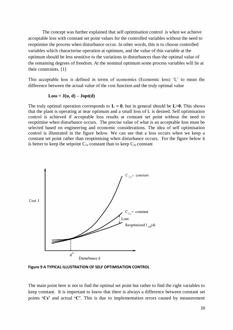
This acceptable loss is defined in terms of economics (Economic loss) „L‟ to mean the

difference between the actual value of the cost function and the truly optimal value

Loss = J(u, d) – Jopt(d)

The truly optimal operation corresponds to L = 0, but in general should be L>0. This shows

that the plant is operating at near optimum and a small loss of L is desired. Self optimisation

control is achieved if acceptable loss results at constant set point without the need to

reoptimise when disturbance occurs. The precise value of what is an acceptable loss must be

selected based on engineering and economic considerations. The idea of self optimisation

control is illustrated in the figure below. We can see that a loss occurs when we keep a

constant set point rather than reoptimising when disturbance occurs. For the figure below it

is better to keep the setpoint C1s constant than to keep C2s constant

Figure 9 A TYPICAL ILLUSTRATION OF SELF OPTIMISATION CONTROL

The main point here is not to find the optimal set point but rather to find the right variables to

keep constant. It is important to know that there is always a difference between constant set

points ‘Cs’ and actual ‘C’. This is due to implementation errors caused by measurement

21

errors and imperfect control. To minimise the effect of the errors on the operating cost, the

cost surface as a function of C should be as flat as possible. This is illustrated in figure 12

below. From this figure 11 , we were able to distinguish between three cases when it comes

to the actual implementation

Figure 11 TYPICAL STRUCTURES OF OPTIMUM BEHAVIOURS

(A) Constrained optimum; In this case the optimal cost is achieved when one of the

variables is at its maximum or minimum. There is no loss imposed by keeping the

variable constant at its active constant. Implementation of an active constraint is

usually easy, eg; is easy to keep a valve fully open or closed.

(B) Unconstrained flat optimum; in this case the cost is insensitive to the value of the

controlled variable C.

(C) Unconstrained sharp optimum; In this case the cost operation is sensitive to the actual

value of the controlled variable C and self optimising control is not possible. In this

case, we would like to find another controlled variable C in which the optimum is

flatter

According to Skogestad[1], self optimisation control is when near optimal operations can

be achieved with Cs constant, in spite of disturbances „d’ and implementation error ‘n’ (n=

C+ n). In figure 4 below, you see the interaction between the local optimisation layer and the

feedback control layer. The two layers interact through the controlled variables C, whereby

the optimiser computes their optimal set points Cs, and the control layer attempts to

implement them in practice that is to get C≈ Cs.

22

Figure 10 IMPLEMENTATION WITH SEPARATE OPTIMISATION AND CONTROL

3.5. SELECTION OF CONTROL VARIABLES:

According to Skogestad (2000), the following rules must be observed while selecting a

controlled variable „CV‟ suitable for constant set point control (Self optimisation)

• Rule 1: The optimal value for CV c should be insensitive to disturbances d

(minimizes effect of setpoint error)

• Rule 2: c should be easy to measure and control (small implementation error n)

• Rule 3: c should be sensitive to changes in u (large gain |G| from u to c) or equivalently the optimum J

opt should be flat with respect to c (minimizes effect of implementation

error n)

• Rule 4: For case of multiple CVs, the selected CVs should not be correlated.

The first rule minimises the effect of disturbances d. The second rule reduces the magnitude of n. The last two rules minimises the effect of the implementation error n. These four rules can be summarised by the following single rule; Select controlled variables C for which the controllable range is large compared to the sum of

optimal variation and control. (Skogestad and Postlethwaite, 1996) [13]. controllable range

means the range that C may reach by varying the inputs (degrees of freedom) u, the „optimal

variation‟ is the expected variation in „Copt‟ due to disturbance and the control error is the

implementation error n.

There are some quantitave methods for control variable selection and they are explained

below;

23

3.5.1. SELECTION OF CONTROL VARIABLE C BY MINIMUM SINGULAR VALUE RULE

Select controlled variables c such that we maximize the minimum singular value of the scaled

gain matrix G (from u to c ; here u ‟s are the “original” degrees of freedom). This requires

that the candidates c’s have been scaled with respect to their span. This can be represented as;

Gs = S1GJuu-1/2

( 1)

S1 = diag [1/span (ci) ] (2)

Span ci = [nic ]+ [∆ci, opt (d)] (3)

Span is the sum of optimal variation plus control error. Worst case loss is given below;

1

2

max 2 1/2 21 1

1 1

2 2( ( ))max

ce uu

L zS GJ

(4)

The full derivation of this rule is given by Halvorsen et al. (2003). Although this rule is not

exact, especially for plants with an ill-conditioned gain matrix like distillation columns,, it is

very simple and it works well for most processes (Halvorsen et al., 2003).

Maximum gain rule has some limitations like;

It may be impossible to calculate the value of Juu as a scalar times unitary matrix but

this limitation can be corrected by defining S2 = Juu-1/2

Maximum gain rule assumes that the worst case setpoint errors ∆ci,opt (d) for each

CV can appear together. In general ∆ci,opt (d) are correlated.

These limitations can lead to sub optimal set of CVs.

Hence, to overcome these limitations we use the exact local method.

3.5.2. SELECTION OF CONTROL VARIABLE C BY EXACT LOCAL METHOD

The exact local method was presented by Halvorsen et al. (2003). This method utilizes a

Taylor series expansion of the loss function, and the exact value of the worst case loss is:

1

2

max1

( ([ ]))max

2

y

c

d n

e

M ML L

(5)

Where: (6)

Md = J1/2

uu (J−1

uu Jud − G−1Gd)Wd

Mny = J

1/2uu G

−1We (7)

Md represents the loss in the primary variables caused by disturbances and Mny represents

the loss caused by implementation error. The magnitude of the disturbances and

implementation error enter into the diagonal matrices Wd and We, respectively. The steady-

24

state gains G and Gd and the second order derivatives Juu and Jud may be obtained

numerically by applying small perturbations in the inputs u.

3.5.3. SELECTION OF CONTROL VARIABLE C BY MEASUREMENT COMBINATION METHOD

Another option is to use the linear combinations of measurements

c =Hy, (8)

where; H is a linear combination rather than a selection matrix. Y is the available

measurements, including the inputs u used by the control system.

The goal of using several measurements is to further reduce the effect of disturbances and

implementation errors. For a given set of measurements (ys), the combination matrix H can

be evaluated in two different ways:

3.5.3.1 OPTIMAL METHOD:

In this method, we write the linear model in terms of the measurements y as;

y = Gyu + G

yd (9)

Locally, the optimal linear combination is obtained by minimizing σ([Md Me ]) in (2) with

We = HWny , where Wny contains the expected measurement errors associated with the

individual measured variables; see Halvorsen et al.(2003). Note that H enters (2) indirectly,

since G = HGy and Gd = HGy d depend on H. However, (2) is a nonlinear function of H and

numerical search-based methods need to be used.

3.5.3.2 NULL SPACE METHOD

According to Alstad and Skogestad (2007)[4], null space method is the simpler method for

finding H where we neglect the implementation error, i.e., Me = 0.Then, a constant set point

policy (c = r) is optimal if Copt (d) is independent of d, that is, when Copt = 0 *d in terms of

deviation variables. Note that the optimal values of the individual measurements yopt still

depend on d and we may write

yopt = Fd (10)

where F is the optimal sensitivity of y with respect to d. We would like to find c = Hy such

that Copt = Hyopt = HFd = 0 * d for all d. To satisfy this, we must require HF = 0 or that H

lies in the left null space of F. This is always possible, provided

ny ≥ nu+nd. (11)

This is because the null space of F has dimension ny = nd and to make HF = 0, we must

require that

nz = nu < ny- nd. (12)

25

This shows Md = 0 when Hf = 0. If there are too many disturbances, i.e. ny < nu+nd, then

one should select only the important disturbances (in terms of economics) or combine

disturbances with a similar effect on y (Alstad, 2007).

In the presence of implementation errors, even when HF = 0 such that Md = 0, the loss can be

large due to non-zero Me. Therefore, the null space method does not guarantee that the loss L

using a combination of measurements will be less than using the individual measurements.

One practical approach is to select first the candidate measurements y, whose sensitivity to

the implementation error is small (Alstad, 2007).

26

4.0 MODELLING AND SIMULATION OF TEALARC LNG PROCESS PLANT The following chapter describes the modelling and simulation of Tealarc LNG process plant

with major emphasis on:

Process description

Modelling of some important unit operations

Specifications made for the entire process plant.

4.1 Process description Tealarc LNG process plant is shown in figure below. It has two sections:

Pre cooling cycle

Liquefaction cycle

In this project, I tried to simulate and optimise each part of the Tealarc process plant

separately.

4.1.1PRE-COOLING CYCLE

This pre-cooling cycle primarily consists of propane and ethane gas which is cooled from a

temperature of about 86℃ to -64℃ at a five pressure level. It is also used to cool and partially

liquefy the mixed refrigerant (MR) coming from the Liquefaction cycle to a low temperature

of about -62℃. The cooling of this refrigerant is achieved by the help of the three heat

exchangers (PLNG100; PLNG101; PLNG102). In the heat exchangers, the pre-cooling gas

boils and evaporates in the shell side of the heat exchanger while the compressed and cooled

mixed refrigerant flows in the immersed tube side. There is indirect heat exchange between

the two and as a result pre cooling and cooling takes place. The centrifugal compressors

recover the evaporated pre-cooling gas stream and compress the vapour to about 2260KPa at

three pressure level. It is further condensed against water or air and recycled back to the heat

exchangers to continue the circulation.

In the mixed refrigeration cycle (MR), the compressed and pre-cooled MR from the

liquefaction cycle is partially liquefied and cooled to a temperature of about -62℃. This is

made possible by the interaction in the heat exchangers between the pre-cooling gas stream

and the MR stream. In the heat exchangers the MR is cooled, partially liquefied and reduced

to a pressure of about 2400KPa. This cooled and partially liquefied MR is flashed at constant

pressure resulting in cooled refrigerant liquid and cooled refrigerant vapour. This separated

component is recycled back to the liquefaction cycle through the second heat exchanger

where it is sub-cooled and it helps in sub-cooling the feed natural gas. This pre-cooling

process flow sheet is shown in figure 11 below:

27

Figure 11 TEALARC PRE-COOLING FLOWSHEET

4.1.2 Liquefaction cycle

The liquefaction cooling cycle consists of three heat exchangers (LNG100; LNG101,

LNG102), two compressors and a flash tank as you can see in the figure 12 below. In the

flash tank as said above the mixed refrigerant from the pre-cooling cycle is split into a vapour

and liquid fraction in other to utilise the different boiling points of the two components.

These two fractions of the mixed refrigerant stream is further cooled in the second heat

exchanger (LNG101) and then reduced in pressure and vaporized by heat exchange while

cooling the feed gas and low level mixed refrigerant.

Treated natural gas is feed into the first heat exchanger (LNG 100) where, by indirect heat

exchange between the mixed refrigerant and the natural gas stream, the temperature of the

feed natural gas is cooled from 30℃ to about -52℃ while that of the mixed refrigerant is

superheated from about -56℃ to about -4℃. This superheated mixed refrigerant is

compressed by compressors (K102 and K101) and subsequently cooled before it is

recycled back to the pre-cooling plant. The feed natural gas is further sub-cooled in the

second heat exchanger by indirect heat exchange between the recycled, cooled and

partially liquefied mixed refrigerant.

At the third heat exchanger, the sub-cooled natural gas is further cooled and liquefied at it‟s

at a temperature of -157℃, which is about the boiling point temperature of methane gas. The

pressure of the natural gas stream is further reduced to the atmospheric pressure with the help

of the expander (K101) thereby reducing the temperature to about -163℃. The liquefied

natural gas is flashed and stored in the LNG tank. The process is a continuous cycle.

28

Figure 12 TEALARC LIQUEFACTION FLOWSHEET

4.2 MODELLING AND SIMULATION OF THE UNIT OPERATIONS

Generally, when simulating a process plant like this, one must model some important units of

operations like; heat exchangers, compressors/expanders, coolers and valves. This steady

state model of the Tealarc LNG process plant was built by selecting from UNISIM library the

proper unit operation models, describing the heat and mass transfer taking place during the

process, defining the streams, characterising heat exchangers, and other plant equipment and

choosing the proper set of independent variable. SRK (Soave-Redlich-Kwong) fluid package

was used for the thermodynamics calculations in this process model. Some of these modelled

unit operations are:

4.2.1LNG Heat exchangers

LNG HEAT EXCHANGER

29

In modelling LNG Heat exchangers in UNISIM, you are expected to either specify the heat

loss or allow the heat loss calculated from specified values (overall U value or ambient

temperature). The heat transfer area (A) and minimum temperature approach are calculated

by UNISIM. The heat loss is calculated using;

Q = UA(T-Tamb)

I made sure that the pressure drop between inlet and out let streams are specified so that the

necessary degrees of freedom in the heat exchanger will be achieved (Degree of freedom =

0). UNISIM sees the number of streams around the heat exchanger as variables and the

number of parameters (temperature, pressure...) as constraints. Hence, for the heat exchanger

to solve the degrees of freedom must be zero.

During the heat exchanger modelling I encountered some problems like Temperature cross in

heat exchanger and insensitivity of heat exchanger. The problem of temperature cross means

that the calculated heating curves for the different sides in the exchanger are touching or

crossing each other at some point. I tried to solve this problem by making sure that the

difference between the flowrate of the hot and cold stream is not much.

4.2.2 Compressor

The centrifugal compressor was modelled with constant efficiency of 80%, meaning that

shaft is the variable to be manipulated rather than compressor speed. I specified the outlet

streams pressure and UNISIM calculated the compressor work Ws.

One problem I encountered during the compressor modelling is the problem of water inlet

into the compressor. In order to avoid water inlet into the compressor i made sure that the

inlet stream is superheated. Superheated streams have temperature higher than there dew

point temperature.

30

4.2.3 SW Coolers

Coolers are modelled by specifying the out let temperature and allowing UNISIM to calculate

the duty Q. I also made sure that the maximum cooling temperature (30℃) of the cooler is

specified for efficiency.

SW cooler duty Q = m (hout−hin)

4.2.4 VALVES

For the valves, there are three different sizing methods; Cv , Cg and k methods. I selected

universal gas sizing method for my model; it uses the equation below;

This universal gas sizing equation incorporates both the basic Cv and Cg equations into a

single, dual-coefficient equation where the new factor Cf is introduced. Cf is the ratio the gas

sizing coefficient and liquid sizing coefficient.

31

4.3 SPECIFICATIONS MADE FOR THE MODELLING AND SIMULATION OF THE

ENTIRE PLANT I made the following specifications while modelling the entire Teal arc LNG process plant

and I will like to point out that I simulated the two sections of the plant sequentially(one after

another). The specifications are shown in the table 4 and 5 below:

Table 3 GIVEN DATA FOR THE SIMULATION

Mixed Refrigerant composition (mol%)

Natural Gas composition( mol%)

Methane 0.45 Methane 0.897 Ethane 0.45 Ethane 0.055 Propane 0.02 Propane 0.018 n-butane 0.00 n- butane 0.001

Nitrogen 0.029

Nitrogen 0.08 Pre-cooling temp -62℃ Pre-cooling pressure 2400KPa

Natural gas feed pressure 4000KPa Natural Gas feed temperature 30℃

Table 4 SPECIFICATIONS FOR THE SIMULATION OF LIQUEFATION PLANT

Degrees of freedom for the design (11DOF)

LNG 100............................ UA=9.6e6KJ/C-h

LNG 101............................ UA1=1.92e8KJ/C-h

LNG 101............................. UA2=1.1e8KJ/C-h

LNG 101............................... UA3=1.9e8KJ/C-h

LNG 102.................................. UA1=2.0e7KJ/C-h

LNG 102.................................. UA2= 1.2e7KJ/C-h

Choke valve (VLV-101) to set stream L6 pressure to ≥365KPa

Compressor (K-102) to set stream L12 pressure to 3000KPa

Compressor (K-100)to set stream L14 pressure to 3500KPa

Cooler (E-100) for stream L13 temperature ≥ 25℃

Cooler (E-102) for stream L15 temperature =30.15℃

You will notice from this specification that the three heat exchangers (LNG100,

LNG101.LNG102) had six specifications (UA), the choke valve had one, two coolers have

two specifications and the two compressors have two specifications, making it a total of

eleven specifications for the design.

32

Table 5 SPECIFICATIONS FOR THE SIMULATION OF THE PRE-COOLING PLANT

1.Choke valve(VLV-102) to set pressure of Stream P11.......≥170KPa

2. Choke valve(VLV-101) to set pressure of stream P9..........≥ 400KPa

3. Choke valve (VLV-100) to set pressure of stream P5........ ≥800KPa

4. SW cooler (E-101) to set temperature of stream P17. =30℃

5. Compressor (K-100) to set pressure of stream P20.............. = 2260KPa

6.SW cooler (E-100) to set temperature of stream P1 =30℃

7. Molar flow rate of the split stream (P3)..... = 5.040e4kgmol/hr

8. Molar flow rate of the split stream (P7)..... = 2.262e4kgmol/hr

9.Molar flow rate of the pre cooling fluid.... = 8.733e4kgmol/hr

10.PLNG 100 UA1=3.1e7KJ/C-h

11.PLNG100 UA2=3.0e6KJ/C-h

12.PLNG101 UA1=6.3e7KJ/C-h

13.PLNG101 UA 2=2.1e7KJ/C-h

14.PLNG102 UA1=6.4e6KJ/C-h

15.PLNG102 UA2=5.1e7KJ/C-h

PLNG is used here to represent the pre-cooling heat exchanger.

It is 15 Degrees of freedom for the design

33

5.0 IMPLEMENTATION OF SELF OPTIMISING CONTROL The theory of self optimisation as explained in chapter three of this report was implemented

in optimising this process simulation. I optimised each part of the process separately and

carefully followed the stepwise procedure for self optimisation as explained in Skogestad

2004[1]. Optimisation is usually carried out at optimal operation and I ensured that the

simulated Tealarc LNG process plant was at its optimum before optimisation was carried out.

5.1Optimising the liquefaction section The liquefaction process as described above is the part of the Tealarc process where the feed

natural gas is cooled, sub-cooled and liquefied. In other to optimise the process I did the

following;

5.1.1 Define Objective function

The objective function is to maximise the NG feed flow rate (36700kgmol/h). NG federate

was taken as the objective function because we got the nominal optimal condition at low

Efficiency (=Total Compressor work/NG feed rate). This implies that efficiency is inversely

proportional to NG feed rate. Hence, this is represented in terms of cost function J;

max [ / ]u

J NOK h

ln lng g energy energyJ q v q v

Subject to

( , , ) 0

( , , ) 0

f x u d

g x u d

Where;

xnx - State vector

unu - MVs

dnd - DVs

( , , )f x u d - Process model

( , , )g x u d - Other constraints in the process

variables

qlng - Production rate of LNG [kg/h]

vlng - Unit price of LNG

qenergy - Flow of consumed energy

venergy - Unit price of energy

34

5.1.2Degrees of freedom for operation

These are the manipulating variables in the liquefaction process. There are four of them remaining

after the process design because during operation heat exchangers (UA values) are fixed and

there are no heat exchangers bypasses.

Table 6 DEGREES OF FREEDOM FOR OPERATIONS IN THE LIQUEFACTION PLANT

1) Choke valve (VLV-101) used to set stream L6 Pressure≽365KPa

2) Compressor (K-102) used to set Stream L12 Pressure ≥3000KPa

3) Compressor (K-100) used to set Stream L14 Pressure ≥3500KPa

4) NG Feed rate (36700kgmol/h)

5.1.3Constraints

Constraints are those variables that consume degrees of freedom in the operation and are

necessary that these constraints are identified and controlled in the process.

Table 7 CONSTRAINTS

1) Stream L6 pressure ≥ 365KPa

2) Stream L12 Pressure ≥3000KPa

3) Stream L14 Pressure ≥3500KPa

4) LNG Product Temperature = -157℃

5.1.4Disturbances

These are those variables that may have steady state effect on the objective function

Table 8 DISTURBANCES IN THE LIQUEFACTION PLANT

1) Natural gas feed composition

2) Natural gas feed pressure

3) Mixed refrigerant feed pressure (Stream L1)

35

5.2 Optimising the pre-cooling section For the pre-cooling section, the same steps were taken to optimise the process and they are;

5.2.1Objective function

The objective function for this part of the process is to minimise the compressor work (Ws)

and is defined in terms cost function (economics)

Min J [NOK/KWh] = Wspenergy

Subject to constraints C≤0

( , , ) 0

( , , ) 0

f x u d

g x u d

5.2.2Degrees of Freedom for Operation

Is assumed that there is no bypass in heat exchanger and heat exchanger UAs are fixed

Table 9 DEGREES OF FREEDOM FOR OPERATION IN THE PRE-COOLING PLANT

1) VLV-102 to set Stream P11....... 170KPa

2) VLV-101 to set stream P9..........= 400KPa

3) VLV-100 to set stream P5........ 800KPa

4) K-100 for stream P20...............= 2260KPa

5) Molar flow rate of the split stream(P3).....= 5.040e4kgmol/hr 6) Molar flow rate of the split stream(P7).....= 2.262e4kgmol/hr 7) Molar flow rate of the pre cooling fluid....= 8.733e4kgmol/hr

The temperatures of the SW coolers were specified to their maximum cooling

temperature (30℃), hence, they were not used in the optimisation process. So i am left

with 7 degrees of freedom for the operation.

5.2.3 Constraints

Seven constraints were obtained during the design but we are applying four constraints in

the operation since is assumed that heat exchanger value is fixed.

Table 10 CONSTRAINTS FOR THE PRECCOLING PLANT

1) Minimum temperature approach in the three heat exchangers( PLNG-100, PLNG-101, PLNG-102)= 3 constraints

2) Superheating in compressor feed streams.(P12,P14,P19) = 3 constraints

3) Temperature of stream L1 ≤ -62℃

5.2.4 Disturbances

1) Pre cooling composition

36

6.0 OPTIMISATION RESULTS AND DISCUSSIONS

6.1 Nominal optimum result for liquefaction plant

LNG flow rate is maximised with a fixed temperature of 30℃ after the SW cooler and 4

degrees of freedom for operation from the 11 degrees of freedom for design. The following

results were obtained at optimum solution;

Table 11 NOMINAL OPTIMUM RESULT FOR LIQUEFATION PLANT

Obj. Function (Kgmol/h)

NG exit Temp (℃)

PL6 (KPa)

PL12 (KPa)

PL14(KPa) Compressor work K-102(KJ/h)

Compressor work K-100(KJ/h)

36700 -157 365 3000 3500 5.451e8 2.573e7

6.2 ACTIVE CONSTRAINTS

Active constraints are those inequalities that turned to equalities at optimal solution. Most of

the degrees of freedom are used to satisfy active constraints.[1]

After optimising the liquefaction process cycle, the following were found to be active

constraints;

1. Pressure of stream L12 = 3000KPa

2. Pressure of stream L14 = 3500KPa

3. Pressure of stream L6 = 365KPa

4. Temperature of NG after cooling = -157℃

Hence, you can see from this result that there is no unconstraint degree of freedom, since all

the available degrees of freedom are used to satisfy the active constraints. Natural gas feed

rate was used to set the LNG product temperature at-157℃

37

6.3 Optimal Result with Disturbance I considered the 3 disturbance variables in table 8 above, the disturbances were used in both

maximum and minimum value. The result is shown below: bold face shows the result at the

maximum disturbance value.

Table 12 OPTIMUM RESULT WITH DISTURBANCES

Optimisation Result Table at Nominal Optimal condition with disturbance d1(NG feed pressure at 3990KPa and 4010KPa).

Obj.Funct. (Kgmol/h)

NG exit Temp (℃

PL6 (KPa)

PL12 (KPa)

PL14(KPa)

Compressor work K-102(KJ/h)

Compressor work K-100(KPa)

Total compressor work(KJ/h

36636.7 -157 365 2999.83

3499.85 5.451e8 2.573e7 5.7083e8

36814.7 -157. 365 2999.83

34999.85 5.442e8 2.573e7 5.6993e8

Optimisation Result Table at Nominal Optimal condition with disturbance d2 (NG feed composition: CH4=0.89, C2=0.05, C3= 0.028, n-C4=0.002, N2=0.029, CH4=0.9, C2=0.052, C3= 0.018, n-C4=0.001, N2=0.030)

Obj. Funct (Kgmol/h)

NG exit Temp (℃

PL6 (KPa)

PL12 (KPa)

PL14 (KPa)

Compressor work K-102(KJ/h)

Compressor work K-100(KJ/h)

Total compressor work(KJ/h

36632.6 -157 365 2999.83 34999.85 5.432e8 2.573e7 5.6893e8

36894.2 -157 365 2999.83 34999.85 5.465e8 2.573e7 5.7223e8

Bold face is the maximum value for the disturbance

Optimisation Result Table at Nominal Optimal condition with disturbance d3 (Mixed Refrigerant Pressure 2390KPa and 2410KPa)

Obj. Funct (Kgmol/h)

NG exit Temp (℃

PL6 (KPa)

PL12 (KPa)

PL14 (KPa)

Compressor work K-102(KJ/h)

Compressor work K-100(KJ/h)

Total compressor work(KJ/h

36700 -157 365 2999.83

34999.85

5.451e8 2.573e7 5.7083e8

36843 -157 365 2999.83

34999.85

5.460e8 2.573e7 5.7173e8

Bold face is the maximum disturbance value

38

6.3 Optimisation result for the pre cooling part I was able to do only one optimisation simulation for the pre-cooling part because of time

constraints. The result is shown on the table below:

Table 13 OPTIMUM RESULT FOR THE PRE-COOLING PLANT

Obj.fuct(kJ/h) Molar flow

P3(kgmol/h)

Molar flow

P7(kgmol/h)

Molar

flow1(kgmol/h)

P5(KPa) P9(KPa) P11(KPa) P20(KPa)

38.63e8 5.040e4 2.400e4 8.800e4 808 400 170 2260

6.3.1 Active constraint

Stream L1 (℃) = -61.91 was seen to be active at optimum solution.

6.4 DISCUSSION OF RESULTS

It can be seen from the optimisation result table with disturbance that the production rate was

still maximised despite the influence of the disturbance variables during operation. Changing

the operating parameters such as inlet gas pressure, and gas composition (particularly

nitrogen content) has a big influence on plant performance. Decrease in the inlet natural gas

pressure causes the decrease of Joule-Thompson effect.[8]

LNG production rate increased with increase in pressure of the NG feed and decreased with

decrease in pressure of the NG feed. This is confirmed in the work done by Jørgen [16]

Increase in the mixed refrigerant pressure caused a subsequent increase in the LNG

production rate. This is caused by the heat exchange that takes place inside the heat

exchanger between the pre cooled mixed refrigeration gas and the feed natural gas.[2]

The main energy loss of a natural gas liquefaction process exists in compressors and heat

exchangers. In this paper, the matching of the heating and cooling curves between the feed

gas and the mixed-refrigerant in heat exchangers was analyzed. The temperature difference

and heat exchange load in heat transfer contribute to the energy loss, so large temperature

difference and heat exchange load are the primary reasons of the energy loss in heat

exchangers [18,19]. Sure the heat flow is not the only one affected by the changing

temperature; the enthalpy and pressure also are the ones. The matching of the heating and

cooling curves in heat exchangers in the liquefaction Processes was analyzed. It can be seen

from the results shown in figure 14 and figure 15 below that heat loss is minimised in the heat

exchangers at optimum solution. The minimum temperature approach for the three heat

exchangers in both the liquefaction and pre-cooling plant (LNG100 <5℃, LNG101and

LNG102<2℃), corresponds to the same value explained in [18] as the minimum temperature

approach for high efficient cryogenic heat exchangers.

39

Figure 13 TEMPERATURE(C)- HEAT FLOW(KJ/h) FOR LIQUEFACTION PLANT.

Figure 14 TEMPERATURE(C)- HEAT FLOW(KJ/H) FOR PRECOOLING PLANT

40

7.0 Conclusion This project report on simulation, optimal operation and self optimisation of LNG process

plant has shown the systematic implementation of Control structure/ Plant wide control to

natural gas liquefaction industry. To obtain optimal solution, steady state simulation of the

Tealarc LNG process plant was carried out by the help of UNISIM simulator. I simulated and

optimised the pre-cooling and liquefaction part of the plant separately using the model

specifications shown in table 4 and 5 in this report.

The simulated process was optimised using the plant wide control method by skogestad [1].

The optimal result in table 12 and 13 shows that the defined objectives function (cost

function) for the liquefaction process was achieved subject to certain constraints and degrees

of freedom. We also found out that all the degrees of freedom for operation were used to

satisfy the active constraints during operation. Hence, self optimisation control could not be

carried out because you need at least one unconstrained degree of freedom to perform self

optimisation control.[1]

Heating curve of the heat exchangers for the pre-cooling and liquefaction plant (figure 15 and

16) shows reduced energy loss in the heat exchangers which is basically one major objective

function that must be minimised in natural gas liquefaction process.[18]

41

8.0REFERENCES [1] Skogestad, S., Control structure design for complete chemical plants.Computers &

Chemical Engineering, 2004. 28(1-2): p. 219-234.

[2] Paradowski, H. and J.-P. Dufresne, Process analysis shows how to save energy.

Hydrocarbon Processing, July, 1983: p. 103-108.

[3] Halvorsen, I.J., et al., Optimal selection of controlled variables. Ind.Eng.Chem.Res, 2003.

24(14): p. 3273-3284.

[4] Alstad, V. and S. Skogestad, Null Space Method for Selecting Optimal Measurement

Combinations as Controlled Variables. Ind. Eng. Chem. Res., 2007. 46: p. 846-853.

[5] LNG Remains Keystone to Development of Qatari Gas Resources, LNG Express, Vol.15,

No. 1., Jan 2005

[6].Kennett, A., Limb, D., Czarnecki, C.: “Offshore Liquefaction of Associated Gas- a

suitable process for the North Sea”, Offshore Technology Conference, May, 1981.

[7] “Natural Gas”, / International Energy Outlook, Energy Information Administration,

Office of Integrated Analysis and Forecasting, U.S. Department of Energy, Washington, DC,

March 2002

[8] Finn A.J., Johnson G.L., Tomlinson T.R., „Developments in natural gas liquefaction”, Hydrocarbon Processing April 1999, 47-59

[9].Sandler, S., 2006, “Chemical, Biochemical, and Engineering Thermodynamics”, Wiley,

fourth edition, United States of America.

[10] Perry, R.H. and Green, D.W. (1984). Perry's Chemical Engineers' Handbook (6th

Edition ed.). McGraw Hill, Inc.. ISBN ISBN 0-07-049479-7. (see pages 12-27 thro12-38)

[11]Edgar, T.F., and Himmelblau, D.M., 1988, “Optimization of chemical process”,

McGraw-Hill, United States of America.

[12] Nocedal, J., and Wright, S., 1999, “Numerical optimization”, Springer series in

operation research, United States of America

[13] S. Skogestad, I. Postlethwaite, Multivariable Feedback Control, John Wiley & Sons,

New York, 1996.

[14] Linnhoff March, „Introduction to pinch technology”, 1998

[15] “Refrigeration cycle using a mixed refrigerant”, International Patent Application,

PCT/GB98/01720

[16] Jensen, Jørgen B., Skogestad, S.: Optimal operation of a simple LNG process, Adchem

2008

[17] Unisim Design user Guide, Honey well, March 2008, R380 Release.

42

[18] Seider WD, Seader JD, Lewin DR. Process design principles. New York: Wiley; 1998.

p. 207–42.

[19] Liu LY, Daugherty TL, Brofenbrenner JC. LNG liquefier efficiency. In: Proceedings of

the LNG 12, Institute of Gas Technology, Perth, 1998

43

APPENDIX -A A TYPICAL TEMPERATURE-ENTHALPY CURVE

Figure 15 A TYPICAL TEMPERATURE ENTHALPY CURVE [SOURCE:15]

44

APPENDIX-B WORKBOOK OF ALL STREAMS AND PROPERTIES FOR BOTH

LIQUEFACTION AND PRE-COOLING

45

46

47

48