Embed Size (px)
Citation preview
Simulation of Thermo-mechanical Deformation in High Speed Rolling of Long Steel Products
A Thesis
Submitted to the Faculty
of the
WORCESTER POLYTECHNIC INSTITUTE
In Partial Fulfillment of the Requirements for the
Degree of Master of Science
in
Mechanical Engineering
by
__________________
Souvik Biswas
September 11, 2003
Approved by:
______________________________
Prof. Joseph. J. Rencis
Advisor
______________________________
Dr. Bruce V. Kiefer
Industrial Advisor
______________________________
Prof. Zhikun Hou
Graduate Committee Representative
______________________________
Mr. Horacio Gutierrez
Industrial Advisor
______________________________
Prof. Satya S. Shivkumar
Member, Thesis Committee
______________________________
Prof. Richard D. Sisson, Jr.
Member, Thesis Committee

i
Abstract
The goal of this thesis is to develop an off-line process model that can be used by engineers to expedite the optimum selection of process parameters in a high-speed mill for hot rolling of long steel products in the United States (U.S.) steel industry. The software tool developed in this work will better enable steel mill manufacturers and operators to predict the geometric properties of the hot rolled material. The properties predicted by the model can be used by the manufacturer to determine if customer requirements for the final rolled product can be met with the specified equipment and rolling conditions. This model can be used to reduce manufacturing costs and shorten production cycle time while assuring product quality.
A coupled thermo-mechanical simulation model was developed using the commercial finite element code ABAQUS. The rolling model is three-dimensional, thermo-mechanical, transient and nonlinear. Two case studies are considered to demonstrate how the finite element model predicts geometric parameters which are necessary to satisfy customer requirements. The finite element model was validated through full-scale testing and verified with existing theoretical/empirical models. The results of the test cases demonstrate that the finite element model is able to predict geometrical properties to ensure that the steel mill satisfies the customer requirements.
A Java pre- and post-processing graphical user-oriented interface has been developed to aid a mill engineer with little or no finite element experience throughout the analysis process of the finishing rolling stands. The Java program uses the finite element analysis results to predict roundness and tolerance customer requirements. Other parameters that are determined include spread, cross-sectional area, percentage reduction in area, incremental plastic strain and total plastic strain and roll force.

ii
Acknowledgement
I would like to express my gratitude to Prof Joseph J. Rencis, my advisor for helping guiding and encouraging me to complete this thesis. I also thank Dr. Bruce Kiefer and Mr. Horacio Gutierrez of Morgan Construction Company for providing me with technical knowledge, giving valuable advice during the course of this project and clearing my doubts whenever necessary. I would like to thank Prof. Hou, Prof. Shivkumar and Prof. Richard Sisson for being members of my thesis committee. I also thank Mr. Sia Najafi, Computer Manager, ME Department, WPI for helping me in whenever I faced any difficulty. I would also like to thank the program secretary, Ms. Barbara Edilberti for helping me out during my stay at WPI. I would like to thank my family for supporting me throughout, during my study in WPI. I would also like to thank my friends for helping me out during my study in WPI.

iii
Table of Contents Section PageAbstract i Acknowledgement ii Table of Contents iii List of Figures vi List of Tables viii List of Symbols x 1. Introduction 1 1.1. Necessity for Off-line Rolling Simulations in the U.S. Steel Industry 1 1.2. What is Missing in Deformation and Microstructure Rolling Simulations? 2 1.3. Significance of this Work 2 1.4. Goal And Objectives 3 2. The Finishing Rolling Process and Model 4 2.1. Processing Stages in a Rolling Mill 4 2.2. Importance of the Finishing Rolling Stage 5 2.3. Requirements of an Offline Rolling Model 6 2.4. Challenges in Developing an Off-line Rolling Model 7 2.5. Rod and Bar Rolling Simulation Codes used by the Overseas Steel Industry 9 3. Theoretical and Empirical Geometric and Deformation Models for Steel Rod and Bar Round-Oval, Oval-Round Pass Rolling 12
3.1. Overview 12 3.2. Spread and Cross-sectional Area 12 3.3. Mean Effective Plastic Strain 17 3.4. Roll Force 22 4. Predicting Flow Stress Behavior of Steel at High Temperature and Strain Rates 25 4.1. Overview 25 4.2. Experimental Studies 25 4.3. Empirical Constitutive Equations 27 5. Case Studies and Discussion 30 5.1. Overview 30 5.2. Case Study #1- Republic Engineered Products, Finishing Stands 31 5.2.1. Product Manufactured in the Mill 31 5.2.2. Configuration of the Rolling Stands 31 5.2.3. How is the Problem Modeled using FEM? 33 5.2.4. Comparison of Finite Element Results with Full-scale Testing and Theoretical Calculation 36
5.2.5. Are Customer Requirements Satisfied? 48 5.3. Case Study #2 - POSCO No. 3 Mill Roughing Stands 49 5.3.1. Product Manufactured in the Mill 49 5.3.2. Configuration of the Rolling Stands 49
iv
5.3.3. How is the Problem Modeled using FEM? 50 5.3.4. Comparison of Finite Element Results with Theoretical Calculation 53 6. Conclusion 64 7. Future Work 65 7.1. Theoretical Thermo-Mechanical Model 65 7.1.1. Theoretical Calculation of Stock Temperature during the Rolling Process 65 7.1.2. Microstructure Evolution of Stock During the Rolling Process 66 7.2. Finite Element Modeling 67 7.2.1. Calculation of Output Parameters for Rolling Mill by post processing FEM Output Results 67
7.2.2. Improvements to the Finite Element Model 67 7.3. Improvement of Theoretical-Empirical Model Based on Numerical Experiments 67 References 69 Appendix A: Pre-processing Finish Rolling Stage GUI for ABAQUS 77 A.1. Introduction 77 A.2. Programming Environment 77 A.3. Steps of Rolling Simulation Analysis 78 A.4. Pre-processor GUI Screen Layout 78 A.4.1. GUI Layout 78 A.4.2. Input Modules 78 A.4.2.1. Roll & Groove Geometry Module 79 A.4.2.2. Roll Properties 82 A.4.2.3. Roll Boundary Conditions 83 A.4.2.4. Feed Section Geometry 84 A.4.2.5. Stock Properties 86 A.4.2.6. Stock Initial Conditions 87 A.4.2.7. Stock Meshing Module 88 A.4.2.8. Contact Information 88 Appendix B: Post-processing Finite Element Simulation Results 90 B.1. Introduction 90 B.2. Steps of Rolling Post-Processing 90 B.2.1. Python Script Program 91 B.2.2 Java Post-processing Program 91 B.2.2.1. Spread Calculation 91 B.2.2.2. Cross Sectional Area Calculation 91 B.2.2.3. Total Plastic Strain Calculation 92 B.2.2.4. Incremental Plastic Strain Calculation 92 B.2.2.5. Roll Force Calculation 92 B.3. Java Post-processor GUI Screen Layout 93 B.3.1. GUI Layout 93 B.3.2. Post-processor Module 93
v
Appendix C: Initial Finite Element Mesh 94 C.1. Overview 94 C.2. Rod and Bar Geometry 94 C.3. Constructing a Symmetrical Mesh in ABAQUS 95 C.4. Element Distortion Metric Guidelines 95 C.5. Element Size 96 Appendix D: Full Scale Mill Testing 97 Appendix E: Important Aspects of the Finite Element Model 100 Appendix F: Additional Finite Element Analyses 103 F.1. Results of Finite Element Solution for the RSM Case (Section 5.2) 103 F.2. Results of Finite Element solution for the POSCO case (Section 5.3) 111 Appendix G: Mesh Convergence Study 115 G.1. Convergence Study for Spread and Area for Last Pass of Republic Engineering Products, Lorain, OH RSM Mill 115
Appendix H: A New Approach for Theoretical Calculation of Stock Surface Profile in Multi-Stand Rolling 117
H.1. Overview 117 H.2. Proposed Approach 117 H.3. Advantages and Disadvantages 118 Appendix I: Conference Paper 119 Appendix J: Thesis presentation 133

vi
List of Figures
Figure 2.1. Rod mill with a four stand finishing block. 5 Figure 2.2. Proposed off-line finishing rolling process rod and bar simulation model. The
shaded part of this proposed model is only considered. 8
Figure 2.3. Coupling scheme for macroscopic and microscopic models. 9 Figure 3.1. Spread and side free surface. 13 Figure 3.2. Illustration of equivalent rectangle method in round-oval pass for calculation of
equivalent height of incoming stock and roll groove. 15
Figure 3.3. Schematic representation of parallelepiped deformation of equivalent rectangle section (reprinted from Lee et al. [3.11]).
19
Figure 3.4. Three methods of computing an equivalent cross sectional area for the oval round stand. (a) Method of width-height ratio (b) Method of maximum height (c) Method of maximum width (reprinted from Lee et al. [3.11]).
20
Figure 5.1. Finishing stands of Republic Engineered Products, RSM Mill 33 Figure 5.2. Arrangement of ABAQUS/Explicit rolling stands in Republic Engineered
Products RSM mill. 35
Figure 5.3. Comparison of finite element and theoretical solutions for finishing Stand #1. 39 Figure 5.4. Comparison of finite element and theoretical solutions for finishing Stand #2. 41 Figure 5.5. Comparison of finite element and theoretical solutions for finishing Stand #3. 43 Figure 5.6. Comparison of finite element and theoretical solutions for finishing Stand #4. 45 Figure 5.7. Finite element solution of total plastic strain (mm/mm) variation in stock at each
stand. 47
Figure 5.8. Roughing stands POSCO No. 3 mill. 50 Figure 5.9. Arrangement of ABAQUS/Explicit rolling stands in POSCO No. 3 mill. 52 Figure 5.10. Comparison of finite element and theoretical solutions for Roughing Stand #1. 55 Figure 5.11. Comparison of finite element and theoretical solutions for Roughing Stand #2. 57 Figure 5.12. Comparison of finite element and theoretical solutions for Roughing Stand #3. 59 Figure 5.13. Comparison of finite element and theoretical solutions for Roughing Stand #4. 61 Figure 5.14. Finite element solution of total plastic strain (mm/mm) in stock. 63 Figure 7.1. Proposed flowchart if steady-state finite element modeling is successful. 68 Figure A.1. Flowchart for GUI software. 78 Figure A.2. Finish groove. 79 Figure A.3. Oval groove. 80 Figure A.4. Screen layout of the groove geometry module. 82 Figure A.5. Screen capture of the Material data module. 83 Figure A.6. Screen layout for entering plastic strain curve. 83 Figure A.7. Screen layout for entering stock geometry data. 84 Figure A.8. Screen layout for specifying the file, which contains stock geometry data for
stock geometry module. 85
Figure A.9. Screen layout for entering boundary conditions data. 86 Figure A.10. Screen layout for entering initial conditions data. 86 Figure A.10. Screen layout stock initial conditions Module. 87 Figure A.12. Screen layout stock meshing Module. 88

vii
Figure A.13. Screen layout Roll/Stock Contact Information Module. 89 Figure B.1. Flowchart for Java post-processing software. 90 Figure B.2. Screen layout Post-processor Module. 93 Figure C.1. Planes of symmetry in a typical rod/bar. 94 Figure C.2. Symmetrical mesh in rod/bar. 95 Figure G.1. % Error of Finite Element Results with Full-scale Mill Testing at Last Stand of
Republic Engineered Products, RSM Mill for 3 different meshes. 116
Figure G.2. Tolerance and Roundness of Finite Element Results at Last Stand of Republic Engineered Products, RSM Mill for three different meshes.
116
Figure H.1. Roll Groove surface and Stock Side Free Surface. 117

viii
List of Tables Table 2.1. Major parameters in the three stages of mill processing [2.1]. 4 Table 2.3. Comparison of overseas rod and bar rolling simulation codes. 11 Table 3.1. Models for determining spread and side free surface. 16 Table 3.2. Models for determining mean effective plastic strain. 21 Table 3.3. Models for determining roll force. 24 Table 4.1. Experimental studies for determining flow stress of steel for different
temperature, strain and strain rate ranges. 26
Table 4.2 Constitutive equations for determining flow stress of steel for different strain rates and temperatures. 29
Table 5.1. Details of Republic Engineered Products Rod Outlet and POSCO No. 3 mill. 30 Table 5.2. Details of Republic Engineered Products, Finishing rolling stands and incoming
stock. 31
Table 5.3. Details of ABAQUS/Explicit finite element model for the Republic Engineered Products, Finishing rolling stands and incoming stock. 34
Table 5.4. Comparison of full-scale mill testing, FEM and theoretical geometric results at each finishing stand for Republic Engineered Products RSM mill. 36
Table 5.5. Results after finishing Stand #1 of the Republic Engineered Products RSM mill. 40 Table 5.6. Results after finishing Stand #2 of the Republic Engineered Products RSM mill. 42 Table 5.7. Results after finishing Stand #3 of the Republic Engineered Products RSM mill. 44 Table 5.8. Results after finishing Stand #4 of the Republic Engineered Products RSM mill. 46 Table 5.9. Comparison of full-scale mill testing, FEM and theoretical geometric results at
exit of fourth finishing stand in Republic Engineered Products, Lorain, OH. 48
Table 5.10. Geometry customer requirements and a comparison with full-scale mill testing, FEM and theoretical model. 48
Table 5.11. Details of initial four roughing stands of POSCO No. 3 mill. 49 Table 5.12. Details of ABAQUS/Explicit finite element model for the POSCO No. 3 mill
roughing stands. 51
Table 5.13. Comparison of full-scale mill testing, FEM and theoretical geometric results at each roughing stand for POSCO No. 3 mill. 53
Table 5.14. Results after roughing Stand #1 of the POSCO No. 3 mill. 56 Table 5.15. Results after roughing Stand #2 of the POSCO No. 3 mill. 58 Table 5.16. Results after roughing Stand #3 of the POSCO No. 3 mill. 60 Table 5.17. Results after roughing Stand #4 of the POSCO No. 3 mill. 62 Table B.1. Information written by the python script program in the ASCII files. 91 Table C.1. ABAQUS guidelines for three-dimensional element distortion metrics. 96 Table D.1. Dimension measurements of stock samples from RSM Full-scale mill Testing 97 Table F.1. Results for Republic Engineered Products RSM mill using Lagrangian
formulation, Modified Shida [F.1] constitutive law and coarse mesh. 104
Table F.2. Results for Republic Engineered Products RSM mill using Lagrangian formulation, Modified Shida [F.1] constitutive law and medium mesh. 105
Table F.3. Results for Republic Engineered Products RSM mill using Lagrangian formulation, Shida [F.2] constitutive law and coarse mesh. 106

ix
Table F.4. Results for Republic Engineered Products RSM mill using Lagrangian formulation, Shida [F.2] constitutive law and medium mesh. 107
Table F.5. Results for Republic Engineered Products RSM mill using Lagrangian formulation, Shida [F.2] constitutive law and fine mesh. 108
Table F.6. Results for Republic Engineered Products RSM mill using ALE formulation, Modified Shida [F.1] constitutive law and fine mesh. 109
Table F.7. Results for Republic Engineered Products RSM mill using ALE formulation, Shida [F.2] constitutive law and fine mesh. 110
Table F.8. Results for POSCO No.3 mill using Lagrangian formulation, Suzuki [F.3] constitutive law and medium mesh. 112
Table F.9. Results for POSCO No.3 mill using Lagrangian formulation, Shida [F.2] constitutive law and medium mesh. 113
Table F.10. Results for POSCO No.3 mill using Lagrangian formulation, Suzuki [F.3] constitutive law and medium mesh. 114

x
List of Symbols
( )T t Stock Temperature h Heat Transfer co-efficient
rσ Stefan-Boltzmann Constant α Thermal Diffusivity dTdt
Rate of Temperature Change During Rolling
pddtε
Plastic Strain Rate
µ Co-efficient of Friction 0D Initial Grain Size
0.5t Time to complete 50% Re-crystallization ( )3T A Temperature of Alpha Dissolution
( )1T A Eutectoid Temperature fα Volume Fraction of Ferrite
carbidef Volume Fraction of Iron Carbide fγ Volume Fraction of Austenite
heatingT Temperature of Reheating
coolingT Temperature of Cooling
cooling
dTdt
Rate of Temperature Change During Cooling Process
maxW Maximum Spread of Stock at a Stand
iW Maximum Width of Incoming Stock γ Spread Coefficient
cB Interval of two Cross Points Perpendicular to the Roll Axis direction when the Stock Cross-section and Roll-Groove overlap
hA Area fraction of Stock above Roll-Groove when the Cross-section of the Stock and Roll-Groove are overlapped
sA Area fraction of Stock cut out by Bc at the inside Roll-Groove when the Cross-section of the Stock and Roll-Groove overlap
0A Cross-sectional Area of Incoming Stock
meanR Mean Radius of Roll
iH Equivalent Height of Incoming Stock
oH Equivalent Height of Outgoing Stock
ih Maximum Equivalent Height of Incoming Stock
pε Mean effective Plastic Strain

xi
iH Equivalent Height of Incoming Stock
oH Equivalent Height of Outgoing Stock
iW Equivalent Width of Incoming Stock
oW Equivalent Width of Outgoing Stock
1ε Plastic Strain in Principal Strain Direction 1
2ε Plastic Strain in Principal Strain Direction 2 F Roll Force P Average Roll Pressure
dA Total Contact Area
xC Distance where the Roll Groove and the Deformed Stock are Separated
maxL Maximum Contact Length
mK Average Resistance µ Coulomb Friction Co-efficient L Average Contact Length
mh Effective Mean Height of Stock ε Plastic Strain ε Plastic Strain Rate T Temperature of the Material (o K) t Non-dimensional Temperature of the Material C Percentage Carbon Content
Mn Percentage Manganese Content V Percentage Vanadium Content Mo Percentage Molybdenum Content Ni Percentage Nickel Content k Conductivity of Stock q Heat Generation Rate in Stock ρ Stock Density
pC Specific Heat of Stock χ Fraction of Plastic Deformation Work converted in to Heat in Stock
β Mechanical Equivalent of Heat ( )*h t Convective Coefficient between Roll and Stock *r Radius below which Heat Transfer is neglected rT Temperature at the surface of the Stock Tε Total Plastic Strain at a Stand iε Total Plastic Strain at ith Element iV Volume of the ith Element iε∆ Incremental Plastic Strain at a Stand
ε∆ Incremental Plastic Strain ith Element iijε∆ Incremental Strain Components
( )f y Groove Surface

xii
( )g y Side Free Surface

1
1. Introduction 1.1. Necessity for Off-line Rolling Simulations in the U.S. Steel Industry
Steel is still a dominant structural material in use today and will be in the foreseeable future. The U.S. steel industry has faced fierce competition from the global market for the past twenty-five years. The steel industry today is vital to both economic competitiveness and national security, employing 170,000 Americans in well-paying jobs (50% above the average for all manufacturing) [1.1]. Asia and Eastern Europe have been taking advantage of their low cost to manufacture inexpensive steel and export it at a low price [1.2]. The tendency towards producing - in a consistent manner - the finished products with specifically controlled microstructural and mechanical properties within narrow limits has distinctly intensified while the quality and dimension range have significantly increased in recent years. Furthermore, mill customers, e.g., automotive manufacturers who use the rod and bar stock to produce fasteners, valve springs and other parts, demand even narrower finished-product tolerances. For the U.S. steel industry to be globally competitive in cost and quality, it must be a leader in innovation and technology.
It is estimated that the rolling process is used in 80-90% of the steel production worldwide. However, there are currently no off-line tools commercially available in the U.S. to predict a priori the microstructure and hence, the mechanical and geometric properties, of a rolled product after the steel has been subjected to the series of operations necessary for obtaining the desired shape. Consequently, attempts to correlate the rolling characteristics with mechanical properties and microstructure in the finished product have been predominantly empirical in nature. These empirical models may at best be valid under conditions that were used to generate the data, i.e. specific mill conditions and/or type of steel, but do not provide a detailed description of parameters throughout the product. Furthermore, the rolling trials required for empirical studies are very expensive and a process model that can correlate the rolling characteristics with the microstructural parameters could be very beneficial.
During the last five to ten years, there has been a continued effort in the development of software tools by overseas mill builders, steel manufacturers and universities. These tools are increasingly being applied to the development of process improvements – to the point where some of these foreign steel producers have even made products that have a quality or property advantage over US-made products. In the case of the foreign mill builders and steel producers, who are very large companies with extensive resources, the software tools are being used to demonstrate their product’s superior performance over the US-built mills, giving them a definite competitive advantage.
This work will focus on developing a off-line software tool intended to significantly improve the process and product development of rolled steel bars and rods. As stated in [1.1], "the prediction accuracy of current deformation models (for rolling,

2
extrusion, etc.) on quantitative microstructure-property relationships is limited and is a barrier to major advances in rolling process technology." As stated above, the competitiveness of the U.S. steel industry is declining steadily. In order to reverse this trend, it is imperative that new tools be developed to aid U.S. steel makers in a global market. 1.2. What is missing in Deformation and Microstructure Rolling Simulations?
Rod and bar customers today are demanding tighter specifications for tolerances
on geometric, mechanical and microstructure properties to satisfy the requirements of the products they manufacture. These downstream users are setting requirements on those properties for products to be used in specialized applications, e.g., bridge cable, tire cords, high strength fasteners, etc. This presents a problem for many U.S. rolling mill operators, who are accustomed to meeting stringent requirements on geometric and mechanical properties but not microstructural parameters. In order to determine precise mechanical equipment and processing necessary for optimizing the microstructure, more sophisticated computer models of deformation and microstructure evolution are needed.
The coupling of the rolling process simulation with both deformation and
microstructure evolution is a capability that is missing in the U.S. steel industry - as cited by a Steel Roundtable held in 1998 by the American Iron and Steel Institute (AISI) [1.1]. A user-friendly software tool that can be used by process engineers off-line is needed for accurately predicting geometry and such microstructural characteristics as primary and re-crystallized grain size and secondary phase distribution and morphology. Furthermore, mechanical properties such as tensile strength, % reduction of area and hardness need to be correlated with microstructural parameters.
By having a more complete understanding of the rolling process, the U.S. steel
industry will be able to move ahead on improving process and product development of bar and rod products in the world market. A coupled deformation and microstructural rolling simulation tool will allow off-line analyses of "what if" studies of manufacturing options and alternative material microstructures. The tool will accelerate development cycles for new products and reduce the number of costly mill trials – totally eliminating the need for them eventually. The simulations would be used to evaluate roller groove geometries, roll gap settings, stand spacing and other parameters for design comparisons. The intelligent design of groove profiles and other process parameters is a key factor for effective processing (to get proper dimensions, internal deformation and microstructure distribution) and ensuring that the required as-rolled product properties are achieved according to customer specifications.
1.3. Significance of this Work
The significance of this work is that product development testing can be carried
out off-line via simulations yielding a major reduction in the product development cycle time and expensive on-line testing. Off-line testing can also be carried out even though full-scale facilities do not exist. As basic research, it will provide opportunities for the refinement and validation of current process models of hot rolling steel. The model will facilitate practicing engineers to use advanced technology currently unavailable to U.S.
3
companies and also provide opportunities for professional development in a field where little is currently offered in the U.S. The results of the work will also have future expansion possibilities, including the extension of the capabilities to on-line models to aid in process setup and control in the rolling mill. This work will have a broad impact on the U.S. steel industry by providing state-of-practice technology to carry out process and product development that will lead to more competitive products in U.S. and overseas markets.
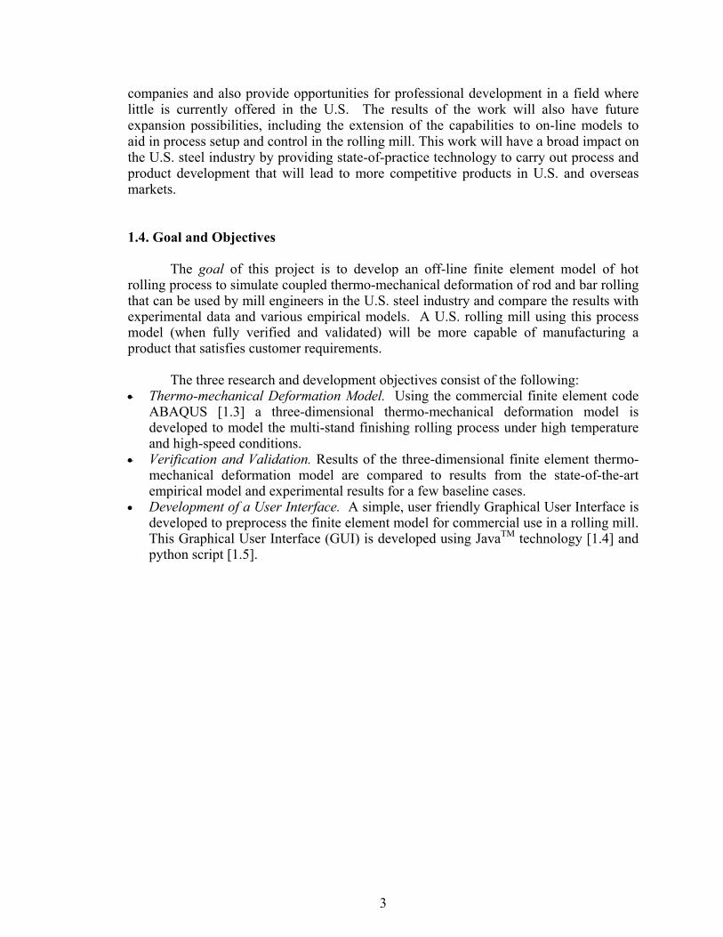
1.4. Goal and Objectives The goal of this project is to develop an off-line finite element model of hot
rolling process to simulate coupled thermo-mechanical deformation of rod and bar rolling that can be used by mill engineers in the U.S. steel industry and compare the results with experimental data and various empirical models. A U.S. rolling mill using this process model (when fully verified and validated) will be more capable of manufacturing a product that satisfies customer requirements.
The three research and development objectives consist of the following:
• Thermo-mechanical Deformation Model. Using the commercial finite element code ABAQUS [1.3] a three-dimensional thermo-mechanical deformation model is developed to model the multi-stand finishing rolling process under high temperature and high-speed conditions.
• Verification and Validation. Results of the three-dimensional finite element thermo-mechanical deformation model are compared to results from the state-of-the-art empirical model and experimental results for a few baseline cases.
• Development of a User Interface. A simple, user friendly Graphical User Interface is developed to preprocess the finite element model for commercial use in a rolling mill. This Graphical User Interface (GUI) is developed using JavaTM technology [1.4] and python script [1.5].

4
2. The Finishing Rolling Process and Model
2.1. Processing Stages in a Rolling Mill Rod and bar steel mills are comprised of equipment for reheating, rolling and
cooling as shown in Table 2.1. The primary objectives of the rolling stage are to reduce the cross section of the incoming stock and to produce the customer required section profile, mechanical properties and microstructure in the product.
Table 2.1. Major parameters in the three stages of mill processing [2.1].
ROLLING REHEATING Roughing Intermediate Finishing
COOLING
Reheating Rate Reheating Time
Reheating Temperature
Temperature % Area Reduction
Interpass Time Strain Rate
Start Temperature Cooling Rate
Final Temperature
When manufacturing long products, it is common to use a series of rolling stands
in tandem to obtain high production rates. The stands are grouped into roughing, intermediate and finishing stages (Table 2.1) - usually 26 to 30 stands. Typical temperature, speed, inter-stand time (time between each stand), true strain and strain rate ranges at each stage are shown in Table 2.2. Since cross-sectional area is reduced progressively at each set of rolls, the stock moves at different speeds at each stage of the mill. A rod rolling mill, for example, gradually reduces the cross-sectional area of a starting billet (e.g., 160 mm square, 10-12 meters long) down to a finished rod (as small as 5.0 mm in diameter, 1.93 km long) at high finishing speeds (up to 120 m/s). Typical rod mills with a four stand finishing block with stands positioned closely together and oriented in a 90o configuration to allow no-twist rolling is shown in Figure 2.1. A vast majority of the finishing blocks employ an oval-round pass sequence since it produces a good quality surface free of laps and a fairly uniform deformation across the width.
Table 2.2. Typical temperature, speed, interpass time, strain and strain rate ranges
at rolling stages.
ROUGHING INTERMEDIATE FINISHING Temperature Range 1000-1100 oC 950-1050 oC 850-950 oC
Speed Range 0.1-1 m/s 1-10 m/s 10-120 m/s Inter-Stand Time
Range 10300 - 1600 ms 1300 – 1000 ms 60 - 5 ms
True Strain Range 0.20-0.40 0.30-0.40 0.15-0.50 Strain Rate Range 0.90-10 s-1 10-130 s-1 190-2000 s-1

5
Figure 2.1. Rod mill with a four stand finishing block.
2.2. Importance of the Finishing Rolling Stage
The simulation of the entire process of rolling throughout a rod and bar mill is extremely complex and requires too many resources to carry out even with today's computer power. Therefore, it is necessary to focus on the most important stage of rolling – the finishing end of the mill. This limitation of scope can be justified from both the geometric and material standpoints.
It is well known from experience that the final dimensional quality of the rolled product is determined by the rolling stands within the finishing blocks. The dimensional accuracy in the final product depends on many factors including the initial stock dimensions, roll pass sequence, temperature, microstructure, roll surface quality, roll and stand stiffness and the stock/roll friction condition. Some of the factors that will be considered in this study will be roll spread, side free surface shape, and effective plastic strain.
With regards to the material (steel), the development of the microstructure during rolling is very complex involving static and dynamic re-crystallization of austenite. From a practical point of view, the austenite grain size distribution in the rolled product is of paramount importance in controlling mechanical properties. In the roughing and intermediate stages of the rolling mill, the stock is moving slowly between the stands (Table 2.2), such that the material has a chance to ‘normalize’ itself as a result of recovery and re-crystallization. During the finishing rolling stage, the stock is traveling at a high speed between closely spaced stands and consequently, will not have adequate time to normalize. This lack of normalization can have a significant effect on the final microstructure and mechanical properties of the rolled product. This work will only consider the finishing rolling and cooling stages as shown in Table 2.1 and only geometric parameters will be considered.
Incoming Stock
Finished Rod
Incoming Stock
Four Stand No-twist Finishing Block
Finished Rod
6
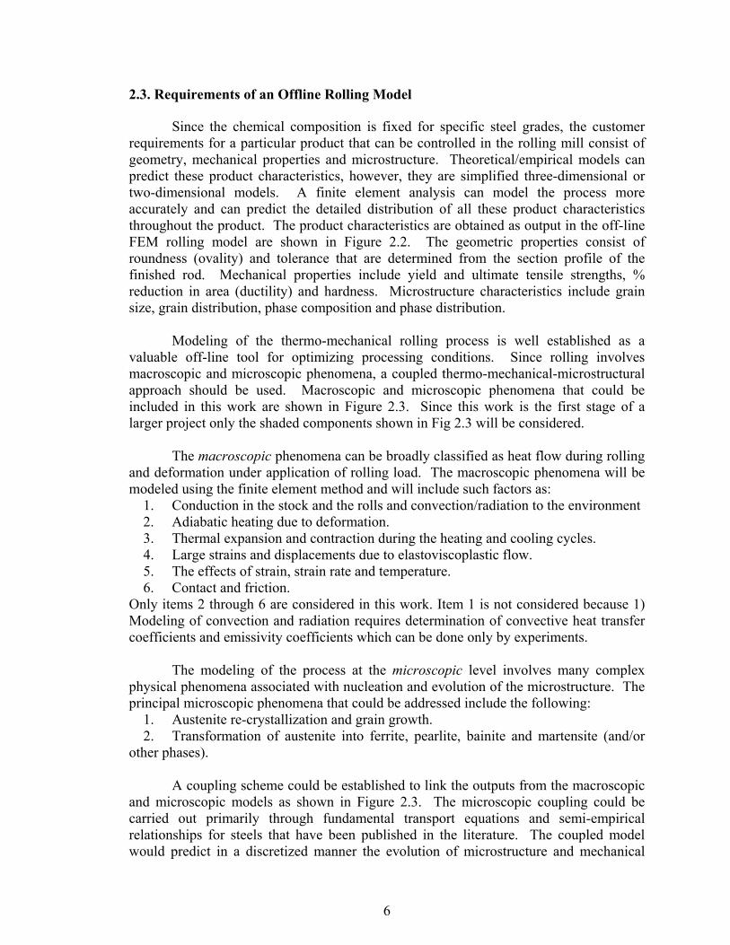
2.3. Requirements of an Offline Rolling Model
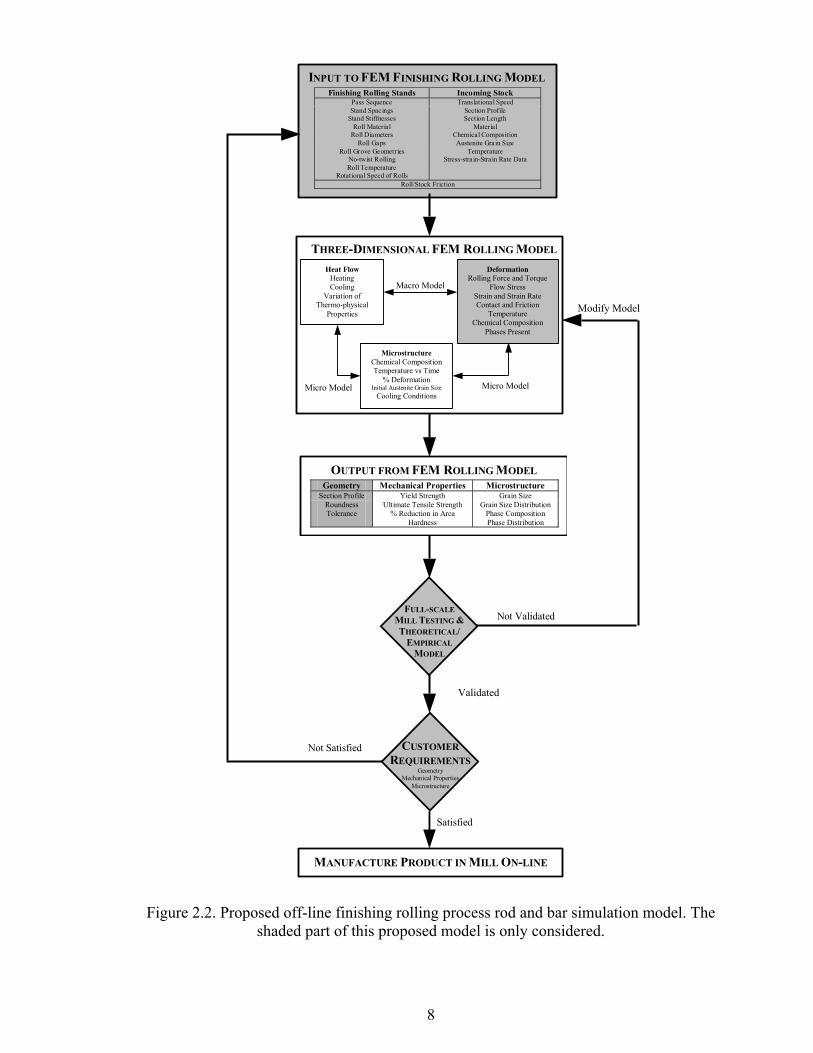
Since the chemical composition is fixed for specific steel grades, the customer requirements for a particular product that can be controlled in the rolling mill consist of geometry, mechanical properties and microstructure. Theoretical/empirical models can predict these product characteristics, however, they are simplified three-dimensional or two-dimensional models. A finite element analysis can model the process more accurately and can predict the detailed distribution of all these product characteristics throughout the product. The product characteristics are obtained as output in the off-line FEM rolling model are shown in Figure 2.2. The geometric properties consist of roundness (ovality) and tolerance that are determined from the section profile of the finished rod. Mechanical properties include yield and ultimate tensile strengths, % reduction in area (ductility) and hardness. Microstructure characteristics include grain size, grain distribution, phase composition and phase distribution.
Modeling of the thermo-mechanical rolling process is well established as a valuable off-line tool for optimizing processing conditions. Since rolling involves macroscopic and microscopic phenomena, a coupled thermo-mechanical-microstructural approach should be used. Macroscopic and microscopic phenomena that could be included in this work are shown in Figure 2.3. Since this work is the first stage of a larger project only the shaded components shown in Fig 2.3 will be considered.
The macroscopic phenomena can be broadly classified as heat flow during rolling and deformation under application of rolling load. The macroscopic phenomena will be modeled using the finite element method and will include such factors as: 1. Conduction in the stock and the rolls and convection/radiation to the environment 2. Adiabatic heating due to deformation. 3. Thermal expansion and contraction during the heating and cooling cycles. 4. Large strains and displacements due to elastoviscoplastic flow. 5. The effects of strain, strain rate and temperature. 6. Contact and friction. Only items 2 through 6 are considered in this work. Item 1 is not considered because 1) Modeling of convection and radiation requires determination of convective heat transfer coefficients and emissivity coefficients which can be done only by experiments.
The modeling of the process at the microscopic level involves many complex physical phenomena associated with nucleation and evolution of the microstructure. The principal microscopic phenomena that could be addressed include the following: 1. Austenite re-crystallization and grain growth. 2. Transformation of austenite into ferrite, pearlite, bainite and martensite (and/or other phases).
A coupling scheme could be established to link the outputs from the macroscopic and microscopic models as shown in Figure 2.3. The microscopic coupling could be carried out primarily through fundamental transport equations and semi-empirical relationships for steels that have been published in the literature. The coupled model would predict in a discretized manner the evolution of microstructure and mechanical

7
properties at the finite element nodal points. The main assumption is that microstructural features and mechanical properties can be determined and assigned to each macroscopic nodal point. Therefore, a fine mesh will result in predicting the microstructure evolution with greater precision.
The proposed off-line three-dimensional FEM rolling model will be designed for usage as shown in Figure 2.2. In this work only the shaded boxes in Figure 2.2 are considered, however discussion will address all components. Inputs to the off-line FEM rolling model include specifications on the rolling mill finishing stands and incoming stock. The incoming stock is assumed to be at a uniform temperature and uniform austenite grain size. Once the rolling model has solved the coupled thermo-mechanical-microstructural problem, the predicted results are output as geometrical, microstructural, and mechanical properties. The numerical results of the FEM rolling model are then validated with full-scale mill testing and verified with current theoretical/empirical models. Theoretical/empirical models for rod and bar round-oval-round pass rolling can predict spread/side free surface [2.1, 2.3], section profile (cross-sectional area) [2.4], mean effective plastic strain and strain rate [2.5, 2.6], and roll force and torque (power) [2.7, 2.8]. If the FEM results are inconsistent with test and theoretical/empirical results, the model is modified. Once the FEM model is validated, the output is compared to customer requirements. If the FEM results do not satisfy customer requirements, the input conditions of the rolling process are modified. This refinement is repeated until the FEM solutions are consistent with the mill testing, theoretical/empirical models and customer requirements. When both these requirements are satisfied, the product would be considered suitable for production on-line.
2.4. Challenges in Developing an Off-line Rolling Model
Simulating high speed hot rolling of long products is considered one of the most difficult metal-forming processes and is very complicated from an analyst's perspective. The application of finite element approximations to the rolling process poses modeling challenges on the macroscopic and microscopic levels. Some of the macroscopic challenges include the following:
• Nonlinear Phenomena. The rolling process involves many nonlinear phenomena, e.g., high rates of deformation, contact, friction, rate dependent material behavior, heat transfer and thermo-mechanical coupling. Microscopic issues will not be considered in this work.
• Slender Stock. The large aspect ratio of the stock (length in the rolling direction versus the product cross-sectional dimensions) presents a challenge to adequately discretize the three-dimensional material and conduct the simulations economically.
• Process Interactions between Rolling Stands. Continuous mill operations are complicated further by the interaction of processing between multiple stands that are inherent in the mill design. For example, sensitivity of the deformation in long narrow product to the effects of tension and compression between rolling stands places demands on the accuracy of the boundary conditions and the computational techniques.
8
Figure 2.2. Proposed off-line finishing rolling process rod and bar simulation model. The
shaded part of this proposed model is only considered.
Modify Model
INPUT TO FEM FINISHING ROLLING MODELFinishing Rolling Stands Incoming Stock
Pass Sequence Translational Speed Stand Spacings Section Profile
Stand Stiffnesses Section Length Roll Material Material
Roll Diameters Chemical Composition Roll Gaps Austenite Grain Size
Roll Grove Geometries Temperature No-twist Rolling Stress-strain-Strain Rate Data Roll Temperature
Rotational Speed of Rolls Roll/Stock Friction
Heat Flow Heating Cooling
Variation of Thermo-physical
Properties
THREE-DIMENSIONAL FEM ROLLING MODEL
Deformation Rolling Force and Torque
Flow Stress Strain and Strain Rate Contact and Friction
Temperature Chemical Composition
Phases Present
Microstructure Chemical CompositionTemperature vs Time
% Deformation Initial Austenite Grain Size
Cooling Conditions Micro Model Micro Model
Macro Model
OUTPUT FROM FEM ROLLING MODEL Geometry Mechanical Properties Microstructure
Section Profile Yield Strength Grain Size Roundness Ultimate Tensile Strength Grain Size Distribution Tolerance % Reduction in Area Phase Composition
Hardness Phase Distribution
Not Validated FULL-SCALE
MILL TESTING & THEORETICAL/
EMPIRICAL MODEL
CUSTOMER REQUIREMENTS
Geometry Mechanical Properties
Microstructure
MANUFACTURE PRODUCT IN MILL ON-LINE
Satisfied
Not Satisfied
Validated

9
Figure 2.3. Coupling scheme for macroscopic and microscopic models. 2.5. Rod and Bar Rolling Simulation Codes used by the Overseas Steel Industry
This section provides a brief state-of-practice review of rolling simulation codes
and steel microstructure models encountered in the worldwide steel industry. A literature review on the current state-of-practice reveals very little detailed information regarding the theoretical aspects of any existing thermo-mechanical microstructure rod and bar rolling simulations since they are all proprietary in nature. There are currently no commercial codes in the marketplace that specialize on rolling simulations. ABAQUS [2.9] and MSC.Marc [2.10] have been used extensively to analyze the rolling process whereas ADINA [2.11], ANYSY [2.12], DEFORM-3D [2.13], FORGE3 [2.14], LS-DYNA [2.15] and MSC.SuperForge (finite volume) [2.16] are mainly used for sheet metal forming and forging applications. However, there are non-commercial finite element rolling codes that have been developed for the steel industry in Japan, Germany and the United Kingdom as shown in Table 2.3. None of them are available for use in the U.S.
The two Japanese codes include CORMILL and SIMURO. The CORMILL (COmputational Rolling MILL) System [2.17-2.18] was developed at the University of Tokyo, however it can only be used by a Japanese company/university. The CORMILL System is based on mixed Lagrangian-Eulerian formulation assuming elastic-plastic material behavior. CORMILL is capable of simulating three-dimensional deformation characteristics and microstructure evolution in the hot rolling of strip, bar, and wire rod. Development started in 1989 and the developers claim that there have been more than several thousand case studies carried out at University of Tokyo and Japanese industries. The CORMILL System is used today as a tool to design new rolling conditions, roll groove profiles and operation conditions in the research and development departments of several Japanese companies.
Daido Steel, a private steel producer in Japan has independently developed SIMURO (SIMUrator for ROlling) [2.20] to analyze rolling, however, it also is not in the public domain. SIMURO is a three-dimensional, thermo-mechanical finite element based code assuming rigid-plastic material behavior. The major difference between the Japanese programs is that SIMURO can simulate the entire rolling process including the cooling zone that is not considered in CORMILL. Theoretical aspects and capabilities of SIMURO cannot be found in the literature. SMS Scholoemann-Siemag AG a German manufacturer of rolling mill equipment has developed an in-house computer simulation coupled with MSC.Marc called CRCT
Microscopic ModelT(A3), T(A1),
D0,f α, fcarbide , fγ,
Τ heating , T cooling & (dT/dt)cooling
Macroscopic Model Heat Flow Deformation T(t), k, C p , h, σ r , α , & dT/ dt ε p , d ε p / dt, σ
& µ
Coupling SchemeRelationships betweenT(t), εp, dεp/dt, D0 & t0.5
D0 &
Fraction Transformed
T(t), dT/dt, εp,dεp/dt &
Stock Dimensions
THREE-DIMENSIONAL FEM R OLLING MODEL

10
[2.20,2.21], i.e., Controlled Rolling and Cooling Technology, which has been around since 1991. CRCT is used by SMS to further develop rolling technology and by rod mill operators in Europe to improve final product quality. The software simulates the temperature evolution of a rod through a rolling mill and predicts the microstructure and mechanical properties of the rolled stock. In the literature a very brief description of code capabilities can be found and no information is provided on theoretical aspects.
Corus (part of which was formerly British Steel) is one of the United Kingdom's largest steel producers and 80% of its products are hot rolled. The Corus research and development group in the U.K. is at Swinden Technology Centre and this center has the ability to predict shape and property development during hot rolling, cooling and downstream processing via simulation [2.22,2.23]. Corus has been applying the finite element technology to solve various processes types, e.g., forming, welding, etc., since 1978. Current software includes finite element components developed in-house and other commercial finite element codes used along side ABAQUS.
Table 2.3. Comparison of overseas rod and bar rolling simulation codes.
REFERENCE CORMILL [2.17-2.19] SIMURO [2.20] CRCT
[2.21,2.22] Corus
[2.23,2.24] COUNTRY Japan Japan Germany United Kingdom
COMPUTER CODE In-House In-House &
MSC.Marc In-House & MSC.Marc
In-House & ABAQUS
USER INTERFACE Command Graphical Graphical Graphical
TECHNIQUE Finite Element Finite Element Finite Element Finite Element
FORMULATION Arbitrary
Lagrangian-Eulerian
Arbitrary Lagrangian-
Eulerian
Arbitrary Lagrangian-
Eulerian
Arbitrary Lagrangian-
Eulerian DIMENSIONALIT
Y 3-D 1-D, 2-D & 3-D 3-D 3-D
TIME DEPENDENCE
Steady-State & Transient
Steady-State & Transient
Steady-State & Transient
Steady-State & Transient
MATERIAL MODEL Elasto-Plastic Rigid-Plastic Elasto-Plastic Elasto-Plastic &
Visco-Plastic
MATERIAL FLOW STRESS
Misaka's Equation &
General Equation
12 Types (Unknown) & User Defined
Plastic Strain, Plastic Strain
Rate & Temperature
Strain, Strain Rate & Temperature
THERMO-MECHANICAL
COUPLING No Yes Yes Yes
COOLING No Yes Yes Yes ROLL
MATERIAL Rigid & Elastic Unavailable Unavailable Rigid & Elastic
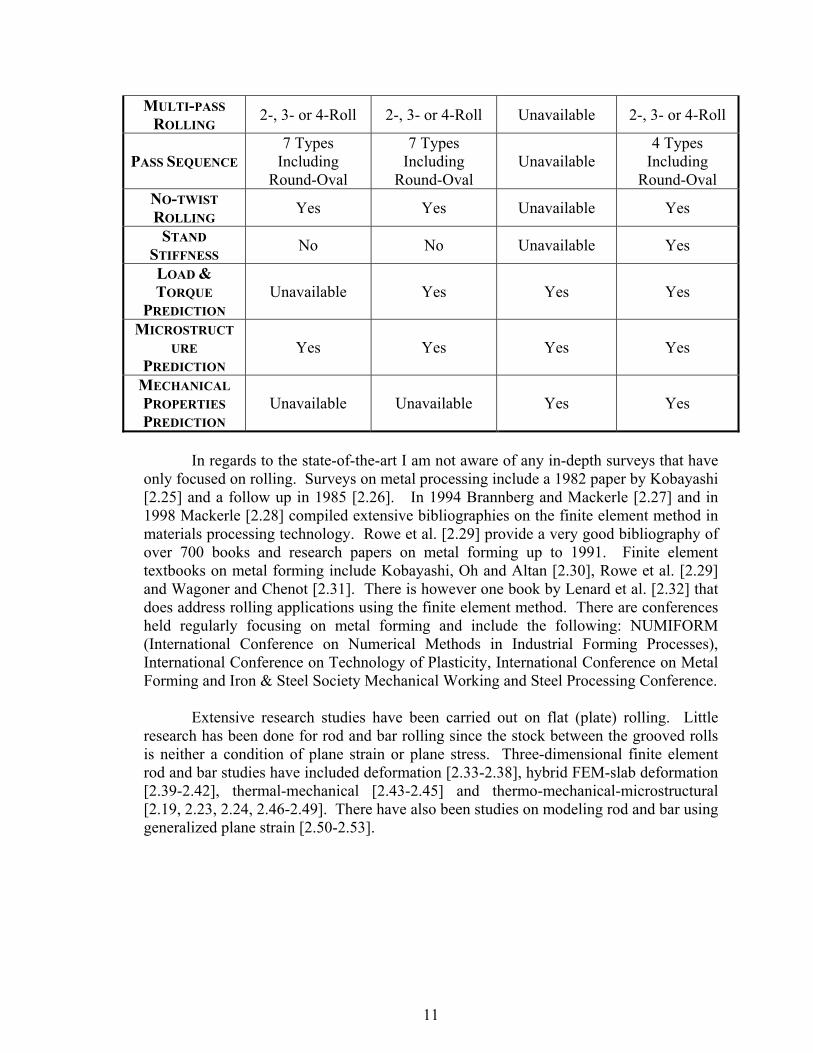
11
MULTI-PASS ROLLING 2-, 3- or 4-Roll 2-, 3- or 4-Roll Unavailable 2-, 3- or 4-Roll
PASS SEQUENCE 7 Types
Including Round-Oval
7 Types Including
Round-Oval Unavailable
4 Types Including
Round-Oval NO-TWIST ROLLING Yes Yes Unavailable Yes
STAND STIFFNESS No No Unavailable Yes
LOAD & TORQUE
PREDICTION Unavailable Yes Yes Yes
MICROSTRUCTURE
PREDICTION Yes Yes Yes Yes
MECHANICAL PROPERTIES PREDICTION
Unavailable Unavailable Yes Yes
In regards to the state-of-the-art I am not aware of any in-depth surveys that have
only focused on rolling. Surveys on metal processing include a 1982 paper by Kobayashi [2.25] and a follow up in 1985 [2.26]. In 1994 Brannberg and Mackerle [2.27] and in 1998 Mackerle [2.28] compiled extensive bibliographies on the finite element method in materials processing technology. Rowe et al. [2.29] provide a very good bibliography of over 700 books and research papers on metal forming up to 1991. Finite element textbooks on metal forming include Kobayashi, Oh and Altan [2.30], Rowe et al. [2.29] and Wagoner and Chenot [2.31]. There is however one book by Lenard et al. [2.32] that does address rolling applications using the finite element method. There are conferences held regularly focusing on metal forming and include the following: NUMIFORM (International Conference on Numerical Methods in Industrial Forming Processes), International Conference on Technology of Plasticity, International Conference on Metal Forming and Iron & Steel Society Mechanical Working and Steel Processing Conference.
Extensive research studies have been carried out on flat (plate) rolling. Little research has been done for rod and bar rolling since the stock between the grooved rolls is neither a condition of plane strain or plane stress. Three-dimensional finite element rod and bar studies have included deformation [2.33-2.38], hybrid FEM-slab deformation [2.39-2.42], thermal-mechanical [2.43-2.45] and thermo-mechanical-microstructural [2.19, 2.23, 2.24, 2.46-2.49]. There have also been studies on modeling rod and bar using generalized plane strain [2.50-2.53].

12
3. Theoretical and Empirical Geometric and Deformation Models for Steel Rod and Bar Round-Oval, Oval-Round Pass Rolling
3.1. Overview
Theoretical and empirical rolling models are a valuable alternative in validating full-scale mill testing and verifying the finite element-rolling model. Theoretical and empirical models to predict geometric and deformation parameters are well established for strip and plate rolling, however, forming conditions in rod and bar rolling is three-dimensional and the former is two-dimensional. In this chapter the state-of-the-art of theoretical and empirical models for rod and bar round-oval-round rolling will be discussed. The major advantage of these models is their simplicity and fast computational time to obtain a solution. Furthermore, these models are fairly accurate in calculating certain parameters of the rod/bar rolling process and the rolled products. However, these models do not provide detailed information about how a parameter varies throughout the rod/bar length and cross section and in that sense can only yield limited global information. The geometric and deformation models that will be discussed include spread and side free surface, section profile (cross-sectional area), mean effective plastic strain and strain rate, and roll force and torque (power). 3.2. Spread and Cross-sectional Area
Several empirical analytical models have been proposed to calculate the surface profile and side free surface of a deformed rod and bar stock. Spread is defined as the dimension of the deformed stock after rolling in the direction normal to the direction of rolling (perpendicular to paper) as shown in Figure 3.1. In other words, it measures the increase of width of the stock due to rolling deformation. The side free surface is defined as the region of the stock surface that does not come in to contact with the rolls during the rolling process as signified by the thick line in Figure 3.1.
Figure 3.1. Spread and side free surface.

13
The spread and side free surfaces are very important in rolling. The surface profile of a deformed stock depends on the spread, free surface profile, and the elongation of the stock. This means that the final shape of the stock is mainly dependent on these parameters. Since the final shape of the stock is very important to the customer, these parameters are very crucial to a roll pass designer when designing a particular rolling pass for specific shape and size requirements. Accuracy in calculating these parameters are critical when satisfying such geometric customer requirements as roundness and tolerance in accordance with ASTM standards [3.1]. Roundness is defined as the difference between maximum diameter and minimum diameter. Tolerance is the allowable difference in maximum/minimum diameter between what a customer orders and what the steel mill delivers.
Table 3.1 provides a comparison of various spread and side free surface models. The main disadvantages of the following models are stated in the table. The three most widely used models in practice will be discussed and have been developed by Saito et al. [3.2], Arnold and Whitton [3.3] and Shinokura and Takai [3.4].
Saito et al. [3.2], in 1977, proposed empirical formulas for calculating spread. The model depends on such parameters as theoretical contact width, actual contact width, mean thickness of the stock, mean height of the pass, mean radius of the roll, mean projected contact length, projected contact area, spread coefficient, elongation coefficient and mean forward slip rate. The major assumption is that the shape of the free surface before and after the rolling is same. The model was experimentally verified by carrying out tests on mild steel S17C (0.17%C, 0.19%Si, 0.47%Mn, 015%P, 0.029%S, 0.008%Al) at 1050+100 oC.
Arnold and Whitton [3.3], in 1975, proposed a simple empirical model where spread is calculated based on calculation of a spread coefficient. This model uses an experimental factor and thickness of the rectangle the same cross-sectional area as the rod section before and after rolling. The model was experimentally verified using titanium 120,130, and 160, mild steel and titanium alloys 314,315,317 and 318. The main disadvantage of this model is that there are too many unknowns and to solve for spread one has to assume a final cross-sectional area. Therefore, this approach can only be used for experimental verification not pass design. Furthermore, it doesn’t take into account the finish round stands encountered in Morgan RSM mill.
Shinokura and Takai [3.4], in 1982 developed an empirical-theoretical model that
calculates maximum stock spread in round-oval (or oval-round) pass and square-diamond (or diamond-square) pass rolling. The idea behind this model is that the maximum spread of an outgoing stock can be calculated from the roll radius, maximum size of incoming stock and the area fraction between stock and the geometry of the roll groove. The parameters used in this model are initial width (Wi), mean radius of the roll (Rmean), equivalent height of incoming stock (Hi), equivalent height of outgoing stock (Ho),

14
maximum height of stock (hi) and the spread coefficient (γ). The spread Wmax is determined from the following relationship,
( )max 1
0.5mean i oh
io i i
R H HAW WA W h
γ − = + +
(3.1a)
with
( ) csoi BAAH −= (3.1b) ( )o o s h cH A A A B= − − (3.1c)
where Bc is the interval of two cross points perpendicular to the roll axis direction when the stock cross-section and roll-groove overlap, Ao is the cross-sectional area of incoming stock, Ah is the area fraction of stock above roll-groove when the cross-section of the stock and roll-groove are overlapped, and As is the area fraction of stock cut out by Bc at the inside roll-groove when the cross-section of the stock and roll-groove overlap. The parameters are shown in Figure 3.2. The important assumption is that the spread of the stock depends only on the geometry of the stock and roll-groove. The main disadvantage of the model is the empirical spread coefficient, which are determined by experiment. The value of the spread coefficient in oval-round pass is 0.83 and in round-oval pass is 0.97.
Lee et al. [3.22], in 2000, proposed an empirical model where free surface radius is calculated based on calculation of spread by Shinokura and Takai [3.4]. This model is valid only for round-oval and oval-round pass sequences. This model linearly interpolates between groove radius and stock radius and uses a weighting fraction based on spread and face width. The model is experimentally validated for low carbon plain steel (0.1%C) in a experimental mill setup.
Shinokura and Takai’s [3.4] model is used in this work for calculating spread
because it is fairly accurate in most conditions. This model is also well accepted in industry. And many research efforts are based on this model. For calculation of surface profile Lee et al. [3.22] used this model.

15
Figure 3.2. Illustration of equivalent rectangle method in round-oval pass for calculation
of equivalent height of incoming stock and roll groove.

16
Table 3.1. Models for determining spread and side free surface.
NA=Not Available CR=Cannot Read Since written in Languages other than English
Reference Theoretical/ Empirical
Model
Experimental Verification Steel Type(s)
Pass Sequence
Transnational Rolling
Speed
Rolling Temperature Disadvantages Comments
Arnold and Whitton [3.3] Empirical Yes
Pure Titanium (120,130,160), Mild Steel and
Titanium Alloys (314,315,317,318)
NA NA
700 & 800 oC: Titanium
900 oC:
Mild Steel
- No Discussion on Spread Equation
- Round-oval Pass Sequence Not
Considered - Spread is based on
calculation of exit area experimentally.
Saito et al. [3.2] Empirical Yes Mild Steel S17C NA NA 1050 + 100 oC
- Assumes shapes of free surface before and after
rolling are same. + 2-3 % Error
Schlegel and Hensel [3.7] NA NA NA NA NA NA NA
Shinokura and Takai [3.4]
Empirical-Theoretical Yes Mild NA NA 950 - 1050 oC
- Spread formula uses a coefficient that needs
more verification.
Vater and Schütza [3.6] Empirical Yes NA NA NA
- Not General - Not Simple
- Not Accurate
Yanagimoto [3.5] Empirical Yes CR NA NA 1100 oC CR
Lee et al. [3.22] Empirical Yes Low carbon Steel
(0.1%C)
Single Stand Experimental
Mill NA 1400 oC
- Calculation of Surface Profile
- Valid for Round-oval and Oval-round Pass

17
3.3. Mean Effective Plastic Strain
The mean effective plastic strain at a rolling stand is defined as the maximum average effective (equivalent) plastic strain of the stock at a given stand during the rod/bar rolling process. Calculation of mean effective plastic strain is extremely important for predicting and controlling the mechanical properties of the rod/bar after rolling because all mathematical models of microstructure evolution requires thermo-mechanical variables such as mean effective plastic strain, mean effective plastic strain rate and temperature at each rolling stands. Temperature evolution due the mechanical energy converted to heat during the deformation process is also dependent on mean effective plastic strain and mean effective plastic strain rate. Furthermore, mean effective plastic strain rate is in turn a function of mean effective strain and the process time. All of this suggests that the capability of predicting mean plastic strain is essential for controlling the mechanical properties and microstructure of the output rod/bar.
Mean effective plastic strain can be defined in two ways:
1. Incremental mean effective plastic strain. Here it is assumed that the geometry of the stock before it enters a particular stand is the initial geometry of the stock. The final geometry of the stock is the geometry after a particular stand.
2. Total mean effective plastic strain. Here it is assumed that the geometry of the stock before it enters the 1st stand is the initial geometry of the stock. The final geometry of the stock is the geometry after a particular stand.
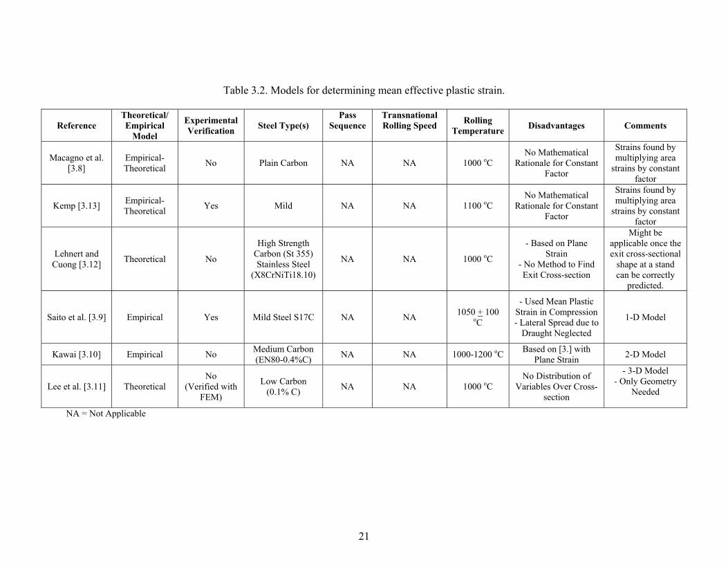
Table 3.2 provides a comparison of various mean effective strain models. The main advantages and disadvantages of each model are stated in this table. The three most widely used models in practice will be discussed and have been developed by Macagno et al. [3.8], Saito and Kawai [3.9,10] and Lee et al. [3.11]. Macagno et al. [3.8], in 1996 proposed an empirical model of calculating mean effective strain as simple area strains multiplied by an empirical factor. This model is validated against the numerical simulation of deformation due to rod rolling developed at BHP steel [3.13] to calculate the redundant strains associated with specific groove geometries. The main disadvantage of this model is the significant variation of the empirical factor, which ranges from 1.5 to 2 in the roughing stands and 2 to 3 in the subsequent finishing stands.
Saito et al. [3.9], in 1983 proposed a model for mean strain based on equivalent rectangle approximation method discussed before for calculation of spread by Shinokura and Takai [3.4] method. According to Saito et al. [3.9] mean effective plastic strain is expressed simply as natural logarithmic of change of equivalent height on the basis of cross point of incoming stock and groove shape of rolls i.e.,
=
o
ip
HHlnε (3.2a)

18
where Hi is height of the initial equivalent rectangle and Ho is height of the final equivalent rectangle.
Kawai [3.10], in 1985, adopted Saito et al.’s [3.10] equation but included a constant in Equation (3.2a). He introduced this constant by applying the plane strain condition in the case of rolling process. His equation is given as,
=
o
ip
HHln
32ε (3.2b)
Lee et al. [3.11], in 1999, proposed a model based on equivalent rectangle approximation method and hypothesis of parallelepiped deformation. In this model the round or oval Stock is replaced by a equivalent rectangular prism (Figure 3.3). Then principal plastic strain components are calculated using the volume constancy criteria. The parameters used in this model are equivalent height of initial geometry of the stock (Hi), equivalent height of final geometry of the stock (Ho), equivalent width of initial geometry of the stock (Wi), equivalent width of final geometry of the stock (Wo). The strain is given by
( )2 21 2 1 2
23pε ε ε ε ε+= + (3.3a)
1 ln i
o
HH
ε =
(3.3b)
2 ln i
o
WW
ε =
(3.3c)
Three methods of maximum height, method of maximum width, method of width-height ratio can be used for calculating the parameters Hi, Ho, Wi, Wo.
In maximum height method the maximum height of the stock both initial and final is chosen as Hi and Ho. The widths, Wi and Wo is calculated the following relationships
ii
i
AWH
= (3.3d)
oo
o
AWH
= (3.3e)
where Ai and Ao are initial and final areas of the stock. In maximum width method the maximum width of the stock both initial and final
is chosen as Wi and Wo. The heights, Hi and Ho is calculated the following relationships i
ii
AHW
= (3.3f)
oo
o
AHW
= (3.3g)
where Ai and Ao are initial and final areas of the stock.

19
In width-height ratio method an arbitrary ratio for both Wi /Hi and Wo /Ho is
assumed. Then Wi, Wo, Hi and Ho is calculated the following relationships i i iA H W= (3.3h)
o o oA H W= (3.3i) where Ai and Ao are initial and final areas of the stock. These methods of calculation are shown in Figure 3.4.
The major disadvantage of this model is that it assumes that the strain components
in x, y, z directions are actually the principal strain directions. Also, the error of this model also increases with the amount of distortion. However it is the most recent and most improved model for calculating strain. This model is used in conjunction with maximum width method for calculating theoretical effective plastic strain (both incremental and total) in this work. This is because maximum width method is shown to be most accurate with finite element solution by Lee et al. [3.11]. In case of both incremental and total mean effective plastic strain the initial parameters (Wi, Hi and Ai) are chosen according to their definition given above.
Figure 3.3. Schematic representation of parallelepiped deformation of equivalent
rectangle section (reprinted from Lee et al. [3.11]).

20
Figure 3.4. Three methods of computing an equivalent cross sectional area for the oval
round stand. (a) Method of width-height ratio (b) Method of maximum height (c) Method of maximum width (reprinted from Lee et al. [3.11]).
21
Table 3.2. Models for determining mean effective plastic strain.
Reference Theoretical/ Empirical
Model
Experimental Verification Steel Type(s)
Pass Sequence
Transnational Rolling Speed
Rolling Temperature Disadvantages Comments
Macagno et al. [3.8]
Empirical-Theoretical No Plain Carbon NA NA 1000 oC
No Mathematical Rationale for Constant
Factor
Strains found by multiplying area
strains by constant factor
Kemp [3.13] Empirical-Theoretical Yes Mild NA NA 1100 oC
No Mathematical Rationale for Constant
Factor
Strains found by multiplying area
strains by constant factor
Lehnert and Cuong [3.12] Theoretical No
High Strength Carbon (St 355) Stainless Steel
(X8CrNiTi18.10)
NA NA 1000 oC
- Based on Plane Strain
- No Method to Find Exit Cross-section
Might be applicable once the exit cross-sectional
shape at a stand can be correctly
predicted.
Saito et al. [3.9] Empirical Yes Mild Steel S17C NA NA 1050 + 100 oC
- Used Mean Plastic Strain in Compression - Lateral Spread due to
Draught Neglected
1-D Model
Kawai [3.10] Empirical No Medium Carbon (EN80-0.4%C) NA NA 1000-1200 oC Based on [3.] with
Plane Strain 2-D Model
Lee et al. [3.11] Theoretical No
(Verified with FEM)
Low Carbon (0.1% C) NA NA 1000 oC
No Distribution of Variables Over Cross-
section
- 3-D Model - Only Geometry
Needed
NA = Not Applicable

22
3.4. Roll Force
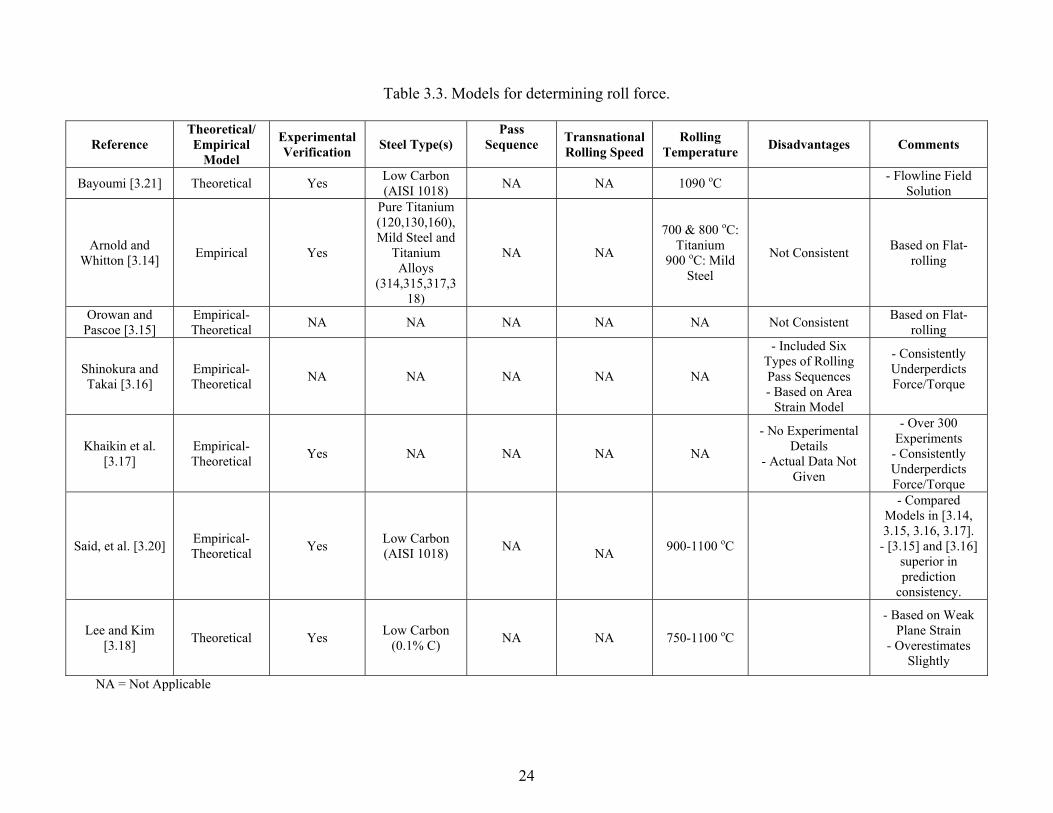
Calculation of roll force is important because calculation of torque and power in a rolling mill is based on calculation of roll force. Accurate prediction of roll force for grooved rolling is considerably more difficult than predicting the geometry of the stock. There are essentially three problems, present during flat rolling as well but somewhat easy to handle. They are 1) material’s resistance to deformation, as a function of strain, strain rate and temperature 2) the ability to calculate the distributions of the strains, strain rates, stress and temperature in the deformation zone and; 3) the conditions at the roll metal interface, i.e., the coefficients of friction and heat transfers. Table 3.3 provides a comparison of various roll force and torque models. The main disadvantages of each model are stated in this table. The five most widely used models in practice will be discussed and have been developed by Arnold and Whitton [3.14], Orowan and Pascoe [3.15], Shinokura and Takai [3.16], Khaikin et al. [3.17] and Lee et al. [3.18]
Arnold and Whitton [3.14], in 1975 proposed a formula for roll-separating force based on Sim’s [3.19] hot flat rolling theory, which included modifications for projected area of contact and empirical factors.
Orowan and Pascoe [3.15], in 1948 modified their simplified theory of flat rolling to be convenient for bar rolling. They assumed sticking friction for their model.
Shinokura and Takai [3.16], in 1986 introduced a method for calculating effective roll radius, the projected contact area, the non-dimensional roll force and the torque arm coefficients, which were expressed as simple functions of the geometry of the deformation zone. These variables are given for square-to-oval, round-to-oval, square-to-diamond, diamond-to-diamond and oval-to-oval stands.
Khaikin et al. [3.17], in 1971 developed a relation for the projected area of contact for square-diamond-square pass sequence.
Most recently Lee et al. [3.18], in 2001 developed a relation based on projected contact area and average contact stress (roll pressure). In this model it is assumed that deformation occurs under a weak plane strain condition. According to his model roll force at a given stand is calculated by the means of following equations
dF PA= (3.4a)
max02 1x
mC
dx
xA L dxC
= −
∫ (3.4b)
( )11 expmm
LP Khµε
= −
(3.4c)
where, F is roll force, P is roll pressure, L is average contact length, Lmax is maximum contact length Ad is total contact area, hm is effective mean height of stock, Km is average resistance

23
and µ is Coulomb friction co-efficient. In this study Lee et al. [3.18] model has been used for calculating roll force.
24
Table 3.3. Models for determining roll force.
Reference Theoretical/ Empirical
Model
Experimental Verification Steel Type(s)
Pass Sequence
Transnational Rolling Speed
Rolling Temperature Disadvantages Comments
Bayoumi [3.21] Theoretical Yes Low Carbon (AISI 1018) NA NA 1090 oC - Flowline Field
Solution
Arnold and Whitton [3.14] Empirical Yes
Pure Titanium (120,130,160), Mild Steel and
Titanium Alloys
(314,315,317,318)
NA
NA
700 & 800 oC: Titanium
900 oC: Mild Steel
Not Consistent Based on Flat-rolling
Orowan and Pascoe [3.15]
Empirical-Theoretical NA NA NA NA NA Not Consistent Based on Flat-
rolling
Shinokura and Takai [3.16]
Empirical-Theoretical NA NA NA NA NA
- Included Six Types of Rolling Pass Sequences - Based on Area
Strain Model
- Consistently Underperdicts Force/Torque
Khaikin et al. [3.17]
Empirical-Theoretical Yes NA NA NA NA
- No Experimental Details
- Actual Data Not Given
- Over 300 Experiments
- Consistently Underperdicts Force/Torque
Said, et al. [3.20] Empirical-Theoretical Yes Low Carbon
(AISI 1018) NA NA 900-1100 oC
- Compared Models in [3.14, 3.15, 3.16, 3.17].
- [3.15] and [3.16] superior in prediction
consistency.
Lee and Kim [3.18] Theoretical Yes Low Carbon
(0.1% C) NA NA 750-1100 oC
- Based on Weak Plane Strain
- Overestimates Slightly
NA = Not Applicable
25
4. Predicting Flow Stress Behavior of Steel at High Temperature and Strain Rates
4.1. Overview
One of the important parameters in modeling the simulation of high-speed high
temperature rolling is the flow-stress behavior of the particular steel grade. Flow stress is defined, as the instantaneous yield stress or true stress of a metal defined when a metal starts to undergo continuous plastic deformation. The two principal methods for accurately obtaining the flow stress of a particular grade of steel is direct experimental results and empirical constitutive equations. Empirical constitutive equations are often derived from the regression analysis of experimental data. Typically these equations define the flow strength of a material as a function of the variable considered important by the authors. Table 4.1 lists well-known experimental studies, independently, carried out by different researchers around the world. Table 4.2 shows the most commonly used and widely acceptable constitutive equations for steel, their applicability for different strain ranges, strain rate and temperature and their advantages and disadvantages. 4.2. Experimental Studies
Various researchers have carried out experimental studies regarding the flow
stress of common steel grades at various strain rates. The most widely used experimental studies are by Cook [4.1], Suzuki [4.2] and Stewart [4.3]. Flow stress data is generally presented as smooth plots of flow stress versus natural strain for various strain rates and temperature ranges.
Cook et al. [4.1] in 1957 carried out experiments for measuring flow stress data for low carbon, medium carbon and high carbon steel. Flow stress versus natural strain curves was presented for various steel grades between a temperature range of 900oC to 1200oC and strain rate range of 1.5s-1 to 100 s-1.
Suzuki et al. [4.2] in 1968 carried out experiments for measuring flow stress data for metals and alloys using cam-plastometer apparatus. This article presented flow stress versus natural strain curves for various steel grades between a temperature range of 800oC to 1200oC for three strain rates 0.3 s-1, 2 s-1, 10 s-1.
Stewart et al. [4.3] carried out experiments for measuring flow stress data for metals and alloys. This article presented flow stress versus natural strain curves for various steel grades between a temperature range of 700oC to 1200oC and a strain rate range of 0.4 s-1 to 140 s-1.

26
Table 4.1. Experimental studies for determining flow stress of steel for different temperature, strain and strain rate ranges.
Experimental Data
Temperature Range Strain Range Strain Rate Range Experimental
Procedure Comments
Cook [4.1] 900oC to 1200oC NA 1.5s-1 to 100 s-1 NA - Closely matched by Tomchick equation [4.4]. - Not matched well by Misaka equation [4.6].
Suzuki [4.2] 800oC to 1200oC 0-70% 0.3 s-1, 2 s-1, 10 s-1 Cam-plastometer
- Closely matched by Tomchick equation [4.4]. - Not matched well by Misaka equation [4.6] for
low and high carbon steels. - Matched well by Shida equation [4.5] for low
carbon steel.
Stewart [4.3] 700oC to 1200oC NA 0.4 s-1 to 140 s-1 NA - Closely matched by Shida equation [4.5].
- Not matched well by Misaka [4.6] and Tomchick [4.4] equations.
NA=Not Available

27
4.3. Empirical Constitutive Equations Most of the empirical constitutive equations are based on the thermodynamical
concept that flow stress of a material depends on present values and past history of observable variables such as strain, strain rate and temperature. The general relationship is of the following form ( )Tf ,,εεσ = (4.1) where σ is the flow stress, ε is the strain, ε is the strain rate, T is the temperature and the exact relationship between the variables are determined by the regression analysis of available experimental data. The most widely used empirical equations have been developed by Tomchick [4.4], Shida [4.5] and Misaka [4.6]. Lee et al. [4.8] has recently proposed a modification of the Shida equation.
Tomchick [4.4], in 1982 proposed a empirical constitutive equation by studying Cook experimental data [4.1]. The experimental data was analyzed to determine strain hardening behavior, strain rate hardening behavior and temperature dependence by considering flow stress (σ) as a simultaneous function of strain (ε ), strain rate (ε ), and temperature (T). The equation is given by,
( ) ( )TBA mn λεεεσ −+= exp (4.2) where A, B, n, m and λ are material constants determined by regression analysis of the Cook experimental data [4.1].
Shida [4.5], in 1969 developed a constitutive equation, which is most comprehensive and widely used constitutive equations of steel. The relationship defines flow strength (σ) as a function of strain (ε ), temperature (T) and carbon content. The mathematical formulations of Shida’s empirical relations are as follows
10
m
f f εσ σ =
(in Kg/mm2) (4.3a)
where
5 0.010.28exp0.05f t C
σ = − + (4.3b)
( ) ( )0.019 0.126 0.075 0.05m C t C= − + + − (4.3c)
( ) 5 0.010.28 , exp0.05f
d
q C tt C
σ
= − + (4.3d)
( ) ( ) ( ) 20.95 0.49 0.06, 30 0.9
0.42 0.09C Cq C t C t
C C+ +
= + − + + + (4.3e)
( ) ( ) 0.0270.081 0.154 0.019 0.2070.320
m C t CC
= − + − + ++
(4.3f)
with, ( )0.95 0.41
0.32d
Ct
C+
=+
(4.3g)
dt t≥
dt t≥

28
1.3 0.30.2 0.2
n
f ε ε = −
(4.3h)
0.41 0.07n C= − (4.3i) ( ) /1000ot T K= (4.3j)
furthermore, C is the carbon content of the steel grade in percent and t is a dimensionless temperature.
Lee et al. [4.8] in 2002 modified Equation (4.3a) of Shida’s Model to make it more generalized and applicable to a much larger range of strain rates. The relationship in Equation (4.3a) is replaced by the following relationship
/ 2.4 /15
10 100 1000
m m m
f f ε ε εσ σ =
(4.4)
with all other parameters remaining the same as in [4.5]. Equation (4.4) is valid for the strain rate up to 3000s-1and has been validated by Split Hopkinson pressure bar test for 4340-alloy steel.
Misaka et al. [4.6] in 1971 developed a constitutive equation, which defines flow strength as a function of strain (ε ), strain rate (ε ), temperature (T), and material composition. The flow stress is given by the following relationship
22 0.21 0.132851 2968 1120exp 0.126 1.75 0.594 C Cf C C
Tσ ε ε
+ − = − + +
(4.5a)
0.916 0.18 0.389 0.191 0.004f Mn V Mo Ni= + + + + (4.5b) where σ is mean resistance to deformation (Kg/mm2), C is Carbon Content (%), Mn is Manganese Content (%), V is Vanadium Content (%), Mo is Molybdenum Content (%), Ni is Nickel Content (%), and T is temperature (o K).

29
Table 4.1. Constitutive equations for determining flow stress of steel for different strain rates and temperatures.
Constitutive Equation
Temperature Range
Strain Range
Strain Rate Range Material Composition Advantages Disadvantages
Tomchick [4.4] 900oC to 1200oC NA 1.5s-1 to 100 s-1 Low Carbon, Medium
Carbon and High Carbon Steel
- Matches excellently with Cook [4.1] data. - Applicable over a
wide variety of strain rates.
- Applicability of strain range is unclear.
- Effect of material composition is unclear.
Shida [4.5] 700oC to 1200oC 0-70% 1 s-1 to 100 s-1 Up to 1.2% Carbon Content
- Matches relatively well with Cook [4.1] and Suzuki [4.2] data.
- Effect of material composition on flow stress is well defined
Misaka [4.6] NA NA NA NA - Effect of material
composition on flow stress is well defined.
- Matches poorly with Suzuki [4.2] data form low and High Carbon
Steel.
Lee (Modified Shida)
[4.8] 25oC to 1100oC 0-70% 1 s-1 to 3000 s-1 Up to 1.2%
Carbon Content
- Matches excellently with SHPB test
conducted by Lee et al. [4.8]
- Applicable for a large range of strain
rate.
- Experimental verification has been done only for AISI
4340 steel.
NA= Not Available

30
5. Case Studies and Discussion 5.1. Overview
In this work the commercial finite element code ABAQUS/Explicit [5.1] is used to simulate the rolling process. Two case studies are considered as benchmarks to validate the finite element model against full-scale mill testing and theoretical models. The following two case studies are considered:
• Republic Engineered Products Rod Outlet. Republic Engineered Products, Lorain, OH, Rod Outlet is a single strand mill designed and installed by Morgan Construction Company and it began operating in 1994. It is a 14-stand outlet with 10-stand No-Twist Mill and 4-stand Reducing/Sizing mill. The mill now produces carbon and alloy steel rods from 5.5 mm to 22 mm diameter.
• POSCO No. 3 Mill. POSCO, No. 3 mill, Pohang, Korea is a two-strand mill, designed and installed by Morgan Construction Company and it began operating in 1988. Morgan upgraded the mill, in 2001. The initial 13 stands of this mill is double strands. The mill separates after stand 13 into two independent strands with 6-stand pre-finishing mills, 10-stand No-Twist mills and 4-stand Reducing/sizing mills. The mill now produces carbon and alloy steel bars from 5.0 mm to 22 mm diameter at temperatures as low as 750 oC, and at speeds of up to 110 meters per second. As a result of the upgrade, the output for the two strands will increase from 700,000 to 820,000 metric tons per year.
Details of these two case studies are given in Table 5.1. Table 5.1. Details of Republic Engineered Products Rod Outlet and POSCO No. 3 mill.
Organization REP (Republic Engineered Products) POSCO
Location Lorain, Ohio, USA Pohang, Republic of Korea
Built 1960s - Rod Outlet Added in 1994 1987 - Modernization with RSM’s in 2001
Mill Rod Outlet - Single Strand, 14 Stand Rod Outlet
Two strand, with 13 Stands Rolling Double Strand, Separating after Stand 13 into Two Independent Strands with Pre-finishing Mills,
No-Twist Mills and Reducing/Sizing Mills
Mill Arrangement
Rod Outlet - 10 Stand No-Twist Mill and 4 Stand Reducing/Sizing Mill
5-stand Roughing Mill, 8-stand Intermediate Mill, 6-stand Pre-
Finishing Mills, 10-stand No-Twist Mills and 4-stand Reducing/Sizing
Mills
Products Rod Outlet - Carbon and Alloy Steel
Rods from 5.5 mm to 22 mm Diameter
Carbon and Alloy Steel Bars from 5.0 mm to 22 mm Diameter
Billet 152 mm Square, Continuous Cast 162 mm Square, Continuous Cast

31
The Republic mill will consider the finishing stands (4-stand Reducing/Sizing
mill) while POSCO No.3 will consider the roughing stands (Initial four stands of the roughing mill). Since available finite element and theoretical results for POSCO No.3 mill can be found in Lee et al. [5.1, 5.3], the roughing stands are considered.
This chapter contains a brief description of these two case studies, the different techniques used to model the case studies, results of the finite element solution and a comparison of these results with available full-scale mill testing data and theoretical results. The two case studies will be presented based on the flow chart in Figure 2.2.
5.2. Case Study #1- Republic Engineered Products, Finishing Stands 5.2.1. Product Manufactured in the Mill The Republic Engineered Products, Lorain, OH consists of Morgan RSM [5.11] that is used to produce a finished rod of 12.75 mm diameter. The customer (rod user) is a U.S. automotive supplier who manufactures M12 x 1.25, 4g (high accuracy, fine fits) steel bolt of SAE class 4.6 from the finished rod. The material considered is AISI 1045 medium carbon steel that is commonly used in the U.S. automotive industry for gears, shafts, axles, studs and bolts. 5.2.2. Configuration of the Rolling Stands
The details of the Republic Engineered Products, Lorain, OH for the finishing rolling stands and the incoming stock are defined in Table 5.2. The geometric details regarding the finishing rolling stands were obtained from Morgan Construction Company [5.11]. Detailed pictures of the Republic Engineered Products RSM mill are shown in Figure 5.1. Republic Engineered Products RSM mill consists of four finishing stands with a pass sequence of oval-round-round-round. Stand #1 consists of two oval grooved rolls and input stock is of circular cross-section (Figure 5.1c). Stand #2 consists of two round grooved rolls oriented at 90o to Stand #1 and the output of the Stand #1 is used as input stock for this stand. Stand #3 consists of two round grooved rolls oriented at 90o to Stand #2 and the output of the Stand #2 is used as input stock for this stand. Stand #4 consists of two round grooved rolls oriented at 90o to Stand #3 and the output of the Stand #3 is used as input stock for this stand.
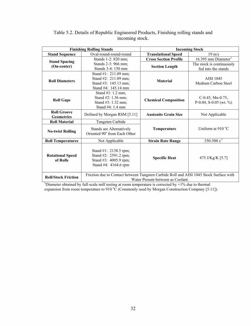
32
Table 5.2. Details of Republic Engineered Products, Finishing rolling stands and incoming stock.
Finishing Rolling Stands Incoming Stock
Stand Sequence Oval-round-round-round Translational Speed 19 m/s Cross Section Profile 16.395 mm Diameter1
Stand Spacing (On-center)
Stands 1-2: 820 mm; Stands 2-3: 966 mm; Stands 3-4: 150 mm Section Length The stock is continuously
fed into the stands
Roll Diameters
Stand #1: 211.09 mm; Stand #2: 211.09 mm; Stand #3: 145.13 mm; Stand #4: 145.14 mm
Material AISI 1045 Medium Carbon Steel
Roll Gaps
Stand #1: 1.2 mm; Stand #2: 1.36 mm; Stand #3: 1.32 mm; Stand #4: 1.4 mm
Chemical Composition C-0.45, Mn-0.75, P-0.04, S-0.05 (wt. %)
Roll Groove Geometries Defined by Morgan RSM [5.11] Austenite Grain Size Not Applicable
Roll Material Tungsten Carbide
No-twist Rolling Stands are Alternatively Oriented 90o from Each Other
Temperature Uniform at 910 oC
Roll Temperatures Not Applicable Strain Rate Range 350-500 s-1
Rotational Speed of Rolls
Stand #1: 2138.5 rpm; Stand #2: 2591.2 rpm; Stand #3: 4005.9 rpm; Stand #4: 4164.6 rpm
Specific Heat 475 J/Kg/K [5.7]
Roll/Stock Friction Friction due to Contact between Tungsten Carbide Roll and AISI 1045 Stock Surface with Water Present between as Coolant.
1Diameter obtained by full-scale mill testing at room temperature is corrected by +1% due to thermal expansion from room temperature to 910 oC (Commonly used by Morgan Construction Company [5.11]).
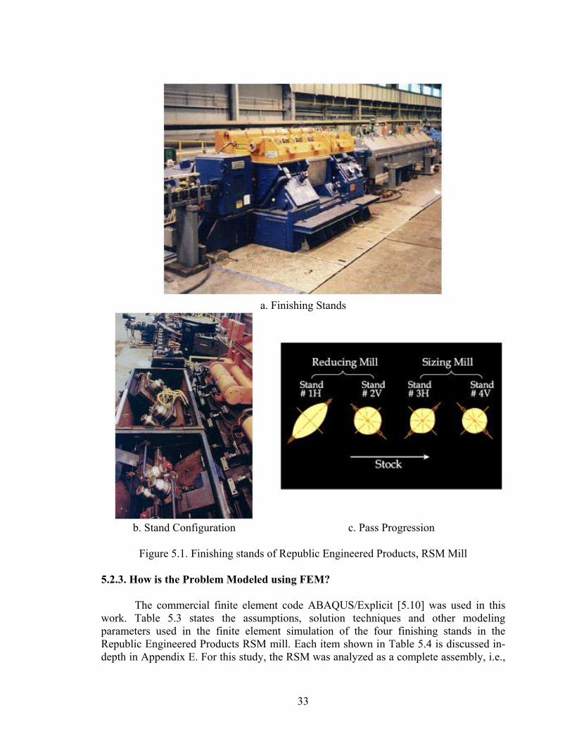
33
a. Finishing Stands
b. Stand Configuration c. Pass Progression
Figure 5.1. Finishing stands of Republic Engineered Products, RSM Mill
5.2.3. How is the Problem Modeled using FEM?
The commercial finite element code ABAQUS/Explicit [5.10] was used in this
work. Table 5.3 states the assumptions, solution techniques and other modeling parameters used in the finite element simulation of the four finishing stands in the Republic Engineered Products RSM mill. Each item shown in Table 5.4 is discussed in-depth in Appendix E. For this study, the RSM was analyzed as a complete assembly, i.e.,

34
all four stands as shown by the finite element model in Figure 5.2. A finite element pre- and post-processor program is written using Python script and Java (Appendix A) to analyze the results of the finite element solution and verify with full-scale mill testing data and validate with theoretical results.
Table 5.3. Details of ABAQUS/Explicit finite element model for the Republic Engineered Products, Finishing rolling stands and incoming stock.
Mesh Domain Lagrangian
Time Dependence Transient
Time Integration Explicit, Dynamics, Adiabatic.
Optimal time step is decided automatically by ABAQUS
Dimensionality Three-Dimensional Mass Scaling None
Adaptive Meshing Lagrangian Analysis: No
Formulation
Hourglass Artificial Stiffness
Element Type Linear Hexahedral Brick (C3D8R), Deformable, Reduced Integration
Mesh Characteristics
#of Nodes: 49,994 #of Elements: 48,820
#of DOF: 147,030 (including Lagrange Multipliers)
Material Homogeneous and Isotropic Length 1.0 m1
Rate Dependence Yes Spring Back Calculation No
Plasticity Law Lee (Modified Shida)2 [5.4] Hardening Rate Isotropic
% Plastic Deformation Energy Converted to Heat 0.90 [5.9]
Stock
Initial Conditions Initial Velocity of the Stock; Initial Temperature of the Stock
Material Rigid Finite Element Characterization Analytic Rigid Surface Roll
Boundary Conditions Rotational Speed of Rolls (Table 5.2)
Contact Condition Tangential: Penalty; Normal: Hard
Friction Model Coulomb (µ=0.3) Stock / Roll
Interface Heat Transfer Effects Not Applicable
Material Rigid Pin support at Roll
Model Spacing (On-Center)1 Stands 1-2: 250 mm; Stands 2-3: 200 mm; Stands 3-4: 200 mm Stand
Orientation3
Stand #1: Vertical; Stand #2: Horizontal;
Stand #3: Vertical; Stand #4: Horizontal
1The section length of the stock is 1.0 m in the finite element model to reduce the number of degrees of freedom in the model. Inter-stand distances are also minimized for the same reason. 2Appropriate models are used based on expected strain rate range in Table 5.2. 3Stand orientation for the finite element model was assumed oriented vertically and horizontally for simplicity in model creation

35
Figure 5.2. Arrangement of ABAQUS/Explicit rolling stands in Republic Engineered Products
RSM mill. In this work a full three-dimensional finite element model is considered. The pure
Lagrangian formulation was only considered due to Python scripting limitations in ABAQUS. Only this formulation could be integrated in the Java Pre-processor (Appendix A). The Arbitrary Lagrangian-Eulerian (ALE) formulation was also considered in this work. However, ALE cannot be used via Python script and the results are similar to the Lagrangian formulation (Appendix F). Since this work is limited to geometric customer requirements, the finite element model only accounted for deformation and not heat transfer. The process, being a very high speed one, is considered as adiabatic. Therefore explicit, dynamic and adiabatic is used to solve this transient problem. Since the deformation of the rolls and stands are within the elastic limit and are very small compared to the large plastic deformation of the stock, the rolls and stands are considered as rigid. The stand Spacing used in this simulation (Table 5.3) are less than the separations that would be used on actual equipment (Table 5.2) in order to reduce computational time without adversely affecting solution accuracy1. Stock material is assumed as homogeneous and isotropic material with no porosities. Three-dimensional, deformable, reduced integration, linear hexahedral (brick) element (C3D8R) is used to model the stock. Contact between roll and stock is defined, as a contact pair that consists of penalty contact enforcement method. Mass scaling is not used since, though, a large amount of Mass Scaling can predict the correct deformed shape, however, it may 1 Though it may be necessary to model the actual stand separation if the thermal and inter-stand tension/compression effects need to be modeled more effectively

36
adversely affect other parameters that are influenced by inertia, e.g., stress, velocity, etc. An adiabatic analysis is performed with the assumption that the fraction of the energy of plastic deformation that is converted into heat as 0.9 [5.9]. The rolls are constrained to rotate only in one direction and the magnitude of rotation is based on the years of design experience at Morgan Construction Company. This data is used as a boundary condition in the finite element model. The velocity and temperature of the stock at the entry to the first stand is used as initial conditions in the model. An in-depth discussion of the items in Table 5.3 is given in Appendix E. 5.2.4. Comparison of Finite Element Results with Full-scale Testing and Theoretical Calculation
A simplified version of the proposed rolling model was used to produce a finished rod of 12.75 mm diameter. As shown in the lower half of Figure 5.2. Once the finite element analysis is completed, the model is validated with full-scale mill testing and verified with theoretical models. Table 5.4 summarizes the finite element, theoretical and full-scale mill testing results for spread, cross-sectional area, percentage reduction in area, incremental plastic strain, total plastic strain and roll force at all four finishing stands. Figures 5.3 through 5.6 compares the finite element, theoretical, and full-scale mill testing results for the cross-sectional profile, incremental plastic strain, total plastic strain and roll force at Stands #1 through #4. Finite element plots of the cross-sectional plastic strain distribution at Stands #1 through #4 are shown in Figure 5.7.
Table 5.4. Comparison of full-scale mill testing, FEM and theoretical geometric results at
each finishing stand for Republic Engineered Products RSM mill.
Formulation Type Lagrangian Constitutive Law Shida [F.2] Number of Nodes 42,820
Number of Elements 49,994 Characteristics of
Finite Element Model Number of Degrees of Freedom
(Including Lagrange multipliers) 147,030
Spread (mm) Method Stand #1 Stand #2 Stand #3 Stand #4
FEM 19.11 (-2.3%T)
13.58 (-0.9%T)
(-1.5%FST)
14.45 (3.1%T)
(3.0%FST)
12.81 (-0.2%T)
(-0.1%FST) Theoretical Lee [5.3] 19.57 13.70 13.98 12.84
Full-scale Mill Testing - 14.01 14.02 12.82 Cross-sectional Area (mm2)
Method Stand #1 Stand #2 Stand #3 Stand #4
FEM 167.68 (-2.8%T)
145.72 (0.1%T)
(-0.6%FST)
134.92 (-0.7%T)
(0.2%FST)
128.84 (-1.3%T)
(0.5%FST) Theoretical Lee [5.3] 172.50 146.60 135.94 130.59
Full-scale Mill Testing - 145.66 134.66 128.15
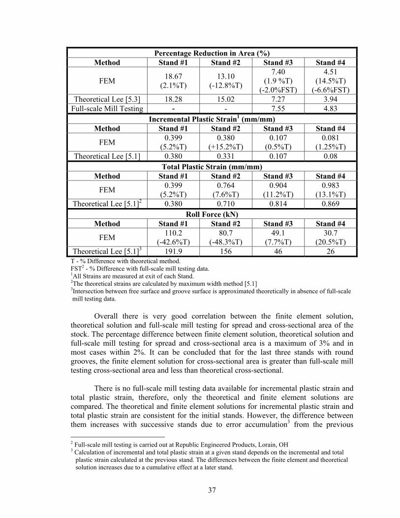
37
Percentage Reduction in Area (%) Method Stand #1 Stand #2 Stand #3 Stand #4
FEM 18.67 (2.1%T)
13.10 (-12.8%T)
7.40 (1.9 %T)
(-2.0%FST)
4.51 (14.5%T)
(-6.6%FST) Theoretical Lee [5.3] 18.28 15.02 7.27 3.94
Full-scale Mill Testing - - 7.55 4.83 Incremental Plastic Strain1 (mm/mm)
Method Stand #1 Stand #2 Stand #3 Stand #4
FEM 0.399 (5.2%T)
0.380 (+15.2%T)
0.107 (0.5%T)
0.081 (1.25%T)
Theoretical Lee [5.1] 0.380 0.331 0.107 0.08 Total Plastic Strain (mm/mm)
Method Stand #1 Stand #2 Stand #3 Stand #4
FEM 0.399 (5.2%T)
0.764 (7.6%T)
0.904 (11.2%T)
0.983 (13.1%T)
Theoretical Lee [5.1]2 0.380 0.710 0.814 0.869 Roll Force (kN)
Method Stand #1 Stand #2 Stand #3 Stand #4
FEM 110.2 (-42.6%T)
80.7 (-48.3%T)
49.1 (7.7%T)
30.7 (20.5%T)
Theoretical Lee [5.1]3 191.9 156 46 26 T - % Difference with theoretical method. FST2 - % Difference with full-scale mill testing data. 1All Strains are measured at exit of each Stand. 2The theoretical strains are calculated by maximum width method [5.1] 3Intersection between free surface and groove surface is approximated theoretically in absence of full-scale mill testing data.
Overall there is very good correlation between the finite element solution, theoretical solution and full-scale mill testing for spread and cross-sectional area of the stock. The percentage difference between finite element solution, theoretical solution and full-scale mill testing for spread and cross-sectional area is a maximum of 3% and in most cases within 2%. It can be concluded that for the last three stands with round grooves, the finite element solution for cross-sectional area is greater than full-scale mill testing cross-sectional area and less than theoretical cross-sectional.
There is no full-scale mill testing data available for incremental plastic strain and
total plastic strain, therefore, only the theoretical and finite element solutions are compared. The theoretical and finite element solutions for incremental plastic strain and total plastic strain are consistent for the initial stands. However, the difference between them increases with successive stands due to error accumulation3 from the previous 2 Full-scale mill testing is carried out at Republic Engineered Products, Lorain, OH 3 Calculation of incremental and total plastic strain at a given stand depends on the incremental and total plastic strain calculated at the previous stand. The differences between the finite element and theoretical solution increases due to a cumulative effect at a later stand.

38
stands. Both the incremental plastic strain and total plastic strain finite element solution is generally greater than the theoretical solution and the maximum percentage difference is 15%. The finite element solution however is more useful since it determines the strain distribution that can be used to find mechanical properties and microstructure.
There is no full-scale mill testing data available for the roll force, therefore, only
the theoretical and finite element solutions are compared. The finite element solution for roll force is less ≈40-50% of the theoretical solution for the first two stands where % reduction is large. This appears very large and is probably due to the fact that the actual model for calculating roll force by Lee [5.2] uses two parameters that are experimentally determined. In absence of experimental data these two parameters were determined theoretically4. For the last two stands, where % reduction is small, the finite element solution for roll force is ≈10-20%greater than the theoretical solution. It was observed that the roll force obtained by the finite element solution is consistent within 10% of a proprietary Morgan [5.11] technique for calculating roll force. The proprietary model employs a combination of empirical techniques and experimental validation.
The results from Stand #4 (last stand) are very important, because geometric roundness and tolerances at the stand exit determines product quality. The results indicate a strong correlation between full-scale mill testing, finite element solution and theoretical solution for spread and cross-sectional area.
4 Maximum contact length (Lmax) and the distance where the roll groove and the deformed stock are separated (Cx) in [5.2] are calculated theoretically in this work.
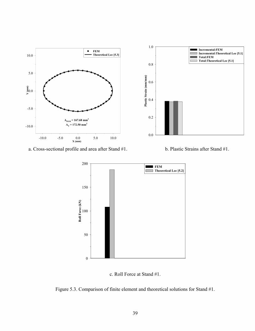
39
X (mm)-10.0 -5.0 0.0 5.0 10.0
Y (m
m)
-10.0
-5.0
0.0
5.0
10.0FEMTheoretical Lee [5.3]
AFEM = 167.68 mm2
AT = 172.50 mm2
Pl
astic
Str
ain
(mm
/mm
)
0.0
0.2
0.4
0.6
0.8
1.0Incremental:FEMIncremental:Theoretical Lee [5.1]Total:FEMTotal:Theoretical Lee [5.1]
a. Cross-sectional profile and area after Stand #1. b. Plastic Strains after Stand #1.
Rol
l For
ce (k
N)
0
50
100
150
200FEMTheoretical Lee [5.2]
c. Roll Force at Stand #1.
Figure 5.3. Comparison of finite element and theoretical solutions for Stand #1.
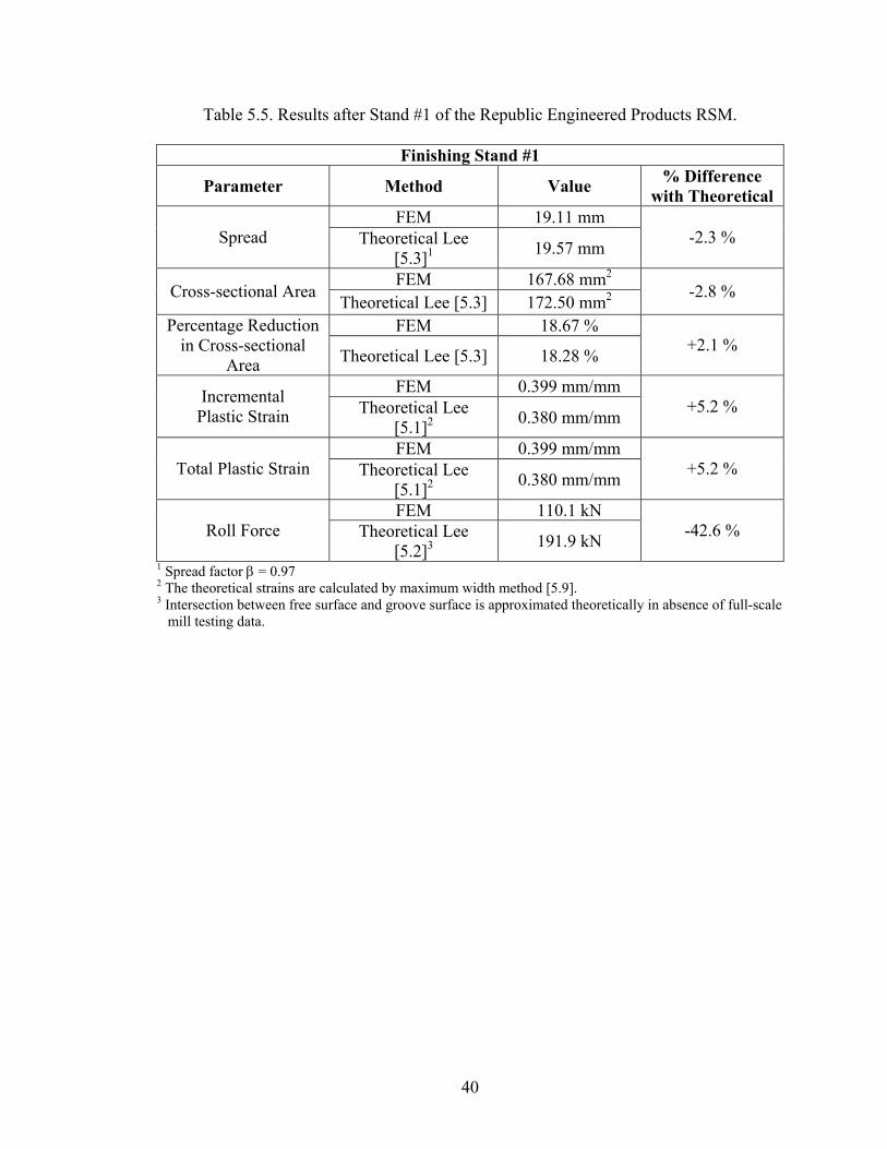
40
Table 5.5. Results after Stand #1 of the Republic Engineered Products RSM.
Finishing Stand #1
Parameter Method Value % Difference with Theoretical
FEM 19.11 mm Spread Theoretical Lee
[5.3]1 19.57 mm -2.3 %
FEM 167.68 mm2
Cross-sectional Area Theoretical Lee [5.3] 172.50 mm2 -2.8 %
FEM 18.67 % Percentage Reduction in Cross-sectional
Area Theoretical Lee [5.3] 18.28 % +2.1 %
FEM 0.399 mm/mm Incremental Plastic Strain Theoretical Lee
[5.1]2 0.380 mm/mm +5.2 %
FEM 0.399 mm/mm Total Plastic Strain Theoretical Lee
[5.1]2 0.380 mm/mm +5.2 %
FEM 110.1 kN Roll Force Theoretical Lee
[5.2]3 191.9 kN -42.6 %
1 Spread factor β = 0.97 2 The theoretical strains are calculated by maximum width method [5.9]. 3 Intersection between free surface and groove surface is approximated theoretically in absence of full-scale mill testing data.

41
X (mm)-10.0 -5.0 0.0 5.0 10.0
Y (m
m)
-10.0
-5.0
0.0
5.0
10.0FEMTheoretical Lee [5.3]
AFEM = 145.72 mm2
AT = 146.60 mm2
AFST = 145.66 mm2
X (mm)
-10.0 -5.0 0.0 5.0 10.0Y
(mm
)
-10.0
-5.0
0.0
5.0
10.0FEMFull-scale Mill Testing
AFEM = 145.72 mm2
AT = 146.60 mm2
AFST = 145.66 mm2
a. Cross-sectional profile and area after Stand #2. b. Cross-sectional profile and area after Stand #1.
Plas
tic S
trai
n (m
m/m
m)
0.0
0.2
0.4
0.6
0.8
1.0Incremental:FEMIncremental:Theoretical Lee [5.1]Total:FEMTotal:Theoretical Lee [5.1]
Rol
l For
ce (k
N)
0
50
100
150
200FEMTheoretical Lee [5.2]
c. Plastic Strains after Stand #2. d. Roll Force at Stand #2.
Figure 5.4. Comparison of finite element and theoretical solutions for Stand #2.

42
Table 5.6. Results after Stand #2 of the Republic Engineered Products RSM.
Finishing Stand #2 % Difference with
Parameter Method Value Theoretical
Full-scale Mill
Testing FEM 13.58 mm
Theoretical Lee [5.3]1 13.70 mm Spread
Full-scale Mill Testing 14.01 mm
-0.88 -3.0
FEM 145.72 mm2
Theoretical Lee [5.3] 146.60 mm2 Cross-sectional Area
Full-scale Mill Testing
145.66 mm2
-0.6 +0.1
FEM 13.10 % Percentage Reduction in Cross-sectional
Area Theoretical Lee [5.3] 15.01 % -12.8 %
FEM 0.38 mm/mm Incremental
Plastic Strain Theoretical Lee [5.1]2
0.33 mm/mm
-15.3
FEM 0.764 mm/mm Total
Plastic Strain Theoretical Lee [5.1]2
0.710 mm/mm
+7.6
FEM 80.7 kN Roll Force Theoretical Lee
[5.2]3 156 kN -48.3
1 Spread factor β = 0.83 2 The theoretical strains are calculated by maximum width method [5.9]. 3 Intersection between free surface and groove surface is approximated theoretically in absence of full-scale mill testing data.

43
X (mm)-10.0 -5.0 0.0 5.0 10.0
Y (m
m)
-10.0
-5.0
0.0
5.0
10.0FEMTheoretical Lee [5.3]
AFEM = 134.92 mm2
AT = 135.94 mm2
AFST = 134.66 mm2
X (mm)-10.0 -5.0 0.0 5.0 10.0
Y (m
m)
-10.0
-5.0
0.0
5.0
10.0FEMFull-scale Mill Testing
AFEM = 134.92 mm2
AT = 135.94 mm2
AFST = 134.66 mm2
a. Cross-sectional profile and area after Stand #3. b. Cross-sectional profile and area after Stand #3.
Plas
tic S
trai
n (m
m/m
m)
0.0
0.2
0.4
0.6
0.8
1.0Incremental:FEMIncremental:Theoretical Lee [5.1]Total:FEMTotal:Theoretical Lee [5.1]
Rol
l For
ce (k
N)
0
50
100
150
200FEMTheoretical Lee [5.2]
c. Plastic Strains after Stand #3. d. Roll Force at Stand #3.
Figure 5.5. Comparison of finite element and theoretical solutions for Stand #3.

44
Table 5.7. Results after Stand #3 of the Republic Engineered Products RSM.
Finishing Stand #3 % Difference with
Parameter Method Value Theoretical
Full-scale Mill Testing
FEM 14.45 mm Theoretical Lee
[5.3]1 14.02 mm Spread Full-scale Mill
Testing 13.98 mm
+3.1 +3.0
FEM 134.92 mm2
Theoretical Lee [5.3] 135.96 mm2 Cross-sectional Area
Full-scale Mill Testing 134.66 mm2
-0.7 +0.2
FEM 7.40 %
Theoretical Lee [5.3] 7.27 % Percentage
Reduction in Cross-sectional Area Full-scale Mill
Testing 7.55 %
+1.8 -2.0
FEM 0.107 mm/mm Incremental
Plastic Strain Theoretical Lee [5.1]2
0.107 mm/mm
+0.5
FEM 0.904 mm/mm Total
Plastic Strain Theoretical Lee [5.1]2
0.813 mm/mm
+11.2
FEM 49 kN Roll Force Theoretical Lee
[5.2]3 46 kN +7.7%
1 Spread factor β = 0.83 2 The theoretical strains are calculated by maximum width method [5.9]. 3 Intersection between free surface and groove surface is approximated theoretically in absence of full-scale mill testing data.

45
X (mm)-10.0 -5.0 0.0 5.0 10.0
Y (m
m)
-10.0
-5.0
0.0
5.0
10.0FEMTheoretical Lee [5.3]
AFEM = 128.84 mm2
AT = 130.59 mm2
AFST = 128.15 mm2
X (mm)-10.0 -5.0 0.0 5.0 10.0
Y (m
m)
-10.0
-5.0
0.0
5.0
10.0FEMFull-scale Mill Testing
AFEM = 128.84 mm2
AT = 130.59 mm2
AFST = 128.15 mm2
a. Cross-sectional profile and area after Stand #4. b. Cross-sectional profile and area after Stand #4.
Plas
tic S
trai
n (m
m/m
m)
0.0
0.2
0.4
0.6
0.8
1.0Incremental:FEMIncremental:Theoretical Lee [5.1]Total:FEMTotal:Theoretical Lee [5.1]
Rol
l For
ce (k
N)
0
50
100
150
200FEMTheoretical Lee [5.2]
c. Plastic Strains after Stand #4. d. Roll Force at Stand #4.
Figure 5.6. Comparison of finite element and theoretical solutions for Stand #4.
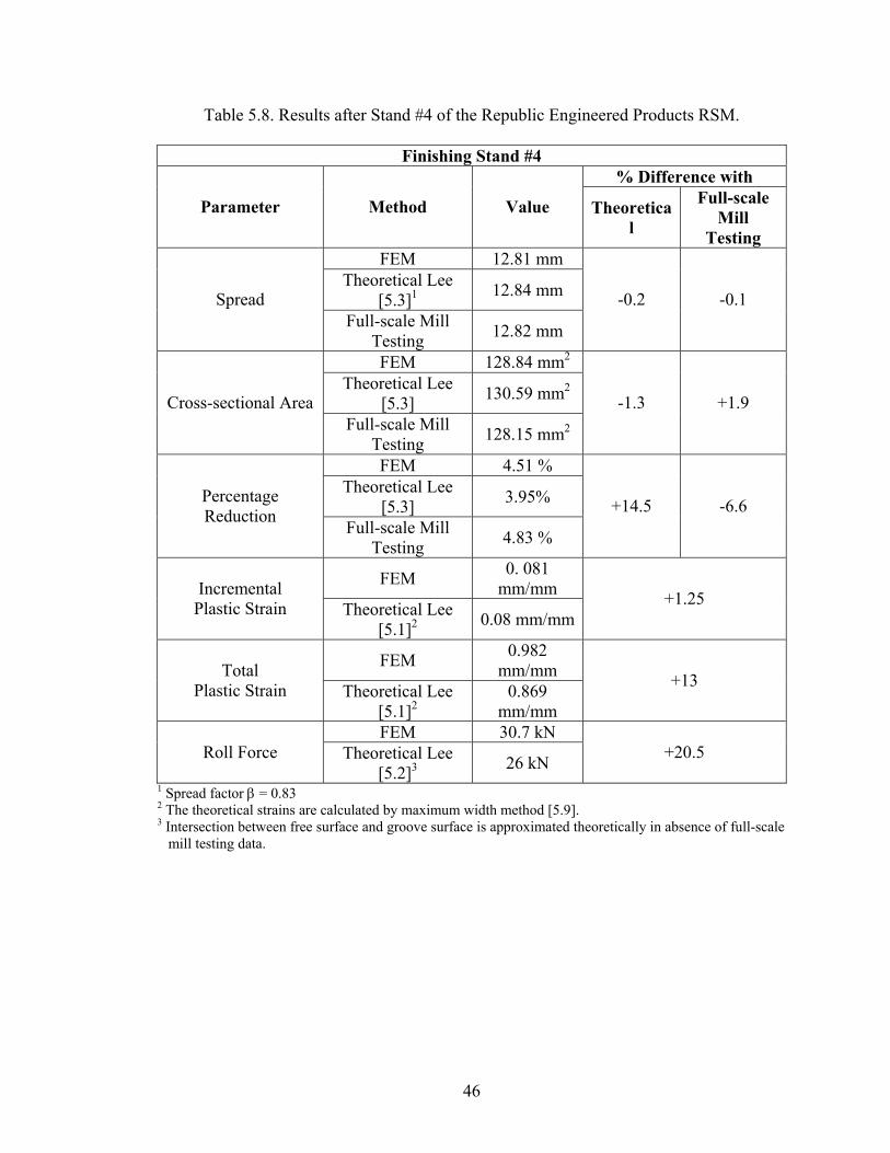
46
Table 5.8. Results after Stand #4 of the Republic Engineered Products RSM.
Finishing Stand #4 % Difference with
Parameter Method Value Theoretical
Full-scale Mill
Testing FEM 12.81 mm
Theoretical Lee [5.3]1 12.84 mm Spread
Full-scale Mill Testing 12.82 mm
-0.2 -0.1
FEM 128.84 mm2
Theoretical Lee [5.3] 130.59 mm2 Cross-sectional Area
Full-scale Mill Testing 128.15 mm2
-1.3 +1.9
FEM 4.51 %
Theoretical Lee [5.3] 3.95% Percentage
Reduction Full-scale Mill Testing 4.83 %
+14.5 -6.6
FEM 0. 081 mm/mm Incremental
Plastic Strain Theoretical Lee [5.1]2 0.08 mm/mm
+1.25
FEM 0.982 mm/mm Total
Plastic Strain Theoretical Lee [5.1]2
0.869 mm/mm
+13
FEM 30.7 kN Roll Force Theoretical Lee
[5.2]3 26 kN +20.5
1 Spread factor β = 0.83 2 The theoretical strains are calculated by maximum width method [5.9]. 3 Intersection between free surface and groove surface is approximated theoretically in absence of full-scale mill testing data.

47
a. Arrangement of rolling stand in multi-stand rolling (Repeated from Figure 5.2)
b. Stand #1. c. Stand #2.
d. Stand #3. e. Stand #4.
Figure 5.7. Finite element solution of total plastic strain variation in stock at each stand.

48
5.2.5. Are Customer Requirements Satisfied?
The geometric requirements of the finished rod are stated in Table 5.10 and were provided by the U.S. automotive supplier and are based on ASTM standards [5.8]. Tables 5.8 and 5.9 demonstrate good correlation of the finite element model with the design objective to produce rod with a circular cross section in the mill on-line. Note that the theoretical model does give a very good geometric prediction in this case. However, the theoretical model cannot consider steel grade and coupling effects. Furthermore, this type of model cannot predict the distribution of microstructural and mechanical properties throughout the rod. This is very important where a steel mill must satisfy customer requirements for a uniform distribution of mechanical and microstructural properties through out the rod. Although the finite results do not satisfy customer requirements fully in this case, it is expected that the predictions will improve as the finite element model includes all the coupling effects shown in Figure 2.3. This work demonstrates the potential for development of the proposed coupled thermo-deformation-microstructural simulation model shown in Figure 2.2.
Table 5.9. Comparison of full-scale mill testing, FEM and theoretical geometric results at
exit of fourth finishing stand in Republic Engineered Products, Lorain, OH.
PARAMETER FULL-SCALE MILL TESTING2 FEM3 THEORETICAL
[5.1-5.3]
Maximum Diameter1 12.82 mm 12.81 mm (-0.1%)
12.84 mm (+0.30%)
Minimum Diameter 12.75 mm 12.71 mm (-0.34%)
12.79 mm (+0.31%)
Cross-sectional Area 128.15 mm2 127.97 mm2 (-0.15%)
128.75 mm2 (+0.47%)
1Provided by Republic Engineered Products Ohio industrial partner. 2The quantity in parentheses represent the percentage difference between the parameter shown in the column and full-scale mill testing. 3The quantity in parentheses represents the percentage difference between the parameter shown in the column and the full-scale mill testing
Table 5.10. Geometry customer requirements and a comparison with full-scale mill testing, FEM and theoretical model.
ASTM REQUIREMENTS FULL-SCALE MILL TESTING3 FEM THEORETICAL
[5.1-5.3] Roundness1 0.08 mm 0.06 mm 0.1 mm 0.12 mm [4-6] Tolerance2 + 0.08 mm + 0.07 mm + 0.06 mm +0.04 mm [4-6]
1Roundness is the difference between maximum diameter and minimum diameter. 2Tolerance is the allowable difference in diameter between what a customer orders and what the steel mill delivers. 3 Provided by Republic Engineered Products Ohio industrial partner.
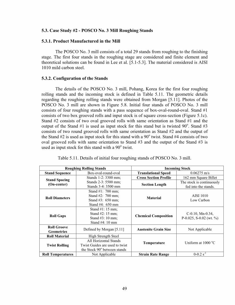
49
5.3. Case Study #2 - POSCO No. 3 Mill Roughing Stands 5.3.1. Product Manufactured in the Mill The POSCO No. 3 mill consists of a total 29 stands from roughing to the finishing stage. The first four stands in the roughing stage are considered and finite element and theoretical solutions can be found in Lee et al. [5.1-5.3]. The material considered is AISI 1010 mild carbon steel. 5.3.2. Configuration of the Stands
The details of the POSCO No. 3 mill, Pohang, Korea for the first four roughing rolling stands and the incoming stock is defined in Table 5.11. The geometric details regarding the roughing rolling stands were obtained from Morgan [5.11]. Photos of the POSCO No. 3 mill are shown in Figure 5.8. Initial four stands of POSCO No. 3 mill consists of four roughing stands with a pass sequence of box-oval-round-oval. Stand #1 consists of two box grooved rolls and input stock is of square cross-section (Figure 5.1c). Stand #2 consists of two oval grooved rolls with same orientation as Stand #1 and the output of the Stand #1 is used as input stock for this stand but is twisted 90o. Stand #3 consists of two round grooved rolls with same orientation as Stand #2 and the output of the Stand #2 is used as input stock for this stand with a 90o twist. Stand #4 consists of two oval grooved rolls with same orientation to Stand #3 and the output of the Stand #3 is used as input stock for this stand with a 90o twist.
Table 5.11. Details of initial four roughing stands of POSCO No. 3 mill.
Roughing Rolling Stands Incoming Stock
Stand Sequence Box-oval-round-oval Translational Speed 0.06275 m/s Cross Section Profile 162 mm Square Billet Stand Spacing
(On-center)
Stands 1-2: 3300 mm; Stands 2-3: 5500 mm; Stands 3-4: 3500 mm Section Length The stock is continuously
fed into the stands.
Roll Diameters
Stand #1: 700 mm; Stand #2: 700 mm; Stand #3: 650 mm; Stand #4: 650 mm
Material AISI 1010 Low Carbon
Roll Gaps
Stand #1: 15 mm; Stand #2: 15 mm; Stand #3: 10 mm; Stand #4: 10 mm
Chemical Composition C-0.10, Mn-0.34, P-0.025, S-0.02 (wt. %)
Roll Groove Geometries Defined by Morgan [5.11] Austenite Grain Size Not Applicable
Roll Material High Strength Steel
Twist Rolling All Horizontal Stands
Twist Guides are used to twist the Stock 90o between stands
Temperature Uniform at 1000 oC
Roll Temperatures Not Applicable Strain Rate Range 0-0.2 s-1

50
Rotational Speed of Rolls
Stand #1: 2.8 rpm; Stand #2: 3.5 rpm; Stand #3: 5.7 rpm; Stand #4: 7.1 rpm
Specific Heat 475 J/Kg/K [5.7]
Roll/Stock Friction Friction due to Contact between High Strength Steel Roll and AISI 1045 Stock Surface with Water Present between as Coolant.
1Linear dimensions at room temperature is corrected by +1% due to thermal expansion from room temperature to 1000 oC (Commonly used by Morgan Construction Company [5.11])
a. Mill Overall View
b. Stand Configuration
Figure 5.8. Roughing stands POSCO No. 3 mill.
5.3.3. How is the Problem Modeled using FEM?
The commercial finite element code ABAQUS/Explicit [5.10] was used in this
work. Table 5.12 states the assumptions, solution techniques and other modeling parameters used in the finite element simulation of the POSCO No. 3 mill. Each item

51
shown in Table 5.12 is discussed in-depth in Appendix E. For this study, the POSCO No. 3 mill was analyzed as a complete assembly i.e., four stands. A finite element pre and post-processor program is written using Python script and Java (Appendix A & B) to analyze the results of the finite element solution and verify it with theoretical results.
Table 5.12. Details of ABAQUS/Explicit finite element model for the POSCO No. 3 mill
roughing stands.
Mesh Domain Lagrangian Time Dependence Transient
Time Integration Explicit, Dynamics, Adiabatic.
Optimal time step is decided automatically by ABAQUS
Dimensionality Three-Dimensional Mass Scaling None
Adaptive Meshing Lagrangian Analysis: No
Formulation
Hourglass Artificial Stiffness
Element Type Linear Hexahedral Brick (C3D8R), Deformable, Reduced Integration
Mesh Characteristics #of Nodes: 4753
#of Elements: 3456 #of DOF: 14307 (including Lagrange Multipliers)
Material Homogeneous and Isotropic Length 2.5 m1
Rate Dependence Yes Spring Back Calculation No
Plasticity Law Shida2 [5.4] Hardening Rate Isotropic
% Plastic Deformation Energy Converted to Heat 0.90 [5.9]
Stock
Initial Conditions Initial Velocity of the Stock; Initial Temperature of the Stock
Material Rigid Finite Element Characterization Analytic Rigid Surface Roll
Boundary Conditions Rotational Speed of Rolls in Table 5.11
Contact Condition Tangential: Penalty; Normal: Hard
Friction Model Coulomb (µ=0.3) Stock / Roll
Interface Heat Transfer Effects Not Applicable
Material Rigid Pin support at Roll
Model Spacing (On-center)1 Stands 1-2: 850 mm; Stands 2-3: 900 mm; Stands 3-4: 900 mm Stand
Orientation3
Stand #1: Vertical; Stand #2: Horizontal;
Stand #3: Vertical; Stand #4: Horizontal
1The section length of the stock is 1.0 m in the finite element model to reduce the number of degrees of freedom in the model. Inter-stand distances are also minimized for the same reason. 2Appropriate models are used based on expected strain rate range in Table 5.2. 3Stand orientation for the finite element model was assumed oriented vertically and horizontally for simplicity in model creation
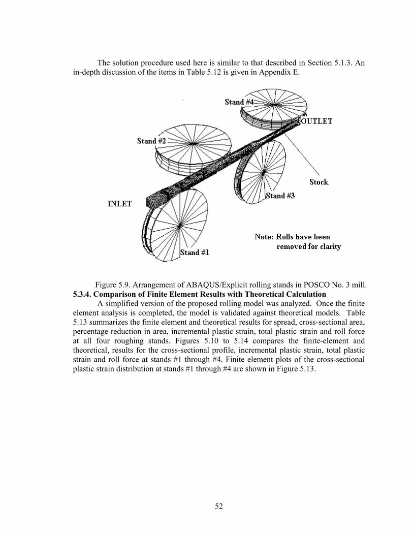
52
The solution procedure used here is similar to that described in Section 5.1.3. An
in-depth discussion of the items in Table 5.12 is given in Appendix E.
Figure 5.9. Arrangement of ABAQUS/Explicit rolling stands in POSCO No. 3 mill.
5.3.4. Comparison of Finite Element Results with Theoretical Calculation A simplified version of the proposed rolling model was analyzed. Once the finite
element analysis is completed, the model is validated against theoretical models. Table 5.13 summarizes the finite element and theoretical results for spread, cross-sectional area, percentage reduction in area, incremental plastic strain, total plastic strain and roll force at all four roughing stands. Figures 5.10 to 5.14 compares the finite-element and theoretical, results for the cross-sectional profile, incremental plastic strain, total plastic strain and roll force at stands #1 through #4. Finite element plots of the cross-sectional plastic strain distribution at stands #1 through #4 are shown in Figure 5.13.

53
Table 5.13. Comparison of full-scale mill testing, FEM and theoretical geometric results at each roughing stand for POSCO No. 3 mill.
Formulation Type Lagrangian Constitutive Law Shida [F.3] Number of Nodes 3456
Number of Elements Freedom in the problem 4753
Characteristics of Finite Element
Model Number of Degrees of Freedom
(Including Lagrange multipliers) 14307
Spread (mm) Method Stand #1 Stand #2 Stand #3 Stand #4
FEM 182.58 (-2.7%T)
196.36 (4.5%T)
114.68 (-3.8%T)
146.84 (-3.5%T)
Theoretical Lee [5.3] 187.65 187.97 119.27 152.18 Cross-sectional Area (mm2)
Method Stand #1 Stand #2 Stand #3 Stand #4
FEM 20352.26 (-2.3%T)
14546.11 (-0.4%T)
10825.26 (-2.8%T)
8119.19 (-2.5%T)
Theoretical Lee [5.3] 20828.64 14501.47 11142.66 8328.73 Percentage Reduction in Area (%)
Method Stand #1 Stand #2 Stand #3 Stand #4
FEM 22.45 (8.8%T)
29.05 (-4.4%T)
25.04 (8.1%T)
24.99 (-1.0%T)
Theoretical Lee [5.3] 20.63 30.38 23.16 25.25 Incremental Plastic Strain1 (mm/mm)
Method Stand #1 Stand #2 Stand #3 Stand #4
FEM 0.414 (8.7%T)
0.777 (-5.4%T)
0.507 (-3%T)
0.487 (-10.8%T)
Theoretical Lee [5.1] 0.381 0.821 0.523 0.540 Total Plastic Strain (mm/mm)
Method Stand #1 Stand #2 Stand #3 Stand #4
FEM 0.414 (8.7%T)
1.293 (8.0%T)
1.795 (4.34%T)
2.124 (-6.3%T)
Theoretical Lee [5.1]2 0.381 1.197 1.720 2.266 Roll Force (kN)
Method Stand #1 Stand #2 Stand #3 Stand #4
FEM 2406.03 (-29.1%T)
2673.21 (-34.3%T)
2003.48 (-37.3%T)
1692.73 (-46.8%T)
Theoretical Lee [5.1]3 3394 4069 3196 3182 T - % Difference with theoretical method. 1All Strains are measured at exit of each Stand. 2The theoretical strains are calculated by maximum width method [5.1] 3Intersection between free surface and groove surface is approximated theoretically in absence of full-scale mill testing data.
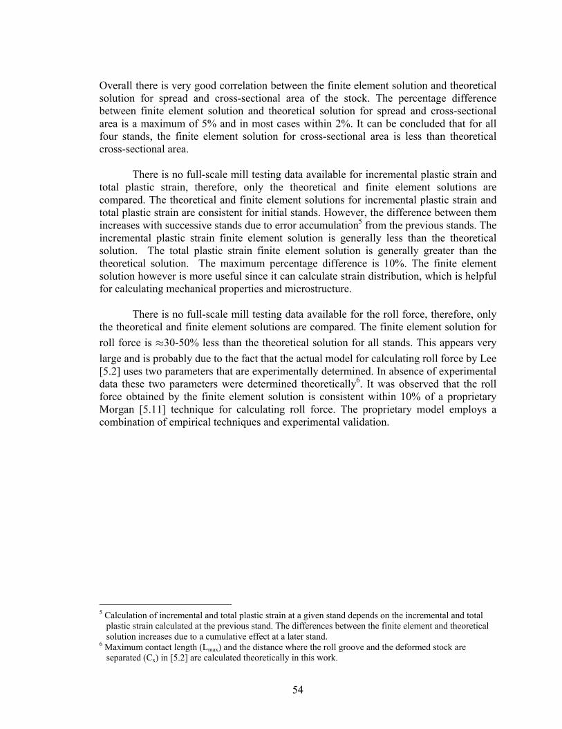
54
Overall there is very good correlation between the finite element solution and theoretical solution for spread and cross-sectional area of the stock. The percentage difference between finite element solution and theoretical solution for spread and cross-sectional area is a maximum of 5% and in most cases within 2%. It can be concluded that for all four stands, the finite element solution for cross-sectional area is less than theoretical cross-sectional area.
There is no full-scale mill testing data available for incremental plastic strain and
total plastic strain, therefore, only the theoretical and finite element solutions are compared. The theoretical and finite element solutions for incremental plastic strain and total plastic strain are consistent for initial stands. However, the difference between them increases with successive stands due to error accumulation5 from the previous stands. The incremental plastic strain finite element solution is generally less than the theoretical solution. The total plastic strain finite element solution is generally greater than the theoretical solution. The maximum percentage difference is 10%. The finite element solution however is more useful since it can calculate strain distribution, which is helpful for calculating mechanical properties and microstructure.
There is no full-scale mill testing data available for the roll force, therefore, only
the theoretical and finite element solutions are compared. The finite element solution for roll force is ≈30-50% less than the theoretical solution for all stands. This appears very large and is probably due to the fact that the actual model for calculating roll force by Lee [5.2] uses two parameters that are experimentally determined. In absence of experimental data these two parameters were determined theoretically6. It was observed that the roll force obtained by the finite element solution is consistent within 10% of a proprietary Morgan [5.11] technique for calculating roll force. The proprietary model employs a combination of empirical techniques and experimental validation.
5 Calculation of incremental and total plastic strain at a given stand depends on the incremental and total plastic strain calculated at the previous stand. The differences between the finite element and theoretical solution increases due to a cumulative effect at a later stand. 6 Maximum contact length (Lmax) and the distance where the roll groove and the deformed stock are separated (Cx) in [5.2] are calculated theoretically in this work.
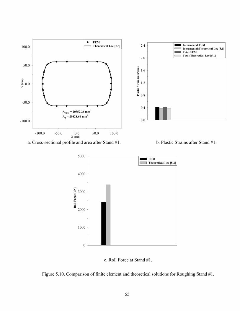
55
X (mm)-100.0 -50.0 0.0 50.0 100.0
Y (m
m)
-100.0
-50.0
0.0
50.0
100.0FEMTheoretical Lee [5.3]
AFEM = 20352.26 mm2
AT = 20828.64 mm2
Pl
astic
Str
ain
(mm
/mm
)
0.0
0.4
0.8
1.2
1.6
2.0
2.4 Incremental:FEMIncremental:Theoretical Lee [5.1]Total:FEMTotal:Theoretical Lee [5.1]
a. Cross-sectional profile and area after Stand #1. b. Plastic Strains after Stand #1.
Rol
l For
ce (k
N)
0
1000
2000
3000
4000
5000FEMTheoretical Lee [5.2]
c. Roll Force at Stand #1.
Figure 5.10. Comparison of finite element and theoretical solutions for Roughing Stand #1.

56
Table 5.14. Results after roughing Stand #1 of the POSCO No. 3 mill.
Roughing Stand #1
Parameter Method Value % Difference with Theoretical
FEM 182.58 mm Spread Theoretical Lee
[5.3]1 187.65 mm -2.7
FEM 20352.26 mm2
Cross-sectional Area Theoretical Lee [5.3] 20828.64 mm2 -2.3
FEM 22.45 % Percentage Reduction in Cross-sectional
Area Theoretical Lee [5.3] 20.63 % +8.8
FEM 0.414 mm/mm Incremental Plastic Strain Theoretical Lee
[5.1]2 0.381 mm/mm +8.7
FEM 0.414 mm/mm Total Plastic Strain Theoretical Lee
[5.1]2 0.381 mm/mm +8.7
FEM 2406.03 Roll Force Theoretical Lee
[5.2]3 3394 -29.1
1 Spread factor β = 0.83 2 The theoretical strains are calculated by maximum width method [5.9]. 3 Intersection between free surface and groove surface is approximated theoretically in absence of full-scale mill testing data.

57
X (mm)-100.0 -50.0 0.0 50.0 100.0
Y (m
m)
-100.0
-50.0
0.0
50.0
100.0
FEMTheoretical Lee [5.3]
AFEM = 14440.42 mm2
AT = 14501.47 mm2
Pl
astic
Str
ain
(mm
/mm
)
0.0
0.4
0.8
1.2
1.6
2.0
2.4 Incremental:FEMIncremental:Theoretical Lee [5.1]Total:FEMTotal:Theoretical Lee [5.1]
a. Cross-sectional profile and area after Stand #2. b. Plastic Strains after Stand #2.
Rol
l For
ce (k
N)
0
1000
2000
3000
4000
5000FEMTheoretical Lee [5.2]
c. Roll Force at Stand #2.
Figure 5.11. Comparison of finite element and theoretical solutions for Roughing Stand #2.

58
Table 5.15. Results after roughing Stand #2 of the POSCO No. 3 mill.
Roughing Stand #2
Parameter Method Value % Difference with Theoretical
FEM 196.36 mm Spread Theoretical Lee [5.3]1 187.97 mm 4.5
FEM 14440.42 mm2
Cross-sectional Area Theoretical Lee [5.3] 14501.47 mm2 -0.4
FEM 29.04 % Percentage Reduction in Cross-sectional
Area Theoretical Lee [5.3] 30.38 % -4.4
FEM 0.777 mm/mm Incremental Plastic Strain Theoretical Lee [5.1]2 0.821 mm/mm -5.4
FEM 1.293 mm/mm Total Plastic Strain Theoretical Lee [5.1]2 1.197 mm/mm 8.0
FEM 2673.21 Roll Force Theoretical Lee [5.2]3 4069 -34.3 1 Spread factor β = 1.00 2 The theoretical strains are calculated by maximum width method [5.9]. 3 Intersection between free surface and groove surface is approximated theoretically in absence of full-scale mill testing data.

59
X (mm)-100.0 -50.0 0.0 50.0 100.0
Y (m
m)
-100.0
-50.0
0.0
50.0
100.0FEMTheoretical Lee [5.3]
AFEM = 10825.26 mm2
AT = 11142.66 mm2
Pl
astic
Str
ain
(mm
/mm
)
0.0
0.4
0.8
1.2
1.6
2.0
2.4 Incremental:FEMIncremental:Theoretical Lee [5.1]Total:FEMTotal:Theoretical Lee [5.1]
a. Cross-sectional profile and area after Stand #3. b. Plastic Strains after Stand #3.
Rol
l For
ce (k
N)
0
1000
2000
3000
4000
5000FEMTheoretical Lee [5.2]
c. Roll Force at Stand #3.
Figure 5.12. Comparison of finite element and theoretical solutions for Roughing Stand #3.

60
Table 5.16. Results after roughing Stand #3 of the POSCO No. 3 mill.
Roughing Stand #3
Parameter Method Value % Difference with Theoretical
FEM 114.68 mm Spread Theoretical Lee [5.3]1 119.27 mm
-3.8
FEM 10825.26 mm2
Cross-sectional Area Theoretical Lee [5.3] 11142.66 mm2
-2.9
FEM 25.03 % Percentage Reduction in Cross-
sectional Area Theoretical Lee [5.3] 23.96 % 8.1
FEM 0.507 mm/mm Incremental Plastic Strain Theoretical Lee [5.1]2 0.523 mm/mm -3.1
FEM 1.795 mm/mm Total Plastic Strain Theoretical Lee [5.1]2 1.720 mm/mm +4.3
FEM 2003.48 Roll Force Theoretical Lee [5.2]3 3196 -37.3 1 Spread factor β = 0.83 2 The theoretical strains are calculated by maximum width method [5.9]. 3 Intersection between free surface and groove surface is approximated theoretically in absence of full-scale mill testing data.

61
X (mm)-100.0 -50.0 0.0 50.0 100.0
Y (m
m)
-100.0
-50.0
0.0
50.0
100.0FEMTheoretical Lee [5.3]
AFEM = 8119.19 mm2
AT = 8328.73 mm2
Plas
tic S
trai
n (m
m/m
m)
0.0
0.4
0.8
1.2
1.6
2.0
2.4 Incremental:FEMIncremental:Theoretical Lee [5.1]Total:FEMTotal:Theoretical Lee [5.1]
a. Cross-sectional profile and area after Stand #4. b. Plastic Strains after Stand #4.
Rol
l For
ce (k
N)
0
1000
2000
3000
4000
5000FEMTheoretical Lee [5.2]
c. Roll Force at Stand #4.
Figure 5.13. Comparison of finite element and theoretical solutions for Roughing Stand #4.

62
Table 5.17. Results after roughing Stand #4 of the POSCO No. 3 mill.
Roughing Stand #4
Parameter Method Value % Difference
with Theoretical
FEM 146.84 mm Spread Theoretical Lee [5.3] 1 152.18 mm -3.5
FEM 8119.19 mm2
Cross-sectional Area Theoretical Lee [5.3] 8328.73 mm2 -2.5
FEM 24.99 % Percentage Reduction Theoretical Lee [5.3] 25.25 % -1.0
FEM 0.487 mm/mm Incremental Plastic Strain Theoretical Lee [5.1] 2 0.540 mm/mm -10.8
FEM 2.124 mm/mm Total Plastic Strain Theoretical Lee [5.1] 2 2.266 mm/mm -6.3
FEM 1692.73 Roll Force Theoretical Lee [5.2] 3 3182 -46.8 1 Spread factor β = 0.97 2 The theoretical strains are calculated by maximum width method [5.9]. 3 Intersection between free surface and groove surface is approximated theoretically in absence of full-scale mill testing data.
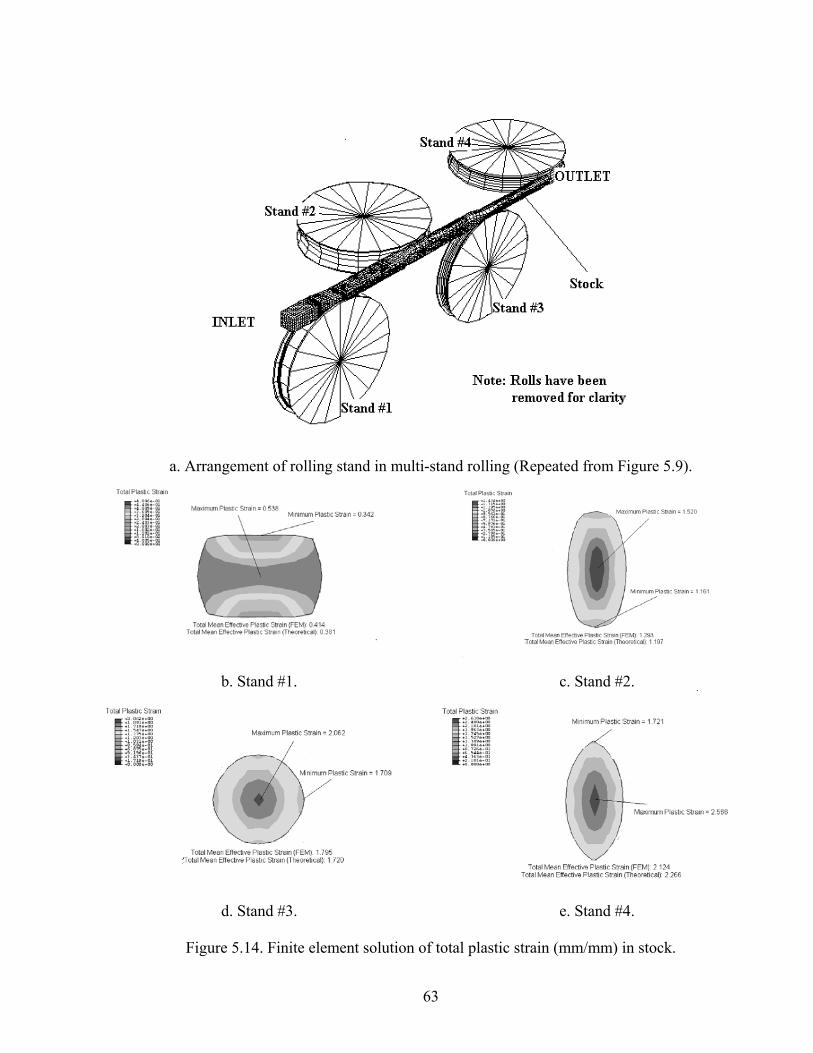
63
a. Arrangement of rolling stand in multi-stand rolling (Repeated from Figure 5.9).
b. Stand #1. c. Stand #2.
d. Stand #3. e. Stand #4.
Figure 5.14. Finite element solution of total plastic strain (mm/mm) in stock.
64
6. Conclusion A Java pre- and post-processing graphical user-oriented interface has been developed to aid a mill engineer with little or no finite element experience throughout the analysis process of the finishing rolling stands. This work validated the application of ABAQUS/Explicit Lagrangian solution modeling technique to simulate both high speed finishing stand (Republic Engineered Products RSM mill) and slow speed roughing stand (First four stands of POSCO No. 3 mill) rolling. It has been demonstrated that the finite element modeling techniques used in this work successfully predict geometrical shape (spread, cross-sectional area and shape of the stock), incremental plastic effective strain and total plastic effective strain for a wide range of rolling speed (0.05-0.2 m/s and 19-30m/s), strain rate (0.1-0.2s-1 and 350-500s-1) and different stock materials (AISI 1010 and AISI 1045 steel). In this work various strain rate and temperature dependent plasticity models were used. It has been found that parameters like geometrical shape (spread, cross-sectional area and shape of the stock) vary negligibly with the employment of these models instead of using a simple plastic strain model considered in previous work [6.1]. However the roll force varies significantly with different plasticity model. Though it has been demonstrated that roll force data doesn’t compare well with the available theoretical model it has been found that the roll force data obtained from the finite element analysis is consistent to results obtained by a proprietary Morgan technique. The Morgan roll force model employs a combination of empirical techniques that have been experimentally validated. In this work a thermo-mechanically coupled finite element model has been employed. It has been found that parameters like geometrical shape vary negligibly with the employment of the thermo-mechanically coupled finite element model instead of using a thermally uncoupled model used in previous work [6.1]. The ability to accurately predict formed geometrical shape (spread, cross-sectional area and shape of the stock), incremental plastic effective strain and total plastic effective strain, based on process parameters, is very encouraging. The simulation approach described herein can still be used to evaluate roller groove-shapes, root diameters, and tolerances of the roll shape and positions within a stand. The finite element solution for the last stand of Republic Engineered Products RSM mill lies within the ASTM [6.2] roundness and tolerance requirements. This capability is presently valuable for the purpose of design comparisons.

65
7. Future Work Initial work done on the finite element modeling and theoretical solution of
Republic Engineered Products finishing stands and POSCO No. 3 mill roughing stands has yielded important information and insight on how to carry out future work for full-scale rolling mill simulation and the best way of achieving it. The major thrust of any future work should be in evaluating the complete range of parameters important to designers and manufacturers of rolling mills, both theoretically and by the finite element method. Furthermore, improving both theoretical and finite element solutions to meet the customer requirements of tolerance in various parameters of the output rolled product. The complete research and developmental work required to be done is listed briefly in Figure 2.2. In this chapter we will discuss some aspects of future work. 7.1. Theoretical Thermo-Mechanical Model 7.1.1. Theoretical Calculation of Stock Temperature during the Rolling Process
Temperature of stock during the rolling process varies from stand to stand due to following mechanisms:
• Heat Generation Due to Plastic Deformation. Heat is generated in the stock when plastic deformation of the stock takes place as a part of the energy expended to deform the stock is converted into heat.
• Friction Between Stock and Rolls. Some part of the work due to friction is converted into heat and then some part of this heat is transferred to the stock.
• Heat Transfer. Heat transfer mechanisms include conduction (between roll and stock), convection (between stock and environment), and radiation (between stock and environment).
Several researchers have attempted to calculate stock temperature distribution in multi stand rolling using different assumptions. They include Lee et al. [7.1] and Serajzadeh et al. [7.2].
Lee et al. [7.1] in 2002 applied the equivalent circle approximation to the temperature distribution problem in the multi-stand rolling problem and developed a one-dimensional axisymmetric differential equation of the temperature distribution, which was then solved by finite difference method using the boundary condition of Braun-Angott et al. [7.3] and Carnahan [7.4]. The heat transfer equation is given by the following
,pT Tk q C
r r tρ∂ ∂ ∂ + = ∂ ∂ ∂
(7.1a)
p
qC
σεχρβ
= (7.1b)

66
where, T is the stock temperature, t is time, k is conductivity, ρ is stock density, χ is fraction of plastic deformation work converted in to heat in stock, β is mechanical equivalent of heat, Cp is specific heat of stock, σ is stock flow stress, ε is stock strain rate and q is heat generation rate of stock. This model only accounts for conduction in the stock.
Serajzadeh et al. [7.2] in 2002 considered a more general case where the heat transfer in the peripheral direction is negligible. The governing partial differential equation is given as follows
1p
T T Tk k Cr r r z z t
ρ∂ ∂ ∂ ∂ ∂ + = ∂ ∂ ∂ ∂ ∂ (7.2a)
with the following initial and boundary conditions ( ) 0, , 0T r z t T= = (7.2b)
( )( )*r
r R
Tk h t T Tr =
∂ − = − ∂ (7.2c)
*
0r r
Tkr =
∂ − = ∂ (7.2d)
where T, t, r, ρ, k and Cp are temperature, time, distance from roll axis, density, heat conductivity and specific heat of the stock, respectively. Also, Tr is roll surface temperature, h* is convective coefficient between roll and stock and r* is the radius below which heat transfer can be neglected. 7.1.2. Microstructure Evolution of Stock During the Rolling Process
An important customer requirement that has to be determined is microstructure evolution of the stock during rolling since mechanical properties of the output products depend on microstructure. According to mainstream literature microstructure depends on the following parameters:
• Temperature Distribution in the Stock • Strain and Strain Rate in the Stock • Inter-Stand time • Cooling Mechanism of the Stock
Several researchers have proposed different models to calculate the microstructure evolution of the stock during multi-stand rolling. Prominent among them are Sellars [7.5], Yanagimoto et al. [7.6] and Farrugia et al. [7.7].

67
7.2. Finite Element Modeling 7.2.1. Calculation of Output Parameters for Rolling Mill by post processing FEM
Output Results
The commercial finite element software ABAQUS is used to solve the rolling mill simulation problem where output is determined in terms of general mechanical variables that include displacement, strain, stress energy, etc. These results have to be post processed using an in-house code for calculating parameters important to designers and manufacturers of rolling mills. Although some parameters such as spread, plastic strain, cross sectional area of the stock after each stand have been calculated in this work by post-processing the finite element results the complete range of parameters including roll torque and the power requirements have to be calculated in this way. 7.2.2. Improvements to the Finite Element Model
The finite element model currently used in this work is based on Lagrangian and transient Arbitrary Eulerian-Lagrangian (ALE) formulations. Though these models yield results that are generally in agreement with the experimental geometrical data, these methods are computationally expensive. Another way of modeling the problem is the steady-state ALE formulation. This method requires an initial guess of the three-dimensional stock geometry at each stand as well as between stands. The closer the initial geometry is, to the actual geometry, the faster the solution time. A theoretical three-dimensional geometrical solution for the stock, in multi-stand rolling has been developed by Bayoumi et al. [7.8]. If used as an initial geometric guess in the steady-state ALE formulation, this approximate three-dimensional geometrical solution can be used to reduce solution time. If this approach is successful the flowchart of the model in Figure 2.3 would become Figure 7.1 the step (box) second from the top has been added. 7.3. Improvement of Theoretical-Empirical Model Based on Numerical Experiments
While it is known that solution to the multi-stand rolling problem is influenced by numerous factors such as stock velocity and stand spacing most theoretical-empirical models neglect most factors for simplicity. For example, the most recent theoretical-empirical model by Lee et al. [7.9] to calculate spread assumes that spread depends only on stock and roll geometry. This is because almost all past models depend on various experimentally determined coefficients, which are expensive enough to study all the parameters affecting the ultimate result. A well-established and validated finite element model in contrast can be used in place of experiments. Numerical experiments cost only a fraction of actual experimentation and can be used to study effect of the above-discussed parameters. Results of these experiments can then be included to generalize theoretical-empirical models. This approach is very feasible due to rapidly decreasing computing costs.

68
Figure 7.1. Proposed flowchart if steady-state finite element modeling is successful.
Modify Process
Modify Model
IN P U T T O F E M F IN ISH IN G R O L L IN G M O D E L F inishing R olling Stands Incom ing Stock
Pass S equence T ransla tional S peed S tand Spacings Section Profile
S tand S tiffnesses S ection L ength R oll M ateria l M ateria l
R oll D ia m eters C hem ical C omposition R oll G aps Austenite G rain S ize
R oll G rove G eom etries T emp erature N o-tw ist R olling S tress-stra in-S tra in R ate D ata R oll T emp erature
R ota tional S peed of R olls R oll/S tock Friction
H eat Flow H eating Coo ling
V ariat ion o f T hermo-physica l
Properties
T H R E E-D IM E N SIO N A L F EM R O L L IN G M O D EL D efo rm ation
Ro lling Fo rce and T orque Flow Stress
S train and Strain Rate Contact and Fr ict ion
T emperature Chem ical Co mposit io n
Phases P resent
M icrostructure Chem ical Co mpo sit io nT emperature vs T im e
% D eformat io n Initia l A usten ite Grain Size
Coo ling Co nd it io ns M icro M odel M icro M odel
M acro M odel
O U T PU T FR O M FEM R O L L ING M O D EL G eom etry M echanical P roperties M icrostructure
Sectio n P ro file Y ie ld S trength G rain S ize Roundness U lt im ate T ensile S trength G rain S ize D istribution T o lerance % Reductio n in Area Phase Compo sit io n
H ardness Phase D istribut ion
N ot V alidated F U LL-SC A LE
M IL L T ESTIN G & T H EO R ETIC A L/
E M PIR IC A L M O D EL
C U ST O M E R R E Q U IR EM E N T S
G eom etr y M ech an ical Properties
M icrostructure
M A N U FA C T U RE P R O D U C T IN M IL L O N -L IN E
Satisfied
N ot Satisfied
Initial Three-dimensional Geometrical Solution
69
References 1.1. Steel Industry Technology Roadmap, American Iron and Steel Institute,
Washington, DC, February 1998, http://www.steel.org/mt/roadmap/ roadmap.htm.
1.2. Marcus, P.F. and Kirsis, K.M., “Steel in 2001: Constraints Unparalleled. Opportunities Unmatched,” Steel Success Strategies XVI, New York, NY, June 2001.
1.3. ABAQUS, Version 6.3, ABAQUS Inc., Pawtucket, RI 2001, http://www.abaqus.com/.
1.4. [Official Java Website], www.java.sun.com, Sun Microsystems, Inc., Santa Clara, CA.
1.5. ABAQUS Scripting Manual, Version 6.3, ABAQUS Inc., Pawtucket, RI 2001, http://www.abaqus.com/.
2.1. Saito, Y., “Modeling of Microstructural Evolution in Thermomechanical Processing of Structural Steels,” Materials Science and Engineering, A223, Volume 223, pp. 134-145, 1997.
2.2. Shinokura, T. and Takai, K., “A New Method for Calculating Spread in Rod Rolling,” Journal of Applied Metalworking, Volume 2, Number 2, January 1982.
2.3. Lee, Y. and Choi, S., “New Approach for the Prediction of Stress Free Surface Profile of a Workpiece in Rod Rolling,” Iron and Steel Institute of Japan International, Volume 40, Number 6, pp. 624-626, 2000.
2.4. Lee, Y., Choi, S. and Kim, Y.H., “Mathematical Model and Experimental Validation of Surface Profile of a Workpiece in Round-Oval-Round Pass Sequence,” Journal of Materials Processing Technology, Volume 108, pp. 87-96, 2000.
2.5. Lee, Y., “Calculating Model of Mean Strain in Rod Rolling Process,” Iron and Steel Institute of Japan International, Volume 39, Number 9, pp. 961-964, 1999.
2.6. Lee, Y., Kim, H.J. and Hwang, S.M., “Analytic Model for the Prediction of Mean Effective Strain in Rod Rolling Process,” Journal of Materials Processing Technology, Volume 114, pp. 129-138, 2001.
2.7. Lee, Y. and Kim, Y.H., “Approximate Analysis of Roll Force in a Round-oval-round Pass Rolling Sequence,” Journal of Materials Processing Technology, Volume 113, pp. 124-1130, 2001.
2.8. Said, A., Lenard, J.G., Ragab, A.R. and Abo Elkhier, M., “The Temperature, Roll Force and Roll Torque During Hot Bar Rolling,” Journal of Materials Processing Technology, Volume 8, pp. 147-153, 1999.
2.9. ABAQUS, ABAQUS Inc., Pawtucket, RI 2001, http://www.abaqus.com/. 2.10. SC.MARC, MSC.Software Corporation, Palo Alto, CA 2001,
http://www.marc.com/. 2.11. ADINA, ADINA R & D, Inc., Watertown, MA 2001, http://www.adina.com/. 2.12. ANSYS, ANSYS Inc., Canonsburg, PA, http://www.ansys.com/. 2.13. DFORM-3D, Scientific Forming Technologies Corporation, Columbus, OH
2001, http://www.deform.com/. 2.14. FORGE3, Transvalor S.A., France, 2001, http://www.transvalor.com/.
70
2.15. LS-DYNA, Livermore Software Technology Corporation, Livermore, CA 2001, http://www.lsdyna.com/.
2.16. SC.SuperForge, MSC.Software Corporation, Palo Alto, CA 2001, http://www.marc.com/.
2.17. Computational Rolling Mill (CORMILL) System, Laboratory for Hyper-functional Forming, Department of Mechanical Engineering, The University of Tokyo, Tokyo, Japan, 2001, http://www.iis.u-tokyo.ac.jp/~iwa/english/index.html.
2.18. Inoue, K., Takezawa, M. and Kadomura, Y., “Strategic FE Simulator for Caliber Design in Shape Rolling,” SEAISI 2002 Japan Conference and Exhibition, Volume 1, Session 1-10, Tokyo, Japan, April 8-11, 2002.
2.19. Yanagimoto, J., Ito, T. and Liu, J., “FE-based Analysis for the Microstructure Evolution in Hot Bar Rolling,” Iron and Steel Institute of Japan International, Volume 40, Number 1, pp. 65-70, 2000.
2.20. Internal Document, Simurator for Rolling (SIMURO), Daido Steel Company Ltd., Nagoya, Japan, 2000.
2.21. Brune, E., Koller, F., Kruse, M., Mauk, P.J. and Plociennik, U., “Computer Simulation of the Rolling Process for Quality Optimization,” Metallurgical Plant and Technology International, pp. 74-83, February 1995.
2.22. Kohlmann, R., Kruse, M., Meyer, M. and Plociennik, U., “Optimization of Material Properties for Bars and Wire Rod,” Metallurgical Plant and Technology International, pp. 56-62, February 2000.
2.23. Farrugia, D. and Ingham, P.M., “Modeling of Microstructures in Rod Rolling of Stainless Steel,” Numiform 92: Numerical Methods in Industrial Forming Processes, J.L. Chenot, R.D. Wood and O.C. Zienkiewicz, (eds.), Balkerma, Rotterdam, pp. 719-724, 1992.
2.24. Farrugia, D.C.J., “Current and Future Challenges for Local and Through Process Modeling in Steel Industry,” Proceedings of the 1999 ABAQUS Users' Conference, Chester, United Kingdom, pp. 15-31, May 1999.
2.25. Kobayashi, S., “A Review of the Finite Element Method and Metal Forming Process Modeling,” Journal of Applied Metal Working, Volume 2, p. 163, 1982.
2.26. Kobayashi, S., “Metal Forming and the Finite Element Method-Past and Future,” Proceedings of the 25th International Conference on Machine Tool Design Research, Birmingham, p. 17, April 1985.
2.27. Brannberg, N. and Mackerle, J., “Finite Element Methods and Materials Processing Technology,” Engineering Computations, Volume 11, pp. 413-455, 1994.
2.28. Mackerle, J., “Finite Element Methods and Material Processing Technology, An Addendum (1994-1996),” Engineering Computations, Volume 15, pp. 616-690, 1998.
2.29. Bowe, G. W., Sturgess, C. E. N., Hartley, P. and Pillinger, I. (eds.), Finite Element Plasticity and Metalforming Analysis, Cambridge University Press, New York, 1991.
2.30. Kobayashi, S., Oh, S. and Altan, T., Metal Forming and the Finite Element Method, Oxford University Press, New York, 1989.

71
2.31. Wagoner, R.H. and Chenot, J.L., Metal Forming Analysis, Cambridge University Press, New York, 2001.
2.32. Lenard, J.G., Pietrzyk, M. and Cser, L., Mathematical and Physical Simulation of the properties of Hot Rolled Products, Elsevier Science, Amsterdam, 1999.
2.33. Komori, K., and Kato, K. and Murota, T., “Analysis of Rolling of Bars by the Energy Method using Finite Element Division,” JSME International Journal, Volume 29, Number 5, pp. 1412-1419, 1986.
2.34. Komori, K., and Kato, K. and Murota, T., “Analysis of Rolling of Bars by the Energy Method using Finite Element Division (Analysis of Square-Oval Pass),” JSME International Journal, Volume 31, Number 2, pp. 257-264, 1988.
2.35. Amici, E., Demofonti, G., Lubrano, M. and Pietrosonti, C., “Application of the Finite Element Method to Simulation of Rolling Process of Flat and Long Products,” Numiform 89: Numerical Methods in Industrial Forming Processes, E.G. Thompson, R.D. Wood, O.C. Zienkiewicz and A. Samuelsson (eds.), Balkema, Rotterdam, pp. 293-301, 1989.
2.36. Park, J.J. and Oh, S.I., “Application of Three Dimensional Finite Element Analysis to Shape Rolling Process,” ASME Journal of Engineering for Industry, Volume 112, pp. 36-46, 1990.
2.37. Mori, K. and Osakada, K., “Non-steady-state Simulation of Three-dimensional Deformation around Front and Rear Ends in Shape Rolling by the Finite Element Method,” Transactions of the North American Manufacturing Research Institution of SME, XIX, pp. 9-14, 1991.
2.38. Mori, K. and Osakada, K., “FEM Simulator with Mesh Generator for Shape Rolling,” Transactions of the North American Manufacturing Research Institution of SME, XXI, pp. 9-15, 1993.
2.39. Hsiang, S.H. and Lin, S.L., “Application of 3D FEM-slab Method to Shape Rolling,” International Journal of Mechanical Sciences, Volume 43, pp. 1155-1177, 2001.
2.40. Kim, N., Kobayashi, S. and Altan, T., “Three-dimensional Analysis and Computer Simulation of Shape Rolling by the Finite Element and Slab Element Method,” International Journal of Machine and Tools Manufacture, Volume 31, Number 4, pp. 553-563, 1991.
2.41. Kim, N., Lee, S., Shin, W. and Shivpuri, R., “Simulation of Square-to-oval Single Pas Rolling using a Computationally Effective Finite and Slab Element Method,” ASME Journal of Engineering for Industry, Number 114, pp. 329-335, 1992.
2.42. Lee, S., Shin, W. and Shivpuri, R., “Investigation of two Square-to-round Multipass Rolling Sequences by the Slab-finite Element Method,” International Journal of Machine and Tools Manufacture, Volume 32, Number 3, pp. 315-327, 1992.
2.43. Komori, K. and Kato, K., “Analysis of Temperature in Caliber Rolling of Bars,” JSME International Journal, Series I, Volume 32, Number 2, pp. 208-216, 1989.
2.44. Komori, K., “Calculation of Deformation and Temperature in Multi-pass Caliber Rolling,” Journal of Materials Processing Technology, Volume 71, pp. 329-336, 1997.

72
2.45. Kim, S.Y. and Im, Y.T., “Three-dimensional Finite Element Analysis of Non-isothermal Shape Rolling,” Journal of Materials Processing Technology, Volume 5860, pp. 1-7, 2002 (Article in Press).
2.46. Kopp, R., Moraes de Souze, M., Dahl, W. and Hagen, M., “Simulation of the Rolling of Bars by Means of Material Models and Finite-Element-Method,” Steel Research, Volume 59, Number 12, pp. 542-552, 1988 (English Translation from German).
2.47. Karhausen, K., Kopp, R. and de Souza, M.M., “Numerical Simulation Method for Designing Thermomechanical Treatments, Illustrated by Bar Rolling,” Scandinavian Journal of Metallurgy, Volume 20, pp. 351-363, 1991.
2.48. Anelli, E., “Application of Mathematical Modeling to Hot Rolling and Controlled Cooling of Wire Rods and Bars,” Iron and Steel Institute of Japan International, Volume 32, Number 3, pp. 440-449, 1992.
2.49. Sawamiphakdi, K, Damm, E.B., Ives, J.E., Shivpouri, R. and Pauskar, P., “Computer Modelling of Hot Bar Rolling at the Timken Company,” Proceedings of Steel Rolling '98, Chiba, pp. 557-562, 1998.
2.50. Glowacki, M., Kusiak, R., and Pietrzyk, M., “Modeling of Plastic Flow, Heat Transfer and Microstructure Evolution during Rolling of Vanadium Steel Rods,” Conference on Thermomechanical Processing in Theory, Modelling and Practice, B. Hutchinson, M. Andersson, G. Engberg, B. Karlsson and T. Siwecki (eds.), Stockholm, pp. 258-265, 1996.
2.51. Kuziak, R., Glowacki, M. and Pietrzyk, M., “Modeling of Plastic Flow, Heat Transfer and Microstructural Evolution during Rolling of Eutectoid Steel Rods,” Journal of Materials Processing Technology, Volume 60, pp. 589-596, 1996.
2.52. Pietzyk, M. and Kuziak, R., “Coupling of Thermal-Mechanical Finite Element Approach with Phase Transformation Model for Low Carbon Steels,” 2nd ESAFORM Conference on Metal Forming, J. Covas (ed.), pp. 525-528, 1999.
3.1. “General Requirements for Wire Rods and Coarse Round Wire, Carbon Steel [Metric],” ASTM A510M-82, Annual of ASTM Standards, American Society for Testing and Materials, Philadelphia, PA, pp. 314-321.
3.2. Saito, Y., Moriga, M. and Kato, K., “Calculation of Spread and Elongation of Bars in Rolling Pass Sequences, Square-Oval, Square-Diamond and Round-Oval,” Journal of Japan Soc. for Tech. Plasticity, Vo1. 63, pp. 37-45, 1977.
3.3. Arnold, R.R. and Whitton, P.W., “Spread and Roll Force in Rod Rolling,” Metals Technology, Volume 2, pp. 143-149, 1975.
3.4. Shinokura, T. and Takai, K., “A New Method for Calculating Spread in Rod Rolling,” Journal of Applied Metalworking, Volume 2, Number 2, January 1982.
3.5. Yanagimoto, S., “Studies on the Experimental Formula of Spread in Rods and Plates Rolling,” Journal of Japan Soc. for Tech. of Plasticity, Volume 5, Number 40, pp. 315-322, 1964-5.
3.6. Vater, M. and Schütza, A., “Der Formänderungsverlauf in Vollquerschnitten beim Warmwalzen, K.,” Arch. Eisenüttenwesen, Volume 42, Number 7, pp. 143-150, 1971.
3.7. Schlegel, C. and Hensel, A., “Wekstoffluβ und Kräfte biem Walzen in Streckkalibern,” Neue Hütte, Volume 21, Number 9, pp. 153-???, 1976.
73
3.8. Maccagno, T.M., Jonas, J.J. and Hodgson P.G., “Spreadsheet Modeling of Grain Size Evolution During Rod Rolling,” ISIJ International, Volume 36, pp. 720-728, 1996.
3.9. Saito, Y.T., Moriga, M. and Kato, K., “A New Method for Calculating Deformation and Force Parameters in Steel Rod Rolling and Its Application to Roll Pass Design,” Journal of Iron and Steel Institute of Japan, Volume 24, pp. 1070-1077, 1983.
3.10. Kawai, R., “Simulation of Rod Rolling of Carbon Manganese Steel,” M.S. Thesis University of Sheffield, United Kingdom, 1985.
3.11. Lee, Y., Kim, H.J. and Hwang, S.M., “Analytic Model for the Prediction of Mean Effective Strain in Rod Rolling Process,” Journal of Materials Processing Technology, Volume 114, pp. 129-138, 2001.
3.12. Lehnert, W. and Cuong, N.D., “Integrated Model for Calculating Microstructural and Forming Parameters of Steel during Rolling in Continuous Mills,” ISIJ International, Volume 35, Number 9, pp. 1100-1108, 1995.
3.13. Kemp, I.P., “Model of Deformation and Heat Transfer in Hot Rolling of Bar and Sections,” Journal of Ironmaking Steelmaking, Volume 17, pp. 139-143, 1990.
3.14. Arnold, R.R. and Whitton, P.W., Metal Tech. Volume 2, pp. 143-149, 1975. 3.15. Orowan, E. and Pascoe, K.J., “First Report of Rolling Mill Research Sub-
committee,” Special Report Number 34, Iron and Steel Institute, London, 1948. 3.16. Shinokura, T. and Takai, K., Iron and Steel Institute of Japan, Volume 72, pp.
58-64 (in Japanese), 1986. 3.17. Khaikin, B.E., Kisilenko, I.A. and Tranovskii, I.Y., Steel USSR, Volume 1, pp.
884-886, 1971. 3.18. Lee, Y. and Kim, Y.H., “Approximate Analysis of Roll Force in a Round-oval-
round Pass Rolling Sequence,” Journal of Materials Processing Technology, Volume 113, pp. 124-130, 2001.
3.19. Sims, R.B., Proceedings of Institute of Mechanical Engineering, Volume 168, pp. 191-219, 1954.
3.20. Ahmed, S., Lenard, J.G., Ragab, A.R. and Elkhier, M.A., “The Temperature, Roll Force and Roll Torque During Hot Bar Rolling,” Journal of Materials Processing Technology, Volume 88, pp. 147-153, 1997.
3.21. Bayoumi, L.S., “Flow and Stresses in Round-Oval-Round Roll Pass Sequence,” International Journal of Mechanical Sciences, Volume 40, Number 12, pp. 1223-1234,1998.
3.22. Lee, Y., Kim, Y.H. and Choi, S., “Mathematical Model and Experimental Validation of Surface Profile of a Workpiece in Round-oval-round Pass Sequence,” Journal of Materials Processing Technology, Volume 108, pp. 87-96, 2000.
4.1. Cook, P.M., “True Stress-Strain Curves for Steel in Compression at High Temperatures and Strain Rates, for Application to the Calculation of Load and Torque in Hot Rolling,” Proceedings of the Conference on Properties of Materials at High Strain Rates, Institute of Mechanical Engineers, pp. 86-97, 1957.
4.2. Suzuki, H., Hasizume, S., Yabuki, Y., Ichihara, Y., Nakajima, S. and Kenmochi, K., “Studies on the Flow-Stress of Metals and Alloys,” Report of the Institute of
74
Industrial Science, The University of Tokyo, Volume 18 Number 3, March, 1968.
4.3. Stewart, J.M., “Hot Deformation of C-Mn Steels from 1100oF to 2200oF with Constant True stain Rates from 0.5 to 140/s,” The Hot Deformation Report of Austenite, AIME Conference,
4.4. Tomchick, J.A., “Development & Evaluation of Constitutive Equations for Modeling Metal Flow Behavior,” Homer Research Lab Report, Oct. 1, 1982, file 1705-1a, 1706-1.
4.5. Shida, S., “Effect of Carbon Content, Temperature and Strain Rate on Compressive Flow Stress of Carbon Steels,” Hitachi Research Laboratory, p. 1 1974.
4.6. Toyohiko, O. and Kazuhiko, N., “Computer Control of a Hot Strip Mill at Kashima Steel Works,” The Sumitomo Search Number 6, Nov. 1971.
4.7. Shah K.N., “Development and Evaluation of Constitutive Equations for Modeling Metal Flow Behavior,” Bethlehem Steel Research Department Report, File 1705-1a, 1706-1, June 25, 1984.
4.8. Lee, Y., Kim, B.M., Park, K.J., Seo, S.W. and Min, O., “A Study for the Constitutive Equation of Carbon Steel subjected to Large Strains, High Temperatures and High Strain Rates,” Journal of Materials Processing Technology, Volume 130-131, pp. 181-188, 2002.
5.1. Lee, Y., Kim, H.J. and Hwang, S.M., “Analytic Model for the Prediction of Mean Effective Strain in Rod Rolling Process,” Journal of Materials Processing Technology, Volume 114, pp. 129-138, 2001.
5.2. Lee, Y. and Kim, Y.H., “Approximate Analysis of Roll Force in a Round-oval-round Pass Rolling Sequence,” Journal of Materials Processing Technology, Volume 113, pp. 124-130, 2001.
5.3. Lee, Y., Choi, S. and Kim, Y.H. “Mathematical Model and Full-scale Mill Testing validation of Surface Profile of a Workpiece in Round-oval-round Pass Sequence”, Journal of Materials Processing Technology, Volume 100, pp. 87-96, 2000.
5.4. Shida, S., “Effect of Carbon Content, Temperature and Strain Rate on Compressive Flow Stress of Carbon Steels,” Hitachi Research Laboratory, p. 1, 1974.
5.5. Suzuki, H., Hasizume, S., Yabuki, Y., Ichihara, Y., Nakajima, S. and Kenmochi, K., “Studies on the Flow-Stress of Metals and Alloys,” Report of the Institute of Industrial Science, The University of Tokyo, Volume 18, Number 3, March, 1968.
5.6. Lee, Y., Kim, B.M., Park, K.J., Seo, S.W. and Min, O., “A Study for the Constitutive Equation of Carbon Steel Subjected to Large Strains, High Temperatures and High Strain Rates,” Journal of Materials Processing Technology, Volume 130-131, pp. 181-188, 2002.
5.7. MatWeb [Material Property Data], Automation Creations, Inc., http://www.matweb.com, 1996-2003.
5.8. “General Requirements for Wire Rods and Coarse Round Wire, Carbon Steel [Metric],” ASTM A510M-82, Annual of ASTM Standards, American Society for Testing and Materials, Philadelphia, PA, pp. 314-321.

75
5.9. Kobayashi, S., Oh, S. and Altan, T., Metal Forming and the Finite Element Method, Oxford University Press, New York, 1989.
5.10. ABAQUS, ABAQUS Inc., Pawtucket, RI 2001, http://www.abaqus.com/. 5.11. Morgan Construction Company, Worcester, MA, http://www.morganco.com/. 6.1. Winkler, D.C., Koplik, J.S., Kiefer, B.V., Keyzer, P.L., "Finite Element Based
Simulation of High Speed Rod Rolling in Multi-stand Mills Using Steady State Arbitrary Lagrangian-Eulerian Modeling Techniques in ABAQUS/Explicit," ABAQUS Users' Conference, Newport, Rhode Island, pp. 783 - 808, 2000.
6.2. “General Requirements for Wire Rods and Coarse Round Wire, Carbon Steel [Metric],” ASTM A510M-82, Annual of ASTM Standards, American Society for Testing and Materials, Philadelphia, PA, pp. 314-321.
7.1. Lee, Y., Kim, B.M., Park, K.J., Seo, S.W. and Min, O., “A Study for the Constitutive Equation of Carbon Steel Subjected to Large Strains, High Temperatures and High Strain Rates,” Journal of Materials Processing Technology, Volume 130-131, pp. 181-188, 2002.
7.2. Serajzadeh, S., Taheri, A.K. and Mucciardi, F., “Unsteady Work-Roll Temperature Distribution during Continuous Hot Slab Rolling,” International Journal of Mechanical Sciences, Volume 44, pp. 2447-2462, 2002.
7.3. Angott, P.B. and Roholff, H., “A Method for the Calculation of Temperature during Hot Rolling of Bar and Rod,” Steel Research, Volume 64, pp. 350-355, 1993
7.4. Carnahan, B., Luther, H.A. and Wilkes, W.O., Applied Numerical Methods, Wiley, New York, pp. 466-471, 1979.
7.5. Sellars, C.M., “Modeling Microstructural Development during Hot Rolling”, Institute of Metals, 1990.
7.6. Yanagimoto, J., Ito, T. and Liu, J., “FE-based Analysis for the Microstructure Evolution in Hot Bar Rolling,” Iron and Steel Institute of Japan International, Volume 40, Number 1, pp. 65-70, 2000.
7.7. Farrugia, D. and Ingham, P.M., “Modeling of Microstructures in Rod Rolling of Stainless Steel,” Numiform 92: Numerical Methods in Industrial Forming Processes, J.L. Chenot, R.D. Wood and O.C. Zienkiewicz, (eds.), Balkerma, Rotterdam, pp. 719-724, 1992.
7.8. Bayoumi, L.S., “Flow and Stresses in Round-Oval-Round Roll Pass Sequence,” International Journal of Mechanical Sciences Volume 40, Number 12, pp. 1223-1234, 1998.
7.9. Lee, Y., Choi, S. and Kim, Y.H. “Mathematical Model and Experimental validation of surface profile of a stock in round-oval-round pass sequence”, Journal of Materials Processing Technology, Volume 100, pp. 87-96, 2000.
A.1. ABAQUS Scripting Manual, Version 6.3, ABAQUS Inc., Pawtucket, RI 2001, http://www.abaqus.com/.
A.2. [Official Java Website], www.java.sun.com, Sun Microsystems, Inc., Santa Clara, CA.
A.3. [J2SE Downloads], http://java.sun.com/j2se/downloads.html, Sun Microsystems, Inc., Santa Clara, CA.
B.1. Graham, R.L., “An Efficient Algorithm for Determining the Convex Hull of a Finite Planar Set,” Information Processing Letters, Volume 1, pp132-133, 1972.

76
B.2. Bayoumi, L.S., “Flow and Stresses in Round-Oval-Round Roll Pass Sequence,” International Journal of Mechanical Sciences, Volume 40, Number 12, pp. 1223-1234, 1998.
B.3. Lee, Y., Kim, H.J. and Hwang, S.M., “Analytic Model for the Prediction of Mean Effective Strain in Rod Rolling Process,” Journal of Materials Processing Technology, Volume 114, pp. 129-138, 2001.
C.1. Fagan, M.J., Finite Element Analysis: Theory and Practice, Logman, Essex, England, 1992, pp. 31-32 & 239-242.
C.2. ABAQUS/CAE User’s Manual, Section 21.3.4, ABAQUS Inc., Pawtucket, RI 2001, http://www.abaqus.com/.
C.3. Logan, D.L., A First Course in Finite Element Method using Algor, Second Edition, Brooks/Cole, Pacific Grove CA, 2001, Appendix B.3.
D.1. Morgan Construction Company, Worcester, MA, http://www.morganco.com/. E.1. ABAQUS Explicit User's Manual, Version 6.3, ABAQUS Inc., Pawtucket, RI
2001, http://www.abaqus.com/. E.2. ABAQUS Keywords Manual, Version 6.3, ABAQUS Inc., Pawtucket, RI 2001,
http://www.abaqus.com/. F.1. Shinokura, T. and Takai, K., “A New Method for Calculating Spread in Rod
Rolling,” Journal of Applied Metalworking, Volume 2, Number 2, January 1982. F.2. Lee, Y., Choi, S. and Kim, Y.H. “Mathematical Model and Experimental
validation of surface profile of a workpiece in round-oval-round pass sequence”, Journal of Materials Processing Technology, Volume 100, pp. 87-96, 2000.
F.3. Suzuki, H., Hasizume, S., Yabuki, Y., Ichihara, Y., Nakajima, S. and Kenmochi, K., “Studies on the Flow-Stress of Metals and Alloys,” Report of the Institute of Industrial Science, The University of Tokyo, Volume 18 Number 3, March, 1968.
G.1. Shinokura, T. and Takai, K., “A New Method for Calculating Spread in Rod Rolling,” Journal of Applied Metalworking, Volume 2, Number 2, January 1982.
G.2. Lee, Y., Choi, S. and Kim, Y.H. “Mathematical Model and Experimental validation of surface profile of a workpiece in round-oval-round pass sequence”, Journal of Materials Processing Technology, Volume 100, pp. 87-96, 2000.
H.1. Shinokura, T. and Takai, K., “A New Method for Calculating Spread in Rod Rolling,” Journal of Applied Metalworking, Volume 2, Number 2, January 1982.
H.2. Lee, Y., Kim, Y.H. and Choi, S., “Mathematical Model and Experimental Validation of Surface Profile of a Workpiece in Round-oval-round Pass Sequence,” Journal of Materials Processing Technology, Volume 108, pp. 87-96, 2000.
77
Appendix A: Pre-processing Finish Rolling Stage GUI for ABAQUS A.1. Introduction
A Java pre-processing graphical user interface (GUI) has been developed so that a mill engineer can define a finite element model of the mill setup. Using the analysis results the engineer can determine whether or not the mill setup satisfies customer requirements. The major reason why the java language was selected is that it is platform independent; therefore code does not have to be recompiled. The GUI was developed using the JavaTM Platform Standard Edition [A.2]. the mill engineer can input groove geometry data, stock geometry data, stock material property data, element and mesh information, boundary and initial conditions, stock/roll friction, temperature related data, etc. Once the stands and stocks are defined, the pre-processor creates a Python script file. Through the ABAQUS/CAE interface the Python script is used to automatically generate an input file (pre-processing stage) of the finite element model. to create the input file for ABAQUS to carry out a rolling simulation at the finishing stage for steel rods/bars. The interface allows the user to input groove geometry data, stock geometry data, stock Material property data, element and mesh information, boundary and initial conditions, and temperature related data. Using this input information the Java program creates a Python script file [A.1]. Through the ABAQUS/CAE interface the Python script file is used to generate a finite element input file (pre-processing stage) of the actual physical phenomena. The finite element model is then solved using the ABAQUS solver (processing stage). The output file can be opened and results viewed in ABAQUS/Viewer or Visualization Module of ABAQUS/CAE. Analysis results can also be calculated in terms of Rolling Parameters using the Java Post-processing program (Appendix B). A.2. Programming Environment
The GUI was written using the Java programming language. Java is both a program environment and a language developed by Sun Microsystems, Inc. [A.2]. Any program that is written in Java can run on any computer as long as the "Java Virtual Machine (JVM)" is installed. The JVM is real standard for an imaginary machine. The standard reflects the basic capability of all computer platforms (all CPUs as well as all operating systems). With Java, a programmer no longer writes code for a particular real platform but instead for this imaginary computer. Each real computer can run this platform independent code by becoming (through software) this Java Virtual Machine. The major reason why Java was selected for this project is due to its portability of being used on different computer without rewriting the code. The GUI was developed using the Java Development Kit (JDK) version 1.4.1 [A.3]

78
A.3. Steps of Rolling Simulation Analysis
The first stage requires the user provides input in the Pre-processor GUI to define the finite element model that will be solved using in ABAQUS. The input values are validated and then the Python Script (.py) file is created. This file contains all the pre-processing information to define the problem. The user then enters ABAQUS/CAE with the Python script file in RUN-SCRIPT mode. From the ABAQUS/CAE GUI the analysis (processing) job is submitted. After the analysis is over the results are stored in a output database (.odb) file. The output file can be opened and results viewed in ABAQUS/Viewer or Visualization Module of ABAQUS/CAE. Analysis results can also be calculated in terms of Rolling Parameters using the Java Post-processing program (Appendix B). Architecture used in the rolling process is shown in Figure A.1.
Figure A.1. Flowchart for GUI software.
A.4. Pre-processor GUI Screen Layout A.4.1. GUI Layout
The GUI is divided in three frames, i.e., upper-left, upper-right and lower frames. The upper left-hand frame shows different roll configuration options (Roll geometry, Roll properties etc.) and the screen layout is similar to MS Windows Explorer. The upper right-hand frame is where the user defines input parameters for the rolling simulation (see next section). The lower frame displays the input information defined by the user in the upper-right hand frame, e.g., the user can visualize the geometry of the roll grove geometry to ensure that the data has been entered correctly. The user cannot interact with the lower frame. A.4.2. Input Modules
The GUI is divided into three main modules that are displayed in the upper right-hand frame of Figure A.1 as follows: 1. Rolling Stands: This module is divided into following sub-modules:
1.1. Roll and Groove geometry: The user defines Roll and Groove Geometry of the roll in this module.
1.2. Roll Properties: The user defines Roll Material Properties in this module. 1.3. Roll Boundary Conditions: The user defines Roll Boundary Conditions in this
module. 2. Input Stock: This module is divided into following sub-modules:
User
Input to GUI
Python Script (.py) File Generated in
GUI
Start
ABAQUS/CAE
Submit Analysis
Job
View Results in ABAQUS /
Viewer

79
2.1. Feed Section Geometry: The user defines Feed Section Stock Geometry in this module.
2.2. Stock properties: The user defines Stock Material Properties in this module. 2.3. Stock Initial Conditions: The user defines Stock Initial Conditions in this
module. 2.4. Stock Meshing: The user defines Stock Mesh Information in this module.
3. Contact Information: The user defines Roll/Stock Contact Information in this module. A.4.2.1. Roll & Groove Geometry Module
The user enters the input parameters related to the groove and roll geometry in this module. The screen layout of the groove geometry module is shown in Figure A.4. The input data required is shown in the upper right-hand side frame in Figure A.4. The geometry module is accessed through the Groove Geometry menu. The geometry of the groove and roll geometry is displayed in the lower frame. The user can select the Stand No. in the upper left-hand frame. They can be either Finish round or Oval round. The finish round requires two radii to define the groove geometry and they are Open Radius and Relief Radius. Oval round is relatively simple as it involves only Open radius. Detailed geometric specifications of these two types of groove Geometry is shown below.
Figure A.2. Finish groove.

80
Figure A.3. Oval groove. There are three buttons in the lower part of the frame namely “OK”, “Change” and “Accept”. Initially only “OK” button is enabled, the other two buttons are disabled. A list of possible user interactions with these buttons and their results are given below in a Table A.1.
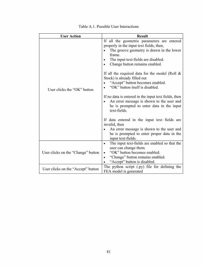
81
Table A.1. Possible User Interactions
User Action Result
User clicks the “OK” button
If all the geometric parameters are entered properly in the input text fields, then, • The groove geometry is drawn in the lower
frame. • The input text-fields are disabled. • Change button remains enabled. If all the required data for the model (Roll & Stock) is already filled out • “Accept” button becomes enabled. • “OK” button itself is disabled. If no data is entered in the input text fields, then• An error message is shown to the user and
he is prompted to enter data in the input text-fields.
If data entered in the input text fields are invalid, then • An error message is shown to the user and
he is prompted to enter proper data in the input text-fields.
User clicks on the “Change” button
• The input text-fields are enabled so that the user can change them.
• “OK” button becomes enabled. • “Change” button remains enabled. • “Accept” button is disabled.
User clicks on the “Accept” button The python script (.py) file for defining the FEA model is generated

82
Figure A.4. Screen layout of the groove geometry Module. A.4.2.2. Roll Properties
The screen layout for this module is shown in Figure A.5. The user inputs the data related to Roll Material properties in this module. These include Roll Type (RIGID / DEFORMABLE) and Roll density. In this work only rigid rolls are considered. “OK”, “Change”, “Accept” button functions in the same way as described in the Roll & Groove Geometry Module.

83
Figure A.5. Screen Layout of the Roll Properties Module.
A.4.2.3. Roll Boundary Conditions
The screen layout for this module is shown in Figure A.6. The user inputs the Rotational Speed of Rolls of successive rolling stands as boundary conditions in this module. “OK”, “Change”, “Accept” button functions in the same way as described in the Roll & Groove Geometry Module.

84
Figure A.6. Screen Layout of the Roll Boundary Conditions Module.
A.4.2.4. Feed Section Geometry
The user enters the input data related to the Feed Section (input stock at the 1st Stand) geometry in this module. The stock geometry module is shown in Figure A.7. The stock can be specified in two ways as shown by the radio buttons in Figure A.7. If the stock is a perfect circle then a radius is only required as shown in Figure A.7. In general a stock is not a perfect circle and can be defined though a file that specifies the (X, Y) coordinates of surface points on the stock section. The file containing the geometric location of surface points is input though the input window as shown in Figure A.8. The software assumes that the origin (0,0) is located at the geometric center of the stock cross section. “OK”, “Change”, “Accept” button functions in the same way as described in the Roll & Groove Geometry Module.

85
Figure A.7. Screen layout for entering stock geometry data
Figure A.8. Screen layout for specifying the file, which contains stock geometry data for
stock geometry Module.

86
A.4.2.5. Stock Properties
The screen layout for this module is shown in Figure A.9. The user inputs the data related to the Material properties of the stock (rod/bar) that include Density, Young’s modulus, Poisson's ratio, Yield point, Specific Heat and Heat Conversion Fraction in this module. The number of points for defining the plastic region can be specified in the last input text-field. After this input text-field is specified the user can click on the “Get data for stress strain curve” button to get actual Flow Stress Data corresponding to Plastic Strain and Temperature. On clicking this button a new window opens up (Figure A.10). User can enter the Plastic Strain data in table shown in this window. On clicking “OK” button in this window the data is stored and the window closes itself. “OK”, “Change”, “Accept” button functions in the same way as described in the Roll & Groove Geometry Module.
Figure A.9. Screen Layout of the Material data Module.

87
Figure A.10. Screen layout for entering plastic strain curve. A.4.2.6. Stock Initial Conditions
The user specifies input data related to initial conditions of the stock in this module. The stock initial conditions module is shown in Figures A.11. Initial velocity in the Rolling direction and Temperature is required as input in this module.
Figure A.11. Screen layout stock initial conditions Module.

88
“OK”, “Change”, “Accept” button functions in the same way as described in the Roll & Groove Geometry Module. A.4.2.7. Stock Meshing Module
The screen layout for this module is shown in Figure A.12. The user inputs the Element Shape, Element library, Element Geometric Order, Kinematic Split Options and Hourglassing Options in this module.
“OK”, “Change”, “Accept” button functions in the same way as described in the
Roll & Groove Geometry module.
Figure A.12. Screen layout stock meshing Module.
A.4.2.8. Contact Information
The screen layout for this module is shown in Figure A.13. The user inputs the Roll/Stock contact behavior including normal contact behavior, tangential contact behavior and coulomb friction co-efficient between Roll and Stock in this module.

89
“OK”, “Change”, “Accept” button functions in the same way as described in the Roll & Groove Geometry module.
Figure A.12. Screen layout Roll/Stock Contact Information Module.
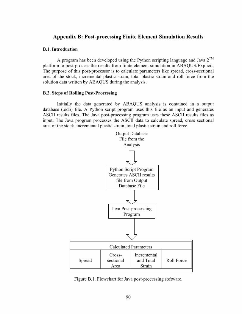
90
Appendix B: Post-processing Finite Element Simulation Results B.1. Introduction
A program has been developed using the Python scripting language and Java 2TM platform to post-process the results from finite element simulation in ABAQUS/Explicit. The purpose of this post-processor is to calculate parameters like spread, cross-sectional area of the stock, incremental plastic strain, total plastic strain and roll force from the solution data written by ABAQUS during the analysis. B.2. Steps of Rolling Post-Processing
Initially the data generated by ABAQUS analysis is contained in a output database (.odb) file. A Python script program uses this file as an input and generates ASCII results files. The Java post-processing program uses these ASCII results files as input. The Java program processes the ASCII data to calculate spread, cross sectional area of the stock, incremental plastic strain, total plastic strain and roll force.
Figure B.1. Flowchart for Java post-processing software.
Output Database File from the
Analysis
Python Script Program Generates ASCII results
file from Output Database File
Java Post-processing Program
Calculated Parameters
Spread Cross-
sectional Area
Incremental and Total
Strain Roll Force
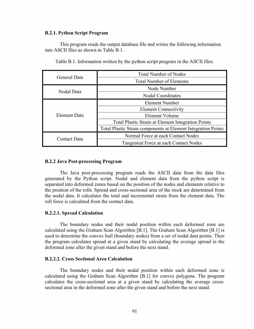
91
B.2.1. Python Script Program This program reads the output database file and writes the following information into ASCII files as shown in Table B.1.
Table B.1. Information written by the python script program in the ASCII files.
Total Number of Nodes General Data Total Number of Elements
Node Number Nodal Data Nodal Coordinates Element Number
Element Connectivity Element Volume
Total Plastic Strain at Element Integration Points Element Data
Total Plastic Strain components at Element Integration Points Normal Force at each Contact Nodes Contact Data
Tangential Force at each Contact Nodes B.2.2 Java Post-processing Program The Java post-processing program reads the ASCII data from the data files generated by the Python script. Nodal and element data from the python script is separated into deformed zones based on the position of the nodes and elements relative to the position of the rolls. Spread and cross-sectional area of the stock are determined from the nodal data. It calculates the total and incremental strain from the element data. The roll force is calculated from the contact data. B.2.2.1. Spread Calculation The boundary nodes and their nodal position within each deformed zone are calculated using the Graham Scan Algorithm [B.1]. The Graham Scan Algorithm [B.1] is used to determine the convex hull (boundary nodes) from a set of nodal data points. Then the program calculates spread at a given stand by calculating the average spread in the deformed zone after the given stand and before the next stand. B.2.2.2. Cross Sectional Area Calculation The boundary nodes and their nodal position within each deformed zone is calculated using the Graham Scan Algorithm [B.1] for convex polygons. The program calculates the cross-sectional area at a given stand by calculating the average cross-sectional area in the deformed zone after the given stand and before the next stand.

92
B.2.2.3. Total Plastic Strain Calculation
The program calculates the total plastic strain at a given stand by calculating the volume averaged total plastic strain in the deformed zone after the given stand and before the next stand as follows (Lee et al. [B.3]):
1
1
e
e
Ni i
T iN
i
i
V
V
εε =
=
=∑
∑ (B.1a)
where iε is the total plastic strain at the ith element, iV is the volume of the ith element and Ne is the number of elements in the deformed zone. B.2.2.4. Incremental Plastic Strain Calculation
To calculate the incremental strain at a given stand the following method is used. First the deformed zone after the given stand and before the next stand is selected. After that individual elements in this deformed zone is identified. Increments in strain components of these elements are calculated by subtracting the total strain component data before deformation at the given stand (this data is available in the time dependent history output) from the final total strain component data. Then the following relation [B.2] calculates incremental plastic strain at ith element
( ) ( ) ( ) ( ) ( ) ( ){ }2 2 2 2 2 22 2 2 23
i i i i i i ixx yy zz xy yz zxε ε ε ε ε ε ε∆ = ∆ + ∆ + ∆ + ∆ + ∆ + ∆ (B.2a)
where iijε∆ is the incremental strain components at the ith element and iε∆ is the
incremental plastic strain at the ith element. The incremental effective plastic strain is calculated by volume averaging the
incremental plastic strain at each element as follows (Lee et al. [B.3]):
1
1
e
e
Ni i
iN
i
i
V
V
εε =
=
∆ =∑
∑ (B.2b)
where ε∆ is the incremental plastic strain at the ith element, iV is the volume of the ith element and Ne is the number of elements in the deformed zone.
B.2.2.5. Roll Force Calculation
The program calculates the role force at a particular stand by adding up all the normal and tangential nodal forces at the nodes where the roll and stock is in contact at that stand in the direction perpendicular to both the direction of rolling and roll axes.
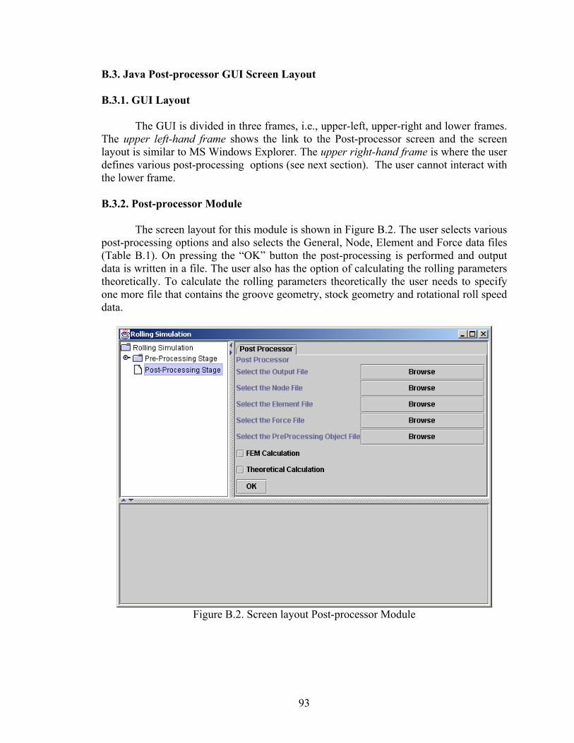
93
B.3. Java Post-processor GUI Screen Layout B.3.1. GUI Layout
The GUI is divided in three frames, i.e., upper-left, upper-right and lower frames. The upper left-hand frame shows the link to the Post-processor screen and the screen layout is similar to MS Windows Explorer. The upper right-hand frame is where the user defines various post-processing options (see next section). The user cannot interact with the lower frame. B.3.2. Post-processor Module
The screen layout for this module is shown in Figure B.2. The user selects various post-processing options and also selects the General, Node, Element and Force data files (Table B.1). On pressing the “OK” button the post-processing is performed and output data is written in a file. The user also has the option of calculating the rolling parameters theoretically. To calculate the rolling parameters theoretically the user needs to specify one more file that contains the groove geometry, stock geometry and rotational roll speed data.
Figure B.2. Screen layout Post-processor Module

94
Appendix C: Initial Finite Element Mesh C.1. Overview
To ensure solution quality throughout a rolling simulation the initial finite element mesh is very important. This section discusses the initial bar/rod geometry, creating a symmetrical mesh, element distortion metrics and element size. C.2. Rod and Bar Geometry
In the finishing stages of bar and rod rolling the input geometry is a prismatic solid cylinder or a polyhedral. The solid in reality is not prismatic, however, is assumed prismatic. The cross-sectional geometry of the stock is either round or oval. In this work the geometric bar/rod model will be approximated as completely round. In each case the cross-section of the stock is symmetrical along the plane going through the center of the stock and parallel to roll axes and symmetrical along the plane perpendicular to this plane as shown in Figure C.1. Cartesian coordinate system is used to define the axes and Z-axis is always taken as the rolling direction axis. Since the roll geometries are also symmetric, and if misalignment is neglected between the rolls and the stock, the problem can be considered to have two perpendicular planes of symmetry in the cross-section. Misalignment between the rolls and the stock can be neglected since it is very small. Therefore, to improve solution quality and to almost ensure a symmetric solution, a symmetric initial mesh will be constructed in this work.
Figure C.1. Planes of symmetry in a typical rod/bar.
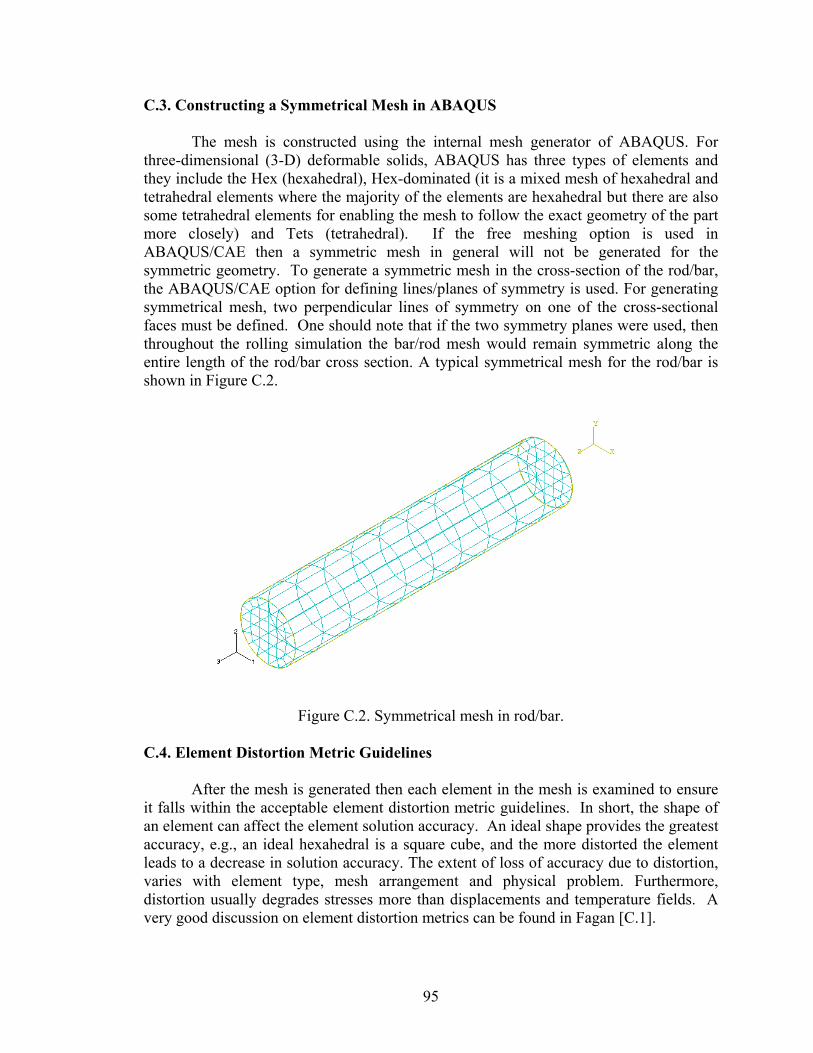
95
C.3. Constructing a Symmetrical Mesh in ABAQUS The mesh is constructed using the internal mesh generator of ABAQUS. For three-dimensional (3-D) deformable solids, ABAQUS has three types of elements and they include the Hex (hexahedral), Hex-dominated (it is a mixed mesh of hexahedral and tetrahedral elements where the majority of the elements are hexahedral but there are also some tetrahedral elements for enabling the mesh to follow the exact geometry of the part more closely) and Tets (tetrahedral). If the free meshing option is used in ABAQUS/CAE then a symmetric mesh in general will not be generated for the symmetric geometry. To generate a symmetric mesh in the cross-section of the rod/bar, the ABAQUS/CAE option for defining lines/planes of symmetry is used. For generating symmetrical mesh, two perpendicular lines of symmetry on one of the cross-sectional faces must be defined. One should note that if the two symmetry planes were used, then throughout the rolling simulation the bar/rod mesh would remain symmetric along the entire length of the rod/bar cross section. A typical symmetrical mesh for the rod/bar is shown in Figure C.2.
Figure C.2. Symmetrical mesh in rod/bar. C.4. Element Distortion Metric Guidelines
After the mesh is generated then each element in the mesh is examined to ensure it falls within the acceptable element distortion metric guidelines. In short, the shape of an element can affect the element solution accuracy. An ideal shape provides the greatest accuracy, e.g., an ideal hexahedral is a square cube, and the more distorted the element leads to a decrease in solution accuracy. The extent of loss of accuracy due to distortion, varies with element type, mesh arrangement and physical problem. Furthermore, distortion usually degrades stresses more than displacements and temperature fields. A very good discussion on element distortion metrics can be found in Fagan [C.1].
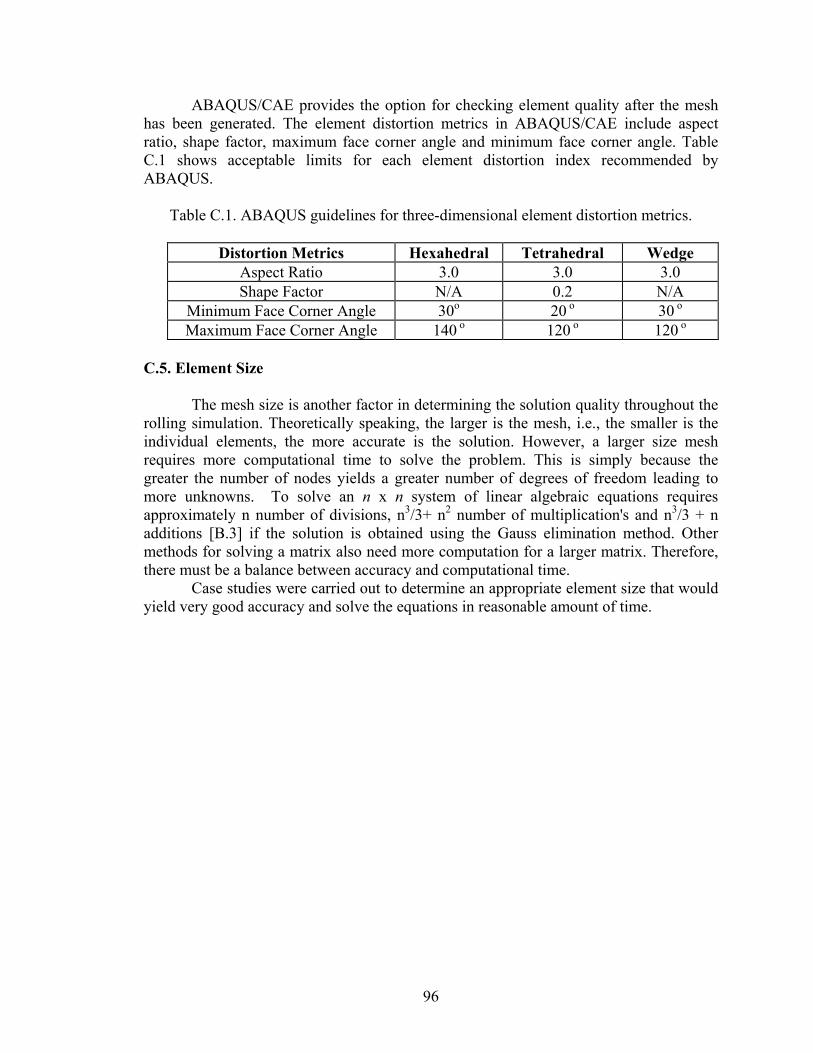
96
ABAQUS/CAE provides the option for checking element quality after the mesh has been generated. The element distortion metrics in ABAQUS/CAE include aspect ratio, shape factor, maximum face corner angle and minimum face corner angle. Table C.1 shows acceptable limits for each element distortion index recommended by ABAQUS.
Table C.1. ABAQUS guidelines for three-dimensional element distortion metrics.
Distortion Metrics Hexahedral Tetrahedral Wedge Aspect Ratio 3.0 3.0 3.0 Shape Factor N/A 0.2 N/A
Minimum Face Corner Angle 30o 20 o 30 o Maximum Face Corner Angle 140 o 120 o 120 o
C.5. Element Size
The mesh size is another factor in determining the solution quality throughout the rolling simulation. Theoretically speaking, the larger is the mesh, i.e., the smaller is the individual elements, the more accurate is the solution. However, a larger size mesh requires more computational time to solve the problem. This is simply because the greater the number of nodes yields a greater number of degrees of freedom leading to more unknowns. To solve an n x n system of linear algebraic equations requires approximately n number of divisions, n3/3+ n2 number of multiplication's and n3/3 + n additions [B.3] if the solution is obtained using the Gauss elimination method. Other methods for solving a matrix also need more computation for a larger matrix. Therefore, there must be a balance between accuracy and computational time.
Case studies were carried out to determine an appropriate element size that would yield very good accuracy and solve the equations in reasonable amount of time.

97
Appendix D: Full Scale Mill Testing
A series of tests were conducted on one of Morgan’s [D.1] RSM units installed in a rod production line in order to gather detailed dimensional data on the rolling stock for comparison with the finite element model and theoretical model in the next section. A standard size rod product of AISI 1045 carbon steel was rolled in a series of tests in which the entry temperature to the RSM, the rolling rate and the entry dimensions were all held constant. The tests consisted of rolling a billet through four stands of the RSM to obtain rod samples.
Samples of the rolled product were obtained after the rod had passed through water cooling boxes, formed into continuous loops by the laying head and cooled on the air-cooling conveyor. Short samples were cut from the coils produced from each test. For dimensional measurement, the samples were placed in a custom-made system for detailed off-line dimensional measurements of rod and bar products using a laser gauge and specialized analysis software. Diameter measurements were obtained for sixty diametrical locations, giving a detailed representation of the stock geometry profile. The measurements are carried out for RSM feed section, exit of stand #2, exit of stand #3 and exit of stand #4. The obtained data is shown in Table D.1
Table D.1. Dimension measurements of stock samples from RSM Full-scale mill Testing
Measurements at RSM feed section Angle Diameter Angle Diameter Angle Diameter
0 16.4699 63 16.3525 126 16.4428 3 16.4741 66 16.3782 129 16.4494 6 16.4707 69 16.3880 132 16.4627 9 16.4551 72 16.3979 135 16.4844
12 16.4387 75 16.4043 138 16.5055 15 16.4346 78 16.4117 141 16.5026 18 16.4246 81 16.4327 144 16.4848 21 16.4130 84 16.4396 147 16.4796 24 16.4012 87 16.4438 150 16.4785 27 16.3955 90 16.4689 153 16.4793 30 16.3764 93 16.4737 156 16.4780 33 16.3692 96 16.4789 159 16.4769 36 16.3685 99 16.4499 162 16.4737 39 16.3598 102 16.3899 165 16.4702 42 16.3527 105 16.3830 168 16.4605 45 16.3367 108 16.4032 171 16.4585 48 16.3026 111 16.4175 174 16.4611 51 16.2773 114 16.4277 177 16.4595 54 16.2495 117 16.4372 180 16.4557 57 16.2733 120 16.4413 60 16.3213 123 16.4411

98
Measurements at Exit of Stand #2
Angle Diameter Angle Diameter Angle Diameter 0 13.4975 63 13.7204 126 13.6503 3 13.4806 66 13.7925 129 13.6421 6 13.4689 69 13.8360 132 13.6359 9 13.4572 72 13.8711 135 13.6283
12 13.4424 75 13.9057 138 13.6190 15 13.4295 78 13.9306 141 13.6115 18 13.4189 81 13.9643 144 13.6057 21 13.4102 84 13.9887 147 13.6017 24 13.4048 87 13.9971 150 13.5919 27 13.3941 90 14.0065 153 13.5820 30 13.3912 93 14.0092 156 13.5738 33 13.3825 96 13.9977 159 13.5584 36 13.3769 99 13.9677 162 13.5440 39 13.3702 102 13.9089 165 13.5490 42 13.3641 105 13.8216 168 13.5433 45 13.3601 108 13.7561 171 13.5225 48 13.3564 111 13.6966 174 13.5108 51 13.3726 114 13.6700 177 13.5092 54 13.4261 117 13.6646 180 13.4951 57 13.5079 120 13.6569 60 13.6159 123 13.6550
Measurements at Exit of Stand #3 Angle Diameter Angle Diameter Angle Diameter
0 12.5497 63 12.8083 126 13.7836 3 12.5420 66 12.8695 129 13.7120 6 12.5395 69 12.9954 132 13.6209 9 12.5406 72 13.1725 135 13.4982
12 12.5368 75 13.3578 138 13.3434 15 12.5210 78 13.5101 141 13.1699 18 12.5102 81 13.6266 144 12.9973 21 12.5081 84 13.7107 147 12.8736 24 12.5175 87 13.7640 150 12.8170 27 12.5323 90 13.8109 153 12.7816 30 12.5443 93 13.8648 156 12.7468 33 12.5571 96 13.9132 159 12.7194 36 12.5731 99 13.9484 162 12.6905 39 12.5920 102 13.9711 165 12.6618 42 12.6122 105 13.9864 168 12.6313 45 12.6387 108 13.9882 171 12.6066 48 12.6623 111 13.9809 174 12.5860 51 12.6848 114 13.9649 177 12.5679 54 12.7122 117 13.9372 180 12.5526 57 12.7427 120 13.8956 60 12.7754 123 13.8426

99
Measurements at Exit of Stand #4
Angle Diameter Angle Diameter Angle Diameter 0 12.7711 63 12.7614 126 12.8015 3 12.7692 66 12.7599 129 12.8048 6 12.7677 69 12.7570 132 12.8085 9 12.7685 72 12.7524 135 12.8103
12 12.7680 75 12.7528 138 12.8143 15 12.7695 78 12.7545 141 12.8151 18 12.7658 81 12.7578 144 12.8162 21 12.7628 84 12.7557 147 12.8137 24 12.7604 87 12.7547 150 12.8064 27 12.7562 90 12.7560 153 12.7938 30 12.7554 93 12.7711 156 12.7855 33 12.7564 96 12.7900 159 12.7819 36 12.7567 99 12.7958 162 12.7789 39 12.7597 102 12.7974 165 12.7776 42 12.7606 105 12.7963 168 12.7754 45 12.7592 108 12.7983 171 12.7723 48 12.7604 111 12.7966 174 12.7688 51 12.7594 114 12.7980 177 12.7709 54 12.7612 117 12.7943 180 12.7720 57 12.7616 120 12.7954 60 12.7634 123 12.7984

100
Appendix E: Important Aspects of the Finite Element Model The table below provides some details regarding the finite elements models used in Tables 5.3 and 5.12.
Mesh Domain
Two types of solution techniques are used in solving this problem. The first kind of formulation involves traditional pure Lagrangian formulation where the mesh is constrained to the material. The second kind of formulation combines features of both pure Eulerian formulation (in which the mesh is fixed spatially and the material flows through the mesh) and pure Lagrangian formulation. In this case Adaptive meshing is used and is referred to as the Arbitrary Lagrangian-Eulerian (ALE) formulation. This approach often eliminates excessive mesh distortions that are associated with a Lagrangian analysis involving large deformation. Using this approach, the inlet of the stock was defined with Eulerian constraints in order to permit material flow; the mesh on this face was spatially constrained in all directions. The material on the radial surface of the stock was constrained to the mesh in the direction normal to the free surface but was permitted to flow relative to the mesh in the tangential direction.
Time Dependence In this work the problem is considered as transient.
Time Integration
Explicit, Dynamics, Adiabatic method is used in this work. In this method a large number of time steps is used with very small increments. This method is suitable for high-speed dynamic events like our case where stress wave propagation requires the increment to of very small size to capture wave propagation. Implicit methods can be very costly in this type of problems especially in the case of three-dimensional formulation.
Dimensionality
A full three-dimensional finite element model is considered in this work.
Formulation
Mass Scaling
Mass scaling is often used to increase the stable time increment of an non-linear analysis by reducing the effects of mass matrix in the solution but it also contributes to the inaccuracies in the solution especially in the parameters that depends on inertia. The author has carried out a study on the effect of mass scaling on the finite element solution and found the result to be unsatisfactory. In this work we do not use mass scaling.

101
Adaptive Meshing
Adaptive meshing is often used to control excessive mesh distortion, which often occurs in non-linear problems. In adaptive mass scaling after a certain number of time steps the entire geometry of the body is remeshed. We this method for the ALE formulation only.
Hourglass
One disadvantage of using reduced integration procedure is that it can admit deformation modes, which cause no straining at the integration points. These zero energy modes make the element rank deficient and cause a phenomenon called hourglassing where, the zero energy modes starts propagating through the mesh leading to inaccurate solutions. This problem is particularly severe in hexahedral elements. To counter this a small artificial stiffness is attached with the zero energy and is associated with the zero energy deformation modes. This procedure is called hourglass control. In this work, we select the hourglass control as "Stiffness" was used.

102
Element Type
Three-dimensional, Deformable, Reduced Integration, Linear Hexahedral (Brick) element (C3D8R) is used in this work. There are two advantages of using Reduced integration elements. First, stresses and strains are calculated in the so-called Barlow Points [] providing optimal accuracy. Second, the computational time is less due to reduced number of integration points.
Material Stock material is assumed as homogeneous and isotropic material with no porosities.
Rate Dependence The stock material is assumed to be strain rate dependent.
Plasticity Law Three main plasticity laws are used in this work. They are Shida [E.2], Modified Shida [E.3] and Lee [E.4].
Hardening Rate Isotropic
% Plastic Deformation Energy Converted to Heat
In an adiabatic analysis a portion of the energy of plastic deformation converts into heat. In this work we consider this ratio to be 0.90.
Stock
Initial Conditions
Two initial conditions are mainly used in this work. They are 1) Initial velocity of the stock i.e. the velocity of the stock when it enters the first stand and 2) Initial temperature of the stock i.e. the temperature of the stock when it enters the first stand.
Material Tungsten carbide Finite Element Characterization
The rolls are considered as analytic rigid surface in this work. Roll
Boundary Conditions
Angular velocity of rolls are used as the boundary conditions for this work
Contact Condition
Contact between roll and stock is defined as a contact pair that consist of penalty contact enforcement method, balanced contact surface weighting and finite sliding formulation is used.
Friction Model Coulomb friction model is used for this work with µ=0.3
Stock / Roll Interface
Heat Transfer Effects Heat transfer effects are not considered
Stand Material Stand is considered as a rigid pin support

103
Appendix F: Additional Finite Element Analyses F.1. Results of Finite Element Solution for the RSM Case (Section 5.2)
In this section detailed results of the finite element model solved by different formulation types, constitutive models for plastic behavior and different mesh sizes are presented. Tables F.1 through F.7 summarizes the finite element, theoretical and full-scale mill testing results for spread, cross-sectional area, percentage reduction in area, incremental plastic strain, total plastic strain and roll force at all four finishing stands. Overall it can be observed from finite element solutions obtained using Lagrangian formulation yields marginally better results than finite element solutions obtained using Arbitrary Lagrangian-Eulerian (ALE) formulation. It is also observed that effect of using different constitutive models on geometric and deformation parameters is practically non-existent. Therefore it can be concluded that stock deformation in finishing rolling stage doesn’t depend on constitutive laws. But it is observed that the It is also observed that effect of using different constitutive models on roll force is significant and cannot be neglected. It was observed that the roll force obtained by the finite element solution using Modified Shida [F.1] constitutive law is most consistent with a proprietary Morgan [F.5] technique for calculating roll force. The proprietary model employs a combination of empirical techniques and experimental validation.
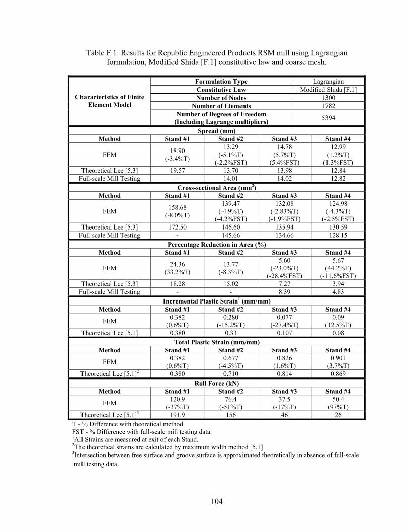
104
Table F.1. Results for Republic Engineered Products RSM mill using Lagrangian formulation, Modified Shida [F.1] constitutive law and coarse mesh.
Formulation Type Lagrangian Constitutive Law Modified Shida [F.1] Number of Nodes 1300
Number of Elements 1782 Characteristics of Finite
Element Model Number of Degrees of Freedom
(Including Lagrange multipliers) 5394
Spread (mm) Method Stand #1 Stand #2 Stand #3 Stand #4
FEM 18.90 (-3.4%T)
13.29 (-5.1%T)
(-2.2%FST)
14.78 (5.7%T)
(5.4%FST)
12.99 (1.2%T)
(1.3%FST) Theoretical Lee [5.3] 19.57 13.70 13.98 12.84
Full-scale Mill Testing - 14.01 14.02 12.82 Cross-sectional Area (mm2)
Method Stand #1 Stand #2 Stand #3 Stand #4
FEM 158.68 (-8.0%T)
139.47 (-4.9%T)
(-4.2%FST)
132.08 (-2.83%T)
(-1.9%FST)
124.98 (-4.3%T)
(-2.5%FST) Theoretical Lee [5.3] 172.50 146.60 135.94 130.59
Full-scale Mill Testing - 145.66 134.66 128.15 Percentage Reduction in Area (%)
Method Stand #1 Stand #2 Stand #3 Stand #4
FEM 24.36 (33.2%T)
13.77 (-8.3%T)
5.60 (-23.0%T)
(-28.4%FST)
5.67 (44.2%T)
(-11.6%FST) Theoretical Lee [5.3] 18.28 15.02 7.27 3.94
Full-scale Mill Testing - - 8.39 4.83 Incremental Plastic Strain1 (mm/mm)
Method Stand #1 Stand #2 Stand #3 Stand #4
FEM 0.382 (0.6%T)
0.280 (-15.2%T)
0.077 (-27.4%T)
0.09 (12.5%T)
Theoretical Lee [5.1] 0.380 0.33 0.107 0.08 Total Plastic Strain (mm/mm)
Method Stand #1 Stand #2 Stand #3 Stand #4
FEM 0.382 (0.6%T)
0.677 (-4.5%T)
0.826 (1.6%T)
0.901 (3.7%T)
Theoretical Lee [5.1]2 0.380 0.710 0.814 0.869 Roll Force (kN)
Method Stand #1 Stand #2 Stand #3 Stand #4
FEM 120.9 (-37%T)
76.4 (-51%T)
37.5 (-17%T)
50.4 (97%T)
Theoretical Lee [5.1]3 191.9 156 46 26 T - % Difference with theoretical method. FST - % Difference with full-scale mill testing data. 1All Strains are measured at exit of each Stand. 2The theoretical strains are calculated by maximum width method [5.1] 3Intersection between free surface and groove surface is approximated theoretically in absence of full-scale mill testing data.

105
Table F.2. Results for Republic Engineered Products RSM mill using Lagrangian formulation, Modified Shida [F.1] constitutive law and medium mesh.
Formulation Type Lagrangian Constitutive Law Modified Shida [F.1] Number of Nodes 7800
Number of Elements 9563 Characteristics of Finite
Element Model Number of Degrees of Freedom
(Including Lagrange multipliers) 27737
Spread (mm) Method Stand #1 Stand #2 Stand #3 Stand #4
FEM 19.13 (-2.3%T)
13.76 (0.5%T)
(-1.5%FST)
14.71 (4.9%T)
(5.3%FST)
12.94 (0.8%T)
(0.9%FST) Theoretical Lee [5.3] 19.57 13.70 13.98 12.84
Full-scale Mill Testing - 14.01 14.02 12.82 Cross-sectional Area (mm2)
Method Stand #1 Stand #2 Stand #3 Stand #4
FEM 166.84 (-3.3%T)
145.74 (-0.6%T)
(1.8%FST)
134.88 (-0.8%T)
(2.0%FST)
128.53 (-1.6%T)
(0.5%FST) Theoretical Lee [5.3] 172.50 146.60 135.94 130.59
Full-scale Mill Testing - 145.66 134.66 128.15 Percentage Reduction in Area (%)
Method Stand #1 Stand #2 Stand #3 Stand #4
FEM 22.6 (23.5%T)
14.47 (-3.6%T)
8.05 (10.7%T)
(-4.05%FST)
4.94 (25.6%T)
(-2.2%FST) Theoretical Lee [5.3] 18.28 15.02 7.27 3.94
Full-scale Mill Testing - - 8.39 4.83 Incremental Plastic Strain1 (mm/mm)
Method Stand #1 Stand #2 Stand #3 Stand #4
FEM 0.388 (2.4%T)
0.320 (-3.0%T)
0.112 (5.5%T)
0.0875 (9.3%T)
Theoretical Lee [5.1] 0.380 0.33 0.107 0.08 Total Plastic Strain (mm/mm)
Method Stand #1 Stand #2 Stand #3 Stand #4
FEM 0.388 (2.4%T)
0.740 (4.25%T)
0.903 (11.0%T)
0.974 (12.1%T)
Theoretical Lee [5.1]2 0.380 0.710 0.814 0.869 Roll Force (kN)
Method Stand #1 Stand #2 Stand #3 Stand #4
FEM 112.3 (-41.5%T)
80.3 (-48.5%T)
50.4 (11.4%T)
36.6 (44%T)
Theoretical Lee [5.1]3 191.9 156 46 26 T - % Difference with theoretical method. FST - % Difference with full-scale mill testing data. 1All Strains are measured at exit of each Stand. 2The theoretical strains are calculated by maximum width method [5.1] 3Intersection between free surface and groove surface is approximated theoretically in absence of full-scale mill testing data.

106
Table F.3. Results for Republic Engineered Products RSM mill using Lagrangian formulation, Shida [F.2] constitutive law and coarse mesh.
Formulation Type Lagrangian Constitutive Law Shida [F.2] Number of Nodes 1300
Number of Elements Freedom in the problem 1782 Characteristics of Finite
Element Model Number of Degrees of Freedom
(Including Lagrange multipliers) 5394
Spread (mm) Method Stand #1 Stand #2 Stand #3 Stand #4
FEM 18.88 (-3.4%T)
13.29 (-5.1%T)
(-2.2%FST)
14.75 (5.7%T)
(5.4%FST)
12.99 (1.2%T)
(1.3%FST) Theoretical Lee [5.3] 19.57 13.70 13.98 12.84
Full-scale Mill Testing - 14.01 14.02 12.82 Cross-sectional Area (mm2)
Method Stand #1 Stand #2 Stand #3 Stand #4
FEM 158.6 (-8.1%T)
139.47 (-4.9%T)
(-4.2%FST)
131.9 (-2.9%T)
(-2.0%FST)
124.91 (-4.3%T)
(-2.5%FST) Theoretical Lee [5.3] 172.50 146.60 135.94 130.59
Full-scale Mill Testing - 145.66 134.66 128.15 Percentage Reduction in Area (%)
Method Stand #1 Stand #2 Stand #3 Stand #4
FEM 24.41 (33.5%T)
13.79 (-8.1%T)
5.66 (-22.2%T)
(-28.4%FST)
5.59 (42%T)
(-11.6%FST) Theoretical Lee [5.3] 18.28 15.02 7.27 3.94
Full-scale Mill Testing - - 8.39 4.83 Incremental Plastic Strain1 (mm/mm)
Method Stand #1 Stand #2 Stand #3 Stand #4
FEM 0.381 (0.5%T)
0.277 (-18.2%T)
0.126 (16.7%T)
0.118 (47%T)
Theoretical Lee [5.1] 0.380 0.33 0.107 0.08 Total Plastic Strain (mm/mm)
Method Stand #1 Stand #2 Stand #3 Stand #4
FEM 0.381 (0.5%T)
0.677 (-4.5%T)
0.826 (1.6%T)
0.898 (3.7%T)
Theoretical Lee [5.1]2 0.380 0.710 0.814 0.869 Roll Force (kN)
Method Stand #1 Stand #2 Stand #3 Stand #4
FEM 113 (-40.9%T)
70.9 (-54.6%T)
37.2 (-18.8%T)
40.4 (58.8%T)
Theoretical Lee [5.1]3 191.9 156 46 26 T - % Difference with theoretical method. FST - % Difference with full-scale mill testing data. 1All Strains are measured at exit of each Stand. 2The theoretical strains are calculated by maximum width method [5.1] 3Intersection between free surface and groove surface is approximated theoretically in absence of full-scale mill testing data.

107
Table F.4. Results for Republic Engineered Products RSM mill using Lagrangian formulation, Shida [F.2] constitutive law and medium mesh.
Formulation Type Lagrangian Constitutive Law Shida [F.2] Number of Nodes 7800
Number of Elements 9563 Characteristics of Finite
Element Model Number of Degrees of Freedom
(Including Lagrange multipliers) 27737
Spread (mm) Method Stand #1 Stand #2 Stand #3 Stand #4
FEM 19.09 (-2.4%T)
13.77 (0.5%T)
(-1.5%FST)
14.69 (4.8%T)
(5.3%FST)
12.96 (0.9%T)
(1.1%FST) Theoretical Lee [5.3] 19.57 13.70 13.98 12.84
Full-scale Mill Testing - 14.01 14.02 12.82 Cross-sectional Area (mm2)
Method Stand #1 Stand #2 Stand #3 Stand #4
FEM 166.82 (-3.3%T)
145.73 (-0.6%T)
(1.8%FST)
134.77 (-0.9%T)
(0.9%FST)
128.50 (-1.6%T)
(0.3%FST) Theoretical Lee [5.3] 172.50 146.60 135.94 130.59
Full-scale Mill Testing - 145.66 134.66 128.15 Percentage Reduction in Area (%)
Method Stand #1 Stand #2 Stand #3 Stand #4
FEM 22.6 (23.5%T)
14.46 (-3.6%T)
8.12 (11.8%T) (-4%FST)
4.88 (26.3%T) (-1%FST)
Theoretical Lee [5.3] 18.28 15.02 7.27 3.94 Full-scale Mill Testing - - 8.39 4.83
Incremental Plastic Strain1 (mm/mm) Method Stand #1 Stand #2 Stand #3 Stand #4
FEM 0.388 (2.4%T)
0.320 (-3.0%T)
0.112 (5.5%T)
0.0871 (9%T)
Theoretical Lee [5.1] 0.380 0.33 0.107 0.08 Total Plastic Strain (mm/mm)
Method Stand #1 Stand #2 Stand #3 Stand #4
FEM 0.388 (2.4%T)
0.738 (4%T)
0.898 (10.4%T)
0.971 (11.7%T)
Theoretical Lee [5.1]2 0.380 0.710 0.814 0.869 Roll Force (kN)
Method Stand #1 Stand #2 Stand #3 Stand #4
FEM 108.4 (-43%T)
74.8 (-52%T)
50.9 (11.6%T)
32.1 (26.3%T)
Theoretical Lee [5.1]3 191.9 156 46 26 T - % Difference with theoretical method. FST - % Difference with full-scale mill testing data. 1All Strains are measured at exit of each Stand. 2The theoretical strains are calculated by maximum width method [5.1] 3Intersection between free surface and groove surface is approximated theoretically in absence of full-scale mill testing data.

108
Table F.5. Results for Republic Engineered Products RSM mill using Lagrangian formulation, Shida [F.2] constitutive law and fine mesh.
Formulation Type Lagrangian Constitutive Law Shida [F.2] Number of Nodes 42820
Number of Elements Freedom in the problem 49994 Characteristics of Finite
Element Model Number of Degrees of Freedom
(Including Lagrange multipliers) 147030
Spread (mm) Method Stand #1 Stand #2 Stand #3 Stand #4
FEM 19.10 (-2.4%T)
13.57 (-0.9%T)
(-1.5%FST)
14.43 (2.98%T)
(2.8%FST)
12.83 (-0.1%T)
(0.1%FST) Theoretical Lee [5.3] 19.57 13.70 13.98 12.84
Full-scale Mill Testing - 14.01 14.02 12.82 Cross-sectional Area (mm2)
Method Stand #1 Stand #2 Stand #3 Stand #4
FEM 167.65 (-2.8%T)
145.67 (0.01%T)
(-0.6%FST)
134.83 (-0.8%T)
(0.1%FST)
128.83 (-1.3%T)
(0.5%FST) Theoretical Lee [5.3] 172.50 146.60 135.94 130.59
Full-scale Mill Testing - 145.66 134.66 128.15 Percentage Reduction in Area (%)
Method Stand #1 Stand #2 Stand #3 Stand #4
FEM 22.95 (25.6%T)
15.09 (0.5%T)
8.03 (10.4%T)
(-4.3%FST)
4.66 (18.4%T)
(-3.5%FST) Theoretical Lee [5.3] 18.28 15.02 7.27 3.94
Full-scale Mill Testing - - 8.39 4.83 Incremental Plastic Strain1 (mm/mm)
Method Stand #1 Stand #2 Stand #3 Stand #4
FEM 0.399 (5.2%T)
0.379 (+15.5%T)
0.107 (0.5%T)
0.08 (0.2%T)
Theoretical Lee [5.1] 0.380 0.33 0.107 0.08 Total Plastic Strain (mm/mm)
Method Stand #1 Stand #2 Stand #3 Stand #4
FEM 0.399 (5.2%T)
0.763 (7.51%T)
0.902 (10.9%T)
0.981 (13%T)
Theoretical Lee [5.1]2 0.380 0.710 0.814 0.869 Roll Force (kN)
Method Stand #1 Stand #2 Stand #3 Stand #4
FEM 108.9 (-43.2%T)
79.7 (-48.9%T)
47.2 (3.4%T)
29.7 (16.8%T)
Theoretical Lee [5.1]3 191.9 156 46 26 T - % Difference with theoretical method. FST - % Difference with full-scale mill testing data. 1All Strains are measured at exit of each Stand. 2The theoretical strains are calculated by maximum width method [5.1] 3Intersection between free surface and groove surface is approximated theoretically in absence of full-scale mill testing data.
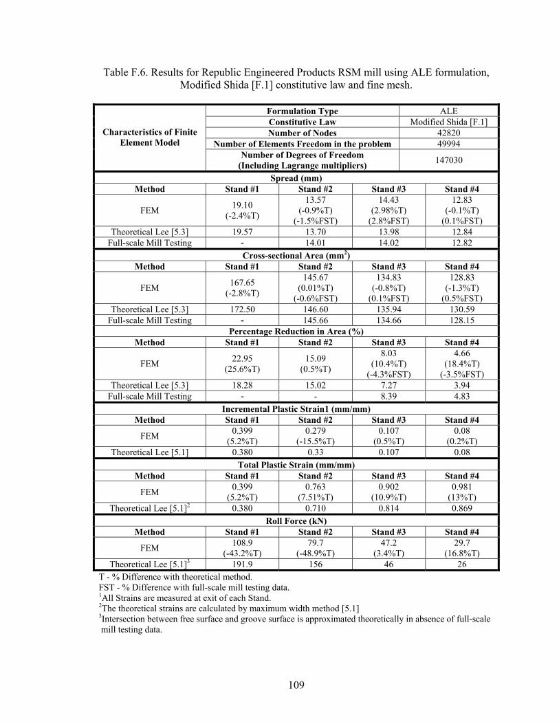
109
Table F.6. Results for Republic Engineered Products RSM mill using ALE formulation, Modified Shida [F.1] constitutive law and fine mesh.
Formulation Type ALE Constitutive Law Modified Shida [F.1] Number of Nodes 42820
Number of Elements Freedom in the problem 49994 Characteristics of Finite
Element Model Number of Degrees of Freedom
(Including Lagrange multipliers) 147030
Spread (mm) Method Stand #1 Stand #2 Stand #3 Stand #4
FEM 19.10 (-2.4%T)
13.57 (-0.9%T)
(-1.5%FST)
14.43 (2.98%T)
(2.8%FST)
12.83 (-0.1%T)
(0.1%FST) Theoretical Lee [5.3] 19.57 13.70 13.98 12.84
Full-scale Mill Testing - 14.01 14.02 12.82 Cross-sectional Area (mm2)
Method Stand #1 Stand #2 Stand #3 Stand #4
FEM 167.65 (-2.8%T)
145.67 (0.01%T)
(-0.6%FST)
134.83 (-0.8%T)
(0.1%FST)
128.83 (-1.3%T)
(0.5%FST) Theoretical Lee [5.3] 172.50 146.60 135.94 130.59
Full-scale Mill Testing - 145.66 134.66 128.15 Percentage Reduction in Area (%)
Method Stand #1 Stand #2 Stand #3 Stand #4
FEM 22.95 (25.6%T)
15.09 (0.5%T)
8.03 (10.4%T)
(-4.3%FST)
4.66 (18.4%T)
(-3.5%FST) Theoretical Lee [5.3] 18.28 15.02 7.27 3.94
Full-scale Mill Testing - - 8.39 4.83 Incremental Plastic Strain1 (mm/mm)
Method Stand #1 Stand #2 Stand #3 Stand #4
FEM 0.399 (5.2%T)
0.279 (-15.5%T)
0.107 (0.5%T)
0.08 (0.2%T)
Theoretical Lee [5.1] 0.380 0.33 0.107 0.08 Total Plastic Strain (mm/mm)
Method Stand #1 Stand #2 Stand #3 Stand #4
FEM 0.399 (5.2%T)
0.763 (7.51%T)
0.902 (10.9%T)
0.981 (13%T)
Theoretical Lee [5.1]2 0.380 0.710 0.814 0.869 Roll Force (kN)
Method Stand #1 Stand #2 Stand #3 Stand #4
FEM 108.9 (-43.2%T)
79.7 (-48.9%T)
47.2 (3.4%T)
29.7 (16.8%T)
Theoretical Lee [5.1]3 191.9 156 46 26 T - % Difference with theoretical method. FST - % Difference with full-scale mill testing data. 1All Strains are measured at exit of each Stand. 2The theoretical strains are calculated by maximum width method [5.1] 3Intersection between free surface and groove surface is approximated theoretically in absence of full-scale mill testing data.
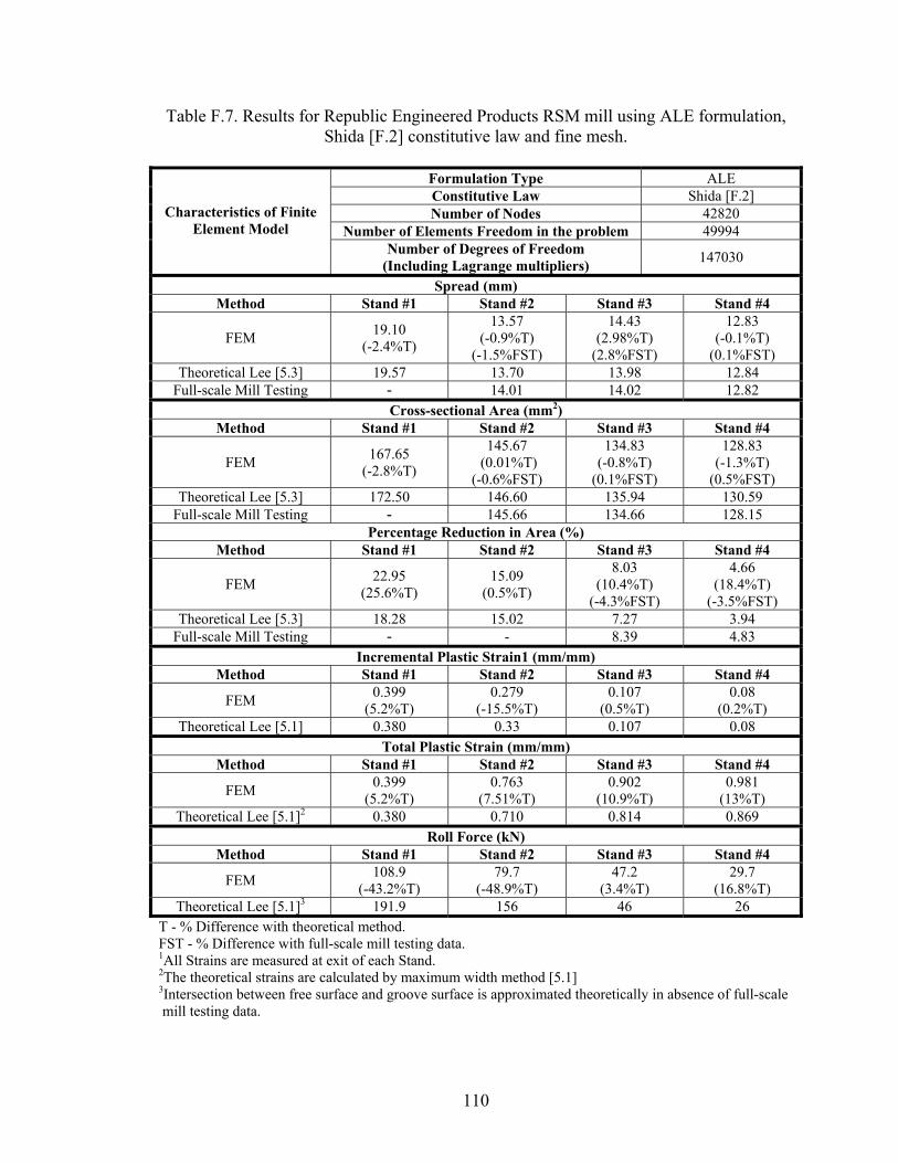
110
Table F.7. Results for Republic Engineered Products RSM mill using ALE formulation, Shida [F.2] constitutive law and fine mesh.
Formulation Type ALE Constitutive Law Shida [F.2] Number of Nodes 42820
Number of Elements Freedom in the problem 49994 Characteristics of Finite
Element Model Number of Degrees of Freedom
(Including Lagrange multipliers) 147030
Spread (mm) Method Stand #1 Stand #2 Stand #3 Stand #4
FEM 19.10 (-2.4%T)
13.57 (-0.9%T)
(-1.5%FST)
14.43 (2.98%T)
(2.8%FST)
12.83 (-0.1%T)
(0.1%FST) Theoretical Lee [5.3] 19.57 13.70 13.98 12.84
Full-scale Mill Testing - 14.01 14.02 12.82 Cross-sectional Area (mm2)
Method Stand #1 Stand #2 Stand #3 Stand #4
FEM 167.65 (-2.8%T)
145.67 (0.01%T)
(-0.6%FST)
134.83 (-0.8%T)
(0.1%FST)
128.83 (-1.3%T)
(0.5%FST) Theoretical Lee [5.3] 172.50 146.60 135.94 130.59
Full-scale Mill Testing - 145.66 134.66 128.15 Percentage Reduction in Area (%)
Method Stand #1 Stand #2 Stand #3 Stand #4
FEM 22.95 (25.6%T)
15.09 (0.5%T)
8.03 (10.4%T)
(-4.3%FST)
4.66 (18.4%T)
(-3.5%FST) Theoretical Lee [5.3] 18.28 15.02 7.27 3.94
Full-scale Mill Testing - - 8.39 4.83 Incremental Plastic Strain1 (mm/mm)
Method Stand #1 Stand #2 Stand #3 Stand #4
FEM 0.399 (5.2%T)
0.279 (-15.5%T)
0.107 (0.5%T)
0.08 (0.2%T)
Theoretical Lee [5.1] 0.380 0.33 0.107 0.08 Total Plastic Strain (mm/mm)
Method Stand #1 Stand #2 Stand #3 Stand #4
FEM 0.399 (5.2%T)
0.763 (7.51%T)
0.902 (10.9%T)
0.981 (13%T)
Theoretical Lee [5.1]2 0.380 0.710 0.814 0.869 Roll Force (kN)
Method Stand #1 Stand #2 Stand #3 Stand #4
FEM 108.9 (-43.2%T)
79.7 (-48.9%T)
47.2 (3.4%T)
29.7 (16.8%T)
Theoretical Lee [5.1]3 191.9 156 46 26 T - % Difference with theoretical method. FST - % Difference with full-scale mill testing data. 1All Strains are measured at exit of each Stand. 2The theoretical strains are calculated by maximum width method [5.1] 3Intersection between free surface and groove surface is approximated theoretically in absence of full-scale mill testing data.

111
F.2. Results of Finite Element solution for the POSCO case (Section 5.3) In this section detailed results of the finite element model solved by different
formulation types, different constitutive model for plastic behavior and different mesh sizes are presented tables F.8 to F.10. Tables F.8 to F.10 summarizes the finite element and theoretical for spread, cross-sectional area, percentage reduction in area, incremental plastic strain, total plastic strain and roll force at all four finishing stands. Overall it can be observed from finite element solutions obtained using Lagrangian formulation yields marginally better results than finite element solutions obtained using Arbitrary Lagrangian-Eulerian (ALE) formulation. It is also observed that effect of using different constitutive models on geometric and deformation parameters is practically non-existent. Therefore it can be concluded that stock deformation in finishing rolling stage doesn’t depend on constitutive laws. But it is observed that the It is also observed that effect of using different constitutive models on roll force is significant and cannot be neglected. It was observed that the roll force obtained by the finite element solution using Modified Shida [F.1] constitutive law is most consistent with a proprietary Morgan [F.5] technique for calculating roll force. The proprietary model employs a combination of empirical techniques and experimental validation.

112
Table F.8. Results for POSCO No.3 mill using Lagrangian formulation, Suzuki [F.3] constitutive law and medium mesh.
Formulation Type Lagrangian Constitutive Law Suzuki [F.3] Number of Nodes 3456
Number of Elements Freedom in the problem 4753 Characteristics of Finite
Element Model Number of Degrees of Freedom
(Including Lagrange multipliers) 14307
Spread (mm) Method Stand #1 Stand #2 Stand #3 Stand #4
FEM 183.40 (-2.3%T)
196.47 (7.7%T)
114.69 (-2.8%T)
142.62 (-6.1%T)
Theoretical Lee [5.3] 187.65 182.46 118.01 151.80 Cross-sectional Area (mm2)
Method Stand #1 Stand #2 Stand #3 Stand #4
FEM 20451.25 (-1.8%T)
14547.11 (2.2%T)
10825.74 (-2.4%T)
8119.21 (-2.4%T)
Theoretical Lee [5.3] 20828.64 14237.84 11092.66 8320.964 Percentage Reduction in Area (%)
Method Stand #1 Stand #2 Stand #3 Stand #4
FEM 27.42 (32.9%T)
40.60 (28.3%T)
34.37 (55.6 %T)
33.33 (33.3%T)
Theoretical Lee [5.3] 20.63 31.64 22.09 24.99 Incremental Plastic Strain1 (mm/mm)
Method Stand #1 Stand #2 Stand #3 Stand #4
FEM 0.41 (7%T)
0.74 (-9%T)
0.51 (1.7%T)
0.47 (-13.5%T)
Theoretical Lee [5.1] 0.381 0.808 0.499 0.540 Total Plastic Strain (mm/mm)
Method Stand #1 Stand #2 Stand #3 Stand #4
FEM 0.41 (7%T)
1.25 (5.4%T)
1.80 (6.6%T)
2.12 (-4.5%T)
Theoretical Lee [5.1]2 0.381 1.186 1.685 2.22 Roll Force (kN)
Method Stand #1 Stand #2 Stand #3 Stand #4
FEM 2403.12 (-29.2%T)
2670.69 (-34.4%T)
1998.42 (-37.4%T)
1684.73 (-47.1%T)
Theoretical Lee [5.1]3 3394 4069 3196 3182 T - % Difference with theoretical method. 1All Strains are measured at exit of each Stand. 2The theoretical strains are calculated by maximum width method [5.1] 3Intersection between free surface and groove surface is approximated theoretically in absence of full-scale mill testing data.

113
Table F.9. Results for POSCO No.3 mill using Lagrangian formulation, Shida [F.2] constitutive law and medium mesh.
Formulation Type ALE Constitutive Law Suzuki [F.2] Number of Nodes 3456
Number of Elements Freedom in the problem 4753 Characteristics of Finite
Element Model Number of Degrees of Freedom
(Including Lagrange multipliers) 14307
Spread (mm) Method Stand #1 Stand #2 Stand #3 Stand #4
FEM 183.40 (-2.3%T)
196.47 (7.7%T)
114.69 (-2.8%T)
142.62 (-6.1%T)
Theoretical Lee [5.3] 187.65 182.46 118.01 151.80 Cross-sectional Area (mm2)
Method Stand #1 Stand #2 Stand #3 Stand #4
FEM 20451.25 (-1.8%T)
14547.11 (2.2%T)
10825.74 (-2.4%T)
8119.21 (-2.4%T)
Theoretical Lee [5.3] 20828.64 14237.84 11092.66 8320.964 Percentage Reduction in Area (%)
Method Stand #1 Stand #2 Stand #3 Stand #4
FEM 27.42 (32.9%T)
40.60 (28.3%T)
34.37 (55.6 %T)
33.33 (33.3%T)
Theoretical Lee [5.3] 20.63 31.64 22.09 24.99 Incremental Plastic Strain1 (mm/mm)
Method Stand #1 Stand #2 Stand #3 Stand #4
FEM 0.41 (7%T)
0.74 (-9%T)
0.51 (1.7%T)
0.47 (-13.5%T)
Theoretical Lee [5.1] 0.381 0.808 0.499 0.540 Total Plastic Strain (mm/mm)
Method Stand #1 Stand #2 Stand #3 Stand #4
FEM 0.41 (7%T)
1.25 (5.4%T)
1.80 (6.6%T)
2.12 (-4.5%T)
Theoretical Lee [5.1]2 0.381 1.186 1.685 2.22 Roll Force (kN)
Method Stand #1 Stand #2 Stand #3 Stand #4
FEM 2398.33 (-29.4%T)
2664.69 (-34.5%T)
1995.42 (-37.5%T)
1678.73 (-47.3%T)
Theoretical Lee [5.1]3 3394 4069 3196 3182 T - % Difference with theoretical method. 1All Strains are measured at exit of each Stand. 2The theoretical strains are calculated by maximum width method [5.1] 3Intersection between free surface and groove surface is approximated theoretically in absence of full-scale mill testing data.

114
Table F.10. Results for POSCO No.3 mill using ALE formulation, Suzuki [F.3] constitutive law and medium mesh.
Formulation Type ALE Constitutive Law Suzuki [F.3] Number of Nodes 3456
Number of Elements Freedom in the problem 4753 Characteristics of Finite
Element Model Number of Degrees of Freedom
(Including Lagrange multipliers) 14307
Spread (mm) Method Stand #1 Stand #2 Stand #3 Stand #4
FEM 183.40 (-2.3%T)
196.47 (7.7%T)
114.69 (-2.8%T)
142.62 (-6.1%T)
Theoretical Lee [5.3] 187.65 182.46 118.01 151.80 Cross-sectional Area (mm2)
Method Stand #1 Stand #2 Stand #3 Stand #4
FEM 20451.25 (-1.8%T)
14547.11 (2.2%T)
10825.74 (-2.4%T)
8119.21 (-2.4%T)
Theoretical Lee [5.3] 20828.64 14237.84 11092.66 8320.964 Percentage Reduction in Area (%)
Method Stand #1 Stand #2 Stand #3 Stand #4
FEM 27.42 (32.9%T)
40.60 (28.3%T)
34.37 (55.6 %T)
33.33 (33.3%T)
Theoretical Lee [5.3] 20.63 31.64 22.09 24.99 Incremental Plastic Strain1 (mm/mm)
Method Stand #1 Stand #2 Stand #3 Stand #4
FEM 0.41 (7%T)
0.74 (-9%T)
0.51 (1.7%T)
0.47 (-13.5%T)
Theoretical Lee [5.1] 0.381 0.808 0.499 0.540 Total Plastic Strain (mm/mm)
Method Stand #1 Stand #2 Stand #3 Stand #4
FEM 0.41 (7%T)
1.25 (5.4%T)
1.80 (6.6%T)
2.12 (-4.5%T)
Theoretical Lee [5.1]2 0.381 1.186 1.685 2.22 Roll Force (kN)
Method Stand #1 Stand #2 Stand #3 Stand #4
FEM 2406.03 (-29.1%T)
2673.21 (-34.3%T)
2003.48 (-37.3%T)
1692.73 (-46.8%T)
Theoretical Lee [5.1]3 3394 4069 3196 3182 T - % Difference with theoretical method. 1All Strains are measured at exit of each Stand. 2The theoretical strains are calculated by maximum width method [5.1] 3Intersection between free surface and groove surface is approximated theoretically in absence of full-scale mill testing data.

115
Appendix G: Mesh Convergence Study G.1. Convergence Study for Spread and Area for Last Pass of Republic Engineering Products, Lorain, OH RSM Mill
A convergence study is carried out for the last stand of Republic Engineered Products, Lorain, OH RSM Mill for spread and cross-sectional area. Figure G.1 shows the % error between finite element and full-scale mill testing results for three different meshes. The % error data is plotted with number of degrees of freedom for each mesh. From figure G.1a it can be concluded that % error for spread decreases with increase in number of degrees of freedom for both Modified Shida [G.3] and Shida [G.4] constitutive laws. From figure G.1b it can be concluded that % error for cross-sectional area decreases with increase in number of degrees of freedom for both Modified Shida [G.3] and Shida [G.4] constitutive laws. It can also be concluded that for the finest finite element mesh considered in this study all errors are well below 1%. Figure G.2 shows the ASTM [] tolerance and roundness of Finite Element result for each mesh. From figure G.2a it can be concluded that finite element solution for roundness improves with increase in number of degrees of freedom for both Modified Shida [G.3] and Shida [G.4] constitutive laws. From figure G.2b it can be concluded that finite element solution for tolerance improves with increase in number of degrees of freedom for both Modified Shida [G.3] and Shida [G.4] constitutive laws. It can also be concluded that for the finest finite element mesh considered in this study the finite element solution actually satisfies ASTM [] standard for roundness and tolerance for 12.75 mm bar.
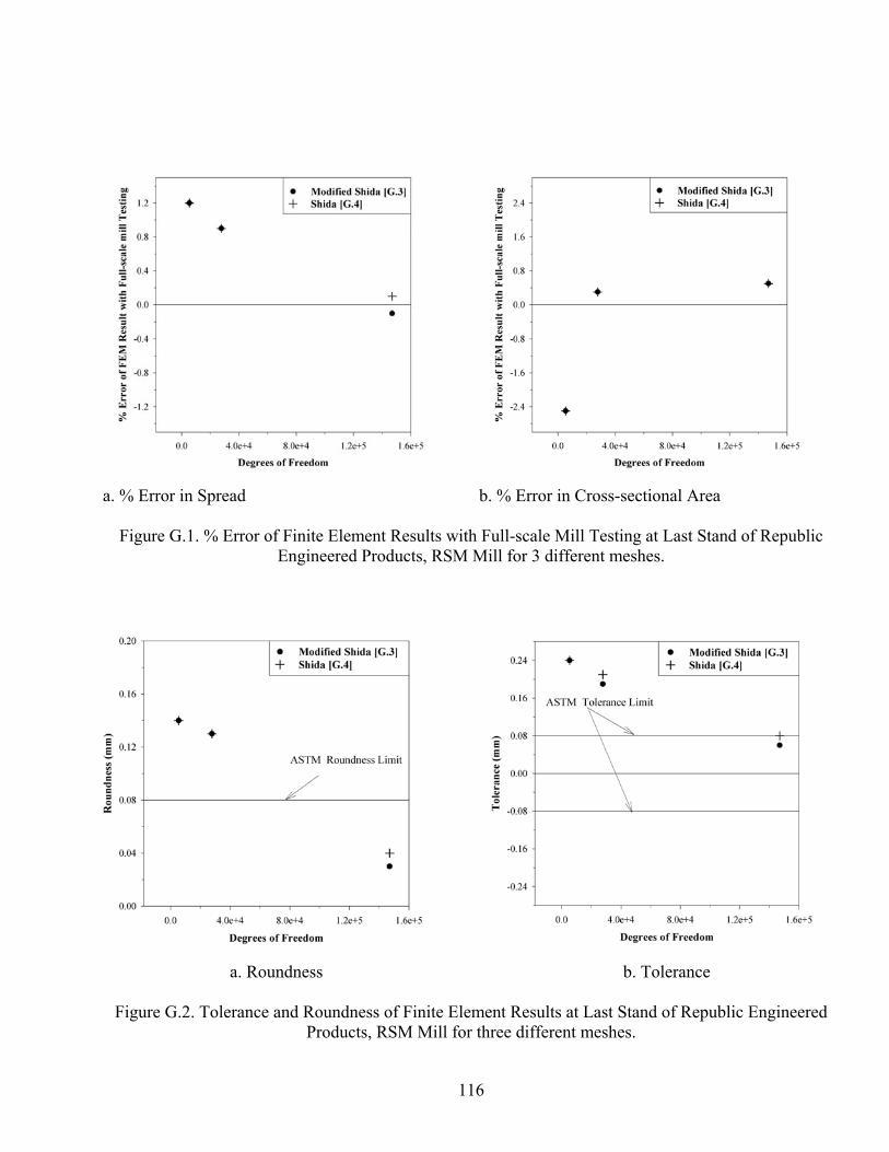
116
a. % Error in Spread b. % Error in Cross-sectional Area
Figure G.1. % Error of Finite Element Results with Full-scale Mill Testing at Last Stand of Republic Engineered Products, RSM Mill for 3 different meshes.
a. Roundness b. Tolerance
Figure G.2. Tolerance and Roundness of Finite Element Results at Last Stand of Republic Engineered Products, RSM Mill for three different meshes.

117
Appendix H: A New Approach for Theoretical Calculation of Stock Surface Profile in Multi-Stand Rolling
H.1. Overview
Theoretical calculation of surface profile is extremely important for accurately calculating of cross-sectional area, plastic strain and percentage reduction of stock in a multi-stand rolling process. Lee et al. [G.1] in 2000 proposed a model to calculate surface profile that is only valid for round-oval and oval-round passes. However, the model cannot be applied to two cases considered in this study. In these situations a commonly followed practice in industry is to assume the free surface as a straight line. In a large number of cases this assumption is also not accurate. In this chapter a more general approach to calculate stock surface profile is proposed. H.2. Proposed Approach
Figure H.1. Roll Groove surface and Stock Side Free Surface
In proposed approach the spread (w) is first calculated based on the method by Shinokura and Takai [G.2]. Then it is assumed that the rigid roll groove surface is represented by a curve ( )x f y= that is known. The side free surface is represented by the function ( )x g y= . The problem is assumed symmetric around X- and Y-axis and is therefore solved only for the first quadrant. Let Q (x1,y1) be the point where the roll groove surface ( ( )x f y= ) intersects the stock side free surface ( ( )x g y= ) and P (w/2,0) is the point of maximum width. The following assumptions are made regarding the free surface: -

118
1. The tangent to the free surface at point P is vertical, i.e., ,0
2
0wP
dgdy
=
2. The tangent to the free surface at point Q is collinear to tangent of the roll groove
surface at point Q i.e. ( ) ( )1 1 1 1, ,Q x y Q x y
df dgdy dy
=
3. The free surface is approximated as a complete quadratic polynomial as follows 2( )x g y Ay By C= = + + , where A, B and C are constants to be determined
Since point P is on the side free surface, it satisfies the equation 2( )x g y Ay By C= = + +
0 02w C= + +
yield, 2wC = (G.1a)
From assumptions 1 and 3, ( )/ 2,02 0
P wAy B+ =
yield, 0B = (G.1b) From assumptions 2 and 3, Equation G.1a and G.1b,
1 12 ( )Ay f y′= (G.1c) Since Q satisfies both ( )f y and ( )g y ,
21 1( )
2wAy f y+ = (G.1d)
Since ( )f y is a known function, unknowns A and 1y can be solved from Equations G.1c
& G.1d. Then the free surface curve can be written as 2( )2wx g y Ay= = + , where A is a
known constant. H.3. Advantages and Disadvantages The advantage of above-mentioned method is that theoretically it can be applied for any roll groove surface type. But the main drawback of this approach is it gives erroneous results for flat grooves since because in practice Assumption 2 is invalid for flat grooves. Further investigation is needed before this method can be applied universally for all stand sequence. Meanwhile this approach yields gives very accurate results for curved roll groove types that are commonly found.

119
Appendix I: Conference Paper This Paper Appear in the Following Conference:
1. Biswas, S., Rencis, J.J., Gutierrez, H. and Kiefer, B.V., User-oriented Three-dimensional Finite Element Modeling of High Speed Bar and Rod Rolling,To appear in the 45th Iron & Steel Society Mechanical Working and Steel Processing Conference, Chicago, IL, November 9-12, 2003.

120
User-Oriented Three-Dimensional Finite Element Modeling of High Speed
Bar and Rod Rolling
Souvik Biswas1, Joseph J. Rencis1, Horacio Gutierrez2, Bruce V. Kiefer2
1Mechanical Engineering Department; Worcester Polytechnic Institute; Worcester, MA 01609-2280
2Mill Process Modeling and Analysis; Morgan Construction Company; Worcester, MA 01605-2665
Keywords: Bar and Rod Rolling, Finite Element Analysis, Free Surface, High Speed
Rolling, Hot Rolling, Product Geometry, Rolling Simulation
Abstract A Java pre- and post-processing graphical user-oriented interface has been developed by the authors to aid a mill engineer with little or no finite element experience throughout the analysis process of the finishing rolling stands. A case study is presented that uses the commercial finite element code ABAQUS/Explicit to predict roundness and tolerance customer requirements. Other parameters that are determined include spread, cross-sectional area, percentage reduction in area, incremental plastic strain, total plastic strain and roll force. All parameters are compared to theoretical models and some are compared to full-scale mill testing.
Introduction to Case Study In this study a finite element model of the finishing rolling stands at a Morgan rolling mill is considered to produce a finished rod of AISI 1045 medium carbon steel with a 12.75 mm diameter. The customer (rod user) is a U.S. automotive supplier who will manufacturer M12 x 1.25, 4g (high accuracy, fine fits) steel bolt of SAE class 4.6 from the finished rod. The goal of the simulation is to produce a finished rod that will satisfy the automotive supplier requirements for roundness and tolerance in accordance to ASTM standards.
The details of the finishing rolling stands and incoming stock for the case study are first discussed. An overview of the user-oriented Java program developed by the authors for carrying out the ABAQUS finite element analysis by a mill engineer is then presented. Subsequent sections discuss the finite element model and how full-scale mill testing was carried out. The finite element results are then compared to theoretical and full-scale mill testing. The final section compares the finite element results, theoretical results and full-scale mill testing results with customer requirements.

121
Details of Finishing Rolling Stands and Incoming Stock The specifications of the finishing rolling stands and the incoming stock are defined in Table I. The geometric details regarding the finishing rolling stands were provided by Morgan. There are four finishing stands with a pass sequence of oval-round-round-round in the reducing/sizing (RSM) mill. Stand #1 consists of two oval grooved rolls and input stock is of circular cross-section. Stand #2 consists of two round grooved rolls oriented at 90o to the first stand and the output of Stand #1 is used as input stock for this stand. Stand #3 consists of two round grooved rolls oriented 90o to Stand #2 and the output of Stand #2 is used as input stock for this stand. Stand #4 consists of two round grooved rolls oriented 90o to Stand #3 and the output of Stand #3 is used as input stock for this stand.
Table I. Details of finishing rolling stands and incoming stock
FINISHING ROLLING STANDS INCOMING STOCK Pass Sequence Oval-round-round-round Translational Speed 19 m/s
Cross Section Profile 16.395 mm Diameter Stand Spacing (On-center)
Stands 1-2: 820 mm; Stands 2-3: 966 mm; Stands 3-4: 150 mm Section Length The stock is continuously
fed into the stands.
Roll Diameters
Stand #1: 211.09 mm; Stand #2: 211.09 mm; Stand #3: 145.13 mm; Stand #4: 145.14 mm
Material AISI 1045 Medium Carbon Steel
Roll Gaps
Stand #1: 1.2 mm; Stand #2: 1.36 mm; Stand #3: 1.32 mm; Stand #4: 1.4 mm
Chemical Composition C-0.45, Mn-0.75, P-0.04, S-0.05 (wt. %)
Roll Groove Geometries Defined by Morgan [1] Austenite Grain Size Not Applicable
Roll Material Tungsten Carbide
No-twist Rolling Stands are Alternatively Oriented 90o from Each
Other
Temperature Uniform at 910 oC
Roll Temperatures Not Applicable Strain Rate Range 350-500 s-1
Rotational Speed of Rolls Defined by Morgan [1] Specific Heat 475 J/Kg/K [2]
Roll/Stock Friction Friction due to contact between tungsten carbide roll and AISI 1045 stock surface with water present between as coolant.
Java Pre- and Post-processing Graphical User Interface A Java pre- and post-processing graphical user interface (GUI) was developed by the authors so that a mill engineer can define a finite element model of the mill setup. The long range goal is that the Java interface could be used by a mill engineer with little or no finite element experience. Using the analysis results the engineer can determine whether or not the mill setup satisfies customer requirements. The major reason why the Java language was selected is that it is platform independent; therefore, code does not have to be recompiled. The GUI was developed using the Java™ 2 Platform Standard Edition

122
[3]. The mill engineer uses the Java pre-processor program to define the finishing rolling stand and incoming stock. The groove geometry module of the Java pre-processor is shown in Figure 1. The mill engineer can input groove geometry data, stock geometry data, stock material property data, element and mesh information, boundary and initial conditions, stock/roll friction, temperature related data, etc. Once the stands and stock are defined, the pre-processor creates a Python script file. Through the ABAQUS/CAE interface the Python script file is used to automatically generate an input file (pre-processing stage) of the finite element model. The finite element model is then solved using the ABAQUS solver (processing stage). Once the finite element solution is complete, a Python script post-processor code is run from the ABAQUS/CAE command line to generate ASCII result files from the ABAQUS output database (In the future the plan is to integrate this process into the Java program so that the mill engineer does not have to carry it out manually.). The Java post-processor then reads the ASCII files and calculates geometric and deformation parameters that can be used to evaluate whether or not customer requirements are satisfied. An in-depth discussion of the Java pre- and post-processing program can be found in Souvik [4]. The mill engineer can also view the finite element results in ABAQUS/CAE or ABAQUS/Viewer.
Figure 1: Screen layout of the groove geometry module in the Java pre-processing program.
Finite Element Model The commercial finite element code ABAQUS/Explicit [5] version 6.3 was used in this work. Table II states the assumptions, solution techniques and other modeling parameters used in the finite element simulation of the four-stand reducing/sizing mill. The actual rolling stand configuration is shown in Figure 2 and the finite element model considered all four stands as shown in Figure 3. The three-dimensional hexahedral brick finite element model was considered transient using explicit time integration and is based on a Lagrangian formulation. A convergence study was carried out to determine the appropriate mesh size as discussed in Souvik [4]. The constitutive equation for

123
determining the flow stress of steel for different strain rates and temperature employed Lee [6] since the strain rate range in this work is 350-500 s-1 (Table I). Lee’s constitutive equation is valid for strain rate range of 1 s-1 to 3000 s-1 and is a modification of Shida [7] that has a strain range of 1 s-1 to 100 s-1. An in-depth review of the state-of-the-art for various experimental studies and empirical constitutive equations to predict flow stress behavior of steel at high temperature and strain rates can be found in Souvik [4].
Table II. Details of ABAQUS/Explicit finite element model for the incoming stock and rolling stands
Mesh Domain Lagrangian Time Dependence Transient
Time Integration Explicit, Dynamics, Adiabatic. Optimal time step is decided automatically by ABAQUS
Dimensionality Three-Dimensional Mass Scaling None
Adaptive Meshing Lagrangian Analysis: No
FORMULATION
Hourglass Artificial Stiffness Material Rigid
Finite Element Characterization Analytic Rigid Surface ROLL
Boundary Conditions Rotational Speed of Rolls (see Table I)
Element Type Linear Hexahedral Brick (C3D8R), Deformable, Reduced Integration
Mesh Characteristics # of Nodes: 49,994
# of Elements: 48,820 # of DOF: 147,030 (including Lagrange Multipliers)
Material Homogeneous and Isotropic Length 1.0 m1
Rate Dependence Yes Spring Back Calculation No
Plasticity Law Lee (Modified Shida)2 [6] Hardening Rate Isotropic
% Plastic Deformation Energy Converted to Heat 0.90 [8]
STOCK
Initial Conditions Initial Velocity of the Stock; Initial Temperature of the Stock
Contact Condition Tangential: Penalty; Normal: Hard
Friction Model Coulomb (µ=0.3) STOCK / ROLL
INTERFACE Heat Transfer Effects Not Applicable
Material Rigid Pin Support at Roll
Model Spacing (On-center)1 Stands 1-2: 250 mm; Stands 2-3: 200 mm; Stands 3-4: 200 mm STAND
Orientation3
Stand #1: Vertical; Stand #2: Horizontal;
Stand #3: Vertical; Stand #4: Horizontal
1The section length of the stock is kept 1.0 m in the finite element model to reduce the number of degrees of freedom. Inter stand distances are also minimized for the same reason.
2Appropriate models are being used based on the strain rates. 3Stand orientation for the finite element model was assumed oriented vertically and horizontally for simplicity in model
creation.

124
Figure 2: Actual rolling stand configuration. Figure 3: Finite element model of rolling stands.
Full-scale Mill Testing
A series of tests were conducted on one of Morgan’s RSM units installed in a rod production line in order to gather detailed dimensional data on the rolling stock for comparison with the finite element model and theoretical model in the next section. A standard size rod product of AISI 1045 carbon steel (Table I) was rolled in a series of tests in which the entry temperature to the RSM, the rolling rate and the entry dimensions were all held constant. The tests consisted of rolling a billet through four stands of the RSM to obtain rod samples.
Samples of the rolled product were obtained after the rod had passed through water cooling boxes, formed into continuous loops by the laying head and cooled on the air-cooling conveyor. Short samples were cut from the coils produced from each test. For dimensional measurement, the samples were placed in a custom-made system for detailed off-line dimensional measurements of rod and bar products using a laser gauge and specialized analysis software. Diameter measurements were obtained for sixty diametrical locations, giving a detailed representation of the stock geometry profile.
Results and Discussion The finite element solution is verified with theoretical models and validated with full-scale mill testing (see previous section). Table III summarizes the finite element, theoretical and full-scale mill testing results for spread, cross-sectional area, percentage reduction in area, incremental plastic strain, total plastic strain and roll force at all four stands. An in-depth review of the state-of-the-art theoretical and empirical geometric and deformation models for steel rod and bar round-oval and oval-round pass rolling can be found in Souvik [4].
The finite-element, theoretical, and full-scale mill testing results for the cross-sectional profile at Stands #1 through #4 are compared in Figure 4. Figures 5 compares the finite-

125
element and theoretical results for the incremental plastic strain and total plastic strain at Stands #1 through #4. Finite element plots of the cross-sectional plastic strain distribution at Stands #1 through #4 are shown in Figure 6. A comparison of the finite element model and theoretical model for the roll force at Stands #1 through #4 is shown in Figure 7.
Table III. Comparison of finite element, theoretical and full-scale mill testing results at each stand SPREAD (mm)
Method Stand #1 Stand #2 Stand #3 Stand #4
FEM 19.11 (-2.3%T)
13.58 (-0.9%T)
(-1.5%FST)
14.45 (3.1%T)
(3.0%FST)
12.81 (-0.2%T)
(-0.1%FST) Theoretical Lee [9]1 19.57 13.70 13.98 12.84
Full-scale Mill Testing - 14.01 14.02 12.82 CROSS-SECTIONAL AREA (mm2)
Method Stand #1 Stand #2 Stand #3 Stand #4
FEM 167.68 (-2.8%T)
145.72 (0.1%T)
(-0.6%FST)
134.92 (-0.7%T)
(0.2%FST)
128.84 (-1.3%T)
(0.5%FST) Theoretical Lee [9] 172.50 146.60 135.94 130.59
Full-scale Mill Testing - 145.66 134.66 128.15 PERCENTAGE REDUCTION IN AREA (%)
Method Stand #1 Stand #2 Stand #3 Stand #4
FEM 18.67 (2.1%T)
13.10 (-12.8%T)
7.40 (1.9 %T)
(-2.0%FST)
4.51 (14.5%T)
(-6.6%FST) Theoretical Lee [9] 18.28 15.02 7.27 3.94
Full-scale Mill Testing - - 7.55 4.83 INCREMENTAL PLASTIC STRAIN2 (mm/mm)
Method Stand #1 Stand #2 Stand #3 Stand #4
FEM 0.399 (5.2%T)
0.280 (-15.2%T)
0.107 (0.5%T)
0.081 (1.25%T)
Theoretical Lee [10]3 0.380 0.331 0.107 0.08
TOTAL PLASTIC STRAIN2 (mm/mm)
Method Stand #1 Stand #2 Stand #3 Stand #4
FEM 0.399 (5.2%T)
0.764 (7.6%T)
0.904 (11.2%T)
0.983 (13.1%T)
Theoretical Lee [10]3 0.380 0.710 0.814 0.869 ROLL FORCE (kN)
Method Stand #1 Stand #2 Stand #3 Stand #4
FEM 110.2 (-42.6%T)
80.7 (-48.3%T)
49.1 (7.7%T)
30.7 (20.5%T)
Theoretical Lee [11]4 191.9 156 46 26 T = % Difference with theoretical method. FST = % Difference with full-scale mill testing data. 1Spread factor β = 0.83. 2All strains are measured at exit of each stand. 3The theoretical strains are calculated by maximum width method [10]. 4Intersection between free surface and groove surface is approximated theoretically in absence of full-scale mill testing data.
Overall there is very good correlation between the finite element solution, theoretical solution and full-scale mill testing for spread and cross-sectional area of the stock. The percentage difference between finite element solution, theoretical solution and full-scale mill testing for spread and cross-sectional area is within 3% in the worst cases and in

126
most cases within 2%. It can be concluded that for last three stands with round grooves, the finite element solution for cross-sectional area is greater than full-scale mill testing cross-sectional area and less than theoretical cross-sectional area for all four stands.
There is no full-scale mill testing data available for incremental plastic strain and total plastic strain, therefore, only the theoretical and finite element solutions are compared. The theoretical and finite element solutions for incremental plastic strain and total plastic strain are consistent for the initial stands. However, the difference between them increases with successive stands due to error accumulation from the previous stands. Both the incremental plastic strain and total plastic strain finite element solution are generally greater than the theoretical solution and the percentage difference is within 15% in the worst case. However, the finite element solution is more useful than the theoretical solution since it determines the strain distribution that can be used to find mechanical properties and microstructure in future work.
There is no full-scale mill testing data available for roll force, therefore, only the theoretical and finite element solutions are compared. The finite element solution for roll force is less ≈40-50% of the theoretical solution for the first two stands where % reduction is large. This appears very large and is probably due to the fact that the actual model for calculating roll force by Lee [11] uses two parameters that are experimentally determined. In absence of experimental data these two parameters were determined theoretically. For the last two stands, where % reduction in area is small, the finite element solution for roll force is ≈10-20% greater than the theoretical solution. We have observed that the roll force obtained by the finite element solution is consistent and within ±10% of a proprietary Morgan model for evaluating roll force. The proprietary model employs a combination of empirical techniques that have been experimentally validated.
The results from Stand #4 (last stand) are very important, because the geometric tolerances and roundness at the stand exit determines part quality. There is a strong correlation between full-scale mill testing, finite element solution and theoretical solution for spread and cross-sectional area.

127
a. Stand #1. b. Stand #2.
c. Stand #3. d. Stand #4.
Figure 4: Cross-sectional profile and area for finite element, theoretical and full-scale mill testing for Stands #1 through #4.
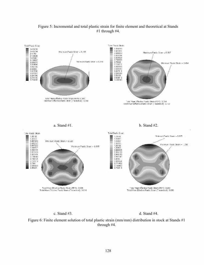
128
Figure 5: Incremental and total plastic strain for finite element and theoretical at Stands #1 through #4.
a. Stand #1. b. Stand #2.
c. Stand #3. d. Stand #4.
Figure 6: Finite element solution of total plastic strain (mm/mm) distribution in stock at Stands #1 through #4.
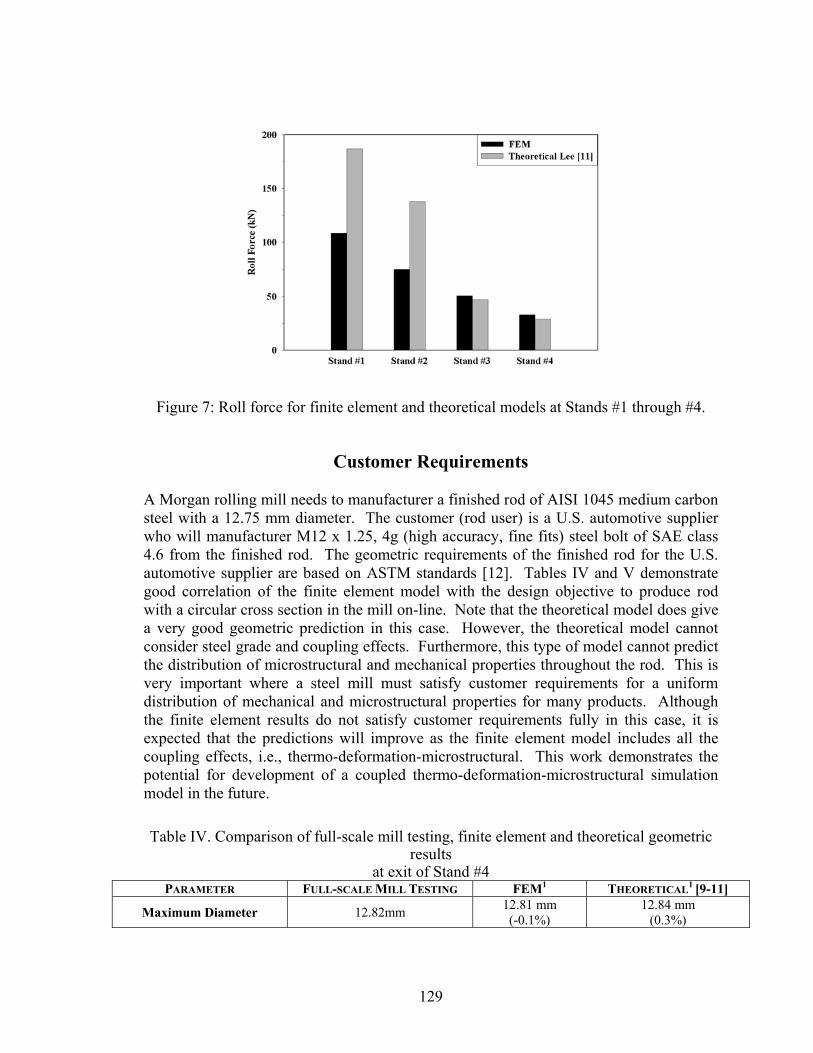
129
Figure 7: Roll force for finite element and theoretical models at Stands #1 through #4.
Customer Requirements A Morgan rolling mill needs to manufacturer a finished rod of AISI 1045 medium carbon steel with a 12.75 mm diameter. The customer (rod user) is a U.S. automotive supplier who will manufacturer M12 x 1.25, 4g (high accuracy, fine fits) steel bolt of SAE class 4.6 from the finished rod. The geometric requirements of the finished rod for the U.S. automotive supplier are based on ASTM standards [12]. Tables IV and V demonstrate good correlation of the finite element model with the design objective to produce rod with a circular cross section in the mill on-line. Note that the theoretical model does give a very good geometric prediction in this case. However, the theoretical model cannot consider steel grade and coupling effects. Furthermore, this type of model cannot predict the distribution of microstructural and mechanical properties throughout the rod. This is very important where a steel mill must satisfy customer requirements for a uniform distribution of mechanical and microstructural properties for many products. Although the finite element results do not satisfy customer requirements fully in this case, it is expected that the predictions will improve as the finite element model includes all the coupling effects, i.e., thermo-deformation-microstructural. This work demonstrates the potential for development of a coupled thermo-deformation-microstructural simulation model in the future.
Table IV. Comparison of full-scale mill testing, finite element and theoretical geometric
results at exit of Stand #4
PARAMETER FULL-SCALE MILL TESTING FEM1 THEORETICAL1 [9-11]
Maximum Diameter 12.82mm 12.81 mm (-0.1%)
12.84 mm (0.3%)

130
Minimum Diameter 12.75 mm 12.71 mm (-0.3%)
12.79 mm (0.3%)
Cross-sectional Area 128.15 mm2 128.84 mm2 (0.5%)
130.59 mm2 (1.9%)
1The quantity in parentheses represents the percentage difference between the parameter shown in the column and full-scale mill testing.

131
Table V. Geometry customer requirements and comparison with full-scale mill testing, finite element and theoretical model
ASTM REQUIREMENTS [12] FULL-SCALE MILL TESTING FEM THEORETICAL [9-11] Roundness1 0.08 mm 0.06 mm 0.1 mm 0.12 mm Tolerance2 + 0.08 mm + 0.07 mm + 0.06 mm +0.04 mm
1Roundness is the difference between maximum diameter and minimum diameter. 2Tolerance is the allowable difference in diameter between what a customer orders and what the steel mill delivers.
References
1. S.M. Shore, J. Dyck, and T.M. Shore, “New Rod Rolling Technology for Improved
Mill Utilization and Product Quality,” Metallurgical Plant and Technology International, August 1995, pp. 3-7.
2. MatWeb [Material Property Data], Automation Creations, Inc., 1996-2003,
http://www.matweb.com. 3. “Java 2 Platform, Standard Edition (J2SE),” Sun Microsystems Inc., 2003, Santa
Clara, CA, http://java.sun.com/j2se/downloads.html. 4. S. Biswas, “Simulation of Thermo-mechanical Deformation Evolution in High Speed
Rolling of Long Steel Products,” (M.S. Thesis, Mechanical Engineering Department, Worcester Polytechnic Institute, Worcester, MA, October, 2003).
5. ABAQUS/Explicit, ABAQUS, Inc. Corporate Headquarters, 1080 Main Street,
Pawtucket, RI, 2003, http://www.abaqus.com/. 6. Y. Lee, B.M. Kim, K.J. Park, S.W. Seo and O. Min, “A Study for the Constitutive
Equation of Carbon Steel Subjected to Large Strains, High Temperatures and High Strain Rates,” Journal of Materials Processing Technology, 130-131 (2002), 181-188.
7. S. Shida, “Effect of Carbon Content, Temperature and Strain Rate on Compressive
Flow Stress of Carbon Steels,” Hitachi Research Laboratory, 1974, p. 1. 8. S. Kobayashi, S. Oh, and T. Altan, Metal Forming and the Finite Element Method
(Oxford University Press, New York, 1989). 9. Y. Lee, S. Choi and Y.H. Kim, “Mathematical Model and Full-scale Mill Testing
Validation of Surface Profile of a Workpiece in Round-oval-round Pass Sequence,” Journal of Materials Processing Technology, 100 (2000), pp. 87-96.
10. Y. Lee, H.J. Kim, and S.M. Hwang, “Analytic Model for the Prediction of Mean
Effective Strain in Rod Rolling Process,” Journal of Materials Processing Technology, 114 (2001), 129-138.

132
11. Y. Lee and Y.H. Kim, “Approximate Analysis of Roll Force in a Round-oval-round Pass Rolling Sequence,” Journal of Materials Processing Technology, 113 (2001), 124-130.
12. “General Requirements for Wire Rods and Coarse Round Wire, Carbon Steel
[Metric],” ASTM A510M-82, Annual of ASTM Standards, (Philadelphia, PA: American Society for Testing and Materials, 1982), 314-321.
133
Appendix J: Thesis Presentation
Slide: 1
Simulation of Thermo-mechanical Deformation Evolution in High Speed Rolling of
Long Steel Products
M.S Thesis Presentationby
Souvik Biswas
Advisor: Prof. Joseph. J. Rencis
Slide: 2
Outline
• Motivation• Goal and Objectives • Introduction• Offline Simulation Process• Rolling Process Parameters and Theoretical Models• Two Case Studies• Conclusion• Future Work

134
Slide: 3
Motivation
• Tighter Tolerance Requirements by Customer• Unavailability of Offline Simulation Software to
US Steel Industry• Unavailability of FEM Simulation with Both
Deformation and Microstructure Evolution to US Steel Industry
• Increased International Competition
Slide: 4
Goal And Objectives
Goal:
Develop a Off-line Coupled Thermo-mechanical Finite Element Model for High Speed Hot Rolling
Objectives:
• Development of Thermo-mechanical Deformation Model• Verification and Validation of FEM Simulation Results• Development of a Simple User Friendly Graphical User
InterfacePre- and Post-ProcessingUsed by Mill Engineer with Little FEM experience

135
Slide: 5
Introduction
Major Parameters in Three Stages of Production
Why only Finishing Rolling Stage?• Entire Process Simulation too Costly
• Finishing Stage is Important for Product Quality
Slide: 6
Introduction
Rolling Parameters
Incoming Stock Incoming Stock
Finished Rod Finished Rod
Four Stand No-twist Finishing Block
Rod mill with a four Stand finishing block (Reducing Sizing Mill)

136
Slide: 7
Offline Simulation Process
Java Pre-processor
INPUT TO FEM FINISHING ROLLING MODELFinishing Rolling Stands Incoming Stock
Pass Sequence Translational SpeedStand Spacings Section Profile
Stand Stiffnesses Section LengthRoll Material Material
Roll Diameters Chemical CompositionRoll Gaps Austenite Grain Size
Roll Grove Geometries TemperatureNo-twist Rolling Stress-strain-Strain Rate DataRoll Temperature
Rotational Speed of RollsRoll/Stock Friction
Slide: 8
Offline Simulation Process
Heat FlowHeatingCooling
Variation ofThermo-physical
Properties
THREE-DIMENSIONAL FEM ROLLING MODEL
DeformationRolling Force and Torque
Flow StressStrain and Strain RateContact and Friction
TemperatureChemical Composition
Phases Present
MicrostructureChemical CompositionTemperature vs Time
% DeformationInitial Austenite Grain Size
Cooling ConditionsMicro ModelMicro Model
Macro Model
ABAQUS Processor

137
Slide: 9
Offline Simulation Process
OUTPUT FROM FEM ROLLING MODELGeometry Mechanical Properties Microstructure
Section Profile Yield Strength Grain SizeRoundness Ultimate Tensile Strength Grain Size DistributionTolerance % Reduction in Area Phase Composition
Hardness Phase Distribution
Java Post-Processor
Slide: 10
Offline Simulation Process
Java Pre-Processor
ABAQUS Processor
Java Post-Processor
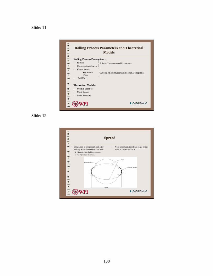
138
Slide: 11
Rolling Process Parameters and Theoretical Models
Rolling Process Parameters :• Spread• Cross-sectional Area• Plastic Strain
IncrementalTotal
• Roll Force
Theoretical Models:• Used in Practice• Most Recent• Most Accurate
Affects Tolerance and Roundness
Affects Microstructure and Material Properties
Slide: 12
Spread
• Dimension of Outgoing Stock after Rolling Stand in the Direction both
Normal to the Rolling directionCompression Direction
• Very important since final shape of the stock is dependent on it.
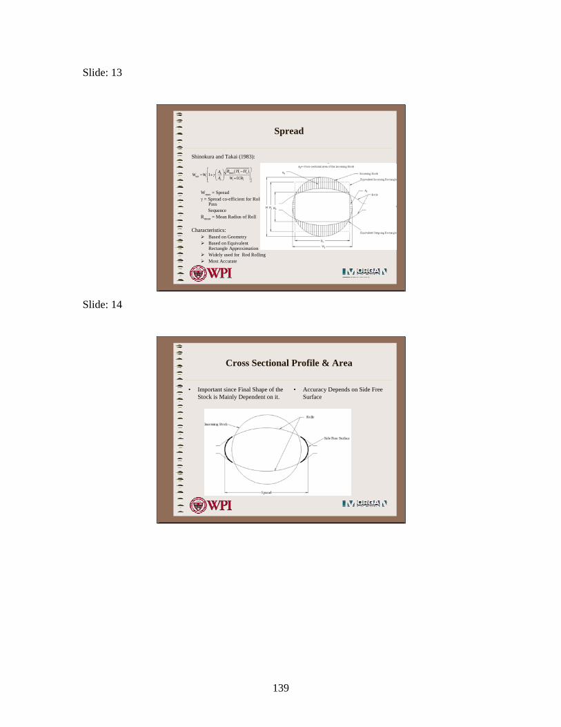
139
Slide: 13
Spread
Shinokura and Takai (1983):
Wmax = Spreadγ = Spread co-efficient for Roll
PassSequence
Rmean = Mean Radius of Roll
Characteristics:Based on GeometryBased on Equivalent Rectangle ApproximationWidely used for Rod RollingMost Accurate
( )max 1
0.5mean i oh
io i i
R H HAW WA W h
γ⎡ ⎤−⎛ ⎞⎢ ⎥= + ⎜ ⎟ +⎢ ⎥⎝ ⎠⎣ ⎦
Slide: 14
Cross Sectional Profile & Area
• Important since Final Shape of the Stock is Mainly Dependent on it.
• Accuracy Depends on Side Free Surface

140
Slide: 15
Cross Sectional Profile & Area
Side Free Surface Calculation• Oval-round and Round–oval
PassesLee et al. (2000)
Linear Interpolation between Groove Radius and Stock Radius using a Fraction based on Spread and Face WidthBased on GeometryOnce Free Surface is Obtained Cross-sectional Area is Calculated with Surface Profile
Slide: 16
Cross Sectional Profile & Area
Side Free Surface Calculation• Box and Square Passes
No method in LiteratureMorgan Proprietary
MethodAssumes Simple Shapes as ApproximationBased on years of Design ExperienceOnce Free Surface is Obtained Cross-sectional Area is Calculated with Surface Profile

141
Slide: 17
Plastic Strain
Plastic Strain: Due to Plastic Deformation in StockTypes of Plastic Strain:
– Incremental: Important for Calculation of Strain Rate– Total: Important for Calculation of Total Stain
Why Important?• Microstructure Evolution• Roll Force• Roll Torque • Power Requirements
Depends on Plastic Strain
Slide: 18
Incremental Plastic Strain
Incremental Plastic Strain: Maximum Average Equivalent Plastic Strain of Stock at a given Stand based on Incoming Stock Geometry and Outgoing Stock GeometryLee et al. (2000):
Hi = Initial Equivalent Height Ho = Final Equivalent Height Wi = Initial Equivalent Width Wo = Final Equivalent Width
Characteristics:– Based on Geometry– Assumes Equivalent Rectangle
Approximation of Stock Maximum Width Method
( )2 21 2 1 2
1
2
23
ln
ln
p
i
o
i
o
HHWW
ε ε ε ε ε
ε
ε
∆ = ∆ + ∆ + ∆ ∆
⎛ ⎞∆ = ⎜ ⎟⎝ ⎠⎛ ⎞∆ = ⎜ ⎟⎝ ⎠

142
Slide: 19
Total Plastic Strain
Total Plastic Strain : Maximum Average Equivalent Plastic Strain of Stock at a given Stand where Feed Section Geometry is InitialLee et al. (2000):
Hi = Initial Equivalent Height Ho = Final Equivalent Height Wi = Initial Equivalent Width Wo = Final Equivalent Width
Characteristics:– Based on Geometry– Assumes Equivalent Rectangle
Approximation Maximum Width Method
( )2 21 2 1 2
1
2
23
ln
ln
p
i
o
i
o
HHWW
ε ε ε ε ε
ε
ε
+= +
⎛ ⎞= ⎜ ⎟⎝ ⎠⎛ ⎞= ⎜ ⎟⎝ ⎠
Slide: 20
Roll Force
Roll Force: Force Acting on the Rolls in Direction of Compression
Why Important?• Roll Torque• Power Requirements
• Depends on Roll Force• Very Important in Roll Pass Design
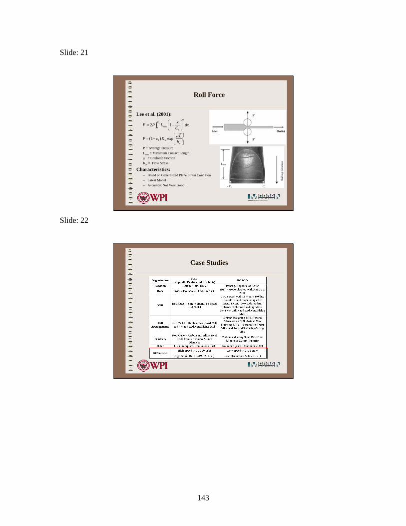
143
Slide: 21
Roll Force
Lee et al. (2001):
P = Average PressureLmax = Maximum Contact Lengthµ = Coulomb FrictionKm = Flow Stress
Characteristics:– Based on Generalized Plane Strain Condition– Latest Model– Accuracy: Not Very Good
( )
max0
1
2 1
1 exp
x
mC
x
mm
xF P L dxC
LP Khµε
⎛ ⎞= −⎜ ⎟
⎝ ⎠⎡ ⎤
= − ⎢ ⎥⎣ ⎦
∫
Slide: 22
Case Studies

144
Slide: 23
Case Study #1
• Republic Engineered Products RSM Mill, Lorain, OH
• Final Four Finishing Stands INLET
OUTLET
Slide: 24
Case Study #1
Actual Stands ABAQUS Finite Element Model
INLET
OUTLET

145
Slide: 25
Case Study #1 - ABAQUS FEM Modeling
Slide: 26
Case Study #1 - Material Constitutive Models
Modified Shida (Lee 2002)– Temperature Range: 25OC to 1000OC– Strain Rate Range: 1 s-1 to 3000 s-1
– Up to 1.2% Carbon Content– Validated with SHPB test (by Lee)
• 4340 Steel• 0.1% carbon Steel (0.1C-0.45Mn-0.25Si (wt%))• 0.72% carbon Steel (0.72C-0.45Mn-0.25Si (wt%))

146
Slide: 27
Results of Case Study #1- Spread
Shinokura and Takai (1983):
Results:– FEM, Theoretical and Full-scale
Testing are Consistent
( )max 1
0.5mean i oh
io i i
R H HAW WA W h
γ⎡ ⎤−⎛ ⎞⎢ ⎥= + ⎜ ⎟ +⎢ ⎥⎝ ⎠⎣ ⎦
Slide: 28
Results of Case Study #1- Cross Sectional Profile & Area
Stand #1 Stand #2 X (mm)
-10.0 -5.0 0.0 5.0 10.0
Y (m
m)
-10.0
-5.0
0.0
5.0
10.0FEMTheoretical Lee
AFEM = 167.68 mm2
AT = 172.50 mm2
X (mm)-10.0 -5.0 0.0 5.0 10.0
Y (m
m)
-10.0
-5.0
0.0
5.0
10.0FEMTheoretical LeeFull-scale Mill Testing
AFEM = 145.72 mm2
AT = 146.60 mm2
AFST = 145.66 mm2

147
Slide: 29
Results of Case Study #1- Cross Sectional Profile & Area
Stand #3
Stand #4.X (mm)
-10.0 -5.0 0.0 5.0 10.0
Y (m
m)
-10.0
-5.0
0.0
5.0
10.0FEMTheoretical LeeFull-scale Mill Testing
AFEM = 134.92 mm2
AT = 135.96 mm2
AFST = 134.66 mm2
X (mm)-10.0 -5.0 0.0 5.0 10.0
Y (m
m)
-10.0
-5.0
0.0
5.0
10.0FEMTheoretical LeeFull-scale Mill Testing
AFEM = 128.84 mm2
AT = 130.59 mm2
AFST = 128.15 mm2
•FEM, Theoretical and Full-scale Consistent•FEM is Generally Less than Theoretical
Slide: 30
Results of Case Study #1 – Incremental Plastic Strain
– FEM and Theoretical Consistent
Stand #0 Stand #1 Stand #2 Stand #3 Stand #4 Stand #
Plas
tic S
trai
n (m
m/m
m)
0.0
0.2
0.4
0.6
0.8
1.0Incremental:FEMIncremental:Theoretical Lee

148
Slide: 31
Results of Case Study #1 – Total Plastic Strain
– FEM and Theoretical Consistent
– Error Accumulation at Later Stands
Stand #0 Stand #1 Stand #2 Stand #3 Stand #4 Stand #
Plas
tic S
trai
n (m
m/m
m)
0.0
0.2
0.4
0.6
0.8
1.0
1.2
1.4 Incremental:FEMIncremental:Theoretical LeeTotal:FEMTotal:Theoretical Lee
Slide: 32
Results of Case Study #1 – Total Plastic Strain Distribution
Stand #1• FEM solution gives Strain distribution
Solution
Stand #2

149
Slide: 33
Results of Case Study #1 – Total Plastic Strain Distribution
Stand #3• FEM solution gives Strain distribution
Solution
Stand #4• Theoretical solution only gives
Average Strain
Slide: 34
Results of Case Study #1 – Roll Force
– Difference Between FEM and Theoretical AppearsVery Large
– Absence of Experimental Data: Two Experimental Parameters Approximated Theoretically
Stand #0 Stand #1 Stand #2 Stand #3 Stand #4 Stand #
Roll
Forc
e (k
N)
0
50
100
150
200FEMTheoretical Lee

150
Slide: 35
Results of Case Study #1 – Customer Requirements
Are Customer Requirements Satisfied?• Steel Manufacturer
• Customer– U.S. Automotive Supplier
• Product– M12 X 1.25, 4G Steel Bolt
• SAE Class 4.6• High Accuracy , Fine Fit Bolt
Slide: 36
Results of Case Study #1 – Customer Requirements
Roundness - Differences between maximum diameter and minimum diameterTolerance - Allowable difference in diameter between what a customer orders and what the steel mill delivers

151
Slide: 37
Case Study #1 – Mesh Convergence
Spread Cross-sectional Area
Degrees of Freedom
0.0 4.0e+4 8.0e+4 1.2e+5 1.6e+5
% E
rror
of
FEM
Res
ult
with
Ful
l-sca
le T
estin
g
-1.2
-0.8
-0.4
0.4
0.8
1.2
-0.0
Modified ShidaShida
Degrees of Freedom
0.0 4.0e+4 8.0e+4 1.2e+5 1.6e+5
% E
rror
of
FEM
Res
ult
with
Ful
l-sca
le T
estin
g
-2.4
-1.6
-0.8
0.8
1.6
2.4
-0.0
Modified ShidaShida
Slide: 38
Case Study #1 – Mesh Convergence
Roundness Tolerance
Degrees of Freedom
0.0 4.0e+4 8.0e+4 1.2e+5 1.6e+5
Roun
dnes
s (m
m)
0.00
0.08
0.16
0.24 Modified ShidaShida
Roundness Limit
Degrees of Freedom
0.0 4.0e+4 8.0e+4 1.2e+5 1.6e+5
Tole
ranc
e (m
m)
-0.24
-0.12
0.00
0.12
0.24Modified ShidaShida
Tolerance Limit

152
Slide: 39
Case Study #1 – Mesh Convergence
– Error between FEM and Full-scale Testing decreases with increase in number of degrees of freedom for both Spread and Cross-sectional
– FEM for roundness and tolerance improves with increase in number of degrees of freedom
– For the finest FE mesh considered solution actually satisfies ASTM standard for roundness and tolerance
Slide: 40
Case Study #2
• POSCO, No. 3 mill, Pohang, Korea • Initial Four Roughing Stands

153
Slide: 41
Case Study #2
Slide: 42
Results of Case Study #2 - Spread
Shinokura and Takai (1983):
Results:– FEM, Theoretical are Consistent
( )max 1
0.5mean i oh
io i i
R H HAW WA W h
γ⎡ ⎤−⎛ ⎞⎢ ⎥= + ⎜ ⎟ +⎢ ⎥⎝ ⎠⎣ ⎦

154
Slide: 43
Results of Case Study #2 - Cross Sectional Profile & Area
Stand #1 Stand #2 X (mm)
-100.0 -50.0 0.0 50.0 100.0
Y (m
m)
-100.0
-50.0
0.0
50.0
100.0FEMTheoretical Lee
AFEM = 20352.26 mm2
AT = 20828.64 mm2
X (mm)-100.0 -50.0 0.0 50.0 100.0
Y (m
m)
-100.0
-50.0
0.0
50.0
100.0
FEMTheoretical Lee
AFEM = 14440.42 mm2
AT = 14501.47 mm2
Slide: 44
Results of Case Study #2 - Cross Sectional Profile & Area
Stand #3. Stand #4.•FEM and Theoretical Consistent•FEM is Generally Less than Theoretical
X (mm)-100.0 -50.0 0.0 50.0 100.0
Y (m
m)
-100.0
-50.0
0.0
50.0
100.0FEMTheoretical Lee
AFEM = 10825.26 mm2
AT = 11142.66 mm2
X (mm)-100.0 -50.0 0.0 50.0 100.0
Y (m
m)
-100.0
-50.0
0.0
50.0
100.0FEMTheoretical Lee
AFEM = 8119.19 mm2
AT = 8328.73 mm2
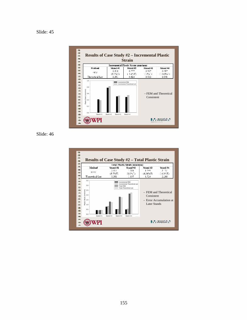
155
Slide: 45
Results of Case Study #2 – Incremental Plastic Strain
– FEM and Theoretical Consistent
Stand #0 Stand #1 Stand #2 Stand #3 Stand #4 Stand #
Plas
tic S
trai
n (m
m/m
m)
0.0
0.2
0.4
0.6
0.8
1.0Incremental:FEMIncremental:Theoretical Lee
Slide: 46
Results of Case Study #2 – Total Plastic Strain
– FEM and Theoretical Consistent
– Error Accumulation at Later Stands
Stand #0 Stand #1 Stand #2 Stand #3 Stand #4 Stand #
Plas
tic S
trai
n (m
m/m
m)
0.0
0.5
1.0
1.5
2.0
2.5
3.0
3.5Incremental:FEMIncremental:Theoretical LeeTotal:FEMTotal:Theoretical Lee

156
Slide: 47
Results of Case Study #2 – Total Plastic Strain Distribution
Stand #1• FEM solution gives Strain
distribution Solution
Stand #2
Slide: 48
Results of Case Study #2 – Total Plastic Strain Distribution
Stand #3• FEM solution gives Strain distribution
Solution
Stand #4

157
Slide: 49
Results of Case Study #2 – Roll Force
– Difference Between FEM and Theoretical AppearsVery Large
– Absence of Experimental Data: Two Experimental Parameters Approximated Theoretically
Stand #0 Stand #1 Stand #2 Stand #3 Stand #4 Stand #5
Roll
Forc
e (k
N)
0
1000
2000
3000
4000
5000FEMTheoretical Lee
Slide: 50
Conclusion
• Validates the ABAQUS/Explicit Lagrangian/ALE FEM model to simulate 3-dimensional Rolling for a wide range of rolling speeds and strain rates
• FEM solution for Geometrical/Deformation parameters are Highly consistent with Theoretical and Full-scale Mill testing
• FEM Simulation Approach can be used for Roll-Pass Design• JAVA-GUI Pre- and Post- Processor can be used by a Mill engineer
with no FEM Background

158
Slide: 51
Future Work
• Theoretical Calculation of Stock Temperature during Rolling Process • Microstructure Evolution of Stock During Rolling Process• Improvements to Java Pre- and Post- Processor • Improvements to Finite Element Model• Improvement of Theoretical-Empirical Model Based on Numerical
Experiments
Slide: 52
Acknowledgements

159
Slide: 53
Questions?