Embed Size (px)
Citation preview

Simulation of Process Control Network Traffic
Viktor Andersson Tommi Nylander
Department of Automatic Control

Msc Thesis ISRN LUTFD2/TFRT--5949--SE ISSN 0280-5316
Department of Automatic Control Lund University Box 118 SE-221 00 LUND Sweden
© 2014 by Viktor Andersson & Tommi Nylander. All rights reserved. Printed in Sweden by Media-Tryck Lund 2014

Abstract
The majority of industrial control systems today are distributed over networks.These systems tend to be complex, and can be difficult both to configure and toanalyze; therefore, there is definitely a gain in being able to simulate the behaviourof such a system prior to the actual implementation.
This master’s thesis investigates the possibility to simulate the ABB automationsystem 800xA by expanding the Matlab/Simulink tool TrueTime. Throughout, thework has been focused on modeling the network communications and the internalbehaviour of the control system nodes. Furthermore, the developed simulator hasbeen used to examine a proposal to optimize traffic handling of the ABB specificprotocol IAC.
Different performance measures have been investigated, both regarding control andnetwork performance. One measure of particular interest has been the round triptime of a packet. The simulator has proven to be able to reproduce results of roundtrip times measured in an example system, explaining timing behaviour originatingdeep down in the control system nodes. Other simulations have involved differentsystem settings, analyzing their impact on system performance.
i


Acknowledgements
We would like to express our special appreciation to our supervisor SvengunnarTiljander for his constant support during our time at ABB. Also, we would like tothank Adam Norén for his curiosity in our master’s thesis and his ideas and helpregarding the optimization of IAC traffic handling. For practical matters, AndreasEkstrand has helped us and furthermore he presented the opportunity of doing themaster’s thesis at ABB to begin with. Prof. Karl-Erik Årzén, our representative atLTH, has given much valuable ideas for the report.
iii


Contents
1. Introduction 11.1 Background . . . . . . . . . . . . . . . . . . . . . . . . . . . . 11.2 Goals . . . . . . . . . . . . . . . . . . . . . . . . . . . . . . . . 11.3 Individual Contributions . . . . . . . . . . . . . . . . . . . . . . 21.4 Outline . . . . . . . . . . . . . . . . . . . . . . . . . . . . . . . 3
2. Overview of the 800xA System 42.1 Usage . . . . . . . . . . . . . . . . . . . . . . . . . . . . . . . 42.2 Hardware . . . . . . . . . . . . . . . . . . . . . . . . . . . . . . 52.3 Software . . . . . . . . . . . . . . . . . . . . . . . . . . . . . . 6
3. Network Structure in 800xA 103.1 Protocols used in 800xA . . . . . . . . . . . . . . . . . . . . . . 123.2 Switched Ethernet . . . . . . . . . . . . . . . . . . . . . . . . . 123.3 RNRP - Redundant Network Routing Protocol . . . . . . . . . . 143.4 UDP - User Datagram Protocol . . . . . . . . . . . . . . . . . . 163.5 TCP - Transmission Control Protocol . . . . . . . . . . . . . . . 163.6 IAC - Inter Application Communication . . . . . . . . . . . . . 233.7 MMS - Manufacturing Message Specification . . . . . . . . . . 25
4. Simulation of Real Time Network Distributed Systems 264.1 Simulation Tool Alternatives . . . . . . . . . . . . . . . . . . . 264.2 TrueTime . . . . . . . . . . . . . . . . . . . . . . . . . . . . . . 28
5. Modeling and Simulation of 800xA 355.1 Helper File . . . . . . . . . . . . . . . . . . . . . . . . . . . . . 355.2 Implementation in TrueTime . . . . . . . . . . . . . . . . . . . 355.3 Simulating RNRP with TrueTime . . . . . . . . . . . . . . . . . 385.4 Simulating TCP with TrueTime . . . . . . . . . . . . . . . . . . 425.5 Simulating IAC with TrueTime . . . . . . . . . . . . . . . . . . 475.6 Simulating MMS with TrueTime . . . . . . . . . . . . . . . . . 50
6. Results of TrueTime Simulations 536.1 Sensor/Actuator - Regulator Example . . . . . . . . . . . . . . . 53
v

Contents
6.2 Measuring Performance . . . . . . . . . . . . . . . . . . . . . . 566.3 Handling of Packet Losses . . . . . . . . . . . . . . . . . . . . . 606.4 Investigating RNRP Settings . . . . . . . . . . . . . . . . . . . 62
7. Optimization of IAC traffic 677.1 The Current Implementation . . . . . . . . . . . . . . . . . . . . 677.2 The Proposed Optimization . . . . . . . . . . . . . . . . . . . . 687.3 When Are Faster Round Trip Times Beneficial? . . . . . . . . . 70
8. Results and Validation of IAC Optimization 718.1 Measurement Results . . . . . . . . . . . . . . . . . . . . . . . 718.2 Simulation Accuracy . . . . . . . . . . . . . . . . . . . . . . . 778.3 Comparison to Current Implementation . . . . . . . . . . . . . . 87
9. Conclusions 899.1 Using TrueTime to Model 800xA . . . . . . . . . . . . . . . . . 899.2 Optimizing IAC Traffic . . . . . . . . . . . . . . . . . . . . . . 899.3 Future Work . . . . . . . . . . . . . . . . . . . . . . . . . . . . 90
Bibliography 92
vi

List of Figures
2.1 AC 800M controller . . . . . . . . . . . . . . . . . . . . . . . . . . . 62.2 800xA operation station . . . . . . . . . . . . . . . . . . . . . . . . . 82.3 Project in Control Builder . . . . . . . . . . . . . . . . . . . . . . . . 9
3.1 800xA network overview . . . . . . . . . . . . . . . . . . . . . . . . 113.2 OSI model . . . . . . . . . . . . . . . . . . . . . . . . . . . . . . . . 133.3 Switched Ethernet . . . . . . . . . . . . . . . . . . . . . . . . . . . . 143.4 RNRP network topology . . . . . . . . . . . . . . . . . . . . . . . . 153.5 UDP header . . . . . . . . . . . . . . . . . . . . . . . . . . . . . . . 163.6 TCP header . . . . . . . . . . . . . . . . . . . . . . . . . . . . . . . 173.7 TCP connection establishment and termination . . . . . . . . . . . . 183.8 The TCP send window . . . . . . . . . . . . . . . . . . . . . . . . . 193.9 TCP error control . . . . . . . . . . . . . . . . . . . . . . . . . . . . 213.10 TCP congestion control . . . . . . . . . . . . . . . . . . . . . . . . . 233.11 IAC client . . . . . . . . . . . . . . . . . . . . . . . . . . . . . . . . 243.12 IAC server . . . . . . . . . . . . . . . . . . . . . . . . . . . . . . . . 243.13 MMS variable value exchange . . . . . . . . . . . . . . . . . . . . . 25
4.1 The TrueTime block library . . . . . . . . . . . . . . . . . . . . . . . 294.2 Network Schedule in Raw Form . . . . . . . . . . . . . . . . . . . . 314.3 RTSys class overview . . . . . . . . . . . . . . . . . . . . . . . . . . 33
5.1 Class overview of the protocol_helper.cpp file . . . . . . . . . . 365.2 Packet class structure . . . . . . . . . . . . . . . . . . . . . . . . . . 395.3 RNRP forwarding logic . . . . . . . . . . . . . . . . . . . . . . . . . 415.4 TcpConnection class overview . . . . . . . . . . . . . . . . . . . . . 435.5 IacHandler class overview . . . . . . . . . . . . . . . . . . . . . . . 50
6.1 Regulator example . . . . . . . . . . . . . . . . . . . . . . . . . . . 546.2 Smooth network utilization . . . . . . . . . . . . . . . . . . . . . . . 596.3 MMS versus IAC with 10 % loss probability . . . . . . . . . . . . . . 62
vii

6.4 RNRP redirecting network traffic . . . . . . . . . . . . . . . . . . . . 636.5 Network schedules when RNRP is redirecting network traffic . . . . . 646.6 Simulation of experiment when number of allowed hello packets lost is
set to 0 . . . . . . . . . . . . . . . . . . . . . . . . . . . . . . . . . . 65
7.1 Threads in current IAC implementation . . . . . . . . . . . . . . . . 687.2 Threads in filtered IAC implementation . . . . . . . . . . . . . . . . 69
8.1 Measured RTTs with default firmware - 5 IAC and 50 MMS . . . . . 728.2 Histogram of measured RTTs with default firmware - 5 IAC and 50
MMS . . . . . . . . . . . . . . . . . . . . . . . . . . . . . . . . . . 728.3 Measured RTTs with optimized firmware - 5 IAC and 50 MMS . . . . 738.4 Histogram of measured RTTs with optimized firmware - 5 IAC and 50
MMS . . . . . . . . . . . . . . . . . . . . . . . . . . . . . . . . . . 738.5 Measured RTTs with default firmware - 5 IAC . . . . . . . . . . . . . 748.6 Histogram of measured RTTs with default firmware - 5 IAC . . . . . 748.7 Measured RTTs with optimized firmware - 5 IAC . . . . . . . . . . . 758.8 Histogram of measured RTTs with optimized firmware - 5 IAC . . . . 758.9 New measurement of RTTs with optimized firmware - 5 IAC . . . . . 768.10 Histogram of newly measured RTTs with optimized firmware - 5 IAC 768.11 Simulation RTTs before model adjustment . . . . . . . . . . . . . . . 778.12 Difference between measured and actual RTTs . . . . . . . . . . . . 788.13 Protocol handler timing explained - case 1 . . . . . . . . . . . . . . . 808.14 Protocol handler timing explained - case 2 . . . . . . . . . . . . . . . 818.15 Protocol handler timing explained - case 3 . . . . . . . . . . . . . . . 828.16 Protocol handler timing explained - case 4 . . . . . . . . . . . . . . . 838.17 Simulated RTTs - case 1 . . . . . . . . . . . . . . . . . . . . . . . . 848.18 Simulated RTTs - case 1, no interfering tasks . . . . . . . . . . . . . 848.19 Simulated RTTs - case 2 . . . . . . . . . . . . . . . . . . . . . . . . 858.20 Simulated RTTs - case 3 . . . . . . . . . . . . . . . . . . . . . . . . 868.21 Simulated RTTs - case 4 . . . . . . . . . . . . . . . . . . . . . . . . 868.22 Simulated RTTs with filtered IAC implementation - case 1 . . . . . . 878.23 Simulated RTTs with filtered IAC implementation - case 2 . . . . . . 88
viii

List of Tables
List of Tables
6.1 PID settings . . . . . . . . . . . . . . . . . . . . . . . . . . . . . . . 566.2 Performance measures comparing MMS and IAC protocols . . . . . . 61
7.1 Performance measures for studying the impact of optimized RTTs . . 70
ix
Abbreviations
ABB Asea Brown Boveri
ACK Acknowledgement
CA Congestion Avoidance
CAN Controller Area Network
CNCP Control Network Clock Protocol
CSMA/AMPCarrier Sense Multiple Access with Arbitrationon Message Priority
CSMA/CDCarrier Sense Multiple Access with CollisionDetection
cwnd Congestion Window
DES Discrete Event Simulation
FBD Function Block Diagram
FDMA Frequency Division Multiple Access
FIN Final
FR Fast Recovery
HMI Human Machine Interface
IAC Inter Application Communication
IAE Integral Absolute Error
IL Instruction List
I/O Input/Output
ISE Integral Squared Error
x

List of Tables
ITAE Intergral Time Absolute Error
IP Internet Protocol
LAN Local Area Network
LD Ladder Diagram
MMS Manufacturing Message Specification
MSL Maximum Segment Lifetime
MSS Maximum Segment Size
OSI Open Systems Interconnection
PID Proportional Integral Derivative
PLC Progammable Logic Controller
PPP Point-to-Point Protocol
RNRP Redundant Network Routing Protocol
RTO Retransmission Time-Out
RTT Round Trip Time
SEQ Sequence Number
SFC Sequential Function Chart
SIL Safety Integrity Level
SNTP Simple Network Time Protocol
SS Slow Start
ssthresh Slow Start Threshold
ST Structured Text
SYN Syncronised
TCP Transmission Control Protocol
TDMA Time Division Multiple Access
UDP User Datagram Protocol
xi


1Introduction
This master’s thesis covers simulation of the network structure of the ABB controlsystem 800xA, and what improvements that could be implemented using the results.The thesis is collaboration between ABB and the Department of Automatic Control,Lund University, where the simulation tool, TrueTime, utilized in this project wasdeveloped. The work was performed at ABB Business Center, Malmö.
1.1 Background
Modern control systems are to an increasing degree distributed over networks. Ex-amples include control systems in large factories, oil rigs, air planes and cloud basedcontrol systems. These kinds of distributed systems tend to be very complex, andthe task of analyzing and predicting the outcome of such systems is far from triv-ial, not to mention how difficult it can be to develop the systems. Hence, an effortto simulate the systems can be worth a try, as the simulation greatly can simplifysystem implementation and analysis. If successful, the simulation also lets the userexperiment with different settings much faster and easier than in reality. Also, it canhelp the user to understand the behaviour of the system and could for instance beused for discovering ways to optimize the system.
1.2 Goals
The goal of this thesis is to model and simulate the 800xA distributed control systemdeveloped at ABB. In order to speed up development, a simulation tool TrueTimehas been used. This is a Matlab/Simulink based tool, developed at the Departmentof Automatic Control at LTH, and works as a framework for our implementation.TrueTime is designed to simulate real time systems in general but has the feature ofmodeling networks in the system, at least for low level protocols. Also, the integra-tion with Matlab/Simulink makes TrueTime ideal for simulating control systemsacting on (simulated) physical processes. Though, the question remained, couldTrueTime be used, in the way described above, to simulate the 800xA distributed
1

Chapter 1. Introduction
control system?
This master’s thesis started as a study in the simulation of the 800xA system only,but as time passed it also became an investigation of how the simulation could bevalidated and put to use. This finally led the thesis in the direction of studying theso called round trip times, i.e. the time it takes to get an answer to a request, when anetwork node reads a value from another unit. Especially, the details of the sendingand receiving mechanisms of the system were studied and the simulated results werecompared to those obtained from measurements of a real system. Furthermore, thegained knowledge from the simulation was utilized in an attempt to optimize thepacket path in the system, with the intention of shortening the round trip times;thus, improving system performance.
1.3 Individual Contributions
This master’s thesis has above all been focusing on implementation and most of thetime has been spent on discussing and coming up with solutions. Thus, a majorityof the work has been done together. However, Tommi’s previous experience fromdata communication and networks has proven very valuable, especially when im-plementing the simulated TCP protocol. Viktor has been in charge of the overallstructure and object oriented design of the program. Also, he has been responsiblefor the graphics used in the report. Furthermore, both authors have been involved inall phases of the thesis, from implementation to writing the report.
2

1.4 Outline
1.4 Outline
An introduction to the ABB control system 800xA is provided, focusing on thecomponents involved and the system’s application areas is presented in Chapter 2- Overview of the 800xA System. In Chapter 3 - Network Structure in 800xA, theoverall network structure of 800xA is described, and important protocols on the net-work, transport and application layer are presented and explained thoroughly. Fur-thermore, Chapter 4 - Simulation of Real Time Network Distributed Systems coversthe principles of network simulators. Also, the main simulation tool utilized in thisthesis, TrueTime, is described in depth, and other alternatives are presented as well.Chapter 5 - Modeling and Simulation of 800xA describes implementation detailsof the simulation and modeling. This chapter follows Chapter 3 to a great extent,mapping theory to implementation. The use of the 800xA simulator is demonstratedin Chapter 6 - Results of TrueTime Simulations. This chapter also shows differentscenarios that have been investigated. The current implementation of handling IACtraffic in the automation system is presented in Chapter 7 - Optimization of IACtraffic, and an optimized alternative is proposed with simulation results as back-ground.In Chapter 8 - Results and Validation of IAC Optimization, the results ofthe optimized IAC implementation are discussed and compared to the simulations.The results of this project are evaluated and conclusions are drawn in Chapter 9 -Conclusions. Also, possible future work is proposed.
3

2Overview of the 800xASystem
The ABB 800xA system is a highly customizable automation system with focus onintegration and safety. 800xA consists of several hardware and software componentsthat together form the system. Covering this vast automation system completely isnot possible, however, this chapter gives a brief overview and particularly presentsthe parts important to the thesis.
2.1 Usage
The 800xA system is used all over the world in larger facilities such as:
• factories
• dairy industry
• paper industry
• oil rigs
• nuclear power plants
• water dams
In general the 800xA system is used in process industry, especially in safety criticalapplications. To ensure the users a safe system, 800xA is SIL (Safety IntegrityLevel) classified at level 3, which means that the system has passed certain testsand that the system has been developed in a safe manner. For instance, if somethinggoes wrong in a nuclear power plant, it is absolutely crucial that the automationsystem works properly.
4

2.2 Hardware
In process industry, one is often controlling processes of a slow nature, and it is oftenmore important to stay close to reference values during disturbances than being ableto quickly follow a reference change. The actual physical process controlled couldbe almost anything, examples include:
• fluid levels in tanks
• heat in ovens
• pressure in gas/fluid containers
• flow of gases/fluids
• positions/velocities/forces in mechanical systems
• voltage
• biological processes
• chemical processes
• speed of conveyor belts
This has been taking into consideration in the simulations done in the thesis.
2.2 Hardware
The most important hardware units that make up the 800xA system are the con-trollers and I/O modules.
AC 800M controllersThe core of the 800xA system are the controllers, that is, the PLC processingunits that receive measurement signals and calculate what to do in the system.The controllers utilized in this master’s thesis are the AC 800M controllers, morespecifically with main unit type PM861A.
There are eight different main CPU models in the AC 800M family, with varyingspecifications and features including SIL-rating and redundancy support. The units’clock frequencies (24-450 MHz) and RAM (8-256 MB) are small in comparisonwith a standard PC. The main unit used in this master’s thesis, the PM861A, hasa clock frequency of 48 MHz, 16 MB RAM, a flash memory slot and CPU redun-dancy support [ABB, 2013c].
SIL-3 certification is obtained by the unit PM865A, and is by ABB called a tex-titHigh Integrity (HI) controller. It can be extended by a safety module SM811 that
5

Chapter 2. Overview of the 800xA System
runs all calculations in parallel with the main unit. This way the precision and relia-bility of the controller are greatly enhanced. This configuration of the units enablesfor both safety critical and standard process automation applications. It is also pos-sible to attach and interconnect other units to all AC 800M main units, includingI/O modules and fieldbuses, which are described later on in this section. See Figure2.1 for a small High Integrity AC 800M set up.
Figure 2.1 An AC 800M controller set up, here with a main unit PM865A (second left-most), with attached safety module (leftmost) and two I/O modules (to the right).
In an AC 800M controller a lot of different threads are running. Later in the report acloser look will be taken at some of them. The threads that are of particular interestare the ones handling network traffic and the ones that takes care of packets. Theother threads will in the simulation be seen as interfering threads in the controller[System 800xA 5.1, Product Catalog (FP4 included), p. 5].
I/O ModulesThe I/O modules of 800xA can both act as extensions to the AC 800M controllers,or be part of a distributed process I/O system that communicates with parent con-trollers over fieldbuses. As simple extensions, the I/O modules take care of theinterface between AC 800M main unit and the input and output signals. However,on their own they also form the I/O systems S800 I/O and S900 I/O. These systemspermit installation in the field, close to the sensors and actuators. This reduces thecost of cabling and is also useful for installations in hazardous areas [ABB, 2013d].
2.3 Software
The most important component in the 800xA automation system is perhaps thesoftware, which enables the user to both create the control logic executed in thehardware and to supervise the processes.
6

2.3 Software
Process Portal AThe main tool that handles and configures settings related to the control applicationsis the Process Portal A (PPA). In this tool, the user can specify everything from userprofiles to included hardware/software libraries, and manage the projects created inthe Control Builder tool.
Control BuilderThe Control Builder is a software tool developed for building applications in thecontrol system. It is possible to create applications that run on the controllers, defin-ing the logic and tasks.
The controller applications are created in projects, where all necessary componentsare available for configuration. See Figure 2.3 for an overview of a typical project.The main included parts are:
• libraries
• applications
• controllers
The Libraries concern both the software and the hardware. In the former case, thesoftware libraries define e.g. data types, function blocks and control module types.When a software library is included in a project, these types become available in theapplications. The hardware libraries define code closer to the hardware and the corefunctionality of the controller. An example is the protocol handler, part of BasicH-wLib, which defines the controller communication handling.The Applications contain the actual controller logic and are connected to tasks thatexecute on the controllers. The code is written in programs or diagrams. In thismaster’s thesis, programs have been used exclusively. In the programs it is possibleto declare and set variables, communication variables and function blocks. The codecan be written in 5 different languages, defined by the IEC-61131 standard [ABB,2006, p. 158]:
• Instruction List (IL)
• Ladder Diagram (LD)
• Function Block Diagram (FBD)
• Sequential Function Chart (SFC)
• Structured Text (ST)
7

Chapter 2. Overview of the 800xA System
IL resembles assembly code, whereas LD, FBD and SFC are graphical languages.ST is a function oriented text based language, and is the only language utilized inthe simple programs created in this master’s thesis.The Controllers define the hardware that the applications run on. It is possible toconfigure the network settings of the units, including the IP address of the con-trollers, and other hardware related settings as well. Tasks are created in each con-troller, and assigned e.g. priorities and period times. These tasks are then connectedto the programs and applications, to define how they should run in the controller.
Operator StationsThe 800xA system also includes software for operator stations, which are completeHMI (Human Machine Interface) environments where plant operators can get anoverview of the system status. The software provides the possibility to control thesystem remotely and take actions if needed. See Figure 2.2 for an example of atypical 800xA operator station.
Figure 2.2 A typical 800xA operator station.
8

2.3 Software
Figure 2.3 A project in the Control Builder software.9

3Network Structure in 800xA
The network in an 800xA system can be seen as four different parts: the plantnetwork, the client/server network, the controller network and the fieldbus/fieldnetwork. This master’s thesis focuses on the communication in the controller net-work, but to understand the system, at least some basic knowledge about the othernetworks is needed.
In the plant network, so called thin clients can connect to the system and are typi-cally used for monitoring the system. The thin clients cannot access the rest of thenetwork directly, they are isolated through an isolation device as seen in Figure 3.1.From this isolation device the thin clients can get data from the system.
The client/server network is used for communication between workplaces(clients)/server and server/server. The servers are called connectivity servers andhandle the separation and communication between the different networks. To clar-ify, the client/server networks can communicate with the control network throughthe connectivity server(s). The workplaces, or clients, are used by the plant opera-tors [ABB, 2012, p.22-24].
In the control network, all communication between the controllers is made. Also,the communication between controllers and connectivity servers is done in thecontrol network. It is possible to include workplaces in the control network but it isalmost never done in practice, since this can cause performance issues. However, insome rare cases when using a small system, it can be sufficient.
The fieldbus/field network is used for communication with modules in the plant,e.g. I/O units. These modules can communicate either directly with a controlleror via a connectivity server [ABB, 2012, p.22-24]. 800xA supports third partyfield buses such as PROFIBUS, PROFINET, FOUNDATION Fieldbus, HART andMODBUS TCP [ABB, 2013b].
10

Chapter 3. Network Structure in 800xA
Figure 3.1 An overview of the 800xA network topology. Inspired by [ABB, 2012, p. 22].
Both the client/server network and the control network have the feature of usingredundant networks, i.e. one primary network and one secondary for backup. Thisis used when extra robustness is wanted for the system. The network redundancyis managed by the RNRP (Redundant Network Routing Protocol) protocol [ABB,2012, p.28].
11

Chapter 3. Network Structure in 800xA
3.1 Protocols used in 800xA
The AC 800M controllers and connectivity servers in the network can communicateusing the following protocols:
• Application Layer Protocols
– MMS - Manufacturing Message Specification
– IAC - Inter Application Communication
– SNTP - Simple Network Time Protocol
– CNCP - Control Network Clocl Protocol
• Transport Layer Protocols
– TCP - Transmission Control Protocol
– UDP - User Datagram Protocol
• Network Layer Protocols
– RNRP - Redundant Network Routing Protocol
• Link Layer Protocols
– Switched Ethernet
– PPP - Point-to-Point Protocol
Here, the different layers are the ones defined in the standard OSI (Open SystemsInterconnection) model. That is, a model that divides a network into seven differ-ent layers: Application, Presentation, Session, Transport, Network, Data Link andPhysical, as seen to the left in Figure 3.2. Read more about the OSI model at [TheOSI Model’s Seven Layers Defined and Functions Explained 2014].
All protocols relevant to this project are described in the following sections. TheCNCP and SNTP protocols are used for time synchronization in the system. Localclocks are not perfect and drift if nothing is done to prevent it. In this master’s thesis,these protocols together with the link layer protocol PPP have not been investigated[ABB, 2012, p.22-24].
3.2 Switched Ethernet
Ethernet, or CSMA/CD, is in this thesis defined as a standard for data communica-tion on the data link layer over LANs. Ethernet is also associated with the Ethernetcable, which is a standard physical media for data communication. This, however,
12

3.2 Switched Ethernet
Figure 3.2 The TCP/IP stack’s correspondence to the OSI model.
is specified in the standard physical layer specification IEEE 802.
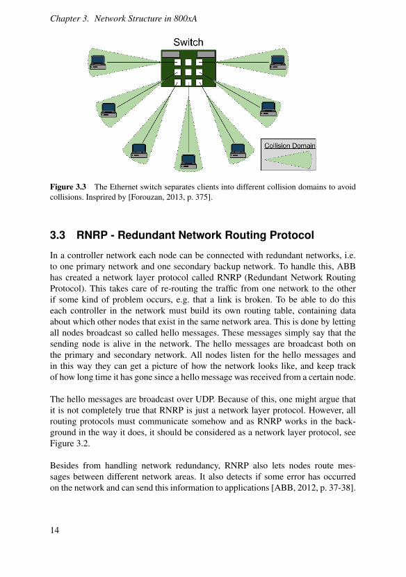
Switched Ethernet is an upgraded version of the CSMA/CD, that avoids collisionson the network by dividing a network of N clients into N collision domains byusing a switch, see Figure 3.3. In this way, collisions due to interfering traffic be-tween clients are eliminiated, as long as the switch is able to multiplex the differentchannels [Forouzan, 2013, p. 363-375].
13
Chapter 3. Network Structure in 800xA
Figure 3.3 The Ethernet switch separates clients into different collision domains to avoidcollisions. Insprired by [Forouzan, 2013, p. 375].
3.3 RNRP - Redundant Network Routing Protocol
In a controller network each node can be connected with redundant networks, i.e.to one primary network and one secondary backup network. To handle this, ABBhas created a network layer protocol called RNRP (Redundant Network RoutingProtocol). This takes care of re-routing the traffic from one network to the otherif some kind of problem occurs, e.g. that a link is broken. To be able to do thiseach controller in the network must build its own routing table, containing dataabout which other nodes that exist in the same network area. This is done by lettingall nodes broadcast so called hello messages. These messages simply say that thesending node is alive in the network. The hello messages are broadcast both onthe primary and secondary network. All nodes listen for the hello messages andin this way they can get a picture of how the network looks like, and keep trackof how long time it has gone since a hello message was received from a certain node.
The hello messages are broadcast over UDP. Because of this, one might argue thatit is not completely true that RNRP is just a network layer protocol. However, allrouting protocols must communicate somehow and as RNRP works in the back-ground in the way it does, it should be considered as a network layer protocol, seeFigure 3.2.
Besides from handling network redundancy, RNRP also lets nodes route mes-sages between different network areas. It also detects if some error has occurredon the network and can send this information to applications [ABB, 2012, p. 37-38].
14

3.3 RNRP - Redundant Network Routing Protocol
Figure 3.4 RNRP network topology, inspired by [ABB, 2012, p. 40].
If a network error occurs between two nodes in a network area, RNRP can only savethe connection if at least one of the networks, primary or secondary, is working forboth nodes. In Figure 3.4 five nodes exist in a network area. In this example, it doesnot matter if the nodes are controllers or workstations, as long as they are networknodes and use RNRP. As seen in Figure 3.4 node A and C have lost their connec-tion to the primary network and node E has lost the connection to the secondarynetwork. In this case, node A and C can communicate with all nodes except E. Thesame thing applies to E, i.e. it can communicate with both B and D but not with Aand C. Node B and D have a fully redundant connection [ABB, 2012, p. 40].
In the case of a network error, RNRP separates between two kinds of errors: linkdown and node down. Node down is when a controller is not responding at all,e.g. if it crashes or loses power. This is detected by other controllers by noticingthat hello messages are not sent from that controller. As default, three missed hellomessages are interpreted as a node down event. Link down could for example be ifan Ethernet cable is physically removed or cut off. A link down can be sensed by anetwork node and in case of a link down, RNRP can instantly redirect traffic, thatis, without waiting for three (as default) lost hello messages.
There is a bit more to know about RNRP, but this is out of scope for this report. For
15

Chapter 3. Network Structure in 800xA
more information see [ABB, 2012].
3.4 UDP - User Datagram Protocol
UDP is a connectionless and simple transport protocol. It is, along with TCP, usedin the transport layer of the ABB 800xA network structure. UDP has no featuressuch as flow, error or congestion control, however, its header does include a check-sum as seen in Figure 3.5. The resending of the lost or corrupted packets is notperformed by UDP, but has to be taken care of by protocols at a higher level (suchas IAC). As a result, there are no acknowledgements sent and information might belost or arrive out of order, at least at the transport layer.
UDP is a useful alternative to TCP when it is not disastrous if some packets arriveout of order or do not reach the destination at all. Under these conditions, UDPis preferable since it does not require connection establishment and terminationpackets to be sent and thus giving a more efficient transfer. Another case whereUDP could be preferred over TCP is when the user wants to be able to configurethe resend time-outs. This is not possible in TCP, but since UDP does not resendpackets at all, the resend scheme can be determined by a higher level protocol.
Figure 3.5 UDP header format. Inspired by [Forouzan, 2013, p. 738].
3.5 TCP - Transmission Control Protocol
TCP is a connection-oriented transport protocol [Forouzan, 2013, p. 999]. It is,along with UDP, used in the transport layer of the ABB 800xA network struc-ture. TCP is a reliable protocol with features such as flow, error and congestioncontrol. It is responsible for process-to-process communication and multiplexing is
16

3.5 TCP - Transmission Control Protocol
achieved using port numbers. The data is sent in byte-oriented segments ("stream ofbytes") between the sending and receiving buffers. The TCP header segment formatis shown in Figure 3.6.
Figure 3.6 TCP header format. Inspired by [Forouzan, 2013, p. 748].
Connection Establishment and TerminationThe TCP connection allows for transmission of data in both directions, which meansthat the communication must be initialized (and terminated) by both the server andthe client. Figure 3.7 shows events 1-7 described below.
Connection Establishment using three-way-handshaking
1. The client performs an active open by sending the first segment with a SYNflag set, requesting a connection from client to server. This consumes onesequence number.
2. The server responds with a SYN+ACK segment, which both requests a con-nection from server to client as well as acknowledges the client’s SYN re-quest. This consumes one sequence number.
3. The client responds with an ACK segment, acknowledging the server’s SYNrequest. The connection is now open in both directions, and this segment doesnot consume a sequence number.
17

Chapter 3. Network Structure in 800xA
Figure 3.7 Connection establishment and termination for a common TCP scenario. In-spired by [Forouzan, 2013, p. 760].
Connection Termination using four-way-handshaking
4. The client performs an active close by sending a segment with a FIN flag set,
18
3.5 TCP - Transmission Control Protocol
requesting to terminate the connection from client to server.
5. The server responds with an ACK segment, acknowledging the client’s FINrequest. The connection is still open from server to client, and data transfer isstill possible in that direction.
6. The server sends a FIN segment, requesting to terminate the connection fromserver to client.
7. The client responds with an ACK segment, acknowledging the server’s FINrequest. In order to prevent delayed packets being accepted by a later connec-tion, the client enters a TIME-WAIT state for 2 Maximum Segment Lifetimes(MSL). After the 2MSL time out and the ACK is received by the server, theconnection is terminated in both directions.
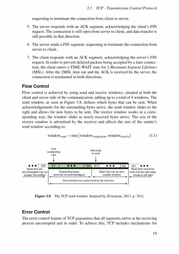
Flow ControlFlow control is achieved by using send and receive windows, situated at both theclient and server side of the communication, adding up to a total of 4 windows. Thesend window, as seen in Figure 3.8, defines which bytes that can be sent. Whenacknowledgements for the outstanding bytes arrive, the send window slides to theright and allows for new bytes to be sent. The receive window works in a corre-sponding way; the window slides as newly received bytes arrive. The size of thereceive window is advertised by the receiver and affects the size of the sender’ssend window according to:
windowsend = min(windowcongestion,windowreceive
)(3.1)
Figure 3.8 The TCP send window. Inspired by [Forouzan, 2013, p. 761].
Error ControlThe error control feature of TCP guarantees that all segments arrive at the receivingprocess uncorrupted and in order. To achieve this, TCP includes mechanisms for
19

Chapter 3. Network Structure in 800xA
detecting and resending corrupted and/or lost segments, and storing of out-of-ordersegments until the missing segments arrive. This is done by making use of check-sums, acknowledgements and time-outs.
The key component of the error control is the retransmission of segments. This isperformed when any of the two events occur:
• Retransmission Time Out (RTO)When the retransmission time out for the connection expires, TCP resendsthe bytes in the entire send buffer.
• Three Duplicate ACKsWhen three duplicate ACKs arrive, TCP resends the bytes in the entire sendbuffer. This feature is called fast retransmission, and helps to speed up theretransmission process.
To clarify the error control procedure, a simple example of how the TCP protocolhandles lost messages is given. Consider the following case, a network node, calledA, wants to send three bytes of data to another node B. To simplify the packetsequence numbers, each segment only carries the (unrealistic) value of one byte.This means that the three bytes of data will be sent in three different segments, withthe sequence numbers 1, 2 and 3. In a real case scenario, a packet typically carriesabout 1500 bytes, hence a segment will cover an interval of sequence numbers.With this being said, the following list of events in combination with Figure 3.9 willexplain the error control feature of TCP.
1. The three segments are sent from A. Segment 1 and 2 get lost on the way.
2. Segment 3 arrives out of order at B and is stored in a temporary receive buffer.B sends ACK 1 to indicate that A should resend from segment 1.
3. A retransmission time out occurs, and the three segments are resent. Since Adoes not know that segment 3 has arrived at B, segment 3 is also sent again.This time, segment 2 is lost.
4. B receives segment 1 and 3. Since segment 1 is in order, it can be deliveredto the application layer. ACK 2 is sent to indicate that A should resend fromsegment 2.
5. Two ACK 2 arrive at B. Notice that this means that the duplicate ACKscounter is set to one. A new retransmission time out occurs, and since Aknows that segment 1 has arrived, only segment 2 and 3 are resent. Segment3 gets lost on the way.
6. Segment 2 arrives, hence both segment 2 and 3 are in order and can be de-livered to the application layer. Notice that segment 3 did not arrive but was
20

3.5 TCP - Transmission Control Protocol
stored previously. ACK 4 is sent to indicate that A should send from segment4.
7. Only three segments should be sent, hence A is finished sending.
Figure 3.9 An example of how TCP error control handles lost packages.
21

Chapter 3. Network Structure in 800xA
Congestion ControlCongestion control is achieved in TCP by making use of a congestion window atsender site, cwnd, which when necessary limits the send window. The most com-mon TCP implementation today, Reno TCP, uses a congestion control scheme asseen in Figure 3.10.
The TCP connection begins in the slow start (SS) phase with cwnd =1 MSS (Maximum Segment Size). In this example the slow start threshold(ssthresh) is set to 16 MSS. When an ACK arrives in the SS phase, cwnd getsmultiplied by 2 which leads to an exponential increase. As seen in the figure att = 3 RTTs (Round Trip Times), this increase is interrupted when a time-out oc-curs, resetting ssthresh to cwnd/2 and then setting cwnd to 1. The SS phase thenstarts again before reaching ssthresh at t = 5 RTTs.
This causes TCP to reach the congestion avoidance (CA) state. In this state cwnd isupdated according to cwnd = cwnd+1 when an ACK arrives, leading to an additiveincrease. This goes on until either a time-out occurs or three duplicate ACKs arrive.The former case is not shown in the figure, however that would force the connectionback to the SS phase again.
At t = 13 RTTs three duplicate ACKs arrive, which causes the connection to enterthe fast recovery (FR) state. Here the ssthresh value is set according to ssthresh =cwnd/2, before updating cwnd to ssthresh+3. In the FR state, the increase of cwndbehaves as in SS until a new non-duplicate ACK arrives. This occurs at t = 15 RTTs,and causes the connection to re-enter the CA state, but this time with cwnd set tothe current value of ssthresh. In this example, the connection stays in the CA stateuntil the figure ends at t = 20 RTTs. However, it is obviously still possible for theTCP connection to switch between the SS, CA and FR states when the events asdescribed above occur.
22

3.6 IAC - Inter Application Communication
Figure 3.10 An overview of the phases of Reno TCP congestion control. Inspired by[Forouzan, 2013, p. 785].
3.6 IAC - Inter Application Communication
IAC is an application layer protocol, used for reading and writing variables betweencontrollers in the 800xA network. This is done over UDP, as opposed to the MMSprotocol which utilizes TCP. This makes IAC an alternative that is simpler to usethan MMS, since no connection has to be established before the variable exchangecan begin. In order to initialize a variable communication over IAC, it is only nec-essary to declare the direction of the variables in each controller; in (i.e. read), out(i.e. write) or in/out (i.e. read/write).
The communication models for the client and server side can be seen in Figure 3.11and Figure 3.12 respectively. The model is based on three main parts: the com-munication protocol, a protocol handler thread and a scheduler thread. The com-munication protocol defines the format of the sent messages, and allows for mul-tiple variables to be sent in each message. The protocol handler is responsible forthe communication between the client and the server, and implements the func-tions necessary for creating and receiving IAC messages. The scheduler thread runs
23

Chapter 3. Network Structure in 800xA
asynchronously to the protocol handler thread and is responsible for storing andfetching the variable values. This is done by performing cyclic copy-ins to 1131(short for IEC-61131) variable memory on the client side and copy-outs from thevariable memory on the server side. When the server receives a request for a vari-able value, the protocol handler thread performs a look-up to fetch the latest storedvalue (copy-out) [ABB, 2013a, p. 24-26].
Figure 3.11 The interaction of the client and the IAC protocol handler. Inspired by [ABB,2013a, p. 26].
Req
Res
Req
Res
Req
Res
Req
Res
Req
Res
1131 exec 1131 exec 1131 exec
Task Cycle Time
Copy-out
Scheduler
Protocol Handler
Communication Protocol
Copy-out Copy-outLook-up Look-up Look-up Look-up Look-up
Figure 3.12 The interaction of the server and the IAC protocol handler. Inspired by [ABB,2013a, p. 26].
Since UDP has no resending mechanism, IAC itself has to be responsible for theerror control. A request is resent by IAC if no response is received within the time-out interval, normally set to the period of which the IAC requests are sent. Theresend time out is, however, never by default set to a higher value than 500 ms. IACdoes indeed guarantee that a request is met by a response, but not that they arrive inorder [ABB, 2010, p.49-56].
24

3.7 MMS - Manufacturing Message Specification
3.7 MMS - Manufacturing Message Specification
The MMS protocol is built upon TCP and is used for exchanging variable data. It isimplemented in the application layer of the OSI model (see Figure 3.2).
Before doing any variable value exchanges, the MMS protocol has to create a con-nection, both in the TCP connection that it is built upon and at the MMS layer.When getting a variable value over MMS a client first has to send a request to aserver which holds the variable to be read. Then the server sends back the value ofthe variable, see Figure 3.13. In general, an MMS server can periodically send datawithout requests but this is not used in the 800xA system. Thus, a server can onlysend data if it has received a request for it first. Note that in this context, both clientand server refer to a role that an AC 800M controller takes. That is, a controllercan be both a client and a server depending on if it sends or receives a request. Theserver in this case should not be confused with e.g. a connectivity server [ABB,2010, p. 31-48, 165].
Figure 3.13 Exchange of variable value with MMS [Sisco, 1995, p. 10].
The MMS layer also limits the number of request on a TCP connection to three.
25

4Simulation of Real TimeNetwork DistributedSystems
In this master’s thesis, the main tool used is TrueTime, a Matlab/Simulink basedsimulator for real-time and networked systems [Cervin et al., 2003]. TrueTime hasbeen developed at the Department of Automatic Control at Lund University andsupports co-simulation of controller task execution in real-time kernels, networktransmissions, and continuous plant dynamics.
4.1 Simulation Tool Alternatives
As mentioned, TrueTime has been chosen as a tool for the simulation in this thesisproject, but there are several alternatives available. Below, a list of different networksimulators is presented. Also, some of the most commonly used network simulatorsare described in corresponding subsections later in this chapter [Pan, 2008]. Noticethat these are network simulators, not emulators. The difference is that a simulatorcatches the overall behaviour while an emulator mimics the reality "exactly". Sincewe are interested in looking at the overall behaviour, a simulator is preferred.
• NetSim - [tetcos, 2014], [Waupotitsch et al., 2006, p. 2135]
• ns-1 - [Floyd, 1999], [ns-3 Project Goals 2006]
• ns-2 - [Information Science Institution, 2011], [ns-3 Project Goals 2006]
• ns-3 - [ns-3 Homepage 2014], [The ns-3 Manual 2014], [ns-3 Project Goals2006]
• OPNET - [Riverbed Homepage]
26

4.1 Simulation Tool Alternatives
• OMNET++ - [Omnet++ Homepage]
• REAL - [REAL Homepage]
• SSFNet - [SSFNet Homepage]
• J-Sim - [J-Sim Homepage]
• QualNet - [QualNet Homepage]
Most network simulators are based on something called discrete event simulation(DES). This basically means that a number of events, and how the system reactsto these, are defined. In this way, very complex system can be modeled. Besidesfrom network simulations, discrete event simulation is often used in stress testing,finance, manufacturing and health care [Rouse, 2012]. Another method to simulatenetworks is by a Markov chain simulation. This is usually faster, but less detailedand flexible than discrete event simulation [Gkantsidis et al., 2003].
ns-2The ns-2 network simulator was made in collaboration between UC Berkeley, LBL,USC/ISI, and Xerox PARC, called the VINT project. It is an open source tool andit is supported by DARPA. The simulator is written in C++ and it uses OTcl forcommands and configuration. ns-2 is a newer version of ns-1 which is based on theREAL network simulator [Information Science Institution, 2011, p. 1].
ns-3The ns-3 network simulator is open source software and is widely used in research.It is programmed in C++ and was developed as a replacement for ns-2. Simulationsmade with ns-3 can be written in C++ and/or Python code. For more information,see [ns-3 Homepage 2014], [The ns-3 Manual 2014] and [ns-3 Project Goals 2006].
OPNETOPNET is a commercial network simulator made by Riverbed. It is, according toRiverbed’s own website, the fastest discrete event based network simulator on themarket. It has an open interface so that integration with other tools and simulatorsis easy. It has support for several protocols and devices and has rich visualization ofsimulation results. The tool is made in C/C++ [Riverbed Homepage].
OMNET++OMNET++ is actually not just a network simulator, but a discrete event simulatorin general. However, it is commonly used as just a network simulator. It consistsof components in C++ but it is used with a high level language called NED. Italso has some GUI support and an IDE based on the Eclipse platform [Omnet++Homepage].
27

Chapter 4. Simulation of Real Time Network Distributed Systems
Why TrueTime Was ChosenEven though there are many other good alternative tools for the simulation andTrueTime has some drawbacks, we consider TrueTime to best fit this project. Thisis especially thanks to the integration of TrueTime with Simulink which makes itvery easy to simulate physical processes in combination with the network and con-trol system. TrueTime can also be used to model the behaviour of the AC 800Mcontroller with the right amount of details. TrueTime lacks built in support for sim-ulation of protocols above the link layer, however, it has been reasonably "easy" toimplement this. Another desirable feature is that TrueTime is open source software,thus, access to the entire source code is provided.
4.2 TrueTime
TrueTime is a simulation tool based on Matlab/Simulink. It is developed at theDepartment of Automatic Control at LTH in Lund and is made for simulating real-time control systems.
Structure of a Simulation in TrueTimeA simulation with TrueTime is constructed with Simulink blocks from the TrueTimelibrary, see Figure 4.1. Right now, the available blocks are:
• TrueTime Kernel
• TrueTime Network
• ttGetMsg
• ttSendMsg
• TrueTime Battery
• TrueTime Wireless Network
• TrueTime Ultrasound Network
In this master’s thesis the only blocks used are the kernel and network blocks. Thekernel block represents a computing node that runs some user defined code, seeSection 4.2, and the network block corresponds to the physical and data link layer ofa (wired) network. TrueTime also gives the user the possibility to run the simulationwith either just Simulink blocks, or in a combination with code written in C++ orMATLAB m-files. These blocks and files can then be used together with standardSimulink blocks, e.g. a transfer function block representing a physical process. Thenthe TrueTime kernel and network blocks can act as a distributed control system thatcontrols the physical process [Cervin et al., 2010, p. 9].
28

4.2 TrueTime
Figure 4.1 The TrueTime block library
The Network BlockIn the TrueTime network block, a local area network is modelled. The block rep-resents the physical and data link layer of the OSI-model (see Figure 3.2). In theblock settings it is required to specify:
• Network Type
• Network Number
• Number of Nodes
• Data Rate
• Minimum Frame Size
• Loss Probability
29

Chapter 4. Simulation of Real Time Network Distributed Systems
• Initial Seed
• Other Network Type Specific Parameters
The network type sets what kind of data link layer protocol to be used. The currentnetwork types supported are:
• CSMA/CD (Ethernet)
• CSMA/AMP (CAN)
• Round Robin
• FDMA
• TDMA
• Switched Ethernet
• FlexRay
• PROFINET
• NCM
The network number is just an ID for the network and the number of nodes is,as the name indicates, how many nodes (kernel blocks) that are connected to thenetwork. Data rate sets the transfer speed of the network in bits/s and minimumframe size is the least amount of bits one packet is allowed to have. Loss probabilityis the probability of losing a packet when sending something over the network.This parameter and the data rate are what model the physical layer of the network.There is no possibility to specify a certain physical media, but it is not important tosimulate such details in this project anyway.
The Network block also outputs a network schedule. The schedule shows whichnetwork nodes that are currently active. An example of a network schedule is seenin Figure 4.2.
30

4.2 TrueTime
0 10 20 30 40 501
1.2
1.4
1.6
1.8
2
2.2
2.4
2.6
2.8
3
Time / s
Node s
tate
Network Schedule
Figure 4.2 A schedule over a simulated network in TrueTime. The different colours indi-cate different nodes in the network. When the schedule is at an integer value the node of thatnumber is idle. If the schedule shows a value of X + 0.5 where X is an integer, that node iscurrently using the network.
In addition to the network block there is a wireless network block. With this one can,as the name suggests, model a wireless network. There are a couple of parametersfor modeling typical attributes for a wireless network, such as path loss functionand signal strength. It also features the wireless network standards 802.11b WLANand 802.15.4 ZigBee [Cervin et al., 2010, p. 16-26].
The Kernel BlockIn TrueTime, the kernel block represents a real time kernel running some specifiedtasks (see Section 4.2 for information on tasks). What tasks the kernel should per-form is set in the so called init function, which is written in a MATLAB m-file orin C++. There are also a few parameters to set for each kernel block:
• init Function (as mentioned above)
• init Function Argument
31

Chapter 4. Simulation of Real Time Network Distributed Systems
• Number of Analog Inputs and Outputs
• Number of External Triggers
• (Network and) Node Numbers(s)
• Local Clock Offset and Drift
With the init function argument it is possible to send data to the init function.The number of analog inputs and output sets the amount of channels used to inter-act with other Simulink blocks. External triggers can be used for programming inSimulink rather than in the init functions. The network and node numbers tellsTrueTime what network(s) that kernel belongs to and what number (basically anIP) the kernel has in that network. When using multiple networks for one kernelthis should be an n×2 matrix where n is the number of networks connected to thekernel. Each row then contains a network number and a node number. Local clockoffset and drift sets the behavior of the clock used in the kernel.
The kernel block can output, in addition to the analog output(s), a schedule of therunning tasks and the kernels power consumption [Cervin et al., 2010, p. 15].
User Defined CodeAs mentioned earlier, TrueTime provides the possibility to control what each kernelblock should run in the simulation by specifying a user defined code written ineither a MATLAB m-file or in C++. The latter alternative is compiled with theMatlab MEX interface linked to an external C/C++ compiler (e.g. gcc or VisualStudio C++).
In the user defined code, tasks can be set to a kernel. These tasks can be performedboth periodically and on events. In the case of event driven task, a task could e.g.be triggered by an incoming packet on a network. In the code it is also possible tospecify the priorities and scheduling of tasks.
TrueTime CoreThis section describes the internal underlying machinery of TrueTime, i.e. how thesimulations are executed in the kernels.
The RTSys Class The main TrueTime core class that handles the simulations ina kernel is called RTSys. When the S-function corresponding to a specific kernelis initialized, i.e. the so called init function, an instance of RTSys is created andstored in the UserData field of the kernel block between simulation steps. It con-tains, among others, the attributes seen in Figure 4.3. The RTsys instance handlesthe actions that are executed in runKernel(), which is the main method where thetasks are run.
32

4.2 TrueTime
Figure 4.3 An overview of the RTSys class. The class responsible for running the simula-tion of the TrueTime kernels.
Task Execution TrueTime kernel tasks are handled by the readyQ and timeQmember variables in the RTSys class. Both queues are sorted linked lists and con-tain the tasks, as well as the timers, sorted in release and expiry time priorities. ThereadyQ is used for the tasks and timers that are ready for execution and the purposeof the timeQ is to keep track of the tasks and timers that are to be released [Cervinet al., 2010, p. 36-41].
The tasks in TrueTime are divided into segments. When a task is run, the task codewill be called repeatedly with an increasing segment number, starting with segmentone. It is not until the function returns FINISHED, i.e. -1, that the task code stopsgetting called. Due to this behaviour, a task code function typically consists of aswitch statement:
33

Chapter 4. Simulation of Real Time Network Distributed Systems
1 double taskCodeFunction(int seg, void* data)2 {3 switch (seg) {4 case 1:5 // Do something in the first "round"6 return someExecTime;7 case 2:8 // Do something in the second "round"9 return someMoreExecTime;
10 default:11 return FINISHED;12 }13 }
The return value of the code function is of type double and represents the taskexecution time. Note that this is not the actual execution time required by Matlab toexecute the simulations, rather it is an estimation provided by the user to representthe actions taking place. The void pointer data is used for passing variables to thecode function. Since it is a void pointer, anything can be passed, including arraysand structs to pass multiple values.
A task is always provided with a function pointer, which points to some user definedcode that specifies the actions that task should take. A simple pseudo-code exampleof adding a function pointer to a task is shown below:
1 double codeFunctionToBeAttached(int seg, void* data)2 {3 mexPrintf("This task is running!");4 return execTime;5 }6
7 ttCreatePeriodicTask("task_name", startTime, period,8 codeFunctionToBeAttached);
SummaryTrueTime is a powerful tool for simulation of control system distributed over net-works. It provides the user a good base to create highly customizable simulations.However, due to its openness it requires a lot of knowledge from the user, both aboutthe system to be simulated and about TrueTime.
34

5Modeling and Simulation of800xA
This chapter describes the implementation of the 800xA network structure in True-Time, which mainly consists of adding the features of higher level protocols suchas TCP and RNRP. In addition to the network protocols, the main threads in thecontrollers are also considered in order to model the behaviour of the controllers asaccurate as possible.
5.1 Helper File
In order to make it easier to create different simulation setups, a helper file has beencreated to encapsulate the behaviour of general 800xA components. For example,the behaviour of how to handle a TCP connection is put in the helper file, while theinit script of a kernel contains the connections it needs to use. In other words, eachkernel defines its behaviour in the init script, but uses the predefined utilities of thehelper file. The helper file could thus be viewed as an extension to TrueTime withthe features of higher level protocols and the AC 800M controller.
Worth mentioning is that the helper file has been made so that not too much flexi-bility is lost. It is still easy to e.g. write custom PID code for a single kernel.
The helper file has a rather complicated class structure. This can be seen in Figure5.1. Notice that this is just an overview, more detailed diagrams and explanationsare found in corresponding sections.
5.2 Implementation in TrueTime
TrueTime has built in support for simulation of the physical and data link layersin networks. For simulation of communication with higher layer protocols such as
35

Chapter 5. Modeling and Simulation of 800xA
Figure 5.1 A class overview of the protocol_helper.cpp file.
TCP and MMS, a file protocol_helper.cpp has been implemented. To simulatethe internal behaviour of the controllers, tasks are utilized to model the most impor-tant threads.
Kernel Setup and initVital() FunctionWhen using the helper file some parts of the kernel setup are vital for the otherfunctions to work properly. Some of these essential commands, the ones that everykernel must run, have been collected in a function called initVital(). This func-tion is responsible for defining events, starting tasks and network handlers for dualnetworks. A full list of its responsibilities is shown below:
• Creating Internal Mailboxes:
– tNet0ActionType
– tNet0
– tNet0Down
– iacSendDownSignalMail
36
5.2 Implementation in TrueTime
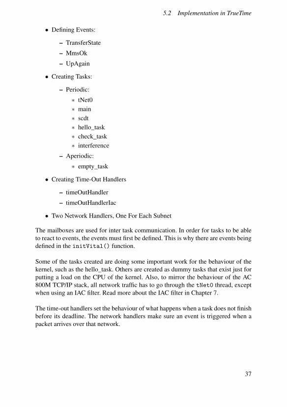
• Defining Events:
– TransferState
– MmsOk
– UpAgain
• Creating Tasks:
– Periodic:
∗ tNet0∗ main∗ scdt∗ hello_task∗ check_task∗ interference
– Aperiodic:
∗ empty_task
• Creating Time-Out Handlers
– timeOutHandler
– timeOutHandlerIac
• Two Network Handlers, One For Each Subnet
The mailboxes are used for inter task communication. In order for tasks to be ableto react to events, the events must first be defined. This is why there are events beingdefined in the initVital() function.
Some of the tasks created are doing some important work for the behaviour of thekernel, such as the hello_task. Others are created as dummy tasks that exist just forputting a load on the CPU of the kernel. Also, to mirror the behaviour of the AC800M TCP/IP stack, all network traffic has to go through the tNet0 thread, exceptwhen using an IAC filter. Read more about the IAC filter in Chapter 7.
The time-out handlers set the behaviour of what happens when a task does not finishbefore its deadline. The network handlers make sure an event is triggered when apacket arrives over that network.
37

Chapter 5. Modeling and Simulation of 800xA
5.3 Simulating RNRP with TrueTime
In this section, the implementation of the routing protocol RNRP (see Section 3.3) inTrueTime is described. The following aspects of the protocol have been considered:
• Hello messages
• Creating routing tables
• Routing using table lookup
• Network failure redirection
The implementation of keep-alive hello messages is achieved simply by sendingbroadcast messages from each alive kernel, using the TrueTime predefined functionttSendMsg() (see [Cervin et al., 2010, p.95]). The messages are sent periodicallywith a default 1 s period by making use of a periodic task created by the predefinedfunction ttCreatePeriodicTask() (see [Cervin et al., 2010, p.65]). Since everykernel has to send these hello messages, this is part of the method initVital()(see Section 5.2). The messages consist of static pointers to instances of Hel-loPackets, a class that inherits from the base class Packet. The HelloPacket classis identical to Packet, apart from that it overrides the getType() method to signalthat it is part of a hello message. The member variables of the Packet class can beseen in Figure 5.2.
38

5.3 Simulating RNRP with TrueTime
Figure 5.2 Overview of the class structure used for sending packets inprotocol_helper.cpp
39
Chapter 5. Modeling and Simulation of 800xA
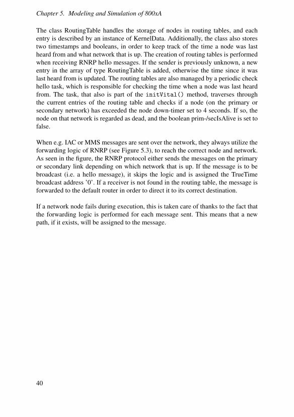
The class RoutingTable handles the storage of nodes in routing tables, and eachentry is described by an instance of KernelData. Additionally, the class also storestwo timestamps and booleans, in order to keep track of the time a node was lastheard from and what network that is up. The creation of routing tables is performedwhen receiving RNRP hello messages. If the sender is previously unknown, a newentry in the array of type RoutingTable is added, otherwise the time since it waslast heard from is updated. The routing tables are also managed by a periodic checkhello task, which is responsible for checking the time when a node was last heardfrom. The task, that also is part of the initVital() method, traverses throughthe current entries of the routing table and checks if a node (on the primary orsecondary network) has exceeded the node down-timer set to 4 seconds. If so, thenode on that network is regarded as dead, and the boolean prim-/secIsAlive is set tofalse.
When e.g. IAC or MMS messages are sent over the network, they always utilize theforwarding logic of RNRP (see Figure 5.3), to reach the correct node and network.As seen in the figure, the RNRP protocol either sends the messages on the primaryor secondary link depending on which network that is up. If the message is to bebroadcast (i.e. a hello message), it skips the logic and is assigned the TrueTimebroadcast address ’0’. If a receiver is not found in the routing table, the message isforwarded to the default router in order to direct it to its correct destination.
If a network node fails during execution, this is taken care of thanks to the fact thatthe forwarding logic is performed for each message sent. This means that a newpath, if it exists, will be assigned to the message.
40

5.3 Simulating RNRP with TrueTime
Figure 5.3 The forwarding logic of RNRP.
41

Chapter 5. Modeling and Simulation of 800xA
5.4 Simulating TCP with TrueTime
This section describes the way the TCP protocol has been implemented in theprotocol_helper.cpp helper file.
The TCP Connection ClassThe TCP connection class is responsible for handling the traffic between two kernelsover a certain TCP connection. An overview of the class can be seen at Figure 5.4.It contains information of:
• The IP of the host and destination
• The name of the host and destination
• The source port of the host and destination
• Sequence count (Next segment to send)
• Integer of the last ACK that has been sent
• Integer of the last segment that has been received
• A send window and a receive window
• A state of the connection (INIT, TRANSFER, CLOSE or REINIT)
• A counter of number of duplicate ACKs in a row
• Send-, receive- and a temporary (for unordered packets) buffer
• A list of all transmitted TCP packets (for later deletion)
• An MMS variable counter
42

5.4 Simulating TCP with TrueTime
Figure 5.4 An overview of the TcpConnection class, the class responsible for handling aTCP connection in the protocol_helper.cpp file.
43

Chapter 5. Modeling and Simulation of 800xA
Connection Establishment and TerminationBefore transmitting data over the TCP connection, a connection must be es-tablished from both client and server kernel. This has been implementedby a call to Kernel::openTcpConnection("OtherKernel", sourcePort,destinationPort), which initializes all required variables and adds the con-nection to the list of TCP connections in the kernel. This also initiates a three-way handshake as described in Section 3.5, and during the establishment processthe state of the connection is set to INIT where further data transfer is blocked.When the connection establishment is finished in both ways, the event Transfer-State is triggered and puts the connection to state TRANSFER allowing for datacommunication. In the same way, a connection can be terminated by a call toKernel::closeTcpConnection(TcpConnection* tcp). This issues a four-way handshake termination process, as well as freeing used memory and removingthe connection from the TCP connections list in the kernel.
Sending and Receiving DataThe sending and receiving mechanism has been made in layers. This is mainly forsimplifying the rather complex logic but it also follows the design a real TCP/IPstack is using. The job of the TCP connection is to go from Application layer, inthis case the MMS protocol, to the RNRP protocol at the network layer (see Fig-ure 3.2). To facilitate the implementation of the TCP/IP stack, the MMS protocolfunctionality was merged into the TcpConnection class, but this part is covered inSection 5.6.To send a packet over an established connection, one must first check the TCPstatus with a call to TcpConnection::send(). Then, to actually start the sendingprocess, a call to TcpConnection::put() is made. The application code in thesender can look something like this:
44
5.4 Simulating TCP with TrueTime
1 TcpConnection* tcp = kernel->getTcpConnection(port);2
3 switch (seg) {4 case 1:5 status = tcp->send(length, currentStateOfConnection)6 // Handle status..7 if(Has to wait) {8 // Go back to this code segment9 // in next method call
10 }11 if(Send buffer is full) return FINISHED;12 if(No problems) return 0.0;13 return someWaitingExecTime;14 case 2:15 tcp->put(msgData, length);16 return someExecTime;17 default:18 return FINISHED;19 }
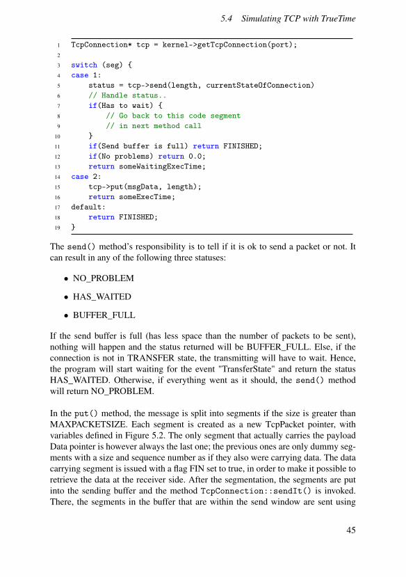
The send() method’s responsibility is to tell if it is ok to send a packet or not. Itcan result in any of the following three statuses:
• NO_PROBLEM
• HAS_WAITED
• BUFFER_FULL
If the send buffer is full (has less space than the number of packets to be sent),nothing will happen and the status returned will be BUFFER_FULL. Else, if theconnection is not in TRANSFER state, the transmitting will have to wait. Hence,the program will start waiting for the event "TransferState" and return the statusHAS_WAITED. Otherwise, if everything went as it should, the send() methodwill return NO_PROBLEM.
In the put() method, the message is split into segments if the size is greater thanMAXPACKETSIZE. Each segment is created as a new TcpPacket pointer, withvariables defined in Figure 5.2. The only segment that actually carries the payloadData pointer is however always the last one; the previous ones are only dummy seg-ments with a size and sequence number as if they also were carrying data. The datacarrying segment is issued with a flag FIN set to true, in order to make it possible toretrieve the data at the receiver side. After the segmentation, the segments are putinto the sending buffer and the method TcpConnection::sendIt() is invoked.There, the segments in the buffer that are within the send window are sent using
45

Chapter 5. Modeling and Simulation of 800xA
tNet0Send().
However if the to the put() method passed Data pointer is null, the packet istreated as an ACK and instead directly passed to the TcpConnection::sendAck()method. The ACK packets are thus not entered into the send buffer, rather they aresent independently as they are not included in the flow control. Read more aboutthis in Section 5.4.
On the receiver side, the code could roughly look like this:
1 TcpConnection* tcp = kernel->getTcpConnection(port);2
3 switch (seg) {4 case 1:5 tcpPackets = tcp->get();6 return someExecTime;7 default:8 return FINISHED;9 }
The only thing the get() method does, is to loop through the receive buffer until apacket with FIN flag set to 1 is found.
Flow ControlFlow Control is implemented in TrueTime using two instances of class Buffer (bothsend and receive) in each kernel. The send and receive windows are implemented assimple integers in the TcpConnection class. This means that they represent absolutesequence numbers rather than intervals, i.e. if the seqCount variable is smaller thansendWindow, it is regarded as within the allowed send window.
Error ControlThe TCP protocol must ensure that data arrives and is in correct order. As men-tioned in Section 3.5, the TCP protocol uses an ACK mechanism to ensure packetarrival and order. The ACK packets are created and sent in the sendAck() methodupon arrival of a new segment.
The resending due to time-outs is taken care of by the interrupt handler time-OutHandler and its code function timeOutCode(). As each sent packet is as-signed with a resend timer, by default set to 1 s, the expiration of such a timerwill trigger an interrupt and thus execute the time-out code. This function callsTcpConnection::resendAllInSendBuffer(), which utilizes the sendIt()method to resend the packets and reset all timers.
46

5.5 Simulating IAC with TrueTime
The other reason for a resend that is implemented is the arrival of three consecutiveduplicate ACKs. This is implemented by a duplAcks counter in the TcpConnectionclass, which is increased each time when the ACK arrived is equal to lastAck. Whenit reaches a value of three the method resendAllInSendBuffer() is invoked andthe counter is reset. The counter is also reset when a new ACK, e.g. greater thanlastAck, arrives.
To guarantee that the segments arrive in order at the application layer, they are storedin a temporary receive buffer tmpRcvBuffer that is part of the TcpConnection class.Upon arrival of each segment, the tmpRcvBuffer is sorted and all segments that arein order and greater than the lastRcv segment are emptied from the tmpRcvBufferinto the (final) rcvBuffer.
Congestion ControlThe implementation of congestion control in our version of TCP in TrueTime is leftout. This is due to the fact that congestion in the network is not very likely since themessages are typically sent with a ~1 second periodicity.
5.5 Simulating IAC with TrueTime
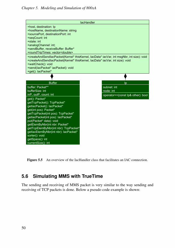
As mentioned in Section 3.6, the IAC protocol is connectionless and is based onUDP. The IAC protocol however, has its own resending mechanism. The IacHan-dler can be used in a similar fashion as the TcpConnection, and an overview of theclass can be seen in Figure 5.5. To set up an IAC handler simply write the followingin an init script of a kernel:
1 kernel->createIacHandler("OtherKernel", sourcePort,2 destinationPort, analogChannel);
Here the analogChannel specifies what channel to use when handling IAC mes-sages. To use the IAC handler, one must first set up the IAC handler in the twokernels that should communicate. This is done as described above. Then in sometask code, a packet must be created and sent from the sender and received at thereceiver. This is shown in the pseudo code below:
47

Chapter 5. Modeling and Simulation of 800xA
Sender
1 IacHandler* iac = kernel->getIacHandler(port);2
3 switch (seg) {4 case 1:5 iacReq = new IacVariable<MeasurementToControlSignal>(6 "variable_name", value, isRequest);7 return someExecTime;8 case 2:9 iac->waitCheck();
10 return 0.0;11 case 3:12 iac->createAndSendIacPacket(kernel, iacReq, size);13 return someExecTime;14 default:15 return FINISHED;16 }
First, the IAC handler must be obtained by extracting it from the kernel, given acertain port number. Then in a first code segment (for an explanation of the segmentstructure used in this code, see Section 4.2), an IacVariable is created with the nameand value of the variable to be exchanged. Also, a flag indicating that the packet is arequest is set to true. The waitCheck() method in the second segment is handlingthe possible waiting due to network failures. In the third and last segment, the packetis sent. The IacHandler::send() method checks for a setting IAC_FILTER, seeChapter 7. If the filter is activated, the send() method ignores the normal wayto send a packet, i.e. through the tNet0 task, and just sends the packet with theTrueTime predefined function ttSendMsg(). If the filter is not activated the normalcall to tNet0Send() is used.
48

5.5 Simulating IAC with TrueTime
Receiver
1 IacHandler* iac = kernel->getIacHandler(port);2 IacPacket* iacPacket;3 Data* tmp;4 IacVariable<MeasurementToControlSignal>* var;5
6 switch (seg) {7 case 1:8 iac->waitCheck();9 return 0.0;
10 case 2:11 iacPacket = iac->get();12 var = dynamic_cast<IacVariable<MeasurementToControlSignal>*>(13 iacPacket->data);14 tmp = iacPacket->data->handle(kernel, port);15 return someExecTime;16 default:17 return FINISHED;18 }
As in the case of the sending kernel, the receiving kernel must obtain the IacHandlerinstance with getIacHandler(port). In the first segment, a waitCheck is performedto handle possible network failures. In the next segment, the packet can be receivedand data can be extracted. This is done with the IacHandler::get() method thatsimply gets a packet from the IAC handlers receive buffer. In addition, the data canbe "handled", which means that the receiving kernel somehow uses the data and itcan also return a value used for a reply to the sending kernel. This reply can, forexample, be a control signal.
When an IAC packet is created, a timer with an attached time-out handler is addedto the packet. If the timer expires, i.e. a packet does not arrive in time, a special time-out handler code, called iacTimeOutCode(), is executed. This code is responsiblefor resending this individual packet (not a group of packets as in the TCP case).
49
Chapter 5. Modeling and Simulation of 800xA
Figure 5.5 An overview of the IacHandler class that facilitates an IAC connection.
5.6 Simulating MMS with TrueTime
The sending and receiving of MMS packet is very similar to the way sending andreceiving of TCP packets is done. Below a pseudo code example is shown:
50

5.6 Simulating MMS with TrueTime
Sender
1 TcpConnection* tcp = ctrl->getTcpConnection(port);2
3 switch (seg) {4 case 1:5 // TRANFER is the wanted state6 status = tcp->mmsSend(size, TRANSFER);7 // Handle status..8 if(Has to wait) { // The waiting now includes TOO\_MANY\_MMS wait9 // Go back to this code segment
10 // in next method call11 }12 if(Send buffer is full) return FINISHED;13 if(No problems) return 0.0;14 return someWaitingExecTime;15 case 2:16 tcp->mmsPut(mmsReq, port);17 return someExecTime;18 default:19 return FINISHED;20 }
Here, the TcpConnection::mmsSend() and TcpConnection::mmsPut() basi-cally calls the TcpConnection::send() and TcpConnection::put() but withthe added functionality that the MMS connection only allows three outstandingMMS packets. Thus, for example, the TcpConnection::mmsSend() added a sta-tus TOO_MANY_MMS to indicate that the sender must wait for a currently out-standing MMS packet to be received before trying to send another one.
Receiver
1 TcpConnection* tcp = kernel->getTcpConnection(port);2
3 switch (seg) {4 case 1:5 tcpPackets = tcp->mmsGet();6 return someExecTime;7 default:8 return FINISHED;9 }
The TcpConnection::mmsGet() does, unlike TcpConnection::mmsSend() andTcpConnection::mmsPut(), use the TCP version of the method. This is becausethe use of TcpConnection::get() will extract any packet from the receive buffer.
51

Chapter 5. Modeling and Simulation of 800xA
In the MMS case, only the MMS packets should be extracted.
52

6Results of TrueTimeSimulations
This chapter covers the utilization of the implemented simulation. An example setuphas been made for model experimenting, see Section 6.1. The chapter also includesanalysis of the obtained simulation data and how to interpret some measures ofperformance.
6.1 Sensor/Actuator - Regulator Example
An example simulation has been made containing two controllers communicatingover a redundant network with MMS and IAC. This has been chosen to keep thingsas simple as possible, but so that it still produces some interesting results.
One of the controllers takes the role as a sensor/actuator node and the other actsas a regulator node. The sensor/actuator works as a client that periodically takesa measurement from a "physical" process. Then it sends the measurement to theregulator as a request for a control signal. The regulator computes the control signaland sends it back to the sensor/actuator which sets the control signal to the process.To make it easier to compare the performance of IAC and MMS, the example hastwo identical processes, one controlled by sending IAC packets and one with MMSpackets.The simulation can be run with disturbances of the following kind:
• Measurement noise
• Packet loss probability
• Network interference load
• Interfering kernel tasks
53

Chapter 6. Results of TrueTime Simulations
Figure 6.1 The regulator example Simulink blocks.
The process has been chosen to have a proper time constant so that interestingresults are obtained from a simulation. The typical ABB customer system is somekind of process industry. In such a system it is usually more important to stayclose to a certain reference during load disturbances rather than quickly respond toreference changes. This has been taken into consideration in the simulations and aprocess with a square wave as load disturbance is used.
The regulator node uses a discretized PID control algorithm with tracking basedanti wind-up, implemented in the code below:
54

6.1 Sensor/Actuator - Regulator Example
1 double calcFunction(PidData* pid, double y, double r)2 {3 double P = pid->K*(pid->beta*r-y);4 double I = pid->Iold;5 double D = pid->ad*pid->Dold + pid->bd*(pid->yold-y);6 double u = P + I + D;7
8 double uMax = 10;9 double uMin = -10;
10 double uNonSat = u;11
12 if (u > uMax) u = uMax;13 if ( u < uMin) u = uMin;14
15 pid->Dold = D;16 pid->Iold = (pid->Ti > 0) ? I +17 (pid->K*pid->h/pid->Ti)*(r-y) +18 (pid->h/pid->Tr)*(u - uNonSat) : 0;19 pid->yold = y;20
21 return u;22 }
First, the P, I and D parts of the control signal are calculated. Then, the signal issaturated, and finally, the "old" values of the PID parts are stored. However, noticethat the I part uses a tracking-based algorithm for anti wind-up. The observantreader notices the use of the PidData class. The PidData class contains informationof the PID settings used. It can also be used to "store" a function describing a con-trol signal algorithm as the one above. An excerpt from the PidData class is shownbelow:
55

Chapter 6. Results of TrueTime Simulations
1 class PidData : public Data {2 public:3 // ctrl params4 double K, Ti, Td, N, h, ad, bd, beta, Tr;5
6 // ctrl states7 double yold, Iold, Dold, u;8
9 double (*calcFunction)(PidData* pid, double y, double r);10
11 PidData(string name, double k, double ti, double td,12 double tr, double beta, double n, double h,13 double (*calcFcn)(PidData* pid, double y, double r))14 : K(k), Ti(ti), Td(td), Tr(tr), beta(beta), N(n), h(h),15 yold(0.0), Dold(0.0), Iold(0.0), u(0.0), calcFunction(calcFcn)16 {17 variableName = name;18 ad = Td/(N*h+Td);19 bd = N*K*ad;20 }21 // Some other stuff here22 };
In the simulations made in this master’s thesis, the following PID settings found inTable 6.1 have been used. These have been manually tuned for reasonable perfor-mance of the system.
Parameter ValueK 0.85Ti 3.5Td 0.5Tr
Ti+Td2
N 100β 1h 1
Table 6.1 The PID settings used in the simulations.
6.2 Measuring Performance
To get some kind of result from a simulation, a way of measuring performance isneeded. Hence, it is logical to separate between network, kernel and control perfor-
56

6.2 Measuring Performance
mance. The control performance is directly dependent on the other two but it is stillgood to be able to analyze them separately.
Network PerformanceTo measure the network performance, two aspects have been studied: network uti-lization and round trip times (RTT). The network utilization is calculated using thenetwork schedule from the network block in Simulink. The calculation is done by aMATLAB script that first defines a plot interval and makes a time weighted averagefor the scheduling values in each interval. Notice that due to the nature of discreteevent simulation there will be a lot of values in some time intervals and fewer inother. This is why the time weighted average is done. After this a smoothing filteris used on the averaged values.
This might seem a bit unscientific and it is too. There is no good definition of utiliza-tion and when you think about it, utilization in reality can only be 1 (something ishappening) or 0 (nothing is happening). This smoothing is just making it easier fora human to interpret the result. Below the code for calculating "smooth" utilizationis shown.
57

Chapter 6. Results of TrueTime Simulations
1 function [ smooth_util plot_t ] = calc_util( schedule, plot_interval )2 %CALC_UTIL Calculates a smooth util from schedule3 t = schedule.time;4 util = zeros(max(t)/plot_interval, 1);5 momentan_util = schedule.signals.values;6 util_size = size(momentan_util);7 util_rows = util_size(1);8 util_cols = util_size(2);9 d = diag(1:util_cols);
10
11 %norm to interval 0 - 0.512 momentan_util = momentan_util - (ones(util_size)*d);13
14 %for total requested util15 momentan_util = momentan_util > 0.13;16 total_momentan_util = zeros(length(momentan_util), 1);17
18 for j = 1:util_cols19 total_momentan_util = total_momentan_util + momentan_util(:,j);20 end21
22 i = 1;23 val = total_momentan_util(1);24 while(i <= util_rows)25 i_old = i;26 i = find(total_momentan_util(i:end) ~= val, 1) + i - 1;27 if(isempty(i))28 break;29 end30 util(ceil(t(i)/plot_interval)) = val*(t(i) - t(i_old));31 val = total_momentan_util(i);32 end33
34 util = util./plot_interval;35 smooth_util = smooth(util, 50, ’lowess’);36 plot_t = plot_interval:plot_interval:max(t);37 end
The smooth command with the ’lowess’ parameter is using a local regres-sion with weighted linear least square to smooth the data. See http://www.mathworks.se/help/curvefit/smooth.html for more information about thesmooth command. In Figure 6.2 a smoothed network utilization plot is shown. Com-pare this to Figure 4.2 which is the schedule used for the smooth plot.
58

6.2 Measuring Performance
0 10 20 30 40 500.03
0.035
0.04
0.045
0.05
0.055
Network 1 Bandwidth Utilization
Time (s)
Bandw
idth
Utilization
Figure 6.2 A smooth plot of the network utilization.
The round trip times are calculated by comparing the time of when a request issent from a client at application layer, to the time when the reply of this request isreceived at the application layer.
Kernel PerformanceThe same code described in the network performance section above can be used tocalculate CPU utilization from the schedule given by the kernel blocks.
Control PerformanceThere are several ways to measure the control performance of a system and some ofthe most common ones are overshoot, settling time and rise time of a step response.However, in process industry, which is where the 800xA system is mostly used, oneis often interested to stay as close to a static reference as possible rather than fol-lowing a reference change. Due to this, it is more interesting to look at performancemeasures that somehow integrate the error term over time. Below are the chosenmeasures in order to evaluate control performance:
• IAE - Integral Absolute Error
59

Chapter 6. Results of TrueTime Simulations
• ISE - Integral Squared Error
• ITAE - Integral Time Absolute Error
IAE =∫ T
0|e(t)|dt (6.1a)
ISE =∫ T
0(e(t))2 dt (6.1b)
ITAE =∫ T
0t|e(t)|dt (6.1c)
IAE is simply integrating the distance from the reference. ISE has the property thatlarge deviations from the reference will have a much larger impact on the ISE valuethan smaller deviations. In ITAE the time t is started at some kind of step, either inreference or in a load disturbance. The weighting with t makes ITEA sensitive toovershoot and oscillations.
6.3 Handling of Packet Losses
In a real network, packets do not always get to their destinations. This is referred toas a packet loss. In TrueTime, each network can set the loss probability, that is, theprobability of losing a packet when sending it. As the MMS and IAC protocols usedifferent ways of handling lost packets, it is interesting to measure and compare theperformance of systems using MMS and IAC to communicate.
Simulations have been run with four different loss probabilities: 0 %, 0.1 %, 1 %and 10 %. For each setup, plots of the measurement signal and control signal havebeen studied as well as the performance measures described in Section 6.2.
Below in Table 6.2, the performance measures from the simulations are presented.In general, the IAC protocol is better than the MMS protocol for handling frequentpacket losses. But with low loss probabilities, the difference is very small. In a realnetwork, the loss probability is often very small. For instance, in the measurementsdone on a real system in this master’s thesis, no packet losses were recorded.
At 10 % loss probability, the IAC protocol is a clear winner as the MMS protocolhas 16.26 % higher IAE, 27.84 % higher ISE and 19.79 % higher ITAE. This is,however, an extreme case with very high loss probability. Though, it should benoticed that the process to be controlled could be of a more difficult nature. That is,the 10 % loss probability might be extreme, but the process in a real system could
60
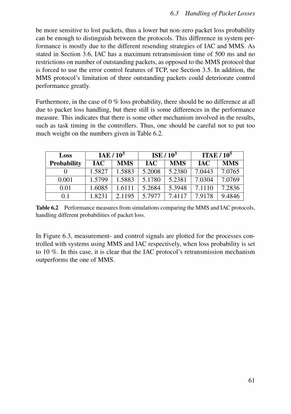
6.3 Handling of Packet Losses
be more sensitive to lost packets, thus a lower but non-zero packet loss probabilitycan be enough to distinguish between the protocols. This difference in system per-formance is mostly due to the different resending strategies of IAC and MMS. Asstated in Section 3.6, IAC has a maximum retransmission time of 500 ms and norestrictions on number of outstanding packets, as opposed to the MMS protocol thatis forced to use the error control features of TCP, see Section 3.5. In addition, theMMS protocol’s limitation of three outstanding packets could deteriorate controlperformance greatly.
Furthermore, in the case of 0 % loss probability, there should be no difference at alldue to packet loss handling, but there still is some differences in the performancemeasure. This indicates that there is some other mechanism involved in the results,such as task timing in the controllers. Thus, one should be careful not to put toomuch weight on the numbers given in Table 6.2.
LossProbability
IAE / 103 ISE / 103 ITAE / 105
IAC MMS IAC MMS IAC MMS0 1.5827 1.5883 5.2008 5.2380 7.0443 7.0765
0.001 1.5799 1.5883 5.1780 5.2381 7.0304 7.07690.01 1.6085 1.6111 5.2684 5.3948 7.1110 7.28360.1 1.8231 2.1195 5.7977 7.4117 7.9178 9.4846
Table 6.2 Performance measures from simulations comparing the MMS and IAC protocols,handling different probabilities of packet loss.
In Figure 6.3, measurement- and control signals are plotted for the processes con-trolled with systems using MMS and IAC respectively, when loss probability is setto 10 %. In this case, it is clear that the IAC protocol’s retransmission mechanismoutperforms the one of MMS.
61

Chapter 6. Results of TrueTime Simulations
0 50 100 150 200 250 300 350
−2
0
2
4
Reference and Measurement Signals
Ref/Load
MMS
IAC
0 50 100 150 200 250 300 350−4
−2
0
2
4Load Disturbance and Control Signals
Time / s
Figure 6.3 When the packet loss probability is set to 10 % the system performs poorly, butthe IAC protocol handles the lost packets better than the MMS protocol.
6.4 Investigating RNRP Settings
As mentioned, the 800xA system has the possibility to use redundant networks.This is handled by the RNRP protocol and as complex as the system is, it is hardto tune the RNRP settings. Hence, a possibility to quickly test different setups withhelp from a simulation is desirable. In this section a closer look is taken at some ofthe attributes of RNRP.
Network FailureA possible situation in a system is that a controller’s network stops working. InFigure 6.4 and Figure 6.5, a simulation example of when this happens is provided.In a simple system like this there is not much to analyze, but in larger systemswith many nodes, investigating what happens when a link down event occurs canbe more interesting. At least, this simple simulation shows that the MMS and IACprotocols handle a link down event differently. The IAC protocol takes action more
62

6.4 Investigating RNRP Settings
quickly, which leads to a faster but a bit more oscillating recovery.
0 50 100 150 200−4
−2
0
2
4Reference and Measurement Signals
Ref/Load
MMS
IAC
0 50 100 150 200−4
−2
0
2
4Load Disturbance and Control Signals
Time / s
Figure 6.4 Control and measurement signals when the Sensor/Actuator nodes primary net-work is destroyed at t = 50 s. RNRP redirects network traffic for the Sensor/Actuator con-troller to network 2. Also, notice the slightly different handling of the recovery from switch-ing by the MMS and IAC protocols.
Figure 6.5 clearly shows that all traffic is stopped for the Sensor/Actuator node(Node 1 in the plot) in Network 1, while the traffic is increased in Network 2. Aplot of the total network utilizations is left out as the total load on the network is notinteresting in this case. Also, the change in network load is rather small, as Network1 still is loaded with traffic of hello packets from the Regulator node.
63

Chapter 6. Results of TrueTime Simulations
0 50 100 150 2001
1.5
2
2.5
3
Network 1 Traffic
Time / s
Node S
tate
0 50 100 150 2001
1.5
2
2.5
3
Network 2 Traffic
Time / s
Node S
tate
Figure 6.5 The schedules for Network 1 and Network 2 respectively when the Sen-sor/Actuator nodes primary network is destroyed at t = 50 s. RNRP redirects network trafficfor the Sensor/Actuator controller to network 2 which is illustrated by the lack of traffic fornode 1 (The Sensor/Actuator controller) in Network 1 and the increased traffic in Network 2for the same node.
Lost Hello Packets AllowedIn Section 3.3 it is described how the RNRP protocol handles lost hello packets.As default, three hello packets must be lost before RNRP switches to the backupnetwork. Though, this number has been decided in an ad hoc manner and it wouldbe nice to be able to experiment with different numbers of allowed last hello packets.
It is preferable to keep robustness against occasionally dropped packets, but on theother hand, a fast detection of a broken node is also desirable. The first would re-quire a high number and the latter a low, i.e. it is a matter of opinion of what is mostimportant. A typical argument would be that it is more important to keep robustnessagainst false alarms rather than a fast recovery from a node down event as this issomething that should not happen very often. Also, switching between networkstakes one hello packet period to do, which definitely should be avoided. This is ofcourse very subjective and the importance of each aspect is highly dependent on
64

6.4 Investigating RNRP Settings
what system that is to be controlled. Anyway, a simulation could ease the decision.
In order to trigger node down events often enough to see something interestingin the simulations, the packet loss probability has been set to 10 % which is a lotconsidering how good modern networks are. Then, the number of lost hello packetsallowed has been changed from 0 to 3. At 3 allowed lost hello packets, no nodedown events were triggered, making it meaningless to run simulations with morethan 3 allowed lost hello packets. With this in mind one can come to the conclusionthat 3 allowed lost hello packets is a very robust setting, making false alarms ofnode down events almost impossible, even on bad networks.
Figure 6.6 shows simulation data from a setup using 0 lost hello packets allowed.This introduces a lot of network switching, but it occurs in such a way that it doesnot affect system performance in our example. Simulation data from a system withdefault setup, that is, 3 allowed lost hello packets, is seen in Figure 6.3.
0 50 100 150 200 250 300 350
−2
0
2
4
Reference and Measurement Signals
Ref/Load
MMS
IAC
0 50 100 150 200 250 300 350−4
−2
0
2
4Load Disturbance and Control Signals
Time / s
Figure 6.6 Simulation data of process control when the number of allowed hello packetslost is set to 0.
65

Chapter 6. Results of TrueTime Simulations
Actually, when looking at the performance measures of the simulations using dif-ferent numbers of allowed lost hello packets, there is no noticeable difference. Thisis probably because of the relatively slow and easy controlled process that is usedfor the simulations. Hence, a network switching event, causing lost network trafficfor one second, does not have an impact on the system as it is just at very few timeinstances that such a delay would affect the control performance.
Now why use such a process in simulations if there is no impact from differentRNRP settings? The answer is simply that the process is typical for an ABB cus-tomer. Process industry is usually slow and robust. At least this shows that theRNRP settings are not of great importance when looking at control performance,but in general network switching should still be avoided. Therefore, the defaultsetting of three allowed lost hello packets is probably to prefer.
66

7Optimization of IAC traffic
In order to test the accuracy and usefulness of the simulator, and at the same timepossibly improve the 800xA system, an attempt of optimizing the handling of IACtraffic has been made.
7.1 The Current Implementation
As it is now, all network traffic, incoming and outgoing, must pass a thread tNet0before being handled by the protocol handler thread. The tNet0 thread is relativelylow prioritized and thus, this mechanism may slow traffic handling down. Interac-tion between the different threads in a controller is seen in Figure 7.1.
67

Chapter 7. Optimization of IAC traffic
Figure 7.1 In the current implementation all traffic has to go through the low prioritizedtNet0 thread.
7.2 The Proposed Optimization
The IAC protocol is, among other things, made for fast communication. Hence, itwould be beneficial to skip the tNet0 thread to speed things up. In order to do this,a filter must be added just after the network interrupt. Then if the packet is an IACpacket, the tNet0 is skipped, see Figure 7.2.
68

7.2 The Proposed Optimization
Figure 7.2 In the optimized implementation a filter has been added to separate IAC trafficfrom other traffic. This way, IAC traffic does not go through the low prioritized tNet0 threadwhich reduces round trip times.
In practice, the handling of incoming packets could be achieved by letting the in-terrupt handler post a job to a filter thread, which will store the packet in a localbuffer if it is an IAC packet. Then, when the protocol handler thread wants to readfrom the IAC packet, it can read from this buffer instead of reading from the TCP/IPstack. In our implementation, there is no separate filter thread, but an existing thread"Exception" has been borrowed for this purpose. This is done due to the difficultiesof adding another thread in the complex thread structure of the controller. The opti-mized implementation is thus not a finished product, but more a proof of concept.
The handling of outgoing packets is probably a bit more complicated and has beenleft out in this master’s thesis. It would at least somehow involve keeping track of
69

Chapter 7. Optimization of IAC traffic
other controllers in the network with a routing table. The stack skipping workaroundcould probably be implemented in a similar fashion as with the incoming packets.
7.3 When Are Faster Round Trip Times Beneficial?
When optimizing the round trip times one must have in mind that it is only incertain system setups that the shortened round trip times actually affect the systemas a whole. As seen in Figure 3.11 - 3.12, a short round trip time will only havean impact when the 1131 task is run with a relatively short period. For instance,if the 1131 task period is 10 seconds, the probability that a shorter round triptime will affect the system at application layer is very small. Though, when push-ing a system with frequent 1131 task execution it may definitely boost performance.
An example simulation shows that using an 1131 task period of 20 ms, that is, thesame as the protocol handler period, performance measures improve slightly. Forinstance, in this example, IAE was 0.96 % higher for the unfiltered version of IACtraffic handling. With an 1131 task period of 100 ms the IAE is only 0.35 % higher.Though, turning the 1131 period up to 500 ms, the relative difference is 0.36 %which is a bit higher, but this is probably due to that the process is getting close tobeing unstable which makes the slightly better round trip times more valuable. Atan 1131 period of one second, the process is unstable. Plots with comparisons ofthe results have been left out as the curves using the same 1131 period look almostidentical, though, the performance measures are presented in Table 7.1.
1131 TaskPeriod
IAE / 103 ISE / 103 ITAE / 104
Filter No Filter Filter No Filter Filter No Filter20 ms 1.5763 1.5915 4.9243 5.0054 7.7270 7.8076
100 ms 1.6274 1.6331 5.1783 5.1968 8.0028 8.0307500 ms 2.9925 3.0032 9.6784 9.7132 15.839 15.894
Table 7.1 Performance measures comparing filtered and unfiltered versions of the IAC pro-tocol using different periods on the 1131 task during simulations. Shorter round trip timeshave a larger impact on systems using short 1131 task periods, unless the system is on theverge of being unstable.
70

8Results and Validation ofIAC Optimization
In order to know if the new filtered version of the IAC traffic handling implementa-tion works, a validation must be performed. This has been done in steps:
1. Take measurements from the experimental system
a) With original implementation
b) With filtered version of implementation
2. Analyze the measurement data
a) Compare filtered and unfiltered round trip times
b) Find possible patterns of behaviour in the system
3. Compare measurements to simulation results
8.1 Measurement Results
To enhance the impact of the traffic filtering on the round trip times, it was decidedto send more than one value between the controllers. Hence, the measurementshave been taken with a system communicating with either five IAC communicationvariables, or five IAC communication variables and 50 MMS variables. The IACcommunication variables are using the setting "fast", i.e. they are updated with aperiod of 1 second. The MMS variables are read every 200 ms.
Below is a selection of interesting measurement data. For each measurement bothraw data and a histogram are shown for the convenience of the reader. First is Figure8.1 - 8.4 with data from a system using both IAC and MMS variables. The first twofigures show data from the system with the original firmware, that is the unfiltered
71

Chapter 8. Results and Validation of IAC Optimization
version, and the last two show data from the system using the filtered implementa-tion.
0 500 1000 1500 2000 2500 3000 350018
18.5
19
19.5
20
20.5
21Measured RTTs in a test system
Measurement Number
Ro
un
d T
rip
Tim
e /
ms
Figure 8.1 Measured round trip times in a reference system using default firmware. Thesystem is communicating with five IAC communication variables with setting fast and 50MMS variables with cyclic reading every 200 ms.
18 18.5 19 19.5 20 20.5 210
1
2
3
4
5
6Histogram of measured RTTs in a test system
Round Trip Time / ms
Fre
qu
en
cy /
%
Figure 8.2 Histogram of measured round trip times in a reference system using defaultfirmware. The system is communicating with five IAC communication variables with settingfast and 50 MMS variables with cyclic reading every 200 ms.
72

8.1 Measurement Results
0 500 1000 1500 2000 250015
16
17
18
19
20
21
22Measured RTTs in a test system
Measurement Number
Ro
un
d T
rip
Tim
e /
ms
Figure 8.3 Measured round trip times in a reference system using modified firmware. Thesystem is communicating with five IAC communication variables with setting fast and 50MMS variables with cyclic reading every 200 ms.
15 16 17 18 19 20 21 220
1
2
3
4
5
6
7
8Histogram of measured RTTs in a test system
Round Trip Time / ms
Fre
qu
en
cy /
%
Figure 8.4 Histogram of measured round trip times in a reference system using modifiedfirmware. The system is communicating with five IAC communication variables with settingfast and 50 MMS variables with cyclic reading every 200 ms.
Next, the measurements from a system using only five IAC variables are presented,see Figure 8.5 - 8.8. As before, the measurements of the system with originalfirmware are shown first, then the filtered version.
73

Chapter 8. Results and Validation of IAC Optimization
0 500 1000 1500 200015
20
25
30
35
40
45Measured RTTs in a test system
Measurement Number
Ro
un
d T
rip
Tim
e /
ms
Figure 8.5 Measured round trip times in a reference system using default firmware. Thesystem is communicating with five IAC communication variables with setting fast.
15 20 25 30 35 40 450
5
10
15
20
25Histogram of measured RTTs in a test system
Round Trip Time / ms
Fre
qu
en
cy /
%
Figure 8.6 Histogram of measured round trip times in a reference system using defaultfirmware. The system is communicating with five IAC communication variables with settingfast.
74

8.1 Measurement Results
0 500 1000 1500 2000 250037
38
39
40
41
42
43Measured RTTs in a test system
Measurement Number
Ro
un
d T
rip
Tim
e /
ms
Figure 8.7 Measured round trip times in a reference system using modified firmware. Thesystem is communicating with five IAC communication variables with setting fast.
37 38 39 40 41 42 430
1
2
3
4
5
6
7
8
9
10Histogram of measured RTTs in a test system
Round Trip Time / ms
Fre
qu
en
cy /
%
Figure 8.8 Histogram of measured round trip times in a reference system using modifiedfirmware. The system is communicating with five IAC communication variables with settingfast.
As seen in the previously presented figures, the results seemed a bit odd. Thus, tocertify that no strange disturbances on e.g. the network was taking place, anothermeasurement was made with the exact same setup as in Figure 8.7 - 8.8.
75

Chapter 8. Results and Validation of IAC Optimization
0 500 1000 1500 200017
17.5
18
18.5
19
19.5
20
20.5
21
21.5Measured RTTs in a test system
Measurement Number
Ro
un
d T
rip
Tim
e /
ms
Figure 8.9 Another measurement of round trip times in a reference system using modifiedfirmware. The system is communicating with five IAC communication variables with settingfast.
17 17.5 18 18.5 19 19.5 20 20.5 21 21.50
1
2
3
4
5
6
7
8Histogram of measured RTTs in a test system
Round Trip Time / ms
Fre
qu
en
cy /
%
Figure 8.10 Histogram of the other measurement of round trip times in a reference sys-tem using modified firmware. The system is communicating with five IAC communicationvariables with setting fast.
This is obviously not very similar to the previous measurement with the same set-tings, as the result differs with a factor of two. Understanding this behaviour wasnot easy but a possible explanation to the phenomenon was found. This involvesthe timing of the different tasks in the controllers, especially the protocol handler
76

8.2 Simulation Accuracy
task, see Section 8.2.
8.2 Simulation Accuracy
Before measuring the round trip times, the simulation showed that the round triptimes should be about 1-6 ms, see Figure 8.11. As the real measurements givesround trip times around either 20 ms or 40 ms, this model of the system is obviouslynot satisfactory.
1 2 3 4 5 6 70
0.1
0.2
0.3
0.4
0.5
0.6
0.7Histogram of Round Trip Times
Time / ms
Fre
qu
en
cy /
%
Figure 8.11 The simulated round trip times from the model used before measuring roundtrip times from the system. The result is way of both quantitatively and qualitatively. Thedata comes from a simulation using the unfiltered solution.
Given that the measured round trip times were always around 20 ms or 40 ms, andthat the same setup could give different results, an idea came up that some kind oftiming mechanism with periodicity was going on. After much consideration, a hy-pothesis was formed. The explanation to the behaviour is that the protocol handlerthread is periodic with a period of 20 ms and depending on how the two controllersare started in relation to each other, a pattern of 20/40 ms round trip times willemerge. Henceforth, a period of the protocol handler thread, that is 20 ms, will beknown as one period.
Consider the following four scenarios:
1. Controller A is started slightly before controller B.
77
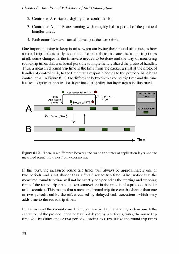
Chapter 8. Results and Validation of IAC Optimization
2. Controller A is started slightly after controller B.
3. Controller A and B are running with roughly half a period of the protocolhandler thread.
4. Both controllers are started (almost) at the same time.
One important thing to keep in mind when analyzing these round trip times, is howa round trip time actually is defined. To be able to measure the round trip timesat all, some changes in the firmware needed to be done and the way of measuringround trip times that was found possible to implement, utilized the protocol handler.Thus, a measured round trip time is the time from the packet arrival at the protocolhandler at controller A, to the time that a response comes to the protocol handler atcontroller A. In Figure 8.12, the difference between this round trip time and the timeit takes to go from application layer back to application layer again is illustrated.
Figure 8.12 There is a difference between the round trip times at application layer and themeasured round trip times from experiments.
In this way, the measured round trip times will always be approximately one ortwo periods and a bit shorter than a "real" round trip time. Also, notice that themeasured round trip time will not be exactly one period as the starting and stoppingtime of the round trip time is taken somewhere in the middle of a protocol handlertask execution. This means that a measured round trip time can be shorter than oneor two periods, unlike the effect caused by delayed task executions, which onlyadds time to the round trip times.
In the first and the second case, the hypothesis is that, depending on how much theexecution of the protocol handler task is delayed by interfering tasks, the round triptime will be either one or two periods, leading to a result like the round trip times
78

8.2 Simulation Accuracy
in Figure 8.5 - 8.6. In Figure 8.13 - 8.14 the two cases are explained.
The timing of the first case results in the round trip times always being one period onthe non-interfered controller. As seen in Figure 8.13 this is because there is alwaysenough time to not miss the execution of the protocol handler task, both from A toB and from B to A. However, if the protocol handler tasks are delayed "randomly"from interfering tasks, there are two different outcomes. If lucky, the delay causedby interfering tasks will not affect enough for the packet to miss a protocol handlertask execution. But if the protocol handler task execution is delayed a bit more in Athan it is delayed in B, the packet will miss the protocol handler task execution in Band will have to wait an extra period.
79

Chapter 8. Results and Validation of IAC Optimization
Figure 8.13 A timing diagram illustrating the behaviour when controller A is startedslightly before controller B. Depending on the timing of how the protocol handler task execu-tion may be delayed, different outcome in round trip times are retrieved. In the non-interferedcase, round trip times are always around one period. When other tasks interfere, the roundtrip times can be either of one period or two.
As illustrated in Figure 8.14, the behaviour in the second case is much like the onein the first case. Only here, an extra period will be added to the round trip timeif the protocol handler task is delayed more in B when receiving the request thanin a when the response is to be received. In this way, the packet must wait for theprotocol handler in controller A to execute before being sent to the application layer.
80

8.2 Simulation Accuracy
Figure 8.14 A timing diagram illustrating the behaviour when controller A is startedslightly after controller B. Depending on the timing of how the protocol handler task execu-tion may be delayed, different outcome in round trip times are retrieved. In the non-interferedcase, round trip times are always around one period. When other tasks interfere, the roundtrip times can be either of one period or two.
In the third case, interfering tasks will not affect the timing enough to make a dif-ference, thus, the round trip times will always be approximately one period long,that is 20 ms. As visualized in Figure 8.15, there is simply too much margin for thedelay caused by interfering tasks to have an impact on the system.
81

Chapter 8. Results and Validation of IAC Optimization
Figure 8.15 A timing diagram illustrating the behaviour when controller A and B arestarted one half of a period apart. Both in the non-interfered case and in the interfered case,round trip times are always around one period. Since the controllers are started one half ofa period apart, there is too much margin for the delays due to interfering tasks to have animpact on the system performance.
Finally, in the last case, the execution of the protocol handler task in both controllerswill occur at almost the same time, resulting in them always just missing the otherthread’s execution. As seen in Figure 8.16, this leads to round trip times of twoperiods, i.e. 40 ms. The reason that the randomness of the delays do not resultin some lucky round trip times in this case is because a system with the protocolhandlers in sync will also have the interfering tasks in sync. This makes the delaysin A and B the same as indicated by the dotted vertical lines in Figure 8.16.
82

8.2 Simulation Accuracy
Figure 8.16 The timing between the two controllers protocol handler threads when bothcontrollers start their protocol handler thread at the same time. Both with and without inter-fering tasks the round trip time will be about two periods long. The fact that this is the caseeven with interfering tasks, is due to that both controllers other tasks are timed identicallyand thus the delay caused by interfering tasks will always be the same for both A and B.
The explanations provided are just hypotheses. To get some support for the ideas,the phenomena were recreated in simulations. These simulations, unlike the onesused earlier, added the protocol handler threads to the controllers.
The first case was found using a setup where the Sensor/Actuator (Controller Ain the figures above) was started one ms before the Regulator (Controller B). Ahistogram of the round trip times from this setup with the unfiltered implementationof IAC is shown in Figure 8.17.
83
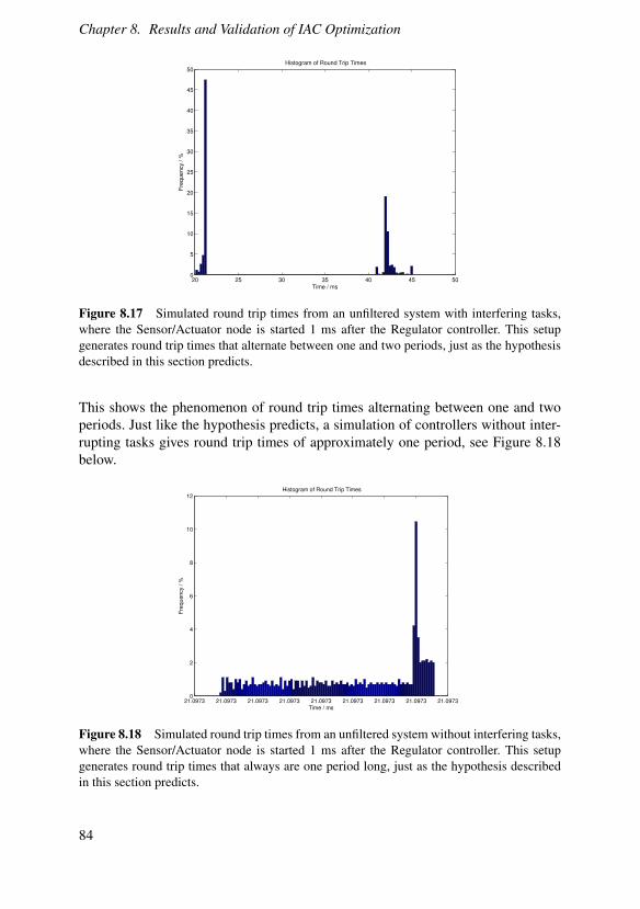
Chapter 8. Results and Validation of IAC Optimization
20 25 30 35 40 45 500
5
10
15
20
25
30
35
40
45
50Histogram of Round Trip Times
Time / ms
Fre
qu
en
cy /
%
Figure 8.17 Simulated round trip times from an unfiltered system with interfering tasks,where the Sensor/Actuator node is started 1 ms after the Regulator controller. This setupgenerates round trip times that alternate between one and two periods, just as the hypothesisdescribed in this section predicts.
This shows the phenomenon of round trip times alternating between one and twoperiods. Just like the hypothesis predicts, a simulation of controllers without inter-rupting tasks gives round trip times of approximately one period, see Figure 8.18below.
21.0973 21.0973 21.0973 21.0973 21.0973 21.0973 21.0973 21.0973 21.09730
2
4
6
8
10
12Histogram of Round Trip Times
Time / ms
Fre
quency / %
Figure 8.18 Simulated round trip times from an unfiltered system without interfering tasks,where the Sensor/Actuator node is started 1 ms after the Regulator controller. This setupgenerates round trip times that always are one period long, just as the hypothesis describedin this section predicts.
84

8.2 Simulation Accuracy
The same behaviour can be seen for the second case. In Figure 8.19, a histogram isshown using a setup with the Sensor/Actuator (Controller A) starting one ms afterthe Regulator (Controller B). Also, the simulation using non-interfered controllersgives round trip times of one period in this case as well.
20 25 30 35 40 450
5
10
15
20
25
30
35Histogram of Round Trip Times
Time / ms
Fre
qu
en
cy /
%
Figure 8.19 Simulated round trip times from an unfiltered system with interfering tasks,where the Sensor/Actuator node is started 1 ms before the Regulator controller. This setupgenerates round trip times that alternate between one and two periods, just as the hypothesisdescribed in this section predicts.
The hypothesis is once again confirmed in the third and the fourth case. Figure 8.20shows the round trip times of a system starting the controller one half of a periodapart. In Figure 8.21, the simulation results of a setup where the controllers arestarted at the same time are presented. Both setups use the unfiltered implementationand the non-interfered results are consistent with the hypotheses.
85

Chapter 8. Results and Validation of IAC Optimization
20 21 22 23 24 25 260
5
10
15
20
25
30
35
40
45
50Histogram of Round Trip Times
Time / ms
Fre
qu
en
cy /
%
Figure 8.20 Simulated round trip times from an unfiltered system with interfering tasks,where the two controllers are started with one half of a period apart. This setup generatesround trip times that always are one period long, just as the hypothesis described in thissection predicts.
40.5 41 41.5 42 42.5 43 43.5 44 44.5 45 45.50
5
10
15
20
25
30
35
40
45
50Histogram of Round Trip Times
Time / ms
Fre
quency / %
Figure 8.21 Simulated round trip times from an unfiltered system with interfering tasks,where the controllers are started at the same time. This setup generates round trip times thatalways are two periods long, just as the hypothesis described in this section predicts.
Given the results presented in this section, one can obtain high accuracy after ad-justing the simulation model. However, without prior knowledge about the system,the simulation model is usually rather poor and as a result, simulation data are notto be trusted.
86

8.3 Comparison to Current Implementation
8.3 Comparison to Current Implementation
As the results obtained from measurements show such varying behaviour, there isnot much to analyze regarding the efficiency of the IAC traffic filter. However, asthe adjusted simulation hopefully gives accurate results, a comparison between thefiltered and unfiltered implementations can be done.
The huge impact the periodic protocol handler thread has on the round trip timescannot be magically removed. Though, in the case of round trip times alternatingbetween one and two periods, as in case 1 and 2 described in the previous section,one might expect more "luck" resulting in more cases of one period round trip times.The simulated round trip times of a filtered versions corresponding to the systemsof Figure 8.17 and Figure 8.19 are shown in Figure 8.22 and Figure 8.23. Here itcan be seen that the systems using the same setup but with the filtered version ofIAC traffic handling, outperforms the systems using the unfiltered implementation.However, these are the only cases substantially benefiting from the filtered IACimplementation.
20 21 22 23 24 25 260
5
10
15
20
25
30
35
40
45
50Histogram of Round Trip Times
Time / ms
Fre
qu
en
cy /
%
Figure 8.22 Unlike the unfiltered version, this simulation data using filtered IAC trafficshows that round trip times in case 1 as defined in Section 8.2, using otherwise same settings,results in the round trip times always being one period long instead of alternating betweenone and two periods.
87

Chapter 8. Results and Validation of IAC Optimization
20 21 22 23 24 25 260
5
10
15
20
25
30
35
40
45
50Histogram of Round Trip Times
Time / ms
Fre
qu
en
cy /
%
Figure 8.23 Unlike the unfiltered version, this simulation data using filtered IAC trafficshows that round trip times in case 2 as defined in Section 8.2, using otherwise same settings,results in the round trip times always being one period long instead of alternating betweenone and two periods.
In practice, it is hard to validate the hypotheses and simulation results with mea-surements. This is due to the difficulties of controlling the starting times of thecontrollers manually. The controllers are restarted by pressing and holding a but-ton, so to systematically start controllers in a certain timing setup on purpose, e.g.one controller one ms before the other, is impossible. One could theoretically do avast amount of restarts of the systems randomly and take measurements from this,but in practice this would take way too much time and effort as the measurementtechnique used in this thesis has been partially manual.
88

9Conclusions
This chapter evaluates the results obtained in the thesis, as well as presenting someof the issues that were encountered during the workflow. In addition, possible futureimprovements are discussed.
9.1 Using TrueTime to Model 800xA
It has proven difficult to model a complex system as 800xA, as it requires a lotof knowledge of the system. The attempts on experimenting with different systemsettings in simulations, have resulted in insights regarding the effect packet lossprobability has on control systems using MMS and IAC protocols. However, othersimulation studies, e.g. experiments regarding RNRP, have been less rewarding.
Despite questionable gain of the studies done on overall system impact in this mas-ter’s thesis, the simulations of higher level protocols and controller timing behaviorhave been successful. As a consequence, the performed work can be used as a foun-dation for further studies of the 800xA system.
9.2 Optimizing IAC Traffic
Even though empirical evidence supporting the success of the optimized versionof IAC traffic handling has not been obtained, there are reasons to believe thatthe partially finished optimization has a performance boosting effect on the roundtrip times. This conclusion comes from the round trip times given by simulationdata. The reliability of the simulations is supported by the fact that simulated roundtrip times have been shown very similar to the experimental measurements, bothqualitatively and quantitatively.
The impact of shortened round trip times on overall system performance howeverremains unclear. This is heavily dependent on process characteristics and low leveltask timing behaviour in the controllers.
89

Chapter 9. Conclusions
9.3 Future Work
Unfortunately, time always limits what can be done in projects like this. Hence,ideas for future work are provided in this section.
Improvements to TrueTimeOne obvious disadvantage of using TrueTime compared to other network simula-tors, is its lack of support of standard higher level protocol such as TCP. A lot ofeffort was put on implementing the TCP protocol in the simulations, so integratingthis to the core of TrueTime would definitely be a nice feature.
Something that has not been mentioned in this master’s thesis, is the fact that the64-bit version of Matlab has some issues with TrueTime. This problem has beenavoided by using the 32-bit version of Matlab, but fixing this bug would be desir-able.
800xA SimulationsThe somewhat paradoxical fact of simulations, is that the simulation data is usuallybad and unreliable until a good model of the system is obtained. At the same time,simulation data is most valuable when there is not much knowledge about the sys-tem. The result of this is that the modeling and simulation of a system becomes aniterative process, where validation and analysis of an old simulation leads to modeladjustments and new simulation data. The new simulation results might give theusers better understanding of the system, making it possible to further adjust thesimulation model. This is the way the modeling of IAC round trip times was im-proved. This is also the way that every other aspect of the 800xA system simulationmodel can be enhanced. To sum up, almost endless future work can be spent onimproving the simulations of the 800xA system.
Expanding the IAC implementationThe optimized version of IAC traffic handling developed is limited to optimizingthe incoming IAC packets. Of course, it is preferred to optimize the packet routefor outgoing packets as well. However, the implementation of such an optimizationwould probably require a bit more effort than for the incoming packet optimization.This is because when sending a packet, information of where to send the packetmust be obtained. This is far from trivial in a system like 800xA, as the redundantnetwork requires the controller to keep track of its peers in the network. Getting thisinformation without going through the normal TCP/IP stack involves, for example,building routing tables.
Also, further investigations on the impact that shortened round trip times have on theoverall system performance is needed. This demands either a system setup mech-
90
9.3 Future Work
anism which is able to set the start times of the controllers in the network on atleast a millisecond scale, or large scale statistics of randomly started controllers.Furthermore, an analysis of how other threads in the controller are affected by thefilter thread should be done to prevent degrading system performance in other com-ponents.
91

Bibliography
ABB. System 800xA 5.1, Product Catalog (FP4 included). URL: http : / /www05 . abb . com / global / scot / scot354 . nsf / veritydisplay /a7dc1ca53bd960e2c1257b9d003d63a0 / $file / 3BSE062937 _ E _ en _System_800xA_5.1_Product_Catalog_(FP4_included).pdf.
ABB (2006). Industrial IT Compact Control Builder AC 800M Version 5.0 - GettingStarted Introduction and Installation.
ABB (2010). AC800M Communication Protocols.ABB (2012). System 800xA Network Configuration - System Version 5.1.ABB (2013a). DoF - Inter Application Communication.ABB (2013b). Fiedlbus and Network Communications. URL: http://www.abb.
se/product/us/9AAC115770.aspx.ABB (2013c). System 800xA - 5.1 AC 800M controller. URL: http : / /
www05 . abb . com / global / scot / scot400 . nsf / veritydisplay /39eb9295a4089dd5c1257c150052a1b6 / $file / 3BSE063691 _ D _ en _System_800xA_5.1_AC_800M_Controllers.pdf.
ABB (2013d). System 800xA I/Os. URL: http://www.abb.se/product/us/9AAC115771.aspx.
Cervin, A., D. Henriksson, B. Lincoln, J. Eker, and K.-E. Årzén (2003). “How DoesControl Timing Affect Performance? Analysis and Simulation of Timing UsingJitterbug and TrueTime.” IEEE Control Systems Magazine 23:3, pp. 16–30.
Cervin, A., D. Henriksson, and M. Ohlin (2010). TrueTime 2.0 beta 5 - ReferenceManual. Department of Automatic Control, Lund University.
Floyd, S. (1999). Validation Experiences with the NS Simulator. URL: http://www.icir.org/floyd/papers/NIST.Apr99.pdf.
Forouzan, B. A. (2013). Data Communcations and Networking. 5th. McGraw-Hill.Gkantsidis, C., M. Mihail, and E. Zegura (2003). The Markov Chain Simulation
Method for Generating Connected Power Law Random Graphs*. URL: http://www.siam.org/meetings/alenex03/Abstracts/CGkantsidis.pdf.
92

Bibliography
Information Science Institution (2011). The ns Manual. URL: http://www.isi.edu/nsnam/ns/doc/ns_doc.pdf.
J-Sim Homepage. URL: http://j-sim.cs.uiuc.edu/.ns-3 Homepage (2014). URL: https://www.nsnam.org/.ns-3 Project Goals (2006). URL: http://www.student.oulu.fi/~karivatj/
References/NS-3%20Project%20Goals.pdf.Omnet++ Homepage. URL: http://www.omnetpp.org/.Pan, J. (2008). A Survey of Network Simulation Tools: Current Status and Future
Developments. URL: http://www.cs.wustl.edu/~jain/cse567-08/ftp/simtools/index.html.
QualNet Homepage. URL: http://web.scalable-networks.com/content/qualnet.
REAL Homepage. URL: http : / / www . cs . cornell . edu / skeshav / real /overview.html.
Riverbed Homepage. URL: http : / / www . riverbed . com / products /performance-management-control/.
Rouse, M. (2012). Discrete Event Simulation (DES). URL: http : / / whatis .techtarget.com/definition/discrete-event-simulation-DES.
Sisco (1995). Overview and Introduction to the Manufacturing Message Specifica-tion (MMS). URL: http://www.sisconet.com/downloads/mmsovrlg.pdf.
SSFNet Homepage. URL: http://www.ssfnet.org/internetPage.html.tetcos (2014). Tetcos Homepage. URL: http://www.tetcos.com/.The ns-3 Manual (2014). URL: https://www.nsnam.org/docs/release/3.
19/manual/singlehtml/index.html.The OSI Model’s Seven Layers Defined and Functions Explained (2014).Waupotitsch, R., S. Eidenbenz, J. P. Smith, and L. Kroc (2006). MULTI-SCALE IN-
TEGRATED INFORMATION AND TELECOMMUNICATIONS SYSTEM (MI-ITS): FIRST RESULTS FROM A LARGE-SCALE END-TO-END NETWORKSIMULATOR. URL: http : / / www . cs . cornell . edu / ~kroc / pub /miitsWSC06.pdf.
93


Lund UniversityDepartment of Automatic ControlBox 118SE-221 00 Lund Sweden
Document nameMASTER´S THESISDate of issueJune 2014Document NumberISRN LUTFD2/TFRT--5949--SE
Author(s)
Viktor AnderssonTommi Nylander
SupervisorSven Gunnar Tiljander, ABBKarl-Erik Årzén, Dept. of Automatic Control, Lund University, Sweden (examiner)Sponsoring organization
Title and subtitle
Simulation of Process Control Network Traffic
Abstract
The majority of industrial control systems today are distributed over networks. These systems tend to be complex, and can be difficult both to configure and to analyze; therefore, there is definitely a gain in being able to simulate the behavior of such a system prior to the actual implementation.
This master’s thesis investigates the possibility to simulate the ABB automation system 800xA by expanding the Matlab/Simulink tool TrueTime. Throughout, the work has been focused on modeling the network communications and the internal behaviour of the control system nodes. Furthermore, the developed simulator has been used to examine a proposal to optimize traffic handling of the ABB specific protocol IAC.
Different performance measures have been investigated, both regarding control and network performance. One measure of particular interest has been the round trip time of a packet. The simulator has proven to be able to reproduce results of round trip times measured in an example system, explaining timing behaviour originating deep down in the control system nodes. Other simulations have involved different system settings, analyzing their impact on system performance.
Keywords
Classification system and/or index terms (if any)
Supplementary bibliographical information
ISSN and key title0280-5316
ISBN
LanguageEnglish
Number of pages1-93
Recipient’s notes
Security classification
http://www.control.lth.se/publications/


