Simulation of Legionella Concentration in Domestic Hot Water:

Comparison of Pipe and Boiler Models

Elisa Van Kenhovea*, Lien De Backerb, Arnold Janssensc and Jelle Laverged

a,b,c,dDepartment of Architecture and Urban Planning, Sint Pietersnieuwstraat 41 B4,

Ghent University, Ghent, Belgium

a*Elisa.VanKenhove@UGent.be, +32 (0)9 264 78 61, ORCID: 0000-0002-4648-0551

bLien.Debacker@UGent.be, -, ORCID: 0000-0002-0476-3537

cArnold.Janssens@UGent.be, +32 (0)9 264 39 06, ORCID: 30000-0003-4950-4704

dJelle.Laverge@UGent.be, +32 (0)9 264 37 49 , ORCID: 0000-0002-5334-1314

Simulation of Legionella Concentration in Domestic Hot Water:

Comparison of Pipe and Boiler Models

The energy needed for the production of domestic hot water represents an important

share in the total energy demand of well-insulated and airtight buildings. Domestic hot

water is produced, stored and distributed above 60°C to kill Legionella pneumophila.

This elevated temperature is not necessary for domestic hot water applications and has a

negative effect on the efficiency of hot water production units.

In this paper, system component models are developed/updated with L.

pneumophila growth equations. For that purpose different existing Modelica pipe and

boiler models are investigated to select useful models that could be extended with

equations for simulation of bacterial growth. In future research, HVAC designers will

be able to investigate the contamination risk for L. pneumophila in the design phase of a

hot water system, by implementing the customized pipe and boiler model in a hot water

system model. Additionally it will be possible, with simulations, to optimise

temperature regimes and estimate the energy saving potential without increasing

contamination risk.

Keywords: domestic hot water (DHW), Legionella pneumophila, pipe model, boiler

model, contamination risk, energy use

Introduction

Motivation

Domestic Hot Water (DHW) is an important building service in residential building

typologies such as dwellings, apartments, hotels, retirement homes, as well as in sports

facilities, hospitals, spas etc. (Stout and Muder, 2004).

Insulation levels and air tightness of building envelopes have been improved due

to the tightening of energy performance requirements for buildings. The production of

DHW, which has seen comparatively little innovation, now represents an important

share of total energy demand of well-insulated and airtight buildings (Rogatty, 2003).

On average, about 800kWh per occupant per year is the net energy needed for DHW

production (DIN 4708-2, 1994). For a dwelling with a floor area of 170m² and 3.5

occupants (Rogatty, 2003, Delghust et al., 2015), this amounts to 15kWh/m² a year.

This is the lowest (blue) bar in Figure 1. As can be seen in Figure 1, the total heating

demand for buildings built before 1984 (in Germany) is 225kWh/m² a year, this means

the energy needed for DHW accounts for about 6% of household energy costs, while for

passive buildings this is about 50%. Additional to the rising DHW energy use in

moderate or cold climates, warm climates have a limited heating demand which makes

the relative share in DHW energy demand equally large or even larger (Fuentes et al.,

2018).

Hot water energy demand remained unchanged over the years, while projected

energy performance requirements for 2020 state to reduce the total energy demand for

heating, cooling and DHW production to 1/3 of what they were in 2006.

Figure 1. Comparison of heating demand (ventilation, transmission and DHW) for

buildings of different age and energy efficiency level. The comparison is based on a

one-family house of 150m² (A/V=0.84) with three to four occupants in Germany

(adapted from Rogatty, 2003).

Problem statement

One of the main reasons for the high energy demand is that DHW is produced, stored

and distributed at temperatures above 60°C to mitigate the risk of contaminating the

DHW system with L. pneumophila. These bacteria cause, upon exposure, acute

respiratory disease or severe pneumonia. At temperatures above 60°C, L. pneumophila

growth is stopped and remaining bacteria are killed.

For most of the DHW applications, like taking a shower or washing hands,

temperatures of only 30-40°C are required. This disparity (between 60°C and 40°C),

doubles the temperature difference between DHW system and environment (around

20°C), which has a negative effect on distribution heat losses and on the efficiency of

DHW production units such as heat pumps. With the aim of more energy-efficient

buildings in mind, a straightforward strategy is to reduce temperature for hot water

production whenever possible (for certain periods). For that purpose, the growth of L.

pneumophila in systems needs to be known.

Ventilation heating demand (losses due to ventilation)Transmission heating demand (losses through the building envelope)Domestic hot water heating demand

Heating demand [kWh/(m²·yr)]240

200

160

120

80

40

0Building< 1984

Building1984-1994

Building> 1995

Low-energybuilding

Passivebuilding

50

50

4035

5

160

8050

3510

1515 15 15 15

Simulating L. pneumophila growth in DHW systems will result in a more

accurate prediction of the concentration of L. pneumophila in systems, which makes it

possible to investigate energy saving alternatives without increasing contamination risk.

State of the art

The 60°C temperature limit has been established by investigating the growth dynamics

of L. pneumophila bacteria in lab conditions and studying infected cases (Brundrett,

1992). No previous research has been published on modelling L. pneumophila on DHW

system level from a combined engineering-biological point of view. Recent studies

focus on the survival of Legionella bacteria and amoeba in biofilms (Konishi et al.,

2006, Buse et al., 2014). Other research projects look at the exposure mechanics once a

system is contaminated (Schoen et al., 2011, Hines et al., 2014) or focus on the

influence of tubing material (Van Der Kooij et al., 2005) etc. The literature about

decontamination strategies for contaminated systems is similarly scattered as that on the

proliferation of Legionella, usually focusing on a single decontamination technique and

tested in limited lab configurations or in case studies (Lehtola et al., 2005). The

limitations of these studies are summarized in Decontamination of Biological Agents

from Drinking Water Infrastructure (Szabo and Minamyer, 2014). Other papers focus

on the effect of these techniques on biofilms (Mathieu et al., 2014). Reports from

infection cases demonstrate that popular decontamination strategies such as applying

thermal shock or chlorination often only have a temporary effect. After returning to

normal use, Legionella growth resurfaces, probably due to flow stagnation or biofilm

residue. So far, accurate information on how to incorporate dynamic temperature

profiles, piping design or DHW use profiles in a risk assessment is not available,

limiting design options for DHW systems and forcing the available standards to require

high temperatures continuously. This is reflected for example in the REHVA

(Federation of European Heating, Ventilation and Air Conditioning Associations)

handbook on Legionella mitigation. Although a lot is known about the growth dynamics

of Legionella, and advances have been made in hydronic modelling allowing accurate

prediction of the dynamic flow conditions (temperatures, velocities, pressures) in DHW

systems (Vandenbulcke, 2013), both need to be combined in order to be able to assess

the L. pneumophila contamination risk on system level (Van Kenhove et al., 2015).

Scope

To build a simulation model, the possibilities to model L. pneumophila growth in water

and biofilm are investigated, and applied to pipe and boiler models.

In the first part of the paper, the theory, important to understand the simulation

model, is given. This includes the explanation of L. pneumophila growth in water and in

biofilm and ends with a figure of both growth curves, based on literature review data.

Next, the theory section is translated into a model, by curve fitting of the measurements

figure into temperature dependent growth equations. Mass conservation equations are

given for a typical pipe and storage tank component. Further, existing Modelica pipe

and storage tank components are compared and the most suitable one is chosen and

adapted by adding the growth equations. The paper ends with a proof of concept in

which the models are used to simulate a simple DHW system.

Methodology

A DHW system is composed of different components, for example pipes, storage tank,

heat exchanger, expansion vessel, taps. In this paper, system component models are

developed/updated with L. pneumophila growth equations. Based on water volume, the

main part of the system consists of piping and in most cases a storage tank. For that

purpose different existing Modelica pipe and boiler models are analysed to select useful

models that could be extended with equations for simulation of bacterial growth. After

selecting useful pipe and boiler models, these component models are chosen to be the

first to be adapted with the implementation of the L. pneumophila model, as growth and

exchange take mainly place in these components. The following paragraphs will show

how the chosen pipe and boiler model is adapted. However, following the same logic,

other Building Fluid elements for modelling thermohydraulic systems (e.g., expansion

vessel, pump, heat pump) can also be easily upgraded in the same way to include L.

pneumophila growth equations.

The benefit of modelling L. pneumophila growth in an existing pipe component

model is the ease of compiling simulation models of different systems later on by

dragging and dropping the different DHW components (which already include bacteria

growth equations) into the system model.

In future research, the customized pipe and boiler model can be implemented in

a hot water system model. This will make it possible to investigate the contamination

risk for L. pneumophila in the design phase of a DHW system, while keeping an

equilibrium between healthy buildings and energy efficiency, without compromising on

health. Additionally it will be possible, with simulations, to estimate the energy saving

potential without increasing contamination risk.

The growth curves in the simulation components are validated in this paper

based on literature data and the use of these components in different system simulation

models will be validated in future research based on test rig and case study

measurements.

Theory

In literature, there are no previous attempts to model the dependencies between L.

pneumophila growth and energy efficiency, probably because the topic requires a

multidisciplinary approach. This is the first time, to the authors’ knowledge, a dedicated

simulation model is made. The biological growth model is made up of a number of sub-

equations: growth and transport of L. pneumophila in water, L. pneumophila growth in

biofilm and bacteria transport between biofilm and water.

To model the proliferation of L. pneumophila in water, it is modelled as a trace

substance in different DHW components, for example a pipe and a boiler. Based on a

literature review, the main parameters that have an impact on the multiplication of L.

pneumophila bacteria are selected and added to the model as equations. This includes

the equations of dependency between L. pneumophila growth, water temperature and

flow conditions.

Legionella pneumophila growth in water

Multiplication of L. pneumophila is dependent on water temperature, volume flow rate,

flow frequency, followed by nutrient availability (Völker et al., 2015). At temperatures

below 20°C, the bacteria become dormant but remain viable for months. The bacteria

grow best at temperatures between 20°C and 45°C with an optimum around 35°C-41°C.

Beyond 45°C, pasteurization starts and higher temperatures will eventually kill the

organisms (Brundrett, 1992). This can be seen on Figure 2 and Figure 3. Figure 2 is

based on data from Yee and Wadowsky (1982) from experiments on unsterilized tap

water and Figure 3 is based on data from laboratory experiments (Dennis et al., 1984,

Stout et al., 1986, Schulze-Röbbecke et al., 1987, Sanden et al., 1989), and is consistent

with field data (Groothuis et al., 1985). On the x-axes, the water temperature in degrees

Celsius can be seen and on the y-axes, in Figure 2, the time to double the number of L.

pneumophila (mean generation time) and, in Figure 3, the time to reach 90% reduction

in cells (decimal reduction time). Figure 2 shows that the time to double the number of

L. pneumophila cells in water is less than half a day at 41°C and in Figure 3 it can be

noted that at 70°C, 90% of L. pneumophila in water gets killed in less than a minute.

The growth/death rate at any temperature is proportional to the number of living cells

present (Reddish, 1957, Sykes, 1965, Allwood and Russell, 1970) (Equation 1).

Growth/death rate: 𝑑𝐶(𝑡)

𝑑𝑡= 𝐴(𝑇) · 𝐶(𝑡) − 𝐵(𝑇) · 𝐶(𝑡) (1)

Number of cells: 𝐶(𝑡) = 𝐶0 · 𝑒(𝐴(𝑇)−𝐵(𝑇))·𝑡

With:

A(T) [-] Growth function depending on water temperature, the

species of the organism and the chemical nature of the

water

B(T) [-] Death function depending on water temperature, the species

of the organism and the chemical nature of the water

C0 [cfu/m³] Start concentration of L. pneumophila in water entering the

system

C(t) [cfu/m³] Concentration of L. pneumophila in water at time t

dC(t)/dt [cfu/s] Change in concentration of L. pneumophila over time

t [s] Time

Figure 2. An estimation of mean generation time (time to double the number of cells) of

L. pneumophila in tap water (data from Yee and Wadowsky, 1982, adapted from

Brundrett, 1992).

Figure 3. The change in decimal reduction time (90% reduction of L. pneumophila)

with temperature (data from Dennis et al., 1984, data from Stout et al., 1986, adapted

from Brundrett, 1992).

Legionella pneumophila growth in biofilm

An uncritical natural concentration of L. pneumophila enters the building, if the

conditions in these man-made environments are optimal for bacterial growth, it can

reach dangerous concentrations. If L. pneumophila would appear only in water, it would

Mean generation time [days]

Tap water temperature [°C]

5

4

3

2

1

020 25 30 35 40 45 50

Decimal reduction time (90% kill of Legionella) [h]

Tap water temperature [°C]

100

10

1

0.1

0.01

0.001

40 50 60 70 80

be flushed out of the system during water use and would not have time to grow.

However, DHW system component models do not only contain water, but also biofilm

(Figure 4).

What is a biofilm?

A biofilm is a slimy layer of microorganisms present inside for example water pipes.

This layer can be as thin as a single cell attached to the surface (<5μm) and as thick as

1 000μm (Murga et al., 1995).

Wherever there is water, biofilm growth can occur, for example in storage tanks,

humidifiers and cooling towers. Biofilms can grow easily in DHW pipes since they

provide a moist and warm environment for the biofilm to thrive. Modelling of the

biofilm is important because 95% of L. pneumophila are biofilm-associated (Flemming,

2002).

Figure 4. L. pneumophila in water (left graph with blue contour) and L. pneumophila

attached in biofilm (right graph with brown contour). The colors of these figures are

used throughout the paper to indicate in a quick visual way if a curve is obtained for

water or biofilm.

The biofilm structure is composed of a consortium of microbial cells that are attached to

the surface (substratum) and associated together in an extracellular anionic polymer

matrix (Donlan, 2002). The matrix is extremely hydrated (97% water) (Farhat et al.,

2012). Micro colonies of bacterial cells encased in the extracellular anionic polymer

matrix are separated from each other by interstitial water channels, allowing transport of

nutrients, oxygen, genes and even antimicrobial agents (Prakash et al., 2003). Because

of their dynamic character, biofilm communities can continuously change over time and

space, providing better survival and growth of the associated microorganisms

(Declerck, 2010). L. pneumophila bacteria attach to the biofilm because it consists of

microorganisms that allow cells to adhere to the pipe surface. Generally, there are three

distinct phases in the biofilm life cycle of L. pneumophila (Donlan, 2002): bacterial

attachment to a substratum, biofilm maturation and detachment from the biofilm, which

means dispersal in the bulk environment.

Protective function of the biofilm

The biofilm forms a protective layer for L. pneumophila that allows them to grow and

multiply within the biofilm. First, several authors have reported that L. pneumophila

bacteria living in a biofilm are more resistant to environmental stress and water

decontamination treatments (Fields et al., 1984, Sanderson et al., 1997, Sutherland,

2001, Russell, 2003, Borella et al., 2004, Van Der Kooij et al., 2005, Cervero-Aragó,

2015). This means for example a better resistance to higher temperatures. Secondly, L.

pneumophila is able to infect and replicate inside protozoans, which can survive as an

intracellular parasite of free-living amoebae (Rowbotham, 1980, Altschul et al., 1990,

Kilvington et al., 1990, Thomas et al., 2004, Wéry et al., 2008, Farhat et al., 2012).

Free-living amoebae are eukaryotic microorganisms that are commonly found in

drinking water systems, and more specifically in biofilms. This association established

between L. pneumophila and amoebae in biofilm in DHW systems indicates an

increased health risk because amoebae provide an ideal growth environment making L.

pneumophila bacteria more resistant to environmental stress and water decontamination

treatment.

Effect of temperature on Legionella pneumophila in biofilm

Cervero-Aragó et al. (2015) tested the effect of temperature on a L. pneumophila strain

and two amoebae strains under controlled laboratory conditions. To determine the

influence of the relationship between L. pneumophila and amoebae Acanthamoeba

species and Acanthamoeba Castellani on the treatment effectiveness, inactivation

models of the bacteria-associated amoeba were constructed and compared to the models

obtained for L. pneumophila living freely in water.

The thermal treatment was tested at four experimental temperatures: 50°C,

55°C, 60°C and 70°C, for various exposure times and applied to L. pneumophila under

controlled laboratory conditions. Table 1 lists the results and the R² values which show

the robustness of the regression models.

Table 1. Calculated time for a 4 log reduction of L. pneumophila serogroup 1

environmentally associated with Acanthamoeba Castellani CCAP 1534/2 and

Acanthamoeba species 155 after the exposure to different temperatures (adapted from

Cervero-Aragó et al., 2015).

Calculated time to reduce 4 logs [minutes]

Effect of temperature on free Legionella L. pneumophila sg. 1 env (Axenic) Effect of temperature on amoebae-associated Legionella L. pneumophila sg. 1 env - A. Castellani CCAP 1534/2 L. pneumophila sg. 1 env - Acanthamoeba sp. 155

50°C (R²) 46 (0.84)

50°C (R²) 825 (0.56) 664 (0.95)

55°C (R²) 8 (0.98)

55°C (R²) 45 (0.84) 51 (0.95)

60°C (R²) 4 (0.86)

60°C (R²) 5 (0.99) 5 (0.73)

70°C (R²) 0.61 (0.82)

70°C (R²) 0.45 (0.82) 0.50 (0.92)

The results in the upper section of Table 1 are comparable with the results of Figure 5

(blue curve). We are especially interested in the effect of temperature on L.

pneumophila inside amoebae, this can be seen in the lower section in Table 1. The

effectiveness of the thermal treatment on the amoebae-associated L. pneumophila

compared to the free living L. pneumophila was reduced. At 50°C, the L. pneumophila

resistance (measured in time) was increased 14 to 18 times, and at 55°C it was increased

5 to 6 times. Thus, it seems that Acanthamoeba and A. Castellani strains are protecting

L. pneumophila at temperatures below 60°C, but at higher temperatures, its protection

decreases enormously (Cervero-Aragó et al., 2015).

Figure 5 shows the temperature dependent growth function of L. pneumophila in

water (blue) and in biofilm (brown). The biofilm curve is an estimation established

based on the review results of available literature (Storey et al., 2004, Cervero-Aragó et

al., 2015). The study of Cervero-Aragó et al. (2015) shows the time required to reach a

4 log reduction for the Axenic L. pneumophila sg 1, when L. pneumophila was

associated with either Acanthamoeba or A. Castellani (in biofilm). The most negative

data (slowest death rate) of the Legionella-amoebae association is plotted into the

brown curve. There is no data available for the growth of L. pneumophila in biofilm

between 20 and 35°C. However, it is known from literature that the multiplication rate

of L. pneumophila, between 20°C and 30°C, is higher if it is present in biofilm

compared to water (Storey et al., 2004), but we cannot yet quantify it. Based on future

biological research this part of the growth curve can be replaced at a later stage.

Figure 5. Growth function of L. pneumophila in water (blue) (Brundrett, 1992) and in

biofilm (brown) (assumption derived from Storey et al., 2004, Cervero-Aragó et al.,

2015).

Dormant Multiplying Dying

Temperature [°C]

Multiplication of Legionella

Death rate of Legionella

10 20 30 40 60 70

Simulation and experiment

Modelling of Legionella pneumophila in DHW components

Figure 6 shows the modelling approach for L. pneumophila concentrations in pipe

models and Figure 7 in boiler models. The blue colour represents water, the brown

colour represents the biofilm.

Figure 6. Concentration of L. pneumophila in water (blue) and biofilm (brown) of DHW

pipe, shown as dual Control Volume (CV) scheme.

Figure 7. Concentration of L. pneumophila in water (blue) and biofilm (brown) of DHW

boiler, shown as dual CV scheme.

Cin(t)·Qin(t)Cb(t)·kc·Ab

C(t)·kc·Ab

Vb·mb(t)

Vp·m(t)

CV water

Cout(t)·Qout(t)

.

.

CV biofilm

Cin(t)·Qin(t)Cb(t)·kc·Ab

C(t)·kc·Ab

Vb·mb(t)

Vp·m(t)

Cout(t)·Qout(t)

.

.

To model L. pneumophila growth in water in a pipe or boiler, equations need to be

added to the hydraulic model. Following mass conservation equations, that predict L.

pneumophila growth in water, need to be coupled to an existing pipe or boiler

component (Equation 2, Equation 3, Equation 4).

𝑉𝑝 ·𝑑𝐶(𝑡)

𝑑𝑡= 𝐶𝑖𝑛(𝑡) ·

𝑄𝑖𝑛(𝑡)

𝜌− 𝐶𝑜𝑢𝑡(𝑡) ·

𝑄𝑜𝑢𝑡(𝑡)

𝜌+ 𝑔𝑟𝑜𝑤𝑡ℎ 𝑖𝑛 𝑤𝑎𝑡𝑒𝑟 +

𝑚𝑎𝑠𝑠 𝑡𝑟𝑎𝑛𝑠𝑓𝑒𝑟 𝑏𝑒𝑡𝑤𝑒𝑒𝑛 𝑤𝑎𝑡𝑒𝑟 𝑎𝑛𝑑 𝑏𝑖𝑜𝑓𝑖𝑙𝑚

𝑉𝑝 ·𝑑𝐶(𝑡)

𝑑𝑡= 𝐶𝑖𝑛(𝑡) · 𝐴𝑖𝑛 · �⃗�𝑖𝑛(𝑡) − 𝐶𝑜𝑢𝑡(𝑡) · 𝐴𝑜𝑢𝑡 · �⃗�𝑜𝑢𝑡(𝑡)

+ 𝑉𝑝 · �̇�(𝑡) + 𝑘𝑐 . 𝐴𝑏. (𝐶𝑏(𝑡) − 𝐶(𝑡)) (2)

𝑄𝑖𝑛(𝑡) = 𝑄𝑜𝑢𝑡(𝑡) (3)

�̇�(𝑡) = 𝐶𝑝𝑟𝑒𝑣𝑖𝑜𝑢𝑠 ·𝑙𝑛 (2)

𝑦· 𝑒

𝑙𝑛 (2)

𝑦·𝑑𝑡

(4)

With:

𝐴𝑏 [m²] Surface between water and biofilm

C(t) [cfu/m³] Concentration of L. pneumophila in water at time t

Cin(t) [cfu/m³] Concentration of L. pneumophila in water entering system

Cout(t) [cfu/m³] Concentration of L. pneumophila in water leaving system

Cb(t) [cfu/m³] Concentration of L. pneumophila in biofilm at time t

Cprevious [cfu/m³] Concentration of L. pneumophila in water on previous

timestep. Cprevious = Cb,0 on first timestep

dC(t)/dt [cfu/m³·s] Changing concentration of L. pneumophila over time

kc [m/s] Mass transfer coefficient to calculate the mass transfer of

L. pneumophila between water and biofilm

�̇�(t) [cfu/s] Change in concentration of L. pneumophila due to growth

or death

Qin(t) [kg/s] Mass flow rate of water (containing L. pneumophila)

entering system

Qout(t) [kg/s] Mass flow rate of water (containing L. pneumophila)

leaving system

T [K] Absolute temperature

t [s] Time

∆𝑡 [s] Timestep

Vp [m³] Volume of water in pipe or boiler

�⃗�𝑡 [m/s] Mass-average velocity for multicomponent mixture

y [s] Multiplication time of L. pneumophila in water dependent

on temperature

ρ [kg/m³] Mass density of mixture

To model L. pneumophila growth in biofilm in a pipe or boiler, equations need to be

added to the hydraulic model in a similar way as for growth in water. Following mass

conservation equations, that predict L. pneumophila growth in biofilm, need to be

coupled to an existing pipe or boiler component (Equation 5, Equation 6, Equation 7).

𝑉𝑏 ·𝑑𝐶𝑏(𝑡)

𝑑𝑡= 𝐶𝑏,𝑖𝑛(𝑡) ·

𝑄𝑏,𝑖𝑛(𝑡)

𝜌− 𝐶𝑏,𝑜𝑢𝑡(𝑡) ·

𝑄𝑏,𝑜𝑢𝑡(𝑡)

𝜌

+ 𝑔𝑟𝑜𝑤𝑡ℎ 𝑖𝑛 𝑏𝑖𝑜𝑓𝑖𝑙𝑚 + 𝑚𝑎𝑠𝑠 𝑡𝑟𝑎𝑛𝑠𝑓𝑒𝑟 𝑏𝑒𝑡𝑤𝑒𝑒𝑛 𝑏𝑖𝑜𝑓𝑖𝑙𝑚 𝑎𝑛𝑑 𝑤𝑎𝑡𝑒𝑟

𝑉𝑏 ·𝑑𝐶𝑏(𝑡)

𝑑𝑡= 𝐶𝑏,𝑖𝑛(𝑡) · 𝐴𝑏,𝑖𝑛 · �⃗�𝑏,𝑖𝑛(𝑡) − 𝐶𝑏,𝑜𝑢𝑡(𝑡) · 𝐴𝑏,𝑜𝑢𝑡 · �⃗�𝑏,𝑜𝑢𝑡(𝑡)

+𝑉𝑏 · �̇�𝑏(𝑡) + 𝑘𝑐 . 𝐴𝑏(𝐶(𝑡) − 𝐶𝑏(𝑡)) (5)

𝑄𝑏,𝑖𝑛(𝑡) = 𝑄𝑏,𝑜𝑢𝑡(𝑡) = 0 (6)

�̇�𝑏(𝑡) = 𝐶𝑏,𝑝𝑟𝑒𝑣𝑖𝑜𝑢𝑠 ·𝑙𝑛 (2)

𝑦𝑏· 𝑒

𝑙𝑛 (2)

𝑦𝑏·𝑑𝑡

(7)

With:

Ab [m²] Surface between biofilm and water

Cb(t) [cfu/m³] Concentration of L. pneumophila in biofilm at time t

Cin(t) [cfu/m³] Concentration of L. pneumophila in biofilm entering

biofilm segment

Cout(t) [cfu/m³] Concentration of L. pneumophila in biofilm leaving

biofilm segment

Cb,previous [cfu/m³] Concentration of L. pneumophila in biofilm on previous

timestep. Cb,previous = Cb,0 on first timestep

dCb(t)/dt [cfu/m³·s] Changing concentration of L. pneumophila in biofilm

over time

�̇�𝑏(𝑡) [cfu/m³·s] Change in concentration of L. pneumophila in biofilm due

to growth or death

Qb,in(t) [kg/s] Mass flow rate of water (containing L. pneumophila)

entering biofilm

Qb,out(t) [kg/s] Mass flow rate of water (containing L. pneumophila)

leaving biofilm

Vb [m³] Volume of biofilm in pipe or boiler

𝑣𝑏⃗⃗⃗⃗⃗(𝑡) [m/s] Mass-average velocity for multicomponent mixture

yb [s] Multiplication time of L. pneumophila in biofilm

dependent on temperature

As can be seen in Equation 6, mass flow between different biofilm segments is not

taken into account.

Determining multiplication time (y and yb)

The rate of increase of L. pneumophila is temperature dependent. Because it is

necessary to know the growth rate at every timestep, a function is created in Modelica

which returns the growth rate y and yb. Growth coefficient y is a time constant [s]

to predict growth or death of L. pneumophila in water. y in Equation 4 is dependent on

water temperature T in the pipe or boiler component. Equations of y are made for L.

pneumophila in water, based on a function that fits a polynomial through the defined

points in modelica, i.e., a vector containing temperature points and a vector containing

the corresponding concentration of L. pneumophila. The points are coming from the

curve presented in literature in Figure 2 and Figure 3, used with an interval of 1K as

shown in Annex 2 Table 10. Growth coefficient yb is a function to predict growth or

death of L. pneumophila in biofilm. yb in Equation 7 is dependent on water temperature

T in the pipe or boiler component. Growth coefficients are added for growth of L.

pneumophila in biofilm based on the results of Cervero-Aragó (2015). Annex 1

Equation 10 shows the equations of yb for L. pneumophila in biofilm, based on piece-

wise fitting of the curve in Figure 2 (growth) and measurement points presented in

literature and Table 1 (death).

A third degree piece-wise polynomial fitting technique (cubic hermite spline)

was chosen in Modelica for constructing a smooth curve through the defined points. In

total four different functions were developed: a separate function for the L. pneumophila

growth and death, each of them for L. pneumophila in water and for L. pneumophila in

biofilm. Several approaches have been tested, the current approach seems to have the

fewest drawbacks. The flexible use of the models is the reason to choose the current

approach. The advantage of using this approach, is that the user can easily adapt each

curve based on his own measurement points or new findings, or for another type of

bacteria.

Parameter Vb (volume of biofilm)

The parameter Vb in Equation 5 needs some more explanation. One of the difficulties

arising when taking the biofilm roughness into account is that a water pipe may be

smooth on installation and then progressively acquire a layer of calcium compounds

which make the surface rough and facilitate the growth of biofilm. The predicted human

contamination risk needs to be as low as possible, that is why the most negative

situation is modelled (biggest system contamination risk). For this purpose, a fully

developed biofilm is taken into account in the simulation models. The volume of

biofilm is a percentage of the pipe volume. This can be updated later on in function of

the pipe diameter. Although this simplification is made, it is important that the chosen

pipe and boiler models take material roughness into account, in this way the current

simplification can be updated by making biofilm thickness function of the pipes

roughness/pipe material.

Parameter kc (bacterial mass transfer coefficient)

Another parameter in the biologic model is the mass transfer coefficient kc. The

bacterial exchange between biofilm and the main water volume can be expressed with

the rate equation for convective mass transfer. This equation, generalized in a manner

analogous to Newton’s law of cooling, is (Welty et al., 2008):

𝑁𝐴 = 𝑘𝑐 · ∆𝑐𝐴

With:

𝑁𝐴 [mol/m²·s] Molar-mass flux of the species 𝐴, measured relative to

fixed spatial coordinates

∆𝑐𝐴 [mol/m³] Concentration difference between boundary surface

concentration and average concentration of diffusing

species in moving fluid stream

𝑘𝑐 [m/s] Convective mass-transfer coefficient

The method used to determine the mass transfer of bacteria between biofilm and water

is based on the boundary layer theory (Prandtl, 1904). The boundary layer is the thin

region of flow adjacent to the biofilm surface, where the flow velocity is dependent of

friction between the biofilm surface and the water (momentum boundary layer) and

where energy transfer (thermal boundary layer) and mass transfer (concentration

boundary layer) occur. The Reynolds analogy states that the mechanisms for transfer of

momentum and energy in the momentum and thermal boundary layer are identical if the

Prandtl number Pr equals 1 and that the momentum and thermal boundary layer

thickness are more or less equal. The Prandtl number for water is 4-7. In Welty et al.

(2008), this postulation is extended with mass transfer in case the Schmidt number Sc is

unity. For water however the Schmidt number is around 540. This Schmidt number

plays a role in convective mass transfer in the same way as the Prandtl number in

convective heat transfer. It can be expressed as the ratio of the molecular diffusivity of

momentum to the molecular diffusivity of mass. Using these analogies, a relation

between the different transport phenomena is expressed.

Since the Reynolds analogy is only valid for gases (Pr = 1 and Sc = 1), Chilton and

Colburn suggested an equation which makes it possible to extend the Reynolds analogy

to liquids by eliminating the restriction of unity of Prandtl and Schmidt numbers

(Colburn et al. 1933, Chilton et al., 1934). This analogy is valid for gases and liquids

within the range 0.6 ≤ Sc < 2 500. The convective mass transfer coefficient kc can be

obtained from the skin friction coefficient 𝐶𝑓 of the boundary layer and the Schmidt

number Sc:

𝑘𝑐

𝑣∞=

𝐶𝑓

2·

1

𝑆𝑐2/3

With 𝑣∞ [m/s] the velocity in the centre of the pipe.

For a laminar boundary layer, the skin friction coefficient was determined by Blasius

(1908).

𝐶𝑓 =1.328

√𝑅𝑒

For a turbulent boundary layer, different approximate solutions exist to calculate the

skin friction coefficient. In this work the Prandtl-Schlichting equation (Schlichting et

al., 1979), which uses a logarithmic velocity profile, is used. It is valid if Re < 109:

𝐶𝑓 = 0.455

(log𝑅𝑒)2.58

Parameter K (carrying capacity)

At certain critical temperatures, there is an unlimited increase of L. pneumophila

concentration in Equation 1 where in reality after a while a stabilization in

concentration will be noticed. This occurs because the system can only hold as many L.

pneumophila bacteria as nutrients and oxygen can support. To take nutrients into

account, parameter K, the carrying capacity, is added to the mass conservation equation

(Verhulst-Pearl logistic equation) (Panikov, 1995). It can be modelled with the

Verhulst-Pearl logistic equation, that is sigmoidal (S-shaped) and reaches an upper limit

at K. K is the maximum concentration of L. pneumophila that oxygen and nutrients can

support. L. pneumophila concentrations above K decline exponentially until they reach

the stable equilibrium K (Panikov, 1995) (Equation 8). The definition of A(T), B(T)

(Growth/death function depending on water temperature, the species of the organism

and the chemical nature of the water) can be seen in Equation 1.

𝑑𝐶(𝑡)

𝑑𝑡= 𝐴(𝑇) · 𝐶(𝑡) · (1 −

𝐶(𝑡)

𝐾) (growth)

𝑑𝐶(𝑡)

𝑑𝑡= 𝐵(𝑇) · 𝐶(𝑡) · (1 −

𝐶(𝑡)

𝐾) (death) (8)

To take K into account, Equation 4 and Equation 7 become Equation 4’ and Equation

7’ respectively.

�̇�(𝑡)

�̇�(𝑡)−𝐾 =

𝐶𝑝𝑟𝑒𝑣𝑖𝑜𝑢𝑠

𝐶𝑝𝑟𝑒𝑣𝑖𝑜𝑢𝑠−𝐾 · 𝑒

𝑙𝑛 (2)

𝑦·𝑑𝑡

(4’)

�̇�𝑏(𝑡)

�̇�𝑏(𝑡)−𝐾 =

𝐶𝑏,𝑝𝑟𝑒𝑣𝑖𝑜𝑢𝑠

𝐶𝑏,𝑝𝑟𝑒𝑣𝑖𝑜𝑢𝑠−𝐾 · 𝑒

𝑙𝑛 (2)

𝑦𝑏·𝑑𝑡

(7’)

To find the most suitable pipe and boiler component for this simulation purpose, a

comparative study is performed within the Modelica environment. First of all, a suitable

simulation environment and libraries are chosen. Subsequently, an adequate pipe and

boiler component is chosen.

Modelica simulation environment

Within the scope of this work, the following criteria were considered in first selecting

the simulation tool and secondly the components. These criteria are requirements for the

L. pneumophila growth model.

This is the first work to the authors’ knowledge that models L. pneumophila in

DHW systems. This means assumptions need to be made for some biological

parameters. As more biological research on these parameters is needed, this simulation

model can be considered as a framework for other researchers to overwrite the

assumptions. Therefore the modelling language should be open source and it should be

possible to adapt the code easily.

The goal is to have one tool that is flexible and that can be used for multiple

scales, from a whole building’s DHW system to L. pneumophila growth in a small

water/biofilm segment, and in multiple contexts, from design to decontamination.

Having a large number of different tools work together in such conditions is generally

perceived to be much less stable. Additionally, it requires the users to be acquainted

with all different simulation packages and is less flexible towards extensions of the

model to other situations.

Other boundary conditions are:

The model will be used in simulations of the DHW system of a building as a

whole or as a part of it. It is not necessary to model the building’s envelope and

other installation.

The modelling tool has to estimate short-term L. pneumophila growth (water

usage is second based), as well as long-term growth (effect of number of heat

shocks). In other words, it should be able to do a non-steady calculation of the

building’s DHW system for one day to one month (timestep of 0.1-1 second for

numerical stability).

The simulation tool has to be fast, the calculation of L. pneumophila growth

combined with one retrofitting option for a case study apartment building (of

200 apartments) with collective DHW system should be performed in maximum

24 hours. This is necessary to use the simulation model in decontamination

consultancy, where time is crucial.

It should be possible to perform the calculations on a ‘standard’ laptop (8GB

RAM - CPU 2 cores - 2.67 GHz). This is necessary to guarantee a broad use of

the simulation model in design and decontamination consultancy. For complex

systems, an exception can be made.

To meet these requirements, the simulation model is written in the Modelica language

and compiled in the Dymola environment (Modelica, 2016). This equation based

programming language is non-proprietary and object oriented. It also contains different

existing libraries, hydraulic as well as biologic, making it appropriate for the

development of multi-scale (thermohydraulic and biologic) models such as are required

here. This work adds to the capabilities of the Modelica models by providing a

biological growth library that was not available before. Modelica’s open source and

modular structure will allow users to use this library to model similar biological growth

problems in all kinds of applications.

Extensive libraries for simulation of buildings and their services have been

developed in IEA EBC Annex 60 (Annex 60, 2012). The Annex 60 integrated core

libraries are compatible with other Modelica building energy simulation libraries. For

this study existing pipe and boiler models of the standard Modelica (3.2.1) library and

of two libraries developed in Annex 60, namely OpenIDEAS (0.3.0) library and

integrated Buildings (3.0.0) library, are compared because all three libraries contain

building as well as system component models for energy performance simulation

(Wetter et al., 2014, Jorissen et al., 2018).

Comparison of pipe and boiler models in Modelica

There are a number of parameters necessary for modelling bacteria growth. The

parameters are divided into three categories, namely the three conservation equations:

mass conservation (differential continuity equation, Annex 3 Equation 31), momentum

conservation (Newton’s 2nd law of motion, Navier-Stokes equation, Annex 3 Equation

32) and energy conservation equation (Annex 3 Equation 33). It is studied how the

existing models deal with these conservation equations. The conversion from the

general form of the conservation equation to the equations with parameters used in the

Modelica simulation environment can be found in Annex 5. When referring to different

parameters below, the parameter names defined in Modelica are used.

To select the pipe and boiler models, following assumptions were made. First of

all, the pipe model has to be a 1D flow model, this means that the velocity in the x-

direction dominates the flow, meaning the velocity in y- and z-direction is negligible,

allowing the equations to be transformed to 1D. This means that CFD-models are not

considered. The second assumption made is that water is incompressible.

The mass conservation parameter ‘trace substances’ indicates if the existing pipe

component contains certain flow equations that make it possible to add substances to

water. This is the most important parameter related to the addition of L. pneumophila,

this is the parameter the growth equations need to be coupled with.

Momentum conservation parameter ‘gravity’ defines if the pipe can be used in

all directions (vertical/horizontal). A pipe model without inclusion of gravity can only

be used horizontally, except if the gravity equation is overruled by the pressure drop.

‘Pressure drop’ inclusion is important because it influences the fluid flow, which in

return influences mass transfer between biofilm and water. The momentum

conservation parameter ‘state of the flow (laminar/turbulent)’ is a meaningful parameter

for the purpose of this research because L. pneumophila growth is flow dependent, as

this influences the amount of bacteria attaching to and detaching from the biofilm into

the bulk liquid phase. Momentum conservation parameters like ‘friction’ and ‘material

roughness’ are important parameters in a pipe component because these parameters

influence the amount of biofilm formation.

Energy conservation parameters, for example the possibility to add a ‘heat

source’ and ‘insulation’, are meaningful parameters to take into account. They assure

that the pipe and boiler can be used in as many system configurations as possible.

‘nNodes’ means that the pipe can be divided into a predefined number of volume

segments. ‘Heat exchange’ is the exchange of heat with the environment. This is an

important part of the model to match real conditions as it influences water temperature,

which in its turn affects the growth or death of L. pneumophila bacteria.

It is not necessary to add other new parameters for bacteria growth to the

momentum and energy conservation equations, such as the parameter for L.

pneumophila growth added to the model in the mass conservation equation. However, it

is necessary to compare the inclusion of these parameters in the different models

because they are of interest for the growth equations and mass transfer between water

and biofilm (Equation 2 and Equation 5). For example, the volume of the biofilm

changes according to the material roughness. So material roughness should be

accessible as a parameter in the chosen pipe and boiler model.

Comparison of pipe models

Existing pipe models were compared based on the above parameters necessary for

modelling bacteria growth and that may or may not have been taken into account in the

conservation equations in the existing component models.

By comparing these parameters, the existing pipe models that can be extended

with equations for simulation of bacterial growth in DHW are selected. Table 2 gives an

overview of all selected existing pipe models (ranked according to the library to which

they belong) and the presence of the necessary parameters. If the parameter is indicated

by ‘1’ (green) it has been taken into account, if it is indicated by ‘0’ (red), the parameter

is not part of the existing model.

Out of the comparison of the different pipe models in Table 2, the authors chose

to adapt the ‘Pipe’ model from the Buildings (3.0.0) library because the most important

parameters are taken into account in the model. Gravity equations are missing from this

Pipe component, these can be added in a similar way as in the Dynamic pipe model.

However, it needs to be mentioned that the influence of adding this parameter is small

because for DHW applications, flow is dominated by pressure by using a pump

(parameter: pressure drop). Three other pipe models are suitable for the authors’

applications: Dynamic pipe, Insulated pipe and Pipe insulated. The reason not to retain

them is described in Annex 4.

Table 2. Comparison of DHW pipe component models based on parameters for bacteria growth modelling.

Data Mass

balance

Momentum

balance

Energy

balance Name Library Description Trace

substances

Gravity Pressure

drop

Laminar/

turbulent

flow

Friction Material

roughness

Heat

source

Heat

exchange

Insulation nNodes

Dynamic

pipe

Modelica

3.2.1

Dynamic pipe model

with storage of mass and

energy 1 1 1 1 1 1 0 1 0 1

Static pipe Modelica

3.2.1

Basic pipe flow model

without storage of mass

or energy 0 1 1 0 1 1 0 0 0 0

Heated

pipe

Modelica

3.2.1

Pipe with heat exchange 0 1 1 1 1 0 1 1 0 0

Isolated

pipe

Modelica

3.2.1

Pipe without heat

exchange 0 1 1 0 (only

laminar) 1 0 0 0 0 0

Short pipe Modelica

3.2.1

Simple pressure loss in

pipe 0 0 1 0 1 0 0 0 0 0

Embedded

pipe

OpenIDEAS

0.3.0

Embedded pipe model

based on prEN 15377

and (Koschenz, 2000) 1 0 1 1 1 1 0 1 1 0

Insulated

pipe

OpenIDEAS

0.3.0

Insulated pipe

characterized by UA 1 0 1 1 1 0 0 1 1 0

Pipe OpenIDEAS

0.3.0

Pipe without heat

exchange or pressure

drop 1 0 0 0 0 0 0 0 0 0

Pipe

heatport

OpenIDEAS

0.3.0

Pipe with HeatPort 1 0 1 1 1 0 0 1 0 0

Pipe

insulated

OpenIDEAS

0.3.0

Pipe with insulation,

characterized by UA 1 0 1 1 1 0 0 1 1 0

Lossless

pipe

OpenIDEAS/

Buildings

3.0.0

Pipe with no flow

friction and no heat

transfer 0 0 0 0 0 0 0 0 0 0

Pipe Buildings

3.0.0

Pipe with finite volume

discretization along flow

path 1 0 1 1 1 1 0

1

(multiple

heat ports)

1 1

Comparison of boiler models

Next to pipe models, existing boiler models were compared based on the parameters for

bacteria growth modelling. In case of boilers an additional parameter which is important

for modelling the growth and displacement of L. pneumophila is ‘stratification of the

boiler’.

Table 3 gives an overview of all selected existing boiler models, the library to

which they belong and the presence of the necessary parameters. If the parameter is

indicated by ‘1’ (green) it is taken into account, if it is indicated by ‘0’ (red), the

parameter is not part of the existing model.

Out of the comparison of the different boiler models in Table 3, the

‘StratifiedEnhancedInternalHex’ boiler model, of the Buildings library 5.0.1, is chosen

as most suitable for the authors’ applications because it meets most of the requirements

and is a stratifying boiler. As well as the Pipe model, it contains a Mixing Volume

component which will be used to implement the growth equations (see Implementation).

Reasons why not to retain certain other models are mentioned in Annex 4.

Other DHW components, like heat exchangers, expansion vessels, water

softeners etc. are not, but the modelling approach is similar.

Table 3. Comparison of DHW boiler component models based on parameters for bacteria growth modelling.

Data Mass

balance

Momentum

balance

Energy

balance

Strati-

fication Name Library Description Trace

substances

Gravity Pressure

drop

Laminar/

turbulent

flow

Friction Material

roughness

Heat

source

Heat

exchange

Insulation nNodes

Boiler OpenIDEAS

0.3.0

Modulating boiler with

losses to environment,

based on performance

tables 1 0 1 1 0 0 1 1 0 0 0

Boiler

Polynomial

Buildings

3.0.0

Boiler with efficiency

curve described by a

polynomial of the

temperature 1 0 1 1 0 0 1 1 1 0 0

OpenTank Modelica

3.2.1

Simple tank with

inlet/outlet ports 1 0 1 1 0 0 0 1 0 0 0

Storage

Tank

OpenIDEAS

0.3.0

1D multinode stratified

storage tank 0 0 0 0 0 0 0 1 1 1 1

Storage

Tank_One

IntHX

OpenIDEAS

0.3.0

1D multinode stratified

storage tank with one

internal heat exchanger

(HX) 0 0 0 0 0 0 1 1 1 1 1

Stratified

Enhanced

Internal

Hex

Buildings

3.0.0

A model of a water

storage tank with a

secondary loop and

internal heat exchanger 1 0 1 1 1 0 1 1 1 1 1

Implementation of Legionella pneumophila equations

Medium with Legionella pneumophila and nutrients

Modelica has a modular approach, meaning that a whole DHW system is modelled by

connecting several components. A Medium flows through the different components.

The Buildings Fluid components make use of a Mixing Volume, equivalent to a Control

Volume (CV) with a replaceable Medium. For this application a new Medium is defined

starting from the Buildings.Media.Water to which two trace substances are added,

namely L. pneumophila and nutrients. By doing so, two additional mass conservation

equations are added. This updated Medium has to be used in every component of the

simulated hydraulic system.

Modelica library with L. pneumophila growth and nutrients models

However, the addition of two trace substances (L. pneumophila and nutrients) to the

Medium water are not sufficient to calculate the L. pneumophila concentration in a

hydraulic system as the growth and mass transfer equations (Equation 2, Equation 5)

are not included.

Therefore, a new library is developed consisting of new functions, models and

extended components to predict L. pneumophila growth. Equations have to be added to

include the L. pneumophila growth in water/biofilm and the mass exchange between

water and biofilm. To include the necessary equations, two new models are developed:

one including equations for the concentration of L. pneumophila (upper icon highlighted

in yellow in Figure 8 and Figure 9) and one including equations for the concentration of

nutrients (lower icon highlighted in yellow in Figure 8 and Figure 9). By implementing

the L. pneumophila and nutrients model as a partial model and by extending the original

models of the component models, flexible use of the model is allowed. Moreover, it is

implemented in such a way, that computation of L. pneumophila could be conditionally

disabled. Additionally, in case the user wants to calculate more or other concentrations,

equations could be added in the same way.

Pipe model implementation

Figure 8 shows the modification of the customized Pipe model from the Buildings

(3.0.0) library. Figure 8A demonstrates the visual representation of the customized pipe

element (icon view). The brown rectangles visually represent the addition of biofilm

and the black circles the exchange of bacteria between biofilm and water. Figure 8B,

showing the diagram view of the pipe, illustrates how the original Pipe model is adapted

to include the thermohydraulic and biologic equations. As can be noticed, the new L.

pneumophila and nutrients models described above are added to the pipe model of the

Buildings Fluid library. These models contain Equations 2-8. For someone unfamiliar

with the Modelica modeling software, an explanation of each symbol used in Figure 8B

is given in Annex 5 Table 11. Additionally, an explanation of each equation used behind

Figure 8B and the conversion from the theoretical continuity equation to the

implementation of equations in Modelica is given in Annex 3 and Annex 5.

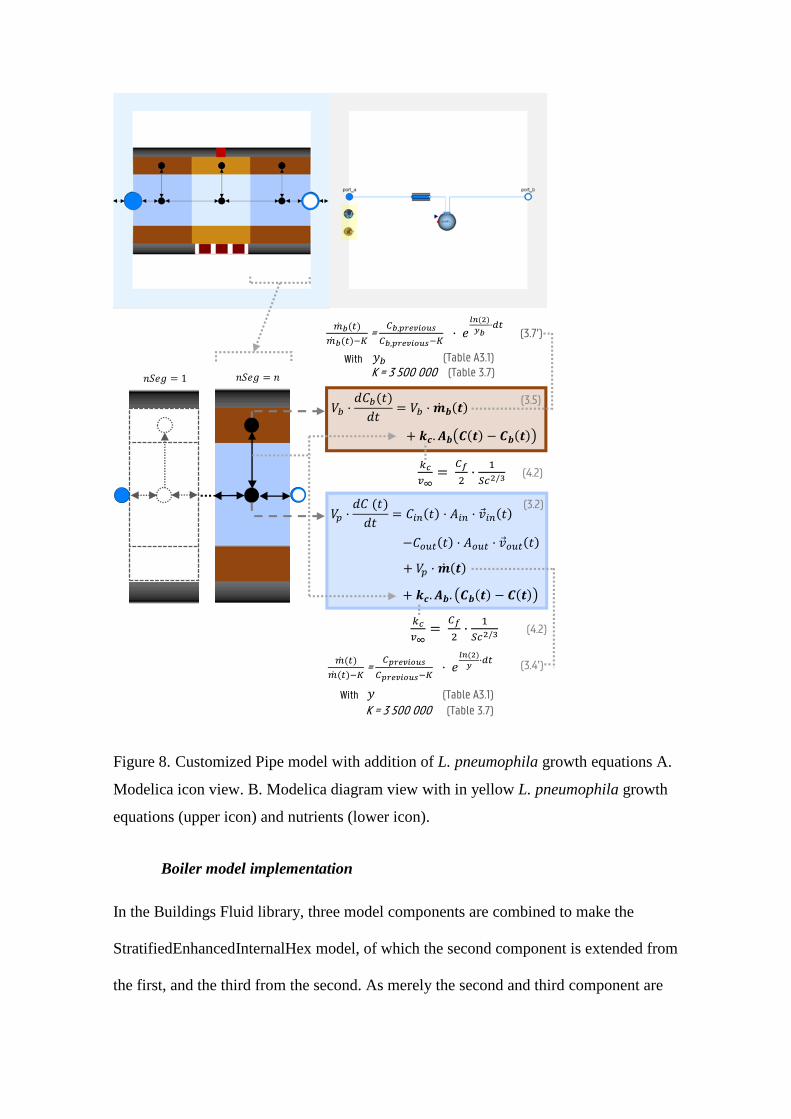
Figure 8. Customized Pipe model with addition of L. pneumophila growth equations A.

Modelica icon view. B. Modelica diagram view with in yellow L. pneumophila growth

equations (upper icon) and nutrients (lower icon).

Boiler model implementation

In the Buildings Fluid library, three model components are combined to make the

StratifiedEnhancedInternalHex model, of which the second component is extended from

the first, and the third from the second. As merely the second and third component are

(3.5)𝑉𝑏 ·

𝑑𝐶𝑏(𝑡)

𝑑𝑡= 𝑉𝑏 · ̇

+ . −

�̇�𝑏(𝑡)

�̇�𝑏(𝑡)−𝐾=

𝐶𝑏,𝑝𝑟𝑒𝑣𝑖𝑜𝑢𝑠

𝐶𝑏,𝑝𝑟𝑒𝑣𝑖𝑜𝑢𝑠−𝐾 · 𝑒

𝑙𝑛 (2)

𝑦𝑏·𝑑𝑡

(3.7’)

𝑏 (Table A3.1)K = 3 500 000 (Table 3.7)

With

𝑛 𝑒𝑔 = 1 𝑛 𝑒𝑔 = 𝑛

𝑉𝑝 ·𝑑𝐶 (𝑡)

𝑑𝑡= 𝐶𝑖𝑛 𝑡 · 𝐴𝑖𝑛 · �⃗�𝑖𝑛 𝑡

−𝐶𝑜𝑢𝑡 𝑡 · 𝐴𝑜𝑢𝑡 · �⃗�𝑜𝑢𝑡 𝑡

+ 𝑉𝑝 · ̇

+ . . −

(3.2)

𝑘𝑐

𝑣∞=

𝐶𝑓

2·

1

𝑆𝑐2/3 (4.2)

With

K = 3 500 000

�̇�(𝑡)

�̇�(𝑡)−𝐾=

𝐶𝑝𝑟𝑒𝑣𝑖𝑜𝑢𝑠

𝐶𝑝𝑟𝑒𝑣𝑖𝑜𝑢𝑠−𝐾 · 𝑒

𝑙𝑛 (2)

𝑦·𝑑𝑡

(Table A3.1)(Table 3.7)

(3.4’)

𝑘𝑐

𝑣∞=

𝐶𝑓

2·

1

𝑆𝑐2/3 (4.2)

used, the second component is adapted, and automatically the third component is

adapted as this extends from the second one.

The modification of the retained StratifiedEnhancedInternalHex model (third

component) from the Buildings (3.0.0) library can be seen in Figure 9. Figure 9A shows

the visual representation of the customized model (icon view). The brown rectangles

visually represent the addition of biofilm and the black circles the exchange of bacteria

between biofilm and water. Figure 9B shows the thermohydraulic and biologic

adaptation of the retained boiler model. Equations 2-12 are written in this model (in

yellow). Figure 9B is explained in more detail in Annex 5 Table 11. Additionally, an

explanation of each equation used behind Error! Reference source not found.B and the

conversion from the theoretical continuity equation to the implementation of equations

in Modelica is given in Annex 3 and Annex 5.

Figure 9. Customized StratifiedEnhancedInternalHex boiler model with addition of L.

pneumophila growth equations. A. Modelica icon view. B. Modelica diagram view with

in yellow L. pneumophila growth equations (upper icon) and nutrients (lower icon).

Computational costs

To give an indication of how the inclusion of the L. pneumophila model in the pipe and

boiler element affects the numerical efficiency of the Modelica models, several aspects,

such as the number of variables, number of time and state events and CPU time, are

compared in Table 4, 0 and Table 6. In Table 4 the pipe and boiler component are used

with and without the addition of the equations to calculate the L. pneumophila growth.

Equations are divided into nontrivial and trivial equations. Trivial equations are simple

equations from which you can immediately find the unknown. For nontrivial equations,

a more difficult solution method must be applied (e.g., an iteration method). In 0 and

Table 6 the computational costs are presented for the pipe and the boiler component.

More explanation to understand the simulation log basics is given in Annex 6 Table 16.

The required solver is Euler because of the use of spatial and time discretization in the

growth models. The simulation parameters used are:

Solver Euler (explicit)

Timestep 0.1s

Tolerance 0.0001

Number of pipe segments 2

Number of boiler segments 8

Table 4. Statistical analyses of the pipe and boiler component model with and without

L. pneumophila growth equations.

Number of… Pipe model without

Legionella

Pipe model with

Legionella

Difference

Components

Variables

Constants

Parameters

Unknowns

Differentiated variables

76

828

12

388

428

14

79

908

12

421

475

18

3

80

0

33

47

4

Equations

Nontrivial

Trivial

339

249

90

376

278

103

37

29

13

Number of… Boiler model without

Legionella

Boiler model with

Legionella

Difference

Components

Variables

Constants

Parameters

Unknowns

Differentiated variables

Equations

Nontrivial

Trivial

172

2 160

31

763

1 366

39

913

669

250

176

2 256

31

795

1 430

55

943

686

257

4

96

0

32

64

16

30

23

7

Table 5. Comparison of computational costs of the pipe component model with and

without L. pneumophila growth equations.

Pipe model without Legionella Pipe model with Legionella

CPU-time for integration

CPU-time for one GRID interval

Number of result points

Number of GRID points

Number of (successful) steps

Number of F-evaluations

Number of H-evaluations

Number of Jacobian-evaluations

Number of (model) time events

Number of (U) time events

Number of state events

Number of step events

Minimum integration stepsize

Maximum integration stepsize

Maximum integration order

16.9s

0.90ms

189

189

564 000

564 000

564 001

0

56 399

0

0

0

0.1

0.1

1

CPU-time for integration

CPU-time for one GRID interval

Number of result points

Number of GRID points

Number of (successful) steps

Number of F-evaluations

Number of H-evaluations

Number of Jacobian-evaluations

Number of (model) time events

Number of (U) time events

Number of state events

Number of step events

Minimum integration stepsize

Maximum integration stepsize

Maximum integration order

39.9s

2.12ms

189

189

564 000

564 000

564 005

0

56 399

0

4

0

0.1

0.1

1

Table 6. Comparison of computational costs of the boiler component model with and

without L. pneumophila growth equations.

Boiler model without Legionella Boiler model with Legionella

CPU-time for integration

CPU-time for one GRID interval

Number of result points

Number of GRID points

Number of (successful) steps

Number of F-evaluations

Number of H-evaluations

Number of Jacobian-evaluations

Number of (model) time events

Number of (U) time events

Number of state events

Number of step events

26.7s

53.4ms

113 201

501

564 707

6 154 908

621 507

508 195

56 399

0

0

0

CPU-time for integration

CPU-time for one GRID interval

Number of result points

Number of GRID points

Number of (successful) steps

Number of F-evaluations

Number of H-evaluations

Number of Jacobian-evaluations

Number of (model) time events

Number of (U) time events

Number of state events

Number of step events

157s

2.79ms

130 936

56 401

564 000

564 000

573 069

0

56 399

0

9 068

0

Minimum integration stepsize

Maximum integration stepsize

Maximum integration order

0.0002

0.489

2

Minimum integration stepsize

Maximum integration stepsize

Maximum integration order

0.1

0.1

1

Summary of simulation model assumptions

Although fragmentary mentioned throughout the paper, an overview of all simulation

model assumptions is given below.

Component models assumptions

The three conservation equations are part of the DHW system component models (e.g.,

pipe, boiler): the law of conservation of mass (mass continuity equation), the first law of

thermodynamics on energy conservation (energy equation) and Newton’s second law of

motion (momentum theorem) with pressure loss calculated with the Swamee-Jain

equation, which is based on the Colebrook-White equation.

The L. pneumophila growth equations are added to the component models in the

mass conservation equation. A dual control volume approach has been followed for

water and biofilm. For the momentum and energy conservation equation, water and

biofilm are considered as one node. This means that the temperature in the biofilm is

assumed to be the same as the water temperature, which is correct for an insulated

system. No separate velocity profile has been assumed in the biofilm.

The pipe model used is based on the finite volume method. Every pipe

component is subdivided in nSeg nodes. Perfect mixing of water is assumed in every

node. Flow reversal (back flow) is taken into account in the pipe model, based on

pressure differences. Advection is included in two directions.

Diffusion between two water segments, in a pipe model and in between pipe

models, is not taken into account in any Modelica pipe model as it is not part of the

existing mass conservation equations in the underlying MixingVolume model in

Modelica. It should be possible to add this in future, but as for now reuse of the L.

pneumophila model in different existing system component models is aimed for,

meaning that it is necessary to use the existing mass conservation equation instead of

replacing it in all components. Neglecting diffusion between different pipe segments

can be done, as the model is used for systems with mainly continuous circulation, it is

assumed that advection is much larger than diffusion. Only if stagnation occurs,

diffusion can become important. Therefore an alternative T-section has been made to

include diffusion from a distal pipe to the primary recirculation circuit. Diffusion

between biofilm and water and thermal diffusion in the boiler are taken into account.

Water assumptions

The density of the medium is temperature dependent and the presence of L.

pneumophila bacteria is not influencing the density of the mixture.

Nutrients K are coupled to the mass conservation equation, meaning that they

are distributed by water flowing through the system, but no growth or decay equations

for nutrients are coupled to this mass conservation equation. Nutrients are considered to

be present in excess. This assumption is correct for systems with regular use, because a

stock of nutrients is continuously entering the system. In reality, if water would stand

still for a very long time, there would be no nutrient entering, meaning that L.

pneumophila would die because of the lack of nutrients. However, literature confirms

that L. pneumophila is found in systems without fresh nutrients after periods of two

years (Garduno et al. 2002, Robertson et al. 2014, Al-Bana et al. 2014). If in future

quantitative information on the relation between L. pneumophila and nutrients is

available, it will be possible to add it to the model. However, in the current real system

simulations with regular hot water use, the carrying capacity K is not reached by far, so

a lower value of K would not change the results. In this case, the most critical situation

is modelled. Additionally, no active movement of bacteria based on nutrients is taken

into account, meaning bacteria are not moving to areas with higher nutrient

concentrations.

Biofilm assumptions

A fully grown biofilm is taken into account. The biofilm thickness is a parameter that

cannot be measured easily. Based on discussions with biofilm experts (Biofilm

conference, 2017), a cut-off value for the thickness has been assumed. The biofilm

thickness is a function of the diameter of the pipe or boiler. The thickness of the biofilm

is calculated based on the percentage of the volume. The biofilm thickness has been

subtracted from the diameter to calculate the wall surface of a pipe or boiler. In the

boiler, an extra condition has been added, namely that the thickness of biofilm on the

bottom of the boiler is five times the thickness of the biofilm on the surface. If for a

certain case the thickness of the biofilm would be known, it could be added to the model

in one parameter.

The spatial structure of the biofilm is not taken into account due to the lack of

literature data. Local vortexes are not taken into account, as the mass transfer coefficient

kc is fixed. The mass transfer coefficient kc between biofilm and water is function of the

flow velocity and the concentration difference between biofilm and water.

A biofilm is thicker in pipes with a larger diameter, this can be explained by the

speed profile in a pipe. The surface biofilm area of the boiler does not include the area

of the heating elements inside. The volume of biofilm is considered to be divided over

the wall’s surface area. In future, it could be better to divide the volume over all surface

elements.

Flow in between different biofilm segments is not taken into account, as

literature shows that biofilms formed above 37°C have no water channels within

(Mampel et al., 2006).

Result analysis

Proof of concept - simple domestic hot water system configuration

The Buildings (3.0.0) pipe and boiler model, with addition of L. pneumophila growth

equations in water and biofilm, can now be used to build different DHW system

configurations. The most simple system configuration is represented in Figure 10. This

system contains a boiler with internal heat exchanger, the upper side of the boiler is

connected to a pipe and a tap profile.

Figure 10. Simple DHW system with customized boiler and pipe components.

Initial model values are assigned to the biological parameters based on measurements,

calculations, material characteristics and review of available literature. These parameter

values are displayed in Table 7.

Table 7. Initial biological model parameter values (Brundrett 1992, Cervero-Aragó et al.

2015, Biofilm conference 2017, Van Kenhove et al. 2018)

Component Modelling

challenge

Parameter Source for

initial value

Initial model

value

Boiler Start concentration

of Legionella

Cstart

[cfu/m³]

Cold water

concentration

25

Volume of biofilm Volume [m³] Literature review Vtank/10

Roughness [m] Material

characteristics

Smooth steel:

0.000025

Pipes Start concentration

of Legionella

Cstart

[cfu/m³]

Cold water

concentration

25

Volume of biofilm Volume [m³] Literature review Vpipe/10

Roughness [m] Material

characteristics

Smooth steel:

0.000025

Component

independent

Mass transfer

coefficient

[m/s] Calculation 𝑘𝑐 =𝐶𝑓

2· v∞

Re < 3500:

𝐶𝑓 =1.328

√𝑅𝑒

Re > 3500:

𝐶𝑓 =0.455

log(Re)2.58

Growth equation of

Legionella in water

[cfu/m³] Literature review Water curve

Growth equation of

Legionella in biofilm

[cfu/m³] Literature review

+ measurements

Biofilm curve

Nutrients [cfu/m³

=> kg/m³]

Literature review

+ measurements

3 500 000 000

The hydraulic parameters which need to be defined by the user, are the same parameters

as in the standard Pipe and StratifiedEnhancedInternalHex boiler model. Default values

for these parameters are suggested by the developers of the Modelica components. The

following parameter conditions are chosen to run the simulation of the system presented

in Figure 10:

length 20m (Length of pipe)

diameter 0.05m (Diameter without insulation)

dIns 0m (Insulation thickness of pipe)

lambdaIns 0.026W/m·K (Lambda value of insulation)

nSeg pipe 2 (Number of volume segments)

nSeg boiler 8 (Number of volume segments)

m_flow_nominal 0.0016kg/s (Nominal mass flow rate)

dp_nominal 0.5Pa (Pressure difference)

The simulation setup is chosen as follows:

start time 0s

stop time 86 400s

integration algorithm Euler (explicit)

integration tolerance 0.0001

timestep 0.1s

The simulation output is the following:

Predicted L. pneumophila concentration in the pipe (pipe.vol[1].C) as in Figure

11 (translated into Figure 12 and Figure 13), Figure 14 and Figure 15.

Predicted L. pneumophila concentration at the outlet of the pipe

(pipe.port_b.C_outflow[1]) as in Figure 16.

Verification exercise - reproducing growth time curves

To verify the growth time curves as in Figure 2 (growth) and Figure 3 (starvation), a

similar temperature profile is imposed on the simulation model, namely a production

temperature linearly rising from 25°C to 80°C. The predicted L. pneumophila

concentration in Figure 11 (concentration in function of temperature) is translated into

Figure 12 (growth-time curves). The predicted L. pneumophila concentrations in Figure

12, by simulating the system of Figure 10, show similar behaviour as in Figure 2 and

Figure 3. The same can be noticed from the growth/death curves of L. pneumophila in

biofilm (Figure 13) based on the results of Table 1. RMSE of around 0 and R² of around

1 (cannot be expressed more accurately as the authors do not have the measurement

data behind the curves, except from the visual appearance) are achieved between

measurement points (black line) and simulation results (blue dotted line) because the

measurement points are the inputs used in the component models.

Figure 11. Predicted L. pneumophila concentration in pipe in function of outlet

temperature.

Figure 12. A. Simulation of mean generation time (time to double the number of cells)

of L. pneumophila in water at different temperatures (blue dotted line: simulation result,

black line: measurements from Figure 2). B. Simulation of the change in decimal

reduction time (90% reduction in L. pneumophila in water) at different temperatures

(similar to Figure 3).

Legionella pneum. concentration [cfu/l]

Time [h]

40

35

30

25

20

15

10

5

0

80

70

60

50

40

30

20

10

00 2 4 6 8 10 12 14 16 18 20 22 24 26 28 30 32

Temperature [°C]

Mean generationtime [days]

5

4

3

2

1

020 25 30 35 40 45

Decimal reduction time(90% kill of Legionella) [h]

Tap water temperature [°C]

100

10

1

0.1

0.01

0.00140 50 60 70 80

Figure 13. A. Simulation of mean generation time (time to double the number of cells)

of L. pneumophila in biofilm (brown dotted line: simulation result, black line:

measurements from Figure 2). B. Simulation of change in time to reduce 4 logs with

temperature.

Sensitivity analyses

The robustness of the adapted component models is tested by running some simulations

on the simple system presented in Figure 10, to assess the influence of several variables

on the growth of L. pneumophila.

As seen before, L. pneumophila growth is dependent on temperature and mass

flow rate. Figure 14 shows the influence of the flow rate at a constant ideal growth

temperature of 40°C. The biologic and hydraulic parameters are the same as before,

only the mass flow rate is varied. A constant tap profile is implemented which is the

same as the mass flow rate. Figure 14 shows the concentration of L. pneumophila in the

pipe for different velocities. As described in equation 2, the concentration of L.

pneumophila is determined by three processes: mass flow of water through the pipe

(Qin(t)-Qout(t)), temperature dependent growth of L. pneumophila in water (�̇�(𝑡)) and

mass transfer of L. pneumophila between biofilm and water (kc). The mass transfer

coefficient, used to calculate the mass transfer between biofilm and water will increase

5

4

3

2

1

0

100 000

10 000

1 000

100

10

1

0

Water temperature [°C]40 50 60 70 80

Mean generationtime [days]

Decimal reduction time(90% kill of Legionella) [h]

20 25 30 35 40 45

with increasing velocity (𝑘𝑐

𝑣∞=

𝐶𝑓

2·

1

𝑆𝑐2/3). In case the velocity is zero or very small (1e-6, 2e-

6 and 2e-5kg/s), the concentration of L. pneumophila is mainly dependent on growth and

mass transfer between biofilm and water. The influence of the incoming concentration

(Cin(t)) (which is lower than the actual concentration in the pipe) is small. Compared to

the case in which the mass flow is zero, a higher velocity (1e-6, 2e-6 and 2e-5kg/s) results

in a higher mass transfer between biofilm and water, resulting in a higher concentration

of L. pneumophila in the pipe (C(t)). In case the velocity increases further, at a certain

moment the influence of the incoming water with a low concentration of L.

pneumophila (Cin(t)) becomes dominant over the growth (�̇�(𝑡)) and mass transfer

between biofilm and water (kc·Ab·(Cb(t)-C(t))). Consequently, the concentration in the

pipe decreases with increasing velocity. It can also be noted that the curve is S-shaped

as expected. The growth is exponential until the carrying capacity K is reached, which is

the same in all simulations, but as the flow rate becomes higher, it takes more time to

reach K. At low velocities, a small amount of fresh water with a low concentration of L.

pneumophila enters the pipe. As the flow rate becomes higher, more fresh water enters

the pipe. Consequently, the higher the flow rate, the longer it takes for the L.

pneumophila bacteria to reach the carrying capacity K. Dependent on the flow rate the

carrying capacity is reached after 13 days or more.

Figure 14. Influence of mass flow rate on L. pneumophila concentration at constant

ideal temperature of 40°C over 16 days of simulation.

Figure 15 shows the influence of the insulation thickness on the temperature and the

associated L. pneumophila growth over one day. Insulation is varied between 1cm, 2cm

and 3cm, corresponding with a heat loss of the 20m long pipe of respectively 245W,

122W and 82W. The production temperature of the boiler is at constant 60°C, the

temperature of the environment in the shaft is considered 30°C and the mass flow rate is

0.0016kg/s. A constant tap profile of 0.0016kg/s is added. Less insulation allows a drop

into the critical temperature range, stimulating L. pneumophila growth. As can be seen

on Figure 15, when 1cm insulation is present, a leap in the concentration curve can be

noticed, this is due to the transition at < 45°C, causing growth in water. At higher

temperatures the growth that can be noticed is caused by bacteria that are still growing

in the biofilm and the mass transfer between biofilm and water.

L. pneumophila concentration [cfu/l]

Time [day]

3 500 000

3 000 000

2 500 000

2 000 000

1 500 000

1 000 000

500 000

0

40

0 1 2 3 4 5 6 7 8 9 10 11 12 13 14 15 16

Temperature [°C]

m_flow = 0.0001kg/s

m_flow = 0.0002kg/s

m_flow = 0.0003kg/s

m_flow = 0.002kg/s

= Km_flow = 0.000002kg/sm_flow = 0.000001kg/sm_flow = 0kg/sm_flow = 0.00002kg/s

Figure 15. Influence of insulation on temperature and L. pneumophila concentration

over simulation of 24 hours.

Also some numerical parameters are investigated. Figure 16 shows the influence of the

number of pipe volume segments on the L. pneumophila concentration. The boiler

production temperature is linearly ascending from 0°C to 80°C (initial water

temperature in pipe is 20°C). No pipe insulation is present. A variable tap profile is

added, once every hour a tap with a duration of 10 minutes at a volume flow rate of

0.01l/s occurs. Pipe volume segments (length pipe/nSeg) are given lengths between 0.5

and 10m. The temperatures shown on the graph are the average temperatures in the first

pipe segment. Only small differences in the results can be noted in pipe volume segment

lengths up to 10m. The influence of the number of pipe volume segments on the L.

pneumophila concentration results and on the calculation time is given in Table 8.

L. pneumophila concentration [cfu/l]

Time [day]

60

50

40

30

20

10

0

insulation = 3cminsulation = 2cminsulation = 1cm

0 2 4 6 8 10 12 14 16 18 20 22 24

Temperature [°C]

insulation = 1cm

insulation = 2cm

insulation = 3cm

Figure 16. Influence of number of pipe volume segments on L. pneumophila

concentration at different temperatures over 24 hours of simulation.

Table 8. Influence of number of pipe volume segments on L. pneumophila results [cfu/l]

and calculation time [s].

Length of segment [m] Number of segments CPU-time for integration [s] RMSE [cfu/l]

10 nSeg=2 21.9 0.3916

5 nSeg=4 39.2 0.1922

2 nSeg=10 100.0 0.0651

1 nSeg=20 201.0 0.02269

0.5 nSeg=40 406.0 0

Table 9 shows the influence of the chosen timestep on the results of the simple system

model with a constant boiler production temperature of 40°C and no mass flow rate

(stagnant water). No tap profile is added. RMSE [cfu/l] are calculated (compared with

result of simulation with timestep of 0.001s).

In the results negligible differences in the L. pneumophila concentrations can be

noted for timesteps up to 100s. It should however be said that the timestep can have an

important influence on other parameters such as temperature. Additionally, if tap

profiles with smaller time periods are added to the model, the timestep should be

smaller than the smallest duration of one tap, to take all tap moments into account.

0

10

20

30

40

50

60

70

80

90

100

0

5

10

15

20

25

30

35

Legionella pneum. concentration [CFU/L]

Time [hour]

0 2 4 6 8 10 12 14 16 18 20 22 24

Legionella pneum. concentration [cfu/l]

Time [h]

35

30

25

20

15

10

5

0

90

80

70

60

50

40

30

20

10

00 2 4 6 8 10 12 14 16 18 20 22 24

Temperature [°C]

seg = 10mseg = 5mseg = 2mseg = 1mseg = 0.5m

L. pneumophila concentration [cfu/l]

Table 9. Influence of timestep [s] on L. pneumophila results [cfu/l] and calculation time

[s] for a simple system model at a constant 40°C with stagnant water.

Timestep [s] CPU-time for integration [s] RMSE [cfu/l]

100 0.015 0.07365

10 0.145 0.00737

2 0.826 0.00144

1 1.4 0.00073

0.1 21.8 0.0001

0.01 197 0.00006159

0.001 1990 0

Overall, the requirements set for the simulation model components are fulfilled. The

combination of components can represent the DHW system of a building or parts of it.

The modelling tool can estimate short-term L. pneumophila growth, as well as long-

term growth (1s to 1 month). A timestep of 0.1-1s can be used and keeps the model fast

enough. Higher timesteps up to 100s still produce sufficiently accurate L. pneumophila

growth results in certain situations (e.g., stagnant water) and reduce the computation

time by a factor between 100 and 1500. It is possible to perform the calculations on a

‘standard’ laptop (8GB RAM - CPU 2 cores - 2.67 GHz).

Taking it into practice

This was a first proof of concept to show that the L. pneumophila growth equations can

be implemented in existing simulation components. In future, by further implementing

the customized pipe and boiler model in more complex DHW system models,

simulation results will allow to estimate the energy saving potential without increasing

contamination risk. The questions that can be answered with the proposed simulation

model are:

By how much can we lower the DHW production temperature without

compromising on comfort requirements (by simulating distribution heat losses)?

Can we give a thermal shock of X°C every Y days during Z minutes to stay

under the critical L. pneumophila concentration level and what are the X, Y and

Z values for each case study DHW system?

How much can we lower the DHW energy demand by reducing temperature

without increasing contamination risk?

Discussion

The work performed in this paper has some limitations. For example, a fully developed

biofilm is taken into account, this can result in an overestimation of the predicted L.

pneumophila concentration when the system is used for the first time. The volume of

biofilm is taken into account as a percentage of the pipe/boiler volume. In future

research, this current simplification will be updated by making biofilm thickness

function of the pipe’s roughness and pipe sections (for example: more biofilm growth in

pipe bends). It can also be an option in the future to take biofilm growth/decay (and its

change in roughness) into account dynamically.

The assumption that the temperature of the biofilm is considered the same as the

water temperature causes a limitation. This assumption is correct for well insulated

systems but will deviate in uninsulated or poorly insulated systems.

The work performed in this paper could also be expanded in some ways. Firstly,

the component models are validated based on growth curves. These growth curves are

however conceived in laboratory conditions. The model will need to be further

calibrated and validated dynamically based on DHW system measurements. This will

be done in future research.

L. pneumophila transmission is caused by inhaling the aerosols from for

example shower heads, however simulating the system contamination risk is chosen

over modelling the risk of aerosol inhalation. It is necessary to tackle the system

contamination risk first. If L. pneumophila is not present in the system, it will be

impossible to get contaminated by inhaling aerosols. For use in exposure studies, a

model for aerosol formation and inhalation risk could be added to create a tool chain

that can take the complete exposure pathway into account.

Conclusion

The energy use for the production, storage and distribution of DHW dominates the total

energy use in well insulated and airtight buildings. Simulating L. pneumophila growth

in DHW systems results in a more accurate prediction of the concentration of

L. pneumophila in systems, which makes it possible to investigate energy saving

alternatives without increasing contamination risk.

No previous research has been published on modelling L. pneumophila on DHW

system level from a combined engineering-biological point of view.

After comparing different existing Modelica pipe and boiler models, those

components are selected that are most compatible to the goals of this study and that

could be extended to model L. pneumophila concentration in DHW. The Pipe model

and the StratifiedEnhancedInteralHex models from the Buildings 3.0.0 library are

retained.

Simulation model components are developed/updated that allow to investigate

the contamination risk for L. pneumophila in a DHW system. The biological growth

model is made up of a number of sub-equations: growth and transport of

L. pneumophila in water, L. pneumophila growth in biofilm and bacteria transport

between biofilm and water.

Some first proof of concept results are presented for a simple system application.

Simulation of more realistic and extensive systems is part of future research. The first

proof of concept shows that the growth curves and equations can be translated into a

dynamic simulation model responding to temperature and mass flow rate variations.

The simulation results confirm that, if the mass flow rate is low, more L. pneumophila is

present in the system, so stagnant areas are the most dangerous. Insulation should be

added to the primary piping network to keep the temperatures out of the critical

temperature range.

Additionally to the system conclusions, some simulation conclusions can be

drawn. The length of one pipe volume segment can be up to 10m. No significant

differences in concentration are seen for smaller pipe volume segment lengths. The

smaller the timestep the more accurate the results, although for a timestep of 100s or

less sufficient L. pneumophila results are obtained in certain situations.

By developing a simulation model that allows assessing the contamination risk

for L. pneumophila in the design phase of a DHW system under dynamic conditions,

HVAC designers will first be able to thoroughly assess the contamination risk

associated with their design and secondly to optimise the temperature regimes, choose

better hydronic controls and reduce the energy demand for DHW production.

Acknowledgement

Funding details: This work was supported by the Agency for Innovation by Science and

Technology-Belgium (IWT/VLAIO) under Grant 141608.

The authors thank Filip Jorissen for Modelica modelling guidance. The authors thank the

Belgian Building Research Institute (BBRI/WTCB/CSTC), the partners of the ‘Instal2020’

project and especially Karla Dinne and Bart Bleys for building a Legionella test rig and making

their experimental data available, these data will be used in future research to validate the

Legionella growth in DHW systems in laboratory conditions. The authors thank the partners of

the Proeftuin R&D building projects to make real case validation measurements possible.

Disclosure statement: No potential conflict of interest was reported by the authors.

Nomenclature

A(T) [-] Growth function depending on water temperature, the species of

the organism and the chemical nature of water

B(T) [-] Death function depending on water temperature, the species of the

organism and the chemical nature of water

C0 [cfu/m³] Start concentration of L. pneumophila in water entering

system

C(t) [cfu/m³] Concentration of L. pneumophila in water at time t

Cprevious [cfu/m³] Concentration of L. pneumophila in water on previous timestep.

Cprevious = C0 on first timestep.

Cin(t) [cfu/m³] Concentration of L. pneumophila in water entering system

Cout(t) [cfu/m³] Concentration of L. pneumophila in water leaving tap

Cb,in(t) [cfu/m³] Concentration of L. pneumophila. entering biofilm

Cb,out(t) [cfu/m³] Concentration of L. pneumophila in water leaving biofilm

Cb(t) [cfu/m³] Concentration of L. pneumophila. in biofilm at time t

Cb,previous[cfu/m³] Concentration of L. pneumophila in water on previous timestep.

Cprevious = C0 on first timestep.

𝑐𝑣 [J/kg·K] Heat capacity

dC(t)/dt [cfu/m³·s] Changing concentration of L. pneumophila over time

dCb(t)/dt [cfu/m³·s] Changing concentration of L. pneumophila in biofilm over time

D [m] Tube diameter

g [m/s²] Acceleration due to gravity

K [cfu/m³] Carrying capacity

k [W/m·K] Thermal conductivity

�̇�(t) [cfu/m³·s] Change in concentration of L. pneumophila. due to growth or

starvation

�̇�𝑏(𝑡) [cfu/m³·s] Change in concentration of L. pneumophila in biofilm due to

growth or starvation

P [Pa] Total pressure

Qin(t) [kg/s] Mass flow rate of L. pneumophila in water entering system

Qout(t) [kg/s] Mass flow rate of L. pneumophila in water leaving tap

Qb(t) [kg/s] Mass flow rate of L. pneumophila entering/leaving biofilm

�̇� [W/m³] Volumetric energy generation rate

t [s] Time

T [K] Absolute temperature

Vp [m³] Volume of water in pipe

Vb [m³] Volume of biofilm in pipe

y [s] Multiplication time of L. pneumophila in water dependent on

temperature

yb [s] Multiplication time of L. pneumophila in biofilm dependent on

temperature

v [m/s] Mass-average velocity for multicomponent mixture

μ [Pa·s] Viscosity

ρ [kg/m³] Mass density of mixture

Φ Function of fluid viscosity and shear strain rates

References

Al-Bana, B.H., Haddad, M.T., Garduno, R.A. (2014) Stationary phase and mature

infectious forms of Legionella pneumophila produce distinct viable but non-

culturable cells. Environ. Microbiol., 16(2):382-395.

Allwood, M.C., Russell A.D. (1970) Influence of ionic and non-ionic materials on

thermally-induced ribonucleic acid degradation and leakage in staphylococcus-

aureus. Journal of Pharmaceutical Sciences, 59(2):180.

Annex 60. (2012) IEA EBC Annex 60. Http://www.iea-annex60.org/index.html

Altschul, S.F., Gish, W., Miller, W. et al. (1990) Basic local alignment search tool. J.

Mol. Biol., 215:403-410.

Biofilm conference (2017) 10th International Conference on Biofilm Reactors. Ireland,

Dublin 09/05/2017-12/05/2017.

Blasius, H. (1908) Grenzshichten in Flu¨ssigkeiten mit kleiner Reibung. Z. Math. U.

Phys. Sci., 1.

Borella, P., Montagna, M.T., Romano-Spica, V. et al. (2003) Relationship between

mineral content of domestic hot water and microbial contamination. J. Trace

Elem. Med. Biol., 17:37-43.

Borella, P., Montagna, M.T. et al. (2004) Legionella infection risk from domestic hot

water. Emerging Infectious Diseases, 10(3):457-464.

Brundrett, G. (1992) Legionella and Building Services, 46.

Buse, H.Y., Lu, J., Struewing, I.T. et al. (2014) Preferential Colonization and Release of

Legionella Pneum. from Mature Drinking Water Biofilms Grown on Copper

versus Unplasticized Polyvinylchloride Coupons. International Journal of

Hygiene and Environmental Health, 217(2-3), 219-25.

Cervero-Aragó, S., Rodríguez-Martínez, S. et al. (2015) Effect of common drinking

water disinfectants, chlorine and heat, on free Legionella and amoebae-

associated Legionella. PLoS ONE, 10(8).

Chilton, T.H., Colburn, A.P. (1934) Ind. Eng. Chem., 26:1183.

Claytex (2016) Understanding the simulation log basics.

https://www.claytex.com/blog/understanding-the-simulation-log-basics/.

Accessed December 16 2018. Updated August 26 2016.

Colburn, A.P. (1933) Trans. AIChE, 29:174-210.

Declerck, P. (2010) Biofilms: the environmental playground of Legionella

pneumophilae. Environmental Microbiology, 12(3):557-566.

Delghust, M., Roelens, W., Tanghe, T. et al (2015) Regulatory energy calculations

versus real energy use in high-performance houses. Building Research and

Information, 43(6):675-690.

Dennis, P.J., Green, D., Jones, B.P.C (1984) A note on the temperature tolerance of

Legionella. Journal of Applied Bacteriology, 56(2):349-350.

DIN 4708-2 (1994) Zentrale Wassererwärmungsanlagen, Regeln zur Ermittlung des

Wärmebedarfs zur Erwärmung von Trinkwasser in Wohngebäuden, Berlin.

Donlan, R.M. (2002) Biofilms: microbial life on surfaces. Emerging Infectious

Diseases, 8(9):881-890.

Farhat, M., Moletta-Denat, M. et al. (2012) Effect of disinfection on Legionella spp.,

Eukarya, and biofilms in a hot water system. Applied and Environmental

Microbiology, 78(19):6850-6858.

Fields, B.S., Shotts, E.B. et al. (1984) Proliferation of Legionella pneumophila as an

intracellular parasite of the ciliated protozoan Tetrahymena pyriformis. Appl.

Environ. Microbiol., 47:467-471.

Flemming, H.C., Walker, J.T. (2002) Contamination potential of biofilms in water

distribution systems. Water Science and Technology: Water Supply, 2(1), 271-

280.

Fuentes, E., Arce, L., Salom, J. (2018) A review of domestic hot water consumption

profiles for application in systems and buildings energy performance analyses.

Renewable and Sustainable Energy Reviews, 81:1530-1547.

Garduno, R.A., Garduno, E., Hiltz, M., et al. (2002) Intracellular growth of Legionella

pneumophila gives rise to a differentiated form dissimilar to stationary-phase

forms. Infect. Immun., 70(11):6273-6283.

Groothuis, D.G., Veenendaal, H.R., Dijkstra, H.L. (1985) Influence of temperature on

the number of Legionella pneumophila in hot water systems. Journal of Applied

Bacteriology, 59:529-536.

Hines, S.A., Chappie, D.J., Lordo, R.A. et al (2014) Assessment of Relative Potential

for Legionella Species or Surrogates Inhalation Exposure from Common Water

Uses. Water Research.

Jorissen, F., Reynders, G., Baetens, R., Picard, D., Saelens, D., Helsen, L. (2018)

Implementation and verification of the IDEAS building energy simulation

library. Journal of Building Performance Simulation, 1-20.

Kilvington, S., Price, J. (1990) Survival of Legionella pneumophila within cysts of

Acanthamoeba polyphaga following chlorine exposure. J. Appl. Bacteriol.,

68:519-525.

Konishi, Tadashi, Yamashito, T. et al. (2006) Influence of Temperature on Growth of

Legionella Pneum. Biofilm Determined by Precise Temperature Gradient

Incubator. Journal of Bioscience and Bioengineering, 101(6), 478-84.

Lehtola, M.J., Miettinen, I.T., Lampola, T. et al. (2005) Pipeline materials modify the

effectiveness of disinfectants in drinking water distribution systems.

Mampel, J., Spirig, T., Weber, S.S. et al. (2006) Planktonic replication is essential for

biofilm formation by Legionella pneumophila in a complex medium under static

and dynamic flow conditions. Appl. Environ. Microbiol., 72:2885-2895.

Mathieu, L., Bertrand, I., Abe, Y. et al. (2014) Drinking water biofilm cohesiveness

changes under chlorination or hydrodynamic stress. Water Research.

Modelica (2016). Available: http://www.modelica.org.

Murga, R., Stewart, P.S., Daly, D. (1995) Quantitative analysis of biofilm thickness

variability. Biotechnology and bioengineering, 45(6):503-510.

Panikov, N.S. (1995) Microbial Growth Kinetics, Chapman & Hall, London.

Prakash, B., Veeregowda, M., Krishnappa, G. (2003) Biofilms: a survival strategy of

bacteria. Curr. Sci., 85:1299-1305.

Reddish GF (ed.) (1957) Antiseptics, Disinfectants, Fungicides and Chemical and

Physical Sterilisation. Henry Kimpton, London.

Robertson, P., Abdelhady, H., Garduno, R.A. (2014) The many forms of a pleomorphic

bacterial pathogen-the developmental network of Legionella pneumophila.

Front. Microbiol.

Rogatty, W. (2003) Heizen und Kühlen in Niedrigenergieund Passivhäusern, IKZ-

HAUSTECHNIK, 8:38-42.

Rowbotham, T.J. (1980) Preliminary report on the pathogenicity of Legionella

pneumophila for freshwater and soil amoebae. J. Clin. Path., 33:1179-1183.

Russell, A.D. (2003) Biocides use and antibiotic resistance: the relevance of laboratory

findings to clinical and environmental situations. Infect. Dis., 3:794-803.

Sanden, G.N., Fields, B.S., Barbaree, J.M. et al. (1989) Viability of Legionella

pneumophila in chlorine free water at elevated temperatures. Current

Microbiology, 18:61-65.

Sanderson, S.S., Stewart, P.S. (1997) Evidence of bacterial adaptation to

monochloramine in Pseudomonas aeruginosa biofilms and evaluation of biocide

action model. Biotechnol. Bioeng., 56:201-209.

Schlichting, H. (1979) Boundary Layer Theory. 7th ed., New York: McGraw-Hill.

Schoen, Mary, E., Ashbolt, N.J. (2011) An in-Premise Model for Legionella Exposure

during Showering Events. Water Research, 45(18).

Schulze-Röbbecke, R., Rodder, M., Exner, M. (1987) Multiplication and inactivation

temperatures of naturally occurring legionellae. Zentralblatt für Bakteriologie,

Mikrobiologie und Hygiene, B184:494-500.

Storey, M.V., Langmark, J., Ashbolt, N.J. et al. (2004) The fate of legionellae within

distribution pipe biofilms: measurement of their persistence, inactivation and

detachment. Water Science And Technology, 49(11-12):269-275.

Stout, J.E., Best, M.G., Yu, V.L. (1986) Susceptibility of Members of the Family

Legionellaceae to Thermal Stress: Implications for Heat Eradication Methods In

Water Distribution Systems. Applied and Environmental Microbiology, 52(2),

396-399.

Stout, J.E., Muder, R.R. (2004) Legionella in Residential Water Systems. Ashrae

Journal, 46(May), 52-54.

Sutherland, I.W. (2001) Biofilm exopolysaccharides: a strong and sticky framework.

Microbiology, 147:3-9.

Sykes, G. (1965) Disinfection and Sterilisation. 2nd edition, E. and R. Spon, London.

Szabo, J., Minamyer, S. (2014) Decontamination of Biological Agents from Drinking

Water Infrastructure: A Literature Review and Summary. Environment

International.

Thomas, V. et al. (2004) Amoebae in domestic water systems: resistance to disinfection

treatments and implication in Legionella persistence. J. Appl. Microbiol.,

97:950-963.

Vandenbulcke, R. (2013) Optimalisatie van hydronische verwarmingsinstallaties door

middel van simulatie.

Van Der Kooij, D., Veenendaal, H.R., Scheffer, W.J.H. (2005) Biofilm Formation and

Multiplication of Legionella in a Model Warm Water System with Pipes of

Copper, Stainless Steel and Cross-Linked Polyethylene. Water Research,

39(13):2789-2798.

Van Kenhove, E., Janssens, A., Laverge, J. et al. (2015) Coupled thermodynamic and

biologic modeling of Legionella Pneumophila proliferation in domestic hot

water systems. Healthy Buildings Conference 2015, Eindhoven, The

Netherlands.

Van Kenhove, E., Van Hove, M., De Backer, L. et al. (2018). Model calibration for

Legionella in domestic hot water system simulation. In review.

Völker, S., Schreiber, C., Kistemann, T. (2015) Modelling characteristics to predict

Legionella contamination risk –Surveillance of drinking water plumbing

systems and identification of risk areas. International Journal of Hygiene and

Environmental Health, 219:101-109.

Welty, J.R., Wicks, C.E., Wilson, R.E., Rorrer, G.L. (2008) Fundamentals of

Momentum, Heat, and Mass Transfer. 5th edn. Wiley, USA.

Wéry, N. et al. (2008) Dynamics of Legionella spp. and bacterial populations during the

proliferation of L. pneumophila in a cooling tower facility. Appl. Environ.

Microbiol., 74:3030-3037.

Wetter, M., Zuo, W., Nouidui, T. S., Pang, X. (2014) Modelica buildings library.

Journal of Building Performance Simulation, 7(4):253-270.

Yee, R.B., Wadowsky, R.M. (1982) Multiplication of Legionella pneumophila in

unsterilized tap water. Journal of Applied Environmental Microbiology, 43,

1330-1334.

Attachment

Annex 1 - Approach 1 to determine multiplication time (y and yb)

Annex 2 - Approach 2 to determine multiplication time (y and yb)

Annex 3 - Explanation of conservation equations

Annex 4 - Pipe and boiler models: reasons for non-retention

Annex 5 - Simulation model components used in pipe and boiler component

Annex 6 - Understanding the simulation log basics

Annex 1 - Alternative approach to determine multiplication time (y and yb)

More explanation alternative approach

The rate of increase of L. pneumophila in water is temperature dependent. Because it is

necessary to know the growth rate at every timestep, a function is created in Modelica

which returns the growth rate y. Growth coefficient y is a time constant [s] to predict

growth or death of L. pneumophila in water. y in Equation 4 is dependent on water

temperature T in the pipe or boiler component. y2 (time to reduce L. pneumophila with

90%, 10% remains) is rewritten as a negative mean generation time to express only one

y-value. Equations of y are made for L. pneumophila in water, based on piece-wise

fitting of the curve presented in literature in Figure 2 and Figure 3. The chosen function

is based on the behaviour of the curve in the determined temperature region (linear,

polynomial and constant) (Equation 9).

T ≤ 20°C y = 1 000 000

20°C < T < 25°C y = -128 996.48·T+3 579 929.60

25°C ≤ T < 44°C y = 2.9988090226·T4-473.8259729333·T3

+28 717.2386165937·T2 -793 367.9422568690·T

+8 473 063.073695

44°C ≤ T < 45°C y = 230 040·T-10 082 880

45°C ≤ T < 48°C y = -4.62917026659765·1036·T-20.5367087417573

48°C ≤ T < 70°C y = -4.62917026727924·1039·T-20.5367087418

70°C ≤ T < 80°C y = 5.53698974855826·T-501.797170301305

T ≥ 80°C y = -58.8512781290245 (9)

Growth coefficient yb is a function to predict growth or death of L. pneumophila in

biofilm. yb in Equation 7 is dependent on water temperature T in the pipe or boiler

component. yb was originally split up in y3, y4 and y5. y3 is the mean generation time in

biofilm (time to double the number of cells), y4 is the decimal reduction time in biofilm

(time to reduce L. pneumophila with 90%, 10% remains) and y5 is the 4 log reduction

time in biofilm (time to reduce L. pneumophila with 99.99%, 0.01% remains). Growth

coefficient y5 is added for growth of L. pneumophila in biofilm based on the results of

Cervero-Aragó (2015). y4 and y5 are rewritten as negative mean generation times to

express only one y-value. Equation 10 are the equations of yb for L. pneumophila in

biofilm, based on piece-wise fitting of the curve and measurement points presented in

literature in Figure 2 and Table 1. The chosen function is based on the behavior of the

curve in the determined temperature region (linear, polynomial and constant).

T ≤ 20°C yb = 1 000 000

20°C < T < 25°C yb = -128 996.48·T+3 579 929.60

25°C ≤ T < 44°C yb = 2.9988090226·T4-473.8259729333·T3

+28 717.2386165937·T2 -793 367.9422568690·T

+8 473 063.073695

44°C ≤ T < 45°C yb = 393 120·T-17 258 400

45°C ≤ T < 50°C yb = -1.30591637266212·106·T-5.73311638328041·107

50°C ≤ T < 70°C yb = -6.16712951164611·1042·T-21.8803778292

70°C ≤ T < 80°C yb = 22.147958994233·T-2007.18868120522

T ≥ 80°C yb = -235.405112516098 (10)

Original functions alternative approach

To model L. pneumophila growth in water in a pipe Equation 4 was originally split up

in Equation 4A and 4B.

�̇�(t) = 𝐶𝑝𝑟𝑒𝑣𝑖𝑜𝑢𝑠 ·𝑙𝑛 (2)

𝑦1· 𝑒

𝑙𝑛 (2)

𝑦1·𝑑𝑡

(growth) (4A)

�̇�(𝑡) = 𝐶𝑝𝑟𝑒𝑣𝑖𝑜𝑢𝑠 ·𝑙𝑛 (1/10)

𝑦2· 𝑒

𝑙𝑛 (1/10)

𝑦2·𝑑𝑡

(death) (4B)

Growth coefficients y1 and y2 are time constants [s] to predict growth (y1) or death (y2)

of L. pneumophila in water. y1 in Equation 4A and y2 in Equation 4B are dependent on

the temperature T of water in the pipe component. y1 is the mean generation time in

water (time to double the number of cells), y2 is the decimal reduction time in water

(time to reduce L. pneumophila with 90%, 10% remains). y1 is the mathematical

translation of Figure 2 and y2 of Figure 3. Equations of y1 and y2 are made for L.

pneumophila in water based on curve fitting (Equation 11).

T ≤ 20°C y1 = 1 000 000

20°C < T < 25°C y1 = -128 996.48·T+3 579 929.60

25°C ≤ T < 44°C y1 = 2.9988090226·T4-473.8259729333·T3

+28 717.2386165937·T2 -793 367.9422568690·T

+8 473 063.073695

44°C ≤ T < 45°C y1 = 230 040·T-10 082 880

45°C ≤ T < 48°C y2 = 139 351 910 528 172·1025·T-20.5367087417573

48°C ≤ T < 70°C y2 = 13 935 191 054 869·1026·T-20.5367087418

70°C ≤ T < 80°C y2 = -1.6668·T+151.056

T ≥ 80°C y2 = 17.716 (11)

To model L. pneumophila growth in biofilm in a pipe Equation 7 was originally split up

in Equation 7A, 7B and 7C.

�̇�𝑏(t) = 𝐶b,previous ·𝑙𝑛 (2)

𝑦3· 𝑒

𝑙𝑛 (2)

𝑦3·𝑑𝑡

(growth) (7A)

�̇�𝑏(t) = 𝐶b,previous ·𝑙𝑛 (1/10)

𝑦4· 𝑒

𝑙𝑛 (1/10)

𝑦4·𝑑𝑡

(death) (7B)

�̇�𝑏(t) = 𝐶b,previous ·𝑙𝑛 (1/10,000)

𝑦5· 𝑒

𝑙𝑛 (1/10,000)

𝑦5·𝑑𝑡

(death) (7C)

Growth coefficients y3, y4 and y5 are functions to predict growth (y3) or death (y4, y5) of

L. pneumophila in biofilm. y3 in Equation 7A, y4 in Equation 7B and y5 in Equation 7C

are dependent on the temperature T of water in the pipe component. y3 is the mean

generation time in biofilm (time to double the number of cells), y4 is the decimal

reduction time in biofilm (time to reduce L. pneumophila with 90%, 10% remains) and

y5 is the 4 log reduction time in biofilm (time to reduce L. pneumophila with 99.99%,

0.01% remains). Growth coefficient y5 is added for growth of L. pneumophila in biofilm

based on the results of Cervero-Aragó (2015). Equation 12 are the equations of y3, y4

and y5 for L. pneumophila in biofilm.

T ≤ 20°C y3= 1 000 000

20°C < T < 25°C y3= -128 996.48·T+3 579 929.60

25°C ≤ T < 44°C y3= 2.9988090226·T4-473.8259729333·T3

+28 717.2386165937·T2 -793 367.9422568690·T

+8 473 063.073695

44°C ≤ T < 45°C y3= 393 120·T-17 258 400

45°C ≤ T < 50°C y4= 393 120·T-17 258 400

50°C ≤ T < 70°C y5= 46 412 274 253 751·1028·T-21.8803778292

70°C ≤ T < 80°C y5 = -1.6668·T+151.056

T ≥ 80°C y5 = 17.716 (12)

To take K into account equation 4A, 4B, 7A, 7B and 7C become respectively 4A’, 4B’,

7A’, 7B’ and 7C’.

�̇�(𝑡)

�̇�(𝑡)−𝐾 =

𝐶𝑝𝑟𝑒𝑣𝑖𝑜𝑢𝑠

𝐶𝑝𝑟𝑒𝑣𝑖𝑜𝑢𝑠−𝐾 · 𝑒

𝑙𝑛 (2)

𝑦1·𝑑𝑡

(4A’)

�̇�(𝑡)

�̇�(𝑡)−𝐾 =

𝐶𝑝𝑟𝑒𝑣𝑖𝑜𝑢𝑠

𝐶𝑝𝑟𝑒𝑣𝑖𝑜𝑢𝑠−𝐾 · 𝑒

𝑙𝑛 (1/10)

𝑦2·𝑑𝑡

(4B’)

�̇�𝑏(𝑡)

�̇�𝑏(𝑡)−𝐾 =

𝐶𝑏,𝑝𝑟𝑒𝑣𝑖𝑜𝑢𝑠

𝐶𝑏,𝑝𝑟𝑒𝑣𝑖𝑜𝑢𝑠−𝐾 · 𝑒

𝑙𝑛 (2)

𝑦3·𝑑𝑡

(7A’)

�̇�𝑏(𝑡)

�̇�𝑏(𝑡)−𝐾 =

𝐶𝑏,𝑝𝑟𝑒𝑣𝑖𝑜𝑢𝑠

𝐶𝑏,𝑝𝑟𝑒𝑣𝑖𝑜𝑢𝑠−𝐾 · 𝑒

𝑙𝑛 (1/10)

𝑦4·𝑑𝑡

(7B’)

�̇�𝑏(𝑡)

�̇�𝑏(𝑡)−𝐾 =

𝐶𝑏,𝑝𝑟𝑒𝑣𝑖𝑜𝑢𝑠

𝐶𝑏,𝑝𝑟𝑒𝑣𝑖𝑜𝑢𝑠−𝐾 · 𝑒

𝑙𝑛 (1/10,000)

𝑦5·𝑑𝑡

(7C’)

This alternative approach gives the same results as the finally used approach.

Annex 2 - Finally used approach to determine multiplication time (y and yb)

In the finally used approach, the function is organized differently by fitting a

polynomial through the defined points in Modelica, i.e., a vector containing temperature

points and a vector containing the corresponding multiplication time of L. pneumophila.

The points are the same as in the alternative approach, determined from literature, used

with an interval of 1K as shown in Table 10.

Table 10. Temperature and L. pneumophila concentration multiplication time points.

T [°C] y [s] yb [s]

20 1000000.0 1000000.0

21 905191.0 905191.0

22 767170.0 767170.0

23 612057.0 612057.0

24 465967.0 465967.0

25 355018.0 355018.0

26 284428.0 284428.0

27 236787.0 236787.0

28 204267.0 204267.0

29 179038.0 179038.0

30 153274.0 153274.0

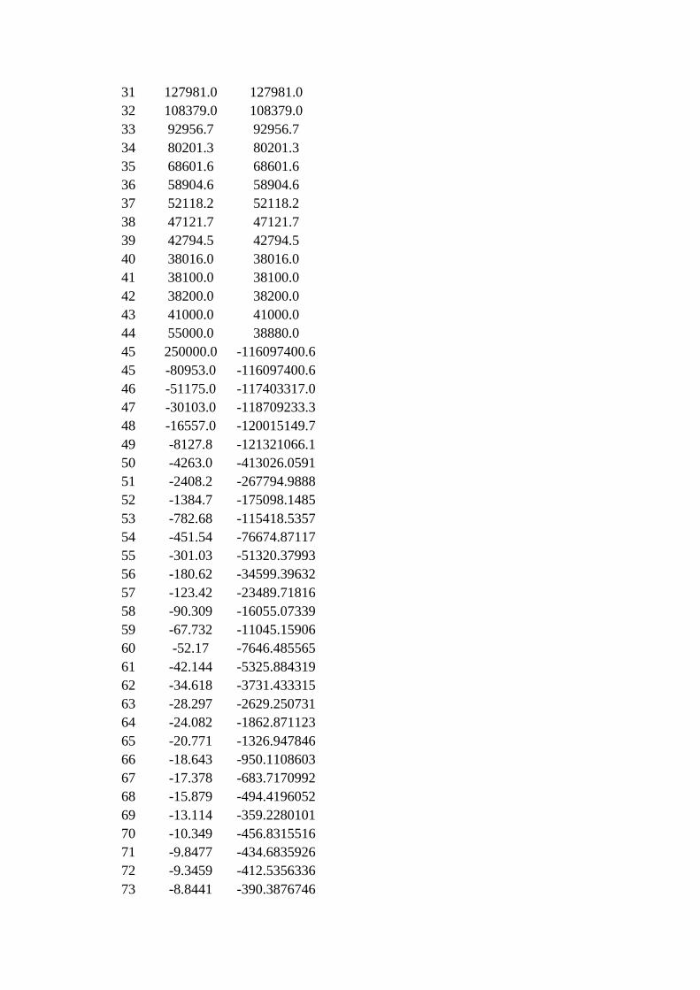
31 127981.0 127981.0

32 108379.0 108379.0

33 92956.7 92956.7

34 80201.3 80201.3

35 68601.6 68601.6

36 58904.6 58904.6

37 52118.2 52118.2

38 47121.7 47121.7

39 42794.5 42794.5

40 38016.0 38016.0

41 38100.0 38100.0

42 38200.0 38200.0

43 41000.0 41000.0

44 55000.0 38880.0

45 250000.0 -116097400.6

45 -80953.0 -116097400.6

46 -51175.0 -117403317.0

47 -30103.0 -118709233.3

48 -16557.0 -120015149.7

49 -8127.8 -121321066.1

50 -4263.0 -413026.0591

51 -2408.2 -267794.9888

52 -1384.7 -175098.1485

53 -782.68 -115418.5357

54 -451.54 -76674.87117

55 -301.03 -51320.37993

56 -180.62 -34599.39632

57 -123.42 -23489.71816

58 -90.309 -16055.07339

59 -67.732 -11045.15906

60 -52.17 -7646.485565

61 -42.144 -5325.884319

62 -34.618 -3731.433315

63 -28.297 -2629.250731

64 -24.082 -1862.871123

65 -20.771 -1326.947846

66 -18.643 -950.1108603

67 -17.378 -683.7170992

68 -15.879 -494.4196052

69 -13.114 -359.2280101

70 -10.349 -456.8315516

71 -9.8477 -434.6835926

72 -9.3459 -412.5356336

73 -8.8441 -390.3876746

74 -8.3424 -368.2397156

75 -7.8406 -346.0917566

76 -7.3389 -323.9437976

77 -6.8371 -301.7958386

78 -6.3354 -279.6478797

79 -5.8336 -257.4999207

80 -5.3318 -235.4051125

Annex 3 - Explanation of conservation equations

Continuity equation

A continuity equation is an equation that describes the transport of some quantity. The

majority of physical phenomena can be described using continuity equations, e.g., mass,

energy and momentum as they are conserved under their respective appropriate

conditions. The differential form of the continuity equation is Equation 13.

𝜕

𝜕𝑡𝜌 + 𝛻𝑗 = �̇� (13)

With:

ρ [kg/m³] Amount of quantity q per unit volume (density)

j Flux of q

�̇� Source or sink

Conservation of mass (medium: water with L. pneumophila)

In Fluid Dynamics, the mass conservation equation states that the rate at which mass

enters a system is the rate at which it leaves the system: 𝛻𝜌 · 𝑣 summed with the

accumulation of mass within the system: 𝜕

𝜕𝑡𝜌. The differential form of the mass

conservation equation is Equation 14.

𝜕

𝜕𝑡𝜌 + ∇𝜌 · �⃗� = 0 (14)

With:

ρ [kg/m³] Amount of quantity q per unit volume (density)

�⃗� [m/s] Velocity

Converting this equation to 1D gives Equation 15.

𝜕

𝜕𝑡𝜌 + 𝜌 ·

𝜕

𝜕𝑥𝑣𝑥 = 0 (15)

The integral form of this equation is Equation 16.

∭𝜕

𝜕𝑡𝜌 · 𝑑𝑉 = ∬

𝜕

𝜕𝑥𝑣𝑥 · 𝑑𝐴 (16)

Solving this integral gives Equation 17.

𝑉 ·𝑑𝜌

𝑑𝑡= 𝜌𝑖𝑛·𝑣𝑖𝑛 · 𝐴𝑖𝑛 − 𝜌𝑜𝑢𝑡 · 𝑣𝑜𝑢𝑡 · 𝐴𝑜𝑢𝑡 (17)

Conservation of energy (medium: water with L. pneumophila)

The law of conservation of energy states that energy can neither be created nor

destroyed. This law is combined with the First Law of Thermodynamics, which states

that, although energy cannot be created or destroyed, it can be transformed or

transferred from one form to another. This results in the energy conservation equation,

stating that the rate of change of energy inside the fluid element 𝜌 ·𝜕

𝜕𝑡𝑢, with 𝑢 = 𝐶 · 𝑇,

is the net flux of heat into the element (conduction component 𝜕

𝜕𝑥(𝑘 ·

𝜕𝑇

𝜕𝑥)) and transport

component 𝜌 · 𝑣𝑥 ·𝜕

𝜕𝑥𝑢 summed with the rate of working done on the element due to

body and surface forces �̇� + 𝛷. The differential form of the energy conservation

equation is Equation 18.

𝜕

𝜕𝑡𝜌 · 𝑢 + ∇𝜌 · 𝑣 · 𝑢⃗⃗ ⃗⃗ ⃗⃗ ⃗⃗ ⃗ = −∇𝑞𝑐 + �̇� + 𝛷 (18)

With:

𝑢 [J] Internal energy

𝑞𝑐 [W/m²] Conduction of heat, equal to ∇𝑘 · ∇𝑇

�̇� [W/m³] Heat source

𝛷 [W/m³] Heat losses due to friction and pressure losses

Converting this equation to 1D gives Equation 19.

𝜌 · (𝜕

𝜕𝑡𝑢 + 𝑣𝑥 ·

𝜕

𝜕𝑥𝑢) =

𝜕

𝜕𝑥(𝑘 ·

𝜕𝑇

𝜕𝑥) + �̇� + 𝛷 (19)

Modelica works with enthalpy in the heat flux equation 𝜌 · 𝑣𝑥 ·𝜕

𝜕𝑥𝑢. Knowing that the

enthalpy is ℎ = 𝑢 +𝑃

𝜌, if water is incompressible ℎ = 𝑐𝑝 · 𝑇.

The integral form of this equation becomes Equation 20.

∭𝜕

𝜕𝑡𝜌 · 𝑢 · 𝑑𝑉 = ∬

𝜕

𝜕𝑥𝑣𝑥 · ℎ · 𝑑𝐴 + ∬

𝜕

𝜕𝑥(𝑘 ·

𝜕𝑇

𝜕𝑥) · 𝑑𝐴 + ∭�̇� · 𝑑𝑉 + ∭𝛷 · 𝑑 (20)

Solving this integral gives Equation 21.

𝜌 · 𝑉 · (𝑑

𝑑𝑡𝑢) = 𝜌 · 𝑣𝑖𝑛 · 𝐴𝑖𝑛 · ℎ𝑖𝑛 + 𝜌 · 𝑣𝑜𝑢𝑡 · 𝐴𝑜𝑢𝑡 · ℎ𝑜𝑢𝑡 + 𝑄𝑐𝑜𝑛𝑑 + 𝑄𝑠𝑜𝑢𝑟𝑐𝑒 + 𝑄𝑑𝑖𝑠𝑠 (21)

Momentum conservation (medium: water with L. pneumophila)

The Momentum equation in Modelica is integrated in the form of the Navier-Stokes

equation, which results from Newton’s second law, stating that 𝐹 = 𝑚 · 𝑎. The Navier-

Stokes equation states that the mass, multiplied by the acceleration of fluid particles, is

proportional to the forces (volume forces and surface forces) acting on them. The

differential form of the momentum equation is Equation 22.

𝜕

𝜕𝑡𝜌 · 𝑣 + ∇𝜌 · 𝑣 · 𝑣⃗⃗ ⃗⃗ ⃗⃗ ⃗⃗ ⃗ = 𝜌 · 𝑔 − ∇𝑃 + 𝛻𝜏 (22)

Converting this equation to 1D gives Equation 23.

𝜌 · (𝜕

𝜕𝑡𝑣𝑥 + 𝑣𝑥 ·

𝜕

𝜕𝑥𝑣𝑥) = 𝜌 · 𝑔𝑥 −

𝜕𝑃

𝜕𝑥+ 𝛻(𝜇 · 𝛻𝑣𝑥) (23)

The integral form of this equation is Equation 24.

𝜕

𝜕𝑡∭�⃗� · 𝜌 · 𝑑𝑉 = ∬𝑣 · (𝜌(�⃗�) · 𝑑𝐴 + 𝜌 · 𝑔𝑥 −

𝜕𝑃

𝜕𝑥+ 𝛻(𝜇 · 𝛻𝑣𝑥)(24)

Solving this integral gives Equation 25.

𝜌 · 𝑉 ·𝑑�⃗⃗�

𝑑𝑡= 𝜌 · 𝑣𝑖𝑛

2 · 𝐴𝑖𝑛 − 𝜌 · 𝑣𝑜𝑢𝑡·2 𝐴𝑖𝑛 + 𝜌 · 𝑔𝑥 −

𝑑𝑃

𝑑𝑥+ ∇(𝜇 · ∇𝑣𝑥) (25)

This equation can be simplified to a pressure-based equation based on Bernoulli

(Equation 26).

0 =𝑣2

2

2𝑔−

𝑣12

2𝑔+ (ℎ2 − ℎ1) + (

𝑃2

𝜌𝑔−

𝑃1

𝜌𝑔) + (∆ℎ𝑓 + ∆ℎ𝑚 + ∆ℎ𝑝) (26)

With:

∆ℎ𝑝 Pressure rise by pump

∆ℎ𝑓 Major losses (in relation to length of pipe)

∆ℎ𝑚 Minor friction losses (e.g., fittings)

1 Entrance port

2 Exit port

Trace substance equation of L. pneumophila

The principle of the conservation equation for L. pneumophila concentration is based on

the principle of conservation of mass. Equation 2 and Equation 5 are coming from the

following equations. The differential form of the trace substance equation is Equation

27.

𝜕

𝜕𝑡𝐶 + ∇𝐶 · �⃗� = �̇� (27)

With:

𝐶 Total number of bacteria (cfu) per unit mixture volume (water with

bacteria)

�̇� Source and sink, this is the growth of L. pneumophila in water and the

mass transfer between water and biofilm

Converting this equation to 1D gives Equation 28.

𝜕

𝜕𝑡𝐶 +

𝜕

𝜕𝑥𝐶 · 𝑣𝑥 = �̇� (28)

The integral form of this equation is Equation 29.

∭𝜕

𝜕𝑡𝐶 · 𝑑𝑉 = ∬

𝜕

𝜕𝑥· 𝐶 · 𝑣𝑥 · 𝑑𝐴 + �̇� (29)

Solving this integral gives Equation 30.

𝑉 ·𝑑𝐶

𝑑𝑡= 𝐶𝑖𝑛 · 𝑣𝑖𝑛 · 𝐴𝑖𝑛 − 𝐶𝑜𝑢𝑡 · 𝑣𝑜𝑢𝑡 · 𝐴𝑜𝑢𝑡 + �̇� (30)

With: �̇� = 𝑉𝑝 · �̇�(𝑡) + 𝑘𝑐 · 𝐴𝑏 · (𝐶𝑏(𝑡) − 𝐶(𝑡)) in Equation 2.

Mass, momentum and energy conservation equation parameters to compare

different pipe and boiler models

Mass conservation: 𝜕

𝜕𝑡𝜌 + 𝜌 ·

𝜕

𝜕𝑥𝑣𝑥 = 0 (31)

Trace substances 𝜌

Can be solved by one node for the whole component, or the component can be split into

a number of nodes (nNodes).

Momentum conservation:∂

∂t𝑣𝑥 + 𝑣𝑥 ·

∂

∂x𝑣𝑥 = 𝜌 · 𝑔𝑥 −

𝜕𝑃

𝜕𝑥+ 𝛻(𝜇 · 𝛻𝑣𝑥) (32)

Gravity 𝜌 · 𝑔𝑥

Pressure drop 𝜕𝑃

𝜕𝑥

Laminar/turbulent flow 𝜕𝑃

𝜕𝑥 or 𝛻(𝜇 · 𝛻𝑣𝑥)

Friction/material roughness 𝛻(𝜇 · 𝛻𝑣𝑥)

Energy conservation: (𝜕

𝜕𝑡𝑢 + 𝑣𝑥 ·

𝜕

𝜕𝑥𝑢) =

𝜕

𝜕𝑥(𝑘 ·

𝜕𝑇

𝜕𝑥) + �̇� + 𝛷 (33)

Heat source �̇�

Heat exchange/insulation 𝜕

𝜕𝑥(𝑘 ·

𝜕𝑇

𝜕𝑥)

nNodes 𝜕

𝜕𝑥(𝑘 ·

𝜕𝑇

𝜕𝑥)

With:

𝑐𝑝 [J/kg·K] Heat capacity, used to calculate u

𝑔𝑥 [m/s²] Acceleration due to gravity

k [W/m·K] Thermal conductivity

P [Pa] Total pressure

�̇� [W/m³] Volumetric energy generation rate

t [s] Time

T [K] Absolute temperature

�⃗� [m/s] Mass-average velocity for multicomponent mixture (velocity

split up in vx, vy and vz)

μ [Pa·s] Viscosity

ρ [kg/m³] Mass density of mixture

𝛻 Partial derivative to x-, y- and z-direction, (𝜕

𝜕𝑥+

𝜕

𝜕𝑦+

𝜕

𝜕𝑧 )

Annex 4 - Pipe and boiler models: reasons for non-retention

Pipe models

Out of the comparison of the different pipe models in Table 2, there are four models

suitable for the authors’ applications.

Dynamic pipe: Dynamic pipe model with storage of mass and energy (Modelica

3.2.1)

Insulated pipe: Insulated pipe characterized by a UA value (OpenIDEAS 0.3.0)

Pipe insulated: Pipe with insulation, characterized by UA (OpenIDEAS 0.3.0)

Pipe: Pipe with finite volume discretization along flow path (Buildings 3.0.0)

‘Dynamic pipe’ model was not chosen for further development because insulation of the

pipe has not been taken into account in the standard model. ‘Insulated pipe’ and ‘Pipe

Insulated’, two very similar models, cannot be divided into smaller pipe volume

segments (nNodes). Moreover, material roughness, a parameter that is important to

simulate biofilm formation, is not taken into account. That is the reason why these

models were not retained.

Boiler models

‘Boiler’ and ‘OpenTank’ model were not chosen for further development because

insulation of the boiler has not been taken into account in the model. Although

insulation could easily be implemented if these models need to be used for this

application in future. Additionally these models and ‘Boiler polynomial’ cannot be

divided into smaller pipe volume segments (nNodes). In the ‘OpenTank’ and ‘Storage

Tank’ model the addition of a heat source is not possible. ‘StorageTank_OneIntHex’ is

not chosen because of the impossibility to add trace substance and the lack of pressure

drop and laminar/turbulent flow equations.

Annex 5 - Simulation model components used in pipe and boiler component

Table 11. Explanation of simulation model components used in the pipe and boiler

components.

Component Information

Generic fluid connector at design inlet for quasi one-dimensional fluid flow in a piping network

(incompressible or compressible, one or more phases, one or more substances)

Generic fluid connector at design outlet for quasi one-dimensional fluid flow in a piping network

(incompressible or compressible, one or more phases, one or more substances)

Collects the heat flows from m heatports to one single heatport

Fixed flow resistance with dp and m_flow as parameter

Connector used for 1-dimensional heat flow between components

HeatPort connector to be used for vectors of HeatPorts (vector dimensions must be added after dragging)

Lumped thermal element transporting heat without storing it

Mixing volume with inlet and outlet ports (flow reversal is allowed) with heat port

Heat exchanger typically submerged in a fluid with a second fluid circulating through it

Model to add buoyancy, if there is a temperature inversion in the tank

Model to reduce the numerical dissipation that is introduced by the standard first-order upwind discretization scheme, which is created when connecting fluid volumes in series

Ideal enthalphy mass flow rate sensor

Multiplexer block for three input connectors

Outputs the sum of the elements of the input vector

Output ‘Real' as connector

Conversion from theoretical continuity equation (Annex 3) to implementation of

equations in Modelica Buildings library

Mass and energy conservation equation

The conservation equations are implemented in Buildings Fluid Library under the

following form (Comparison of theoretical mass and energy equation and

implementation in Modelica.).

Table 12. Comparison of theoretical mass and energy equation and implementation in

Modelica.

Theoretical equation Implementation in Modelica

Mass conservation

equation of medium

(water containing

L. pneumophila and

nutrients)

𝑉 ·𝑑𝜌

𝑑𝑡= 𝜌𝑖𝑛 · 𝑣𝑖𝑛 · 𝐴𝑖𝑛 − 𝜌𝑜𝑢𝑡

· 𝑣𝑜𝑢𝑡 · 𝐴𝑜𝑢𝑡

der(m)=mb_flow

Mass conservation

equation of

L. pneumophila and

nutrients

𝑉 ·𝑑𝐶

𝑑𝑡= 𝐶𝑖𝑛 · 𝑣𝑖𝑛 · 𝐴𝑖𝑛

− 𝐶𝑜𝑢𝑡 · 𝑣𝑜𝑢𝑡

· 𝐴𝑜𝑢𝑡 + �̇�

der(mC)=mbC_flow+C_flow_internal

Energy conservation

equation of medium 𝜌 · 𝑉 · (

𝑑

𝑑𝑡𝑢) = 𝜌 · 𝑣𝑖𝑛 · 𝐴𝑖𝑛

· ℎ𝑖𝑛

+𝜌 · 𝑣𝑜𝑢𝑡 · 𝐴𝑜𝑢𝑡 · ℎ𝑜𝑢𝑡 + 𝑄𝑐𝑜𝑛𝑑

+ 𝛷

der(U)=Hb_flow+Q_flow

𝛷 = 0

In Buildings library, the mass and energy conservation equation can be found in the

MixingVolume model. In Figure A3.1, the Diagram view of the MixingVolume is

shown.

Figure A3.1 Diagram view of MixingVolume model.

In the Text view (Table 13), the following code can be found.

Table 13. Implementation of mass and energy conservation equation in Modelica. Model MixingVolume

extends Buildings.Fluid.MixingVolumes.BaseClasses.PartialMixingVolume MixingVolume

MixingVolume is an extension of PartialMixingVolume

Model PartialMixingVolume

extends Buildings.Fluid.Interfaces.LumpedVolumeDeclarations

“contains parameters and medium properties that are used in the lumped volume

model”

…

Buildings.Fluid.Interfaces.ConservationEquation steBal

(…)

if useSteadyStateTwoPort "Model for dynamic energy conservation"

…

Buildings.Fluid.Interfaces.ConservationEquation dynBal

(final simplify_mWat_flow = simplify_mWat_flow,

redeclare final package Medium = Medium,

final energyDynamics = energyDynamics,

final massDynamics = massDynamics,

final p_start = p_start,

final T_start = T_start,

final X_start = X_start,

final C_start = C_start,

final C_nominal = C_nominal,

final fluidVolume = V,

final initialize_p = Initialize_p,

m(start=V*rho_start),

nPorts=nPorts,

final mSenFac=mSenFac)

if not useSteadyStateTwoPort "Model for dynamic energy conservation"

PartialMixingVolume

This is a lumped volume model with the following properties: p, T, X, C. It contains

the whole mixture volume, in which the

number of trace substances is defined (i.e., L. pneumophila and nutrients).

The lumped volume model contains two

ways to solve the conservation Equations (steBal and dynBal). In our models,

dynBal, the model to solve the energy

conservation dynamically, has been chosen.

Model ConservationEquation "Lumped volume with mass and energy conservation"

…

Modelica.SIunits.Energy U(start=fluidVolume*rho_start*Medium.specificInternal

Energy(Medium.setState_pTX(

T=T_start,

p=p_start,

X=X_start[1:Medium.nXi])) +

(T_start - Medium.reference_T)*CSen, nominal = 1E5) "Internal energy of fluid";

ConservationEquation

The lumped volume works with T

(temperature), while the conservation equation works with u

(specificInternalEnergy). u is specified in

the Medium model. Therefore, a transition

to h (enthalpy) needs to happen. This is

equation

for i in 1:Medium.nC loop

mbC_flow[i] = sum(ports_mC_flow[:,i]);

end for;

mb_flow = sum(ports.m_flow);

Hb_flow = sum(ports_H_flow);

// Energy and mass conservation equations

if energyDynamics == Modelica.Fluid.Types.Dynamics.SteadyState then

0 = Hb_flow + Q_flow;

else der(U) = Hb_flow + Q_flow;

end if;

if massDynamics == Modelica.Fluid.Types.Dynamics.SteadyState then

0 = mb_flow + (if simplify_mWat_flow then 0 else mWat_flow_internal);

else der(m) = mb_flow + (if simplify_mWat_flow then 0 else mWat_flow_internal);

end if;

if substanceDynamics == Modelica.Fluid.Types.Dynamics.SteadyState then

zeros(Medium.nXi) = mbXi_flow + mWat_flow_internal * s;

else der(mXi) = mbXi_flow + mWat_flow_internal * s;

end if;

if traceDynamics == Modelica.Fluid.Types.Dynamics.SteadyState then

zeros(Medium.nC) = mbC_flow + C_flow_internal;

else der(mC) = mbC_flow + C_flow_internal;

end if;

added in the package Water of the Building

library, by using the function specificInternalEnergy (input T).

Energy conservation equation

Mass conservation equation of water

Mass conservation equation of L. pneumophila and nutrients. The value

for C_flow_internal is calculated in our

own developed components (part of our own DHW library), thus not belonging to

the Buildings library.

redeclare function extends specificInternalEnergy "Return specific internal energy"

extends Modelica.Icons.Function;

algorithm

// u := cv_const*(state.T - T0) - reference_p/d_const;

u := cv_const*(state.T - T0);

end specificInternalEnergy;

specificInternalEnergy

This function computes the specific internal energy of the fluid, but neglects the

(small) influence of the pressure term p/d.

package Water "Package with model for liquid water with constant density"

…

function enthalpyOfLiquid "Return the specific enthalpy of liquid"

extends Modelica.Icons.Function;

input Modelica.SIunits.Temperature T "Temperature";

output Modelica.SIunits.SpecificEnthalpy h "Specific enthalpy";

algorithm

h := cp_const*(T-reference_T);

end enthalpyOfLiquid;

Water

In package Water, the function

enthalpyOfLiquid is specified.

Momentum conservation

While the mass and energy conservation equations are written in the

PartialMixingVolume, the momentum conservation equation is written for each flow

element (e.g., pipe, boiler, pump) in the code of that specific component. The difference

is that the momentum equations take place

between two volume components, i.e., two mixing volumes. So, for a pipe model, the

total volume of the pipe is split into a predefined number of segments (an array

containing nNodes of MixingVolumes) along the flow path, thus containing nNodes

mass and energy conservation equations. Furthermore, only one equation is performed

to calculate the pressure drop for the whole (e.g., pipe) model, meaning the transfer of

momentum between the fluid and an adjacent surface is modelled using a lumped

approach (Table 14).

The momentum balance equation as specified in Annex 3 is Equation 34.

𝜌 · 𝑉 ·𝑑�⃗⃗�

𝑑𝑡= 𝜌 · 𝑣𝑖𝑛

2 · 𝐴𝑖𝑛 − 𝜌 · 𝑣𝑜𝑢𝑡2 · 𝐴𝑖𝑛 + 𝜌 · 𝑔𝑥 −

𝑑𝑃

𝑑𝑥+ ∇(𝜇 · ∇𝑣𝑥) (34)

In the Buildings library, a simplification is made by implementing a pressure-based

equation based on Bernoulli (Equation 35).

0 =𝑣2

2

2𝑔−

𝑣12

2𝑔+ (ℎ2 − ℎ1) + (

𝑃2

𝜌𝑔−

𝑃1

𝜌𝑔) + (∆ℎ𝑓 + ∆ℎ𝑚 + ∆ℎ𝑝) (35)

Table 14. Comparison of theoretical momentum equation and implementation in

Modelica.

Theoretical equation Implementation in Modelica

Momentum

conservation 0 =

𝑣22

2𝑔−

𝑣12

2𝑔+ (ℎ2 − ℎ1) + (

𝑃2

𝜌𝑔−

𝑃1

𝜌𝑔) +

(∆ℎ𝑓 + ∆ℎ𝑚 + ∆ℎ𝑝)

∆𝑝 = 𝜌 · 𝑔 · ∆ℎ𝑓

Assumptions:

𝑣1 = 𝑣2: Diameter of pipe is

constant

ℎ1 = ℎ2: Horizontal pipe

∆ℎ𝑝 = 0

∆ℎ𝑚 = ∆ℎ𝑓: Minor losses (e.g.,

fittings)

An example of the implementation of the momentum conservation in a pipe component

is given in Table 15. The principle of the used pipe model “Pipe_2_Leg”, is similar to

the Pipe model in Buildings library, except that it contains extra equations to calculate

the L. pneumophila concentration in water and biofilm.

Table 15. Implementation of momentum conservation equation in Modelica. Model Pipe_2_Leg "Pipe with finite volume discretization along flow path"

Extends DHW.LegionellaModels.Pipe_1_Leg(

diameter=sqrt(4*m_flow_nominal/rho_default/v_nominal/

Modelica.Constants.pi),

dp_nominal=2*dpStraightPipe_nominal,

preDro(dp(nominal=length*10)),

redeclare replaceable package Medium = DHW.LegionellaModels.WaterLeg,

vol(use_C_flow=true));

…

final parameter Modelica.SIunits.PressureDifference dpStraightPipe_nominal(displayU

nit="Pa")=Modelica.Fluid.Pipes.BaseClasses.WallFriction.Detailed.pressureLoss_m_fl

ow(

m_flow=m_flow_nominal,

rho_a=rho_default,

rho_b=rho_default,

mu_a=mu_default,

mu_b=mu_default,

length=length,

diameter=diameter,

roughness=roughness,

m_flow_small=m_flow_small)

"Pressure loss of a straight pipe at m_flow_nominal";

Pipe_2_Leg

Pipe model with roughness is an extension of a

pipe model without roughness (Pipe_1_Leg). A pressure drop is given to Pipe_1_Leg, that is

calculated as dpStraightPipe_nominal. This

pressure drop, taking into account the pressure losses of a straight pipe, is multiplied by two to

incorporate the minor losses ∆ℎ𝑚.

The total pressure drop, dp_nominal, is

calculated in Pipe_2_Leg with the function pressureLoss_m_flow based on the material

roughness.

In case the velocity is not the nominal velocity,

this pressure drop is adapted by the model

preDro, which is available in Pipe_1_Leg.

model Pipe_1_Leg "Model of a pipe with finite volume discretization along the

flow path"

extends Modelica.Icons.Example;

extends Buildings.Fluid.Interfaces.LumpedVolumeDeclarations;

extends Buildings.Fluid.Interfaces.PartialTwoPortInterface(final show_T=true);

extends Buildings.Fluid.Interfaces.TwoPortFlowResistanceParameters(final

Pipe_1_Leg

LumpedVolumeDeclarations is a record that

contains the parameters and medium properties that are used in the lumped volume model.

TwoPortFlowResistanceParameters is a record

computeFlowResistance=(abs(dp_nominal) > Modelica.Constants.eps));

Buildings.Fluid.FixedResistances.PressureDrop preDro(…);

Buildings.Fluid.MixingVolumes.MixingVolume [nSeg] vol(…)

that contains parameters that are used to compute

the pressure drop in models that have one fluid stream. Furthermore the pipe model contains an

array of MixingVolumes and a model that

calculates the pressure drop.

preDro to relate dp_nominal to m, in case m is not

m_nominal. MixingVolume to calculate mass and energy conservation equations.

Function pressureLoss_m_flow

Re := diameter*abs(m_flow)/(crossArea*mu);

lambda2 := if Re <= Re1 then 64*Re else

(if Re >= Re2 then 0.25*(Re/Math.log10(Delta/3.7 + 5.74/Re^0.9))^2

Else interpolateInRegion2(Re, Re1, Re2, Delta));

dp :=length*mu*mu/(2*rho*diameter*diameter*diameter)*

(if m_flow >= 0 then lambda2 else -lambda2);

pressureLoss_m_flow

To calculate the pressure drop associated with

frictional effects (∆ℎ𝑓),the Darcy-Weisbach

equation is applied, stating that ∆𝑝 = 𝜁 ·𝐿

𝐷·𝜌·𝑣2

2.

The pressure drop due to wall friction is computed

as product of dynamic pressure and a loss factor

𝜁. The loss factor 𝜁is based on the Colebrook-

White equation, this equation is translated in Modelica in the function pressureLoss_m_flow. A

problem arises because the Colebrook-White

equation is an iterative formula. To solve this, an explicit variation of the Colebrook-White

equation is used, namely the Swamee-Jain

equation, for flow in a completely filled pipe with circular section.

Annex 6 - Understanding the simulation log basics

When you run a simulation in Dymola, a simulation log is generated. The statistics

listed in Table 16 can be considered the key performance indicators of the simulation

computational performance.

Table 16. Key performance indicators of the simulation computational performance

(Claytex 2016)

Simulation log variable General definition of variable

CPU-time for integration

CPU-time for one GRID

interval

Number of result points

Number of GRID points

Number of (successful)

steps

Number of F-evaluations

Number of H-evaluations

Number of Jacobian-

evaluations

Number of (model) time

events

Number of (U) time events

Number of state events

The total CPU-time of the simulation.

The CPU-time to calculate one grid interval.

The total number of simulation steps stored by Dymola in the result

file

Evenly spaced points with spacing determined from “Interval

length” or “number of intervals” and the simulation time.

Total number of simulation steps calculated by the solver. The

result points are extrapolated from these steps.

Number of times equations used to calculate the gradient of the

states were run.

Number of times the crossing functions had to be calculated. These

functions are used to determine when an event occurs.

The Jacobian is utilised by the solver method during the solving

process. The solver method requests that the Jacobian be updated

throughout the simulation.

Events that are generated at a given time.

Events that are generated when discrete input signal changes occur.

Minimum integration

stepsize

Maximum integration

stepsize

Maximum integration

order

A real elementary relation changes its value, for example “x>2”

changes its value.

Minimum stepsize used during simulation.

Maximum stepsize used during simulation.

The maximum integration order used by the solver.