Embed Size (px)
Citation preview

Simulation of Ground-Water Discharge toBiscayne Bay, Southeastern Florida
Water-Resources Investigations Report 00-4251
U.S. DEPARTMENT OF THE INTERIORU.S. GEOLOGICAL SURVEY
Prepared as part of theU.S. GEOLOGICAL SURVEY PLACE-BASED STUDIES PROGRAMand in cooperation with theU.S. ARMY CORPS OF ENGINEERS
BiscayneBay
Municipalwell field
Evapotranspiration
Surface waterin Everglades
Recharge
Lateralboundaryflow
Brackish water
Freshwater
Seawater
Submarineground-water
discharge
BISCAYNEAQUIFER
Canal Canal
Water table Water table
Rainfall
Municipalwell field

Simulation of Ground-Water Discharge toBiscayne Bay, Southeastern Florida
Prepared as part of theU.S. GEOLOGICAL SURVEY Place-Based Studies Programand in cooperation with theU.S. ARMY CORPS OF ENGINEERS
By Christian D. Langevin
Tallahassee, Florida2001
U.S. GEOLOGICAL SURVEY
Water-Resources Investigations Report 00-4251

Copies of this report can be purchased from:
U.S. Geological SurveyBranch of Information ServicesBox 25286Denver, CO 80225-0286888-ASK-USGS
Use of trade, product, or firm names in this publication is for descriptive purposes only and does not imply endorsement by the U.S. Geological Survey.
For additional informationwrite to:
District ChiefU.S. Geological SurveySuite 3015227 N. Bronough StreetTallahassee, FL 32301
Additional information about water resources in Florida is available on the World Wide Web at http://fl.water.usgs.gov
U.S. DEPARTMENT OF THE INTERIORGALE A. NORTON, Secretary
U.S. GEOLOGICAL SURVEYCHARLES G. GROAT, Director

Contents III
CONTENTS
Abstract.................................................................................................................................................................................. 1Introduction ........................................................................................................................................................................... 2
Purpose and Scope ....................................................................................................................................................... 2Methods of Field Investigation.................................................................................................................................... 2Previous Studies........................................................................................................................................................... 5Acknowledgments ....................................................................................................................................................... 6
Hydrogeology of Southeastern Florida.................................................................................................................................. 6Hydrostratigraphy ........................................................................................................................................................ 7Aquifer Properties........................................................................................................................................................ 8Water-Budget Components.......................................................................................................................................... 10
Rainfall, Evapotranspiration, and Runoff .......................................................................................................... 10Surface-Water/Ground-Water Interaction ......................................................................................................... 10Ground-Water Withdrawals............................................................................................................................... 13
Freshwater-Saltwater Transition Zone......................................................................................................................... 14Simulation of Ground-Water Discharge to Biscayne Bay..................................................................................................... 22
Governing Equations ................................................................................................................................................... 24SEAWAT Simulation Code.......................................................................................................................................... 26Cross-Sectional Ground-Water Flow Models.............................................................................................................. 27
Model Design..................................................................................................................................................... 27Model Calibration and Simulation Results ........................................................................................................ 29Sensitivity Analysis ........................................................................................................................................... 33
Regional-Scale Ground-Water Flow Model ................................................................................................................ 34Spatial and Temporal Discretization.................................................................................................................. 35Assignment of Aquifer Parameters.................................................................................................................... 35Boundary Conditions ......................................................................................................................................... 38
Biscayne Bay............................................................................................................................................ 38Inland Model Domain Boundaries........................................................................................................... 38Lower Model Boundary ........................................................................................................................... 39
Internal Hydrologic Stresses .............................................................................................................................. 39Canals....................................................................................................................................................... 39Ponded Surface Water.............................................................................................................................. 40Recharge and Runoff ............................................................................................................................... 40Evapotranspiration ................................................................................................................................... 40Municipal Well Fields.............................................................................................................................. 42
Initial Conditions ............................................................................................................................................... 42Calibration Procedure and Model Results ......................................................................................................... 42
Comparison of Simulated and Observed Heads ...................................................................................... 42Comparison of Simulated and Observed Canal Baseflow....................................................................... 43Net Recharge............................................................................................................................................ 51Saltwater Interface ................................................................................................................................... 51Ground-Water Flow to Biscayne Bay...................................................................................................... 54
Sensitivity Analysis ........................................................................................................................................... 56Model Limitations ....................................................................................................................................................... 59
Conclusions ........................................................................................................................................................................... 60References Cited.................................................................................................................................................................... 61Appendix I: Lithologic Descriptions of Selected Cores as Determined for this Study ......................................................... 67Appendix II: Field Data Collected as Part of this Study ....................................................................................................... 85Appendix III: Monitoring Stations Used in this Study .......................................................................................................... 101Appendix IV: Verification of the SEAWAT Code ................................................................................................................. 121

IV Contents
PLATES1. Sections showing sensitivity analysis results for the Coconut Grove model.................................................. pocket2. Sections showing sensitivity analysis results for the Deering Estate model................................................... pocket3. Maps showing boundary conditions, internal hydrologic stresses, and hydraulic conductivity
zonation of the regional-scale model .............................................................................................................. pocket
FIGURES1-2. Maps showing:
1. Location of study area, domain of regional-scale model, and location of field transects .............................. 32. Natural physiographic features of southern Florida ....................................................................................... 7
3. Hydrogeologic section showing relations of geologic formations, aquifers, and semipermeable units of thesurficial aquifer system across central Miami-Dade County .................................................................................. 8
4-5. Maps showing:4. Water-table elevation for May 1993, Miami-Dade County, Florida .............................................................. 115. Water-table elevation for November 1993, Miami-Dade County, Florida ..................................................... 12
6-10. Graphs showing:6. Totals of annual and monthly rainfall, 1989-98 ............................................................................................. 137. Municipal well-field withdrawals from the Biscayne aquifer in Miami-Dade County from
January 1989 to September 1998 ................................................................................................................... 148. Lines of equal chloride concentration and results from a flow-net analysis for the
Cutler Ridge area, September 18, 1958.......................................................................................................... 159. Lines of equal chloride concentration for the Silver Bluff area, November 2, 1954 ..................................... 1610. Lines of equal chloride concentration from March 1998 to February 1999 for
the Coconut Grove, Deering Estate, and Mowry Canal transects .................................................................. 1911-12. Maps showing:
11. Location of saltwater intrusion lines in southern Florida based on previous studies, the Ghyben-Herzberg relation, and a geophysical survey. ................................................................................... 20
12. Ground-water monitoring wells in the Biscayne aquifer used to monitor the location of thesaltwater intrusion line in Miami-Dade County ............................................................................................. 21
13-14. Graphs showing:13. Chloride concentrations relative to time for selected monitoring wells in Miami-Dade County................... 2214. Stage fluctuations in Biscayne Bay, Florida, 1989-99, plotted as average daily and monthly
averages and hourly values............................................................................................................................. 2315. Three-dimensional diagram showing conceptual hydrologic model used to develop numerical
models of groundñwater flow ................................................................................................................................. 2416. Map showing location of the two-dimensional, cross-sectional models for Coconut Grove and Deering Estate .. 2817. Grids showing boundary conditions and finite-difference grid for the Coconut Grove and Deering
Estate models........................................................................................................................................................... 3018. Cross sections showing calibration results for the Coconut Grove and Deering Estate models............................. 32
19-20. Graphs showing:19. Simulated ground-water discharge to Biscayne Bay for the Deering Estate model....................................... 3320. Simulated water budget for the Coconut Grove and Deering Estate models ................................................. 34
21-24 Maps showing:21. Finite-difference grid for the regional-scale ground-water flow model in southern Florida.......................... 3622. Land-surface elevation of southern Florida used in the regional-scale ground-water flow model ................ 3723. Land use of southern Florida for 1995 ........................................................................................................... 4124. Location of ground-water monitoring wells in southern Florida used to calibrate the regional-scale
ground-water flow model and average differences between observed and simulated values of head ........... 4425-26. Graphs showing:
25. Comparison between observed and simulated monthly average heads for selected monitoring wells near the coast......................................................................................................................................... 45
26. Calibration statistics for errors between observed heads and heads simulated by the regional-scale ground-water flow model ............................................................................................................................... 47

Contents V
27. Map showing location of surface-water basins in southern Florida and the mean absolute error between observed and simulated canal baseflow .................................................................................................................. 48
28. Graphs showing comparison between observed and simulated values of monthly average canal baseflow for selected surface-water basins............................................................................................................................. 49
29-30. Maps showing:29. Simulated values of average annual net recharge from the regional-scale ground-water flow model
for 1989-98 ..................................................................................................................................................... 5230. Simulated values of ground-water salinity at the base of the Biscayne aquifer compared with the
1995 saltwater intrusion line .......................................................................................................................... 5331. Graphs showing:
31. Total salt mass in the Biscayne aquifer as simulated by the regional-scale ground-water flow model...................................................................................................................................................... 54
32. Simulated fresh ground-water discharge to Biscayne Bay............................................................................. 5533. Simulated fresh ground-water discharge compared with measured surface-water discharge
to Biscayne Bay.............................................................................................................................................. 5634. Graphs showing sensitivity analysis of regional-scale model depicting range of simulated fresh
ground-water discharge to Biscayne Bay ....................................................................................................... 58A1. Schematic showing boundary conditions and model parameters for the Henry problem....................................... 123A2. Graphs showing comparison between SEAWAT and SUTRA for the Henry problem........................................... 124A3. Schematic showing boundary conditions and model parameters for the Elder problem ........................................ 125A4. Schematics showing comparison between SEAWAT, SUTRA, and Elderís solution for the Elder problem ......... 126A5. Schematic showing boundary conditions and model parameters for the HYDROCOIN problem......................... 127A6. Graph showing comparison between SEAWAT and MOCDENSE for the HYDROCOIN problem ..................... 127
TABLES1. Properties of ground-water monitoring wells installed for this study ................................................................... 42. Field data used to construct cross sections of chloride concentration and calibrate cross-sectional models ......... 173. Results from the time-domain electromagnetic (TDEM) soundings near Mowry Canal....................................... 184. Aquifer parameters and boundary stresses used in the calibrated cross-sectional models..................................... 315. Runoff coefficients and evapotranspiration extinction depths for different land-use categories ........................... 40
EQUATIONS1. Hydraulic conductivity as a function of permeability and fluid properties ............................................................ 92. Variable-density form of ground-water flow equation ........................................................................................... 253. Solute-transport equation........................................................................................................................................ 254. Variable density form of Darcyís law ..................................................................................................................... 255. Darcyís law for horizontal ground-water flow in terms of pressure....................................................................... 256. Darcyís law for vertical ground-water flow in terms of pressure........................................................................... 257. Mathematical expression for head .......................................................................................................................... 258. Relation between freshwater head, actual head, and elevation .............................................................................. 269. Relation between freshwater head, elevation, and pressure ................................................................................... 2610. Darcyís law for horizontal ground-water flow in terms of freshwater head........................................................... 2611. Darcyís law for vertical ground-water flow in terms of freshwater head............................................................... 2612. Variable-density ground-water flow equation as a function of freshwater head .................................................... 26

VI Contents
Sea level: In this report, ì sea levelî refers to the National Geodetic Vertical Datum of 1929--a geodetic datum derived from a general adjustment of the first-order level nets of both the United States and Canada, formerly called Sea Level Datum of 1929.
Conversion Factors, Abbreviations, and Datum
Multiply By To obtain
centimeter 0.3937 inchcentimeter per year 0.3937 inch per year
meter 3.2808 footmeter per day 3.2808 foot per daysquare meter 10.7636 square foot
square meter per day 10.7636 square foot per daycubic meter 35.3134 cubic foot
cubic meter per day 35.3134 cubic foot per daycubic meter per day 4.0872 x 10⁻⁴ cubic foot per secondcubic meter per day 264.2 gallon per day
kilometer 0.6214 milekilogram 2.2046 pound
kilogram per cubic meter 0.0624 pound per cubic foot
Abbreviations used for dimensions
M Mass
L Length
T Time

Abstract 1
Simulation of Ground-Water Discharge to Biscayne Bay, Southeastern FloridaBy Christian D. Langevin
Abstract
As part of the Place-Based Studies Program, the U.S. Geological Survey initiated a project in 1996, in cooperation with the U.S. Army Corps of Engineers, to quantify the rates and patterns of submarine ground-water discharge to Biscayne Bay. Project objectives were achieved through field investigations at three sites (Coconut Grove, Deering Estate, and Mowry Canal) along the coastline of Biscayne Bay and through the development and calibration of variable-density, ground-water flow models. Two-dimensional, vertical cross-sectional models were developed for steady-state conditions for the Coconut Grove and Deering Estate transects to quantify local-scale ground-water discharge patterns to Biscayne Bay. A larger regional-scale model was developed in three dimensions to sim-ulate submarine ground-water discharge to the entire bay. The SEAWAT code, which is a com-bined version of MODFLOW and MT3D, was used to simulate the complex variable-density flow patterns.
Field data suggest that ground-water dis-charge to Biscayne Bay relative to the shoreline is restricted to within 300 meters at Coconut Grove, 600 to 1,000 meters at Deering Estate, and 100 meters at Mowry Canal. The vertical cross-sectional models, which were calibrated to the field data using the assumption of steady state, tend to focus ground-water discharge to within 50 to 200 meters of the shoreline. With homogeneous distributions for aquifer parameters and a con-stant-concentration boundary for Biscayne Bay,
the numerical models could not reproduce the lower ground-water salinities observed beneath the bay, which suggests that further research may be necessary to improve the accuracy of the numerical simulations. Results from the cross-sectional models, which were able to simulate the approximate position of the saltwater interface, suggest that longitudinal dispersivity ranges between 1 and 10 meters, and transverse disper-sivity ranges from 0.1 to 1 meter for the Biscayne aquifer.
The three-dimensional, regional-scale model was calibrated to ground-water heads, canal baseflow, and the general position of the saltwater interface for nearly a 10-year period from 1989 to 1998. The mean absolute error between observed and simulated head values is 0.15 meter. The mean absolute error between observed and simulated baseflow is 3 x 10⁵ cubic meters per day. The position of the simulated saltwater interface generally matches the position observed in the field, except for areas north of the Miami Canal where the simulated saltwater inter-face is located about 5 kilometers inland of the observed saltwater interface. Results from the regional-scale model suggest that the average rate of fresh ground-water discharge to Biscayne Bay for the 10-year period (1989-98) is about 2 x 10⁵ cubic meters per day for 100 kilometers of coastline. This simulated discharge rate is about 6 percent of the measured surface-water discharge to Biscayne Bay for the same period. The model also suggests that nearly 100 percent of the fresh ground-water discharge is to the northern half of Biscayne Bay, north of the Cutler Drain Canal.

2 Simulation of Ground-Water Discharge to Biscayne Bay, Southeastern Florida
South of the Cutler Drain Canal, coastal lowlands prevent the water table from rising high enough to drive measurable quantities of ground water to Biscayne Bay. Annual variations in sea-level elevation, which can be as large as 0.3 meter, have a substantial effect on rates of ground-water discharge. During 1989-98, simulated rates of ground-water discharge to Biscayne Bay gener-ally are highest when sea level is relatively low.
INTRODUCTION
Biscayne Bay is a coastal barrier-island lagoon that relies on substantial quantities of freshwater to sustain its estuarine ecosystem. During the past cen-tury, field observations suggest that the mechanism for the delivery of freshwater to Biscayne Bay has changed from a system largely controlled by wide-spread and continuous submarine discharge and over-land sheetflow to one controlled by episodic releases of surface water at the mouths of canals. Current ecosystem restoration efforts in southern Florida are examining alternative water-management scenarios that could further change the quantity and timing of freshwater delivery to the bay. There is concern that these proposed modifications could adversely affect bay salinities.
To evaluate the effects of the modifications on Biscayne Bay, the U.S. Army Corps of Engineers (USACE) is constructing a surface-water hydrody-namic circulation model. To achieve a reasonable cali-bration, this model requires the accurate specification of freshwater discharges to the bay. The two most important mechanisms for freshwater discharge to Biscayne Bay are thought to be canal discharges and submarine ground-water discharge from the Biscayne aquifer. Canal discharges are routinely measured and recorded, but few studies have attempted to quantify the rates and patterns of submarine ground-water dis-charge. Depending on the method, estimates of subma-rine ground-water discharge can range over several orders of magnitude.
As part of the Place-Based Studies program, the U.S. Geological Survey (USGS), in cooperation with the USACE, initiated a project in 1996 to quantify the rates and patterns of submarine ground-water dis-charge to Biscayne Bay. This was accomplished through field investigation and ground-water flow
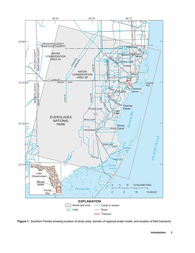
simulation at three sites along the coastline of Biscayne Bay and development of a numerical ground-water flow model that covers most of Miami-Dade County and parts of Broward and Monroe Coun-ties (fig. 1). Study results have been incorporated into the hydrodynamic circulation model under develop-ment by the USACE.
Purpose and Scope
The purposes of this report are to: (1) document the development of a regional-scale, three-dimen-sional numerical model that simulates variable-density ground-water discharge to Biscayne Bay, and (2) present an estimate of submarine ground-water discharge to Biscayne Bay. To properly simulate ground-water flow, processes affecting ground-water flow were characterized and represented mathemati-cally. Two local-scale models were developed in cross section to simulate the complex ground-water dis-charge patterns near the coast of Biscayne Bay. Ground-water data collected for this study from March 1997 to February 1998 are presented and used with an assumption of steady-state conditions to calibrate the cross-sectional models. Results from the cross-sectional models were used to aid development of the regional-scale model that simulates transient ground-water discharge in three dimensions. The regional-scale model was calibrated with field data from 1989 through 1998 to ensure it is a reasonable representa-tion of the physical system.
Methods of Field Investigation
A field investigation was conducted to collect data that would help quantify ground-water discharge to Biscayne Bay. The design of the field investigation was based on the general and widely accepted concept that fresh ground water flowing toward a coastal boundary will flow up and over a saltwater wedge. To better characterize this flow pattern within the study area, three transects, each located on a ground-water flow line toward Biscayne Bay, were selected for fur-ther study. The locations of these transects, referred to as Coconut Grove, Deering Estate, and Mowry Canal, are shown in figure 1.
Introduction 3
27
826
95
836
1
1
874
1
997
1
41
Studyarea
LakeOkeechobee
FloridaBay
AT
LA
NT
ICO
CE
AN
Bis
cayn
eB
ay
������
������
������
�����
����� ����� �����
Florida Bay
CoconutGrove
DeeringEstate
MowryCanal
EVERGLADESNATIONAL
PARK
CO
LLIE
RC
OU
NT
Y
MIA
MI-
DA
DE
CO
UN
TY
0 15 MILES5 10
0 15 KILOMETERS5 10
EXPLANATION
BROWARD COUNTY
MIAMI-DADE COUNTY
MO
NR
OE
CO
UN
TY
Homestead
Tamiami Canal
SnapperCreek Canal
Mowry Canal
Canal 111
Canal
Canal
Canal
Cre
ek
Bla
ck
Model Land
CutlerRidge
Princeton
DrainCanal
Cutler
FLO
RID
A’S
TU
RN
PIK
E
Leve
e67
ALe
vee
67C
Levee
67
WATERCONSERVATION
AREA 3A
WATERCONSERVATION
AREA 3BLevee 29
Levee
30
Levee
31N
NorthMiami
Snake Creek
Biscayne Canal
Little River Canal
Hialeah
Miam
i Canal
Miami
SilverBluff
VirginiaKey
BarnesSound
Car
dSo
und
FLO
RID
A’S
TU
RN
PIK
E
C
or
l
al bGa len
sC
a
a
MIA
MI-
DA
DE
CO
UN
TY
Canal
Model grid area
Lake
Canal or stream
Road
Transect
Figure 1. Southern Florida showing location of study area, domain of regional-scale model, and location of field transects.

4 Simulation of Ground-Water Discharge to Biscayne Bay, Southeastern Florida
The field investigation was initiated by installing ground-water monitoring wells at each of the three transects. In an effort to fully charac-terize the transition zone between fresh and saline ground water, monitoring wells were installed both inland and offshore. Inland monitoring wells were installed by the Florida Geological Survey, and the
offshore monitoring wells were installed by the USGS. The offshore wells were installed from a floating barge using the methods presented in Shinn and others (1994). Coordinates, screened intervals, and other specifications for these and other monitoring wells installed for this study are given in table 1.
Table 1. Properties of ground-water monitoring wells installed for this study [N/A, not available]
Wellidentification Latitude Longitude
Total depth
(meters)
Depth to screen(meters)
Casing eleva-tion
(meters)Top Bottom
Coconut Grove transect
G-3654 25°43′22″ 80°14′32″ 7.0 4.6 6.1 -0.99G-3655 25°43′22″ 80°14′32″ 3.0 1.5 3.0 N/AG-3656 25°43′14″ 80°14′26″ 10.7 9.1 10.7 -1.56G-3657 25°43′14″ 80°14′26″ 3.0 1.5 3.0 -1.54G-3658 25°43′09″ 80°14′19″ 7.6 6.1 7.6 N/AG-3659 25°43′09″ 80°14′19″ 3.0 1.5 3.0 -1.42G-3747 25°43′27″ 80°14′52″ 30.8 28.4 29.9 4.90G-3748 25°43′32″ 80°14′15″ 10.8 9.3 10.8 .72G-3749 25°43′32″ 80°14′15″ 19.3 17.9 19.3 .74G-3750 25°43′32″ 80°14′15″ 30.8 28.4 30.0 .69
Deering Estate transect
G-3646 25°36′52″ 80°18′20″ 8.5 7.0 8.5 N/AG-3647 25°36′52″ 80°18′20″ 2.4 .9 2.4 N/AG-3648 25°36′48″ 80°18′12″ 6.1 4.6 6.1 N/AG-3649 25°36′48″ 80°18′12″ 3.0 1.5 3.0 N/AG-3650 25°36′46″ 80°18′05″ 6.1 4.6 6.1 N/AG-3651 25°36′46″ 80°18′05″ 3.0 1.5 3.0 N/AG-3652 25°36′40″ 80°17′49″ 6.1 4.6 6.1 N/AG-3653 25°36′40″ 80°17′49″ 2.4 .9 1.5 N/AG-3751 25°36′50″ 80°18′25″ 3.3 1.8 3.3 .67G-3752 25°36′50″ 80°18′25″ 16.2 14.7 16.2 .71G-3753 25°36′50″ 80°18′25″ 30.8 27.0 28.6 .73G-3754 25°36′50″ 80°18′25″ 7.4 5.9 7.4 .75G-3755 25°36′58″ 80°18′35″ 30.8 28.3 29.8 3.38
Mowry Canal transect
G-3629 25°28′26″ 80°20′24″ 13.1 10.0 11.5 N/AG-3630 25°28′26″ 80°20′24″ 2.7 1.2 2.7 N/AG-3631 25°28′28″ 80°20′15″ 6.1 4.6 6.1 N/AG-3632 25°28′28″ 80°20′15″ 3.4 1.8 3.4 N/AG-3633 25°28′28″ 80°20′15″ 1.2 .5 1.2 N/AG-3634 25°28′29″ 80°20′07″ 6.1 4.6 6.1 N/AG-3635 25°28′29″ 80°20′07″ 3.4 1.8 3.4 N/AG-3636 25°28′29″ 80°19′59″ 6.1 4.6 6.1 N/AG-3637 25°28′29″ 80°19′59″ 3.4 1.8 3.4 N/AG-3638 25°28′23″ 80°20′25″ 6.1 4.6 6.1 N/AG-3639 25°28′23″ 80°20′25″ 2.4 .9 2.4 N/AG-3756 25°28′13″ 80°20′47″ 30.6 26.8 28.3 1.62G-3757 25°28′13″ 80°20′48″ 20.0 18.5 20.0 1.76G-3758 25°28′13″ 80°20′48″ 9.4 7.8 9.4 1.66G-3759 25°28′25″ 80°22′13″ 30.8 27.6 29.1 1.04

Introduction 5
During the installation of selected monitoring wells, lithologic cores were collected and analyzed to provide a better understanding of the stratigraphy and hydrogeologic characteristics at the monitoring well locations (app. I). Permeameter analyses were per-formed on several rock samples extracted from the cores, but the analyses were inconclusive. For selected inland monitoring wells, geophysical logging was performed by the South Florida Water Management District prior to setting the steel surface casing.
Water samples were collected with a centrifugal pump from selected monitoring wells for each month from March 1998 to February 1999. Measurements of depth to water were recorded prior to sampling, and if the well had been leveled, a water-table elevation was calculated. During the first 3 months, water samples were analyzed by the USGS for chloride concentra-tion, [Cl-], using the titration method (Brown and oth-ers, 1974). Measurements of specific conductance (SC) also were performed on the ground-water sam-ples. These data are included in appendix II. After 3 months of directly measuring chloride concentra-tions, it was determined that chloride concentrations could be adequately estimated from measurements of specific conductance, which are easier to perform. Chloride concentrations for all subsequent ground-water samples were estimated from specific conduc-tance using the following equation:
,
where [Cl-] is in milligrams per liter and SC is in microsiemens per centimeter. This polynomial equa-tion was created by a fit to 120 measurements of specific conductance and chloride concentrations and represents the data with a correlation coefficient (R2) of 0.9967.
The numerical model used in this study requires concentrations of total dissolved solids (TDS) rather than chloride concentrations. Chloride concentrations were linearly converted to TDS by assuming that sea-water has a chloride concentration of 19,800 mg/L (milligrams per liter) and a TDS value of 35,000 mg/L (Parker, and others, 1955). Fish (1988) estimates that water-rock interactions in the surficial aquifer of southeastern Florida can affect the TDS value by 350 to 550 mg/L; therefore, the TDS values in this study, which were estimated from chloride concentrations, may contain a 1 to 2 percent error relative to the
observed range of TDS values. This suggests that a linear relation between chloride and TDS is reason-able, even for ground-water samples.
During the initial part of the field investigation, much time was spent trying to obtain reliable results from seepage meters. A seepage meter is a cylindrical tube that is pressed into the bottom sediments of a surface-water body; seepage rates are determined by measuring liquid volumes in a bag attached to the tube. After many unsuccessful attempts, it was determined that seepage meters could not be used within the tidal environment of Biscayne Bay because flow rates mea-sured at seepage meters were not in agreement with tidal phase, or were not proportional to vertical head differences at nested offshore monitoring wells. There is evidence that seepage meters may not work in tidal environments or under certain conditions because they may be artificially pumped from tides, waves, and fluctuations in barometric pressure (C. Reich, U.S. Geological Survey, oral commun., 2000). This artificial pumping can result in seepage measurements that are not representative of the actual seepage rate.
To better delineate the position of the saltwater interface, time-domain electromagnetic (TDEM) soundings were made at the Mowry Canal transect. The TDEM method has been successfully used in southern Florida to locate the saltwater interface (Son-enshein, 1997; Fitterman and others, 1999; and Hittle, 1999) and lithologic boundaries (Shoemaker, 1998). The TEMIX software (Interpex Limited, 1996) was used to invert the geophysical data. The approach described by Fitterman and others (1999) was used to interpret the inverted TDEM data and determine approximate depths of the saltwater interface.
Previous Studies
Taniguchi and others (1999) compiled rates of submarine ground-water discharge from around the world. He concludes that most measured seepage rates are less than 0.1 m/d (meter per day), a rate that includes recirculated seawater. Byrne (1999) used seepage meters and a form of Darcyís law to estimate ground-water discharge to Biscayne Bay. He found that most of the ground-water discharge occurred within the first 400 m (meters) of shore. His estimates of submarine ground-water discharge range from 10 to 20 m3/d (cubic meters per day) per meter of shoreline. Assuming that ground-water discharge occurs only within the first 400 m from shore, Byrneís (1999)
Clñ[ ] 1 10 6ñ SC2 0.3224 SC 177.7ñ⋅+⋅ ⋅=

6 Simulation of Ground-Water Discharge to Biscayne Bay, Southeastern Florida
average discharge estimates range from 0.025 to 0.050 m/d, similar to the average rate compiled by Taniguchi and others (1999). Byrneís (1999) estimates of total ground-water discharge also include the vol-ume of recirculated seawater.
From the 1940ís to the 1960ís, many studies on the Biscayne aquifer and in particular saltwater intru-sion in Miami-Dade County were conducted. Results are presented in publications by Brown and Parker (1945), Parker (1945), Parker (1951), Parker and others (1955), Klein (1957), Cooper (1959), Kohout (1960a), Kohout (1960b), Kohout (1961a), Kohout (1961b), Kohout and Hoy (1963), Kohout (1964), Cooper and others (1964), Kohout and Klein (1967), and Kohout and Kolipinski (1967). Since those early studies, salt-water intrusion into the Biscayne aquifer has been periodically evaluated and summarized by Hull and Meyer (1973), Klein and Waller (1985), Klein and Ratzlaff (1989), Sonenshein and Koszalka (1996), Sonenshein (1997), and Konikow and Reilly (1999).
Numerical models of ground-water flow have been constructed for southern Miami-Dade County (Merritt, 1996a; Swain and others, 1996) and northern Miami-Dade County (Mark Wilsnak, South Florida Water Management District, written commun., 1999) to evaluate water-supply issues, but these models do not contain a variable-density component. Develop-ment of county-wide variable-density models is not common practice because of numerical difficulties and the computer capabilities required to simulate vari-able-density flow in three dimensions. These types of difficulties are highlighted by Oude Essink and Boekelman (1996).
Cross-sectional models of ground-water flow in coastal environments have been developed to evaluate saltwater intrusion. A numerical model of saltwater intrusion was developed for Hallandale, Fla. (Ander-sen and others, 1988). The saltwater interface at Cutler Ridge, Fla., has been simulated by several investiga-tors including Lee and Cheng (1974), Segol and Pin-der (1976), Kwiatkowski (1987), and Hogg (1991).
Acknowledgments
The author would like to acknowledge manag-ers and scientists from the USACE and the Miami-Dade Department of Environmental Resource Man-agement, particularly Mike Choate, Glenn Landers, Greg Nail, Bob Evans, Gwen Burczycki, and Sue Alspah. The author also would like to acknowledge
the contribution from scientists of the USGS, includ-ing Roy Sonenshein, Vicente Quinones-Aponte, Eric Swain, Lillian Feltman, Eve Kuniansky, Barbara Howie, James Robinson, Gene Shinn and Chris Reich. Appreciation is extended to several individuals who provided field or technical assistance, including USGS employees Melinda Wolfert, Raul Patterson, Alyssa Dausman, Erik Swenson, and David Schmerge; Kevin Kotun from Everglades National Park; Bertha Golden-berg from Miami-Dade Water and Sewer Authority; Rusty Mason and Mark Wilsnak from the South Flor-ida Water Management District; and Weixing Guo from CDM-Missimer International, Inc. Figures and illustrations were prepared by Jim Tomberlin, Ron Spencer, and Kimberly Swidarski; the layout was done by Pat Mixson. Careful and insightful reviews of this report were provided by Roy Sonenshein, Dr. Weixing Guo, Dr. John Wang, Mike Merritt, Rhonda Howard, Mike Deacon, Sandy Cooper, Barbara Howie, Eve Kuniansky, and Maggie Irizarry.
HYDROGEOLOGY OF SOUTHEASTERN FLORIDA
The hydrology of southeastern Florida is unique because of the dynamic interaction between ground water and surface water. One of the most striking surface-water features in southern Florida is the Ever-glades, often referred to as the ì river of grass,î which flows south from Lake Okeechobee to Florida Bay. North of the Tamiami Canal, the Everglades are divided into water-conservation areas (fig. 1). These conservation areas, although originally part of the con-tinuous Everglades ì river,î are now separated by canals, highways, and levees. South of the Tamiami Canal, the Everglades is uncontrolled in Everglades National Park, which extends to Florida Bay (fig. 1).
The Atlantic Coastal Ridge separates the Ever-glades from the Atlantic Ocean and Biscayne Bay (fig. 2). The ridge is about 5 to 15 km (kilometers) wide and roughly parallels the coast in the northern half of Miami-Dade County. In southern Miami-Dade County, the Atlantic Coastal Ridge is located farther inland and low-lying coastal marshes and mangrove swamps adjoin Biscayne Bay. Historically, the trans-verse glades (low-lying areas that cut through the Atlantic Coastal Ridge) allowed high-standing surface water in the Everglades to drain into Biscayne Bay.

Hydrogeology of Southeastern Florida 7
Throughout much of the study area, a complex network of levees, canals, and control structures is used to manage the water resources. The major canals, oper-ated and maintained by the South Florida Water Man-agement District, are used to prevent low areas from flooding and prevent saltwater intrusion into the Bis-cayne aquifer. These water-management canals primarily have been constructed in the low-lying trans-verse glades to more effectively route surface water toward Biscayne Bay.
0 5 10 MILES
0 5 10 KILOMETERS
����� ���� �����
� ���
�����
����
�����
Bi
sc
ay
ne
Ba
y
BROWARD COUNTY
MIAMI-DADE COUNTY
MIA
MI-
DA
DE
CO
UN
TY
CO
LLIE
RC
OU
NT
YM
ON
RO
EC
OU
NT
Y
AT
LA
NT
ICO
CE
AN
BarnesSound
EXPLANATION
Atlantic Coastal Ridge
Big Cypress Swamp
Sandy Flatlands
Everglades
Coastal Marshes and Mangrove Swamps
Figure 2. Natural physiographic features of southern Florida (from Parker and others, 1955).
Anecdotal evidence suggests that prior to the construction of the canal network in southern Florida, submarine springs discharged ground water into Biscayne Bay. There are historical accounts of sailors lowering buckets into freshwater boils to replenish their potable water supplies. Beginning in the early 1900ís, canals were constructed to lower the water table, increase the available land for agriculture, and provide flood protec-tion. By the 1950ís, excessive draining lowered the water table 1 to 3 m and caused saltwater intrusion, thus endanger-ing the freshwater resources of the Bis-cayne aquifer. In response to saltwater intrusion, control structures were built near the mouths of canals to raise inland ground-water levels.
Hydrostratigraphy
The hydrostratigraphy of southeast-ern Florida is characterized by the shal-low surficial aquifer system and the deeper Floridan aquifer system. The work of Parker and others (1955) and Kohout (1960a) suggests that the ground water discharging to Biscayne Bay origi-nates from the Biscayne aquifer, which is part of the surficial aquifer system. This description of the hydrogeologic frame-work, therefore, focuses on the Biscayne aquifer.
The highly permeable Biscayne aquifer principally consists of porous limestone that ranges in age from Pliocene to Pleistocene. The vertical extent of the Biscayne aquifer does not
directly correlate with geologic contacts (fig. 3). Instead, the Biscayne aquifer is defined by hydrogeo-logic properties. Fish (1988, p. 20) defines the Bis-cayne aquifer as:
ìThat part of the surficial aquifer system in southeastern Florida comprised (from land sur-face downward) of the Pamlico Sand, Miami Oolite [Limestone], Anastasia Formation, Key Largo Limestone, and Fort Thompson Formation all of Pleistocene age, and contiguous highly

8 Simulation of Ground-Water Discharge to Biscayne Bay, Southeastern Florida
permeable beds of the Tamiami Formation of Pliocene age, where at least 10 ft [3.05 m] of the section is highly permeableó a horizontal hydrau-lic conductivity of about 1,000 ft/d [305 m/d] or more.î
The properties and extent of the Biscayne aquifer in Miami-Dade County are presented in a report by Fish and Stewart (1991). Based on the results from numerous lithologic cores, Fish and Stewart (1991) developed a contour map of the base of the Biscayne aquifer. The map illustrates the three-dimensional extent of the aquifer in Miami-Dade County and shows the aquifer thinning toward the west.
EXPLANATION
ICU
West East
VERTICAL SCALE GREATLY EXAGGERATED
5 MILES
5 KILOMETERS0
0
CSU
ICU
SA
Fm
Pamlico Sand
Ochopee Limestone
Pinecrest Sand
Unnamedfm
Key Largo
Limestone
Fort ThompsonFormation
SA
Anast
asia
Fm
Anastasia
Fm
Miami Limestone
Biscayneaquifer
Miami Limestone
TamiamiFormation
Semiconfiningunit
CSU
Peace River Formation
SeaLevel
DE
PT
H,IN
ME
TE
RS 15
30
45
60
SeaLevel
15
30
45
60
Water Table Aquifer
Grey Limestone Aquifer
Limestone
Quartz sand or sandstone
Silt or mudstone
Hydrostratigraphic boundary (red textidentifies hydrostratigraphic units)
Lithostratigraphic boundary (black textidentifies lithostratigraphic units)
Confining to semiconfining unit
Intermediate confining unit
Sand aquifer
Formation
Figure 3. Relations of geologic formations, aquifers, and semipermeable units of the surficial aquifer system across central Miami-Dade County (from Reese and Cunningham, 2000).
Aquifer Properties
Characterization of three different types of aqui-fer properties is required for a study of ground-water flow in a coastal environment. These properties can be categorized as transmissive, storage, and dispersive properties. Transmissive properties include three related properties: intrinsic permeability, hydraulic conductivity, and transmissivity. Intrinsic permeability (or simply permeability) is a measure of how easily any particular fluid will flow through aquifer material. Per-meability is strictly a measure of the aquifer medium and does not depend on fluid properties. Hydraulic

Hydrogeology of Southeastern Florida 9
conductivity is related to permeability with the follow-ing equation:
, (1)
whereK is hydraulic conductivity [L/T],k is intrinsic permeability [L2],ρ is fluid density [M/L3],g is the acceleration due to gravity [L/T2], andµ is the dynamic viscosity of the fluid [M/LT].The ρg/µ term in equation 1 represents proper-
ties of the fluid, whereas the k term (intrinsic perme-ability) represents the aquifer medium. Hydraulic conductivity, therefore, is a property of the fluid and the medium. In the field, transmissive properties com-monly are measured with ground-water pumping tests. These tests typically estimate transmissivity, which is the average hydraulic conductivity multiplied by the thickness of the aquifer. Fish and Stewart (1991, fig. 17) present a contour map of transmissivity for the Biscayne aquifer. Their map clearly illustrates the spatial variability in aquifer transmissivity, which must be accurately represented in a numerical model of ground-water flow. Within Miami-Dade County, values of transmissivity range from 0 to 1.9 x 10⁵ m2/d (square meters per day) as reported by Fish and Stewart (1991).
Submerged ground-water springs in Biscayne Bay probably can be explained by the presence of pref-erential flow pathways, or conduits, within the Bis-cayne aquifer. Conduits are commonly found in limestone units because aggressive recharge waters preferentially dissolve the rock matrix along fractures and bedding planes. These solution cavities can affect ground-water flow by increasing the overall hydraulic conductivity of the aquifer.
Aquifers are typically referred to as confined or unconfined, depending on the storage properties of the aquifer. A confined aquifer is bounded on the top by a confining or semiconfining unit; when a well is installed in a confined aquifer, the water level in the well will rise above the base of the overlying confin-ing unit. The elevation of the water level in the well is a measure of the potentiometric surface. When a well is pumped, the potentiometric surface declines in response to the pumping. The storage coefficient
provides a measure of how quickly the potentiometric surface declines (or rises) in response to a hydrogeo-logic stress. For an unconfined aquifer such as the Biscayne, the water level in a well marks the position of the water table. Withdrawals from an unconfined aquifer lower the water table by dewatering pores. Conversely, pores are resaturated when the water table rises. The rate at which the water table rises and falls depends on the storage coefficient. For unconfined aquifers, the storage coefficient is usually referred to as specific yield. Merritt (1996a) performed an analy-sis of specific yield for a monitoring well in Miami-Dade County. He estimated a specific yield value of 0.2 by analyzing water-table fluctuations in response to heavy rainfall events.
Chemical constituents dissolved in ground water will disperse as they flow through an aquifer. There are two main processes that cause dispersion−molecular diffusion and mechanical dispersion (Fetter, 1993). Molecular diffusion reduces concentration gra-dients by redistributing dissolved constituents from areas of high concentration to areas with lower con-centration. Molecular diffusion slowly occurs over long periods of time and generally is considered negligible compared to mechanical dispersion, when mechanical dispersion occurs to a significant degree. Mechanical dispersion refers to the spreading of a plume or solute as a result of heterogeneities in the aquifer. These heterogeneities occur at many different scales (microscopic, macroscopic, local, and regional). The parameter that is used to describe the effects of heterogeneities on mechanical dispersion is called dis-persivity and is dependent on the scale of the problem (Gelhar, 1986).
For the Biscayne aquifer, few studies have addressed dispersivity at the regional or county scale. In his simulation of a brackish water plume, Merritt (1996b) calibrated a numerical model with values of 76 m [250 ft] and 0.03 m [0.1 ft] for longitudinal and transverse dispersivity, respectively. Kwiatkowski (1987) used 1.5 m [5 ft] and 0.15 m [0.5 ft] for longitu-dinal and transverse dispersivity, respectively, for a numerical model of saltwater intrusion at the Deering Estate near Miami, Fla. The differences between these values of reported dispersivity most likely result from issues of scale; the study by Merritt (1996b) encom-passed a much larger area than the study by Kwiatkowski (1987).
K kρgµ------=

10 Simulation of Ground-Water Discharge to Biscayne Bay, Southeastern Florida
Water-Budget Components
To properly simulate ground-water flow, it is nec-essary to understand and mathematically represent water-budget components that affect flow. This section identifies these components and summarizes their importance. Shallow ground-water flow is gravitation-ally driven by hydraulic gradients, which are caused by spatial variations in the height of the water table. Using this general principle, maps of the water table can be used in conjunction with an understanding of hydrogeo-logic characteristics to provide information regarding the processes that affect ground-water flow. A map report by Sonenshein and Koszalka (1996) displays the elevation of the water table in the Biscayne aquifer in Miami-Dade County for May 1993 (end of the dry sea-son) and November 1993 (end of the wet season). Both maps (figs. 4 and 5) are discussed in this report because they represent the general state and seasonal variability of the water table in the study area.
Rainfall, Evapotranspiration, and Runoff
The water-table maps (figs. 4 and 5) suggest that the general flow of ground water is toward the coast. This implies that the Biscayne aquifer receives some form of recharge in order to maintain a water-table ele-vation above sea level. A comparison of figures 4 and 5, also shows that this recharge quantity is seasonally vari-able because the elevation of the water table changes during the year. Recharge to the Biscayne aquifer is pri-marily driven by rainfall, with large quantities of the total rainfall lost to evapotranspiration and surface run-off. Rainfall, evapotranspiration, and runoff combine to form recharge and require characterization for appropri-ate treatment in a numerical flow model.
One of the most comprehensive collections of rainfall data for southern Florida is maintained by the South Florida Water Management District. The District database includes rainfall records for stations operated by Federal, State, and local agencies. Rainfall stations within the study area that had at least 1 month of record for the period from 1989 to 1998 were used to calculate average values of monthly rainfall (fig. 6) for the domain of the regional-scale model (fig. 1). From Janu-ary 1989 through September 1998, the annual rainfall average was about 141 cm/yr (centimeters per year); 75 percent of the rainfall occurred during the 5 wet-season months from June to October (fig. 6).
Evapotranspiration is defined as the rate of water loss to the atmosphere from evaporation and
transpiration from plants. Direct measurements of evapotranspiration in the Everglades and other parts of southern Florida indicate that the rates are between 122 and 130 cm/yr (E.R. German, U.S. Geological Survey, oral commun., 2000). These rates were measured in areas where the water table is relatively high and may not be indicative of the entire study area. These rates, however, are in agreement with those sim-ulated by Merritt (1996a) and suggest that the average evapotranspiration in some areas may be 90 percent of annual rainfall.
Runoff is the percentage of rainfall that drains directly into a flowing surface-water body, such as a canal or river. Runoff values are complicated to esti-mate because they depend on the moisture content of soils, soil properties, land use, and so forth. When soils are fully saturated, more runoff occurs than when the soils are dry. Land-use types further com-plicate quantification of runoff. For example, many urban areas in southern Florida are developed with french drains that route stormwater directly into the aquifer. This type of process is considered aquifer recharge. In other areas of southern Florida, however, stormwater flows directly into canals. This quantity is runoff and does not directly recharge the aquifer. Detailed estimates of runoff are not available for southern Florida.
Surface-Water/Ground-Water Interaction
Based on the shapes of contours in the water-table maps (figs. 4 and 5), it is evident that the water-management canals have a substantial effect on ground-water flow within the study area. This is expected because the canals are in direct hydraulic connection with the highly permeable Biscayne aqui-fer. The canals recharge, or flow into, the Biscayne aquifer during the dry season (fig. 4) and drain the Biscayne aquifer during the wet season (fig. 5). From a hydrological perspective, the canals generally tend to serve the purpose for which they were designed. Dur-ing the wet season, control structures within the canals are opened to allow discharge to Biscayne Bay. This drainage process lowers the water table and reduces the potential for flooding in urban and agricultural areas. During the dry season, surface water from farther inland is routed through the canal system to the coastal areas. This redistribution of surface water maintains relatively high water-table elevations near the coast and prevents saltwater intrusion. Based on their hydrologic influence, representation of canals in

Hydrogeology of Southeastern Florida 11
Tamiami Canal
Miam
iCanal
S-197
S-20
S-20F
S-20G
S-21A
S-21
S-123
S-22
G-93
S-25A
S-25B
S-26
S-25
S-27
S-28
G-58
S-29
0 5 10 MILES
0 5 10 KILOMETERS
������� �� � ������ �������
�����
����
���
��
�������
�
���
LINES OF EQUAL WATER-TABLEELEVATION In feet above sealevel, hachures indicate cone ofdepression
CANAL OR STREAM
WELL FIELD
CONTROL STRUCTURE—onlycoastal structures are labeled
—
Bis
cayn
eB
ay
AT
LA
NT
ICO
CE
AN
EVERGLADES
NATIONAL
PARK
WATERCONSERVATION
AREA 3A
1
5
4
1
3
7
3
3
9
1
1
4
6
7
3
8
5
6
4
8
7
9
2
1
3
3
2
WATERCONSERVATION
AREA 3B
BROWARD COUNTYMIAMI-DADE COUNTY
MIA
MI-
DA
DE
CO
UN
TY
MO
NR
OE
CO
UN
TY
MIAMI
2
2
2
2
2
Florida Bay
3
1
2
01
BarnesSound
Car
dSo
und
EXPLANATION1
S-197
Figure 4. Water-table elevation for May 1993, Miami-Dade County, Florida (from Sonenshein and Koszalka, 1996).

12 Simulation of Ground-Water Discharge to Biscayne Bay, Southeastern Florida
Tamiami Canal
Miam
i Canal
7
6
54
3
2
5
4
3
2
2
4
6
5
9
8
10
9
6
7
2
2
34
6
2
1
210
4
3 12
2
310
35
12
4
LINES OF EQUAL WATER-TABLEELEVATION In feet above sea level,hachures indicate cone of depression
CANAL OR STREAM
WELL FIELD
CONTROL STRUCTURE only coastalcontrol structures are labeled
—
—
Bis
cayn
eB
ay
AT
LA
NT
ICO
CE
AN
EVERGLADES
NATIONAL
PARK
WATERCONSERVATION
AREA 3A
WATERCONSERVATION
AREA 3B
BROWARD COUNTYMIAMI-DADE COUNTY
MIA
MI-
DA
DE
CO
UN
TY
MO
NR
OE
CO
UN
TY
MIAMI
Florida Bay
BarnesSound
Car
dSo
und
EXPLANATION
S-197
1
S-197
S-20
S-20F
S-20G
S-21A
S-21
S-123
S-22
G-93
S-25A
S-25B
S-26
S-25
S-27
S-28
G-58
S-29
0 5 10 MILES
0 5 10 KILOMETERS
������� �� � ������ �������
�����
����
���
��
�������
�
���
Figure 5. Water-table elevation for November 1993, Miami-Dade County, Florida (from Sonenshein and Koszalka, 1996).

Hydrogeology of Southeastern Florida 13
the numerical model of ground-water flow is essential to adequately simulate ground-water discharge to Biscayne Bay.
Control structures located within most of the canals are used to manage the water resources of southeastern Florida (figs. 4 and 5). During the wet season, coastal control structures periodically open and allow discharge of surface water to Biscayne Bay. During the dry season, the coastal control structures generally remain closed to maintain relatively high water levels along the coast. Large differences in stage are commonly observed across the control structures. These stage differences likely cause ground-water flow around the structures, but there has been little research to quantify actual flow rates.
Ground-Water Withdrawals
Ground-water withdrawals from the Biscayne aquifer are the sole source of drinking water and the primary source of irrigation water for agriculture in Miami-Dade County. Near the major municipal well fields, the effects of pumping can be seen as localized depressions in the water-table surface (figs. 4 and 5). In some cases, the inland movement of the saltwater interface is attributed to lowered water levels that result from pumping. Total well-field withdrawals from the Biscayne aquifer were calculated by combin-ing the pumping rates from the municipal well fields in Miami-Dade County. Withdrawal totals range from 1.0 x 10⁶ to 1.5 x 10⁶ m3/d from January 1989 to September 1998, and do not show seasonal
MO
NT
HLY
RA
INFA
LL,
INC
EN
TIM
ET
ER
SA
NN
UA
LR
AIN
FA
LL
,IN
CE
NT
IME
TE
RS
180
160
140
120
100
80
60
40
20
0
55
50
45
40
35
30
25
20
15
10
5
0
1989 1990 1991 1992 1993 1994 1995 1996 1997 1998
YEAR
10-YEAR AVERAGE = 141 CENTIMETERS
A
B
Calculated with 9 monthsof data
1989 1990 1991 1992 1993 1994 1995 1996 1997 1998
YEAR
No dataavailable
Figure 6. Totals of (A) annual and (B) monthly rainfall, 1989-98. Rainfall totals calculated for domain of regional-scale model using Thiessen polygons of rainfall monitoring stations.

14 Simulation of Ground-Water Discharge to Biscayne Bay, Southeastern Florida
fluctuations (fig. 7). Ground-water withdrawals for agricultural purposes, while substantial, have not been quantified for Miami-Dade County.
Freshwater-Saltwater Transition Zone
Parker and others (1955), Kohout (1960a, 1964), and many other investigators have shown that ground-water flow is affected by differences in ground-water density. In coastal settings, there are variations in ground-water density because the density of seawater is 2.5 percent higher than the density of freshwater. As fresh ground water flows toward the coast, it meets saline ground water that originated from the ocean, and the density differences affect the ground-water flow paths. Kohout (1960a, 1964) stud-ied coastal ground-water flow by installing numerous monitoring wells along a transect perpendicular to the coast in the Cutler Ridge area (near Miami) of south-eastern Florida. He used chloride concentration as a proxy for salinity and fluid density. A cross section showing lines of equal chloride concentration for September 18, 1958, indicates that a tongue of rela-tively dense, saline ground water extended inland from the coast at the base of the Biscayne aquifer (fig. 8). The cross section also indicates no apparent sharp interface between fresh and saline ground water;
instead, the saltwater interface was a broad transition zone.
To illustrate the effects of the saltwater interface on ground-water flow, Kohout (1964) performed a flow-net analysis (fig. 8) that shows fresh ground water mixing with saline ground water as it discharges to Biscayne Bay. From this analysis, Kohout (1964) estimated that about 12.5 percent of the ground water discharged to Biscayne Bay was recirculated seawater. By linearly extending the zero horizontal gradient line, which marks the location where all ground-water flow is vertically upward (fig. 8), it appears that all ground-water discharge occurred within about 130 m of the shore.
Contours of ground-water salinity also were prepared by Kohout (1964) for the Silver Bluff area (near Miami) for data collected on November 2, 1954 (fig. 9). At Silver Bluff, the saltwater tongue extended inland from the coast about 3.7 km, more than 3 km farther than at Cutler Ridge.
Results from the ground-water sampling per-formed as part of this study are shown in table 2. Monthly measurements of specific conductance were converted to chloride concentrations using the relation established earlier in this report. Average values of chloride concentration, which were calculated from the monthly values of chloride concentration from March 1998 to February 1999, range from 30 to 19,470 mg/L. During the period from March 1998 to
GR
OU
ND
-WA
TE
RW
ITH
DR
AW
ALS
,IN
CU
BIC
ME
TE
RS
PE
RD
AY
1989 1990 1991 1992 1993 1994 1995 1996 1997 1998
YEAR
20 X 10
15 X 10
10 X 10
5 x 10
0
5
5
5
5
No dataavailable
Figure 7. Municipal well-field withdrawals from the Biscayne aquifer in Miami-Dade County from January 1989 to September 1998.

Hydrogeology of Southeastern Florida 15
A
B
18,5
00
18,0
00
17,0
00
16,0
00
15,0
00
10,0
00
5,0
00
1,0
00
800
600
400GHYBEN-HERZBERG LINE
Water table
Water table
ZERO HORIZONTAL GRADIENT
ZERO HORIZONTAL GRADIENT
Base of Biscayne aquifer
Base of Biscayne aquifer
BISCAYNE BAY
BISCAYNE BAY
DISTANCE FROM SHORE, IN METERS
DISTANCE FROM SHORE, IN METERS
ELE
VA
TIO
N,
INM
ET
ER
SA
BO
VE
OR
BE
LO
WM
EA
NS
EA
LE
VE
L
ELE
VA
TIO
N,
INM
ET
ER
SA
BO
VE
OR
BE
LO
WM
EA
NS
EA
LE
VE
L
Land surface
Land surface
-600 -500 -400 -300 -200 -100 0 100 200
-600 -500 -400 -300 -200 -100 0 100 200
10
5
0
-5
-10
-15
-20
-25
-30
-35
15
10
5
0
-5
-10
-15
-20
-25
-30
-35
STREAMLINEBOTTOM OF FULLYCASED WELL
400 LINE OF EQUAL CHLORIDE CONCENTRATION--In milligramsper liter. Dashed where approximate; interval irregular
BOTTOM OF FULLY CASED WELL
Figure 8. Lines of equal chloride concentration (A) and results from a flow-net analysis (B) for the Cutler Ridge area, September 18, 1958 (modified from Kohout, 1964).

16 Simulation of Ground-Water Discharge to Biscayne Bay, Southeastern Florida
February 1999, the maximum range in chloride concentration (5,556 mg/L) was observed at G-3755. The observed range in chloride concentration for the remaining wells sampled during this period did not exceed 2,669 mg/L.
The chloride concentration of Biscayne Bay water may affect the chloride concentrations in the aquifer beneath Biscayne Bay. Chloride concentra-tions in the bay, however, are not continuously mea-sured at the three transects. For this reason, the results from a hydrodynamic circulation model (John Wang, University of Miami, written commun., 2000), which simulates the period from January 1995 to December 1998, may provide insight into the temporal variation in chloride concentration at the three transects. The finite-element model has a spatial resolution of about 500 m, which means that simulated concentrations are representative within about 250 m of shore, but the concentrations are probably representative up to about 1,000 m. The relation between salinity and chloride concentration, as previously discussed, was used to convert simulated values of salinity to simulated values of chloride concentration. For the 4-year period simulated by the hydrodynamic circulation model, average values of chloride concentration at the
Coconut Grove, Deering Estate, and Mowry Canal transects are 18,200, 16,200, and 12,400 mg/L, respec-tively. The ranges of simulated chloride concentration for the Coconut Grove, Deering Estate, and Mowry Canal transects are 8,000, 14,900, and 17,500 mg/L, respectively.
Ground-water salinity data (table 2) and results from the TDEM soundings (table 3) were used to con-struct plots showing lines of equal chloride concentra-tion for the Coconut Grove, Deering Estate, and Mowry Canal transects (figs. 1 and 10). At Coconut Grove, the saltwater tongue appears to extend at least 4 km inland from the coast, although there is not enough field data to adequately characterize the inland portion of the transition zone (fig. 10). Offshore, the chloride data for Coconut Grove suggest that ground water discharges to the bay. A monitoring well (G-3654) just offshore has an average chloride con-centration of 11,670 mg/L (table 2). Farther offshore, however, the monitoring wells have chloride concen-trations similar to the average chloride concentration in the bay. This suggests that most fresh ground-water discharge at the Coconut Grove transect occurs within the first 300 m of the shoreline.
-3,500 -3,000 -2,500 -2,000 -1,500 -1,000 -500 0 500
10
5
0
-5
-10
-15
-20
-25
-30
-35
-40
ELE
VA
TIO
N,IN
ME
TE
RS
AB
OV
EO
RB
ELO
WS
EA
LE
VE
L
DISTANCE FROM SHORE, IN METERS
19,0
00
17,0
00
15,0
00
10,0
00
5,0
00
1,0
00
200
Water table
Base of Biscayne aquifer
BISCAYNE BAY
Land surface
LINE OF EQUAL CHLORIDE CONCENTRATION--In milligramsper liter. Dashed where approximate; interval irregular
200
Figure 9. Lines of equal chloride concentration for the Silver Bluff area, November 2, 1954 (modified from Kohout, 1964).

Hydrogeology of Southeastern Florida 17
Table 2. Field data used to construct cross sections of chloride concentration and calibrate cross-sectional models[Distances along transect are relative to the shoreline; positive distances are offshore, negative distances are inland. Average chloride concentrations and average salinity values were calculated with monthly data collected from March 1998 to February 1999]
Wellidentification
Distancealongtransect(meters)
Elevationof screencenter(meters)
Average chloride
concentration(milligrams per liter)
Observed range in chloride
concentration(milligrams per liter)
Average salinity
(kilograms per cubic meter)
Coconut Grove transectG-3229 -4000 -23.0 675 500 1G-3750 -50 -28.5 18,810 373 33G-3654 62 -6.3 11,670 146 20G-3656 301 -11.5 17,320 631 31G-3657 301 -3.8 16,680 700 29G-3659 512 -3.7 16,050 503 28G-3747 -572 -24.3 18,480 471 32G-3748 -50 -9.3 4,530 1,327 8G-3749 -50 -17.9 17,730 602 31
Deering Estate transectG-906 -107 -28.6 18,080 1,493 32G-911 -107 -13.9 2,050 989 4G-912 -107 -8.5 170 0 1G-913 -107 -7.5 130 0 1G-916 -107 -.7 30 0 0G-929 -2 -2.7 240 2,020 1G-930 -2 -5.8 1,200 2,669 2G-931 -2 -8.3 5,750 0 10G-939 -400 -14.2 1,400 200 3G-3611 -847 -28.0 200 40 1G-3646 113 -8.0 15,590 1,592 27G-3647 113 -2.0 3,810 159 7G-3648 297 -5.8 14,810 308 26G-3649 296 -2.9 13,830 536 24G-3650 525 -5.5 17,480 963 31G-3651 527 -2.8 15,720 341 28G-3652 975 -5.6 19,380 0 34G-3751 -35 -1.9 280 168 1G-3752 -35 -14.7 17,580 1,327 31G-3753 -35 -27.1 17,870 1,095 32G-3754 -35 -5.9 200 0 1G-3755 -263 -25.7 12,400 22 22
Mowry Canal transectG-3629 33 -12.0 18,825 799 33G-3631 265 -7.0 19,140 341 34G-3632 265 -4.0 18,265 897 32G-3634 490 -6.5 19,230 341 34G-3635 490 -3.75 17,870 766 32G-3636 750 -7.0 19,305 341 34G-3637 750 -4.0 18,380 211 33G-3638 35 -6.5 11,775 1,293 21G-3639 35 -3.0 9,195 373 16G-3756 -601 -26.0 19,470 1,062 34G-3757 -604 -17.5 18,850 1,194 33G-3758 -608 -7.0 595 972 1G-3759 -3,000 -27.0 11,340 963 20

18 Simulation of Ground-Water Discharge to Biscayne Bay, Southeastern Florida
At Deering Estate, the inland extent of the saltwater tongue is less than 1 km from the coast. Offshore data indicate that fresh ground water is discharging to the bay because measured chloride concentrations beneath the bay are less than the average chloride concentration of the bay (fig. 10). A shallow monitoring well (G-3647) about 100 m offshore has a chloride concentration of about 3,810 mg/L (table 2), which suggests that brackish ground water is discharging to the bay 100 m from shore. The chloride data for Deering Estate also suggest that most fresh ground-water discharge to the bay occurs within about 500 m from shore (fig. 10).
At Mowry Canal, TDEM soundings were used to help determine the inland extent of the saltwater tongue. Resistivity values less than 10 ohm-m (ohm-meters) typically are considered indicative of saline ground water; however, the exact concentration cannot be determined from this method. Based on this assumption, the saltwater tongue extends inland about6 km (fig. 10). Of the three transects, the chloride data suggest that Mowry Canal has the least amount of ground-water discharge to the bay, because chloride concentrations in the aquifer exceed 18,000 mg/L at distances of only 300 m from shore. Near shore, however, there is some fresh ground-water discharge to the bay; a chloride concentration of 9,195 mg/L was measured in a shallow well (G-3639) about 35 m from shore.
When drawn on a map, the inland extent of the saltwater interface at the base of the Biscayne aquifer is referred to as the saltwater intrusion line. In an effort to protect ground-water resources in Miami-Dade
County, the saltwater intrusion line is periodically located and mapped. Parker and others (1955) provide a thorough description of how saltwater in the aquifer migrated inland in response to the draining of the Everglades. More recently, the 1984 position of the saltwater intrusion line was mapped by Klein and Waller (1985). Later, Sonenshein (1997) used data from monitoring wells and TDEM to map the position of the saltwater intrusion line. Fitterman and Deszcz-Pan (1998) used airborne geophysical methods to map the position of the saltwater intrusion line for southern Miami-Dade County. These three data sources are combined in figure 11 to illustrate the inland extent of the transition zone. Differences between saltwater intrusion lines do not necessarily indicate movement of the saltwater interface; differences between saltwa-ter intrusion lines may be the result of interpretation of different data sources. Also included in figure 11 is the saltwater intrusion line predicted by the Ghyben-Herzberg relation (Konikow and Reilly, 1999). The Ghyben-Herzberg relation is based on the balance of forces for a static ground-water system that is com-posed of fresh ground water overlying saline ground water. The relation states that the depth to the interface between fresh and saline ground water will be at a depth equal to 40 times the freshwater head value. For many areas, the Ghyben-Herzberg relation is a good indicator of the position of the saltwater intrusion line; however, for northern and southern Miami-Dade County, figure 11 suggests that the Ghyben-Herzberg relation is not valid, because it suggests that the inter-face should be located up to 10 kilometers inland of the observed saltwater intrusion line.
Table 3. Results from the time-domain electromagnetic (TDEM) soundings near Mowry Canal
Electromagnetic sounding Latitude Longitude Date
Approximate distance from coastline (meters)
Approximate elevation of low resistivity layer
(meters)
Resistivity (ohm-meters)
TDEM-5 25°28′27″ 80°22′17″ 05-10-97 3,100 -13.5 2.5 TDEM-6 25°28′23″ 80°23′28″ 05-10-97 5,200 -15.0 2.8 TDEM-8 25°28′13″ 80°24′16″ 05-10-97 6,300 -17.0 8 TDEM-9 25°28′13″ 80°24′29″ 05-28-97 6,800 -18.5 34 TDEM-10 25°28′13″ 80°24′23″ 05-28-97 6,600 -18.5 20 TDEM-11 25°28′13″ 80°24′19″ 05-28-97 6,400 -19.5 17 TDEM-R 25°28′20″ 80°23′49″ 09-21-95 5,700 -12.5 9

Hydrogeology of Southeastern Florida 19
200
1,400
12,400
18,080
2,050
170130
30
200
17,870
17,580
280240
5,75015,590
3,810
14,810
13,83015,720
17,48019,380
1,200
WATER TABLE
BASE OFBISCAYNEAQUIFER
LAND SURFACE
BISCAYNE BAY
5,000
10,0
00
15,0
00
67518,480
18,810
17,730
4,53011,670
17,320
16,680 16,050
BASE OF BISCAYNE AQUIFER
WATER TABLE
LAND SURFACE
BISCAYNE BAY
5,000
10,000
15,0
00 18,000
17,0
00
BASE OFBISCAYNEAQUIFER
11,340
595
18,850
19,470
18,825
19,140
18,265
19,230
17,870
19,305
18,38011,775
9,195
9
WATER TABLE
LAND SURFACE BISCAYNEBAY
5,00010,000
15,0
0016,0
00
19,0
00
18,0
00
2.88
17
2034
2.5
ELE
VA
TIO
N,IN
ME
TE
RS
10
5
0
-5
-10
-15
-20
-25
-30
-35
ELE
VA
TIO
N,IN
ME
TE
RS
10
5
0
-5
-10
-15
-20
-25
-30
-35
-40
ELE
VA
TIO
N,IN
ME
TE
RS
10
5
0
-5
-10
-15
-20
-25
-30
-35-8,000 -7,000 -6,000 -5,000 -4,000 -3,000 -2,000 2,000-1,000 0 1,000
-6,000 -4,000 -2,000 0 2,000
DISTANCE FROM SHORE, IN METERS
A - Coconut Grove
B - Deering Estate
C - Mowry Canal
DISTANCE FROM SHORE, IN METERS
DISTANCE FROM SHORE, IN METERS
EXPLANATIONLINES OF EQUAL CHLORIDE CONCENTRATION--Dashed where approximately located.Shown in milligrams per liter
Vertical extent of the lowest resistivity layer resulting from the inversion of the time-domainelectromagnetic sounding. Number represents the resistivity of the lowest resistivity layer, in ohm-meters
CENTER OF MONITORING WELL SCREEN OR OPEN HOLE--Value represents average chlorideconcentration from March 1998 to February 1999, in milligrams per liter
595
34
17,0
00
5,000
-1,500 -1,000 -500 0 1,000500
Figure 10. Lines of equal chloride concentration from March 1998 to February 1999 for the (A) Coconut Grove, (B) Deering Estate, and (C) Mowry Canal transects.

20 Simulation of Ground-Water Discharge to Biscayne Bay, Southeastern Florida
AT
LA
NT
ICO
CE
AN
Bis
cayn
eB
ay
�����
����
�����
� ���
����� ���� �����
Florida Bay
EVERGLADESNATIONAL
PARK
CO
LL
IER
CO
UN
TY
MIA
MI-
DA
DE
CO
UN
TY
0 15 MILES5 10
0 15 KILOMETERS5 10
BROWARD COUNTY
MIAMI-DADE COUNTYM
ON
RO
EC
OU
NT
Y
MIA
MI-
DA
DE
CO
UN
TY
WATERCONSERVATION
AREA 3A
WATERCONSERVATION
AREA 3B
BarnesSound
Car
dSo
und
0-7.5
7.5-15
15-25
EXPLANATION
ELECTRICAL RESISTIVITY–At15-meter depth, in ohm-meters(Fitterman and Deszcz-Pan,1998)
25-30
30-50
50-100
100-200
Position of the saltwaterintrusion line based onthe Ghyben-Herzbergrelation (from Konikowand Reilly, 1999)
1984 Saltwater intrusionline (Klein and Waller,1985)
1995 Saltwater intrusionline (Sonenshein, 1997)
Canal or stream
Figure 11. Location of saltwater intrusion lines in southern Florida based on previous studies, the Ghyben-Herzberg relation, and a geophysical survey. Differences in line location do not necessarily indicate movement of the saltwater intrusion line; differences may be due to interpretation, method, or data availability.

Hydrogeology of Southeastern Florida 21
AT
LA
NT
ICO
CE
AN
Bis
cayn
eB
ay
�����
����
� ������� �����
BROWARD COUNTY
MIAMI-DADE COUNTY
EXPLANATION
Canal or stream
Road
Ground-water welland name
AT
LA
NT
ICO
CE
AN
Bis
cayn
eB
ay
MIAMI-DADECOUNTY
INSET MAP
G-3235A
0 5 MILES
0 5 KILOMETERS
G-3235A
G-1183
G-1179G-1180G-3615
G-3162
G-3613
G-3612
G-939
G-3611
G-3610
G-3313C
G-3313E
G-3157 G-3609
G-1009BG-896
G-3608
G-901
G-432
G-3606
G-3229
G-3605
G-3604G-1351
G-354G-1354
G-571
G-548
G-3603 G-3226
F-45G-3250
G-3602
G-3224
F-279
G-894G-3601
G-3600
G-3607
Figure 12. Ground-water monitoring wells in the Biscayne aquifer used to monitor the location of the saltwater intrusion line in Miami-Dade County.
Parker and others (1955) described how anthropogenic changes have affected the position of the saltwater intrusion line. Today, the saltwater intrusion line is care-fully monitored by a salinity-moni-toring network (fig. 12), consisting of ground-water monitoring wells located on or near the saltwater intrusion line. A list of these moni-toring wells is given in appendix III. Plots of chloride concentration rela-tive to time were evaluated for each salinity-monitoring well to identify any long-term changes in the saltwa-ter intrusion line that could have affected rates of fresh ground-water discharge to Biscayne Bay from 1989 to 1998. For most of the plots, which use a logarithmic axis for chloride concentration, there was no discernible trend in chloride concen-tration. Temporal plots of chloride concentration for the five wells that showed substantial changes in chlo-ride concentration are shown in fig-ure 13. Although wells G-432 and G-901 show increased chloride con-centrations over time, concentrations tended to stabilize between 1,000 and 2,000 mg/L, suggesting the salt-water intrusion line moved slightly inland at both wells. A westward movement of the saltwater interface also could correspond with a decrease in ground-water discharge to Biscayne Bay. Based on this tem-poral analysis of chloride concentra-tions, it seems that the position of the saltwater intrusion line, for the most part, did not appreciably change. This observation is used later in the report to support devel-opment of the regional-scale ground-water flow model.
Darcyís law states that ground-water flow is linearly pro-portional to the hydraulic gradient, which means that ground-water flow to Biscayne Bay is affected by the

22 Simulation of Ground-Water Discharge to Biscayne Bay, Southeastern Florida
water-table elevation and the stage in the bay. Average values of hourly, daily, and monthly stage for Biscayne Bay are shown in figure 14. The average stage values were calculated using the downstream monitoring sta-tion at structure S-123 (figs. 4 and 5), which is located less than 1 km from the coast and in the central part of the study area. To ensure that the downstream stage values are not significantly affected by canal dis-charges or other potential influences, tide data from the Virginia Key station (fig. 1) also are included in figure 14 and the records match. Figure 14 suggests that the stage of Biscayne Bay can greatly affect ground-water discharge. Over a 12-month period, the average monthly stage of the bay can change by 0.4 m, as was the case in 1992. This is a considerable change considering that the range in the water-table elevations is about 3 m over the study area. Average daily stages and hourly stages also exhibit fluctuations up to 0.4 m, which may also affect ground-water discharge over shorter time periods.
SIMULATION OF GROUND-WATER DISCHARGE TO BISCAYNE BAY
The simulation of ground-water discharge to Biscayne Bay was performed at the local and regional scales. Two local-scale models were developed in
cross section to simulate the complex ground-water flow patterns near the coast of Biscayne Bay. With the assumption of steady-state conditions, the cross sec-tion models were calibrated using ground-water data collected as part of this study. Results from the cross-sectional models were then used to aid the develop-ment of the larger, regional-scale model and provide a detailed spatial representation of the ground-water discharge patterns. The regional-scale model simulates transient ground-water discharge to Biscayne Bay in three dimensions. The regional-scale model was developed and calibrated using field data for an approximate 10-year period from January 1989 to September 1998.
The cross-sectional and regional-scale numeri-cal models were developed using the conceptual hydrologic model shown in figure 15, which is a sim-plified representation of the actual system. Recharge to the Biscayne aquifer is assumed instantaneous, meaning that the unsaturated zone is not explicitly rep-resented. Another assumption is that the Biscayne aquifer can be simulated with an equivalent porous medium (EPM). Historical observations suggest that isolated, submerged ground-water springs were once found within Biscayne Bay. By using the assumption of an EPM, individual springs and con-duits are not explicitly simulated, but rather the
F-279G-3229G-432G-901G-3162
CH
LO
RID
EC
ON
CE
NT
RA
TIO
N,
INM
ILLIG
RA
MS
PE
RLIT
ER
1989 1990 1991 1992 1993 1994 1995 1996 1997 1998
YEAR
10,000
1,000
100
10
Figure 13. Chloride concentrations relative to time for selected monitoring wells in Miami-Dade County.

Simulation of Ground-Water Discharge to Biscayne Bay 23
properties of the conduit are averaged within model cells. This assumption limits the interpretation of model results at local scales, but is thought to be appropriate when conduits or fractures are much smaller than the scale of the model.
The numerical models were calibrated to field data to ensure that they are reasonable representations of the physical system. Calibration is a subjective pro-cess that requires altering the parameters of the numer-
ical model until model results compare with field observations. This process is sometimes referred to as ì solving the inverse problem.î When an acceptable match between simulated results and field observa-tions is obtained and realistic aquifer parameters are used in the model, it is assumed that the model is a rea-sonable representation of the physical system. Solving the inverse problem is complicated because more than one set of model parameters can produce an equally
Daily average stageat structure S-123Monthly average stage
at structure S-123
Sea level at Virginia Key(recorded by the NationalOceanic and AtmosphericAdministration)
1.0
0.9
0.8
0.7
0.6
0.5
0.4
0.3
0.2
0.1
0
-0.1
-0.2
ELE
VA
TIO
N,IN
ME
TE
RS
AB
OV
EA
ND
BE
LO
WS
EA
LE
VE
LE
LE
VA
TIO
N,IN
ME
TE
RS
AB
OV
EA
ND
BE
LO
WS
EA
LE
VE
L
1.0
0.8
0.6
0.4
0.2
0
-0.2
1989 1990 1991 1992 1993 1994 1995 1996 1997 1998
YEAR
OCTOBER, 1996
6 7 8 9 10 11 12 13
Sea level at Virginia Key (recorded by theNational Oceanic and Atmospheric Administration)
A
B
Figure 14. Stage fluctuations in Biscayne Bay, Florida, 1989-99, plotted as (A) average daily and monthly averages and (B) hourly values.

24 Simulation of Ground-Water Discharge to Biscayne Bay, Southeastern Florida
well calibrated model. To minimize the potential for this problem, the simplest spatial distribution of model parameters was used to calibrate the numerical models.
During the initial phases of the numerical mod-eling, several different codes were evaluated to deter-mine their effectiveness in achieving project objectives and simulating the complex variable-density flow patterns observed in the Biscayne aquifer. For example, the HST3D code (Kipp, 1997) accu-rately simulated flow in cross section; however, because of numerical dispersion, this code did not accurately simulate flow at the regional scale. The SUTRA code (Voss, 1984) also was successfully used for preliminary cross-sectional models, but a three-dimensional version of the code was not available at the time. Eventually a relatively new code, SEAWAT (Guo and Bennett, 1998), was selected for the study because preliminary results indicated that the code: (1) accurately simulated variable-density flow, (2) had
acceptable options for minimizing numerical disper-sion, and (3) read standard MODFLOW and MT3D data sets, which are easily created. The original ver-sion of SEAWAT was modified as part of this study to improve functionality and simulation accuracy (Langevin and Guo, 1999).
Governing Equations
Simulation of ground-water flow is performed by numerically solving the ground-water flow and solute-transport equations. The ground-water flow equation can take many forms depending on the assumptions that are valid for the problem of interest. In most cases, it is assumed that the density of ground water is spatially and temporally constant. To simulate ground-water flow in coastal environments, the assumption of constant density is not valid because seawater contains a higher concentration of dissolved salts than rainfall, which is the primary source for
BiscayneBay
Municipalwell field
Evapotranspiration
Surface waterin Everglades
Recharge
Lateralboundaryflow
Brackish
water
Freshwate
r
Seawater
Submarineground-water
discharge
BISCAYNE
AQUIFER
Canal Canal
Water table Water table
Rainfall
Municipalwell field
Figure 15. Conceptual hydrologic model used to develop numerical models of groundñwater flow.

Simulation of Ground-Water Discharge to Biscayne Bay 25
aquifer recharge. As previously discussed, fluid den-sity is a function of dissolved salt. Kohout (1960a) and many other investigators have shown that the density difference between fresh ground water and seawater can greatly affect ground-water flow patterns. Accord-ingly, the ground-water flow equation used in the present study does not assume that ground-water den-sity is constant. A general form of the equation that describes the flow of variable-density ground water is:
, (2)
where:∇ is the spatial gradient operator,is fluid density [M/L3],
q is specific discharge [L/T],ρ is source/sink fluid density [M/L3],q is a source/sink rate term [T-1],SP is specific storage in terms of pressure
[LT2/M],P is pressure [M/LT2],t is time [T],n is porosity [dimensionless], and C is the concentration of the dissolved constitu-
ent that affects fluid density [M/L3].Equation 2 is valid when the density variations are caused by solute concentration rather than tempera-ture. For this study, temperature is assumed to be spatially uniform and temporally constant.
To solve the ground-water flow equation, the solute-transport equation also must be solved because concentration is a function of time and location. For dissolved constituents that are conservative, such as those found in seawater, the solute-transport equation is:
, (3)
where:D is the dispersion coefficient [L2/T],is velocity [L/T],
qs is the volumetric flux of a source or sink [T-1], and
Cs is the concentration of the source or sink [M/L3].
The ground-water flow and transport equations are coupled through the velocity term v , which is the specific discharge divided by porosity, and . Exact solutions to equations 2 and 3, therefore, require that both mathematical expressions be simultaneously solved. In this study, however, the equations are not simultaneously solved, but rather, a one timestep lag is used.
In the form presented above, equation 2 uses pressure as an independent variable. Guo and Bennet (1998) use an alternative form of the ground-water flow equation written in terms of equivalent fresh-water head. The following discussion presents the mathematical derivation of the ground-water flow equation in terms of freshwater head. This derivation is presented because the variable-density flow code, SEAWAT, uses freshwater head rather than pressure.
Darcyís law for ground water of variable density is written as:
, (4)
where is the gravity vector. For flow in the horizon-tal plane (denoted by x), equation 4 is simplified as:
. (5)
For flow in the vertical plane (denoted by z), Darcyís law is written as:
. (6)
In equation 6, the gravity vector , which is directed downward, has been replaced by a scalar quantity, ñg. For aquifers with constant fluid density, head is gener-ally used as the independent variable because it is easily measured. Head is defined as the elevation to which ground water will rise in a cased well. Mathe-matically, head (h) is expressed by the following equation:
. (7)
∇ ρq( ) ρq ρSP∂P∂t------ n∂P
∂C-------∂C∂t-------+=+⋅ñ
ρ
∂C∂t------- ∇ D∇C( ) ∇ vC( )⋅ñ
qsn----Csñ=
v
∂C∂t-------
q kµ--- ∇P ρgñ( )⋅ñ=
g
qxkxµ---- ∂P
∂x------ ⋅ñ=
qzkzµ---- ∂P
∂z------ ρg+ ⋅=
g
h z Pρg------+=

26 Simulation of Ground-Water Discharge to Biscayne Bay, Southeastern Florida
For variable-density systems, the flow of ground water cannot be described solely by head, and thus, equations are written in terms of pressure. Rather than use pressure as an independent variable, Lusczynski (1961) first suggested the use of equivalent freshwater head. Freshwater head is defined as the elevation to which freshwater will rise in a cased well. The follow-ing equation converts from head at a specific density ρ to freshwater head hf:
, (8)
where ρf is the density of freshwater. The freshwater head is also described by the following equation:
. (9)
By solving for P in equation 9, substituting for P in equations 5 and 6, and simplifying, Darcyís law for horizontal and vertical flow is:
, (10)
and
, (11)
respectively.The coefficients on the right-hand side of equa-
tions 10 and 11, , are collectively referred to as equivalent freshwater hydraulic conductivity (Kf), which is the hydraulic conductivity of a porous media that is saturated with freshwater. The storage term in equation 2 can also be rewritten in terms of freshwater head using the relation, . The equivalent freshwater storage term, Sf, is defined as the volumet-ric release of freshwater from storage per unit area per unit decline in freshwater head.
By substituting equivalent freshwater hydraulic conductivity and the equivalent freshwater storage term, the ground-water flow equation becomes:
. (12)
Included in this equation is the assumption that the dynamic viscosity of ground water with dissolved solids is equal to the dynamic viscosity of freshwater.
SEAWAT Simulation Code
The original SEAWAT code was written by Guo and Bennet (1998) to simulate ground-water flow and saltwater intrusion in coastal environments. SEAWAT uses a modified version of MODFLOW (McDonald and Harbaugh, 1988) to solve the variable-density, ground-water flow equation and MT3D (Zheng, 1990) to solve the solute-transport equation. To minimize complexity and run times, the SEAWAT code uses a one-step lag between solutions of flow and transport. This means that MT3D runs for a timestep, and then MODFLOW runs for the same timestep using the last concentrations from MT3D to calculate the density terms in the flow equation. For the next timestep, velocities from the current MODFLOW solution are used by MT3D to solve the transport equation. For most simulations, the one-step lag does not introduce significant error (C.I. Voss, U.S. Geological Survey, oral commun., 1999), and the error can be reduced or evaluated by decreasing the length of the timestep.
One major reason the SEAWAT code was selected for this study is that it uses MT3D to solve the transport equation. MT3D contains a variety of meth-ods for solving the transport equation including the method of characteristics (MOC), modified method of characteristics (MMOC), hybrid method of character-istics (HMOC), and a standard finite-difference method. During the simulation of solute transport, numerical dispersion and other problems often are encountered. Because MT3D has a variety of solution techniques, including MOC, which is ideal for reduc-ing numerical dispersion, an acceptable solution can usually be obtained.
Another advantage for using SEAWAT is that it uses two widely accepted modeling codes: MOD-FLOW and MT3D. This means that SEAWAT is
hfρρf----h
ρ ρfñρf
--------------zñ=
hf z Pρfg--------+=
qxkxρfg
µ-------------
∂hf∂x-------
⋅ñ=
qzkzρfg
µ-------------
∂hf∂z-------
ρ ρfñρf
--------------+ ⋅ñ=
kρfgµ-----------
Sf gρfSp=
∂∂x----- ρKfx
∂hf∂x-------
∂∂y----- ρKfy
∂hf∂y-------
+
+ ∂∂z----- ρKfz
∂hf∂z-------
ρ ρfñρf
--------------+
= ρSf∂hf∂t------- n ∂ρ
∂C-------∂C∂t------- ρq ñ+

Simulation of Ground-Water Discharge to Biscayne Bay 27
modular and contains the ì packageî approach for including various boundary conditions and transport options. Additionally, SEAWAT reads and writes stan-dard MODFLOW and MT3D data files, which are eas-ily manipulated with the commercially available pre- and post-processors. These pre- and post-processors can substantially reduce the length of time required to create input data sets and evaluate model results.
The original SEAWAT code (Guo and Bennet, 1998) was modified for this study. Documentation for the new version of the code (Version 2) is currently in preparation. A general description of the improve-ments is presented in Langevin and Guo (1999). The most significant modification is the incorporation of an updated flow equation that conserves mass (as writ-ten in eq. 12) instead of volume. Additionally, the boundary fluxes were updated to use variable-density forms of Darcyís law. This modification allows bound-ary conditions to contain variable-density source waters. SEAWAT also has an option to use a modified algorithm for evapotranspiration, which allows evapo-transpiration to be withdrawn from the highest active layer.
Because SEAWAT is a relatively new code, it was verified by running three test problems and com-paring the simulated results with results from other codes and analytical solutions. The comparisons are presented in appendix IV.
Cross-Sectional Ground-Water Flow Models
Two cross-sectional models were developed at the local scale to simulate the discharge of ground water to Biscayne Bay. These models were developed in conjunction with the regional-scale model to achieve two objectives. First, the cross-sectional models were used to help facilitate development of the regional-scale model. The cross-sectional models sim-ulate flow in only two dimensions, and therefore, run relatively fast compared to the three-dimensional, regional-scale model. For this reason, the cross-sectional models are better suited for calibrating certain aquifer parameters and performing a compre-hensive sensitivity analysis. The second objective for developing the cross-sectional models was to simulate the ground-water discharge patterns in detail with a fine level of spatial resolution. Because of limitations in computer processing, a regional-scale model cannot
efficiently simulate local-scale ground-water dis-charge patterns in detail.
The two cross-sectional models were con-structed along ground-water flow lines toward Biscayne Bay. The northern model simulates ground-water flow in the Coconut Grove area. The central model simulates flow for the Cutler Ridge area near the Deering Estate. A cross-sectional model was not designed for the Mowry Canal transect because the transect does not follow a ground-water flow line. The cross-sectional models were designed to simulate average ground-water flow conditions from March 1998 to February 1999. This period of time was selected because it corresponds with the period when field data were collected for this study. The hydrogeo-logic stresses included in the model are lateral flows from inland, net recharge, and ground-water discharge to Biscayne Bay.
Model Design
A common method for orienting two-dimen-sional, cross-sectional models is to align the horizontal axis with a linear or curving ground-water flow line. This method relies on the definition of a flow line, which does not allow ground water to flow across the line. Ground-water flow, therefore, can be simulated in two dimensions, one along the flow line and the other in the vertical direction. This is the general approach used for the Coconut Grove and Deering Estate cross-sectional models. For both areas, a ground-water flow line was drawn through the monitoring wells using the 1993 water-table maps (figs. 4 and 5) and contours of the water table from a preliminary simulation of the regional-scale model. The inland extent for each model (fig. 16) is located west of the saltwater tongue and near a monitoring well or surface-water feature. The models extend offshore, past locations where measured ground-water salinities in monitoring wells were equal to the salinity of seawater. Based on field data and preliminary results from the regional-scale model, the general orientation and extent of the cross-sectional models seem reasonable for simulating local-scale ground-water discharge to Biscayne Bay.
One major difference between the two models is the simulated horizontal distance. From the coast, the Coconut Grove model extends 5,900 m inland, whereas the Deering Estate model extends 1,550 m inland. This is because the saltwater tongue is much farther inland near Coconut Grove than at the Deering Estate transect. The total lengths of the flow line

28 Simulation of Ground-Water Discharge to Biscayne Bay, Southeastern Florida
Line of cross section
Line of equal equivalentfreshwater head from apreliminary simulation withthe regional-scale model.Equivalent freshwater headsare from layer 2
Well location and number
SW
82
Ave
SW 168 St
0.80
0.90
0.80
0.70
0.60
0.5
0
0.50
0.6
0
0.70
0.4
0
0.40
G-3611
G-939
0.7
0
0.6
0
0.5
0
0.4
0
G-929G-930G-931
G-906G-911G-912G-913G-916
X = 0 METER
X = 615 METERS
X = -1,550 METERS
G-3650G-3651
G-3648G-3649
Bis
cayn
eB
ay
Biscay
neBay
Old
Cultle
rR
d
0
0
0.5 1 MILE
0.5 1 KILOMETER
AT
LA
NT
ICO
CE
AN
Bis
cayn
eB
ay
MIAMI-DADE COUNTY
X = -5,900 METERS
SW 24 St
SW
57
Ave/R
ed
Rd
Gra
nada
Blv
d
Segovia
Ave
Alhambra Circle
G-3229
SW 48 St/Blue Rd
SW 40 St/Bird Rd
Uni
vers
ityD
r
Ponce
deLe
onBlv
d
Gra
nada
Blv
d
SW
42
Ave
SW
37
Ave
Grand Ave
Mai
n
Hig
hway
X = 0 METER X = 2,100 METERS
G-3654 G-3656G-3657
G-3659
SW 40 St
Gra
pela
nd
Blv
d/2
7A
ve
Bayshore
Dr
SW
22
Ave
Tigertail A
ve
South
Dixie
Highway
Sw3
Ave
SW
27
Ave
SW
17
Ave
Ingra
hamHwy
LeJeune
Rd
SW 22 St
SW 16 St
NW
37
Ave
SW
32
Ave
G-3646G-3647
�����
�����
�����
������
��� ��
����
���� ����� �����
����������
����
INSET BDeering Estate
INSET ACoconut Grove
EXPLANATION
0
0
0.25 0.5 MILE
0.25 0.5 KILOMETER
G-3748G-3749G-3750
G-3747
G-3751G-3752G-3753G-3754
G-3755
INSET BDeering Estate
INSET ACoconut Grove
0.80
G-3755
Figure 16. Location of the two-dimensional, cross-sectional models for (A) Coconut Grove (B) and Deering Estate.

Simulation of Ground-Water Discharge to Biscayne Bay 29
simulated by the Coconut Grove and Deering Estate models are 8,000 and 2,165 m, respectively. The verti-cal distances used for the two models are relatively similar, with the difference explained by the spatial variability in the base of the Biscayne aquifer. The base of the Coconut Grove model is 40 m below sea level, and the base of the Deering model is 33 m below sea level.
For each model, a finite-difference grid was developed to adequately discretize the model domain. One of the objectives for grid development was to suf-ficiently discretize the model domain while minimiz-ing the total number of model cells. For Coconut Grove, this results in a regularly spaced grid with 40 cells in the horizontal direction and 20 cells in the vertical direction. Each rectangular cell in the Coconut Grove model is 200 m horizontal by 2 m vertical. For the Deering Estate model, an irregularly spaced grid was constructed with 149 cells in the horizontal direc-tion and 33 cells in the vertical direction. For most of the model domain, the cells are 10 m horizontal by 1 m vertical. Near the western boundary, however, the hor-izontal lengths of the model cells increase to a maxi-mum length of 100 m to allow for finer resolution at the coast while maintaining the same total number of cells. Finer horizontal and vertical resolution was used for the Deering Estate model because more ground-water wells were available for calibration than for the Coconut Grove model.
The boundary conditions used for the Coconut Grove model (fig. 17A) generally are the same as those used for the Deering Estate model (fig. 17B). Recharge is applied to the inland portion of the upper boundary in both models. Biscayne Bay is represented by a hori-zontal constant freshwater head boundary with a con-stant salt concentration equivalent to that of seawater, 35 kg/m3 (kilograms per cubic meter). By specifying a constant freshwater head boundary in layer 1, the ele-vation for the bottom of Biscayne Bay corresponds to the center elevation of layer 1; thus, the simulated bay bottom is flat with an elevation of -1.0 m for Coconut Grove and -0.5 m for Deering Estate. The eastern verti-cal boundary also is represented by a constant freshwa-ter head boundary with a constant salt concentration of 35 kg/m3. The constant freshwater head values, which increase with depth, were calculated using equation 8. The lower boundary of each model (a no-flow bound-ary) represents the base of the Biscayne aquifer. For the western boundary, a constant freshwater flux is evenly apportioned to each of the model cells. This freshwater
flux represents the general flow of ground water toward the coast.
For both models, a stage value of 0.22 m was used to calculate the value for freshwater head assigned to each cell of the bay boundary. A stage value of 0.22 m represents an average value for sea level from 1989 to 1998 and was calculated from the downstream station at structure S-123. A net recharge value of 38 cm/yr (centimeters per year), which includes evapotranspiration, was assigned to the over-lying recharge boundaries in both models. While this value is a rough estimate, the sensitivity analysis (pre-sented later in this section) suggests that the model is not very sensitive to recharge. The hydraulic gradient was used to estimate the constant flux assigned to the western boundary. Based on the 1993 water-table maps (figs. 4 and 5) and the results of the regional-scale simulation, the approximate hydraulic gradient for the Coconut Grove area is 4 x 10⁻⁵ m/m (meters per meter). The hydraulic gradient for the Deering Estate area cannot be estimated from the water-table maps (figs. 4 and 5) because there are not enough con-tours, but results from a preliminary simulation of the regional-scale model suggested that 5 x 10⁻⁵ (meter of head per meter of lateral distance) may be reasonable. Attempts were made to maintain these hydraulic gra-dients at the western boundaries during the calibration of horizontal hydraulic conductivity. The actual flux value, therefore, is a result of calibration.
Model Calibration and Simulation Results
The Coconut Grove and Deering Estate cross-sectional models were calibrated by adjusting the boundary stresses and aquifer parameters, within a range of reasonable values, until simulated conditions generally matched the conditions observed in the field. In both models aquifer parameters are represented by a homogenous distribution rather than a more complex heterogeneous distribution. Results obtained from this simplistic method for calibrating the cross-sectional models are thought to be useful for calibrating the regional-scale model.
The two models were calibrated to data col-lected from monitoring wells located on or near the model transects. The data values used in the calibra-tion are presented in table 2. For monitoring wells that are not located directly on a model transect, the hori-zontal distance was specified as the approximate dis-tance of the monitoring well from the coastline. This

30 Simulation of Ground-Water Discharge to Biscayne Bay, Southeastern Florida
RE
CH
AR
GE
RE
CH
AR
GE
X=
0m
ete
rX
=2,1
00
mete
rsX
=-5
,900
mete
rs
Z=
0m
ete
r
Z=
-40
mete
rs
dx
=200
mete
rs
dz
=2
mete
rs
dx
=10
mete
rs
dz
=1
mete
rs
(cell
siz
ein
cre
ases
tow
ard
consta
nt
flux
boundary
)
X=
0m
ete
rX
=615
mete
rsX
=-1
,550
mete
rs
Z=
0m
ete
r
EX
PL
AN
AT
ION
Consta
nthead
and
consta
ntconcentr
ation
boundary
Consta
ntflux
boundary
Z=
-33
mete
rs
Bis
cayn
eB
ay
Bis
cayn
eB
ay
A B Colu
mn
1C
olu
mn
149
Colu
mn
1
Layer
1
Layer
1
Layer
20
Layer
33
Colu
mn
40
Figure 17. Boundary conditions and finite-difference grid for the (A) Coconut Grove and (B)Deering Estate models

Simulation of Ground-Water Discharge to Biscayne Bay 31
method for projecting the monitoring wells onto a model axis assumes that contours of head and salinity are parallel to the coastline and perpendicular to the model cross section. This assumption may limit confi-dence in the calibration if actual contours of salinity and head are not parallel to the coast. The elevation of the screen center was used to locate the measurements of head and salinity within the vertical section of the model. Most of the well screens are 1.52 m in length, which means that the heads and salinity values mea-sured at the wells were vertically averaged over this distance. Although the screen length is longer than the cell height for the Deering Estate model, the vertically averaged head and salinity values should not cause significant errors in the model calibration.
The aquifer parameters and boundary stresses used in the final versions of the calibrated models for Coconut Grove and Deering Estate are presented in table 4. The parameters and stresses used in the Coconut Grove model are comparable to within one order of magnitude to the parameters and stresses used in the Deering Estate model. Results from the calibrated models generally match with field data (fig. 18). The simulated transition zone appears to be of reasonable width, the toe is simulated near the position observed in the field, and the simulated water table is similar in elevation to measured ground-water levels. It is clear, however, that the models do not accurately simulate ground-water salinities directly beneath Biscayne Bay near the shoreline; in both models, simulated values of ground-water salinity are too high. A combination of
aquifer parameters that would reproduce these low salinity values could not be found with a spatially homogeneous distribution. This suggests that the low salinities beneath the bay may be affected by a com-plex distribution of hydraulic conductivity. For exam-ple, a highly transmissive aquifer layer that is bounded on the top and bottom by lower permeability units could possibly transmit lower salinity ground water offshore beneath the bay. The constant-concentration boundary condition used for Biscayne Bay also may be causing increased salinities beneath the bay. Recent research has shown that specifying the concentration for inflow from a constant-head boundary may be more appropriate than a constant-concentration bound-ary for certain applications. Future simulations may also benefit from better estimates of salinity for Bis-cayne Bay; for the cross-sectional models, the salinity value used to represent the bay (35 kg/m3) is probably too high.
Because the models did not accurately represent the relatively low salinities beneath Biscayne Bay, the simulated ground-water discharge patterns may be inaccurate. Despite this probable error, a plot of simulated discharge relative to distance from shore for the Deering Estate model is shown in figure 19. Simu-lated values of ground-water discharge were calcu-lated by tabulating the flow from the active model domain into the constant-head cells that represent Bis-cayne Bay. Model results suggest that most of the ground-water discharge to Biscayne Bay is very near the coast. The field data suggest, however, that ground-water discharge to Biscayne Bay may occur as far offshore as 500 m (fig. 10). The negative ground-water discharge values indicate that seawater is being circulated back into the aquifer. A similar plot of dis-charge for the Coconut Grove model is not included because all ground-water discharge is to the first con-stant-head cell representing Biscayne Bay.
Water budgets were prepared from the results of the Coconut Grove and Deering Estate models to pro-vide general insight into the coastal ground-water flow systems. As expected, simulated water budgets indi-cate that volumetric inflows are roughly equivalent to outflows (fig. 20). Differences between volumetric inflows and outflows are explained by the 2.5 percent density difference between freshwater and seawater. For both models, recirculated seawater (inflow from eastern constant-head boundaries) comprises a large percentage of the simulated ground-water discharge to Biscayne Bay. This supports the notion by Kohout
Table 4. Aquifer parameters and boundary stresses used in the calibrated cross-sectional models[KH, horizontal hydraulic conductivity, KV, vertical hydraulic conduc-tivity; αL, longitudinal dispersivity; αT, transverse dispersivity; n, porosity; Q/m, lateral influx; R, recharge]
Parameter/stress(units)
Cross-sectional model
Coconut Grove
Deering Estate
KH , in meters per day 9,000 1,000KV, in meters per day 9 100αL, in meters 1 10αT, in meters .1 1n (dimensionless) .2 .2Q/m, in cubic meters per day (per meter of shoreline) 15 5
R, in centimeters per year 38 38

32 Simulation of Ground-Water Discharge to Biscayne Bay, Southeastern Florida
ELEVATION,INMETERSELEVATION,INMETERSHEAD,INMETERS
HEAD,INMETERS
1.0
0.5 0
1.5
1.0
0.5 0 -5
-10
-15
-20
-25
-30-5
-10
-15
-20
-25
-30
-35
EX
PL
AN
AT
ION
05
10
15
20
25
30
35
Bis
cayn
eB
ayBis
cayn
eB
ay
-700
-600
-500
-400
-300
-200
-100
0100
200
300
400
500
600
-5,5
00
-5,0
00
-4,5
00
-4,0
00
-3,5
00
-3,0
00
-2,5
00
-2,0
00
-1,5
00
-1,0
00
-500
0500
1,0
00
1,5
00
2,0
00
DIS
TA
NC
EF
RO
MS
HO
RE
,IN
ME
TE
RS
3.0
28.9
35.0
35.0
35.0
6.4
0.5
0.7
0.3
G-9
16
12.3
0.60.6
1.8
0.7
29.3
7.1
29.1
30.3
G-9
29
32.3
35.0
35
35
30
30
25
25
20
20
15
15
10
10
5
5
G-3
229
24
33
32
9
34
35
35
35
1
A B
SIM
ULA
TE
DS
ALIN
ITY
CO
NC
EN
TR
AT
ION
,IN
KIL
OG
RA
MS
PE
RC
UB
ICM
ET
ER
G-3
747
G-3
755
G-3
751
Sim
ula
ted
head
inla
yer
1;head
valu
es
were
calc
ula
ted
from
equiv
ale
nt
freshw
ate
rhead
and
sim
ula
ted
salin
ity
concentr
ation
Lin
eofequalsalin
ity
concentr
ation
sim
ula
ted
by
cro
ss
section
model,
inkilo
gra
ms
per
cubic
mete
r
DIS
TA
NC
EF
RO
MS
HO
RE
,IN
ME
TE
RS
10
Avera
ge
salin
ity
concentr
ation
from
Marc
h1998
toF
ebru
ary
1999;ele
vation
corr
esponds
tom
iddle
ofscre
ened
inte
rval
Avera
ge
head
from
Marc
h1998
toF
ebru
ary
1999
Figure 18. Calibration results for the (A) Coconut Grove and (B) Deering Estate models.

Simulation of Ground-Water Discharge to Biscayne Bay 33
(1960a) that only a fraction of the total ground-water discharge to Biscayne Bay is fresh ground water from farther inland. Based on the water budgets, the models suggest that about 35 to 60 percent of the submarine discharge is recirculated seawater, but these estimates may be affected by the modelís inability to simulate concentrations beneath the bay.
Sensitivity Analysis
A sensitivity analysis was performed to evaluate the effects of the different aquifer parameters and boundary conditions on the simulated ground-water heads and salinities. For each sensitivity run, only the examined parameter or boundary condition is adjusted from the value used in the calibrated model, referred to as the base case. For each model, parameters were qualitatively assigned either a small, moderate, or
large effect based on the simulated salinities and heads.
The value for horizontal hydraulic conductivity, Kh, has a moderate effect on the simulated heads and salinities. When the value for Kh decreases, simulated heads increase and the salinity contours move seaward (pls. 1 and 2). The opposite occurs when Kh increases. Interestingly, the effects of Kh are most pronounced with the 0.05 and 0.5 relative salinity contours. Kh does not significantly affect the 0.95 contours, which tend to be ì lockedî at the coast. Thus, for the same set of aquifer parameters and boundary conditions, simu-lations with lower values of Kh will result in a nar-rower transition zone relative to simulations with larger values for Kh. This observation, which applies to both the Coconut Grove and Deering Estate models, is probably due to higher dispersion for simulations with high values of Kh.
DIS
CH
AR
GE
,IN
ME
TE
RS
PE
RD
AY
DISTANCE, IN METERS
0 100 200 300
1.1
1.0
0.9
0.8
0.7
0.6
0.5
0.4
0.3
0.2
0.1
0
-0.1
DISTANCE, IN METERS
SA
LIN
ITY,IN
KIL
OG
RA
MS
PE
RC
UB
ICM
ET
ER
40
35
30
25
20
15
10
5
0 100 200 300
Figure 19. Simulated ground-water discharge to Biscayne Bay for the Deering Estate model. Discharge includes freshwater and brackish-water components.

34 Simulation of Ground-Water Discharge to Biscayne Bay, Southeastern Florida
The effect of vertical hydraulic conductivity, Kv, ranges from small to large depending on the model and whether the value is increased or decreased. It is evi-dent from plates 1 and 2 that Kv affects the simulated distribution of salinity. Decreases in Kv cause the 0.95 salinity contours to move seaward and extend beneath Biscayne Bay. By using Kv values that are lower than the ones used in the two base case models, simulated values of ground-water salinity could decrease beneath the bay. While this would improve the model results beneath the bay, a decrease in Kv would worsen the match between observed and simu-lated salinities at the base of the aquifer. This further
supports the notion that the distribution for hydraulic conductivity is not homogeneous. Increases in Kv do not significantly affect salinity contours. There seems to be a threshold beyond which increases in Kv no longer affect model results.
Surprisingly, longitudinal dispersivity, αL, does not significantly affect simulated salinities and heads; however, transverse dispersivity, αT, does significantly affect the model results. Although αL does not seem to affect model results, αL values in the calibrated models were held 10 times larger than αT, a ratio commonly reported in the literature. When low αT values are used, salinity contours become elongated and extend farther inland. High αT values tend to produce salinity contours that are more vertical. Combining lower αT and Kv values may be one way to better match the available field data. Such a simulation might produce higher salinities at the base of the aquifer and lower salinities beneath the bay.
Changing the flux at the western boundary, Q/m, has a moderate effect on model results. The effect is nearly opposite to changing Kh. When Q/m is decreased, salinity contours move inland and heads decrease. When Q/m is increased, salinity contours move seaward and heads increase. The fact that Q/m has the opposite effect of Kh means that many different combinations of Kh and Q/m could produce the same head and salinity distribution, but discharge patterns may be different.
The cross-sectional models are not very sensi-tive to changes in recharge. When recharge rates are increased, salinity contours move slightly seaward and the heads slightly increase. When recharge rates are decreased, salinity contours move slightly landward and the heads decrease.
Regional-Scale Ground-Water Flow Model
The regional-scale model simulates the flow of ground water from January 1989 to August 1998 for most of Miami-Dade County and parts of Broward and Monroe Counties. Results from preliminary model runs suggested that 5 to 10 years would be sufficient to eliminate the effects of initial conditions. Model results early in the simulation period should be inter-preted with additional caution because they may contain residual errors from inadequate initial condi-tions. The hydrogeologic stresses included in the model are flows from lateral boundaries, areal recharge, evapotranspiration, ground-water flow to
VO
LU
ME
TR
ICF
LU
X,IN
SQ
UA
RE
ME
TE
RS
PE
RD
AY
-20
-15
-10
-5
0
5
10
-40
-30
-20
-10
0
10
20A - Coconut Grove
B - Deering Estate
INFLOW TO CONSTANT FLUX BOUNDARY
INFLOW FROM NET RECHARGE
INFLOW FROM CONSTANT-HEADBOUNDARY
OUTFLOW TO BISCAYNE BAYCONSTANT-HEAD BOUNDARY
EXPLANATION
Figure 20. Simulated water budget for the (A) Coconut Grove and (B) Deering Estate models.
Simulation of Ground-Water Discharge to Biscayne Bay 35
and from canals, recharge from surface water in the Everglades, ground-water withdrawals from municipal well fields, and ground-water discharge to Biscayne Bay (fig. 15).
Estimates of ground-water discharge to Bis-cayne Bay were obtained through the development and calibration of the regional-scale, variable-density, ground-water flow model. A major assumption with this approach for estimating ground-water discharge to Biscayne Bay is that realistic discharge quantities will be obtained by calibrating the numerical model to observed conditions. This means that the accuracy of the discharge estimates is dependent on calibration, which is inherently limited. A sensitivity analysis with the calibrated model was used to bracket a reasonable range of probable discharge estimates.
Spatial and Temporal Discretization
To simulate ground-water flow to Biscayne Bay, a regularly spaced, finite-difference model grid was constructed and rotated so that the y-axis would roughly parallel the coast (fig. 21). Each cell is 1,000 by 1,000 m square in the horizontal plane. The grid consists of 89 rows and 71 columns, and the rotation angle from true north is clockwise 14 degrees. The purpose for rotating the grid is to align model rows with the principal direction of ground-water flow, which primarily is toward Biscayne Bay. When ground-water flow is parallel to one of the primary model axes, problems with numerical dispersion that result from solving the transport equation are mini-mized. Another reason for rotating the model grid is that future modifications to the model may require a higher level of discretization at the coast. A rotated model grid will allow the resolution along a flow line to be increased by dividing columns near the coast. This modification would be relatively simple to imple-ment but would increase computer run times.
Accurate simulation of variable-density flow systems requires a higher level of vertical discretiza-tion compared to that required for simulating constant-density flow systems. Accordingly, the model grid consists of 11 layers, more layers than would be required for a typical ground-water flow model that does not simulate variable-density flow. During the initial stages of calibration, the upper layer was used to approximate overland surface-water flow in Ever-glades National Park and Water Conservation Areas 3A and 3B. This upper layer caused numerical insta-
bilities and increased simulation times. As a result, the entire upper layer (layer 1) was inactivated early in the development of the model. Rather than remove this upper layer, it remains in the model in case future sim-ulations require the representation of overland flow.
Layers 2 through 11 represent the Biscayne aquifer. The top of layer 2 is spatially variable and cor-responds with land-surface elevation (fig. 22), based on a topographic contour map provided by Everglades National Park. For model cells that lie within Biscayne Bay, the top of layer 2 has a value of 0.0 m. The bot-tom of layer 2 is set at an elevation of 5.0 m below sea level. To minimize the effects of numerical problems that can occur in solute-transport models, the grid was designed so that most of the cells would have a uni-form volume (1,000 x 1,000 x 5 m). Although the volume for each model cell in layer 2 may be slightly variable because of the variation in land-surface eleva-tion, model cells in layers 3 to 11 have a uniform thickness of 5 m and thus a uniform cell volume. The bottom elevation for layer 11 is 50 m below sea level. The base of the Biscayne aquifer, as defined by Fish and Stewart (1991), generally slopes from west to east. This variability in aquifer thickness was included in the model by inactivating model cells with cell centers below the base of the Biscayne aquifer.
The simulation is divided into 116 monthly stress periods. For each stress period, the average hydrologic conditions for that month are assumed to remain constant. This means that the model does not simulate hourly or daily hydrologic variations, but rather seasonal and yearly variations. Further temporal discretization is introduced in the form of transport steps. Each stress period is divided into one or more transport steps, the lengths of which are determined by SEAWAT to meet specified criteria associated with solving the solute-transport equation. For the regional-scale model, about 20 transport steps were required for each stress period.
Assignment of Aquifer Parameters
The approach for assigning aquifer parameters that pertain to ground-water flow and solute transport was to use the simplest distribution that would result in adequate representation of the flow system. For the model parameter that has the largest effect on ground-water flow, horizontal hydraulic conductivity, most of the model was assigned a single value of 9,000 m/d, though two other zones were assigned lower values (pl. 3). The value of 9,000 m/d is similar to the value

36 Simulation of Ground-Water Discharge to Biscayne Bay, Southeastern Florida
AT
LA
NT
ICO
CE
AN
�����
����
�����
� ���
����� ���� �����
Florida Bay
EVERGLADESNATIONAL
PARK
CO
LLIE
RC
OU
NT
Y
MIA
MI-
DA
DE
CO
UN
TY
BROWARD COUNTY
MIAMI-DADE COUNTY
MO
NR
OE
CO
UN
TY
MIA
MI-
DA
DE
CO
UN
TY
BarnesSound
Car
dSo
und
EXPLANATION
Lake
Canal or stream
Bis
cayn
eB
ay
MODELGRID
Figure 21. Finite-difference grid for the regional-scale ground-water flow model in southern Florida.

Simulation of Ground-Water Discharge to Biscayne Bay 37
AT
LA
NT
ICO
CE
AN
Bis
cayn
eB
ay
Florida Bay
BarnesSound
Car
d
Soun
d
�����
����
�����
� ���
����� ���� �����
EVERGLADESNATIONAL
PARK
CO
LL
IER
CO
UN
TY
MIA
MI-
DA
DE
CO
UN
TY
0 15 MILES5 10
0 15 KILOMETERS5 10
BROWARD COUNTY
MIAMI-DADE COUNTY
MO
NR
OE
CO
UN
TY
MIA
MI-
DA
DE
CO
UN
TY
WATERCONSERVATION
AREA 3A
WATERCONSERVATION
AREA 3B
Canal or stream
Road
>0.0-0.5
>0.5-1.0
>1.0-1.5
>1.5-2.0
>2.0-2.5
>2.5-3.0
>3.0-3.5
>3.5-4.0
>4.0-4.5
>4.5-5.0
>5.0
LAND-SURFACEELEVATION,IN METERS
EXPLANATION
Figure 22. Land-surface elevation of southern Florida used in the regional-scale ground-water flow model.

38 Simulation of Ground-Water Discharge to Biscayne Bay, Southeastern Florida
of hydraulic conductivity used by Merritt (1996a) for most of the model domain in southern Dade County to describe the Miami Limestone, Fort Thompson For-mation, and permeable zones of the Tamiami Forma-tion. For the northeastern and southern parts of the model, a relatively low value for horizontal hydraulic conductivity (3 m/d) was assigned to the upper layer to represent the peat and marl units that comprise the upper part of the Biscayne aquifer. Another zone, located near the central part of the model along the coast, was assigned a value of 1,500 m/d. Merritt (1996a) includes this zone to match the flow patterns and head values observed in this area. A constant anisotropy ratio of 100:1 was arbitrarily selected to represent the ratio of horizontal hydraulic conductivity to vertical hydraulic conductivity. Results from sensi-tivity analyses indicate that the anisotropy ratio does not significantly affect model results.
SEAWAT requires the input of primary (SF1) and secondary (SF2) storage values. The primary value is used in the flow equation when the head in a cell is above the top elevation of that cell. The second-ary storage value is used for the water-table case when the water table lies within the model cell. For the uppermost active layer (layer 2), SF2 is equal to 0.2, the value of specific yield estimated by Merritt (1996a). SF1 is set to 1.0 for layer 2, a value that is appropriate when the water table rises above land surface. For layers 3 through 11, SF1 is 5.9 x 10⁻⁵ and SF2 is 0.2. The storage value of 5.9 x 10⁻⁵ was calcu-lated using an average thickness of 30 m for the Biscayne aquifer and a value of 2 x 10⁻¹⁰ m2 (square meters) per newton for aquifer compressibility of frac-tured rock (Domenico and Schwartz, 1990, p. 111).
Aquifer parameters required for solute transport include porosity and dispersivity. A constant porosity value of 0.2 was assigned to each layer. This value was selected because it is thought that the specific yield, which was determined by Merritt (1996a), is indica-tive of the effective porosity. The longitudinal and transverse dispersivity values used for the model are 5 and 0.5 m, respectively. These dispersivity values were determined from the calibration of the cross-sec-tional models.
Boundary ConditionsFor most simulations of ground-water flow,
boundaries of the model are extended to locations in the aquifer where hydrogeologic boundaries reside. Ideally, these hydrogeologic boundaries are persistent flow lines, impermeable hydraulic barriers, or areas
that can be represented with a constant flux or head. For this study, adequate hydrogeologic boundaries do not exist for the inland portion of the model domain. For this reason, the northern, western, and southern boundaries were extended outside of the area of inter-est and represented with head-dependent boundaries (pl. 3). The eastern boundary, numerically represented as a constant-head and constant-concentration bound-ary, corresponds to Biscayne Bay.
Biscayne Bay
The model cells in layer 2 representing Biscayne Bay (pl. 3) were simulated with the time-varying Constant-Head (CHD) package in SEAWAT and a constant salt concentration of 35 kg/m3. By specifying a constant freshwater head boundary in layer 2, the elevation for the bottom of Biscayne Bay corresponds to the center elevation of layer 2; thus, the simulated bay bottom is flat with an elevation of -2.5 m. Average monthly values for downstream stage at structure S-123 (fig. 14) were used to set the water level in the constant-head cells. The downstream stage measurement at structure S-123 was used because this structure is located at the coast (fig. 4) and lies near the center of the model. As previously shown, the down-stream stage value at structure S-123 is a reasonable approximation for sea-level elevation (fig. 14). From September 1992 to January 1993, the downstream stage at structure S-27 (fig. 4) was used to replace missing data at structure S-123. The average value for monthly stage was converted to freshwater head using the specified salt concentration of 35 kg/m3 and an elevation of 2.5 m below sea level, which is the center elevation of the model cell. Monthly averages for the downstream stage at structure S-123 ranged from less than 0.05 m to greater than 0.45 m from 1989 to 1998. These relatively large fluctuations in average monthly sea level are included in the representation of Biscayne Bay to better approximate ground-water flow near the coast.
Inland Model Domain Boundaries
To represent the lateral flow of ground water to or from the inland perimeter of the model, head-dependent boundaries were assigned to each active cell (west of the Biscayne Bay shoreline) along the northern, western, and southern perimeters of the model (pl. 3). The General-Head Boundary (GHB) package in SEAWAT is used to represent head-depen-dent boundaries. The reservoir heads for the boundary
Simulation of Ground-Water Discharge to Biscayne Bay 39
cells were interpolated from a triangular irregular net-work (TIN) data model used to represent the water-table surface. A water-table TIN was created for each month of the simulation period (1989-98) using aver-age monthly water levels from available surface-water and ground-water monitoring stations (app. III). Boundaries on the upper model surface in wetland regions will be discussed later.
Salt concentrations for boundary reservoirs were set equal to the initial concentration of the model cell (discussed in a later section). The concentration of the boundary reservoir remains constant throughout the simulation period. The concentration is zero for most GHB reservoirs, but for boundary cells near the coast, concentrations may be greater than zero. For boundary cells with concentrations greater than zero, reservoir heads were recalculated as equivalent fresh-water heads using equation 8. The calculation and assignment of equivalent freshwater heads (according to eq. 8) result in hydrostatic conditions for those boundaries. The assignment of hydrostatic conditions to the northern and southern boundaries is probably inappropriate near the coast because coastal ground-water flow patterns suggest that there can be a large vertical flow component. However, there is not suffi-cient quantitative data to set these coastal boundaries with a more appropriate condition. Simulated ground-water flow patterns near these boundaries, therefore, should be interpreted with caution.
Lower Model Boundary
The lower model boundary represents the base of the Biscayne aquifer. This boundary is represented in the model as an impermeable barrier, an approach typically used in Miami-Dade County (Merritt, 1996a; Swain and others, 1996). Although there may be upward vertical ground-water flow from deeper aqui-fers into the Biscayne aquifer, there is no evidence to suggest that this is necessary to include in the model.
Internal Hydrologic Stresses
Hydrologic stresses that are internal to the model domain are represented with internal boundary conditions. Internal hydrologic stresses include: canals, surface water in the Everglades, recharge, evapotranspiration, and ground-water withdrawals from municipal well fields.
Canals
The dynamic exchange of water between the Biscayne aquifer and major canals is simulated with the River (RIV) package in SEAWAT. The RIV pack-age assigns a head-dependent flux to each model cell that is intersected by a major canal. The flux value is a function of the difference between canal stage and aquifer head and the level to which the canal is hydraulically connected to the aquifer. In the model, canal stages vary spatially and temporally, depending on the stage values that were observed in the field. Simulated flows to and from the canal cells are com-pared with the measured or computed flows in the canals to ensure that the model is accurately represent-ing the system. This process is described later. Although surface-water flow in the canals is not explicitly simulated, it is thought that this approach is reasonable for representing the interaction between canals and the Biscayne aquifer.
The canals included in the model primarily con-sist of major water-management canals (pl. 3). Minor canals, sometimes referred to as secondary or tertiary canals, generally were not included in the model. To facilitate model development, the major canal network was divided into individual canal segments based on hydrologic characteristics, network geometry, struc-ture locations, and the hydrologic basin delineations by Cooper and Lane (1987). Each canal segment was assigned an identifying number, a canal bottom eleva-tion, a canal width, a representative value for hydrau-lic conductivity between the aquifer and the canal, a representative value for flow length, and the upstream and downstream monitoring stations used to assign canal stages. Values for hydraulic conductivity and flow length were formulated using the conceptual model described by Swain and others (1996, p. 66). These values were modified during calibration so that simulated values of canal baseflow and aquifer heads would match those observed in the field.
Of the stress and boundary packages used in the regional-scale model, the RIV package was the most complex to develop. The RIV input file read by SEAWAT was created with the RIVGRID program (Leake and Claar, 1999). RIVGRID geometrically intersects a river (or canal) network with a model grid and calculates the hydraulic conductance for those model cells that contain a river. RIVGRID also calcu-lates a stage for each RIV cell by linearly interpolating a value along the river segment.

40 Simulation of Ground-Water Discharge to Biscayne Bay, Southeastern Florida
For tidal canal segments to the east of coastal control structures, the stages calculated by RIVGRID are corrected to equivalent freshwater heads. In the freshwater head calculation, it is assumed that the surface water in the tidal canal is pure seawater with a salt concentration of 35 kg/m3. As required by SEAWAT, the elevation of the river bottom is used in equation 8 as the elevation term for the freshwater head calculation. A concentration of 35 kg/m3 also is used to represent the salt concentration of the water that enters the aquifer from the tidal canals.
Ponded Surface Water
To represent the hydrologic effects of surface water in the Everglades and coastal lowlands, a GHB was included in model cells of layer 2 that had stand-ing water above land surface. To determine whether or not there was standing water in a model cell, a TIN of the water table was created for each month using aver-age monthly stage data from canals and average water-table elevations from monitoring wells. A water-level elevation was then interpolated from the TIN for each model cell. A GHB that represents surface water is active in the model when the water level interpolated from the TIN is higher than land surface and a RIV boundary does not exist in the same model cell. Plate 3 shows the model cells in layer 2 that have an active GHB for at least one stress period of the simulation. The conductance value for each GHB, determined through calibration, is 1 x 10⁵ m2/d. The salt concen-tration of the GHB fluid is specified as 0 kg/m3.
Recharge and Runoff
The Recharge (RCH) package in SEAWAT is used to apply areal recharge to the model, with a spec-ified salt concentration of 0 kg/m3. The general proce-dure for estimating recharge values was to subtract from rainfall a quantity thought to be representative of runoff. The remaining quantity is applied to the model as recharge.
For each month of the simulation period, Thies-sen polygons were constructed using the rainfall moni-toring stations that had continuous data for that month. Because few rainfall stations had continuous data for the entire simulation period, the geometry and distri-bution of Thiessen polygons varies by month. A monthly rainfall total was then estimated for each model cell by intersecting the model grid with the Thiessen polygons and weighting the rainfall totals by the areas of the Thiessen polygons within the model
cell. To calculate a recharge value for each cell and for each month, the rainfall totals were multiplied by run-off coefficients. The calculation of runoff coefficients was based on the assumption that runoff quantities are dependent on land use, an approach used by Restrepo and others (1992) to construct a ground-water flow model for Broward County. For the present study, run-off coefficients were estimated for each land-use cate-gory through model calibration and results provided by Restrepo and others (1992). Table 5 contains the calibrated runoff coefficients that were assigned to each land-use category. These runoff coefficients may include the effects of other processes, such as pump-age from the Biscayne aquifer for agricultural irriga-tion, and may not be appropriate for other areas or spatial scales. An average runoff coefficient was cal-culated for each model cell by intersecting the model grid with the 1995 land-use coverage (fig. 23) and cal-culating the runoff coefficient based on a weighted-area average.
Evapotranspiration
The Evapotranspiration (EVT) package in SEAWAT, which withdraws ground water as a func-tion of depth to the water table, is used to simulate evapotranspiration from the water table. The EVT package works by ì pumpingî ground water from the uppermost active model cell based on three, user-specified parameters (described in McDonald and Harbaugh, 1988): maximum evapotranspiration rate (QMAX), evapotranspiration surface (SURF),
Table 5. Runoff coefficients and evapotranspiration extinction depths for different land-use categories[Values were determined from Restrepo and others (1992)and from calibration of the regional-scale model]
Land-usecategory
Runoffcoefficient
Extinction depth(meters)
Urban 0.5 0.30
Agriculture .5 .43
Rangeland .2 .61
Upland forests .2 .70Water .0 .183
Wetlands .0 .69Barren land .0 .15
Transportation .5 .30

Simulation of Ground-Water Discharge to Biscayne Bay 41
AT
LA
NT
ICO
CE
AN
Bis
cayn
eB
ay
Florida Bay
BarnesSound
Car
d
Soun
d
0 15 MILES5 10
0 15 KILOMETERS5 10
�����
����
�����
� ���
����� ���� �����
EVERGLADESNATIONAL
PARK
CO
LL
IER
CO
UN
TY
MIA
MI-
DA
DE
CO
UN
TY
BROWARD COUNTY
MIAMI-DADE COUNTY
MO
NR
OE
CO
UN
TY
MIA
MI-
DA
DE
CO
UN
TY
WATERCONSERVATION
AREA 3A
WATERCONSERVATION
AREA 3B
EXPLANATION
Urban
Agriculture
Rangeland
Upland forests
Water
Wetlands
Barren land
Transportationand utilities
Canal or stream
Figure 23. Land use of southern Florida for 1995.

42 Simulation of Ground-Water Discharge to Biscayne Bay, Southeastern Florida
and extinction depth (EXTD). When the elevation of the water table is above the SURF elevation, the evapotranspiration rate is equal to QMAX. When the depth to the water table is greater than EXTD, the evapotranspiration rate is zero. When the water table is between SURF and EXTD, the evapotrans-piration rate is linearly calculated between QMAX and zero. The SURF value assigned to each model cell is equal to the land-surface value. It is assumed that the extinction depth is related to land use (table 5; Restrepo and others 1992). The maximum evapotranspiration rates are assigned by month based on a study by Merritt (1996a). The monthly values for QMAX are listed in the table below. Evapotranspiration is not active for a model cell when a GHB (representing surface water) is active in that same cell. In that case, the effects of evapo-transpiration are indirectly incorporated in the model through the specified stage of the GHB.
Municipal Well Fields
The effects of ground-water withdrawals from municipal well fields are included in the numerical model using the Well (WEL) package in SEAWAT. Pumpage was assigned to the model by well field rather than by pumping well. Each well field was assigned to a single cell in the model based on well-field location and the open-hole interval of the pump-ing wells (pl. 3). In general, this simplification is reasonable because most of the pumping wells for a well field are contained within one model cell. Addi-tionally, the model is not designed to characterize flow patterns at the well-field scale. Average values of monthly pumping rates for each well field were obtained from South Florida Water Management District (Water Use Division, written commun., 1999) and from Bertha Goldberg (Miami-Dade Water and Sewer Department, written commun., 1999). These pumping rates were assigned as monthly averages to the appropriate cells in the model.
Initial Conditions
Initial water levels were specified for the model by creating a TIN of the average water-table surface for January 1989. The TIN was generated using stage data from canals and water-level elevations from mon-itoring wells. Initial heads were assigned to each cell and layer in the model by interpolating values to the cell centers from the TIN of the water table.
Early attempts to specify initial concentrations consisted of specifying seawater concentrations (35 kg/m3) east of the 1995 saltwater intrusion line (Sonenshein, 1997) and freshwater concentrations west of the saltwater intrusion line. This procedure was used for each layer and results in a vertical wall of seawater at the 1995 saltwater intrusion line. Results from early simulations suggested that a better estimate for initial salinity concentrations would reduce the length of simulation time required to achieve a stable position for the saltwater interface, thus increasing the length of time model results would be unaffected by the initial salinity distribution. The initial salinity distribution was improved by linearly interpolating concentrations between the 1995 saltwater intrusion line and Biscayne Bay. The initial salinity distribution was further improved by incorporating the results from the airborne geophysical survey (fig. 11; Fitter-man and Deszcz-Pan, 1998) for the southern part of the model area.
Calibration Procedure and Model Results
Calibration is a procedure of adjusting input parameters until the model is a reasonable representa-tion of the physical system. For this study, calibration was achieved by adjusting the input parameters for the model within a reasonable range until simulated values of head, canal baseflow, net recharge, and posi-tion of the saltwater interface approximated values observed in the field. In addition to these quantitative comparisons, the general flow patterns simulated by the model were qualitatively inspected to ensure that the model reasonably represents ground-water discharge to Biscayne Bay. To ensure that the variable-density component of the model was working prop-erly, special attention was focused on the cyclic flow patterns that result within the saltwater interface.
Comparison of Simulated and Observed Heads
Ground-water models traditionally are cali-brated by matching simulated heads with water levels
January
February
March
April
May
June-October
November
December
Maximum evapo-transpiration rate (centimeters per
day)
0.20 0.28 0.36 0.43 0.46 0.53 0.30 0.28

Simulation of Ground-Water Discharge to Biscayne Bay 43
recorded in ground-water monitoring wells. Although this approach was used in this study, caution is exer-cised in evaluating the comparison because simulated and observed heads tend to match even when inappro-priate aquifer parameters are used in the simulation. This potential problem results from two related condi-tions unique to the study area: (1) most of the model is overlain by hydrologic boundaries (canals and stand-ing water in the Everglades), and (2) the hydraulic conductivity of the Biscayne aquifer is so high that the simulated heads are primarily controlled by boundary heads. Nevertheless, a reasonable match between observed and simulated heads is required for calibra-tion, though a reasonable match does not ensure that the model is adequately calibrated.
Three different error statistics are commonly used to evaluate the comparison between observed and simulated values of head or other model variable (Anderson and Woessner, 1992). The mean error (ME) is simply the average of the differences between observed and simulated heads. Although the ME is a useful statistic, an ME value of zero does not indicate a perfect match between observed and simulated because positive and negative errors can average to zero. The mean absolute error (MAE) is calculated by taking the average of the absolute values of the differ-ences between observed and simulated heads. The MAE may be the most useful statistic because it pro-vides a true measure of the average difference between observed and simulated heads. The root-mean square error (RMSE) is calculated by taking the square root of the average of the squared differences. The RMSE is useful because it evaluates the spread of the errors by approximating the standard deviation of the errors.
The error statistics can be calculated in a variety of ways. For example, error statistics can be calculated for the differences by well and stress period, the differ-ences for each well, or the differences for each stress period. The ME in head for all stress periods and wells (6,525 values in total) is 0.08 m. The positive value for ME indicates that simulated values of head generally are higher than observed values of head. The MAE is 0.15 m, which is an acceptable value considering that observed heads range from -2.23 to 2.51 m. This means that the MAE relative to the range in observed heads is about 3 percent. The RMSE is 0.27 m, indi-cating that about 68 percent of the head differences are within plus or minus 0.27 m of the ME. A histogram constructed from the differences between observed
and simulated heads suggests that the differences are normally distributed with a mode of about 0.05 m.
The locations of monitoring wells used in the comparison between observed and simulated heads are shown in figure 24. Before head differences were cal-culated, the simulated heads were converted from freshwater head. In general, the ME is randomly dis-tributed throughout the model domain (fig. 24). Wells near the coast tend to have an ME value that is rela-tively small, suggesting that simulated flow patterns near the coast are probably reasonable. To illustrate the level of calibration between observed and simu-lated values of head, the comparison is also presented as time-series plots for selected monitoring wells along the coast (fig. 25). These time-series plots, orga-nized from north to south, illustrate the capability of the model to reasonably simulate head and fluctua-tions in head. A time-series plot of the error statistics also provides insight into the temporal distribution of error between observed and simulated heads (fig. 26). Errors tend to be large during the wet season and wet years (fig. 26).
Comparison of Simulated and ObservedCanal Baseflow
Calibration of the ground-water flow model requires a reasonable match between observed and simulated values of canal baseflow, which is defined as the discharge of ground water to a canal. Canal baseflow can be positive or negative depending on location and the time of year. Matching canal baseflow is a required part of the calibration process because simulated and observed volumetric flow rates, rather than values of head, are compared. In the Biscayne aquifer where values of hydraulic conductivity are high, heads are relatively easy to match with a ground-water flow model. Matching baseflows, however, is much more difficult to achieve, but doing so results in a more reliable model.
Hydrologists divide study areas into smaller areas called surface-water basins. Runoff within a surface-water basin typically flows into a major river or canal and then exits the basin at a discrete outflow point. The surface-water basins shown in figure 27 were delineated for southeastern Florida by Cooper and Lane (1987).
Calibration of the regional-scale model to canal baseflow was performed for selected surface-water basins. For each of these basins, simulated baseflow was combined with the total runoff value estimated

44 Simulation of Ground-Water Discharge to Biscayne Bay, Southeastern Florida
AT
LA
NT
ICO
CE
AN
Bis
cayn
eB
ay
Florida Bay
BarnesSound
Car
d
Soun
d
�����
����
�����
� ���
����� ���� �����
EVERGLADESNATIONAL
PARK
CO
LL
IER
CO
UN
TY
MIA
MI-
DA
DE
CO
UN
TY
0 15 MILES5 10
0 15 KILOMETERS5 10
EXPLANATION
BROWARD COUNTY
MIAMI-DADE COUNTY
MO
NR
OE
CO
UN
TY
MIA
MI-
DA
DE
CO
UN
TY
G-33530.02
CANAL OR STREAM
ROAD
GROUND-WATERMONITORING WELL– Upperlabel is well identification.Lower number represents theaverage difference, in meters,between simulated andobserved values of head.Positive values indicate thatthe simulated head is too high.
G-3259A
G-580A
S-196A
F-358
F-45
G-1363
G-1487
G-3437
G-613
G-860
G-3074
G-3264A
G-864
G-973
S-182A
F-179
G-3356
G-596
G-976
G-1183
G-1488
G-1502
F-319
G-1166
G-757A
G-968
G-1636
G-614
G-852
G-855
S-18
G-1362
G-3355
G-789
G-864A
G-1637
G-551
G-3353
G-1251
G-618
G-970
G-975
G-3439
G-620
G-3253
G-3354
G-553
G-3
G-3327
S-19
S-68
G-3467
G-1368A
G-3328G-3329
F-239
G-3466
G-3465
-0.03
0.02
-0.02
-0.06
0.06
0.08
-0.140.08
0.54
0.15
0.11
0.02
0.00
-0.01-0.01
0.05
0.07
-0.28 0.09
0.16
-0.23
0.10
0.02
-0.02
0.03
-0.09
0.03
0.12
0.18
0.00
0.07
-0.090.46
-0.04
0.16
0.33
0.20
0.45
0.29
-0.06
0.91
-0.09
0.08
0.22
0.20
-0.10
0.11
0.07
0.02
0.01
0.150.08
0.16
0.16
0.05
0.03
0.00
-0.01
Figure 24. Location of ground-water monitoring wells in southern Florida used to calibrate the regional-scale ground-water flow model and average differences between observed and simulated values of head.

Simulation of Ground-Water Discharge to Biscayne Bay 45
1989 1990 1991 1992 1993 1994 1995 1996 1997 1998
WA
TE
RLE
VE
L,
INM
ET
ER
SA
BO
VE
SE
ALE
VE
L
YEAR
G-852
F-45
F-179
F-319
G-580A
G-553
1.61.41.21.00.80.60.40.2
0
1.61.41.21.00.80.60.40.2
0
1.61.41.21.00.80.60.40.2
0
1.61.41.21.00.80.60.40.2
0
1.61.41.21.00.80.60.40.2
0
1.61.41.21.00.80.60.40.2
0
OBSERVED
SIMULATED
EXPLANATION
Figure 25. Comparison between observed and simulated monthly average heads for selected monitoring wells near the coast.

46 Simulation of Ground-Water Discharge to Biscayne Bay, Southeastern Florida
1989 1990 1991 1992 1993 1994 1995 1996 1997 1998
WA
TE
RLE
VE
L,
INM
ET
ER
SA
BO
VE
SE
ALE
VE
L
YEAR
G-860
S-182A
G-1183
G-3356
G-3354
G-3353
1.61.41.21.00.80.60.40.2
0
1.61.41.21.00.80.60.40.2
0
1.61.41.21.00.80.60.40.2
0
1.61.41.21.00.80.60.40.2
0
1.61.41.21.00.80.60.40.2
0
1.61.41.21.00.80.60.40.2
0
OBSERVED
SIMULATED
EXPLANATION
Figure 25. Comparison between observed and simulated monthly average heads for selected monitoring wells near the coast (continued).

Simulation of Ground-Water Discharge to Biscayne Bay 47
from the land-use method described earlier. This com-bined value was then compared with the net canal loss or gain measured for the basin. Net losses and gains were calculated for the selected surface-water basins by subtracting canal inflows from canal outflows. It is assumed that the difference between inflow and out-flow is equal to baseflow and runoff. The mathemati-cal expression is:
Baseflow + Runoff = Canal outflow − Canal inflow
where the left-hand-side is based on the simulation and the right-hand-side is based on measured quanti-ties. Terms on the right side of the equation were obtained from the database of the South Florida Water Management District. Canal outflow is the sum of all surface-water discharge that flows out of the surface-
water basin. Canal inflow is the sum of all surface-water discharge that flows into the surface-water basin. This approach assumes that direct rainfall to a canal, direct evaporation from a canal, and storage within a canal are negligible.
The calibration to canal baseflow was achieved by adjusting conductance values for the RIV cells. Plots showing a comparison between observed and simulated values of canal baseflow (fig. 28) suggest the model reasonably simulates the dynamic exchange of water between canals and the Biscayne aquifer. The plots in figure 28, organized from north to south, sug-gest that the model is reasonably capable of simulating the complex transfer of water between canals and the aquifer. Error statistics for the comparisons are included in figure 27.
YEAR
ER
RO
R,IN
ME
TE
RS
0.5
0.4
0.3
0.2
0.1
0
-0.1
1989 1990 1991 1992 1993 1994 1995 1996 1997 1998
MEAN ERROR (ME)
MEAN ABSOLUTE ERROR (MAE)
ROOT MEAN SQUARE ERROR (RMSE)
Figure 26. Calibration statistics for errors between observed heads and heads simulated by the regional-scale ground-water flow model.

48 Simulation of Ground-Water Discharge to Biscayne Bay, Southeastern Florida
AT
LA
NT
ICO
CE
AN
Bis
cayn
eB
ay
Florida Bay
BarnesSound
Card
Sound
�����
����
�����
� ���
����� ���� �����
EVERGLADESNATIONAL
PARK
CO
LL
IER
CO
UN
TY
MIA
MI-
DA
DE
CO
UN
TY
0 15 MILES5 10
0 15 KILOMETERS5 10
BROWARD COUNTY
MIAMI-DADE COUNTY
MO
NR
OE
CO
UN
TY
MIA
MI-
DA
DE
CO
UN
TY
WATERCONSERVATION
AREA 3A
WATERCONSERVATION
AREA 3B
C-1115.5x10
5
*
*
C-111
C-103
C-102
C-100
C-2
C-4C-6
C-8
C-9 WestC-9 East
C-7
C-3
C-1
5.5x10⁵
1.9x10⁵
2.1x10⁵
1.9x10⁵
4.4x10⁵
1.7x10⁵
2.4x10⁵ 2.4x10
5
1.9x10⁵
3.3x10⁵
5.4x10⁵
5.4x10⁵ 5.4x10
5
EXPLANATION
Surface-water basin boundary(from Cooper and Lane, 1987)
Upper number representsbasin identification. Bottomnumber represents themean absolute errorbetween observed andsimulated canal baseflow, incubic meters per day
Value is cumulative for basinsC2, C3, and C4
Canal or stream
Road
*
*
Figure 27. Location of surface-water basins in southern Florida and the mean absolute error between observed and simulated canal baseflow.

Simulation of Ground-Water Discharge to Biscayne Bay 49
C-9 (SNAKE CREEK)
C-8 (BISCAYNE CANAL)
C-7 (LITTLE RIVER CANAL)
C-6 (MIAMI CANAL)
C-4, C-3, C-2 (TAMIAMI, CORAL GABLES, AND SNAPPER CREEK CANALS)4 X 10
3 X 10
2 X 10
1 X 10
-1 X 10
-2 X 10
6
6
6
6
0
6
6
4 X 10
3 X 10
2 X 10
1 X 10
-1 X 10
-2 X 10
6
6
6
6
0
6
6
4 X 10
3 X 10
2 X 10
1 X 10
-1 X 10
-2 X 10
6
6
6
6
0
6
6
4 X 10
3 X 10
2 X 10
1 X 10
-1 X 10
-2 X 10
6
6
6
6
0
6
6
4 X 10
3 X 10
2 X 10
1 X 10
-1 X 10
-2 X 10
6
6
6
6
0
6
6
DIS
CH
AR
GE
,IN
CU
BIC
ME
TE
RS
PE
RD
AY
1989 1990 1991 1992 1993 1994 1995 1996 1997 1998
YEAR
EXPLANATION
OBSERVEDSIMULATED
Figure 28. Comparison between observed and simulated values of monthly average canal baseflow for selected surface-water basins. Negative values indicate that the net flow was from the canal into the aquifer.

50 Simulation of Ground-Water Discharge to Biscayne Bay, Southeastern Florida
1989 1990 1991 1992 1993 1994 1995 1996 1997 1998
YEAR
4 X 10
3 X 10
2 X 10
1 X 10
-1 X 10
-2 X 10
6
6
6
6
0
6
6
4 X 10
3 X 10
2 X 10
1 X 10
-1 X 10
-2 X 10
6
6
6
6
0
6
6
4 X 10
3 X 10
2 X 10
1 X 10
-1 X 10
-2 X 10
6
6
6
6
0
6
6
4 X 10
3 X 10
2 X 10
1 X 10
-1 X 10
-2 X 10
6
6
6
6
0
6
6
4 X 10
3 X 10
2 X 10
1 X 10
-1 X 10
-2 X 10
6
6
6
6
0
6
6
DIS
CH
AR
GE
,IN
CU
BIC
ME
TE
RS
PE
RD
AY
C-1 (BLACK CREEK)
C-102 (PRINCETON CANAL)
C-103 (MOWRY CANAL)
C-111
C-100 (CUTLER DRAIN)
EXPLANATIONOBSERVEDSIMULATED
Figure 28. Comparison between observed and simulated values of monthly average canal baseflow for selected surface-water basins (continued). Negative values indicate that the net flow was from the canal into the aquifer.

Simulation of Ground-Water Discharge to Biscayne Bay 51
Net Recharge
Net recharge is generally described as the per-centage of rainfall that reaches the water table after runoff and evapotranspiration are withdrawn. Since evapotranspiration is a function of the water-table ele-vation in the model, the rate of net recharge actually is a result of the simulation. The simulated rates of recharge, therefore, must be inspected to ensure that values are within a reasonable range. This is particu-larly true for the regional-scale model because net recharge is a large component of the water budget.
A subroutine was added to the SEAWAT code to save net recharge rates by transport step. A post-processing code was then used to calculate the average value of net recharge for each cell based on the entire simulation period. Net recharge was calculated by combining rainfall, evapotranspiration, and discharge to or from a GHB representing surface water in the Everglades. The spatial distribution of average annual net recharge for the simulation period is illustrated in figure 29. Net recharge rates are expressed in centime-ters per year to facilitate a direct comparison with the average annual rainfall rate of 141 cm/yr. Results suggest that the regional-scale model reasonably simu-lates the spatial distribution of net recharge. High recharge values are located along the Atlantic Coastal Ridge (fig. 2) where the water table is the deepest. In the Everglades and water-conservation areas, the model simulates moderate recharge values (fig. 29). Negative values of net recharge indicative of high evapotranspiration rates and ground-water discharge areas are simulated in the low-lying areas along the southeastern part of the model domain.
Saltwater Interface
For the regional-scale model to accurately simulate the discharge of ground water to Biscayne Bay, the model must accurately simulate the three-dimensional distribution of ground-water salinity. Unfortunately, data are lacking to adequately charac-terize the three-dimensional distribution of ground-water salinity because most monitoring wells are installed near the toe of the saltwater interface rather than within the transition zone. The observed data provide a two-dimensional description of the position of the saltwater interface. Rather than compare the few point measurements of ground-water salinity with simulated values of salinity, model results are reduced to two dimensions to facilitate a comparison with the 1995 position of the saltwater intrusion line
(Sonenshein, 1997). In figure 30, the simulated salt concentrations in the lowermost active model cell are shaded according to their corresponding salinity values. Salinities in the lowermost active model cells are the most appropriate model results to use in the comparison with the observed 1995 saltwater intrusion line because the line was drawn for the base of the Biscayne aquifer.
In general, the model reasonably simulates the position of the saltwater interface, particularly south of the Miami Canal. North of the Miami Canal, the simu-lated position of the saltwater interface extends too far inland by 5 to 10 km. Three possible explanations for the discrepancy between observed and simulated posi-tions of the saltwater interface for the area north of Miami Canal include: (1) the aquifer parameters and hydrologic stresses do not accurately represent the physical system, (2) numerical dispersion has caused the transition zone to spread too far inland, and (3) the observed position of the 1996 saltwater intrusion line is in disequilibrium with the current hydrologic stresses, but with time will migrate inland to the position simulated by the model.
Aquifer parameters and hydrologic stresses that did not accurately represent the physical system seem to be the most likely explanation for the discrepancy. Simulated heads at monitoring wells G-852 and F-45 generally are too low (fig. 25), suggesting that the hydrologic stresses or aquifer parameters used in the model may be in error. By improving the model in this area, the simulated position of the saltwater interface probably would more closely approximate the observed position of the saltwater interface.
To test the second possible explanation for the discrepancy (numerical dispersion), hypothetical, cross-sectional models with different levels of discreti-zation were run with SEAWAT. The cross-sectional model with resolution similar to that of the regional-scale model (1,000 m horizontal by 5 m vertical) gave results identical to those from a much more detailed model (200 m horizontal by 1 m vertical), suggesting that numerical dispersion probably does not signifi-cantly affect the regional-scale model.
The third possible explanation for the discrep-ancy (disequilibrium) also is unlikely. Chloride con-centrations in monitoring wells north of the Miami Canal do not show a long-term increasing trend, which suggests that the current position of the saltwater inter-face is in equilibrium with the current hydrologic stresses.

52 Simulation of Ground-Water Discharge to Biscayne Bay, Southeastern Florida
AT
LA
NT
ICO
CE
AN
Bis
cayn
eB
ay
Florida Bay
BarnesSound
Car
d
Soun
d
�����
����
�����
� ���
����� ���� �����
EVERGLADESNATIONAL
PARK
CO
LL
IER
CO
UN
TY
MIA
MI-
DA
DE
CO
UN
TY
0 15 MILES5 10
0 15 KILOMETERS5 10
BROWARD COUNTY
MIAMI-DADE COUNTY
MO
NR
OE
CO
UN
TY
MIA
MI-
DA
DE
CO
UN
TY
100
80
60
40
20
0
-20
-40
-60
-80
-100
SIM
ULA
TE
DV
ALU
ES
OF
AV
ER
AG
EA
NN
UA
LN
ET
RE
CH
AR
GE
,IN
CE
NT
IME
TE
RS
PE
RY
EA
R
EXPLANATION
Canal or stream
Figure 29. Simulated values of average annual net recharge from the regional-scale ground-water flow model for 1989-98.

Simulation of Ground-Water Discharge to Biscayne Bay 53
SIMULATED VALUE OF GROUND-WATER SALINITY,IN KILOGRAMS PER CUBIC METER
AT
LA
NT
ICO
CE
ANBis
cayn
eB
ay
�����
����
�����
� ���
����� ���� �����
Florida Bay
EVERGLADESNATIONAL
PARK
CO
LLIE
RC
OU
NT
Y
MIA
MI-
DA
DE
CO
UN
TY
EXPLANATION
BROWARD COUNTY
MIAMI-DADE COUNTY
MO
NR
OE
CO
UN
TY
BarnesSound
Car
dSo
und
0 15 KILOMETERS5 10
0 15 MILES5 10
0 – 0.01>0.01 – 0.05>0.05 – 0.1
>0.1 – 0.5>0.5 – 1>1 – 5
>5 – 10>10 – 35
Lake
Canal or stream
1995 saltwater intrusion line (Sonenshein, 1997)
Miam
i Canal
Figure 30. Simulated values of ground-water salinity at the base of the Biscayne aquifer compared with the 1995 saltwater intrusion line.

54 Simulation of Ground-Water Discharge to Biscayne Bay, Southeastern Florida
A plot of total salt mass in the aquifer relative to time suggests that the initial salt concentrations in the model are too low (fig. 31). However, as the simula-tion progresses through time, the total salt mass in the aquifer generally increases, with slight decreases dur-ing the wet seasons. Toward the end of the simulation, it appears that the model approaches steady state with respect to salt mass in the model domain. The plot of total salt mass suggests that the ground-water salinities simulated by the model are approaching equilibrium with the hydrologic stresses and aquifer parameters used in the model. Results from early in the simulation period should be evaluated with caution because initial ground-water salinities probably are too low.
Ground-Water Flow to Biscayne Bay
The simulated ground-water flow from the active model cells into the coastal constant-head cells is assumed to represent the discharge of ground water to Biscayne Bay. In addition, to simulating the volu-metric flow rate, the model also simulates the salt con-centration of the ground-water flow into the constant-head cells. This salt concentration is assumed to
represent the salinity of the ground water that dis-charges to Biscayne Bay. The simulated salinity of ground-water discharge to Biscayne Bay ranges from nearly fresh at the shoreline to nearly seawater some distance offshore. To simplify the results, simulated discharge estimates are presented as the freshwater portion of the total discharge. The freshwater portion of the ground-water discharge is calculated from the total discharge using the following equation,
, (13)
where:Qf is fresh ground-water discharge, in cubic
meters per day,QT is total ground-water discharge, in cubic
meters per day,ρs is fluid density of pure seawater, in kilograms
per cubic meter,ρ is simulated fluid density of ground water
discharging to Biscayne Bay, in kilograms per cubic meter, and
YEAR
1989 1990 1991 1992 1993 1994 1995 1996 1997 1998
SA
LT
MA
SS
INA
QU
IFE
R,IN
KIL
OG
RA
MS
3.22 x 10¹¹
3.20 x 10¹¹
3.18 x 10¹¹
3.16 x 10¹¹
3.14 x 10¹¹
3.12 x 10¹¹
3.10 x 10¹¹
3.08 x 10¹¹
Figure 31. Total salt mass in the Biscayne aquifer as simulated by the regional-scale ground-water flow model.
Qf QTρs ρñρs ρfñ------------- =

Simulation of Ground-Water Discharge to Biscayne Bay 55
ρf is fluid density of pure freshwater, in kilo-grams per cubic meter.
When the fluid density of the ground-water dis-charge is equal to 1,000 kg/m3, the fresh ground-water discharge is equal to the total ground-water discharge. When the fluid density of the ground-water discharge is equal to the fluid density of seawater (1,025 kg/m3), the fresh ground-water discharge is equal to zero. Dur-ing certain times, simulated flow is from the bay into the aquifer. When this condition occurs, QT is negative, but Qf is zero. A subroutine was added to SEAWAT to calculate and sum the QT and Qf terms between each constant-head cell and the adjacent active cells. These flow terms are written to a file following each timestep. At the end of a model run, a post-processing routine calculates the average flows for each constant-head cell by stress period.
One potential problem with calculating fresh ground-water discharge estimates from simulated den-sity is that the resulting freshwater discharge quantities are directly dependent on salt concentrations. (Density is a linear function of salt concentration.) As previ-ously mentioned, ground-water salinities are consid-
ered calibrated when the simulated position of the saltwater interface matches the observed position of the saltwater interface. This does not ensure that the simulated salt concentrations are calibrated. The average salt concentration of simulated discharge to Biscayne Bay is about half that of seawater, and thus half of the total discharge is freshwater. This suggests that if salt concentrations are in error by 100 percent (17.5 kg/m3), estimates of fresh ground-water dis-charge would be in error by about a factor of two.
Results from the regional-scale model indicate that fresh ground-water discharge to Biscayne Bay occurs along the coastline and into the tidal portions of the Miami, Coral Gables, and Snapper Creek Canals (fig. 32). The model suggests that fresh ground-water discharge at the coastline of Biscayne Bay is similar in magnitude to the fresh ground-water discharge to the tidal canals. The average rate of fresh ground-water discharge is about 2.2 x 10⁵ m3/d for the coastline of Biscayne Bay, about 1.6 x 10⁵ m3/d for the tidal por-tion of the Miami Canal, about 1.4 x 10⁵ m3/d for the tidal portion of the Coral Gables Canal, and about 3.2 x 10⁴ m3/d for the tidal portion of the Snapper
YEAR
1989 1990 1991 1992 1993 1994 1995 1996 1997 1998
FR
ES
HD
ISC
HA
RG
E,IN
CU
BIC
ME
TE
RS
PE
RD
AY
3.5 x 10⁵
3.0 x 10⁵
2.5 x 10⁵
2.0 x 10⁵
1.5 x 10⁵
1.0 x 10⁵
0.5 x 10⁵
0
Ground-water discharge to tidal portion of Miami CanalGround-water discharge to tidal portion of Coral Gables CanalGround-water discharge to tidal portion of Snapper Creek CanalGround-water discharge directly to Biscayne Bay
Figure 32. Simulated fresh ground-water discharge to Biscayne Bay.

56 Simulation of Ground-Water Discharge to Biscayne Bay, Southeastern Florida
Creek Canal. The annual fluctuation in fresh ground-water discharge is about 1 x 10⁵ m3/d for the coastline of Biscayne Bay and the tidal portions of the Miami and Coral Gables Canals and is about 3 x 10⁴ m3/d for the tidal portion of the Snapper Creek Canal. Fluctua-tions in ground-water discharge appear to be damped because sea level was highest during the wet season when the water table was relatively high and lowest during the dry season when the water table was rela-tively low.
A comparison was made between simulated fresh ground-water discharge and measured surface-water discharge from the coastal control structures (figs. 4 and 5, from S-29 to S-197). Based on the results for the simulation period (1989-98), fresh ground-water discharge seems to be an important mechanism of freshwater delivery to Biscayne Bay during the dry season (fig. 33). For the dry seasons of 1989, 1990, and 1991, model results suggest that fresh ground-water discharge exceeded the surface-water discharge to Biscayne Bay. During the wet season, however, fresh ground-water discharge is about one order of magnitude less than the surface-water
discharge. For the total simulation period, ground-water discharge is about 6 percent of surface-water discharge.
Nearly 100 percent of the fresh ground-water discharge to Biscayne Bay is to the northern half of Biscayne Bay, north of structure S-123 (figs. 4 and 5). South of structure S-123, where land-surface eleva-tions are less than 1 m above sea level, the water table was unable to develop enough head to drive ground-water discharge into the bay.
Sensitivity Analysis
A sensitivity analysis was performed with the regional-scale model to determine the effects of various boundary conditions and aquifer parameters on the simulated estimates of fresh ground-water discharge to Biscayne Bay. Boundary conditions that were evaluated in the sensitivity analysis include stage in Biscayne Bay and the type of solute-transport boundary used to represent Biscayne Bay. Aquifer parameters that were evaluated with the sensitivity analysis include horizontal hydraulic conductivity,
YEAR
1989 1990 1991 1992 1993 1994 1995 1996 1997 1998
FR
ES
HG
RO
UN
D-W
AT
ER
DIS
CH
AR
GE
,IN
CU
BIC
ME
TE
RS
PE
RD
AY
1.4 x 10⁷
1.2 x 10⁷
1.0 x 10⁷
0.8 x 10⁷
0.6 x 10⁷
0.4 x 10⁷
0.2 x 10⁷
0
MEASURED COASTAL CANAL DISCHARGESIMULATED FRESH GROUND-WATER DISCHARGE--Directlyto Biscayne Bay
SIMULATED FRESH GROUND-WATER DISCHARGE--Directlyto Biscayne Bay and to tidal portions of canals
Figure 33. Simulated fresh ground-water discharge compared with measured surface-water discharge to Biscayne Bay.

Simulation of Ground-Water Discharge to Biscayne Bay 57
vertical conductance, dispersivity, and river conduc-tance. Simulated values of freshwater discharge to Biscayne Bay do not appear to be sensitive to vertical conductance.
For the first sensitivity run, a different type of concentration boundary was used to represent Biscayne Bay. In addition to the constant-concentra-tion boundary type, MT3D and SEAWAT have another solute-transport boundary type that may be appropri-ate for representing concentrations in Biscayne Bay. This other boundary type is referred to as specified concentration for inflow, which means that any fluid entering the active model domain has a specified con-centration. With the constant-concentration boundary, salt mass is transferred from the boundary into the active model domain by advection and dispersion. With the specified concentration for inflow, however, salt mass is transferred only by advection. By specify-ing the concentration for inflow, the simulated concen-tration of the constant-head cell may be less than the actual concentration specified for inflow. Compared with the calibrated, regional-scale model (referred to in this section as the base case), using a specified con-centration for inflow as the boundary type for Bis-cayne Bay increases the fresh ground-water discharge simulated by the model (fig. 34) by about a factor of two. The average discharge rate for the sensitivity run is 4.9 x 10⁵ m3/d as compared with the average base case value of 2.2 x 10⁵ m3/d.
The effect of Biscayne Bay salinity was evalu-ated by running a simulation in which the salinity values assigned to the constant-concentration cells in layer 2 were specified using the results from a circula-tion model of Biscayne Bay, which represents the four years from 1995 to 1998 (John Wang, University of Miami, written commun., 2000). For this sensitivity run, the salinity values from the circulation model were repeated so that a 10-year run could be per-formed with the regional-scale model and that the time period between the two models would align from 1995 to 1998. The circulation model does not cover the northern part of Biscayne Bay. For this reason, the salinity value assigned to the northern part of Biscayne Bay remains unchanged from the base case. By using salinity values from the circulation model, the simulated value of fresh ground-water discharge to Biscayne Bay increases to about 3.7 x 10⁵ m3/d. A similar run was also performed in which a specified concentration for inflow boundary was used with salinity values from the circulation model. For this
run, the average rate of fresh ground-water discharge to Biscayne Bay is 5.8 x 10⁵ m3/d. In both of these runs with the bay salinities set from results of the circulation model, the salinity values assigned to the constant-concentration cells in layer 2 may be less than the salinity of seawater, which means that Bis-cayne Bay contains a freshwater component. This freshwater component in Biscayne Bay, which is most likely from canal discharge, can be circulated down-ward into the aquifer. The rate of fresh submarine ground-water discharge determined by this sensitivity run, therefore, contains a freshwater component that results from salinity values in the bay that are less than the salinity of seawater.
The effect of stage in Biscayne Bay was eval-uated by running two simulations in which the stage value for each month was increased or decreased by 0.25 m. When the average monthly stage in Biscayne Bay increases by 0.25 m, the simulated ground-water discharge decreases to an average value of 0.7 x 10⁵ m3/d. A decrease in the average monthly stage by 0.25 m substantially increases the ground-water discharge to an average value of 5.4 x 10⁵ m3/d. Results from this sensitivity analysis may be used to infer the effects of sea-level rise on ground-water discharge to Biscayne Bay.
A sensitivity analysis was completed to evaluate the effect of hydraulic conductivity on ground-water discharge to Biscayne Bay by performing two simula-tions. Hydraulic conductivity was increased by a fac-tor of two for the first run; the simulated fresh ground-water discharge to Biscayne Bay increases to an aver-age value of 3.7 x 10⁵ m3/d. By decreasing the hydrau-lic conductivity by a factor of two, the simulated ground-water discharge decreases to an average value of 1.3 x 10⁵ m3/d. These data suggest that for the val-ues tested, an error in estimating hydraulic conductiv-ity results in about a one-to-one error in estimates of fresh ground-water discharge to Biscayne Bay.
Results from a sensitivity analysis of aquifer dispersivity suggest that simulated rates of ground-water discharge are sensitive to the value of dispersiv-ity used in the model. When the longitudinal and trans-verse values for dispersivity are increased by a factor of 10, simulated rates of fresh ground-water discharge decrease (fig. 34). Conversely, when the longitudinal and transverse values for dispersivity are decreased by a factor of 10, simulated rates of fresh ground-water discharge increase (fig. 34).

58 Simulation of Ground-Water Discharge to Biscayne Bay, Southeastern Florida
FR
ES
HG
RO
UN
D-W
AT
ER
DIS
CH
AR
GE
,IN
CU
BIC
ME
TE
RS
PE
RD
AY
1989 1990 1991 1992 1993 1994 1995 1996 1997 1998
YEAR
INCREASING STAGE—Of Biscayne Bay by 0.25 meterDECREASING STAGE—In Biscayne Bay by 0.25 meterBASE CASE
INCREASING HYDRAULIC CONDUCTIVITY—By factor of 2DECREASING HYDRAULIC CONDUCTIVITY—By factor of 2BASE CASE
INCREASING LONGITUDINAL AND HORIZONTAL DISPERSIVITY—By factor of 10DECREASING LONGITUDINAL AND HORIZONTAL DISPERSIVITY—By factor of 10BASE CASE
INCREASING CANAL CONDUCTANCE—By factor of 10DECREASING CANAL CONDUCTANCE—By factor of 10BASE CASE
14 x 10
12 x 10
10 x 10
8 x 10
6 x 10
4 x 10
2 x 10
0
5
5
5
5
5
5
5
BISCAYNE BAY BOUNDARY—As specified concentration for inflow (concentration = 35 kilograms percubic meter)
BASE CASE—As constant concentration boundary (35 kilograms per cubic meter)
10 x 10
8 x 10
6 x 10
4 x 10
2 x 10
0
5
5
5
5
5
10 x 10
8 x 10
6 x 10
4 x 10
2 x 10
0
5
5
5
5
5
10 x 10
8 x 10
6 x 10
4 x 10
2 x 10
0
5
5
5
5
5
10 x 10
8 x 10
6 x 10
4 x 10
2 x 10
0
5
5
5
5
5
10 x 10
8 x 10
6 x 10
4 x 10
2 x 10
0
5
5
5
5
5
BISCAYNE BAY BOUNDARY—As specified concentration for inflow (concentration set fromresults of hydrodynamic circulation model)
BISCAYNE BAY BOUNDARY—As constant concentration boundary (concentration set fromresults of hydrodynamic circulation model)
BASE CASE—As constant concentration boundary (35 kilograms per cubic meter)
Figure 34. Sensitivity analysis of regional-scale model depicting range of simulated fresh ground-water discharge to Biscayne Bay.

Simulation of Ground-Water Discharge to Biscayne Bay 59
Two sensitivity runs were performed to evaluate the effect of canal conductance on fresh ground-water discharge to Biscayne Bay. An increase in river con-ductance by a factor of 10 does not greatly affect the simulated discharge rates (fig. 34), but a decrease in canal conductance does affect the simulated ground-water discharge rates (fig. 34). A decrease in canal conductance increases the freshwater discharge to Biscayne Bay probably because ground water that is intercepted by canals in the base case is allowed to discharge to the bay in the sensitivity run.
Model Limitations
Numerical models of ground-water flow are limited in their representation of the physical system because they contain simplifications and assumptions that may or may not be valid. Results from ground-water flow models have a degree of uncertainty prima-rily because detailed three-dimensional distributions of aquifer parameters are rarely, if ever, available. Results from solute-transport models have more uncertainty because they depend on ground-water velocities calculated from flow models and other uncertain parameters specific to solute transport. Vari-able-density, ground-water models have even more uncertainty and error associated with them because ground-water velocities are affected by solute concen-trations. Results from variable-density models must be evaluated with caution because of uncertainties and potential errors inherent in these types of models. The cross-sectional and regional-scale models developed for this study clearly have uncertainty and error. Limi-tations in the numerical models that may cause errors in the results can be divided into two categories: (1) invalid assumptions or approach implemented by the numerical simulation code, and (2) inaccurate conceptual model, aquifer parameters, boundary conditions, or initial conditions.
SEAWAT is a relatively new code that has not been widely used by ground-water modelers. How-ever, the code has been verified with a number of benchmark problems, and the results compare well with results from other codes and analytical solutions. Inherent in the SEAWAT code are a number of assumptions that may limit the reliability of the numerical models developed for this study. The most limiting assumption is that of an equivalent porous medium. Numerous investigators have documented the presence of preferential pathways in the Biscayne
aquifer. These pathways may provide the mechanisms for transporting fresh ground water to offshore springs in Biscayne Bay. The SEAWAT code and finite-difference codes in general are not designed to simu-late conduit flow. Instead, the effects of conduits are indirectly incorporated into the model by increasing the bulk hydraulic conductivity. At large scales, this approach is probably valid for simulating flow vol-umes, but may not accurately represent the transport processes. For these reasons, results from the cross-sectional models are limited if conduits affect ground-water flow at the Coconut Grove and Deering Estate transects. Results from the regional-scale model may be limited as well. The accurate simulation of flow volumes in variable-density, ground-water systems depends on the accurate simulation of the transport processes. Although the regional-scale model seems to reasonably represent the flow and transport processes, there is a level of inherent error in the model that cannot be quantified without a more thorough study of conduit flow in the Biscayne aquifer.
Of the many assumptions used by the MOD-FLOW and MT3D codes, and hence the SEAWAT code, several are worth discussion. The explicit cou-pling method in the SEAWAT code uses a one timestep lag between solutions to the flow and transport equa-tions. An evaluation of this approach indicates that a one timestep lag does not introduce large errors, but the potential for error does exist. The assumption of isothermal conditions may also limit the results of the models developed for this study. Thermal gradients can affect fluid density, and thus, ground-water flow patterns. Thermal gradients have been observed in the Biscayne aquifer, but these thermal gradients seem to have little effect on ground-water flow. SEAWAT does not account for variations in viscosity. Previous stud-ies suggest that viscosity variations are not important unless fluid densities exceed 1,200 kg/m3. For this study, fluid densities do not exceed 1,025 kg/m3, suggesting that variations in fluid viscosity probably do not affect ground-water flow.
Inaccuracies in the model simulations are probably the result of inaccurate conceptual models or errors in aquifer parameters, boundary conditions, and/or initial conditions. Based on the complex nature of variable-density ground-water systems, the cross-sectional models were calibrated with an assumption of steady state. Kohout and Klein (1967) report that the transition zone can respond to recharge events. However, chloride concentrations measured at the

60 Simulation of Ground-Water Discharge to Biscayne Bay, Southeastern Florida
Coconut Grove, Deering Estate, and Mowry Canal transects, however, did not show substantial fluctua-tions, which may suggest that an assumption of steady state may be valid at least for the short duration when chlorides were monitored. A more significant problem with the cross-sectional models is that simulated con-centrations beneath Biscayne Bay are too high. Results from recent simulations suggest that this problem could be resolved by using the specified concentration for inflow as the solute-transport boundary type for Biscayne Bay. Inaccurate aquifer parameters in the model could also result in simulated concentrations that are too high beneath the bay. Kwiatkowski (1987) used a heterogeneous distribution of hydraulic con-ductivity in his variable-density, cross-sectional model of Deering Estate to better match the distribution of observed heads. Observed heads suggest that there may be a vertical section of higher hydraulic conduc-tivity between two vertical sections of lower hydraulic conductivity (Kwiatkowski, 1987). This distribution for hydraulic conductivity was tested in the present study; although it was possible to better simulate the observed heads, the simulated concentrations of salin-ity did not match observed concentrations. It is likely that a heterogeneous distribution of aquifer parameters is controlling ground-water flow patterns at Deering Estate, making it difficult to calibrate with the avail-able data. The results from the Deering Estate model, therefore, contain some error, but as a general repre-sentation of coastal ground-water flow, the model results probably are reasonable.
In the development of a ground-water model for southern Miami-Dade County, Merritt (1996a) cali-brated aquifer parameters and boundary conditions by matching observed fluctuations in head and canal flow. Based on Merritt's (1996a) accurate simulation of head fluctuations and canal flow, the calibrated aquifer parameters and boundary conditions seem to be reasonable approximations of the physical system, although they probably contain some level of error. The distribution of hydraulic conductivity and the storage value derived by Merritt (1996a) were used in the regional-scale model for the area south of the Tamiami Canal (Merritt's model domain) and the area north of the Tamiami Canal (outside of Merritt's model domain). The aquifer parameters used in the regional-scale model, therefore, probably contain some error. However, based on the capability of the regional-scale model to simulate fluctuations in head, canal baseflow, and the general position of the saltwater interface, the
model seems to be a reasonable representation of the physical system.
The processes of rainfall, runoff, recharge, and evapotranspiration were difficult to represent in the regional-scale model because of their complex interrelations. Simplifications were used to represent these processes in the model, adding uncertainty to the reliability of model results. For example, the model does not simulate evapotranspiration from the unsatur-ated zone, which may be an important process along the Atlantic Coastal Ridge (fig. 2) where the unsatur-ated zone is relatively thick. The quantity of unsatur-ated zone evapotranspiration probably is indirectly included in one of the other model processes, such as runoff, baseflow to canals, or evapotranspiration from the water table.
Horizontal and vertical discretization in the regional-scale model also introduces error in model results. Because the model cells are 1,000 by 1,000 by 5 m, the effects of canals and well fields are averaged over large volumes. This averaging will cause results from the regional-scale model to be imprecise at smaller scales. Additionally, the large model cells probably cause a certain level of numerical dispersion, which may limit the capability of the model to accu-rately simulate the position and characteristics of the freshwater-saltwater transition zone. Numerical dis-persion in the model, therefore, could affect the simu-lated ground-water discharge values to Biscayne Bay.
Results from the regional-scale model suggest that fresh ground-water discharge to Biscayne Bay is a small component of the total freshwater discharge to the bay. Although this conclusion is important, it indi-cates that there is a large degree of uncertainty in the simulated discharge values. Small errors in the other water-budget components can substantially affect the simulated ground-water discharge rates. It appears that simulated values of fresh ground-water discharge are within the error tolerance of the model. However, the spatial trends, which show most of the fresh ground-water discharge to tidal canals and the northern half of Biscayne Bay, probably are reasonable.
CONCLUSIONS
Based on the research documented in this report, general conclusions about the discharge of ground water to Biscayne Bay are as follows:ï Based on the results from a regional-scale, variable-
density, ground-water flow model, the average

References Cited 61
rate of fresh ground-water discharge to Biscayne Bay seems to be about 6 percent of the average rate of surface-water discharge to the bay. During dry periods, however, monthly average rates of fresh ground-water discharge can exceed surface-water discharge, which suggests that ground-water discharge to Biscayne Bay may be dominant during certain times.
ï Temporal variations in average monthly ground-water discharge are caused by relatively large variations in sea-level elevation as well as sea-sonal variations in the height of the water table.
ï Fresh ground-water discharge to Biscayne Bay is spatially variable. Fresh ground-water discharge to the tidal portions of the Miami and Coral Gables Canals probably is similar in magnitude to the coastal ground-water discharge to Biscayne Bay. Nearly all of the fresh ground-water dis-charge directly to Biscayne Bay occurs north of structure S-123. Ground-water discharge rates south of this structure are minimal because low-lying areas adjacent to the bay suppress the eleva-tion of the water table and reduce the hydraulic gradient toward the coast.
ï The field data and results from the numerical models suggest that ground-water discharge to Biscayne Bay is confined to a narrow band adjacent to the coast that probably is less than 1 km wide. The ground-water discharge band is probably about 1 km wide near the Deering Estate. North of the Deering Estate, the discharge band is probably hundreds of meters wide; whereas south of the Deering Estate, it is proba-bly only tens of meters wide, if present at all. The concept of a narrow discharge band is most mean-ingful in a regional context because it is based on field data at three discrete transects and the results from numerical models that are based on the assumption of an equivalent porous medium. Therefore, at local-scales where preferential ground-water flow pathways or conduits may be present, the concept of the narrow discharge band may not apply.Results from this study have a large degree of
uncertainty, which is why conclusions are reported in relative terms rather than absolute values. The large degree of uncertainty is primarily attributed to two reasons: (1) ground-water discharge rates were not directly measured, and (2) ground-water discharge rates were indirectly estimated with a variable-density
ground-water flow model. Attempts to use seepage meters to directly measure discharge rates were unsuc-cessful. Future attempts to measure ground-water discharge to Biscayne Bay would probably benefit from trying to incorporate some direct measurement technique of discharge as well as measurements of salinity in the bay. Variable-density models require the accurate simulation of transport processes and the accurate simulation of flow processes. Errors in this type of model are compounded because flow and transport are coupled processes. Although these uncer-tainties limit the reliability of the simulated discharge estimates, the estimates probably are the best available because they were derived with a physics-based ground-water flow model that includes the variable-density effects known to influence coastal ground-water flow.
REFERENCES CITED
Anderson, M.P., and Woessner, W.W., 1992, Applied groundwater modeling, simulation of flow and advec-tive transport: San Diego, Calif., Academic Press, Inc., 381 p.
Anderson, P.F., Mercer, J.W., and White, H.O., 1988, Numerical modeling of salt-water intrusion at Halland-ale, Florida: Ground Water, v. 26, no. 5, p. 619-633.
Brown, Eugene, Skougstad, M.W., Fishman, M.J., 1974, Methods for collection and analysis of water samples for dissolved minerals and gases: U.S. Geological Survey Techniques of Water Resource Investigation: book 5, chap. A1, 160 p.
Brown, R.H., and Parker, G.G., 1945, Salt water encroach-ment in limestone at Silver Bluff, Miami, Florida: Economic Geology, v. 60, no. 4, p. 235-262.
Byrne, M.J., 1999, Groundwater nutrient loading in Bis-cayne Bay, Biscayne National Park, Florida: Miami, Florida International University, M.S. thesis, 88 p.
Cooper, H.H., 1959, A hypothesis concerning the dynamic balance of fresh water and salt water in a coastal aqui-fer: Journal of Geophysical Research, v. 64, no. 4, p. 461-467.
Cooper, H.H., Kohout, F.A., Henry, H.R., and Glover, R.E., 1964, Sea water in coastal aquifers, U.S. Geological Survey Water-Supply Paper 1613-C, 84 p.
Cooper, R.P., and Lane, James, 1987, An atlas of eastern Dade County surface water management basins: South Florida Water Management District Technical Memo-randum, 97 p.
Domenico, P.A., and Schwartz, F.W., 1990, Physical and chemical hydrology: New York, NY, John Wiley and Sons, Inc., 824 p.

62 Simulation of Ground-Water Discharge to Biscayne Bay, Southeastern Florida
Elder, J.W., 1967, Transient convection in a porous medium: Journal of Fluid Mechanics, v. 27, no. 3, p. 609-623.
Fetter, C.W., 1993, Contaminant Hydrogeology: New York, N.Y., Macmillan Publishing Company, 458 p.
Fish, J.E., 1988, Hydrogeology, aquifer characteristics, and ground-water flow of the surficial aquifer system, Broward County, Florida: U.S. Geological Survey Water-Resources Investigations Report 87-4034, 92 p.
Fish, J.E., and Stewart, M.T., 1991, Hydrogeology of the surficial aquifer system, Dade County, Florida: U.S. Geological Survey Water-Resources Investigations Report 90-4108, 50 p.
Fitterman, D.V., and Deszcz-Pan, M., 1998, Helicopter EM mapping of saltwater intrusion in Everglades National Park: Florida Exploration Geophysics, v. 29, p. 240-243.
Fitterman, D.V., Deszcz-Pan, M., and Stoddard, C.E., 1999, Results of time-domain electromagnetic soundings in Everglades National Park, Florida: U.S. Geological Survey Open-File Report 99-426, 1 CD-ROM.
Gelhar, L.W., 1986, Stochastic subsurface hydrology, from theory to applications: Water Resources Research, v. 22, no. 9, p. 135S-145S
Guo, Weixing, and Bennett, G.D., 1998, Simulation of saline/fresh water flows using MODFLOW, in Poeter, E., and others, MODFLOW '98 Conference, Golden, Colorado, 1998, Proceedings: Golden, Colorado, v. 1, p. 267-274.
Henry, H.R., 1964, Effects of dispersion on salt encroach-ment in coastal aquifers: U.S. Geological Survey Water-Supply Paper 1613-C, p. C71-C84.
Hittle, C.D., 1999, Delineation of saltwater intrusion in the surficial aquifer system in eastern Palm Beach, Martin, and St. Lucie Counties, Florida, 1997-98: U.S. Geolog-ical Survey Water-Resources Investigations Report 99-4214, 1 sheet.
Hogg, R.W., 1991, Numerical simulation of saltwater intru-sion, Biscayne aquifer, Cutler Ridge, Florida; Compar-ison of SUTRA and MOCDENS: Tampa, University of South Florida, M.S. thesis, 103 p.
Hull, J.E., and Meyer, F.W., 1973, Salinity studies in East Glades agricultural area, southeastern Dade County, Florida: Florida Bureau of Geology Report of Investi-gation, No. 66, 39 p.
Interpex Limited, 1996, Temix XL V4: Transient electro-magnetic data interpretation software: User's Manual, 382 p.
Kipp, K.L., 1997, Guide to the revised heat and solute trans-port simulator: HST3D-Version 2, U.S.Geological Survey Water-Resources Investigation Report 97-4157, 149 p.
Klein, Howard, 1957, Salt-water encroachment in Dade County, Florida: Florida Geological Survey Informa-tion Circular 9, 5 p.
Klein, Howard, and Waller, B.G., 1985, Synopsis of salt-water intrusion in Dade County, Florida, through 1984: U.S. Geological Survey Water-Resources Investiga-tions Report 85-4101, 1 sheet.
Klein, Howard, and Ratzlaff, K.W., 1989, Changes in salt-water intrusion in the Biscayne aquifer, Hialeah-Miami Springs area, Dade County, Florida: U.S. Geological Survey Water-Resources Investigations Report 87-4249, 1 sheet.
Kohout, F.A., 1960a, Cyclic flow of saltwater in the Biscayne aquifer of southeastern Florida: Journal of Geophysical Research, v. 65, no. 7, p. 2133-2141.
------- 1960b, Flow pattern of fresh water and salt water in the Biscayne aquifer of the Miami area, Florida: Inter-national Association of Scientific Hydrology, Commis-sion of Subterranean Waters, p. 440-448.
------- 1961a, Fluctuations of ground-water levels caused by dispersion of salts: Journal of Geophysical Research, v. 66, no. 8, p. 2429-2434.
------- 1961b, Case history of salt water encroachment caused by a storm sewer in Miami: Journal of the American Water Works Association, v. 53, no. 11, p. 1406-1416.
------- 1964, The flow of fresh water and salt water in the Biscayne aquifer of the Miami area, Florida; in Sea Water in Coastal Aquifers: U.S. Geological Survey Water-Supply Paper 1613-C, p. 12-32.
Kohout, F.A., and Hoy, N.D., 1963, Some aspects of sam-pling salty ground water in coastal aquifers: Ground Water, v. 1, no. 1, p 28-32.
Kohout, F.A., and Klein, Howard, 1967, Effect of pulse recharge on the zone of diffusion in the Biscayne aqui-fer: International Association of Scientific Hydrology, Publication no. 70, p. 252-270.
Kohout, F.A., and Kolipinski, M.C., 1967, Biological zona-tion related to groundwater discharge along the shore of Biscayne Bay, Miami, Florida: Estuaries, no. 83, p. 488-499.
Konikow, L.F., and Reilly, T.E., 1999, Seawater intrusion in the United States; in J. Bear and others, eds., Seawater intrusion in coastal aquifers-concepts, methods and practices: AA Dordrecht, The Netherlands, Kluwer Academic Publishers, 625 p.
Konikow, L.F., Sanford, W.E., and Campbell, P.J., 1997, Constant-concentration boundary condition; lessons from the HYDROCOIN variable-density groundwater benchmark problem: Water Resources Research, v. 33, no. 10, p. 2253-2261.
Kwiatkowski, P.J., 1987, Numerical simulation of seawater intrusion, Cutler Ridge, Florida: Tampa, University of South Florida, M.S. thesis, 85 p.
Langevin, C.D., and Guo, Weixing, 1999, Improvements to SEAWAT, a variable-density modeling code [abs.] in Eos, Transactions, v. 80, no. 46., P. F-373.

References Cited 63
Leake, S.A., and Claar, D.V., 1999, Procedures and com-puter programs for telescopic mesh refinement using MODFLOW: U.S. Geological Survey Open-File Report 99-238, 53p.
Lee, C.H., and Cheng R.T., 1974, On seawater encroach-ment in coastal aquifers: Water Resources Research, v. 10, no. 5, p. 1039-1043.
Lusczynski, N.J., 1961, Head and flow of ground water of variable density: Journal of Geophysical Research, v. 66, no. 12, p. 4247-4256.
McDonald, M.G., and Harbaugh, A.W., 1988, A modular three-dimensional finite-difference ground-water flow model: U.S.Geological Survey Techniques of Water Resources Investigations, Book 6, 586 p.
Merritt, M.L., 1996a, Simulation of the water table altitude in the Biscayne aquifer, southern Dade County, Flor-ida, water years 1945-89: U.S Geological Survey Water-Supply Paper 2458, 148 p.
------- 1996b, Numerical simulation of a plume of brackish water in the Biscayne aquifer originating from a flow-ing artesian well, Dade County, Florida: U.S. Geological Survey Water- Supply Paper 2464, 74 p.
Oude Essink, G.H.P. and Boekelman, R.H., 1996, Problems with large-scale modeling of salt water intrusion in 3D, 14th Salt Water Intrusion Meeting, Malmo, Sweden, 1996, Proceedings: Malmo, Sweden p. 288-299.
Parker, G.G., 1945, Salt water encroachment in southern Florida: Journal of the American Water Works Associ-ation, v. 37, no. 6, p. 526-542.
------- 1951, Geologic and hydrologic factors in the peren-nial yield of the Biscayne aquifer, Miami area, Florida: Journal American Water Works Association, v. 43, no. 10, p. 817-835.
Parker, G.G., Ferguson, G.E., Love, S.K., and others, 1955, Water resources of southeastern Florida: Geological Survey Water-Supply Paper 1255, 965 p.
Reese, R.S., and Cunningham, K.J., 2000, Hydrogeology of the Gray Limestone Aquifer in Southern Florida: U.S. Geological Survey Water-Resources Investigations Report 99-4213, 244 p.
Restrepo, J.I., Bevier, Cindy, and Butler, David, 1992, A Three-Dimensional Finite Difference Ground Water Flow Model of the Surficial Aquifer System, Broward County, Florida: South Florida Water Management District Technical Publication DRE-314, 261 p.
Segol, Genevieve, and Pinder, G.F., 1976, Transient simula-tion of salt water intrusion in south eastern Florida: Water Resources Research, v. 12, p. 65-70.
Segol, Genevieve, 1993, Classic groundwater simulations: Proving and improving numerical models: Prentice Hall, 531 p.
Shinn, E.A., Reese, R.S., and Reich, C.D., 1994, Fate and pathways of injection-well effluent in the Florida Keys: U.S. Geological Survey Open-File Report 94-276, 116 p.
Shoemaker, W.B., 1998, Geophysical delineation of hydro-stratigraphy within the Big Cypress National Preserve: Tampa, University of South Florida, M.S. thesis, 91 p.
Simmons, C.T., Narayan, K.A., and Wooding, R.A., 1999, On a test case for density-dependent groundwater flow and solute transport models: The salt lake problem: Water Resources Research, v. 35, no. 12, p. 3607-3620.
Sonenshein, R.S., 1997, Delineation and extent of saltwater intrusion in the Biscayne aquifer, Eastern Dade County, Florida, 1995: U.S. Geological Survey Water-Resources Investigations Report 96-4285, 1 sheet.
Sonenshein, R.S., and Koszalka, E.J., 1996, Trends in water-table altitude (1984-93) and saltwater intrusion (1974-93) in the Biscayne aquifer, Dade County, Flor-ida: U.S. Geological Survey Open-File Report 95-705, 2 sheets.
Swain, E.D., Howie, Barbara, and Dixon, Joann, 1996, Description and field analysis of a coupled ground-water/surface-water flow model (MODFLOW/BRANCH) with modifications for structures and wetlands in southern Dade County, Florida: U.S. Geological Survey Water-Resources Investigations Report 96-4118, 67 p.
Taniguchi, Makoto, Cable, J.E., and Burnett, W.C., 1999, Compilation of worldwide submarine groundwater discharge estimates [abs.]; in AGU 1999 fall meeting: Supplement to Eos, Transactions, v. 80, no. 46, 1251 p.
Voss, C.I., 1984, SUTRA: A finite-element simulation model for saturated-unsaturated, fluid-density-dependent ground-water flow with energy transport or chemically reactive single-species solute transport: U.S. Geological Survey Water-Resources Investigation Report 84-4369, 409 p.
Voss, C.I., and Souza, W.R., 1987, Variable density flow and solute transport simulation of regional aquifers containing a narrow freshwater-saltwater transition zone: Water Resources Research, v. 23, no. 10, p. 1851-1866.
Zheng, Chunmiao, 1990, MT3D: A modular three-dimen-sional transport model for simulation of advection, dispersion and chemical reactions of contaminants in groundwater systems: Report to the U.S. Environmen-tal Protection Agency, Ada, OK, 170 p.

64 Simulation of Ground-Water Discharge to Biscayne Bay, Southeastern Florida

APPENDIXES

66 Simulation of Ground-Water Discharge to Biscayne Bay, Southeastern Florida

Appendix I 67
Appendix ILithologic Descriptions of Selected Cores
as Determined for this Study[Abbreviations: FGS, Florida Geological Survey; USGS, U.S. Geological Survey]
Core name
St. Hughís School Deering Estate Park No. 1
Deering Estate Park No. 2 High Hope Farms Mowry Canal Peacock Park
FGS well number W-17560 W-17636 W-17559 W-17637 W-17635 W-17577
USGS well number G-3747 G-3753 G-3755 G-3759 G-3756 G-3750
Total depth 101 feet 101 feet 101.5 feet 101 feet 100.5 feet 101 feet
Cored from 0 to 101 feet 0 to 101 feet 0 to 101.5 feet 0 to 101 feet 0 to 100.5 feet 0 to 101 feet
County Miami-Dade Miami-Dade Miami-Dade Miami-Dade Miami-Dade Miami-Dade
Location Sec. 21, T54S, R41E Sec. 35, T05S, R40E Sec. 26, T55S, R40E Sec. 18, T57S, R40E Sec. 16, T57S, R40E Sec. 15, T54S, R41E
Latitude 25°43′26 ′′ 25°36′49′′ 25°36′58 ′′ 25°28′26′′ 25°28′14′′ 25°43′26′
Longitude 80°14′53′′ 80°18′27′′ 80°18′32′′ 80°22′14′′ 80°28′48′′ 80°14′26′
Elevation 16 feet 5 feet 12 feet 4 feet 7 feet 10 feet
Completion date Not available Not available September 9, 1997 Not available Not available Not available
Owner USGS USGS USGS USGS USGS USGS
Driller FGS FGS FGS FGS FGS FGS
Core described by K.J. Cunningham K.J. Cunningham K.J. Cunningham K.J. Cunningham K.J. Cunningham K.J. Cunningham
Miami Limestone 6.5 to 32 feet 0 to 15.3 feet 1 to 21.5 feet 3.5 to 18 feet 0 to 22.6 feet 8.5 to 27.5 feet
Top of Key LargoFormation Not encountered Not encountered 21.5 feet Not encountered Not encountered 27.5 feet

68 Simulation of Ground-Water Discharge to Biscayne Bay, Southeastern Florida
St. Hughís School Core
Depth(feet below
land surface)
Lithologic description
0.0 - 2.0Asphalt, loose quartz sand and Holocene roots, medium-dark-gray N4 to black N1; mainly silt to medium grain size, ranges from silt to coarse; 90 percent fine to coarse quartz sand; 5 to 20 percent interparticle porosity; very low to moderate hydrau-lic conductivity.
2.0 - 4.0 Loose quartz sand, grayish-orange 10YR 7/4; mainly silt to medium grain size, ranges from silt to medium; 95 percent fine to medium quartz sand; 25 percent interparticle porosity; high hydraulic conductivity; iron-oxide coating on quartz grains.
4.0 -5.0Loose quartz sand with clasts of limestone; medium-light-gray N6; mainly silt to fine grain size, ranges from clay to medium; 95 percent fine to medium quartz sand, 5 percent limestone clasts; 20 percent interparticle porosity; high hydraulic conductivity.
5.0 - 6.0 Friable quartz sand, dark-yellowish-orange 10YR 6/6; mainly fine to medium grain size; ranges from fine to medium; 95 percent quartz sand; iron-oxide coating on quartz grains; 20 percent interparticle porosity; moderate hydraulic conductivity.
6.0 - 6.5Friable quartz sand; dark-yellowish-brown 10YR 6/6 and very pale orange 10YR 8/2; mainly clay to fine-grained quartz, ranges from clay to medium; 80 percent fine to medium quartz sand, 10 percent clay, 10 percent clasts of oolitic lime grain-stone; 5 percent interparticle porosity; low hydraulic conductivity.
6.5 - 7.5 Highly burrowed oolitic lime grainstone; very pale orange 10YR 8/2; mainly medium grain size, ranges from medium to pebble; mollusks; 20 percent interparticle and vuggy porosity; high hydraulic conductivity.
7.5 - 12.5Highly burrowed oolitic lime grainstone, very pale orange 10YR 8/2; mainly medium grain size, ranges from medium to pebble; skeletal fragments and mollusks; 30 percent oomoldic, interparticle, vuggy and solution-channel porosity; very high hydraulic conductivity.
12.5 - 13.5Rubble of highly burrowed oolitic lime grainstone, very pale orange 10YR 8/2; mainly medium grain size, ranges from medium to pebble; skeletal fragments and mollusks; 30 percent oomoldic, interparticle, vuggy and solution-channel poros-ity; very high hydraulic conductivity.
13.5 - 16.0 No recovery
16.0 - 19.0Highly burrowed oolitic lime grainstone with minor oolitic packstone, very pale orange 10YR 8/2; mainly medium grain size, ranges from clay to pebble; mollusks and bryozoans; 30 percent oomoldic, vuggy and interparticle porosity; very high hydraulic conductivity.
19.0 - 21.0 No recovery
21.0 - 23.0Burrowed oolitic lime grainstone, very pale orange 10YR 8/2; mainly medium grain size, ranges from fine to pebble; 10 per-cent fine- to medium-grained quartz sand, mollusks; 20 percent oomoldic, vuggy and interparticle porosity; high hydraulic conductivity.
23.0 - 26.0 No recovery
26.0 - 27.0Rubble of oolitic lime grainstone, very pale orange 10YR 8/2; mainly medium grain size, ranges from fine to pebble; 15 per-cent fine- to medium-grained quartz sand, mollusks; 25 percent oomoldic, interparticle and vuggy porosity; high hydraulic conductivity.
27.0 - 31.7 No recovery
31.7 - 32.0Rubble of oolitic lime grainstone, very pale orange 10YR 8/2; mainly medium grain size, ranges from fine to pebble; 15 per-cent fine- to medium-grained quartz sand, skeletal fragments; 25 percent oomoldic, interparticle and vuggy porosity; high hydraulic conductivity.
32.0 - 33.0
Mollusk fragment lime floatstone with quartz sand-rich lime packstone matrix, mottled dark-yellowish-orange 10YR 6/6, grayish-orange 10YR 7/4, pale-yellowish-brown 10YR 6/2 to very pale orange 10YR 8/2; mainly clay and fine to medium grain size, ranges from clay to pebble; 20 percent fine- to medium-grained quartz sand, skeletal fragments and mollusks; abundant root molds, subaerial exposure zone; 25 percent interparticle, vuggy, root-mold and solution-channel porosity; very high hydraulic conductivity.
33.0 - 35.0 Monastrea lime framestone, very pale orange 10YR 8/2; mainly cobble to boulder grain size, ranges from cobble to boulder; 30 percent intraparticle porosity; very high hydraulic conductivity.
35.0 - 41.0 No recovery
41.0 - 44.0 Monastrea lime framestone, very pale orange 10YR 8/2; mainly cobble to boulder grain size, ranges from cobble to boulder; 30 percent intraparticle porosity; very high hydraulic conductivity.
44.0 - 46.0Skeletal-fragment lime floatstone with peloid lime packstone matrix, very pale orange 10YR 8/2; mainly clay, silt and peb-ble grain size, ranges from clay to pebble; mollusks and coral fragments; 30 percent vuggy and solution-channel porosity; very high hydraulic conductivity; very ì rottenî vuggy texture, possible exposure surface at 44 feet.
46.0 - 48.0 No recovery

Appendix I 69
48.0 - 48.5Skeletal-fragment lime grainstone, very pale orange 10YR 8/2; mainly very fine to granule grain size, ranges from very fine to pebble; mollusks, gastropods and benthic foraminifers; 30 percent moldic and vuggy porosity; very high hydraulic con-ductivity; very ì rottenî vuggy texture.
48.5 - 49.0Skeletal-fragment-rich quartz sandstone; very pale orange 10YR 8/2; mainly very fine to fine grain size, ranges from very fine to granule; 40 percent very fine to fine quartz sand; 25 percent vuggy and interparticle porosity; high hydraulic conduc-tivity.
49.0 - 50.0Skeletal fragment lime floatstone with matrix of skeletal fragment quartz sand-rich lime packstone, very pale orange 10YR 8/2; mainly very fine to fine and pebble grain size, ranges from very fine to pebble; 40 percent very fine to fine quartz sand; mollusks, gastropods and sand dollars; 25 percent vuggy and interparticle porosity; high hydraulic conductivity.
50.0 - 55.0 No recovery.
55.0 - 55.5Rubble of skeletal-fragment lime floatstone with quartz sand-rich lime grainstone matrix, very pale orange 10YR 8/2; mainly very fine to pebble grain size, ranges from very fine to pebble; 20 percent very fine quartz sand; 30 percent vuggy and interparticle porosity; high hydraulic conductivity; root molds, very ì rottenî vuggy texture.
55.5 - 56.3Moldic skeletal fragment lime floatstone with matrix of skeletal fragment lime packstone; very pale orange 10YR 8/2; mainly clay to pebble grain size, ranges from clay to pebble; mollusks; 30 percent moldic and solution-channel porosity; very high hydraulic conductivity.
56.3 - 58.7Moldic skeletal fragment lime floatstone with matrix of skeletal fragment lime wackestone; very pale orange 10YR 8/2 to grayish orange 10YR 7/4; mainly clay to medium grain size, ranges from clay to pebble; mollusks and sponges(?); 30 per-cent moldic and solution-channel porosity; very high hydraulic conductivity.
58.7 - 61.0 No recovery.
61.0 - 62.5Rubble of skeletal-fragment lime packstone, very pale orange 10YR 8/2; mainly clay to medium grain size, ranges from clay to pebble; 5 percent very fine to medium quartz sand, mollusks and miliolids; vuggy, moldic and solution-channel porosity; high hydraulic conductivity; root molds.
62.5 - 68.0 No recovery.
68.0 - 69.5Rubble of skeletal, quartz-sand-rich lime packstone and grainstone, very pale orange 10YR 8/2; mainly clay to granule grain size, ranges from clay to pebble; 20 to 40 percent very fine to fine quartz sand, miliolids and mollusks; 25 percent vuggy and moldic porosity; high hydraulic conductivity; root molds.
69.5 - 75.0 No recovery.
75.0 - 75.5Rubble of skeletal fragment, quartz sand-rich lime packstone and wackestone; very pale orange 10YR 8/2; mainly very fine to fine grain size, ranges from clay to coarse; 30 percent fine quartz sand; 25 percent moldic and vuggy porosity; high hydraulic conductivity; solution channels filled with very fine to fine quartz sand.
75.5 - 77.4 Monastrea lime framestone, very pale orange 10YR 8/2; mainly cobble to boulder grain size, ranges from cobble to boulder; 25 percent moldic and vuggy porosity; very high hydraulic conductivity.
77.4 - 78.3Skeletal fragment lime floatstone with matrix of skeletal fragment lime wackestone, very pale orange 10YR 8/2 to grayish orange 10YR 7/4; mainly clay to coarse, ranges from clay to pebble; mollusks and branching corals; 20 percent vuggy and moldic porosity; high hydraulic conductivity.
78.3 - 80.0Skeletal fragment lime wackestone, very pale orange 10YR 8/2 to grayish orange 10YR 7/4; mainly clay to coarse grain size, ranges from clay to coarse; mollusks and gastropods; 20 percent vuggy and moldic porosity; high hydraulic conductiv-ity; one 5-millimeter-thick lamination of very fine quartz sand.
80.0 - 81.0 No recovery.
81.0 - 84.8Mollusk and branching-coral lime floatstone with matrix of skeletal fragment, peloid lime wackestone, very pale orange 10YR 8/2 to grayish orange 10YR 7/4; mainly clay to coarse grain size, ranges from clay to pebble; 20 percent moldic porosity, vuggy and solution-channel porosity; high hydraulic conductivity; root molds.
84.8 - 89.0Skeletal fragment, quartz-sand-rich lime grainstone; mottled very pale orange 10YR 8/2 and grayish orange 10YR 7/4; mainly very fine to coarse grain size; ranges from very fine to pebble; 20 percent very fine to medium quartz sand, red algae, mollusks, gastropods and branching corals; 20 percent interparticle and moldic porosity, moderate hydraulic conductivity.
89.0 - 92.8
Skeletal-fragment lime floatstone with matrix of skeletal fragment, quartz-sand-rich lime grainstone, mottled very pale orange 10YR 8/2, grayish orange 10YR 7/4 to very light gray N8; mainly very fine to pebble grain size, ranges from very fine to pebble; 10 to 20 percent very fine to medium quartz sand, red algae, gastropods and mollusks; 20 percent interparticle and moldic porosity; moderate hydraulic conductivity.
92.8 - 95.0 No recovery.
95.0 - 97.0Quartz-sand-rich, skeletal lime grainstone, very light gray N8; mainly very fine to coarse grain size, ranges from very fine to pebble; 20 percent very fine to fine quartz sand, mollusks and gastropods; 20 percent moldic, interparticle and vuggy poros-ity; moderate hydraulic conductivity.
97.0 - 101.0 No recovery.
Depth(feet below
land surface)
Lithologic description

70 Simulation of Ground-Water Discharge to Biscayne Bay, Southeastern Florida
Deering Estate Park No. 1 Core
Depth(feet below
land surface)
Lithologic description
0.0 - 1.5 Oomoldic lime grainstone, white N9; medium grain size, ranges from fine to medium; well rounded; sparry calcite; 10 per-cent oomoldic and interparticle porosity; moderate hydraulic conductivity.
1.5 - 2.0 No recovery.
2.0 - 2.3 Shell fragment-rich clay lime mudstone, pale-yellowish-brown 10YR 6/2; clay grain size, ranges from clay to medium; 10 percent quartz sand; less than 5 percent interparticle porosity; very low hydraulic conductivity.
2.3 - 4.5Quartz sand, pale-yellowish-brown, 10YR 6/2 grayish orange 10YR 7/4; fine to medium grain size, ranges from clay to medium; 5 percent clay, 3 percent skeletal fragments, 2 percent organic material (Holocene roots); 5 percent interparticle porosity, low hydraulic conductivity.
4.5 - 5.5Rubble; oolitic-peloid lime grainstone, very pale orange 10YR 8/2 grayish orange 10YR 7/4; fine to medium grain size, ranges from fine to medium; 10 percent oomoldic porosity, pelmoldic and interparticle porosity; moderate hydraulic conduc-tivity.
5.5 - 8.0 Oolitic-peloid lime grainstone, very pale orange 10YR 8/2 grayish orange 10YR 7/4; fine to medium grain size, ranges from fine to medium; 20 percent oomoldic and pelmoldic porosity; moderate hydraulic conductivity.
8.0 - 10.0 No recovery.
10.0 - 12.0 Oolitic-peloid lime grainstone, very pale orange 10YR 8/2; fine to medium grain size, ranges from fine to medium; mollusks and gastropods; 20 percent oomoldic and pelmoldic porosity; high hydraulic conductivity.
12.0 - 15.0 No recovery.
15.0 - 15.3 Bryozoan framestone, very pale orange 10YR 8/2; pebble grain size; skeletal fragments; 15 percent interparticle porosity; moderate hydraulic conductivity.
15.3 - 15.5 Laminate calcrete (exposure surface); moderate yellowish brown 10YR 5/4; clay grain size; micrite; less than 5 percent porosity; very low hydraulic conductivity.
15.5 - 16.7Skeletal lime floatstone with a matrix of quartz sand-rich, peneroplid, peloid, skeletal fragment lime grainstone, very pale orange 10YR 8/2; fine to coarse grain size, ranges from fine to coarse; 15 percent interparticle and vuggy porosity; moderate hydraulic conductivity.
16.7 - 20.0 No recovery.
20.0 - 20.5Skeletal-fragment lime grainstone, very pale orange 10YR 8/2; fine to medium grain size, ranges from very fine to coarse; 30 percent very fine to fine quartz sand; 25 percent vuggy porosity, riddled with solution channels; very high hydraulic con-ductivity.
20.5 - 21.8 No recovery.
21.8 - 22.2 Skeletal fragment, quartz-sand-rich lime grainstone, very pale orange 10YR 8/2; fine to medium grain size, ranges from very fine to coarse; 5 percent very fine to medium quartz sand; 20 percent vuggy porosity; high hydraulic conductivity.
22.2 - 23.5 Monastrea lime framestone, very pale orange 10YR 8/2; cobble grain size; 25 percent intraparticle porosity; very high hydraulic conductivity.
23.5 - 25.0 No recovery.
25.0 - 25.5 Monastrea lime framestone, very pale orange 10YR 8/2; cobble grain size; 25 percent intraparticle porosity; very high hydraulic conductivity.
25.5 - 26.5 No recovery.26.5 - 27.0 Rubble of limestone.
27.0 - 27.5Quartz sand-rich, skeletal-fragment lime packstone, very pale orange 10YR 8/2; clay and fine to medium grain size; ranges from clay to pebble; 10 percent very fine to fine quartz sand; 25 percent vuggy porosity, riddled with solution channels; very high hydraulic conductivity.
27.5 - 28.2Skeletal-fragment lime floatstone with matrix of mollusk, miliolid, quartz-sand-rich lime packstone and wackestone; very light gray N8; clay and fine to medium grain size, ranges from clay to pebble; 10 percent very fine to fine quartz sand; 10 percent vuggy porosity, low hydraulic conductivity.
28.2 - 31.0 No recovery.
31.0 - 32.7 Lime-mud-rich quartz sandstone; very light gray N8; clay and fine to medium grain size, ranges from clay to granule; 60 percent very fine to medium quartz sand; 15 percent lime mud; 25 percent mollusks and skeletal fragments; 20 percent vuggy porosity, riddled with solution channels; very high hydraulic conductivity.
32.7 - 35.0Lime-mud-rich queers sandstone, very light gray N8; clay and very fine to medium grain size, ranges from clay to granule; 60 percent very fine to medium quartz sand, 15 percent lime mud, 25 percent mollusks and skeletal fragments; 15 percent vuggy porosity, minor solution channels; high hydraulic conductivity.

Appendix I 71
35.0 - 35.4
Mollusk lime floatstone with a matrix of skeletal fragment, quartz-rich lime packstone, very pale orange 10YR 8/2; clay and very fine to medium grain size, ranges from clay to pebble; 30 percent very fine to medium quartz sand, mollusks, gastro-pods and dasyclad algae; 15 percent moldic and root-mold porosity; moderate hydraulic conductivity; abundant millimeter- wide root molds suggest an exposure surface at 35 feet.
35.4 - 35.6Skeletal fragment floatstone with a matrix of skeletal-fragment-rich quartz sand, very light gray N8; clay and very fine to medium grain size, ranges from very fine to pebble; very fine to medium quartz sand; 20 percent vuggy porosity; high hydraulic conductivity.
35.6 - 37.5Skeletal lime floatstone with matrix of skeletal, quartz-sand-rich lime packstone, very pale orange 10YR 8/2; clay and coarse to pebble grain size, ranges from clay to pebble; 10 percent very fine to medium quartz sand, gastropods, mollusks and peneroplids; 15 percent moldic and vuggy porosity; moderate hydraulic conductivity.
37.5 - 37.8Branching Porites lime rudstone with matrix of skeletal lime grainstone; very pale orange 10YR 8/2; fine to medium and pebble to cobble grain size, ranges from clay to cobble; 10 percent very fine to medium quartz sand; 20 percent interparticle porosity; moderate hydraulic conductivity.
37.8 - 38.8Skeletal-fragment lime packstone, very pale orange 10YR 8/2; clay and coarse to pebble grain size, ranges from clay to peb-ble; 15 percent very fine to medium quartz sand; mollusks, peneroplids and miliolids; 20 percent moldic and vuggy porosity; moderate hydraulic conductivity.
38.8 - 39.2 Skeletal fragment floatstone with matrix of skeletal-fragment quartz sandstone; very light gray N8; clay and very fine to medium grain size, ranges from clay to pebble;
39.2 - 39.8Gastropod lime floatstone with matrix of gastropod and mollusk lime packstone, very pale orange 10YR 8/2; clay and very fine to fine and pebble grain size, ranges from clay to pebble; 10 percent very fine to fine quartz sand, gastropods and mol-lusks; 25 percent moldic porosity; moderate hydraulic conductivity; probable lacustrine environment.
39.8 - 39.9Peneroplid-rich floatstone with matrix of quartz sandstone, very pale orange 10YR 8/2; clay and very fine to medium and pebble grain size; ranges from clay to pebble; 80 percent very fine to medium quartz sand, peneroplids; 20 percent vuggy and interparticle porosity; high hydraulic conductivity.
39.9 - 40.0 Laminated calcrete, pale-yellowish-brown 10YR 6/2; clay grain size, ranges from clay to very fine; 10 percent silt to very fine quartz grains; 5 percent porosity; very low hydraulic conductivity; exposure surface at 39.9 feet.
40.0 - 41.0Skeletal lime floatstone with matrix of skeletal-fragment lime grainstone; very pale orange 10YR 8/2; medium to granule grain size, ranges from very fine to pebble; peneroplids, mollusks and gastropods; 25 percent interparticle and vuggy poros-ity; high hydraulic conductivity.
41.0 - 45.0 Skeletal floatstone with matrix of quartz sandstone, very pale orange 10YR 8/2; very fine to medium grain size, ranges from very fine to pebble; mollusks and dasyclad algae; 15 percent moldic and vuggy porosity; moderate hydraulic conductivity.
45.0 - 49.0 No recovery.
49.0 - 49.5Mollusk floatstone with matrix of skeletal fragment quartz sandstone, very light gray N8; fine to medium grain size, ranges from silt to pebble; 70 percent very fine to fine quartz sand, mollusks, benthic foraminifers and branching Porites; 20 per-cent moldic and vuggy porosity; high hydraulic conductivity.
49.5 - 50.5Skeletal, quartz-sand-rich lime grainstone, very pale orange 10YR 8/2; very fine to medium grain size, ranges from silt to pebble; 30 percent very fine to medium sand, mollusks and gastropods; 15 percent moldic porosity; moderate hydraulic con-ductivity.
50.5 - 55.0 No recovery.
55.0 - 57.5Skeletal fragment floatstone with matrix of skeletal-fragment-rich quartz sandstone, very light gray N8; very fine to fine grain size, ranges from very fine to pebble; 50 percent very fine to fine quartz grains, mollusks and gastropods; 15 percent moldic and vuggy porosity; moderate hydraulic conductivity.
57.5 - 58.7Skeletal floatstone with matrix of skeletal-fragment-rich quartz sandstone, very light gray N8; very fine to fine grain size, ranges from very fine to pebble; 60 percent very fine to fine quartz grains, mollusks, dasyclad algae, benthic foraminifers and bryozoans; 15 percent moldic and vuggy porosity; moderate hydraulic conductivity.
58.7 - 61.0 No recovery.
61.0 - 61.7Rubble of skeletal floatstone with matrix of skeletal-fragment-rich quartz sandstone; very light gray N8; very fine to fine grain size, ranges from very fine to pebble; 60 percent very fine to fine quartz sand, mollusks, dasyclad algae, benthic fora-minifers and bryozoans; 15 percent moldic and vuggy porosity; moderate hydraulic conductivity.
61.7 - 67.0Skeletal-fragment lime floatstone with matrix of quartz-sand-rich skeletal lime packstone, very pale orange 10YR 8/2; very fine to fine grain size, ranges from very fine to pebble; 10 to 20 percent very fine to fine quartz sand, mollusks and gastro-pods; 15 percent moldic porosity, minor vugs; moderate hydraulic conductivity.
67.0 - 68.0 Rubble of skeletal-fragment-rich quartz sandstone, very light gray N8; very fine to fine grain size, ranges from very fine to pebble; 15 percent vuggy porosity; moderate hydraulic conductivity.
Depth(feet below
land surface)
Lithologic description
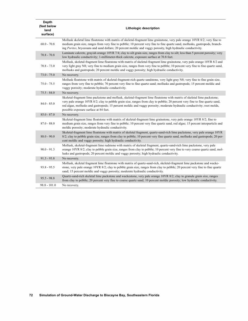
72 Simulation of Ground-Water Discharge to Biscayne Bay, Southeastern Florida
68.0 - 70.8Mollusk skeletal lime floatstone with matrix of skeletal-fragment lime grainstone, very pale orange 10YR 8/2; very fine to medium grain size, ranges from very fine to pebble; 10 percent very fine to fine quartz sand, mollusks, gastropods, branch-ing Porites, bryozoans and sand dollars; 20 percent moldic and vuggy porosity, high hydraulic conductivity.
70.8 - 70.8 Laminate calcrete, grayish orange 10YR 7/4; clay to silt grain size, ranges from clay to silt; less than 5 percent porosity; very low hydraulic conductivity; 1-millimeter-thick calcrete, exposure surface at 70.8 feet.
70.8 - 73.0 Mollusk, skeletal-fragment lime floatstone with matrix of skeletal-fragment lime grainstone, very pale orange 10YR 8/2 and very light gray N8; very fine to medium grain size, ranges from very fine to pebble; 10 percent very fine to fine quartz sand, mollusks and gastropods; 20 percent moldic and vuggy porosity; high hydraulic conductivity.
73.0 - 75.0 No recovery.
75.0 - 75.5Mollusk floatstone with matrix of skeletal-fragment-rich quartz sandstone, very light gray N8; very fine to fine grain size, ranges from very fine to pebble; 70 percent very fine to fine quartz sand; mollusks and gastropods; 15 percent moldic and vuggy porosity; moderate hydraulic conductivity.
75.5 - 84.0 No recovery.
84.0 - 85.0
Skeletal-fragment lime packstone and mollusk, skeletal-fragment lime floatstone with matrix of skeletal lime packstone; very pale orange 10YR 8/2; clay to pebble grain size, ranges from clay to pebble; 20 percent very fine to fine quartz sand, red algae, mollusks and gastropods; 15 percent moldic and vuggy porosity; moderate hydraulic conductivity; root molds, possible exposure surface at 84 feet.
85.0 - 87.0 No recovery.
87.0 - 88.0Skeletal-fragment lime floatstone with matrix of skeletal-fragment lime grainstone, very pale orange 10YR 8/2; fine to medium grain size, ranges from very fine to pebble; 10 percent very fine quartz sand, red algae; 15 percent interparticle and moldic porosity; moderate hydraulic conductivity.
88.0 - 90.0Skeletal-fragment lime floatstone with matrix of skeletal fragment, quartz-sand-rich lime packstone, very pale orange 10YR 8/2; clay to pebble grain size, ranges from clay to pebble; 10 percent very fine quartz sand, mollusks and gastropods; 20 per-cent moldic and vuggy porosity; high hydraulic conductivity.
90.0 - 91.3Mollusk, skeletal-fragment lime rudstone with matrix of skeletal fragment, quartz-sand-rich lime packstone, very pale orange 10YR 8/2; clay to pebble grain size, ranges from clay to pebble; 10 percent very fine to very coarse quartz sand, mol-lusks and gastropods; 20 percent moldic and vuggy porosity; high hydraulic conductivity.
91.3 - 93.8 No recovery.
93.8 - 95.5Mollusk, skeletal fragment lime floatstone with matrix of quartz-sand-rich, skeletal-fragment lime packstone and wacke-stone, very pale orange 10YR 8/2; clay to pebble grain size, ranges from clay to pebble; 20 percent very fine to fine quartz sand; 15 percent moldic and vuggy porosity; moderate hydraulic conductivity.
95.5 - 98.8 Quartz-sand-rich skeletal lime packstone and wackestone, very pale orange 10YR 8/2; clay to granule grain size, ranges from clay to pebble; 20 percent very fine to coarse quartz sand; 10 percent moldic porosity; low hydraulic conductivity.
98.8 - 101.0 No recovery.
Depth(feet below
land surface)
Lithologic description
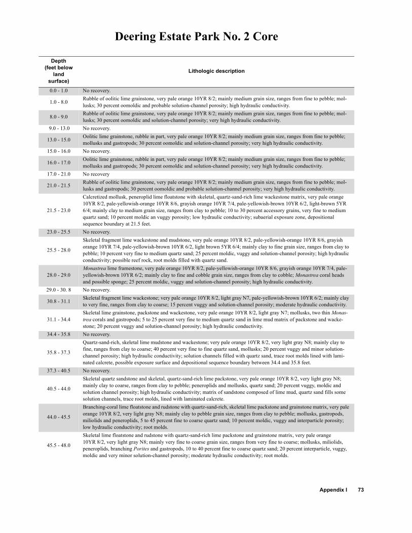
Appendix I 73
Deering Estate Park No. 2 Core
Depth(feet below
land surface)
Lithologic description
0.0 - 1.0 No recovery.
1.0 - 8.0 Rubble of oolitic lime grainstone, very pale orange 10YR 8/2; mainly medium grain size, ranges from fine to pebble; mol-lusks; 30 percent oomoldic and probable solution-channel porosity; high hydraulic conductivity.
8.0 - 9.0 Rubble of oolitic lime grainstone, very pale orange 10YR 8/2; mainly medium grain size, ranges from fine to pebble; mol-lusks; 30 percent oomoldic and solution-channel porosity; very high hydraulic conductivity.
9.0 - 13.0 No recovery.
13.0 - 15.0 Oolitic lime grainstone, rubble in part, very pale orange 10YR 8/2; mainly medium grain size, ranges from fine to pebble; mollusks and gastropods; 30 percent oomoldic and solution-channel porosity; very high hydraulic conductivity.
15.0 - 16.0 No recovery.
16.0 - 17.0 Oolitic lime grainstone, rubble in part, very pale orange 10YR 8/2; mainly medium grain size, ranges from fine to pebble; mollusks and gastropods; 30 percent oomoldic and solution-channel porosity; very high hydraulic conductivity.
17.0 - 21.0 No recovery
21.0 - 21.5 Rubble of oolitic lime grainstone, very pale orange 10YR 8/2; mainly medium grain size, ranges from fine to pebble; mol-lusks and gastropods; 30 percent oomoldic and probable solution-channel porosity; very high hydraulic conductivity.
21.5 - 23.0
Calcretized mollusk, peneroplid lime floatstone with skeletal, quartz-sand-rich lime wackestone matrix, very pale orange 10YR 8/2, pale-yellowish-orange 10YR 8/6, grayish orange 10YR 7/4, pale-yellowish-brown 10YR 6/2, light-brown 5YR6/4; mainly clay to medium grain size, ranges from clay to pebble; 10 to 30 percent accessory grains, very fine to medium quartz sand; 10 percent moldic an vuggy porosity; low hydraulic conductivity; subaerial exposure zone, depositional sequence boundary at 21.5 feet.
23.0 - 25.5 No recovery.
25.5 - 28.0
Skeletal fragment lime wackestone and mudstone, very pale orange 10YR 8/2, pale-yellowish-orange 10YR 8/6, grayish orange 10YR 7/4, pale-yellowish-brown 10YR 6/2, light brown 5YR 6/4; mainly clay to fine grain size, ranges from clay to pebble; 10 percent very fine to medium quartz sand; 25 percent moldic, vuggy and solution-channel porosity; high hydraulic conductivity; possible reef rock, root molds filled with quartz sand.
28.0 - 29.0Monastrea lime framestone, very pale orange 10YR 8/2, pale-yellowish-orange 10YR 8/6, grayish orange 10YR 7/4, pale-yellowish-brown 10YR 6/2; mainly clay to fine and cobble grain size, ranges from clay to cobble; Monastrea coral heads and possible sponge; 25 percent moldic, vuggy and solution-channel porosity; high hydraulic conductivity.
29.0 - 30. 8 No recovery.
30.8 - 31.1 Skeletal fragment lime wackestone; very pale orange 10YR 8/2, light gray N7, pale-yellowish-brown 10YR 6/2; mainly clay to very fine, ranges from clay to coarse; 15 percent vuggy and solution-channel porosity; moderate hydraulic conductivity.
31.1 - 34.4Skeletal lime grainstone, packstone and wackestone, very pale orange 10YR 8/2, light gray N7; mollusks, two thin Monas-trea corals and gastropods; 5 to 25 percent very fine to medium quartz sand in lime mud matrix of packstone and wacke-stone; 20 percent vuggy and solution-channel porosity; high hydraulic conductivity.
34.4 - 35.8 No recovery.
35.8 - 37.3
Quartz-sand-rich, skeletal lime mudstone and wackestone; very pale orange 10YR 8/2, very light gray N8; mainly clay to fine, ranges from clay to coarse; 40 percent very fine to fine quartz sand, mollusks; 20 percent vuggy and minor solution-channel porosity; high hydraulic conductivity; solution channels filled with quartz sand, trace root molds lined with lami-nated calcrete, possible exposure surface and depositional sequence boundary between 34.4 and 35.8 feet.
37.3 - 40.5 No recovery.
40.5 - 44.0
Skeletal quartz sandstone and skeletal, quartz-sand-rich lime packstone, very pale orange 10YR 8/2, very light gray N8; mainly clay to coarse, ranges from clay to pebble; peneroplids and mollusks, quartz sand; 20 percent vuggy, moldic and solution channel porosity; high hydraulic conductivity; matrix of sandstone composed of lime mud, quartz sand fills some solution channels, trace root molds, lined with laminated calcrete.
44.0 - 45.5
Branching-coral lime floatstone and rudstone with quartz-sand-rich, skeletal lime packstone and grainstone matrix, very pale orange 10YR 8/2, very light gray N8; mainly clay to pebble grain size, ranges from clay to pebble; mollusks, gastropods, miliolids and peneroplids, 5 to 45 percent fine to coarse quartz sand; 10 percent moldic, vuggy and interparticle porosity; low hydraulic conductivity; root molds.
45.5 - 48.0
Skeletal lime floatstone and rudstone with quartz-sand-rich lime packstone and grainstone matrix, very pale orange10YR 8/2, very light gray N8; mainly very fine to coarse grain size, ranges from very fine to coarse; mollusks, miliolids, peneroplids, branching Porites and gastropods, 10 to 40 percent fine to coarse quartz sand; 20 percent interparticle, vuggy, moldic and very minor solution-channel porosity; moderate hydraulic conductivity; root molds.

74 Simulation of Ground-Water Discharge to Biscayne Bay, Southeastern Florida
48.0 - 48.5 Gastropod lime floatstone with lime mudstone matrix, pale-yellowish-brown 10YR 6/2; mainly clay to silt and pebble, ranges from clay to pebble; 10 percent moldic porosity; low hydraulic conductivity; lacustrine environment.
48.5 - 48.8Skeletal lime floatstone with quartz-sand-rich skeletal lime packstone matrix, very pale orange 10YR 8/2; mainly clay to fine to coarse quartz sand, mollusks and branching corals; 15 percent moldic and vuggy porosity; moderate hydraulic con-ductivity.
48.8 - 49.2Skeletal, quartz-sand-rich lime wackestone and packstone; very pale orange 10YR 8/2; mainly clay to fine grain size, ranges from clay to fine; 20 percent very fine to coarse quartz sand, peneroplids; 10 percent moldic porosity; low hydraulic conduc-tivity.
49.2 - 50.0 Skeletal quartz-sand-rich
50.0 - 51.0Skeletal quartz sandstone, light gray N7 to very light gray N8; mainly clay and very fine to coarse grain size; ranges from clay to pebble, quartz grains are very fine to coarse; mollusks and peneroplids; 20 percent interparticle, vuggy and solution-channel porosity; moderate hydraulic conductivity; lime mud matrix.
51.0 - 54.4 No recovery.
54.4 - 57.5Skeletal quartz sandstone and quartz-sand-rich lime packstone, very pale orange 10YR 8/2, light gray N7; mainly clay and very fine to medium grain size, ranges from clay to pebble, quartz grains are very fine to medium; peneroplids, mollusks and gastropods, 40 to 70 percent quartz sand; 15 percent vuggy and interparticle porosity; low hydraulic conductivity.
57.5 - 60.5 No recovery.
60.5 - 62.5
Skeletal lime rudstone with quartz-sand-rich lime packstone matrix and quartz-sand-rich, skeletal lime wackestone, very pale orange 10YR 8/2, light gray N7; mainly clay to fine grain size, ranges from clay to pebble; peneroplids, mollusks, gas-tropods and dasyclad algae; 40 percent very fine to medium quartz sand; 20 percent moldic, interparticle and solution-chan-nel porosity; moderate hydraulic conductivity; subaerial exposure surface (depositional sequence boundary) at 60.7 feet, below surface are root molds lined with laminated calcrete.
62.5 - 70.5 No recovery.
70.5 - 71.0Skeletal, molluscan lime floatstone with quartz-sand-rich, skeletal lime grainstone, very pale orange 10YR 8/2 and light gray N7; mainly very fine to coarse grain size, ranges from fine to pebble; 10 to 30 percent very fine to fine quartz sand, mollusks and gastropods; 15 percent moldic porosity; low hydraulic conductivity.
71.0 - 74.5Skeletal, molluscan lime floatstone with quartz-sand-rich, skeletal lime packstone, very pale orange 10YR 8/2 and light gray N7; mainly clay to coarse grain size, ranges from clay to pebble; 10 to 30 percent very fine to fine quartz sand, mollusks, gastropods and one branching coral; 15 percent moldic porosity; low hydraulic conductivity.
74.5 - 75.5Skeletal, molluscan lime floatstone with quartz-sand-rich, skeletal lime packstone, very pale orange 10YR 8/2 and light gray N7; mainly clay to coarse grain size, ranges from clay to pebble; 10 to 30 percent very fine to fine quartz sand, mollusks and gastropods; 15 percent moldic porosity; low hydraulic conductivity.
75.5 - 80.5 No recovery.
80.5 - 81.5Skeletal molluscan, quartz-sand-rich lime grainstone, light gray N7; very fine to medium grain size, ranges from silt to medium; 20 percent very fine to fine quartz sand, mollusks, gastropods and red algae; 15 percent moldic and vuggy porosity; low hydraulic conductivity.
81.5 - 84.8Skeletal, molluscan lime floatstone with sleekly, quartz-sand-rich lime grainstone, very pale orange 10YR 8/2; very fine to pebble, ranges from silt to pebble; 10 to 30 percent very fine to fine quartz sand, mollusks, gastropods and red algae; 15 per-cent moldic and vuggy porosity; low hydraulic conductivity.
84.8 - 85.5Skeletal, molluscan lime floatstone with skeletal, quartz-sand-rich lime grainstone; very pale orange 10YR 8/2; very fine to pebble, ranges from silt to pebble; 10 to 30 percent very fine to fine quartz sand, mollusks, gastropods and red algae; 20 per-cent moldic and vuggy porosity; moderate hydraulic conductivity.
85.5 - 90.5 No recovery.
90.5 - 99.5
Skeletal, mollusk lime rudstone with skeletal, quartz-sand-rich lime packstone matrix, light gray N7, very pale orange 10YR 8/2; mainly clay to pebble grain size; ranges from clay to pebble; 5 to 25 percent very fine to very coarse quartz sand with uncommon very coarse quartz sand, mollusks, gastropods, red algae, sand dollars, echinoid spines; 20 percent moldic poros-ity; low hydraulic conductivity; 2-inch-thick laminations at 91.5 and 92 feet, composed of gastropod, mollusk lime rudstone with quartz-sand-rich skeletal wackestone and packstone matrix, very pale orange 10YR 8/2 and pale-yellowish-brown 10YR 6/2, possibly deposited in a lacustrine environment.
99.5 - 101.5 No recovery.
Depth(feet below
land surface)
Lithologic description

Appendix I 75
High Hope Farms Core
Depth(feet below
land surface)
Lithologic description
0.0 - 0.5 Mud and Holocene roots, pale-yellowish-brown 10YR 6/2; clay to very fine grain size; less than 5 percent microporosity; low hydraulic conductivity.
0.5 - 2.5 Highly weathered chalky limestone, very pale orange 10YR 8/2; clay to silt grain size; cerithid or serpulid tubes; 20 percent microporosity; moderate hydraulic conductivity.
2.5 - 3.5 No recovery.
3.5 - 7.5 Rubble of chalky oolitic, oomoldic lime grainstone, very pale orange 10YR 8/2; clay to medium grain size; ranges from clay to granule; gastropods and mollusks; 20 percent microporosity and moldic porosity; moderate hydraulic conductivity.
7.5 - 7.6 Rubble of laminated calcrete, light brown 5YR 5/6; clay to very fine grain size, ranges from clay to very fine; 15 percent porosity; low hydraulic conductivity; exposure surface.
7.6 - 8.8 Rubble of oomoldic, pelmoldic lime grainstone, light brown 5YR 5/6(?); 25 percent oomoldic porosity, pelmoldic and vuggy porosity; high hydraulic conductivity.
8.8 - 13.0 No recovery.
13.0 - 15.0Rubble of skeletal fragment, mollusk, gastropod lime floatstone with matrix of oomoldic, pelmoldic lime grainstone; very pale orange 10YR 8/2; very fine to fine grain size, ranges from very fine to pebble; 30 percent oomoldic, pelmoldic and vuggy porosity; high hydraulic conductivity.
15.0 - 15.7Skeletal fragment, mollusk, gastropod lime floatstone with matrix of oomoldic, pelmoldic lime grainstone, very pale orange 10YR 8/2; very fine to fine grain size, ranges from very fine to pebble; 30 percent oomoldic, pelmoldic and vuggy porosity; high hydraulic conductivity.
15.7 - 18.0 No recovery.
18.0 - 18.7Rubble of skeletal fragment lime floatstone with matrix of lime mudstone, mottled very pale orange 10YR 8/2 to grayish orange 10YR 7/4; clay grain size, ranges from clay to very fine; 20 percent root-mold, skeletal-fragment mold and vuggy porosity; high hydraulic conductivity; laminated calcrete lines root molds, probable exposure surface at 18 feet.
18.7 - 20.0
Moldic, skeletal-fragment lime floatstone with matrix of quartz-sand-rich lime mudstone, mottled very pale orange 10YR8/2 to grayish orange 10YR 7/4; clay grain size; ranges from clay to granule; 5 percent very fine to fine quartz sand, mol-lusks; 20 percent root-mold and skeletal-fragment moldic and vuggy porosity; high hydraulic conductivity; supratidal or tidal mudstones.
20.0 - 23.0 No recovery.
23.0 - 27.0
Skeletal fragment, mollusk, benthic-foraminifer lime floatstone with matrix of quartz-sand-rich, mollusk lime wackestone and packstone, mottled very pale orange 10YR 8/2 to grayish orange 10YR 7/4; clay and very fine to fine; ranges from clay to pebble; 30 percent very fine to fine quartz sand; 20 percent moldic and vuggy porosity; high hydraulic conductivity; equant limpid calcite lines interclast pores and vugs.
27.0 - 30.0
Breccia containing clasts of lime-mud-rich quartz sandstone and quartz-sand-rich lime mudstone, mottled very pale orange 10YR 8/2, grayish orange 10YR 7/4 to dark-yellowish-orange 10YR 6/6; clay and very fine to fine, ranges from clay to medium; 40 percent very fine to fine quartz sand; 20 percent interclast and vuggy porosity; very high hydraulic conductivity; equant limpid calcite lines interclast pores and vugs.
30.0 - 30.7Rubble of quartz-sand-rich lime mudstone, mottled very pale orange 10YR 8/2, grayish orange 10YR 7/4 to dark-yellowish-orange 10YR 6/6; clay and very fine to fine, ranges from clay to medium; 10 percent very fine to fine quartz sand; 20 percent interclast and vuggy porosity; very high hydraulic conductivity.
30.7 - 35.8 No recovery. 35.8 - 36.2 Rubble of limestone; probably cave.
36.2 - 37.0Gastropod, mollusk lime floatstone with matrix of quartz-sand-rich lime wackestone and packstone light gray N7; clay, very fine to fine and pebble grain size, ranges from clay to pebble; 20 to 40 percent quartz grains, dasyclad algae; 15 percent mol-dic porosity; moderate hydraulic conductivity.
37.0 - 38.0Gastropod, mollusk lime floatstone with matrix of quartz-sand-rich lime wackestone and packstone very pale orange 10YR 8/2 to very light gray N8; clay, very fine to fine and pebble grain size, ranges from clay to pebble; 20 to 40 percent quartz grains, benthic foraminifers; 15 percent moldic porosity and minor vugs; moderate hydraulic conductivity.
38.0 - 40.5 No recovery.
40.5 - 41.0Rubble of quartz-sand-rich, skeletal fragment lime grainstone, very pale orange 10YR 8/2; very fine to fine and pebble grain size; ranges from very fine to pebble; 30 percent very fine to fine quartz sand; 20 percent moldic porosity; moderate hydrau-lic conductivity.

76 Simulation of Ground-Water Discharge to Biscayne Bay, Southeastern Florida
41.0 - 42.8Mollusk lime rudstone and floatstone with matrix of quartz-sand-rich, skeletal lime grainstone, very pale orange 10YR 8/2; very fine to fine and pebble grain size, ranges from very fine to pebble; 20 to 40 percent quartz grains, mollusks, branching Porites and gastropods; 20 percent moldic porosity and minor vugs; moderate hydraulic conductivity.
42.8 - 49.5
Mollusk lime rudstone and floatstone with matrix of quartz-sand-rich, skeletal-fragment lime grainstone and skeletal-frag-ment-rich quartz sandstone, very pale orange 10YR 8/2; very fine to fine and pebble grain size, ranges from very fine to cob-ble; 20 to 60 percent very fine to fine quartz sand, mollusks, gastropods and benthic foraminifers; 20 percent moldic and vuggy porosity; moderate hydraulic conductivity; abundant calcrete line (dark-yellowish-brown 10yr 6/6) root molds between 42.8 and 47.0 feet, probable exposure surface at 42.8 feet.
49.5 - 50.5 No recovery.
50.5 - 51.3 Skeletal fragment lime grainstone, very pale orange 10YR 8/2; very fine to fine grain size, ranges from very fine to pebble; 10 percent vuggy and interparticle porosity; moderate hydraulic conductivity.
51.3 - 56.0 No recovery.
56.0 - 57.0Quartz-sand-rich, skeletal-fragment lime grainstone and skeletal-fragment-rich quartz sandstone, very pale orange 10YR8/2; very fine to medium grain size, ranges from very fine to pebble; 40 to 60 percent very fine to fine quartz grains, pener-oplids; 15 percent vuggy, moldic and interparticle porosity; moderate hydraulic conductivity.
57.0 - 58.0
Moldic, skeletal-fragment lime grainstone with matrix of quartz-sand-rich, skeletal-fragment lime grainstone and skeletal-fragment-rich quartz sandstone, very pale orange 10YR 8/2; very fine to medium and pebble grain size, ranges from very fine to pebble; 40 to 60 percent very fine to fine quartz grains, peneroplids; 15 percent vuggy, moldic and interparticle poros-ity; moderate hydraulic conductivity.
58.0 - 60.5 No recovery.
60.5 - 61.5Skeletal-fragment-rich quartz sandstone and quartz-sand-rich skeletal-fragment lime grainstone, very pale orange 10YR 8/2; very fine to fine and pebble grain size, ranges from very fine to pebble; 40 to 70 percent quartz sand, peneroplids and mol-lusks; 20 percent vuggy, moldic and interparticle porosity; moderate hydraulic conductivity.
61.5 - 62.5
Moldic mollusk lime floatstone with matrix of skeletal-fragment-rich quartz sandstone and quartz-sand-rich skeletal-frag-ment lime grainstone, very pale orange 10YR 8/2; very fine to fine and pebble grain size, ranges from very fine to pebble; 40 to 70 percent quartz sand, peneroplids and mollusks one oyster at base; 20 percent vuggy, moldic and interparticle porosity; moderate hydraulic conductivity.
62.5 - 67.0 No recovery.
67.0 - 67.2Skeletal-fragment-rich quartz sandstone, very pale orange 10YR 8/2; very fine to fine grain size, ranges from very fine to small pebble; 70 percent very fine to fine quartz sand, gastropods; 15 percent vuggy, moldic and interparticle porosity; mod-erate hydraulic conductivity.
67.2 - 70.0 No recovery.
70.0 - 70.4Oyster lime floatstone with matrix of skeletal-fragment-rich quartz sandstone, very pale orange 10YR 8/2; very fine to fine grain size, ranges from very fine to pebble; 70 percent very fine to fine quartz sand; 20 percent vuggy and interparticle porosity; moderate hydraulic conductivity.
70.4 - 72.0 Friable quartz sand, very pale orange 10YR 8/2; very fine to fine grain size, ranges from very fine to pebble; 90 percent very fine to fine quartz sand, oysters and skeletal fragments; 20 percent interparticle porosity; moderate hydraulic conductivity.
72.0 - 72.7 No recovery.
72.7 - 73.5Quartz-sand-rich, skeletal-fragment lime packstone; clay to coarse grain size, ranges from clay to pebble; 20 percent very fine to coarse quartz sand, oysters, corals, mollusks and echinoids; 15 percent vuggy porosity; moderate hydraulic conduc-tivity.
73.5 - 74.0 No recovery.
74.0 - 74.5Rubble of mollusk lime floatstone with matrix of skeletal-fragment-rich quartz sandstone, very pale orange 10YR 8/2; very fine to fine grain size, ranges from very fine to pebble; 60 percent very fine to fine quartz sand; 15 percent vuggy and inter-particle porosity; moderate hydraulic conductivity.
74.5 - 76.0Mollusk lime floatstone with matrix of skeletal fragment, quartz-sand-rich lime packstone and minor grainstone, very pale orange 10YR 8/2; very fine to coarse grain size; 10 to 20 percent very fine to coarse quartz sand, bryozoans, mollusks, red algae; 10 percent vuggy and moldic porosity; low hydraulic conductivity.
76.0 - 76.5 Rubble of mollusk lime floatstone with a matrix of skeletal-fragment quartz sandstone, very pale orange 10YR 8/2; very fine to fine grain size, ranges from very fine to pebble; 60 percent very fine to fine quartz sand, oysters; 15 percent interparticle and moldic porosity; moderate hydraulic conductivity.
76.5 - 79.0Mollusk lime floatstone with matrix of skeletal fragment, quartz-sand-rich lime packstone, very pale orange 10YR 8/2; clay to pebble grain size; 10 percent very fine to coarse quartz sand, mollusks and gastropods; 15 percent moldic and vuggy porosity; moderate hydraulic conductivity.
Depth(feet below
land surface)
Lithologic description

Appendix I 77
79.0 - 79.5Rubble of mollusk lime floatstone with matrix of skeletal fragment quartz sandstone, very pale orange 10YR 8/2; very fine to fine grain size, ranges from very fine to pebble; 70 percent very fine to fine quartz sand; 15 percent vuggy and moldic porosity; moderate hydraulic conductivity.
79.5 - 81.0 No recovery.
81.0 - 82.5Partly rubble skeletal fragment, mollusk lime floatstone with quartz-sand-rich lime packstone matrix; very fine to coarse grain size, ranges from clay to pebble; 20 percent very fine to coarse quartz sand, red algae; 15 percent moldic and vuggy porosity; moderate hydraulic conductivity.
82.5 - 85.0 No recovery.
85.0 - 85.8Rubble of mollusk, skeletal fragment lime floatstone with quartz-sand-rich lime packstone matrix; clay to medium grain size, ranges from clay to pebble; 40 percent very fine to medium quartz sand; 15 percent moldic and vuggy porosity; moder-ate hydraulic conductivity.
85.8 - 90.0 No recovery.
90.0 - 91.0Rubble of mollusk, skeletal fragment lime floatstone with quartz-sand-rich lime packstone matrix; clay to medium grain size, ranges from clay to pebble; 45 percent very fine to medium quartz sand; 15 percent moldic and vuggy porosity; moder-ate hydraulic conductivity.
91.0 - 101.0 No recovery.
Depth(feet below
land surface)
Lithologic description

78 Simulation of Ground-Water Discharge to Biscayne Bay, Southeastern Florida
Mowry Canal Core
Depth(feet below
land surface)
Lithologic description
0.0 - 1.0 Rubble of mollusk lime floatstone with peloid, oolitic lime grainstone matrix, very pale orange 10YR 8/2; fine to medium grain size, ranges from fine to pebble; 25 percent vuggy, oomoldic and pelmoldic porosity; very high hydraulic conductivity; root molds
1.0 - 3.0Rubble of bryozoan lime floatstone with peloid, oolitic lime grainstone matrix, very pale orange 10YR 8/2; fine to medium and pebble grain size, ranges from fine to pebble; branching bryozoans; 25 percent oomoldic, intraparticle and vuggy poros-ity; very high hydraulic conductivity.
3.0 - 4.0
Rubble of oolitic lime grainstone, very pale orange 10YR 8/2; fine to medium grain size; mollusks; 25 percent oomoldic, vuggy and root-mold porosity; very high hydraulic conductivity; interval contains a laminated calcrete, less than 7-millime-ters thick, that is partly a blackened soil or phosphatized; pebbles of this darkened calcrete occur above the surface, probably as a transgressive lag.
4.0 - 5.0 No recovery. 5.0 - 5.8 Muddy soil, pale-yellowish-brown 10YR 6/2; clay to very fine grain size.
5.8 - 6.8 Rubble of oolitic lime grainstone, very pale orange 10YR 8/2; medium grain size, ranges from medium to pebble; mollusks; 25 percent oomoldic and interparticle porosity; very high hydraulic conductivity.
6.8 - 12.3 Rubble of oolitic lime grainstone, very pale orange 10YR 8/2; medium grain size, ranges from medium to pebble; mollusks; 25 percent oomoldic, vuggy and interparticle porosity; very high hydraulic conductivity; Holocene black soil near top.
12.3 - 12.5 No recovery.
12.5 - 12.7 Rubble of oolitic lime grainstone, very pale orange 10YR 8/2; medium grain size, ranges from medium to pebble; mollusks; 25 percent oomoldic, vuggy and interparticle porosity; very high hydraulic conductivity.
12.7 - 12.9 No recovery.
12.9 - 15.8Rubble of oolitic lime grainstone and bryozoan lime floatstone with oolitic lime grainstone matrix, very pale orange 10YR8/2; medium grain size, ranges from medium to pebble; branching bryozoans and mollusks; 25 percent oomoldic, interparti-cle and vuggy porosity; very high hydraulic conductivity, very thin laminated calcrete at 13.1 feet.
15.8 - 17.5 Mollusk lime floatstone with oolitic lime grainstone matrix, very pale orange 10YR 8/2; medium grain size, ranges from medium to pebble; gastropods; 30 percent oomoldic, vuggy and interparticle porosity; very high hydraulic conductivity.
17.5 - 18.0 No recovery.
18.0 - 19.5Mollusk lime floatstone with burrowed, oolitic lime grainstone matrix, very pale orange 10YR 8/2; medium grain size, ranges from medium to pebble; gastropods, 5 percent fine quartz sand in matrix, root molds with laminated calcrete linings throughout interval; 30 percent oomoldic, vuggy and interparticle porosity; very high hydraulic conductivity.
19.5 - 21.8 No recovery.
21.8 - 22.6
Mollusk, peneroplid lime floatstone with oolitic grainstone matrix, very pale orange 10YR 8/2 to very light gray N8; medium and pebble grain size, ranges from medium to pebble; 5 percent fine quartz sand in matrix; 30 percent oomoldic, vuggy and interparticle porosity; very high hydraulic conductivity; root molds with laminated calcrete linings throughout interval.
22.6 - 22.8Peneroplid lime floatstone with quartz-sand-rich calcrete matrix, very pale orange 10YR 8/2 to very light gray N8; clay to fine grain size; fine quartz sand in calcrete matrix; 5 percent interparticle porosity; very low hydraulic conductivity; root molds with laminated calcrete throughout matrix, possible exposure surface at 22.6 feet.
22.8 - 26.0 No recovery.
26.0 - 28.0
Mollusk, peneroplid lime floatstone with quartz-sand-rich, skeletal fragment lime grainstone and packstone matrix, very pale orange 10YR 8/2; clay and very fine to fine, ranges from clay to pebble; peloids, 25 percent very fine to fine quartz sand; 25 percent moldic, vuggy and interparticle porosity; moderate hydraulic conductivity; Caleonassid burrows and peloid fill.
28.0 - 30.0 No recovery.
30.0 - 32.5Mollusk, peneroplid lime floatstone and rudstone with skeletal fragment, quartz-sand-rich lime packstone matrix; very pale orange 10YR 8/2; clay, very fine to fine and pebble, ranges from clay to pebble; 20 percent very fine to fine quartz sand; 25 percent moldic and very vuggy porosity; very high hydraulic conductivity; cobble-sized calcrete clasts at base of interval.
32.5 - 32.9 Laminated calcrete, grayish orange 10YR 7/4 to moderate yellowish brown 10YR 5/4; clay to very fine; 5 percent very fine quartz sand; 5 percent interparticle porosity; very low hydraulic conductivity; calcrete bounds a significant exposure surface.
32.9 - 34.2Skeletal lime floatstone with quartz-sand-rich lime packstone matrix, very pale orange 10YR 8/2 to very light gray N8; clay to medium grain size, ranges from clay to pebble; peneroplids and mollusks, 40 percent very fine to medium quartz sand; 15 percent moldic and vuggy porosity; moderate hydraulic conductivity; root molds lined with laminated calcrete.

Appendix I 79
34.2 - 35.0 No recovery.
35.0 - 37.2
Skeletal fragment, quartz-sand-rich lime grainstone and packstone and quartz sandstone; very pale orange 10YR 8/2 to light gray N7 to very light gray N8; very fine grain size, ranges from clay to pebble; peneroplids and miliolids, 40 to 60 percent very fine quartz sand; 15 percent vuggy, moldic and interparticle porosity with minor solution channels; moderate hydraulic conductivity; root molds lined with laminated calcrete near top.
37.2 - 41.0 No recovery.
41.0 - 42.0Mainly rubble of skeletal-fragment-rich quartz sand, very pale orange 10YR 8/2 to very light gray N8; very fine grain size, ranges from very fine to granule; miliolids and peneroplids, 30 percent very fine quartz sand; 20 percent vuggy and interpar-ticle porosity with minor solution channels; moderate hydraulic conductivity.
42.0 - 47.0 No recovery.
47.0 - 48.3Quartz-sand-rich, skeletal fragment lime packstone and grainstone, very pale orange 10YR 8/2 to very light gray N8; clay to very fine, ranges from clay to granule; miliolids, peneroplids, mollusks and one coral, 10 percent very fine to medium quartz sand; 20 percent vuggy and moldic porosity with minor solution channels; moderate hydraulic conductivity.
48.3 - 50.7 No recovery.
50.7 - 52.3
Skeletal lime floatstone with quartz-sand-rich, skeletal-fragment lime packstone and grainstone matrix, very pale orange 10YR 8/2 to very light gray N8; clay and very fine to medium grain size, ranges from clay to pebble; miliolids, mollusks, gastropods, dasyclad algae and stick-like Porites coral; 20 percent very fine to medium quartz sand; 20 percent vuggy, mol-dic and interparticle porosity; moderate hydraulic conductivity; possible laminated 8-millimeter-thick calcrete at 51.2 feet, packstone matrix above and grainstone matrix below calcrete.
52.3 - 54.3
Skeletal fragment, quartz-sand-rich lime packstone, mottled very pale orange 10YR 8/2 and pale-yellowish-brown 10YR6/2; clay to medium grain size, ranges from clay to pebble; 20 percent very fine to medium quartz grains, skeletal fragments, mollusks, gastropods and miliolids; 20 percent moldic and vuggy porosity with solution channels; moderate hydraulic con-ductivity; empty and quartz-sand-rich lime packstone and skeletal fragment quartz-sand-filled lime packstone, 1-millimeter-thick laminated calcrete lines solution channels.
54.3 - 55.0Gastropod lime floatstone with quartz-sand-rich lime packstone matrix, pale-yellowish-brown 10YR 6/2; fine to medium grain size; gastropods, 20 to 40 percent fine to medium quartz sand; 20 percent moldic porosity; moderate hydraulic conduc-tivity; probably lacustrine depositional environment.
55.0 - 55.8 No recovery.
55.8 - 57.0Gastropod lime floatstone with quartz-sand-rich lime packstone matrix, pale-yellowish-brown 10YR 6/2; clay to medium grain size; gastropods, 20 to 40 percent fine to medium quartz sand; 20 percent moldic porosity; moderate hydraulic conduc-tivity; probably lacustrine depositional environment.
57.0 - 59.0
Skeletal fragment lime floatstone with quartz-sand-rich lime packstone and skeletal, quartz-sand-rich packstone; very pale orange 10YR 8/2 to very light gray N8; clay to medium grain size, ranges from clay to pebble; gastropods, mollusks, miliol-ids and peneroplids; 20 to 40 percent very fine to medium quartz sand; 20 percent moldic and vuggy porosity; moderate hydraulic conductivity.
59.0 - 60.0
Mollusk, skeletal lime floatstone with skeletal fragment quartz sandstone matrix; clay to medium grain size ranges from clay to pebble; miliolids, mollusks and peneroplids, 40 percent very fine to medium quartz grains; quartz sandstone contains a lime mud matrix; 20 percent vuggy and moldic porosity with solution channels; moderate hydraulic conductivity; truncated root molds at top of interval and root molds with laminated calcrete linings (grayish orange 10YR 7/4) throughout interval, probable exposure surface at top of interval
60.0 - 60.5 No recovery.
60.5 - 62.5
Skeletal fragment, quartz sandstone with lime mud matrix, very pale orange 10YR 8/2 to grayish orange 10YR 7/4 to very light gray N8; clay and fine to medium; ranges from clay to granule; mollusks and miliolids, 20 to 40 percent fine to medium quartz grains; 20 percent moldic and vuggy porosity with minor solution channels; moderate hydraulic conductivity; interval riddled with root molds lined with laminated calcrete.
62.5 - 63.0 Skeletal lime grainstone, very light gray N8 and grayish orange 10YR 7/4; fine grain size, ranges from very fine to pebble; miliolids and peneroplids, 10 percent very fine quartz sand; 10 percent interparticle porosity; low hydraulic conductivity.
63.0 - 70.5 No recovery.
70.5 - 71.4
Mollusk skeletal lime floatstone with skeletal lime grainstone matrix, very pale orange 10YR 8/2; very fine to medium and pebble grain size, ranges from very fine to pebble; stick-like Porites corals and dasyclad algae, 40 percent very fine to medium quartz sand; 30 percent interparticle, moldic and large vuggy porosity with solution channels; high hydraulic con-ductivity
71.4 - 72.5Skeletal fragment lime grainstone, very pale orange 10YR 8/2; fine to medium grain size, ranges from very fine to granule; peneroplids, 10 percent fine quartz sand; 20 percent interparticle porosity with minor solution channels; moderate hydraulic conductivity.
Depth(feet below
land surface)
Lithologic description

80 Simulation of Ground-Water Discharge to Biscayne Bay, Southeastern Florida
72.5 - 75.4 No recovery.
75.4 - 76.2Skeletal fragment lime grainstone, very pale orange 10YR 8/2; fine to medium grain size, ranges from very fine to granule; peneroplids, 10 percent fine quartz sand; 20 percent interparticle porosity with minor solution channels; moderate hydraulic conductivity.
76.2 - 77.0
Skeletal fragment lime floatstone with quartz-sand-rich, skeletal lime grainstone matrix, very pale orange 10YR 8/2 and very light gray N8; very fine to medium and pebble grain size, ranges from very fine to pebble; mollusks, dasyclad algae and peneroplids, 10 to 40 percent very fine to fine quartz sand; 30 percent interparticle porosity with solution channels; high hydraulic conductivity.
77.0 - 79.5
Skeletal fragment lime floatstone with quartz-sand-rich, skeletal lime grainstone matrix, very pale orange 10YR 8/2 and very light gray N8; very fine to medium and pebble grain size, ranges from very fine to pebble; mollusks, dasyclad algae and peneroplids, 10 to 40 percent very fine to fine quartz sand; 20 percent moldic and interparticle porosity; moderate hydraulic conductivity.
79.5 - 80.5 No recovery.
80.5 - 81.0
Rubble of skeletal fragment lime floatstone with quartz-sand-rich, skeletal lime grainstone matrix, very pale orange 10YR8/2 and very light gray N8; very fine to medium and pebble grain size, ranges from very fine to pebble; mollusks, dasyclad algae and peneroplids, 10 to 40 percent very fine to fine quartz sand; 20 percent moldic and interparticle porosity; moderate hydraulic conductivity.
81.0 - 83.8Skeletal lime rudstone with quartz-sand-rich, skeletal lime grainstone, very pale orange 10 YR 8/2; very fine to pebble grain size, ranges from very fine to pebble; mollusks and echinoids, 10 to 40 percent very fine to fine quartz sand; 20 percent mol-dic and interparticle porosity; moderate hydraulic conductivity.
83.8 - 86.0 No recovery.
86.0 - 86.2
Skeletal lime floatstone with quartz-sand-rich, lime packstone, pale-yellowish-brown 10 YR 6/2; clay to medium grain size, ranges from clay to pebble; mollusks and echinoids, 20 percent very fine to fine quartz sand; 20 percent moldic and interpar-ticle porosity; moderate hydraulic conductivity; root molds lined with laminated calcrete, exposure surface near or at top of interval at 86 feet.
86.2 - 86.6Skeletal quartz-sand-rich lime wackestone, pale-yellowish-brown 10YR 6/2; clay to very fine, ranges from clay to coarse; 1 percent very fine to fine quartz sand; 10 percent fenestral(?) porosity; low hydraulic conductivity; root molds lined with lam-inated calcrete.
86.6 - 87.3Mollusk lime floatstone with quartz-sand-rich, skeletal lime packstone matrix, very pale orange 10YR 8/2; clay to pebble grain size; mollusks, miliolids, 40 percent very fine to fine quartz sand; 15 percent moldic and root mold porosity; low hydraulic conductivity; root molds lined with laminated calcrete.
87.3 - 88.0Mollusk lime floatstone with quartz-sand-rich, skeletal lime packstone matrix, very pale orange 10YR 8/2; clay to pebble grain size; mollusks, miliolids, 40 percent very fine to fine quartz sand; 20 percent moldic and root mold porosity; moderate hydraulic conductivity; root molds lined with laminated calcrete.
88.0 - 90.5 No recovery.
90.5 - 90.9 Skeletal lime grainstone, very pale orange 10YR 8/2; very fine to fine, ranges from very fine to coarse; mollusks and miliol-ids; 10 percent moldic porosity; low hydraulic conductivity.
90.9 - 91.6Skeletal lime floatstone with quartz-sand-rich lime packstone matrix, very pale orange 10YR 8/2; clay to coarse, ranges from clay to pebble; mollusks, 20 to 40 percent very fine to fine quartz sand, 15 percent moldic porosity with solution chan-nels; moderate hydraulic conductivity.
91.6 - 94.0
Mollusk lime floatstone with quartz-sand-rich, skeletal fragment lime packstone and grainstone, very pale orange 10YR 8/2 to very light gray N8; clay to fine grain size, ranges from clay to pebble; mollusks, gastropods, miliolids and peneroplids, 40 percent very fine to medium quartz sand; 20 percent moldic and vuggy solution channels with minor solution channels; high hydraulic conductivity.
94.0 - 95.4Skeletal lime floatstone and rudstone with skeletal, quartz-sand-rich lime packstone, very pale orange 10YR 8/2 to very light gray N8; clay to pebble grain size, ranges from clay to pebble; mollusks, 10 percent fine to medium quartz sand; 25 percent vuggy and moldic porosity; moderate hydraulic conductivity
95.4 - 96.0Rubble of skeletal fragment, quartz-sand-rich lime grainstone, very pale orange 10YR 8/2 to very light gray N8; very fine to medium grain size, ranges from very fine to medium; 10 percent very fine quartz sand; 10 percent interparticle porosity; low hydraulic conductivity.
96.0 - 100.5Molluscan lime floatstone and rudstone with quartz-sand-rich, skeletal lime packstone, very pale orange 10YR 8/2 to very light gray N8; clay to pebble grain size; ranges from clay to pebble; mollusks and gastropods, 10 to 30 percent very fine to medium quartz sand; 20 percent moldic and vuggy porosity; moderate hydraulic conductivity.
Depth(feet below
land surface)
Lithologic description

Appendix I 81
Peacock Park
Depth(feet below
land surface)
Lithologic description
0.0 - 1.0 Quartz-sand-rich soil, dark-yellowish-brown 10YR 4/2; mainly clay and fine to medium grain size, ranges from clay to coarse; roots; 20 percent interparticle porosity; low hydraulic conductivity.
1.0 - 2.0 Rubble of oolitic lime grainstone, very pale orange 10YR 8/2; mainly medium grain size; 25 percent oomoldic and probable solution-channel porosity; high hydraulic conductivity.
2.0 - 3.0 Loose quartz sand, very pale orange 10YR 8/2, grayish orange 10YR 7/4; mainly fine to medium, ranges from fine to medium; 25 percent interparticle porosity; moderate hydraulic conductivity; bay sediments(?).
3.0 - 4.0 No recovery.
4.0 - 5.0 Silty mudstone, very pale orange 10YR 8/2, pale-yellowish-brown 10YR 6/2, brownish gray 5YR 4/1; mainly clay to silt; roots; 5 percent interparticle porosity; very low hydraulic conductivity; bay sediments(?)
5.0 - 5.5 Peat; black N1; mainly clay to silt; roots; 25 percent interparticle porosity; very low hydraulic conductivity; bay sedi-ments(?)
5.5 - 8.5 Loose quartz sand, pale-yellowish-brown 10YR 6/2, light gray N7; mainly fine to medium grain size, ranges from very fine to coarse; caved grains; 25 percent interparticle porosity; moderate hydraulic conductivity; mainly caved quartz sand (?)
8.5 - 9.0 Calcretized oolitic lime grainstone, very pale orange 10YR 8/2, pale-yellowish-brown 10YR 6/2; medium grain size; 25 per-cent oomoldic and solution-channel porosity; high hydraulic conductivity.
9.0 - 11.0 No recovery.
11.0 - 13.0 Loose quartz sand, very light gray N7; mainly fine to medium grain size, ranges from fine to coarse; caved particles and roots; 25 percent interparticle porosity; moderate hydraulic conductivity.
13.0 - 13.8 Rubble of oolitic lime grainstone, very pale orange 10YR 8/2; mainly fine grain size; ranges from fine to pebble; mollusks and branching bryozoans 25 percent oomoldic and solution-channel porosity; high hydraulic conductivity.
13.8 - 15.0Rubble of oolitic lime grainstone, very pale orange 10YR 8/2, grayish orange 10YR 7/4, moderate yellowish brown 10 YR 5/4; mainly fine grain size; ranges from fine to pebble; mollusks and branching bryozoans 25 percent oomoldic and solution-channel porosity; high hydraulic conductivity.
15.0 - 16.0 Loose quartz sand, very light gray N7; mainly fine to medium grain size, ranges from fine to coarse; 25 percent interparticle porosity; moderate hydraulic conductivity.
16.0 - 18.0Rubble of oolitic lime grainstone, very pale orange 10YR 8/2, grayish orange 10YR 7/4, moderate yellowish brown 10YR5/4; mainly fine grain size, ranges from fine to medium; 25 percent oomoldic and solution-channel porosity; high hydraulic conductivity.
18.0 - 23.2 No recovery.
23.2 - 24.0Rubble of sandstone cemented with calcite and oolitic lime grainstone, sample is probably cave, very pale orange 10 YR8/2, grayish orange 10YR 7/4, moderate yellowish brown 10YR 5/4; mainly fine grain size, ranges from fine to medium; 25 percent oomoldic, interparticle and vuggy porosity; high hydraulic conductivity.
24.0 - 25.0 No recovery.
25.0 - 25.5 Rubble of oolitic lime grainstone, very pale orange 10YR 8/2, grayish orange 10YR 7/4; mainly fine grain size, ranges from fine to pebble; branching bryozoans and mollusks; 25 percent oomoldic porosity; high hydraulic conductivity.
25.5 - 30.0 No recovery.
30.0 - 30.8Skeletal-fragment lime grainstone, very pale orange 10YR 8/2, grayish orange 10YR 7/4, dark-yellowish-orange 10YR 6/6; mainly fine to medium grain size, ranges from very fine to granule; 35 percent vuggy, moldic, interparticle and solution-channel porosity; very high hydraulic conductivity; probable exposure surface between 25.5 and 30 feet.
30.8 - 31.7Skeletal-fragment lime rudstone with skeletal-fragment lime grainstone matrix; very pale orange 10YR 8/2, grayish-orange 10YR 7/4, dark-yellowish-orange 10 YR 6/6; mainly fine to granule grain size; 35 percent vuggy, moldic, interparticle and solution-channel porosity; very high hydraulic conductivity.
31.7 - 32.7Skeletal-fragment lime rudstone with skeletal-fragment lime grainstone matrix; very pale orange 10YR 8/2, grayish-orange 10YR 7/4, dark-yellowish-orange 10 YR 6/6; mainly medium to pebble grain size; 35 percent vuggy, moldic, interparticle and solution-channel porosity; very high hydraulic conductivity.
32.7 - 34.0 Monastrea lime framestone, very pale orange 10YR 8/2; mainly cobble grain size; 25 percent intraparticle porosity; very high hydraulic conductivity.
34.0 - 35.0 No recovery.
35.0 - 36.0 Rubble of coral lime framestone, very pale orange 10YR 8/2; mainly clay and pebble and cobble, ranges from clay to cob-ble; 25 percent intraparticle porosity; very high hydraulic conductivity.

82 Simulation of Ground-Water Discharge to Biscayne Bay, Southeastern Florida
36.0 - 40.8 No recovery.
40.8 - 41.8 Rubble of skeletal lime packstone, very pale orange 10YR 8/2, grayish orange 10YR 7/4; mainly clay to pebble; ranges from clay to pebble; 20 percent moldic and vuggy porosity; high hydraulic conductivity; possible cave.
41.8 - 43.0Friable calcareous quartz sandstone; very pale orange 10YR 8/2, pale-yellowish-orange 10YR 6/6; grayish-orange 10YR7/4; mainly very fine to fine grain size, ranges from very fine to medium; 20 percent interparticle porosity; moderate hydrau-lic conductivity.
43.0 - 45.5Rubble of skeletal lime grainstone and packstone and oolitic lime grainstone, very pale orange 10YR 8/2, grayish-orange 10YR 7/4; mainly clay to pebble grain size, ranges from clay to pebble; 20 percent moldic, vuggy and interparticle porosity; high hydraulic conductivity; at least some of the rubbly limestone is cave (oolitic lime grainstone)
45.5 - 51.0 No recovery. 51.0 -51.5 Rubble of caved limestone.
51.5 - 52.0 Diplora coral lime framestone, very pale orange 10YR 8/2; mainly cobble grain size; 30 percent intraparticle porosity; very high hydraulic conductivity.
52.0 - 61.0 Rubble of caved limestone.
61.0 - 62.5
Skeletal fragment lime wackestone, packstone and grainstone, mottled combination of very pale orange 10YR 8/2, pale-yel-lowish-orange 10YR 8/6, grayish orange 10YR 7/4, and very light gray N7; mainly clay to medium grain size; ranges from clay to pebble; peloids, mollusks, gastropods and echinoid spines; 25 percent moldic, root-mold and minor solution-channel porosity; high hydraulic conductivity; mottled colors, root molds and solution channels suggest exposure surface between 52 and 61 feet.
62.5 - 71.0 No recovery.
71.0 - 71.5
Rubble of skeletal fragment lime wackestone, packstone and grainstone, mottled combination of very pale orange 10YR 8/2, pale-yellowish-orange 10YR 8/6, grayish orange 10YR 7/4, and very light gray N7; mainly clay to medium grain size; ranges from clay to pebble; peloids, mollusks, gastropods and echinoid spines; 25 percent moldic, root-mold and minor solu-tion-channel porosity; high hydraulic conductivity.
71.5 - 72.0
Skeletal fragment lime wackestone and packstone, mottled combination of very pale orange 10YR 8/2, pale-yellowish-orange 10YR 8/6, grayish orange 10YR 7/4, and very light gray N7; mainly clay to medium grain size; ranges from clay to pebble; peloids, mollusks, miliolids and gastropods; 25 percent moldic, root-mold and minor solution-channel porosity; high hydraulic conductivity.
72.0 - 73.0Red algae, skeletal fragment, quartz-sand-rich lime grainstone; very pale orange 10YR 8/2; light gray N8; mainly very fine to coarse grain size. ranges from very fine to pebble; 10 percent fine to medium quartz sand; red algae and mollusks; 20 per-cent moldic and interparticle porosity; moderate hydraulic conductivity.
73.0 - 76.2 No recovery.
76.2 - 77.6Skeletal fragment, red algae, quartz-sand-rich lime grainstone; very light gray N7; light gray N8; mainly very fine to coarse grain size. ranges from very fine to pebble; 20 percent fine to medium quartz sand; mollusks; 15 percent moldic and interpar-ticle porosity; moderate hydraulic conductivity.
77.6 - 78.0Red algae lime floatstone with quartz-sand-rich, skeletal lime packstone matrix, mollusks, very pale orange 10YR 8/2, light gray N7; mainly clay to granule, ranges from clay to pebble; 20 percent fine to medium quartz sand, mollusks; 15 percent moldic, intergranular and vuggy porosity; moderate hydraulic conductivity.
78.0 - 81.0 No recovery.
81.0 - 82.3
Red algae, mollusk lime rudstone and floatstone with quartz-sand-rich, skeletal lime packstone matrix, light gray N7, very pale orange 10YR 8/2, grayish orange 10YR 7/4; mainly clay to pebble grain size, ranges from clay to pebble; 20 percent fine to medium quartz sand and minor coarse quartz sand; 15 percent moldic and vuggy porosity; moderate hydraulic con-ductivity.
82.3 - 83.5Skeletal fragment, quartz-sand-rich lime grainstone, yellowish gray 5Y 8/1; mainly fine to medium grain size, ranges from very fine to medium; 15 to 25 percent very fine to fine quartz sand; mollusks, gastropods; 25 percent moldic and interparti-cle porosity; moderate hydraulic conductivity.
83.5 - 84.9Lime mudstone, wackestone and packstone; very pale orange 10YR 8/2; mainly clay to very fine grain size, 10 percent very fine to fine quartz sand gastropods, mollusks; 15 percent moldic and root-mold porosity; low hydraulic conductivity; supratidal or intertidal environment, root molds, subaerial exposure surface at 83.5 feet.
84.9 - 85.2 Skeletal, quartz-sand-rich lime packstone; very pale orange 10YR 8/2; mainly clay to medium grain size; 20 percent very fine to fine quartz sand; 15 percent moldic porosity; moderate hydraulic conductivity.
85.2 - 88.0 No recovery.
Depth(feet below
land surface)
Lithologic description

Appendix I 83
88.0 - 89.0Skeletal, quartz-sand-rich lime grainstone, very light gray N7, very pale orange 10YR 8/2; mainly very fine to medium grain size, ranges from very fine to coarse; 20 percent very fine to fine quartz sand, gastropods, mollusks; 20 percent moldic and interparticle porosity; moderate hydraulic conductivity.
89.0 - 89.5Mollusk lime rudstone with quartz sand-rich, skeletal lime packstone matrix, very light gray N7, very pale orange 10YR 8/2; mainly clay to fine and pebble grain size, ranges from clay to pebble; 20 percent very fine to fine quartz sand; 15 percent moldic porosity; moderate hydraulic conductivity.
89.5 - 91.0
Skeletal, mollusk, quartz-sand-rich lime packstone and grainstone and minor lime floatstone with skeletal, quartz-sand-rich matrix; very light gray N7, very pale orange 10YR 8/2; mainly clay to medium grain size; ranges from clay to pebble; 30 percent very fine to fine quartz sand, mollusks, red algae; 15 percent moldic and interparticle porosity; moderate hydraulic conductivity.
91.0 - 95.0 No recovery. 95.0 - 95.5 Rubble of caved limestone.
95.5 - 100.0
Skeletal fragment, quartz-sand-rich lime grainstone and minor lime packstone, very light gray N7, very pale orange 10YR8/2; mainly very fine to medium grain size, ranges from clay to pebble; 10 to 20 percent very fine to fine quartz sand and minor medium quartz sand, mollusks, gastropods, miliolids; 20 percent moldic, interparticle and vuggy porosity; moderate hydraulic conductivity.
100.0 - 101.0 No recovery.
Depth(feet below
land surface)
Lithologic description

84 Simulation of Ground-Water Discharge to Biscayne Bay, Southeastern Florida

Appendix II 85
Appendix II. Field Data Collected as Part of this Study
[--, not reported (time) or not measured]
Wellname Transect Date Time
Fluidconductivity
(microsiemensper centimeter)
Chloride concentra-
tion(milligrams per liter)
Depth to water(feet)
G-906 Deering Estate 03-02-98 1700 50,200 18,600 8.68
G-906 Deering Estate 04-03-98 1305 49,700 19,100 9.10
G-906 Deering Estate 05-04-98 1115 49,800 19,100 9.32
G-906 Deering Estate 06-01-98 1110 48,700 -- 8.83
G-906 Deering Estate 07-06-98 1139 47,900 -- 8.86
G-906 Deering Estate 08-06-98 0902 49,400 -- 8.60
G-906 Deering Estate 09-03-98 0907 45,200 -- 8.32
G-906 Deering Estate 10-06-98 0827 50,100 -- 8.42
G-906 Deering Estate 11-18-98 0911 50,300 -- 8.40
G-906 Deering Estate 12-18-98 1342 -- -- 8.69
G-906 Deering Estate 02-11-99 1238 50,000 -- 8.89
G-906 Deering Estate 03-03-99 1000 -- -- 8.28
G-911 Deering Estate 04-03-98 1308 4,920 -- 9.45
G-911 Deering Estate 05-04-98 1117 6,080 1,800 9.68
G-911 Deering Estate 06-01-98 1216 -- -- 9.10
G-911 Deering Estate 07-06-98 1207 6,460 -- 9.28
G-911 Deering Estate 08-06-98 0948 6,510 -- 9.04
G-911 Deering Estate 09-03-98 0903 7,750 -- 8.70
G-911 Deering Estate 10-06-98 0824 8,500 -- 8.85
G-911 Deering Estate 11-18-98 0905 8,340 -- 8.88
G-911 Deering Estate 02-11-99 1301 5,680 -- 9.24
G-911 Deering Estate 03-03-99 1003 -- -- 8.64
G-912 Deering Estate 03-02-98 1710 970 145 8.57
G-912 Deering Estate 04-03-98 1311 979 150 8.93
G-912 Deering Estate 05-04-98 1120 1,024 160 9.16
G-912 Deering Estate 06-01-98 1152 1,124 -- 8.60
G-912 Deering Estate 07-06-98 1203 942 -- 8.74

86 Simulation of Ground-Water Discharge to Biscayne Bay, Southeastern Florida
G-912 Deering Estate 08-06-98 0942 1,078 -- 8.51
G-912 Deering Estate 09-03-98 0915 1,260 -- 8.18
G-912 Deering Estate 10-06-98 0815 1,186 -- 8.30
G-912 Deering Estate 11-18-98 0857 1,152 -- 8.32
G-912 Deering Estate 02-11-99 1255 1,054 -- 8.70
G-912 Deering Estate 03-03-99 1005 -- -- 8.10
G-913 Deering Estate 04-03-98 1313 900 -- 9.43
G-913 Deering Estate 05-04-98 1122 899 -- 9.60
G-913 Deering Estate 06-01-98 1228 909 -- 9.05
G-913 Deering Estate 07-06-98 1215 876 -- 9.18
G-913 Deering Estate 08-06-98 0950 941 -- 8.98
G-913 Deering Estate 09-03-98 0906 963 -- 8.64
G-913 Deering Estate 10-06-98 0822 1,018 -- 8.82
G-913 Deering Estate 11-18-98 0902 993 -- 8.80
G-913 Deering Estate 02-11-99 1303 984 -- 9.18
G-913 Deering Estate 03-03-99 1008 -- -- 8.62
G-916 Deering Estate 03-02-98 1700 643 30 9.18
G-916 Deering Estate 04-03-98 1317 -- -- 9.68
G-916 Deering Estate 05-04-98 1125 -- -- 9.82
G-916 Deering Estate 06-01-98 1205 -- -- 9.33
G-916 Deering Estate 07-06-98 1205 614 -- 9.36
G-916 Deering Estate 08-06-98 0946 636 -- 9.22
G-916 Deering Estate 09-03-98 0919 625 -- 8.90
G-916 Deering Estate 10-06-98 0820 664 -- 8.98
G-916 Deering Estate 11-18-98 0900 671 -- 9.08
G-916 Deering Estate 02-11-99 1316 658 -- 9.40
G-916 Deering Estate 03-03-99 1010 -- -- 8.90
G-929 Deering Estate 03-02-98 1530 15,040 4,800 2.74
G-929 Deering Estate 04-03-98 1237 14,620 4,800 2.95
Wellname Transect Date Time
Fluidconductivity
(microsiemensper centimeter)
Chloride concentra-
tion(milligrams per liter)
Depth to water(feet)

Appendix II 87
G-929 Deering Estate 05-04-98 1150 18,700 6,300 3.31
G-929 Deering Estate 06-01-98 1305 21,300 -- 2.28
G-929 Deering Estate 07-06-98 0957 15,100 -- 2.68
G-929 Deering Estate 08-06-98 0745 20,000 -- 2.26
G-929 Deering Estate 09-03-98 0753 20,800 -- 1.90
G-929 Deering Estate 10-06-98 1024 17,100 -- 1.70
G-929 Deering Estate 11-17-98 1522 16,600 -- 3.15
G-929 Deering Estate 02-11-99 1133 15,200 -- 2.84
G-929 Deering Estate 03-03-99 0935 -- -- 1.80
G-930 Deering Estate 03-02-98 1530 2,587 620 2.48
G-930 Deering Estate 04-03-98 1238 2,846 720 2.78
G-930 Deering Estate 05-04-98 1151 2,750 700 3.16
G-930 Deering Estate 06-01-98 1307 2,320 -- 2.11
G-930 Deering Estate 07-06-98 1001 4,910 -- 2.53
G-930 Deering Estate 08-06-98 0750 3,834 -- 2.06
G-930 Deering Estate 09-03-98 0756 2,950 -- 1.72
G-930 Deering Estate 10-06-98 1025 10,920 -- 1.53
G-930 Deering Estate 11-17-98 1525 4,500 -- 2.96
G-930 Deering Estate 02-11-99 1136 4,530 -- 2.65
G-930 Deering Estate 03-03-99 0936 -- -- 1.60
G-931 Deering Estate 03-02-98 1555 1,280 235 2.51
G-931 Deering Estate 04-03-98 1240 1,344 250 2.79
G-931 Deering Estate 05-04-98 1153 1,370 260 3.15
G-931 Deering Estate 06-01-98 1317 1,278 -- 2.08
G-931 Deering Estate 07-06-98 1007 1,230 -- 2.57
G-931 Deering Estate 08-06-98 0754 1,247 -- 2.06
G-931 Deering Estate 09-03-98 0757 1,280 -- 1.74
G-931 Deering Estate 10-06-98 1026 1,307 -- 1.54
G-931 Deering Estate 11-17-98 1518 1,293 -- 2.97
Wellname Transect Date Time
Fluidconductivity
(microsiemensper centimeter)
Chloride concentra-
tion(milligrams per liter)
Depth to water(feet)

88 Simulation of Ground-Water Discharge to Biscayne Bay, Southeastern Florida
G-931 Deering Estate 02-11-99 1138 1,232 -- 2.70
G-931 Deering Estate 03-03-99 0938 -- -- 1.60
G-3629 Mowry Canal 03-04-98 -- 51,300 17,300 --
G-3629 Mowry Canal 04-01-98 -- 51,000 19,300 --
G-3629 Mowry Canal 05-08-98 -- 49,800 18,200 --
G-3629 Mowry Canal 06-03-98 -- 52,800 -- --
G-3629 Mowry Canal 07-07-98 -- 50,900 -- --
G-3629 Mowry Canal 08-03-98 -- 51,200 -- --
G-3629 Mowry Canal 09-01-98 -- 49,800 -- --
G-3629 Mowry Canal 10-08-98 -- 50,000 -- --
G-3629 Mowry Canal 11-09-98 -- 51,200 -- --
G-3629 Mowry Canal 02-10-99 -- 51,000 -- --
G-3631 Mowry Canal 03-04-98 -- 51,400 19,600 --
G-3631 Mowry Canal 04-01-98 -- 52,000 19,800 --
G-3631 Mowry Canal 05-08-98 -- 50,900 19,700 --
G-3631 Mowry Canal 06-03-98 -- 51,400 -- --
G-3631 Mowry Canal 07-07-98 -- 51,400 -- --
G-3631 Mowry Canal 08-03-98 -- 51,200 -- --
G-3631 Mowry Canal 09-01-98 -- 51,200 -- --
G-3631 Mowry Canal 10-08-98 -- 52,200 -- --
G-3631 Mowry Canal 11-09-98 -- 52,500 -- --
G-3631 Mowry Canal 02-10-99 -- 52,200 -- --
G-3632 Mowry Canal 03-04-98 -- 49,900 18,900 --
G-3632 Mowry Canal 04-01-98 -- 50,400 19,100 --
G-3632 Mowry Canal 05-08-98 -- 49,900 19,100 --
G-3632 Mowry Canal 06-03-98 -- 47,500 -- --
G-3632 Mowry Canal 07-07-98 -- 49,700 -- --
G-3632 Mowry Canal 08-03-98 -- 49,800 -- --
G-3632 Mowry Canal 09-01-98 -- 50,000 -- --
Wellname Transect Date Time
Fluidconductivity
(microsiemensper centimeter)
Chloride concentra-
tion(milligrams per liter)
Depth to water(feet)

Appendix II 89
G-3632 Mowry Canal 10-08-98 -- 49,700 -- --
G-3632 Mowry Canal 11-09-98 -- 48,100 -- --
G-3632 Mowry Canal 02-10-99 -- 50,800 -- --
G-3634 Mowry Canal 03-04-98 -- 52,200 19,800 --
G-3634 Mowry Canal 04-01-98 -- 52,400 20,000 --
G-3634 Mowry Canal 05-08-98 -- 51,800 20,000 --
G-3634 Mowry Canal 06-03-98 -- 51,400 -- --
G-3634 Mowry Canal 07-07-98 -- 51,800 -- --
G-3634 Mowry Canal 08-03-98 -- 51,300 -- --
G-3634 Mowry Canal 09-01-98 -- 51,700 -- --
G-3634 Mowry Canal 10-08-98 -- 51,900 -- --
G-3634 Mowry Canal 11-09-98 -- 51,200 -- --
G-3634 Mowry Canal 02-10-99 -- 52,800 -- --
G-3635 Mowry Canal 03-04-98 -- 49,000 18,500 --
G-3635 Mowry Canal 04-01-98 -- 49,000 18,400 --
G-3635 Mowry Canal 05-08-98 -- 48,600 18,500 --
G-3635 Mowry Canal 06-03-98 -- 48,600 -- --
G-3635 Mowry Canal 07-07-98 -- 49,100 -- --
G-3635 Mowry Canal 08-03-98 -- 48,700 -- --
G-3635 Mowry Canal 09-01-98 -- 49,200 -- --
G-3635 Mowry Canal 10-08-98 -- 49,100 -- --
G-3635 Mowry Canal 11-09-98 -- 46,300 -- --
G-3635 Mowry Canal 02-10-99 -- 48,800 -- --
G-3636 Mowry Canal 03-04-98 -- 52,000 19,900 --
G-3636 Mowry Canal 04-01-98 -- 52,600 20,000 --
G-3636 Mowry Canal 05-08-98 -- 51,700 19,900 --
G-3636 Mowry Canal 06-03-98 -- 51,400 -- --
G-3636 Mowry Canal 07-07-98 -- 51,900 -- --
G-3636 Mowry Canal 08-03-98 -- 51,900 -- --
Wellname Transect Date Time
Fluidconductivity
(microsiemensper centimeter)
Chloride concentra-
tion(milligrams per liter)
Depth to water(feet)
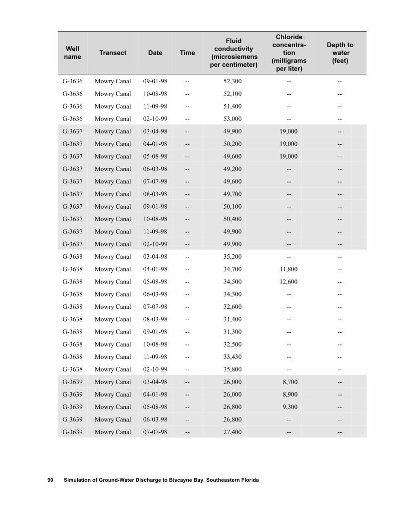
90 Simulation of Ground-Water Discharge to Biscayne Bay, Southeastern Florida
G-3636 Mowry Canal 09-01-98 -- 52,300 -- --
G-3636 Mowry Canal 10-08-98 -- 52,100 -- --
G-3636 Mowry Canal 11-09-98 -- 51,400 -- --
G-3636 Mowry Canal 02-10-99 -- 53,000 -- --
G-3637 Mowry Canal 03-04-98 -- 49,900 19,000 --
G-3637 Mowry Canal 04-01-98 -- 50,200 19,000 --
G-3637 Mowry Canal 05-08-98 -- 49,600 19,000 --
G-3637 Mowry Canal 06-03-98 -- 49,200 -- --
G-3637 Mowry Canal 07-07-98 -- 49,600 -- --
G-3637 Mowry Canal 08-03-98 -- 49,700 -- --
G-3637 Mowry Canal 09-01-98 -- 50,100 -- --
G-3637 Mowry Canal 10-08-98 -- 50,400 -- --
G-3637 Mowry Canal 11-09-98 -- 49,900 -- --
G-3637 Mowry Canal 02-10-99 -- 49,900 -- --
G-3638 Mowry Canal 03-04-98 -- 35,200 -- --
G-3638 Mowry Canal 04-01-98 -- 34,700 11,800 --
G-3638 Mowry Canal 05-08-98 -- 34,500 12,600 --
G-3638 Mowry Canal 06-03-98 -- 34,300 -- --
G-3638 Mowry Canal 07-07-98 -- 32,600 -- --
G-3638 Mowry Canal 08-03-98 -- 31,400 -- --
G-3638 Mowry Canal 09-01-98 -- 31,300 -- --
G-3638 Mowry Canal 10-08-98 -- 32,500 -- --
G-3638 Mowry Canal 11-09-98 -- 33,430 -- --
G-3638 Mowry Canal 02-10-99 -- 35,800 -- --
G-3639 Mowry Canal 03-04-98 -- 26,000 8,700 --
G-3639 Mowry Canal 04-01-98 -- 26,000 8,900 --
G-3639 Mowry Canal 05-08-98 -- 26,800 9,300 --
G-3639 Mowry Canal 06-03-98 -- 26,800 -- --
G-3639 Mowry Canal 07-07-98 -- 27,400 -- --
Wellname Transect Date Time
Fluidconductivity
(microsiemensper centimeter)
Chloride concentra-
tion(milligrams per liter)
Depth to water(feet)

Appendix II 91
G-3639 Mowry Canal 08-03-98 -- 26,900 -- --
G-3639 Mowry Canal 09-01-98 -- 27,700 -- --
G-3639 Mowry Canal 10-08-98 -- 27,300 -- --
G-3639 Mowry Canal 11-09-98 -- 27,380 -- --
G-3639 Mowry Canal 02-10-99 -- 26,100 -- --
G-3646 Deering Estate 06-02-98 -- 43,300 -- --
G-3646 Deering Estate 07-08-98 -- 45,200 -- --
G-3646 Deering Estate 08-03-98 -- 44,200 -- --
G-3646 Deering Estate 09-01-98 -- 42,900 -- --
G-3646 Deering Estate 10-08-98 -- 43,700 -- --
G-3646 Deering Estate 11-09-98 -- 39,800 -- --
G-3646 Deering Estate 02-10-99 -- 42,900 -- --
G-3647 Deering Estate 06-02-98 -- 12,110 -- --
G-3647 Deering Estate 07-08-98 -- 12,400 -- --
G-3647 Deering Estate 08-03-98 -- 12,500 -- --
G-3647 Deering Estate 09-01-98 -- 11,700 -- --
G-3647 Deering Estate 10-08-98 -- 11,500 -- --
G-3647 Deering Estate 11-09-98 -- 11,790 -- --
G-3647 Deering Estate 02-10-99 -- 11,460 -- --
G-3648 Deering Estate 03-03-98 -- 41,000 13,600 --
G-3648 Deering Estate 04-02-98 -- 41,200 13,700 --
G-3648 Deering Estate 05-07-98 -- 41,100 14,100 --
G-3648 Deering Estate 06-02-98 -- 41,100 -- --
G-3648 Deering Estate 07-08-98 -- 40,900 -- --
G-3648 Deering Estate 08-03-98 -- 40,600 -- --
G-3648 Deering Estate 09-01-98 -- 41,100 -- --
G-3648 Deering Estate 10-08-98 -- 41,400 -- --
G-3648 Deering Estate 11-09-98 -- 42,100 -- --
G-3648 Deering Estate 02-10-99 -- 41,700 -- --
Wellname Transect Date Time
Fluidconductivity
(microsiemensper centimeter)
Chloride concentra-
tion(milligrams per liter)
Depth to water(feet)

92 Simulation of Ground-Water Discharge to Biscayne Bay, Southeastern Florida
G-3649 Deering Estate 03-03-98 -- 38,050 15,200 --
G-3649 Deering Estate 04-02-98 -- 38,300 15,100 --
G-3649 Deering Estate 05-07-98 -- 38,400 15,200 --
G-3649 Deering Estate 06-02-98 -- 39,300 -- --
G-3649 Deering Estate 07-08-98 -- 38,500 -- --
G-3649 Deering Estate 08-03-98 -- 37,800 -- --
G-3649 Deering Estate 09-01-98 -- 39,100 -- --
G-3649 Deering Estate 10-08-98 -- 40,000 -- --
G-3649 Deering Estate 11-09-98 -- 40,000 -- --
G-3649 Deering Estate 02-10-99 -- 38,400 -- --
G-3650 Deering Estate 03-03-98 -- 48,000 16,200 --
G-3650 Deering Estate 04-02-98 -- 48,100 18,200 --
G-3650 Deering Estate 05-07-98 -- 49,000 -- --
G-3650 Deering Estate 06-02-98 -- 47,500 -- --
G-3650 Deering Estate 07-08-98 -- 45,500 -- --
G-3650 Deering Estate 08-03-98 -- 47,200 -- --
G-3650 Deering Estate 09-01-98 -- 47,200 -- --
G-3650 Deering Estate 10-08-98 -- 48,300 -- --
G-3650 Deering Estate 11-09-98 -- 48,200 -- --
G-3650 Deering Estate 02-10-99 -- 48,000 -- --
G-3651 Deering Estate 03-03-98 -- 43,700 18,000 --
G-3651 Deering Estate 04-02-98 -- 43,800 16,200 --
G-3651 Deering Estate 05-07-98 -- 43,500 16,200 --
G-3651 Deering Estate 06-02-98 -- 43,500 -- --
G-3651 Deering Estate 07-08-98 -- 42,700 -- --
G-3651 Deering Estate 08-03-98 -- 43,000 -- --
G-3651 Deering Estate 09-01-98 -- 42,800 -- --
G-3651 Deering Estate 10-08-98 -- 43,500 -- --
G-3651 Deering Estate 11-09-98 -- 44,300 -- --
G-3651 Deering Estate 02-10-99 -- 43,800 -- --
Wellname Transect Date Time
Fluidconductivity
(microsiemensper centimeter)
Chloride concentra-
tion(milligrams per liter)
Depth to water(feet)

Appendix II 93
G-3652 Deering Estate 11-09-98 -- 52,400 -- --
G-3652 Deering Estate 02-10-99 -- 52,000 -- --
G-3654 Coconut Grove 03-04-98 -- 33,430 11,600 --
G-3654 Coconut Grove 04-03-98 -- 33,100 11,700 --
G-3654 Coconut Grove 05-07-98 -- 32,800 11,500 --
G-3654 Coconut Grove 06-02-98 -- 33,500 -- --
G-3654 Coconut Grove 07-10-98 -- 33,400 -- --
G-3654 Coconut Grove 08-05-98 -- 33,160 -- --
G-3654 Coconut Grove 09-01-98 -- 33,800 -- --
G-3654 Coconut Grove 10-08-98 -- 33,300 -- --
G-3654 Coconut Grove 11-09-98 -- 33,200 -- --
G-3654 Coconut Grove 02-10-99 -- 33,400 -- --
G-3656 Coconut Grove 03-03-98 -- 47,500 17,900 --
G-3656 Coconut Grove 04-03-98 -- 47,800 18,000 --
G-3656 Coconut Grove 05-07-98 -- 47,800 18,000 --
G-3656 Coconut Grove 06-02-98 -- 48,200 -- --
G-3656 Coconut Grove 07-10-98 -- 47,000 -- --
G-3656 Coconut Grove 08-05-98 -- 45,710 -- --
G-3656 Coconut Grove 09-01-98 -- 46,700 -- --
G-3656 Coconut Grove 10-08-98 -- 47,900 -- --
G-3656 Coconut Grove 11-09-98 -- 47,300 -- --
G-3657 Coconut Grove 05-08-98 -- 45,300 17,100 --
G-3657 Coconut Grove 06-02-98 -- 46,200 -- --
G-3657 Coconut Grove 07-10-98 -- 46,100 -- --
G-3657 Coconut Grove 08-05-98 -- 46,100 -- --
G-3657 Coconut Grove 09-01-98 -- 46,900 -- --
G-3657 Coconut Grove 10-08-98 -- 45,200 -- --
G-3657 Coconut Grove 11-09-98 -- 46,300 -- --
G-3657 Coconut Grove 02-10-99 -- 44,200 -- --
Wellname Transect Date Time
Fluidconductivity
(microsiemensper centimeter)
Chloride concentra-
tion(milligrams per liter)
Depth to water(feet)

94 Simulation of Ground-Water Discharge to Biscayne Bay, Southeastern Florida
G-3659 Coconut Grove 03-03-98 -- 43,420 16,400 --
G-3659 Coconut Grove 04-02-98 -- 44,100 16,500 --
G-3659 Coconut Grove 05-07-98 -- 43,800 16,400 --
G-3659 Coconut Grove 06-02-98 -- 44,400 -- --
G-3659 Coconut Grove 08-05-98 -- 44,700 -- --
G-3659 Coconut Grove 09-01-98 -- 44,700 -- --
G-3659 Coconut Grove 10-08-98 -- 45,000 -- --
G-3659 Coconut Grove 11-09-98 -- 45,200 -- --
G-3659 Coconut Grove 02-10-99 -- 43,100 -- --
G-3747 Coconut Grove 02-20-98 1126 -- -- 15.39
G-3747 Coconut Grove 03-03-98 0815 40,500 -- 15.46
G-3747 Coconut Grove 04-03-98 1038 49,100 18,500 16.72
G-3747 Coconut Grove 05-08-98 1325 -- -- 17.28
G-3747 Coconut Grove 06-01-98 0928 -- -- 17.14
G-3747 Coconut Grove 07-10-98 1105 49,400 -- 17.20
G-3747 Coconut Grove 08-05-98 1112 49,400 -- 17.31
G-3747 Coconut Grove 09-02-98 1110 -- -- 17.04
G-3747 Coconut Grove 10-09-98 1244 50,600 -- 16.70
G-3747 Coconut Grove 11-16-98 1456 50,900 -- 16.88
G-3747 Coconut Grove 12-18-98 1254 -- -- 17.02
G-3747 Coconut Grove 01-04-99 1153 -- -- 16.84
G-3747 Coconut Grove 02-12-99 0857 51,100 -- 16.87
G-3747 Coconut Grove 03-03-99 1227 -- -- 16.68
G-3748 Coconut Grove 03-03-98 0839 14,630 4,600 2.17
G-3748 Coconut Grove 04-03-98 0910 13,430 4,400 3.40
G-3748 Coconut Grove 05-07-98 1425 14,060 4,300 3.18
G-3748 Coconut Grove 06-01-98 0832 15,400 -- 2.90
G-3748 Coconut Grove 07-09-98 1202 11,600 -- 3.20
G-3748 Coconut Grove 08-04-98 0944 15,200 -- 2.92
Wellname Transect Date Time
Fluidconductivity
(microsiemensper centimeter)
Chloride concentra-
tion(milligrams per liter)
Depth to water(feet)

Appendix II 95
G-3748 Coconut Grove 09-02-98 1210 13,150 -- 2.92
G-3748 Coconut Grove 10-05-98 1344 11,850 -- 2.88
G-3748 Coconut Grove 11-10-98 1212 14,500 -- 2.06
G-3748 Coconut Grove 02-12-99 1022 16,200 -- 2.54
G-3748 Coconut Grove 03-03-99 1457 -- -- 2.75
G-3749 Coconut Grove 02-20-98 1056 -- -- 2.07
G-3749 Coconut Grove 03-03-98 0900 48,650 18,200 3.09
G-3749 Coconut Grove 04-03-98 0924 48,400 18,400 3.37
G-3749 Coconut Grove 05-07-98 1427 48,200 18,400 3.20
G-3749 Coconut Grove 06-01-98 0830 48,600 -- 2.87
G-3749 Coconut Grove 07-09-98 1151 47,900 -- 2.24
G-3749 Coconut Grove 08-04-98 0941 47,700 -- 3.16
G-3749 Coconut Grove 09-02-98 1208 47,400 -- 3.17
G-3749 Coconut Grove 10-05-98 1342 47,300 -- 2.60
G-3749 Coconut Grove 11-10-98 1210 49,200 -- 1.65
G-3749 Coconut Grove 02-12-99 1018 49,700 -- 3.20
G-3749 Coconut Grove 03-03-99 1447 -- -- 3.37
G-3750 Coconut Grove 03-03-98 0850 51,200 19,100 1.98
G-3750 Coconut Grove 04-03-98 0928 51,200 19,000 3.64
G-3750 Coconut Grove 05-07-98 1429 50,600 19,400 3.49
G-3750 Coconut Grove 06-01-98 0828 50,600 -- 3.28
G-3750 Coconut Grove 07-09-98 1150 50,600 -- 4.70
G-3750 Coconut Grove 08-04-98 0940 49,900 -- 3.48
G-3750 Coconut Grove 09-02-98 1203 50,300 -- 4.52
G-3750 Coconut Grove 10-05-98 1340 51,100 -- 3.52
G-3750 Coconut Grove 11-10-98 1208 51,600 -- 2.82
G-3750 Coconut Grove 02-12-99 1017 51,500 -- 3.27
G-3750 Coconut Grove 03-03-99 1428 -- -- 3.30
Wellname Transect Date Time
Fluidconductivity
(microsiemensper centimeter)
Chloride concentra-
tion(milligrams per liter)
Depth to water(feet)

96 Simulation of Ground-Water Discharge to Biscayne Bay, Southeastern Florida
G-3751 Deering Estate 04-03-98 1211 1,429 230 1.43
G-3751 Deering Estate 05-04-98 1145 1,071 290 1.88
G-3751 Deering Estate 06-01-98 1345 1,122 165 .55
G-3751 Deering Estate 07-06-98 1031 1,082 -- 1.09
G-3751 Deering Estate 08-06-98 0822 1,136 -- .60
G-3751 Deering Estate 09-03-98 0824 2,140 -- .34
G-3751 Deering Estate 10-06-98 0937 1,710 -- .16
G-3751 Deering Estate 11-17-98 1542 1,840 -- 1.29
G-3751 Deering Estate 02-11-99 1156 1,201 -- 1.18
G-3751 Deering Estate 03-03-99 0958 -- -- .15
G-3752 Deering Estate 03-02-98 1600 48,900 16,200 1.13
G-3752 Deering Estate 04-03-98 1210 48,600 18,500 2.34
G-3752 Deering Estate 05-04-98 1144 49,600 19,000 2.64
G-3752 Deering Estate 06-01-98 1343 46,600 -- 1.46
G-3752 Deering Estate 07-06-98 1029 46,800 -- 2.04
G-3752 Deering Estate 08-06-98 0821 47,700 -- 1.52
G-3752 Deering Estate 09-03-98 0820 45,000 -- 1.24
G-3752 Deering Estate 10-06-98 0935 48,200 -- .95
G-3752 Deering Estate 11-17-98 1541 49,000 -- 2.24
G-3752 Deering Estate 02-11-99 1155 49,000 -- 1.99
G-3752 Deering Estate 03-03-99 0950 -- -- 1.08
G-3753 Deering Estate 03-02-98 1600 49,250 18,400 2.21
G-3753 Deering Estate 04-03-98 1207 49,600 19,100 2.46
G-3753 Deering Estate 05-04-98 1142 46,700 18,400 2.60
G-3753 Deering Estate 06-01-98 1342 -- -- 1.53
G-3753 Deering Estate 07-06-98 1028 47,900 -- 2.09
G-3753 Deering Estate 08-06-98 0820 49,500 -- 1.53
G-3753 Deering Estate 09-03-98 0822 47,000 -- 1.22
G-3753 Deering Estate 10-06-98 0933 48,200 -- .46
Wellname Transect Date Time
Fluidconductivity
(microsiemensper centimeter)
Chloride concentra-
tion(milligrams per liter)
Depth to water(feet)

Appendix II 97
G-3753 Deering Estate 11-17-98 1539 49,000 -- 2.26
G-3753 Deering Estate 02-11-99 1154 50,600 -- 2.09
G-3753 Deering Estate 03-03-99 0948 -- -- 1.24
G-3754 Deering Estate 03-02-98 1600 1,124 185 1.42
G-3754 Deering Estate 04-03-98 1205 1,175 185 1.68
G-3754 Deering Estate 05-04-98 1137 1,360 265 1.68
G-3754 Deering Estate 06-01-98 1340 1,052 -- .82
G-3754 Deering Estate 07-06-98 1026 1,028 -- 1.30
G-3754 Deering Estate 08-06-98 0818 1,086 -- .88
G-3754 Deering Estate 09-03-98 0823 1,140 -- .60
G-3754 Deering Estate 10-06-98 0931 1,282 -- .44
G-3754 Deering Estate 11-17-98 1537 1,363 -- 1.60
G-3754 Deering Estate 02-11-99 1153 1,140 -- 1.40
G-3754 Deering Estate 03-03-99 0945 -- -- .46
G-3755 Deering Estate 04-03-98 1428 27,100 9,800 10.06
G-3755 Deering Estate 05-04-98 1540 31,300 12,300 10.36
G-3755 Deering Estate 06-01-98 1419 -- -- 10.17
G-3755 Deering Estate 07-06-98 0905 23,600 -- 10.14
G-3755 Deering Estate 08-06-98 1024 39,000 -- 10.32
G-3755 Deering Estate 09-02-98 1010 39,700 -- 10.21
G-3755 Deering Estate 10-05-98 1105 40,500 -- 10.12
G-3755 Deering Estate 11-17-98 1409 39,800 -- 10.30
G-3755 Deering Estate 02-12-99 0806 40,500 -- 10.22
G-3755 Deering Estate 03-03-99 1016 -- -- 10.15
G-3756 Mowry Canal 04-01-98 1410 -- -- 3.52
G-3756 Mowry Canal 05-05-98 1233 50,500 -- 4.35
G-3756 Mowry Canal 06-04-98 1132 -- -- 4.50
G-3756 Mowry Canal 07-08-98 0647 -- -- 4.50
G-3756 Mowry Canal 08-04-98 0611 -- -- 4.80
Wellname Transect Date Time
Fluidconductivity
(microsiemensper centimeter)
Chloride concentra-
tion(milligrams per liter)
Depth to water(feet)

98 Simulation of Ground-Water Discharge to Biscayne Bay, Southeastern Florida
G-3756 Mowry Canal 09-02-98 0819 53,300 -- 4.40
G-3756 Mowry Canal 10-05-98 0741 51,400 -- 4.78
G-3756 Mowry Canal 11-13-98 1043 54,300 -- 4.02
G-3756 Mowry Canal 02-11-99 0941 52,600 -- 4.53
G-3756 Mowry Canal 03-03-99 0855 -- -- 4.46
G-3757 Mowry Canal 04-01-98 1408 51,600 20,200 4.87
G-3757 Mowry Canal 05-05-98 1237 50,600 20,100 5.03
G-3757 Mowry Canal 06-04-98 1139 48,100 -- 4.78
G-3757 Mowry Canal 07-08-98 0639 52,300 -- 4.89
G-3757 Mowry Canal 08-04-98 0610 49,800 -- 4.80
G-3757 Mowry Canal 09-02-98 0821 50,500 -- 4.33
G-3757 Mowry Canal 10-05-98 0740 51,500 -- 4.84
G-3757 Mowry Canal 11-13-98 1041 52,000 -- 5.00
G-3757 Mowry Canal 02-11-99 1008 52,300 -- 4.69
G-3757 Mowry Canal 03-03-99 0853 -- -- 4.67
G-3758 Mowry Canal 03-02-98 1228 3,413 840 4.16
G-3758 Mowry Canal 04-01-98 1406 3,478 920 4.34
G-3758 Mowry Canal 05-05-98 1235 1,742 410 4.46
G-3758 Mowry Canal 06-04-98 1135 1,697 -- 4.24
G-3758 Mowry Canal 07-08-98 0633 1,606 -- 4.31
G-3758 Mowry Canal 08-04-98 0607 1,621 -- 4.22
G-3758 Mowry Canal 09-02-98 0824 2,540 -- 3.82
G-3758 Mowry Canal 10-05-98 0737 4,352 -- 4.48
G-3758 Mowry Canal 11-13-98 1040 824 -- 4.66
G-3758 Mowry Canal 02-11-99 0950 2,460 -- 4.30
G-3758 Mowry Canal 03-03-99 0850 -- -- 4.12
G-3759 Mowry Canal 03-02-98 1130 -- -- .96
G-3759 Mowry Canal 04-01-98 1500 32,100 11,500 1.87
G-3759 Mowry Canal 05-05-98 1423 31,200 11,600 1.91
Wellname Transect Date Time
Fluidconductivity
(microsiemensper centimeter)
Chloride concentra-
tion(milligrams per liter)
Depth to water(feet)

Appendix II 99
G-3759 Mowry Canal 06-04-98 1025 32,100 -- 1.90
G-3759 Mowry Canal 07-06-98 1333 30,400 -- 2.09
G-3759 Mowry Canal 08-06-98 0630 32,800 -- 1.89
G-3759 Mowry Canal 09-02-98 0722 32,900 -- 1.78
G-3759 Mowry Canal 10-13-98 0743 33,000 -- 2.26
G-3759 Mowry Canal 11-13-98 0936 33,900 -- 2.53
G-3759 Mowry Canal 02-11-99 0837 33,700 -- 2.34
G-3759 Mowry Canal 03-03-99 0838 -- -- 2.31
Wellname Transect Date Time
Fluidconductivity
(microsiemensper centimeter)
Chloride concentra-
tion(milligrams per liter)
Depth to water(feet)

100 Simulation of Ground-Water Discharge to Biscayne Bay, Southeastern Florida

Appendix III 101
Appendix III. Monitoring Stations Used in this Study
Station name Station type Latitude Longitude Data source
F-179 Monitoring well1 25°44′44″ 80°14′48″ NWIS
F-239 Monitoring well1 25°50′08″ 80°16′18″ NWIS
F-319 Monitoring well1 25°42′17″ 80°17′18″ NWIS
F-358 Monitoring well1 25°28′29″ 80°28′51″ NWIS
F-45 Monitoring well1,2 25°49′43″ 80°12′15″ NWIS
G-1166 Monitoring well1 25°53′42″ 80°19′55″ NWIS
G-1183 Monitoring well1,2 25°29′18″ 80°23′42″ NWIS
G-1251 Monitoring well1 25°19′16″ 80°33′57″ NWIS
G-1362 Monitoring well1 25°36′37″ 80°26′47″ NWIS
G-1363 Monitoring well1 25°32′33″ 80°30′10″ NWIS
G-1368A Monitoring well1 25°49′50″ 80°17′12″ NWIS
G-1487 Monitoring well1 25°40′55″ 80°29′55″ NWIS
G-1488 Monitoring well1 25°49′05″ 80°28′55″ NWIS
G-1502 Monitoring well1 25°36′55″ 80°35′05″ NWIS
G-1636 Monitoring well1 25°58′07″ 80°22′43″ NWIS
G-1637 Monitoring well1 25°57′07″ 80°25′50″ NWIS
G-3 Monitoring well1 25°49′50″ 80°18′08″ NWIS
G-3074 Monitoring well1 25°41′57″ 80°21′40″ NWIS
G-3253 Monitoring well1 25°50′27″ 80°24′55″ NWIS
G-3259A Monitoring well1 25°50′26″ 80°24′03″ NWIS
G-3264A Monitoring well1 25°50′27″ 80°22′16″ NWIS
G-3327 Monitoring well1 25°48′23″ 80°16′37″ NWIS
G-3328 Monitoring well1 25°47′41″ 80°16′21″ NWIS
G-3329 Monitoring well1 25°47′52″ 80°18′15″ NWIS
G-3353 Monitoring well1 25°17′24″ 80°34′14″ NWIS
G-3354 Monitoring well1 25°18′55″ 80°28′34″ NWIS
G-3355 Monitoring well1 25°23′32″ 80°30′05″ NWIS
G-3356 Monitoring well1 25°25′06″ 80°25′41″ NWIS

102 Simulation of Ground-Water Discharge to Biscayne Bay, Southeastern Florida
G-3437 Monitoring well1 25°34′00″ 80°34′04″ NWIS
G-3439 Monitoring well1 25°44′21″ 80°26′02″ NWIS
G-3465 Monitoring well1 25°48′23″ 80°17′52″ NWIS
G-3466 Monitoring well1 25°48′34″ 80°17′16″ NWIS
G-3467 Monitoring well1 25°48′39″ 80°16′23″ NWIS
G-551 Monitoring well1 25°41′30″ 80°23′45″ NWIS
G-553 Monitoring well1 25°39′02″ 80°20′19″ NWIS
G-580A Monitoring well1 25°40′00″ 80°18′10″ NWIS
G-596 Monitoring well1 25°38′16″ 80°30′44″ NWIS
G-613 Monitoring well1 25°24′25″ 80°32′00″ NWIS
G-614 Monitoring well1 25°32′58″ 80°26′43″ NWIS
G-618 Monitoring well1 25°45′40″ 80°35′60″ NWIS
G-620 Monitoring well1 25°40′00″ 80°46′00″ NWIS
G-757A Monitoring well1 25°35′37″ 80°28′44″ NWIS
G-789 Monitoring well1 25°29′28″ 80°33′24″ NWIS
G-852 Monitoring well1 25°54′37″ 80°10′32″ NWIS
G-855 Monitoring well1 25°40′38″ 80°28′02″ NWIS
G-860 Monitoring well1 25°37′18″ 80°19′23″ NWIS
G-864 Monitoring well1 25°26′12″ 80°30′07″ NWIS
G-864A Monitoring well1 25°26′08″ 80°30′32″ NWIS
G-968 Monitoring well1 25°55′60″ 80°27′00″ NWIS
G-970 Monitoring well1 25°57′09″ 80°22′37″ NWIS
G-973 Monitoring well1 25°52′09″ 80°21′28″ NWIS
G-975 Monitoring well1 25°52′08″ 80°27′40″ NWIS
G-976 Monitoring well1 25°49′18″ 80°25′33″ NWIS
S-18 Monitoring well1 25°55′26″ 80°14′30″ NWIS
S-182A Monitoring well1 25°35′49″ 80°21′41″ NWIS
S-19 Monitoring well1 25°48′32″ 80°17′50″ NWIS
S-196A Monitoring well1 25°30′29″ 80°29′56″ NWIS
S-68 Monitoring well1 25°48′55″ 80°17′10″ NWIS
Station name Station type Latitude Longitude Data source

Appendix III 103
F-279 Monitoring well2 25°53′15″ 80°11′15″ NWIS
G-1009B Monitoring well2 25°41′06″ 80°17′46″ NWIS
G-1179 Monitoring well2 25°29′44″ 80°23′34″ NWIS
G-1180 Monitoring well2 25°29′47″ 80°23′53″ NWIS
G-1351 Monitoring well2 25°48′13″ 80°16′15″ NWIS
G-1354 Monitoring well2 25°48′33″ 80°15′58″ NWIS
G-3157 Monitoring well2 25°39′58″ 80°18′30″ NWIS
G-3162 Monitoring well2 25°31′32″ 80°23′25″ NWIS
G-3224 Monitoring well2 25°52′22″ 80°12′30″ NWIS
G-3226 Monitoring well2 25°49′23″ 80°12′02″ NWIS
G-3229 Monitoring well2 25°44′57″ 80°16′03″ NWIS
G-3235A Monitoring well2 25°28′24″ 80°25′06″ NWIS
G-3250 Monitoring well2 25°49′46″ 80°17′26″ NWIS
G-3313C Monitoring well2 25°38′31″ 80°18′02″ NWIS
G-3313E Monitoring well2 25°38′31″ 80°18′02″ NWIS
G-354 Monitoring well2 25°48′28″ 80°16′15″ NWIS
G-3600 Monitoring well2 25°56′26″ 80°09′32″ NWIS
G-3601 Monitoring well2 25°53′58″ 80°11′41″ NWIS
G-3602 Monitoring well2 25°51′16″ 80°12′06″ NWIS
G-3603 Monitoring well2 25°49′08″ 80°12′52″ NWIS
G-3604 Monitoring well2 25°47′22″ 80°15′22″ NWIS
G-3605 Monitoring well2 25°46′29″ 80°14′31″ NWIS
G-3606 Monitoring well2 25°43′41″ 80°17′40″ NWIS
G-3607 Monitoring well2 25°41′56″ 80°17′21″ NWIS
G-3608 Monitoring well2 25°41′08″ 80°17′06″ NWIS
G-3609 Monitoring well2 25°40′05″ 80°17′16″ NWIS
G-3610 Monitoring well2 25°38′19″ 80°18′32″ NWIS
G-3611 Monitoring well2 25°37′10″ 80°18′47″ NWIS
G-3612 Monitoring well2 25°34′57″ 80°19′55″ NWIS
G-3613 Monitoring well2 25°32′14″ 80°21′54″ NWIS
Station name Station type Latitude Longitude Data source

104 Simulation of Ground-Water Discharge to Biscayne Bay, Southeastern Florida
G-3615 Monitoring well2 25°30′24″ 80°23′10″ NWIS
G-432 Monitoring well2 25°43′35″ 80°17′05″ NWIS
G-548 Monitoring well2 25°48′55″ 80°16′37″ NWIS
G-571 Monitoring well2 25°48′41″ 80°16′44″ NWIS
G-894 Monitoring well2 25°53′50″ 80°10′58″ NWIS
G-896 Monitoring well2 25°41′07″ 80°16′52″ NWIS
G-901 Monitoring well2 25°42′01″ 80°17′30″ NWIS
G-939 Monitoring well2 25°36′52″ 80°18′37″ NWIS
POMPANOF_R Rainfall station3 26°13′59″ 80°08′24″ DBHYDRO
S36_R Rainfall station3 26°10′24″ 80°10′42″ DBHYDRO
3A-36_R Rainfall station3 26°11′29″ 80°26′57″ DBHYDRO
DIXIE WA_R Rainfall station3 26°06′05″ 80°11′59″ DBHYDRO
G54_R Rainfall station3 26°05′40″ 80°13′49″ DBHYDRO
S13_R Rainfall station3 26°03′58″ 80°12′31″ DBHYDRO
GILL REA_R Rainfall station3 26°03′37″ 80°13′54″ DBHYDRO
S9_R Rainfall station3 26°03′41″ 80°26′29″ DBHYDRO
S140 SPW_R Rainfall station3 26°10′19″ 80°49′38″ DBHYDRO
FT. LAUD_R Rainfall station3 26°03′49″ 80°15′34″ DBHYDRO
3A-NW_R Rainfall station3 26°17′08″ 80°46′33″ DBHYDRO
3A-NE_R Rainfall station3 26°16′43″ 80°36′18″ DBHYDRO
3A-S_R Rainfall station3 26°05′00″ 80°41′04″ DBHYDRO
3A-SW_R Rainfall station3 25°59′23″ 80°50′10″ DBHYDRO
FORT LAU_R Rainfall station3 26°06′05″ 80°11′59″ DBHYDRO
POMPANOB_R Rainfall station3 26°14′01″ 80°08′59″ DBHYDRO
S9_R Rainfall station3 26°03′41″ 80°26′29″ DBHYDRO
SBDD Rainfall station3 26°02′16″ 80°21′44″ DBHYDRO
S140W Rainfall station3 26°10′19″ 80°49′38″ DBHYDRO
3A-36_R Rainfall station3 26°11′29″ 80°26′57″ DBHYDRO
S124_R Rainfall station3 26°07′45″ 80°21′56″ DBHYDRO
S13_R Rainfall station3 26°03′58″ 80°12′31″ DBHYDRO
Station name Station type Latitude Longitude Data source

Appendix III 105
S140_R Rainfall station3 26°10′19″ 80°49′38″ DBHYDRO
S9_R Rainfall station3 26°03′41″ 80°26′29″ DBHYDRO
S30_R Rainfall station3 25°57′24″ 80°25′53″ DBHYDRO
S37B_R Rainfall station3 26°13′26″ 80°10′15″ DBHYDRO
FTL Rainfall station3 26°05′34″ 80°12′23″ DBHYDRO
HOLLYWOOD Rainfall station3 26°02′54″ 80°07′39″ DBHYDRO
CORAL SP W Rainfall station3 26°17′01″ 80°24′59″ DBHYDRO
CORAL SP Rainfall station3 26°17′01″ 80°18′59″ DBHYDRO
BONAVENTUR Rainfall station3 26°08′01″ 80°21′59″ DBHYDRO
ANDYTOWN W Rainfall station3 26°11′01″ 80°31′59″ DBHYDRO
S38_R Rainfall station3 26°13′47″ 80°17′54″ DBHYDRO
S37A_R Rainfall station3 26°12′21″ 80°07′56″ DBHYDRO
S36_R Rainfall station3 26°10′24″ 80°10′42″ DBHYDRO
S33_R Rainfall station3 26°08′08″ 80°11′27″ DBHYDRO
S34_R Rainfall station3 26°09′01″ 80°26′32″ DBHYDRO
FT. LAUD_R Rainfall station3 26°03′49″ 80°15′34″ DBHYDRO
MIRAMAR_R Rainfall station3 26°01′01″ 80°30′59″ DBHYDRO
ROTNWX Rainfall station3 26°19′55″ 80°52′47″ DBHYDRO
3A-S_R Rainfall station3 26°05′00″ 80°41′04″ DBHYDRO
S20_R Rainfall station3 25°22′01″ 80°22′35″ DBHYDRO
SYLVA_G Rainfall station3 25°46′01″ 80°16′59″ DBHYDRO
HOMES.FS_R Rainfall station3 25°28′39″ 80°26′54″ DBHYDRO
S331W Rainfall station3 25°36′39″ 80°30′35″ DBHYDRO
S123 Rainfall station3 25°36′37″ 80°18′28″ DBHYDRO
S174_R Rainfall station3 25°29′01″ 80°33′48″ DBHYDRO
S177_R Rainfall station3 25°24′10″ 80°33′30″ DBHYDRO
TAMIAMI_CN Rainfall station3 25°46′01″ 80°40′59″ DBHYDRO
TAMI AIR_R Rainfall station3 25°38′28″ 80°25′36″ DBHYDRO
PERRINE_R Rainfall station3 25°36′01″ 80°20′59″ DBHYDRO
MIAMI.FS_R Rainfall station3 25°49′37″ 80°20′39″ DBHYDRO
Station name Station type Latitude Longitude Data source

106 Simulation of Ground-Water Discharge to Biscayne Bay, Southeastern Florida
MIAMI.AP_R Rainfall station3 25°49′01″ 80°16′59″ DBHYDRO
N DADE_R Rainfall station3 25°48′00″ 80°14′25″ DBHYDRO
S27_R Rainfall station3 25°50′55″ 80°11′20″ DBHYDRO
S29_R Rainfall station3 25°55′42″ 80°09′03″ DBHYDRO
MIAMI 2_R Rainfall station3 25°47′00″ 80°08′00″ DBHYDRO
S18C_R Rainfall station3 25°19′50″ 80°31′30″ DBHYDRO
S332_R Rainfall station3 25°25′18″ 80°35′23″ DBHYDRO
S338_R Rainfall station3 25°39′38″ 80°28′49″ DBHYDRO
S331_R Rainfall station3 25°36′39″ 80°30′35″ DBHYDRO
S28Z_R Rainfall station3 25°54′48″ 80°17′35″ DBHYDRO
S29Z_R Rainfall station3 25°57′43″ 80°15′52″ DBHYDRO
S26_R Rainfall station3 25°48′29″ 80°15′39″ DBHYDRO
S21_R Rainfall station3 25°32′35″ 80°19′51″ DBHYDRO
S21A_R Rainfall station3 25°31′09″ 80°20′46″ DBHYDRO
S20G_R Rainfall station3 25°29′21″ 80°20′50″ DBHYDRO
S20F_R Rainfall station3 25°27′46″ 80°20′51″ DBHYDRO
HOMES.FS_R Rainfall station3 25°28′39″ 80°26′54″ DBHYDRO
HOMES.AFB Rainfall station3 25°29′01″ 80°23′00″ DBHYDRO
SWEETWATER Rainfall station3 25°53′01″ 80°35′59″ DBHYDRO
COOPER_R Rainfall station3 25°49′01″ 80°42′59″ DBHYDRO
CHEKIKA EV Rainfall station3 25°42′01″ 80°37′59″ DBHYDRO
S336_R Rainfall station3 25°45′41″ 80°29′48″ DBHYDRO
MIAMI.FS_R Rainfall station3 25°49′37″ 80°20′39″ DBHYDRO
MIAMI.FS_R Rainfall station3 25°49′37″ 80°20′39″ DBHYDRO
S20F_R Rainfall station3 25°27′46″ 80°20′51″ DBHYDRO
S18C_R Rainfall station3 25°19′50″ 80°31′30″ DBHYDRO
S331_R Rainfall station3 25°36′39″ 80°30′35″ DBHYDRO
S332_R Rainfall station3 25°25′18″ 80°35′23″ DBHYDRO
NP-P36 Rainfall station3 25°31′43″ 80°47′44″ DBHYDRO
NP-P38 Rainfall station3 25°22′15″ 80°50′00″ DBHYDRO
Station name Station type Latitude Longitude Data source

Appendix III 107
NP-203 Rainfall station3 25°37′26″ 80°44′21″ DBHYDRO
NP-201 Rainfall station3 25°43′06″ 80°43′32″ DBHYDRO
S12D_R Rainfall station3 25°45′44″ 80°40′53″ DBHYDRO
TAMITR40_R Rainfall station3 25°45′37″ 80°49′29″ DBHYDRO
MIAMI BE_R Rainfall station3 25°46′49″ 80°07′48″ DBHYDRO
MIAMI.AP_R Rainfall station3 25°49′01″ 80°16′59″ DBHYDRO
HIALEAH_R Rainfall station3 25°49′39″ 80°17′09″ DBHYDRO
ROYAL PA_R Rainfall station3 25°23′11″ 80°35′38″ DBHYDRO
NP-EPR Rainfall station3 25°16′10″ 80°30′16″ DBHYDRO
JBTS Rainfall station3 25°13′28″ 80°32′24″ DBHYDRO
NP-EV8 Rainfall station3 25°20′47″ 80°28′43″ DBHYDRO
TPTS Rainfall station3 25°12′23″ 80°22′29″ DBHYDRO
MDTS Rainfall station3 25°16′43″ 80°23′42″ DBHYDRO
S331_R Rainfall station3 25°36′39″ 80°30′35″ DBHYDRO
NP-205 Rainfall station3 25°41′21″ 80°50′56″ DBHYDRO
NP-202 Rainfall station3 25°39′41″ 80°42′44″ DBHYDRO
NP-P33 Rainfall station3 25°36′31″ 80°41′29″ DBHYDRO
NP-206 Rainfall station3 25°32′43″ 80°40′21″ DBHYDRO
NP-127 Rainfall station3 25°21′16″ 80°36′22″ DBHYDRO
NP-N10 Rainfall station3 25°27′43″ 80°36′18″ DBHYDRO
NP-A13 Rainfall station3 25°29′56″ 80°42′45″ DBHYDRO
NP-311 Rainfall station3 25°26′51″ 80°37′34″ DBHYDRO
NP-P35 Rainfall station3 25°27′40″ 80°51′52″ DBHYDRO
NP-P37 Rainfall station3 25°17′09″ 80°41′18″ DBHYDRO
NP-ROB Rainfall station3 25°26′27″ 80°33′07″ DBHYDRO
NP-RPL Rainfall station3 25°23′11″ 80°35′37″ DBHYDRO
NP-FMB Rainfall station3 25°45′32″ 80°49′41″ DBHYDRO
NP-CHP Rainfall station3 25°13′45″ 80°42′14″ DBHYDRO
NP-RG1 Rainfall station3 25°34′58″ 80°36′28″ DBHYDRO
NP-RCR Rainfall station3 25°23′25″ 80°40′50″ DBHYDRO
Station name Station type Latitude Longitude Data source

108 Simulation of Ground-Water Discharge to Biscayne Bay, Southeastern Florida
NP-IFS Rainfall station3 25°30′36″ 80°29′59″ DBHYDRO
PERRINE 4W Rainfall station3 25°35′01″ 80°25′59″ DBHYDRO
HOMES.FS_R Rainfall station3 25°28′39″ 80°26′54″ DBHYDRO
S336_R Rainfall station3 25°45′41″ 80°29′48″ DBHYDRO
HIALEAH_W Rainfall station3 25°52′01″ 80°28′59″ DBHYDRO
NP-NE1 Rainfall station3 25°41′31″ 80°38′05″ DBHYDRO
S332_R Rainfall station3 25°25′18″ 80°35′23″ DBHYDRO
CHEKIKA_R Rainfall station3 25°36′57″ 80°35′02″ DBHYDRO
MIAMI.AP_R Rainfall station3 25°49′01″ 80°16′59″ DBHYDRO
PENNSUCO_R Rainfall station3 25°55′30″ 80°27′06″ DBHYDRO
TRAIL RG_R Rainfall station3 25°46′01″ 80°28′59″ DBHYDRO
HOMES.ES_R Rainfall station3 25°30′31″ 80°29′59″ DBHYDRO
NP-P35 Rainfall station3 25°27′40″ 80°51′52″ DBHYDRO
NP-206_R Rainfall station3 25°32′43″ 80°40′21″ DBHYDRO
NESRS1_R Rainfall station3 25°41′51″ 80°38′04″ DBHYDRO
ROCKDALE_R Rainfall station3 25°25′51″ 80°34′47″ DBHYDRO
NP-311 Rainfall station3 25°26′51″ 80°37′34″ DBHYDRO
ROCKDALG_R Rainfall station3 25°33′06″ 80°28′11″ DBHYDRO
MUD CRK_R Rainfall station3 25°12′14″ 80°35′06″ DBHYDRO
NP-P34 Rainfall station3 25°36′31″ 80°55′29″ DBHYDRO
NP-FLA Rainfall station3 25°08′30″ 80°54′52″ DBHYDRO
NP-OT3 Rainfall station3 25°34′48″ 80°57′53″ DBHYDRO
DUCK KEY Rainfall station3 24°46′01″ 80°54′59″ DBHYDRO
DUCK KEY_R Rainfall station3 24°46′01″ 80°54′59″ DBHYDRO
2-17 Stage4 26°17′12″ 80°24′39″ DBHYDRO
2-19 Stage4 26°16′56″ 80°18′22″ DBHYDRO
2A-17_B Stage4 26°17′12″ 80°24′39″ DBHYDRO
2A-300_B Stage4 26°14′46″ 80°24′30″ DBHYDRO
2B-Y Stage4 26°07′46″ 80°21′58″ DBHYDRO
3-34 Stage4 25°52′16″ 80°29′09″ DBHYDRO
Station name Station type Latitude Longitude Data source

Appendix III 109
3-62 Stage4 26°10′29″ 80°45′04″ DBHYDRO
3-63 Stage4 26°11′20″ 80°31′51″ DBHYDRO
3-64 Stage4 25°58′32″ 80°40′09″ DBHYDRO
3-65 Stage4 25°48′53″ 80°43′11″ DBHYDRO
3-69 Stage4 25°53′01″ 80°36′59″ DBHYDRO
3-71 Stage4 25°53′05″ 80°33′24″ DBHYDRO
3-76 Stage4 26°00′28″ 80°28′57″ DBHYDRO
3-99 Stage4 26°08′22″ 80°22′01″ DBHYDRO
3A-10_B Stage4 26°16′45″ 80°44′24″ DBHYDRO
3A-11_B Stage4 26°13′05″ 80°44′38″ DBHYDRO
3A-12_B Stage4 26°10′08″ 80°40′33″ DBHYDRO
3A-28 Stage4 25°48′44″ 80°43′19″ DBHYDRO
3A-9_B Stage4 26°07′22″ 80°38′52″ DBHYDRO
3A-NE_B Stage4 26°16′43″ 80°36′18″ DBHYDRO
3A-NW_B Stage4 26°17′08″ 80°46′33″ DBHYDRO
3A-S_B Stage4 26°05′00″ 80°41′04″ DBHYDRO
3A-SW_B Stage4 25°59′23″ 80°50′10″ DBHYDRO
3B-SE_B Stage4 25°47′16″ 80°29′59″ DBHYDRO
C1 Stage4 25°32′44″ 80°19′54″ DBHYDRO
C11.I595 Stage4 26°05′03″ 80°11′07″ DBHYDRO
C11U27_O Stage4 26°03′40″ 80°25′53″ DBHYDRO
C11U75_O Stage4 26°03′47″ 80°21′48″ DBHYDRO
C13.UNIV Stage4 26°10′01″ 80°15′59″ DBHYDRO
C2.74 Stage4 25°50′27″ 80°23′12″ DBHYDRO
C4.CORAL Stage4 25°45′44″ 80°19′47″ DBHYDRO
C6.L30 Stage4 25°56′29″ 80°26′22″ DBHYDRO
C8.S28Z Stage4 25°54′48″ 80°17′35″ DBHYDRO
C9.NW67 Stage4 25°57′51″ 80°18′39″ DBHYDRO
C9.S29Z Stage4 25°57′43″ 80°15′52″ DBHYDRO
CA3AVG Stage4 25°48′44″ 80°43′19″ DBHYDRO
Station name Station type Latitude Longitude Data source
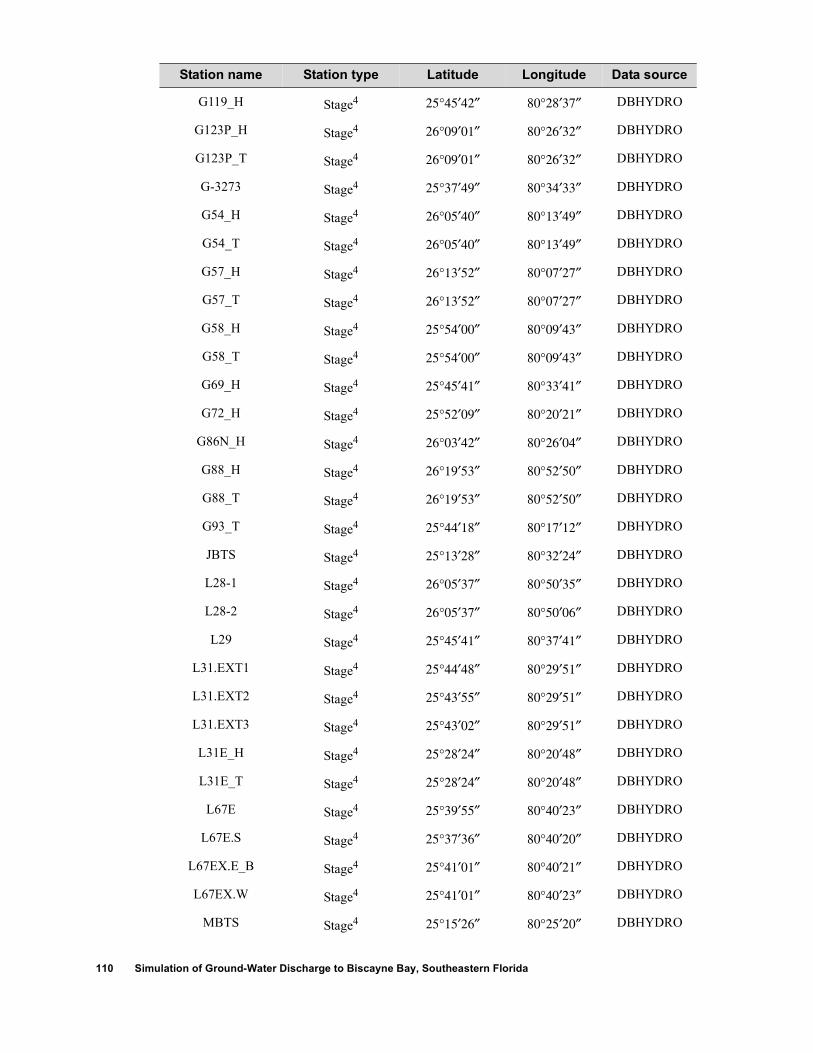
110 Simulation of Ground-Water Discharge to Biscayne Bay, Southeastern Florida
G119_H Stage4 25°45′42″ 80°28′37″ DBHYDRO
G123P_H Stage4 26°09′01″ 80°26′32″ DBHYDRO
G123P_T Stage4 26°09′01″ 80°26′32″ DBHYDRO
G-3273 Stage4 25°37′49″ 80°34′33″ DBHYDRO
G54_H Stage4 26°05′40″ 80°13′49″ DBHYDRO
G54_T Stage4 26°05′40″ 80°13′49″ DBHYDRO
G57_H Stage4 26°13′52″ 80°07′27″ DBHYDRO
G57_T Stage4 26°13′52″ 80°07′27″ DBHYDRO
G58_H Stage4 25°54′00″ 80°09′43″ DBHYDRO
G58_T Stage4 25°54′00″ 80°09′43″ DBHYDRO
G69_H Stage4 25°45′41″ 80°33′41″ DBHYDRO
G72_H Stage4 25°52′09″ 80°20′21″ DBHYDRO
G86N_H Stage4 26°03′42″ 80°26′04″ DBHYDRO
G88_H Stage4 26°19′53″ 80°52′50″ DBHYDRO
G88_T Stage4 26°19′53″ 80°52′50″ DBHYDRO
G93_T Stage4 25°44′18″ 80°17′12″ DBHYDRO
JBTS Stage4 25°13′28″ 80°32′24″ DBHYDRO
L28-1 Stage4 26°05′37″ 80°50′35″ DBHYDRO
L28-2 Stage4 26°05′37″ 80°50′06″ DBHYDRO
L29 Stage4 25°45′41″ 80°37′41″ DBHYDRO
L31.EXT1 Stage4 25°44′48″ 80°29′51″ DBHYDRO
L31.EXT2 Stage4 25°43′55″ 80°29′51″ DBHYDRO
L31.EXT3 Stage4 25°43′02″ 80°29′51″ DBHYDRO
L31E_H Stage4 25°28′24″ 80°20′48″ DBHYDRO
L31E_T Stage4 25°28′24″ 80°20′48″ DBHYDRO
L67E Stage4 25°39′55″ 80°40′23″ DBHYDRO
L67E.S Stage4 25°37′36″ 80°40′20″ DBHYDRO
L67EX.E_B Stage4 25°41′01″ 80°40′21″ DBHYDRO
L67EX.W Stage4 25°41′01″ 80°40′23″ DBHYDRO
MBTS Stage4 25°15′26″ 80°25′20″ DBHYDRO
Station name Station type Latitude Longitude Data source

Appendix III 111
MDTS Stage4 25°16′43″ 80°23′42″ DBHYDRO
MOWRY C Stage4 25°28′14″ 80°20′46″ DBHYDRO
MUD CRK_B Stage4 25°12′14″ 80°35′06″ DBHYDRO
NESRS1 Stage4 25°41′51″ 80°38′04″ DBHYDRO
NESRS2 Stage4 25°43′26″ 80°33′24″ DBHYDRO
NP-112 Stage4 25°25′24″ 80°35′54″ DBHYDRO
NP-127 Stage4 25°21′16″ 80°36′22″ DBHYDRO
NP-146 Stage4 25°15′19″ 80°40′00″ DBHYDRO
NP-158 Stage4 25°23′46″ 80°34′40″ DBHYDRO
NP-203 Stage4 25°37′26″ 80°44′21″ DBHYDRO
NP-311 Stage4 25°26′51″ 80°37′34″ DBHYDRO
NP-31W Stage4 25°26′19″ 80°35′23″ DBHYDRO
NP-A13 Stage4 25°29′56″ 80°42′45″ DBHYDRO
NP-C27 Stage4 25°18′09″ 80°29′19″ DBHYDRO
NP-C50 Stage4 25°18′51″ 80°31′16″ DBHYDRO
NP-CR2 Stage4 25°30′00″ 80°37′18″ DBHYDRO
NP-CR3 Stage4 25°29′54″ 80°39′46″ DBHYDRO
NP-CT3R Stage4 25°17′26″ 80°27′16″ DBHYDRO
NP-CV1S Stage4 25°17′29″ 80°27′15″ DBHYDRO
NP-CV5N Stage4 25°18′14″ 80°29′16″ DBHYDRO
NP-CV5S Stage4 25°18′12″ 80°29′14″ DBHYDRO
NP-CV9N Stage4 25°18′55″ 80°31′15″ DBHYDRO
NP-CV9S Stage4 25°18′54″ 80°31′15″ DBHYDRO
NP-CY2 Stage4 25°19′45″ 80°40′58″ DBHYDRO
NP-CY3 Stage4 25°19′46″ 80°45′02″ DBHYDRO
NP-DO1 Stage4 25°22′25″ 80°41′27″ DBHYDRO
NP-DO2 Stage4 25°23′24″ 80°44′39″ DBHYDRO
NP-EP12R Stage4 25°16′27″ 80°26′42″ DBHYDRO
NP-EP9R Stage4 25°16′20″ 80°33′15″ DBHYDRO
NP-EPG Stage4 25°16′49″ 80°30′11″ DBHYDRO
Station name Station type Latitude Longitude Data source

112 Simulation of Ground-Water Discharge to Biscayne Bay, Southeastern Florida
NP-EPS Stage4 25°16′49″ 80°30′11″ DBHYDRO
NP-EV6 Stage4 25°17′54″ 80°30′42″ DBHYDRO
NP-EV7 Stage4 25°18′36″ 80°32′33″ DBHYDRO
NP-EV8 Stage4 25°20′47″ 80°28′43″ DBHYDRO
NP-N10 Stage4 25°27′43″ 80°36′18″ DBHYDRO
NP-N14 Stage4 25°25′04″ 80°38′20″ DBHYDRO
NP-NMP Stage4 25°15′14″ 80°47′54″ DBHYDRO
NP-NTS1 Stage4 25°26′17″ 80°35′34″ DBHYDRO
NP-NTS3 Stage4 25°26′17″ 80°35′59″ DBHYDRO
NP-P33 Stage4 25°36′31″ 80°41′29″ DBHYDRO
NP-P35 Stage4 25°27′40″ 80°51′52″ DBHYDRO
NP-P36 Stage4 25°31′43″ 80°47′44″ DBHYDRO
NP-P37 Stage4 25°17′09″ 80°41′18″ DBHYDRO
NP-P38 Stage4 25°22′15″ 80°50′00″ DBHYDRO
NP-P44 Stage4 25°25′54″ 80°43′17″ DBHYDRO
NP-P46 Stage4 25°19′11″ 80°47′45″ DBHYDRO
NP-P62 Stage4 25°26′23″ 80°46′58″ DBHYDRO
NP-P67 Stage4 25°19′51″ 80°39′01″ DBHYDRO
NP-P72 Stage4 25°23′46″ 80°42′11″ DBHYDRO
NP-RG1 Stage4 25°34′58″ 80°36′28″ DBHYDRO
NP-RG2 Stage4 25°32′39″ 80°36′21″ DBHYDRO
NP-ROB Stage4 25°26′27″ 80°33′07″ DBHYDRO
NP-SP1 Stage4 25°23′25″ 80°47′50″ DBHYDRO
NP-TMC Stage4 25°36′56″ 80°52′20″ DBHYDRO
NP-TSB Stage4 25°24′06″ 80°36′24″ DBHYDRO
NP-TSH Stage4 25°18′45″ 80°37′50″ DBHYDRO
POND AP1 Stage4 26°04′39″ 80°11′34″ DBHYDRO
POND APP Stage4 26°04′58″ 80°11′41″ DBHYDRO
S11A_H Stage4 26°10′37″ 80°26′55″ DBHYDRO
S11A_T Stage4 26°10′37″ 80°26′55″ DBHYDRO
Station name Station type Latitude Longitude Data source

Appendix III 113
S11B_H Stage4 26°12′09″ 80°27′15″ DBHYDRO
S11B_T Stage4 26°12′09″ 80°27′15″ DBHYDRO
S11C_H Stage4 26°13′46″ 80°27′36″ DBHYDRO
S11C_T Stage4 26°13′46″ 80°27′36″ DBHYDRO
S12_H Stage4 25°45′43″ 80°43′33″ DBHYDRO
S120_H Stage4 25°40′15″ 80°19′17″ DBHYDRO
S121_H Stage4 25°41′13″ 80°21′39″ DBHYDRO
S121_T Stage4 25°41′13″ 80°21′39″ DBHYDRO
S123_T Stage4 25°36′37″ 80°18′28″ DBHYDRO
S124_H Stage4 26°07′45″ 80°21′56″ DBHYDRO
S124_T Stage4 26°07′45″ 80°21′56″ DBHYDRO
S125_H Stage4 26°09′51″ 80°17′51″ DBHYDRO
S125_T Stage4 26°09′51″ 80°17′51″ DBHYDRO
S12A_H Stage4 25°45′42″ 80°49′17″ DBHYDRO
S12A_T Stage4 25°45′42″ 80°49′17″ DBHYDRO
S12B_H Stage4 25°45′42″ 80°46′11″ DBHYDRO
S12B_T Stage4 25°45′42″ 80°46′11″ DBHYDRO
S12C_T Stage4 25°45′43″ 80°43′37″ DBHYDRO
S12D_H Stage4 25°45′44″ 80°40′53″ DBHYDRO
S12D_T Stage4 25°45′44″ 80°40′53″ DBHYDRO
S13_H Stage4 26°03′58″ 80°12′31″ DBHYDRO
S13_T Stage4 26°03′58″ 80°12′31″ DBHYDRO
S13A_H Stage4 26°03′53″ 80°16′49″ DBHYDRO
S13A_T Stage4 26°03′53″ 80°16′49″ DBHYDRO
S13P_H Stage4 26°04′25″ 80°12′37″ DBHYDRO
S13P_T Stage4 26°04′25″ 80°12′37″ DBHYDRO
S140 SPW_H Stage4 26°10′19″ 80°49′38″ DBHYDRO
S140 SPW_T Stage4 26°10′19″ 80°49′38″ DBHYDRO
S140_H Stage4 26°10′19″ 80°49′38″ DBHYDRO
S140_T Stage4 26°10′19″ 80°49′38″ DBHYDRO
Station name Station type Latitude Longitude Data source

114 Simulation of Ground-Water Discharge to Biscayne Bay, Southeastern Florida
S142_H Stage4 26°09′36″ 80°26′46″ DBHYDRO
S142_T Stage4 26°09′36″ 80°26′46″ DBHYDRO
S143_T Stage4 26°10′34″ 80°26′51″ DBHYDRO
S144_H Stage4 26°13′05″ 80°23′52″ DBHYDRO
S144_T Stage4 26°13′05″ 80°23′52″ DBHYDRO
S145_H Stage4 26°13′18″ 80°21′57″ DBHYDRO
S145_T Stage4 26°13′18″ 80°21′57″ DBHYDRO
S146_H Stage4 26°13′31″ 80°20′00″ DBHYDRO
S146_T Stage4 26°13′31″ 80°20′00″ DBHYDRO
S148_T Stage4 25°34′12″ 80°22′58″ DBHYDRO
S166_H Stage4 25°31′06″ 80°25′56″ DBHYDRO
S174_T Stage4 25°29′01″ 80°33′48″ DBHYDRO
S175_H Stage4 25°25′04″ 80°34′25″ DBHYDRO
S20_H Stage4 25°22′01″ 80°22′35″ DBHYDRO
S20_T Stage4 25°22′01″ 80°22′35″ DBHYDRO
S20G_T Stage4 25°29′21″ 80°20′50″ DBHYDRO
S21_T Stage4 25°32′35″ 80°19′51″ DBHYDRO
S22_T Stage4 25°40′12″ 80°17′02″ DBHYDRO
S27_T Stage4 25°50′55″ 80°11′20″ DBHYDRO
S28_H Stage4 25°52′15″ 80°10′42″ DBHYDRO
S28_T Stage4 25°52′15″ 80°10′42″ DBHYDRO
S29_T Stage4 25°55′42″ 80°09′03″ DBHYDRO
S30_H Stage4 25°57′24″ 80°25′53″ DBHYDRO
S32_H Stage4 25°56′33″ 80°26′22″ DBHYDRO
S33_H Stage4 26°08′08″ 80°11′27″ DBHYDRO
S33_T Stage4 26°08′08″ 80°11′27″ DBHYDRO
S332 Stage4 25°25′18″ 80°35′23″ DBHYDRO
S334_T Stage4 25°45′42″ 80°30′08″ DBHYDRO
S335_T Stage4 25°46′34″ 80°28′58″ DBHYDRO
S336_T Stage4 25°45′41″ 80°29′48″ DBHYDRO
Station name Station type Latitude Longitude Data source

Appendix III 115
S337_H Stage4 25°56′32″ 80°26′27″ DBHYDRO
S339_H Stage4 26°13′03″ 80°41′25″ DBHYDRO
S339_T Stage4 26°13′03″ 80°41′25″ DBHYDRO
S34_H Stage4 26°09′01″ 80°26′32″ DBHYDRO
S34_T Stage4 26°09′01″ 80°26′32″ DBHYDRO
S340_H Stage4 26°07′07″ 80°36′44″ DBHYDRO
S343A_H Stage4 25°47′20″ 80°51′19″ DBHYDRO
S343A_T Stage4 25°47′20″ 80°51′19″ DBHYDRO
S343B_H Stage4 25°46′41″ 80°50′39″ DBHYDRO
S343B_T Stage4 25°46′41″ 80°50′39″ DBHYDRO
S344_H Stage4 25°55′08″ 80°50′11″ DBHYDRO
S344_T Stage4 25°55′08″ 80°50′11″ DBHYDRO
S36_H Stage4 26°10′24″ 80°10′42″ DBHYDRO
S36_T Stage4 26°10′24″ 80°10′42″ DBHYDRO
S37A_H Stage4 26°12′21″ 80°07′56″ DBHYDRO
S37A_T Stage4 26°12′21″ 80°07′56″ DBHYDRO
S37B_H Stage4 26°13′26″ 80°10′15″ DBHYDRO
S37B_T Stage4 26°13′26″ 80°10′15″ DBHYDRO
S38_H Stage4 26°13′47″ 80°17′54″ DBHYDRO
S38_T Stage4 26°13′47″ 80°17′54″ DBHYDRO
S38A_H Stage4 26°13′49″ 80°17′52″ DBHYDRO
S38C_H Stage4 26°13′44″ 80°17′52″ DBHYDRO
S38C_T Stage4 26°13′44″ 80°17′52″ DBHYDRO
S9_H Stage4 26°03′41″ 80°26′29″ DBHYDRO
S9BFN Stage4 26°04′02″ 80°26′24″ DBHYDRO
S9BFS Stage4 26°03′14″ 80°26′23″ DBHYDRO
S9XN_H Stage4 26°03′43″ 80°26′35″ DBHYDRO
SHARK.1_H Stage4 25°47′55″ 80°34′42″ DBHYDRO
SNAPPERN Stage4 25°50′53″ 80°23′02″ DBHYDRO
SWEVER1 Stage4 25°19′47″ 80°25′47″ DBHYDRO
Station name Station type Latitude Longitude Data source

116 Simulation of Ground-Water Discharge to Biscayne Bay, Southeastern Florida
SWEVER2A Stage4 25°19′07″ 80°28′33″ DBHYDRO
SWEVER2B Stage4 25°18′56″ 80°28′33″ DBHYDRO
SWEVER3 Stage4 25°20′44″ 80°39′23″ DBHYDRO
SWEVER4 Stage4 25°20′37″ 80°32′42″ DBHYDRO
SWEVER5A Stage4 25°17′17″ 80°34′20″ DBHYDRO
SWEVER5B Stage4 25°17′25″ 80°34′13″ DBHYDRO
TPTS Stage4 25°12′23″ 80°22′29″ DBHYDRO
TROUT CR_B Stage4 25°12′55″ 80°32′01″ DBHYDRO
G119_T Stage4,5 25°45′42″ 80°28′37″ DBHYDRO
G211_H Stage4,5 25°39′31″ 80°29′52″ DBHYDRO
G211_T Stage4,5 25°39′31″ 80°29′52″ DBHYDRO
G72_T Stage4,5 25°52′09″ 80°20′21″ DBHYDRO
G93_H Stage4,5 25°44′18″ 80°17′12″ DBHYDRO
S118_H Stage4,5 25°37′22″ 80°20′30″ DBHYDRO
S118_T Stage4,5 25°37′22″ 80°20′30″ DBHYDRO
S119_H Stage4,5 25°38′33″ 80°20′18″ DBHYDRO
S119_T Stage4,5 25°38′33″ 80°20′18″ DBHYDRO
S120_T Stage4,5 25°40′15″ 80°19′17″ DBHYDRO
S122_H Stage4,5 25°35′39″ 80°20′53″ DBHYDRO
S122_T Stage4,5 25°35′39″ 80°20′53″ DBHYDRO
S123_H Stage4,5 25°36′37″ 80°18′28″ DBHYDRO
S148_H Stage4,5 25°34′12″ 80°22′58″ DBHYDRO
S149_H Stage4,5 25°35′31″ 80°21′40″ DBHYDRO
S151_H Stage4,5 26°00′43″ 80°30′35″ DBHYDRO
S151_T Stage4,5 26°00′43″ 80°30′35″ DBHYDRO
S165_H Stage4,5 25°32′33″ 80°24′34″ DBHYDRO
S165_T Stage4,5 25°32′33″ 80°24′34″ DBHYDRO
S166_T Stage4,5 25°31′06″ 80°25′56″ DBHYDRO
S167_H Stage4,5 25°30′09″ 80°27′48″ DBHYDRO
S167_T Stage4,5 25°30′09″ 80°27′48″ DBHYDRO
Station name Station type Latitude Longitude Data source

Appendix III 117
S174_H Stage4,5 25°29′01″ 80°33′48″ DBHYDRO
S175_T Stage4,5 25°25′04″ 80°34′25″ DBHYDRO
S176_H Stage4,5 25°28′58″ 80°33′46″ DBHYDRO
S176_T Stage4,5 25°28′58″ 80°33′46″ DBHYDRO
S177_H Stage4,5 25°24′10″ 80°33′30″ DBHYDRO
S177_T Stage4,5 25°24′10″ 80°33′30″ DBHYDRO
S178_H Stage4,5 25°24′29″ 80°31′26″ DBHYDRO
S178_T Stage4,5 25°24′29″ 80°31′26″ DBHYDRO
S179_H Stage4,5 25°28′25″ 80°24′52″ DBHYDRO
S179_T Stage4,5 25°28′25″ 80°24′52″ DBHYDRO
S18C_H Stage4,5 25°19′50″ 80°31′30″ DBHYDRO
S18C_T Stage4,5 25°19′50″ 80°31′30″ DBHYDRO
S194_H Stage4,5 25°34′59″ 80°28′42″ DBHYDRO
S194_T Stage4,5 25°34′59″ 80°28′42″ DBHYDRO
S195_H Stage4,5 25°33′04″ 80°23′46″ DBHYDRO
S195_T Stage4,5 25°33′04″ 80°23′46″ DBHYDRO
S196_H Stage4,5 25°31′01″ 80°30′41″ DBHYDRO
S196_T Stage4,5 25°31′01″ 80°30′41″ DBHYDRO
S197_H Stage4,5 25°17′13″ 80°26′29″ DBHYDRO
S197_T Stage4,5 25°17′13″ 80°26′29″ DBHYDRO
S20F_H Stage4,5 25°27′46″ 80°20′51″ DBHYDRO
S20F_T Stage4,5 25°27′46″ 80°20′51″ DBHYDRO
S20G_H Stage4,5 25°29′21″ 80°20′50″ DBHYDRO
S21_H Stage4,5 25°32′35″ 80°19′51″ DBHYDRO
S21A_H Stage4,5 25°31′09″ 80°20′46″ DBHYDRO
S21A_T Stage4,5 25°31′09″ 80°20′46″ DBHYDRO
S22_H Stage4,5 25°40′12″ 80°17′02″ DBHYDRO
S25_H Stage4,5 25°47′52″ 80°14′44″ DBHYDRO
S25_T Stage4,5 25°47′52″ 80°14′44″ DBHYDRO
S25B_H Stage4,5 25°47′38″ 80°15′45″ DBHYDRO
Station name Station type Latitude Longitude Data source

118 Simulation of Ground-Water Discharge to Biscayne Bay, Southeastern Florida
S25B_T Stage4, 25°47′38″ 80°15′45″ DBHYDRO
S26_H Stage4,5 25°48′29″ 80°15′39″ DBHYDRO
S26_T Stage4,5 25°48′29″ 80°15′39″ DBHYDRO
S27_H Stage4,5 25°50′55″ 80°11′20″ DBHYDRO
S29_H Stage4,5 25°55′42″ 80°09′03″ DBHYDRO
S30_T Stage4,5 25°57′24″ 80°25′53″ DBHYDRO
S31_H Stage4,5 25°56′34″ 80°26′25″ DBHYDRO
S31_T Stage4,5 25°56′34″ 80°26′25″ DBHYDRO
S331_H Stage4,5 25°36′39″ 80°30′35″ DBHYDRO
S331_T Stage4,5 25°36′39″ 80°30′35″ DBHYDRO
S332_H Stage4,5 25°25′18″ 80°35′23″ DBHYDRO
S332_T Stage4,5 25°25′18″ 80°35′23″ DBHYDRO
S333_H Stage4,5 25°45′43″ 80°40′27″ DBHYDRO
S333_T Stage4,5 25°45′43″ 80°40′27″ DBHYDRO
S334_H Stage4,5 25°45′42″ 80°30′08″ DBHYDRO
S335_H Stage4,5 25°46′34″ 80°28′58″ DBHYDRO
S336_H Stage4,5 25°45′41″ 80°29′48″ DBHYDRO
S337_T Stage4,5 25°56′32″ 80°26′27″ DBHYDRO
S338_H Stage4,5 25°39′38″ 80°28′49″ DBHYDRO
S338_T Stage4,5 25°39′38″ 80°28′49″ DBHYDRO
S340_T Stage4,5 26°07′07″ 80°36′44″ DBHYDRO
S9_T Stage4,5 26°03′41″ 80°26′29″ DBHYDRO
G72_C Flow6 25°52′09″ 80°20′21″ DBHYDRO
G93 Flow6 25°44′18″ 80°17′12″ DBHYDRO
S122_C Flow6 25°35′39″ 80°20′53″ DBHYDRO
S123_S Flow6 25°36′37″ 80°18′28″ DBHYDRO
S173_C Flow6 25°36′39″ 80°30′35″ DBHYDRO
S174_S Flow6 25°29′01″ 80°33′48″ DBHYDRO
S194_C Flow6 25°34′59″ 80°28′42″ DBHYDRO
S196_C Flow6 25°31′01″ 80°30′41″ DBHYDRO
Station name Station type Latitude Longitude Data source

Appendix III 119
S196_C Flow6 25°31′01″ 80°30′41″ DBHYDRO
S197_C Flow6 25°17′13″ 80°26′29″ DBHYDRO
S20F_S Flow6 25°27′46″ 80°20′51″ DBHYDRO
S21_S Flow6 25°32′35″ 80°19′51″ DBHYDRO
S21A_S Flow6 25°31′09″ 80°20′46″ DBHYDRO
S22_S Flow6 25°40′12″ 80°17′02″ DBHYDRO
S25_C Flow6 25°47′52″ 80°14′44″ DBHYDRO
S25B_S Flow6 25°47′38″ 80°15′45″ DBHYDRO
S26_S Flow6 25°48′29″ 80°15′39″ DBHYDRO
S27_S Flow6 25°50′55″ 80°11′20″ DBHYDRO
S28_S Flow6 25°52′15″ 80°10′42″ DBHYDRO
S29_S Flow6 25°55′42″ 80°09′03″ DBHYDRO
S31_C Flow6 25°56′34″ 80°26′25″ DBHYDRO
S32_C Flow6 25°56′33″ 80°26′22″ DBHYDRO
S331_P Flow6 25°36′39″ 80°30′35″ DBHYDRO
S338_C Flow6 25°39′38″ 80°28′49″ DBHYDRO
1Used for regional-scale model to calibrate ground-water heads.
2Included in the U.S. Geological Survey saltwater intrusion monitoring network.
3Used for regional-scale model to develop Recharge package.
4Used for regional-scale model to assign stage values for general-head boundaries.
5Used for regional-scale model to assign stage values for River package.
6Used for regional-scale model to calibrate ground-water baseflow to canals.
Station name Station type Latitude Longitude Data source

120 Simulation of Ground-Water Discharge to Biscayne Bay, Southeastern Florida

Appendix IV 121
Appendix IVVerification of the SEAWAT Code
The SEAWAT code is relatively new and has not been widely used and tested. For this reason and because the code was modified for this study, SEAWAT was verified by running four different prob-lems and comparing the results to those from other variable-density codes. Voss and Souza (1987) suggest that new variable-density codes should be tested and verified by running four or five benchmark problems that vary in complexity. These benchmark problems are listed below with the reference that describes the problem:ï Box problems (Voss and Souza, 1987)ï Henry problem (Voss and Souza, 1987)ï Elder problem (Voss and Souza, 1987)ï HYDROCOIN problem (Konikow and others, 1997)
ï Salt-lake problem (Simmons and others, 1999)
This appendix presents the development and results for four of the benchmark problems listed above. The salt-lake problem has not yet been simulated with SEAWAT.
For each of the four problems evaluated, the results from SEAWAT compare reasonably well with the results from other numerical codes. From these comparisons, SEAWAT was determined to be an acceptable code for simulating the variable-density component of ground-water flow. As discussed in the report, the SEAWAT code was also modified to include variable-density sources and sinks. These additional features seem to work properly in the code, but they have not yet been verified against the results from other codes because benchmark problems for these types of features do not currently exist.
Box Problems
The purpose of the box problems is to verify that fluid velocities are properly calculated by the simulation code. Although inconsistent approxima-tions for velocity are more likely to occur with finite-element models, the box problems also provide a good test for variable-density codes based on the finite-difference approximation. There are two different cases of the box problem (Voss and Souza, 1987). In the first case, the variable-density code is tested by simulating flow within a two-dimensional, vertical cross-sectional model with no-flow boundaries on all sides. The size of the model domain and values for hydraulic conductivity and porosity are not important. Dispersivity values should be set to a length similar in size to the length of a model cell, and the diffusion coefficient should be set to zero. The initial conditions within the box consist of a layer of freshwater overly-ing a layer of saltwater−a stable configuration for fluid density. When this model is run with steady-state con-ditions, the interface between freshwater and saltwater should remain in the same layer of the model.
For the second case of the box problem, the ini-tial condition and dispersion parameters are the same as the first case, but horizontal flow is induced across the box by setting different hydrostatic pressure boundaries on the left and right sides of the model. If the code is programmed correctly, the interface between freshwater and saltwater should remain in the same layer of the model.
SEAWAT was tested with both cases of the box problem. In each case, the interface remained in the correct model layer. This indicates that the velocity approximation used by SEAWAT is probably valid.

122 Simulation of Ground-Water Discharge to Biscayne Bay, Southeastern Florida
Henry Problem
Henry (1964) presented an analytical solution for a problem that is thought to represent fresh ground water flowing toward a seawater boundary. Because an analytical solution was available for the Henry problem, many numerical codes were evaluated and tested with the Henry solution. Segol (1993) showed, however, that the Henry solution was not exact because Henry (1964) eliminated, for computational reasons, mathematical terms from the solution that were thought to be insignificant. When Segol (1993) recalculated Henryís solution with the additional terms, the improved answer was slightly different from the original solution. With the new solution, Segol (1993) showed that numerical codes such as SUTRA (Voss, 1984) could reproduce the correct answer for the Henry problem.
The basic design of the Henry problem is shown in figure A1. The cross-sectional box is 2 m long by 1 m high by 1 m wide. A constant flux of fresh ground water is applied to the left boundary at a rate (Qin) of 5.702 m3/d per meter with a concentration (Cin) equal to zero. A constant-head boundary is applied to the right side of the box to represent seawater hydrostatic conditions. The head value applied to the constant head cells is set equal to 1 m and then converted to freshwater head values that increase appropriately with depth. The upper and lower model boundaries represent no flow.
The Henry problem caused further confusion among the modeling community because researchers attempting to verify numerical codes calculated an erroneous value for molecular diffusion that did not correlate with the original value used by Henry (Voss and Souza, 1987). For this reason, some researchers consider there to be two cases of the Henry problem: one in which the value for molecular diffusion (Dm) is 0.57024 m2/d and another with a Dm value of 1.62925 m2/d (fig. A2).
The finite-difference model grid used to dis-cretize the problem domain consists of 21 columns and 10 layers. Each cell, with the exception of the cells in column 21, is 0.1 by 0.1 m in size. Cells in column 21 are 0.01-m horizontal by 0.1-m vertical. The nar-row column of cells at the right side of the model was used to more precisely locate the seawater hydrostatic boundary at a distance of 2 meters.
The comparison between SEAWAT and SUTRA results (Segol, 1993) for the Henry problem are shown in figure A2. Contours of relative salinity are in good agreement for both cases, especially away from the right boundary. Discrepancies in contours of relative salinity between the two models at the right boundary are probably due to differences in the way finite-element and finite-difference models locate and represent constant-head (or pressure) boundaries.
Elder Problem
The Elder problem was originally designed for heat flow (Elder, 1967), but Voss and Souza (1987) recast the problem as a variable-density ground-water problem in which fluid density is a function of salt concentration. The Elder problem is commonly used to verify variable-density ground-water codes. The geometry and boundary conditions for the problem are shown in figure A3. A constant-concentration boundary is specified for part of the upper boundary. During the simulation, salt from the constant-concentration boundary dif-fuses into the model domain and initiates complex vortices that redistribute salt mass throughout the model. A constant-concentration boundary with a value of zero is specified for the lowest layer in the model. Two outlet cells with constant-head values of zero are specified for the upper left and right boundaries. These constant-head cells allow salt to diffuse into the model by providing an outlet for fluid and salt mass.
The Elder problem was run with the SEAWAT code for a period of 20 years. Several different methods were used to solve the transport equation. The MOC and the implicit solver with a central-in-space weighting scheme provided solu-tions closest to those of SUTRA (Voss and Souza, 1987) and those of Elder (1967). Relative concen-trations from SEAWAT are compared with results from SUTRA (Voss and Souza, 1987) and the orig-inal nondimensional results from Elder (1967) for six different times (fig. A4). For each time, there seems to be a good match between the results from SEAWAT and SUTRA (Voss and Souza, 1987) and those of Elder (1967).

Appendix IV 123
HYDROCOIN Problem
The purpose of the Hydrologic Code Intercom-parison project (HYDROCOIN) was to evaluate the accuracy of selected ground-water modeling codes. One of the problems used for testing is referred to as the HYDROCOIN problem. The HYDROCOIN prob-lem presented here is based on case 5 that was reevalu-ated by Konikow and others (1997). The general geometry and boundary conditions for the problem are shown in figure A5. A sloping pressure boundary is imposed across the top of the box that is surrounded on the sides and bottom by no-flow conditions. Along the base of the middle portion of the model, a constant concentration condition is applied to represent the top of a salt dome. As ground water flows along the
bottom boundary, salt disperses into the system and collects in the lower right corner of the model domain.
The SEAWAT code was used to simulate the HYDROCOIN problem and uses the general design employed by Konikow and others (1997). Prior to sim-ulating the HYDROCOIN problem, the SEAWAT code was slightly modified to use the equation of state for fluid density as used by Konikow and others (1997). The comparison between SEAWAT and MOCDENSE is shown in figure A6. In general, the relative concentrations simulated by the two codes are consistent with one another. There is a discrepancy toward the upper right part of the model domain. While SEAWAT tends to produce slightly higher concentrations in this region, the comparison between the two codes is considered acceptable.
Qin
,C
in
1.0 METER
SE
AW
AT
ER
HY
DR
OS
TA
TIC
= 0.35
= 35 kilograms per cubic meter
= 1,025 kilograms per cubic meter
=25
35
= 1,000 kilograms per cubic meter
= 5.702 cubic meters per day per meter
= 864 meters per day
=T
= 0.0
= 0.57024 square meter per day (Case 1)
= 1.62925 square meters per day (Case 2)
�
1.00
0
2.0
DISTANCE, IN METERS
n
Cs
s
C
f
QinKf
L
DmDm
���
�
�
�
Figure A1. Boundary conditions and model parameters for the Henry problem.

124 Simulation of Ground-Water Discharge to Biscayne Bay, Southeastern Florida
SEAWAT
SUTRA (Segol, 1993)
0 0.2 0.4 0.6 0.8 1.2 1.4 1.6 1.80
0.2
0.4
0.6
0.8
0 0.2 0.4 0.6 0.8 1.2 1.4 1.6 1.80
0.2
0.4
0.6
0.8
1
5
10
25
50 75 90
95
DISTANCE, IN METERS
DISTANCE, IN METERS
ELE
VA
TIO
N,IN
ME
TE
RS
ELE
VA
TIO
N,IN
ME
TE
RS
Dm = 1.62925 SQUARE METERS PER DAY
Dm = 0.57024 SQUARE METER PER DAY
0 0.2 0.4 0.6 0.8 1.2 1.4 1.6 1.80
0.2
0.4
0.6
0.8
0 0.2 0.4 0.6 0.8 1.0
1.0
1.2 1.4 1.6 1.8 2.0
2.0
0
0.2
0.4
0.6
0.8
1.0
1.0
1
10
25
50
75
90
9599
5
EXPLANATION
Relative concentration,in percent
Figure A2. Comparison between SEAWAT and SUTRA for the Henry problem.

Appendix IV 125
P = 0 P = 0
Cs = 285.7
C = 0.0
n = 0.10
K
= 1,200 kilograms per cubic meter
=25
35
D
f
s
f
m
L
= 0.411 meter per day
= 1,000 kilograms per cubic meter
C
= 0.308 square meter per day
= = 0.0
��
�
���
�T
300 METERS
600 METERS
150
ME
TE
RS
Figure A3. Boundary conditions and model parameters for the Elder problem.

126 Simulation of Ground-Water Discharge to Biscayne Bay, Southeastern Florida
1 year 10 years
2 years 15 years
3 years 20 years
SEAWAT
SUTRA (Voss and Souza, 1987)
Elder (1967)
EXPLANATION
20
20
20
20
20
20
60
60
60
60
60
Relative concentration,in percent
Figure A4. Comparison between SEAWAT, SUTRA and Elderís solution for the Elder problem.

Appendix IV 127
Salt dome
� = 1,000 kilograms per cubic meters
( = 1,200 kilograms per cubic meter, Cs = 1.0)�
1=
C
s+
(1-C)
f� � �
= 0.8476 meter per day
= 1,000 kilograms per cubic meter
= 20 meters
= 2 meters
= 0.0
= 0.2
= 1,200 kilograms per cubic meter
0D
EP
TH
,IN
ME
TE
RS
DISTANCE, IN METERS
0
300
900
SLOPING PRESSURE BOUNDARY
Kfn
f
L
T
Dm
s
����
Figure A5. Boundary conditions and model parameters for the HYDROCOIN problem (from Konikow and others, 1997).
SEAWAT
MOCDENSE (Konikow and others, 1997)
DISTANCE, IN METERS
ELE
VA
TIO
N,IN
ME
TE
RS
EXPLANATION
Relative concentration
-100
0
-200
-3000 100 200 300 400 500 600 700 800 900
0.05
0.10
0.20
0.30
Figure A6. Comparison between SEAWAT and MOCDENSE for the HYDROCOIN problem.

U.S. ARMY CORPS OF ENGINEERS
PREPARED AS PART OF THE U.S. GEOLOGICAL SURVEYPLACE-BASED STUDIES PROGRAM IN COOPERATION WITH THE
Langevin, C.D., 2001, Simulation of ground-water discharge to Biscayne Bay, southeastern Florida
PLATE 1. SECTIONS SHOWING SENSITIVITY ANALYSIS RESULTS FOR THE COCONUT GROVE MODEL
ByChristian D. Langevin
2001
U.S. DEPARTMENT OF THE INTERIORU.S. GEOLOGICAL SURVEY
WATER-RESOURCES INVESTIGATIONS REPORT 00-4251Sections showing sensitivity analysis results for the Coconut Grove model–PLATE 1
Biscayne Bay
Biscayne Bay Biscayne Bay
Biscayne Bay Biscayne Bay
Biscayne Bay Biscayne Bay
Biscayne Bay Biscayne Bay
Biscayne Bay
Biscayne Bay
Biscayne Bay
-5,500 -5,000 -4,500 -4,000 -3,500 -3,000 -2,500 -2,000 -1,500 -1,000 -500 0 500 1,000 1,500 2,000-5,500 -5,000 -4,500 -4,000 -3,500 -3,000 -2,500 -2,000 -1,500 -1,000 -500 0 500 1,000 1,500 2,000
Base case: line on upper graphs represents simulated head; lines oncontour plot represent salinity concentration relative to seawater
Sensitivity run: line on upper graphs represents simulated head; lines oncontour plot represent salinity concentration relative to seawater
Interface between freshwater and saltwater calculated with the Ghyben-Herzberg relation and the simulated heads from the sensitivity run
Horizontal hydraulic conductivity, as equivalent freshwater term
Vertical hydraulic conductivity, as equivalent freshwater term
Longitudinal dispersivity
Transverse dispersivity
Constant flux value for flow into model at western boundary
Recharge
EXPLANATION
KV
�L
�T
Q/m
R
Kh
K = 18,000 meters per dayh
HE
AD
,IN
ME
TE
RS 1.5
1.0
0.5
0
K = 4,500 meters per dayh
EL
EV
AT
ION
,IN
ME
TE
RS
HE
AD
,IN
ME
TE
RS 1.5
1.0
0.5
0
-10
-20
-30
K = 0.9 meter per dayv
�L = 10 meters
DISTANCE FROM SHORE, IN METERS
�L = 0.1 meter
�T = 0.2 meter�T = 0.05 meter
Q/m = 30 square meters per dayQ/m = 7.5 square meters per day
K = 90 meters per dayv
R = 76 centimeters per yearR = 19 centimeters per year
Salinity concentration of sensitivity run, relative to seawater
Base case, K = 9,000 meters per dayh
Base case, K = 9 meters per dayV
Base case, = 1 meter�L
Base case, = 0.1 meter�T
DISTANCE FROM SHORE, IN METERS
DISTANCE FROM SHORE, IN METERS
DISTANCE FROM SHORE, IN METERS
Base case, Q/m = 15 square meters per day
DISTANCE FROM SHORE, IN METERS
Base case, R = 38 centimeters per year
DISTANCE FROM SHORE, IN METERS
DISTANCE FROM SHORE, IN METERS
DISTANCE FROM SHORE, IN METERS
DISTANCE FROM SHORE, IN METERS
DISTANCE FROM SHORE, IN METERS
DISTANCE FROM SHORE, IN METERS
DISTANCE FROM SHORE, IN METERS
EL
EV
AT
ION
,IN
ME
TE
RS
HE
AD
,IN
ME
TE
RS 1.5
1.0
0.5
0
EL
EV
AT
ION
,IN
ME
TE
RS
HE
AD
,IN
ME
TE
RS 1.5
1.0
0.5
0
EL
EV
AT
ION
,IN
ME
TE
RS
HE
AD
,IN
ME
TE
RS 1.5
1.0
0.5
0
EL
EV
AT
ION
,IN
ME
TE
RS
HE
AD
,IN
ME
TE
RS 1.5
1.0
0.5
0
EL
EV
AT
ION
,IN
ME
TE
RS
HE
AD
,IN
ME
TE
RS 1.5
1.0
0.5
0
EL
EV
AT
ION
,IN
ME
TE
RS
HE
AD
,IN
ME
TE
RS 1.5
1.0
0.5
0
EL
EV
AT
ION
,IN
ME
TE
RS
HE
AD
,IN
ME
TE
RS 1.5
1.0
0.5
0
EL
EV
AT
ION
,IN
ME
TE
RS
HE
AD
,IN
ME
TE
RS 1.5
1.0
0.5
0
EL
EV
AT
ION
,IN
ME
TE
RS
HE
AD
,IN
ME
TE
RS 1.5
1.0
0.5
0
EL
EV
AT
ION
,IN
ME
TE
RS
HE
AD
,IN
ME
TE
RS 1.5
1.0
0.5
0
EL
EV
AT
ION
,IN
ME
TE
RS
0.05 0.50 0.95
-5,500 -5,000 -4,500 -4,000 -3,500 -3,000 -2,500 -2,000 -1,500 -1,000 -500 0 500 1,000 1,500 2,000
-5,500 -5,000 -4,500 -4,000 -3,500 -3,000 -2,500 -2,000 -1,500 -1,000 -500 0 500 1,000 1,500 2,000
-5,500 -5,000 -4,500 -4,000 -3,500 -3,000 -2,500 -2,000 -1,500 -1,000 -500 0 500 1,000 1,500 2,000
-5,500 -5,000 -4,500 -4,000 -3,500 -3,000 -2,500 -2,000 -1,500 -1,000 -500 0 500 1,000 1,500 2,000
-5,500 -5,000 -4,500 -4,000 -3,500 -3,000 -2,500 -2,000 -1,500 -1,000 -500 0 500 1,000 1,500 2,000
-5,500 -5,000 -4,500 -4,000 -3,500 -3,000 -2,500 -2,000 -1,500 -1,000 -500 0 500 1,000 1,500 2,000
-5,500 -5,000 -4,500 -4,000 -3,500 -3,000 -2,500 -2,000 -1,500 -1,000 -500 0 500 1,000 1,500 2,000
-5,500 -5,000 -4,500 -4,000 -3,500 -3,000 -2,500 -2,000 -1,500 -1,000 -500 0 500 1,000 1,500 2,000
-5,500 -5,000 -4,500 -4,000 -3,500 -3,000 -2,500 -2,000 -1,500 -1,000 -500 0 500 1,000 1,500 2,000
-5,500 -5,000 -4,500 -4,000 -3,500 -3,000 -2,500 -2,000 -1,500 -1,000 -500 0 500 1,000 1,500 2,000
-10
-20
-30
-10
-20
-30
-10
-20
-30
-10
-20
-30
-10
-20
-30
-10
-20
-30
-10
-20
-30
-10
-20
-30
-10
-20
-30
-10
-20
-30
-10
-20
-30

U.S. ARMY CORPS OF ENGINEERS
PREPARED AS PART OF THE U.S. GEOLOGICAL SURVEYPLACE-BASED STUDIES PROGRAM IN COOPERATION WITH THE
Langevin, C.D., 2001, Simulation of ground-water discharge to Biscayne Bay, southeastern Florida
PLATE 2. SECTIONS SHOWING SENSITIVITY ANALYSIS RESULTS FOR THE DEERING ESTATE MODEL
ByChristian D. Langevin
2001
U.S. DEPARTMENT OF THE INTERIORU.S. GEOLOGICAL SURVEY
WATER-RESOURCES INVESTIGATIONS REPORT 00-4251Sections showing sensitivity analysis results for the Deering Estate model–PLATE 2
Base case: line on upper graphs represents simulated head; lines oncontour plot represent salinity concentration relative to seawater
Sensitivity run: line on upper graphs represents simulated head; lines oncontour plot represent salinity concentration relative to seawater
Interface between freshwater and saltwater calculated with the Ghyben-Herzberg relation and the simulated heads from the sensitivity run
Horizontal hydraulic conductivity, as equivalent freshwater term
Vertical hydraulic conductivity, as equivalent freshwater term
Longitudinal dispersivity
Transverse dispersivity
Constant flux value for flow into model at western boundary
Recharge
EXPLANATION
KV
�L
�T
Q/m
R
Kh
K = 2,000 meters per dayh
HE
AD
,IN
ME
TE
RS 1.5
1.0
0.5
0
Biscayne Bay
-700 -600 -500 -400 -300 -200 -100 0 100 200 300
K = 500 meters per dayh
EL
EV
AT
ION
,IN
ME
TE
RS
HE
AD
,IN
ME
TE
RS 1.5
1.0
0.5
0
-10
-20
-30
Biscayne Bay
-700 -600 -500 -400 -300 -200 -100 0 100 200 300
K = 50 meters per dayv
Biscayne Bay
-700 -600 -500 -400 -300 -200 -100 0 100 200 300
�L = 20 meters
Biscayne Bay
-700 -600 -500 -400 -300 -200 -100 0 100 200 300
DISTANCE FROM SHORE, IN METERS
�L = 5 meters
Biscayne Bay
-700 -600 -500 -400 -300 -200 -100 0 100 200 300
�T = 2 meters
Biscayne Bay
-700 -600 -500 -400 -300 -200 -100 0 100 200 300
�T = 0.5 meter
Biscayne Bay
-700 -600 -500 -400 -300 -200 -100 0 100 200 300
Q/m coastline = 10 square meters per day
Biscayne Bay
-700 -600 -500 -400 -300 -200 -100 0 100 200 300
Q/m coastline = 2.5 square meters per day
Biscayne Bay
-700 -600 -500 -400 -300 -200 -100 0 100 200 300
K = 200 meters per dayv
Biscayne Bay
-700 -600 -500 -400 -300 -200 -100 0 100 200 300
R = 76 centimeters per year
Biscayne Bay
-700 -600 -500 -400 -300 -200 -100 0 100 200 300
R = 19 centimeters per year
Biscayne Bay
-700 -600 -500 -400 -300 -200 -100 0 100 200 300
Salinity concentration of sensitivity run, relative to seawater
Base case, K = 1,000 meters per dayh
Base case, K = 100 meters per dayV
Base case, = 10 meters�L
Base case, = 1 meter�T
DISTANCE FROM SHORE, IN METERS
DISTANCE FROM SHORE, IN METERS
DISTANCE FROM SHORE, IN METERS
Base case, Q/m = 5 square meters per day
DISTANCE FROM SHORE, IN METERS
Base case, R = 37 centimeters per year
DISTANCE FROM SHORE, IN METERS
DISTANCE FROM SHORE, IN METERS
DISTANCE FROM SHORE, IN METERS
DISTANCE FROM SHORE, IN METERS
DISTANCE FROM SHORE, IN METERS
DISTANCE FROM SHORE, IN METERS
DISTANCE FROM SHORE, IN METERS
EL
EV
AT
ION
,IN
ME
TE
RS
-10
-20
-30
HE
AD
,IN
ME
TE
RS 1.5
1.0
0.5
0
EL
EV
AT
ION
,IN
ME
TE
RS
-10
-20
-30
HE
AD
,IN
ME
TE
RS 1.5
1.0
0.5
0
EL
EV
AT
ION
,IN
ME
TE
RS
-10
-20
-30
HE
AD
,IN
ME
TE
RS 1.5
1.0
0.5
0
EL
EV
AT
ION
,IN
ME
TE
RS
-10
-20
-30
HE
AD
,IN
ME
TE
RS 1.5
1.0
0.5
0
EL
EV
AT
ION
,IN
ME
TE
RS
-10
-20
-30
HE
AD
,IN
ME
TE
RS 1.5
1.0
0.5
0
EL
EV
AT
ION
,IN
ME
TE
RS
-10
-20
-30
HE
AD
,IN
ME
TE
RS 1.5
1.0
0.5
0
EL
EV
AT
ION
,IN
ME
TE
RS
-10
-20
-30
HE
AD
,IN
ME
TE
RS 1.5
1.0
0.5
0
EL
EV
AT
ION
,IN
ME
TE
RS
-10
-20
-30
HE
AD
,IN
ME
TE
RS 1.5
1.0
0.5
0
EL
EV
AT
ION
,IN
ME
TE
RS
-10
-20
-30
HE
AD
,IN
ME
TE
RS 1.5
1.0
0.5
0
EL
EV
AT
ION
,IN
ME
TE
RS
-10
-20
-30
HE
AD
,IN
ME
TE
RS 1.5
1.0
0.5
0
EL
EV
AT
ION
,IN
ME
TE
RS
-10
-20
-30
0.05 0.50 0.95

213
ATLANTICOCEAN
BiscayneBay
��
��
��
��
��
��
��
��
��
�
��
��
�
��
��
�
��
��
�
��
��
Flo
rida
Bay
COLLIERCOUNTY
MIAMI-DADECOUNTY
BR
OW
AR
DC
OU
NT
Y
MIA
MI-
DA
DE
CO
UN
TY
MONROECOUNTY
WA
TE
RC
ON
SE
RV
AT
ION
AR
EA
3A
WA
TE
RC
ON
SE
RV
AT
ION
AR
EA
3B
Ba
rnes
So
un
d
CardSound
MIAMI-DADECOUNTY
EV
ER
GL
AD
ES
NA
TIO
NA
LP
AR
K
1
33
11
3
1
1
3
2
1
2
3
1
3
1 3
11
1
3
01
5M
ILE
S5
10
01
5K
ILO
ME
TE
RS
51
0
PL
AT
E3.B
OU
ND
AR
YC
ON
DIT
ION
S,IN
TE
RN
AL
HY
DR
OL
OG
ICS
TR
ES
SE
S,A
ND
HY
DR
AU
LIC
CO
ND
UC
TIV
ITY
ZO
NA
TIO
NO
FT
HE
RE
GIO
NA
L-S
CA
LE
MO
DE
L
ATLANTICOCEAN
BiscayneBay
��
��
��
��
��
��
��
��
��
�
��
��
�
��
��
�
��
��
�
��
��
Flo
rida
Bay
EV
ER
GL
AD
ES
NA
TIO
NA
LP
AR
K
COLLIERCOUNTY
MIAMI-DADECOUNTY
BR
OW
AR
DC
OU
NT
Y
MIA
MI-
DA
DE
CO
UN
TY
MONROECOUNTY
WA
TE
RC
ON
SE
RV
AT
ION
AR
EA
3A
WA
TE
RC
ON
SE
RV
AT
ION
AR
EA
3B
Ba
rnes
So
un
d
CardSound
MIAMI-DADECOUNTY
Co
nsta
nt-
he
ad
bo
un
da
ry
Ge
ne
ral-h
ea
db
ou
nd
ary
;th
ese
bo
un
da
rie
sm
ay
turn
on
or
off
du
rin
gth
esim
ula
tio
nd
ep
en
din
go
nw
he
the
ro
rn
ot
the
ob
se
rve
dw
ate
rle
ve
la
tth
ece
llis
ab
ove
lan
dsu
rfa
ce
Ca
na
lb
ou
nd
ary
Pu
mp
ing
we
ll
Ina
ctive
mo
de
lce
ll
Ca
na
lo
rstr
ea
m
Bo
un
da
ryb
etw
ee
nzo
ne
so
fd
iffe
rin
gh
yd
rau
licco
nd
uctivity
Ho
rizo
nta
lh
yd
rau
licco
nd
uctivity,
K=
9,0
00
me
ters
pe
rd
ay
Ve
rtic
alh
yd
rau
licco
nd
uctivity,
K=
90
me
ters
pe
rd
ay
Ho
rizo
nta
lh
yd
rau
licco
nd
uctivity,
K=
3m
ete
rsp
er
da
y
Ve
rtic
alh
yd
rau
licco
nd
uctivity,
K=
0.3
me
ters
pe
rd
ay
h v h v
Ho
rizo
nta
lh
yd
rau
licco
nd
uctivity,
K=
1,5
00
me
ters
pe
rd
ay
Ve
rtic
alh
yd
rau
licco
nd
uctivity,
K=
15
me
ters
pe
rd
ay
h v
U.S
.AR
MY
CO
RP
SO
FE
NG
INE
ER
S
PR
EP
AR
ED
AS
PA
RT
OF
TH
EU
.S.G
EO
LO
GIC
AL
SU
RV
EY
PL
AC
E-B
AS
ED
ST
UD
IES
PR
OG
RA
MIN
CO
OP
ER
AT
ION
WIT
HT
HE
Lan
gev
in,C
.D.,
2001
,Sim
ula
tio
no
fg
rou
nd
-wat
erd
isch
arg
eto
Bis
cay
ne
Bay
,so
uth
east
ern
Flo
rid
a
By
Chri
stia
nD
.L
angev
in2001
U.S
.DE
PA
RT
ME
NT
OF
TH
EIN
TE
RIO
RU
.S.G
EO
LO
GIC
AL
SU
RV
EY
WA
TE
R-R
ES
OU
RC
ES
INV
ES
TIG
AT
ION
SR
EP
OR
T00
-425
1B
ou
nd
ary
con
dit
ion
s,in
tern
alh
yd
rolo
gic
stre
sses
,an
dh
yd
rau
lic
con
du
ctiv
ity
zon
atio
no
fth
ere
gio
nal
-sca
lem
od
el–P
LA
TE
3
EX
PL
AN
AT
ION
LA
YE
R4
LA
YE
R9
LA
YE
R3
LA
YE
R8
LA
YE
R2
LA
YE
R7
LA
YE
R5
LA
YE
R10
LA
YE
R6
LA
YE
R11