Simulation of dense suspensions with discrete element

This thesis has been submitted in fulfilment of the requirements for a postgraduate degree

(e.g. PhD, MPhil, DClinPsychol) at the University of Edinburgh. Please note the following

terms and conditions of use:

This work is protected by copyright and other intellectual property rights, which are

retained by the thesis author, unless otherwise stated.

A copy can be downloaded for personal non-commercial research or study, without

prior permission or charge.

This thesis cannot be reproduced or quoted extensively from without first obtaining

permission in writing from the author.

The content must not be changed in any way or sold commercially in any format or

medium without the formal permission of the author.

When referring to this work, full bibliographic details including the author, title,

awarding institution and date of the thesis must be given.

Simulation of dense suspensions with discrete element

method and a coupled lattice Boltzmann method

Tim Najuch

21st November 2018

The University of Edinburgh

School of EngineeringInstitute for Infrastructure and Environment

Granular Mechanics and Industrial Infrastructure Group

A thesis submitted for the degree of Doctor of Philosophy

Simulation of dense suspensions with discreteelement method and a coupled lattice Boltzmann

method

Tim Najuch

External reviewer Prof. Jos DerksenSchool of EngineeringUniversity of Aberdeen

Internal reviewer Dr. Kevin HanleyInstitute for Infrastructure and EnvironmentThe University of Edinburgh

Supervisor Dr. Jin Sun

21st November 2018

Tim Najuch

Simulation of dense suspensions with discrete element method and a coupled lattice Boltzmann

method

A thesis submitted for the degree of Doctor of Philosophy, 21st November 2018

Reviewers: Prof. Jos Derksen and Dr. Kevin Hanley

Supervisor: Dr. Jin Sun

The University of Edinburgh

Granular Mechanics and Industrial Infrastructure Group

Institute for Infrastructure and Environment

School of Engineering

Thomas Bayes Road, Alexander Graham Bell Building, The King’s Buildings

EH9 3FG Edinburgh

Declaration

I declare that this thesis has been composed solely by myself and that it has not beensubmitted, in whole or in part, in any previous application for a degree. Except wherestates otherwise by reference or acknowledgment, the work presented is entirely myown.

Edinburgh, 21st November 2018

Tim Najuch

Abstract

Suspensions, mixtures of a fluid and particles, are widespread in nature and industry.A better understanding of suspension flow physics could be gained by accurate simula-tions and hence, many different simulation techniques for fluid-solid flows have beenproposed. The intention of this thesis is to establish an accurate, high-fidelity method-ology to simulate sheared dense suspensions on microscale which allow for extractionof reliable data for macroscale models and better understanding of underlying physicalprocesses. Therefore, two partially saturated coupled lattice Boltzmann discrete elementmethods (LBDEM) are analysed and evaluated with regard to the stresslet computationof suspension flow under simple shear at first. Simulation results for a single sphere,two spheres, and several hundred spheres, immersed in a sheared fluid show that acommonly used partially saturated method based on the non-equilibrium bounce-backlead to non-satisfactory results. But an alternative superposition method, which is mostlyneglected in the literature, can result in accurate stresslet calculations. Furthermore, anideal single relaxation parameter range for the fluid phase to reduce slip velocity effectsis determined. Based on the stresslet study outcome, the superposition method is usedto simulate two particle collisions in the second part of this work. Thereby, a carefulassessment of the partially saturated LBDEM capabilities to resolve lubrication interac-tions between particles, which are important in suspension flows, is achieved. Moreover,a popular lubrication correction model, which is applied for very small gap distancesbetween particles which cannot be resolved by the lattice size, is slightly modified andcalibrated to be suitable when used with the partially saturated coupling method. Inthe third part of this thesis, a comparison between the expensive LBDEM coupling anda tremendously cheaper discrete element method (DEM) with a model for lubricatedparticle-particle interactions is carried out. It is shown that for low Reynolds numbersheared suspensions, with intermediate to dense solid packing fractions, the differencesbetween both aforementioned LBDEM and DEM approaches can be minor. Thus, it isdemonstrated that a DEM with a lubrication model can be effectively used to simulatemicroscale processes of dense suspension under simple shear in a low Reynolds numberregime for a significant lower fraction of the computational expenses necessary for LB-DEM simulations. Hence, in the last part of this thesis, only a DEM with a lubricationmodel is employed to study particle-particle contact and lubrication interactions as wellas the underlying dissipation mechanism in dense sheared suspensions on microscale.Thereby, providing evidence that the suspension bulk viscosity divergence is caused by

vii

the lubricated dissipative interactions while mechanical particle-particle contact is thestress dominating contribution for high solid fractions close to jamming.

viii

Layperson summary

Mixtures of a fluid and particles, described as suspensions, are common in nature andindustry, for example coastal erosions or 3D-printing. The physics of fluid-particle flowsare however complex and to gain a better understanding of the physics, simulations canbe a helpful tool in addition to experiments. Various methods to simulate fluid-particleflows have been proposed. One class of methods aims on simulating fluid-particle flowsby capturing the motion of every single particle and resolving the fluid flow around theparticles in great detail. The focus in the first part of this thesis is set on analysis andevaluation of a method which allows for detailed simulation of fluid-particle flows. It isshown that a commonly used method results in inaccurate interactions between fluidand particles and thereby leading to wrong viscosity values of the overall fluid-particlemixture. However, it is also shown that a slightly alternative approach, which is mostlyneglected in the literature, can result in correct fluid-particle interactions and viscosities.The alternative approach is furthermore shown to model sufficiently so called lubricationforces which are fluid forces arising due to particles moving with different velocities inclose distance to each other. Methods which simulate the fluid flow around the particlesare computationally very expensive. Therefore, it is shown in the third part of this thesisthat a simple lubrication force model can be used as an appropriate substitution for thefluid phase. Thereby, leading to tremendous cheaper (and simplified) simulations. In thelast part, the simplified lubrication force model is used to investigate interactions betweenparticles immersed in a fluid. The obtained results provide a possible explanation forvery fast growing viscosities with increasing amount of particles in a suspension.

ix

Acknowledgements

This thesis would have not seen the light of the day without my supervisor Jin Sun. I amextremely grateful for giving me the opportunity to complete my PhD studies under hisguidance and providing constant support and encouragement during this PhD projectand beyond.

I would like to thank Jos Derksen and Kevin Hanley for serving as examiners of mythesis.

The LBM world had been unknown to me before I started this project. Fortunately, I couldbenefit from helpful advice. Therefore, I would like to thank Philippe Seil for supportand advice using his open-source Palabos-LIGGGHTS coupling as well as for fruitful LBMdiscussions. Furthermore, I would like to also thank Timm Krüger and Oliver Henrichfor very helpful discussions and pointing out that the re-written superposition methodof the partially saturated cell method resembles a Kupershtokh force. Moreover, JonasLatt’s advice with regard to my implementation of Lees-Edwards boundary conditionsinto Palabos is highly acknowledged.

I am grateful that Rangarajan Radhakrishnan looked into the details of the lubricatedparticle interaction model in LAMMPS and my first implementation of the grand resis-tance matrix. The many productive discussions about modelling of lubricated particleinteractions and the resulting collaborative work on the implementation of lubricationmodels into LAMMPS/LIGGGHTS is highly acknowledged.

This PhD project was part of a larger European research network on granular materials.Therefore, I am thankful that I had the possibility for a secondment at Johnson Matthey(thank you Michele Marigo et al.) and at DCS Computing (thank you Christoph Kloss).Moreover, I would like to thank all other PhD students, post-docs, and supervisors of theT-MAPPP research network for mutual support and the very “family like” atmosphere. Itwas a great and valuable experience which provided not only subject specific researchtraining, but will have a lasting impact on my future. All this would have not beenpossible without the European Union which provided the funding for this EuropeanUnion’s Seventh Framework Programme for research, technological development anddemonstration under grant agreement no ITN607453.

xi

Contents

Declaration v

Abstract vii

Layperson summary ix

Acknowledgements xi

List of Figures xix

List of Tables xxi

Nomenclature xxvii

1 Introduction 1

1.1 Motivation - suspensions in nature and industry . . . . . . . . . . . . . . . 1

1.2 Fluid-solid flow modelling approaches . . . . . . . . . . . . . . . . . . . 3

1.2.1 Fluid phase . . . . . . . . . . . . . . . . . . . . . . . . . . . . . . 3

1.2.2 Solid phase . . . . . . . . . . . . . . . . . . . . . . . . . . . . . . 4

1.2.3 Fluid-solid interaction modelling . . . . . . . . . . . . . . . . . . 4

1.3 Multiscale models . . . . . . . . . . . . . . . . . . . . . . . . . . . . . . . 4

1.4 Aim & structure of thesis . . . . . . . . . . . . . . . . . . . . . . . . . . . 6

2 Fundamentals & literature review 7

2.1 Coarse graining . . . . . . . . . . . . . . . . . . . . . . . . . . . . . . . . 7

2.1.1 Averaging techniques . . . . . . . . . . . . . . . . . . . . . . . . . 7

2.1.2 Coarse-graining in fluid-solid flows . . . . . . . . . . . . . . . . . 8

2.2 Microscale . . . . . . . . . . . . . . . . . . . . . . . . . . . . . . . . . . . 9

2.2.1 Particle dynamics . . . . . . . . . . . . . . . . . . . . . . . . . . . 9

2.2.1.1 Hard-sphere method . . . . . . . . . . . . . . . . . . . . 10

2.2.1.2 Soft-sphere method . . . . . . . . . . . . . . . . . . . . 10

2.2.2 Lubricated particle interactions & Stokesian Dynamics . . . . . . 12

2.2.3 Lattice-Boltzmann Method (LBM) . . . . . . . . . . . . . . . . . . 15

2.2.3.1 Basic theory . . . . . . . . . . . . . . . . . . . . . . . . 15

2.2.3.2 Discretised Boltzmann equation . . . . . . . . . . . . . . 17

2.2.3.3 Chapman-Enskog analysis . . . . . . . . . . . . . . . . . 19

xiii

2.2.3.4 Boundary conditions . . . . . . . . . . . . . . . . . . . . 20

2.2.3.5 External forcing . . . . . . . . . . . . . . . . . . . . . . 23

2.2.3.6 Collision terms . . . . . . . . . . . . . . . . . . . . . . . 24

2.2.3.7 Fluid-solid couplings . . . . . . . . . . . . . . . . . . . . 26

2.2.4 Navier-Stokes solvers . . . . . . . . . . . . . . . . . . . . . . . . . 30

2.3 Macroscale . . . . . . . . . . . . . . . . . . . . . . . . . . . . . . . . . . . 31

2.3.1 Governing equations . . . . . . . . . . . . . . . . . . . . . . . . . . 31

2.3.1.1 Averaged equations . . . . . . . . . . . . . . . . . . . . 32

2.3.1.2 Closure laws . . . . . . . . . . . . . . . . . . . . . . . . 33

2.3.2 Transfer closures . . . . . . . . . . . . . . . . . . . . . . . . . . . 33

2.3.2.1 Monodisperse drag models . . . . . . . . . . . . . . . . 34

2.3.2.2 Polydisperse drag models . . . . . . . . . . . . . . . . . 35

2.3.2.3 Particle-particle drag . . . . . . . . . . . . . . . . . . . . 36

2.3.3 Constitutive closures . . . . . . . . . . . . . . . . . . . . . . . . . 36

2.3.3.1 Suspension stress - theory . . . . . . . . . . . . . . . . . 36

2.3.3.2 Bulk stress and viscosity computation in simulations . . 38

2.3.3.2.1 Stress for interparticle forces from DEM . . . . 38

2.3.3.2.2 Stress for fluid-solid interaction from LBM . . . 39

2.3.3.2.3 Viscosity computation . . . . . . . . . . . . . . 40

2.3.3.3 Dimensional analysis of suspension systems . . . . . . . 40

2.3.3.3.1 Buckingham analysis . . . . . . . . . . . . . . . . 41

2.3.3.3.2 Comparison to literature . . . . . . . . . . . . . 42

2.3.3.3.3 Conclusion of dimensional analysis . . . . . . . 44

2.3.3.4 Constitutive equations . . . . . . . . . . . . . . . . . . . 44

3 An analysis of two lattice Boltzmann partially saturated cell methods tosimulate suspensions of solid particles 49

3.1 Introduction . . . . . . . . . . . . . . . . . . . . . . . . . . . . . . . . . . 49

3.2 Methodology . . . . . . . . . . . . . . . . . . . . . . . . . . . . . . . . . 52

3.2.1 Lattice Boltzmann method . . . . . . . . . . . . . . . . . . . . . . 52

3.2.2 Discrete element method . . . . . . . . . . . . . . . . . . . . . . . 53

3.2.3 Fluid-solid coupling . . . . . . . . . . . . . . . . . . . . . . . . . 53

3.2.3.1 Modified LBM equation . . . . . . . . . . . . . . . . . . 53

3.2.3.2 Solid phase collision terms and weighting functions . . 54

3.2.3.3 Hydrodynamic force and torque . . . . . . . . . . . . . 55

3.2.3.4 Stresslet . . . . . . . . . . . . . . . . . . . . . . . . . . . 55

3.3 Results . . . . . . . . . . . . . . . . . . . . . . . . . . . . . . . . . . . . . 56

3.3.1 Theoretical analysis of the LBDEM coupling . . . . . . . . . . . . 56

3.3.1.1 Hydrodynamic forces . . . . . . . . . . . . . . . . . . . 56

3.3.1.2 Re-written fluid-solid coupled LBM equations . . . . . . 57

3.3.1.3 Chapman-Enskog analysis . . . . . . . . . . . . . . . . . 58

xiv

3.3.1.3.1 Macroscale conservation equations for the su-perposition method . . . . . . . . . . . . . . . 66

3.3.1.3.2 Macroscale conservation equations for the non-equilibrium bounce back method . . . . . . . . 66

3.3.1.3.3 Discussion of theoretical analysis . . . . . . . . 66

3.3.2 Freely moving particle in sheared flow . . . . . . . . . . . . . . . 68

3.3.3 Stresslet and torque for a fixed particle in sheared fluid flow . . . 74

3.3.4 Stresslet for two fixed particles in sheared fluid flow . . . . . . . 78

3.3.5 Stresslet contribution in sheared suspensions . . . . . . . . . . . 80

3.4 Conclusions . . . . . . . . . . . . . . . . . . . . . . . . . . . . . . . . . . 82

4 Lubrication force calibration of a partially saturated cell method for thelattice Boltzmann method 85

4.1 Introduction . . . . . . . . . . . . . . . . . . . . . . . . . . . . . . . . . . 85

4.2 Methodology . . . . . . . . . . . . . . . . . . . . . . . . . . . . . . . . . 85



4.2.3 Fluid-solid coupling . . . . . . . . . . . . . . . . . . . . . . . . . 87

4.2.4 Lubrication force corrections . . . . . . . . . . . . . . . . . . . . 88

4.3 Results . . . . . . . . . . . . . . . . . . . . . . . . . . . . . . . . . . . . . 89

4.3.1 Lubrication force resolution . . . . . . . . . . . . . . . . . . . . . 89

4.3.1.1 Normal lubrication force . . . . . . . . . . . . . . . . . . 89

4.3.1.2 Lubrication interactions due to relative tangential motion 91

4.3.1.3 Rotational lubrication interactions . . . . . . . . . . . . 93

4.3.2 Corrections for lubrication interactions . . . . . . . . . . . . . . . 95

4.3.2.1 Normal lubrication force correction . . . . . . . . . . . . 95

4.3.2.2 Corrections for lubrication interactions due to relativetangential motion . . . . . . . . . . . . . . . . . . . . . 97

4.3.2.3 Corrections for rotational interactions . . . . . . . . . . 98

4.4 Conclusions . . . . . . . . . . . . . . . . . . . . . . . . . . . . . . . . . . 99

5 A comparison study between DEM and LBDEM for simulation of densesuspensions 101

5.1 Introduction . . . . . . . . . . . . . . . . . . . . . . . . . . . . . . . . . . . 101

5.2 Methodology . . . . . . . . . . . . . . . . . . . . . . . . . . . . . . . . . 102


5.2.1.1 Mechanical contact . . . . . . . . . . . . . . . . . . . . . 102

5.2.1.2 Hydrodynamic interactions in DEM . . . . . . . . . . . . 103

5.2.1.3 Stress evaluation . . . . . . . . . . . . . . . . . . . . . . 105


5.2.2.1 Fluid-solid coupling . . . . . . . . . . . . . . . . . . . . 107

5.2.2.2 Lubrication correction . . . . . . . . . . . . . . . . . . . 107

xv

5.2.2.3 Stresslet calculation . . . . . . . . . . . . . . . . . . . . 1085.3 Results . . . . . . . . . . . . . . . . . . . . . . . . . . . . . . . . . . . . . 108

5.3.1 Lubrication force modelling and cut-off choice . . . . . . . . . . . 1095.3.2 Viscosity and stress contributions in low-Reynolds sheared suspen-

sions . . . . . . . . . . . . . . . . . . . . . . . . . . . . . . . . . . 1125.3.2.1 Frictionless particles . . . . . . . . . . . . . . . . . . . . 1135.3.2.2 Frictional particles . . . . . . . . . . . . . . . . . . . . . 1175.3.2.3 Normal stresses . . . . . . . . . . . . . . . . . . . . . . . 1195.3.2.4 Particle and velocity profiles . . . . . . . . . . . . . . . . 124

5.4 Conclusions . . . . . . . . . . . . . . . . . . . . . . . . . . . . . . . . . . 126

6 Linking contact stress and lubrication dissipation to the viscosity diver-gence in dense suspensions 1296.1 Introduction . . . . . . . . . . . . . . . . . . . . . . . . . . . . . . . . . . 1296.2 Methodology & simulation setup . . . . . . . . . . . . . . . . . . . . . . 130

6.2.1 Discrete element method . . . . . . . . . . . . . . . . . . . . . . . 1306.2.2 Lubrication and contact interactions . . . . . . . . . . . . . . . . 1306.2.3 Viscosity and stress calculation . . . . . . . . . . . . . . . . . . . . 1316.2.4 Simulation setup . . . . . . . . . . . . . . . . . . . . . . . . . . . 132

6.3 Results . . . . . . . . . . . . . . . . . . . . . . . . . . . . . . . . . . . . . 1336.4 Conclusions . . . . . . . . . . . . . . . . . . . . . . . . . . . . . . . . . . 137

7 Summary, conclusion, and future work 1397.1 Summary and conclusion . . . . . . . . . . . . . . . . . . . . . . . . . . 1397.2 Suggestions for future work . . . . . . . . . . . . . . . . . . . . . . . . . 140

A Modified non-equilibrium bounce back solid phase collision term for PSM 143

B Grand-resistance matrix implementiation 145B.1 Geometrical and kinematic properties . . . . . . . . . . . . . . . . . . . . 146B.2 Pairwise lubrication forces . . . . . . . . . . . . . . . . . . . . . . . . . . 149

Bibliography 151

xvi

List of Figures

1.1 Worldwide economic damage caused by mudslides . . . . . . . . . . . . . 2

2.1 Lattice for a lattice-gas automata . . . . . . . . . . . . . . . . . . . . . . . 16

2.2 Two dimensional lattice arrangement with 9 velocities (D2Q9) . . . . . . . 18

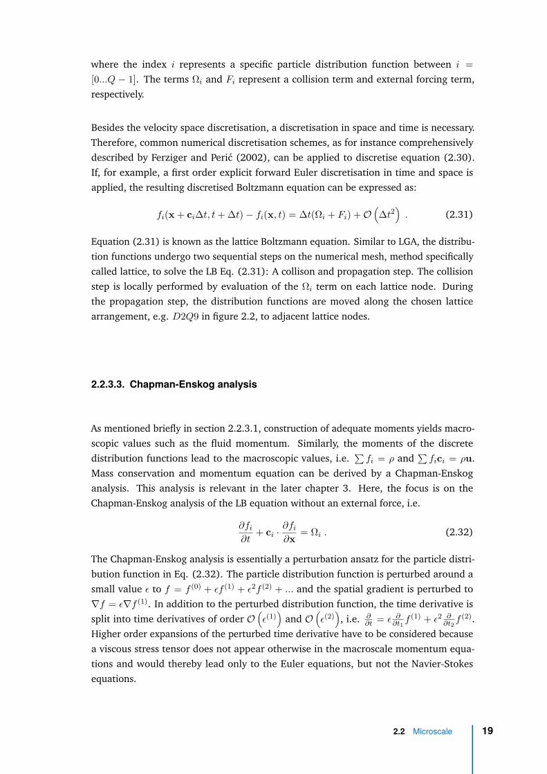
2.3 Sketch of bounce-back boundary condition . . . . . . . . . . . . . . . . . . . 21

2.4 Suspension system . . . . . . . . . . . . . . . . . . . . . . . . . . . . . . . . 41

3.1 Solid fraction computation for the partially saturated fluid-solid cell method 55

3.2 Setup of a single particle placed between two sheared walls to verify thestresslet computation . . . . . . . . . . . . . . . . . . . . . . . . . . . . . . 68

3.3 Single sphere stresslet Sxy and angular velocity errors Ωp over τ for a freelymoving particle and different lattice alignments NS and S. Piece-wise linearlines connecting the symbols are for visual guidance and not interpolationcurves. . . . . . . . . . . . . . . . . . . . . . . . . . . . . . . . . . . . . . . 70

3.4 LBM fluid velocity profiles of a free single particle in centre of shearedchannel. Simulation results are compared to the analytical solution. Insets:Fluid velocity profile for the same simulations shown from particle surfaceto channel wall where only every fourth lattice node is plotted . . . . . . . . 71

3.5 LBM hydrodynamic force profiles of a free single particle in centre of shearedchannel for a varing relaxation parameter. Insets: Shown is the solid fractionover the dimensionless channel height . . . . . . . . . . . . . . . . . . . . . 71

3.6 Stresslet error for varied lattice resolutions with a fixed subgrid resolutionand varied subgrid resolution for fixed lattice resolution . . . . . . . . . . 73

3.7 Single sphere stresslet and torque errors for varied τ for a fixed particle.Piece-wise linear lines connecting the symbols are for visual guidance andnot interpolation curves. . . . . . . . . . . . . . . . . . . . . . . . . . . . . 75

3.8 Hydrodynamic force profiles for a fixed particle in centre of a sheared channel 76

3.9 Simulation setup of two particles placed between two sheared walls to verifythe stresslet computation . . . . . . . . . . . . . . . . . . . . . . . . . . . . 78

3.10 Stresslet error of two freely rotating particles in shear flow for a variedrelaxation parameter . . . . . . . . . . . . . . . . . . . . . . . . . . . . . . 79

3.11 3D simulation setup of a sheared suspension illustrated on a slice throughthe domain . . . . . . . . . . . . . . . . . . . . . . . . . . . . . . . . . . . 80

xvii

3.12 Apparent viscosity for varied solid fractions of sheared frictionless mono-disperse suspensions. Piece-wise linear lines connecting the symbols are forvisual guidance and not interpolation curves. . . . . . . . . . . . . . . . . . 81

3.13 Dimensionless stress contributions for varying solid fractions for methodsBB and SP. . . . . . . . . . . . . . . . . . . . . . . . . . . . . . . . . . . . . 82

4.1 Simulation set-up to study normal lubrication forces between two particles 89

4.2 Dimensionless normal lubrication force and percent difference to the analyt-ical solution over the gap distance . . . . . . . . . . . . . . . . . . . . . . . 89

4.3 Normal lubrication force errors for particle motion aligned to lattice gridand diagonal to the lattice . . . . . . . . . . . . . . . . . . . . . . . . . . . 90

4.4 Particle location and the magnitude of the fluid velocity field for two particlesundergoing relative tangential motion . . . . . . . . . . . . . . . . . . . . . 91

4.5 Normal lubrication force for tangentially passing particles . . . . . . . . . 92

4.6 Tangential lubrication force for tangentially passing particles . . . . . . . . 92

4.7 Lubrication torque for tangentially passing particles . . . . . . . . . . . . . 93

4.8 Normal lubrication force for the case of rotating particles approaching eachother along the centre-to-centre line . . . . . . . . . . . . . . . . . . . . . 94

4.9 Lubrication force resulting from the particle rotation of rotating particlesapproaching each other along the centre-to-centre line . . . . . . . . . . . 94

4.10 Lubrication torque resulting from rotating particles approaching each otheralong the centre-to-centre line . . . . . . . . . . . . . . . . . . . . . . . . . 95

4.11 Normal lubrication force errors with corrections for different outer cut-offs 96

4.12 Normal lubrication force errors with cut-off corrections δcut = 0.75 fordifferent lattice resolutions . . . . . . . . . . . . . . . . . . . . . . . . . . . 96

4.13 Modified tangential lubrication force correction . . . . . . . . . . . . . . . 97

4.14 Modified torque due to sheared motion of particles . . . . . . . . . . . . . 98

4.15 Modified lubrication force correction for rotational interactions . . . . . . 98

4.16 Modified lubrication torque correction for rotational interactions . . . . . 99

5.1 Slice through a LBDEM simulation of a sheared suspension with Lees-Edwards boundary conditions showing particle distribution and fluid velocity109

5.2 Comparison of suspension viscosities for different solid fractions betweenGRM and simplified GRM models with different lubrication cutoff choicesfor low Reynolds number sheared dense suspensions . . . . . . . . . . . . 110

5.3 Stress contributions obtained from the GRM and simplified GRM modelsfrom corresponding simulations in Fig. 5.2 . . . . . . . . . . . . . . . . . . . 111

5.4 Frictionless suspension viscosity values for different solid fraction obtainedfrom low Reynolds number sheared LBDEM and DEM simulations . . . . . 113

5.5 Various stress contributions from the different frictionless LBDEM and DEMsimulations corresponding to Fig. 5.4 . . . . . . . . . . . . . . . . . . . . . 114

xviii

5.6 Frictional suspension viscosity values for different solid fraction obtainedfrom low Reynolds number sheared LBDEM and DEM simulations . . . . . 117

5.7 Various stress contributions from the different frictional LBDEM and DEMsimulations corresponding to Fig. 5.6 . . . . . . . . . . . . . . . . . . . . . 117

5.8 Contact and lubrication stress comparisons between LBDEM and DEM simu-lations for frictionless and frictional particle results . . . . . . . . . . . . . 119

5.9 Normal stress differences N1 and N2 from the corresponding LBDEM andDEM simulations in Fig. 5.6 . . . . . . . . . . . . . . . . . . . . . . . . . . 120

5.10 Different contributions to N1 and N2 normal stress differences obtainedfrom CLM-S and LBDEM where both include or exclude friction. . . . . . . 122

5.11 Fluid and particle velocity profiles of frictionless suspensions under simpleshear at a low Reynolds number Re = 0.1 and at a solid fraction φ = 0.3 . 125



6.1 (a): Dimensionless suspension viscosities obtained from frictionless sim-ulations employing a Hooke contact model at St = 0.1. Viscosity valuesare computed from the bulk stress. (b): Dimensionless viscosity values fordifferent St numbers from simulations with a Hooke contact model . . . . 133

6.2 (a)/(b): Dimensionless stress contributions at different solid fractions ob-tained from sheared simulations with a Hooke model and a Hertz model atSt = 0.1. (c): Dimensionless relationships between viscosity and solid frac-tion for the complete lubrication interaction model and a model consideringonly lubrication forces in normal collision direction . . . . . . . . . . . . . 134

6.3 (a): Dimensionless contact stress for varied St numbers obtained fromsimulations with a Hooke contact model. (b): Dimensionless contact stresscontributions for varied spring stiffnesses and changed contact models atSt = 0.1. (c): Parity plot of viscosities computed from bulk stress anddissipation for different contact models at St = 0.1 . . . . . . . . . . . . . 135

6.4 Probability density functions of dimensionless relative particle-particle ve-locities at different solid fractions obtained with a Hooke contact model atSt = 0.1 . . . . . . . . . . . . . . . . . . . . . . . . . . . . . . . . . . . . . 136

6.5 Probability density functions of dimensionless relative particle-particle ve-locities obtained from different contact modelling approaches at St = 0.1and solid fractions φ = 0.5 shown in (a) and φ = 0.62 presented in (b) . . 137

B.1 Illustration of the main coordinate system and geometrical relations tocompute lubricated interactions between particles . . . . . . . . . . . . . . 146

xix

List of Tables

2.1 Buckingham matrix for a suspension system . . . . . . . . . . . . . . . . . . 41

3.1 Moments of perturbed external forcing terms from two partially saturatedmethods . . . . . . . . . . . . . . . . . . . . . . . . . . . . . . . . . . . . . . 61

3.2 Integrated surface and volume stresslet parts over a freely moving sphere . 723.3 Integrated stresslet quadrants over a freely moving sphere . . . . . . . . . 723.4 Stresslet error for different domain sizes for the SP method . . . . . . . . . 733.5 Integrated stresslet parts over parts of a fixed sphere . . . . . . . . . . . . 77

xxi

Nomenclature

Abbreviations

BB method Non-equilibrium bounce-back method

BGK Bhatnagar-Gross-Krook model

CFD Computational fluid dynamics

DEM Discrete element method

DLM/FD Distributed Lagrangian Marker / Fictitious Domain

FDM Finite difference method

FVM Finite volume method

IBM Immersed boundary method

LB / LBM Lattice Boltzmann / Lattice Boltzmann method

LBDEM Coupled lattice Boltzmann discrete element method

LEbc Lees-Edwards boundary condition

MRT Multiple relaxation time model

PDF Partially saturated cell method

SBM Suspension balance model

SGR Subgrid resolution

SP method Superposition method

TRT Two relaxation time model

Calligraphic letters

M Mobility matrix

xxiii

R Grand resistance matrix

Greek letters

α Angular particle acceleration

βij Interphase momentum transfer coefficient

γ Particle size ratio

γn Damping coefficient for collision in normal direction

γt Damping coefficient for collision in tangential direction

γ Shear rate

δ Particle overlap

δc,i Inner cut-off for lubrication DEM model

δc,o Outer cut-off for lubrication DEM model

δcut LBDEM lubrication cut-off calibration parameter

εs Solid fraction on lattice node

ε Porosity in suspension system

εr Coefficient of restitution

εeff Effective coefficient of restitution

ηf Dynamic fluid viscosity

ηr Relative suspension viscosity

[η] Intrinsic viscosity

λ Mean free path

µr Coefficient of friction

µeff Effective friction coefficient

νf Kinematic fluid viscosity

ξ Velocity in (Boltzmann) velocity space

ρ Density in Boltzmann method

ρf Fluid density

ρp Particle density

xxiv

ρs Solid density

Σp Particle stress

σf Stress tensor of fluid phase

σs Stress tensor of solid phase

τ Relaxation time

φ Solid fraction in suspension system

ψ Independent variable

Ωfi Discrete lattice Boltzmann collision model for the fluid phase

Ωsi Discrete lattice Boltzmann collision model for the solid phase

ω∞ Fluid vorticity

ωi Lattice weighting function in lattice Boltzmann method

ω Angular velocity

Latin letters

B(x, τ) Weighting function for solid fraction on lattice node x

Bij Particle-specific friction coefficients

ci Velocity vector of discrete particle distribution function

cs Speed of sound in the lattice Boltzmann system

dp Particle diameter

deff Effective particle diameter

E Strain rate tensor

FB Force due to Brownian motion

FC Contact force

FH Hydrodynamic force

FL Lubrication force

Ffp,d Fluid-solid drag force

Ffp Fluid-solid interaction force

f(x, t) Particle distribution function

xxv

feq(x,u, t) Equilibrium particle distribution function

fi Discrete particle distribution function

feqi Discrete equilibrium particle distribution function

f−i Discrete particle distribution function in opposite direction of i

feq−i Discrete equilibrium particle distribution function in opposite directionof i

hgap Particle-particle gap distance

J Moment of inertia

k∗ Non-dimensionalised spring stiffness

kB Boltzmann constant

kn Spring stiffness in normal direction of collision

kt Spring stiffness in tangential direction of collision

Kn Knudsen number

m Mass

Ma Mach number

N Number of lattice cells over a particle diameter

p Pressure

pf Fluid pressure

ps Solid phase pressure

R Gas constant

rp Particle radius

reff Effective radius

Re Reynolds number

S Stresslet

St Stokes number

TC Contact torque

TH Hydrodynamic torque

xxvi

TL Lubrication torque

T Temperature

t Time

ub Boundary velocity

V Total volume of void spaces and solid body

Vp Particle volume

wi Discrete weighting function for the lattice Boltzmann directions

xl Lagrangian marker point

xp,c Particle centre of mass

xxvii

1Introduction

1.1 Motivation - suspensions in nature and industry

Suspensions, mixtures of a fluid and particles, behave very differently to Newtonianfluids such as water. The presence of particles suspended in a fluid, including Newtonianfluids, leads to many non-Newtonian characteristics of the overall suspension mixture.An example is an increased viscosity in comparison to a Newtonian fluid depending onthe solid fraction and even leading to a possibly jammed state when too many particlesare suspended. Other common characteristics are shear thinning, which means thatthe viscosity decreases for increasing shear rate, or shear thickening, which leads toan increasing viscosity with increasing shear rate. More effects and aforementionedsuspension behaviour have been subject in a plethora of research activities becausesuspensions are ubiquitous in nature and are a critical part in many important industrialapplications.

In nature, suspensions can be found in form of destructive mudslides or landslides andvolcanic flows. Prediction of mudslides and landslides could lead to precautions avoidingfatalities and infrastructural damages. Such infrastructural damages do not only lead tolocal socio-economic disruptions, but can have geographically widespread implicationsas exemplarily discussed by Winter et al. (2016) for landslide events in Scotland. Costscaused by mudslides and landslides accumulate to billion dollars as illustrated in figure1.1. Further losses, related to suspension flow in nature, are caused by sediment erosionin river beds and coastlines. For example, the European Commision (2009) reports thetremendous cost of 15.8 billion C in total expenses spent on coastal protections againstflooding and erosion over the period 1998-2015.

Apart from phenomena in nature, understanding of suspension flows is crucial in indus-trial applications. Endeavours to generate electricity from “green” sources, such as windpower or solar power, is undertaken by many governments to reduce the human carbonfootprint as agreed by a majority of nations in the global Paris climate agreement from2015. A major issue with “green” energy sources is the inherent unreliability and volatilityof power generation. However, a remedy could be efficient power storage by constructingeither pumped-storage plants or giant batteries. The latter solution could be realisedby fluid-solid Redox batteries which pump anode and cathode material, suspended asparticles in an electrolyte, through a membrane allowing only for electron exchange asdescribed by Duduta et al. (2011), Chalamala et al. (2014) and Hatzell et al. (2015).

1

Fig. 1.1.: Worldwide economic damage caused by mudslides according to and adopted fromCRED (n.d.).

An advantage of flow batteries is the possibility to scale the capable power storage bychanging correspondingly the tank sizes containing the cathode and anode materials.This is especially advantageous to common Lithium batteries when the required powerstorage capabilities are very large, cf. Chalamala et al. (2014).

Further knowledge about suspension flow behaviour is necessary in the productionprocess for Lithium battery packs which is described, for example, by Tagawa and Brodd(2009). During the Lithium battery production the electrode materials are mixed into afluid and the resulting slurry is coated onto a current collector sheet. The coated sheetsare subsequently exposed to a drying process to evaporate the fluid and thereby yieldingthe final electrode material which can be cut and compressed to battery cells. For efficientbatteries, knowledge about suspension handling is of high importance to achieve anoptimal coating surface.

The coating step in the battery production process is similar to an extrusion process.Extrusion processes are the most popular technique in additive manufacturing, commonlyknown as 3D-printing, according to Gibson et al. (2015). From the variety of additivemanufacturing techniques, extrusion processes squeeze either dry granular materials,molten materials, or suspensions through a nozzle to form layer by layer the requestedstructural shape.

2 Chapter 1 Introduction

1.2 Fluid-solid flow modelling approaches

Despite the enormous impact of suspension flows, or more generally expressed as fluid-solid or multiphase flows, a whole understanding is far from completeness. Althoughmuch research has been performed to gain a better insight into multiphase flow processes(cf. Hoef et al. (2008)), some knowledge gaps remain such as occurence of turbulence influid flows, let alone turbulence in multiphase flows. Besides experimental investigations,numerical methods are exceptionally useful and have become an exceedingly helpfultool due to a steady development of computational resources. However, fluid-solid floweffects are complex due to the vast range of length and time-scales involved. Therefore,numerical investigations of fluid-solid flows require a fine resolution of the differentlength and time scales (microscale) and result in a tremendous computational effortunless multiphase models are applied which allow for a coarser resolution of fluid-solidflow structures (meso- or macroscale). Yet, development of reliable multiphase flowmodels is hindered because of the very different scales. Construction of multiphasemodels has suffered under strict assumptions and thus complex processes have beeninadequately described (cf. Enwald et al. (1996), Hoef et al. (2008) and Hoef et al.(2006)).

Thus, various numerical approaches resolving different scales of fluid-solid flows existand can be classified into two basic groups: Eulerian and Lagrangian.

1.2.1 Fluid phase

According to Hoef et al. (2006), the choice of modelling approach in case of the fluidphase is determined by the Knudsen number

Kn = λ

L, (1.1)

where L is a characteristic length scale of the fluid flow and λ is the mean free path whichdescribes the average travelled distance of molecules between collisions. The mean freepath can be determined with the molecule density n (number of molecules per volume)and the scattering cross-section σSCS as λ = 1√

2nσSCSaccording to Gombosi (1994).

Very small Knudsen numbers Kn < 0.01 allow the application of continuum approaches,i.e. the application of the common mass/momentum/energy conservation equations influid mechanics. An increase of the free mean path of the molecules to 0.01 < Kn < 0.1leads to potential slip boundary conditions on the fluid-solid interface in contrast to theKn < 0.01 region where no-slip boundary conditions on the interface are fulfilled. Yet,the momentum conservation, i.e. the Navier-Stokes equations, are still valid. However,continuum assumptions are not legitimate for large Knudsen numbers Kn > 0.1 and

1.2 Fluid-solid flow modelling approaches 3

therefore the fluid is described by the fundamental Boltzmann equation, representingthe kinetic theory of molecular gases. Speaking in terms of Eulerian and Lagrangian,the Eulerian approach represents the continuum approach and the Lagrangian approachconfines molecular models.

1.2.2 Solid phase

In case of the solid phase, the Eulerian approach represents a continuum descriptionsimilar to the continuum approach for the fluid phase. E.g. Anderson and Jackson(1967) derived averaged continuum equations for the solid phase which are similar tothe commonly known mass conservation and Navier-Stokes equations. In the Lagrangianapproach however, the solid phase is described by discrete solid particles whose motionsare determined by Newton’s second law for motion.

1.2.3 Fluid-solid interaction modelling

Both the fluid phase and solid phase interact with each other and additionally solid-solidinteractions are common. The degree of necessary coupling in a model is describedby the solid volume fraction φ =

∑VpV which is the ratio of the total particle volume∑

Vp to the total volume V covered by particles and fluid (cf. Hoef et al. (2006)). Forφ < 10−6, only a so called one-way coupling is necessary, i.e. the solid volume fraction islow enough to consider only a fluid influence on the particles and to neglect a reciprocalparticle influence as well as particle-particle interactions. Higher solid volume fractions10−6 < φ < 10−3 require consideration of the particle influence on the fluid flow inaddition to the impact of fluid flow on the particle motion. However, the particle-particlecollisions are still neglected in this two-way coupling approach. In four-way coupledsystems, which are highly relevant for industrial processes, particle-particle interactionsare, besides a mutual fluid-particle coupling, significant in systems of φ > 10−3.

1.3 Multiscale models

In the previous section, the two different general modelling approaches, Eulerian andLagrangian, for solid and fluid phase are elucidated. In fluid-solid flows, the approachesfor the phases do not have to be the same and can be chosen in different combinations.However, phases interact with each other and formulation of the interactions dependsstrongly of the chosen combination of modelling approaches.

The most fundamental modelling approach is a combination of Lagrangian-Lagrangianmodels (cf. Hoef et al. (2008)), i.e. suspended solid phase and fluid phase are representedby particles. This leads to a molecular description of the fluid flow. The flow of both


phases is determined by solution of Newton’s second law for motion for each particle andthe interaction between both phases is a result of the particle collisions. An extremelyfine resolution of the multiphase flow processes is obtained by the Lagrangian-Lagrangianapproach. In fact, according to Hoef et al. (2008), the resolved scales are so fine in theLagrangian-Lagrangian approach that it is only relevant in cases of a strong influence ofthermal fluctuations of the fluid phase on the motion of the solid particles.

Description of fluid-solid flows on a slightly larger scale leads to the so called resolvedEulerian-Lagrangian approach (cf. Hoef et al. (2008)). In this kind of direct numericalsimulation, the fluid flow is determined on a numerical mesh (Eulerian viewpoint) withcell sizes smaller than the actual solid particle sizes, whereas the solid particles aretracked by the Lagrangian approach. The interaction between the phases is achieved bya no-slip boundary condition of the fluid on the particle surfaces.

Direct numerical simulations (DNS), which resolve all fluid structures, allow for validationand development of multiphase models, e.g. Derksen and Sundaresan (2007) used thistechnique to evaluate two-fluid model closures. Furthermore, DNSs are helpful forinvestigations of physical phenomena or processes on microscale, e.g. sediment erosion(cf. Kidanemariam and Uhlmann (2014)) or heat transfer in fluid-particle flows (cf.Deen et al. (2012), Deen and Kuipers (2014)). However, DNSs require tremendouscomputational efforts and are thus not feasible for engineering applications. Yet, DNSsare an invaluable technique to construct models on a larger scale (cf. Deen and Kuipers(2014)).

Models on a larger scale include unresolved Eulerian-Lagrangian approaches and Eulerian-Eulerian approaches (cf. Hoef et al. (2008)). The former approach is similar to theresolved Eulerian-Lagrangian approach, but differs in that the mesh cell size of theEulerian grid is larger than the particle sizes and therefore confines several particlesin one cell. This leads to an averaged fluid flow field. The particles are describedby a Lagrangian approach. On this basis, the coupling between fluid and particles isperformed by closure terms (e.g. drag closure). These unresolved Eulerian-Lagrangianapproaches are computational less costly than direct numerical simulations, but are stillrather applied to laboratory scale experiments than full-scale engineering tasks (cf. Hoefet al. (2008)).

Eulerian-Eulerian approaches known as two-fluid models are useful to simulate engi-neering fluid-solid flow problems. In a fluid-particle flow, both phases are modelledas separate continua whose interactions have to be considered not only in a fluid-solidclosure, but also in a solid-solid closure. The advantage of such an approach is therequirement of much less computational power than more detailed approaches. However,one drawbacks is the necessity of an adequately developed and calibrated model for the

1.3 Multiscale models 5

investigating problem. Moreover, only a narrow range of physical parameters and effectscan be considered due to limited closure modelling capabilities.

1.4 Aim & structure of thesis

The aim of this thesis is on one hand to study and develop the capabilities of the discreteelement method and partially saturated lattice Boltzmann method couplings to simulatedense suspensions. On the other hand, this thesis aims to show how aforementionedmethodologies can be be used to investigate physical microscale processes affecting thebulk behaviour of dense suspensions. Therefore, the following chapter 2 discusses thenecessary fundamentals - micro-macro-scale transition, simulation methods on microscale,and modelling approaches on macroscale. The subsequent result chapters 3-6 of thisthesis are written in article form for publication reasons in journals. Hence, the chapterscontain separate introduction, methodology, and conclusion sections. In chapter 3, twopartially saturated lattice Boltzmann methods to simulate suspensions are theoreticallyand numerically evaluated with regard to the stresslet computation and its effect onthe bulk viscosity of suspensions. In chapter 4, the partially saturated lattice Boltzmannmethod is evaluated and calibrated in terms of simulation capabilities of lubricationforces between two particles. Thereafter, sheared simulations of dense suspensions areconducted with a discrete element method, employing a lubrication force model, and theprevious evaluated coupled lattice Boltzmann discrete element method. A comparisonbetween both simulation approaches is performed showing that dense suspensions can bealso simulated by a discrete element method with additional lubrication force modelling.In the last results chapter, the DEM with lubrication force modelling is employed to studyand explain the viscosity divergence for increasing solid fraction in dense suspensionsand thereby also demonstrating its usefulness to simulate dense suspensions. The thesisfinishes with a summary and conclusion chapter which is followed by recommendationsfor possible future work.


2Fundamentals & literature review

2.1 Coarse graining

In general, reducing the degrees of freedom of a system is described as coarse graining. Influid-solid flows, the various Lagrangian and Eulerian methods, described in the previoussections, resolve the fluid and solid phases on different length scales. Bridging thedifferent scales for modelling purposes or combining different methods to hybrid methodscan be achieved by coarse-graining of flow parameters, i.e. transferring properties froma fine resolved scale (microscale) to a coarse resolved scale (meso- or macroscale).

2.1.1 Averaging techniques

Coarse-graining requires the averaging of variables. An overview of averaging techniquesis provided by, for instance, Drew (1983), Enwald et al. (1996) and Pope (2000), and arecap is given here.

A volume average of a variable f(x, t) at location x and time t is defined as:

〈f〉V (x, t) = 1V

∫Vf(x, t) dV , (2.1)

where the averaging process takes place at a time t around the location x in the volumeV . The dimensions of averaging volume V should be between the characteristic lengthscales of the phases and the length scales of the system.

Similar, a time average at a location x over a time interval ∆t reads

〈f〉t(x, t) = 1∆t

∫ t+∆t/2

t−∆t/2f(x, t) dt . (2.2)

Additionally, there is the possibility to apply an ensemble average:

〈f〉E(x, t) = limN→∞

1N

N∑n=1

f (n)(x, t) , (2.3)

which yields the average of N conducted experiments with regard to the variable f(x, t)at location x and time t.

7

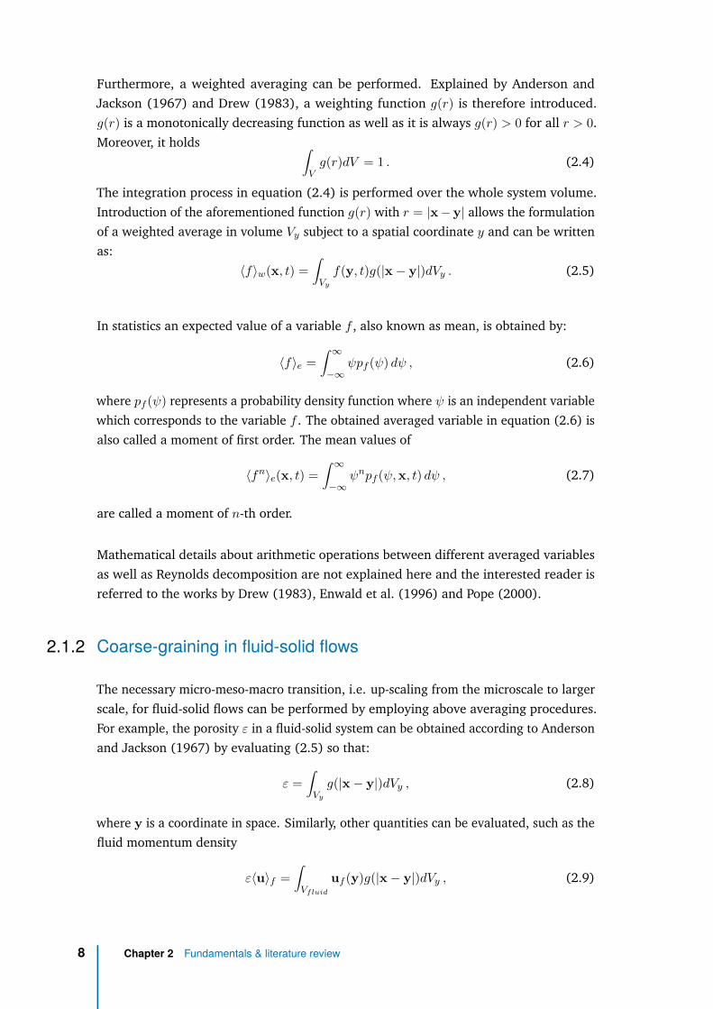
Furthermore, a weighted averaging can be performed. Explained by Anderson andJackson (1967) and Drew (1983), a weighting function g(r) is therefore introduced.g(r) is a monotonically decreasing function as well as it is always g(r) > 0 for all r > 0.Moreover, it holds ∫

Vg(r)dV = 1 . (2.4)

The integration process in equation (2.4) is performed over the whole system volume.Introduction of the aforementioned function g(r) with r = |x−y| allows the formulationof a weighted average in volume Vy subject to a spatial coordinate y and can be writtenas:

〈f〉w(x, t) =∫Vyf(y, t)g(|x− y|)dVy . (2.5)

In statistics an expected value of a variable f , also known as mean, is obtained by:

〈f〉e =∫ ∞−∞

ψpf (ψ) dψ , (2.6)

where pf (ψ) represents a probability density function where ψ is an independent variablewhich corresponds to the variable f . The obtained averaged variable in equation (2.6) isalso called a moment of first order. The mean values of

〈fn〉e(x, t) =∫ ∞−∞

ψnpf (ψ,x, t) dψ , (2.7)

are called a moment of n-th order.

Mathematical details about arithmetic operations between different averaged variablesas well as Reynolds decomposition are not explained here and the interested reader isreferred to the works by Drew (1983), Enwald et al. (1996) and Pope (2000).

2.1.2 Coarse-graining in fluid-solid flows

The necessary micro-meso-macro transition, i.e. up-scaling from the microscale to largerscale, for fluid-solid flows can be performed by employing above averaging procedures.For example, the porosity ε in a fluid-solid system can be obtained according to Andersonand Jackson (1967) by evaluating (2.5) so that:

ε =∫Vyg(|x− y|)dVy , (2.8)

where y is a coordinate in space. Similarly, other quantities can be evaluated, such as thefluid momentum density

ε〈u〉f =∫Vfluid

uf (y)g(|x− y|)dVy , (2.9)

8 Chapter 2 Fundamentals & literature review

where uf is the fluid velocity at position y, or solid fluid momentum density

ε〈u〉s =∫Vparticles

us(y)g(|x− y|)dVy , (2.10)

Hitherto, the discussion about coarse-graining has included the whole simulation domain.However, in some cases it is required to average only over specific volume elements,e.g. separate volumes close to walls to filter out wall effects or for coupled Eulerian-Lagrangian methods for which the numerical mesh might define fluid volume elements.Therefore, different coarse-graining methods for fluid-solid flows have been developed.E.g. Sun and Xiao (2015) discuss, mostly for unresolved Eulerian-Lagrange simulations,popular coarse-graining methods for the particle phase, such as the particle centroidmethod, the divided particle volume method, the two-grid formulation, the statisticalkernel method, and the diffusion-based coarse graining method. All methods should fulfilto some extent the following criteria: Conserve physical quantities such as particle massor particle momenta, flawless coarse graining near boundaries, mesh-independent results,simple implementation into numerical solvers, and achieve smooth coarse grained fields.The first two criteria are of highest importance in order to reproduce correctly all physicalproperties. The remaining criteria are preferably also fulfilled to achieve an overallexcellent coarse-graining method, albeit achievement is not a strict necessity to obtain aphysical correct method.

2.2 Microscale

2.2.1 Particle dynamics

Popular methods to investigate the solid phase characteristics on microscale are inelastichard-sphere models, also referred to as event-driven method, and soft-sphere modelsaccording to Herrmann and Luding (1998), Luding (2004), Pöschel and Schwager (2005)and Andreotti et al. (2013). The former method is based on instantaneous collisionsbetween rigid particles. The particle momentum exchange occurs for only two particlesin contact and hence the hard-sphere model is used for dilute particle systems. In soft-sphere models, contact forces between spheres are determined from the particle-particleoverlap. A soft-sphere model requires therefore a fine time-step resolution leading toextensive computational overhead. Although not recommendable to simulate diluteparticle systems, the soft-sphere model is widely used to simulate multi-particle contactsas they are found in for example dense suspensions. Hence, the hard-sphere model isdescribed only very briefly in contrast to the soft-sphere model in the remainder of thissection.

2.2 Microscale 9

2.2.1.1. Hard-sphere method

As above mentioned, collisions with the event-driven method occur instantly and themomentum between particles is exchanged instantly at contact. For a particle-wallcollision in direction of the wall normal vector, a coefficient of restitution εr can bedefined which describes the rebound of the particle from the wall by setting the normalpost-collision velocity of a particle u′

p,n in relation to the normal pre-collision velocityup,n:

εr =u′p,n

up,n. (2.11)

Similarly, the post-velocities of particles with same diameter and mass for collisions alongthe particle centre-to-centre line can be determined:

u′

p,1/2,n = up,1/2,n ∓1 + εr

2 (up,1,n − up,2,n) . (2.12)

Differences in physical and geometrical properties of the particles, rotation, and obliquecollisions, which require also modelling of tangential forces, can be considered in hard-sphere models and the interested reader is referred to the works of Herrmann and Luding(1998) and Pöschel and Schwager (2005) for more details.

2.2.1.2. Soft-sphere method

Soft-sphere modelling was introduced by Cundall and Strack (1979) and is widely knownas discrete element method (DEM). The theory is based on Newton’s equations for motionin translational,

mi∂x2

i

∂2t= Fi =

∑i

FCi +

∑i

FLi , (2.13)

and rotational motion,

Ji∂ωi∂t

= Ti =∑i

TCi +

∑i

TLi , (2.14)

where mass, position, moment of inertia and angular velocity of particle i are describedby mi, xi, Ji and ωi, respectively. Both equations are applicable to particles of any shape.The total force and torque is a superposition between various contributions, such asparticle-particle contacts

∑i FC

i /∑i TC

i or lubrication interactions between particles∑i FL

i /∑i TL

i . Lubrication theory is succinctly described in the next section 2.2.2 andlubrication modelling in DEM is discussed in chapter 5.

Contact modelling for overlapping particles is an essential part in DEM simulations anddifferent models have been proposed. The most widely used models are a Hooke andHertz model as described by Luding (1998) and Herrmann and Luding (1998). In normal


direction of the collision, which is along the particle centre-to-centre line, the Hookemodel relates the particle overlap δ to a linear spring force with the spring stiffness knand relates the relative collision velocity to a dashpot model with the damping coefficientγn. In tangential direction, forces are analogously with a spring kt and dashpot γt modelconstructed leading to the final expression:

FCHooke = (knδn + γnup,rel,n)− (ktδt + γtup,rel,t) . (2.15)

The Hertz model modifies the Hooke model to a non-linear model by multiplication of√δnreff , i.e.

FCHertz =

√δnreff

FC,Hooke , (2.16)

where the effective particle radius is reff = rirjri+rj . Schäfer et al. (1996) investigated

the spring stiffnesses choice on the collision dynamics and by analysis of the oscillationperiods showed that the tangential stiffness is ideally chosen as a function of the normalspring stiffness according to an optimal relation kt = 2

7kn which leads to similar oscilla-tions in normal and tangential direction. The relation kt = 2

7kn might not be the idealchoice as recently shown by Thornton et al. (2011), but is commonly used in the DEMliterature.

A key component to simulate realistic behaviour of granular materials is consideration ofstatic friction between particles by an additional Coulomb friction criterion:

|FCt | ≤ |µrFC

n | . (2.17)

The tangential contact force FCt is thereby limited by the product of coefficient of

friction µr and absolute contact normal force. However, the literature differs in whichforce contributions are considered for the normal and tangential forces in the Coulombcriterion. Cundall and Strack (1979) evaluate the normal force in the Coulomb criterion(2.17) as the normal spring force FC

n = knδn and make similarly use of the tangentialspring force for the tangential force FC

t = min(ktδt, µrFCn ). Slightly different, Herrmann

and Luding (1998) suggest to evaluate the Coulomb criteria based on the normal forcecomprising spring and dashpot force, i.e. FC

n = knδn + γnup,rel,n, but consider onlythe tangential spring force, i.e. Fk,t = ktδt. Although the aforementioned differentCoulomb criterion proposals are exemplarily discussed for the Hooke model, the verysame separation of spring and dashpot force contributions for the normal and tangentialforces applies for the Hertz model.

Besides the above described contact models, many additional force models to includedifferent physical effects have been proposed. In this work, the particle interactions arelimited to mechanical contact and lubrication forces. Hence, a detailed discussion is notcarried out here and only the major models are mentioned here for reference purposes. In

2.2 Microscale 11

simulations carried out in this work, particles are of spherical shape. However, in realityparticles are found to have all kind of complex forms. In DEM, non-sphericity of particlescan be either modelled by introduction of rolling friction models while using sphericalparticles as discussed by Ai et al. (2011) or by modelling the complex non-sphericalshape. Therefore, non-spherical particle shape can be modelled by polygons according toCundall (1988) or superquadrics according to Williams and Pentland (1992), or the non-spherical particles are constructed from multiple spherical particles as suggested by Favieret al. (1999) and Jensen et al. (1999). Further modelling approaches for non-sphericalparticles are possible and discussed in a review by Lu et al. (2015). Apart from particleshape effects in granular flows, the contact between particles can be more complexthan previously described. Particles can undergo adhesive, elastic-plastic collisions andcontact models capturing such behaviour have been proposed, e.g. by Luding (2005)and Thakur et al. (2014). Furthermore, other non-contact interaction forces relevantfor cohesion, e.g. van-der-Walls forces, electrostatic forces, liquid bridge forces, canbe considered in simulations and are discussed by Zhu et al. (2007). Although manydifferent geometrical and physical properties can be considered between particles, thecaveat of DEM simulations is careful calibration of the various model parameters toobtain correct bulk scale quantities as discussed in a calibration review for DEM byCoetzee (2017).

2.2.2 Lubricated particle interactions & Stokesian Dynamics

Two surfaces separated by a fluid, for example in lubricated bearings, experience amotion resisting force when squeezed together due to an increased pressure build up inthe fluid. Similarly, particles in close contact affect each others’ kinematics due to indirectinteractions through an interstitial fluid. Lubrication interactions are a fundamental partof suspension flows and hence, have been research subject for decades.

Theoretical analysis to derive expressions for lubrication interactions have been under-taken for smooth, rigid, spherical particles in low Reynolds number flows so that theNavier-Stokes equations could be considerable simplified. Solutions for the Stokes equa-tions / creeping flow equations can be determined by series expansion techniques, suchas asymptotic expansion or multipole expansion. Brenner (1961) deduced thereby thehydrodynamic interaction force on a sphere while steadily moving aforementioned spheretowards or from a wall or free surface. Solutions for parallel motion of a sphere alonga planar wall with regard to translational and rotational motion as well as expressionsfor hydrodynamic force and torque were found by O‘Neill and Stewartson (1967) andGoldman et al. (1967a). The theory derived by Goldman et al. (1967a) also shows thatwith the above assumptions the moving sphere cannot touch the wall. Furthermore,Goldman et al. (1967b) extended the solutions for a wall undergoing shearing motion.Cox and Brenner (1967) determined more accurate solutions for the hydrodynamic force


on a sphere approaching a wall for very small gap distances by dividing the expansioncalculations into an “inner” and “outer” region, depending on the wall-particle distance.Hydrodynamic forces on two particles, of which one is fixed, were analysed by Cooleyand O’Neill (1969). Hansford (1970) studied the hydrodynamic forces for two equallysized spheres approaching each other with the same velocities along the centre-to-centreparticle line by dividing expansion techniques into an inner and outer regime as intro-duced by Cox and Brenner (1967). Jeffrey (1982) determined accurately higher ordersolutions for the hydrodynamic forces on two bi-disperse sized spheres which approacheach other with equal velocities. Moreover, Jeffrey (1982) compared derived expressionsto previous numerical calculations for different particle size ratios to find numericalvalues for constant terms in the expanded solutions.

Brenner and O‘Neill (1972) introduced a general formulation to determine hydrodynamicforces and particle velocities for multi-particle systems. Therefore, a grand resistancematrix R for determination of hydrodynamic forces in dependency of the particlevelocities and fluid background shear velocity were developed. Furthermore, a shearresistance matrix, or also so called mobility matrix, which is the inverse of the grandresistance matrix, M = R−1 to determine particle velocities in dependency of thehydrodynamic forces was introduced. The hydrodynamic forces can be in the simplestform expressed as:

F = R ·U , (2.18)

where the force matrix on the left-hand side and the velocity matrix on the right-handside have N force and velocity vectors for N particles. The grand resistance matrix hasthus N ×N elements. The torque is analogously determined.

Further work with regard to the resistance matrix formulation and calculation of matrixelements was conducted by Majumdar and O‘Neill (1972),Cox (1974), and Batchelor(1976) who tried to merge previous literature in terms of the grand resistance matrixformulation. Jeffrey and Onishi (1984) provide an overview of the grand resistancematrix formulation for hydrodynamic forces and torques as well as for the mobilitymatrix for translational and angular particle velocities with detailed calculations of thematrix elements for bi-disperse two particle pair interactions. Jeffrey (1992) extended theprevious work on the resistance and mobility matrix formulation to incorporate strain rateeffects and expressions for the stresslet values in a two particle system. For the interestedreader the very detailed and comprehensive overview of lubrication interactions, theirderivations and general formulation in grand resistance matrix formulation by Kim andKarrila (2005) is strongly recommended. In chapter 5, the idea and details of the grand-resistance matrix formulation are revisited to simulate dense suspensions through themeans of a DEM.

In Stokesian dynamics, developed by Bossis and Brady (1984) and Brady and Bossis(1988), the grand-resistance matrix for pairwise particle-particle interactions is used to

2.2 Microscale 13

determine the motion of inertialess particles. The particle motion can be described byNewton’s second law, i.e.

m∂x2

∂2t= FH + FC + FB . (2.19)

Besides hydrodynamic forces FH , contact forces FC for colliding particles and forcesfrom Brownian motion FB can be considered. For inertialess particles, valid for lowReynolds number flows, the left-hand side vanishes and Eq. (2.19) can be re-written bysubstitution of Eq. (2.18) to:

0 = R ·U + FC + FB , (2.20)

which leads to the following expression for the particle velocities:

U = −R−1 ·(FC + FB

). (2.21)

The particle positions are updated for every timestep from Eq. (2.21). However, theStokesian dynamics method requires computation of the inverse grand resistance matrixat every single timestep due to its dependency of the geometrical relations, distance andsize ratio, between particles.

The above discussion about lubrication forces is based on the assumption of smooth par-ticles. In reality however, particles exhibit a surface roughness and the surface asperitiesare commonly of the size 10−2 to 10−3 of a particle radii according to measurements ofSmart and Leighton Jr. (1989). Such particle asperities can lead to changed interactionsbetween particles and thereby to changed particle trajectories as shown by Da Cunhaand Hinch (1996). Thus, changed particle interactions due to surface roughness lead toa change in suspension rheology with normal stress differences not found for smoothparticles and reduced suspension viscosities for increased surface roughness accordingto Davis et al. (2003). However, Tanner and Dai (2016) reported in contrast to Daviset al. (2003) increased suspension viscosities for rough particles. The opposing resultscould be possibly explained by different friction conditions. The friction is unchangedfor changed asperity sizes in the analysis conducted by Davis et al. (2003) whereas thefriction coefficients of the particles used in the experiments by Tanner and Dai (2016)are not measured and hence not stated. However, Tanner and Dai (2016) mention in theintroduction that an increased roughness could be related to increased friction whichcould explain the different findings to Davis et al. (2003).

Besides surface roughness, particle inertia affects particle-particle collisions within a fluid.Previous work on particles colliding with a wall immersed in a fluid, e.g. numerical workby Davis et al. (1986) and experiments conducted by Joseph et al. (2001) and Gondretet al. (2002), shows that the collision and particle rebounce depend only to some weakextent on the particle material and that it can be classified according to a Stokes numberSt = mpU0

6πµf r2p

where mp is the particle mass, U0 is the approaching velocity, µf the fluid


viscosity, and rp is the particle radius. For Stokes numbers below a value of aroundten, the rebound of a sphere is strongly affected by the fluid leading to no observablerebound. For Stokes numbers larger than ten, the fluid influence on the rebound startsto decrease. An effective coefficient of restitution εeff = εwet

εdrycan be defined where the

coefficient of restitution is defined as the ratio of impact velocity Uimpact and reboundvelocity Urebound, i.e. ε = Urebound

Uimpact. For increasing Stokes numbers the effective coefficient

of restitution increases and asymptotically converges towards εeff = 1 for very largeStokes number St > O(1000), i.e. the fluid influence is irrelevant as the rebounce cannotbe differentiated to dry collisions. The altered collision behaviour and the influenceof particle surface roughness on the collision is attempted to be described in changedcollision models obeying elastohydrodynamic lubrication theory, e.g. Yang (2006) andreferences therein.

2.2.3 Lattice-Boltzmann Method (LBM)

2.2.3.1. Basic theory

A fundamental approach to describe fluids are lattice-gas models / lattice-gas automaton(LGA). In LGAs the fluid molecules are represented by fictitious molecules, called discreteBoolean elements, with discrete locations and velocities. The single Boolean elementsare placed on nodes of a lattice (cf. figure 2.1). As described by Frisch et al. (1986),the LGA procedure consists of two repeating steps: Propagation and collision. In thepropagation step the discrete elements are moved along the node connections into thedirection of their velocity vectors. In the following collision step, the collisions betweendiscrete elements, which are located on the same node, are computed. The number ofdiscrete elements and the corresponding momentum are conserved during the collisionprocesses.

Simulations with LGA are very detailed and applying LGA on larger scales is not viable.However, instead of using discrete Boolean elements, the discrete Boolean elements canbe statistically summarised in particle distribution functions, as elucidated by McNamaraand Zanetti (1988). Therefore, the molecules of the fluid are ensemble averaged, andthe evolution of the particle distribution function in space and time can be described bythe Boltzmann equation:

∂f

∂t+ ξ · ∂f

∂x + Fm· ∂f∂ξ

=(∂f

∂t

)coll

. (2.22)

This fundamental gas-kinetic transport equation was derived by Boltzmann (1872) wherethe left-hand side represents the substantial derivative of the particle distribution functionf and a collision term is found on the right-hand side.

2.2 Microscale 15

Fig. 2.1.: Lattice for a lattice-gas automata. Elements with a single arrow represent the actualtime step, whereas elements with a double arrow are the following timestep. Adoptedfrom Frisch et al. (1986).

The particle distribution function f(x, ξ, t) in the Boltzmann equation provides infor-mation about the mass of molecules with velocity ξ at location x at time t, i.e. thedistribution function has in a three-dimensional physical space and three-dimensionalvelocity space the units [f ] = mass

length3×(length/time)3 = mass×time3

length6 . This means that anintegration over the whole physical space x and velocity space ξ yields the mass m ofmolecules in the system:

m =∫ξ

∫xf(ξ,x, t) dx dξ . (2.23)

As one is usually more interested in quantities on the macroscale than on the microscale,equation (2.23) can be generalised by taking moments of the particle distribution functionaccording to equation (2.7). Thereby, the macroscopic density

ρ(x, t) =∫ξ0f(x, ξ, t)dξ (2.24)

or the macroscopic momentum

ρ(x, t)u(x, t) =∫ξ1f(x, ξ, t)dξ (2.25)

can be evaluated.

In LGA the collisions occur between single molecules, whereas in the Boltzmann equation,the collision process between molecules results in a change of the particle distributionfunction f(x, c, t). A change in the distribution function due to collision is expressedin the collision term on the right-hand side of the Boltzmann equation and has to bemodelled. The approach to model the collision term suggested by Boltzmann (1872)is based on the collision between two elastic particles which are uncorrelated beforecollision. The derivation can be either found in Boltzmann (1872) or Lieberman and


Lichtenberg (2005) and the final collision integral can be written according to Liebermanand Lichtenberg (2005) as:(

∂f

∂t

)coll

=∫d3v2

∫ 2π

0dφ1

∫ π

0(f ′

1f′2 − f1f2)|v1 − v2|Isinθ1dθ1 (2.26)

where the particles have the relative velocity |v1 − v2| and the particle distributionfunction of the colliding particles after the collision is given by f

′1 and f

′2 and before the

collision by f1 and f2. However, evaluation of the collision integral (2.26) is difficultand simpler collision term models have been suggested. Different collision terms arediscussed in the later subsection 2.2.3.6, but for the sake of elucidating the Chapman-Enskog expansion in section 2.2.3.3, a common simplified expression for the collision termis introduced here. The widely known Bhatnagar-Gross-Krook (BGK) model proposed byBhatnagar et al. (1954) which reads:(

∂f

∂t

)coll

= feq − fτ(v) , (2.27)

where the particle distribution function f is relaxed towards a local equilibrium feq overa collision relaxation time τ . The equilibrium function feq can be determined by thesolution of the Boltzmann equation in the special case of thermodynamic equilibriumand has for mono-atomic collisions a Maxwell distribution:

feq(x, |v|, t) = ρ

( 12πRT

)3/2e−|v|

2/(2RT ) , (2.28)

where R and T are the gas constant and the temperature, respectively.

2.2.3.2. Discretised Boltzmann equation

The Boltzmann equation in continuous form, i.e. Eq. (2.22), is difficult to evaluatebecause the particle distribution function spans over seven dimensions. However, itis simpler to solve the equation numerically and therefore, discretisation in velocityspace, physical space, and time are required. The procedure to discretise the Boltzmannequation has been extensively elucidated in the literature, e.g. Wolf-Gladrow (2000),Succi (2001) and Krüger et al. (2017), and instead of reiterating all the details, only thekey points are provided here. The discretisation of the velocity space follows basicallythe following points:

1. Non-dimensionialise the Boltzmann equation (2.22)

2. An equilibrium function can be determined from the Boltzmann equation for anequilibrated system, resulting in a Maxwell distribution

2.2 Microscale 17

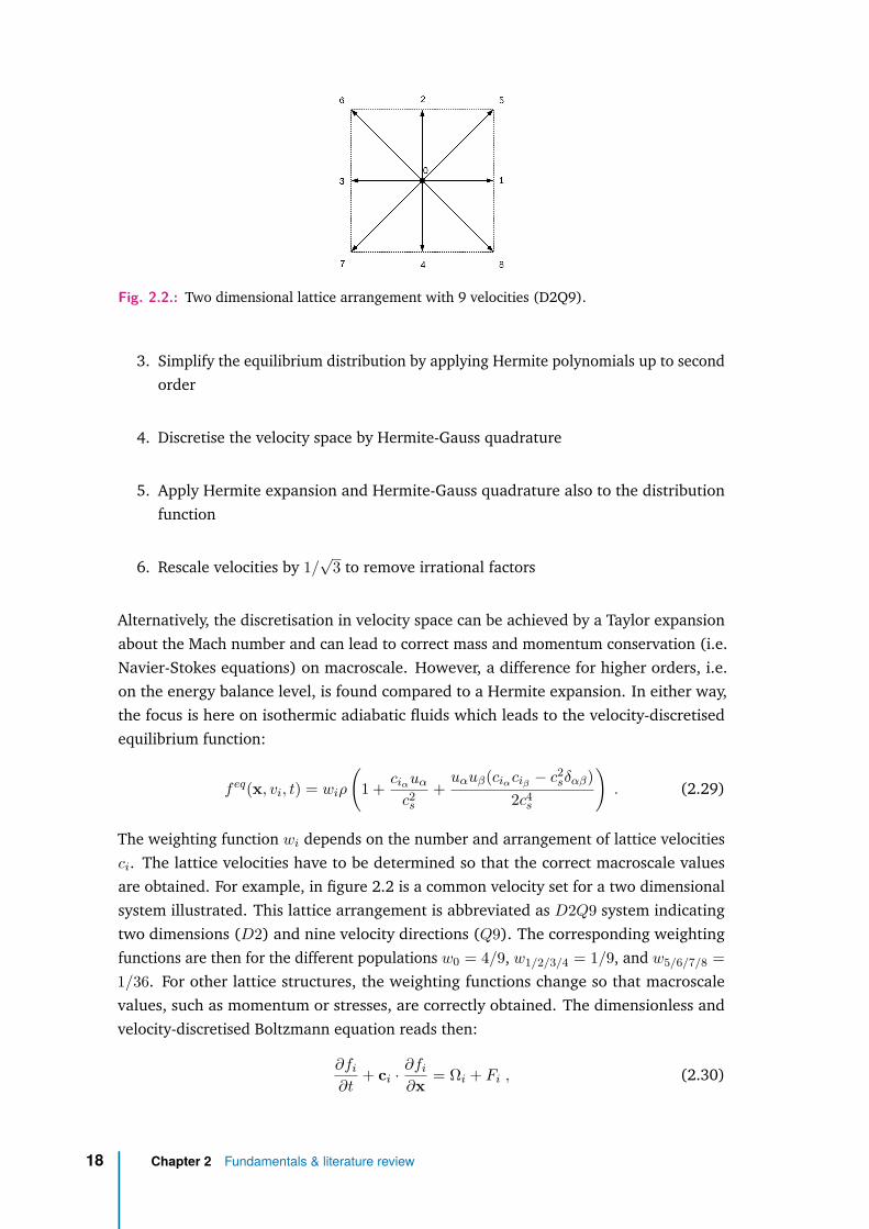
Fig. 2.2.: Two dimensional lattice arrangement with 9 velocities (D2Q9).

3. Simplify the equilibrium distribution by applying Hermite polynomials up to secondorder

4. Discretise the velocity space by Hermite-Gauss quadrature

5. Apply Hermite expansion and Hermite-Gauss quadrature also to the distributionfunction

6. Rescale velocities by 1/√

3 to remove irrational factors

Alternatively, the discretisation in velocity space can be achieved by a Taylor expansionabout the Mach number and can lead to correct mass and momentum conservation (i.e.Navier-Stokes equations) on macroscale. However, a difference for higher orders, i.e.on the energy balance level, is found compared to a Hermite expansion. In either way,the focus is here on isothermic adiabatic fluids which leads to the velocity-discretisedequilibrium function:

feq(x, vi, t) = wiρ

(1 + ciαuα

c2s

+uαuβ(ciαciβ − c2

sδαβ)2c4s

). (2.29)

The weighting function wi depends on the number and arrangement of lattice velocitiesci. The lattice velocities have to be determined so that the correct macroscale valuesare obtained. For example, in figure 2.2 is a common velocity set for a two dimensionalsystem illustrated. This lattice arrangement is abbreviated as D2Q9 system indicatingtwo dimensions (D2) and nine velocity directions (Q9). The corresponding weightingfunctions are then for the different populations w0 = 4/9, w1/2/3/4 = 1/9, and w5/6/7/8 =1/36. For other lattice structures, the weighting functions change so that macroscalevalues, such as momentum or stresses, are correctly obtained. The dimensionless andvelocity-discretised Boltzmann equation reads then:

∂fi∂t

+ ci ·∂fi∂x = Ωi + Fi , (2.30)


where the index i represents a specific particle distribution function between i =[0...Q − 1]. The terms Ωi and Fi represent a collision term and external forcing term,respectively.

Besides the velocity space discretisation, a discretisation in space and time is necessary.Therefore, common numerical discretisation schemes, as for instance comprehensivelydescribed by Ferziger and Peric (2002), can be applied to discretise equation (2.30).If, for example, a first order explicit forward Euler discretisation in time and space isapplied, the resulting discretised Boltzmann equation can be expressed as:

fi(x + ci∆t, t+ ∆t)− fi(x, t) = ∆t(Ωi + Fi) +O(∆t2

). (2.31)

Equation (2.31) is known as the lattice Boltzmann equation. Similar to LGA, the distribu-tion functions undergo two sequential steps on the numerical mesh, method specificallycalled lattice, to solve the LB Eq. (2.31): A collison and propagation step. The collisionstep is locally performed by evaluation of the Ωi term on each lattice node. Duringthe propagation step, the distribution functions are moved along the chosen latticearrangement, e.g. D2Q9 in figure 2.2, to adjacent lattice nodes.

2.2.3.3. Chapman-Enskog analysis

As mentioned briefly in section 2.2.3.1, construction of adequate moments yields macro-scopic values such as the fluid momentum. Similarly, the moments of the discretedistribution functions lead to the macroscopic values, i.e.

∑fi = ρ and

∑fici = ρu.

Mass conservation and momentum equation can be derived by a Chapman-Enskoganalysis. This analysis is relevant in the later chapter 3. Here, the focus is on theChapman-Enskog analysis of the LB equation without an external force, i.e.

∂fi∂t

+ ci ·∂fi∂x = Ωi . (2.32)

The Chapman-Enskog analysis is essentially a perturbation ansatz for the particle distri-bution function in Eq. (2.32). The particle distribution function is perturbed around asmall value ε to f = f (0) + εf (1) + ε2f (2) + ... and the spatial gradient is perturbed to∇f = ε∇f (1). In addition to the perturbed distribution function, the time derivative issplit into time derivatives of order O

(ε(1))

and O(ε(2)), i.e. ∂

∂t = ε ∂∂t1f (1) + ε2 ∂

∂t2f (2).

Higher order expansions of the perturbed time derivative have to be considered becausea viscous stress tensor does not appear otherwise in the macroscale momentum equa-tions and would thereby lead only to the Euler equations, but not the Navier-Stokesequations.

2.2 Microscale 19

By Taylor expanding (2.32), it can be written:

∆t(∂t + ci∇)fi +O(∆t3) = −∆tτfneqi + ∆t(∂t + ci∇)∆t

2τ fneqi , (2.33)

Applying the aforementioned perturbation ansatz to equation (2.33) and sorting termswith regard to their perturbation order, leads to:

O(ε(0))

: f (0)i = feqi (uf ) , (2.34)

O(ε(1))

: ∆t(∂(1)t + ci∇(1))feqi = −∆t

τf (1) , (2.35)

and

O(ε(2))

: ∆t(∂(2)t )feqi = −∆t

τf (2) −∆t(∂(1)

t + ci∇(1))[1− ∆t

2τ

]f

(1)i . (2.36)

From the non-equilibrium function, the constraints∑f

(k)i = 0 and

∑f

(k)i ci = 0 for

k > 0 can be deduced.

Taking the zeroth moment of equations (2.35) and (2.36), combination of the resultingequations and reversing the perturbation ansatz, a mass conservation equation onmacroscale can be found:

(∂t +∇)ρu = 0 . (2.37)

Similarly a momentum conservation equation can be obtained by taking the first momentof equations (2.35) and (2.36):

∂t(ρu) +∇ ·Π = 0 , (2.38)

where Π =∑i ci,αci,β

[feqi +

(1− 1

2τ

)f

(1)i

]is the momentum flux tensor. The first term

can be evaluated to Π(0) =∑i ci,αci,βf

eqi = pδαβ+ρuαuβ where p = ρ/3. The second term

Π(1) =∑i

(1− 1

2τ

)f

(1)i can be determined by taking the second moment of equation

(2.35) which leads to Π(1) = ν(∇α(ρuβ) + ∇β(ρuα)) where ν = (τ − 1/2)c2s with the

speed of sound cs = 1/√

3. Substitution into Eq. (2.38) leads to the incompressibleNavier-Stokes equations:

∂t(ρu) + (u · ∇)(ρu) = −∇p+ ν∇2(ρu) . (2.39)

2.2.3.4. Boundary conditions

Important in numerical simulations are appropriate formulation of boundary conditionson the fringe and within the simulation domain as the very dynamics in fluid flows aresubject to the boundary conditions. In common computational fluid dynamics (CFD)


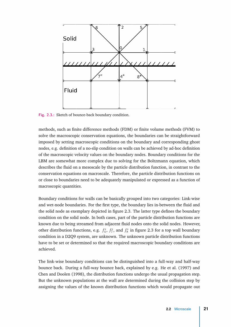
Fig. 2.3.: Sketch of bounce-back boundary condition.

methods, such as finite difference methods (FDM) or finite volume methods (FVM) tosolve the macroscopic conservation equations, the boundaries can be straightforwardimposed by setting macroscopic conditions on the boundary and corresponding ghostnodes, e.g. definition of a no-slip condition on walls can be achieved by ad-hoc definitionof the macroscopic velocity values on the boundary nodes. Boundary conditions for theLBM are somewhat more complex due to solving for the Boltzmann equation, whichdescribes the fluid on a mesoscale by the particle distribution function, in contrast to theconservation equations on macroscale. Therefore, the particle distribution functions onor close to boundaries need to be adequately manipulated or expressed as a function ofmacroscopic quantities.

Boundary conditions for walls can be basically grouped into two categories: Link-wiseand wet-node boundaries. For the first type, the boundary lies in-between the fluid andthe solid node as exemplary depicted in figure 2.3. The latter type defines the boundarycondition on the solid node. In both cases, part of the particle distribution functions areknown due to being streamed from adjacent fluid nodes onto the solid nodes. However,other distribution functions, e.g. f∗4 , f∗7 , and f∗8 in figure 2.3 for a top wall boundarycondition in a D2Q9 system, are unknown. The unknown particle distribution functionshave to be set or determined so that the required macroscopic boundary conditions areachieved.

The link-wise boundary conditions can be distinguished into a full-way and half-waybounce back. During a full-way bounce back, explained by e.g. He et al. (1997) andChen and Doolen (1998), the distribution functions undergo the usual propagation step.But the unknown populations at the wall are determined during the collision step byassigning the values of the known distribution functions which would propagate out

2.2 Microscale 21

of the simulation domain, i.e. f−i = fi where the subscript −i represents the oppositedistribution function of i (e.g. f4 = f2 in a D2Q9 system). For half-way bounce backconditions, the unknown distribution functions at the current collision step are assignedthe values of the opposite particle distribution functions from the previous collision step.Thereafter, the propagation step is performed.

Wet-node boundaries incorporate macroscopic quantities, such as density or velocity, tofind expressions for the particle distribution functions interaction with solid nodes. Acommon wet-node boundary was proposed by Zou and He (1997) who basically evaluatemass and momentum according to ρ =

∑i fi and ρu =

∑fici, respectively, on the

boundary nodes to find expressions for the unknown particle distribution functions. Theresulting system of equations requires however closure which is achieved by assumptionof a non-equilibrium bounce back. Thereby, the unknown particle distribution functionsare expressed in dependence of the known particle distribution function and macroscopicdensities and velocities. The non-equilibrium bounce back boundary can be used to defineeither a velocity or pressure Dirichlet boundary condition. Furthermore, this boundarycondition can be not only used to obtain a no-slip condition on a fixed or moving wall, butcan also be used as an inlet or outlet condition. More wet-node boundary conditions weredeveloped, e.g. Skordos (1993) tries to increase the accuracy by considering fluid velocitygradients in the equilibrium function or Inamuro et al. (1995) who replace the unknownpopulations by an equilibrium function which includes a counter slip velocity to imposethe correct wall velocity. A comparison between common boundary conditions, includingthe aforementioned ones, was conducted by Latt et al. (2008) for boundaries which arealigned to the lattice structure. Latt et al. (2008) found that there is no generally advisedoptimal boundary choice as the choice depends on the simulation geometry and on acompeting influence between stability and accuracy.

Apart from the above described boundary conditions, periodic boundary conditions areeasily implemented in LB simulations. Therefore, the particle distribution functionswhich leave the simulation domain are re-inserted on the opposite simulation domainboundary. Based on periodic boundaries, Wagner and Pagonabarraga (2002) introducedLees-Edwards boundary conditions (LEbc), orignally developed by Lees and Edwards(1972) for molecular dynamic simulations, into the LBM. LEbc allow for study of systemsunder simple shear without any wall influence. The LEbc can be helpful to studyfundamental rheology of suspensions. LEbc are realised by two additional modificationsto the distribution functions which cross periodic boundaries in direction of the shearinggradient: A Galilean velocity transformation and a shift of the particle distributionposition in shearing direction. The Galilean transformation is

fGi (x, t) = fi(x, t) + feqi (x,u + Uboundary, t)− fei q(x,u, t) (2.40)


and the shift in position is

fi(x±, t) = (1− dRx )fGi (x + dIx, t) + dRx fGi (x + dIx ± 1, t) . (2.41)

The shifting procedure of the distribution function has to be interpolated between thediscrete lattice nodes as the resulting shifted position does not necessarily have to lie ona lattice node. Therefore, the shifted distance dx = t∆Uboundary,x is split into an integerdIx and real part 0 ≤ dRx < 1.

Despite the multitude of proposed boundary conditions, the final expressions are relativelysimple and often straightforward to implement. Hence, the LBM is popular for simulationswith complex geometries, such as fluid flows through porous media. E.g. simulationsof flow through static assemblies of particles to obtain precise drag force correlations,which can be then useful for meso- or macro-scale multiphase modelling using CFD-DEMtechniques (cf. Hoef et al. (2005), Beetstra et al. (2007c) and Beetstra et al. (2007a),and references therein).

2.2.3.5. External forcing

In equation (2.31) two terms are found on the right side. The first is a fluid collision term,which was only briefly discussed and more details are given in the next section 2.2.3.6,and the other is a term for consideration of external forces. In the most simple approachintroduced by He et al. (1997), the external force term in Eq. (2.31) is expressed as:

Fi = wiciFc2s

. (2.42)

However, Guo et al. (2002) showed by theoretical analysis that additional error termsappear on the macroscale when an external force as in Eq. (2.42) is included in the LBalgorithm. Guo et al. (2002) suggested modifications to the external forcing so that theimposed external force is expressed as

Fi =(

1− 12τ

)wi

[ci − uc2s

+ (ci · u)c4s

ci]· F (2.43)

and moreover, the velocity calculation is updated to

ρu = ρu∗ + ∆t2 F , (2.44)

where ρu∗ =∑i fici. Thereby, error terms due to external forcing are removed on the

macroscale leading to more accurate results.

2.2 Microscale 23

Another forcing scheme was introduced by Kupershtokh et al. (2009) who wrote theexternal force as

Fi = feqi (u + ∆u)− feqi (u) . (2.45)

The velocity difference in the first equilibrium term is determined from the imposed forceF, i.e. ∆u = F∆t

ρ . The equilibrium velocities are computed according to ρueq =∑i fici

and differ from the real velocities ρu =∑i fici + F∆t

2 . Kupershtokh et al. (2009)introduced this forcing scheme to simulate two fluid flows which interact via an additionalforce term in the LB equation.

In contrast to the above forcing term suggestions, Shan and Chen (1993) set the externalforcing term to Fi = 0 and incorporate forces by modification of the equilibrium velocityin the fluid collision term leading to

ρueq =∑i

fici + Fτρ. (2.46)

Similar to boundary conditions in LB, a variety of suggestions to consider external forcesexist. A review and comparison by theoretical analysis and numerical simulations ofexternal forcing schemes was conducted by Huang et al. (2011). Based on a theoreticalanalysis, Huang et al. (2011) group the various external forcing schemes in two differentgroups depending on similarities in the macroscale error terms. For numerical simulationsof single-phase Taylor-Green vortices, all forcing schemes lead to nearly same accuracies.However, simulations of two-fluid multiphase flow show discrepancies between theforcing schemes of which all obtained results have to some extent a dependency onthe relaxation parameter choice and different accuracies and stabilities are obtained fordifferent schemes, leading to no clear given recommendation by Huang et al. (2011).

2.2.3.6. Collision terms

In section 2.2.3.1, the BGK collision model, Eq. (2.27), introduced into LBM by Qian et al.(1992), is briefly discussed. However, He et al. (1997) showed that the BGK model leadsto slip velocities in Poiseuille flows. The slip velocities are dependent on the relaxationparameter τ , effectively the viscosity, and the employed boundary condition. Yet, theBGK model is only one possible collision term model and other collision models can be aremedy to enforce the no-slip condition for changing viscosities.

As the BGK model has only one relaxation parameter which is linked to the viscosity, in-troduction of multiple relaxation parameters is the logical conclusion. Multiple relaxationtime (MRT) models were introduced by Lallemand and Luo (2000) and D’Humières et al.(2002). The difference to the BGK model is not only the number of relaxation parame-ters, but that rather the moments on macroscale are relaxed instead of the distribution


functions. For that purpose, the particle distribution functions have to be transformedinto the moment space by mk =

∑q−1i=0 Mkifi where Mki is a transformation matrix.

After the collision in moment space, i.e. S[m(x, t)−meq(x, t)] where S = ωiI containsseveral relaxation parameters ωi, a transformation back to the distribution functionspace by multiplication of M−1 has to be performed. The transformation matrix canbe related to different moments by mk =

∑q−1i=0 Mkifi. For example, the first row leads

to m0 = ρ =∑fi =

∑M0ifi → M0i = 1. Some relaxation parameters are related to

physical quantities, shear and bulk viscosity for example, and other relaxation parametersare not and can be therefore freely chosen. The free parameters can be chosen so thata no-slip condition is fulfilled when the viscosity is changed. Moreover, fine tuning ofthe free parameters can lead to increased stability of the simulations, which is especiallyrelevant for high Reynolds number flows.

However, choosing the free relaxation parameters is not straightforward or trivial. Some-what simpler than the MRT scheme is a two relaxation time (TRT) model, suggested byGinzburg (2005), which consists of only two relaxation parameters. One of the relaxationparameters is related to the viscosity and the other parameter can be freely chosen toimprove the accuracy of the simulations.

In both cases, MRT and TRT, the free relaxation parameter(s) have to be determined.For MRT schemes, Lallemand and Luo (2000) and D’Humières et al. (2002) providerelaxation parameter sets based on linear analysis. Another approach is to deriveby theoretical analysis the macroscopic slip velocities for Couette or Poiseuille flowin dependence of the relaxation parameters. Therefore, the velocity momentum iscomputed according to ρu =

∑i fici at the wall in form of a general expression which

includes the relaxation parameters. The obtained expression of the fluid velocity at thewall can be compared to the known analytical solution to obtain an expression for theslip velocity which in turn can be used to find correlations between the freely chosenrelaxation parameters and relaxation parameters which describe physical quantities,such as the viscosity, to improve the no-slip condition. He et al. (1997) found therebyexpressions for the slip velocities in dependency of lattice resolution and single relaxationparameter τ . For immersed boundary methods using TRT or MRT, Lu et al. (2012) andSeta et al. (2014) derived analytically expressions for the free parameters in Coutteand Poiseuille flow. They found by numerical simulations that slip velocities cannot becompletely circumvented, but the improvement in obtained slip velocities is acceptablewhere a TRT scheme can be as effective as a MRT scheme. Alternatively, D’Humièresand Ginzburg (2009) deduced recurrence equations from the LB evolution equationwith a TRT model in steady-state. The recurrence equations are basically a set ofequations which result from a combination of the evaluated LB equation, i.e. all possibleLB propagation steps are written out in explicit forms and combined to recurrenceequations (equations which depend recursively on previous values). The obtained generalrecurrence equations were analysed for bounce-back boundary conditions. D’Humières

2.2 Microscale 25

and Ginzburg (2009) found an optimal combination between the two relaxation timeswhich can lead to reduced constant slip velocities when properly “calibrated” with regardto the employed boundary conditions. Furthermore, free parameters have been attemptedto be empirically determined by conducting simulations and varying the parameters tofind optimal parameters sets with regard to stability and accuracy, e.g. Pan et al. (2004)and Pan et al. (2006). However, the caveat of determining parameter sets for one specificcase, e.g. Poiseuille flow, is the narrow range of its validity. For a changed setup, e.g.coupled fluid-particle flows, a different parameter set might prove more reliable, as statedby D’Humières and Ginzburg (2009), i.e. ideally parameter sets have to be individuallydetermined as they do not apply in general.

2.2.3.7. Fluid-solid couplings

Despite the multitude of boundary conditions in LBM, complex geometries can be simu-lated relatively straightforward, especially when compared to common CFD techniquessuch as FDM or FVM. Thus, LBM is predestined to simulate flow through porous media ormultiphase flow as the bulk of literature in this fields, summarised by Chen and Doolen(1998) and Aidun and Clausen (2010), shows.

Pioneering work to simulate fluid-solid multiphase flow with a LBM was done by Ladd(1994a), Ladd (1994b) and Ladd and Verberg (2001) and has been widely used since then.The coupling between the solid particle and the fluid is based on local momentum transferbetween distribution functions, which are inside and outside the particle volume, on theparticle surface realised by bounce back of the distribution functions. The distributionfunctions colliding with the particle surface are modified by

f−i(x, t+ ∆) = fi(x, t)− 2wiρub · ci (2.47a)

fi(x, t+ ∆) = f−i(x, t) + 2wiρub · ci , (2.47b)

where Eqs. (2.47a) and (2.47b) describe the modifications of the outside and insidedistribution functions, respectively. The opposing distribution function of fi is expressedas f−i and the particle boundary velocity is determined through consideration of trans-lational particle velocity up and angular particle velocity Ωp in relation to the particlecentre of mass xp,c as ub = up + Ωp × (x + 1

2ci − xp,c). The hydrodynamic force andtorque from the fluid on the particle can be computed from the momentum exchangebetween the distribution functions. Therefore, the local forces on the boundary nodes,

FH,LBM,node(x + 12ci) = 2 [fi(x, t)− f−i(x + ci, t)− 2wiρub · ci] ci , (2.48)


have to be summed up: FH =∑FH,LBM,node(x + 1

2ci) and TH =∑

(x + 12ci) ×

FH,LBM,node(x + 12ci). Aidun et al. (1998) removed the fluid within particles to mitigate

the restriction of particles having a much larger density than the fluid and being ableto set the particle density to similar values as the fluid density. However, the fluidremoval within particle volume leads to local violations of the mass conservation. Thebounce back method to couple fluid and solid phase can be used to simulate the rheologyof suspensions in shear flow realised by two parallel sheared wall as was shown byHyväluoma et al. (2005). A simple shear setup between two sheared walls was used byKulkarni and Morris (2008) and Haddadi and Morris (2014) to study the suspensionrheology with regard to viscosity, normal stress differences, pressure, mircostructure,and radial distribution functions. However, for simple shear realised by Lees-Edwardsboundary conditions, Lorenz et al. (2009a) showed that neither the method by Ladd(1994a) nor by Aidun et al. (1998) conserve the particle momentum for a particlecrossing Lees-Edwards boundary conditions. Lorenz et al. (2009a) introduced thereforea correction leading to the correct momentum conservation. Lorenz et al. (2009b)showed that sheared simulations with Lees-Edwards boundary conditions to computebulk viscosities can be possible with the suggested momentum correction.

Another approach to couple fluid-solid flows is the immersed boundary method (IBM)introduced in LBM by Feng and Michaelides (2004) and Feng and Michaelides (2005).Based on the IBM proposed by Peskin (2002), Lagrangian marker points are placed on theparticle surface. The coupling to the fluid, simulated by LBM on an Eulerian backgroundlattice, is achieved by introduction of an additional forcing term Fi in the LB equation:

fi(x + ci∆t, t+ ∆t) = fi(x, t) + Ωfi + Fi . (2.49)

The forcing term is determined from the no-slip condition on the particle surface. There-fore, the fluid velocities have to be interpolated from the Eulerian lattice points xf to theLagrangian marker points xl by

u(xl, t) =∑f

u(xf , t)D(xf − xl)∆x3 , (2.50)

whereD(xf − xl) = δ(xf − xl)δ(yf − yl)δ(zf − zl) (2.51)

and

δ(r) =

14

(1 + cos

(π|r|

2

)), |r| ≤ 2

0 , |r| > 2. (2.52)

The force density at the Lagrangian points G(xl, t),

G(xl, t) = up(xl, t)− u(xl, t)∆t , (2.53)

2.2 Microscale 27

has to be spread to the Eulerian points,

G(xf , t) =N∑l

G(xl, t)D(xf − xl)∆A , (2.54)

where ∆A is the surface area of the corresponding boundary point. The external forcingterm in Eq. (2.49) can be then expressed as:

Fi = 3ρwic2 G · ci . (2.55)

Many different suggestions for combination of fluid collision term and calculation ofthe forcing term have been investigated by Lu et al. (2012) and Seta et al. (2014). Asdescribed in the previous section 2.2.3.6, Seta et al. (2014) found that a TRT schemecan be as effective as a MRT scheme to reduce slip velocity effects. However, the slipvelocities cannot be completely avoided and Seta et al. (2014) show that slip velocitiesdepend not only on the fluid collision scheme, but also on the smoothing function δ whenan IBM is used.

Besides the fluid-solid couplings which are based on the bounce back rule and the IBM,partially saturated cell methods (PSM) can couple fluid and solid phase. As very detailedanalyses of the PSM is performed in chapters 3 and 4, the basic concept is discussedhere only very briefly. In a PSM, developed by Noble and Torcyznski (1998), the particleoverlaps with an Eulerian lattice. Each overlap is considered by a collision term forthe solid phase Ωs

i in addition to the fluid phase collision Ωfi so that the LB equation is

written as:

fi(x + ∆tci, t+ ∆t) = fi(x, t) + [1−B(x, τ)] Ωfi +B(x, τ)Ωs

i , (2.56)

where B(x, τ) is a weighting function to take the particle overlap with the lattice node atx into account. Noble and Torcyznski (1998) suggested two solid phase collision modelsΩsi of which the first, and most popular, is inspired by the non-equilibrium bounce-back

boundary condition,

Ωsi = f−i(x, t)− fi(x, t) + feqi (ρ,Us)− feq−i(ρ,u) , (2.57)

and a second suggestion, named superposition method,

Ωsi = feqi (ρ,Us)− fi(x, t) +

(1− ∆t

τ

) [fi(x, t)− feq−i(ρ,u)

]. (2.58)

Holdych (2003) slightly modified the solid collision term (2.57) by substituting the fluidvelocity by the particle velocity:

Ωsi = f−i(x, t)− fi(x, t) + feqi (ρ,Us)− feq−i(ρ,Us) . (2.59)


Furthermore, the weighting function B(x, τ) can assume different forms. Noble andTorcyznski (1998) proposed a linear weighting function of the lattice solid fraction,

B(x, τ) = εs , (2.60)

and a non-linear function,

B(x, τ) = εs(τ/∆− 1/2)(1− εs) + (τ/∆t− 1/2) . (2.61)

The solid fraction εs on the lattice nodes has to be accurately determined for the PSM.Owen et al. (2011) discuss different approaches to evaluate the solid fraction and groupthem into three different categories, viz. exact closed-form solution, cell decomposition,and polygonal approximation. For the first method, exact closed-form solution, the solidfraction for a lattice node covered by a particle is computed exactly. In contrast, thesecond approach is a brute force method and used in later chapters (cf. also Fig. 3.1).Basically, the lattice cells are decomposed into smaller cells, a subgrid, and the number ofsub-cells inside the particle volume are used to compute the solid fraction. This methodis universally applicable and straightforward to implement, but comes with drasticallyincreasing computational overhead for increasing subgrid resolution. Methods in thethird category evaluate the lattice node solid fraction from polygon (2D) and polyhedra(3D) approximations of the particle surface. In contrast to determining the solid fraction,Zhou et al. (2011) replaced the solid fraction εs in the above weighting functions bya normalised shortest distance Ds, ranging between [0,1], between lattice node andparticle surface, i.e. Ds = 1 − ds

dmaxwhere ds is the shortest distance between lattice

node and particle surface and dmax =√

2/2 is the maximum value of ds (here in a 2Dsystem).

All above described fluid-solid couplings have in common that the Eulerian lattice cellsize is smaller than the particle size, i.e. the fluid flow around the particles is resolvedto a length scale comparable to the lattice cell size. For particles in close contact, whenthe gap distance is below one lattice cell size, the fluid flow cannot be determined.However, for high solid fractions, as for dense suspensions, close range lubrication forcesbetween particles are important. Thus, Nguyen and Ladd (2002) and Ding and Aidun(2003) introduced for small gap distances, which cannot be resolved, a lubrication forcecorrection. Nguyen and Ladd (2002) compute lubrication force corrections on basis of thegrand-resistance matrix (cf. section 2.2.2) which requires only particle properties, suchas particle velocities and sizes, and a gap distance based on the difference between actualparticle gap distances and minimal resolvable gap distance (of the order of one latticecell). In comparison, Ding and Aidun (2003) compute a lubrication force correctionbetween particles for paired lattice nodes (links) whose separation is smaller than theminimal resolvable limit. The total lubrication interaction on a particle is obtained bysummation of corrections applied on all lattice nodes. Although more cumbersome to

2.2 Microscale 29

evaluate, the proposed correction of Ding and Aidun (2003) could be possibly also usedfor non-spherical particles in contrast to the suggestion by Nguyen and Ladd (2002) dueto its formulation being based on the GRM which is only valid for spherical particles.

2.2.4 Navier-Stokes solvers

The simulation of fluid flows has a long history of development efforts and the LBM is arather new technique. In fact, finite difference methods (FDM), finite volume methods(FVM), or finite element method (FEM), which solve for mass conservation and Navier-Stokes equations directly instead of solving the Boltzmann equation, are well establishedand widely used in academia and industry - especially being the standard CFD tool inindustry. Instead of discussing FDM and FVM, a very basic overview of existing fluid-solidcouplings for Navier-Stokes solvers are given here and the interested reader is directedto the extensive and comprehensive discussion on FDM and FVM techniques by Ferzigerand Peric (2002).

Fluid-solid couplings can be classified into two major groups, namely conforming andnon-conforming methods. In conforming methods the numerical mesh conforms tothe particle shape leading to tremendous computational costs for moving particlesdue to frequent mesh movement or remeshing when the numerical mesh becomes tooskewed as shown by Haeri and Shrimpton (2012). In contrast, non-conforming methodsare based on a fixed Eulerian background mesh. Particles overlap with the Eulerianmesh and a coupling between fluid and solid phase is most commonly obtained byuse of an immersed boundary method (IBM), very similar to the IBM discussed in theprevious section 2.2.3.7, or a distributed Lagrange multiplier / fictitious domain method(DLM/FD). A very comprehensive overview of possible IBM and DLM/FD methods isgiven by Haeri and Shrimpton (2012). In essence, coupling of the different phasesis obtained by a no-slip condition on the particle surfaces. Therefore, in the DLM/FDapproach, firstly developed for rigid particles by Glowinski et al. (1998) and Glowinskiet al. (1999), Lagrange marker points are placed over the whole volume of the particlesin contrast to the Lagrange force points distributed only on the particle surfaces in theIBM which was originally developed by Peskin (2002) to simulate blood flow through aheart.

In the DLM/FD framework, a strong and weak coupling can be used. For a strong coupling,a fluid-particle mixture equation in form of a Navier-Stokes equation and a DEM for theparticle phase are solved. The hydrodynamic forces and torques between particles andfluid have to be determined for the strong coupling. In contrast, a weak coupling doesnot require determination of hydrodynamic interactions because the motion equationsfor fluid and particle phase are summarised to a resulting total momentum equationwhich does not contain hydrodynamic force and torque terms. The detailed derivationprocess can be found in Glowinski et al. (1999). Glowinski et al. (1999) show that


the DLM/FD can be used for accurate direct numerical simulations of suspensions byvalidating the method to the settling behaviour of two particles and several hundredcircular discs. The DLM/FD method allows also for simulation of non-spherical particles,e.g. Wachs (2009) simulated sedimentation processes for circular, rectangular, andtriangular particles. Therefore, Wachs (2009) also introduced additionally a soft-spherecontact model capable to model contact forces of arbitrarily convex shaped particles innormal and tangential direction of a collision.

IBMs, as above mentioned, have Lagrangian marker points placed only on the particlesurface. The Navier-Stokes equation for the fluid reads

∂u∂t

+ (u · ∇)u = −1ρ∇p+ ν∇2u + fi , (2.62)

where the term fi represents a force expression between particle i and fluid. A varietyof methods exist to determine the forcing term. In essence, the procedure is similar toIBMs in LBM as discussed in section 2.2.3.7, i.e. the no-slip condition on the particlesurfaces is achieved by interpolating the fluid velocities to the Lagrange force pointsand determining the force term at each Lagrangian point by considering the velocitydifference between fluid and particle surface. The particle velocities are evaluated byNewton’s second law for motion in which also other forces, such as gravitation or collisionforces, can be considered (cf. equations (2.13) and (2.14)). The results for the forcingterm are interpolated back to the Eulerian grid, to be included into the Navier-Stokesequations (2.62). A popular and efficient direct forcing approach for moving particleswas proposed by Uhlmann (2005). According to Uhlmann (2005), a discrete volume isassociated to each Lagrangian force point resulting in a fluid-solid interaction volumeforce term, which is obtained by the aforementioned interpolation procedure, ratherthan a single interaction force acting on each Lagrangian point. Thereby, every particleis surrounded by a layer of volume forces. The proposed method by Uhlmann (2005)leads to smooth particle motions and less restrictive time-step choices. The efficiencyof the IBM is demonstrated, for instance, in direct numerical simulations of turbulentopen channel flows to study sediment erosion effects with over 260000 particles byKidanemariam and Uhlmann (2014).

2.3 Macroscale

2.3.1 Governing equations

Fluid-solid flows can be described on macroscale by an Eulerian-Eulerian approach,such as a two-fluid model (TFM) approach. Both phases, fluid and solid phase, arenot fully resolved continua described by averaged conservation equations. The aver-aged conservation equations (mass, momentum, energy) are deduced for each phase

2.3 Macroscale 31

separately by applying averaging processes (cf. section 2.1.1), such as volume, time-volume and weighted time-volume averaging methods, to the local instantaneous balanceequations.

2.3.1.1. Averaged equations

The derivation of averaged two-fluid equations have been extensively studied by manyresearch groups, e.g. Anderson and Jackson (1967) and Nott et al. (2011). The final setof averaged two-fluid equations for a single fluid and single solid phase, whose stepwisededuction can be found for example in Anderson and Jackson (1967), are obtainedby applying a weighted averaging technique, such as Eq. (2.5), on point mass andmomentum conservation equations and can be written with an external volume force(e.g. gravity) ρg as:

∂ε

∂t+∇ · (〈εuf 〉) = 0 , (2.63)

for the averaged fluid mass conservation and

ερf

[∂

∂t(〈uf 〉) + (〈uf 〉 · ∇)〈uf 〉

]= ∇ · 〈σf 〉 − Ffp + ερfg , (2.64)

for the averaged fluid momentum conservation. Similar averaged equations are foundfor the solid phase. The averaged mass conservation equation for the solid phase is

∂φ

∂t+∇ · (〈φus〉) = 0 , (2.65)

and the averaged momentum conservation equation for the solid phase reads

φρs

[∂

∂t(〈us〉) + (〈us〉 · ∇)〈us〉

]= −∇ · 〈σs〉+ Ffp + Fss + φρsg . (2.66)

Each phase has its own velocity, uf and us, which is weighted by porosity ε and solidfraction φ = ε− 1 for the fluid and solid phase, respectively. The momentum equationscontain furthermore separate stress tensors for fluid and solid phase, σf and σs, whichrequire adequate modelling which is discussed in subsequent sections. Moreover, in-teraction between the fluid and solid phase is considered by the interaction force termFfp and similarly interactions between different solid phases can be considered by asolid-solid interaction term Fss.

Very similar to the above TFM, the suspension balance model (SBM) describes thesuspension behaviour on macroscale by mass and momentum conservation equationsfor fluid, particle, and suspension mixture. The main difference is consideration ofparticle migration due to stress gradients in the SBM. Two of the three phase equations(fluid,particle, suspension mixture) are necessary to evaluate and according to Nott et al.


(2011), the suspension momentum and particle momentum balance equations withparticle volume Vp and particle number per volume element n can be written as

∂

∂t〈ρu〉+ ∇ · 〈ρuu〉 = ∇ · [ε〈σf 〉+ φ〈σs〉] + 〈F〉 (2.67)

andρpVp

[∂

∂t(n〈up〉) + ∇ · (n〈upup〉)

]= nVp〈Fext,p〉+ n〈Fp〉 , (2.68)

respectively. Fext,p is an external force term, such as gravity, and Fp is the particle phaseforce, which can include terms such as the drag force or force terms due to hydrodynamicstress. The force term F in Eq. (2.67) is a net body force and for example, consists agravity and interphase force. The corresponding mass conservation equations read forthe suspension

∇ · 〈u〉 = 0 (2.69)

and for the particle phase∂φ

∂t+ ∇ · 〈φup〉 = 0 . (2.70)

2.3.1.2. Closure laws

The obtained averaged set of equations require closures. Enwald et al. (1996) elucidatethat three types of closure are necessary, viz. topological, constitutive and transferclosures. Topological closures are needed for description of spatial distribution of flowvariables. Physical properties for each phase are covered in corresponding constitutiveclosures and interactions between the phases, such as drag, lift, or buoyancy forces, aresummarised in transfer closures.

2.3.2 Transfer closures

The fluid-particle interaction force Ffp is, in contrast to microscale simulations, volumeaveraged over single fluid-particle forces Ffp = 1

V

∑ffi (cf. Hoef et al. (2008), Xiao and

Sun (2011)) and consists of several different parts: Buoyancy force, drag force, Bassetforce, lift force, Saffmann force, and Magnus force. Considering only buoyancy and dragforce Fip,d, the fluid-particle interaction force is

Fip = −φ∇p+ Fip,d , (2.71)

where Fip,d = β(uf − us) is the drag force connecting the relative velocity between fluidand solid phase through an interphase momentum transfer coefficient, or sometimes alsocalled friction coefficient, β.

2.3 Macroscale 33

The simplest drag correlation is the Stokes drag force, which is valid for a single spherein a low Reynolds number flow, and it follows for the inter-phase momentum exchangecoefficient:

β = 6πηfrp . (2.72)

2.3.2.1. Monodisperse drag models

A common drag force modelling approach is based on the results of Ergun (1952).Ergun determined the pressure drop of a flow through a static assembly of spheres andthereby obtained an expression for the drag force valid for dense particle systems. Formonodisperse dilute systems, Wen and Yu (1966) proposed a drag model. Commonly,both drag models by Ergun (1952) and Wen and Yu (1966) are combined to capture thevast range of solid fractions in monodisperse systems, i.e.:

β =

150φ2

εηfd2p

+ 1.75φρfdp |uf − us| , φ ≥ 0.234Cd

εφdpρf |uf − us|ε−2.65 , φ < 0.2

. (2.73a)

CD(Re) = 24

Re(1 + 0.15Re0.687) , Re < 10000.44 , Re ≥ 1000

. (2.73b)

Re = ερf |uf − us|dpηf

(2.73c)

However, the transition in force between the dense and dilute system is not smoothwhich is shown by Beetstra et al. (2007c).

Similar studies of flow through static assemblies of particles to obtain drag force correla-tions, however on numerical basis, were conducted, e.g. by Hill et al. (2001), Benyahiaet al. (2006), Hoef et al. (2005) and Beetstra et al. (2007a). Hill et al. (2001) derived adrag model for solid fractions ranging close to the maximum packing fraction of staticmonodisperse particle assemblies and for Reynolds number to the order of Re ≈ O(100).The model was extended for void fractions and Reynolds numbers, which are typicallyfound in fluidised beds, by Benyahia et al. (2006). Hoef et al. (2005) and Beetstra et al.(2007a) extended drag correlations to larger Reynolds numbers and considered moreoverbidisperse particles (cf. next section).

Drag models can be also deduced by studying the sedimentation of particles. Thereby,Syamlal et al. (1993) derived a popular drag model.


Di Felice (1994) found a way to express the drag force on multiple particles by multiplyingthe drag force of a single particle with a voidage function to consider influences ofneighbouring particles.

The aforementioned models are appropriate for only specific applications. Considerationof further influential parameters (e.g. polydisperse particles, non-spherical particles,segregation processes, aggregation and breakage processes, heat transfer) requiresmodifications and extensions of existing models as well as calibration of correspondingmodelling parameters or development of a complete new model.

2.3.2.2. Polydisperse drag models

LBDEM simulations of flow through static mono- and bidisperse particle assembliesfor solid fractions ranging to close-packing of the assemblies, i.e. φmax ≥ 0.6, wereconducted by Hoef et al. (2005) for low-Reynolds number flows, Re << 1, and byBeetstra et al. (2007a) who extended the investigated Reynolds number regime to theorder of Re ≈ O(1000). Large deviations between monodisperse drag force expressionsand actual drag forces in bidisperse systems are found. The obtained LBDEM dataresulted in the construction of an improved drag model for bidisperse system. Thenewly derived (and corrected; cf. Beetstra et al. (2007b)) drag model is based on amonodisperse drag model extended by a correction factor to incorporate the bidispersityand can be written in the simplest case in dimensionless form as follows:

Fip,d = (εyi + (1− ε)y2i )Fip,d,mono(ε, 〈Re〉) , (2.74)

where Fip,d,mono(ε, 〈Re〉) is the corresponding monodisperse drag force for the sameporosity as in the polydisperse case. The model parameters are defined as yi = di

〈d〉 ,

〈Re〉 = ρFU〈d〉ηf

and 1〈d〉 =

∑iκidi

. Furthermore it is demonstrated that bidisperse dragforce modelling is crucial because of high deviations between bidisperse simulationresults and the monodisperse drag force models. For higher packing fractions φ > 0.5,Beetstra et al. (2007a) conclude that the particle assembly indicates some ordering.Therefore, the drag force is dependent on the flow direction for large Reynolds numbersand thus, data was averaged over simulations with different directions.

Sarkar et al. (2009) investigated by LBDEM simulations fluid flow through fixed polydis-perse particle assemblies. Two types of random particle assemblies were investigated:Gaussian and log-normal size distribution. It is found that the influence of the differentsize distributions on the drag force can be neglected.

2.3 Macroscale 35

2.3.2.3. Particle-particle drag

Particles in a suspension affect each other in its motion by transmitting forces through thefluid due to sheer presence or relative velocities. Therefore, Yin and Sundaresan (2009a)studied equally sized particle assemblies with two different imposed velocity values ontwo types of particles in a low Reynolds number and high Stokes number regime. On thisbasis, Yin and Sundaresan (2009a) introduced, similar to the grand-resistance matrixnotation for particle-particle lubrication forces, a particle-particle drag law for particleswith relative velocities to each other:

Fip,d =

Fip,d1 = −B11∆U1 −B12∆U2

Fip,d2 = −B21∆U1 −B22∆U2, (2.75)

where the particle-specific friction coefficients Bij are determined from simulations.Lubrication forces between particles affect the hydrodynamic particle-particle drag andYin and Sundaresan (2009a) elucidate that the particle-particle drag influence on fluid-particle drag can be important. Therefore, Yin and Sundaresan (2009a) compared theirdrag law to the combined drag correlation given in equations (2.73) and found thatparticle-particle drag is important to be considered and it could have a large influenceon simulations of segregation phenomena. Extension of the particle-particle drag lawtowards particles of different sizes was undertaken by Yin and Sundaresan (2009b) andmodification to include inertial effects due to higher Reynolds numbers were consideredby Holloway et al. (2010).

2.3.3 Constitutive closures

Evaluation of the above described TFM and SBM require also closure expressions for theunknown stress terms for the fluid phase σf and solid phase σs, i.e. constitutive closures.Closures for the stress terms are of paramount importance because the whole physicalbehaviour of one phase is mirrored in the stress closures.

2.3.3.1. Suspension stress - theory

An approach for suspensions to relate the microscale to macroscale was proposed byBatchelor (1970) who derived a general formulation for the computation of bulk stressin a suspension. According to Batchelor (1970), the bulk stress can be computed as:

Σij = 1V

∫(σij − ρu

′iu

′j)dV (2.76)


where V is the averaging volume. For an incompressible Newtonian fluid, equation(2.76) can be written as:

Σij = 1V

∫V−∑

Vp

[−pfδij + ηf

(∂ui∂xj

+ ∂uj∂xi

)]dV + 1

V

∑∫VpσijdV −

1V

∫ρu

′iu

′jdV ,

(2.77)where Vp is the particle volume. The first integral on the right-hand side represents theNewtonian fluid stress which is split into a pressure pf and viscous stress contribution.The two last terms are commonly described as the “particle stress”

∑pij:

Σpij = 1

V

∑∫VpσijdV −

1V

∫ρu

′iu

′jdV (2.78)

where the first term is the stress inside the particle volumes and the second term is astress contribution stemming from the particle velocity fluctuations u

′. Application of the

divergence theorem leads to:

1V

∑∫VpσijdV = 1

V

∑∫ApxjσiknkdA−

1Vp

∫∂σij∂xj

xjdV (2.79)

and with the particle acceleration a(r) = a +α× r+ω× (ω× r) at position r (r pointingfrom centre of mass to the point r) inside of a particle for ∂σij

∂xj= ρai where the constant

fluid density is ρ is uniform in space, the particle stress reads:

Σpij = 1

V

∑∫ApxjσiknkdA−

1V

∑∫VpρxjaidV −

1V

∫ρu

′iu

′jdV . (2.80)

The first term on the right-hand side is the stresslet, the second term the accelerationstress and the last term is the Reynolds stress. The stresslet can be computed as

σstressletij = 1V

∑∫ApxjσiknkdA = 1

V

∑∫Ap

12(σikxj + σjkxi)nkdA , (2.81)

the acceleration stress as

σaccelerationij = 1V

∑∫VpρxjaidV = 1

V

∑∫Vp

(12(aixj + ajxi)

)dV , (2.82)

and the Reynolds stress as

σReynoldsij = 1V

∫ρu

′iu

′jdV = 1

V

∑i

miu′iu

′j . (2.83)

2.3 Macroscale 37

Similar to Batchelor (1970), Nott et al. (2011) decomposed the bulk stress into a fluidand particle contribution in the suspension momentum equation (2.67). The fluid stressfor an incompressible Newtonian fluid with rigid particles is

ε〈σf 〉 =∫Vf

(−pI + 2ηfe)dV = −ε〈pf 〉I + 2ηf 〈e〉 . (2.84)

The stress for the solid phase is according to Nott et al. (2011):

φ〈σs〉 =∑i

gi

∫Vp,i

σdV −∇ ·∑i

gi

∫Vp,i

y′σdV + ... , (2.85)

where gi is a weighting function at the centre of particle iwith the property∫gdV = 1 and

y′ = y− yi with y being an unaveraged coordinate over space. Further simplifications,discussed by Nott et al. (2011), lead ultimately to:

φ〈σ〉s =∑i

gi

(Si −

12ε ·Ti +

∫Vp,i

y′F′dV

)

− 12∇ ·

∑i

gi

(Qi −

15Vpd

2pIf i +

∫Vp,i

y′y′F′dV

)+ ... , (2.86)

where f i =∫S,i n · σdS is the zeroth moment of surface traction, Si = 1

2(Si + STi ) is thefirst moment of the surface traction where Si =

∫S,i y

′n ·σdS, Qi =∫S,i y

′y′n ·σdS is thesecond moment of surface traction, F′

is the deviation of the mean of F, and Ti is theexternal torque on particle i with ε being the Levi-Cita symbol. Although the result is verysimilar to Batchelor (1970), especially when gi = 1

V is chosen, a main difference in termsof an additional gradient, including a second moment of the surface traction, is obtained.The found additional terms are only observable for suspensions with a non-uniform stressstate in the stress tensor elements as the gradients otherwise disappear.

2.3.3.2. Bulk stress and viscosity computation in simulations

The bulk stress contributions can be computed based on the theoretical work discussedin the previous section.

2.3.3.2.1. Stress for interparticle forces from DEM For incompressible rigid particles,the mean stress within a solid is not affected by the elastic properties and the stress canbe straightforward computed from the interaction force on the corresponding interactionsurface point. In case of interparticle forces, the stresslet computation can be performedaccording to Thompson et al. (2009), which is in accordance with Nott et al. (2011), forthe contact force

σC = 1V

∑i

∑j

rijFCij (2.87)


and pair-wise lubrication forces

σL = 1V

∑i

∑j

rijFLij . (2.88)

2.3.3.2.2. Stress for fluid-solid interaction from LBM In case of non-interparticle forces,such as drag forces, computed in LBM simulations, the bulk stress can be computed bydifferent approaches. Haddadi and Morris (2014) re-write the stresslet (2.81) to:

1V

∑∫Ap

12(σikxj + σjkxi)nkdA = 1

V

Nparticles∑ Nnodes∑(12(fLBMik xj + fLBMjk xi)) , (2.89)

where the hydrodynamic force fLBM on each particle covered lattice node is summedfor the corresponding particle to obtain the particle stress value.

Krüger et al. (2011) compute for a LBM-IBM the particle stress contribution by relatingthe hydrodynamic lattice node force Fjx, where x is the shearing direction, to a planewhich slices the simulation domain at position z, where z is the direction of the shearinggradient, i.e.:

Σpxz(z, t) = 1

2A∑j

Fjx(t)sgn(z − Zj) . (2.90)

A is the surface of the intersecting plane at location z and Zj is the lattice node coordinatein z direction at which the force Fjx is evaluated.

A more cumbersome stress computation is used by Shakib-Manesh et al. (2002) andHyväluoma et al. (2005) who use the fluid-solid coupling proposed by Ladd (1994a)and Ladd (1994b). The hydrodynamic shear stress contribution τfp is computed fromthe spatial, time, and ensemble averaged fluid-particle force in shearing direction Ffp.Therefore, Ffp is related to an intersecting surface Ap between particle volume anda plane Sp slicing the simulation domain with its normal component parallel to theshearing gradient:

τfp = 〈FfpAp〉 . (2.91)

The fluid-particle force Ffp is determined for the particle volume above or below theintersecting plane Sp and reads exemplary for the lower intersected particle volumeFfp = −Fi,d−Fo,d+mda+mdα×rd+mdω

2rdey. The first two terms are hydrodynamicforces acting on the particle from inside the particle and outside the particle. The lastterms are related to the particle acceleration a and particle rotations with angular velocityω. rd is the vector from particle centre to the centre-of mass of the particle volume belowthe intersecting plane Sp with the corresponding mass md.

2.3 Macroscale 39

2.3.3.2.3. Viscosity computation The viscosity of a suspension can be determined bysumming the different stress computations, discussed in the previous sections, andrelating the total bulk stress to the shear rate γ, i.e.

η = ηf +Σpxy

γ, (2.92)

where∑pxy = σC + σL + σstresslet + σacceleration + σReynolds with contributions from the

above equations.

Alternatively, the viscosity can be also determined from the dissipation in the shearedsystem. In molecular dynamic simulations, Andreotti et al. (2012) determine the viscosityby evaluation of

η = Γγ1+νbf , (2.93)

where Γ is the dissipation which is computed from viscous forces and particle velocityfluctuations as

Γ = 1V

[∑i

Fvisci · [up,i − uflow(xp,i)]

]. (2.94)

Without providing here the details of the viscous force expression used by Andreotti et al.(2012), it shall be only remarked that the parameter νbf is part of the viscous force Fvisc

and describes the background fluid as Newtonian νbf = 1 or non-Newtonian νbf 6= 1.

According to Lishchuk et al. (2006) the dissipation in LBM simulations is

Γ = ηf2∑V

(∂uα∂xβ

+ ∂uβ∂xα

)2V,t

, (2.95)

where lattice nodes within particle volume are excluded in the volume V and velocitygradients can be evaluated by ∂uα

∂xβ= 1

c2s

∑iwiuα(r + ci)ciβ + O(c3

i ). The suspensionviscosity η is then found by the relationship η = Γtot

γ/2 where Γtot is the total dissipation inthe system and γ is the imposed shear rate on the system.

2.3.3.3. Dimensional analysis of suspension systems

In the previous sections, it has been shown which microscale occurrences contributeto the overall suspension bulk stress and how these contributions can be calculated insimulations. However, development of constitutive models to find closures for the stressterm can be simplified when the focus is set on specific flow regimes or parameter sets.Therefore, a simple sheared suspension system with its characteristic parameters is herediscussed first to show basic rheology determining parameters in form of dimensionless


ρf ρp γ ηf di ci σ Vp µr fh kn

M 1 1 0 1 0 0 1 0 - 0 1L -3 -3 0 -1 1 1 -1 3 - 1 0T 0 0 -1 -1 0 0 -2 0 - -2 -2

Tab. 2.1.: Buckingham matrix for a suspension

numbers. A comparison to dimensionless numbers in the literature is finally undertakenbefore the focus is shifted to constitutive modelling in the next section 2.3.3.4.

Fig. 2.4.: Sheared suspensions system

2.3.3.3.1. Buckingham analysis On the most fundamental level, a suspension can bestudied under simple shear as depicted in figure 2.4. The suspension consists here ofan incompressible Newtonian fluid of density ρf and dynamic viscosity ηf with rigidparticles of density ρp, diameters di, and elastic stiffness kn. Lubrication interactionsbetween particles can occur for gap distances which are comparable in size of particlesurface roughnesses and therefore, an inner cut-off distance ci can be defined. Frictionbetween particles is considered by a coefficient of friction µr and interaction betweenfluid and particles by a hydrodynamic volume force fh, as in the above TFM. The wholesuspension of fluid and N particles is sheared with a shear rate of γ = 2U

H leading to asuspension stress σ. All parameters are summarised in a Buckingham matrix presented intable 2.1 which has the rank r = 3 with at least n = 10 parameters, i.e. leading to at least7 dimensionless numbers. Simplifications can be undertaken by assuming a bidispersesystem with a fixed particle diameter ratio so that d = didj

di+dj can be used to substitute the

2.3 Macroscale 41

various particle diameters di in table 2.1. Dimensionless numbers with γ, d and ηf as thebasis read then:

π1 = ρfηfγd2

= Re , (2.96a)

π2 = ρpηfγd2

= St , (2.96b)

π3 = cid, (2.96c)

π4 = Vp

(Hd d)3 = φ , (2.96d)

π5 = µr , (2.96e)

π6 = fhd

d2γ2 = fhd

U20

= 1Fr2 , (2.96f)

π7 = knηf γd

= k∗n . (2.96g)

π8 = σ

ηf γ. (2.96h)

The characteristic velocity is here defined to be U0 = dγ to make the connection betweenhydrodynamic force and commonly known Fr number, which represents the ratio be-tween fluid inertial forces and body forces, apparent. Constitutive models for suspensionsare constructed to find adequate closure expression for the stresses σ, i.e. of interest isthe determination of a functional π8 = f(π1, π2, π3, π4, π5, π6, π7) or

σ

ηf γ= f(Re, St, ci

d, φ, µr, F r, k

∗n) . (2.97)

The Stokes number and Reynolds number, which gives the ratio between fluid inertialforces and viscous forces, can be linked to each other by

St = ρpd2γ

ηf

ρfρf

= ρpρfRe . (2.98)

Under the assumption of ρf = ρp = ρ, i.e. for neutrally buoyant suspended particles, theStokes number and Reynolds number are identical.

2.3.3.3.2. Comparison to literature Ancey et al. (1999) discuss a few dimensionlessnumbers to characterise fluid-solid flows and classify suspension regimes. The Stokesnumber St is a common characterisation giving the ratio of a particle inertia responsetime to a fluid convective time. Therefore, the Stokes number characterises the couplingbetween particle motion and fluid, i.e. St << 1 results in the fluid predominating and


hence the particle following the fluid flow, whereas on the contrary, independent particlemotion from the fluid occurs for St >> 1. The Stokes number is expressed by Anceyet al. (1999) as:

St =ρpr

2pγ

ηf, (2.99)

which is virtually identical to the Stokes number St = ρpηf

γd2found by the Buckingham

analysis in the previous section 2.3.3.3.1 except for the scaling with the particle radius rp.Similarly to the Buckingham analysis above, Haddadi and Morris (2014) use a a virtuallyidentical Reynolds number formulation (radius instead of diameter) and link in the verysame way as in Eq. (2.98) the Stokes number with the Reynolds number.

According to Ancey et al. (1999), main suspension regimes can be classified with threedimensionless number which are obtained from setting different force contributionsratios, viz. the Bagnold number Ba, the Coulomb number Co and the Leighton numberLe. The Bagnold number,

Ba = 1ln(co/ci)

ρpr2pγ

ηf, (2.100)

describes the ratio of particle inertia to the work of normal lubrication forces.

The second dimensionless number, the Coulomb number,

Co =ρpr

2pγ

2

Σp, (2.101)

represents the ratio of collisional to frictional contacts where Σp is the particle stress.

The Leighton number,

Le = ηfrpγ

ciΣp, (2.102)

describes the ratio of frictional and lubrication forces. Ancey et al. (1999) show that theLeighton number is not independent of the Coulomb and Bagnold number, i.e. Le ≈ Corp

ciBa.

Based on the Bagnold, Coulomb, and Leighton number, Ancey et al. (1999) differentiatethe suspension rheology into three regimes: Frictional regime (Co << 1 and Le << 1),collisional regime (Co >> 1 and Ba >> 1), and hydrodynamic regime (Ba << 1 andLe >> 1).

If additionally the thermal energy kBT is considered, where kB is the Boltzmann constantand T is the temperature, another dimensionless number, the Peclet number, is found,e.g. Stickel and Powell (2005):

Pe =6πηfr3

pγ

kBT. (2.103)

2.3 Macroscale 43

The Peclet number is useful to classify between Brownian and non-Brownian regimes(Pe→∞). Moreover, Stickel and Powell (2005) show that depending on the Reynoldsand Peclet number combination the rheological behaviour can be classified into Newto-nian, shear-thinning, and shear-thickening regimes.

An additional important dimensionless number for dry granular media, which sets particleinertia in relation to confining stress, is given by Midi (2004):

I = γd√p/ρp

, (2.104)

where p is the confining pressure of the system. The inertial number I, giving the ratio ofinertial time of particle rearrangement on microscale to time of strain (macroscale), ishowever not valid for low Stokes numbers and systems should be described by a viscousnumber according to Cassar et al. (2005) or Boyer et al. (2011):

Iv = ηf γ

p. (2.105)

2.3.3.3.3. Conclusion of dimensional analysis The dimensionless numbers Le,Ba,Coare not independent to each other as shown by Ancey et al. (1999). Furthermore, Stokesnumber St and Bagnold number Ba are extremely similar. Moreover, Leighton numberLe and viscous number Iv differ effectively only in the considered stress - particle stressor pressure. However, the dimensionless suspension stress is expressed as Buckinghamfunctional. Hence in summary, taking all the previously elucidated dimensionless numbersand relations into account, the suspension stress might be generally expressed as thefollowing functional:

σ

µγ= f(Re, St, ci

d, φ, µr, F r, k

∗n, P e, Iv) . (2.106)

However, the dimensionless parameter list (2.106) is not extensive as many more param-eters can, and should be, considered - particle size distributions, particle shape, particledeformability, cohesive forces, and turbulence to name but a few.

2.3.3.4. Constitutive equations

In section 2.3.3.1, the bulk stress is decomposed into a fluid and solid contribution. It isexplained that the fluid bulk stress can be further decomposed into a pressure pf andviscous stress τ f contribution:

σf = −pfI + τ f . (2.107)


where I is the identity tensor. For an incompressible Newtonian fluid the shear stress canbe expressed as

τ fαβ = ηf

∂ufα∂xfβ

+∂ufβ

∂xfα

. (2.108)

On this basis, the stress tensor for the solid phase could be analogously decomposed intoan inter-particle pressure ps and a solid shear stress component τ s

σs = −psI + τ s , (2.109)

where the solid shear stress could be modelled similar to a Newtonian fluid, i.e.

τ sαβ = ηs

(∂usα∂usβ

+∂usβ∂xsα

). (2.110)

However, in contrast to a Newtonian fluid, the solid phase pressure ps is not isotropic andthe viscosity ηs can be a complex function depending on the dimensionless parametersdiscussed in the previous section.

The suspension viscosity increases with increasing solid fraction. Einstein (1905) derivedfor very dilute suspension the relative viscosity ηr = ηsuspension

ηfrelation

ηr = 1 + φ (2.111)

and Einstein (1911) published later an erratum to correct his derivation to

ηr = 1 + 2.5φ . (2.112)

Batchelor and Green (1972a) extended the solution to a higher order, i.e.

ηr = 1 + 2.5φ+ 7.6φ2 . (2.113)

However, for a further increase of the solid fraction the analytical solutions differ tremen-dously from experimental findings. Eilers (1941) compared different formulas to de-termine the viscosity for any given solid fractions and concluded with the suggestion

ηr =

1 + 2.5φ2(1− φ

0.74

)2

, (2.114)

where the expression in the numerator stems from the above Einstein correlation fordilute suspensions and the factor 0.74 in the denominator corresponded to a specific

2.3 Macroscale 45

maximum packing fraction in the system. Therefore, the correlation by Eilers (1941) isoften generally expressed as

ηr =

1 + [η]φ2(1− φ

φmax

)2

, (2.115)

where [η] is called an intrinsic viscosity, e.g. by Krieger and Dougherty (1959), andserves with the maximum packing fraction φmax as fitting parameters. An alternativepopular correlation between solid fraction and viscosity was semi-empirically determinedby Krieger and Dougherty (1959):

ηr =(

1− φ

φmax

)−[η]φmax, (2.116)

where φmax is a close packing fraction depending particle phase properties and [η] is anintrinsic viscosity which depends on the suspension properties and is according to Kriegerand Dougherty (1959) around [η] = 2.5. Although the above correlations are a functionof the solid fraction, Jeffrey and Acrivos (1976) state after comparison of differentexperimental investigations that not only the solid fractions, but also other parameters,such as particle shape or particle size distributions, are important to consider.

As mentioned in the previous section 2.3.3.3.2, Midi (2004) found a dimensionlessnumber, the inertial number I (2.104), to characterise granular flows and constructconstitutive models. Therefore, the shear stress τ and solid fraction φ depends on theinertial number, i.e.

τ = µeff (I)ps (2.117a)

φ = φ(I) , (2.117b)

where ps is the particle pressure in the system and µeff is the effective friction coefficientand depends on the inertial number (2.104). Cassar et al. (2005) investigated submarinegranular flows and accounting for the particle surrounding fluid, modified the inertialnumber for use in different flow regimes, such as viscous, inertial, or free fall regime.Boyer et al. (2011) used the modified inertial number for the viscous regime, the viscousnumber Iv by Cassar et al. (2005), to develop a constitutive modelling approach forsuspensions which is similar to the constitutive models suggested by Midi (2004) for“dry” granular materials. The shear stress τ and particle pressure ps in a suspension arethen expressed as

τ = ηs(φ)ηf γ (2.118a)


ps = ηn(φ)ηf γ . (2.118b)

The effective shear and normal viscosities, ηs and ηn, respectively, are found by compari-son of equations (2.118) with the viscous number (2.105) for the particle pressure andwith equation (2.117) for the shear stress so that it follows:

ηs(φ) = µ[Iv(φ)]Iv(φ) (2.119a)

ηn(φ) = 1Iv(φ) . (2.119b)

Boyer et al. (2011) suggest for modelling of µeff a combination of a contact contribution,which is similar to findings in “dry” granular materials, and a hydrodynamic part. Insteadof giving the lengthy effective friction coefficient model and final viscosity expressionshere, the reader is advised to consult the publication by Boyer et al. (2011). Furtherwork, based on the Iv-modelling approach was performed by Ness and Sun (2015) whopropose a constitutive model covering various suspension flow regimes by linking to a“dry” granular model proposed by Chialvo et al. (2012).

2.3 Macroscale 47

3An analysis of two lattice Boltzmannpartially saturated cell methods tosimulate suspensions of solidparticles

3.1 Introduction

Previous chapters elucidate that simulations can be employed to study in detail fluid-particle flows and various methodologies have been developed in the past. Methodsfor popular (and classic) finite difference (FDM) or finite volume methods (FVM) weredeveloped, e.g. by Glowinski et al. (1999), Peskin (2002), Uhlmann (2005). However,computationally advantageous to FDM/FVM is the lattice Boltzmann method and differ-ent fluid-solid LBM coupling approaches, briefly discussed in a previous section 2.2.3.7,were proposed. One of the earliest and most used coupling approaches was developedby Ladd (1994a) and Ladd (1994b) which is based on a simple bounce back boundarycondition on the particle surface. Improvements with regard to the momentum exchangewere suggested by Aidun and Lu (1995) and Aidun et al. (1998). Nguyen and Ladd(2002) introduced explicit lubrication force corrections. Similar to the aforementionedFDM/FVM coupling approaches, also an immersed boundary method was developed forthe LBM by Feng and Michaelides (2005).

An alternative approach, which is investigated with its applicability to suspension simula-tions in this thesis, was proposed by Noble and Torcyznski (1998) who extended the LBMby an additional collision term for the solid phase. The fluid and solid collision terms areappropriately weighted with a solid fraction weighting function describing the overlapsbetween lattice nodes and particle. Noble and Torcyznski (1998) proposed two differentmodelling approaches for the solid phase collision term, viz. a suggestion based on thenon-equilibrium bounce back and a second suggestion described as superposition method.In general, the advantage of the partially saturated cell method (PSM) is its simplicitywhich conserves the locality of LB node computations. Hence, several studies showed inthe past its validity for many different cases. Verification and validation with regard to thehydrodynamic force and torque calculations for particles were for example performed byOwen et al. (2011) and Seil (2016). Owen et al. (2011) simulated therefore various casesin 2D and 3D to assess the PSM. 2D simulations comprised flow around a cylinder as

49

well as a rectangular box for different Reynolds numbers, 0.5 ≤ Re ≤ 40, and simulationsresults were compared to experimental and simulation results in the literature. For thecylinder, the obtained drag coefficient corresponds well to experimental findings forthe investigated Reynolds number range except for low Reynolds numbers Re ≤ 1. Incontrast, the drag coefficient for the rectangular box was found to agree well for thewhole investigated Reynolds number range. However, some small differences are foundfor the recirculation length of the fluid flow behind the rectangular box as well as in thetransitions to symmetric flow vortices and unsteady wake behind the box compared toFVM and LBM simulation results from the literature. An additional 2D verification andvalidation case was performed by studying Couette flow realised by a rotating cylinderwithin larger hollow cylinder. Owen et al. (2011) show that the non-equilibrium bounceback method and the superposition method for the PSM can capture the developedvelocity profile in the cylindrical Couette flow. The obtained torque has been shown tobe more accurate for the non-equilibrium bounce back method, yet the error for themaximum velocity at the rotating cylinder surface is much smaller for the superpositionmethod showing a contrasting accuracy behaviour. Cook et al. (2004b) performed verysimilar cylindrical Couette validation cases for the PSM, but only for the non-equilibriumbounce back method, which lead to comparable results to Owen et al. (2011). Furthervalidation was undertaken by Owen et al. (2011) in 3D by simulating flow through aperiodic array of a sphere, flow around a single sphere, and multiple particles settling ina fluid with the non-equilibrium bounce back method. The results for the former twocases agree with findings in the literature, but also show that the PSM is seemingly moreaccurate towards higher Reynolds numbers. For the latter multi-particle case, typicalvortex structures are found which indicates the methodology’s capability to simulatefluid-solid flows. Very similar verification and validation cases were carried out by Seil(2016) whose open-source coupling between the Palabos (LBM) and LIGGGHTS (DEM)solvers is used in this thesis with some minor modifications relevant to dense suspensions(e.g. particles overlapping on a same lattice node). Seil (2016) shows as well in 2D thatthe PSM can lead to correct drag coefficients for flows around single fixed spheres ortorque calculations in cylindrical Couette flows as described above. In 3D, Seil (2016)conducted simulations of a fixed sphere in sheared channel showing that drag, lift, andtorque values are in agreement with results obtained from FVM simulations carried outwith the commercial FLUENT code. Further 3D validation was performed by studyingthe settling behaviour of a single sphere in a closed container for different Reynoldsnumbers. Simulation results were compared to experimental findings in the literatureand a good agreement is found for higher Reynolds numbers. But growing discrepanciesare observed for decreasing Reynolds numbers, especially in the wall region beforeparticle-wall collision.

A slight modification to the non-equilibrium bounce back solid phase collision term,cited frequently in the literature, was proposed by Holdych (2003). Holdych (2003)modified the non-equilibrium bounce back solid phase collision term by substitution

50 Chapter 3 An analysis of two lattice Boltzmann partially saturated cell methods

of the fluid velocity by the solid phase velocity to analyse momentum truncation errorterms for one-dimensional steady flow for a fixed relaxation parameter τ = 1.0 underthe assumptions of a uniform solid velocity distribution and no-slip on the fluid-solidinterface. However, numerical instability problems and non-convergence problems in twodimensional simulations are reported by Cook et al. (2004a) and by Wang et al. (2016),respectively. Moreover, Leonardi et al. (2016) state that the proposed modification byHoldych (2003) is only applicable for stationary particles. Strack and Cook (2007)contradict those findings by reporting of validation cases which include besides fixedspheres, freely settling particles for varied Reynolds numbers and simulations of the draft-kissing-tumbling case for two particles in 3D. Yet, instability problems in 3D-simulationsfor freely moving particles were found during work on this PhD thesis when employingthe method suggested by Holdych (2003). The method proposed by Holdych (2003)was found to be only applicable for fixed particles. Thus, it is henceforth refrained fromevaluating, discussing, and using the method by Holdych (2003). However, in appendixA a possible reason for instability issues is briefly described.

In another modification proposed by Zhou et al. (2011), the lattice node solid fractionis replaced by a normalised shortest distance between lattice node and particle surface.Thereby, Zhou et al. (2011) attempted to facilitate the lattice node solid fraction compu-tation and improve the no-slip condition on solid covered nodes. Tests were performedin a two dimensional system with Lees-Edwards boundary conditions for single particlesand dilute suspensions with solid fractions φ ranging from 0 < φ < 0.25. For the singleparticle simulations, the translational and angular momentum conservation for particlescrossing the Lees-Edwards boundary conditions are investigated. For the sheared dilutesuspensions, the apparent viscosity are determined and matched to the semi-empiricalKrieger-Dougherty correlation. However, the method by Zhou et al. (2011) was im-plemented and tested during this PhD project. But similar to the method by Holdych(2003) only fixed particle simulations proofed to be successful wheareas instability issuesrendered simulations of freely moving particles into a mere attempt. Considering that themethod by Zhou et al. (2011) has not been used in another publication to the author’sknowledge and moreover that stability problems were experienced during this PhDproject, the proposed method by Zhou et al. (2011) is not considered in the remainder ofthis thesis.

The PSM was proposed by Noble and Torcyznski (1998) without any derivation orfurther theoretical analysis with regard to implications of introduced modification onthe macroscale fluid mass or momentum conservation equations. In addition to alacking fundamental theoretical understanding of the PSM, none of the aforementionedstudies investigates in detail the slip velocity occurring on the particle surface and inthe particle volume. Moreover, analysis and validation with regard to the stressletcomputation have not been undertaken so far. Although the latter quantity is notnecessary to compute particle motions, it is an important quantity for evaluation of

3.1 Introduction 51

the total stress in a suspension system. Hence in this work, analysis of the fluid slipvelocity and hydrodynamic forces over a particle volume with its implications on thestresslet computation are undertaken for the original proposed approaches by Noble andTorcyznski (1998). Furthermore in this chapter, the original proposed methods by Nobleand Torcyznski (1998) are analytically analysed by means of a Chapman-Enskog analysisfor the first time to the author’s knowledge. Any of the modifications to the originalmethod are not considered here because critical stability issues with above mentionedmodifications were found.

Firstly the basics of the lattice Boltzmann method and the fluid-solid coupling areinvestigated here. Furthermore, the fluid-solid coupling is theoretically analysed bymeans of a Chapman-Enskog analysis. In subsequent sections, simulations of single andtwo particles between two parallel sheared walls are conducted to investigate the velocityand force profiles over the particle volume to assess the implications on the stressletand torque computation. In the last part, the importance of the accurate computationof the stresslet is demonstrated by comparison of suspension viscosities obtained fromsimulations of suspensions with varying solid fractions under simple shear to the knownsemi-empirical Krieger-Dougherty correlation (Krieger and Dougherty (1959)).

3.2 Methodology

3.2.1 Lattice Boltzmann method

A fluid can be statistically described by summarising locally its fluid molecules intoparticle distribution functions f(x,u, t) which represent the probability of a moleculewith velocity u to be found at position x at time t. The dynamics of a fluid can then bedetermined by evaluating a transport equation, the Boltzmann equation, for the particledistribution function. The latttice Boltzmann method (LBM) is the evaluation of thediscretised Boltzmann equation on a lattice. On each lattice node, a discrete particledistribution functions fi(x, t) is subject to a collision and streaming step. During thecollision step, the discrete particle distribution functions fi(x, t) are relaxed towards anequilibrium distribution function feqi (x,u, t) where u is the macroscopic fluid velocity.In the simplest case, the Bhatnagar-Gross-Krook (BGK) collision (cf. Bhatnagar etal. (1954)), of which is made use of, the collision is described by a single relaxationparameter τ , i.e.

ΩBGKi = ∆t

τ(feqi (x,u, t)− fi(x, t)) . (3.1)


After the collision step, each distribution is moved according to pre-defined latticevelocities ci to adjacent lattice nodes during the streaming step. Streaming and BGKcollision step can be summarised to the discrete lattice Boltzmann equation:

fi(x + ci∆t, t+ ∆t) = fi(x, t) + ΩBGKi , (3.2)

where the lattice velocities ci are appropriately chosen to retrieve the equations for massand momentum (Navier-Stokes equations) conservation and the relaxation parameter τcan be related to the fluid viscosity ν = (τ − 0.5)/3. Details of deriving the macroscopicconservation equations can be found for example in Succi (2001) or Chen and Doolen(1998). Macroscopic fluid density and velocity can be obtained by computing the zerothand first moments of the particle distribution functions, i.e. fi(x, t), i.e. ρ =

∑i fi(x, t)

and ρu =∑i fi(x, t)ci.

3.2.2 Discrete element method

Each particle is tracked with a discrete element method (DEM) (cf. Cundall and Strack(1979)) by solving effectively Newton’s second law for translational and angular motionwith a velocity-Verlet algorithm. Determination of the particle motion in suspensionssimulated with a LBM can include forces/torques to describe mechanical particle-particleinteractions FC/TC and hydrodynamic forces FH/TH determined by the LBM. Theresulting equations can be written as:

mi∂x2

i

∂2t= Fi = FC

i + FHi , (3.3)

for translation motion and similarly for the angular motion:

Ji∂ωi∂t

= Ti = TCi + TH

i , (3.4)

where mass, position, moment of inertia and angular velocity of particle i are describedby mi, xi, Ji and ωi, respectively.

3.2.3 Fluid-solid coupling

3.2.3.1. Modified LBM equation

Noble and Torcyznski (1998) proposed that the presence of particles can be accountedfor by including an additional collision term Ωs and a weighting function B(x, τ) for thesolid fraction of the lattice node at x so that Eq. 3.2 reads:

fi(x + ci∆t, t+ ∆t) = fi(x, t) + (1−B(x, τ))ΩBGKi +B(x, τ)Ωs

i . (3.5)

3.2 Methodology 53

3.2.3.2. Solid phase collision terms and weighting functions

The focus is here on the two different collision terms for the solid phase Ωs suggested byNoble and Torcyznski (1998). The first suggestion, which is widely used in the literature,reads:

Ωsi = f−i(x, t)− fi(x, t) + feqi (x,us, t)− feq−i(x,u, t) , (3.6)

where velocity of fluid u and particle us are individually considered on each lattice node.Distribution functions denoted by f−i stand for the opposite direction of fi. Noble andTorcyznski (1998) describe Eq. (3.6) as being inspired by the non-equilibrium bounceback boundary condition. Hence, it is abbreviated in this work as BB method.

A second approach, suggested by Noble and Torcyznski (1998), reads:

Ωsi = feqi (x,us, t)− fi(x, t) +

(1− ∆t

τ(fi(x, t)− feqi

)(x,u, t)) . (3.7)

Described as superposition method by Noble and Torcyznski (1998), it is henceforthabbreviated as the SP method.

The weighting function can assume different forms. Two options were proposed by Nobleand Torcyznski (1998), a linear relationship to the lattice node solid fraction,

B(x, τ) = εs , (3.8)

and a non-linear form,

B(x, τ) = εs(τ/∆t− 0.5)(1− εs) + (τ/∆t− 0.5) . (3.9)

The solid fraction computation is based on a ”brute force“ approach as depicted in figure3.1. For each lattice node, the lattice node itself acts as the centre of a surroundingcubic volume element of the size of a lattice volume cell. The cubic volume is equallydivided into smaller cubes with NSGR number of cubes in each coordinate direction, i.e.N3SGR smaller cubes in total for a three dimensional system. The number of cubes within

the particle volume related to the total number of cubes provides the lattice node solidfraction. An increase in this subgrid resolution (SGR) leads to a more accurate solidfraction computation, but also to an increased computational overhead.


Fig. 3.1.: Solid fraction computation for the partially saturated cell method.

3.2.3.3. Hydrodynamic force and torque

The hydrodynamic force and torque acting on a particle can be computed by summingthe product of Ωs

i with the solid fraction weighting function B over all solid coveredlattice nodes with a lattice spacing of h in d dimensions:

FH = hd

∆t∑n

Bn∑i

Ωsici , (3.10)

TH = hd

∆t∑n

(x− xs)×(Bn∑i

Ωsici

)=∑n

(x− xs)× FH . (3.11)

3.2.3.4. Stresslet

Batchelor (1970) derived a general formulation for the computation of the bulk stress ina suspension which has been used in previous LBM simulation, e.g. Haddadi and Morris(2014) or Daghoogi and Borazjani (2015). According to Batchelor (1970), the bulk stresscan be computed as:

Σij = 1V

∫V

(σij − ρu′iu

′j)dV , (3.12)

where V is the averaging volume. For a Newtonian fluid, Eq. (3.12) can be written as:

Σij = 1V

∫V−∑

Vp

[−pδij + µ

(∂ui∂xj

+ ∂uj∂xi

)]dV + 1

V

∑∫VpσijdV −

1V

∫Vρu

′iu

′jdV ,

(3.13)where Vp is the particle volume and V the total volume. The particle stress can besimplified by application of the divergence theorem (details are explained by Batchelor(1970) and Haddadi and Morris (2014)) and leads to three stress contributions, viz.

3.2 Methodology 55

stresslet, acceleration stress and Reynolds stress. For low Reynolds numbers and noexternal couples imposed on the suspended particles, the particle stress, i.e. the last twoterms in Eq. (3.13), reduces to the total stresslet divided by the averaging volume:

σPij = 1VSij = 1

V

∑ 12

∫Ap

(σikxj + σjkxi)nkdA . (3.14)

The stress from the stresslet in LBM simulations can be computed from the hydrodynamicinteraction lattice forces FH (cf. eq (3.10)) by summing over all particle covered latticenodes and particles:

1V

∑∫Ap

12 (σikxj + σjkxi)nkdA = 1

V

Nparticles∑ Nnodes∑ (12(FHik xj + FHjkxi)

), (3.15)

where the vector xi points for spherical particles from particle centre to lattice node onwhich FH acts.

3.3 Results

3.3.1 Theoretical analysis of the LBDEM coupling

3.3.1.1. Hydrodynamic forces

The relation between hydrodynamic force FH , weighting function B, solid and fluidvelocities us and u can be shown by substituting the collision terms into equation(3.10).

For simplicity, only the x-component of the hydrodynamic force on a D2Q9 lattice isconsidered here and Eq. (3.6) (BB method) is substituted into the sum over the collisionterm in Eq. (3.10) while dropping the function parameters x and t for readabilityreasons:

∑i

Ωsi ci = (−2(f1 − f3 + f5 − f7 + f8 − f6)+

feq1 (us,x) + feq1 (ux)− feq3 (us,x)− feq3 (ux) + feq5 (us,x) + feq5 (ux)−

feq7 (us,x)− feq7 (ux) + feq8 (us,x) + feq8 (ux)− feq6 (us,x)− feq6 (ux))c (3.16)

The momentum ρu =∑i fici in x-direction reads

ρux = c(f1 − f3 + f5 − f6 + f8 − f7) . (3.17)


The equilibrium function is

feqi (ρ,u) = wiρ

[1 + 3

(ciuc2

)+ 9

2

(ciuc2

)2− 3

2

(uc

)2], (3.18)

where the lattice weighting functions are w0 = 4/9, w1,2,3,4 = 1/9 and w5,6,7,8 = 1/36.It follows therefore for Eq. (3.16) with the momentum Eq. (3.17) and the equilibriumfunction Eq. (3.18) in x-direction:

∑i

Ωsi ci = ρ(us,x − ux) . (3.19)

The force in direction α can be then written as:

FBBhyd,α = hd

∆t∑n

Bnρ(us,α − uα) . (3.20)

It is found that the hydrodynamic force is effectively based on the momentum differencebetween solid and fluid. Analogously for Eq. (3.7) (SP method), the hydrodynamic forcein α-direction leads to the same result:

FSPhyd,α = hd

∆t∑n

Bnρ(us,α − uα) . (3.21)

3.3.1.2. Re-written fluid-solid coupled LBM equations

The modified LBM equation (3.5) can be re-written into a form of the basic LBM equation(3.2) with an additional term which represents, or can be interpreted as, a forcing term.For the collision term given by Eq. (3.6) (BB method), it is obtained:

fi(x + ci∆t, t+ ∆t) = fi(x, t) + ∆tτ

(feqi (x,u, t)− fi(x, t))

+B(x, τ)(∆tτ

[fi(x, t)− feqi (x,u, t)]

+f−i(x, t)− fi(x, t) + feqi (x,us, t)− feq−i(x,u, t))

= fi(x, t) + ΩBGKi (x,u, t) + FBBi (x,u, t) ,

(3.22)

where

FBBi (x, t) = B(x, τ)(∆tτ

[fi(x, t)− feqi (x,u, t)]

+f−i(x, t)− fi(x, t) + feqi (x,us, t)− feq−i(x,u, t)). (3.23)

3.3 Results 57

For the SP method, i.e. Eq. (3.7), it is found:

fi(x + ci∆t, t+ ∆t) = fi(x, t) + ∆tτ

(feqi (x,u, t)− fi(x, t))

+B(x, τ)(feqi (x,us, t)− feqi (x,u, t))

= fi(x, t) + ΩBGKi (x, t) + FSPi (x, t) ,

(3.24)

whereFSPi (x, t) = B(x, τ) (feqi (x,us, t)− feqi (x,u, t)) . (3.25)

The first moments of the external forcing terms (3.23) and (3.25), i.e.∑i F

BB/SPi ci,

are consistent with the hydrodynamic force evaluation from the solid phase collisionterm given by Eq. (3.10). For the forcing term given by Eq. (3.23), the same hy-drodynamic force expression, Eq. (3.20), is obtained because the additional term tothe non-equilibrium bounce back collision term, ∆t

τ [fi(x, t)− feqi (x,u, t)], is the BGKcollision term which conserves mass and momentum. Similar for the forcing term (3.25),expression (3.21) is obtained. This can be also seen by comparison to the re-written SPsolid phase collision term (3.7) which results in ΩSP

i = feqi (us)−feqi (u)− ∆τ (fi−feqi (u)).

The last term is again the BGK collision term which conserves mass and momentum andthe remainder of the re-written SP solid phase collision term is identical to the externalforcing term (3.25).

The re-written BB LB equation (3.22) highlights also the unusual formulation of a forcingterm including particle distribution functions fi and f−i. This peculiar characteristic ispart of the Chapman-Enskog discussion in the next section.

3.3.1.3. Chapman-Enskog analysis

The re-written PSM equations (3.22) and (3.24) have the same form:

fi(x + ci∆t, t+ ∆t) = fi(x, t) + ΩBGK(x,u, t) + Fi(x,u, t) . (3.26)

This equation is analysed by means of a Chapman-Enskog analysis to investigate theinfluence of the external BB and SP forcing terms on the macroscale conservationequations. Therefore, a Taylor approximation is applied on the term fi(x + ci∆t, t+ ∆t).


The general Taylor approximation T of a function f(x, y) with two variables around(x, y) = (a, b) can be expressed up to an order of two by:

T (x, y) = f(a, b) + (x− a)∂f(a, b)∂x

+ (y − b)∂f(a, b)∂y

+ 12!

[(x− a)2∂

2f(a, b)∂x2 + 2(x− a)(y − b)∂

2f(a, b)∂x∂y

+ (y − b)2∂2f(a, b)∂y2

]+ ... . (3.27)

Taylor expansion of fi(x + ci∆t, t+ ∆t) leads for (3.26) to:

∆t[∂

∂t+ ci∇

]fi(x, t) + ∆t2

2

[∂

∂t+ ci∇

]2fi(x, t) +O(∆t3)

= ΩBGK(x,u, t) + Fi(x,u, t) . (3.28)

For the remainder of the analysis, the Einstein notation is used and a shorter notation isintroduced for the partial derivatives by expressing ∂

∂x = ∂x and ∂∂t = ∂t. Furthermore,

the distribution function and equilibrium distribution functions are henceforth writtenas fi(x, t) = fi and feqi (xα, us,α, t) = feqi (us,α) for the sake of readability. By multiplyingEq. (3.28) with ∆t/2 (∂t + ci,α∂α) and subtracting the resulting Eq. from Eq. (3.28), it isobtained:

∆t (∂t + ci,α∂α) fi + O(∆t3) = ΩBGKi + Fi,α −

∆t2 (∂t + ci,α∂α)

[ΩBGKi + Fi,α

],

(3.29)

where terms of higher order than O(∆t3) are neglected.

A perturbation ansatz is used for the particle distribution function

fi = f(0)i + εf

(1)i + ε2f

(2)i + ... (3.30)

and for the time and space derivatives

∂t = ε∂(1)t + ε2∂

(2)t + ε3∂

(3)t + ... , (3.31)

∂α = ε∂(1)α . (3.32)

The external forcing term has to be also perturbed as shown by Buick and Greated (2000).However, particle distribution functions fi are contained in the BB forcing term (3.23). Aperturbation of the distribution function within the forcing term and the forcing term

3.3 Results 59

itself results effectively in a second order perturbed forcing term. For example with theperturbation fi = f

(0)i + εf

(1)i :

FBBi,α = ε1FBB,(1)i,α

= εB

[∆tτ

(ε0f

(0)i + ε1f

(1)i − f

eqi (uα)

)+ε0f (0)

−i + ε1f(1)−i − ε

0f(0)i − ε

1f(1)i + feqi (us,α)− feq−i(uα)

= εB

[∆tτ

(f

(0)i − f

eqi

)+ f

(0)−i − f

(0)i + feqi (us,α)− feq−i(uα)

]+ ε2B

[∆tτf

(1)i + f

(1)−i − f

(1)i

].

(3.33)

Hence, similar to Halliday et al. (2001), the general ansatz for the forcing term is:

Fi,α = εF(1)i,α + ε2F

(2)i,α . (3.34)

Applying the perturbations (3.30), (3.31), and (3.32) on Eq. (3.29) yields

O(ε0)

: f (0)i = feqi (uα) . (3.35)

Making use of the relation given by Eq. (3.35) at higher orders, it is moreover found:

O(ε1)

:(∂

(1)t + ci,α∂

(1)α

)f

(0)i (uα) = −1

τf (1) + 1

∆tF(1)i,α , (3.36)

O(ε2)

: ∂(2)t feqi (uα) +

(∂

(1)t + ci,α∂

(1)α

) [1− ∆t

2τ

]f

(1)i = −1

τf (2) + 1

∆tF(2)i,α

− 12(∂

(1)t + ci,α∂

(1)α

)F

(1)i,α , (3.37)

and

O(ε3)

: ∂(3)t feqi (uα) + ∂

(2)t f (1) +

(∂

(1)t + ci,α∂

(1)α

)f

(2)i = −1

τf

(3)i + 1

∆t

− 12∂

(2)t

(−∆tτf

(1)i + F

(1)i,α

)− 1

2(∂

(1)t + ci,α∂

(1)α

) [−∆tτf

(2)i + F

(2)i,α

]. (3.38)

For further progression with the analysis, the zeroth to first moments of the aboveperturbed LB equations have to be taken. Therefore, the zeroth to second momentsof the perturbed external forcing terms, listed in table 3.1, are discussed first. Theresults of the zeroth and first moments of the perturbed forcing terms are the same. Thezeroth moments are zero for all perturbations which means that mass is conserved. Fluidmomentum is affected by the forcing term as the first moment is non-zero. Expression


FSP,(1)i F

SP,(2)i F

BB,(1)i F

BB,(2)i∑

i F(n)i,α 0 0 0 0∑

i F(n)i,α ci,α Bρ(us,α − uα) 0 Bρ(us,α − uα) 0∑

i F(n)i,α ci,αci,β Bρ(us,αus,β − uαuβ) 0 Bρ(us,αus,β − uαuβ) B∆t

τ Π(1)αβ

Tab. 3.1.: Zeroth to second moments of perturbed external forcing terms, (3.23) and (3.23),from the non-equilibrium bounce back and superposition partially saturated methodswhere Π(1)

αβ =∑i f

(1)i ci,αci,β .

Bρ(us,α − uα) is directly related to the hydrodynamic force via Eq. (3.20) and can betherefore re-written by substitution to:

Bρ(us,α − uα) = ∆thdFhyd,α . (3.39)

Similar the expressions Bρ(us,αus,β − uαuβ), obtained from taking the second moments,can be expressed in dependency of fluid velocity and hydrodynamic force by substitutingfor us,α and us,β:

Bρ(us,αus,β − uαuβ) =(uαFhyd,β + uβFhyd,α + ∆t

hdFhyd,αFhyd,β

Bρ

) ∆thd

. (3.40)

A difference between the perturbed forcing terms is found for the second moment atorder O(ε2). In contrast to the SP method, the BB method leads to non-zero results,i.e.

∑i F

(2)i,α ci,αci,β =

∑i f

(1)i ci,αci,β = B∆t

τ Π(1)αβ . During the further Chapman-Enskog

analysis below, it is shown that Π(1)αβ is related to the viscous shear stresses. Investigation

of the effect of∑i F

(2)i,α ci,αci,β on the macroscale conservation equations and the resulting

difference between the BB and SP methods requires that the Chapman-Enskog analysisof Eq. (3.29) is performed as above up to a order of O(ε3).

The zeroth and first moment of equation (3.35) lead to∑i f

(eq)i (uα) = ρ and∑

i f(eq)i (uα)ci,α = ρuα, respectively. Furthermore, it is ρ =

∑i fi =

∑i(f

(0)i + εf

(1)i +

ε2f(2)i + ...) and ρuα =

∑i fici,α =

∑i(f

(0)i ci,α + εf

(1)i ci,α + ε2f

(2)i ci,α + ...). Thus, the

following restrictions are found:

∑i

f(n)i = 0 for n ≥ 1 , (3.41a)

∑i

f(n)i ci,α = 0 for n ≥ 1 . (3.41b)

3.3 Results 61

The zeroth moment of Eq. (3.36), (3.37), and (3.38) results with the restrictions (3.41)in

∂(1)t ρ+ ∂(1)

α (ρuα) = 1∆t

∑i

F(1)i,α , (3.42)

∂(2)t ρ = 1

∆t∑i

F(2)i,α −

∑i

12(∂

(1)t + ci,α∂

(1)α

)F

(1)i,α , (3.43)

and∂

(3)t ρ = −1

2∂(2)t

∑i

F(1)i,α −

12∂

(1)t

∑i

F(2)i,α −

12∂

(1)α

∑i

F(2)i,α ci,α , (3.44)

respectively. Summation of Eqs. (3.42), (3.43), and (3.44) gives

(ε∂

(1)t + ε2∂

(2)t + ε3∂

(3)t

)ρ+ ε∂(1)

α (ρuα)

= 1∆t

[ε∑i

F(1)i,α + ε2

∑i

F(2)i,α

]− 1

2[ε∂

(1)t + ε2∂

(2)t

]ε∑i

F(1)i,α −

12ε

3∂(1)t

∑i

F(2)i,α

− 12ε∂

(1)α

[ε∑i

F(1)i,α ci,α + ε2

∑i

F(2)i,α ci,α

]. (3.45)

Reversal of the moments of the perturbed forcing terms could be achieved by taking thecorresponding moments of Eq. (3.34), e.g.

∑i Fi,α = ε

∑i F

(1)i,α + ε2

∑i F

(2)i,α . Reversal of

Eq. (3.45) leads to the mass conservation equation. However, reversal of all perturbationsis postponed to the next sections when the specific BB and SP forcing term moments areinserted. At first, the derivation of the momentum conservation equation is undertaken.Therefore, the first moments of Eqs. (3.36), (3.37), and (3.38) are determined. For Eq.(3.36), it is obtained

∂(1)t (ρuα) + ∂

(1)β Π(0)

αβ = 1∆t

∑i

F(1)i,α ci,α , (3.46)

whereΠ(0)αβ =

∑i

f(0)i ci,αci,β = ρuαuβ + ρc2

sδαβ (3.47)

and c2s = 1/3. The first moment of equation (3.37) leads to

∂(2)t (ρuα) +

[1− ∆t

2τ

]∂

(1)β Π(1)

αβ = 1∆t

∑i

F(2)i,α ci,α −

12∂

(1)t

∑i

F(1)i,α ci,α

− 12∂

(1)β

∑i

F(1)i,α ci,αci,β (3.48)


and the first moment of equation (3.38) yields

∂(3)t (ρuα) + ∂

(1)β Π(2)

αβ

[1− ∆t

2τ

]= −1

2∂(2)t

∑i

F(1)i,α ci,α −

12∂

(1)t

∑i

F(2)i,α ci,α

− 12∂

(1)β

∑i

F(2)i,α ci,αci,β . (3.49)

Summation of Eqs. (3.46), (3.48), and (3.49) results in

(ε∂

(1)t + ε2∂

(2)t + ε3∂

(3)t

)[ρuα]+ε∂(1)

β Π(0)αβ +

[1− ∆t

2τ

]ε∂

(1)β εΠ(1)

αβ +ε∂(1)β ε2Π(2)

αβ

[1− ∆t

2τ

]= 1

∆t

[ε∑i

F(1)i,α ci,α + ε2F

(2)i,α ci,α

]− 1

2[ε∂

(1)t + ε2∂

(2)t

]ε∑i

F(1)i,α ci,α

− 12ε∂

(1)t ε2

∑F

(2)i,α ci,α −

12ε∂

(1)β

[ε∑i

F(1)i,α ci,αci,β + ε2F

(2)i,α ci,αci,β

]. (3.50)

In the next step the unknown term Π(1)αβ is determined. Therefore, the second moment of

equation (3.36) is evaluated:

Π(1)αβ = τ

[−∂(1)

t Π(0)αβ − ∂

(1)γ Π(0)

αβγ + 1∆t

∑i

F(1)i,α ci,αci,β

]. (3.51)

The derivation of the time differential ∂(1)t Π(0)

αβ and space differential ∂(1)γ Π(0)

αβγ for thecase of no applied external force is explained in detail in the literature, e.g. Krügeret al. (2017). Analogously, the derivation of the derivatives, here with an imposedexternal forcing term, can be performed. The third moment of the equilibrium function isΠ(0)αβγ = f

(eq)i ci,αci,βci,γ = ρc2

s(uαδβγ + uβδαγ + uγδαβ) and the derivative can be writtenas:

∂(1)γ Π(0)

αβγ = c2s

(∂

(1)β (ρuα) + ∂(1)

α (ρuβ))

+ c2sδαβ∂

(1)γ (ρuγ) . (3.52)

The expression ∂(1)t Π(0)

αβ can be evaluated by making use of the product rule, ∂∗(abc) =a∂∗(bc) + b∂∗(ac)− ab∂∗c and by rearranging equations (3.42) and (3.46) to:

∂(1)t ρ = −∂(1)

α (ρuα) + 1∆t

∑i

F(1)i,α , (3.53a)

∂(1)t (ρuα) = −∂(1)

β Π(0)αβ + 1

∆t∑i

F(1)i,α ci,α . (3.53b)

3.3 Results 63

It follows for ∂(1)t Π(0)

αβ with equation (3.47):

∂(1)t Π(0)

αβ = ∂(1)t

(ρuαuβ + ρc2

sδαβ)

= uα∂(1)t (ρuβ) + uβ∂

(1)t (ρuα)− uαuβ∂

(1)t ρ+ c2

sδαβ∂(1)t ρ

= −uα∂(1)γ

(ρuβuγ + ρc2

sδβγ)

+ uα1

∆t∑i

F(1)i,β ci,β

− uβ∂(1)γ

(ρuαuγ + ρc2

sδαγ)

+ uβ1

∆t∑i

F(1)i,α ci,α

+ uαuβ∂(1)γ (ρuγ)− uαuβ

1∆t

∑i

F(1)i,γ

− c2sδαβ∂

(1)γ (ρuγ) + c2

sδαβ1

∆t∑i

F(1)i,γ

= −[uα∂

(1)γ (ρuβuγ) + uβ∂

(1)γ (ρuαuγ)− uαuβ∂(1)

γ (ρuγ)]

+ 1∆t

[uα∑i

F(1)i,β ci,β + uβ

∑i

F(1)i,α ci,α − uαuβ

∑i

F(1)i,γ + c2

sδαβ∑i

F(1)i,γ

]− c2

s

[uα∂

(1)β ρ+ uβ∂

(1)α ρ

]− c2

sδαβ∂(1)γ (ρuγ)

= −∂(1)γ (uαuβuγ)

+ 1∆t

[uα∑i


∑i


∑F

(1)i,γ + c2

sδαβ∑i

F(1)i,γ

]− c2

s

[uα∂

(1)β ρ+ uβ∂

(1)α ρ

]− c2

sδαβ∂(1)γ (ρuγ)

(3.54)Substitution of Eq. (3.54) and Eq. (3.52) with c2

s(∂(1)β (ρuα) + ∂

(1)α (ρuβ)) = c2

sρ(∂(1)β uα +

∂(1)α uβ) + c2

s(uα∂(1)β ρ+ uβ∂

(1)α ρ) into Eq. (3.51) gives finally:

Π(1)αβ = −τ

[c2sρ(∂

(1)β uα + ∂(1)

α uβ)

− ∂(1)γ (uαuβuγ)

+ 1∆t

(uα∑i


∑i


∑i

F(1)i,γ + c2

sδαβ∑i

F(1)i,γ

)

− 1∆t

∑i

F(1)i,α ci,αci,β

](3.55)

The term ∂(1)γ (uαuβuγ) is in the remainder of this analysis neglected as it is assumed that

u2 << c2s, i.e. the Mach number is Ma = u

cs<< 1.

One unknown term is left in equation (3.50), namely Π(2)αβ . One could argue that only the

two lowest orders, ε0 and ε1, are of interest and therefore neglect the term Π(2)αβ . However,


the Π(2)αβ term is here considered to some extent. Therefore, the second moments of

equations (3.36) and (3.37) are evaluated and the resulting equations are summed:

(ε∂

(1)t + ε2∂

(2)t

)Π(0)αβ + ε∂(1)

γ Π(0)αβγ + ε2

(1− ∆t

2τ

)∂

(1)t Π(1)

αβ + ε2(

1− ∆t2τ

)∂(1)γ Π(1)

αβγ

= −ε1τ

Π(1)αβ − ε

2 1τ

Π(2)αβ + 1

∆t

(ε∑i

F(1)i,α ci,αci,β + ε2

∑i

F(2)i,α ci,αci,β

)

− ε2

∆t∂(1)t

∑i

F(1)i,α ci,αci,β −

ε2

∆t∂(1)γ

∑i

F(1)i,α ci,αci,βci,γ . (3.56)

The main aim of this Chapman-Enskog analysis is identification of the main differencesbetween the BB and SP method. Normally, it is sufficient to perform the Chapman-Enskog analysis to the order of O(ε2) to obtain the macroscale conservation equations.It is shown above in table 3.1 that a difference between both methods is in the secondmoments of the F (2)

i,α terms. Hence, this Chapman-Enskog analysis was extended to orderof O(ε3). As the other moments in table 3.1 are identical and, again, the main interestis in determination of the main differences between BB and SP method, the Π(2)

αβ termis “simplified” by grouping of terms which would be identical between the BB and SPmethod when evaluated into one single term <. Thus, Eq. (3.56) can be re-written to:

ε2Π(2)αβ = τ

∆t

(ε∑i


∑i

F(2)i,α ci,αci,β

)+ < . (3.57)

Substitution of equations (3.47), (3.55), and (3.57) into Eq. (3.50) yields the perturbedmomentum conservation equation:

[ε∂

(1)t + ε2∂

(2)t + ε3∂

(3)t

](ρuα) + ε∂

(1)β (ρuαuβ + pδαβ) = ε2∂

(1)β ηf

(∂

(1)β uα + ∂(1)

α uβ)

+(τ − ∆t

2

)ε2∂

(1)β

1∆t

[uα∑i


∑i


∑i

F(1)i,γ − c

2sδαβ

∑i

F(1)i,γ

]

−(τ − ∆t

2

)ε2∂

(1)β

1∆t

∑i

F(1)i,α ci,αci,β + 1

∆t

[ε∑i

F(1)i,α ci,α + ε2

∑i

F(2)i,α ci,α

]

− 12[ε∂

(1)t + ε2∂

(2)t

]ε∑i

F(1)i,α ci,α −

12ε∂

(1)t ε2

∑i

F(2)i,α ci,α

− 12ε∂

(1)β

[ε∑i


∑i

F(2)i,α ci,αci,β

]

− ε∂(1)β

τ

∆t

[ε∑i


∑i

F(2)i,α ci,αci,β

] [1− ∆t

2τ

]

− ε∂(1)β <

[1− ∆t

2τ

], (3.58)

where p = ρc2s and ηf =

(τ − ∆t

2

)ρc2s. In the next two sections, the perturbations

are reversed. The method depending external forcing terms are substituted with themoments listed in table 3.1 in combination with equations (3.39) and (3.40).

3.3 Results 65

3.3.1.3.1. Macroscale conservation equations for the superposition methodAfter some algebra, the mass conservation equation (3.45) for the SP method is:

∂tρ+ ∂α (ρuα) = −12

∆thd∂αFhyd,α . (3.59)

The momentum conservation equation (3.58) is found to be:

∂t (ρuα) + ∂β (ρuαuβ) = −∂αp+ ∂βηf (∂βuα + ∂αuβ) + 1hdFhyd,α

− ∆t2hd

[ε∂

(1)t + ε2∂

(2)t

]Fhyd,α −

(2τ − ∆t

2

)∂β

∆th2d

Fhyd,αFhyd,βBρ

− τ

hd∂β (uαFhyd,β + uβFhyd,α)− ∂β<

(1− ∆t

2τ

)(3.60)

3.3.1.3.2. Macroscale conservation equations for the non-equilibriumbounce backmethod

For the BB method, the mass conservation equation (3.45) reads:

∂tρ+ ∂α (ρuα) = −12

∆thd∂αFhyd,α . (3.61)

The momentum conservation equation (3.58) is as follows:

∂t (ρuα) + ∂β (ρuαuβ) = −∂αp+ ∂β[ηf +Bτρc2

s

](∂βuα + ∂αuβ) + 1

hdFhyd,α

− ∆t2hd

[ε∂

(1)t + ε2∂

(2)t

]Fhyd,α −

∆t2hd∂

(1)β (uαFhyd,β + uβFhyd,α)

− dt

h2d τFhyd,αFhyd,β

ρ

( 1B

+ 1)− ε

∆t∂β∑i

F(1)i,α ci,αci,β

− ∂β<(

1− ∆tτ

).

(3.62)

3.3.1.3.3. Discussion of theoretical analysisIt is found that on macroscale a few additional terms appear in the mass and momentumconservation equations. This is not particularly surprising if compared to external forcingterms in the literature. For that reason, a closer look at the FSPi forcing term is necessary.The term FSPi resembles an external forcing scheme proposed by Kupershtokh et al.(2009) which reads:

Fi = feqi (ρ,ueq + ∆u)− feqi (ρ,ueq) , (3.63)


where ∆u = F∆tρ , ueq = 1

ρ

∑i fici and the physical velocity is uphysical = ueq + F∆t

2ρ .If for evaluation of the velocity difference ∆u, the force F is determined according toBn∑i Ωs

i ci (i.e. Eq. (3.21)), it can be written:

ueq + ∆u = ueq + Bρ(us − ueq)∆tρ

= ueq(1−B∆t) +Bus . (3.64)

In the lattice system, the time-step ∆t = 1 is commonly used and for a lattice cellcompletely covered by a particle, B = 1, the corrected velocity is found as:

ueq + ∆u = us . (3.65)

This means that Eq. (3.24) corresponds for B = 1 effectively to a LBM-BGK equation withan additional forcing term on basis of the suggestion by Kupershtokh et al. (2009).

An analysis of different external forcing terms was conducted by Huang et al. (2011). Forthe forcing term suggested by Kupershtokh et al. (2009) a non-linear force contributionis found which is similar to the finding here, i.e. the fifth term of the r.h.s of Eq. (3.60).Other terms, such as the time derivative of the external force or uαFβ + uβFα in themass or momentum equations (3.59)-(3.62), appear due to a missing velocity correctionand an appropriate formulation of the external force including a velocity correction aswas shown by Guo et al. (2002). Avoidance of these unwanted terms could be possiblyachieved by rewriting the external forcing to Fi = BFGuoi where FGuoi would be thesuggested external force formulation by Guo et al. (2002).

In the analysis, the fluid-solid coupled equations are re-written so that a BGK fluidcollision term and an additional term, which is interpreted as an external force, areobtained. This leads to FBBi containing also the particle distribution function fi. TheChapman-Enskog analysis for the BB method is the same as for the SP method to theorder O(ε2) and differs for higher orders. This means that error terms on the macroscaledue to external forcing are the same between the SP and BB method when only equationsto the order of O(ε2) are considered. However, consideration of higher order equationslead to additional error terms where the most noticeable discrepancy between the BB andSP method leads to a modified stress tensor on solid covered lattice nodes, i.e. for theSP method the stress term ηf [∂βuα + ∂αuβ] is found which compares to the BB methodwith ∂β

[ηf +Bτρc2

s

](∂βuα + ∂αuβ). The stress tensor is the expected stress tensor for

a Newtonian fluid. However, the fluid stress tensor for the BB method is changed inparticle proximity (B 6= 0) because the viscosity is artificially increased by Bτρc2

s. Evenwhen the Π(2)

αβ term in the analysis is neglected, the viscosity is artificially increased.The result for the stress tensor, without giving a detailed derivation here, would read∂β[ηf +B∆t

2 ρc2s

](∂βuα + ∂αuβ) when neglecting Π(2)

αβ in the above analysis. In eitherway, an artificial increase of the viscosity is problematic. It affects possibly not only thefluid velocity computation in particle proximity due to an artificial increased resistance to

3.3 Results 67

the fluid flow. But thereby also the hydrodynamic force calculation for a particle whichis a effectively based on the difference between solid and fluid velocity according to Eq.(3.20).

The difference between SP and BB method due to the artificial changed fluid stress tensorfor the BB method, should be best observable in fluid-particle flows which are dominatedby shear stress contributions so that an influence of the pressure term is diminished.Therefore, fluid-particle simulations under simple shear are performed in the subsequentsections to verify and validate the stresslet and bulk stress computation.

3.3.2 Freely moving particle in sheared flow

Fig. 3.2.: Setup of a single particle placed between two sheared walls to verify the stressletcomputation. The sketch shows an expected fluid velocity profile.

In the simplest case, the stresslet computation can be verified by simulating a singleparticle in a sheared domain as illustrated in figure 3.2. The analytical solution for thesingle sphere stresslet in a low Reynolds number range is known and the stresslet isaccording to Guazzelli and Morris (2012):

Sij = 203 πηfr

3pEij , (3.66)

where rp is the particle radius, ηf the dynamic viscosity of the fluid and Eij is the strainrate tensor. Moreoever, the fluid velocity field for one sphere in straining motions can beevaluated, according to Guazzelli and Morris (2012), by

ui = u∞i −52r

3p

xi(xjEjkxk)r5 −

r5p

2 Ejk[δijxk + δikxj

r5 − 5xixjxkr7

], (3.67)

where r = |x| is the distance from the particle centre and u∞i is the undisturbed fluidvelocity. Equation (3.67) can be simplified by placing particle and coordinate origin


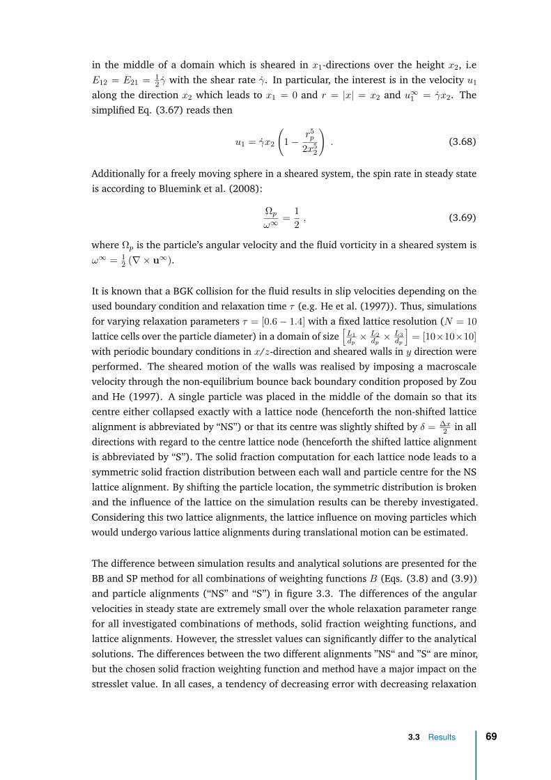
in the middle of a domain which is sheared in x1-directions over the height x2, i.eE12 = E21 = 1

2 γ with the shear rate γ. In particular, the interest is in the velocity u1

along the direction x2 which leads to x1 = 0 and r = |x| = x2 and u∞1 = γx2. Thesimplified Eq. (3.67) reads then

u1 = γx2

(1−

r5p

2x52

). (3.68)

Additionally for a freely moving sphere in a sheared system, the spin rate in steady stateis according to Bluemink et al. (2008):

Ωp

ω∞= 1

2 , (3.69)

where Ωp is the particle’s angular velocity and the fluid vorticity in a sheared system isω∞ = 1

2 (∇× u∞).

It is known that a BGK collision for the fluid results in slip velocities depending on theused boundary condition and relaxation time τ (e.g. He et al. (1997)). Thus, simulationsfor varying relaxation parameters τ = [0.6− 1.4] with a fixed lattice resolution (N = 10lattice cells over the particle diameter) in a domain of size

[L1dp× L2

dp× L3

dp

]= [10×10×10]

with periodic boundary conditions in x/z-direction and sheared walls in y direction wereperformed. The sheared motion of the walls was realised by imposing a macroscalevelocity through the non-equilibrium bounce back boundary condition proposed by Zouand He (1997). A single particle was placed in the middle of the domain so that itscentre either collapsed exactly with a lattice node (henceforth the non-shifted latticealignment is abbreviated by “NS”) or that its centre was slightly shifted by δ = ∆x

2 in alldirections with regard to the centre lattice node (henceforth the shifted lattice alignmentis abbreviated by “S”). The solid fraction computation for each lattice node leads to asymmetric solid fraction distribution between each wall and particle centre for the NSlattice alignment. By shifting the particle location, the symmetric distribution is brokenand the influence of the lattice on the simulation results can be thereby investigated.Considering this two lattice alignments, the lattice influence on moving particles whichwould undergo various lattice alignments during translational motion can be estimated.

The difference between simulation results and analytical solutions are presented for theBB and SP method for all combinations of weighting functions B (Eqs. (3.8) and (3.9))and particle alignments (“NS” and “S”) in figure 3.3. The differences of the angularvelocities in steady state are extremely small over the whole relaxation parameter rangefor all investigated combinations of methods, solid fraction weighting functions, andlattice alignments. However, the stresslet values can significantly differ to the analyticalsolutions. The differences between the two different alignments ”NS“ and ”S“ are minor,but the chosen solid fraction weighting function and method have a major impact on thestresslet value. In all cases, a tendency of decreasing error with decreasing relaxation

3.3 Results 69

0

10

20

30

40

50

60

70

80

90

0.6 0.8 1 1.2 1.4

Erro

r[%

]

Relaxation parameter τ

Ωp,NSSxy,NS

Ωp,SSxy,S

(a)BB method with linear B(x, τ)

0

10

20

30

40

50

60

70

80

90

0.6 0.8 1 1.2 1.4

Erro

r[%

]


Ωp,NSSxy,NS

(b)BB method with non-linear B(x, τ)

0

5

10

15

20

25

30

0.6 0.8 1 1.2 1.4

Erro

r[%

]


Ωp,NSSxy,NS

Ωp,SSxy,S

(c)SP method with linear B(x, τ)

0

5

10

15

20

25

30

35

0.6 0.8 1 1.2 1.4

Erro

r[%

]


Ωp,NSSxy,NS

(d)SP method with non-linear B(x, τ)

Fig. 3.3.: Single sphere stresslet Sxy and angular velocity errors Ωp over τ for a freely movingparticle and different lattice alignments NS and S. Piece-wise linear lines connectingthe symbols are for visual guidance and not interpolation curves.

parameter is observed. For the BB method, however, the discrepancy to the analyticalsolution remains over 40% for the smallest τ value and is even further increased if thesolid fraction weighting function is changed from the linear to the non-linear form.The SP Method shows for the nonlinear weighting function a minimum discrepancyof around 10% and might be even decreased for smaller relaxation parameters thanτ < 0.6. However, combining the SP method with the linear solid fraction weightingfunction results in a minimum error of around or less than five per cent for relaxationparameters choosen between 0.65− 0.8. For relaxtion parameters outside this range, adrastic stresslet error increase is observed.

The solid velocity profile and fluid velocity profiles of the analytical solution as wellas from simulations with an optimal relaxation parameter of τ = 0.7 are depicted infigure 3.4. The insets of figure 3.4 show the velocity profiles from the proximity of theparticle surface, indicated by the horizontal green dashed line, to the upper channel wall.The velocity information from only every fourth lattice node is used for figure 3.4. Thevelocity profiles from the simulations show good agreement to the analytical solutionfor most of the lattice nodes between particle and wall. However, the velocity differencebetween simulations and analytical solution grows for decreasing lattice node distance tothe particle. The SP method shows a slightly better agreement to the analtyical velocityprofile in close particle proximity than the BB method. In contrast, inside of the particle


0.5

0.51

0.52

0.53

0.54

0.55

0.56

0.57

0.58

0.59

0.6

0 0.05 0.1 0.15 0.2

Dim

ensi

onle

ssch

anne

lhei

ghty H

Dimensionless velocity ufluid,xuwall

0.5

0.75

1

0 0.5 1

Analytical solutionFluid velocitySolid velocity

(a)BB method

0.5

0.51

0.52

0.53

0.54

0.55

0.56

0.57

0.58

0.59

0.6

0 0.05 0.1 0.15 0.2

Dim

ensi

onle

ssch

anne

lhei

ghty H

Dimensionless velocity ufluid,xuwall

0.5

0.75

1

0 0.5 1

Analytical solutionFluid velocitySolid velocity

(b)SP method

Fig. 3.4.: Fluid velocity profiles of a free single particle in centre of sheared channel with N = 10lattice nodes over the particle diameter and τ = 0.7. Simulation results are comparedto the analytical solution given by (3.68). The exact location of the particle surface isindicated by the horizontal, green, dashed line. Insets: Fluid velocity profile for thesame simulations shown from particle surface to channel wall where only every fourthlattice node is plotted. Piece-wise linear lines connecting the symbols are for visualguidance and not interpolation curves.

volume, all nodes below the horizontal green dashed line, the BB method seems to fulfillthe no-slip condition slightly better in comparison to the SP method.

0.5

0.51

0.52

0.53

0.54

0.55

0.56

0.57

0 0.005 0.01 0.015 0.02

Dim

ensi

onle

ssch

anne

lhei

ghty H

Dimensionless force Fhyd,xFStokes

0.50.520.540.56

0 0.5 1

y H

εs

τ = 0.7τ = 0.9τ = 1.1

(a)BB method

0.5

0.51

0.52

0.53

0.54

0.55

0.56

0.57

0 0.005 0.01 0.015 0.02

Dim

ensi

onle

ssch

anne

lhei

ghty H


0.50.520.540.56

0 0.5 1

y H

εs

τ = 0.7τ = 0.9τ = 1.1

(b)SP method

Fig. 3.5.: Hydrodynamic force profiles of a free single particle in centre of sheared channel withN = 10 lattice nodes over the particle diameter for a varing relaxation parameter τ .The exact location of the particle surface is indicated by the horizontal, green, dashedline. Insets: Shown is the solid fraction over the dimensionless channel height. Piece-wise linear lines connecting the symbols are for visual guidance and not interpolationcurves.

The implications of the slip velocities can be observed by examining the hydrodynamicforces on the lattice nodes covered by the particle. Therefore, the force distributionsfrom simulations with τ = [0.7 ; 0.9 ; 1.1] are shown in figure 3.5 and the correspondingsolid fraction is depicted in the insets of figure 3.5. Consideration of Eqs. (3.20) and(3.21), the hydrodynamic force is zero if the no-slip condition is pefectly fulfilled, i.e.u = us. It is observed that the no-slip condition is seemingly fulfilled by the BB methodwithin the particle volume where the force is nearly zero for all τ on lattice nodes witha solid fraction of εs = 1.0. However, the SP method cannot apparently guarantee aperfect no-slip condition within the particle volume because the found force profiles are

3.3 Results 71

non-zero and slightly changed for varied τ . On the particle surface, where 0 < εs < 1,the hydrodynamic forces are larger for the SP method in comparison to the BB methodfor all relaxation parameters. Furthermore, it is observed that the forces on the particlesurface increase with decreasing relaxation parameter.

The forces over the different particle parts, volume and surface, can be respectivelyintegrated to obtain two stresslet contributions, a volume stresslet contribution Sxy,V olumewhere the lattice node solid fraction is εs = 1 and a surface stresslet contributionSxy,Surface where the lattice node solid fraction is εs < 1. The two contributions, relatedto the analytical stresslet solution, are presented for both methods and specific relaxationparameters in table 3.2. It is found that the major contribution to the total stressletis on the particle surface. For the BB method, the volume part is neglectable, but thesurface contribution is unsufficent to obtain the correct stresslet value. In comparison,the volume part for the SP method is around 16% and the surface part slightly below 90%of the total stresslet. Considering that the change in the force profiles within the particlevolume for a varying relaxation parameter is only minor, it can be concluded that thestresslet accuracy depends mostly on the hydrodynamic forces on the particle surface.

Sxy,V olumeSxy,analytical

Sxy,SurfaceSxy,analytical

SxySxy,analytical

BB method 1.9755e-7 0.3981 0.3981SP method 0.1673 0.8559 1.0232

Tab. 3.2.: Integrated surface and volume stresslet parts over a freely moving sphere in shearedchannel flow. Non-dimensionalised by the analytical stresslet value. Linear weightingfunction and relaxation parameter τ = 0.7 are used for both methods, BB and SP.

0.5Fxdy(dy ≥ 0) 0.5Fxdy(dy ≤ 0) 0.5Fydx(dx ≥ 0) 0.5Fydx(dx ≤ 0) Sxy

BB method 0.0995 0.0995 0.0995 0.0995 0.398SP method 0.2558 0.2558 0.2558 0.2558 1.0232

Tab. 3.3.: Integrated stresslet quadrants over a freely moving sphere in sheared channel flow.Non-dimensionalised by the analytical stresslet value. Linear weighting function andrelaxation paramater τ = 0.7 are used for both methods, BB and SP.

In addition, the different spatially integrated contributions, 0.5dyFx and 0.5dyFx overparticle volume and surface for different particle quadrants are listed in table 3.3. Eachmethod has equal contributions over the four different particle volumes to the totalstresslet indicating a force-free (steady) state. As also seen from the force profiles andprevious discussion about volume and surface stresslet contributions, the different spatialcontributions of the BB method, which does not give the correct stresslet value, are muchsmaller than the contributions of the SP method which results in the correct stressletvalue.

An influence of the boundary conditions can be excluded as a noteworthy change in thestresslet error for an altered domain size is not observed, cf. table 3.4.


[Lxdp× Ly

dp× Lz

dp

]τ = 0.7 τ = 1.1

[10× 5× 10] 3.64% -[10× 10× 10] 2.31% 18.74%[20× 20× 20] 2.16% 18.85%

Tab. 3.4.: Stresslet error for different domain sizes for the SP method with a linear weightingfunction. Particle is freely rotating in a sheared channel flow.

Additionally, the lattice resolution influence was studied by refining the lattice withregard to the lattice numbers over particle diameter. The results are shown in figure3.6(a) for method BB and SP. For a relaxation parameter of τ = 0.7, the difference tothe analytical solution does not change much for the SP method because the stressletvalue is close to the analytical solution. Surprisingly, the error does not change muchfor the BB method. Hence, the same simulations with a relaxation parameter of τ = 1.1were performed because a larger discrepancy (around 20%) for a lattice resolution ofN = 10 was also found for the SP method. The error for the SP method decreases withan increased lattice resolution as it would be expected. However, also for τ = 1.1, the BBmethod results remain roughly similiar for an increased lattice resolution.

0.1

1

10

100

20 3010

Erro

r[%

]

Lattice resolution N = dp4x

Method BB: τ = 0.7Method BB: τ = 1.1Method SP: τ = 0.7Method SP: τ = 1.1

(a)

1

10

100

1 10 100

Erro

r[%

]

Subgrid resolution

Method BBMethod SP

(b)

Fig. 3.6.: Stresslet error for varied lattice resolutions with a fixed subgrid resolution of NSGR =10 in (a) and varied subgrid resolution for fixed lattice resolution of N = 10 in (b).The domain size is

[Lx

dp× Ly

dp× Lz

dp

]= [10× 10× 10], the particle centre position is not

shifted, and the weighting function for B is linear. Piece-wise linear lines connectingthe symbols are for visual guidance and not interpolation curves.

A too coarse lattice resolution is detrimental to describe accurately the particle shapeand transition from fluid to solid. Similarily, it is important to compute accurately thesolid fraction at each lattice node. In figure 3.6(b), simulation results for the stressletcalculation obtained with a fixed lattice resolution of N = 10, a relaxation parameterτ = 0.7, and varied subgrid resolution for the BB and SP method are depicted. Thedifference to the analytical solution is nearly unchanged and a subgrid resolution ofNSGR = 10 should give a good trade-off between accuracy and computational cost.

3.3 Results 73

The differences in the simulation results between BB and SP method could be possiblyexplained by the findings from the analytical analysis in the previous section. Accordingto the analytical analysis, the fluid viscosity is artificially increased on solid coveredlattice nodes for the BB method. Thereby, an increased fluid flow resistance would beexperienced in particle proximity which would in turn lead to decreased fluid velocities.Decreased fluid velocities are indeed found for the BB method in particle proximity asshown in figure 3.4. Moreover, the hydrodynamic force is essentially computed fromthe velocity difference between particle and fluid according to Eq. (3.20). The obtainedforces are thereby smaller, as seen from Fig. 3.5, and thus smaller inaccurate stressletvalues are obtained. The analytical analysis indicates furthermore that the introducedartificial viscosity depends on the relaxation parameter τ . Hence, a decrease of τ wouldlead to a decrease of the artificial viscosity which would explain the found decreasingstresslet error with decreasing relaxation parameter. Furthermore, the stresslet errorindependence from the lattice resolution could be possibly explained by the introducedartificial viscosity in that it is not caused by a numerical discretisation (scheme), but dueto the peculiar formulation of the forcing term for the BB method. Thus, the stressleterror is roughly constant for varying lattice resolutions. In contrast, if an introducedartificial viscosity were introduced by a numerical discretisation scheme, then the errorwould be expected to decrease with an increasing lattice resolution.

3.3.3 Stresslet and torque for a fixed particle in sheared fluid flow

As mentioned in the introduction, the torque computation has been verified in theliterature for the BB method. This is seemingly contradicting to the above stressletfindings considering that the stresslet is the symmetric part of the first moment of thesurface traction and the torque is the antisymmetric part. The single sphere stresslet Eq.(3.66) depends on fluid viscosity, particle radius and strain rate tensor. Therefore, theabove single sphere case was conducted for a fixed particle to demonstrate the differencein stresslet and torque computation. For such a case, the analytical solution for theparticle torque is known and reads according to Guazzelli and Morris (2012):

Ti = 8πηfr3pω∞i . (3.70)

Similarily to the previous section, a domain size of[L1dp× L2

dp× L3

dp

]= [10× 10× 10] with

periodic boundary conditions in x/z-direction and sheared walls in y direction with asingle particle placed exactly in the middle of the domain were carried out. The latticeresolution was chosen on basis of the lattice resolution study in the previous section tobe N = 10 lattice nodes over the particle diameter and the relaxation parameter wasvaried between τ = [0.6− 1.4].

The simulations results are presented in figure 3.7. As in the previous case, the stressletdiscrepancy to the analytical solution decreases mostly with decreasing relaxation pa-


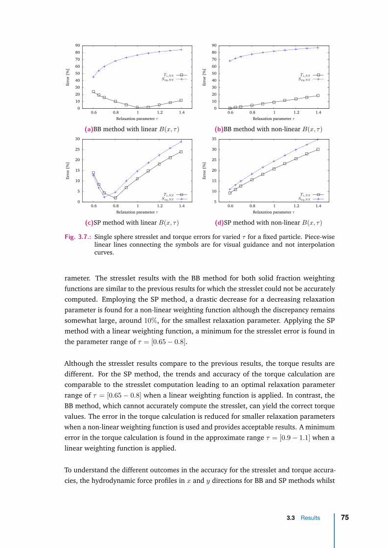
0

10

20

30

40

50

60

70

80

90

0.6 0.8 1 1.2 1.4

Erro

r[%

]


Tz,NSSxy,NS

(a)BB method with linear B(x, τ)

0

10

20

30

40

50

60

70

80

90

0.6 0.8 1 1.2 1.4

Erro

r[%

]


Tz,NSSxy,NS

(b)BB method with non-linear B(x, τ)

0

5

10

15

20

25

30

0.6 0.8 1 1.2 1.4

Erro

r[%

]


Tz,NSSxy,NS

(c)SP method with linear B(x, τ)

5

10

15

20

25

30

35

0.6 0.8 1 1.2 1.4Er

ror

[%]


Tz,NSSxy,NS

(d)SP method with non-linear B(x, τ)

Fig. 3.7.: Single sphere stresslet and torque errors for varied τ for a fixed particle. Piece-wiselinear lines connecting the symbols are for visual guidance and not interpolationcurves.

rameter. The stresslet results with the BB method for both solid fraction weightingfunctions are similar to the previous results for which the stresslet could not be accuratelycomputed. Employing the SP method, a drastic decrease for a decreasing relaxationparameter is found for a non-linear weighting function although the discrepancy remainssomewhat large, around 10%, for the smallest relaxation parameter. Applying the SPmethod with a linear weighting function, a minimum for the stresslet error is found inthe parameter range of τ = [0.65− 0.8].

Although the stresslet results compare to the previous results, the torque results aredifferent. For the SP method, the trends and accuracy of the torque calculation arecomparable to the stresslet computation leading to an optimal relaxation parameterrange of τ = [0.65 − 0.8] when a linear weighting function is applied. In contrast, theBB method, which cannot accurately compute the stresslet, can yield the correct torquevalues. The error in the torque calculation is reduced for smaller relaxation parameterswhen a non-linear weighting function is used and provides acceptable results. A minimumerror in the torque calculation is found in the approximate range τ = [0.9− 1.1] when alinear weighting function is applied.

To understand the different outcomes in the accuracy for the stresslet and torque accura-cies, the hydrodynamic force profiles in x and y directions for BB and SP methods whilst

3.3 Results 75

0.5

0.51

0.52

0.53

0.54

0.55

0.56

0.57

0 0.005 0.01 0.015 0.02 0.025

Dim

ensi

onle

ssch

anne

lhei

ghty H


τ = 1.1

(a)BB method

0.5

0.51

0.52

0.53

0.54

0.55

0.56

0.57

0 0.005 0.01 0.015 0.02 0.025

Dim

ensi

onle

ssch

anne

lhei

ghty H


τ = 0.7

(b)SP method

-0.008

-0.006

-0.004

-0.002

0

0.002

0.004

0.006

0.008

0.44 0.46 0.48 0.5 0.52 0.54 0.56

Dim

ensi

onle

ssfo

rce

Fhyd,y

FStokes

Dimensionless channel length xL

τ = 1.1

(c)BB method

-0.008

-0.006

-0.004

-0.002

0

0.002

0.004

0.006

0.008

0.44 0.46 0.48 0.5 0.52 0.54 0.56

Dim

ensi

onle

ssfo

rce

Fhyd,y

FStokes

Dimensionless channel length xL

τ = 0.7

(d)SP method

Fig. 3.8.: Hydrodynamic force profiles for a fixed particle in centre of a sheared channel withN = 10 lattice nodes over the diameter. The exact location of the particle surfaceis indicated by the green, dashed lines. The force profiles are shown for BB andSP methods combined with a linear solid fraction weighting function along the xand y direction. The relaxation parameter is chosen so that the torque error isminimised. Piece-wise linear lines connecting the symbols are for visual guidance andnot interpolation curves.

applying a linear weighting function with different relaxation parameters are shown infigure 3.8. For both methods, the force profiles in x direction along the y axis, cf. Fig. 3.8(a)/(b), are comparable to the force profiles obtained in simulations of the freely rotatingsphere (Fig. 3.5). However, the surface forces are somewhat larger in the fixed spherecase. For the forces in y direction along the x axis, Fig. 3.8 (c)/(d), the surface forcesfor BB and SP methods are smaller in magnitude than the surface forces in x directionalong the y axis. For the SP method, it is observed that the forces on lattice nodes withinthe particle volume have the same direction as the surface forces on the closest surface.However, the opposite is found for the BB method where the force direction is changedwithin the particle volume.

The main difference between the stresslet and torque calculation can be seen by compari-son of the stresslet and torque formulas. Evaluation of Eq. (3.11) for the z-componentleads to:

Tz =Nnodes∑

(Fydx − Fxdy) . (3.71)


The stresslet Sxy is then according to Eq. (3.15):

Sxy =Nnodes∑ (1

2(Fxdy + Fydx)). (3.72)

Comparison of equations (3.71) and (3.72) shows that the difference is an additionand subtraction between different F

⊗r contributions. Therefore, integrated F

⊗r

contributions over specific parts of the particle volume are listed in table 3.5. For theSP method, all F

⊗r contributions are positive. In contrast, the BB methods results

in positive Fxdy contributions, but negative Fydx contributions. Between the SP andBB method, the Fydx contributions are comparable in magnitude. However, the Fxdycontributions obtained from the SP method are approximately twice as large as fromthe BB method. The stresslet is determined by addition of all contributions accordingto equation (3.72). This leads for the SP method to a total stresslet value which is inagreement with the analytical solution. However, the BB method results in a drasticallyunderestimated total stresslet value because the Fxdy contributions are much smallerthan the corresponding SP method contributions. Additionally, the Fydx contributions arenegative leading to a further reduction of the total stresslet value. The torque calculationis a subtraction of Fxdy contributions from the Fydx contributions according to equation(3.71). For the SP method, the large Fxdy contribution would overestimate the torquewhen considered as only contribution. However, it is subtracted from the smaller Fydxcontributions, which has the same sign, and thereby resulting in an accurate total torquecomputation. An accurate total torque is also obtained with the BB method. Yet, theaccurate torque calculation is not achieved due to a subtraction like for the SP method.The Fydx contributions are negative whereas the Fxdy contributions are positive. Thischange of the sign leads effectively to a summation of the contributions according tothe torque calculation (3.71). Thereby, the total Fxdy torque contribution, which wouldunderestimate the total torque calculation when considered as only contribution, iscompensated by the additional Fydx contributions.

0.5Fxdy(dy ≥ 0) 0.5Fxdy(dy ≤ 0) 0.5Fydx(dx ≥ 0) 0.5Fydx(dx ≤ 0) Sxy Tz

BB method 0.212 0.212 -0.093 -0.093 0.238 -1.22SP method 0.423 0.423 0.102 0.102 1.05 -1.284

Tab. 3.5.: Integrated F⊗

r stresslet parts over parts of a fixed sphere in a sheared channel flow.Non-dimensionalised by the analytical stresslet value. Sxy =

∑0.5(Fxdy + Fydx) and

Tz =∑

(Fydx − Fxdy) where Tanalytical

Sanalytical= 1.2.

3.3 Results 77

3.3.4 Stresslet for two fixed particles in sheared fluid flow

Fig. 3.9.: Simulation setup of two particles placed between two sheared walls to verify thestresslet computation.

Similar to the previous section, the particle stresslet was determined in a sheared systemof the same size, but for two particles as illustrated in figure 3.9. Both particles had thesame size and a lattice resolution of N = 10 lattice nodes over the particle diameter waschosen. The system was sheared so that a Reynolds number of Re = 0.1 was obtained.The analytical solution for a stresslet in a two particle system with particles of radii rp,1and rp,2 was derived by Batchelor and Green (1972b):

S′ij = 20

3 πr3p,1ηf

(Eij(1 +K

′) + Ekl

(rirkδjl + rjrkδil

r2 − rkrlr2

23δij

)L

′

+Eklrkrlr2

(rirjr2 −

13δij

)M

′) (3.73)

where

K′ = −

r3p,2(r2

p,1 + r2p,2)

r5 +O(

(rp,1 + rp,2)6

r6

), (3.74)

L′ = −

5r3p,2

2r3 +5r3p,2(r2

p,1 + r2p,2)

r5 + 25r3p,1r

3p,2

4r6 +O(

(rp,1 + rp,2)6

r6

), (3.75)

M′ = −

25r3p,2

2r3 +35r3

p,2(r2p,1 + r2

p,2)r5 + 25

r3p,1r

3p,2

4r6 +O(

(rp,1 + rp,2)6

r6

), (3.76)


and r is the vector between the particle-particle-centres. With the same conditions andsimplifcations as in the previous section, namely a shearing motion in x1 direction (i.eE12 = E21 = 1

2 γ), the stresslet for i = 1 and j = 2 reads:

S′12 = 20

3 πr3p,1ηf

(12 γ(1 +K

′) + 12 γr1r1 + r2r2

r2 L′ + γ

(r1r2r2

)2M

′). (3.77)

The relaxation parameter was varied between τ = 0.6− 1.4 and the difference betweensimulation results and analytical solution are shown in figure 3.10. The obtained resultsare very similar to the single particle case. For the BB method, the discrepancy decreaseswith decreasing relaxation parameter for all weighting function combinations. Althoughthe discrepancy is larger when using a non-linear weighting function. The BB Methodcannot reproduce the stresslet and shows a minimum discrepancy of more than 40% withthe linear solid fraction weighting function.

In contrast, the SP method can also yield the stresslet in the two particle case correctlywhen a linear function for the solid fraction is considered and the relaxation parameterrange lies between around τ = 0.65 − 0.8. Non-linear weighting of the solid fractionresults similarly to the single sphere case in an increased difference to the analyticalsolution.

0

10

20

30

40

50

60

70

80

90

0.6 0.8 1 1.2 1.4

Erro

r[%

]


BB-NSSP-NS

(a)Linear B(x, τ).

0

10

20

30

40

50

60

70

80

90

0.6 0.8 1 1.2 1.4

Erro

r[%

]


BB-NSSP-NS

(b)Non-linear B(x, τ).

Fig. 3.10.: Stresslet error of two freely rotating particles in shear flow (Re = 0.1) for a variedrelaxation parameter τ with a lattice resolution of N = 10 lattice cells over a particlediameter for methods BB and SP with different weighting functions B. Piece-wiselinear lines connecting the symbols are for visual guidance and not interpolationcurves.

3.3 Results 79

3.3.5 Stresslet contribution in sheared suspensions

Fig. 3.11.: 3D simulation setup of a sheared suspension illustrated on a slice through the domain.The particle distribution is shown on the left and the fluid velocity component inhorizontal direction on the right.

Hitherto, the computation of the stresslet has been analysed on a particle scale. Inthis section, the effect of the stresslet computation for the BB and SP methods on thesuspension viscosity and stress contributions on a bulk scale are investigated. Therefore,simulations in a shear cell under simple shear were performed with an imposed shearrate resulting in a low Reynolds number regime, i.e. Re = d2

pγ

ν < 1. The shear cell wasrealised by imposing a combination of DEM boundary conditions which are conceptuallyequivalent to Lees-Edwards boundary conditions (LEbc), cf. Lees and Edwards (1972),and LEbc for LBM, cf. Wagner and Pagonabarraga (2002), on a three dimensionalperiodic simulation domain The simulation setup with particle distribution and fluidvelocity is exemplarily illustrated on a slice through the simulation domain in figure 3.11.Around 500 neutrally buoyant frictionless mono-disperse particles were suspended ina Newtonian fluid. Different solid fractions were obtained by varying the domain sizeunder the restriction of having a minimum size of at least

[L1dp× L2

dp× L3

dp

]≥ [10×10×10].

Moreover, the lattice resolution was chosen so that N = 10 lattice nodes cover a particlediameter. The focus was on the stresslet contribution to the total stress. Hence, thesolid fraction range was limited to φmax = 0.25 to minimise particle-particle interactionsand thereby avoid lubrication force modelling. In the case of particle collisions, aHooke spring contact model was employed and resulting stress contributions from themechanical contact were computed according to Thompson et al. (2009).

The divergence of the suspension viscosity with increasing solid fraction can be describedby the semi-empirical Krieger-Dougherty correlation, Krieger and Dougherty (1959), i.e.:

ηs =(

1− φ

φmax,mono

)−[η]φmax,mono, (3.78)


where the intrinsic viscosity [η] and maximum packing fraction φmax,mono have to bedetermined by comparison to experiments. According to Debbas and Rumpf (1966) andHaughey and Beveridge (1969), the close random packing for mono-sized spheres is in arange of around 0.615 ≤ φmax,mono ≤ 0.641 which is also in accordance to experimentalinvestigations carried out by Werff and Kruif (1989). Werff and Kruif (1989) determine,besides the maximum packing fraction φmax,mono = 0.63, furthermore the exponent[η]φmax,mono = 2 for the Krieger-Dougherty correlation. The experimental findings ofWerff and Kruif (1989) are adopted for comparison to the simulation results obtainedwith the BB and SP method. An additional Krieger-Dougherty correlation (3.78) with theparameters [η]φmax,mono = 1.8 and φmax,mono = 0.64 was determined by fitting to the SPsimulation results.

1

1.2

1.4

1.6

1.8

2

2.2

2.4

2.6

2.8

3

0 0.05 0.1 0.15 0.2 0.25

Dim

ensi

onle

ssvi

scos

ityη s

=µf

+µp

µf

Solid fraction φ

BB Method

SP Method(1− φ

0.63

)−2(1− φ

0.64

)−1.8

Fig. 3.12.: Apparent viscosity for varied solid fractions of sheared frictionless mono-dispersesuspensions. Piece-wise linear lines connecting the symbols are for visual guidanceand not interpolation curves.

The Krieger-Dougherty correlations and simulation results are shown in figure 3.12. Forboth methods, an increase of the suspension viscosity is found for higher solid fractions.However, the BB method shows a large discrepancy to the Krieger-Dougherty correlations.The SP method, in contrast, captures relatively accurately the viscosity increase. Thedifferences to the findings of Werff and Kruif (1989), which grow with increasing solidfraction, could be explained by a missing lubrication force correction when particles arein close contact.

The different stress contributions to the particle stress ηp for the different solid fractionsare presented for the BB and SP method in figures 3.13(a) and (b), respectively. The stress,non-dimensionalised by the fluid stress ηf γ, is dominated by the stresslet contribution forboth methods. The contact stress contributions are much smaller for low solid fractionsand increase for higher solid fractions due to a growing probability of colliding particles,but remain well below the stresslet values. Although the qualitative trend of the stress

3.3 Results 81

0.001

0.01

0.1

1

10

0.05 0.1 0.15 0.2 0.25

Dim

ensi

onle

ssst

ress

σiηγ

Solid fraction φ

ContactStresslet

(a)BB method

0.001

0.01

0.1

1

10

0.05 0.1 0.15 0.2 0.25

Dim

ensi

onle

ssst

ress

σiηγ

Solid fraction φ

ContactStresslet

(b)SP method

Fig. 3.13.: Dimensionless stress contributions for varying solid fractions for methods BB and SP.

contributions between the BB and SP methods are similar, quantitatively the contributionsbetween both methods differ. Especially, the stresslet contribution for all solid fractionsare larger for the SP method in comparison to the BB method. Thus, the accuracy of thestresslet computation on particle scale, as discussed in the previous sections, affects alsothe stresslet value on bulk scale and ultimately, the stresslet difference leads to the largeviscosity discrepancy found in figure 3.12. Therefore, an accurate stresslet computationis of paramount importance. It is here found that only the SP method leads to realisticvalues on particle and bulk scale.

Furthemore, it shall be remarked that a stress contribution from a lubrication forcecorrection would be expected to fall between the stresslet and contact stress contributions.Thereby, leading to increased suspension viscosities and hence better agreement betweensimulation results and the experimental findings of Werff and Kruif (1989). An inclusionof a lubrication force correction shall however be subject in subsequent chapters as thefocus was here on a correct stresslet computation.

3.4 Conclusions

Two different solid phase collision terms for the immersed moving boundary methodin LBM were evaluated theoretically and numerically with regard to the accuracy tocompute the stresslet. One solid collision term, abbreviated as BB method, was inspiredby the non-equilibrium bounce back. The other solid collision term is abbreviated as SPmethod according to the method’s name (superposition method). Numerical studies wereconducted on particle scale for single and two particles in a sheared domain as well as forbulk suspensions under simple shear. Stresslet simulation results on particle scale werecompared to analytical solutions and the influence of the single relaxation parameter forthe fluid phase collision term on the stresslet accuracy was investigated. Bulk suspensionviscosities were compared to the semi-empirical Krieger-Dougherty correlation and thevarious stress contributions were compared.


The theoretical analysis demonstrates that the partially saturated cell method can bere-written to the common LB notation with an external force. In case of the SP method,the external force can be interpreted as Kuperstokh external force whereas the complexityof the BB method lacks interpretation. The re-written LB equation has been analysed andit has been shown that the SP method leads to additional error terms on macroscale. TheBB method, which is more complex, results in similar additional error terms. However,the BB method affects also moreover the stress tensor by an artificial increase of theviscosity on solid covered lattice nodes. The additional artificial viscosity depends onthe solid fraction of the lattice nodes, single relaxation parameter, density, and speed ofsound.

For the single sphere case, it has been shown that variation of the single relaxation param-eter changes slip velocities between particle and fluid velocities and thus hydrodynamicinteraction forces. Only the SP method achieves an accurate computation of the stressletfor a relaxation parameter in the range of around τ = [0.65−0.8]. The BB method resultsin discrepancies of at least 40% compared to the analytical solution. Similarly, only theSP method leads to accurate stresslet computations for a two particle case in contrast tothe BB method.

Moreover, the correct torque calculation, but failing stresslet calculation, has beenexplained by examining sheared flow around a fixed particle. Analysis of force profilesover the particle for the BB and SP methods revealed flipped force directions along theshearing axis for the BB method in comparison to the SP method. Thereby, leading toincorrect stresslet calculations, but correct torque calculations for the BB method. Incontrast, force profiles over the particle for the SP method are consistent for all directionsand thus lead to accurate torque as well as stresslet computations.

For sheared suspensions consisting of hundreds of particles, large viscosity discrepanciesfor the investigated solid fraction range φ ≤ 0.25 between the BB and SP method arefound. The SP method leads to accurate viscosity values when compared to a Krieger-Dougherty correlation, whereas the BB method significantly underestimates the viscosityvalues. The inaccurate stresslet computation on particle scale, which in turn leads tosmaller bulk stresslet values for the BB method in comparison to the SP method, hashence a direct effect on the resulting viscosity values.

It is advised for future LBDEM simulations with a partially saturated cell method that theSP method is used instead of the BB method.

3.4 Conclusions 83

4Lubrication force calibration of apartially saturated cell method forthe lattice Boltzmann method

4.1 Introduction

A variety of fluid-solid coupling approaches were proposed and commonly used aremethods which solve the fluid flow on a fixed Eulerian lattice and track particles in aLagrangian framework, e.g. Ladd (1994a) and Ladd (1994b), Noble and Torcyznski(1998), or Feng and Michaelides (2005). However, no matter which approach, computa-tional expenses lead to limitations with regard to the fluid flow resolution. A fine latticeresolution to resolve very small gap distances and arising lubrication forces betweenparticles is thus impossible. Yet, lubrication forces are important to consider to describeproperly the microscale suspension physics. A remedy was proposed by Nguyen and Ladd(2002) by introducing lubrication force corrections to model hydrodynamic solid-solidinteractions for unresolved small gap distances.

In this chapter it is shown that the proposed lubrication force correction, which wasdeveloped for the methodology proposed by Ladd (1994a) and Ladd (1994b), can alsobe used to some extent, and after some calibration, in combination with the partiallysaturated cell method suggested by Noble and Torcyznski (1998). Therefore, the appliedmethodology and the lubrication force correction is discussed firstly. Thereafter, closerange hydrodynamic interactions between two particles, subject to the lattice resolution,are simulated. On this basis, recommendations for the single relaxation parameterchoice, which affects the slip velocities and hence forces between fluid and particles,are provided. Furthermore, the applicability of the aforementioned lubrication forcecorrections is investigated with calibration recommendations to minimise discrepanciesbetween simulation results and known analytical solutions.

4.2 Methodology

85


A discrete element method (DEM), e.g. Cundall and Strack (1979), is used to solveNewton’s second law for translational and angular motion with a velocity-Verlet algorithmfor each particle. The total force and torque acting on a particle can be split into particle-particle contacts FC and TC , hydrodynamic interactions FH and TH determined by theLBM and an imposed lubrication force correction FL and TL for short particle-particlegap distances which cannot be resolved by the LBM. The translational motion can beexpressed as:

mi∂x2

i

∂2t= Fi = FC

i + FHi + FL

i . (4.1)

Similarly for the angular motion, it can be written:

Ji∂ωi∂t

= Ti = TCi + TH

i + TLi . (4.2)

Mass, position, moment of inertia and angular velocity of particle i are described by mi,xi, Ji and ωi, respectively.


Fluid dynamics can be described by the Boltzmann equation which is a transport equationfor a particle distribution function. In a particle distribution function f(x,u, t), the fluidmolecules are statistically summarised in a six dimensional space divided in a velocityspace u at position x at time t. Discretisation of the Boltzmann equation leads to thelattice Boltzmann method (LBM). The discretised system consists of a numerical mesh, thelattice, and on each lattice node discrete particle distribution functions fi(x, t) undergoa collision and streaming step. The discrete particle distribution functions fi(x, t) arerelaxed towards an equilibrium distribution function feqi (x,u, t) during the collision stepwhere u is the macroscopic fluid velocity. In the simplest case, the collision occurs viaa single relaxation parameter τ , known as the Bhatnagar-Gross-Krook (BGK) collisionaccording to Bhatnagar et al. (1954):

ΩBGKi = ∆t

τ(feqi (x,u, t)− fi(x, t)) . (4.3)

During the streaming step, each distribution is moved according to pre-defined lattice ve-locities ci to adjacent lattice nodes. Streaming and BGK collision step can be summarisedto the discrete lattice Boltzmann equation:

fi(x + ci∆t, t+ ∆t) = fi(x, t) + ΩBGKi , (4.4)

where the lattice velocities ci are chosen so that macroscale conservation equations formass and momentum (Navier-Stokes equations) are obtained. The relaxation parameter

86 Chapter 4 Lubrication force calibration of a partially saturated cell method

τ is related to the fluid viscosity ν = (τ − 0.5)/3. Details of deriving the macroscopicconservation equations can be found for example in Succi (2001) and Krüger et al.(2017). Macroscopic fluid density and velocity can be obtained by computing thezeroth and first moments of the particle distribution functions, i.e. ρ =

∑i fi(x, t) and

ρu =∑i fi(x, t)ci.

4.2.3 Fluid-solid coupling

Noble and Torcyznski (1998) proposed that the presence of particles can be accountedfor by including an additional collision term Ωs and a weighting function B(x, τ) for thesolid phase so that Eq. 4.4 reads:

fi(x + ci∆t, t+ ∆t) = fi(x, t) +(

1−∑s

B(x, τ))

ΩBGKi +

∑s

B(x, τ)Ωsi . (4.5)

If two particles overlap on one lattice cell, the weighting function B(x, τ) for solidfractions was modified to B1 = B1

B1+B2and B2 = B2

B1+B2for each particle contribution.

As shown in the previous chapter, choice of the solid phase collision term, weightingfunction and relaxation parameter are not straightforward. Thus, the previous chapter’srecommendation was followed and the following solid phase collision term was used:

Ωsi = feqi (us)− fi(x, t) +

(1− ∆t

τ(fi(x, t)− feqi (u)

). (4.6)

A linear relationship to the lattice node solid fraction,

B(x, τ) = εs , (4.7)

was chosen and the single relaxation parameter choice is studied with regard to theresolution of lubrication force between two particles in a later section.

The hydrodynamic force and torque from the fluid phase on the particle can be computedby summing the product between solid phase collision term Ωs

i , solid fraction weightingfunction B, and lattice velocities ci, over all solid covered lattice nodes with a latticespacing of h in d dimensions:

FH = hd

∆t∑n

Bn∑i

Ωsici , (4.8)

TH = hd

∆t∑n

(x− xs)×(Bn∑i

Ωsici

)= hd

∆t∑n

(x− xs)× FH . (4.9)

4.2 Methodology 87

4.2.4 Lubrication force corrections

The fluid flow resolution is limited by the lattice resolution. Considering two approachingparticles, the lubrication forces can be in theory resolved down to a gap distance ofone lattice cell width. For smaller gap distances, Nguyen and Ladd (2002) proposed alubrication force correction on basis of the analytical solution for pairwise lubricationforces between particles. The idea is that the lubrication force is ideally resolved to acertain gap distance between particles, around the size of one lattice cell width. Forsmaller gap distances, the analytical solution is evaluated at two points: At the resolutionlimit and the current gap distance. The difference between both forces is the lubricationforce correction which can be added to the DEM procedure as an additional particle forceas expressed in Eqs. (4.1) and (4.2).

Lubrication forces between particles have been extensively studied and a comprehensiveoverview is provided by Jeffrey and Onishi (1984), Jeffrey (1992) and Kim and Karrila(2005). Arising lubrication interactions between two particles can be expressed in agrand-resistance-matrix notation:

F1

F2

T1

T2

S1

S2

= ηf

A11 A12 B11 B12 G11 G12

A21 A22 B21 B22 G21 G22

B11 B12 C11 C12 H11 H12

B21 B22 C21 C22 H11 H12

G11 G12 H11 H12 M11 M12

G21 G22 H21 H22 M21 M22

v∞(x1)− U1

v∞(x2)− U2

Ω∞ − ω1

Ω∞ − ω2

E∞

E∞

. (4.10)

The subscripts of tensor elements in the resistance matrix, e.g. in general Pαβ, describeforce, torque, and stresslet of particle α while taking into account the motion of particleβ. The focus is here only on the forces and torques. The stresslet and stress computationwas studied in the previous chapter. The lubrication interaction on particle α with aparticle diameter ratio γ to particle β and dimensionless particle-particle gap distanceξ = hgap

rαcan then be generally expressed as:

FLα(γ, ξ) = ηf (Pαα(γ, ξ)Uα + Pαβ(γ, ξ)Uβ) . (4.11)

According to Nguyen and Ladd (2002), consideration of only the leading order terms inthe resistance terms, allow to use only the particle velocities. The correction for smallgap distances reads then:

FLα,correction(γ, ξ) = FL

α(γ, ξ)− FLα(γ, ξN ) , (4.12)

where ξN is the minimal resolvable gap distance, e.g. ξN = hlattice.


4.3 Results

4.3.1 Lubrication force resolution

4.3.1.1. Normal lubrication force

Fig. 4.1.: Simulation set-up to study normal lubrication forces between two particles.

At first, the methodology’s capability to resolve the lubrication force without any correc-tion was studied in a three dimensional periodic system in which the simulation domainlengths Li corresponded to

[Lxdp× Ly

dp× Lz

dp

]= [10× 10× 10]. As illustrated in figure 4.1,

a constant velocity was imposed on two particles of diameter dp so that they approacheach other with a low Reynolds number of Re = dpU

ν = 0.1 along the centre-to-centreline. A lattice resolution of N = 10 lattice cells over the particle diameter dp was chosenand the relaxation parameter τ was varied.

1

10

100

1000

0.01 0.1 1

Dim

ensi

onle

ssno

rmal

forc

efn

fStokes

Number of lattice cells in gap

Analyticalτ = 0.6τ = 0.65τ = 0.7τ = 0.9τ = 1.1τ = 1.3

(a)

0

5

10

15

20

25

30

35

0.5 1 1.5 2 2.5 3 3.5 4 4.5 5

Erro

r[%

]


τ = 0.6τ = 0.65τ = 0.7τ = 0.9τ = 1.1τ = 1.3

(b)

Fig. 4.2.: Dimensionless normal lubrication force (a) and percent difference to the analyticalsolution (b) over the gap distance. Dashed lines represent actual simulation resultswhere the corresponding symbols represent selective data points for visual guidance.

The obtained hydrodynamic forces are non-dimensionalised by the Stokes force FStokes =3πηfrp∆Urelative, where ηf is the dynamic viscosity and rp the particle radius, and aredepicted as a function of the dimensionless gap distance ξ = hgap

rpin figure 4.2a. The

4.3 Results 89

simulation results are compared to the analytical solution derived by Jeffrey (1982)which reads for monodisperse particles in dimensionless form:

fnfStokes

= 12ξ −

920 log(ξ) + 1.3456− 3

56ξlog(ξ) + 0.19ξ . (4.13)

The obtained hydrodynamic forces from the simulations depend on the relaxation pa-rameter τ which is rather unsurprising considering that slip velocities are caused by asingle relaxation parameter scheme as demonstrated by for example He et al. (1997).Larger relaxation parameter values underestimate the lubrication force. A decrease of therelaxation parameter results in an increase of the obtained lubrication force from LBMsimulations to the point that a further decrease leads to an overestimation. The deviationin per cent between analytical solution and simulation results over the gap distance isshown in figure 4.2b. For far distances, discrepancies of over 5% are found for largerrelaxation parameters, τ ≥ 0.9, and a small relaxation parameter τ = 0.6. Furthermore,for these relaxation parameters the error increases for decreasing gap distances. However,intermediate relaxation parameter values, in the narrow range of τ = 0.65− 0.7, leadto acceptable accuracies for larger gap distances with an adequate lubrication forceresolution down to small gap distances. Furthermore, the hydrodynamic force is notinstantly constant when particles start to overlap, but increases to a constant value atgap distances smaller than the theoretical resolvable limit of one lattice cell width.

0

5

10

15

20

25

30

35

40

45

0.6 0.8 1 1.2 1.4

Erro

r[%

]


Averaged ErrorError at ξN = hlattice

(a)

0

5

10

15

20

25

30

35

40

45

50

0.6 0.8 1 1.2 1.4

Erro

r[%

]


Averaged errorError at ξN = hlattice

(b)

Fig. 4.3.: Normal lubrication force errors for particle motion aligned to lattice grid (a) anddiagonal to the lattice (b). Piece-wise linear lines connecting the symbols are for visualguidance and not interpolation curves.

The results were quantified by two measures. Firstly, differences at a gap distance of onelattice cell width, hgap = hlattice, were evaluated. Secondly, an artificial increase in thehydrodynamic force is observed for a small relaxation parameter of τ = 0.6. This lead tocomputation of the averaged discrepancy for gap distances between one and one-halftimes the lattice width, i.e. 1.0hlattice < hgap < 1.5hlattice as an additional measure. Theresults for both accuracy measures for varying relaxation parameters and two differentsimulation set-ups are presented in figure 4.3a and 4.3b. In figure 4.3a, the particleset-up and motion is as illustrated in figure 4.1. Both particles’ motion is aligned to thelattice structure. In the second case, the particles are placed towards the upper right and


lower left corners of the simulation domain so that the normal relative motion occursdiagonally to the lattice grid. In both cases, the two discrepancy measures follow thesame trends and the values differ only slightly. The error decreases from larger relaxationparameter values to a minimum around the relaxation parameter range τ = [0.65− 0.7]and increases then again drastically for smaller values.

4.3.1.2. Lubrication interactions due to relative tangential motion

Fig. 4.4.: Particle location and the magnitude of the fluid velocity field for two particles undergo-ing relative tangential motion.

The lubrication force and torque contribution from relative tangential motion betweenparticles can be similarly probed as the normal lubrication force component. In asimulation domain of the size

[Lxdp× Ly

dp× Lz

dp

]= [10× 10× 10], two particles, whose

centre were offset to the y-axis, were moved with a constant velocity parallel to the y-axisas depicted in figure 4.4 for three different points in time. The imposed velocities werechosen so that a low Reynolds number Re = 0.1 was obtained and the lattice resolutionwas fixed to N = 10 lattice points over a particle diameter. In the previous section,the normal lubrication force could be relatively accurately captured for a relaxationparameter range of τ = [0.65− 0.7]. Thus, the relaxation parameter was henceforth fixedto τ = 0.65.

Three different contributions can be extracted, viz. normal and tangential forces as wellas a torque. The dimensionless lubrication contributions and differences to the knownanalytical solutions in per cent are shown in figures 4.5, 4.6, and 4.7. The result for thenormal lubrication force contribution, presented in Fig. 4.5, is similar to previous results.

4.3 Results 91

Except that a small increase of the error towards a gap distance of one lattice cell widthis found. This is also discussed in the next paragraph.

1

10

100

1000

10000

0.001 0.01 0.1 1

Dim

ensi

onle

ssno

rmal

forc

efn

fStokes


AnalyticalSimulation

(a)

0

5

10

15

20

0 0.5 1 1.5 2 2.5 3 3.5 4 4.5 5

Erro

r[%

]


(b)

Fig. 4.5.: Normal lubrication force for tangentially passing particles.

1

10

0.001 0.01 0.1 1

Dim

ensi

onle

ssta

ngen

tial

forc

eft

fStokes



(a)

0

5

10

15

20

25

30

35

0 0.5 1 1.5 2 2.5 3 3.5 4 4.5 5

Erro

r[%

]


(b)

Fig. 4.6.: Tangential lubrication force for tangentially passing particles.

The dimensionless tangential force component over particle-particle gap distance ispresented in figure 4.6a. The tangential lubrication force found from the simulationshows a qualitative same increase as the analytical solution for a reducing distancebetween the particles. However, for gap distances smaller than the theoretical resolutionlimit of one lattice cell width, it can be observed that the simulation result shows aslightly steeper increase in the hydrodynamic force for a decreasing gap distance to apoint where it assumes a constant value. This is visible as a “bump” in the error plot 4.6band could be explained with a significantly increased overlap between the particles asit is illustrated in the last timestep of figure 4.4. The overlap results in changed flowpatterns because the particle-particle gap is closed due to an increased solid fraction andhence, resulting in an increased hydrodynamic interaction force. Furthermore, larger gapdistances lead seemingly to an increased discrepancy which could be however explainedwith the validity of the analytical solution for only small gap distances. Overall, for thetangential force component in Fig. 4.6, a small overestimation of the force, around 10%,is found.


0.1

1

10

0.001 0.01 0.1 1

Dim

ensi

onle

ssto

rque



(a)

51015202530354045505560

0 0.5 1 1.5 2 2.5 3 3.5 4 4.5 5

Erro

r[%

]


(b)

Fig. 4.7.: Lubrication torque for tangentially passing particles.

A relative tangential motion between particles leads also to a torque contribution, which ispresented in figure 4.7. Figure 4.7a shows the dimensionless torque, obtained by relatingthe simulation result to Tsimulation

2πηf r2pUrelative

, over the gap distance. Although the hydrodynamictorque grows with a decreasing gap distance, it is obvious that the simulation resultdiffers in its magnitude from the analytical solution. The discrepancy, shown in figure4.7b, is a difference of up to 45 per cent. In contrast to the force contributions, the torquesimulation result reveals a large percentage discrepancy to the analytical solution.

4.3.1.3. Rotational lubrication interactions

Hydrodynamic force and torque acting on the particles can not only arise from trans-lational motion, but also due to rotating particles. Therefore, the same simulationswhich were performed to study normal lubrication forces between particles, as describedin section 4.3.1.1 and illustrated in figure 4.1, were conducted. However, in additionto the translational motion along the particle-particle centre line in a domain of size[Lxdp× Ly

dp× Lz

dp

]= [10× 10× 10], a constant angular velocity of the same magnitude

was imposed on each particle. The particles rotated into the same direction and theobtained Reynolds number was as before Re < 1.0. The lattice resolution was chosen sothat N = 10 lattice cells over the particle diameter dp were obtained and the relaxationparameter is chosen according to the results from the normal lubrication force study, i.e.τ = 0.65.

The normal lubrication force, shown in figure 4.8, does not differ to the previous resultsand thus, the focus is set on the force and torque stemming from the particle rotationwhich are presented in figures 4.9 and 4.10, respectively.

The analytical force and force from simulation, non-dimensionalised by 4πr2pηfΩp, over

particle-particle gap distance are shown in Fig. 4.9a. For larger gap distances, theanalytical solution shows a singular force spike indicating that it is only valid for veryshort gap distances. For short gap distances, the analytical and numerical solution

4.3 Results 93

1

10

100

1000

10000

0.001 0.01 0.1 1

Dim

ensi

onle

ssno

rmal

forc

efn

fStokes



(a)

0

5

10

15

20

0 0.5 1 1.5 2 2.5 3 3.5 4 4.5 5

Erro

r[%

]


(b)

Fig. 4.8.: Normal lubrication force for the case of rotating particles approaching each other alongthe centre-to-centre line.

1e-05

0.0001

0.001

0.01

0.1

1

10

0.001 0.01 0.1 1

Dim

ensi

onle

ssta

ngen

tial

forc

eft

fStokes



(a)

0

20

40

60

80

100

0 0.5 1 1.5 2 2.5 3 3.5 4 4.5 5

Erro

r[%

]


(b)

Fig. 4.9.: Lubrication force resulting from the particle rotation of rotating particles approachingeach other along the centre-to-centre line.

show the same tendency in increasing force for decreasing gap distances. However, aquantitative comparison shows a rather large difference in per cent between simulationand analytical solution (cf. Fig. 4.9b). Furthermore, below the theoretical resolutionlimit, i.e. gap distances smaller than one lattice cell width, an increase of the force to aconstant value is found. Thereby, the hydrodynamic force is increasingly overestimatedfor very small gap distances of around [0.05− 1.0] of a lattice cell width. This is visible asa “bump” in the error figure 4.9b and could be explained, as in the previous section forparticles undergoing relative tangential motion, with a significantly increased overlapbetween the particles.

A similar result is found for the torque contribution which is shown in figure 4.10a. Thetorque, which is non-dimensionalised by the factor 8πr3

pηfΩp, shows the same trend fora decreasing short gap distance as the analytical solution. The difference in per cent,depicted in 4.10b, indicates a similar error behaviour, albeit reduced in its quantity,in comparison to the previously discussed lubrication force arising from rotation. Thedifference to the analytical solution decreases for decreasing gap distances and shows anincrease in the hydrodynamic torque to a constant value for gap distances smaller thanone lattice cell width.


0.1

1

10

0.001 0.01 0.1 1

Dim

ensi

onle

ssto

rque



(a)

0

10

20

30

40

50

60

70

0 0.5 1 1.5 2 2.5 3 3.5 4 4.5 5

Erro

r[%

]


(b)

Fig. 4.10.: Lubrication torque resulting from rotating particles approaching each other along thecentre-to-centre line.

4.3.2 Corrections for lubrication interactions

The hydrodynamic lubrication contributions due to relative tangential motion or rotationbetween particles are extremely small compared to the normal lubrication force. De-pending on the gap distance, the difference to the normal lubrication force contributioncan be of several magnitudes. An accurate modelling of the normal lubrication forceseems therefore much more important than the contributions due to relative tangential orrotational motion. Thus, a rough approximation of other contributions than the normallubrication force could be justified.

4.3.2.1. Normal lubrication force correction

Simulations of colliding particles in normal directions as described in section 4.3.1.1 wererepeated. However, the relaxation parameter was fixed to τ = 0.65 and the lubricationforce correction described in section 4.2.4 was applied. The discrepancy to the analyticalsolution over the gap distance is depicted as black solid line, legend entry δcut = 1.0, infigure 4.11. The lubrication force is drastically overestimated due to the further increaseof the hydrodynamic force for gap distances smaller than one lattice cell width. Takingthis effect into account, the lubrication force correction, Eq. (4.12), is slightly modifiedby shifting the outer cut-off distance to smaller gap distances than one lattice cell width,i.e.


α(γ, ξ)− FLα(γ, δcutξN ) , for ξ ≤ δcutξN = δcuthlattice , (4.14)

where δcut is a calibration parameter for the lubrication force correction.

Shifting the outer cut-off marginally by a factor of δcut = 0.85 leads to an initial im-provement, but for further decreasing gap distances an overestimation of the normallubrication forces remains. The overestimation at small gap distances can be diminished

4.3 Results 95

by reducing the outer cut-off to smaller values. In doing so, the lubrication force is thenhowever increasingly underestimated for gap distances close to the cut-off. Therefore, itseems that there exists an optimum for the cut-off in the range δcut = [0.75− 0.8].

0

2

4

6

8

10

12

14

0 0.5 1 1.5 2 2.5

Erro

r[%

]

Number of lattice cells between particles

δcut = 0.70δcut = 0.75δcut = 0.80δcut = 0.85δcut = 1.00

Fig. 4.11.: Normal lubrication force errors with corrections for different outer cut-offs.

0

2

4

6

8

10

0 1 2 3 4 5

Erro

r[%

]

Number of lattice cells between particles

N = 10N = 15N = 20N = 25N = 30

Fig. 4.12.: Normal lubrication force errors with cut-off corrections δcut = 0.75 for different latticeresolutions. Dashed lines represent actual simulation results where the correspondingsymbols represent selective data points for visual guidance.


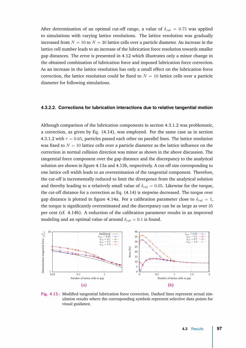
After determination of an optimal cut-off range, a value of δcut = 0.75 was appliedto simulations with varying lattice resolutions. The lattice resolution was graduallyincreased from N = 10 to N = 30 lattice cells over a particle diameter. An increase in thelattice cell number leads to an increase of the lubrication force resolution towards smallergap distances. The error is presented in 4.12 which illustrates only a minor change inthe obtained combination of lubrication force and imposed lubrication force correction.As an increase in the lattice resolution has only a small effect on the lubrication forcecorrection, the lattice resolution could be fixed to N = 10 lattice cells over a particlediameter for following simulations.

4.3.2.2. Corrections for lubrication interactions due to relative tangential motion

Although comparison of the lubrication components in section 4.3.1.2 was problematic,a correction, as given by Eq. (4.14), was employed. For the same case as in section4.3.1.2 with τ = 0.65, particles passed each other on parallel lines. The lattice resolutionwas fixed to N = 10 lattice cells over a particle diameter as the lattice influence on thecorrection in normal collision direction was minor as shown in the above discussion. Thetangential force component over the gap distance and the discrepancy to the analyticalsolution are shown in figure 4.13a and 4.13b, respectively. A cut-off size corresponding toone lattice cell width leads to an overestimation of the tangential component. Therefore,the cut-off is incrementally reduced to limit the divergence from the analytical solutionand thereby leading to a relatively small value of δcut = 0.05. Likewise for the torque,the cut-off distance for a correction as Eq. (4.14) is stepwise decreased. The torque overgap distance is plotted in figure 4.14a. For a calibration parameter close to δcut = 1,the torque is significantly overestimated and the discrepancy can be as large as over 35per cent (cf. 4.14b). A reduction of the calibration parameter results in an improvedmodeling and an optimal value of around δcut = 0.1 is found.

1

10

0.01 0.1 1

Dim

ensi

onle

ssta

ngen

tial

forc

eft

fStokes


Analyticalδcut = 0.05δcut = 0.1δcut = 0.7δcut = 1.0

(a)

0

5

10

15

20

25

30

35

40

0 0.5 1 1.5 2

Erro

r[%

]


δcut = 0.05δcut = 0.1δcut = 0.7δcut = 1.0

(b)

Fig. 4.13.: Modified tangential lubrication force correction. Dashed lines represent actual sim-ulation results where the corresponding symbols represent selective data points forvisual guidance.

4.3 Results 97

0.1

1

10

0.01 0.1 1

Dim

ensi

onle

ssto

rque


Analyticalδcut = 0.05δcut = 0.1δcut = 0.7δcut = 1.0

(a)

0

5

10

15

20

25

30

35

40

45

0 0.5 1 1.5 2

Erro

r[%

]


δcut = 0.05δcut = 0.1δcut = 0.7δcut = 1.0

(b)

Fig. 4.14.: Modified torque due to sheared motion of particles. Dashed lines represent actualsimulation results where the corresponding symbols represent selective data pointsfor visual guidance.

4.3.2.3. Corrections for rotational interactions

The very same simulation setup as described in section 4.3.1.3 with τ = 0.65 andN = 10 lattice cells over a particle diameter was used to calibrate a modified lubricationcorrection Eq. (4.14) for hydrodynamic force and torque arising due to the rotation ofparticles.

0.1

1

10

0.001 0.01 0.1 1

Dim

ensi

onle

ssta

ngen

tial

forc

eft

fStokes


Analyticalδcut = 0.045δcut = 0.5δcut = 1.0

(a)

0

20

40

60

80

100

0 0.5 1 1.5 2

Erro

r[%

]


δcut = 0.045δcut = 0.5δcut = 1.0

(b)

Fig. 4.15.: Modified lubrication force correction for rotational interactions. Dashed lines repre-sent actual simulation results where the corresponding symbols represent selectivedata points for visual guidance.

In figure 4.15a, the force over the gap distance is depicted for a varied calibration cut-off parameter δcut. Similar to the correction for interactions due to relative tangentialmotion, a calibration parameter close to δcut = 1 leads to a huge overestimation of thelubrication force, i.e. nearly 80% in the worst case (cf. Fig. 4.15b). A tremendouslysmaller cut-off has to be choosen to obtain a more accurate lubrication description forsmall gap distances, i.e. δcut ≈ 0.045.

Very similar for a torque correction, depicted in figure 4.16a for torque over gap distanceand in figure 4.16b as difference to the analytical solution in per cent, larger cut-offs


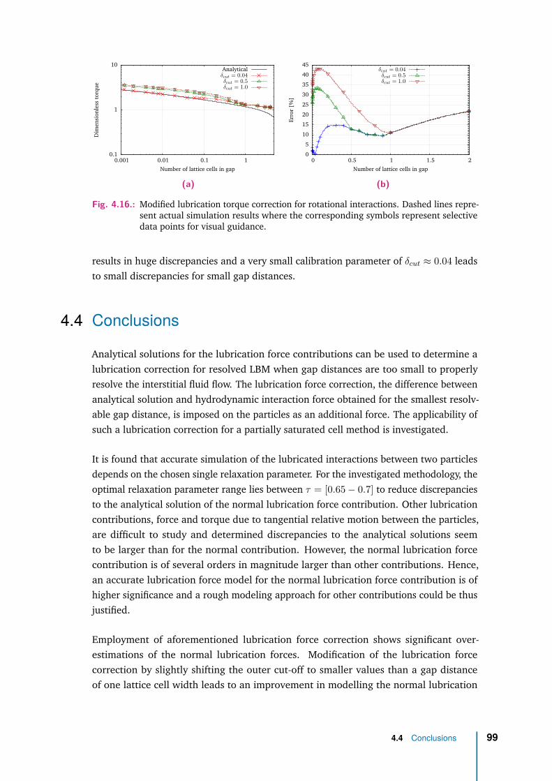
0.1

1

10

0.001 0.01 0.1 1

Dim

ensi

onle

ssto

rque


Analyticalδcut = 0.04δcut = 0.5δcut = 1.0

(a)

0

5

10

15

20

25

30

35

40

45

0 0.5 1 1.5 2

Erro

r[%

]


δcut = 0.04δcut = 0.5δcut = 1.0

(b)

Fig. 4.16.: Modified lubrication torque correction for rotational interactions. Dashed lines repre-sent actual simulation results where the corresponding symbols represent selectivedata points for visual guidance.

results in huge discrepancies and a very small calibration parameter of δcut ≈ 0.04 leadsto small discrepancies for small gap distances.

4.4 Conclusions

Analytical solutions for the lubrication force contributions can be used to determine alubrication correction for resolved LBM when gap distances are too small to properlyresolve the interstitial fluid flow. The lubrication force correction, the difference betweenanalytical solution and hydrodynamic interaction force obtained for the smallest resolv-able gap distance, is imposed on the particles as an additional force. The applicability ofsuch a lubrication correction for a partially saturated cell method is investigated.

It is found that accurate simulation of the lubricated interactions between two particlesdepends on the chosen single relaxation parameter. For the investigated methodology, theoptimal relaxation parameter range lies between τ = [0.65− 0.7] to reduce discrepanciesto the analytical solution of the normal lubrication force contribution. Other lubricationcontributions, force and torque due to tangential relative motion between the particles,are difficult to study and determined discrepancies to the analytical solutions seemto be larger than for the normal contribution. However, the normal lubrication forcecontribution is of several orders in magnitude larger than other contributions. Hence,an accurate lubrication force model for the normal lubrication force contribution is ofhigher significance and a rough modeling approach for other contributions could be thusjustified.

Employment of aforementioned lubrication force correction shows significant over-estimations of the normal lubrication forces. Modification of the lubrication forcecorrection by slightly shifting the outer cut-off to smaller values than a gap distanceof one lattice cell width leads to an improvement in modelling the normal lubrication

4.4 Conclusions 99

force. However, careful calibration of the shifted cut-off distance is required. Similarly,the lubrication correction for the lubrication force and torque due tangential relativeor rotational motion of the particles can be modified to obtain an improved lubricationforce model.


5A comparison study between DEMand LBDEM for simulation of densesuspensions

5.1 Introduction

Kulkarni and Morris (2008) and Haddadi and Morris (2014) performed simulations ofsuspensions under simple shear with a coupled LBDEM approach, proposed by Ladd(1994a) and Ladd (1994b), to study inertial effects on the suspension rheology andmicrostructure. The suspensions of low solid fractions, φ ≤ 0.35, were sheared forvarying Reynolds numbers between 0.005 ≤ Re ≤ 5. Kulkarni and Morris (2008) andHaddadi and Morris (2014) show that with increasing Reynolds number, i.e. increasinginertia, the microstructure, characterised by a pair distribution function, changes althoughthe effect of inertia is diminished for higher solid fractions. Furthermore, it is shown byHaddadi and Morris (2014) that for low Reynolds number flows the stresslet contributionis the largest bulk stress contribution whereas the other contributions, Reynolds andacceleration stresses, become important for Reynolds number of O(Re ≥ 1).

However, simulations employing a LBDEM coupling to simulate suspensions are expen-sive. Hence, some studies applied therefore only a DEM solver with additional models toimitate hydrodynamic and lubrication interactions without any coupling to a fluid resolv-ing solver, e.g Andreotti et al. (2012), Ness and Sun (2015) and Trulsson et al. (2017).Although LBDEM simulations by Kulkarni and Morris (2008) and Haddadi and Morris(2014) indicate that inertia, and hence avoidance of a coupling, could be avoided forlow Reynolds number flows, especially for high solid fractions, only Gallier et al. (2018)compared very recently DEM simulations to simulations employing a fictitious domainmethod (FDM) to solve for Stokes equations describing the fluid flow around suspendedparticles. Gallier et al. (2018) found that obtained suspension viscosities between bothmodelling approaches are effectively the same. However, it is moreover shown that theunderlying microstructures between DEM and FDM differs for pair correlation functions,velocity correlations, and diffusion coefficients for lower solid fractions. Yet, for highersolid fractions, found microstructures are very similar.

In this chapter, intermediate to dense suspensions in a low Reynolds number regime aresimulated with the LBDEM coupling, extensively discussed in the previous chapter, and

101

with DEM employing additional models for hydrodynamic fluid-solid drag and lubricationinteractions. At first, two lubrication model formulations are compared with regard toobtained viscosities and stress contributions. Thereafter, results obtained with one ofthe lubrication force modelling approaches are compared to LBDEM simulation results.Comparison between DEM and LBDEM is performed for viscosities, stress contributions,normal stress differences, and velocity profiles.

5.2 Methodology


By employing a discrete element method (DEM), e.g. Cundall and Strack (1979), themotion of a particle is determined by solving Newton’s second law. A velocity-Verletalgorithm is used to determine the translational and angular velocities as well as thelocation of a particle. Various particle-particle interactions can be considered in the totalforce acting on the particle. Thereby, the equation describing the translational motionreads here:

mi∂x2

i

∂2t= Fi = FC

i + FHi + FL

i . (5.1)

Similarly for the angular motion:

Ji∂ωi∂t

= Ti = TCi + TH

i + TLi , (5.2)

where mass, position, moment of inertia and angular velocity of particle i are describedby mi, xi, Ji and ωi, respectively. The included forces F and torques T on a particleconsist of a mechanical contact when particles overlap (FC and TC), a lubricationinteraction when particles are in close proximity to each other resulting in a mutualinfluence through the surrounding fluid (FL and TL), and a hydrodynamic interactionbetween particle and fluid (FH and TH).

5.2.1.1. Mechanical contact

The basic mechanical contact between particles is modelled through a spring-dashpotmodel in normal as well as tangential contact direction. A multitude of models, such as aHooke or Hertz model, exist to describe the particle-particle contact, e.g. Luding (1998)and Herrmann and Luding (1998). A Hooke model is chosen which leads in normalcontact direction between particles with the relative velocity u to the force

FCn = knδn + γnurel,n (5.3)

102 Chapter 5 A comparison study between DEM and LBDEM for simulation of dense suspensions

and in tangential direction with a history dependent tangential overlap δt to

FCt = ktδt + γturel,t . (5.4)

The spring stiffness in normal and tangential direction is kn and kt, respectively. Thedamping coefficient in normal direction is expressed as γn and in tangential direction asγt. The damping coefficients are chosen to be γn = γt = 0 due to the already existingdissipation caused by lubrication interactions between particles. The tangential springstiffness is chosen in dependence of the normal spring stiffness, kt = 2

7kn, according toSchäfer et al. (1996).

Additional to the elastic-dissipative mechanical contact, friction between particles can beconsidered on basis of a Coulomb friction criterion. A variety of Coulomb-based frictioncriteria exist, e.g. Cundall and Strack (1979), Herrmann and Luding (1998) and Schäferet al. (1996). Each of the suggestions link friction, normal and tangential force via aCoulomb criteria differently. However, for a contact without a dashpot model, as it ishere by setting the damping coefficients to zero, the different friction models lead to thesame criterion which reads then:

|FCt | ≤ |µrFC

n | , (5.5)

where the force tangential to the particle-particle contact, is limited by the product ofcoefficient of friction µr and absolute contact normal force.

5.2.1.2. Hydrodynamic interactions in DEM

Particles immersed in a fluid can have a mutual influence on their motion throughhydrodynamic forces due to relative velocities between the particles itself and betweemthe particles and fluid. A vast amount of work has been carried out to understand anddescribe lubrication interactions between particles, e.g. Jeffrey and Onishi (1984), Jeffrey(1992) and Kim and Karrila (2005).

Instead of considering all possible lubrication interactions for all particles, as it is per-formed for Stokesian dynamics, lubrication effects are introduced as a pure two-particle-particle interaction when the gap distances between both interacting particles falls belowa predefined threshold, henceforth described as outer cut-off δc,o. Therefore, the lubri-cation interaction between two particles can be expressed in a grand-resistance-matrix

5.2 Methodology 103

(GRM) notation, e.g. Jeffrey and Onishi (1984), Jeffrey (1992) and Kim and Karrila(2005), as:

F1

F2

T1

T2

S1

S2

= ηf

A11 A12 B11 B12 G11 G12

A21 A22 B21 B22 G21 G22

B11 B12 C11 C12 H11 H12

B21 B22 C21 C22 H11 H12

G11 G12 H11 H12 M11 M12

G21 G22 H21 H22 M21 M22

v∞(x1)− up,1v∞(x2)− up,2ω∞ − ωp,1ω∞ − ωp,2

E∞

E∞

. (5.6)

The tensor elements in the resistance matrix determine the force on one particle independence of itself and the other particle. Hence, the tensor notation of the resistanceelements, such as A11 or A12, have to be understood that the first subscript gives theparticle on which force, torque, or stresslet act in dependence of the particle stated by thesecond subscript. Here only force and torque on two interacting particles are evaluatedwith the GRM. Instead of determining the separate stresslet values S1 and S2 via lengthyGRM computations to evaluate the particle stress, the particle stress can be determinedfrom the forces itself as is discussed in the subsequent section 5.2.1.3.Computation of the lubrication interactions with the GRM and resistance matrices pro-vided by Kim and Karrila (2005) lead to force and torque contributions arising fromtranslational and angular relative velocities between particles and fluid as well as acontribution from the strain rate tensor. The details of the GRM evaluation and the finalexpressions for force and torque, which were implemented into LIGGGHTS, can be foundin the appendix B. However, the GRM can be also re-written by substituting all relevantresistance matrices and simplifying lengthy expressions under the assumption that forclose gap distances between particles the fluid velocities on the closest particle surfacesare approximately the same. Thereby, the GRM reduces to lubrication expressions basedonly on the relative velocity between two interacting particles and without backgroundfluid velocity components or explicit strain rate contributions. Fluid or strain componentsare indirectly considered within the simplified expressions for forces due to normalcollision, relative tangential and angular velocities as well as torques due to relativetangential and angular velocities. The simplifications were deduced by my colleagueRangarajan Radhakrishnan and implemented into LAMMPS. Both, deductions and codewere made publicly available by Radhakrishnan (2018). I implemented the above GRMmodel (5.6) into LIGGGHTS. My contributions with regard to the simplified GRM workwas limited to LAMMPS coding support, code verification support, and conversion of theLAMMPS code files for use with LIGGGHTS. The simplified expressions read for the forceon a particle:

F = ηf

[X11A up,rel,n + Y 11

A (up,rel,t − (rp,1 + rp,2)(ωs × e))

+1− γ(1 + 4γ)4 + γ

Y 11B (ωd × e)

], (5.7)


where ωs = (ωp,1 +ωp,2)/2, wd = (ωp,1−ωp,2)/2, and up,rel,n and up,rel,t are the normaland tangential component of the relative velocity up,rel = up,2 − up,1 between particles1 and 2. γ describes the particle size ratio between particles 1 and 2. In Eq. (5.7), thefirst term describes lubrication forces in normal collision direction, the second term isdue to relative tangential shearing motion of two particles and the last term representthe lubricated interactions due to particle rotation. The simplified lubrication torqueexpression can be written as:

T = ηf

[Y 11B (up,rel × e) + (rp,1 + rp,2)(ωs − (ωs · e)e)

+Y 12C

(1− 4

γ

)(ωd − (ωd · e)e)

], (5.8)

where the first term arises due to shearing motion between particle surfaces and thesecond term stems from particle rotations. The resistance functions X11

A , Y 11A , Y 11

B , andY 12C are taken to the order of log(ξ−1) with ξ = hgap

rpfrom Kim and Karrila (2005).

In both cases, GRM and simplified GRM lubrication computation, only hydrodynamicinteractions between particles are considered. A simple model to incorporate additionallya drag force from the relative fluid and particle motion can be based on the Stokes singlesphere drag law so that it can be written for the hydrodynamic force

FStokes = 6πηfrp(u∞f (xp)− up) (5.9)

and moreover for the hydrodynamic torque

TStokes = 8πηfrp(ω∞f (xp)− ωp) . (5.10)

The fluid rotation is ω∞f (xp) = 12

(∇× u∞f (xp)

)and for a sheared system, a linear

velocity profile for the fluid velocity can be assumed, i.e. the only non-zero componentsfor the strain rate tensor are Exy = Eyx = 1

2 γ.

5.2.1.3. Stress evaluation

The total bulk stress is decomposed into different contributions: Mechanical particle-particle contact stress σC and contributions based on the lubrication force σL. Forinterparticle forces, such as contact forces or lubrication forces, the stress computationcan be performed for rigid particles according to Thompson et al. (2009) as:

σC = 1V

∑i

∑j

rijFCij (5.11)

5.2 Methodology 105

andσL = 1

V

∑i

∑j

rijFLij , (5.12)

where r is the connecting vector between the interacting particles while pointing fromparticle j to i. A single sphere Stokes drag force, as discussed in the previous section,should be also considered in the stress evaluation for which the stresslet could beexpressed according to the single sphere stresslet (e.g. Guazzelli and Morris (2012)):

Sij = −203 πηfr

3pE∞ij . (5.13)


As discussed above, a single sphere Stokes drag force can be imposed in pure DEMsimulations employing a pairwise lubrication model. However, it is not entirely clear howthis modelling approach affects sheared simulations of dense suspensions and how it isjustified. Therefore, the goal is to resolve the fluid flow around the particles by means ofa lattice Boltzmann method (LBM) which is coupled to DEM for comparison.

In the LBM, fluid molecules are statistically described by a particle distribution functionf(x,u, t) which gives the fluid molecules with velocity u at the location x at time t. Thespatial and temporal evolution of the distribution function is described by the Boltzmannequation and a discretisation with regard to velocities, space and time leads to the latticeBoltzmann method. The discrete distribution function fi(x, t)) is subject to a collision onthe lattice nodes, i.e. relaxation towards a local equilibrium function feqi (x,u, t), and astreaming step at which the distribution functions are moved along pre-defined pathswith the velocities ci towards neighbouring lattice nodes.

The simplest collision step, Bhatnagar-Gross-Krook (BGK) collision after Bhatnagar et al.(1954), relaxes the distribution function towards an equilibrium distribution function feqiover a single relaxation parameter τ :

ΩBGKi = ∆t

τ(feqi (x,u, t)− fi(x, t)) . (5.14)

Combination of the streaming and BGK collision step leads to the lattice Boltzmannequation:

fi(x + ci∆t, t+ ∆t) = fi(x, t) + ΩBGKi . (5.15)

Taking the zeroth and first moments of the distribution functions yields macroscopicfluid density ρ =

∑i fi(x, t) and fluid momentum ρu =

∑i fi(x, t)ci. The macroscale

conservation equations, inter alia the Navier-Stokes equations, can be obtained from thelattice Boltzmann equation (5.15). The detailed derivation can be found elsewhere, e.g.


Succi (2001) and Krüger et al. (2017), and it shall be here only noted that the relaxationparameter τ is linked in this process to the fluid viscosity by ν = (τ − 0.5)/3.

5.2.2.1. Fluid-solid coupling

The hydrodynamic interaction between fluid and particles can be achieved by variousmethods. Here, a fluid-solid coupling proposed by Noble and Torcyznski (1998), whichis analysed in the previous chapters 3 and 4, is used.

In essence, an additional collision term Ωs is introduced to consider interactions betweenparticle distribution functions and a particle on a lattice node. The fluid and solid phaseare differentiated by a weighting function for the solid phase which leads to the modifiedLBM equation:

fi(x + ci∆t, t+ ∆t) = fi(x, t) +(

1−∑s

B(x, τ))

ΩBGKi +

∑s

B(x, τ)Ωsi . (5.16)

The solid collision term reads:

Ωsi = feqi (us)− fi +

(1− ∆t

τ(fi − feqi (u)

). (5.17)

For the weighting function, a linear relationship to the lattice node solid fraction εs,describing the overlap between particle and lattice node, is chosen:

B(x, τ) = εs . (5.18)

The hydrodynamic force and torque on a particle can be obtained by summation of thesolid phase collision term multiplied by the lattice velocities over all lattice nodes coveredby a particle, i.e.:

FH = hd

∆t∑n

Bn∑i

Ωsici , (5.19)

and

TH = hd

∆t∑n

(x− xs)×(Bn∑i

Ωsici

)= hd

∆t∑n

(x− xs)× FH , (5.20)

where h is the lattice spacing in d dimensions.

5.2.2.2. Lubrication correction

The LBM has a limited fluid flow resolution due to the lattice size which means thatlubrication forces between particles can be only resolved to particle-particle gap distances

5.2 Methodology 107

of around one lattice cell width. For smaller gap distances a lubrication force correctionis necessary to model the hydrodynamic particle-particle interactions. Therefore thelubrication force correction discussed in the previous chapter in employed. The correctionis limited to normal lubrication forces and neglects other contributions due to their smalloverall contribution in comparison to normal lubrication forces as shown in the previouschapter 4. The normal lubrication force correction from previous chapter, which is addedto equation (5.1), reads:


α(γ, ξ)− FLα(γ, δcutξN ) , for ξ ≤ δcutξN = δcuthlattice , (5.21)

where γ is the particle size ratio, ξ = hgaprp

the dimensionless gap distance and δcut = 0.75is a cut-off calibration parameter for the lubrication force correction based on the findingsin the previous chapter.

5.2.2.3. Stresslet calculation

As shown in chapter 3, the stresslet in LBM can be computed from the hydrodynamiclattice forces FLBM (cf. eq (5.19)) by summing over all particle covered lattice nodesand particles:

σij,stresslet = − 1V

∑∫Ap

12 (σikxj + σjkxi)nkdA

= − 1V

Nparticles∑ Nnodes∑ (12(FLBMik xj + FLBMjk xi)

),

(5.22)

where the vector xi points from particle centre to the lattice node on which FLBM acts.The negative sign is chosen to make the stresslet computation consistent to the stressesstemming from particle-particle interactions as in Eqs. (5.11) and (5.12).

5.3 Results

A comparison study between the aformentioned LBDEM coupling and different DEMmodels to simulate dense suspensions under simple shear was carried out. Lees-Edwardsboundary conditions (LEbc) for LBM, cf. Wagner and Pagonabarraga (2002), and forDEM conceptually equivalent boundary conditions to LEbc, cf. Lees and Edwards (1972),were imposed on a three dimensional periodic domain as it is depicted on a slice on thex-y-plane through the simulation domain in figure 5.1. The fluid velocity componentin sheared direction uf,x is depicted in the right illustration in figure 5.1 with thecorresponding particle distribution in the left illustration. The particle distribution wasbi-disperse with a diameter ratio of dp,2dp,1

= 1.4, which is commonly used in the literature to

avoid crystallisation, and a volume ratio of Vp,2,totVp,1,tot= 1. In comparison to a mono-disperse


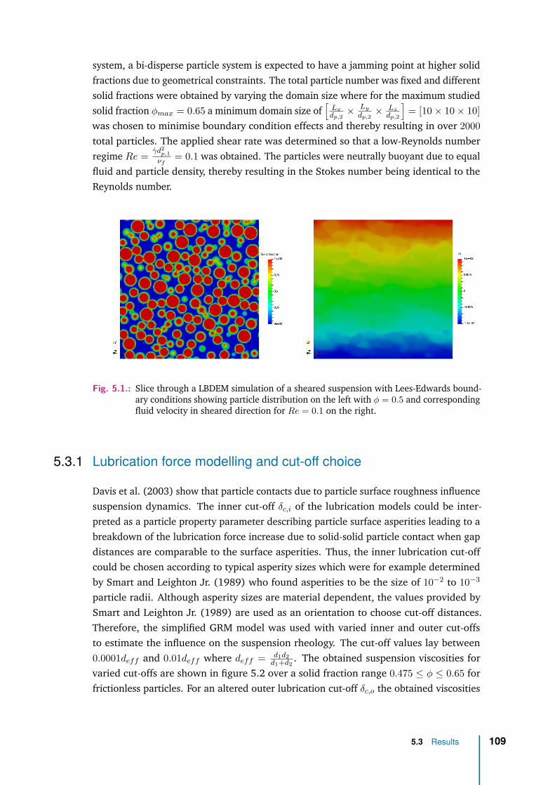
system, a bi-disperse particle system is expected to have a jamming point at higher solidfractions due to geometrical constraints. The total particle number was fixed and differentsolid fractions were obtained by varying the domain size where for the maximum studiedsolid fraction φmax = 0.65 a minimum domain size of

[Lxdp,2× Ly

dp,2× Lz

dp,2

]= [10× 10× 10]

was chosen to minimise boundary condition effects and thereby resulting in over 2000total particles. The applied shear rate was determined so that a low-Reynolds numberregime Re = γd2

p,1νf

= 0.1 was obtained. The particles were neutrally buoyant due to equalfluid and particle density, thereby resulting in the Stokes number being identical to theReynolds number.

Fig. 5.1.: Slice through a LBDEM simulation of a sheared suspension with Lees-Edwards bound-ary conditions showing particle distribution on the left with φ = 0.5 and correspondingfluid velocity in sheared direction for Re = 0.1 on the right.

5.3.1 Lubrication force modelling and cut-off choice

Davis et al. (2003) show that particle contacts due to particle surface roughness influencesuspension dynamics. The inner cut-off δc,i of the lubrication models could be inter-preted as a particle property parameter describing particle surface asperities leading to abreakdown of the lubrication force increase due to solid-solid particle contact when gapdistances are comparable to the surface asperities. Thus, the inner lubrication cut-offcould be chosen according to typical asperity sizes which were for example determinedby Smart and Leighton Jr. (1989) who found asperities to be the size of 10−2 to 10−3

particle radii. Although asperity sizes are material dependent, the values provided bySmart and Leighton Jr. (1989) are used as an orientation to choose cut-off distances.Therefore, the simplified GRM model was used with varied inner and outer cut-offsto estimate the influence on the suspension rheology. The cut-off values lay between0.0001deff and 0.01deff where deff = d1d2

d1+d2. The obtained suspension viscosities for

varied cut-offs are shown in figure 5.2 over a solid fraction range 0.475 ≤ φ ≤ 0.65 forfrictionless particles. For an altered outer lubrication cut-off δc,o the obtained viscosities

5.3 Results 109

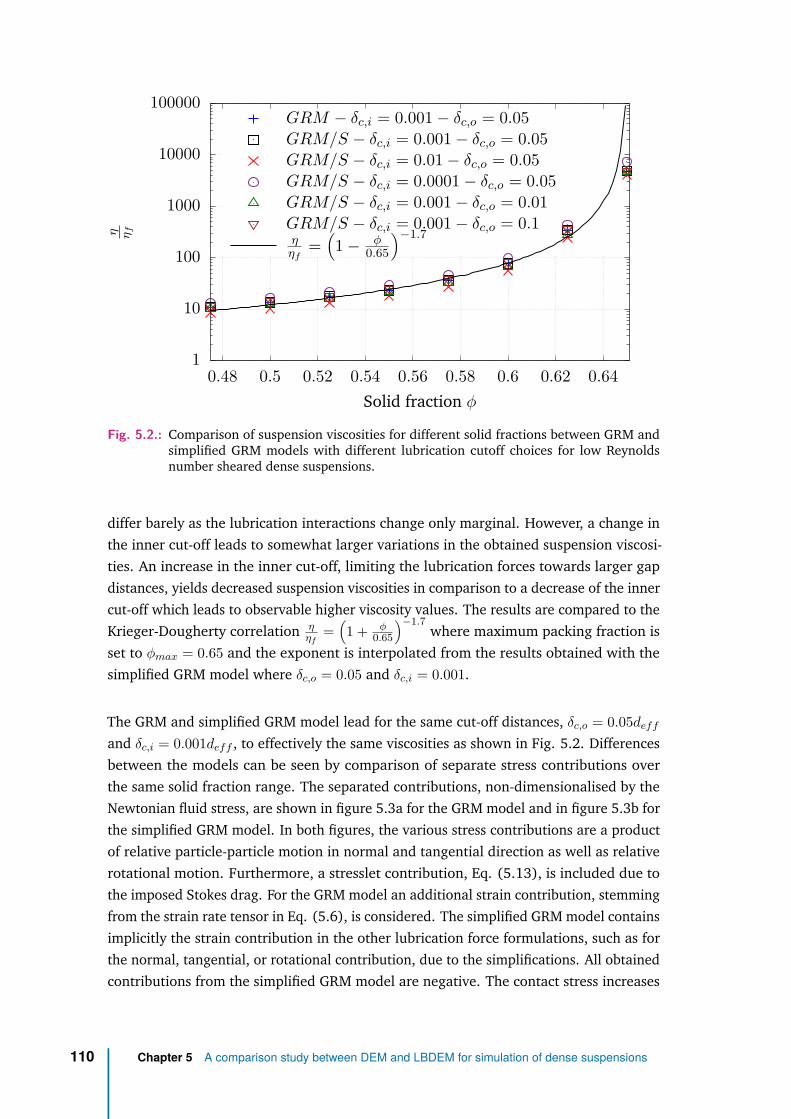
1

10

100

1000

10000

100000

0.48 0.5 0.52 0.54 0.56 0.58 0.6 0.62 0.64

η ηf

Solid fraction φ

GRM − δc,i = 0.001− δc,o = 0.05GRM/S − δc,i = 0.001− δc,o = 0.05GRM/S − δc,i = 0.01− δc,o = 0.05GRM/S − δc,i = 0.0001− δc,o = 0.05GRM/S − δc,i = 0.001− δc,o = 0.01GRM/S − δc,i = 0.001− δc,o = 0.1ηηf

=(1− φ

0.65

)−1.7

Fig. 5.2.: Comparison of suspension viscosities for different solid fractions between GRM andsimplified GRM models with different lubrication cutoff choices for low Reynoldsnumber sheared dense suspensions.

differ barely as the lubrication interactions change only marginal. However, a change inthe inner cut-off leads to somewhat larger variations in the obtained suspension viscosi-ties. An increase in the inner cut-off, limiting the lubrication forces towards larger gapdistances, yields decreased suspension viscosities in comparison to a decrease of the innercut-off which leads to observable higher viscosity values. The results are compared to theKrieger-Dougherty correlation η

ηf=(1 + φ

0.65

)−1.7where maximum packing fraction is

set to φmax = 0.65 and the exponent is interpolated from the results obtained with thesimplified GRM model where δc,o = 0.05 and δc,i = 0.001.

The GRM and simplified GRM model lead for the same cut-off distances, δc,o = 0.05deffand δc,i = 0.001deff , to effectively the same viscosities as shown in Fig. 5.2. Differencesbetween the models can be seen by comparison of separate stress contributions overthe same solid fraction range. The separated contributions, non-dimensionalised by theNewtonian fluid stress, are shown in figure 5.3a for the GRM model and in figure 5.3b forthe simplified GRM model. In both figures, the various stress contributions are a productof relative particle-particle motion in normal and tangential direction as well as relativerotational motion. Furthermore, a stresslet contribution, Eq. (5.13), is included due tothe imposed Stokes drag. For the GRM model an additional strain contribution, stemmingfrom the strain rate tensor in Eq. (5.6), is considered. The simplified GRM model containsimplicitly the strain contribution in the other lubrication force formulations, such as forthe normal, tangential, or rotational contribution, due to the simplifications. All obtainedcontributions from the simplified GRM model are negative. The contact stress increases


0.01

0.1

1

10

100

1000

10000

100000

1e+ 06

0.48 0.5 0.52 0.54 0.56 0.58 0.6 0.62 0.64 0.66

Dim

ensi

onle

ssst

ress−σiηγ

Solid fraction φ

Contact(−1)×Normal lubrication forceTang. lub. force(−1)×Rot. lub. forceStrainStresslet

(a)GRM

0.01

0.1

1

10

100

1000

10000

100000

1e+ 06

0.48 0.5 0.52 0.54 0.56 0.58 0.6 0.62 0.64 0.66

Dim

ensi

onle

ssst

ress−σiηγ

Solid fraction φ

ContactNormal lubrication forceTang. lub. forceRot. lub. forceStresslet

(b)GRM/S

Fig. 5.3.: Stress contributions obtained from the GRM, (a), and simplified GRM models, (b),from corresponding simulations in Fig. 5.2.

and turns into the dominating contribution with increasing solid fraction whereas thenormal and tangential lubrication contributions, which are comparable to each otherin magnitude for all solid fractions, increase only slightly. The stresslet contribution issimilar in its magnitude to the normal and tangential contribution for lower solid fractionvalues, but is nearly unchanged for varying solid fractions. The rotational lubricationstress contribution is much smaller than all other contributions for the whole investigatedsolid fraction range.

In comparison to the simplified GRM model, contributions from the GRM model aredifferent in two aspects for all solid fractions - namely the changed sign of the stressesfor the normal as well as the rotational lubrication component, indicated by the multipli-cation with (−1) in the legend, and futhermore, the huge difference in the magnitude ofthe normal lubrication stress contribution between GRM and simplified GRM.

The opposite sign of the normal lubrication stress contributions between the GRM andsimplified GRM model could be explained by the different reference points in both models.Therefore, a closer look at the contact stress contribution is helpful because the contactforces in the simulations here are always repulsive due to pure repulsive elastic force. Asabove mentioned, the contact stress is here for a positive shear direction and steady-statealways negative. By definition of the stress in Eq. (5.11), the particle-particle connectingvector r points towards the centre of the currently considered particle for which the stressis computed. Thus, the product of rxFCy giving the shear stress σCxy is always negative.Yet, lubrication forces depend also on the particle and fluid velocities in contrast to thecontact model which depends only on the stiffness and particle overlaps. Comparison ofthe lubrication force models, Eqs. (5.6) and (5.7), shows that the difference between thelubrication models is mostly in the considered velocities. In the simplified GRM model,only the relative particle-particle velocities are considered, i.e. up,rel = up,2−up,1. For theGRM model however, the fluid velocity is also part of the force fomula, i.e. v∞(x1)−up,1and v∞(x2) − up,2. This leads to two different reference points. The reference framefor the simplified GRM model is locally with the particles whereas the global system

5.3 Results 111

is the reference frame in the GRM model. Hence, the normal lubrication force of thesimplified GRM model corresponds basically to the sum of the normal lubrication forceand a strain rate force of the GRM model. In fact, in the derivation of the simplifiedexpressions of the lubrication interactions, Radhakrishnan (2018) combined the strainrate contributions with all other contributions to obtain the final equations in (5.7) and(5.8). With regard to the obtained shear stress contributions from simulations employingthe GRM model, the stress magnitude of the strain contribution is slightly larger thanthe normal lubrication force contribution of the GRM model. It could be shown that thesummation of both contributions obtained from the simulations leads to very similar(negative) values obtained by the simplified GRM model for the normal lubrication stresscontribution.

The huge magnitude of the normal lubrication contribution and strain rate contributionobtained with the GRM model could be also understood by the aforementioned explana-tion. As mentioned above, for the simplified GRM model the normal lubrication forcecorresponds to the sum of the normal lubrication force and force due to strain rate of thethe GRM model. However, in the GRM force formulations of both components, normallubrication force and force caused due to a strain rate tensor, the forces increase with1ξ in the leading order term over the dimensionless particle-particle gap distance ξ. Incomparison, other lubrication contributions increase only with log(ξ−1) in the leadingorder terms. This difference leads to the huge observed stress magnitudes when usingthe GRM model.

For high solid fractions, the particle-particle contact stress is the dominating contribution.Hence, it could be possibly argued that the linear Hooke contact model is too simple asparticle asperity contact modelling might rather require a non-linear contact model (cf.Otsubo et al. (2017)). However, in the performed simulations the particles are assumedto be rigid and stiff by appropriate particle stiffness choice resulting in marginal particleoverlaps. Moreover, it cannot only be separately looked at the mechanical particle-particle contact, but the fluid between particles should be additionally considered for lowStokes numbers, i.e. the actual combination of linear Hooke contact model and abovelubrication interaction models results in a more complex contact model attempting torecreate elastohydrodynamic particle contacts.

5.3.2 Viscosity and stress contributions in low-Reynolds shearedsuspensions

Similar to the above sheared suspension simulations at a low Reynolds number ofRe = 0.1 were performed with the above described LBDEM coupling. Results arecompared to DEM simulations for which henceforth only the simplified GRM model was


employed because no large overall differences in stress and viscosity values were foundwhen compared to the GRM model.

5.3.2.1. Frictionless particles

1

10

100

1000

10000

0.3 0.35 0.4 0.45 0.5 0.55 0.6 0.65

η ηf

Solid fraction φ

LBDEMNLMCLMNLM-SCLM-SCLM-SS(1− φ

0.65

)−1.7

Fig. 5.4.: Frictionless suspension viscosity values for different solid fraction obtained from lowReynolds number sheared LBDEM and DEM simulations.

Initially, simulations without friction, i.e. Eq. (5.5) with µr = 0, were conducted andthe obtained suspension viscosities for varied solid fractions are shown in figure 5.4.The simulation results are compared to a semi-empirical Krieger-Dougherty correlation,Krieger and Dougherty (1959), i.e.:

ηs =(

1− φ

φmax

)−[η]φmax, (5.23)

where the exponent is usually around [η]φmax ≈ 2, e.g. Krieger and Dougherty (1959)and Werff and Kruif (1989). The maximum solid fraction value φmax,frictionless = 0.65and exponent [η]φmax = 1.7 by fitting to the LBM simulation results were determined.The fitted exponent [η]φmax = 1.7 is slightly lower than the usual mentioned [η]φmax ≈ 2exponents found in the literature. However, the fitting parameters, intrinsic viscosityand maximum solid fractions, can vary between experiments of different fluid or particlematerials. Krieger and Dougherty (1959) report values of the intrinsic viscosity of2.58 ≤ [η] ≤ 3.44 which can lead with the here interpolated maximum packing fractionφmax,frictionless = 0.65 to exponents of [η]φmax = 1.7.

5.3 Results 113

0.001

0.01

0.1

1

10

100

1000

10000

0.3 0.35 0.4 0.45 0.5 0.55 0.6 0.65

Dim

ensi

onle

ssst

ress−σxy,i

ηfγ

Solid fraction φ

ContactNormal lubrication force

(a)NLM

0.001

0.01

0.1

1

10

100

1000

10000

0.3 0.35 0.4 0.45 0.5 0.55 0.6 0.65

Dim

ensi

onle

ssst

ress−σxy,i

ηfγ

Solid fraction φ

ContactNormal lubrication forceTang. lub. forceRot. lub. force

(b)CLM

0.001

0.01

0.1

1

10

100

1000

10000

0.3 0.35 0.4 0.45 0.5 0.55 0.6 0.65

Dim

ensi

onle

ssst

ress−σxy,i

ηfγ

Solid fraction φ

ContactNormal lubrication forceStresslet

(c)NLM-S

0.001

0.01

0.1

1

10

100

1000

10000

0.3 0.35 0.4 0.45 0.5 0.55 0.6 0.65D

imen

sion

less

stre

ss−σxy,i

ηfγ

Solid fraction φ


(d)CLM-S

0.001

0.01

0.1

1

10

100

1000

10000

0.3 0.35 0.4 0.45 0.5 0.55 0.6 0.65

Dim

ensi

onle

ssst

ress−σxy,i

ηfγ

Solid fraction φ

ContactNormal lubrication corr.Normal lubrication (virtual)Stresslet

(e)LBDEM

Fig. 5.5.: Various stress contributions from the different frictionless LBDEM and DEM simulationscorresponding to Fig. 5.4.

The LBM simulations were performed with an additional correction for the lubricationforce in normal direction of colliding particles as discussed in section 5.2.2.2. As discussedin the introduction section, various implementations of lubrication models exist in theliterature. Hence, for comparison reasons to the LBDEM simulations and for assessementof different hydrodynamic modelling strategies, DEM simulations with different includedhydrodynamic force components were performed. On one hand, only lubrication forcesin normal collision direction without an additional Stokes drag (NLM) or with additionalStokes drag (NLM-S) were considered. On the other hand, a complete lubricationmodelling approach, i.e. including all lubrication contributions, without Stokes drag(CLM) or with Stokes drag (CLM-S) were employed.

Employing only a normal lubrication force model for DEM (NLM), the obtained viscositiesdiffer significantly to the LBM simulations for the whole investigated solid fraction range.


If the complete lubrication model (CLM), i.e. additional lubrication interactions fortangential and relative particle-particle motion, were employed , a drastic increase for allobtained viscosities is observed. However, a difference to the LBM simulation, especiallylarge for the lower solid fraction range 0.3 ≤ φ ≤ 0.45, is found.

Performing the same simulations with an additional single sphere Stokes drag, Eqs. (5.9)and (5.10), and consideration of the single sphere stresslet, Eq. (5.13), for every particle,an improvement in the viscosity values for lower solid fractions is found. In particularfor the complete lubrication force model including a Stokes drag (CLM-S), the obtainedviscosity values fall nearly together with the LBM simulations which is in contrast tousing only lubrication forces in normal directions of the particle-particle collisions withStokes drag (NLM-S). Especially for higher solid fractions, a discrepancy between thepartial NLM-S and complete CLM-S lubrication model are found where CLM-S leads toeffectively the same viscosities as the LBM simulations.

Moreover, simulations were conducted for which all lubrication interactions without anyStokes drag model were considered, but the single sphere stresslet (5.13) was separatelyadded to the total stress results (CLM-SS). A slight difference to the CLM-S and the LBMsimulations is found for lower solid fractions, indicating a minor effect of the drag forcemodel on the rheology. However, a greater agreement between the simulations results isobserved for high solid fractions which is likely caused due to increased particle-particleinteractions and hence less importance of accurate drag force modelling efforts.

The effect of the fluid drag and particle-particle interactions can be studied by examiningthe different stress contributions σxy,i to the suspension viscosity which are presented infigure 5.5 for the various employed modelling combinations. The stress contributions,non-dimensionalised by the fluid stress, are separated into a contact stress, lubricationstress from different components (e.g. lubrication force in normal direction of particle-particle collisions), and stresslet. Lubrication interactions occur only for particles inclose proximity and thus, the stresslet could be interpreted as a quantity arising from thedrag force acting on the particles. As observed in the previous section, for all modellingapproaches, DEM as well as LBDEM, the contact contribution grows with increasing solidfraction and is the dominating contribution for high solid fractions whereas lubricationinteractions are of considerable significance for lower solid fractions.

However, employing a lubrication interaction in only normal collision direction (NLMand NLM-S model in Fig. 5.5a and 5.5c, respectively) in comparison to the completelubrication description (CLM and CLM-S model in Fig. 5.5b and 5.5d, respectively) leadsto quantitative differences in the stress contributions resulting in different viscosities.Interestingly, the inclusion of a Stokes drag for DEM modelling lead to seemingly in-creased contact and normal lubrication contributions, especially for the NLM model forlow solid fractions where φ ≤ 0.35. This possibly indicates an enforced change in the

5.3 Results 115

particle-particle interaction microstructure due to the imposed Stokes drag force. Theeffect of increased stress contributions due to introduction of a Stokes drag is found tobe more pronounced for NLM than CLM modelling.

The Stokes drag force introduced in the DEM cases was considered as an additionalstresslet contribution which is especially important for lower solid fractions. In fact, theviscosity difference for lower solid fractions in Fig. 5.4 is mostly a cause of the missingdrag force and stresslet contribution. The minor stresslet change for varied solid fractionsin the DEM case is a result of changed domain sizes which lead to slightly changed shearrates to obtain the same Reynolds number over the investigated solid fraction range.

In contrast to the DEM cases, the stresslet obtained from the LBM simulations is largerfor the same solid fractions and a slightly steeper increase is found for an increasing solidfraction. The stresslet difference between DEM and LBDEM simulations is a result of thecalibrated outer cut-off gap distances at which the lubrication force corrections for theLBM fluid-solid coupling are triggered. As it is discussed in chapter 4 for the LBDEMcoupling, the resolution limit of the lubrication forces is theoretically around the size ofone lattice cell, but for lubrication corrections for relative tangential and rotational motionbetween particles, the correction was shifted towards much smaller particle-particle gapdistances. Due to the varying lubrication cut-offs, lubrication interactions from DEM donot necessarily convey the same information as the lubrication corrections from LBDEMsimulations and some stress which would belong to the lubrication stresses in DEM arepart of the stresslet in LBDEM simulations. Thus, in addition to the stress contributionfrom the normal lubrication force correction for LBDEM simulations, a “virtual” normallubrication stress state was computed. “Virtual” means here that based on the particledynamics in the LBDEM simulations, normal lubrication forces between particles wereevaluated according to the simplified GRM model without actual consideration in themotion equation of the particles. Thereby, information about a normal lubrication stressstate, corresponding to the simplified GRM model with the same cut-off choices as in theDEM simulations, could be obtained. Comparison between figures 5.5d and 5.5e as wellas comparison of the normal lubrication correction and “virtual” normal lubrication stressstate show that the stress from normal lubrication forces in LBDEM simulations is indeedslightly smaller than the stress from normal lubrication forces in DEM simulations.

Other lubrication interactions than the normal lubrication force in CLM-S simulations arecontributions from relative tangential and rotational motion between particles. Albeitrotation of particles lead to no significant contributions, relative tangential motionsproduce stress contributions which are only marginable smaller than normal lubricationcontributions. The LBDEM simulations here are not subject to relative tangential motioninduced lubrication corrections because the calibrated corrections would be initiatedat very small gap distances. Moreover, with regard to the inner cut-off, which limitsthe lubrication interactions, would lead to only small separate stress contributions


linked directly to the tangential corrections. However, a large part of the tangentiallubrication contribution is indirectly accounted for in the LBDEM stresslet computationwhich ultimately leads to the observed larger stresslet values in LBDEM than in CLM-Ssimulations.

5.3.2.2. Frictional particles

1

10

100

1000

10000

100000

1e+ 06

0.3 0.35 0.4 0.45 0.5 0.55 0.6 0.65

η ηf

Solid fraction φ

LBDEM

CLM-S(1− φ

0.576

)−1.7

Fig. 5.6.: Frictional (µr = 1) suspension viscosity values for different solid fraction obtainedfrom low Reynolds number sheared LBDEM and DEM simulations.

0.0010.010.1

110

1001000

100001000001e+ 06

0.3 0.35 0.4 0.45 0.5 0.55 0.6 0.65

Dim

ensi

onle

ssst

ress−σxy,i

ηγ

Solid fraction φ

ContactNormal lubrication corr.Normal lubrication (virtual)Stresslet

(a)LBDEM with µr = 1.0

0.0010.010.1

110

1001000

100001000001e+ 06

0.3 0.35 0.4 0.45 0.5 0.55 0.6 0.65

Dim

ensi

onle

ssst

ress−σxy,i

ηfγ

Solid fraction φ


(b)DEM with µr = 1.0

Fig. 5.7.: Various stress contributions from the different frictional LBDEM and DEM simulationscorresponding to Fig. 5.6.

Particles in contact can undergo also frictional contacts and hence, simulations withfriction were carried out for varied solid fractions. As DEM and LBDEM are comparedto each other, the other extreme compared to a frictionless system was investigated.Therefore, a friction coefficient of µr = 1.0 was chosen. The simulation setup wasidentical to the previous subsection 5.3.2.1. In figure 5.6, the obtained suspension

5.3 Results 117

viscosities are shown. Frictional DEM simulations were exclusively performed with theCLM-S approach because it was shown for the frictionless case (cf. section 5.3.2.1) thatLBDEM and CLM-S simulation results are alike.

The exponent in the Krieger-Dougherty correlation in the frictionless case was determinedto be [η]φmax = 1.7. For the sake of comparability the same exponent is chosen for thefrictional system and φmax,friction = 0.576 was determined by fitting over the solidfraction range 0.3 ≤ φ ≤ 0.55 of the LBDEM data. Although the determined Krieger-Dougherty correlation for the frictionless and frictional case have the same exponent, thefitted closest packing parameter is smaller for the frictional than frictionless particles. Ashift of the jamming state to smaller closest packing fractions is expected for increasingfriction between particles, e.g. Silbert (2010).

The obtained viscosities from frictional LBDEM and CLM-S simulations are similar. How-ever, for higher solid fractions, around φ > 0.45, a growing deviation between the twoapproaches for increasing solid fractions is observed. Thus, in addition to the suspensionviscosities, the different stress contributions are shown for different solid fractions infigure 5.7. The qualitative results as well as the trend of a transition from lubricationto contact stress dominated suspensions towards higher solid fractions are similar tothe frictionless case. Stresslet, normal and tangential lubrication interactions dominatefor lower solid fractions and are surpassed by contact contributions for increased solidfractions. The hydrodynamic contributions between LBDEM and CLM-S agree mostlyvery well over the investigated solid fraction range. As in the previous section for fric-tionless particles, small discrepancies between the stresslet and the normal lubricationcontribution from CLM-S and normal lubrication correction contributions from LBDEMare found. Therefore, “virtual” normal lubrication stress contributions, based on thesimplified GRM model for DEM, were determined analogously to the frictionless case.The found minor differences between “virtual” stress contribution and the stress from thelubrication correction indicate only a small effect of the different cut-off choices on theseparate hydrodynamic stress contributions between CLM-S and LBDEM. Interestinglyhowever, the contact stress is somewhat larger for CLM-S than for LBDEM simulationsfor frictional particles. The difference in the contact stress would therefore explain thesmall differences in the obtained suspension viscosities in figure 5.6. Similarly, Gallieret al. (2018) report also of overestimated contact stresses due to molecular dynamicsin comparison to a FDM. Yet, Gallier et al. (2018) observe furthermore underestimatedhydrodynamic contributions in contrast to the findings here. A reason for differencesin the contact stress contributions has unfortunately not been found and would requirefurther investigations.

In comparison to the frictionless case, the contact stresses from LBDEM and DEM simula-tions are not only found to be larger over the whole investigated solid fraction range,but the contact contribution increases also more rapidly for increasing packing fraction.


Despite tremendous differences in the stress values between frictional and frictionlessparticles at specific solid fractions, comparison between frictional and frictionless case canbe achieved by plotting the dimensionless viscosity values against φmax − φ instead onlyφ. The jamming point φmax was determined above by fitting of the Krieger-Doughertycorrelation to the simulation results. Thereby, the contact stresses presented in figure5.8(a) are comparable except for packing fractions close to jamming and beyond. Aneven better agreement between frictional and frictional simulation results is found withregard to the normal lubrication force contribution for which the corresponding stresscontributions collapse for solid fractions up to the jamming point as it is shown in figure5.8(b).

0.0010.010.1

110

1001000

100001000001e+ 06

−0.1 −0.05 0 0.05 0.1 0.15 0.2 0.25 0.3 0.35

Dim

ensi

onle

ssst

ress−σxy,i

ηfγ

Solid fraction φm − φ

DEM µr = 0.0DEM µr = 1.0LBDEM µr = 0.0LBDEM µr = 1.0

(a)Contact stresses

0.0010.010.1

110

1001000

100001000001e+ 06

−0.1 −0.05 0 0.05 0.1 0.15 0.2 0.25 0.3 0.35

Dim

ensi

onle

ssst

ress−σxy,i

ηfγ

Solid fraction φm − φ

DEM µr = 0.0DEM µr = 1.0LBDEM µr = 0.0LBDEM µr = 1.0

(b)Normal lubrication force stresses

Fig. 5.8.: Contact and lubrication stress comparisons between LBDEM and DEM simulations forfrictionless and frictional particle results.

5.3.2.3. Normal stresses

Besides the suspension viscosity, normal stress differences in sheared suspensions areanother important quantity. Therefore, the normal stress differences N1 = σxx − σyyand N2 = σyy − σzz obtained from LBDEM and DEM simulations are compared. Thenormal stress difference results for DEM (CLM-S) as well as LBDEM simulations withfrictionless and frictional particle contacts for varying solid fractions undergoing lowReynolds number (Re = 0.1) shearing motion are shown in figure 5.9.

For frictionless particles, shown in figures 5.9a and 5.9b, the normal stress differencesare positive for the DEM and LBDEM simulations in the investigated solid fraction rangeexcept N1 at jamming point for which the data points are not depicted. Both normalstresses, N1 and N2, obtained from the simulations grow with increasing solid fraction.The N1 stresses are found to be larger than the N2 stresses for LBDEM simulationsfor solid fractions below φ ≈ 0.55 and smaller for higher solid fractions. Surprisingly,the N2 normal stress differences are larger than the N1 normal stress differences forthe DEM simulations in the whole solid fraction range. Hence, DEM results contradictLBDEM findings for solid fractions below φ ≈ 0.55. Results for the N2 stresses at higher

5.3 Results 119

0.1

1

10

100

0.3 0.35 0.4 0.45 0.5 0.55 0.6 0.65

Dim

ensi

onle

ssst

ress

N1,i

ηfγ

Solid fraction φ

N1,CLM−SN1,LBDEM

N1,LBM−HM2014,Re=0.05N1,LBM−HM2014,Re=0.3

(a)N1 for µr = 0.0

0.01

0.1

1

10

100

1000

0.3 0.35 0.4 0.45 0.5 0.55 0.6 0.65

Dim

ensi

onle

ssst

ress

N2,i

ηfγ

Solid fraction φ

N2,CLM−SN2,LBDEM

N2,LBM−HM2014,Re=0.05N2,LBM−HM2014,Re=0.3

(b)N2 for µr = 0.0

0.01

0.1

1

10

100

0.3 0.35 0.4 0.45 0.5 0.55 0.6 0.65

Dim

ensi

onle

ssst

ress

N1,i

ηfγ

Solid fraction φ

N1,CLM−SN1,LBDEM

(c)N1 for µr = 1.0

0.1

1

10

100

1000

10000

100000

0.3 0.35 0.4 0.45 0.5 0.55 0.6 0.65D

imen

sion

less

stre

ssN

2,i

ηfγ

Solid fraction φ

N2,CLM−SN2,LBDEM

(d)N2 for µr = 1.0

Fig. 5.9.: Normal stress differences N1 and N2 from the corresponding LBDEM and DEM simu-lations in Fig. 5.6. Additional data from Haddadi and Morris (2014), abbreviated asHM2014 in the legend, is included for the frictionless case for comparison purposes.

solid fractions are in somewhat better agreement between LBDEM and DEM. However,discrepancies between the N1 stresses are found.

Due to the contradicting findings, normal stresses obtained by Haddadi and Morris(2014) from LBM simulations for two different low Reynolds numbers, Re = 0.05 andRe = 0.3, at low solid fractions are depicted. It shall be remarked that Haddadi andMorris (2014) define for the stress computation the vector direction from the particlecentre of mass to the point on which the force acts. This corresponds to an oppositedefinition of the sign convention used in Eq. (5.22) and definitions in section 5.2.1.3.This means that in the publication by Haddadi and Morris (2014), obtained negative(normal) stresses correspond to positive (normal) stresses here. The Reynolds numberRe = 0.05 results by Haddadi and Morris (2014) are comparable to the obtained LBDEMfindings at a Reynolds number Re = 0.1. The found normal stress differences at Re = 0.3by Haddadi and Morris (2014) differ strongly, especially for the first normal stressdifferences, due to somewhat increased particle inertia. For both Reynolds numbershowever, the qualitative results show a larger first normal stress difference than thesecond normal stress difference. This corroborates the obtained LBDEM findings.

Inclusion of friction leads qualitatively to a simular outcome for the first and secondnormal stress differences obtained with DEM and LBDEM as shown in figures 5.9c and5.9d. All normal stress differences are found to be positive except at solid fractions at the


jamming point and higher. Furthermore, N2 stresses which were determined with DEMare larger than the N1 stresses. In comparison, N2 stresses from LBDEM simulationsare larger than N1 stresses for solid fractions above φ & 0.35. At a low solid fraction ofφ = 0.3, the first normal stress difference is found to be larger than the second normalstress difference for LBDEM simulations. This is similar to the frictionless case albeit thetransition at which the second normal stress difference surpasses the first normal stressdifferences occurs at much lower solid fractions. This could be caused by the introducedfriction which also leads to smaller maximum packing fractions as shown in the previoussection by the changed viscosity divergence towards lower solid fractions for frictionalparticle contacts.

Therefore, analogously to the σxy stress contributions in the previous section, the normalstress differences were divided into different parts stemming from particle contact,lubrication interaction, or stresslet. The separated contributions for frictionless andfrictional particles obtained from LBDEM and DEM (CLM-S) simulations are shown infigure 5.10.

For frictionless particles, the obtained contributions to first normal stress difference fromLBDEM simulations are for the most part positive except for the contact contribution atthe lowest and highest studied solid fractions (cf. Fig. 5.10a). The contact contribution ismuch smaller than the contribution from the normal lubrication force corrections at lowersolid fractions. However, the contact contribution increases stronger than the lubricationcontribution and surpasses it at a solid fraction of around φ ≈ 0.55. The found stressletcontribution is for the whole investigated solid fraction range by nearly one order smallerthan the lubrication contribution. Thus, the major contributions to the first normalstress difference are regulated by particle-particle lubrication interactions at lower solidfractions and contact interactions at higher solid fractions. The separated contributionsto the second normal stress differences are shown in figure 5.10b. In contrast to thefirst normal stress differences, only the contact contributions are positive whereas thecontributions from the normal lubrication force correction and stresslet are negative formost of the solid fractions except for very high solid fraction above φ ≥ 0.6. Furthermore,the magnitude of the contact contributions is larger than the lubrication contributionsand differences between both contribution grow with increasing solid fraction. Themagnitude of the stresslet contribution is similar to the N1 stresses much smaller thanthe normal lubrication contributions. In contrast to the first normal stress differences, thesecond normal stress differences are dominated by contact interactions between particlesand lubrication interactions might be only of importance at lower solid fractions.

Results for frictionless particles obtained from DEM simulations are presented in figures5.10e and 5.10f, respectively. The first normal stress differences are separated intosimilar contributions as for the LBDEM coupling. However, additional contributions fromlubrication interactions due to relative tangential and rotational motion are considered.

5.3 Results 121

0.001

0.01

0.1

1

10

100

1000

0.3 0.35 0.4 0.45 0.5 0.55 0.6 0.65

Dim

ensi

onle

ssst

ress

N1,i

ηfγ

Solid fraction φ

Contact(−1)×ContactNormal lubrication corr.Stresslet

(a)LBDEM µr = 0.0. Different contributions toN1.

0.0001

0.001

0.01

0.1

1

10

100

1000

0.3 0.35 0.4 0.45 0.5 0.55 0.6 0.65

Dim

ensi

onle

ssst

ress

N2,i

ηfγ

Solid fraction φ

Contact(−1)×Normal lubrication corr.Normal lubrication corr.(−1)×StressletStresslet

(b)LBDEM µr = 0.0. Different contributions toN2.

0.01

0.1

1

10

100

1000

10000

100000

0.3 0.35 0.4 0.45 0.5 0.55 0.6 0.65

Dim

ensi

onle

ssst

ress

N1,i

ηfγ

Solid fraction φ

Contact(−1)×ContactNormal lubrication corr.(−1)×Normal lubrication corr.Stresslet(−1)×Stresslet

(c)LBDEM µr = 1.0. Different contributions toN1.

0.01

0.1

1

10

100

1000

10000

100000

0.3 0.35 0.4 0.45 0.5 0.55 0.6 0.65

Dim

ensi

onle

ssst

ress

N1,i

ηfγ

Solid fraction φ

ContactNormal lubrication corr.(−1)×Normal lubrication corr.Stresslet(−1)×Stresslet

(d)LBDEM µr = 1.0. Different contributions toN2.

0.0001

0.001

0.01

0.1

1

10

100

0.3 0.35 0.4 0.45 0.5 0.55 0.6 0.65

Dim

ensi

onle

ssst

ress

N1,i

ηγ

Solid fraction φ

Contact(−1)×ContactNormal lubrication force(−1)×Tang. lub. force(−1)×Rot. lub. force

(e)CLM-S µr = 0.0. Different contributions toN1.

0.0001

0.001

0.01

0.1

1

10

100

1000

0.3 0.35 0.4 0.45 0.5 0.55 0.6 0.65

Dim

ensi

onle

ssst

ress

N2,i

ηfγ

Solid fraction φ

ContactNormal lubrication force(−1)×Normal lubrication forceTang. lub. forceRot. lub. force

(f)CLM-S µr = 0.0. Different contributions toN2.

0.001

0.01

0.1

1

10

100

1000

10000

100000

0.3 0.35 0.4 0.45 0.5 0.55 0.6 0.65

Dim

ensi

onle

ssst

ress

N1,i

ηfγ

Solid fraction φ

Contact(−1)×ContactNormal lubrication force(−1)×Tang. lub. force(−1)×Rot. lub. force

(g)CLM-S µr = 1.0. Different contributions toN1.

0.001

0.01

0.1

1

10

100

1000

10000

100000

0.3 0.35 0.4 0.45 0.5 0.55 0.6 0.65

Dim

ensi

onle

ssst

ress

N2,i

ηfγ

Solid fraction φ

ContactNormal lubrication force(−1)×Normal lubrication forceTang. lub. forceRot. lub. force

(h)CLM-S µr = 1.0. Different contributions toN2.

Fig. 5.10.: Different contributions to N1 and N2 normal stress differences obtained from CLM-Sand LBDEM where both include or exclude friction.

The stresslet was computed on basis of the single sphere stresslet which leads to onlya σxy,stresslet stress contribution. Any other possible stresslet tensor contributions were


hence neglected. In comparison to the LBDEM coupling results, the contributions fromthe normal lubrication force interactions are comparable in magnitude and sign ofstress. However, normal stress differences from particle contacts are in contrast notalways positive and found results indicate negative contact first normal stress differencesfor lower solid fractions as well as at the jamming point. Moreover, the additionalcontributions from lubricated tangential and rotational interactions are negative. Hence,the summation of all contributions leads to total first normal stress differences whichare smaller than N1 stresses obtained from LBDEM simulations. For second normalstress differences shown in figure 5.10f, the contact contributions are very similar to theLBDEM results, cf. Fig. 5.10b, in magnitude as well as for the sign of the normal stresses.Besides similarites between the contact contributions between DEM and LBDEM, furtheragreement is found between DEM and LBDEM for contributions from normal lubricationinteractions. However, additional tangential and rotational lubrication interactionslead to positive contributions. Although the rotational lubrication components resultin neglectable second normal stress differences for all solid fractions, N2 contributionsfrom tangential lubricated particle-particle interactions are comparable, if not larger,than contributions from normal lubrication forces between particles. Hence, tangentiallubrication contributions counteract normal lubrication contributions. Thus, the onlyrelevant mechanism to the second normal stress differences in DEM simulations aremechanical particle contacts and thereby the found total N2 stresses are larger than theobtained total N1 stresses.

As discussed above, the total first normal stress differences from LBDEM simulations andLBM simulations conducted by Haddadi and Morris (2014) were found to be larger thanthe total second normal stress differences for solid fractions below φ ≈ 0.55 which iscontradicting to the DEM simulation results. The contradicting findings could be howeverexplained by the different lubrication contributions to the normal stress differences.The LBDEM simulations in this work and performed by Haddadi and Morris (2014)consider only a correction to the normal lubrication forces between colliding particlesand corrections to the tangential or rotational lubrication components are not included.However, it is indicated by the outcome of the DEM simulations, which include all possiblelubrication interactions, that the normal stress difference contributions from tangentiallubrication interactions can be important. Some parts of the tangential lubrication forcesare implicitly comprised in the stresslet. Yet, a change in the LBDEM simulation results,and thereby agreement to DEM simulations, might be obtained by consideration ofadditional corrections for tangential and rotational lubrication contributions.

The normal stress difference results for frictional particles are shown for LBDEM simula-tions in figures 5.10c and 5.10d and for DEM simulations in figures 5.10g and 5.10h. Theresults between frictionless and frictional particles are different in that the contact contri-butions are increased for the same solid fractions which are below the jamming pointThe hydrodynamic contributions, such as from normal lubrication forces or the stresslet

5.3 Results 123

contribution, are mostly unchanged. Results at or above the jamming point are found tohave a possibly flipped sign in the normal stress difference results. However, simulationsof dense suspensions at or above jamming point are intrinsically difficult to simulate andfindings in this high solid fraction regions are probably rather to be discarded. Similar tothe findings for frictionless particles, contributions from tangential or rotational lubri-cation interactions are not considered in the LBDEM simulations. Neglect of additionallubrication corrections could explain the observed total differences between the normalstress differences obtained from LBDEM and DEM simulations because contributionsfrom contact and normal lubrication interactions are comparable between LBDEM andDEM simulations. However, tangential lubrication forces between particles can lead tonormal stress difference contributions which are of similar magnitude as contributionsfrom normal lubrication forces. Thus, the aforementioned suggestion for frictionlessparticles to include lubrication corrections complementary to normal lubrication forcescan be here only reiterated.

5.3.2.4. Particle and velocity profiles

Having shown that an imposed single sphere Stokes drag force results in similar viscosityand stress values as obtained from LBDEM simulations in previous sections, the velocityprofiles in shearing direction are investigated here. In figures 5.11, 5.12, and 5.13the time and space averaged velocity profiles for the frictionless particle phase withrespective solid fractions of φ = 0.3, φ = 0.45, and φ = 0.6 are shown. For coupledLBDEM simulations the fluid velocity profile is determined by averaging over all latticecells on x-z-planes along the y-axis over time in steady state. For the DEM case where adrag model is used, the imposed velocity profile is drawn.

The fluid velocity profile from the coupled LBDEM simulations is linear for all solidfractions. Hence, imposition of a linear fluid velocity profile over the simulation domainfor DEM simulations seems reasonable. In addition, the particle velocity profile is forLBDEM and CLM-S linear for all solid fractions. The slight velocity overestimationtowards the LEbc could be possibly explained by the averaging process for the particlephase. The particle properties, i.e. velocities, are averaged in specific bins, here 10bins over the simulation domain. Thereby, it could be possible that a higher numberof particles with higher velocity values than the fluid velocities are considered in anaveraging bin leading to a marginal increased particle phase velocity in comparison tothe fluid phase.

For DEM simulations without an imposed drag force (CLM) linear particle phase velocityprofiles are obtained for moderately to high packing fractions which are comparable toDEM simulations with drag force (CLM-S) and LBDEM simulations. However, a decrease


0

0.2

0.4

0.6

0.8

1

−1 −0.5 0 0.5 1

Dom

ain

heig

hty H

Velocity uxuboundary

Fluid velocityParticle velocity

(a)LBM φ = 0.30

0

0.2

0.4

0.6

0.8

1

−1 −0.5 0 0.5 1

Dom

ain

heig

hty H


Imposed fluid velocityParticle velocity

(b)CLM-S φ = 0.30

0

0.2

0.4

0.6

0.8

1

−1 −0.5 0 0.5 1

Dom

ain

heig

hty H



(c)CLM φ = 0.30

Fig. 5.11.: Fluid and particle velocity profiles of frictionless suspensions under simple shear at alow Reynolds number Re = 0.1 and at a solid fraction φ = 0.3.

00.10.20.30.40.50.60.70.80.9

1

−1 −0.5 0 0.5 1

Dom

ain

heig

hty H



(a)LBM φ = 0.45

0

0.2

0.4

0.6

0.8

1

−1 −0.5 0 0.5 1

Dom

ain

heig

hty H



(b)CLM-S φ = 0.45

0

0.2

0.4

0.6

0.8

1

−1 −0.5 0 0.5 1

Dom

ain

heig

hty H



(c)CLM φ = 0.45


5.3 Results 125

0

0.2

0.4

0.6

0.8

1

−1 −0.5 0 0.5 1

Dom

ain

heig

hty H



(a)LBM φ = 0.60

0

0.2

0.4

0.6

0.8

1

−1 −0.5 0 0.5 1

Dom

ain

heig

hty H



(b)CLM-S φ = 0.60

0

0.2

0.4

0.6

0.8

1

−1 −0.5 0 0.5 1

Dom

ain

heig

hty H



(c)CLM φ = 0.60


in the packing fraction leads to a somewhat increased difference to the linear LBM andCLM-S profiles, cf. Fig. 5.11c and 5.12c.

The similarity or differences in the velocity profiles could explain similar or differingviscosity and stress values as it leads to slightly changed microstructural interactions.DEM simulations with a drag force model lead to similar viscosity and stress contributionsas LBDEM simulations. Both, approaches show also very similar velocity profiles. Incontrast, DEM simulations without additional drag force modelling lead to viscosityand stress values similar to the aforementioned simulation approaches for high packingfractions, where the velocity profiles are similar, but for lower packing fractions, where thevelocity profiles differ to LBDEM or DEM with drag force model simulations, discrepanciesin viscosity and stress contributions are found as discussed in previous sections.

5.4 Conclusions

A comparison study between a coupled LBDEM approach and a DEM with two particle-particle pairwise interactions approaches for low Reynolds sheared dense suspensionswith frictional and frictionless particles has been conducted. The lubrication force modelsare based on the grand-resistance matrix formulation where one was considerably simpli-fied in its formulation so that only the particle velocities without the background fluid


velocities or strain rate components have to be considered. Both employed lubricationmodels lead to the same suspension viscosities, which agree to the Krieger-Doughertycorrelation, and overall same lubrication stress contributions. Although the simplifiedformulation cannot yield lubrication stress information from the applied strain on thesuspension as the force and torque computation contains implicitly this contributionsdue to simplifications in the formulation.

As the two lubrication interaction modelling approaches gave the same overall results,the simplified formulation was compared to coupled LBDEM simulations. The findingswith regard to the suspension viscosities show that a DEM approach can lead to similarresults as LBDEM simulations when the employed lubrication model comprise forcesand torques from relative motion between particles in normal direction, tangentialdirection, and rotation, as well as from an imposed single sphere Stokes drag force oneach particle. Especially for low and intermediate solid fraction ranges, it is observedthat the single sphere Stokes drag force and resulting single sphere stresslet have agreat influence. For lower solid fractions, minor differences in the obtained suspensionviscosities between DEM and LBDEM simulations are found. However, simulationsresults between the LBDEM and DEM approaches are very similar for high solid fractionsdue to increasing importance of mechanical particle-particle contacts and close-rangelubrication interactions in comparison to a receding effect of long range forces as thestresslet contribution diminishes in comparison to other contributions for high solidfractions. It is furthermore shown that normal stress differences N1 and N2 obtainedfrom LBDEM and DEM with a simplified lubrication model are alike to some extent.Found discrepancies are a likely result of not included lubrication force corrections inLBDEM simulations. As the imposed single sphere Stokes drag in the DEM simulations isbased on a linear fluid velocity profile caused by the shearing motion, the fluid velocityobtained from the LBDEM simulations was evaluated. It is found that a linear velocityprofile is justified as modelling approach for low Reynolds numbers as the obtainedfluid velocity and particle velocity profile agree excellently between LBDEM and DEMsimulations.

In conclusion, for low Reynolds sheared suspensions, especially at high solid fractions, apure DEM simulation approach employing a single sphere Stokes drag force based on alinear fluid velocity profile in combination with a lubrication model describing forces andtorques in a pairwise fashion due to normal, tangential, and rotational relative motionsbetween particles is justified as the results are in very good agreement compared to acoupled LBDEM approach.

5.4 Conclusions 127

6Linking contact stress andlubrication dissipation to theviscosity divergence in densesuspensions

6.1 Introduction

Interest in an increase and divergence of suspension viscosities with increasing solidfraction has had a long history. Einstein (1905) and Einstein (1911), who wanted tofind an approach to determine the dimensions of molecules, linked analytically for dilutesuspensions the fluid stress on particle surfaces to an expression describing performedwork of the fluid on the particles which in turn could be related to the suspensionmixture viscosity - or expressed in other words, Einstein (1905) and Einstein (1911)linked the viscous dissipation to the suspension mixture viscosity in a dilute regime.An extension towards very dense suspensions was undertaken by Frankel and Acrivos(1967) who deduced analytically a viscosity correlation from viscous dissipation causedby lubrication forces between particles. Frankel and Acrivos (1967) concluded withthe claim that the viscosity divergence at high solid fraction is a result from lubricatedinteractions. Andreotti et al. (2012) show by simulating suspensions under simple shearthat different computational models lead to similar viscosities, which are computedfrom the viscous dissipation, and that similar particle fluctuations are obtained fordifferently employed models. Andreotti et al. (2012) hypothesize that due to similaritiesin the microscale dynamics, a link between suspension flows and underlying geometricalmicroscale structures could exist.

For this chapter, simulations of sheared suspensions under simple shear were performed.Contact models were changed while the suspension viscosities were computed from thebulk stresses as well as from viscous dissipation caused by lubricated particle-particleinteractions. Furthermore, relative particle-particle velocities were analysed. The re-sults corroborate previous findings and claims on viscosity divergence (cf. Frankel andAcrivos (1967) and Andreotti et al. (2012)) by using a different numerical method. It isfurther demonstrated that the divergence behaviour does not depend on the details oflubrication.

129

6.2 Methodology & simulation setup

As shown in the previous chapter, it can be justified to use a discrete element method withan additional model for lubrication interactions to simulate sheared dense suspensions ina steady-state low Reynolds number regime.


A discrete element method (DEM) (cf. Cundall and Strack (1979)) on open-source basis(cf. Plimpton (1995) and Kloss et al. (2012)) was employed to simulate particle dynamicsby solving with a velocity-Verlet algorithm for the translational motion

mi∂x2

i

∂2t= Fi = FC

i + FLi , (6.1)

and similarly for the angular motion

Ji∂ωi∂t

= Ti = TCi + TL

i . (6.2)

Mass, position, moment of inertia and angular velocity of particle i are described bymi, xi, Ji and ωi, respectively. The total force and torque on a particle can be splithere into two different contributions, namely particle-particle contacts, FC and TC , andparticle-particle lubrication interactions, FL and TL.

6.2.2 Lubrication and contact interactions

Lubrication interactions between particles are modelled pairwise between two particleson basis of simplified equations, cf. previous chapter, of the grand-resistance matrix(GRM) formulation given by for example Jeffrey and Onishi (1984), Jeffrey (1992)and Kim and Karrila (2005). Lubrication interactions are imposed on particles whenthe gap distance between particles is below a defined outer cut-off value δc,o. For gapdistances below an inner cut-off value of δc,i, comparable in its size to particle asperitiesas explained in the previous chapter, the lubrication interactions remain constant. Thelubrication force on a particle reads:

FL = µ

[X11A up,rel,n + Y 11

A (up,rel,t − (rp,1 + rp,2)(ωs × e))

+1− γ(1 + 4γ)4 + γ

Y 11B (ωd × e)

], (6.3)

where ωs = (ωp,1 +ωp,2)/2, wd = (ωp,1−ωp,2)/2, and up,rel,n and up,rel,t are the normaland tangential component of the relative velocity up,rel = up,2 − up,1 between particles

130 Chapter 6 Linking contact stress and lubrication dissipation to the viscosity divergence

1 and 2. γ describes the particle size ratio between particles 1 and 2. The lubricationtorque expression can be written as:

TL = µ

[Y 11B (up,rel × e) + (rp,1 + rp,2)(ωs − (ωs · e)e)

+Y 12C

(1− 4

γ

)(ωd − (ωd · e)e)

]. (6.4)

The resistance functions X11A , Y 11

A , Y 11B , and Y 12

C are taken to the order of log(ξ−1) withξ = hgap

rpfrom Kim and Karrila (2005).

Although it has been shown that an additional drag model based on the single spherestresslet lead to more accurate stress and viscosity values in a suspension, it was refrainedfrom imposition of such a drag model. The here intented focus is on discussion of theviscosity divergence in suspensions on a qualitative basis. Therefore, it was preferredto employ the simplest possible hydrodynamic models allowing to clearly differentiatebetween microscale effects.

For overlapping particles, a Hooke and Hertz model were used, e.g. Luding (1998)and Herrmann and Luding (1998). The contact according to the Hooke model can beexpressed as:

FC,Hooke = (knδn + γnup,rel,n)− (ktδt + γtup,rel,t) . (6.5)

The spring stiffness in normal and tangential direction are kn and kt, respectively. Thedamping coefficient in normal direction is expressed as γn and in tangential direction asγt. The Hertz model can be expressed as:

FC,Hertz =√

δnreff

FC,Hooke , (6.6)

where the effective particle radius is reff = rirjri+rj . The tangential spring stiffness is

chosen for the Hooke and Hertz model in dependence of the normal spring stiffness,kt = 2

7kn, according to Schäfer et al. (1996). Moreover, the damping coefficients forthe Hooke and Hertz model are chosen to be γn = γt = 0 due to the already existingdissipation caused by lubrication interactions between particles.

6.2.3 Viscosity and stress calculation

Andreotti et al. (2012) compute the suspension viscosity from the dissipation Γ causedby viscous forces as

η = Γγ2 , (6.7)

6.2 Methodology & simulation setup 131

for a Newtonian background fluid where γ is the shear rate. The dissipation fromtranslational motion was here computed as:

ΓF = 12

1V

∑i

∑i 6=j

[FLij · up,rel,ij ] , (6.8)

where up,rel,ij = up,i − up,j is the relative velocity between two particles. According toTrulsson et al. (2017), the rotational dissipation can be computed analogously from thelubrication torque and relative particle angular velocities, i.e. ωrel,p,ij = ωp,i − ωp,j , as

ΓT = 12

1V

∑i

∑i 6=j

[TLij · ωrel,p,ij ] . (6.9)

The total dissipation follows then from Γ = ΓF + ΓT .

The viscosity of the suspension can be also evaluated from the fluid viscosity and totalparticle stress in shearing direction, i.e.

η = ηf +|σPxy|γ

. (6.10)

The total particle stress σP consists of a contact and lubrication stress contribution:

σC = 1V

∑i

∑j

rijFCij , (6.11a)

σL = 1V

∑i

∑j

rijFLij , (6.11b)

where rij is a vector between two interacting particles i and j and points along thecentre-to-centre line from particle j to i.

6.2.4 Simulation setup

Dense suspensions of frictionless, rigid, bi-disperse particle assemblies of slightly morethan N = 2000 particles of same density ρ, a size ratio of dp,2

dp,1= 1.4 and total volume

ratio of Vp,2Vp,1

= 1 to avoid clustering under simple shear were studied. Simple shearwas realised by imposition of boundary conditions which are conceptually equivalent toLees-Edwards boundary conditions, cf. Lees and Edwards (1972), on a three dimensionalperiodic domain. The solid fraction in the system was changed by keeping the particlenumber constant and varying the domain size under the restriction of a minimumdomain size of at least

[dp,1Lx× dp,1

Ly× dp,1

Lz

]= [10× 10× 10]. The applied shear rate

was determined according to the required Stokes number St, i.e. γ = ηfSt

ρd2p,1

, and the

suspension was sheared to a strain of 10 to obtain a steady-state sheared suspension


which allows for sufficient time averaging, from strain 5 to 10, of the volume averagedstress, viscosity, and particle fluctuations. The values for the outer cut-off δc,o = 0.05deffand inner cut-off δc,i = 0.001deff , where deff = didj

di+dj , for the lubrication force modelwere chosen according to the previous chapter. The spring stiffness of the aforementionedcontact models was varied. Therefore, the spring stiffness is non-dimensionalised byk∗n = kn/dp,1

ηf γ= kn

ρdp,1Stη2

ffor presentation of the results.

6.3 Results

1

10

100

1000

10000

100000

1e+ 06

0.48 0.5 0.52 0.54 0.56 0.58 0.6 0.62 0.64

η ηf

Solid fraction φ

ηηf

=(1− φ

0.648

)−1.7

(a)

1

10

100

1000

0.001 0.01 0.1 1

η ηf

Stokes number St

φ = 0.475φ = 0.5φ = 0.525φ = 0.55φ = 0.575φ = 0.6φ = 0.625

(b)

Fig. 6.1.: (a): Dimensionless suspension viscosities obtained from frictionless simulations em-ploying a Hooke contact model with k∗

n = 2.5 · 105 at St = 0.1. Viscosity values arecomputed from the bulk stress according to Eq. (6.10) and compared to a Krieger-Dougherty correlation. (b): Dimensionless viscosity values for different St numbersfrom simulations with a Hooke contact model with k∗

n = 2.5 · 105.

In figure 6.1a, the suspension viscosity is shown in dependence of the solid fractionfor simulations with a Hooke contact model and a dimensionless contact stiffness ofk∗n = 2.5 · 105. The viscosities are determined from the bulk stress (6.10) at a low Stokesnumber St = 0.1. The viscosity diverges with increasing solid fraction as it has beenshown in the previous chapter as well in literature, e.g Krieger and Dougherty (1959).The results are obtained in a quasi-Newtonian regime, which can be identified from Fig.6.1b, for which nearly unchanged viscosity values for varied low Stokes numbers areobtained.

In the previous chapter, the different stress contributions to the total stress, and henceviscosity, for low Reynolds number sheared suspensions for varying solid fractions arepresented and discussed. As those results are also relevant here, a brief recap is providedby separating analogously the stress contributions for the simulations conducted in thischapter. The separated stress contributions are depicted in figures 6.2a and 6.2b for aHooke and Hertz contact model, respectively, at a low Stokes number St = 0.1. Thefound contributions are very similar between both contact models. For a smaller solidfraction of around φ = 0.475, the total lubrication interaction, separated into normal,tangential, and rotational contributions, is comparable to the contact stress. However, the

6.3 Results 133

0.01

0.1

1

10

100

1000

10000

100000

1e+ 06

0.46 0.48 0.5 0.52 0.54 0.56 0.58 0.6 0.62 0.64 0.66

Dim

ensi

onle

ssst

ress−σxy,i

ηfγ

Solid fraction φ


(a)Hooke contact model

0.01

0.1

1

10

100

1000

10000

100000

1e+ 06

0.46 0.48 0.5 0.52 0.54 0.56 0.58 0.6 0.62 0.64 0.66

Dim

ensi

onle

ssst

ress−σxy,i

ηfγ

Solid fraction φ


(b)Hertz contact model

1

10

100

1000

10000

100000

1e+ 06

0.48 0.5 0.52 0.54 0.56 0.58 0.6 0.62 0.64

η ηf

Solid fraction φ

Normal lubrication forces

Complete GRM setηηf

=(1− φ

0.65

)−1.7

(c)

Fig. 6.2.: (a)/(b): Dimensionless stress contributions at different solid fractions obtained fromsheared simulations with a Hooke model, where k∗

n = 2.5 · 106, and a Hertz model,where k∗

n = 3.6458 · 108, at St = 0.1. (c): Dimensionless relationships betweenviscosity and solid fraction for the complete lubrication interaction model and a modelconsidering only lubrication forces in normal collision direction.

contact stress increases drastically with increasing solid fraction and is the dominatingcontribution for high solid fractions close to jamming. The lubrication contributionsincrease only slightly. The normal and tangential lubrication interactions lead to verysimilar contributions whereas the rotational contribution is negligible in comparisonto the other contributions. A difference between the results obtained from simulationswith a Hooke and Hertz model is found for values beyond the jamming point. Thisdifference could be explained by the limitations of the used numerical method in that theacceptable particle overlap is violated when the particle stiffness is too small. However,the extreme similarity between the results obtained with two different contact modellingapproaches prompts the question of the underlying interplay between mechanical particlecontacts and lubricated particle interactions. Therefore at first, the above simulationswith an employed Hooke contact model at a Stokes number St = 0.1 were repeatedwhile tangential and rotational lubrications were neglected to study the effect of theremoved contributions on the viscosity divergence. Especially because the tangentiallubrication interactions lead to comparable stress contributions as lubrication forces innormal particle-particle collision directions. Removal of the tangential and rotationallubrication interactions results in lower viscosity values, but leads still to a viscositydivergence for increasing solid fractions as shown in figure 6.2c. Furthermore, the


maximum packing fraction at which the viscosity diverges remains unchanged whenlubrication contributions apart from the normal lubrication interaction are neglected dueto the dominating role of mechanical particle-particle contacts at high solid fractions.

1

10

100

1000

0.001 0.01 0.1 1

Dim

ensi

onle

ssco

ntac

tst

ress−

σc

ηfγ

Stokes number St

φ = 0.475φ = 0.5φ = 0.525φ = 0.55φ = 0.575φ = 0.6φ = 0.625

(a)

0

0.5

1

1.5

2

104 105 106 107 108 109

Dim

ensi

onle

ssco

ntac

tst

ress

σc/ηγ

<σc/ηγ>

Spring stiffness k∗n

Hooke φ = 0.475Hertz φ = 0.475

Hooke φ = 0.575Hertz φ = 0.575Hooke φ = 0.62Hertz φ = 0.62

(b)

100

101

102

103

104

105

106

100 101 102 103 104 105 106

Susp

ensi

onvi

scos

ityη

=Γ γ2

Suspension viscosity η = ηf + |σPxy |γ

Hooke k∗n = 2.5 · 104

Hooke k∗n = 2.5 · 105

Hooke k∗n = 2.5 · 106

Hooke k∗n = 2.5 · 107

Hertz k∗n = 3.6458 · 108

(c)

Fig. 6.3.: (a): Dimensionless contact stress for varied St numbers obtained from simulationswith a Hooke contact model where kn = 2.5 · 105. (b): Dimensionless contact stresscontributions for varied spring stiffnesses k∗

n and changed contact models at St = 0.1.(c): Parity plot of viscosities computed according to Eqs. (6.7) and (6.10) for differentcontact models at St = 0.1.

In the investigated quasi-Newtonian suspension regime, the suspension viscosity remainsconstant for a changed shear rate. This means that the total stress should scale linearlywith the shear rate. Furthermore, Bagnold (1954) introduced a classification into twodifferent regimes, namely an inertia and viscous regime according to the proportionalityof the measured stress to the shear rate in form of σ ∝ γ2 and σ ∝ γ, respectively. Thus,the contact stress contributions, non-dimensionalised by the fluid stress, for different solidfractions and varied Stokes number, i.e. varied shear rates, are presented in figure 6.3afor a Hooke contact model with k∗n = 2.5 · 105. It is found that the contact stress scaleslinearly with the Stokes number as the dimensionless stress is reduced to approximatelyconstant values c(φ) stemming from σc

σf= c(φ)ηf γ

ηf γ= c(φ). Observation of this viscous

regime for the conducted simulations could imply that the obtained contact stress is nota collisional contribution (collisional stress), but a result from viscous interactions. Asa consequence of such a theorised link between viscous interactions and contact stress,as well as consideration of the above explained similarities in stress contributions fromtwo different contact models, cf. fig 6.2, contact stress contributions from simulations

6.3 Results 135

with different contact modelling approaches are shown in figure 6.3b. It is found that thecontact stress, related to the mean value of obtained contact stresses, is independent ofthe contact model because the contact stresses from different simulations remain nearlyconstant when the contact stiffness or the contact model is changed. The contact modelindependence can be understood by comparison between the viscosity computationsfrom dissipation, Eq. (6.7), and total stress, Eq. (6.10). Viscosities, evaluated by bothaforementioned methods, are presented for all above performed simulations in figure6.3c. Very minor differences are found between both viscosity evaluations. Differences inthe viscosities between different contact models are only found for very high viscosityvalues. This can be explained by the very high solid fractions at or beyond jammingpoint, φ ' 0.64, which results in larger particle overlaps for smaller stiffness valuesand thereby violation of the numerical method. It is, however, shown that the obtainedviscosities below and close jamming point are not affected by the contact model choiceand moreover, in particular, the viscous dissipation leads to the same viscosities as thebulk stresses. This means that the microscale interactions must be alike.

0

0.2

0.4

0.6

0.8

1

1.2

1.4

1.6

-1 0 1 2 3 4 5 6 7 8

<PDF( |∆u

|γd

1

) >

Dimensionless relative velocity |∆u|γd1

φ = 0.5φ = 0.575φ = 0.6φ = 0.62

Fig. 6.4.: Probability density functions of dimensionless relative particle-particle velocities atdifferent solid fractions obtained with a Hooke contact model with k∗

n = 2.5 · 105 atSt = 0.1.

As the dissipation is calculated from the product of relative particle-particle velocitiesand lubrication interactions, which depend besides the gap distances also on the rela-tive velocities, the relative velocities can provide some information about the dynamicmicroscale structure. Therefore at first, the probability density functions (PDF) of therelative particle-particle velocities obtained from simulations with a Hooke contact modelwhere k∗n = 2.5 · 105 for different solid fractions at a low Stokes number of St = 0.1are shown in figure 6.4. For lower solid fractions, the distributions are narrow and the


0

0.2

0.4

0.6

0.8

1

1.2

1.4

1.6

−0.5 0 0.5 1 1.5 2 2.5 3

<PDF( |∆u

|γd

1

) >


Hooke k∗n = 2.5 · 104

Hooke k∗n = 2.5 · 105

Hooke k∗n = 2.5 · 106

Hooke k∗n = 2.5 · 107

Hertz k∗n = 3.6458 · 108

(a)

0

0.1

0.2

0.3

0.4

0.5

0.6

0.7

−1 0 1 2 3 4 5 6 7 8

<PDF( |∆u

|γd

1

) >


Hooke k∗n = 2.5 · 104

Hooke k∗n = 2.5 · 105

Hooke k∗n = 2.5 · 106

Hooke k∗n = 2.5 · 107

Hertz k∗n = 3.6458 · 108

(b)

Fig. 6.5.: Probability density functions of dimensionless relative particle-particle velocities ob-tained from different contact modelling approaches at St = 0.1 and solid fractionsφ = 0.5 shown in (a) and φ = 0.62 presented in (b).

mean is found to be at lower relative particle-particle velocities. Higher solid fractionslead to a widened spectrum of relative velocities around a mean value at higher relativeparticle-particle velocities. An increased dissipation, and thereby increased viscosity,is the result of shifted distribution mean values towards higher relative velocities andwidened distributions for increasing solid fractions. Although the PDFs of the relativeparticle-particle velocities are different between varying solid fractions, the PDFs obtainedfrom simulations with different contact models would need to be similar at the samesolid fractions. Otherwise, different viscosity values would be found due to differentobtained dissipation values which would contradict above presented results in figure 6.1a.Hence, for a low Stokes number, St = 0.1, at the solid fraction φ = 0.5 and φ = 0.62,relative velocity fluctuations are summarised into PDFs for different contact models andare shown in figure 6.5a and 6.5b, respectively. The PDFs of the different simulationsfor the same solid fraction collapse in large parts, i.e. the similarity of the microscalekinematics demonstrates indeed the contact model independence which, for rigid hardparticles, is a result from the viscous dissipation. Similarities in PDFs of particle velocityfluctuations in dense suspensions obtained with different simulation methods are alsoreported by Andreotti et al. (2012) who theorise that particle trajectories and viscousdissipation can be possibly decoupled due to the modelling independence.

6.4 Conclusions

Sheared dense suspensions, consisting of neutrally buoyant and rigid particles, weresimulated in a low Stokes number regime, i.e. quasi-Newtonian suspension regime,with DEM employing different contact models, Hooke and Hertz, and an additionallubrication interaction model. Suspension viscosity, stress contributions, and probabilitydensity functions of relative particle velocities were calculated. The same viscosity valuesbelow and close to the jamming point were obtained for different contact models andthe contact stress was observed to be the dominating stress contribution at high packing

6.4 Conclusions 137

fractions. However, the contact stress was also found to be independent of the contactmodelling approach with evidence provided from the microscale dynamics leading tosame viscosities as when calculated from the macroscopic stress. Similarities betweenthe microscale dynamics, which ultimately lead to the same dissipation and therebyviscosities, were found for relative particle velocity probability distribution functionsobtained with different contact models.


7Summary, conclusion, and futurework

7.1 Summary and conclusion

This thesis consists of four parts: Firstly, work on a methodology analysis of a coupledlattice Boltzmann discrete element method (LBDEM) to simulate sheared suspensions.Secondly, an adaption of a lubrication force correction for aforementioned LBDEMcoupling. Thirdly, comparison between the LBDEM coupling and a DEM with a particlepairwise lubrication interaction model to simulate suspensions under simple shear. Finally,a study on the viscosity divergence in dense suspensions by investigation of the underlyingphysical microscale interactions between particles by employing the foregoing DEM witha lubrication force model.

In the first part, an evaluation of two partially saturated methods, a non-equilibriumbounce-back and superposition method, to couple LBM and DEM to simulate fluid-particleflows, specifically sheared suspensions, was undertaken. Both methods were assessedby simulating one, two, and several hundred particles under simple shear. Resultswere assessed with regard to the obtained velocity profiles as well as the stress state, inparticular the stresslet, by comparison to analytical known solutions or the semi-empiricalKrieger-Dougherty correlation describing the suspension viscosity in dependence of thesolid fraction. Accurate results were only obtained by employing the superpositionmethod under the restriction of an appropriate single relaxation parameter choice toreduce slip velocity effects. A performed theoretical analysis of both methods revealedthat inclusion of higher order terms leads for the non-equilibrium bounce-back method toadditional terms affecting the stress state in contrast to the superposition method. Basedon the outcome of the methodology analysis, the superposition method was thereforeused for the remainder of the work. An existing correction for lubrication interactions,which are limited by the numerical mesh resolution, was slightly modified by extension ofa method specific calibration. Calibration of the superposition method, while restrainedby the previously found ideal single relaxation parameter to reduce slip velocities, wasperformed and recommendations for the LBDEM parameter choice have been provided.Although LBDEM simulations provide great detail and insights into suspensions flows,drastic simplifications by introduction of a lubrication interaction model into DEM, whichsignificantly reduces the computational effort, could be justified to simulate dense, steady-state, low Reynolds number suspensions under simple shear. Hence, the LBDEM coupling

139

was compared to DEM with an additional lubrication interaction model to simulatedense suspensions under simple shear. It was found that the drastic simplificationsby using DEM were justified as obtained suspension viscosities, stress contributions,normal stress differences, and velocity profiles agree well for dense suspensions. Inthe last part, the DEM capabilities to simulate dense suspensions was used to conductsheared simulations to investigate the viscosity divergence for increasing solid fractionsin a quasi-Newtonian regime. The contact stress contributions were observed to be thedominating stress contributions at high solid fractions. Yet, it was also found that theresults were independent of the contact model. Furthermore, it was shown that theobtained viscosities were the same if computed from the suspension bulk stresses ordissipation caused due to lubrication interactions on microscale. The obtained relativeparticle velocity fluctuations were in accordance with the other findings due to highsimilarities in corresponding distribution functions between simulation results obtainedwith different contact models. Thereby indicating that the contact model independenceis a result from the viscous dissipation.

In conclusion, this work proves through a careful assessment of partially saturatedLBDEM couplings and corresponding calibration of a lubrication force correction thatsimulations of suspensions under simple shear can be accurately performed. In addition,LBDEM parameter choices to simulate accurately dense suspensions are provided in thiswork. Moreover, it has been shown that dense suspensions simulations can be drasticallysimplified by use of DEM with an additional lubrication force. This tremendouslysimpler and computationally cheaper DEM approach has been employed to study physicalprocesses in dense suspensions.

7.2 Suggestions for future work

A multitude of different in-house PSM-LBM codes between different research groupsexist:

• It could be therefore perhaps advantageous to benchmark the variety of codesagainst each other for predefined and discussed cases. A benchmark publishedin collaboration between several research groups, using different codes, couldestablish a common ground and function as a standard for future work on PSM.

The LBDEM coupling, which is investigated and discussed in this thesis, can be employedto simulate dense suspensions. However, it is shown that due to use of a single relaxationscheme the coupling is limited to a fixed relaxation parameter range τ to reduce slipvelocity effects. A necessary fixed relaxation parameter is troublesome because on onehand the fluid viscosity cannot be changed freely anymore. On the other hand thesimulation timestep choice can be then only influenced by changing the lattice resolution

140 Chapter 7 Summary, conclusion, and future work

which itself is mostly restricted due to limited computational power. Moreover, it isthereby difficult to change the Reynolds number regime as a possible change is onlyachieved by variation of other parameters such as the characteristic velocity. However,changing the characteristic velocity comes with its own problems as the LB error increasesby O(Ma2) and hence leading to a lattice velocity restriction of Ma < 0.2. Furthermore,the theoretical analysis of the LBDEM coupling reveals error terms on macroscale causedby the hydrodynamic fluid-solid interaction force occur. Remedy of both problems couldbe solved in future by:

1. Substitution of the external hydrodynamic forcing term in Eq. (3.24) by an externalforcing according to Guo et al. (2002) to remove additional error terms on themacroscale, i.e. Fext =

(1− 1

2τ

)ωi[

ei−uc2s

+ ei·uc4s

ei]· Fhyd. The external hydrody-

namic force Fhyd = B(x, τ)ρ(us−u) could be similarly modelled to equation (3.21)on basis of the particle-fluid velocity differences and consideration of the latticenode solid fraction in B(x, τ).

2. Substitution of the BGK collision term for the fluid phase by a TRT or MRT schemeto obtain greater flexibility in the parameter choice and to keep slip-velocitiesunder control. Additionally, a MRT scheme could also lead to a more stablealgorithm when simulating high Reynolds number flows. “Calibration” of thevarious introduced relaxation parameters could be either achieved by theoreticalanalysis of slip velocities in a channel flow setup, as it has been performed forIBM in the literature (e.g. Seta et al. (2014)). Alternatively, calibration could beachieved by empirically determination of a relaxation parameter correlation forany (or all) of the above studied cases (e.g. normal particle-particle collision tostudy lubrication forces).

Assessment of above suggestions could be achieved by simulation of the same cases inchapter 3 and 4.

Further work to study the physics of suspensions could be carried out on the followingtopics:

1. Comparison of a DEM employing a lubrication interaction model to LBDEM showedthat viscosities are somewhat overestimated for frictional particles. An investigationof the observed viscosity difference and a probable explanation is outstanding.

2. Continuation of the work in last chapter on linking contact stress and viscousdissipation by inclusion of friction between particles.

3. Further post-processing of the simulations in the last chapter with regard to PDFsof particle-particle gap distances. Combination of the PDFs of particle-particle gapdistances and relative particle-particle velocities could possibly lead to new mod-

7.2 Suggestions for future work 141

elling approaches which allow for decoupling of particle kinematics and microscalestructures. In that case, or rather for the latter case, the gulf between the porousmedia and rheology community could possibly bridged by an attempt to utiliseexistent pore space or simplified hydraulic radius models.

4. The LBDEM coupling allows for simulation of neutrally buoyant particles which isnot straightforward to achieve with other fluid-solid coupling. The feature of a lessrestricted density difference could prove advantageous for studying the influenceof particle inertia on suspension rheology.

5. Consideration of non-spherical particles. A superquadric shape feature has beenimplemented into the LBDEM code. However, numerical instabilities for movingparticles leading to simulation crashes were experienced. Further tests and analysisof the problem would be necessary before the superquadric feature could beextensively used.

142 Chapter 7 Summary, conclusion, and future work

AModified non-equilibrium bounceback solid phase collision term forPSM

In chapter 3 is mentioned a modification by Holdych (2003) to the non-equilibriumbounce back solid phase collision term (3.6) suggested by Noble and Torcyznski (1998).Holdych (2003) substituted the fluid velocity by the particle velocity, i.e. Eq. (3.6) isre-written as:

Ωsi = f−i − fi + feqi (us)− feq−i(us) . (A.1)

However, instability issues are not only reported in the literature as explained in section3.1, but were also found during work in this PhD project. A possible explanation forfound instabilities is given here. Therefore, the solid phase collision term (A.1) issubstituted into the hydrodynamic force expression (3.10) analogously to the analysis ofthe unmodified solid phase collision terms in section 3.3.1.1. The resulting hydrodynamicforce, obtained on a D2Q9 lattice, reads then:

FHoldychhyd,α = hd

∆t∑n

Bn · 2 · ρ(us,α − uα) . (A.2)

Equation (A.2) is apart from a factor of 2 identical to the previously found hydrodynamicforce equations (3.20) and (3.21). This means that the hydrodynamic force acting onparticles is twice as large for the proposed modification by Holdych (2003) in comparisonto the original suggestions by Noble and Torcyznski (1998). It was found that simulationsof fixed particles can be conducted with the modified non-equilibrium bounce backmethod (A.1). For freely moving particles however, the doubled hydrodynamic forcesand torques on the particles could be reason for the found simulation instabilities due toexaggerated particle dynamics. In fact, if equation (A.1) is multiplied by a factor of 0.5,i.e.

Ωsi = 0.5

[f−i − fi + feqi (us)− feq−i(us)

], (A.3)

the resulting hydrodynamic force expression does not contain the factor of 2 and simula-tions of freely moving particles are found to be seemingly stable.

143

BGrand-resistance matriximplementiation

For evaluation of the lubrication interactions with the GRM Eq. (5.6), the resistancetensors have the following properties:

A(αβ)ij = A

(βα)ji , (B.1)

B(αβ)ij = B

(βα)ji , (B.2)

C(αβ)ij = C

(βα)ji , (B.3)

G(αβ)ijk = G

(βα)kji , (B.4)

H(αβ)ijk = H

(βα)kji . (B.5)

Defining the unit vector e along the line of centres, it can be written:

A(αβ)ij = XA

αβeiej + Y Aαβ(δij − eiej) , (B.6)

B(αβ)ij = B

(βα)ji = Y B

αβεijkek , (B.7)

C(αβ)ij = XC

αβeiej + Y Cαβ(δij − eiej) , (B.8)

G(αβ)ijk = XG

αβ(eiej −13δij) + Y G

αβ(eiδjk + ejδik − 2eiejek) , (B.9)

H(αβ)ijk = Y H

αβ(εiklelej + εjklelei) . (B.10)

The grand-resistance matrix (5.6) consists of different lubrication interactions:

• Squeezing force in normal direction: XAαβeiej

• Shearing force in tangential direction: Y Aαβ(δij − eiej)

145

• Force due to particle rotation: Y Bαβεijkek

• Torque due to tangential relative motion: Y Bαβεijkek

• Torque due to particle rotation (twisting excluded): Y Cαβ(δij − eiej)

• Torque due to twisting motion: XCαβeiej

• Force and torque due to a straining motion G(αβ)ijk and H(αβ)

ijk , respectively.

Except for the second-last contribution (twisting terms), all the contributions have beenimplemented in LAMMPS/LIGGGHTS. The twisting contribution has been omitted be-cause its contribution to the overall lubrication interaction is neglectable and additionallywould require expensive computations of coefficients in the XC

αβ terms.

B.1 Geometrical and kinematic properties

Fig. B.1.: Illustration of the main coordinate system, which follows the right-hand rule, and theunit vector e pointing away from the particle for which lubrication forces and torquesare calculated.

A particle i has a linear and angular velocity, given by Ui and Ωi, respectively. Theparticle positions for particle 1 and particle 2 are defined in the main coordinate system

146 Appendix B Grand-resistance matrix implementiation

x-y-z by x1 and x2, respectively. The particle centre-to-centre direction can be describedby

x12 = x2 − x1 (B.11)

and the particle centre-to-centre distance is

|x12| =√

x212 . (B.12)

The normal velocity components between the particles can be determined by projectingthe particle velocity onto the particle centre-to-centre line. Therefore, a unit vector epointing away from the particle as depicted in figure B.1 is defined:

e = x12|x12|

. (B.13)

It follows for the normal velocity components

U1,n = (U1 · e)e , (B.14a)

U2,n = (U2 · e)e . (B.14b)

The tangential velocity components read:

U1,t = U1 −U1,n , (B.15a)

U2,t = U2 −U2,n . (B.15b)

Similarly, the different components for the angular velocities can be obtained:

Ω1,n = (Ω1 · e)e , (B.16a)

Ω2,n = (Ω2 · e)e . (B.16b)

The tangential angular velocity components are:

Ω1,t = Ω1 −Ω1,n , (B.17a)

Ω2,t = Ω2 −Ω2,n . (B.17b)

B.1 Geometrical and kinematic properties 147

The expressions eiej and δij − eiej in the above equations (B.6)-(B.10) describe normaland tangential contributions. The Levi-Cita symbol is defined in the three-dimensionalcase as:

εijk =

+1 , if (ijk) is (1, 2, 3), (2, 3, 1), (3, 1, 2)

−1 , if (ijk) is (3, 2, 1), (1, 3, 2), (2, 1, 3)

0 , if i = j or j = k or k = i

(B.18)

Hence, the expression εijkek in Eqs. (B.6)-(B.10) describes the cross-product betweenthe particle unit vector and another vector, e.g. linear or angular velocity vector. Forexample, here demonstrated for T1 under the assumption that U2 = 0, Ω1 = 0, Ω2 = 0,and quiescent fluid field:

T11

T12

T13

k=1

= ηfYB

11

ε111 ε121 ε131

ε211 ε221 ε231

ε311 ε321 ε331

e1

U11

U12

U13

= ηfYB

11

0

U13e11

−U12e11

,

(B.19a)

T11

T12

T13

k=2

= ηfYB

11

ε112 ε122 ε132

ε212 ε222 ε232

ε312 ε322 ε332

e2

U11

U12

U13

= ηfYB

11

−U13e13

0U12e12

,

(B.19b)

T11

T12

T13

k=3

= ηfYB

11

ε113 ε123 ε133

ε213 ε223 ε233

ε313 ε323 ε333

e3

U11

U12

U13

= ηfYB

11

U12e13

−U11e13

0.

(B.19c)

Summing up the different k components (B.19a)-(B.19c), the final result for the torquereads

T11

T12

T13

= ηfYB

11

U12e3 − U13e2

U13e1 − U11e3

U11e2 − U12e1

(B.20)

which is equivalent to the cross-product between U1 and e1: T1 = ηfYB

11(U1 × e1).Generally expressed it is εijkekxi = x × e and it follows that for the Bij and Bji termsU× e and e× ω have to be evaluated, respectively.

For the expressions (B.6)-(B.10) which are multiplied by a symmetric strain rate tensorE∞ can be expressed as:

(ejekEjk −13δjkEjk)di =

(e1e1E11 +e2e2E22 +e3e3E33 +2e1e2E12 +2e1e3E13 +2e2e3E23)ei−13(E11 +E22 +E33)ei

= [E · e] · e− 13 tr(E)e , (B.21)


(ejδki + ekδji − 2ejekei)Ejk = 2(E · e)− 2([E · e] · e) · e , (B.22)

and(εjilelek + εkilelej)Ejk = −2((E · e)× e) . (B.23)

B.2 Pairwise lubrication forces

For the sake of concisness, the velocity terms here contain also the background fluidvelocity (which is not explicitly written out) as in Eq. (5.6), i.e. U = v∞(x1)−U1.

B.2.1 Squeezing force / normal force

Fnormal = ηf (A11U1 + A12U2) = ηf (XA11U1,n +XA

12U2,n) (B.24)

B.2.2 Shearing force / tangential force

Ftangtenial = ηf (A11U1 + A12U2) = ηf (Y A11U1,t + Y A

12U2,t) (B.25)

B.2.3 Force due to rotating particles

Frotational = ηf (B11Ω1 + B12Ω2) = ηf (Y B11(e× ω1) + Y B

21(e× ω2)) (B.26)

B.2.4 Torque due to tangential relative motion

Ttangential = ηf (B11U1 + B12U2) = ηf (Y B11(U1 × e) + Y B

12(U1 × e)) (B.27)

B.2.5 Torque due to rotating particles

Trotational = ηf (C11Ω1 + C12Ω2) = ηf (Y C11Ω1,t + Y C

12Ω2,t) (B.28)

B.2 Pairwise lubrication forces 149

B.2.6 Force due to strain rate tensor

Fstrain = ηf (G11E∞ + G12E∞)

= ηf (XG11 +XG

12)[E · e] · e− 13 tr(E)e + ηf (Y G

11 + Y G12)[2(E · e)− 2([E · e] · e) · e]

(B.29)

B.2.7 Torque due to strain rate tensor

Tstrain = ηf (H11E∞ + H12E∞) = ηf (Y H11 + Y H

12 )[−2((E · e)× e)] (B.30)

B.2.8 Resistance functions

The resistance functions, XAαβ , Y A

αβ , Y Bαβ , Y C

αβ , XGαβ , Y G

αβ , Y Hαβ are evaluated to the order of

O(log(ξ−1)

)according to Kim and Karrila (2005) who list comprehensively the resistance

functions and symmetry relations in chapter 11 of their book.


Bibliography

Ai, Jun, Jian-Fei Chen, J. Michael Rotter and Jin Y. Ooi (2011). „Assessment of rolling resistancemodels in discrete elements simulations“. In: Powder Technology 206, pp. 269–282 (cit. onp. 12).

Aidun, Cyrus K. and Jonathan R. Clausen (2010). „Lattice-Boltzmann Method for Complex Flows“.In: Annual Review of Fluid Mechanics 42, pp. 439–472 (cit. on p. 26).

Aidun, Cyrus K. and Yannan Lu (1995). „Lattice Boltzmann Simulation of Solid Particles Sus-pended in Fluid“. In: Journal of Statistical Physics 81.1/2, pp. 49–61 (cit. on p. 49).

Aidun, Cyrus K., Yannan Lu and E.-Jiang Ding (1998). „Direct Analysis of particulate suspensionswith inertia using the discrete Boltzmann equation“. In: Journal of Fluid Mechanics 373, pp. 287–311 (cit. on pp. 27, 49).

Ancey, Christoph, Philippe Coussot and Pierre Evesque (1999). „A theoretical framework forgranular suspensions in a steady simple shear flow“. In: Journal of Rheology 43.6, pp. 1673–1699 (cit. on pp. 42–44).

Anderson, T. B. and R. Jackson (1967). „A fluid mechanical description of fluidized beds. Equa-tions of motion“. In: Industrial & Engineering Chemistry Fundamentals 6.4, pp. 527–539 (cit. onpp. 4, 8, 32).

Andreotti, B., Y. Forterre and O. Pouliquen (2013). Granular Media: Between Fluid and Solid.Cambridge University Press (cit. on p. 9).

Andreotti, Bruno, Jean-Louis Barrat and Claus Heussinger (2012). „Shear flow of non-Browniansuspensions close to jamming“. In: Physical Review Letters 109.10, p. 105901 (cit. on pp. 40,101, 129, 131, 137).

Bagnold, R. A. (1954). „Experiments on a Gravity-Free Dispersion of Large Solid Spheres ina Newtonian Fluid under Shear“. In: Proceedings of the Royal Society of London. Series A,Mathematical and Physical 225.1160, pp. 49–63 (cit. on p. 135).

Batchelor, G. K (1970). „The stress system in a suspension of force-free particles“. In: Journal ofFluid Mechanics 41.3, pp. 545–570 (cit. on pp. 36, 38, 55).

Batchelor, G. K. (1976). „Brownian diffusion of particles with hydrodynamic interaction“. In:Journal of Fluid Mechanics 74.1, pp. 1–29 (cit. on p. 13).

Batchelor, G. K and J. T. Green (1972a). „The determination of the bulk stress in a suspension ofspherical particles to order c2“. In: Journal of Fluid Mechanics 56.3, pp. 401–427 (cit. on p. 45).

151

Batchelor, G. K and J. T. Green (1972b). „The hydrodynamic interaction of two small freely-moving spheres in a linear flow field“. In: Journal of Fluid Mechanics 56.2, pp. 375–400 (cit. onp. 78).

Beetstra, R., M. A. van der Hoef and J. A. M. Kuipers (2007a). „Drag Force of IntermediateReynolds Number Flow Past Mono- and Bidisperse Arrays of Spheres“. In: AIChE Journal 53.2,pp. 489–501 (cit. on pp. 23, 34, 35).

– (2007b). „Erratum“. In: AIChE Journal 53, p. 3020 (cit. on p. 35).

– (2007c). „Numerical study of segregation using a new drag force correlation for polydispersesystems derived from lattice-Boltzmann simulations“. In: Chemical Engineering Science 62,pp. 246–255 (cit. on pp. 23, 34).

Benyahia, Sofiane, Nadhava Syamlal and Thomas J. O’Brien (2006). „Extension of Hill-Koch-Ladddrag correlation over all ranges of Reynolds number and solid volume fraction“. In: PowderTechnology 162, pp. 166–174 (cit. on p. 34).

Bhatnagar, P.L., E. P. Gross and M. Krook (1954). „A Model for Collision Processes in Gases. I.Small Amplitude Processes in Charged and Neutral One-Component Systems“. In: PhysicalReview 94.3, pp. 511–525 (cit. on pp. 17, 52, 86, 106).

Bluemink, J. J., D. Lohse, A. Prosperetti and L. Van Wijngaarden (2008). „A sphere in a uniformlyrotating or shearing flow“. In: Journal of Fluid Mechanics 600, pp. 201–233 (cit. on p. 69).

Boltzmann, Ludwig (1872). „Weitere Studien über das Wärmegleichgewicht unter Gasmolekülen“.In: Sitzungsberichte der kaiserlichen Akademie der Wissenschaften: LXVI. Band (cit. on pp. 15,16).

Bossis, G. and John F. Brady (1984). „Dynamic simulation of sheared suspensions. I. Generalmethod“. In: The Journal of Chemical Physics 80.10, pp. 5141–5154 (cit. on p. 13).

Boyer, Francois, Elisabeth Guazelli and Olivier Pouliquen (2011). „Unifying suspension andgranular rheology“. In: Physical Review Letters 107.18, p. 188301 (cit. on pp. 44, 46, 47).

Brady, John F. and Georges Bossis (1988). „Stokesian Dynamics“. In: Annual Review of FluidMechanics 20, pp. 111–157 (cit. on p. 13).

Brenner, Howard (1961). „The slow motion of a sphere through a viscous fluid towards a planesurface“. In: Chemical Engineering Science 16, pp. 242–251 (cit. on p. 12).

Brenner, Howard and Michael E. O‘Neill (1972). „On the Stokes resistance of multiparticle systemsin a linear shear field“. In: Chemical Engineering Science 27, pp. 1421–1439 (cit. on p. 13).

Buick, J. M. and C. A. Greated (2000). „Gravity in a lattice Boltzmann model“. In: Physical ReviewE 61.5, pp. 5307–5320 (cit. on p. 59).

Cassar, C., M. Nicolas and O. Pouliquen (2005). „Submarine granular flows down inclined planes“.In: Physics of Fluids 17.10, p. 103301 (cit. on pp. 44, 46).

Chalamala, Babu R., Thiagarajan Soundappan, Graham R. Fisher et al. (2014). „Redox FlowBatteries: An Engineering Perspective“. In: Proceedings of the IEEE 102.6, pp. 976–999 (cit. onpp. 1, 2).

Chen, Shiyi and Gary D. Doolen (1998). „Lattice Boltzmann method for fluid flows“. In: AnnualReview of Fluid Mechanics 30, pp. 329–364 (cit. on pp. 21, 26, 53).

Chialvo, Sebastian, Jin Sun and Sankaran Sundaresan (2012). „Bridging the rheology of granularflows in three regimes“. In: Physical Review E 85.2, p. 021305 (cit. on p. 47).

152 Bibliography

Coetzee, C. J. (2017). „Review: Calibration of the discrete element method“. In: Powder Technology310, pp. 104–142 (cit. on p. 12).

Cook, B. K., D. F. Bout, O. E. Strack, J. R. Williams and S. M. Johnson (2004a). „DEM-fluid modeldevelopment for near-wellbore mechanics“. In: Numerical Modeling Micromechanics via ParticleMethods - 2004 Proceedings of the 2nd International PFC Symposium, Kyoto, Japan. Ed. by Y.Shimizu, R. Hart and Peter Cundall. CRC Press. Chap. 37, pp. 301–309 (cit. on p. 51).

Cook, Benjamin K., David R. Noble and John R. Williams (2004b). „A direct simulation methodfor particle-fluid systems“. In: Engineering Computations 21.2/3/4, pp. 151–168 (cit. on p. 50).

Cooley, M. D. A. and M. E. O’Neill (1969). „On the slow motion generated in a viscous fluid bythe approach of a sphere to a plane wall or stationary sphere“. In: Mathematika 16, pp. 37–49(cit. on p. 13).

Cox, R. G. (1974). „The motion of suspended particles almost in contact“. In: Internation Journalof Multiphase Flow 1, pp. 343–371 (cit. on p. 13).

Cox, Raymond G. and Howard Brenner (1967). „The slow motion of a sphere through a viscousfluid towards a plane surface - II Small gap widths, including inertial effects“. In: ChemicalEngineering Science 22, pp. 1753–1777 (cit. on pp. 12, 13).

CRED (n.d.). Economic damage caused by mudslides worldwide from 1900 to 2016* (in 1,000 U.S.dollars). Statista - The Statistics Portal: https://www.statista.com/statistics/267837/economic-damage-caused-by-mudslides/ (accessed 9th May 2018). *Figures are as of 17th November2016 (cit. on p. 2).

Cundall, P. A. (1988). „Formulation of a Three-dimensional Distinct Element Model - Part I. AScheme to Detect and Represent Contacts in a System Composed of Many Polyhedral Blocks“.In: International Journal of Rock Mechanics and Mining Sciences & Geomechanics Abstracts 25.3,pp. 107–116 (cit. on p. 12).

Cundall, P. A. and O. D. L. Strack (1979). „A discrete numerical model for granular assemblies“.In: Geotechnique 29.1, pp. 47–65 (cit. on pp. 10, 11, 53, 86, 102, 103, 130).

D’Humières, Dominique and Irina Ginzburg (2009). „Viscosity independent numerical errorsfor lattice Boltzmann models: From recurrence equations to "magic" collision numbers“. In:Computers and Mathematics with Applications 58, pp. 823–840 (cit. on pp. 25, 26).

D’Humières, Dominique, Irina Ginzburg, Manfred Krafczyk, Pierre Lallemand and Li-Shi Luo(2002). „Multiple-relaxation time lattice Boltzmann models in three dimensions“. In: Phil.Trans. R. Soc. Lond. A 360, pp. 437–457 (cit. on pp. 24, 25).

Da Cunha, F. R. and E. J. Hinch (1996). „Shear-induced dispersion in a dilute suspension of roughspheres“. In: Journal of Fluid Mechanics 309, pp. 211–223 (cit. on p. 14).

Daghoogi, Mohsen and Iman Borazjani (2015). „The influence of inertia on the rheology of aperiodic suspension of neutrally buoyant rigid ellipsoids“. In: Journal of Fluid Mechanics 781,pp. 506–549 (cit. on p. 55).

Davis, Robert H., Jean-Marc Serayssol and E. J. Hinch (1986). „The elastohydrodynamic collisionof two spheres“. In: Journal of Fluid Mechanics 163, pp. 479–497 (cit. on p. 14).

Davis, Robert H., Yu Zhao, Kevin P. Galvin and Helen J. Wilson (2003). „Solid-solid contacts dueto surface roughness and their effects on suspension behaviour“. In: Philosophical Transactions:Mathematical, Physical and Engineering Sciences 361.1806, pp. 871–894 (cit. on pp. 14, 109).

153

Debbas, S. and H. Rumpf (1966). „On the randomness of beds packed with spheres or irregularshaped particles“. In: Chemical Engineering Science 21, pp. 583–607 (cit. on p. 81).

Deen, N. G. and J. A. M. Kuipers (2014). „Direct Numerical Simulation (DNS) of mass, momentumand heat transfer in dense fluid-particle systems“. In: Current Opinion in Chemical Engineering5, pp. 84–89 (cit. on p. 5).

Deen, Niels G., Sebastian H. L. Kriebitzsch, Martin A. van der Hoef and J. A. M. Kuipers (2012).„Direct numerical simulation of flow and heat transfer in dense fluid-particle systems“. In:Chemical Engineering Science 81, pp. 329–344 (cit. on p. 5).

Derksen, J. J. and S. Sundaresan (2007). „Direct numerical simulation of dense Suspensions:Wave instabilities in liquid-fluidized beds“. In: Journal of Fluid Mechanics 587, pp. 303–336(cit. on p. 5).

Di Felice, R. (1994). „The voidage function for fluid-particle interaction systems“. In: InternationalJournal for Multiphase Flow 20.1, pp. 153–159 (cit. on p. 35).

Ding, E.-Jiang and Cyrus K. Aidun (2003). „Extension of the Lattice-Boltzmann Method for DirectSimulation of Suspended Particles Near Contact“. In: Journal of Statistical Physics 112.3/4,pp. 685–708 (cit. on pp. 29, 30).

Drew, D. A. (1983). „Mathematical modelling of two-phase flow“. In: Annual Review of FluidMechanics 15, pp. 261–291 (cit. on pp. 7, 8).

Duduta, Mihai, Bryan Ho, Vanessa C. Wood et al. (2011). „Semi-Solid Lithium Rechargeable FlowBattery“. In: Advanced Energy Materials 1.4, pp. 511–516 (cit. on p. 1).

Eilers, H. (1941). „Die Viskosität von Emulsionen hochviskoser Stoffe als Funktion der Konzentra-tion“. In: Kolloid-Zeitschrift 97.3, pp. 313–321 (cit. on pp. 45, 46).

Einstein, Albert (1905). „Eine neue Bestimmung der Moleküldimensionen“. PhD thesis. UniversitätZürich (cit. on pp. 45, 129).

– (1911). „Berichtigung zu meiner Arbeit: "Eine neue Bestimmung der Moleküldimensionen"“.In: Annalen der Physik 14.1, pp. 406–407 (cit. on pp. 45, 129).

Enwald, H., E. Peirano and A.-E. Almstedt (1996). „Eulerian Two-Phase Flow Theory Applied ToFluidization“. In: International Journal for Multiphase Flow 22, pp. 21–66 (cit. on pp. 3, 7, 8,33).

Ergun, S. (1952). „Fluid flow through packed columns“. In: Chemical Engineering Progress 48,pp. 89–94 (cit. on p. 34).

European Commision (May 2009). The economics of climate change adaption in EU coastal areas.Summary report. Study done on behalf of the European Commission (Directorate-General forMaritime Affairs and Fisheries) by Policy Research Corporation (in association with MRAG)(cit. on p. 1).

Favier, J. F., M. H. Abbaspour-Fard, M. Kremmer and A. O. Raji (1999). „Shape representation ofaxi-symmetrical, non-spherical particles in discrete element simulation using multi-elementmodel particles“. In: Engineering Computations 16.4, pp. 467–480 (cit. on p. 12).

Feng, Zhi-Gang and Efstathios E. Michaelides (2004). „The immersed boundary-lattice Boltzmannmethod for solving fluid-particles interaction problems“. In: Journal of Computational Physics195, pp. 602–628 (cit. on p. 27).

154 Bibliography

– (2005). „Proteus: A direct forcing method in the simulations of particulate flows“. In: Journalof Computational Physics 202, pp. 20–51 (cit. on pp. 27, 49, 85).

Ferziger, Joel H. and Milovan Peric (2002). Computational Methods for Fluid Dynamics. 3rd rev.Springer-Verlag (cit. on pp. 19, 30).

Frankel, N. A. and Andreas Acrivos (1967). „On the viscosity of a concentrated suspension ofsolid spheres“. In: Chemical Engineering Science 22, pp. 847–853 (cit. on p. 129).

Frisch, U., B. Hasslacher and Y. Pomeau (1986). „Lattice-gas automata for the Navier-Stokesequation“. In: Physical Review Letters 56.14, pp. 1505–1508 (cit. on pp. 15, 16).

Gallier, Stany, Francois Peters and Laurent Lobry (2018). „Simulations of sheared dense noncol-loidal suspensions: Evaluation of the role of long-range hydrodynamics“. In: Physical ReviewFluids 3.4, p. 042301 (cit. on pp. 101, 118).

Gibson, Ian, David Rosen and Brent Stucker (2015). Additive Manufacturing Technologies: 3DPrinting, Rapid Prototyping, and Direct Digital Manufacturing. Springer (cit. on p. 2).

Ginzburg, Irina (2005). „Equilibrium-type and link-type lattice Boltzmann models for genericadvection and anisotropic-dispersion equation“. In: Advances in Water Resources 28, pp. 1171–1195 (cit. on p. 25).

Glowinski, R., T.-W. Pan, T. I. Hesla and D. D. Joseph (1999). „A distributed Lagrange multi-plier/fictitious domain method for particulate flows“. In: International Journal for MultiphaseFlow 25, pp. 755–794 (cit. on pp. 30, 49).

Glowinski, R., T.W. Pan and J. Périaux (1998). „Distributed Lagrange multiplier methods forincompressible viscous flow around moving rigid bodies“. In: Computer Methods in AppliedMechanics and Engineering 151, pp. 181–194 (cit. on p. 30).

Goldman, A. J., R. G. Cox and H. Brenner (1967a). „Slow viscous motion of a sphere parallelto a plane wall - I Motion through a quiescent fluid“. In: Chemical Engineering Science 22,pp. 637–651 (cit. on p. 12).

– (1967b). „Slow viscous motion of a sphere parallel to a plane wall - II Couette Flow“. In:Chemical Engineering Science 22, pp. 653–660 (cit. on p. 12).

Gombosi, Tamas I. (1994). Gaskinetic Theory. Cambridge Atmospheric and Space Science Series.Cambridge University Press (cit. on p. 3).

Gondret, P., M. Lance and L. Petit (2002). „Bouncing motion of spherical particles in fluids“. In:Physics of Fluids 14.2, pp. 643–652 (cit. on p. 14).

Guazzelli, Élisabeth and Jeffrey Morris (2012). A physical introduction to suspension dynamics.Cambridge Texts in Applied Mathematics (Book 45). Cambridge University Press (cit. on pp. 68,74, 106).

Guo, Zhaoli, Chuguang Zheng and Baochang Shi (2002). „Discrete lattice effects on the forcingterm in the lattice Boltzmann method“. In: Physical Review E 65.4, p. 046308 (cit. on pp. 23,67, 141).

Haddadi, Hamed and Jeffrey F. Morris (2014). „Microstructure and rheology of finite inertianeutrally buoyant suspensions“. In: Journal of Fluid Mechanics 749, pp. 431–459 (cit. on pp. 27,39, 43, 55, 101, 120, 123).

155

Haeri, S. and J. S. Shrimpton (2012). „On the application of immersed boundary, fictitious domainand body-conformal mesh methods to many particle multiphase flows“. In: International Journalfor Multiphase Flow 40, pp. 38–55 (cit. on p. 30).

Halliday, I., L. A. Hammond, C. M. Care, K. Good and A. Stevens (2001). „Lattice Boltzmannequation hydrodynamics“. In: Physical Review E 64.1, p. 011208 (cit. on p. 60).

Hansford, Robert E. (1970). „On converging solid spheres in a highly viscous fluid“. In: Mathe-matika 17, pp. 250–254 (cit. on p. 13).

Hatzell, Kelsey B., Muhammad Boota and Yury Gogotsi (2015). „Materials for suspension (semi-solid) electrodes for energy and water technologies“. In: Chemical Society Reviews 44, pp. 8664–8687 (cit. on p. 1).

Haughey, D. P. and G. S. G. Beveridge (1969). „Structural Properties of Packed Beds - A Review“.In: The Canadian Journal of Chemical Engineering 47, pp. 130–140 (cit. on p. 81).

He, Xiaoyi, Qisu Zou, li-Shi Luo and Micah Dembo (1997). „Analytic Solutions of Simple Flowsand Analysis of Nonslip Boundary Conditions for the Lattice Boltzmann BGK model“. In: Journalof Statistical Physics 87.1/2, pp. 115–136 (cit. on pp. 21, 23–25, 69, 90).

Herrmann, H. J . and S. Luding (1998). „Modeling granular media on the computer“. In: Contin-uum Mechanics and Thermodynamics 10.4, pp. 189–231 (cit. on pp. 9–11, 102, 103, 131).

Hill, R. J., D. L. Koch and A. J. C. Ladd (2001). „Moderate Reynolds number flows in ordered andrandom arrays of spheres“. In: Journal of Fluid Mechanics 448, pp. 243–278 (cit. on p. 34).

Hoef, M. A. van der, R. Beetstra and J. A. M. Kuipers (2005). „Lattice-Boltzmann simulationsof low-Reynolds-number flow past mono- and bidisperse arrays of spheres: Results for thepermeability and drag force“. In: Journal of Fluid Mechanics 528, pp. 233–254 (cit. on pp. 23,34, 35).

Hoef, M. A. van der, M. van Sint Annaland, N. G. Deen and J. A. M. Kuipers (2008). „NumericalSimulation of Dense Gas-Solid Fluidized Beds: A Multiscale Modeling Strategy“. In: The AnnualReview of Fluid Mechanics 40, pp. 47–70 (cit. on pp. 3–5, 33).

Hoef, M.A. van der, M. Ye, M. van Sint Annaland et al. (2006). „Multiscale Modeling of Gas-Fluidized Beds“. In: Advances in Chemical Engineering 31, pp. 65–149 (cit. on pp. 3, 4).

Holdych, David James (2003). „Lattice Boltzmann methods for diffuse and mobile interfaces“.PhD thesis. Graduate College of the University of Illinois (cit. on pp. 28, 50, 51, 143).

Holloway, William, Xiaolong Yin and Sankaran Sundaresan (2010). „Fluid-Particle Drag in InertialPolydisperse Gas-Solid Suspensions“. In: AIChE Journal 56.8, pp. 1995–2003 (cit. on p. 36).

Huang, Haibo, Manfred Krafczyk and Xiyun Lu (2011). „Forcing term in single-phase and Shan-Chen-type multiphase Boltzmann models“. In: Physical Review E 84.4, p. 046710 (cit. on pp. 24,67).

Hyväluoma, J, P. Raiskinmäki, A. Koponen, M. Kataja and J. Timonen (2005). „Lattice-BoltzmannSimulation of Particle Suspensions in Shear Flow“. In: Journal of Statistical Physics 121.1/2,pp. 149–161 (cit. on pp. 27, 39).

Inamuro, Takaji, Masato Yoshino and Fumimaru Ogino (1995). „A non-slip boundary conditionfor lattice Boltzmann simulations“. In: Physics of Fluids 7.12, pp. 2928–2930 (cit. on p. 22).

Jeffrey, D. J. (1982). „Low-Reynolds-Number Flow Between Converging Spheres“. In: Mathematika29, pp. 58–66 (cit. on pp. 13, 90).

156 Bibliography

– (1992). „The Calculation of the low Reynolds number resistance functions for two unequalspheres“. In: Physics of Fluids A: Fluid Dynamics 4.1, pp. 16–29 (cit. on pp. 13, 88, 103, 104,130).

Jeffrey, D. J. and Andreas Acrivos (1976). „The Rheological Properties of Suspensions of RigidParticles“. In: AIChE Journal 22.3, pp. 417–432 (cit. on p. 46).

Jeffrey, D. J. and Y. Onishi (1984). „Calculation of the resistance and mobility functions fortwo unequal rigid spheres in low-Reynolds-number flow“. In: Journal of Fluid Mechanics 139,pp. 261–290 (cit. on pp. 13, 88, 103, 104, 130).

Jensen, Richard P., Peter J. Bosscher, Michael E. Plesha and Tuncer B. Edil (1999). „DEMsimulation of granular media - Structure interface: Effects of surface roughness and particleshape“. In: International Journal for Numerical and Analytical Methods in Geomechanics 23,pp. 531–547 (cit. on p. 12).

Joseph, G. G., R. Zenit, M. L. Hunt and A. M. Rosenwinkel (2001). „Particle-wall collisions in aviscous fluid“. In: Journal of Fluid Mechanics 433, pp. 329–346 (cit. on p. 14).

Kidanemariam, Aman G. and Markus Uhlmann (2014). „Direct numerical Simulation of patternformation in subaqueous sediment“. In: Journal of Fluid Mechanics 750, R2-1–R2-13 (cit. onpp. 5, 31).

Kim, S. and S. J. Karrila (2005). Microhydrodynamics: Principles and selected applications. But-terworth - Heinemann series in chemical engineering. Dover Publications (cit. on pp. 13, 88,103–105, 130, 131, 150).

Kloss, Christoph, Christoph Goniva, Alice Hager, Stefan Amberger and Stefan Pirker (2012).„Models, algorithms and validation for opensource DEM and CFD-DEM“. In: Progress in Compu-tational Fluid Dynamics 12.2/3, pp. 140–152 (cit. on p. 130).

Krieger, Irvin M. and Thomas J. Dougherty (1959). „A Mechanism for Non-Newtonian Flow inSuspensions of Rigid Spheres“. In: Transactions of the Society of Rheology 3, pp. 137–152 (cit. onpp. 46, 52, 80, 113, 133).

Krüger, T., F. Varnik and D. Raabe (2011). „Particle stress in suspensions of soft objects“. In:Philosophical Transactions of the Royal Society A 369, pp. 2414–2421 (cit. on p. 39).

Krüger, Timm, Halim Kusumaatmaja, Alexandr Kuzmin et al. (2017). The Lattice BoltzmannMethod - Principles and Practice. Springer International Publishing (cit. on pp. 17, 63, 87, 107).

Kulkarni, Pandurang M. and J. F. Morris (2008). „Suspension properties at finite Reynolds numberfrom simulated flow“. In: Physics of Fluids 20.4, p. 040602 (cit. on pp. 27, 101).

Kupershtokh, A. L., D. A. Medvedev and D. I. Karpov (2009). „On equations of state in a latticeBoltzmann method“. In: Computers and Mathematics with Applications 58, pp. 965–974 (cit. onpp. 24, 66, 67).

Ladd, A. J. C. and R. Verberg (2001). „Lattice-Boltzmann Simulations of Particle-Fluid Suspen-sions“. In: Journal of Statistical Physics 104.5/6, pp. 1191–1251 (cit. on p. 26).

Ladd, Anthony J. C. (1994a). „Numerical simulation of particulate suspensions via a discretizedBoltzmann equation. Part 1. Theoretical foundation“. In: Journal of Fluid Mechanics 271,pp. 285–309 (cit. on pp. 26, 27, 39, 49, 85, 101).

– (1994b). „Numerical simulations of particulate suspensions via a discretized Boltzmann equa-tion. Part 2. Numerical results“. In: Journal of Fluid Mechanics 271, pp. 311–339 (cit. on pp. 26,39, 49, 85, 101).

157

Lallemand, Pierre and Li-Shi Luo (2000). „Theory of the lattice Boltzmann method: Dispersion,dissipation, isotropy, Galilean invariance, and stability“. In: Physical Review E 61.6, pp. 6546–6562 (cit. on pp. 24, 25).

Latt, Jonas, Bastien Chopard, Orestis Malaspinas, Michel Deville and Andreas Michler (2008).„Straight velocity boundaries in the lattice Boltzmann method“. In: Physical Review E 77.5,p. 056703 (cit. on p. 22).

Lees, A. W. and S. F. Edwards (1972). „The computer study of transport processes under extremeconditions“. In: Journal of Physics C: Solid State Physics 5, pp. 1921–1929 (cit. on pp. 22, 80,108, 132).

Leonardi, Christopher R., Jon W. S. McCullogh, Bruce D. Jones and John R. Williams (2016).„Electromagnetic excitation of particle suspensions in hydraulic fractures using a coupled latticeBoltzmann-discrete element model“. In: Computational Particle Mechanics 3.2, pp. 125–140(cit. on p. 51).

Lieberman, Michael A. and Allan J. Lichtenberg (2005). Principles of plasma discharges andmaterials processing. John Wiley & Sons, Inc. (cit. on pp. 16, 17).

Lishchuk, S. V., I. Halliday and C. M. Care (2006). „Shear viscosity of bulk suspensions at lowReynolds number with three-dimensional lattice Boltzmann method“. In: Physical Review E74.1, p. 017701 (cit. on p. 40).

Lorenz, Eric, Alfonso Caiazzo and Alfons G. Hoekstra (2009a). „Corrected momentum exchangemethod for lattice Boltzmann simulations of suspension flow“. In: Physical Review E 79.3,p. 036705 (cit. on p. 27).

Lorenz, Eric, Alfons G. Hoekstra and Alfonso Caiazzo (2009b). „Lees-Edwards boundary conditionsfor lattice Boltzmann suspensions simulations“. In: Physical Review E 79, p. 036706 (cit. onp. 27).

Lu, G., J. R. Third and C. R. Müller (2015). „Discrete elements models for non-spherical particlesystems: From theoretical developments to applications“. In: Chemical Engineering Science 127,pp. 425–465 (cit. on p. 12).

Lu, Jianhu, Haifeng Han, Baochang Shi and Zhaoli Guo (2012). „Immersed boundary latticeBoltzmann model based on multiple relaxation times“. In: Physical Review E 85.1, p. 016711(cit. on pp. 25, 28).

Luding, S. (1998). „Physics of Dry Granular Media“. In: ed. by H.J. Hermann, JP. Hovi andS. (eds) Luding. Vol. 350. NATO ASI Series (Series E: Applied Sciences). Springer, Dordrecht.Chap. Collision & Contacts between Two Particles, pp. 285–304 (cit. on pp. 10, 102, 131).

– (2005). „Shear flow modeling of cohesive and frictional fine powder“. In: Powder Technology158, pp. 45–50 (cit. on p. 12).

Luding, Stefan (2004). „The Physics of Granular Media“. In: ed. by Haye Hinrichsen and DietrichE. Wolf. Wiley-VCH. Chap. 13: Molecular Dynamics Simulations of Granular Materials, pp. 299–324 (cit. on p. 9).

Majumdar, Samir R. and Michael E. O‘Neill (1972). „On the Stokes resistance of two equal spheresin contact in a linear shear field“. In: Chemical Engineering Science 27, pp. 2017–2028 (cit. onp. 13).

McNamara, Guy R. and Gianluigi Zanetti (1988). „Use of the Boltzmann equation to simulatelattice-gas automata“. In: Physical Review Letters 61.20, pp. 2332–2335 (cit. on p. 15).

158 Bibliography

Midi, G. D. R. (2004). „On dense granular flows“. In: The European Physical Journal E 14.4,pp. 341–365 (cit. on pp. 44, 46).

Ness, Christopher and Jin Sun (2015). „Flow regime transitions in dense non-Brownian sus-pensions: Rheology, microstructural characterisation and constitutive modelling“. In: PhysicalReview E 91.1, p. 012201 (cit. on pp. 47, 101).

Nguyen, N.-Q. and A. J. C. Ladd (2002). „Lubrication corrections for lattice-Boltzmann simulationsof particle suspensions“. In: Physical Review E 66.4, p. 046708 (cit. on pp. 29, 30, 49, 85, 88).

Noble, D. R. and J. R. Torcyznski (1998). „A lattice-Boltzmann method for partially saturatedcomputational cells“. In: International Journal of Modern Physics 9.8, pp. 1189–1201 (cit. onpp. 28, 29, 49, 51–54, 85, 87, 107, 143).

Nott, Prabhu R., Elisabeth Guazelli and Olivier Pouliquen (2011). „The suspension balance modelrevisited“. In: Physics of Fluids 23.4, p. 043304 (cit. on pp. 32, 38).

O‘Neill, M. E. and K. Stewartson (1967). „On the slow motion of a sphere parallel to a nearbyplane wall“. In: Journal of Fluid Mechanics 27.4, pp. 705–724 (cit. on p. 12).

Otsubo, M., C. O’Sullivan, K. J. Hanley and W. W. Sim (2017). „The influence of particle surfaceroughness on elastic stiffness and dynamic response“. In: Géotechnique 67.5, pp. 452–459(cit. on p. 112).

Owen, D. R. J., C. R. Leonardi and Y. T. Feng (2011). „An efficient framework for fluid-structure in-teraction using lattice Boltzmann method and immersed moving boundaries“. In: InternationalJournal for Numerical Methods in Engineering 87, pp. 66–95 (cit. on pp. 29, 49, 50).

Pan, C., L. S. Luo and C. T. Miller (2004). „An Evaluation of lattice Boltzmann equation methodsfor simulating flow through porous media“. In: Developments in Water Science 55.PART 1,pp. 95–106 (cit. on p. 26).

Pan, Chongxun, Li-Shi Luo and Cass T. Miller (2006). „An evaluation of lattice Boltzmann schemesfor porous medium flow simulation“. In: Computer and Fluids 35, pp. 898–909 (cit. on p. 26).

Peskin, Charles S. (2002). „The immersed boundary method“. In: Acta Numerica 11, pp. 479–517(cit. on pp. 27, 30, 49).

Plimpton, Steve (1995). „Fast Parallel Algorithms for Short-Range Molecular Dynamics“. In:Journal of Computational Physics 117, pp. 1–19 (cit. on p. 130).

Pope, Stephen B. (2000). Turbulent Flows. 9th. Cambridge University Press (cit. on pp. 7, 8).

Pöschel, Thorsten and Thomas Schwager (2005). Computational Granular Dynamics: Models andalgorithms. Springer (cit. on pp. 9, 10).

Qian, Y. H., D. D’Humières and P. Lallemand (1992). „Lattice BGK Model for Navier-StokesEquation“. In: Europhysics Letters 17.6, pp. 479–484 (cit. on p. 24).

Radhakrishnan, Rangarajan (Jan. 2018). rangrisme/lubrication: Lubrication force (Version v1.0.0).Zenodo. http://doi.org/10.5281/zenodo.1137305 (cit. on pp. 104, 112).

Sarkar, S, M. A. van der Hoef and J. A. M. Kuipers (2009). „Fluid-particle interaction from latticeBoltzmann simulations for flow through polydisperse random arrays of spheres“. In: ChemicalEngineering Science 64, pp. 2683–2691 (cit. on p. 35).

Schäfer, J., S. Dippel and D. E. Wolf (1996). „Force Schemes in Simulation of Granular Materials“.In: Journal de Physique I 6.1, pp. 5–20 (cit. on pp. 11, 103, 131).

159

Seil, Philippe (2016). „LBDEMcoupling: Implementation, Validation, and Applications of a Cou-pled Open-Source Solver for Fluid-Particle Systems“. PhD thesis. Department for ParticulateFlow Modelling, Johannes Kepler Universität Linz (cit. on pp. 49, 50).

Seta, Takeshi, Roberto Rojas, Kosuke Hayashi and Akio Tomiyama (2014). „Implicit-correction-based immersed boundary-lattice Boltzmann method with two relaxation times“. In: PhysicalReview E 89.2, p. 023307 (cit. on pp. 25, 28, 141).

Shakib-Manesh, A., P. Raiskinmäki, A. Koponen, M. Kataja and J. Timonen (2002). „Shear Stressin a Couette Flow of Liquid-Particle Suspensions“. In: Journal of Statistical Physics 107.1/2,pp. 67–84 (cit. on p. 39).

Shan, Xiaowen and Hudong Chen (1993). „Lattice Boltzmann model for simulating flows withmultiple phases and components“. In: Physical Review E 47.3, pp. 1815–1820 (cit. on p. 24).

Silbert, Leonardo E. (2010). „Jamming of frictional spheres and random loose packing“. In: SoftMatter 6.13, pp. 2918–2924 (cit. on p. 118).

Skordos, P. A. (1993). „Initial and boundary conditions for the lattice Boltzmann method“. In:Physical Review E 48.6, pp. 4823–4842 (cit. on p. 22).

Smart, Jeffrey R. and David T. Leighton Jr. (1989). „Measurement of the hydrodynamic surfaceroughness of noncolloidal spheres“. In: Physics of Fluids A 1.1, pp. 52–60 (cit. on pp. 14, 109).

Stickel, Jonathan J. and Robert L. Powell (2005). „Fluid Mechanics and Rheology of DenseSuspensions“. In: Annual Review of Fluid Mechanics 37, pp. 129–149 (cit. on pp. 43, 44).

Strack, O. Erik and Benjamin K. Cook (2007). „Three dimensional immersed boundary conditionsfor moving solids in the lattice-Boltzmann method“. In: International Journal for NumericalMethods in Fluids 55, pp. 103–125 (cit. on p. 51).

Succi, Sauro (2001). The Lattice Boltzmann Equation: For Fluid Dynamics and Beyond. NumericalMathematics and Scientific Computation. Clarendon Press (cit. on pp. 17, 53, 87, 107).

Sun, Rui and Heng Xiao (2015). „Diffusion-Based Coarse Graining in Hybrid Continuum-DiscreteSolvers: Theoretical Formulation and A Priori Tests“. In: International Journal of MultiphaseFlow 72. Department of Aerospace and Ocean Engineering, Virginia Tech, pp. 233–247 (cit. onp. 9).

Syamlal, Madhava, William Rogers and Thomas J. O’Brien (1993). MFIX Documentation TheoryGuide. Tech. rep. Technical report, Morgantown Energy Technology Center, U.S. Department ofEnergy (cit. on p. 34).

Tagawa, Kazuo and Ralph J. Brodd (2009). „Lithium-Ion Batteries: Science and Technologies“. In:ed. by Masaki Yoshio, Ralph J. Brodd and Akiya Kozawa. Springer. Chap. Production Processesfor Fabrication of Lithium-Ion Batteries, pp. 181–194 (cit. on p. 2).

Tanner, Roger I. and Shaocong Dai (2016). „Particle roughness and rheology in noncolloidalsuspensions“. In: Journal of Rheology 60.4, pp. 809–818 (cit. on p. 14).

Thakur, Subhash, John P. Morrissey, Jin Sun, J. F. Chen and J. Y. Ooi (2014). „Micromechanicalanalysis of cohesive granular materials using the discrete element method with an Adhesiveelasto-plastic contact model“. In: Granular Matter 16, pp. 383–400 (cit. on p. 12).

Thompson, Aidan P., Steven J. Plimpton and William Mattson (2009). „General formulationof pressure and stress tensor for arbitrary many-body interaction potentials under periodicboundary conditions“. In: The Journal of Chemical Physics 131, p. 154107 (cit. on pp. 38, 80,105).

160 Bibliography

Thornton, Colin, Sharen J. Cummins and Paul W. Cleary (2011). „An investigation of the com-parative behaviour of alternative contact force models during elastic collisions“. In: PowderTechnology 210.3, pp. 189–197 (cit. on p. 11).

Trulsson, M., E. DeGiuli and M. Wyart (2017). „Effect of friction on dense suspension flows ofhard particles“. In: Physical Review E 95.1, p. 012605 (cit. on pp. 101, 132).

Uhlmann, Markus (2005). „An immersed boundary method with direct forcing for the simulationof particulate flows“. In: Journal of Computational Physics 209, pp. 448–476 (cit. on pp. 31,49).

Wachs, Anthony (2009). „A DEM-DLM/FD method for direct numerical simulation of particulateflows: Sedimentation of polygonal isometric particles in a Newtonian fluid with collisions“. In:Computers & Fluids 38, pp. 1608–1628 (cit. on p. 31).

Wagner, Alexander J. and Ignacio Pagonabarraga (2002). „Lees-Edwards Boundary Conditionsfor Lattice Boltzmann“. In: Journal of Statistical Physics 107.1/2, pp. 521–537 (cit. on pp. 22,80, 108).

Wang, Min, Y. T. Feng and C. Y. Wang (2016). „Coupled bonded particle and lattice Boltzmannmethod for modelling fluid-solid interaction“. In: International Journal for Numerical andAnalytical Methods in Geomechanics 40, pp. 1383–1401 (cit. on p. 51).

Wen, C. Y. and Y. H. Yu (1966). „Mechanics of fluidiszation“. In: Chemical Engineering ProgressSymposium Series 62, pp. 100–111 (cit. on p. 34).

Werff, J. C. van der and C. G. de Kruif (1989). „Hard-sphere Colloidal Dispersion: The Scalingof Rheological Properties with Particle Size, Volume Fraction, and Shear Rate“. In: Journal ofRheology 33.3, pp. 421–454 (cit. on pp. 81, 82, 113).

Williams, John R. and Alex P. Pentland (1992). „Superquadrics and modal dynamics for discreteelements in interactive design“. In: Engineering Computations 9.2, pp. 115–127 (cit. on p. 12).

Winter, Mike G., Barbara Shearer, Derek Palmer et al. (2016). „The Economic Impact of Landslidesand Floods on the Road Network“. In: Procedia Engineering 143. Advances in TransportationGeotechnics III, pp. 1425–1434 (cit. on p. 1).

Wolf-Gladrow, Dieter A. (2000). Lattice-Gas Cellular Automata and Lattice Boltzmann Model - AnIntroduction. Springer-Verlag Berlin Heidelberg (cit. on p. 17).

Xiao, H. and J. Sun (2011). „Algorithms in a Robust Hybrid CFD-DEM Solver for Particle-LadenFlows“. In: Communications in computational physics 9, pp. 297–323 (cit. on p. 33).

Yang, Fu-Ling (2006). „Interaction law for a collision between two solid particles in a viscousliquid“. PhD thesis. California Institute of Technology (cit. on p. 15).

Yin, Xiaolong and Sankaran Sundaresan (2009a). „Drag Law for Bidisperse Gas-Solid SuspensionsContaining Equally Sized Spheres“. In: Industrial & Engineering Chemistry Research 48.1,pp. 227–241 (cit. on p. 36).

– (2009b). „Fluid-Particle Drag in Low-Reynolds-Number Polydisperse Gas-Solid Suspensions“.In: American Institute of Chemical Engineers Journal 55.6, pp. 1352–1368 (cit. on p. 36).

Zhou, Guofeng, Limin Wang, Xiaowei Wang and Wei Ge (2011). „Galilean-invariant algorithmcoupling immersed moving boundary conditions and Lees-Edwards boundary conditions“. In:Physical Review E 84.6, p. 066701 (cit. on pp. 29, 51).

161

Zhu, H. P., Z. Y. Zhou, R. Y. Yang and A. B. Yu (2007). „Discrete particle simulation of particulatesystems: Theoretical developments“. In: Chemical Engineering Science 62, pp. 3378–3396 (cit.on p. 12).

Zou, Qisu and Xiaoyi He (1997). „On pressure and velocity boundary conditions for the latticeBoltzmann BGK model“. In: Physics of Fluids 9.6, pp. 1591–1598 (cit. on pp. 22, 69).

162 Bibliography

Documents

Simulation of dense suspensions with discrete element