1

Simulation of a Mannequin’s Thermal Plume in a Small Room Xinli Jia

a , John B. McLaughlin

a,*, Jos Derksen

a,b, and Goodarz Ahmadi

a

a Clarkson University, Potsdam, New York 13699, USA

bUniversity of Alberta, Edmonton, Alberta TG6 2V4 Canada

ARTICLE INFO

Keywords:

Thermal plume

Heated mannequin

Small room

Particle trajectories

Lattice Boltzmann method

ABSTRACT

Simulation results are presented for the buoyancy-driven

flow in a small room containing a seated mannequin that

is maintained at a constant temperature. The study was

motivated, in part, by a published experimental study of

the thermal plume around a human subject. The

presented results are a step toward the goal of using DNS

to develop a more detailed understanding of the nature of

the flow in the thermal plume created by humans

modeled here as heated mannequins. The results were

obtained without using sub-grid scale modeling and are

helpful in establishing the resolution requirements for

accurate simulations. It is seen that the results for the

highest resolution grid are in reasonable quantitative

agreement with a published experimental study of a

human subject’s thermal plume. The results for the

velocity field are used to compute the trajectories of

small particles in the room. Results are presented for the

trajectories of 5 micrometer solid particles that are

initially dispersed near the floor in front of the

mannequin. The simulation results show that the

buoyancy-driven flow around the mannequin is effective

at dispersing the particles over a large portion of the

room.

1. Introduction

This paper presents simulation results for the velocity and temperature fields in a small

room containing a heated mannequin. The study was motivated in part by the work of

Craven and Settles [1]. Cravens and Settles performed an experimental study of the

thermal plume around a standing human subject. The ceiling of the room in which the

person was standing was 3.25 m above the floor, and the subject was 1.73 m tall. The

subject stood in a rectangular box that measured 1.00 x 0.81 x 0.51 m. The temperature

on the surface of the subject’s clothing was measured at 40 locations, and the average ______________________

* Corresponding author.

E-mail address: jmclau@clarkson.edu (J.B. McLaughlin).

2

value was found to be 26.6oC; the average skin temperature based on the same 40

locations was 31.8oC. The air in the room was thermally stratified, and varied from 20

oC

at the floor to 22.5oC at the ceiling. Theater fog, consisting of 5 micrometer particles, was

used to visualize the flow around and above the subject. PIV measurements using

turbulent eddies as “particles” were used to measure the air velocity at various locations.

Cravens and Settles obtained results for the magnitudes of the time-averaged velocities at

various points around the mannequin; they did not report values of the turbulent

intensities. The largest velocity was 0.24 m/s, and it occurred at a distance equal to 0.43

m above the subject’s head (2.16 m above the floor.)

Cravens and Settles also reported the results of Reynolds-averaged Navier-Stokes

(RANS) simulations of the flow around a simplified model of the human subject in their

experiments. Thermal stratification could be incorporated into their simulations. For the

stratification in their experiment, the average air temperature was 21.3oC, and the

mannequin’s surface temperature was 26.6oC. Based on previous experimental studies of

the transition to turbulence on vertical heated surfaces (see, for example, Incropera and

DeWitt [2]), they assumed that the transition occurred when the Rayleigh number was

109, which corresponds to a height equal to 1.2 m above the floor. Their simulations

predicted that the largest vertical velocity was 0.2 m/s, and it occurred at 2.12 m above

the floor. Without stratification, the largest vertical velocity was found to be 0.3 m/s and

it occurred at approximately 2.8 m above the floor.

The simulations to be reported were performed for a seated mannequin in a room that

is much smaller than the room in which the above experiments were performed. Since

one goal of the study was to evaluate the feasibility of using DNS to study the human

thermal plume, the smaller size of the room is important. As in the work reported by

Craven and Settles, no air enters or leaves the room. The choice of the room was

motivated by experiments carried out with one or more medical mannequins in a small

room that were reported by Marr [3, 4] and Spitzer et al. [5]. In these studies, the

mannequin(s) could be heated or unheated and breathing was also included in some

experiments. A significant difference between these experiments and the results to be

reported is that, in all of the experiments, air flowed into the room through a floor vent

and exited through a ceiling vent. To include the forced convection in a simulation, a

finer grid would be needed to account for the small scale fluctuations in the flow entering

the room. Alternatively, one could follow the approach used by Abdilghanie et al. [6]

who used large eddy simulation (LES) to compute the flow in the above room. Earlier

LES studies of indoor airflows were reported by Davidson and Nielsen [7], Zhang and

Chen [8,9], and Jiang and Chen [10]. In addition to conducting measurements of velocity

and temperature, 5 micrometer particles were released near the floor and the effectiveness

of a mannequin’s thermal plume in dispersing the particles was investigated. In the

present paper, results are also presented for the motion of 5 micrometer particles that are

released in a volume near the floor and directly in front of the mannequin. The simulation

results show that the thermal plume is effective in lifting the near floor particles and bring

them to the breathing zone as well as dispersing the particles over a large volume of the

room.

3

The present study addresses a different set of issues than those considered in

Abdilghanie et al.’s study [6]. The focus of the present study is on the flow driven by the

thermal plume created by a single mannequin that is seated in the room. No air either

enters or leaves the room. This reduces the computational requirements for an accurate

simulation since it eliminates the need to simulate the small eddies that enter the room

through the inlet flows. Despite this simplification, the thermal plume of a mannequin or

person still presents significant computational challenges for accurate simulations.

Features such as the largest instantaneous vertical velocities directly above the

mannequin’s head were sensitive to the spatial resolution used in the study.

Although the simulations to be discussed were performed for the same room

considered by Marr et al. and Spitzer et al., there are several significant differences. First,

a simple block model of a seated mannequin was used in the simulation instead of the

anatomically realistic mannequin used in the above study. Second, furniture was not

included in the simulation. Finally, the temperature of the mannequin was chosen to be

5oC warmer than the initial air temperature (i.e., the mannequin’s surface temperature

was 25oC instead of 31

oC and the initial air temperature was chosen to be 20

oC.) This

choice was motivated by the experiments reported by Craven and Settles [1].

2. Formulation of Problem

2.1 Geometry and Boundary Conditions

The room for which the simulations were performed is shown in Figure 1, which also

shows the Cartesian coordinate system that will be used in what follows. The dimensions

of the room’s interior are 2.4 m x 1.8 m x 2.45 m in the x , y , and z directions,

respectively. A layer of insulating material of thickness 0.11 m was added above the

ceiling so that the temperature of the ceiling could vary with time as the air above the

mannequin became warmer. The room was equipped with a single inlet located on the

floor in front of the mannequin and a single outlet located on the ceiling behind the

mannequin. As a consequence of the insulation above the ceiling, a short rectangular duct

preceded the outlet. In the present study, however, no air either entered or left the room.

Figure 1 also shows the simple block model of a mannequin that was used in the

simulation. The mannequin is centered on the geometrical symmetry plane ( 90.x m) of

the room. The widths of the mannequin’s

torso in the x and y -directions were 0.44

m and 0.72 m, respectively, and the top

of the mannequin’s head was 1.24 m

above the floor. The distance between

the mannequin’s head and the ceiling

was 1.21 m, which was somewhat

smaller than the distance between the top

of the human subject’s head and the

ceiling in the experiments of Craven and

Settles (1.52 m).

Figure 1. Geometry of the room and the

mannequin.

4

At the initial time, the temperatures of the air, floor, walls, and ceiling were set to

20oC. The mannequin’s temperature was 25

oC, and this temperature was imposed

throughout the simulation. Isothermal boundary conditions were imposed on the floor and

walls. Although one would expect some warming of these surfaces over time, the

simulations to be discussed were performed for sufficiently short periods of time that it is

unlikely that these boundary conditions would greatly affect the results to be reported.

The temperature of the ceiling was not imposed after the initial instant in time so that its

temperature could gradually rise due to the thermal plume above the mannequin. Thermal

conduction was permitted through a layer of thermal insulation above the ceiling that was

0.11 m thick. The air was initially motionless throughout the room. Any motion of the air

was, therefore, caused by thermal buoyancy.

2.2 Numerical Methods

The simulations were performed with a lattice Boltzmann method (LBM) that was

developed by Inamuro et al. [11, 12]. The Boussinesq approximation was used to

incorporate buoyancy into the Navier-Stokes equation. There are two classes of “thermal”

LBM’s: (1) multi-speed methods [13-15] and (2) passive scalar methods [13, 14]. The

approach described by Inamuro et al. [12] falls into the passive scalar approach. An

advantage of the passive scalar approach is that it is possible to freely specify the Prandtl

number of the fluid and it is more stable than multi-speed methods. Inamuro et al. [12]

also showed that their method produced excellent agreement with the theoretical value of

the critical Rayleigh number for the onset of Rayleigh-Benard thermal convection. The

methods of Inamuro et al. were chosen for the simulations to be discussed because of

their relative simplicity (comparable to the BGK LBM) and the fact that the authors had

prior experience with them. It is possible that the other methods summarized above as

well as recent developments, such as the “double-population” thermal LBM’s discussed

by Nor Azwadi and Tanahashi [16] might have advantages relative to the method chosen

in the present work. A more detailed discussion of thermal LBM’s may be found in the

recent paper by Liu et al. [17]

One advantage of the Inamuro et al. LBM is that it is possible to specify the Prandtl

number; in some versions of the LBM, the Prandtl number is constrained to be unity. The

Prandtl number of air was taken to be 0.71 in the simulations to be reported.

The simulations were performed on three uniform cubic grids. The numbers of grid

points in each of the three orthogonal directions, the values of the grid space,

zyx , and the time step, t are summarized in Table 1. Simulations were

performed for sufficient time that the velocity field over the mannequin’s head reached

an approximate statistical steady-state. The total integration times are given in Table 1.

The artificial force method described by Derksen and Van den Akker [18] was used to

enforce rigid no-slip boundary conditions at all points on the surface of the mannequin

and on the ceiling and interior of the exit duct. The values of the velocity at points on the

surface of the mannequin and its interior were checked periodically to ensure that they

were sufficiently small.

5

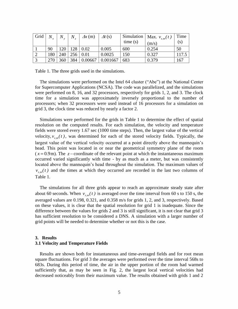
Grid xN yN

zN x (m) t (s) Simulation

time (s) Max. )t(v m,z

(m/s)

Time

(s)

1 90 120 128 0.02 0.005 600 0.254 50

2 180 240 256 0.01 0.0025 150 0.327 117.5

3 270 360 384 0.00667 0.001667 683 0.379 167

Table 1. The three grids used in the simulations.

The simulations were performed on the Intel 64 cluster (“Abe”) at the National Center

for Supercomputer Applications (NCSA). The code was parallelized, and the simulations

were performed on 8, 16, and 32 processors, respectively for grids 1, 2, and 3. The clock

time for a simulation was approximately inversely proportional to the number of

processors; when 32 processors were used instead of 16 processors for a simulation on

grid 3, the clock time was reduced by nearly a factor 2.

Simulations were performed for the grids in Table 1 to determine the effect of spatial

resolution on the computed results. For each simulation, the velocity and temperature

fields were stored every 1.67 sec (1000 time steps). Then, the largest value of the vertical

velocity, )t(v m,z , was determined for each of the stored velocity fields. Typically, the

largest value of the vertical velocity occurred at a point directly above the mannequin’s

head. This point was located in or near the geometrical symmetry plane of the room

( 90.x m). The z coordinate of the relevant point at which the instantaneous maximum

occurred varied significantly with time - by as much as a meter, but was consistently

located above the mannequin’s head throughout the simulation. The maximum values of

)t(v m,z and the times at which they occurred are recorded in the last two columns of

Table 1.

The simulations for all three grids appear to reach an approximate steady state after

about 60 seconds. When )t(v m,z is averaged over the time interval from 60 s to 150 s, the

averaged values are 0.198, 0.321, and 0.358 m/s for grids 1, 2, and 3, respectively. Based

on these values, it is clear that the spatial resolution for grid 1 is inadequate. Since the

difference between the values for grids 2 and 3 is still significant, it is not clear that grid 3

has sufficient resolution to be considered a DNS. A simulation with a larger number of

grid points will be needed to determine whether or not this is the case.

3. Results

3.1 Velocity and Temperature Fields

Results are shown both for instantaneous and time-averaged fields and for root mean

square fluctuations. For grid 3 the averages were performed over the time interval 568s to

683s. During this period of time, the air in the upper portion of the room had warmed

sufficiently that, as may be seen in Fig. 2, the largest local vertical velocities had

decreased noticeably from their maximum value. The results obtained with grids 1 and 2

6

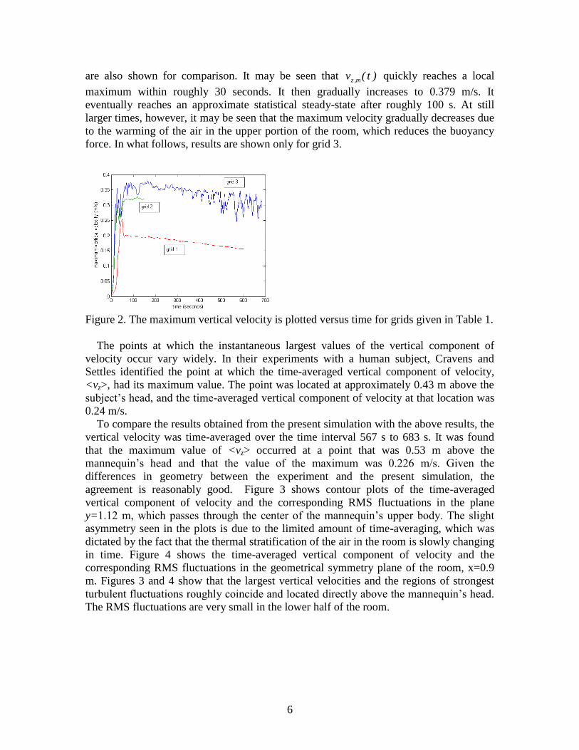
are also shown for comparison. It may be seen that )t(v m,z quickly reaches a local

maximum within roughly 30 seconds. It then gradually increases to 0.379 m/s. It

eventually reaches an approximate statistical steady-state after roughly 100 s. At still

larger times, however, it may be seen that the maximum velocity gradually decreases due

to the warming of the air in the upper portion of the room, which reduces the buoyancy

force. In what follows, results are shown only for grid 3.

Figure 2. The maximum vertical velocity is plotted versus time for grids given in Table 1.

The points at which the instantaneous largest values of the vertical component of

velocity occur vary widely. In their experiments with a human subject, Cravens and

Settles identified the point at which the time-averaged vertical component of velocity,

<vz>, had its maximum value. The point was located at approximately 0.43 m above the

subject’s head, and the time-averaged vertical component of velocity at that location was

0.24 m/s.

To compare the results obtained from the present simulation with the above results, the

vertical velocity was time-averaged over the time interval 567 s to 683 s. It was found

that the maximum value of <vz> occurred at a point that was 0.53 m above the

mannequin’s head and that the value of the maximum was 0.226 m/s. Given the

differences in geometry between the experiment and the present simulation, the

agreement is reasonably good. Figure 3 shows contour plots of the time-averaged

vertical component of velocity and the corresponding RMS fluctuations in the plane

y=1.12 m, which passes through the center of the mannequin’s upper body. The slight

asymmetry seen in the plots is due to the limited amount of time-averaging, which was

dictated by the fact that the thermal stratification of the air in the room is slowly changing

in time. Figure 4 shows the time-averaged vertical component of velocity and the

corresponding RMS fluctuations in the geometrical symmetry plane of the room, x=0.9

m. Figures 3 and 4 show that the largest vertical velocities and the regions of strongest

turbulent fluctuations roughly coincide and located directly above the mannequin’s head.

The RMS fluctuations are very small in the lower half of the room.

7

(a) (b)

Figure 3. The time-averaged vertical component of velocity (a) and the RMS fluctuations

in the vertical component of velocity (b) are shown in the plane y=1.12 m.

(a) (b)

Figure 4. The time-averaged vertical component of velocity (a) and the RMS fluctuations

in the vertical component of velocity (b) are shown in the plane x=0.9 m.

In Fig. 5, vz(t) is plotted over the time 567 s to 683 s at three points in the symmetry

plane of the mannequin shown in Fig. 3. The points are located along the symmetry line

at z= 1.50, 1.77, and 2.11 m. The corresponding distances above the mannequin’s head

are 0.26, 0.53 and 0.87 m. The second of the above points is the location at which the

time-averaged vertical component of velocity has its maximum value. For reference, the

ceiling is located at z= 2.45 m (1.21 m above the mannequin’s head.)

8

Figure 5. The instantaneous vertical component of velocity, vz(t), is plotted as a function

of time at three points above the mannequin’s head.

Figure 6 shows the instantaneous velocity field at 4143.t s in the geometrical

symmetry plane of the room ( 90.x m.) and the plane 121.y m, which passes through

the torso and head of the mannequin. Only 1/9 of the vectors are shown for clarity. It

may be seen that the flow is relatively complex in the region above the mannequin and

much smoother in the lower part of the room, which is consistent with the behavior of the

RMS fluctuations shown in Figs. 3 and 4.

(a) (b)

Figure 6. The instantaneous velocity at t = 143.s is shown in the planes (a) x=0.9m and

(b) y =1.12 m.

Figure 7 shows the time average temperature field and the RMS temperature

fluctuations in the plane x = 0.9m. It may be seen that the largest temperatures and RMS

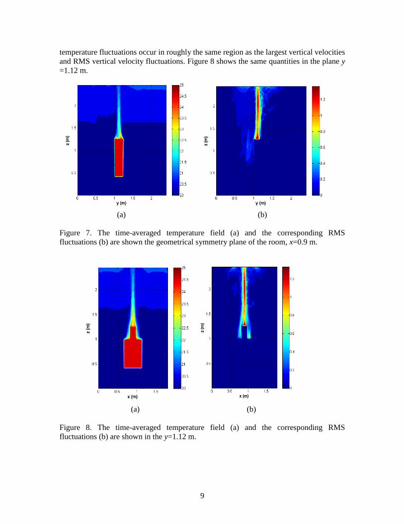
9

temperature fluctuations occur in roughly the same region as the largest vertical velocities

and RMS vertical velocity fluctuations. Figure 8 shows the same quantities in the plane y

=1.12 m.

(a) (b)

Figure 7. The time-averaged temperature field (a) and the corresponding RMS

fluctuations (b) are shown the geometrical symmetry plane of the room, x=0.9 m.

(a) (b)

Figure 8. The time-averaged temperature field (a) and the corresponding RMS

fluctuations (b) are shown in the y=1.12 m.

10

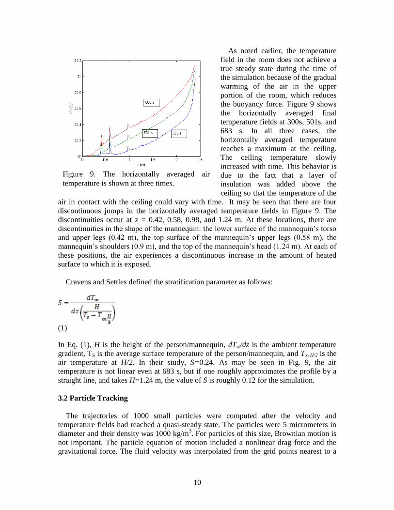
Figure 9. The horizontally averaged air

temperature is shown at three times.

As noted earlier, the temperature

field in the room does not achieve a

true steady state during the time of

the simulation because of the gradual

warming of the air in the upper

portion of the room, which reduces

the buoyancy force. Figure 9 shows

the horizontally averaged final

temperature fields at 300s, 501s, and

683 s. In all three cases, the

horizontally averaged temperature

reaches a maximum at the ceiling.

The ceiling temperature slowly

increased with time. This behavior is

due to the fact that a layer of

insulation was added above the

ceiling so that the temperature of the

air in contact with the ceiling could vary with time. It may be seen that there are four

discontinuous jumps in the horizontally averaged temperature fields in Figure 9. The

discontinuities occur at z = 0.42, 0.58, 0.98, and 1.24 m. At these locations, there are

discontinuities in the shape of the mannequin: the lower surface of the mannequin’s torso

and upper legs (0.42 m), the top surface of the mannequin’s upper legs (0.58 m), the

mannequin’s shoulders (0.9 m), and the top of the mannequin’s head (1.24 m). At each of

these positions, the air experiences a discontinuous increase in the amount of heated

surface to which it is exposed.

Cravens and Settles defined the stratification parameter as follows:

(1)

In Eq. (1), H is the height of the person/mannequin, dT∞/dz is the ambient temperature

gradient, TS is the average surface temperature of the person/mannequin, and T∞,H/2 is the

air temperature at H/2. In their study, S=0.24. As may be seen in Fig. 9, the air

temperature is not linear even at 683 s, but if one roughly approximates the profile by a

straight line, and takes H=1.24 m, the value of S is roughly 0.12 for the simulation.

3.2 Particle Tracking

The trajectories of 1000 small particles were computed after the velocity and

temperature fields had reached a quasi-steady state. The particles were 5 micrometers in

diameter and their density was 1000 kg/m3. For particles of this size, Brownian motion is

not important. The particle equation of motion included a nonlinear drag force and the

gravitational force. The fluid velocity was interpolated from the grid points nearest to a

11

(a) (b)

(c) (d)

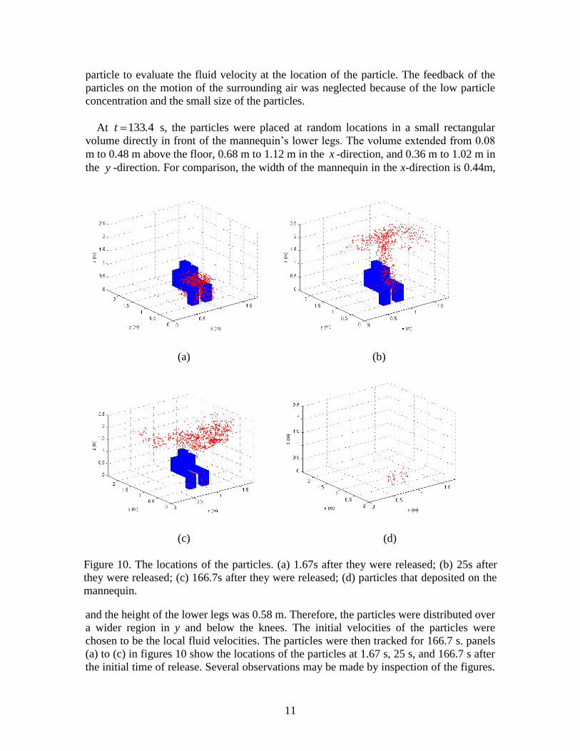
Figure 10. The locations of the particles. (a) 1.67s after they were released; (b) 25s after

they were released; (c) 166.7s after they were released; (d) particles that deposited on the

mannequin.

particle to evaluate the fluid velocity at the location of the particle. The feedback of the

particles on the motion of the surrounding air was neglected because of the low particle

concentration and the small size of the particles.

At 4133.t s, the particles were placed at random locations in a small rectangular

volume directly in front of the mannequin’s lower legs. The volume extended from 0.08

m to 0.48 m above the floor, 0.68 m to 1.12 m in the x -direction, and 0.36 m to 1.02 m in

the y -direction. For comparison, the width of the mannequin in the x-direction is 0.44m,

and the height of the lower legs was 0.58 m. Therefore, the particles were distributed over

a wider region in y and below the knees. The initial velocities of the particles were

chosen to be the local fluid velocities. The particles were then tracked for 166.7 s. panels

(a) to (c) in figures 10 show the locations of the particles at 1.67 s, 25 s, and 166.7 s after

the initial time of release. Several observations may be made by inspection of the figures.

12

First, it may be seen that the flow is effective in carrying the particles upward and also

drawing them toward the geometrical symmetry plane of the room (y=1.2 m) - particles

near the edges of the initial volume in the x -direction are drawn inward and upward by

the flow. This pumping action brings most of the particles, including particles that were

initially close to the floor, upward to the mannequin’s torso. In panel (b), it may be seen

that the majority of the particles are close to the ceiling due to the action of the thermal

plume. Some of the particles (38 out of 1000), however, deposit on the mannequin’s

lower legs and knees; the locations of these particles are shown in panel (d). Since

breathing was not included in the simulation, it is not possible to determine how many of

the particles would have been inhaled by the mannequin. Another striking feature of the

particle distribution in panel (c) is the broad range over which particles are dispersed in

the region near the ceiling.

4. Conclusions

Simulation results for the velocity and temperature fields inside a small room

containing a heated mannequin have been presented in this paper. The results were

obtained on a uniform spatial grid using a LBM. Results were obtained on three grids.

The results obtained on the finest grid (grid space equal to 0.00667 m) agree well with

results obtained by Craven and Settles in their experiments with a human subject.

Specifically, the maximum values of the time-averaged vertical component of velocity

for the simulation and the experiment were 0.226 m/s and 0.24 m/s, respectively. These

values were located at 0.53 m and 0.43 m above the mannequin’s head, respectively. The

stratification parameter was roughly the same as the experimental value for the period of

time in which the time averaging was performed for the simulation. Some of the

discrepancies may be due to differences in geometry: a standing human subject in a large

room versus an idealized model of a mannequin seated in a small room.

It is not clear that the results obtained on the highest resolution grid (grid 3) are grid

independent. Further study will be needed to determine the requirements for grid

independence. The values of the instantaneous global maximum for the vertical

component of velocity show significant differences for grids 2 and 3. It is, however, true

that, at larger times, the vertical velocities decrease substantially and this would

presumably decrease the requirements for accurate simulations because the Reynolds

number is smaller.

It is likely that the number of grid points could be reduced by a significant factor by

using a coarser grid in the lower half of the room and in some portions of the upper half

of the room. A fine grid would still be needed near the mannequin to resolve the thermal

boundary layer. It would be more straightforward to implement such a variable grid using

alternate numerical simulation techniques such as the finite volume method.

The results obtained by tracking 5 micrometer particles from a small volume near the

floor and in front of the mannequin suggest that the mannequin’s thermal plume is quite

effective at bringing small particles close to the mannequin. A small fraction (~4%) of

13

the particles deposited on the mannequin’s lower legs during the simulation. Most of the

remaining particles were distributed over a broad area near the ceiling at the end of the

simulation. A longer simulation would be needed to determine how many of these

particles deposit on the mannequin. It is expected that results for longer times as well as

higher spatial and temporal resolution will be reported elsewhere.

Acknowlegements

The authors wish to acknowledge support for this work from the Syracuse Center of

Excellence CARTI Program. The authors gratefully acknowledge the support and

facilities of the NCSA at the University of Illinois.

References

[1] B. Cravens, G.S. Settles, A computational and experimental investigation of the

human thermal plume, J. Fluids Eng. 128 (2006) 1251-1258.

[2] F.P. Incropera, D.P. DeWitt, Fundamentals of Heat and Mass Transfer, Wiley, New

York, 2002.

[3] D. Marr, Velocity measurements in the breathing zone of a moving thermal manikin

within the indoor environment, Ph.D. thesis, Syracuse University, 2007.

[4] D.R. Marr, I.M. Spitzer, M.N. Glauser, Anisotropy in the breathing zone of a

thermal manikin, Exp. Fluids 44, (2008) 661-673.

[5] I.M. Spitzer, I.M., D.R. Marr, M.N. Glauser, Impact of manikin motion on particle

transport in the breathing zone, J. Aerosol Sci. 41 (2010) 373-383.

[6] A.M. Abdilghanie, L.R. Collins, D.A. Caughey, Comparison of turbulence

modeling strategies for indoor flows, J. Fluids Eng. 131 (2009) 051402-1.

[7] L. Davidson, P.V. Nielsen, Large eddy simulation of the flow in three-dimensional

ventilated room, Proceedings of the Fifth International Conference on Air

Distribution in Rooms, Yokohama, Japan (1996) 161-168.

[8] W. Zhang, Q. Chen, Large eddy simulation of indoor airflow with a filtered

dynamic subgrid scale model, Int. J. Heat Mass Transfer 43 (2000) 3219-3231.

[9] W. Zhang, Q. Chen, Large eddy simulation of natural and mixed convection airflow

indoors with two simple filtered dynamic subgrid scale models, Num. Heat Transfer

A 37 (2000) 447-463.

[10] Y. Jiang, Q. Chen, Using large eddy simulation to study air-flows in and around

buildings, ASHRAE Trans. 109 (2003) 517-526.

[11] T. Inamuro, T. Ogata, S. Tajima, N. Konishi, A lattice Boltzmann method for

incompressible two-phase flows with large density differences, J. Comp. Phys. 198

(2004) 628-644.

[12] T. Inamuro, M. Yoshino, H. Inoue, R. Mizuno, F. Ogino, A lattice Boltzmann

method for a binary miscible fluid mixture and its application to a heat-transfer

problem, J. Comp. Phys. 179 (2002) 201-215.

[13] X. He, S. Chen, G.D. Doolen, A novel thermal model for the lattice Boltzmann

method in incompressible limit, J. Comput. Phys. 146 (1998) 282.

14

[14] P. Lallemand, L.S. Luo, Hybrid finite-difference thermal lattice Boltzmann

equation, Int. J. Modern Phys. B 17 (2003) 41.

[15] P. Lallemand, L.S. Luo, Theory of the lattice Boltzmann method: Acoustic and

thermal properties in two and three dimensions, Phys. Rev. E. 68 (2003) 036706.

[16] C.S. Nor Azwadi, T. Tanahashi, Development of 2-D and 3-D double population

thermal lattice Boltzmann models, Matematika 24 (2008) 53-66.

[17] C-H Liu, K-H Lin, H-C Mai, C-A Lin, Thermal boundary conditions for thermal

lattice Boltzmann simulations, CAMWA 59 (2010) 2178-2193.

[18] J. Derksen, H.E.A. Van den Akker, Large eddy simulations on the flow driven by a

Rushton impeller, AIChE J. 45 (1999) 209-221.