Simulation and Measurement of Radio Wave Propagation … · DEPARTMENT OF ELECTROSCIENCE LUND INSTITUTE OF TECHNOLOGY SWEDEN Simulation and Measurement of Radio Wave Propagation in

Department of Electroscience

Master of Science Thesis Luz Bruno Picasso & Patrick Jansson

in cooperation withSt. Jude Medical

February 2004

Simulation and Measurement of Radio WavePropagation in the 400 MHz MICS Band

DEPARTMENT OF ELECTROSCIENCE

LUND INSTITUTE OF TECHNOLOGY

SWEDEN

Simulation and Measurement of Radio Wave

Propagation in the 400 MHz MICS Band

Master of Science Thesis

By

Luz Bruno Picasso, Patrick Jansson

Supervisor:

Anders J Johansson, Department of Electroscience, Lund

April 2004

Wave-Propagation in the 400MHz MICS band

Luz Bruno Picasso, Patrick Jansson Version 1.0 3 of 3

Abstract

The pacemaker is today, forty-five years after its invention, a common implant. The ability to communicate with a medical implant such as the pacemaker is desirable since it then may be programmed and adapted to the varying health condition of the patient.

This thesis investigates the propagation and interference pattern of a dipole antenna at 403.5 MHz in an indoor environment. Measurement series were taken in order to identify communication problems due to these phenomena. The measurements show that correct polarisation and the positioning of the antennas are essential for good signal reception.

Simulations made in the computer tool SEMCAD are compared to the measurements and the ability of the program to reflect reality is evaluated. Measurements and simulations agree regarding attenuation and variations in propagation loss. Interference patterns in SEMCAD differ from measurements since the reflection characteristics depend on frequency dependent material parameters of the walls that are difficult to obtain.

Further areas for study to achieve a viable solution are discussed. Suggestions to increase signal reception include transmitting with two different antennas and with varying polarisations for best signal reception.


4 of 4 Version 1.0 Luz Bruno Picasso, Patrick Jansson



Contents

Abstract ................................................................................................................................3

Contents................................................................................................................................5

1 Background...................................................................................................................7

1.1 Technical history ....................................................................................................7

1.2 The concept for this thesis.......................................................................................9

2 Software – PB-FDTD..................................................................................................11

2.1 Introduction to FDTD ...........................................................................................11

2.2 Modelling and simulation of an dipole antenna .....................................................13

3 Software – SEMCAD..................................................................................................16

3.1 Modelling and simulation of a dipole antenna in a “hospital room” .......................16

3.2 Results..................................................................................................................19

4 Antenna design and verification ................................................................................23

5 Measurements.............................................................................................................28

5.1 Measurements of a dipole antenna in a room.........................................................28

5.2 Results..................................................................................................................33

6 Results: Comparing between theory and reality .......................................................44

7 Conclusions .................................................................................................................48

8 Discussion....................................................................................................................49

9 References ...................................................................................................................50

Appendix A - Simulation diagrams ...............................................................................51

Appendix B - Antenna radiation patterns.....................................................................54

Appendix C - Measurement diagrams...........................................................................55





1 Background

1.1 Technical history

In 1958 Dr Senning and Dr Elmqvist in Stockholm, Sweden, were the first to correct heart arrhythmias with an implanted pacemaker [1]. The device required implantation to reduce the risk of infection and therefore had to be small enough to implant subcutaneously. This pacemaker was recharged with induction [2]. An external charger unit generates a power transfer by 150 kHz mutual induction. The charger coil is placed on the skin of the patient over the pacemaker where another coil is within the implanted generator. The pacemaker of Dr. Rune Elmqvist is shown in Figure 1. This technique is still the basis of what is used today to reprogram and extract information from modern pacemakers.

Figure 1 - The first implantable pacemaker

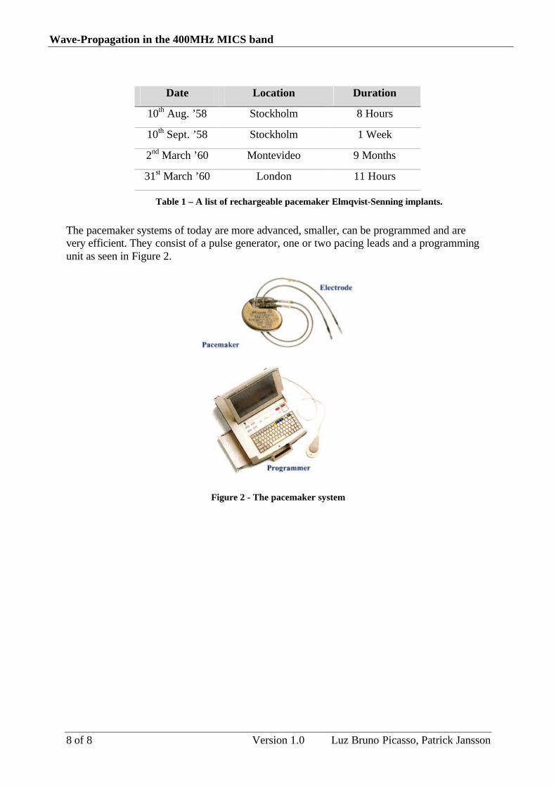
Arne Larsson was the first patient in the world to receive a completely implantable pacemaker in 1958. This first pacemaker had to be recharged after eight hours due to leakage of the battery acid. The rapid development of silicon transistors, requiring less power and space, highlighted the choice of batteries as the most important factor in the effort to increase time between chargings. The preferred choice fell to nickel-cadmium rechargeable cells. In February 1960 a team led by Dr Fiandra and Dr Rubio in Uruguay implanted the same pacemaker, now with new rechargeable batteries [2]. It was envisioned that the patient would not need to charge the battery for a long time. She died nine months after the implantation due to an infection. In Table 1 the first rechargeable pacemakers and the duration of the batteries are listed [2].



Date Location Duration

10th Aug. ’58 Stockholm 8 Hours

10th Sept. ’58 Stockholm 1 Week

2nd March ’60 Montevideo 9 Months

31st March ’60 London 11 Hours

Table 1 – A list of rechargeable pacemaker Elmqvist-Senning implants.

The pacemaker systems of today are more advanced, smaller, can be programmed and are very efficient. They consist of a pulse generator, one or two pacing leads and a programming unit as seen in Figure 2.

Figure 2 - The pacemaker system



The positioning of the implants in the thorax is pictured in Figure 3.

Figure 3 - Pacemaker implants

Another pioneer in the development of pacemakers was Wilson Greatbach, an American radio engineer. While working on a circuit to record fast heart sounds he, accidentally, used an incorrect transistor, which caused the circuit to pulse. Greatbach recognized the sound as the correct rhythm of a heart. Assisted by two Americans surgeons, Gage and Chardak, a device for controlling heart beats was built and tested on a dog. This first attempt was successful and Dr Chardak performed the first operation on a human patient in April 1960, [3].

1.2 The concept for this thesis

A new frequency range, from 402 MHz to 405 MHz, has been assigned for medical implants. The task has been to investigate the propagation pattern of the near field of electromagnetic waves in a small room and to determine whether this behaviour causes difficulties in the communication between two devices. The most basic radio wave propagation model is the “free space” radio propagation. In this model, radio waves emanate from a point source of power, travelling in all directions in a straight line, filling the entire spherical volume of space with power. The power received decreases proportionally to 1/r2, r being the distance. Of course this model rarely describes the actual propagation accurately; phenomena such as reflection, diffraction and scattering exist that disturb radio propagation. These cause signal variations and further contribute to signal propagation losses.

The aim is to analyse and identify communication problems due to this propagation and suggest solutions or further areas for study to achieve viable solutions. An evaluation of the ability of the SEMCAD simulation tool to reflect reality and how the results comply with field measurements is included.

Therefore the antenna was first simulated in a virtual room. The measurements were conducted in an actual room (referred to as the “hospital room”) which is in the cellar at the Institute of Technology in Lund (house E, room 0412), see Figure 4.



Computer simulations were made using two different computer programs; PB-FDTD [7] and SEMCAD [4].

Figure 4 – CAD model of the simulated and measured “hospital room”.



2 Software – PB-FDTD

2.1 Introduction to FDTD

One technique for simulating antennas is the Finite-Difference-Time-Domain (FDTD) [5].

This powerful numerical method was developed to solve electromagnetic problems based on a second order finite-difference approximation of the partial derivatives in Maxwell’s equations and was developed by Kane S. Yee (1966) [6]. Maxwell’s two equations can thus simultaneously be solved for the E- and the H field.

( ) ( ) ( ) ( )[ ]2,,2/1,2/1),,,xO

xkjiFkiF

xnkjiF nn

∆∆

−−+=

∂∂

(1)

( ) ( ) ( ) ( )[ ]22/12/1 ,,,,),,,

tOt

kjiFkjiFt

nkjiF nn

∆∆−

=∂

∂ −+

(2)

In equations (1) and (2)

Fn is the E or H- field at time n⋅∆t.

i, j, k are indices of the spatial lattice.

O[(∆x)2] and O[(∆t)2] are the error terms.

The following two differences apply to Maxwell’s curl equations

HH

tE

EEt

H

H

E

σµ

σε

−∂∂

−=×∇

+∂∂

=×∇

(3)

where σE and σH are the electric and the magnetic losses.

These two equations lead to the following equation for Ex (the corresponding equations for Ey, Ez, Hx, Hy and Hz are calculated analogously).

−

∆

−−

∆

−=

∆

−+

+−

++

+−

++

+2/1

,,,,

2/12/1,,

2/12/1,,

2/1,2/1,

2/1,2/1,

,,

,,1,, 1 n

kjixkji

nkjiy

nkjiy

nkjiz

nkjiz

kji

nkji

nkjix E

z

HH

y

HH

t

EEσ

ε(4)



Assuming the approximation

2,,

1,,2/1

,,

nkjix

nkjixn

kjix

EEE

+=

+

+ , (5)

the latest equation can be reduced to the unknown

.1

21

21 2/1

2/1,,2/1

2/1,,2/1

,2/1,2/1

,2/1,

,,

,,

,,,,

,,

,,

,,

,,

1,,

∆

−−

∆

−

∆+

∆

+

∆+

∆−

=+

−+

++

−+

++

z

HH

y

HH

t

t

Et

t

En

kjiyn

kjiyn

kjizn

kjiz

kji

kji

kjinkjix

kji

kji

kji

kji

nkjix

ε

σε

ε

σε

σ

(6)

All this leads to six equations for each cube in the lattice (the FDTD method divides space into a lattice of Yee cells). The Yell cell, seen in Figure 5, contains three electric field components and three magnetic field components and describes how the field components should be oriented (one E-field component is surrounded by two H-field components perpendicular to the E-field).

Thus the method is robust, flexible and easy to implement, but it is computationally intensive.

The fact that it is computationally intensive is due to numerical dispersion (when the analytical phase velocity differs from the simulated) under certain stability conditions. In order to decrease the numerical dispersion the FDTD, the cell sizes have to be small, no larger than one tenth of a wavelength.

Figure 5 - The Yee cell



The FDTD time step ∆t, used in the calculations, depends on the size of the Yee cell and is given by

222

11199,0

zyxc

t

∆+

∆+

∆

=∆ (7)

where c is the speed of light in vacuum.

∆x, ∆y, ∆z are the length of the sides of the Yee cell.

The use of small cells results in short simulation time steps, which increases the number of simulation steps and the computational time. The more complex the environment (higher resolutions) required to be simulated, the smaller the cell required. However this goes towards a shorter step time. This in turn leads to compromises between the run time and the geometrical demands.

2.2 Modelling and simulation of an dipole antenna

Simulation of the dipole antenna was conducted using PB-FDTD (Periodic-Boundary-Finite-Difference-Time-Domain) software [7]. Henrik Holter developed this while a Ph.D. student at the Royal Institute of Technology in Stockholm. As the name implies, the underlying technique is FDTD. Periodic boundary conditions are implemented to reduce the computational volume of periodic structures to a single periodic cell.

There are seven different types of simulation available in the PB-FDTD software. The choice in this case is the ordinary FDTD which is the standard FDTD with absorbing boundaries conditions (ABC) on all six boundaries (with no periodic boundaries). This means that the field does not radiate back into the adjacent cells, the final cells absorb all the energy.

The first iteration was done by drawing a dipole antenna which is one of the most widely used antennas for wireless communication systems, see Figure 6. The excitation pulse is a sinusoidal modulated Gaussian pulse.



Figure 6 - Dipole antenna

Since

m

fc

743.010*5,40310*8,299

6

6

===λ . (8)

The ideal half wavelength dipole should be ?/2 = 0.372 m.

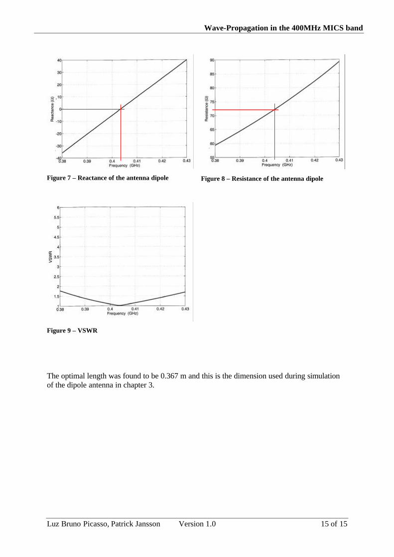
The feed impedance was 50 Ω. In order to push the antenna to resonate the length must be shortened as the input impedance needs to be real, see Figure 7 and Figure 8 (see chapter 4 for in-depth detail). The length was empirically determined by shortening the length until the Voltage Standing Wave Ratio was optimised (VSWR = 1) see Figure 9. This is the value when a perfect match is obtained and no reflections appear which leads to all of the power being transmitted. VSWR describes the ratio of the maximum value of the electric field intensity of a standing wave.



Figure 7 – Reactance of the antenna dipole

Figure 8 – Resistance of the antenna dipole

Figure 9 – VSWR

The optimal length was found to be 0.367 m and this is the dimension used during simulation of the dipole antenna in chapter 3.



3 Software – SEMCAD

3.1 Modelling and simulation of a dipole antenna in a “hospital room”

Chapter 3 focuses on the software package for electromagnetic simulation, SEMCAD (Simulation Platform for Electromagnetic Compatibility, Antenna Design and Dosimetry) [8]. This is a very powerful program and requires a high performance PC with large a memory.

The model was constructed as a room (3440 x 2280 x 3020 mm) identical to that where the physical measurements were planned, sparsely furnitured with a bed, a desk, a chair and a dipole antenna with the length calculated in chapter 2.2. The room, as a CAD model, can be seen in Figure 10. On completion of the model the simulation mode was activated with the chosen cell grids and the boundary type as ABC (Absorbing boundary Conditions). All the materials in the model were defined with the corresponding parameters, such as concrete in the walls, wood in the bed and chair and metal modelled as PEC, Perfect Electric Conductor. Examples are shown in Table 2 and Table 3 .In Figure 11 the simulated room is shown with propagation in the YZ-plane.

Material Relative permittivity, εr

Relative permeability µr

Conductivity σE [S/m]

Source

Concrete 6 1 0.01 [9]

Gypsum 4 1 1e-2 [10]

Wood 2.3 1 2 e-11 [10]

Metal 0 1 PEC

Glass 5.5 1 1 e-12 [11]

Table 2 - Material Parameters



Object Name Material

Wall (to the outside) Concrete

Wall (to the toilet) Gypsum

Wall (to the corridor) Gypsum

Wall Gypsum

Ceiling Concrete

Floor Concrete

Bed Wood

Table frame Metal

Table surface Wood

Table legs Metal

Chair Wood

Ladder Metal

Toilet door Wood

Corridor door Wood

Ventilation shaft Metal

Windows glass Glass

Radiator Metal

Table 3 - Materials of simulated objects



Figure 10 - Simulated “Hospital room” in SEMCAD

Figure 11 - Simulated “Hospital room” in SEMCAD showing propagation in YZ-plane



Simulation path Transmitting antenna Receiving antenna

Polarisation Height, mm (Z-direction)


Unfurnished

SA: Along Y-axis Vertical 1050 Vertical 1050

SB: Along Y-axis Vertical 1050 Horizontal 1050

SC: Along Y-axis Vertical 1050 Z 1050

Furnished

SJ: Along Y-axis Vertical 1050 Vertical 1050

SK: Along Y-axis Vertical 1050 Horizontal 1050

SP: Area above the bed Vertical 1050 Vertical 660

Table 4 - Table over the simulated path

3.2 Results

The value SEMCAD provides is in dB (V/m) = dB [E] = 10 * log (E2), and the power is

22

** λeair

in AZE

P = , (9)

where Z is the impedance,

Ae the effective antenna area

and λ the wavelength.

Therefore the simulated value from SEMCAD is comparable to the values measured later including a constant. The constant is calculated by

( ) ( )222

22

22

log*10log*10*

log*10**log*10** ECEZ

AA

ZE

AZE

Pair

ee

aire

airin +=+

=

⇒=

λλλ (10)



This constant has however not been calculated here as the constant A is required in the formula for the simulation to be entirely correct. The correct formula therefore should be

22

*** λeair

in AAZE

P = , (11)

where A depends on how the antenna has been simulated. After comparing the measurements to the simulations it was decided to add an offset of 27 dB to the simulated values. The decision to use 27 dB was resulted from comparing measurement A and simulation SA in Figure 35. All simulated values in this thesis contain this offset value.

Graphs of all simulations are individually presented in Appendix A.

-120

-100

-80

-60

-40

-20

0

20

-150 -100 -50 0 50 100 150 200 250 300

Distance from transmitting antenna [cm]

Pro

pag

atio

n lo

ss [

dB

]

Propagation loss [dB], simulation SA

Propagation loss [dB], simulation SB

Propagation loss [dB], simulation SC

Figure 12 - Transmitting antenna vertically polarised with various polarisations of receiving antenna in an unfurnished room. Simulations SA, SB, SC

The simulations in Figure 12 indicate that large differences in attenuation can be anticipated between different polarisations. The simulated values are at their highest close to the antenna and abruptly fall as they approach the wall; also the co-polarised signal indicates the best receiving quality as expected.



-120

-110

-100

-90

-80

-70

-60

-50

-40

-30

-20

-150 -100 -50 0 50 100 150 200 250 300


Pro

pag

atio

n lo

ss [

dB

]

Propagation loss [dB], simulation SJ

Propagation loss [dB], simulation SK

Figure 13 - Transmitting antenna vertically polarised with various polarisations of the receiving antenna in a furnished room. Simulations SJ and SK

The simulations in Figure 13 show that, regardless of polarisation, the attenuation is evenly high. The signal is highly attenuated even at the antenna position and does not reach higher values than -50 dB anywhere in the series. SEMCAD does not give us values for SK all the way to the wall; further investigation of this is however outside the scope of this study.



Figure 14 - Simulation of the entire room 660 mm above the floor. SP is a subset of this simulation. Both transmitting and receiving antennas are vertically polarised.

Simulating the area over the bed SEMCAD requires an entire cross-section of the room to be captured as in Figure 14. The interference between different reflections of the propagation can clearly be identified here. The power decrease of the signal when it is transmitted into a concrete wall is especially visible in the right area of the figure. The area of particular interest is a subset of this cross-section and in chapter 6 this has been extracted from the image for closer comparison with the measurements.

SP

Desk



4 Antenna design and verification

The chosen antenna type for this project is a standard half wavelength dipole. The reason for this is that it is an easy antenna to construct and verify. As we wish to operate in the frequency span 402-405 MHz the antenna is designed to resonate at the centre frequency of 403.5 MHz with a bandwidth of 3 MHz or 0.7%. Using hollow cylindrical brass antenna arms a length to diameter ratio of 5000 is required for 3% bandwidth [12]. The higher the L/d ratio is the greater bandwidth the antenna has. Since the length is

m

c3717.0

10*5.403*22 6≈=

λ

(12)

we need to use arms of at least d = 0.07 mm. Choosing arms of d = 4 mm exceeds meets these requirements. These calculations are made considering homogenous cylindrical antenna arms, however they may be used in this case due to the skin effect, i.e. the current will only travel in the periphery of the arms [13].

A dipole antenna has an impedance of (73.05 +j42.55) O [12], [14]. But for the antenna not to reflect any power it has to resonate i.e. it has to have real impedance. The easiest way to achieve this is by measuring the antennas VSWR and shorten the antenna arms until optimal VSWR = 1 is reached and the antenna resonates. VSWR is the Voltage Standing Wave Ratio and defined by

Γ−Γ+

=1

1VSWR

(13)

where

0

0

ZZZZ

L

L

+−

=Γ

(14)

and ZL and Z0 are the impedances for the antenna feed and the antenna itself respectively. The feed to the antenna was a coaxial cable with ZL = 50 O (2.2 mm in diameter) and a soldered SMA-plug. The VSWR was measured with a network analyser (Rohde & Schwarz ZVC) and the antenna was shortened until it was optimised, resulting in a length of 340 mm.

When constructing a dipole antenna with this design one has to bear in mind that the inner and outer conductor of the coaxial cable are not connected to the antenna arms in the same way and thus the antenna feed is unbalanced. The unbalance is caused by a current flow to ground on the outside of the outer conductor, leaving the antenna arms with an unequal feed as shown in Figure 15. An unbalanced dipole antenna does not have the classical half wavelength dipole radiation pattern and is asymmetric in its radiation due to the current flowing on the outside of the line feed [15].



I2 I3I2-I3

I1

I2-I3

I3

I2 I1

#2 #1

Zg

ZL

?/2

I1

Figure 15 - Unbalanced coaxial line and its electrical equivalent

The solution to balancing the antenna is called a balun (balance to unbalance). There are several types of baluns to choose from depending on the application [16]. By reason of simplicity and efficiency the bazooka balun was chosen for this project [12], [16], [17]. The bazooka balun consists of a quarter wavelength metal sleeve that is shortened to the outer coax conductor at one end as shown in Figure 16. In this way the current I3 will “see” a new transmission line with the coaxial feed being the inner conductor and the metal sleeve being the outer conductor.

?/2

Shorted tocoax’s outerconductor Coaxial line

Metal sleeve?/4

Figure 16 - Bazooka balun

Due to of the short to the coax’s outer conductor and since the length of the balun is ?/4 the input impedance of the new shortened transmission line will be infinitely high and therefore chokes the current flow and thus it will balance the antenna. This is the same effect as when



setting the impedance ZG in Figure 15 to infinity. This is calculated using the formula for the characteristic impedance of a transmission line,

( ) ( )( ) ( )ljZlZ

ljZlZZZ

L

L

ββββ

sincossincos

0

00 +

+= , (15)

where ß is 2p/?.

Since the length is ?/4 and

the short gives that ZL = 0, we conclude that

( )( ) ( ) ∞=

===

2tantan

cossin

000

00

πβ

ββ

jZljZlZljZ

ZZ . (16)

The current velocity in a coaxial cable is

r

vε

810*3= , (17)

where er is the dielectric constant of the medium [18].

Using this, the electrical wavelength in the balun and the length of the metal sleeve may be determined. The medium in this case is air, which means that er = 1 and the wavelength in the balun is the same as for free space. This leads to a sleeve length of 18.6 cm.

Due to the weight of the antenna arms, a plastic ring was fitted around the construction to provide a mechanical support. This was in turn fitted to a plastic tube which simplified the mounting of the antenna to a stand that was used for the measurements. The antenna, including structural parts, is shown in Figure 17.



Figure 17 - The half wavelength antenna, including plastic structures for mechanical support and

mounting.

Two of these antennas were built, one to transmit, and one to receive. In order to verify the antennas, their far-field radiation patterns were measured in an outdoor environment. This was done by sending 0 dBm from an antenna on the 1st floor level (some 5 meters above ground level) and receiving the signal in the grounds some 35 m away. Since the ground level area is sloped, the transmitting antenna is 5 meters from the ground and thus better simulates free space (Figure 18). Thus with over 40 wavelengths apart the measurement is carried out in the far-field (Fraunhofer) region. These measurements were done using a HP 8642B signal generator for sending and a HP 8519A spectrum analyser for receiving. All measurements are average values taken over a range of 100 values. As expected, when plotted in a polar plane the radiation patterns are kidney shaped. It is therefore concluded that the antennas work as balanced half wavelength dipoles. The polar plots of the signals received with the antennas are shown in Appendix B.

Basement

1:st floorParking lot

Transmitting antenna

Antenna under verification

Figure 18 - Sketch of the measurement set-up area when verifying the antennas. Being well off the ground

reduces interference due to reflections.



A third dipole antenna was also constructed. This antenna is identical in regard to electrical construction as the two previously built, with the exception of the length of the antenna arms. A length of 90 mm and width of 2 mm ensures that the antenna has the required bandwidth, but with an impedance of (1.8 + j4.9) O and a VSWR of 26 it does not resonate at 403.5 MHz. Since the size of this antenna is smaller mechanical support is not required. The purpose of this antenna was to investigate whether scattering from the antenna affected the propagation measurement.



5 Measurements

5.1 Measurements of a dipole antenna in a room

Measurements were taken in a room devoid of furniture that later was furnished to resemble a “typical” hospital room with a chair, desk, and bed as seen in Figure 4, chapter 1.2. The measurement points in the room were no more than 25 mm apart since 20 measurements per wavelength are required to avoid the necessity of using interpolation techniques, [19]. In order to accomplish this with an acceptable degree of accuracy, the floor was taped and marked with measuring points. The antennas were then fitted in rigid plastic stands whose markings were aligned with the markings on the floor as in Photo 1. After furnishing for phase 2 of the measurements, the transmitting antenna was placed on a small stand over the desk, thus maintaining the same coordinates (1050, 1050, 1050) as for the simulations and the measurements of the unfurnished room. This coordinate is identical to that used in the chapter on simulation.

Photo 1 - Antenna and stand, including stand markings and taped floor.

The instrumentation, a signal generator (HP 8642) for transmitting, and a spectrum analyser (Advantest R3131) for receiving, was placed in an adjacent room to minimise interference with the measurements. The instruments are shown in Photo 2, and the complete “link budget” of the set-up can be seen in Figure 19. The instrument settings were as follows: 0 dBm output power, 10 kHz RBW, 100kHz VBW, 50 ms SWP, 0 kHz span, and the measured values represent an average of 20 values.



Photo 2 - The Advantest R3131 spectrum analyser placed above the HP 8642B signal generator.

Figure 19 - “Link budget” of the measurement setup

All measurement results reported include antenna gain but exclude cable loss, i.e. -Lp + Gt + Gr. Thus the cable loss (11.6 dB + 5.4 dB) is added to the measured value for available input power, Ct. The gain must be included since it is an integral part of the dipole antenna. In the case other antenna types are used the interference and propagation patterns will differ.



Several series of measurements with the room, both furnished and unfurnished, were recorded to investigate various characteristics and phenomena of interest. These are presented in Table 5.

Measurement path Transmitting antenna Receiving antenna



Unfurnished

A: Along Y-axis Vertical 1050 Vertical 1050

B: Along Y-axis Vertical 1050 Horizontal 1050

C: Along Y-axis Vertical 1050 Z 1050

D: Along Y-axis Horizontal 1050 Horizontal 1050

E: Along Y-axis Horizontal 1050 Vertical 1050

F: Along Y-axis Horizontal 1050 Z 1050

G: Along Y-axis Vertical 1050 Vertical (Small antenna) 1050

H: 25° deviation from Y-axis in pos. X-direction

Vertical 1050 Vertical 1050

I: 25° deviation from Y-axis in neg. X-direction


Furnished

J: Along Y-axis Vertical 1050 Vertical 1050

K: Along Y-axis Vertical 1050 Horizontal 1050

L: Along Y-axis CO 45 1050 CO 45 1050

M: Along Y-axis CROSS 45 1050 CROSS 45 1050

N: 25° deviation from Y-axis in pos. X-direction


O: 25° deviation from Y-axis in neg. X-direction


P: Area above the bed Vertical 1050 Vertical 660

Q: NLOS meas. in neg. X-direction out to corridor


Table 5 – Results recorded over the measurement series.



Receiver antenna Polarisation Transmitter antenna

Co-polarisation

Co-polarisation

Cross-polarisation

Z polarisation

Co 45 polarisation

Cross 45 polarisation

Table 6 - Antenna polarisations

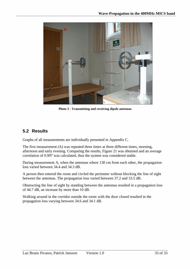
Z polarisation is when the antennas were placed with the receiving antenna arms parallel with the Y-axis. The transmitting and receiving antennas arms were in the XZ-plane for all measurements with exception of measurements C and F where the receiving antenna arms were parallel with the Y-axis. CO 45 polarisation is co-polarisation with both antennas rotated 45°, i.e. between vertical and horizontal polarisation. CROSS 45 polarisation is as CO 45, with one difference, that the antennas are rotated 45° in opposite directions and thus cross-polarised. Further clarification in Table 5, Table 6 shows the room including the measurement series and the various polarisations tested. Photo 3 shows the antennas during measurement J.



Figure 20 - Measured areas



Photo 3 - Transmitting and receiving dipole antennas

5.2 Results

Graphs of all measurements are individually presented in Appendix C.

The first measurement (A) was repeated three times at three different times, morning, afternoon and early evening. Comparing the results, Figure 21 was obtained and an average correlation of 0.997 was calculated, thus the system was considered stable.

During measurement A, when the antennas where 130 cm from each other, the propagation loss varied between 34.4 and 34.3 dB.

A person then entered the room and circled the perimeter without blocking the line of sight between the antennas. The propagation loss varied between 37.2 and 33.5 dB.

Obstructing the line of sight by standing between the antennas resulted in a propagation loss of 44.7 dB, an increase by more than 10 dB.

Walking around in the corridor outside the room with the door closed resulted in the propagation loss varying between 34.6 and 34.1 dB.



-40

-35

-30

-25

-20

-15

-10

-5

0

0 50 100 150 200 250


Pro

pag

atio

n lo

ss [

dB

]

Propagation loss [dB], 1:st A measurementPropagation loss [dB], 2:nd A measurementPropagation loss [dB], 3:rd A measurement

Figure 21 - Three different measurements type A with both antennas vertically polarised in an unfurnished room.

Comparing co-polarisation with different cross-polarisations, as in Figure 22 and Figure 23, the decrease of the power received when reception is a cross-polarised signal instead of a co-polarised signal is observed. Therefore the polarisation must be carefully considered for optimum signal reception.



-70,0000

-60,0000

-50,0000

-40,0000

-30,0000

-20,0000

-10,0000

0,0000

0,0 50,0 100,0 150,0 200,0 250,0


Pro

pag

atio

n lo

ss [

dB

]

Propagation loss [dB], measurement A

Propagation loss [dB], measurement B

Propagation loss [dB], measurement C

Figure 22 - Comparing measurements A, B and C. Transmitting antenna vertically polarised and the receiving antenna at various polarisations in an unfurnished room.

-70

-60

-50

-40

-30

-20

-10

0

0 50 100 150 200 250


Pro

pag

atio

n lo

ss [d

B]

Propagation loss [dB], measurement D

Propagation loss [dB], measurement EPropagation loss [dB], measurement F

Figure 23 - Comparing measurements D, E and F. Transmitting antenna horizontally polarised and various polarisations of receiving antenna in an unfurnished room.



Can any difference between vertical and horizontal co-polarisation be noted? Studying Figure 24 the interference patterns are slightly different, but the power variation levels are still comparable with the exception of the 150 cm distance. One hypothesis is that the waves are reflected differently for each polarisation.

-35

-30

-25

-20

-15

-10

-5

0

0 50 100 150 200 250


Pro

pag

atio

n lo

ss [

dB

]

Propagation loss [dB], measurement APropagation loss [dB], measurement D

Figure 24 - Comparing measurements A and D. Vertical (A) and horizontal (D) co-polarisation measured in an unfurnished room.

Using half wavelength dipoles as in this case, the antenna arms tend to get rather big at RF-frequencies. To investigate if the size caused scattering of the EM-waves and thus disturbed the signal reception a smaller antenna as discussed in chapter 4 was constructed. The comparison between these antenna sizes is seen in Figure 25. . The difference in received power is natural as the smaller antenna is not built for this frequency. The two measurements were compared by increasing the received power of the smaller antenna with 32 dB to compensate. The patterns are very similar and thus oppose any theories that scattering is a factor large enough to be considered. The cut-offs for the lowest values of the smaller antenna are due to signal disappearance below the noise floor.



-35

-30

-25

-20

-15

-10

-5

0

0 50 100 150 200 250


Pro

pag

atio

n lo

ss, m

easu

rem

ent

A [

dB

]

-67

-62

-57

-52

-47

-42

-37

-32

Pro

pag

atio

n lo

ss, m

easu

rem

ent

G [

dB

]

Propagation loss [dB], measurement APropagation loss [dB], measurement G

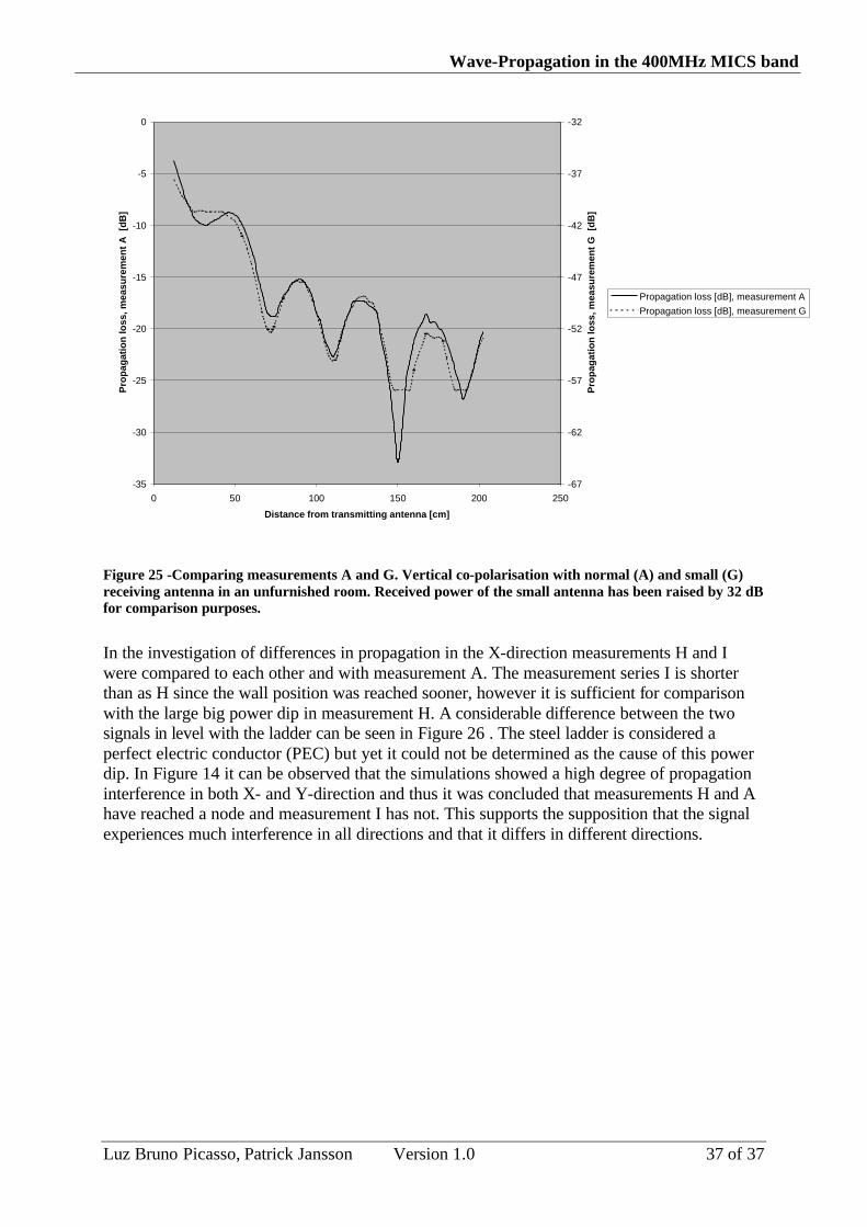
Figure 25 -Comparing measurements A and G. Vertical co-polarisation with normal (A) and small (G) receiving antenna in an unfurnished room. Received power of the small antenna has been raised by 32 dB for comparison purposes.

In the investigation of differences in propagation in the X-direction measurements H and I were compared to each other and with measurement A. The measurement series I is shorter than as H since the wall position was reached sooner, however it is sufficient for comparison with the large big power dip in measurement H. A considerable difference between the two signals in level with the ladder can be seen in Figure 26 . The steel ladder is considered a perfect electric conductor (PEC) but yet it could not be determined as the cause of this power dip. In Figure 14 it can be observed that the simulations showed a high degree of propagation interference in both X- and Y-direction and thus it was concluded that measurements H and A have reached a node and measurement I has not. This supports the supposition that the signal experiences much interference in all directions and that it differs in different directions.



-60,00

-50,00

-40,00

-30,00

-20,00

-10,00

0,00

0,0 20,0 40,0 60,0 80,0 100,0 120,0 140,0 160,0 180,0


Pro

paga

tion

loss

[dB

]

Propagation loss [dB], measurement H

Propagation loss [dB], measurement APropagation loss [dB], measurement I

Figure 26 - Comparing measurements H, I and A. H is 25° deviation from Y-axis in pos. direction and I is 25° deviation in neg. X-direction in an unfurnished room. A is along the Y-axis in an unfurnished room.

-35

-30

-25

-20

-15

-10

-5

0

0 50 100 150 200 250


Pro

pag

atio

n lo

ss [

dB

]


Propagation loss [dB], measurement J

Figure 27 - Comparing measurements A and J. Vertical co-polarisation in an unfurnished (A) and a furnished (J) room.



Differences between the room as furnished and unfurnished were noted. Comparing co- and cross-polarisation in the furnished and unfurnished room as in Figure 27 and Figure 28 the differences are clearly discernible in the cross-polarised case.

-70

-60

-50

-40

-30

-20

-10

0

0 50 100 150 200 250


Pro

pag

atio

n lo

ss [

dB

]

Propagation loss [dB], measurement BPropagation loss [dB], measurement K

Figure 28 - Comparing measurements B and K. Cross-polarisation with transmitting antenna vertically polarised and receiving antenna horizontally polarised in an unfurnished (B) and a furnished (K) room.

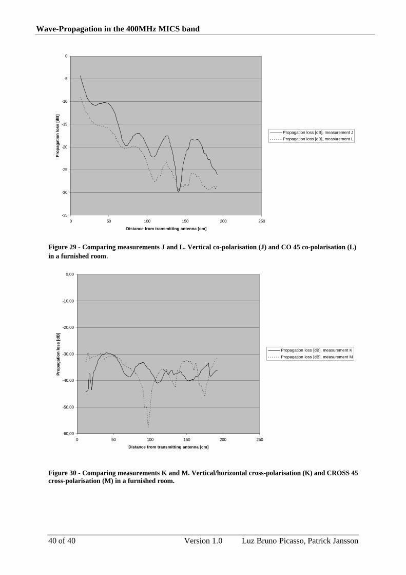
The only co- and cross-polarisations investigated thus far are vertical and horizontal; these are parallel and orthogonal to the floor, ceiling and walls of the room. Investigating beyond these specific cases measurements L and M, with the cryptic polarisation names “CO 45” and “CROSS 45”, were investigated and compared with vertical and horizontal co- and cross-polarisation. The CO 45 and CROSS 45 polarisations are detailed in chapter 5. Different co-polarisations vary as can be seen in Figure 29 and in Figure 24 previously discussed. The comparison between cross-polarisations, shown in Figure 30, highlights the lack of resemblance between the signals received.



-35

-30

-25

-20

-15

-10

-5

0

0 50 100 150 200 250


Pro

pag

atio

n lo

ss [

dB

]


Propagation loss [dB], measurement L

Figure 29 - Comparing measurements J and L. Vertical co-polarisation (J) and CO 45 co-polarisation (L) in a furnished room.

-60,00

-50,00

-40,00

-30,00

-20,00

-10,00

0,00

0 50 100 150 200 250


Pro

pag

atio

n lo

ss [

dB

]

Propagation loss [dB], measurement K

Propagation loss [dB], measurement M

Figure 30 - Comparing measurements K and M. Vertical/horizontal cross-polarisation (K) and CROSS 45 cross-polarisation (M) in a furnished room.



Comparing between the different areas of the room both furnished and unfurnished as in Figure 31 and Figure 32 a general rule of thumb can be determined. Even though the signals are fairly correlated they are attenuated. A room used for pacemaker communication should therefore preferably be sparsely furnished.

-25

-20

-15

-10

-5

0

0,0 20,0 40,0 60,0 80,0 100,0 120,0 140,0


Pro

paga

tion

loss

[dB

]


Propagation loss [dB], measurement N

Figure 31 - Comparing measurements H and N. 25° deviation from Y-axis in pos. direction in an unfurnished (H) and a furnished (N) room.

-35

-30

-25

-20

-15

-10

-5

0

0,0 20,0 40,0 60,0 80,0 100,0 120,0 140,0 160,0 180,0


Pro

paga

tion

loss

[dB

]

Propagation loss [dB], measurement I

Propagation loss [dB], measurement O

Figure 32 - Comparing measurements I and O. 25° deviation from Y-axis in neg. direction in unfurnished (I) and furnished (O) room.



Considering a person lying on the bed, an area just above the bed was measured and the power pattern of Figure 33 was given. A very noticeable area of poor reception was detected around (X, Y) = (80, 285). The root cause of this is not entirely clear, however one should bear in mind that all signals received are the result of multiple reflections. The signals received are the sum of the direct signal and all the reflections from floor, ceiling, walls and furniture in the room. This area of poor reception might be caused by interference from any or all of these signal waves, where several combine in a powerful node with the lowest measured value as -54.6 dB.

65 70 75 80 85 90 95 100

105

110

115

120

125

130

135

140

145

150

155

242,5

245

247,5250

252,5

255

257,5

260262,5

265

267,5

270

272,5275

277,5

280

282,5

285287,5

290

292,5

295

X [cm]

Y [cm]

-50--45 -45--40

-40--35 -35--30

-30--25 -25--20

-20--15 -15--10

Figure 33 - Measurement P. The area above the bed with vertical co-polarisation.



The final measurement was an NLOS (Not Line-Of-Sight) measurement, where the antenna is without visual contact. Starting inside the room, the measurements are continued through the door and on down the outside corridor. In Figure 34 the NLOS part of the measurement begins at 150 cm where the wall obstructed the line of sight. In the corridor, lockers of conducting metal created interference which can be observed at 217.5 cm. A large power dip is noticed when the measurement reaches the metallic lockers. The signal from there on does not appear to have a wavelike pattern. This is a good indicator as to how metal objects impact the signal in a negative manner. The signal weakens on reaching the wall and the antennas loose visual contact at a distance of 150 cm from the X-axis; however the reflections and the signal transmitted through the wall continue to propagate in a wavelike manner.

-60

-50

-40

-30

-20

-10

0

0 50 100 150 200 250 300 350 400 450 500

Distance, in negative direction, along X-axis from Y=127.5 cm

Pro

pag

atio

n lo

ss [

dB

]

Propagation loss [dB], measurement Q

Figure 34 - Measurement Q. Vertical co-polarisation in the corridor with a furnished room.

NLOS

Lockers



6 Results: Comparing between theory and reality

-40

-35

-30

-25

-20

-15

-10

-5

0

0 50 100 150 200



Figure 35 - Comparing measurement A and simulation SA. Transmitting antenna vertically polarised and measuring vertical polarisation in an unfurnished room.

The comparison between measurement A and simulation SA in Figure 35 are in good agreement with close to identical interference patterns. A is a noticeable difference between them was observed; the simulated series’ pattern interferes with a different phase. The cause of this is unknown but it is likely caused by values of the materials (µr, er, s E) out of alignment with the actual values. The values used in the simulations are listed in Table 2, Chapter 3.

-60

-50

-40

-30

-20

-10

0

0 50 100 150 200



Figure 36 - Comparing measurement B and simulation SB. Transmitting antenna vertically polarised and measuring horizontal polarisation in an unfurnished room.



When comparing measurement B with simulation SB in Figure 36 agreement is low except for the slopes close to and far from the antenna. The series are in agreement in so far that no value higher than -35 dB or lower than -58 dB is to be expected and both interference patterns show the same number of nodes in the interval.

-60

-50

-40

-30

-20

-10

0

0 50 100 150 200 250



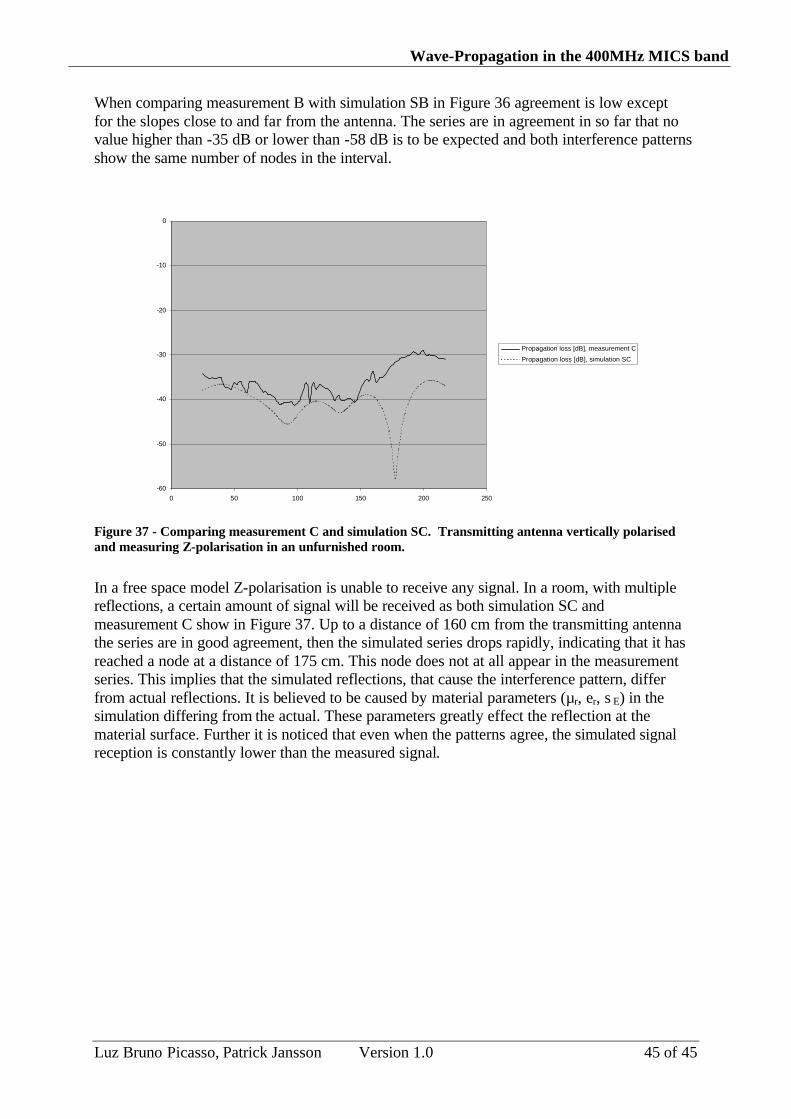
Figure 37 - Comparing measurement C and simulation SC. Transmitting antenna vertically polarised and measuring Z-polarisation in an unfurnished room.

In a free space model Z-polarisation is unable to receive any signal. In a room, with multiple reflections, a certain amount of signal will be received as both simulation SC and measurement C show in Figure 37. Up to a distance of 160 cm from the transmitting antenna the series are in good agreement, then the simulated series drops rapidly, indicating that it has reached a node at a distance of 175 cm. This node does not at all appear in the measurement series. This implies that the simulated reflections, that cause the interference pattern, differ from actual reflections. It is believed to be caused by material parameters (µr, er, s E) in the simulation differing from the actual. These parameters greatly effect the reflection at the material surface. Further it is noticed that even when the patterns agree, the simulated signal reception is constantly lower than the measured signal.



-70

-60

-50

-40

-30

-20

-10

0

0 50 100 150 200



Figure 38 - Comparing measurement J and simulation SJ. Transmitting antenna vertically polarised and measuring vertical polarisation in a furnished room.

Comparing measurement J and simulation SJ in Figure 38 shows, as in Figure 37, the simulated signal with a power dip at a distance of 180 cm which the measured signal does not have. This simulated signal reception is remarkably weaker than its measured values over all covered distances.

-60

-50

-40

-30

-20

-10

0

0 20 40 60 80 100 120 140 160



Figure 39 - Comparing measurement K and simulation SK. Transmitting antenna vertically polarised and measuring horizontal polarisation in a furnished room.



Comparing measurement K with simulation SK in Figure 39 the simulated values are, now to be anticipated, equal or lower than the measured values. This is the third simulation with a large power dip that does not occur in the measured series. The interference patterns that we detect in our simulations and measurements are caused by reflections. When they differ for simulations and measurements the waves will interfere in different manners in all three dimensions. This is the reason for the sudden power minimums in the simulated series.

In order to further study interference differences for simulations and measurements, an area over the bed was simulated and measured 66 cm above the floor. This is the height location of the chest of a patient lying on the bed. The simulation and measurement of the area are shown in Figure 40 and in Figure 41 respectively. The minimums and maximums do not occur at the exact same places when comparing the recorded power values; however the relative positioning of them is similar.

Figure 40 - Simulation of area 66 cm over the bed in a furnished room.

65 70 75 80 85 90 95 100

105

110

115

120

125

130

135

140

145

150

155

242,5

245

247,5250

252,5

255

257,5

260

262,5265

267,5

270

272,5

275

277,5280

282,5

285

287,5

290

292,5

295

X [cm]

Y [cm]

-50--45 -45--40

-40--35 -35--30

-30--25 -25--20

-20--15 -15--10

Figure 41- Measurement of area 66 cm over the bed in a furnished room.



7 Conclusions

It is essential to receive a signal co-polarised in order to receive the strongest signal. All measurements show that co-polarised signals are best received at all distances, with exception for reflections co-operating in a powerful node.

There are differences in how co-polarised waves propagate and interfere in different polarisation planes, regardless of polarisation.

Co-polarised antennas do not guarantee good transmission to all points in a room. Power measurements show that propagation loss can be as high as 55 dB at a distance 100 cm in a node, even though the antennas are co-polarised.

Furniture creates higher attenuation for wave propagation and conducting metal can also severely affect a signal. A room intended for RF communication should therefore preferably be sparsely furnished and measurements suggest that such a room should contain as few metal objects as possible.

SEMCAD gives a good picture of the interference pattern and attenuation variations in a room. It also gives reliable values of variation in signal reception. However it is based upon numerical calculations and is an approximation and not an exact indication of where in the room to find maximums or minimums. It is not clear if the differences between measurements and simulations are due to modelling approximations or measurement errors. SEMCAD requires values of µr, er, and s E that are frequency dependent and difficult to find exactly. Since very few modern walls are homogenous this leads to approximations that add to the error.



8 Discussion

In a room with interfering reflections it is not obvious where power minimums appear, however it is to be expected that several points in the room will have no signal reception due to the co-operation of several reflections. These power minimums also appear close to the transmitting antenna; at distances no further than two wavelengths the propagation loss may be as high as 55 dB. With the exception for these nodes, both measured and simulated patterns show low propagation loss in most parts of the room. To assure good signal reception anywhere in the room the use of two transmitting antennas is suggested. With two transmitting antennas the one with best link to the point of interest could be chosen and thus reduce the risk of the signal not being received. It would require further measurements and simulations to investigate the signals dependence of distance between the transmitting antennas. Alternatively a single mobile transmitting antenna may be an option.

Co-polarisation is essential to ensure good signal reception. Thus the polarisation of the implanted antenna must be known. Alternatively signals with varying polarisations could be transmitted. As in the case with two different transmitting antennas the link with best polarisation is then chosen.

An alternative antenna may very well have much higher directivity and thus might be more suitable for indoor RF communication than the dipole antennas used in this thesis. With higher directivity the reflections are weaker and do not create as much interference and powerful nodes. A disadvantage with high directivity antennas is that they become very large at frequencies as low as 400 MHz, also they must be aimed at the patient for good reception.

A hospital room is often furnished with conducting metal furniture. This should be avoided in a room intended for RF communication. It is probable that many metal objects in a room or its walls will lead to higher attenuation. Ideally a room should possibly be furnished with plastic furniture for good receiving quality of a signal.



9 References

[1] www.sjm.com

[2] www.naspe.org/ep-history/timeline/1950s/

[3] www.asmj.netfirms.com/article0903.html

[4] www.semcad.com

[5] N. Chavannes, H.U. Gerber, A. Christ, J. Fröhlich, H. Songoro, N. Kuster, “Advances in FDTD Modeling Capabilities for Enhanced Analysis of Antennas Embedded in Complex Environments”, 2001 International Conference on Electromagnetics in Advanced Applications, Torino, Italy, September 10-14, 2001

[6] K. S. Yee, “Numerical solution of initial boundary value problems involving Maxwell’s equations in isotropic media,” IEEE Triffans. Ant. Propag., vol.14, pp. 302-307, 1966

[7] Henrik Holter, “PB-FDTD” Periodic Boundary FDTD Version 3.2, February 2003

[8] Schmid & Partner Engineering AG, SEMCAD Manual Addendum V1.8, August 2003

[9] S. Y. Tang “Measurement Validation of Ray-Tracing propagation” Model on Double-Diffracted Paths, Volume 30, No3, March 2002

[10] www.asiinstr.com

[11] B. Widenberg, “Thick Frequency Selective Structures”, KFS AB, 2003

[12] Constantine A. Balanis, “Antenna Theory – analysis and design” 2nd edition, John Wiley & sons Inc, 1997

[13] David K. Cheng, “Field and wave electromagnetics” 2nd edition, Addison-Wesley Publishing Company, 1989

[14] John D. Kraus, Ronald J. Marhetka, “Antennas for all applications”, McGraw-Hill, 2002

[15] Gerald Hall, “The ARRL Handbook” 15th edition, ARRL, 1988

[16] Richard C. Johnson, Henry Jasik, “Antenna engineering handbook” 2nd edition, McGraw-Hill, 1984

[17] A.W. Rudge, K. Milne, A. D. Olver, P. Knight, “The Handbook of Antenna Design” Volumes 1 & 2, Peter Peregrinus Ltd, 1986

[18] Glenn R. Blackwell, “The Electronic Packaging Handbook”, CRC Press LLC, 2000

[19] Arai Hiroyuki, “Measurement of Mobile Antenna Systems”, Artech House, 2001



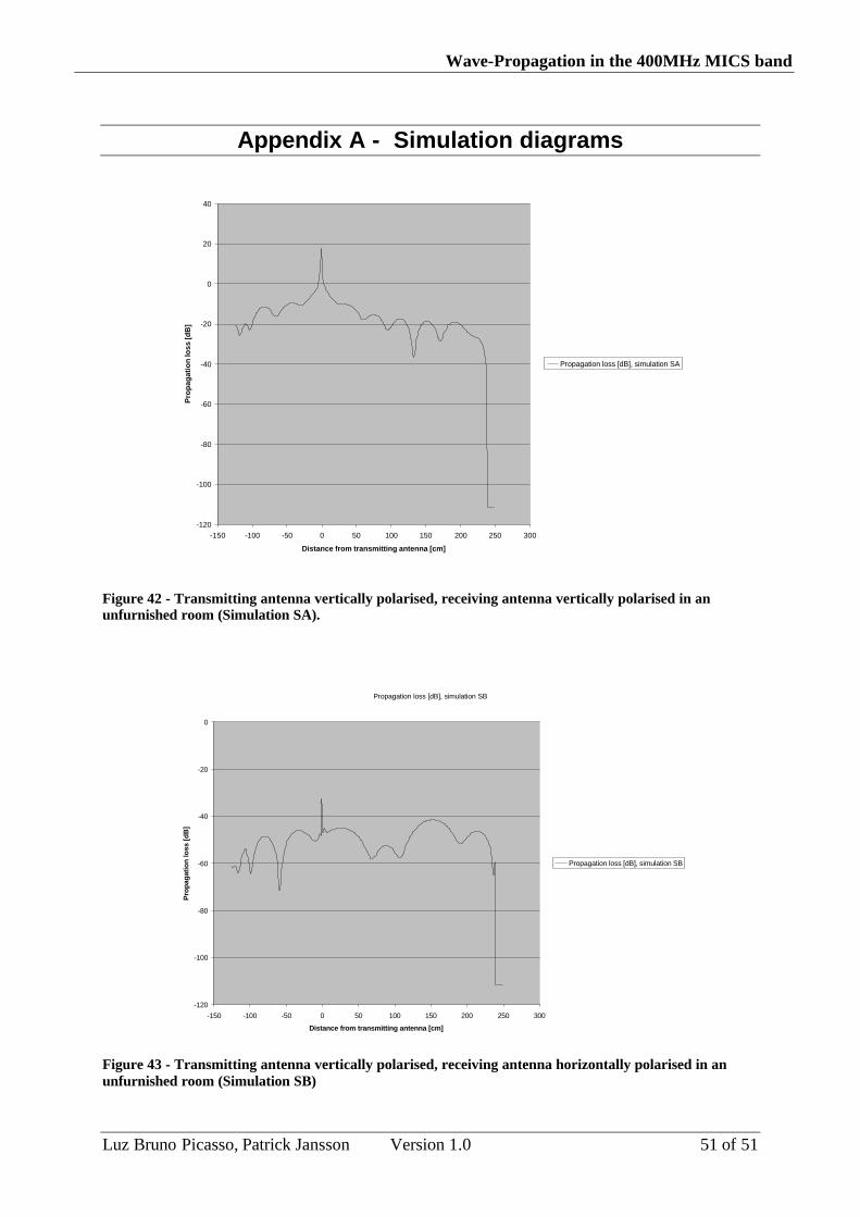
Appendix A - Simulation diagrams

-120

-100

-80

-60

-40

-20

0

20

40

-150 -100 -50 0 50 100 150 200 250 300


Pro

pag

atio

n lo

ss [d

B]


Figure 42 - Transmitting antenna vertically polarised, receiving antenna vertically polarised in an unfurnished room (Simulation SA).


-120

-100

-80

-60

-40

-20

0

-150 -100 -50 0 50 100 150 200 250 300


Pro

paga

tion

loss

[dB

]


Figure 43 - Transmitting antenna vertically polarised, receiving antenna horizontally polarised in an unfurnished room (Simulation SB)



-120

-100

-80

-60

-40

-20

0

20

40

-150 -100 -50 0 50 100 150 200 250 300


Pro

pag

atio

n lo

ss [

dB

]


Figure 44 - Transmitting antenna vertically polarised, receiving antenna Z polarised in an unfurnished room (Simulation SC).

-120

-100

-80

-60

-40

-20

0

-150 -100 -50 0 50 100 150 200 250 300


Pro

pag

atio

n lo

ss [d

B]


Figure 45 - Transmitting antenna vertically polarised, receiving antenna vertically polarised in a furnished room (Simulation SJ).



-60

-50

-40

-30

-20

-10

0

-150 -100 -50 0 50 100 150 200


Pro

paga

tion

loss

[dB

]


Figure 46 - Transmitting antenna vertically polarised, receiving antenna horizontally polarised in a furnished room (Simulation SK).



Appendix B - Antenna radiation patterns

Figure 47 - Radiation pattern for the receiving antenna

Figure 48 - Radiation pattern for the transmitting antenna



Appendix C - Measurement diagrams

-35,0000

-30,0000

-25,0000

-20,0000

-15,0000

-10,0000

-5,0000

0,0000

0,0 50,0 100,0 150,0 200,0 250,0


Pro

paga

tion

loss

[dB

]


Figure 49 - Transmitting antenna vertically polarised, receiving antenna vertically polarised in an unfurnished room (measurement A).

-70,0000

-60,0000

-50,0000

-40,0000

-30,0000

-20,0000

-10,0000

0,0000

0,0 50,0 100,0 150,0 200,0 250,0


Pro

pag

atio

n lo

ss [

dB

]


Figure 50 - Transmitting antenna vertically polarised, receiving antenna horizontally polarised in an unfurnished room (measurement B).



-45

-40

-35

-30

-25

-20

-15

-10

-5

0

0 50 100 150 200 250


Pro

pag

atio

n lo

ss [d

B]


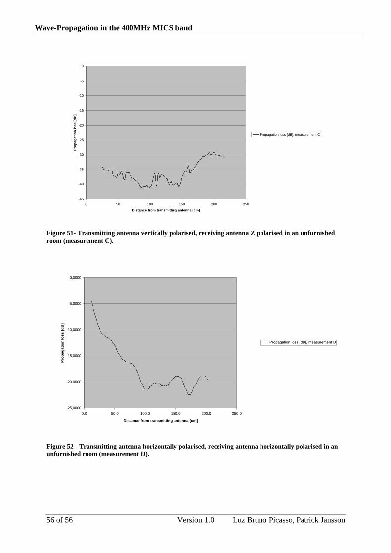
Figure 51- Transmitting antenna vertically polarised, receiving antenna Z polarised in an unfurnished room (measurement C).

-25,0000

-20,0000

-15,0000

-10,0000

-5,0000

0,0000

0,0 50,0 100,0 150,0 200,0 250,0


Pro

paga

tion

loss

[dB

]

Propagation loss [dB], measurement D

Figure 52 - Transmitting antenna horizontally polarised, receiving antenna horizontally polarised in an unfurnished room (measurement D).



-60,0000

-50,0000

-40,0000

-30,0000

-20,0000

-10,0000

0,0000

0,0 50,0 100,0 150,0 200,0 250,0


Pro

paga

tion

loss

[dB

]

Propagation loss [dB], measurement E

Figure 53 - Transmitting antenna horizontally polarised, receiving antenna vertically polarised in an unfurnished room (measurement E).

-70

-60

-50

-40

-30

-20

-10

0

0 50 100 150 200 250


Pro

pag

atio

n lo

ss [

dB

]

Propagation loss [dB], measurement F

Figure 54 - Transmitting antenna horizontally polarised, receiving antenna Z polarised in an unfurnished room (measurement F).



-60

-50

-40

-30

-20

-10

0

0 50 100 150 200 250


Pro

paga

tion

loss

, mea

sure

men

t A

[d

B]

Propagation loss [dB], measurement G

Figure 55- Transmitting antenna vertically polarised, receiving antenna vertically polarised (small antenna) in an unfurnished room (measurement G).

-60,00

-50,00

-40,00

-30,00

-20,00

-10,00

0,00

0,0 50,0 100,0 150,0 200,0 250,0


Pro

paga

tion

loss

[dB

]


Figure 56- Transmitting antenna vertically polarised, receiving antenna vertically polarised in an unfurnished room, 25 ° deviation from Y-axis in pos. X direction (measurement H).



-30,00

-25,00

-20,00

-15,00

-10,00

-5,00

0,00

0 20 40 60 80 100 120 140 160 180


Pro

paga

tion

loss

[dB

]

Propagation loss [dB], measurement I

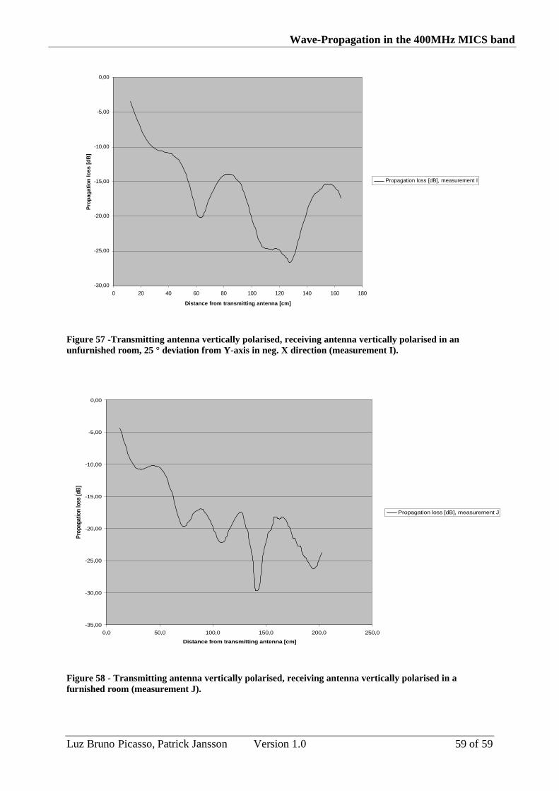
Figure 57 -Transmitting antenna vertically polarised, receiving antenna vertically polarised in an unfurnished room, 25 ° deviation from Y-axis in neg. X direction (measurement I).

-35,00

-30,00

-25,00

-20,00

-15,00

-10,00

-5,00

0,00

0,0 50,0 100,0 150,0 200,0 250,0


Prop

agat

ion

loss

[dB

]


Figure 58 - Transmitting antenna vertically polarised, receiving antenna vertically polarised in a furnished room (measurement J).



-50.00

-45.00

-40.00

-35.00

-30.00

-25.00

-20.00

-15.00

-10.00

-5.00

0.00

0 50 100 150 200 250


Pro

pag

atio

n lo

ss [

dB

]


Figure 59 - Transmitting antenna vertically polarised, receiving antenna horizontally polarised in a furnished room (measurement K).

-35.00

-30.00

-25.00

-20.00

-15.00

-10.00

-5.00

0.00

0 50 100 150 200 250


Pro

pag

atio

n lo

ss [d

B]

Propagation loss [dB], measurement L

Figure 60 - Transmitting antenna CO 45 polarised, receiving antenna CO 45 polarised in a furnished room (measurement L).



-70,00

-60,00

-50,00

-40,00

-30,00

-20,00

-10,00

0,00

0,0 50,0 100,0 150,0 200,0 250,0


Pro

pag

atio

n lo

ss [

dB

]

Propagation loss [dB], measurement M

Figure 61 - Transmitting antenna CROSS 45 polarised, receiving antenna CROSS 45 polarised in a furnished room (measurement M).

-25,00

-20,00

-15,00

-10,00

-5,00

0,00

0,0 20,0 40,0 60,0 80,0 100,0 120,0 140,0


Pro

pag

atio

n lo

ss [

dB

]

Propagation loss [dB], measurement N

Figure 62 - Transmitting antenna vertically polarised, receiving antenna vertically polarised in a furnished room, 25 ° deviation from Y-axis in pos. X direction (measurement N).



-35,00

-30,00

-25,00

-20,00

-15,00

-10,00

-5,00

0,00

0,0 20,0 40,0 60,0 80,0 100,0 120,0 140,0


Pro

pag

atio

n lo

ss [d

B]

Propagation loss [dB], measurement O

Figure 63 - Transmitting antenna vertically polarised, receiving antenna vertically polarised in a furnished room, 25 ° deviation from Y-axis in neg. X direction (measurement O).

Documents

Simulation and Measurement of Radio Wave Propagation … · DEPARTMENT OF ELECTROSCIENCE LUND INSTITUTE OF TECHNOLOGY SWEDEN Simulation and Measurement of Radio Wave Propagation in