Embed Size (px)
Citation preview

Simulation and Improvement of the Handoverprocess in IEEE 802.11p based VANETs
(Vehicle Ad-hoc NETworks)
Pablo Urmeneta
College of Electronics and Information Engineering,Tongji University
Escola Tecnica Superiord’Enginyeria de Telecomunicacio de Barcelona,
Universitat Politecnica de Catalunya
Supervised by Prof. Fuqiang Liu
Shanghai, November 2010


Abstract
This research focuses on the study of the handover process and the different simulation
environments available in order to generate valid results for the optimization of seamless
handover in VANET networks.
Handover parameter analysis has been performed and implemented in a application
developed in order to batch simulate the process of modifying the selected variables
and statistically analyzing the results in order to allow further research on the topic to
achieve valid results for VANET handover simulations in a very convenient manner.
Keywords: Handover, handoff, VANET, IEEE 802.11p, WAVE, simulation, V2I, ns-2


Contents
1 Introduction 1
2 Background 3
2.1 WAVE . . . . . . . . . . . . . . . . . . . . . . . . . . . . . . . . . . . . . 3
2.2 IEEE 802.11p . . . . . . . . . . . . . . . . . . . . . . . . . . . . . . . . . 4
2.2.1 Physical layer (PHY) . . . . . . . . . . . . . . . . . . . . . . . . . 5
2.2.2 Medium Access Control (MAC) . . . . . . . . . . . . . . . . . . . 6
2.2.3 QoS . . . . . . . . . . . . . . . . . . . . . . . . . . . . . . . . . . 6
2.3 Handover . . . . . . . . . . . . . . . . . . . . . . . . . . . . . . . . . . . 7
2.4 Handover Process . . . . . . . . . . . . . . . . . . . . . . . . . . . . . . . 7
2.4.1 Detection: Trigger . . . . . . . . . . . . . . . . . . . . . . . . . . 8
2.4.2 Discovery: Scanning . . . . . . . . . . . . . . . . . . . . . . . . . 8
2.4.3 Execution . . . . . . . . . . . . . . . . . . . . . . . . . . . . . . . 11
2.4.4 Latency . . . . . . . . . . . . . . . . . . . . . . . . . . . . . . . . 11
2.5 WAVE mode . . . . . . . . . . . . . . . . . . . . . . . . . . . . . . . . . 13
2.6 MobileIP . . . . . . . . . . . . . . . . . . . . . . . . . . . . . . . . . . . . 14
2.7 Cross-Layer communication . . . . . . . . . . . . . . . . . . . . . . . . . 15
2.8 Media Independent Handover . . . . . . . . . . . . . . . . . . . . . . . . 15
i

3 Simulation System 17
3.1 Mobility Simulators . . . . . . . . . . . . . . . . . . . . . . . . . . . . . . 18
3.1.1 BonnMotion . . . . . . . . . . . . . . . . . . . . . . . . . . . . . . 19
3.1.2 CanuMobiSim . . . . . . . . . . . . . . . . . . . . . . . . . . . . . 19
3.1.3 SUMO . . . . . . . . . . . . . . . . . . . . . . . . . . . . . . . . . 20
3.1.4 Commercial Solutions . . . . . . . . . . . . . . . . . . . . . . . . 20
3.2 Network Simulators . . . . . . . . . . . . . . . . . . . . . . . . . . . . . . 21
3.2.1 ns-2 . . . . . . . . . . . . . . . . . . . . . . . . . . . . . . . . . . 21
3.2.2 ns-3 . . . . . . . . . . . . . . . . . . . . . . . . . . . . . . . . . . 24
3.3 Integrated Mobility and Network Simulators . . . . . . . . . . . . . . . . 25
3.3.1 GloMoSim . . . . . . . . . . . . . . . . . . . . . . . . . . . . . . . 25
3.3.2 NCTUns . . . . . . . . . . . . . . . . . . . . . . . . . . . . . . . . 25
3.3.3 OMNeT++ . . . . . . . . . . . . . . . . . . . . . . . . . . . . . . 26
3.3.4 Commercial Solutions . . . . . . . . . . . . . . . . . . . . . . . . 27
3.4 Federated solutions . . . . . . . . . . . . . . . . . . . . . . . . . . . . . . 28
3.4.1 SUMO/ns-2 . . . . . . . . . . . . . . . . . . . . . . . . . . . . . . 28
3.4.2 SUMO/QualNet . . . . . . . . . . . . . . . . . . . . . . . . . . . 29
3.5 Selection . . . . . . . . . . . . . . . . . . . . . . . . . . . . . . . . . . . . 29
3.5.1 Network Simulator . . . . . . . . . . . . . . . . . . . . . . . . . . 29
3.5.2 Mobility Simulator . . . . . . . . . . . . . . . . . . . . . . . . . . 31
4 Handover Optimization 33
4.1 Parameter Optimization . . . . . . . . . . . . . . . . . . . . . . . . . . . 33
4.1.1 Procedure . . . . . . . . . . . . . . . . . . . . . . . . . . . . . . . 33
4.1.2 Simulation Scenario . . . . . . . . . . . . . . . . . . . . . . . . . . 34
4.1.3 Simulation Parameters . . . . . . . . . . . . . . . . . . . . . . . . 39
4.2 System Configuration . . . . . . . . . . . . . . . . . . . . . . . . . . . . . 43
4.2.1 ns-2 Simulation Scripts . . . . . . . . . . . . . . . . . . . . . . . . 43
4.2.2 Batched simulation . . . . . . . . . . . . . . . . . . . . . . . . . . 44
ii
4.2.3 Performance evaluation . . . . . . . . . . . . . . . . . . . . . . . . 46
4.3 Strategies for further optimization . . . . . . . . . . . . . . . . . . . . . . 47
4.3.1 Trigger optimization . . . . . . . . . . . . . . . . . . . . . . . . . 47
4.3.2 Choice of RSU for the handover . . . . . . . . . . . . . . . . . . 47
4.3.3 Implementation of MIHand Cross-Layer Communication . . . . . . . . . . . . . . . . . . 48
4.3.4 Reducing the Discovery Latency . . . . . . . . . . . . . . . . . . . 48
4.3.5 Using mobility/environment parameters . . . . . . . . . . . . . . 49
5 Conclusions 51
A Installation 53
A.1 ns-2 . . . . . . . . . . . . . . . . . . . . . . . . . . . . . . . . . . . . . . 53
A.2 NOAH - No Ad-Hoc Routing . . . . . . . . . . . . . . . . . . . . . . . . 53
B ns-2 Simulation Scripts 57
B.1 Without Mobile IP . . . . . . . . . . . . . . . . . . . . . . . . . . . . . . 57
B.2 With Mobile IP . . . . . . . . . . . . . . . . . . . . . . . . . . . . . . . . 63
C Batched Simulations and Analysis 69
C.1 Bash Shell Script for Batched Simulations . . . . . . . . . . . . . . . . . 69
C.1.1 Considerations . . . . . . . . . . . . . . . . . . . . . . . . . . . . 69
C.1.2 Interface . . . . . . . . . . . . . . . . . . . . . . . . . . . . . . . . 71
C.1.3 Output . . . . . . . . . . . . . . . . . . . . . . . . . . . . . . . . . 72
C.1.4 Expanding the framework . . . . . . . . . . . . . . . . . . . . . . 73
C.1.5 Code . . . . . . . . . . . . . . . . . . . . . . . . . . . . . . . . . . 74
C.2 AWK scripts for analysis of batched simulations . . . . . . . . . . . . . . 84
C.2.1 Code . . . . . . . . . . . . . . . . . . . . . . . . . . . . . . . . . . 84
Bibliography 91
List of Figures 95
List of Tables 97
iii


Chapter 1
Introduction
Vehicular Ad-hoc NETworks are a subset of the Mobile Ad-hoc NETworks —MANETs—
which provide wireless communication capabilities between devices in a certain range.
In a VANET environment this devices are either stations (STAs) installed in vehicles
as on board units (OBUs) or access points (APs) strategically located in fixed points
along the road, and hence usually referred to as road side units (RSUs).
Vehicular Ad-Hoc Networks have been a very active research topic in the last years
due to the very positive impact of their implementation in road safety.
For security communications, which require short message exchange, there is no
need to implement a seamless handover scheme, as it would imply a rather significant
signaling overhead, delaying the communications to a point where the security message
may be invalid or the communications to be enabled when the vehicle is close to leaving
the service area.
However, security communications are not the only goal of VANETs: there are a
number of applications that require continuous communications during periods of time
that exceed the span available when the mobile node (MN) is traveling through the
service area of a given RSU, such as voice over IP (VoIP), video streaming, etc. For
that reason the possibility of performing seamless handover between RSUs should be
available to support this services which, even though not as a priority, are expected to
be used over VANETs.
The aim is the study of the available simulation environments for VANETs, the
modeling of the simulation environment and the analysis of the results in order to
optimize the IEEE 802.11p protocol parameters in order to provide fast and reliable
seamless handover —when the system is not working on what will be later defined as
WAVE mode— for the mobile devices while moving between the transmission ranges of
1

different infrastructure nodes. Optimization strategies not based on parameter choice
have been presented for further research.
The research will present a system that has been developed in order to allow a
researcher to setup the desired handover parameters for automated simulation, obtain-
ing relevant results in a convenient manner with an almost inexistent learning curve.
This system also includes analysis capabilities for the simulation results, considerably
enhancing the research workflow.
This thesis has been developed in the framework of the BMW Lab. in Tongji Uni-
versity, where a major research is the development and implementation of VANETs.
This research is intended to improve the performance of the current research in terms
of seamless handover.
This report is organized as follows: Chapter 2 focuses on the specifics of VANETs,
with special interest on the handover process. Chapter 3 summarizes the study per-
formed in order to select the most suitable simulation system. Chapter 4 presents the
study of the IEEE 802.11p parameters, focusing on those that will have a significant im-
pact on the handover performance, the specifics of the framework developed to perform
the desired simulations in a batched manner and the optimization strategies which are
not parameter-based. Chapter 5 summarizes the achievements of the research and pro-
poses further research on seamless handover to extend the reach of the current research.
2
Chapter 2
Background
2.1 WAVE
WAVE, namely Wireless Access in the Vehicular Environment, defines a mode of oper-
ation for IEEE 802.11p devices in those situations where the properties of the physical
layer are rapidly changing and where the duration of the communication exchange is
remarkably short. Rapidly changing environment and the nature of the information ex-
changed in vehicular networks requires a system which can allow the nodes to actually
complete the data transmission in a much shorter period of time than that required by
other wireless protocols to authenticate and associate to join either a infrastructure or
an ad-hoc network.
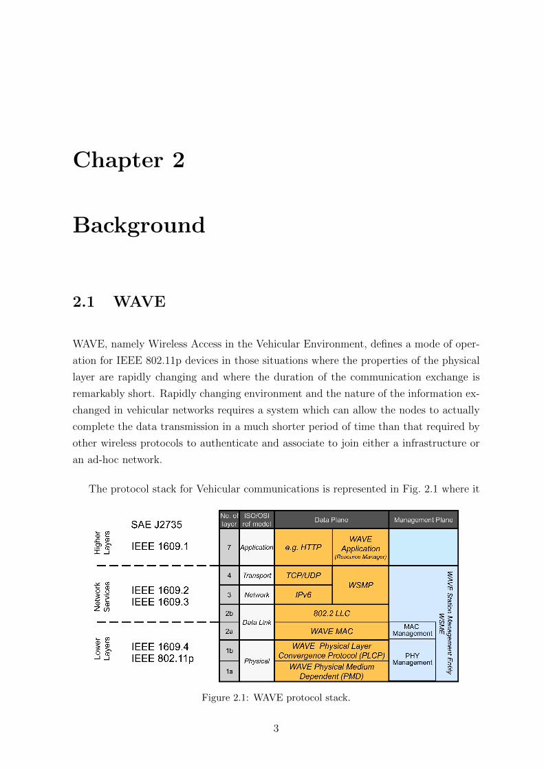
The protocol stack for Vehicular communications is represented in Fig. 2.1 where it
Figure 2.1: WAVE protocol stack.
3

can be observed that the family of standards P1609.x provide an implementation of the
higher OSI levels while it relies on the IEEE 802.11p protocol to provide the lower levels
implementation.
Considering the communication requirements, WAVE defines an implementation of
IEEE 802.11p for devices which is able to enable communication by defining the mini-
mum set of parameters that will ensure interoperability between wireless devices which
require to communicate in the previously mentioned conditions, which is called the
WAVE mode (view section 2.5).
2.2 IEEE 802.11p
The protocol IEEE 802.11p is an amendment of the IEEE 802.11-2007 protocol for wire-
less networks which focuses on the improvement of the performance of the CSMA/CA
networks in highly mobile ad-hoc networks.
This protocol is still in draft status pending for approval by the IEEE organization.
It is the proposed standard of the DSRC —Direct Short Range Communications— in
the vehicular environment by the IEEE organization, and considering the global success
of the IEEE 802.11 standard, the derived IEEE 802.11p version has the potential of
becoming a single global standard for the communications in Intelligent Transportation
Systems (ITS)[1].
The design requirements of the standard are the following:
• Longer ranges of operation: target of aprox. 1000m.
• High relative speed between nodes: up to 500km/h. Doppler effect has a high
impact in the communication.
• Extreme multi-path environment.
• Operation of multiple potentially overlapping ad-hoc networks.
• High quality of service (QoS).
• Support for vehicular-oriented applications such as safety message broadcasting.
The implementation of IEEE 802.11p is easily understandable considering the other
amendments of the IEEE 802.11 protocol. At this point the aspects 802.11p has in
common with other of the IEEE 802.11 family protocols will be explained, which provide
a very comprehensive way to understand the protocol:
4

• The physical layer of the IEEE 802.11p protocol is based on the one of IEEE
802.11a: similar orthogonal frequency-division multiplexing (OFDM) based mod-
ulation is used and the frequency allocation at the 5GHz band.
• Medium Access Control (MAC) is that of IEEE 802.11: Carrier Sense Multiple
Access with Collision Avoidance (CSMA/CA).
• For Quality of Service (QoS) the implementation has been adapted from the pro-
tocol IEEE 802.11e: Four Access Categories (ACs). Each AC has its own trans-
mission queue with built-in priorities.
IEEE 802.11p does not only implement features from other IEEE 802.11 protocols,
as the design requirements are unique in the protocol family. The main qualities which
differentiate this protocol, required to meet the essential requirements of high speed and
short communication intervals using exclusively the available resources, are:
• Dedicated frequency band (5.850 to 5.925 GHz).
• The channel bandwidth differs: 10MHz per channel instead of 20MHz. This im-
plies the data rate is also halved, alongside the symbol and guard periods being
doubled.
• Short Interframe Space (SIFS) times increased in order to prevent long-range
issues.
• Polling-based Collision-Free Phase (CFP), present in other versions of IEEE 802.11,
is not part of the 11p amendment as it would not be effective in a extremely dy-
namic environment. Therefore, no guarantee of timely delivered real-time data
packets can be offered.
• Introduction of the WAVE operation mode: allows fast communication setup when
certain conditions are met (see section 2.5).
2.2.1 Physical layer (PHY)
The Federal Communication Commission (FCC) of the U.S. approved 75 MHz band-
width at 5.850-5.925 GHz frequency band. The available band is divided into seven
10 MHz bandwidth channels (CHs 172 to 184), of which CH 178 is designated as the
Control Channel (CCH). CCH usage is limited to broadcast of safety-related data and
transmission of control and management messages. The remaining channels are Service
Channels (SCHs) available for non-safety related data transmission, including general
5
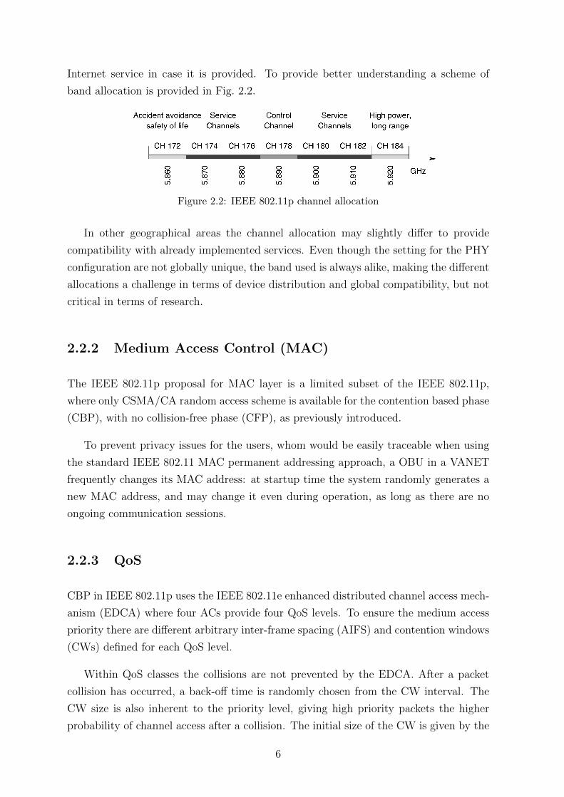
Internet service in case it is provided. To provide better understanding a scheme of
band allocation is provided in Fig. 2.2.
Figure 2.2: IEEE 802.11p channel allocation
In other geographical areas the channel allocation may slightly differ to provide
compatibility with already implemented services. Even though the setting for the PHY
configuration are not globally unique, the band used is always alike, making the different
allocations a challenge in terms of device distribution and global compatibility, but not
critical in terms of research.
2.2.2 Medium Access Control (MAC)
The IEEE 802.11p proposal for MAC layer is a limited subset of the IEEE 802.11p,
where only CSMA/CA random access scheme is available for the contention based phase
(CBP), with no collision-free phase (CFP), as previously introduced.
To prevent privacy issues for the users, whom would be easily traceable when using
the standard IEEE 802.11 MAC permanent addressing approach, a OBU in a VANET
frequently changes its MAC address: at startup time the system randomly generates a
new MAC address, and may change it even during operation, as long as there are no
ongoing communication sessions.
2.2.3 QoS
CBP in IEEE 802.11p uses the IEEE 802.11e enhanced distributed channel access mech-
anism (EDCA) where four ACs provide four QoS levels. To ensure the medium access
priority there are different arbitrary inter-frame spacing (AIFS) and contention windows
(CWs) defined for each QoS level.
Within QoS classes the collisions are not prevented by the EDCA. After a packet
collision has occurred, a back-off time is randomly chosen from the CW interval. The
CW size is also inherent to the priority level, giving high priority packets the higher
probability of channel access after a collision. The initial size of the CW is given by the
6

factor CWmin. Each time a transmission attempt fails, the CW size is doubled until
reaching the size given by the parameter CWmax. Table 2.1 summarizes the EDCA
parameters for 802.11p, where 1 denotes the highest priority level and 4 the lowest.
QoS Class CWmin CWmax AIFSN AIFSN
4 15 1023 9 149
3 15 1023 6 110
2 7 15 3 71
1 3 7 2 58
Table 2.1: EDCA parameters depending on QoS level[2]. CW in slots and AIFS in µs.
It has to be reminded that even though this priority system increases the probability
of certain packets to access the wireless channel, there are no guarantees that this will
happen before a predefined deadline, due to the absence of CFP.
2.3 Handover
Handover, also called handoff, is the process required to transfer the network connec-
tivity of a mobile node from one infrastructure node to another. In this report the
mobile node is usually an OBU and the infrastructure nodes are RSUs. Provided that
transferring only the physical and medium access control layers is not always enough
to keep the communication, in addition to the lower layers it may also be needed to
transfer information regarding higher levels of the OSI model, such as context or state
information regarding the mobile node.
2.4 Handover Process
The handover process involves at least two infrastructure nodes and one client node.
The client node is required to be attached to one of the infrastructure nodes. When the
situation evolves there will be a point where the connectivity parameters of the link will
decrease, usually due to the distance between the infrastructure and the client nodes.
In the instant the connection quality degrades to a pre-defined threshold the handover
process will start. This process can be divided into steps in a variety of ways. In this
paper and for the convenience of the classification in the following optimization we will
use the division presented by Velayos and Harrlsson at [3], where handover consists of
the next phases:
7
• Detection
• Discovery
• Execution
As will be described in detail in the following sections, the detection phase is the re-
alization of the need to handover. The search phase covers from the acquisition of
the information of all the available RSUs to the choice of the best candidate for the
handover. Finally, the handover is completed during the execution phase.
2.4.1 Detection: Trigger
Handover starts once one or more conditions occur: these conditions are called triggers,
and define the starting instant for the whole handover process. Triggers indicate the
system which is the appropriate moment to proceed to handover. Hence, this phase
has an impact in the outcome of the whole process, as the optimization of the moment
to trigger the handover may lead to a reduction of the handover latency and also the
reduction of data loss, mainly when there are overlapping networks.
There can be a variety of triggers, according to the parameters evaluated to indicate
the handover start. Traditionally these triggers are related to the network parameters
of the link, namely signal strength, bit error rate (BET), quality of service, etc. but in
the VANET environment there is the chance to go one step further and use mobility to
predict the evolution of the connectivity, thus being able to introduce parameters such
as possible paths (the vehicle’s movement is clearly restricted to a reduced number of
predefined roads), relative speed, destination (very interesting regarding public transport
vehicles, which can also be enabled as infrastructure nodes), etc. allowing the choice of
an optimized handover starting time according to the environment through the use of
context-aware triggers.
2.4.2 Discovery: Scanning
Once it has been decided that there is the need to perform a handover, the client node
will proceed to search for new candidates to attach to, checking the available medium
sequentially in order to find an AP operating as infrastructure node. When the scanning
is over the STA will sort all the processed responses and, according to the parameters
established, will decide which will be the best candidate to perform the handover.
There are two scanning procedures, namely active and passive:
8
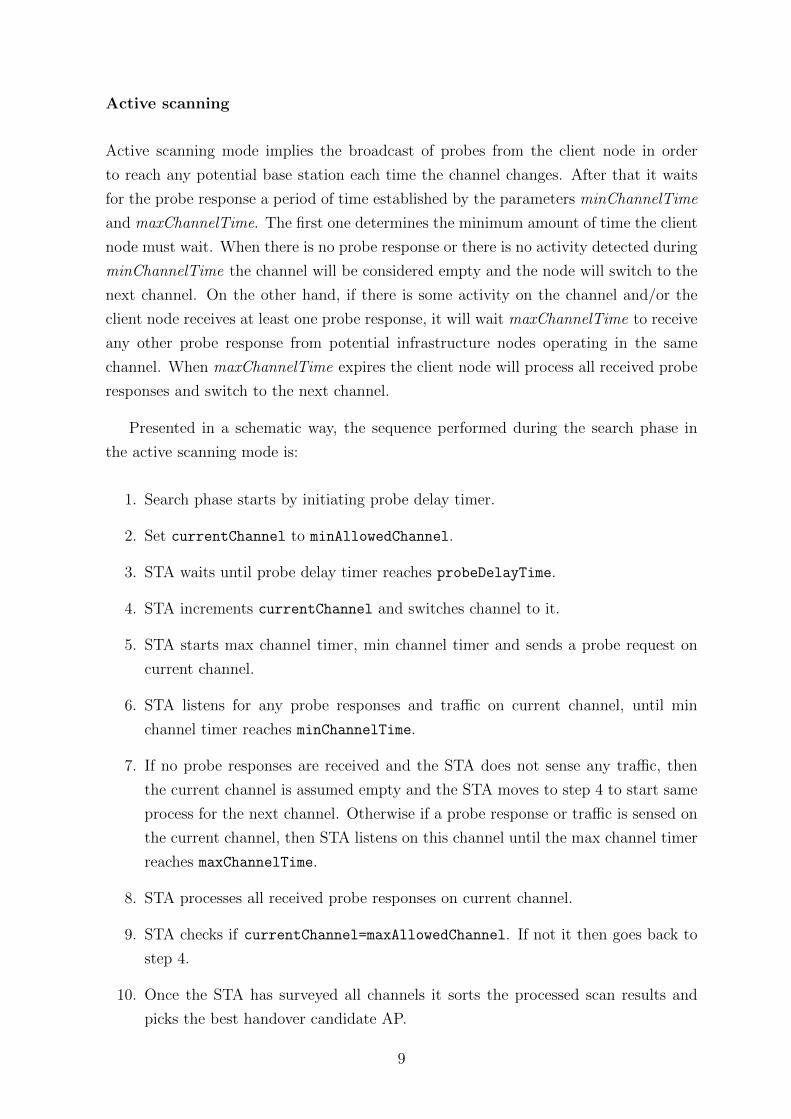
Active scanning
Active scanning mode implies the broadcast of probes from the client node in order
to reach any potential base station each time the channel changes. After that it waits
for the probe response a period of time established by the parameters minChannelTime
and maxChannelTime. The first one determines the minimum amount of time the client
node must wait. When there is no probe response or there is no activity detected during
minChannelTime the channel will be considered empty and the node will switch to the
next channel. On the other hand, if there is some activity on the channel and/or the
client node receives at least one probe response, it will wait maxChannelTime to receive
any other probe response from potential infrastructure nodes operating in the same
channel. When maxChannelTime expires the client node will process all received probe
responses and switch to the next channel.
Presented in a schematic way, the sequence performed during the search phase in
the active scanning mode is:
1. Search phase starts by initiating probe delay timer.
2. Set currentChannel to minAllowedChannel.
3. STA waits until probe delay timer reaches probeDelayTime.
4. STA increments currentChannel and switches channel to it.
5. STA starts max channel timer, min channel timer and sends a probe request on
current channel.
6. STA listens for any probe responses and traffic on current channel, until min
channel timer reaches minChannelTime.
7. If no probe responses are received and the STA does not sense any traffic, then
the current channel is assumed empty and the STA moves to step 4 to start same
process for the next channel. Otherwise if a probe response or traffic is sensed on
the current channel, then STA listens on this channel until the max channel timer
reaches maxChannelTime.
8. STA processes all received probe responses on current channel.
9. STA checks if currentChannel=maxAllowedChannel. If not it then goes back to
step 4.
10. Once the STA has surveyed all channels it sorts the processed scan results and
picks the best handover candidate AP.
9
11. Search phase ends.
In multi-channel systems, active scanning may decrease the latency when compared
to the passive scanning. On the other hand it requires more bandwidth and energy.
Passive scanning
In this scanning mode, as opposed to active scanning mode, the STA switches from one
channel to the next and waits a previously established time ChannelTime to receive
signal from any node which may be operating in that channel.
The procedure for passive scanning is akin to the one for active scanning, but ac-
cording to the algorithm presented there are a few modifications in the following steps:
5. STA switches channel to currentChannel, starts channel timer.
6. STA listens for any traffic until channel timer reaches channelTime.
7. If the STA does not sense any traffic, then the current channel is assumed empty
and the STA moves to step 9. If on the other hand traffic has been sensed, STA
moves to step 8.
The advantage of passive scanning is the low power and bandwidth requirements,
but it may increase the latency of the discovery phase for low activity channels as it
does not proactively generate traffic. As the possibility that the switch to the channel
occurred just after the beacon exists, the listening time has to be at least the same
as the beaconing interval of the protocol to prevent considering a channel empty when
there are nodes operating in it.
10

2.4.3 Execution
Figure 2.3: Handover process
The handover execution takes
place when the need to handover
has been determined, the channel
has been surveyed and a candi-
date for the handover is selected.
At that point, and as shown in
fig. 2.3, the client node will try
to connect to the infrastructure
node by sending an authentica-
tion message.
Once the response to it from
the infrastructure node, it would
send a re-association frame, wait
for the response and after that fi-
nal step the communication be-
comes possible for the mobile
node. In some situations where
there is a need to maintain previous sessions, the new AP will send the re-association
response after exchanging context information with the old AP in order to keep the
same sessions open, making seamless handover possible for higher stack levels of the
protocol architecture.
2.4.4 Latency
As there is no standard procedure to measure the handover latency in the literature,
and taking into account the previous definition of the handover process, we will consider
two different concepts: the strict handover latency and the complete handover latency.
The strict handover latency is considered the contribution of the search phase and
the handover execution. The contribution of each of them is:
THandover Strict = TScan + TExecution
The search time (TScan) starts at the moment the mobile node starts its probe delay
timer to the instant that the candidate for the handover has been determined. The
11

execution phase follows and is the responsible for the rest of the handover strict latency:
TExecution.
TScan for passive scan is TScan passive = Nchannels × ChannelT ime, while for active
scan is bounded as in the equation:
Nchannels ×MinChannelT ime ≤ TScan active ≤ Nchannels ×MaxChannelT ime
There are some considerations regarding THandover Strict: The detection time and the
impact of level 3 or higher layers of the architecture are not taken into account. That is
the reason why the concept of strict handover is not enough to achieve the optimization
of the whole handover process.
The complete handover latency not only consists of the strict latency but it takes
into account those aspects which will certainly influence the handover process, either
by modifying its decisions, affecting its latency or altering the chances to be successful.
Recalling the previously defined handover process steps, namely detection, discovery
and execution, the complete handover latency is:
THandover Complete = TDetection + TDiscovery + TExecution
= TDetection + THandover Strict
At the same time, it is crucial to differentiate the values of the downstream latency
from the upstream and bidirectional latency. Due to the use of buffers, which may mask
the real results of the simulation in terms of latency, the handover latency has to be
considered as follows:
Downstream latency consists of the time between the reception of the last data
packet sent or routed from the old RSU until the mobile node is able to receive another
data packet sent by or through the new infrastructure node. This time is the key for
the avoidance of accidents as it is the time the mobile node is not able to be directly
informed by any RSU.
Upstream latency comprises the time between the last successfully sent packet from
the OBU until there is another successfully delivered packet to the same destination
being routed through the new RSU.
According to the previous definitions, bidirectional latency is consequently the max-
imum value between downstream and upstream latency.
12

2.5 WAVE mode
IEEE 802.11 MAC operations described above imply a considerable latency. This makes
the standard handover approach unsuitable for safety communications, which require
the fastest possible data exchange and therefore cannot afford the delay introduced by
scanning the medium and handshake to establish the communication.
In order to solve this the “WAVE mode” was developed: all the radio channels
are set up in the same channel and have the same configuration for that subset of
parameters —such as the basic service set identifier (BSSID)— required to enable instant
communication. This allows a station (STA) in WAVE mode to transmit and receive
data frames with the predefined BSSID value regardless of whether the node belongs
or not to a basic service set (BSS), called in this mode a WAVE BSS (WBSS). This
procedure allows two nodes to instantly start a communication by only setting up the
predefined channel and the wildcard BSSID.
A WAVE station uses a on demand beacon to advertise a WBSS, which contains all
the needed information for receiver stations to notice the services offered in the WBSS
as well as the information needed to configure itself to become a member of the WBSS.
Accordingly, a STA can decide whether to join and complete the process of becoming
part of a WBSS by only receiving a single WAVE advertisement beacon with no further
interaction with the advertiser.
This approach provides a low overhead WBSS setup by removing all association and
authentication phases. However, it requires complementary mechanisms at upper layers,
the already introduced P1609.x protocol family among others, to manage the WBSS as
well as to provide security, features required to prevent deceptive information, potential
attacks within the WBSS such as denial of service, etc.
The lack of an association phase when a vehicle enters the WBSS prevents the
MAC address of the OBU to be passed to the advertiser, further enhancing privacy
preventing the RSU to identify a WBSS member. On the other hand, the absence of an
association and de-association process prevents any RSU to know whether a OBU has
left its transmission range.
It has to be noted that for non-safety communications that require long periods of
connectivity —such as VoIP, audio or video streaming. . . — seamless handover capabil-
ities when moving between RSUs transmission ranges are still required.
13

2.6 MobileIP
Mobile IP (MIP) allows handover to maintain existing network connections when moving
to a new subnet. The basic handover procedures involve two components, the already
explained handover —operating at Level2— and L3 handover —operating at Level3—.
L2 handover supports for roaming at the link layer while L3 handover occurs at the
network layer level. The MIPv4 handover takes place after the L2 handover and its
procedure is depicted in Figure 2.4, where CoA refers to Care of Address: a temporary
IP address to allow a home agent to forward messages to the mobile node.
Figure 2.4: Mobile IPv4 Handover [4].
MIP handover will contribute to the handover latency with TMIP = Tdetect + TCoA +
Tredirect, which in case the system is using MIP must be considered for the complete
handover latency, as there will not be a full connectivity with the Home Agent (HA)
until that procedure has been concluded:
T ′Handover Complete = THandover Complete + TMIP
= THandover Complete + Tdetect + TCoA + Tredirect
14

2.7 Cross-Layer communication
The structure of the conventional protocols is inflexible, requiring layers to communicate
in a strict manner and exclusively between adjacent layers with a restricted number of
methods available, preventing the system to adapt to dynamic conditions inherent to
VANETs. This results in poorly efficient use of resources, mainly bandwidth and energy,
critical in wireless environments.
To minimize the effect of the communication architecture a new approach to protocol
implementation is needed, characterized by cross-layer design and adaptation.
In general, cross-layer design involves five key layers in the protocol stack: application
layer, transport layer, network layer, medium access layer, and physical layer. QoS,
Security, Mobility and Wireless Link Adaptation should be carefully examined in a
cross-section view of the protocol stack.
The implementation of cross-layer communication in the design of the VANET ar-
chitecture holds a greater potential[5] as it would allow higher levels to be informed
at critical instants, as when the link is going down, and therefore optimize the data
transmission to minimize the impact of those events in the handover, thus maximizing
the chances of success.
2.8 Media Independent Handover
Media Independent Handover (MIH), also referred to as Vertical Handover, as opposed
to the already introduced handover which is also denominated Horizontal Handover, is
a system which allows the handover process between networks whether or not they are
of different media types, increasing the possibilities in situations such as when one of
the network is unavailable.
The IEEE has developed the protocol IEEE 802.21[6] to provide MIH where han-
dover is not otherwise defined, making possible for mobile devices to perform seamless
handover where the involved networks support it. MIH can be applied between IEEE
802 protocols regardless of the media type, as between wired —IEEE 802.3 (LAN)— and
wireless protocols —IEEE 802.11 (WLAN), IEEE 802.16 (WiMAX)—, or between these
and non IEEE 802 networks such as cellular —UMTS (3G)— or digital broadcasting
—Digital Video Broadvasting (DVB)— networks.
This topic has already been researched by the BMW Lab. at Tongji University —
National High-Tech 863 project— and will not be addressed in this research.
15

Chapter 3
Simulation System
There are three main techniques to analyze the behavior of a system: Analytical Mod-
eling, Computer Simulations and Real Time Physical Measurements. Analytical Mod-
eling may be impossible for complex systems such as the one of this research and Real
Time Physical Measurements would require a very long time to be performed and a
considerable investment in equipment and resources. Computer Simulation is the only
reasonable approach to the quantitative analysis of both traffic and computer networks
for this research.
Computer Simulation may be based on the Discrete Event Simulation (DES) ap-
proach, which is based on a event scheduler and only calculates the impact of those
events, or Continuous Simulations, which simulates the whole system for all the instants
simulated. For example, the simulation of one car moving at a certain speed along a
road without obstacles can be simulated continuously or either configure a event cor-
responding to the next instant that the vehicle has to modify its movement, saving a
considerable amount of simulation time and computer resources. Consequently, when
possible computer based simulators use the DES approach.
Diverse simulation environments have been tested in order to recommend the best
option for the optimization of the handover in 802.11p environments. In this chapter
they will be presented and analyzed alongside their advantages and disadvantages.
Even though the simulators share a main set of features, each one has its own
distinctive characteristics, which will be the parameters which will determine the best
option for our simulation requirements.
The node mobility simulation, very important for realistic VANET simulation results,
can be either integrated in the same software suite as the network simulator or, on the
17

other hand, be based on a federation of different software who can interact properly by
means of trace translation, etc.
3.1 Mobility Simulators
Mobility simulators classification ranges from sub-microscopic to macroscopic depending
on the level of detail of the simulation. This is reflected on the smallest entity considered
by the simulator. Macroscopic simulators consider the whole traffic flow as the basic
entity.
On the other hand, microscopic simulation considers the vehicle the smallest sim-
ulation unit. There are simulators which are in-between macroscopic and microscopic,
referred as mesoscopic. The latter consider individual vehicles moving between queues,
which are the main simulated entity.
There are also sub-microscopic simulators which consider not only each vehicle, but
also the components of them, as the engine or the gear-box, and their parameters. The
different granularities are represented in Fig. 3.1.
Figure 3.1: Mobility simulator categories. From left to right: macroscopic, microscopic, sub-microscopic (within the circle: mesoscopic).
For VANET simulations, where every individual vehicle will be considered a node
and the simulation of the vehicle components and their status are not relevant, the most
adequate approach to mobility simulation is microscopic. It provides enough resolution
of the system as to provide realistic traces, but without the overload of simulating
sub-microscopic details which would not provide relevant information for this research.
18

3.1.1 BonnMotion
Developed by the University of Bonn, is a probably the most popular mobility scenario
generator and analysis tool among MANET (Mobile Ad-hoc NETworks) researchers.
It implements diverse mobility models which can be configured according to the sce-
nario needs. However, the only model directly related to VANET simulations is the
Manhattan Grid. The scenarios can be exported for the network simulators ns-2, Glo-
MoSim/QualNet, and MiXiM, network simulation software that will be introduced in
the following section.
BonnMotion is well documented and its installation process proves to be simple.
Being a java-based command-line software it is available for any operating system.
3.1.2 CanuMobiSim
The Mobility Simulation Environment developed by the CANU (Communication in Ad-
hoc Networks for Ubiquitous Computing) Research Group of the University of Stuttgart
is a flexible framework for mobility modeling.
The framework is focused on user mobility models, as it integrates spatial environ-
ment model, user trip sequences, and user movement dynamics. It includes parsers
for geographic data in various formats, and in order to simulate movement dynamics, it
provides implementations of several models from physics and vehicular dynamics. Addi-
tionally, the framework contains several random mobility models, like Brownian Motion
or Random Way-point Movement.
It is available as a stand-alone java application, and consequently is possible to
execute it in virtually any operating system.
VanetMobiSim
VanetMobiSim is a CanuMobiSim extension developed by Institut Eurecom and Po-
litecnico di Torino which focuses on vehicular mobility with realistic automotive motion
models at both macroscopic and microscopic levels.
VanetMobiSim can import TIGER maps or randomly generate them using Voronoi
tessellation. Also, it adds support for multi-lane roads, separate directional flows, dif-
ferentiated speed constraints and traffic signs at intersections.
19

Mobility models which were not available in CamuMobiSim have been integrated,
providing realistic car-to-car and car-to-infrastructure interaction. According to these
models, vehicles regulate their speed depending on nearby cars, overtake each other and
act according to the traffic condition.
3.1.3 SUMO
Simulation of Urban MObility [7][8] is a microscopic open source traffic simulator based
on command-line which incorporates realistic traffic simulation algorithms, with the
possibility to have different types of vehicles, different networks —from generated grid,
spider-web or random artificial roads to imported VISUM, Tiger, OSM, etc. models—,
and has a high speed performance. This features match the design criteria the considered
when the software was developed: “the software shall be fast and it shall be portable”.
SUMO as the complete software package incorporates not only the mobility simulator
SUMO, but also a bundle of applications to enhance the generation of networks as well as
the import/export capabilities of the software. Another included application is GUISIM,
which adds user graphic interface to the SUMO simulator.
It has installation packages available for Windows and Linux operating systems, but
as it only uses standard C++ and portable libraries it is easy to compile and execute
in any other operating system.
MOVE
MOVE [8] was originally developed by Feliz Kristianto Karnadi, Zhi Hai Mo and Kun-
chan Lan. It provides a user interface for SUMO, but now it has evolved and it includes
the interface for ns-2 and or QualNet. View the federated solution “Rapid Generation
of Realistic Simulation for VANET”.
3.1.4 Commercial Solutions
There are commercial solutions available for mobility simulation, being the most relevant
commercial software Paramics, TSIS-CORSIM —Traffic Software Integrated System -
Corridor Simulation— and VisSim among others. However those have not been consid-
ered for this research as they are mainly oriented to very complex traffic simulation and
to traffic management they provide results with a higher level of realism than the one
needed for this research, or in general any non-specific traffic simulation.
20

3.2 Network Simulators
Some of the featured simulators offer not only network simulation capabilities, but
network simulations in a more generic point of view. This potentially allows researchers
to study the relation between nodes regardless of the nature of this nodes, as long as
they are able to develop the modules representing the interaction of that node with its
surrounding environment.
However, this feature is not relevant for this research and therefore will not be
considered in our evaluations. Nevertheless it could be determining for researchers who
require to perform network simulations of different natures for their research, as this
solutions would require the training for only one simulation environment.
3.2.1 ns-2
ns-2 in its different versions is one of the most popular simulation environments for
research. It has a hybrid approach to programming simulations with both C++ and an
object-oriented version of Tcl scripting called OTcl. This duality can lead to confusion
when not familiar with the system, but it proves to be very convenient once the user
becomes acquainted with it. The modules are developed using C++, in order to provide
higher simulation speeds by the use of compiled code.
C++ modules are configured and executed via OTcl scripts, which provide the de-
scription of the simulation environment and the configuration parameters for each mod-
ule involved. This OTcl scripts are not compiled but interpreted by the ns software.
This makes the set-up of simulations very easy and convenient to batch, as there is no
compilation needed to run the scripts, and these contain all the required configuration
parameters for the C++ modules.
This duality becomes critical when it comes to develop or modify modules. The
modules have two parts: one programmed using C++ and other OTcl. This is required
to provide the usability features previously mentioned.
There is an All-in-One package available for most of the releases. These versions
include the network simulator, network animator —-NAM–– and xGraph in the latest
version available at the moment of the creation of the package. The installation is not
quite straightforward if you are not using one of the systems supported out-of-the-box
for that version, but is easy to find community-developed scripts to compile and install
the software properly. The installation of extra modules may require additions and
21
modifications in the configuration files in order to work, being usually simple and well
documented.
There is an extensive documentation for the network simulator [9] and its modules, in
addition to *.tcl example files provided in the distribution in order to both validate the
installation of the simulator and learn how to script for the different areas of application
of the simulator.
The disadvantage of ns-2 is mainly the limited scalability in terms of number of
nodes being simulated, which is not a fixed limit, but it depends on the simulation
parameters. This fact is related with the lack of memory management of ns-2: it may
require multiple times the amount of memory than some of its alternatives for similar
simulations [10]. This is in part a consequence of the use of interpreted software (OTcl),
which in 1989 when the ns project was born was a very convenient method to improve
the simulation work-flow. However, at present, when the compilation process is not
time-consuming, it is considered an unnecessary legacy burden when conducting large
simulations.
Another important disadvantage has already been introduced when stated that ns-2
is in its different versions the most used software: not all modules are updated and valid
for all the versions. There have been different points in the development where a number
of modules stopped performing properly, so there is a considerable number of research
executed with older versions as those are able to execute the modules required by the
developers. Outdated versions lack general improvements and patches on different parts
of the software[11] which may influence the simulation results and their validity.
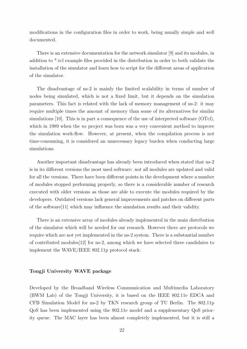
There is an extensive array of modules already implemented in the main distribution
of the simulator which will be needed for our research. However there are protocols we
require which are not yet implemented in the ns-2 system. There is a substantial number
of contributed modules[12] for ns-2, among which we have selected three candidates to
implement the WAVE/IEEE 802.11p protocol stack:
Tongji University WAVE package
Developed by the Broadband Wireless Communication and Multimedia Laboratory
(BWM Lab) of the Tongji University, it is based on the IEEE 802.11e EDCA and
CFB Simulation Model for ns-2 by TKN research group of TU Berlin. The 802.11p
QoS has been implemented using the 802.11e model and a supplementary QoS prior-
ity queue. The MAC layer has been almost completely implemented, but it is still a
22
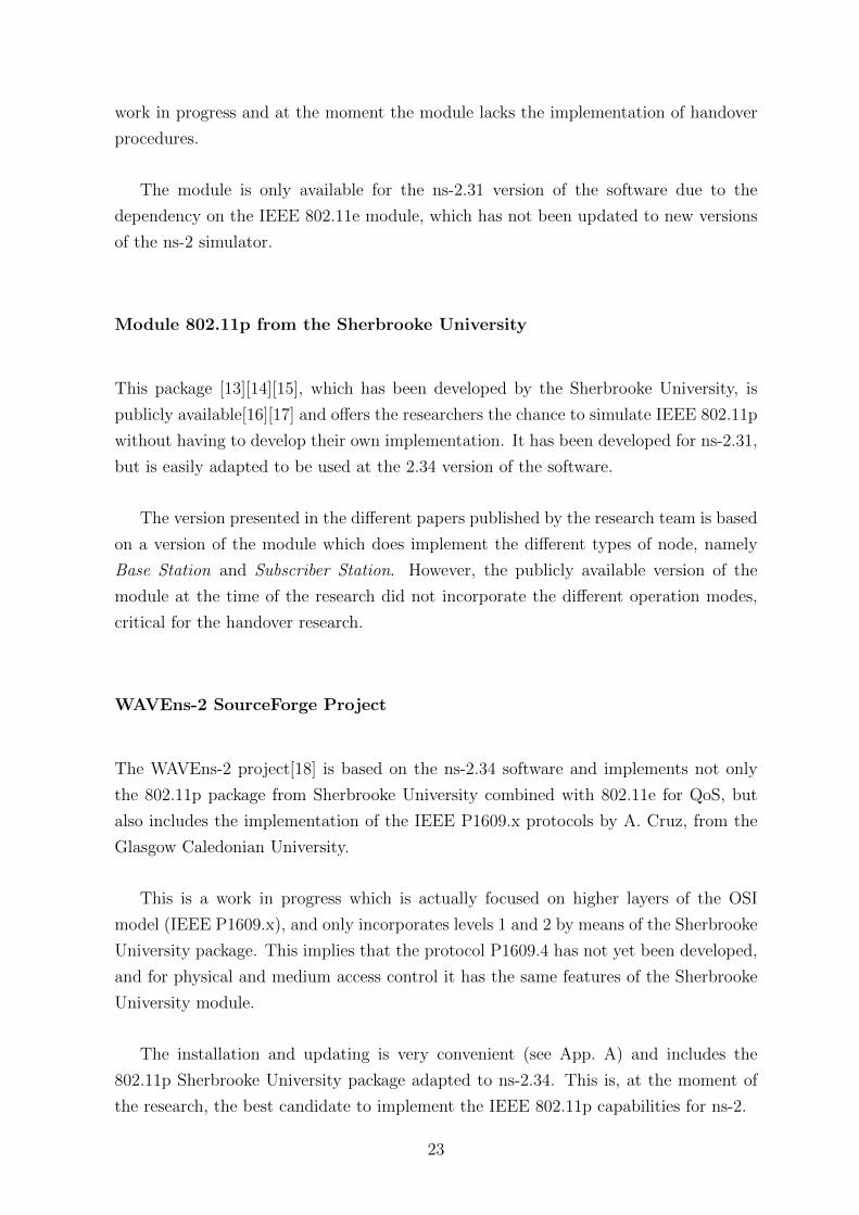
work in progress and at the moment the module lacks the implementation of handover
procedures.
The module is only available for the ns-2.31 version of the software due to the
dependency on the IEEE 802.11e module, which has not been updated to new versions
of the ns-2 simulator.
Module 802.11p from the Sherbrooke University
This package [13][14][15], which has been developed by the Sherbrooke University, is
publicly available[16][17] and offers the researchers the chance to simulate IEEE 802.11p
without having to develop their own implementation. It has been developed for ns-2.31,
but is easily adapted to be used at the 2.34 version of the software.
The version presented in the different papers published by the research team is based
on a version of the module which does implement the different types of node, namely
Base Station and Subscriber Station. However, the publicly available version of the
module at the time of the research did not incorporate the different operation modes,
critical for the handover research.
WAVEns-2 SourceForge Project
The WAVEns-2 project[18] is based on the ns-2.34 software and implements not only
the 802.11p package from Sherbrooke University combined with 802.11e for QoS, but
also includes the implementation of the IEEE P1609.x protocols by A. Cruz, from the
Glasgow Caledonian University.
This is a work in progress which is actually focused on higher layers of the OSI
model (IEEE P1609.x), and only incorporates levels 1 and 2 by means of the Sherbrooke
University package. This implies that the protocol P1609.4 has not yet been developed,
and for physical and medium access control it has the same features of the Sherbrooke
University module.
The installation and updating is very convenient (see App. A) and includes the
802.11p Sherbrooke University package adapted to ns-2.34. This is, at the moment of
the research, the best candidate to implement the IEEE 802.11p capabilities for ns-2.
23

3.2.2 ns-3
Even though ns-3 has been under active development since 2006, ns-2 has not stopped
its development and presence in the research community. ns-3 is actually intended as
an eventual replacement of ns-2. However, it is not an evolution of ns-2: it is a new
simulator. There are a series of problems on ns-2 that ns-3 focused on solving:
• interoperability and coupling between models
• lack of memory management
• debugging of split language objects
As ns-3 had to become such a breakthrough it required different architecture than ns-
2, so it lacks backwards-compatibility with it. There are plenty of community-developed
modules which have not yet been developed for ns-3, and there are high chances that
some will not be ported. This is the reason why ns-2 is still one of the reference simu-
lators, and ns-3 is not yet so popular among researchers.
The main difference for researchers who do not require developing their own modules
is the setup procedure: it was an OTcl script in ns-2 and ns-3 uses C++ with optional
python bindings. The fact that python binding usage is not available for all the possible
ns-3 installations is also to be considered. For the reasons here stated is clear that
switching to ns-3 is a process of re-engineering the simulation scenarios rather than
porting Tcl code to C++.
For developers the difference between using ns-2 or ns-2 is more drastic, not only
because the APIs are not compatible, preventing from a direct implementation, but also
as one of the aims of ns-3 is to improve the interoperability between modules, feature that
ns-2 lacks where the interoperability requires the manual configuration and adoption of
the different files by the user. This is the reason why the development has to follow a
series of conventions and is encouraged to do it as part of the established development
community via an available mercury repository. This ensures the interoperability and
the validation of the different modules by as many developers as possible. Furthermore,
some of this modules will possibly implemented in following All-in-One distributions.
According to the developers it is still a work in progress, but they consider it able
to provide valid simulation results, and its use for research is encouraged. ns-3 has an
extensive array of documentation for both users and developers [19][20][21].
24

3.3 Integrated Mobility and Network Simulators
Integrated simulators have the advantage of being able to modify the traffic parameters
depending on the information traffic among the vehicles and vice versa. This can provide
a higher level of realism for VANET simulations which focus on response to accidents
or collisions and the improvements for those situations.
3.3.1 GloMoSim
GloMoSim (Global Mobile Information Systems Simulation Library) is a scalable sim-
ulation environment for wireless and wired network systems. It employs the parallel
discrete-event simulation capability provided by PARSEC. GloMoSim currently sup-
ports protocols for purely wireless networks.
It had been widely used for network simulation but it now lacks the latest protocols
—including IEEE 802.11p— as the last major version, GloMoSim 2.0, was released in
December 2000. After that PARSEC stopped working on freeware software and the
developers released a commercial version of GloMoSim: QualNet. Even though, it is
still possible to download GloMoSim’s source and binary code for academic research.
3.3.2 NCTUns
The approach to the simulation of the NCTUns (National Chiao Tung University Net-
work Simulator)[22] is its main distinguishing feature: it is embedded on the kernel of
the operating system in order to be able to simulate and emulate networks via the direct
interaction with the system network protocol stack or use any application available to
generate traffic. For that reason the only operating system supported by the developers
for the latest NCTUns 6.0 is Red Hat’s Fedora 12.
The installation in the supported system is well documented and straightforward
even when performed over a virtual machine, method used to test this system for this
research. Other Linux distributions such as Ubuntu may work with NCTUns as they
use the same Linux kernel as Fedora. However, this other systems are not supported
and the proper configuration must be checked using the validation tests provided.
The main drawback of this solution is the lack of flexibility in terms of module con-
figuration and its very slow workflow: It is completely based on a graphical interface,
25

preventing the fast and convenient modification of parameters to run statistically inde-
pendent simulations or changing configurations from one iteration to the next in order
to sweep the different simulation variables.
On the other hand, the graphical user interface [23] together with the demo videos
[24] prove to be a very convenient way to allow the configuration of simulations with an
almost inexistent learning curve.
3.3.3 OMNeT++
OMNeT++ is an object-oriented discrete event network simulator. It can be further
extended by means of modules, which may be nested unlimited times. Its framework
offers the possibility to have its features and simulation capabilities expanded as long
as its possible to create the C++ code that implements the modules. This flexibility
implies that OMNeT++ is not limited to network simulators, but any other kind of
modeling that can be implemented using C++.
OMNeT++ is based on C++ modules, which are distributed and connected using
NED topology description language. It can be executed via an IDE based on Eclipse
platform, which is convenient for set-up and for running small simulations and also
can be used via command-line, providing a fast and convenient simulation method for
complex or batched simulations.
Some of the features of OMNeT++ are:
• hierarchically nested modules
• topology description language
• modules communicate with messages through channels
• flexible module parameters
The installation is available for the main operating systems and it proves to be
straightforward and hassle-free.
A critical disadvantage is the lack of mobility management as an integrated part of
the simulator, requiring the installation of frameworks in order to provide that key func-
tionality in VANET simulations. There is mainly one contributed framework available
for OMNeT++ which focuses in VANET networks:
26

MiXiM module
MiXiM (mixed simulator)[25] is a modeling framework for mobile and fixed wirelessnet-
works. It offers detailed physical and MAC layer models, such as radio wave propaga-
tion, interference estimation, radio transceiver power consumption and wireless MAC
protocols, with IEEE 802.11p among others.
However, it mainly focuses on the implementation of existing wireless network inter-
face cards (NICs), fact which constrains the researcher’s configuration options in order
to optimize the protocol using any available strategy.
INET Framework
The INET Framework[26] is an open-source communication networks simulation package
for OMNeT++. The INET Framework contains models for several wired and wireless
networking protocols, including IEEE 802.11p. However, it focuses on the modeling of
higher levels of the protocol architecture.
Mixnet: MiXiM + INET
MiXiM provides very detailed models of wireless NICs, but on the other hand it does
not implement very sophisticated upper layers. As these are the layers for which the
INET framework provides a lot of very detailed modules, Mixnet[27] combines these
modules complementing their strengths.
3.3.4 Commercial Solutions
Most of the commercial software available for network simulation consider the simulators
from an industrial research point of view, hence focused on issues such as support for
certain devices, quality of human support, etc., which are less relevant for academic
researchers. At the same time, this solutions usually lack the configuration possibilities
in terms of protocol features, key aspect for research.
However, commercial solutions deserve to be mentioned, but will not be tested and
therefore not evaluated as candidates for this research. Some of the most well-known
network simulation frameworks are: MapleSim, simulator from the developers of the
well-known Maple Mathematics software; NetSim; OMNEST, the commercially sup-
ported version of OMNeT++, required for commercial purposes; OPNET and QualNet,
the commercial version of the previously mentioned GloMoSim.
27

3.4 Federated solutions
This solutions use a software integrating one of each kind of the aforementioned spe-
cialized simulators. This solutions implement the required features by means of at least
two simulators which have compatible or translatable output/input files. In the VANET
world any simulation would require the use of two specialized simulators: one for mo-
bility and another for networking. Additionally this software may require the use of
translation scripts for the mobility traces to be used as input for the network simulator.
3.4.1 SUMO/ns-2
This combination provides a common framework for research. As part of the SUMO
project there is a trace translator tool called TraceExporter which provides researchers
with the interface to combine the two systems. TraceExporter is easy to use but while
testing a coding mistake was found which produced negative coordinates, probably
produced because road width was not properly taken into account. This prevented ns-2
to use the translated traces. It was easily solved by means of adding an offset for all the
coordinates into the translation code.
Rapid Generation of Realistic Simulation for VANET
This software [8] offers the users of SUMO and ns-2 or QualNet a very easy to use
java graphic interface. It is an evolution of the MOVE project which now includes the
interoperability with the network simulator. The mobility generation in this software is
still referred to as MOVE.
This software is still limited by the previously mentioned features of the simulation
software it relies on and even more, as it does not allow to reach all the potential of
either of the software involved through its configuration wizards, specially in the network
simulation aspect. It lacks the flexibility required to make complex simulations, but it
may be convenient for scenario generation when the user is not yet confident with
command-line configuration.
TraNS
TraNS (Traffic and Network Simulation Environment) is also a java GUI for SUMO and
ns-2 interaction using the TraCI output interface provided by the developers of SUMO.
28
It requires specific versions of both SUMO and ns-2, and it has not been updated for
the last versions of the different components.
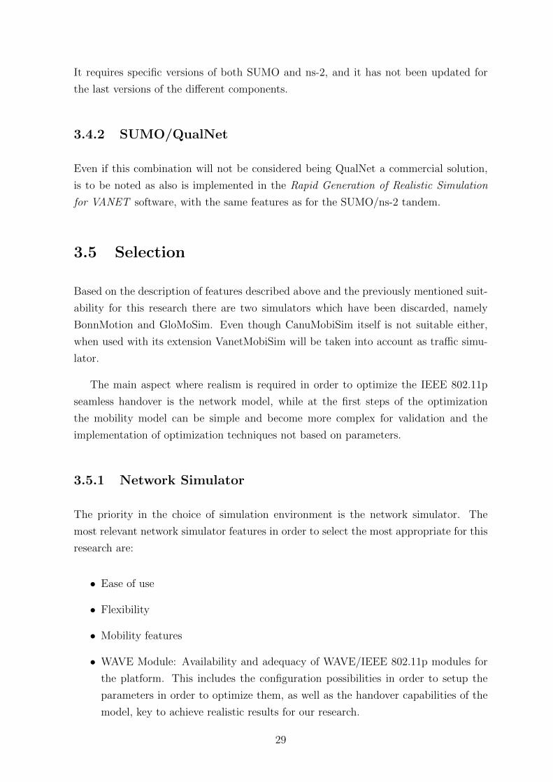
3.4.2 SUMO/QualNet
Even if this combination will not be considered being QualNet a commercial solution,
is to be noted as also is implemented in the Rapid Generation of Realistic Simulation
for VANET software, with the same features as for the SUMO/ns-2 tandem.
3.5 Selection
Based on the description of features described above and the previously mentioned suit-
ability for this research there are two simulators which have been discarded, namely
BonnMotion and GloMoSim. Even though CanuMobiSim itself is not suitable either,
when used with its extension VanetMobiSim will be taken into account as traffic simu-
lator.
The main aspect where realism is required in order to optimize the IEEE 802.11p
seamless handover is the network model, while at the first steps of the optimization
the mobility model can be simple and become more complex for validation and the
implementation of optimization techniques not based on parameters.
3.5.1 Network Simulator
The priority in the choice of simulation environment is the network simulator. The
most relevant network simulator features in order to select the most appropriate for this
research are:
• Ease of use
• Flexibility
• Mobility features
• WAVE Module: Availability and adequacy of WAVE/IEEE 802.11p modules for
the platform. This includes the configuration possibilities in order to setup the
parameters in order to optimize them, as well as the handover capabilities of the
model, key to achieve realistic results for our research.
29
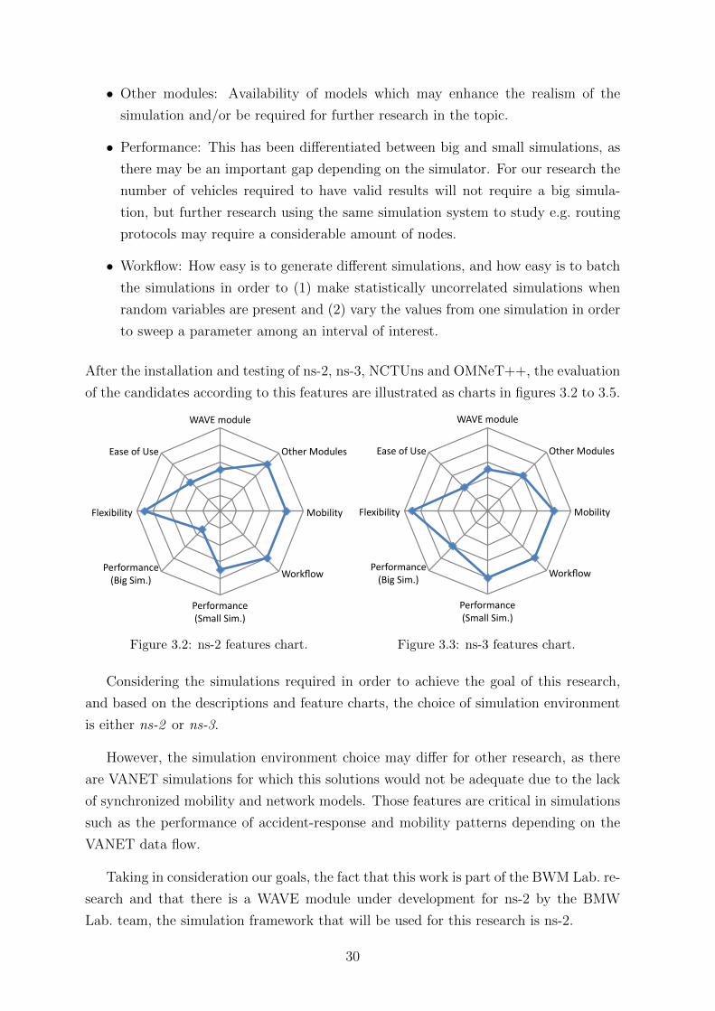
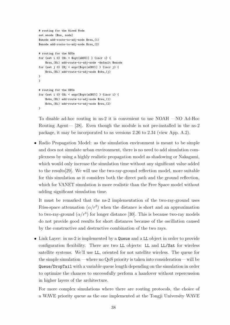
• Other modules: Availability of models which may enhance the realism of the
simulation and/or be required for further research in the topic.
• Performance: This has been differentiated between big and small simulations, as
there may be an important gap depending on the simulator. For our research the
number of vehicles required to have valid results will not require a big simula-
tion, but further research using the same simulation system to study e.g. routing
protocols may require a considerable amount of nodes.
• Workflow: How easy is to generate different simulations, and how easy is to batch
the simulations in order to (1) make statistically uncorrelated simulations when
random variables are present and (2) vary the values from one simulation in order
to sweep a parameter among an interval of interest.
After the installation and testing of ns-2, ns-3, NCTUns and OMNeT++, the evaluation
of the candidates according to this features are illustrated as charts in figures 3.2 to 3.5.
!"#$%&'()*+%
,-.+/%0'()*+1%
0'23*3-4%
!'/56'7%
8+/9'/&:;<+%=>&:**%>3&?@%
8+/9'/&:;<+%=A3B%>3&?@%
C*+D323*3-4%
$:1+%'9%E1+%
Figure 3.2: ns-2 features chart.
!"#$%&'()*+%
,-.+/%0'()*+1%
0'23*3-4%
!'/56'7%
8+/9'/&:;<+%=>&:**%>3&?@%
8+/9'/&:;<+%=A3B%>3&?@%
C*+D323*3-4%
$:1+%'9%E1+%
Figure 3.3: ns-3 features chart.
Considering the simulations required in order to achieve the goal of this research,
and based on the descriptions and feature charts, the choice of simulation environment
is either ns-2 or ns-3.
However, the simulation environment choice may differ for other research, as there
are VANET simulations for which this solutions would not be adequate due to the lack
of synchronized mobility and network models. Those features are critical in simulations
such as the performance of accident-response and mobility patterns depending on the
VANET data flow.
Taking in consideration our goals, the fact that this work is part of the BWM Lab. re-
search and that there is a WAVE module under development for ns-2 by the BMW
Lab. team, the simulation framework that will be used for this research is ns-2.
30

!"#$%&'()*+%
,-.+/%0'()*+1%
0'23*3-4%
!'/56'7%
8+/9'/&:;<+%=>&:**%>3&?@%
8+/9'/&:;<+%=A3B%>3&?@%
C*+D323*3-4%
$:1+%'9%E1+%
Figure 3.4: NCTUns features chart.
!"#$%&'()*+%
,-.+/%0'()*+1%
0'23*3-4%
!'/56'7%
8+/9'/&:;<+%=>&:**%>3&?@%
8+/9'/&:;<+%=A3B%>3&?@%
C*+D323*3-4%
$:1+%'9%E1+%
Figure 3.5: OMNeT++ features chart.
3.5.2 Mobility Simulator
The choice of traffic simulator for our research has been reduced to two candidates:
SUMO and VanetMobiSim. For the simulations required for this research it is not
needed to perform complex mobility simulations, and both systems have a set of features
which exceed our requirements. Both frameworks provide a wide array of configurations,
including both real and artificial layouts, multi-lane roads, influence of traffic signs,
etc. and can export their mobility traces as ns-2 format.
Hence, the choice of traffic simulator is not critical between our two candidates and
it will become a choice of the researcher who may even choose one simulator or the other
according to each particular simulation requirements.
31


Chapter 4
Handover Optimization
In this chapter the network parameters involved in the optimization of the handover
process will be presented. The focus will be the explanation of each parameter involved
in the handover performance, the selection criteria of the ones we will use to optimize
the performance, the simulation values that will be evaluated as well as the procedure
to configuring the simulation in the selected simulation environments.
Strategies for further optimization will also be presented as leads for further research
on the VANET seamless handover improvement in terms of latency and performance.
4.1 Parameter Optimization
4.1.1 Procedure
In order to optimize the handover process by means of the parameter value selection
the procedure has been the following:
1. identification of the network parameters that will allow a faster and more reliable
handover when optimized.
2. design and generation of simple models to test the parameters values, as first
approach to optimizing the system.
The simulation scenarios are:
• wired-cum-wireless 802.11p scenario: hierarchical addressing including differ-
ent infrastructure levels. This simulates the access to a remote server from
the mobile nodes and allows the study of the handover performance.
33

• Mobile IP wired-cum-wireless 802.11p scenario: hierarchical addressing with
one of the IEEE 802.11p infrastructure nodes acting as Home Agent and the
rest as Foreign Agents.
3. generation of complex models. Validate and rectify the results of step number 2.
4.1.2 Simulation Scenario
There are some general parameters in any given simulation which will determine the
environment characteristics and will influence in the results of the simulations. For
the optimization of the handover to be valid is required that this parameters have a
minimum impact in the results.
The design of the simulation may eventually reduce the level of realism of the results
of the simulation, but will allow fast batched simulations to define the values, which
afterwards will be applied in more complex scenarios where the optimized values will
be validated. The selection of the non-strictly IEEE 802.11p parameters defining the
environment for the simulation and their descriptions are:
• Node layout and movement pattern: The layout is as seen in fig. 4.1. There are
nOBU vehicles at distance obuD proceeding along the straight way at average speed
obuS. The real speed will be a normal random number centered in obuS and a
standard deviation of a 5% of this value. The road has two infrastructure nodes
at a distance rsuD. The latter are connected to a server.
This layout has been chosen to make the simulations with multiple vehicles in
order to make a more realistic physical layer response for different vehicle load.
The implementation is not complex, thus the choice is to implement it directly
on the ns-2 configuration script file with no need to use any third party mobility
simulation software.
The solution presented has the advantage of being easily modified to create batched
simulations via scripting and using command-line arguments:
# Layout configuration
# set layout and mobility patterns
set opt(rsuD) rsuD ;# distance between RSUs (m)
set opt(obuS) obuS ;# average vehicle speed (m/s)
set opt(obuD) obuD ;# starting distance between vehicles (m)
;# recommended value ~obuS/4 (safety braking distance)
# set floor size
set opt(x) expr[$opt(rsuD)+2*1200] \
34

rsuD
obuD
obuD
obuD
obuD
obuD
obuD
obuD
obuD
obuD
obuD obuS
obuD
Figure 4.1: Simple simulation layout.
;#distance required to prevent having signal at the OBUs starting point
set opt(y) 500
# define topology
set topo [new Topography]
$topo load_flatgrid $opt(x) $opt(y)
# number of nodes
set opt(nRSU) 2
set opt(nOBU) expr[$opt(x)/$opt(rsuD)]
# set start/stop time
set opt(start) 0.0
set opt(stop) expr[$opt(x)/$opt(obuS)+$opt(nOBU)*$opt(obuD)/$opt(obuS)]
# set RNG for speed
set obuSRNG [new RNG]
for {set j 1} {$j < $run} {incr j} {
$obuSRNG next-substream
}
# obuS_ is a exponential random variable describing the time
# between consecutive packet arrivals
set obuS_ [new RandomVariable/Normal]
$obuS_ set avg_ $obuS
$obuS_ set std_ expr[$obuS*0.05]
$obuS_ use-rng $obuSRNG
# ======================================================================
# Main Program
# ======================================================================
#
35

# Initialize Global Variables
#
# create simulator instance
set ns_ [new Simulator]
#
# Create God
#
set god_ [create-god expr[$opt(nRSU)+$opt(nOBU)]]
#
# Create the specified number of nodes
#
# create Wired Node
set wnode [$ns_ node]
$wnode random-motion 0
# create RSUs
for {set i 0} {$i < $opt(nRSU)] } {incr i} {
set rsu_($i) [$ns_ node]
$rsu_($i) random-motion 0
}
# create OBUs
for {set i 0} {$i < expr[$opt(nOBU)] } {incr i} {
set obu_($i) [$ns_ node]
$obu_($i) random-motion 0
}
#
# mobility
#
$wnode set X_ expr[$opt(x)/2]
$wnode set Y_ 350.0
$wnode set Z_ 0.00
$rsu_(0) set X_ expr[($opt(x)-$opt(rsuD))/2]
$rsu_(0) set Y_ 250.0
$rsu_(0) set Z_ 0.00
$rsu_(1) set X_ expr[($opt(x)+$opt(rsuD))/2]
$rsu_(1) set Y_ 250.0
$rsu_(1) set Z_ 0.00
for {set i 0} {$i < $opt(nRSU) } {incr i} {
$obu_($i) set X_ 0.00
$obu_($i) set Y_ 250.0
$obu_($i) set Z_ 0.00
}
# OBUs movement
for {set i 0} {$i < expr[$opt(nOBU)] } {incr i} {
36

$ns_ at expr[$i*$opt(obuD)/$opt(obuS)] \
"$obu_($i) setdest $opt(x) 250.00 expr[$obuS_ value]"
}
$ns_ initial_node_pos $wnode 150
for {set i 0} {$i < $opt(nRSU) } {incr i} {
$ns_ initial_node_pos $rsu_($i) 100
}
for {set i 0} {$i < $opt(nOBU) } {incr i} {
$ns_ initial_node_pos $obu_($i) 20
}
#
# Tell nodes when the simulation ends
#
$ns_ at $opt(stop).1 "$wnode reset";
for {set i 0} {$i < $opt(nRSU) } {incr i} {
$ns_ at $opt(stop).1 "$rsu_($i) reset";
}
for {set i 0} {$i < $opt(nOBU) } {incr i} {
$ns_ at $opt(stop).1 "$obu_($i) reset";
}
$ns_ at $opt(stop).001 "finish"
#Define ’finish’ procedure
proc finish {} {
$ns_ flush-trace
close $tracefd
puts "NS EXITING..."
$ns_ halt
}
puts "Starting Simulation..."
$ns_ run
• Routing Protocol: there are a variety of available ad-hoc routing protocols in ns-
2, namely DIFFUSION/RATE, DIFFUSION/PROB, DSDV, DSR, FLOODING,
OMNIMCAST, AODV, TORA and PUMA. However, in our simulation, as we
configured the topology with multiple mobile nodes, for the analysis of handover
it is more convenient not to use any ad-hoc routing protocol and create the routing
tables manually for all the mobile nodes in order to restrict the connection from
the mobile node to the wired node exclusively via either of the infrastructure nodes
directly, with no multi-hopping between OBUs.
The manual routing configuration would require the following code:
# Manual routing with expanded addresses (21 bits nodes).
$ns_ rtproto Manual
$ns_ set-address-format expanded
37
# routing for the Wired Node
set wnode [$ns_ node]
$wnode add-route-to-adj-node $rsu_(1)
$wnode add-route-to-adj-node $rsu_(2)
# routing for the RSUs
for {set i 0} {$i < $opt(nRSU)] } {incr i} {
$rsu_($i) add-route-to-adj-node -default $wnode
for {set j 0} {$j < expr[$opt(nOBU)] } {incr j} {
$rsu_($i) add-route-to-adj-node $obu_(j)
}
}
# routing for the OBUs
for {set i 0} {$i < expr[$opt(nOBU)] } {incr i} {
$obu_($i) add-route-to-adj-node $rsu_(1)
$obu_($i) add-route-to-adj-node $rsu_(2)
}
To disable ad-hoc routing in ns-2 it is convenient to use NOAH —NO Ad-Hoc
Routing Agent— [28]. Even though the module is not pre-installed in the ns-2
package, it may be incorporated to ns versions 2.26 to 2.34 (view App. A.2).
• Radio Propagation Model: as the simulation environment is meant to be simple
and does not simulate urban environment, there is no need to add simulation com-
plexness by using a highly realistic propagation model as shadowing or Nakagami,
which would only increase the simulation time without any significant value added
to the results[29]. We will use the two-ray-ground reflection model, more suitable
for this simulation as it considers both the direct path and the ground reflection,
which for VANET simulation is more realistic than the Free Space model without
adding significant simulation time.
It must be remarked that the ns-2 implementation of the two-ray-ground uses
Friss-space attenuation (α/r2) when the distance is short and an approximation
to two-ray-ground (α/r4) for longer distance [30]. This is because two-ray models
do not provide good results for short distances because of the oscillation caused
by the constructive and destructive combination of the two rays.
• Link Layer: in ns-2 is implemented by a Queue and a LL object in order to provide
configuration flexibility. There are two LL objects: LL and LL/Sat for wireless
satellite systems. We’ll use LL, oriented for not satellite wireless. The queue for
the simple simulation —where no QoS priority is taken into consideration— will be
Queue/DropTail with a variable queue length depending on the simulation in order
to optimize the chances to successfully perform a handover without repercussion
in higher layers of the architecture.
For more complex simulations where there are routing protocols, the choice of
a WAVE priority queue as the one implemented at the Tongji University WAVE
38
package or Queue/DropTail/PriQueue should be considered, as it has a flag imple-
mented (Prefer Routing Protocols) to give priority to routing packages —which
are inexistent in previous simulations— and could be expected to have an overall
improvement, and specifically in the handover performance.
• Antennas: Omni-directional antennas with unity gain (for both transmission and
reception) which are centered in the node and 1.5 meters above it.
• Traffic: The simulated data traffic will be in both upstream and downstream.
From the RSUs side there will be broadcasting of periodic packages simulating
the security information spread, and allowing us to calculate the real downstream
handover latency. From the mobile nodes, and to be able to calculate the real up-
stream and bidirectional handover latency, there will be a constant bit-rate agent
trying to transmit unicast packages to the server connected to both infrastructure
nodes. As there is no ad-hoc routing configured the only chance that this packages
will arrive to their destination is that the nodes are attached to the corresponding
infrastructure-enabled node.
4.1.3 Simulation Parameters
The WAVE standard fixes a series of parameters for both IEEE 802.11p physical layer
(PHY) and medium access control layer (MAC) in order to ensure interoperability, as
introduced in chapter 2. In table 4.1 the PHY parameters are described, while the
standardized MAC IEEE 802.11p parameters involved in the simulation are the ones in
the table 4.3.
On the other hand, and as also stated at chapter 2, WAVE aims at enabling com-
munication between nodes by defining the minimum set of parameters. For this reason
there are a series of parameters described at table 4.4 which are available for the devel-
oper to implement proper values as considered for the design requirements.
Among the table 4.4 parameters there are some which are not intrinsically involved
in the handover process optimization and not to be considered to be optimized, namely
CP ratio, preamble length, and PLCP Header length and data rate.
39

Parameter Description Value
Transmission RangeMaximum communication range
1000 mbetween OBU and RSU
CSThresh Wireless interface sensitivity -85 dBm
Pt Transmission Power 20 dBm
Data Rates in Mbps 3 to 27
Frequency 5.9 × 10⁹
Noise floor for 10MHz bandwidth -99 dBm
L radio circuit gain/loss ratio 1.0
PowerMonitorThresh Power monitor sensitivity -102 dBm
HeaderDuration 40 µs
ModulationSchemeThe modulation is set according to
Table 4.2the different data rates.
SINR PreambleCaptSignal to Interference and Noise Ratio
4 dBfor preamble capture.
SINR DataCaptSignal to Interference and Noise Ratio
10 dBfor data capture.
Channel Physical medium Wireless
BW Bandwidth 10 MHz
FFT
Fast Fourier Transform size 64Fast Fourier Transform period 6.4 µsGuard Interval Duration 1.6 µs (6.4/4)Symbol interval 8 µs (6.4+1.6)
Sub-carriers
Number of data subcarriers 48Number of pilot sub-carriers 4Total number of sub-carriers 52Sub-carrier frequency spacing 0.15625 Mhz
Signal BW Signal Bandwidth 8.28 MHz
Table 4.1: PHY layer parameters and standardized values.
Data Rate Modulation Encoding ratebits per bits per symbol
sub-carrier Coded Data
3 BPSK 1/2 1 48 24
4.5 BPSK 3/4 1 48 36
6 QPSK 1/2 2 96 48
9 QPSK 3/4 2 96 72
12 QAM-16 1/2 4 192 96
18 QAM-16 3/4 4 192 144
24 QAM-64 2/3 6 288 192
27 QAM-64 3/4 6 288 216
Table 4.2: Signal structure for OFDM depending on the data rate.
40

Parameter Description Value
CWmin Minimum Contention Window for congestion control. Table 2.1
CWmax Maximum Contention Window for congestion control Table 2.1
AIFSN Arbitrary Inter-Frame Space Number Table 2.1
AIFS Arbitrary Inter-Frame Space (AIFSN × Slot T ime+ SIFS ) Table 2.1
Slot Time 13µs
SIFS Short Inter-Frame Space 32µs
Short Retry Limit Retry limit for short MAC Layer frames 7
Long Retry Limit Retry limit for long MAC Layer frames 4
RTS Theshold Limit between Short and Long frames 2346b
Header Duration 40µs
Symbol Duration 8µs
Table 4.3: MAC layer parameters and standard values required to ensure interoperability.
Parameter Description
QoS Class QoS Class for the handover related communications.
Beacon Interval time interval between beacon transmissions.
Preamble Length
PLCP Header Length Physical-Layer Convergence Procedure Header Length
PLCP Data Rate Physical-Layer Convergence Procedure Data Rate
Scanning Mode Active or passive mode, as explained in section 2.4.2.
Probe Delay
As explained in section 2.4.2Max Channel TimeMin Channel TimeChannel Time
CP Ratio OFDM: Ratio of the Cyclic Prefix time over useful time.
Table 4.4: Parameters available for design.
41

Handover Parameters
Of those parameters that have been introduced in the previous section, those directly
involved in the handover optimization process are listed in table 4.5, together with the
values used as starting point for the optimization.
Parameter Starting value
Scanning Mode PASSIVE
Beacon Interval 300ms
Probe Delay 10ms
Min Channel Time 20ms
Max Channel Time 50ms
Channel Time 300ms
Table 4.5: Default simulation values for IEEE 802.11p handover optimization.
Even though this values will be modified in order to optimize the handover process,
there are some restrictions that should be taken into account, such as the ChannelTime
relation to BeaconInterval, as explained in section 2.4.2. Another critical consideration
is the choice of MinChannelTime, which should fulfill:
MinChannelT ime ≥ SIFS + (2 + CWmin) × SlotT ime
42

4.2 System Configuration
4.2.1 ns-2 Simulation Scripts
All the presented scripts are meant to be batch-executed, as there are a number of pa-
rameters we want to improve and we need to make simulations with different parameter
interval and granularity. To be able to acquire results as soon as the system is properly
configured a bash script has been developed to allow the batched simulation and analysis
of the results of the provided ns-2 tcl scripts, which can be found in App. B.
Scripting considerations
Module: As shown in chapter 3, at the time this research took place there was no
available 802.11p module which included all the required features. As the Sherbrooke
University is the most documented for those features [13] we will use the described
syntax to develop our simulation scripts.
However, the 802.11p module from Sherbrooke University is developed and tested
for ns-2.31. As it has been adapted to implement the lower layers in WAVEns-2 project,
which is based on ns-2.34, we will use the latter, which provides ns-2.34 compatibility
for the Sherbrooke University package1 and higher layer implementation of the WAVE
architecture.
Random Variables: In [31] is proved how the set up of random number generation
and the selection of seeds for the different simulation runs will be critical to achieve
uncorrelated results among their outputs. It is estimated that due to the re-utilization of
scripts based on the old random number generator (RNG) syntax, which was deprecated
in version 2.1b9, up to 80% of the published results achieved using ns-2 as network
simulator might be affected by relatively-high correlated results from different runs.
For the ns-2 RNG the incorrect and proper [9] syntaxes to be used are the following:
• ns-2 incorrect RNG use.
# Usage: ns bad-rng-test.tcl [seed1 value] [seed2 value]
if {$argc > 2} {
puts "Usage: ns bad-rng-test.tcl \[seed1 value\] \[seed2 value\]"
puts "For random seed use 0"
exit
}
1Future versions of the Sherbrooke University package will be included in the WAVEns-2 project.
43

set seed1 0
set seed2 0
if {$argc == 2} {
set seed1 [lindex $argv 0]
set seed2 [lindex $argv 1]
}
if {$argc < 2} {
puts "No seeds introduced, using 0 as seed1 and seed2"
set seed1 0
set seed2 0
}
# create the RNGs and set the seed
set firstRNG [new RNG]
$firstRNG seed $seed1
set secondRNG [new RNG]
$secondRNG seed $seed2
• ns-2 proper RNG use.
# Usage: ns rng-test.tcl [replication number]
if {$argc > 1} {
puts "Usage: ns rng-test.tcl \[replication number\]"
exit
}
set run 1
if {$argc == 1} {
set run [lindex $argv 0]
}
if {$run < 1} {
set run 1
puts "No replication number introduced, assuming 1st run"
}
# create the RNGs and set them to the correct substream
# appropriate RNG seeds are assigned automatically
set firstRNG [new RNG]
set secondRNG [new RNG]
for {set j 1} {$j < $run} {incr j} {
$firstRNG next-substream
$secondRNG next-substream
}
4.2.2 Batched simulation
A script has been prepared to configure and run the ns .tcl files available in App. B
as batched simulations. Furthermore, the user may chose whether to automatically
calculate the statistics as described in section 4.2.3.
44
The parameters available for configuration using this script are:
Network parameters:
• ScanType either ACTIVE, PASSIVE or BOTH
• BeaconInterval fixed value or interval with configurable steps (in ms)
• ProbeDelay fixed value or interval with configurable steps (in ms)
• MinChannelTime fixed value or interval with configurable steps (in ms)
• MaxChannelTime fixed value or interval with configurable steps (in ms)
• ChannelTime fixed value or interval with configurable steps (in ms)
Mobility parameters (According to the description in section 4.1.2)
• rsuD fixed value or interval with configurable steps (in m)
• obuS fixed value or interval with configurable steps (in m/s)
• obuD fixed value or interval with configurable steps (in m)
Other parameters
• Iterations number of runs per simulation (integer > 0)
• route trace file route for the current run (string)
The actual script, its interface together with the design and expansion considerations
can be found in App. C.
45
4.2.3 Performance evaluation
The main aspects that will allow us to detect an improvement in terms of handover
performance are the throughput (average), transmission delay (minimum, maximum
and average), overall handover latency and ratio for received/sent and dropped/sent
packets.
The analysis of the traces will be automatically performed upon request during the
execution of the batch script generator, and uses the scripts described and available in
App. C.2.
The output of the performance evaluation is stored in a series of files as follows:
• one file for each step of the simulation, including the values of each individual run
for the mentioned parameters.
• one file per batched execution which includes the statistic study for each step of
the batched simulation.
• one file per batched execution which indicates for each of the performance indica-
tors which is the best parameter choice among the simulations executed.
46

4.3 Strategies for further optimization
In this section different strategies that may be used to further improve the handover
performance will be introduced. This strategies do not rely on the accurate parameter
adjustment in order to improve the results, instead they rely on the use of context
information, protocol features, etc. in order to maximize the chances of successfully
handover within the minimum period of time since the de-association from the previous
infrastructure node.
Most of this strategies require some conditions to be valid, as usually they will focus
in optimizing one aspect of the process in expense of performance with techniques that
for example assume the risk of not receiving some potentially relevant data or that
reduce the number of RSUs considered handover candidates.
4.3.1 Trigger optimization
As already introduced in section 2.4.1, the choice of the proper triggers —considering
both network and mobility parameters— leads to an optimization of the overall handover
performance. Another issue, very relevant in VANETs is when to decide not to trigger
the handover, even if some parameters would indicate to do so.
In an environment where the vehicles —mainly public transport vehicles— can act
as access points in a pseudo-RSU manner (mobile RSUs), the chances that the network
parameters would indicate to handover may not be the optimum, as mobility factors
such as the relative speed between the OBU and the RSU which manages the WBSS
may indicate that the same WBSS you belong is the most convenient.
Considering a situation where there are overlapping networks and the vehicle is in an
intermediate point between the RSUs: there may be moments when constant handover
between two RSUs would be indicated by the network parameters. In those situations
is important that the RSU decides not to handover, as it would increase considerably
the latency and packet loss chances. This approach requires the implementation of a
hysteresis, that prevents the constant handover when the choice between RSUs may
fluctuate constantly.
4.3.2 Choice of RSU for the handover
The choice of RSU is clearly a topic that will have an impact on the long-term network
performance, as a good choice will provide service during a longer period of time, re-
47

ducing the signaling overhead and probability of data loss and link breaks introduced
when performing a handover.
The aspects to consider in order to choose the most convenient RSU include the
services provided by the RSU —security messages, internet connectivity, etc.—, network
parameters —SNR, QoS, medium access availability, etc.— and mobility parameters —
distance, relative speed, acceleration, path, etc.—.
4.3.3 Implementation of MIH
and Cross-Layer Communication
Cross-layer communications and Media Independent Handover are, as explained in sec-
tions 2.7 and 2.8 respectively, technologies which may introduce improvements to the
handover performance and new capabilities [32][33][34][35][36][37].
4.3.4 Reducing the Discovery Latency
Discovery latency is the factor with more contribution to the handover latency which
may be responsible for up to the 90% of the process latency [32][38]. For this reason
the impact of reducing it will imply a considerable reduction of the handover process.
Considering a contribution of 90%, if a method was able to reduce the discovery time
in a 20% it would reduce the whole handover latency in a 18%.
Therefore the minimization of the discovery latency is considered a priority when
optimizing the handover process, as it practically implies the minimization of the whole
handover latency. To achieve this we present the following approaches:
Suppressing the scan phase
In most of the IEEE 802.11 protocols it is required to scan all the channels trying to
find an access point, as they can be configured to give service at any channel. When
using WAVE mode on IEEE 802.11p, the RSUs are always advertising at the channel
178, as explained at section 2.5.
In [39] this approach is considered, based on the assumption that the WAVE mode
is active, the RSUs transmission ranges do not overlap as the choice is the first detected
network.
48

This approach does not allow the implementation of seamless handover, as WAVE
mode is required and the transmission ranges are to be considered separated arbitrarily.
Interleaving data and scan packets
For those situations where WAVE mode is not used, and in order to reduce the discovery
latency when there are networks overlapping, part of the scan phase can be performed
while associated to an AP, potentially reducing the impact of the scan phase to zero[38].
4.3.5 Using mobility/environment parameters
There are a series of assumptions that can be made when considering handover between
RSUs in a VANET which are not related to network aspects but mobility. This will
allow tailored solutions depending on the applicable conditions to any given situation.
In VANETs there are high chances that the involved vehicles have access to their
speed and their geographical position through a GPS receiver. At the same time,
VANET nodes are bound to a predefined road network. This is to be assumed for
all the mobility-based enhancement strategies.
Using the information available from the GPS and the fact that VANET nodes are
bound to a already known road network their freedom of movement is drastically reduced
allowing the path calculation of the different nodes with a relatively high accuracy. As
RSUs are usually static and placed strategically along a road, the number of RSUs that
are appropriate for a handover is limited and easily predictable.
This could be even extended when considering mobile RSUs. This vehicles have a
very predictable route, and even though the exact location at a given time may not be
known beforehand there are techniques which may be used in order to broadcast the
location of the closest mobile RSUs, such as neighbor discovery.
Neighbor Discovery
As presented in [34][37][40], oncoming vehicles may broadcast the location of the last
RSU they were attached to. This approach optimizes the handover performance based
on the data exchange of the connectivity parameters and the distance to potential RSUs
to handover to, allowing the OBU to prepare to handover with a prediction of the gap
between RSUs, the channel to scan in order to find the next RSU and further information
which may increase the handover performance.
49

Chapter 5
Conclusions
The research provides the knowledge and the selection, setup and preparation of the
required simulation environment for the study of VANETs, providing a inestimable
starting point for any research focusing on providing seamless handover to IEEE 802.11p-
based VANETs. The delay in research due to the learning curve and preparation of the
simulation environment prior to the achievement of valid results can be overcome by
using this research.
Software tools have been developed in order to provide researchers the capacity to
perform simulations in a batched manner starting at the moment the described simu-
lation framework has been installed and configured, regardless of the familiarity of the
researcher with the aforementioned simulation environment.
The batched approach allows the researcher to generate and execute simulations
leaving the system unattended. During the timespan required to execute all the con-
figured simulations the researcher may focus on other topics while the time-consuming
simulations take place in the background or in a different machine.
Being a system which allows the achievement of valid simulation results as provided,
pre-configured simulations have been implemented in the main program developed for
the simulation setup, and further research simulation scripts can be easily incorporated.
This creates a flexible system that allows the researcher the implementation of their
own environments and introducing them on the developed system, further expanding
its possibilities.
Furthermore, the system developed is able to analyze the results in an automated
manner, providing the statistics and summary of the results once the simulations are
finished, considerably enhancing the research workflow.
51

Introducing further research, different optimization strategies have been proposed,
providing concepts and techniques for further improvements in terms of handover op-
timization. These different approaches may be implemented and subsequently tested
taking advantage of the software presented in this report, taking advantage of its ex-
pansion capabilities.
52

Appendix A
Installation
A.1 ns-2
The easiest installation method for ns-2.34 is by means of the all-in-one package available
in [41], as it includes not only the ns-2.34 package but also some software that will allow
the visualization of traces, creation of graphics, etc.
After this installation and for the purpose of this research it should be considered
to substitute the original ns-2.34 directory with the one of the WAVEns project[18],
available from the svn repository using the following command:
svn co https://wavens-2.svn.sourceforge.net/svnroot/wavens-2 wavens-2
A.2 NOAH - No Ad-Hoc Routing
To install NOAH routing [28] in ns-2 there are some new files and modifications to
existing ones required in order to provide a valid implementation. This tutorial is based
on a ns-2.34 version installed as presented in App. A.1. The steps required in order to
have the routing model installed are1:
1Line numbers provided may differ in other or previously modified versions. In that situation pleaseverify the location of the additions using the context provided.
53

• Files to be added to the ns-2.34 implementation:
Download [28] and save the files noah.h and noah.cc in ns-2.34/noah/ and the file
noah.tcl in the folder ns-2.34/tcl/mobility.
• Modifications in tcl/lib/ns-lib.tcl
source ns-qsnode.tcl
#NOAH routing: [line 270]
source ../mobility/noah.tcl
...
ManualRtg {
set ragent [$self create-manual-rtg-agent $node]
}
NOAH { #line 728
set ragent [$self create-noah-agent $node]
}
default {
eval $node addr $args
puts "Wrong node routing agent!"
exit
}
...
Simulator instproc create-manual-rtg-agent { node } {
...
}
54

Simulator instproc create-noah-agent { node } { # line 912
# Create a noah routing agent for this node
set ragent [new Agent/NOAH]
## setup address (supports hier-addr) for noah agent
## and mobilenode
set addr [$node node-addr]
$ragent addr $addr
$ragent node $node
if [Simulator set mobile_ip_] {
$ragent port-dmux [$node demux]
}
$node addr $addr
$node set ragent_ $ragent
return $ragent
}
Simulator instproc create-aodv-agent { node } {
...
• Modifications in Makefile.in
...
\begin{footnotesize}
OBJ_CC = \
\end{footnotesize}
...
manual/manual.o \
\begin{scriptsize}
@V_STLOBJ@
\end{scriptsize}
...
55

\begin{footnotesize}
NS_TCL_LIB = \
\end{footnotesize}
...
tcl/mobility/dsdv.tcl \
tcl/mobility/dsr.tcl \
tcl/mobility/noah.tcl \
...
\begin{scriptsize}
@V_STLOBJ@
\end{scriptsize}
...
• Configure and Make
Using terminal, and being the ns-2.34 folder the current path:
./configure; ./make clean; ./make depend; ./make
56

Appendix B
ns-2 Simulation Scripts
B.1 Without Mobile IP
# simulation of a wired-cum-wireless topology running without mobileIP
if { $argc != 12 } {
puts "The $argv0 script requires eleven values to be inputed."
puts "ns $argv0 <rsuD> <obuS> <obuD> <ScanType> <BeaconInterval> \
<ProbeDelay> <MinChannelTime> <MaxChannelTime> \
<ChannelTime> <iteration> <trace_path> <trace_file>".
puts "Please try again."
exit
}
# ======================================================================
# Define options
# ======================================================================
# set run number
set run [lindex $argv 10]
# set layout and mobility patterns
set opt(rsuD) [lindex $argv 1] ;# distance between RSUs (m)
set opt(obuS) [lindex $argv 2] ;# average vehicle speed (m/s)
set opt(obuD) [lindex $argv 3] ;# starting distance between vehicles (m)
;# recommended value ~obuS/4 (safety braking distance)
# set floor size
set opt(x) expr[$opt(rsuD)+2*1200] \
;#distance required to prevent having signal at the OBUs starting point
set opt(y) 500
# define topology
set topo [new Topography]
$topo load_flatgrid $opt(x) $opt(y)
# number of nodes
57
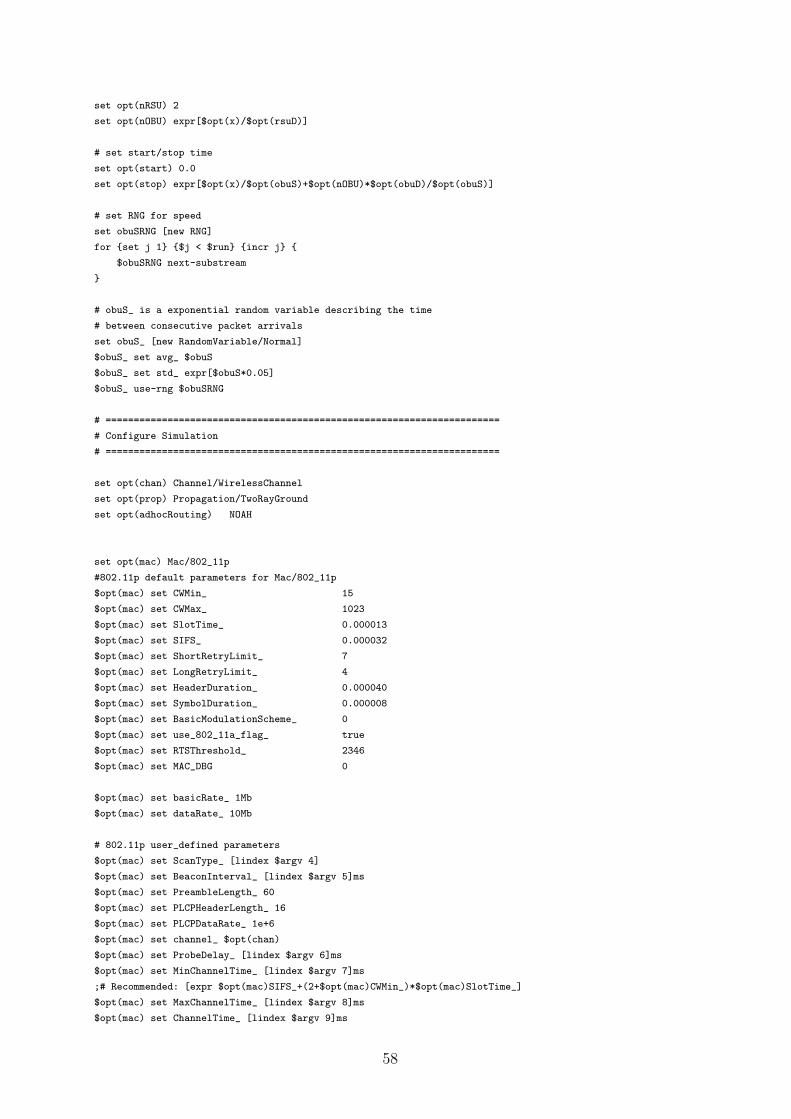
set opt(nRSU) 2
set opt(nOBU) expr[$opt(x)/$opt(rsuD)]
# set start/stop time
set opt(start) 0.0
set opt(stop) expr[$opt(x)/$opt(obuS)+$opt(nOBU)*$opt(obuD)/$opt(obuS)]
# set RNG for speed
set obuSRNG [new RNG]
for {set j 1} {$j < $run} {incr j} {
$obuSRNG next-substream
}
# obuS_ is a exponential random variable describing the time
# between consecutive packet arrivals
set obuS_ [new RandomVariable/Normal]
$obuS_ set avg_ $obuS
$obuS_ set std_ expr[$obuS*0.05]
$obuS_ use-rng $obuSRNG
# ======================================================================
# Configure Simulation
# ======================================================================
set opt(chan) Channel/WirelessChannel
set opt(prop) Propagation/TwoRayGround
set opt(adhocRouting) NOAH
set opt(mac) Mac/802_11p
#802.11p default parameters for Mac/802_11p
$opt(mac) set CWMin_ 15
$opt(mac) set CWMax_ 1023
$opt(mac) set SlotTime_ 0.000013
$opt(mac) set SIFS_ 0.000032
$opt(mac) set ShortRetryLimit_ 7
$opt(mac) set LongRetryLimit_ 4
$opt(mac) set HeaderDuration_ 0.000040
$opt(mac) set SymbolDuration_ 0.000008
$opt(mac) set BasicModulationScheme_ 0
$opt(mac) set use_802_11a_flag_ true
$opt(mac) set RTSThreshold_ 2346
$opt(mac) set MAC_DBG 0
$opt(mac) set basicRate_ 1Mb
$opt(mac) set dataRate_ 10Mb
# 802.11p user_defined parameters
$opt(mac) set ScanType_ [lindex $argv 4]
$opt(mac) set BeaconInterval_ [lindex $argv 5]ms
$opt(mac) set PreambleLength_ 60
$opt(mac) set PLCPHeaderLength_ 16
$opt(mac) set PLCPDataRate_ 1e+6
$opt(mac) set channel_ $opt(chan)
$opt(mac) set ProbeDelay_ [lindex $argv 6]ms
$opt(mac) set MinChannelTime_ [lindex $argv 7]ms
;# Recommended: [expr $opt(mac)SIFS_+(2+$opt(mac)CWMin_)*$opt(mac)SlotTime_]
$opt(mac) set MaxChannelTime_ [lindex $argv 8]ms
$opt(mac) set ChannelTime_ [lindex $argv 9]ms
58

$opt(mac) set bugFix_timer_ 0 ;# Bug description:
#http://www.dei.unipd.it/wdyn/?IDsezione=2435
set opt(netif) Phy/WirelessPhy/OFDM
#802.11p default parameters for Phy/WirelessPhyExt
$opt(netif) set CSThresh_ 3.162e-12 ;#-85 dBm Wireless interface sensitivity
;#(sensitivity defined in the standard)
$opt(netif) set Pt_ 0.001
$opt(netif) set freq_ 5.9e+9
$opt(netif) set noise_floor_ 1.26e-13 ;#-99 dBm for 10MHz bandwidth
$opt(netif) set L_ 1.0 ;#default radio circuit gain/loss
$opt(netif) set PowerMonitorThresh_ 6.310e-14 ;#-102dBm power monitor sensitivity
$opt(netif) set HeaderDuration_ 0.000040 ;#40 us
$opt(netif) set BasicModulationScheme_ 0
$opt(netif) set PreambleCaptureSwitch_ 1
$opt(netif) set DataCaptureSwitch_ 0
$opt(netif) set SINR_PreambleCapture_ 2.5118; ;# 4 dB
$opt(netif) set SINR_DataCapture_ 100.0; ;# 10 dB
$opt(netif) set trace_dist_ 1e6 ;# PHY trace until distance of 1km ("infinty")
$opt(netif) set PHY_DBG_ 0
$opt(netif) set fbandwidth_ 10e+6 ;# 10 MHz BW
$opt(netif) set g_ 4 ;#Ratio of CP (cyclic prefic) time over useful time
set opt(ifq) Queue/DropTail/PriQueue
set opt(ifqlen) 5 ;# max packet in interface queue
set opt(ll) LL
set opt(ant) Antenna/OmniAntenna
# unity gain, omni-directional antennas
# set up the antennas to be centered in the node and 1.5 meters above it
Antenna/OmniAntenna set X_ 0
Antenna/OmniAntenna set Y_ 0
Antenna/OmniAntenna set Z_ 1.5
Antenna/OmniAntenna set Gt_ 1.0
Antenna/OmniAntenna set Gr_ 1.0
# set trace files
set opt(tr) [lindex $argv 11]/[lindex $argv 12] ;# trace file
# =====================================================================
# Other default settings
# =====================================================================
LL set mindelay_ 50us
LL set delay_ 25us
LL set bandwidth_ 0 ;# not used
Agent/Null set sport_ 0
Agent/Null set dport_ 0
Agent/CBR set sport_ 0
Agent/CBR set dport_ 0
59
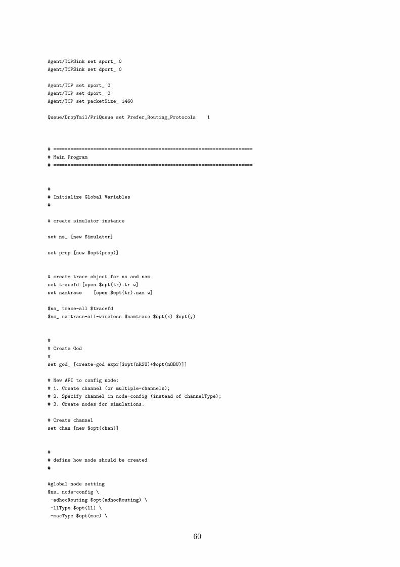
Agent/TCPSink set sport_ 0
Agent/TCPSink set dport_ 0
Agent/TCP set sport_ 0
Agent/TCP set dport_ 0
Agent/TCP set packetSize_ 1460
Queue/DropTail/PriQueue set Prefer_Routing_Protocols 1
# ======================================================================
# Main Program
# ======================================================================
#
# Initialize Global Variables
#
# create simulator instance
set ns_ [new Simulator]
set prop [new $opt(prop)]
# create trace object for ns and nam
set tracefd [open $opt(tr).tr w]
set namtrace [open $opt(tr).nam w]
$ns_ trace-all $tracefd
$ns_ namtrace-all-wireless $namtrace $opt(x) $opt(y)
#
# Create God
#
set god_ [create-god expr[$opt(nRSU)+$opt(nOBU)]]
# New API to config node:
# 1. Create channel (or multiple-channels);
# 2. Specify channel in node-config (instead of channelType);
# 3. Create nodes for simulations.
# Create channel
set chan [new $opt(chan)]
#
# define how node should be created
#
#global node setting
$ns_ node-config \
-adhocRouting $opt(adhocRouting) \
-llType $opt(ll) \
-macType $opt(mac) \
60

-ifqType $opt(ifq) \
-ifqLen $opt(ifqlen) \
-antType $opt(ant) \
-propInstance $prop \
-phyType $opt(netif) \
-channel $chan \
-topoInstance $topo \
-agentTrace ON \
-routerTrace ON \
-macTrace OFF \
-movementTrace OFF
#
# Create the specified number of nodes
#
# create Wired Node
set wnode [$ns_ node]
$wnode random-motion 0
# create RSUs
for {set i 0} {$i < $opt(nRSU)] } {incr i} {
set rsu_($i) [$ns_ node]
$rsu_($i) random-motion 0
}
# create OBUs
for {set i 0} {$i < expr[$opt(nOBU)] } {incr i} {
set obu_($i) [$ns_ node]
$obu_($i) random-motion 0
}
#
# mobility
#
$wnode set X_ expr[$opt(x)/2]
$wnode set Y_ 350.0
$wnode set Z_ 0.00
$rsu_(0) set X_ expr[($opt(x)-$opt(rsuD))/2]
$rsu_(0) set Y_ 250.0
$rsu_(0) set Z_ 0.00
$rsu_(1) set X_ expr[($opt(x)+$opt(rsuD))/2]
$rsu_(1) set Y_ 250.0
$rsu_(1) set Z_ 0.00
for {set i 0} {$i < $opt(nRSU) } {incr i} {
$obu_($i) set X_ 0.00
$obu_($i) set Y_ 250.0
$obu_($i) set Z_ 0.00
}
#
# Create the connections between the OBUs [$opt(nOBU)] and the server
#
61

for {set i 1} {$i < $opt(nOBU) } {incr i} {
set tcp($i) [new Agent/TCP]
$ns_ attach-agent $node_(0) $tcp($i)
set g($i) [new Application/Traffic/CBR]
$g($i) attach-agent $tcp($i)
$g($i) set packetSize_ 536
$g($i) set rate 1Mb
set sink($i) [new Agent/TCPSink]
$ns_ attach-agent $node_($i) $sink($i)
$ns_ connect $tcp($i) $sink($i)
}
# OBUs movement
for {set i 0} {$i < expr[$opt(nOBU)] } {incr i} {
set obu_start_time [$i*$opt(obuD)/$opt(obuS)]
set rd_obuS_ expr[$obuS_ value]
$ns_ at $obu_start_time \
"$obu_($i) setdest $opt(x) 250.00 $rd_obuS_"
$ns_ at $obu_start_time "$g($i) start"
$ns_ at expr[$obu_start_time+$opt(x)/$rd_obuS_] "$g($i) stop"
}
$ns_ initial_node_pos $wnode 150
for {set i 0} {$i < $opt(nRSU) } {incr i} {
$ns_ initial_node_pos $rsu_($i) 100
}
for {set i 0} {$i < $opt(nOBU) } {incr i} {
$ns_ initial_node_pos $obu_($i) 20
}
#
# Tell nodes when the simulation ends
#
$ns_ at $opt(stop).1 "$wnode reset";
for {set i 0} {$i < $opt(nRSU) } {incr i} {
$ns_ at $opt(stop).1 "$rsu_($i) reset";
}
for {set i 0} {$i < $opt(nOBU) } {incr i} {
$ns_ at $opt(stop).1 "$obu_($i) reset";
}
$ns_ at $opt(stop).001 "finish"
#Define ’finish’ procedure
proc finish {} {
global ns_ tracefd namtrace opt(nam)
$ns_ flush-trace
close $tracefd
close $namtrace
puts "NS EXITING..."
$ns_ halt
}
puts "Starting Simulation..."
$ns_ run
62

B.2 With Mobile IP
# simulation of a wired-cum-wireless topology running without mobileIP
if { $argc != 12 } {
puts "The $argv0 script requires eleven values to be inputed."
puts "ns $argv0 <rsuD> <obuS> <obuD> <ScanType> <BeaconInterval> \
<ProbeDelay> <MinChannelTime> <MaxChannelTime> \
<ChannelTime> <iteration> <trace_path> <trace_file>".
puts "Please try again."
exit
}
# ======================================================================
# Define options
# ======================================================================
# set run number
set run [lindex $argv 10]
# set layout and mobility patterns
set opt(rsuD) [lindex $argv 1] ;# distance between RSUs (m)
set opt(obuS) [lindex $argv 2] ;# average vehicle speed (m/s)
set opt(obuD) [lindex $argv 3] ;# starting distance between vehicles (m)
;# recommended value ~obuS/4 (safety braking distance)
# set floor size
set opt(x) expr[$opt(rsuD)+2*1200] \
;#distance required to prevent having signal at the OBUs starting point
set opt(y) 500
# define topology
set topo [new Topography]
$topo load_flatgrid $opt(x) $opt(y)
# number of nodes
set opt(nRSU) 2
set opt(nOBU) expr[$opt(x)/$opt(rsuD)]
# set start/stop time
set opt(start) 0.0
set opt(stop) expr[$opt(x)/$opt(obuS)+$opt(nOBU)*$opt(obuD)/$opt(obuS)]
# set RNG for speed
set obuSRNG [new RNG]
for {set j 1} {$j < $run} {incr j} {
$obuSRNG next-substream
}
# obuS_ is a exponential random variable describing the time
# between consecutive packet arrivals
set obuS_ [new RandomVariable/Normal]
$obuS_ set avg_ $obuS
$obuS_ set std_ expr[$obuS*0.05]
$obuS_ use-rng $obuSRNG
# ======================================================================
63
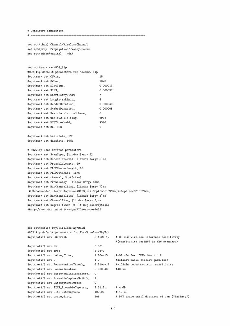
# Configure Simulation
# ======================================================================
set opt(chan) Channel/WirelessChannel
set opt(prop) Propagation/TwoRayGround
set opt(adhocRouting) NOAH
set opt(mac) Mac/802_11p
#802.11p default parameters for Mac/802_11p
$opt(mac) set CWMin_ 15
$opt(mac) set CWMax_ 1023
$opt(mac) set SlotTime_ 0.000013
$opt(mac) set SIFS_ 0.000032
$opt(mac) set ShortRetryLimit_ 7
$opt(mac) set LongRetryLimit_ 4
$opt(mac) set HeaderDuration_ 0.000040
$opt(mac) set SymbolDuration_ 0.000008
$opt(mac) set BasicModulationScheme_ 0
$opt(mac) set use_802_11a_flag_ true
$opt(mac) set RTSThreshold_ 2346
$opt(mac) set MAC_DBG 0
$opt(mac) set basicRate_ 1Mb
$opt(mac) set dataRate_ 10Mb
# 802.11p user_defined parameters
$opt(mac) set ScanType_ [lindex $argv 4]
$opt(mac) set BeaconInterval_ [lindex $argv 5]ms
$opt(mac) set PreambleLength_ 60
$opt(mac) set PLCPHeaderLength_ 16
$opt(mac) set PLCPDataRate_ 1e+6
$opt(mac) set channel_ $opt(chan)
$opt(mac) set ProbeDelay_ [lindex $argv 6]ms
$opt(mac) set MinChannelTime_ [lindex $argv 7]ms
;# Recommended: [expr $opt(mac)SIFS_+(2+$opt(mac)CWMin_)*$opt(mac)SlotTime_]
$opt(mac) set MaxChannelTime_ [lindex $argv 8]ms
$opt(mac) set ChannelTime_ [lindex $argv 9]ms
$opt(mac) set bugFix_timer_ 0 ;# Bug description:
#http://www.dei.unipd.it/wdyn/?IDsezione=2435
set opt(netif) Phy/WirelessPhy/OFDM
#802.11p default parameters for Phy/WirelessPhyExt
$opt(netif) set CSThresh_ 3.162e-12 ;#-85 dBm Wireless interface sensitivity
;#(sensitivity defined in the standard)
$opt(netif) set Pt_ 0.001
$opt(netif) set freq_ 5.9e+9
$opt(netif) set noise_floor_ 1.26e-13 ;#-99 dBm for 10MHz bandwidth
$opt(netif) set L_ 1.0 ;#default radio circuit gain/loss
$opt(netif) set PowerMonitorThresh_ 6.310e-14 ;#-102dBm power monitor sensitivity
$opt(netif) set HeaderDuration_ 0.000040 ;#40 us
$opt(netif) set BasicModulationScheme_ 0
$opt(netif) set PreambleCaptureSwitch_ 1
$opt(netif) set DataCaptureSwitch_ 0
$opt(netif) set SINR_PreambleCapture_ 2.5118; ;# 4 dB
$opt(netif) set SINR_DataCapture_ 100.0; ;# 10 dB
$opt(netif) set trace_dist_ 1e6 ;# PHY trace until distance of 1km ("infinty")
64
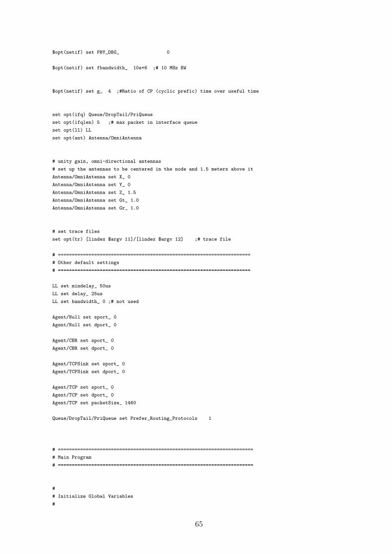
$opt(netif) set PHY_DBG_ 0
$opt(netif) set fbandwidth_ 10e+6 ;# 10 MHz BW
$opt(netif) set g_ 4 ;#Ratio of CP (cyclic prefic) time over useful time
set opt(ifq) Queue/DropTail/PriQueue
set opt(ifqlen) 5 ;# max packet in interface queue
set opt(ll) LL
set opt(ant) Antenna/OmniAntenna
# unity gain, omni-directional antennas
# set up the antennas to be centered in the node and 1.5 meters above it
Antenna/OmniAntenna set X_ 0
Antenna/OmniAntenna set Y_ 0
Antenna/OmniAntenna set Z_ 1.5
Antenna/OmniAntenna set Gt_ 1.0
Antenna/OmniAntenna set Gr_ 1.0
# set trace files
set opt(tr) [lindex $argv 11]/[lindex $argv 12] ;# trace file
# =====================================================================
# Other default settings
# =====================================================================
LL set mindelay_ 50us
LL set delay_ 25us
LL set bandwidth_ 0 ;# not used
Agent/Null set sport_ 0
Agent/Null set dport_ 0
Agent/CBR set sport_ 0
Agent/CBR set dport_ 0
Agent/TCPSink set sport_ 0
Agent/TCPSink set dport_ 0
Agent/TCP set sport_ 0
Agent/TCP set dport_ 0
Agent/TCP set packetSize_ 1460
Queue/DropTail/PriQueue set Prefer_Routing_Protocols 1
# ======================================================================
# Main Program
# ======================================================================
#
# Initialize Global Variables
#
65

# create simulator instance
set ns_ [new Simulator]
set prop [new $opt(prop)]
# set up for hierarchical routing
$ns_ node-config -addressType hierarchical
AddrParams set domain_num_ 3 ;# number of domains
lappend cluster_num 1 1 1 ;# number of clusters in each domain
AddrParams set cluster_num_ $cluster_num
lappend eilastlevel 1 2 $opt(nOBU) ;# number of nodes in each cluster
AddrParams set nodes_num_ $eilastlevel ;# of each domain
# create trace object for ns and nam
set tracefd [open $opt(tr).tr w]
set namtrace [open $opt(tr).nam w]
$ns_ trace-all $tracefd
$ns_ namtrace-all-wireless $namtrace $opt(x) $opt(y)
#
# Create God
#
set god_ [create-god expr[$opt(nRSU)+$opt(nOBU)]]
# New API to config node:
# 1. Create channel (or multiple-channels);
# 2. Specify channel in node-config (instead of channelType);
# 3. Create nodes for simulations.
# Create channel
set chan [new $opt(chan)]
#
# define how node should be created
#
#global node setting
$ns_ node-config \
-mobileIP ON \
-adhocRouting $opt(adhocRouting) \
-llType $opt(ll) \
-macType $opt(mac) \
-ifqType $opt(ifq) \
-ifqLen $opt(ifqlen) \
-antType $opt(ant) \
-propInstance $prop \
-phyType $opt(netif) \
-channel $chan \
-topoInstance $topo \
-agentTrace ON \
-routerTrace ON \
-macTrace OFF \
-movementTrace OFF
#
# Create the specified number of nodes
66
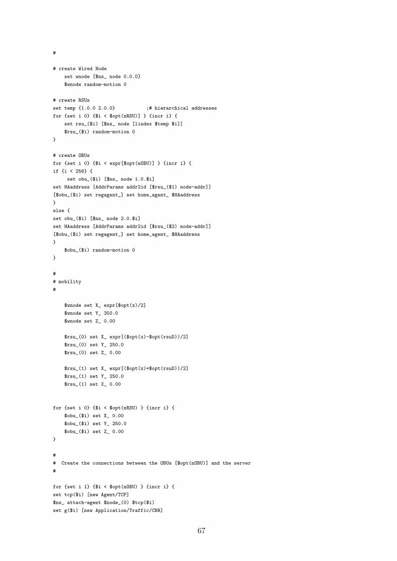
#
# create Wired Node
set wnode [$ns_ node 0.0.0]
$wnode random-motion 0
# create RSUs
set temp {1.0.0 2.0.0} ;# hierarchical addresses
for {set i 0} {$i < $opt(nRSU)] } {incr i} {
set rsu_($i) [$ns_ node [lindex $temp $i]]
$rsu_($i) random-motion 0
}
# create OBUs
for {set i 0} {$i < expr[$opt(nOBU)] } {incr i} {
if {i < 256} {
set obu_($i) [$ns_ node 1.0.$i]
set HAaddress [AddrParams addr2id [$rsu_($1) node-addr]]
[$obu_($i) set regagent_] set home_agent_ $HAaddress
}
else {
set obu_($i) [$ns_ node 2.0.$i]
set HAaddress [AddrParams addr2id [$rsu_($2) node-addr]]
[$obu_($i) set regagent_] set home_agent_ $HAaddress
}
$obu_($i) random-motion 0
}
#
# mobility
#
$wnode set X_ expr[$opt(x)/2]
$wnode set Y_ 350.0
$wnode set Z_ 0.00
$rsu_(0) set X_ expr[($opt(x)-$opt(rsuD))/2]
$rsu_(0) set Y_ 250.0
$rsu_(0) set Z_ 0.00
$rsu_(1) set X_ expr[($opt(x)+$opt(rsuD))/2]
$rsu_(1) set Y_ 250.0
$rsu_(1) set Z_ 0.00
for {set i 0} {$i < $opt(nRSU) } {incr i} {
$obu_($i) set X_ 0.00
$obu_($i) set Y_ 250.0
$obu_($i) set Z_ 0.00
}
#
# Create the connections between the OBUs [$opt(nOBU)] and the server
#
for {set i 1} {$i < $opt(nOBU) } {incr i} {
set tcp($i) [new Agent/TCP]
$ns_ attach-agent $node_(0) $tcp($i)
set g($i) [new Application/Traffic/CBR]
67

$g($i) attach-agent $tcp($i)
$g($i) set packetSize_ 92
$g($i) set rate 1Mb
set sink($i) [new Agent/TCPSink]
$ns_ attach-agent $node_($i) $sink($i)
$ns_ connect $tcp($i) $sink($i)
}
# OBUs movement
for {set i 0} {$i < expr[$opt(nOBU)] } {incr i} {
set obu_start_time [$i*$opt(obuD)/$opt(obuS)]
set rd_obuS_ expr[$obuS_ value]
$ns_ at $obu_start_time \
"$obu_($i) setdest $opt(x) 250.00 $rd_obuS_"
$ns_ at $obu_start_time "$g($i) start"
$ns_ at expr[$obu_start_time+$opt(x)/$rd_obuS_] "$g($i) stop"
}
$ns_ initial_node_pos $wnode 150
for {set i 0} {$i < $opt(nRSU) } {incr i} {
$ns_ initial_node_pos $rsu_($i) 100
}
for {set i 0} {$i < $opt(nOBU) } {incr i} {
$ns_ initial_node_pos $obu_($i) 20
}
#
# Tell nodes when the simulation ends
#
$ns_ at $opt(stop).1 "$wnode reset";
for {set i 0} {$i < $opt(nRSU) } {incr i} {
$ns_ at $opt(stop).1 "$rsu_($i) reset";
}
for {set i 0} {$i < $opt(nOBU) } {incr i} {
$ns_ at $opt(stop).1 "$obu_($i) reset";
}
$ns_ at $opt(stop).001 "finish"
#Define ’finish’ procedure
proc finish {} {
global ns_ tracefd namtrace opt(nam)
$ns_ flush-trace
close $tracefd
close $namtrace
puts "NS EXITING..."
$ns_ halt
}
puts "Starting Simulation..."
$ns_ run
68
Appendix C
Batched Simulations and Analysis
C.1 Bash Shell Script for Batched Simulations
By means of this script researchers will be able to perform valid simulations for their
research once the simulation environment is properly configured as shown in app. A.
The aforementioned script consists of a series of menus which will allow the config-
uration of the scripts available at App. B, already explained in Chapter 4.
C.1.1 Considerations
Scripting language
Of the available choices —high level programming as Java, C, etc. or scripting lan-
guage as perl, python, bash. . . — high level programming was not considered due to
the potential portability issues, either in terms of compilation, libraries available in the
operating system (OS) or compatibility of specific instructions such as exec, required
for our simulation. Therefore, the choice was batch scripting.
Among the scripting languages, bash[42][43][44] was chosen as it is already included
on the vast majority of OS’s where ns-2 can be installed, including all Unix-based OS’s1
—being in most of them the default shell— and is available for installation in Cyg-
win. The use of shell scripting avoids potential missing library issues of other scripting
languages such as python or perl.
1Unix-based OS’s include all the Linux distributions —Ubuntu, Red Hat’s Fedora. . . — and MacOSoperating systems
69

Bash is very convenient as it is easy to understand and extend. In this research it
is a desirable feature as foreseeable common operations such as adopting the system for
particular requirements should be easy to implement.
Number of simulations
To prevent the exponentially growing number of simulations performed, not all the
possible permutations for all the values in each interval defined will be implemented,
as the number of simulations in the event that there are intervals defined would be
Iterations × ∏∀intervals definedNumber of steps, leading to an extremely large amount
of simulations depending on the configuration.
For that reason the choice of one value in the interval has to be made, and that will be
the value used for batched simulations where other parameters are being swept. This will
reduce a the amount of simulations to Iterations× ∑∀intervals definedNumber of steps,
decreasing the number of runs required to obtain the results of simulations which in
most situations would not provide valuable results.
The only exception for this is ScanType , which can only be set up to ACTIVE,
PASSIVE or BOTH, which implies a ×2 factor to the number of runs in case it is demanded
to perform simulations using both active and passive scanning methods.
70

C.1.2 Interface
Main Menu
# # # # # # # # # # # # # # # #
# Parameter Configuration #
# # # # # # # # # # # # # # # #
#
# Scanning Type_ PASSIVE.
#
# BeaconInterval_ 300 ms.
#
# ProbeDelay_ 10 ms.
#
# MinChannelTime_ 20 ms.
#
# MaxChannelTime_ 50 ms.
#
# ChannelTime_ 300 ms.
#
# Distance between RSUs:
# rsuD_ 2000 m.
#
# Average OBUs Speed:
# obuS_ 30 m/s.
#
# Start Inter-OBU Distance:
# obuD_ 80 m.
#
# Number of iterations: 10.
#
# # # # # # # # # # # # # # # #
1) Modify 3) Save_and_Execute
2) Save_script 4) Exit
#?
Modifying Parameters
What do you want to change?
1) Scanning 5) Max_Channel_Time 9) All
2) Beacon_Interval 6) Channel_Time 10) None
3) Probe_Delay 7) Mobility
4) Min_Channel_Time 8) Iterations
#? 2
# # # # # # # # # # # # # # # #
# Current Configuration #
# # # # # # # # # # # # # # # #
#
# BeaconInterval_ 300 ms.
#
1) Unique_Value
2) Interval
3) Do_not_modify
#? 2
Introduce the starting value in ms:
100
Introduce the ending value in ms:
300
In order to prevent excessive simulations when another variable
is being swept this variable should take a unique value.
Introduce now a middle value for BeaconInterval_ in ms:
200
Choose the steps by introducing the number of steps or the gap between simulations:
1) Number_of_steps
71

2) Gap_between_simulations
#? 2
Introduce the gap between steps in ms:
20
# # # # # # # # # # # # # # # #
# Parameter Configuration #
# # # # # # # # # # # # # # # #
#
# Scanning Type_ PASSIVE.
#
# BeaconInterval_ from 100 to 300 ms in steps of 20 ms.
# (when the variable is not swept: 200 ms)
#
# ProbeDelay_ 10 ms.
#
# MinChannelTime_ 20 ms.
#
# MaxChannelTime_ 50 ms.
#
# ChannelTime_ 300 ms.
#
# Distance between RSUs:
# rsuD_ 2000 m.
#
# Average OBUs Speed:
# obuS_ 30 m/s.
#
# Start Inter-OBU Distance:
# obuD_ 80 m.
#
# Number of iterations: 10.
#
# # # # # # # # # # # # # # # #
1) Modify 3) Save_and_Execute
2) Save_script 4) Exit
#?
Generating the bashed simulation script
and the analysis script
Input the name for the batch script file and results folder:
(Please do not use spaces)
safe_output
WARNING! If there is already a file with the name "safe_output.sh" will be overwritten!!
WARNING! If there is already a folder with the name "safe_output_traces" will be overwritten!!
1) Return
2) Change_name
3) OK!
#? 3
Select the simulation script:
1) Without_Mobile_IP
2) With_Mobile_IP
#? 1
C.1.3 Output
The main output of the script are:
72

• Simulation script: Another bash script prepared to execute all the requested sim-
ulations and save the traces in the simulationName traces folder. If the option
chosen was not only Save but Save and Execute it will also execute this script.
• Analysis script: Again this is a bash script output ready to, by means of the awk
scripts described in section C.2, calculate all the statistics for each individual trace
file, average the different run simulations and create a file with the best configu-
ration parameters for each different performance indicator described in 4.2.3
C.1.4 Expanding the framework
The design of the batched simulation script has taken into account the expansion by
adding new ns .tcl scripts in the tcl folder. To add new simulation files there are a
few requirements:
• the file has to have tcl extension. Any file with tcl extension in the tcl folder
will be considered a valid ns script.
• the file name must not contain spaces or special characters.
• the file name has to be descriptive, as it will be the option available during the
script execution.
• the parameter setup has to be consistent with the following:
– rsuD is [lindex $argv 1]
– obuS is [lindex $argv 2]
– obuD is [lindex $argv 3]
– ScanType is [lindex $argv 4]
– BeaconInterval is [lindex $argv 5]
– ProbeDelay is [lindex $argv 6]
– MinChannelTime is [lindex $argv 7]
– MaxChannelTime is [lindex $argv 8]
– ChannelTime is [lindex $argv 9]
– iteration is [lindex $argv 10]
– trace file name is [lindex $argv 11]
73

C.1.5 Code
#!/bin/bash
# Bash Shell Script for Batched Simulations
# by Pablo Urmeneta (c) 2010
# standard values
ScanType_=PASSIVE
BeaconInterval_=300
ProbeDelay_=10
MinChannelTime_=20
MaxChannelTime_=50
ChannelTime_=300
rsuD_=2000
obuS_=30
obuD_=80
Iterations_=10
route=$route
ns_script=$ns_script
BeaconInterval_start=$BeaconInterval_start
BeaconInterval_end=$BeaconInterval_end
BeaconInterval_step=0
ProbeDelay_start=$ProbeDelay_start
ProbeDelay_end=$ProbeDelay_end
ProbeDelay_step=0
MinChannelTime_start=$MinChannelTime_start
MinChannelTime_end=$MinChannelTime_end
MinChannelTime_step=0
MaxChannelTime_start=$MaxChannelTime_start
MaxChannelTime_end=$MaxChannelTime_end
MaxChannelTime_step=0
ChannelTime_start=$ChannelTime_start
ChannelTime_end=$ChannelTime_end
ChannelTime_step=0
rsuD_start=$rsuD_start
rsuD_end=$rsuD_end
rsuD_step=0
robuS_start=$obuS_start
obuS_end=$obuS_end
obuS_step=0
obuD_start=$obuS_start
obuD_end=$obuD_end
obuD_step=0
all=0
execute=0
sim=$sim
save_status=1
end_sim=0
stats=$stats
end_stats=0
#
## Value Printing Functions
#
function p_scan () {
echo \# Scanning Type_ ${ScanType_}.
echo \#
}
function p_multi () {
cond=$(eval "echo \${$2step}")
if [ "$cond" = "0" ]; then
echo \# $2 ${!2} $3.
else
echo -n \# $2 from $(eval "echo \${$2start}") to $(eval "echo \${$2end}") $3
echo in steps of $(eval "echo \${$2step}") $3.
echo \# \(when the variable is not swept: $(eval "echo \${$2}") $3\)
fi
echo \#
74

}
function p_iter () {
echo \# Number of iterations: ${Iterations_}.
echo \#
}
function p_mob () {
echo \# Distance between RSUs:
p_multi mob_rsuD rsuD_ m
echo \# Average OBUs Speed:
p_multi mob_obuS obuS_ m/s
echo \# Start Inter-OBU Distance:
p_multi mob_obuD obuD_ m
}
function p_ () {
if [ "$1" = "beacon" ]; then
p_multi beacon BeaconInterval_ ms
elif [ "$1" = "probe" ]; then
p_multi probe ProbeDelay_ ms
elif [ "$1" = "minct" ]; then
p_multi minct MinChannelTime_ ms
elif [ "$1" = "maxct" ]; then
p_multi maxct MaxChannelTime_ ms
elif [ "$1" = "ct" ]; then
p_multi ct ChannelTime_ ms
elif [ "$1" = "mob_rsuD" ]; then
p_multi mob_rsuD rsuD_ m
elif [ "$1" = "mob_obuS" ]; then
p_multi mob_obuS obuS_ m/s
elif [ "$1" = "mob_obuD" ]; then
p_multi mob_obuD obuD_ m
else
p_$1
fi
}
function p_2 () {
clear
echo \# \# \# \# \# \# \# \# \# \# \# \# \# \# \# \#
echo \# \ \ \ Current Configuration \ \ \ \#
echo \# \# \# \# \# \# \# \# \# \# \# \# \# \# \# \#
echo \#
p_ $1
echo
}
function p_all () {
echo \# \# \# \# \# \# \# \# \# \# \# \# \# \# \# \#
echo \# \ \ Parameter Configuration \ \ \#
echo \# \# \# \# \# \# \# \# \# \# \# \# \# \# \# \#
echo \#
p_ scan
p_ beacon
p_ probe
p_ minct
p_ maxct
p_ ct
p_ mob
p_ iter
echo \# \# \# \# \# \# \# \# \# \# \# \# \# \# \# \#
echo
}
function parameters () {
clear
p_all
choice
}
#
75

## Menu
#
function choice () {
OPTIONS="Modify Save_script Save_and_Execute Exit"
select opt in $OPTIONS; do
if [ "$opt" = "Modify" ]; then
change_menu
elif [ "$opt" = "Save_script" ]; then
save_warning
elif [ "$opt" = "Save_and_Execute" ]; then
execute=1
save_warning
elif [ "$opt" = "Exit" ]; then
end
else
echo bad option: introduce option again
fi
done
}
function change_menu () {
echo What do you want to change?
OPTIONS="Scanning Beacon_Interval Probe_Delay\
Min_Channel_Time Max_Channel_Time Channel_Time\
Mobility Iterations All None"
select opt in $OPTIONS; do
if [ "$opt" = "Scanning" ]; then
modify scan
elif [ "$opt" = "Beacon_Interval" ]; then
modify beacon BeaconInterval_ ms
elif [ "$opt" = "Probe_Delay" ]; then
modify probe ProbeDelay_ ms
elif [ "$opt" = "Min_Channel_Time" ]; then
modify minct MinChannelTime_ ms
elif [ "$opt" = "Max_Channel_Time" ]; then
modify maxct MaxChannelTime_ ms
elif [ "$opt" = "Channel_Time" ]; then
modify ct ChannelTime_ ms
elif [ "$opt" = "Mobility" ]; then
modify mob
elif [ "$opt" = "Iterations" ]; then
modify iter
elif [ "$opt" = "All" ]; then
all=1
modify scan
elif [ "$opt" = "None" ]; then
parameters
else
echo bad option: introduce option again
fi
done
}
#
## Step-by-step Value Modification
#
function modify () {
p_2 $1
if [[ "$1" = "scan" ]]; then
modify_scan
elif [ "$1" = "iter" ]; then
modify_iter
elif [ "$1" = "mob" ]; then
modify_mob
else
OPTIONS="Unique_Value Interval Do_not_modify"
select opt in $OPTIONS; do
if [ "$opt" = "Unique_Value" ]; then
echo Introduce the value for $2 in $3:
read $2
eval $2step="0"
76

modify_next $1
elif [ "$opt" = "Interval" ]; then
modify_int $1 $2 $3
elif [ "$opt" = "Do_not_modify" ]; then
echo $2 = ${!2}
modify_next $1
else
echo bad option: introduce option again
fi
done
fi
}
function modify_int () {
echo Introduce the starting value in $3:
read $2start
eval t_start=$(eval "echo \${$2start}")
echo Introduce the ending value in $3:
read $2end
eval t_end=$(eval "echo \${$2end}")
#check if end is bigger than start
cond=$(echo "$t_start>=$t_end" | bc)
if [ "$cond" -eq "1" ]; then
echo Error: $2end must be bigger than $2start
modify_int $1 $2 $3
else
echo In order to prevent excessive simulations when another variable
echo is being swept this variable should take a unique value.
cond="0"
while [ "$cond" -ne "1" ]; do
echo Introduce now a middle value for $2 in $3:
read $2
t_=$(eval "echo \${$2}")
cond=$(echo "($t_end >= $t_ && $t_ >= $t_start)" | bc)
if [ "$cond" -ne "1" ]; then
echo The value has to be in the previously defined interval\!
fi
done
echo Choose the steps by introducing the number of steps or the gap between simulations:
OPTIONS="Number_of_steps Gap_between_simulations"
select opt in $OPTIONS; do
if [ "$opt" = "Number_of_steps" ]; then
cond=0
while [[ "$cond" -ne "1" ]]; do
echo Introduce the number of steps:
read temp
cond=$(echo "($temp >= 1)" | bc)
if [ "$cond" -ne "1" ]; then
echo The value has to be greater or equal than \"1\"\!
fi
done
eval $2step=$(echo "scale=6; ( $t_end-$t_start )/$temp;" | bc)
modify_next $1
elif [ "$opt" = "Gap_between_simulations" ]; then
echo Introduce the gap between steps in $3:
read $2step
eval t_step=$(eval "echo \${$2step}")
cond=$(echo "( $t_end-$t_start )<$t_step" | bc)
while [[ $cond -eq "1" ]]; do
echo The gap is too big. Reintroduce gap between steps:
read $2step
cond=$(echo "( $t_end-$t_start )<$t_step" | bc)
done
modify_next $1
else
echo bad option: introduce option again
fi
done
fi
}
function modify_next () {
77

if [ "$all" = 1 ]; then
if [[ "$1" = "scan" ]]; then
modify beacon BeaconInterval_ ms
elif [[ "$1" = "beacon" ]]; then
modify probe ProbeDelay_ ms
elif [[ "$1" = "probe" ]]; then
modify minct MinChannelTime_ ms
elif [[ "$1" = "minct" ]]; then
modify maxct MaxChannelTime_ ms
elif [[ "$1" = "maxct" ]]; then
modify ct ChannelTime_ ms
elif [[ "$1" = "ct" ]]; then
modify mob
elif [[ "$1" = "mob" ]]; then
modify iter
elif [[ "$1" = "iter" ]]; then
parameters
else
modify mob
fi
elif [ "$1" = "mob_rsuD" ] || [ "$1" = "mob_obuS" ] || [ "$1" = "mob_obuD" ]; then
modify mob
else
parameters
fi
}
function modify_scan () {
OPTIONS="ACTIVE PASSIVE BOTH Do_not_modify"
select opt in $OPTIONS; do
if [ "$opt" = "ACTIVE" ]; then
ScanType_=ACTIVE
elif [ "$opt" = "PASSIVE" ]; then
ScanType_=PASSIVE
elif [ "$opt" = "BOTH" ]; then
ScanType_=BOTH
elif [ "$opt" = "Do_not_modify"]; then
echo ScanType_ = ${ScanType_}
else
echo bad option: introduce option again
fi
modify_next scan
done
}
function modify_mob () {
OPTIONS="Modify_RSU_Distance Modify_OBU_Average_Speed Modify_OBU_Average_Distance Done"
select opt in $OPTIONS; do
if [ "$opt" = "Modify_RSU_Distance" ]; then
modify mob_rsuD rsuD_ m
elif [ "$opt" = "Modify_OBU_Average_Speed" ]; then
modify mob_obuS obuS_ m/s
elif [ "$opt" = "Modify_OBU_Average_Distance" ]; then
modify mob_obuD obuD_ m
elif [ "$opt" = "Done" ]; then
echo rsuD_ = ${rsuD_}
echo obuS_ = ${obuS_}
echo obuD_ = ${obuD_}
modify_next mob
else
echo bad option: introduce option again
fi
done
}
function modify_iter () {
p_2 iter
OPTIONS="Modify Do_not_modify"
select opt in $OPTIONS; do
78

if [ "$opt" = "Modify" ]; then
echo Introduce the number of iterations:
read Iterations_
elif [ "$opt" = "Do_not_modify" ]; then
echo Iterations_ = ${Iterations_}
else
echo bad option: introduce option again
fi
if [ "$all" = 1 ]; then
all=0
echo All parameters set up!
fi
modify_next iter
done
}
#
## Saving and executing
#
function save_warning () {
echo Input the name for the batch script file and results folder:
echo \(Please do not use spaces\)
read temp
echo WARNING\! If there is already a file with the name \"${temp}.sh\" will be overwritten\!\!
# echo WARNING\! If there is already a folder with the name \"${temp}\" it will be overwritten\!\!
echo WARNING\! If there is already a folder with the name \"${temp}\_traces\" will be overwritten\!\!
OPTIONS="Return Change_name OK!"
select opt in $OPTIONS; do
if [ "$opt" = "Return" ]; then
execute=0
parameters
elif [ "$opt" = "Change_name" ]; then
save_warning
elif [ "$opt" = "OK!" ]; then
sim=$temp
script_select
else
echo bad option: introduce option again
fi
parameters
done
}
function script_select () {
echo Select the simulation script:
OPTIONS=$(ls tcl/*.tcl | awk ’{sub(/tcl\//, "", $0); sub(/.tcl/,"",$0); printf ("%s ",$0)}’)
select opt in $OPTIONS; do
ns_script="opt"
stats_choice
done
}
function save () {
echo \#!/bin/bash > $sim.sh
chmod 755 ${sim}.sh
echo "$(date "+# DATE: %Y-%m-%d%n# TIME: %H:%M:%S%n")" >> $sim.sh
p_all >> $sim.sh
echo
echo rm -rd $sim >> $sim.sh
echo mkdir $sim\_traces >> $sim.sh
route=$sim\_traces
while [[ "$end_save" -ge "1" ]]; do
script_builder
done
if [[ -z "$stats" ]]; then
echo awk -f ./awk/parameter_choice.awk ./$stats.txt >> ./$stats_choice.txt
echo "echo \# Calculating statistics . . ." >> $sim.sh
echo ./${stats}.sh >> $sim.sh
echo "echo \# Statistics calculated\!" >> $sim.sh
echo "echo \# Statistics can be found at $stats.txt and the $stats folder"
79

fi
end_sim="1"
if [ "$execute" = "1" ]; then
execute=0
echo executing . . .
echo
./${sim}.sh
echo
end_sim="1"
echo Batched execution finished\!
if [[ -z "$stats" ]]; then
end_stats="1"
fi
OPTIONS="New_Simulation Exit"
select opt in $OPTIONS; do
if [ "$opt" = "New_Simulation" ]; then
unset sim
end_sim="0"
unset stats
end_stats="0"
parameters
elif [ "$opt" = "Exit" ]; then
end
else
echo bad option: introduce option again
fi
done
else
parameters
fi
}
function script_builder () {
if [[ "$ScanType_" = "BOTH" ]]; then
ScanType_=ACTIVE
mkdir $sim\_traces/$ScanType_ >> $sim.sh
route=$sim\_traces/$ScanType_
script_builder
ScanType_=PASSIVE
mkdir $sim\_traces/$ScanType_ >> $sim.sh
route=$sim\_traces/$ScanType_
script_builder
ScanType_=BOTH
route=$sim\_traces
exit
else
cond_beacon=$(echo "$BeaconInterval_step != 0" | bc)
(( save_status += $cond_beacon ))
cond_probe=$(echo "$ProbeDelay_step != 0" | bc)
(( save_status += $cond_probe ))
cond_minct=$(echo "$MinChannelTime_step != 0" | bc)
(( save_status += $cond_minct ))
cond_maxct=$(echo "$MaxChannelTime_step != 0" | bc)
(( save_status += $cond_maxct ))
cond_ct=$(echo "$ChannelTime_step != 0" | bc)
(( save_status += $cond_ct ))
cond_rsuD=$(echo "$rsuD_step != 0" | bc)
(( save_status += $cond_rsuD ))
cond_obuS=$(echo "$obuS_step != 0" | bc)
(( save_status += $cond_obuS ))
cond_obuD=$(echo "$obuD_step != 0" | bc)
(( save_status += $cond_obuD ))
if [[ "cond_beacon" -eq "1" ]]; then
add_script_lines "BeaconInterval_"
temp="1"
(( save_status -= "1" ))
fi
if [[ "cond_probe" -eq "1" ]]; then
add_script_lines "ProbeDelay_"
temp="1"
(( save_status -= "1" ))
80

fi
if [[ "cond_minct" -eq "1" ]]; then
add_script_lines "MinChannelTime_"
temp="1"
(( save_status -= "1" ))
fi
if [[ "cond_maxct" -eq "1" ]]; then
add_script_lines "MaxChannelTime_"
temp="1"
(( save_status -= "1" ))
fi
if [[ "cond_ct" -eq "1" ]]; then
add_script_lines "ChannelTime_"
temp="1"
(( save_status -= "1" ))
fi
if [[ "cond_rsuD" -eq "1" ]]; then
add_script_lines "rsuD_"
temp="1"
(( save_status -= "1" ))
fi
if [[ "cond_obuS" -eq "1" ]]; then
add_script_lines "obuS_"
temp="1"
(( save_status -= "1" ))
fi
if [[ "cond_obuD" -eq "1" ]]; then
add_script_lines "obuD_"
temp="1"
(( save_status -= "1" ))
fi
if [[ "$temp" -ne "1" ]]; then
add_script_lines "-1" "general"
(( save_status -= "1" ))
fi
fi
if [[ -z "$stats" ]]; then
echo "awk -f ./awk/parameter_choice.awk $stats.txt > ./$stats_choice.txt " >> $stats.sh
fi
}
function add_script_lines () {
if [[ "$1" = "-1" ]]; then
config_name=$sim_\_$ns_script\_$rsuD_\_$obuS_\_$obuD_\_$ScanType_\_$BeaconInterval_\
\_$ProbeDelay_\_$MinChannelTime_\_$MaxChannelTime_\_$ChannelTime_
for (( i=0; i < $Iterations_; i++ )); do
echo ns tcl/$ns_script.tcl $rsuD_ $obuS_ $obuD_ $ScanType_ $BeaconInterval_ $ProbeDelay_\
$MinChannelTime_ $MaxChannelTime_ $ChannelTime_ $i "$route" $config_name\_$i >> $sim.sh
if [[ -z "$stats" ]]; then
echo "echo "\# Parameters throughput delay_min delay_max delay_avg total_AGTpackets_sent\
total_AGTpackets_received total_AGTpackets_dropped pkt_delivery_ratio\
latency ponderated_latency" > ./$stats/$2.txt" >> $stats.sh
echo "echo -n "$config_name\_$i " > ./$stats/$2.txt" >> $stats.sh
echo "awk -f ./awk/performance.awk "$route"/$config_name\_$i.tr >> ./$stats/$2.txt " >> $stats.sh
fi
done
if [[ -z "$stats" ]]; then
echo "echo -n "$config_name " > ./$stats.txt" >> $stats.sh
echo "awk -f ./awk/average.awk ./$stats/$2.txt > ./$stats.txt" >> $stats.sh
fi
else
t_route=$route
echo >> $sim.sh
echo \# Starting batched simulation for $1 >> $sim.sh
echo mkdir $t_route/$1 >> $sim.sh
route=$t_route/$1
echo $route
temp=$(eval "echo \${$1}")
echo $temp
t_status=$(eval "echo \${$1start}")
t_end=$(eval "echo \${$1end}")
t_step=$(eval "echo \${$1step}")
eval $1=$t_status
81

echo check: $(eval "echo \${$1}")
cond_="1"
while [[ "$cond_" -eq "1" ]]; do
add_script_lines "-1" "$1"
t_status=$(echo "scale=5; $t_status + $t_step;" | bc)
echo >> $sim.sh
eval $1=$t_status
echo check: $(eval "echo \${$1}")
cond_=$(echo "$t_status <= $t_end" | bc)
done
eval $1=$temp
route=$t_route
fi
}
#
## Statistics
#
function stats_choice () {
echo "Do you want to calculate the statistics for the simulation?"
OPTIONS="Yes No"
select opt in $OPTIONS; do
if [ "$opt" = "Yes" ]; then
stats_warning
elif [ "$opt" = "No" ]; then
echo No statistics will be calculated.
save
else
echo bad option: introduce option again
fi
done
}
function stats_warning () {
echo Input the name for the statistics file:
echo \(Please do not use spaces\)
read temp
if [[ "$temp" = "$sim" ]]; then
echo Statistics file name can not be the same as the script name \(${sim}\)
stats_warning
fi
echo WARNING\! If there is already a file with the name \"${temp}.txt\" will be overwritten\!\!
echo WARNING\! If there is already a file with the name \"${temp}_choice.txt\" will be overwritten\!\!
echo WARNING\! If there is already a file with the name \"${temp}.sh\" will be overwritten\!\!
echo WARNING\! If there is already a folder with the name \"${temp}\" will be overwritten\!\!
OPTIONS="Do_not_save Change_name OK!"
select opt in $OPTIONS; do
if [ "$opt" = "Do_not_save" ]; then
echo Not generating statistics.
save
elif [ "$opt" = "Change_name" ]; then
stats_warning
elif [ "$opt" = "OK!" ]; then
stats=$temp
echo \#!/bin/bash > $stats.sh
chmod 755 ${stats}.sh
echo "$(date "+# DATE: %Y-%m-%d%n# TIME: %H:%M:%S%n")" >> $stats.sh
p_all >> $stats.sh
echo
echo "echo -n "\# Parameters avg_throughput avg_delay_min avg_delay_max avg_delay\
avg_total_AGTpackets_sent avg_total_AGTpackets_received avg_total_AGTpackets_dropped\
avg_pkt_delivery_ratio avg_latency avg_ponderated_latency" > $stats.txt" >> $stats.sh
echo "echo -n "\# std_dev_throughput std_dev_delay_min std_dev_delay_max std_dev_delay\
std_dev_total_AGTpackets_sent std_dev_total_AGTpackets_received std_dev_total_AGTpackets_dropped\
std_dev_pkt_delivery_ratio std_dev_latency std_dev_ponderated_latency" > $stats.txt" >> $stats.sh
echo "echo -n "\# min_throughput min_delay_min min_delay_max min_delay min_total_AGTpackets_sent\
min_total_AGTpackets_received min_total_AGTpackets_dropped min_pkt_delivery_ratio min_latency\
min_ponderated_latency" > $stats.txt" >> $stats.sh
echo "echo "\# max_throughput max_delay_min max_delay_max max_delay max_total_AGTpackets_sent\
max_total_AGTpackets_received max_total_AGTpackets_dropped max_pkt_delivery_ratio max_latency\
82

max_ponderated_latency" > $stats.txt" >> $stats.sh
echo
echo rm -rd $stats >> $stats.sh
echo mkdir $stats >> $stats.sh
save
else
echo bad option: introduce option again
fi
done
}
function end () {
clear
if [ "end_sim" = "1" ]; then
echo The batched simulation script is in ${sim}.sh
if [ "$end_stats" = "1" ]; then
echo The statistics can be found at ${stats}.txt
echo Do you want to delete the trace files?
echo Type YES to delete, any other thing to keep the files.
read temp
if [ "$temp" = "YES" ]; then
rm -rd ${sim}\_traces/
echo trace files deleted.
else
echo Keeping trace files in ${sim}\_traces/\*
fi
fi
fi
echo To start a new simulation execute \"$0\"
exit
}
parameters
83

C.2 AWK scripts for analysis of batched simulations
This scripts will analyze the results of the trace files generated by ns after the execu-
tion of the bash script previously introduced. All of them have been written in awk
language[45]. Three scripts will be sequentially used:
1. performance.awk will study the network parameters of each simulation in order
to allow the batch scripting for the following steps. It is a reviewed and adapted
version of the avg throughput.awk script available at [46].
2. average.awk averages the output of all the runs of a simulation and provides
statistic parameters for the analysis parameters, writing the output for all different
configurations in the same file.
3. parameter choice.awk presents the best handover parameter choice among the
simulated for each performance indicator.
C.2.1 Code
performance.awk
# Vaddina Prakash Rao
# Chair of Telecommunications
# TU Dresden.
# Modified by Pablo Urmeneta (2010)
# COMMAND TO EXECUTE THIS SCRIPT FILE
# WITH A PARSING TRACE FILE:
# awk -f <awk-script-filename.awk> <filename.tr>
# Parse a ns2 wireless trace file
# and generate the following stats:
# - number of flows (senders)
# - time of simulation run
# - number of packets sent (at the Application)
# - number of packets received (at the Application)
# - number of packets dropped (at the Application)
# - number of collisions (802.11)
# - average delay
# - average throughput
# - average traffic rate (measured)
# - average maximum time between
# correctly transmitted packets (per node)
function average (array) {
sum = 0;
items = 0;
for (i in array) {
sum += array[i];
items++;
}
if (sum == 0 || items == 0)
return 0;
else
return sum / items;
}
function max(array) {
for (i in array) {
if (array[i] > largest)
largest = array[i];
}
return largest;
}
function min(array) {
smallest = 0;
for (i in array) {
if (0 == smallest)
smallest = array[i];
else if (array[i] < smallest)
smallest = array[i];
}
return smallest;
}
BEGIN {
# Records the total traffic packets sent,
# received and dropped.
total_AGTpackets_sent = 0;
total_AGTpackets_received = 0;
total_AGTpackets_dropped = 0;
packet_size=12; # packet size in bytes
signal=0;
84

no_of_nodes=0;
route_reqs=0;
no_of_flows = 0;
# FOR EACH ZB PKT TYPE: CM1, CM2, CM3, ...
# Variables collecting individually each zigbee
# packets sent, received or dropped.
sent_ZB[11]=0;
received_ZB[11]=0;
dropped_ZB[11]=0;
# Accumulated size of individual zigbee packets
# sent, received and dropped.
sent_ZBsize[11]=0;
received_ZBsize[11]=0;
dropped_ZBsize[11]=0;
# IRRESPECTIVE OF ZB PKT TYPE
# Sum of the number of all Zigbee packets,
# irrespective of its type.
total_sent_ZBpkts=0;
total_received_ZBpkts=0;
total_dropped_ZBpkts=0;
# Sum of the size of all Zigbee packets,
# irrespective of its type.
total_sent_ZBsize=0;
total_received_ZBsize=0;
total_dropped_ZBsize=0;
first_packet_sent = 0;
last_packet_sent = 0;
last_packet_received = 0;
pkt_delivery_ration = 0;
# Variables defining the
# reason for the dropped packets
APS = 0;
LQI = 0;
END_ = 0;
COL = 0;
DUP = 0;
ERR = 0;
RET = 0;
STA = 0;
BSY = 0;
NRTE = 0;
LOOP = 0;
TTL = 0;
TOUT = 0;
CBK = 0;
IFQ = 0;
ARP = 0;
OUT = 0;
hashes = 0;
others = 0;
APS_ = 0;
LQI_ = 0;
END__ = 0;
COL_ = 0;
DUP_ = 0;
ERR_ = 0;
RET_ = 0;
STA_ = 0;
BSY_ = 0;
NRTE_ = 0;
LOOP_ = 0;
TTL_ = 0;
TOUT_ = 0;
CBK_ = 0;
IFQ_ = 0;
ARP_ = 0;
OUT_ = 0;
hashes_ = 0;
others_ = 0;
}
{
event = $1;
time = $2;
node = $3;
type = $4;
reason = $5;
node2 = $5;
packetid = $6;
mac_sub_type=$7;
size=$8;
source = $11;
dest = $10;
energy=$14;
# strip leading and trailing _ from node
sub(/^_*/, "", node);
sub(/_*$/, "", node);
# strip trailing ] from the energy value
sub(/]*$/, "", energy);
if (time<simulation_start||simulation_start==0)
simulation_start = time;
if (time > simulation_end)
simulation_end = time;
if (reason == "COL")
total_collisions++;
# Check for the dropped packets
if (event == "D")
{
if (reason == "APS")
{
if (mac_sub_type == "cbr")
APS++;
else
APS_++;
}
else if (reason == "LQI")
{
if (mac_sub_type == "cbr")
LQI++;
else
LQI_++;
}
else if (reason == "END")
{
if (mac_sub_type == "cbr")
END_++;
else
END__++;
}
else if (reason == "COL")
{
if (mac_sub_type == "cbr")
COL++;
85

else
COL_++;
}
else if (reason == "DUP")
{
if (mac_sub_type == "cbr")
DUP++;
else
DUP_++;
}
else if (reason == "ERR")
{
if (mac_sub_type == "cbr")
ERR++;
else
ERR_++;
}
else if (reason == "RET")
{
if (mac_sub_type == "cbr")
RET++;
else
RET_++;
}
else if (reason == "STA")
{
if (mac_sub_type == "cbr")
STA++;
else
STA_++;
}
else if (reason == "BSY")
{
if (mac_sub_type == "cbr")
BSY++;
else
BSY_++;
}
else if (reason == "NRTE")
{
if (mac_sub_type == "cbr")
NRTE++;
else
NRTE_++;
}
else if (reason == "LOOP")
{
if (mac_sub_type == "cbr")
LOOP++;
else
LOOP_++;
}
else if (reason == "TTL")
{
if (mac_sub_type == "cbr")
TTL++;
else
TTL_++;
}
else if (reason == "TOUT")
{
if (mac_sub_type == "cbr")
TOUT++;
else
TOUT_++;
}
else if (reason == "CBK")
{
if (mac_sub_type == "cbr")
CBK++;
else
CBK_++;
}
else if (reason == "IFQ")
{
if (mac_sub_type == "cbr")
IFQ++;
else
IFQ_++;
}
else if (reason == "ARP")
{
if (mac_sub_type == "cbr")
ARP++;
else
ARP_++;
}
else if (reason == "OUT")
{
if (mac_sub_type == "cbr")
OUT++;
else
OUT_++;
}
else if (reason == "---")
{
if (type == "IFQ" && mac_sub_type == "cbr")
hashes++;
else if(type == "IFQ")
hashes_++;
}
else
{
if (mac_sub_type == "cbr")
others++;
else
others_++;
}
}
# Check for a MAC packet
if (event !="N")
{
if (event == "s")
{
if (source == "a")
source = 10;
else if (source == "b")
source = 11;
else if (source == "c")
source = 12;
else if (source == "d")
source = 13;
else if (source == "e")
source = 14;
else if (source == "f")
source = 15;
else if (source == "10")
source = 16;
else if (source == "11")
source = 17;
else if (source == "12")
source = 18;
86

else if (source == "13")
source = 19;
else if (source == "14")
source = 20;
else if (source == "15")
source = 21;
else if (source == "16")
source = 22;
else if (source == "17")
source = 23;
else if (source == "18")
source = 24;
else if (source == "19")
source = 25;
else if (source == "1a")
source = 26;
else if (source == "1b")
source = 27;
else if (source == "1c")
source = 28;
else if (source == "1d")
source = 29;
else if (source == "1e")
source = 30;
else
source = source;
if (dest == "a")
dest = 10;
else if (dest == "b")
dest = 11;
else if (dest == "c")
dest = 12;
else if (dest == "d")
dest = 13;
else if (dest == "e")
dest = 14;
else if (dest == "f")
dest = 15;
else if (dest == "10")
dest = 16;
else if (dest == "11")
dest = 17;
else if (dest == "12")
dest = 18;
else if (dest == "13")
dest = 19;
else if (dest == "14")
dest = 20;
else if (dest == "15")
dest = 21;
else if (dest == "16")
dest = 22;
else if (dest == "17")
dest = 23;
else if (dest == "18")
dest = 24;
else if (dest == "19")
dest = 25;
else if (dest == "1a")
dest = 26;
else if (dest == "1b")
dest = 27;
else if (dest == "1c")
dest = 28;
else if (dest == "1d")
dest = 29;
else if (dest == "1e")
dest = 30;
else
dest = dest;
# The number of flows in the network
# irrespective if the transmitted
# packets are received or not !!
if (mac_sub_type=="cbr" && dest != "ffffffff")
{
if (no_of_flows == 0 && (source!=dest)
&& (source==0 || dest==0))
{
sources[no_of_flows] = source;
dests[no_of_flows] = dest;
no_of_flows++;
}
else
{
flag = 1;
i = 0;
while (i<no_of_flows && (source!=dest)
&& (source==0 || dest==0))
{
if (!(sources[i]==source
&& dests[i]==dest))
{
flag = 0;
}
else
{
flag = 1;
break;
}
i++;
}
if (flag != 1)
{
sources[no_of_flows] = source;
dests[no_of_flows] = dest;
no_of_flows++;
}
}
if ((source!=dest) && (source==0 || dest==0))
{
for (z=0; z<no_of_flows; z++)
{
if (sources[z]==source
&& dests[z]==dest)
csma_analyze[z]++;
}
}
}
}
if (node > no_of_nodes)
no_of_nodes = node;
if (mac_sub_type=="AODV" && type!="MAC")
route_reqs++;
if (type == "MAC")
{
# Check for the packet types:
if (mac_sub_type == "CM1")
signal = 1;
else if (mac_sub_type == "CM2")
signal = 2;
else if (mac_sub_type == "CM3")
signal = 3;
else if (mac_sub_type == "CM4")
signal = 4;
else if (mac_sub_type == "CM5")
signal = 5;
else if (mac_sub_type == "CM6")
signal = 6;
87

else if (mac_sub_type == "CM7")
signal = 7;
else if (mac_sub_type == "CM8")
signal = 8;
else if (mac_sub_type == "CM9")
signal = 9;
else if (mac_sub_type == "BCN")
signal = 10;
else if (mac_sub_type == "ACK")
signal = 11;
else
signal = 0;
# Based on packet type (signal, here)
# accumulate corresponding variables
# of the zigbee variable arrays.
if (signal)
{
if (event == "s")
{
sent_ZB[signal] += 1;
sent_ZBsize[signal] =
size + sent_ZBsize[signal];
}
else if (event == "r")
{
received_ZB[signal] += 1;
received_ZBsize[signal] =
size+received_ZBsize[signal];
}
else if (event == "D")
{
dropped_ZB[signal] += 1;
dropped_ZBsize[signal] =
size+dropped_ZBsize[signal];
}
}
}
}
else if(event == "N")
{
if (node2 > no_of_nodes)
no_of_nodes = node2;
}
if ( type == "AGT" )
{
nodes[node] = node; # Count number of nodes
if ( time < node_start_time[node]
|| node_start_time[node] == 0 )
node_start_time[node] = time;
if ( time > node_end_time[node] )
node_end_time[node] = time;
if ( event == "s" )
{
if ( time < first_packet_sent
|| first_packet_sent == 0 )
first_packet_sent = time;
if ( time > last_packet_sent )
last_packet_sent = time;
# rate
packets_sent[node]++;
total_AGTpackets_sent++;
# delay
pkt_start_time[packetid] = time;
}
else if ( event == "r" )
{
if ( time > last_packet_received )
last_packet_received = time;
# throughput
packets_received[node]++;
total_AGTpackets_received++;
# delay
pkt_end_time[packetid] = time;
# by Pablo Urmeneta
# latency - considering all OBUs sending
# packets to the server; in the opposite
# situation change ’node’ for ’node2’
if ( latency[node] <
(time-last_packet_received_from[node]) )
latency[node] =
time-last_packet_received_from[node];
last_packet_received_from[node] = time;
}
else if ( event == "D" )
{
total_AGTpackets_dropped++;
}
}
}
END {
# find dropped packets
if ( total_AGTpackets_sent
!= total_AGTpackets_received )
{
for ( packetid in pkt_start_time )
{
if (0 == pkt_end_time[packetid])
total_AGTpackets_dropped++;
}
}
# throughput calculation
for (i in nodes)
{
if ( packets_received[i] > 0 )
{
end = node_end_time[i];
start = node_start_time[i];
runtime = end - start;
if ( runtime > 0 )
{
throughput[i] =
packets_received[i]*packet_size*8/runtime;
}
}
}
# delay
for ( pkt in pkt_end_time)
{
end = pkt_end_time[pkt];
start = pkt_start_time[pkt];
delta = end - start;
if ( delta > 0 )
delay[pkt] = delta;
}
88

# ponderated latency
# by Pablo Urmeneta
for (i in nodes)
{
if ( packets_received[i] > 0 )
{
end = node_end_time[i];
start = node_start_time[i];
runtime = end - start;
if ( runtime > 0 )
{
pond_latency[i] = latency[i] / runtime;
}
}
}
# offered load
total_runtime =
last_packet_sent - first_packet_sent;
if ( total_runtime > 0 && total_AGTpackets_sent > 0)
load = ((total_AGTpackets_sent
* packet_size*8)/total_runtime);
printf("%d %f %f %f ",
average(throughput),
min(delay),
max(delay),
average(delay));# >> "performance.txt";
if (total_AGTpackets_sent != 0)
pkt_delivery_ratio =
(total_AGTpackets_received
*100)/total_AGTpackets_sent;
printf("%d %d %d %f ",
total_AGTpackets_sent,
total_AGTpackets_received,
total_AGTpackets_dropped,
pkt_delivery_ratio); # >> "performance.txt";
# print latency and pond_latency
printf("%f %f "),
average(latency),
average(pond_latency));
printf("\n");
}
average.awk
# Pablo Urmeneta (2010)
# Tongji University, Shanghai
# COMMAND TO EXECUTE THIS SCRIPT FILE WITH A
# PARSING TRACE FILE:
# awk -f <awk-script-filename.awk> <filename.tr>
# Parse the performance file and calculate
# for each column:
# - Average
# - Standard Deviation
# - Minimum
# - Maximim
function average (array) {
sum = 0;
items = 0;
for (i in array) {
sum += array[i];
items++;
}
if (sum == 0 || items == 0)
return 0;
else
return sum / items;
}
function max(array) {
for (i in array) {
if (array[i] > largest)
largest = array[i];
}
return largest;
}
function min(array) {
smallest = 0;
for (i in array) {
if (0 == smallest)
smallest = array[i];
else if (array[i] < smallest)
smallest = array[i];
}
return smallest;
}
function standard_deviation(array, mean) {
sumsq = 0
items = 0;
for (i in array) {
sumsq += ((array[i] - mean)^2);
items++;
}
if (sumaq == 0 || items == 0)
return 0;
else
return sqrt(sumsq/items);
}
}
BEGIN {
item = 0
}
{
if ( $1 == "#" ){
printf $0;
}else{
throughput[item] = $2;
mindelay[item] = $3;
maxdelay[item] = $4;
avgdelay[item] = $5;
total_AGTpackets_sent[item] = $6;
total_AGTpackets_received[item] = $7;
total_AGTpackets_dropped[item] = $8;
pkt_delivery_ratio[item] = $9;
latency[item] = $10;
pond_latency[item] = $11;
item++;
}
}
END {
printf("%f %f %f %f %f %f %f %f %f %f ",
89

average(throughput),
average(mindelay),
average(maxdelay),
average(avgdelay),
average(total_AGTpackets_sent),
average(total_AGTpackets_received),
average(total_AGTpackets_dropped),
average(pkt_delivery_ratio),
average(latency),
average(pond_latency));
printf("%f %f %f %f %f %f %f %f %f %f ",
standard_deviation(throughput),
standard_deviation(mindelay),
standard_deviation(maxdelay),
standard_deviation(avgdelay),
standard_deviation(total_AGTpackets_sent),
standard_deviation(total_AGTpackets_received),
standard_deviation(total_AGTpackets_dropped),
standard_deviation(pkt_delivery_ratio),
standard_deviation(latency),
standard_deviation(pond_latency));
printf("%f %f %f %f %f %f %f %f %f %f ",
min(throughput),
min(mindelay),
min(maxdelay),
min(avgdelay),
min(total_AGTpackets_sent),
min(total_AGTpackets_received),
min(total_AGTpackets_dropped),
min(pkt_delivery_ratio),
min(latency),
min(pond_latency));
printf("%f %f %f %f %f %f %f %f %f %f ",
max(throughput),
max(mindelay),
max(maxdelay),
max(avgdelay),
max(total_AGTpackets_sent),
max(total_AGTpackets_received),
max(total_AGTpackets_dropped),
max(pkt_delivery_ratio),
max(latency),
max(pond_latency));
printf("\n");
}
parameter choice.awk
# Pablo Urmeneta (2010)
# Tongji University, Shanghai
# COMMAND TO EXECUTE THIS SCRIPT FILE WITH A
# PARSING TRACE FILE:
# awk -f <awk-script-filename.awk> <filename.tr>
# Parse the performance file and choose the best
# configuration for each column
BEGIN {
item = 0
throughput = 1;
mindelay = 2;
maxdelay = 3;
avgdelay = 4;
total_AGTpackets_sent = 5;
total_AGTpackets_received = 6;
total_AGTpackets_dropped = 7;
pkt_delivery_ratio = 8;
latency = 9;
pond_latency = 10;
best[10] = 0;
}
{
if ( $1 == "#" ){
printf $0;
}else{
if ($2 > best[throughput])
best[throughput]=$0;
if ($3 < best[mindelay])
best[mindelay]=$0;
if ($4 < best[maxdelay])
best[maxdelay]=$0;
if ($5 < best[avgdelay])
best[avgdelay]=$0;
if ($6 > best[total_AGTpackets_sent])
best[total_AGTpackets_sent]=$0;
if ($7 > best[total_AGTpackets_received])
best[total_AGTpackets_received]=$0;
if ($8 < best[total_AGTpackets_dropped])
best[total_AGTpackets_dropped]=$0;
if ($9 > best[pkt_delivery_ratio])
best[pkt_delivery_ratio]=$0;
if ($10 < best[latency])
best[latency]=$0;
if ($11 < best[pond_latency])
best[pond_latency]=$0;
}
}
END {
printf(" Best configurations are:\n" );
printf(" for throughput:\n %s \n",
best[throughput]);
printf(" for minimum delay:\n %s \n",
best[mindelay]);
printf(" for maximum delay:\n %s \n",
best[maxdelay]);
printf(" for average delay:\n %s \n",
best[avgdelay]);
printf(" for Agent packets:\n");
printf(" sent:\n %s \n",
best[total_AGTpackets_sent]);
printf(" received:\n %s \n",
best[total_AGTpackets_received]);
printf(" dropped:\n %s \n",
best[total_AGTpackets_dropped]);
printf(" packet delivery ratio:\n %s \n",
best[pkt_delivery_ratio]);
printf(" for latency:\n %s \n",
best[latency]);
printf(" for ponderated latency:\n %s \n",
best[pond_latency]);
printf("\n");
}
90
Bibliography
[1] COMeSafety, “D08 frequency allocation position paper,” 2007.
[2] “IEEE standard for information technology–telecommunications and information
exchange between systems–local and metropolitan area networks–specific re-
quirements part 11: Wireless lan medium access control (mac) and physical layer
(phy) specifications amendment 6: Wireless access in vehicular environments,”
IEEE Std 802.11p-2010 (Amendment to IEEE Std 802.11-2007 as amended by
IEEE Std 802.11k-2008, IEEE Std 802.11r-2008, IEEE Std 802.11y-2008, IEEE
Std 802.11n-2009, and IEEE Std 802.11w-2009), pp. 1 – 51, 2010.
[3] H. Velayos and G. Karlsson, “Techniques to reduce the IEEE 802.11b handoff time,”
Communications, 2004 IEEE International Conference on, vol. 7, pp. 3844 –
3848 Vol.7, 2004.
[4] P. Machan and J. Wozniak, “Efficient handover scheme for mobile ipv4 over IEEE
802.11 n etworks with IEEE 802.21 triggers,” Wireless and Mobile Networking,
Jan 2008.
[5] H. Chao, C. Huang, M. Guizani, S. Kuo, A. Skarmeta, and W. Seah, “Editorial
wireless mobile networks: Cross-layer communication,” Communications, IET
DOI - 10.1049/iet-com:20079028, vol. 1, no. 5, pp. 819–820, 2007.
[6] “IEEE standard for local and metropolitan area networks- part
21: Media independent handover,” IEEE Std 802.21-2008 DOI -
10.1109/IEEESTD.2009.4769367, pp. c1–301, 2009.
[7] “Simulation of Urban MObility: SUMO,” http://sumo.sourceforge.net.
[8] F. Karnadi, Z. H. Mo, and K. chan Lan;, “Rapid Generation of Realistic Mobility
Models for VANET,” Wireless Communications and Networking Conference,
2007.WCNC 2007. IEEE, pp. 2506 – 2511, 2007.
[9] The VINT Project, ns Manual (formerly known as ns Notes and Documentation),
May 2010.
[10] “ns-2: Tips and statistical data for running large simulations in ns,”
http://www.isi.edu/nsnam/ns/ns-largesim.html.
91

[11] ns-2 Changelog, http://www.isi.edu/nsnam/ns/CHANGES.html.
[12] ns-2 Contributed Code, http://nsnam.isi.edu/nsnam/index.php/Contributed Code.
[13] B. Gukhool and S. Cherkaoui, “IEEE 802.11p modeling in ns-2,” Local Computer
Networks, 2008. LCN 2008. 33rd IEEE Conference on, pp. 622 – 626, 2008.
[14] B. Gukhool and S. Cherkaoui, “Handoff in IEEE 802.11p-based vehicular net-
works,” Wireless and Optical Communications Networks, 2009. WOCN ’09.
IFIP International Conference on, pp. 1 – 5, 2009.
[15] B. S. Gukhool and S. Cherkaoui, “Handling handovers in vehicular communications
using an IEEE 802.11p model in ns-2,” International Journal of Ultra Wideband
Communications and Systems 2010 - Vol. 1, No.3 pp. 159 - 168, 2010.
[16] “Sherbrooke University: Interlab,” http://www.gel.usherbrooke.ca/interlab/index.php.
[17] “Sherbrooke University: IEEE 802.11p module,”
http://www.gel.usherbrooke.ca/interlab/index.php?page=NS2&lan=en.
[18] A. Cruz, “ns-2.34 (WAVEns) sourceforge project,”
http://sourceforge.net/projects/wavens-2/.
[19] ns-3 project, ns-3 Reference Manual, August 2010.
[20] ns-3 project, ns-3 Tutorial, August 2010.
[21] ns-3 project, ns-3 Testing and Validation, August 2010.
[22] S. Y. Wang and R. M. Huang, Computer-Aided Design and Other Computing Re-
search Developments.
Nova Science Publishers, 2009.
[23] C. L. S.Y. Wang, C.L. Chou, The GUI User Manual for the NCTUns 6.0 Network
Simulator and Emulator.
[24] NCTUns Demo Videos, http://nsl10.csie.nctu.edu.tw/support/documentation/DemoVideos/.
[25] “MiXiM Project,” http://mixim.sourceforge.net/.
[26] “INET Framework,” http://inet.omnetpp.org/.
[27] Mixnet, “MiXiM + INET,” http://sourceforge.net/apps/trac/mixim/wiki/mixnet.
[28] NO Ad-Hoc Routing Agent (NOAH), http://icapeople.epfl.ch/widmer/uwb/ns-
2/noah/.
[29] J. Ferreiro-Lage, J. Galvez-Galvez, and O. Lopez, “Influence of propagation models
in 802.11 p car-to-car network simulations,”
[30] ns-2 Two-ray-ground model implementation, ∼/ns-2.34/mobile/tworayground .cc,
.h.
92

[31] M. Umlauft and P. Reichl, “Experiences with the ns-2 network simulator - explicitly
setting seeds considered harmful,” Wireless Telecommunications Symposium,
2007. WTS 2007, pp. 1 – 5, 2007.
[32] P. Machan and J. Wozniak, “Simultaneous handover scheme for IEEE 802.11 wlans
with IEEE 802.21 triggers,” Telecommun Syst, vol. 43, pp. 83–93, Feb 2010.
[33] J. Yuan, Y. Wang, F. Liu, and L. Zheng, “Optimized handover scheme using IEEE
802.21 mih service in multi-service environment,” Vehicular Technology Confer-
ence (VTC 2010-Spring), 2010 IEEE 71st, pp. 1 – 5, 2010.
[34] K. Chiu, R. Hwang, and Y. Chen, “Cross-layer design vehicle-aided handover
scheme in vanets,” . . . and Mobile Computing, Jan 2009.
[35] S. Mansor and T.-C. Wan, “Mobility management in heterogeneous wireless ac-
cess network with IEEE 802.21 services,” Computer and Network Technology
(ICCNT), 2010 Second International Conference on, pp. 110 – 114, 2010.
[36] S. Lee, K. Sriram, K. Kim, Y. H. Kim, and N. Golmie, “Vertical handoff decision
algorithms for providing optimized performance in heterogeneous wireless net-
works,” Vehicular Technology, IEEE Transactions on, vol. 58, no. 2, pp. 865 –
881, 2009.
[37] K.-L. Chiu, R.-H. Hwang, and Y.-S. Chen;, “A cross layer fast handover scheme
in vanet,” Communications, 2009. ICC ’09. IEEE International Conference on,
pp. 1 – 5, 2009.
[38] A. Mishra, M. Shin, and W. Arbaugh, “An empirical analysis of the IEEE 802.11
mac layer handoff process,” SIGCOMM Computer Communication Review,
vol. 33, Apr 2003.
[39] J. Choi and H. Lee, “Supporting handover in an IEEE 802.11 p-based wireless
access system,” Proceedings of the seventh ACM international . . . , Jan 2010.
[40] Y.-S. Chen, C.-H. Cheng, C.-S. Hsu, and G.-M. Chiu;, “Network mobility proto-
col for vehicular ad hoc networks,” Wireless Communications and Networking
Conference, 2009. WCNC 2009. IEEE, pp. 1 – 6, 2009.
[41] ns-2 Wiki, http://nsnam.isi.edu/nsnam/index.php/Main Page.
[42] GNU, “Free Software Foundation,” http://www.gnu.org/software/bash/.
[43] “Bourne shell scripting,” http://en.wikibooks.org/wiki/Bourne Shell Scripting.
[44] Free Software Foundation, GNU bash manual, May 2010.
[45] B. Barnett, “Awk a tutorial and introduction,”
http://www.grymoire.com/Unix/Awk.html.
[46] M. P. Tahiliani, http://mohit.ueuo.com/AWK Scripts.html.
93


List of Figures
2.1 WAVE protocol stack. . . . . . . . . . . . . . . . . . . . . . . . . . . . . 3
2.2 IEEE 802.11p channel allocation . . . . . . . . . . . . . . . . . . . . . . . 6
2.3 Handover process . . . . . . . . . . . . . . . . . . . . . . . . . . . . . . . 11
2.4 Mobile IPv4 Handover [4]. . . . . . . . . . . . . . . . . . . . . . . . . . . 14
3.1 Mobility simulator categories. From left to right: macroscopic, micro-
scopic, sub-microscopic (within the circle: mesoscopic). . . . . . . . . . . 18
3.2 ns-2 features chart. . . . . . . . . . . . . . . . . . . . . . . . . . . . . . . 30
3.3 ns-3 features chart. . . . . . . . . . . . . . . . . . . . . . . . . . . . . . . 30
3.4 NCTUns features chart. . . . . . . . . . . . . . . . . . . . . . . . . . . . 31
3.5 OMNeT++ features chart. . . . . . . . . . . . . . . . . . . . . . . . . . . 31
4.1 Simple simulation layout. . . . . . . . . . . . . . . . . . . . . . . . . . . . 35
95


List of Tables
2.1 EDCA parameters depending on QoS level[2]. CW in slots and AIFS in µs. 7
4.1 PHY layer parameters and standardized values. . . . . . . . . . . . . . . 40
4.2 Signal structure for OFDM depending on the data rate. . . . . . . . . . . 40
4.3 MAC layer parameters and standard values required to ensure interoper-
ability. . . . . . . . . . . . . . . . . . . . . . . . . . . . . . . . . . . . . . 41
4.4 Parameters available for design. . . . . . . . . . . . . . . . . . . . . . . . 41
4.5 Default simulation values for IEEE 802.11p handover optimization. . . . 42
97


![A novel model for minimizing unnecessary handover in … · of unnecessary handover. A traveling distance prediction based handover decision method was proposed in [2], and a dwell](https://img.dokumen.tips/doc/110x75/60bd36bddad4f977c9109b58/a-novel-model-for-minimizing-unnecessary-handover-in-of-unnecessary-handover-a.jpg)