Embed Size (px)
Citation preview

Simulation and Control of a Ball Screw System Actuated by a
Stepper Motor with Feedback
by
John Cloutier
A Thesis
presented to
The University of Guelph
In partial fulfilment of requirements
for the degree of
Master of Applied Science
in
Engineering
Guelph, Ontario, Canada
© John Cloutier, December, 2014

ABSTRACT
Simulation and Control of a Ball Screw System
Actuated by a Stepper Motor with Feedback
John Charles Cloutier Advisor:
University of Guelph, 2014 Professor M. Biglarbeigan
Professor M. Hassan
This thesis presents an investigation on motion control of a ball screw system actuated by a permanent magnet stepper motor (PMSM). Using a PMSM for high speed application to operate in feedforward mode is difficult; therefore, a servo system needs to be developed to allow operations at those velocities.
To convert a PMSM into a servo system, a linearizing program called a preprocessing filter (PPF) is used to convert the controller signal into a velocity signal the stepper driver can use. The filter was developed along with the methods for extraction of the PPF parameters. Vibrations information, obtained from the rotational velocities, was gathered in order to ensure optimal design and performance of the PPF. The system velocity causing the critical vibrations was excluded.
Using the PPF, two types of controllers, Proportional (P) and Proportional Derivative (PD), were designed and implemented for precise displacement of the PSMS. It was found that the PD controller is superior to the P controller in terms of settling time to peak for the PMSM system. As well, the P controller for the FDS outperformed the PD controller in terms of settling time.

DEDICATION
I would like to dedicate this thesis to all the women in my life: my grand
mother, mother, god mother, and girlfriend. Thank you for everything.
iii

ACKNOWLEDGEMENTS
I would like thank both my supervisors: Dr Mohammad Biglarbegian
and Dr Marwan Hassan; for all of there advise, mentoring, patents, and effort
in helping me complete my Master’s degree. I would also like to thank Dr
Howard Li for his believe in me and all of his effort for my acceptance into the
University of Guelph. These three professor have been fundamental for my
education and development.
There are several technical personnel I would like to give a special thanks
to: Nathaniel Groendyk and Hong Ma for all of his technical assistance with
electrical systems; Dave and Ken for all of the assistance, provided in the
machine shop; Izabella Onik and Laurie Gallinger for always making time for
me; and finally Lenore Latta for the hours and hours spent teaching me to
write.
The final acknowledgement goes out to my friends and family. I would
like to give a special thank you to best friend Gurvinder Mundi for helping me
get through the last two years and always listening, my mother, god mother,
and grand mother: Joanna, Patrica, and Nana Bernard for whom without I
know I would not have made it. My girlfriend Shirley Lam for her continuous
support and belief in me.
Finally I would like to thank the School of Engineering for all the skills
and memories you have provided me with. I would finally like to thank my
first nation:the Madawaska Maliseet First Nation, I owe them so much and
will not forget all the assistance and support you have provided me with.
iv

TABLE OF CONTENTS
DEDICATION . . . . . . . . . . . . . . . . . . . . . . . . . . . . . . . iii
ACKNOWLEDGEMENTS . . . . . . . . . . . . . . . . . . . . . . . . iv
LIST OF TABLES . . . . . . . . . . . . . . . . . . . . . . . . . . . . . vii
LIST OF FIGURES . . . . . . . . . . . . . . . . . . . . . . . . . . . . viii
1 INTRODUCTION . . . . . . . . . . . . . . . . . . . . . . . . . . 1
1.1 Preamble . . . . . . . . . . . . . . . . . . . . . . . . . . . . 11.2 Background . . . . . . . . . . . . . . . . . . . . . . . . . . 1
1.2.1 Ball Screw System (BSS) . . . . . . . . . . . . . . . 11.2.2 Permanent Magnet Stepper Motor (PMSM) . . . . . 3
1.3 Thesis Contributions . . . . . . . . . . . . . . . . . . . . . 41.4 Thesis Layout . . . . . . . . . . . . . . . . . . . . . . . . . 4
2 LITERATURE SURVEY . . . . . . . . . . . . . . . . . . . . . . 6
2.1 Ball Screw Systems . . . . . . . . . . . . . . . . . . . . . . 62.1.1 Modeling BSS . . . . . . . . . . . . . . . . . . . . . 72.1.2 Vibrations . . . . . . . . . . . . . . . . . . . . . . . 72.1.3 Control . . . . . . . . . . . . . . . . . . . . . . . . . 9
2.2 Permanent Magnet Stepper Motor . . . . . . . . . . . . . . 92.2.1 Modeling . . . . . . . . . . . . . . . . . . . . . . . . 10
3 MODELING and SIMULATIONS . . . . . . . . . . . . . . . . . . 12
3.1 Adapted Models . . . . . . . . . . . . . . . . . . . . . . . . 123.1.1 Adapted Ball Screw System Models . . . . . . . . . 133.1.2 Adapted Permanent Magnetic Stepper Motor Modeling 19
3.2 Simulations Results . . . . . . . . . . . . . . . . . . . . . . 233.2.1 PMSM Simulation Results . . . . . . . . . . . . . . 23
3.3 Pre-processing Filter . . . . . . . . . . . . . . . . . . . . . 38
4 EXPERIMENTAL SETUP and METHODOLOGY . . . . . . . . 42
4.1 Experimental Setup . . . . . . . . . . . . . . . . . . . . . . 424.1.1 Mechanical . . . . . . . . . . . . . . . . . . . . . . . 424.1.2 Electrical . . . . . . . . . . . . . . . . . . . . . . . . 484.1.3 Control . . . . . . . . . . . . . . . . . . . . . . . . . 49
v

4.1.4 Data Acquisition . . . . . . . . . . . . . . . . . . . . 504.2 Methodology and Experimental Procedures . . . . . . . . . 51
4.2.1 Experimental Validation of the Apparatus . . . . . . 524.2.2 Feedforward Parameter Identification . . . . . . . . 544.2.3 Controller Design . . . . . . . . . . . . . . . . . . . 55
5 RESULTS and DISCUSSION . . . . . . . . . . . . . . . . . . . . 60
5.1 Apparatus Validation . . . . . . . . . . . . . . . . . . . . . 605.1.1 Data Acquisition Validation . . . . . . . . . . . . . 605.1.2 Displacement Validation . . . . . . . . . . . . . . . 605.1.3 Velocity Validation . . . . . . . . . . . . . . . . . . 62
5.2 Feedforward Parameter Identification . . . . . . . . . . . . 645.2.1 The Maximum Velocity . . . . . . . . . . . . . . . . 655.2.2 Maximum Acceleration . . . . . . . . . . . . . . . . 67
5.3 Feedback Controller Results . . . . . . . . . . . . . . . . . 705.3.1 PPF Tuning . . . . . . . . . . . . . . . . . . . . . . 715.3.2 Proportional Controller . . . . . . . . . . . . . . . . 735.3.3 Proportional Derivative Controller . . . . . . . . . . 75
6 CONCLUSION and FUTURE WORK . . . . . . . . . . . . . . . 79
6.1 Conclusion . . . . . . . . . . . . . . . . . . . . . . . . . . . 796.2 Future Work . . . . . . . . . . . . . . . . . . . . . . . . . . 80
REFERENCES . . . . . . . . . . . . . . . . . . . . . . . . . . . . . . . 81
A Code . . . . . . . . . . . . . . . . . . . . . . . . . . . . . . . . . . 84
B Design . . . . . . . . . . . . . . . . . . . . . . . . . . . . . . . . . 92
C Data Sheets . . . . . . . . . . . . . . . . . . . . . . . . . . . . . . 97
vi

LIST OF TABLESTable page
3–1 Parameters and values required for simulation of PMSM. . . . 26
4–1 Specification of the ball screw used in the experimental setup. . 45
4–2 Specification of the nut screw used in the experimental setup. . 46
4–3 Specification for the PMSM used in this thesis. . . . . . . . . . 47
4–4 Specification of the accelerometers used in the following disser-tation. . . . . . . . . . . . . . . . . . . . . . . . . . . . . . . 50
4–5 Specification for Optical Encoder . . . . . . . . . . . . . . . . . 51
5–1 Result of velocity error for different target velocities. . . . . . . 63
5–2 Results for dynamic velocity of PMSM . . . . . . . . . . . . . . 70
5–3 Results for dynamic velocity of PMSM . . . . . . . . . . . . . . 70
5–4 PPF parameters used for PMSM FBC. . . . . . . . . . . . . . 72
5–5 PPF parameter used FDS FBC. . . . . . . . . . . . . . . . . . 73
5–6 PMSM P Controller results. . . . . . . . . . . . . . . . . . . . . 75
5–7 FDS Proportional controller results. . . . . . . . . . . . . . . . 75
5–8 PMSM Proportional Derivative controller results. . . . . . . . . 77
5–9 FDS Proportional Derivative controller results. . . . . . . . . . 78
vii

LIST OF FIGURESFigure page
2–1 Schematic of general FDS [1]. . . . . . . . . . . . . . . . . . . 6
3–1 Block Diagram of FDS . . . . . . . . . . . . . . . . . . . . . . 13
3–2 Block Diagram of BSS . . . . . . . . . . . . . . . . . . . . . . 13
3–3 How a coupling connects the BSS to the PMSM. . . . . . . . . 13
3–4 FDB of ball screw . . . . . . . . . . . . . . . . . . . . . . . . . 15
3–5 FDB of the carriage used to obtain the dynamic model. . . . . 17
3–6 Example of interface between nut and screw through ballbearings [24]. . . . . . . . . . . . . . . . . . . . . . . . . . . 18
3–7 Block diagram of a PMSM. . . . . . . . . . . . . . . . . . . . . 19
3–8 General Schemcatic for 2 phase PMSM [1]. . . . . . . . . . . . 20
3–9 Diagram of the teeth of the PMSM rotor and how they lockwith the stator. . . . . . . . . . . . . . . . . . . . . . . . . . 20
3–10 Circuit for single phase of PMSM. . . . . . . . . . . . . . . . . 21
3–11 Demonstrates the required sequence for operation of a twophase PMSM. . . . . . . . . . . . . . . . . . . . . . . . . . . 24
3–12 Pulse frequency voltage delivered to the both phases. . . . . . 25
3–13 Response of phase coil to increasing pulse frequency. . . . . . . 27
3–14 Response of phase coil to increasing pulse frequency with achopping circuit. . . . . . . . . . . . . . . . . . . . . . . . . 28
3–15 Sample data for the torque applied to the shaft of the PMSM 29
3–16 Zoomed result of developed torque in order to identy the naturefrequency of the system. . . . . . . . . . . . . . . . . . . . . 30
3–17 Rotors displacement for varying frequency from 1 - 0.5. . . . . 32
3–18 PMSM results for varying frequency from 0.1 - 0.01. . . . . . . 33
3–19 PMSM results for varying frequency from 0.01 - 0.001. . . . . 34
viii

3–20 PMSM results when failure occurs. . . . . . . . . . . . . . . . 36
3–21 Displacement simulation to observe the transience that happensfrom a single step. . . . . . . . . . . . . . . . . . . . . . . . 37
3–22 Block diagram used help visualize the functionality of the PPF. 38
3–23 Process Flow Diagram for the PPF. . . . . . . . . . . . . . . . 39
3–24 The velocity profile with both the dead-zone and velocitymapping function concatenated. . . . . . . . . . . . . . . . . 40
4–1 The experimental setup showing the particular components. . 43
4–2 Mechanical subsystem of the experimental apparatus . . . . . 44
4–3 Flowchart demonstrating the reliance of each experiment forthis thesis. . . . . . . . . . . . . . . . . . . . . . . . . . . . . 59
5–1 Angular displacement profile for different sampling frequencies. 61
5–2 Rotational displacement results versus simulations for samplingfrequency of 333 Hz. . . . . . . . . . . . . . . . . . . . . . . 62
5–3 FFC displacement response at a velocity of 1 rad/s. . . . . . . 63
5–4 Illustration of the operating capabilities of the PMSM withrespect to operating velocity. . . . . . . . . . . . . . . . . . 64
5–5 Differentiated displacement signal before being filtered. . . . . 65
5–6 Response of velocity profile for PMSM after applying a Butter-worth filter. . . . . . . . . . . . . . . . . . . . . . . . . . . . 66
5–7 Difference between actual velocity versus FFC velocity. . . . . 67
5–8 Ramping at an acceleration rate of 2000 and increasing from30 to 100 rad/s. . . . . . . . . . . . . . . . . . . . . . . . . . 68
5–9 Example of filtered signal superimposed on a non-filtered signal. 69
5–10 Results of stepping PMSM to demonstrate the effects of oper-ating at a low velocity. . . . . . . . . . . . . . . . . . . . . . 71
5–11 Data collected for acceleration experiments with an initialvelocity of the 4 rad/s. . . . . . . . . . . . . . . . . . . . . . 72
5–12 Example of the believed trajectory of the PMSM’s rotor inorder to achieve greater acceleration. . . . . . . . . . . . . . 73
ix

5–13 Results of FDS’s relationship between initial velocity and theacceleration. . . . . . . . . . . . . . . . . . . . . . . . . . . . 74
5–14 Results for PMSM displacement with proportional gain equalto 0.3. . . . . . . . . . . . . . . . . . . . . . . . . . . . . . . 76
x
CHAPTER 1INTRODUCTION
1.1 Preamble
Feed drive systems (FDS) are a class of mechatronic systems designed
to provide translational motions. The research presented in this thesis uses a
permanent magnet stepper motor (PMSM) and a ball screw system (BSS) to
construct the FDS.
The PMSM and BSS is becoming a commonly used FDS in industry like
water resources, aerodynamics, and robotics. Increase FDS usage requires in-
vestigating their limitations. The following research will investigate an FDS
and will focus specifically on control of the system and the resulting vibrations.
1.2 Background
The following section introduced the two main components under inves-
tigation in this research; the BSS and the PMSM. A discussion of each com-
ponents begins with an introduction, followed by the component relation to
control and vibrations.
1.2.1 Ball Screw System (BSS)
Ball screws are considered a type of power screws, they are rotational
to translational converters. BSSs operate much like a worm gear; however,
their output is translational instead of rotational. Power screws also have
mechanical advantage, amplifying the input torque by reducing the amount of
travel.
1

Power screws are most widely known for their use in manufacturing ma-
chinery. They are used in machines such as lathes, milling machines and
computer numerical control (CNC) machines. Lead screw system are another
type of power screw, they were invented before ball screws and until recently
have been mainly used in rotational to translation conversion applications. In
recent years BSSs have replaced lead screw systems because of their precision,
reliability, and efficiency, in almost every application. BSSs are less likely to
fail from fatigue or wear, suffer from backlash, and are damaged as easily as
lead screw systems.
BSSs are also useful in non-manufacturing industries as well such as water
resources, automotive and aeronautics. Growth in the industry has led to more
competition and cheaper products, thus, causing BSS to be implemented in a
larger variety of applications. Many of these new applications involve the use
of high speed translational systems such as prismatic manipulators, elevators
in airplanes, high speed robotic painters and welders.
Vibrations
BSSs are often plagued with unwanted vibrations. This research performs
vibrations analysis to help design and optimize the feedback controller . Mod-
eling, simulations, and experiments are conducted in order to help determine
and reduce the sources of vibrations.
2

Controls
Control of the BSS requires an actuator such as: pnuematic, hydrolique,
electric, mechanical, chemical. However, all of these actuators require a control
system. A PMSM is the actuator for the following research which is presented
next.
1.2.2 Permanent Magnet Stepper Motor (PMSM)
PMSMs are synchronous brushless motors. PMSMs are difficult to control
and therefore not often a first choice when designing a mechatronic systems.
However, with a proper controller design, they can be easily used instead of
standard brushed AC or DC motors.
PMSMs have several advantages such as their ability to hold its position.
Maintaining their position makes PMSMs an excellent choice for applications
which deal with external forces and disturbances since the motor is able to
resist motion. The second advantage for PMSMs is the ability to operate with
feed forward control (FFC).
There are several disadvantages associated with PMSM:
• Vibrations and noise when the PMSM is operating at low speeds.
• External driver and controller are required for operations.
• Stalling and skipping makes operating at high speeds difficult.
Controls
Control of a PMSM requires the use of several auxiliary component. Most
commonly controlled digitally, PMSM require the use of a microprocessor or
microcontroller in order to deliver the control sequence to the PMSM. PMSM
also require an external powers source to act on the digital signals and deliver
the appropriate current for operations.
3

Vibrations
PMSMs also have problems associated with vibrations. At low operating
velocities, they create low frequency that lead to unwanted fatigue and wear.
At high operating velocities, PMSMs output a high frequency tone from the
charging and discharging of the coils. However, this high frequency tones are
of low amplitude that are not known to cause damage and will not be inves-
tigated.
1.3 Thesis Contributions
The purpose of this research is to design and construct an experimental
FDS apparatus and use it to devise a proper feedback controller parameters
based on the vibrations analysis of the FDS.
The main contibutions in this thesis are:
1 Perform experimental analysis of a BSS and identify and eliminate vi-
brations through vibrations reduction techniques.
2 Design and construct a FDS in order to validate existing models of the
BSS and PMSM to test the sources of vibrations.
3 Implement a robust controller using information gathered and compare
the results with a feed-forward system.
1.4 Thesis Layout
This thesis is made up of six chapters. Chapter two is the literature survey
covering the recent conducted on BSSs and PMSMs. The section will also cover
information on vibrations and control techniques for BSS and PMSMs.
Chapter three is treating the modeling and simulation. A mathematical
model is developed to capture the essence of the operations of the PMSM. The
simulation allows for a better understanding of where some of the vibrations
4

sources is for PMSM. Simulations will enable the trail of several control tech-
niques without having to physically construct the system. The last section in
the chapter demonstrates the models and mapping function used in order to
design the pre-processing filter(PPF).
Chapter Four discusses the experimental setup and the methodology used
to design the setup. Chapter five is the result and discussion chapter. This
chapter presents the results in two section, one for vibrations and the other is
for controls. Each section includes the discussion immediately after the results
are presented for each section.
Conclusion, recommendations, and future work can be found in Chapter
six.
5

CHAPTER 2LITERATURE SURVEY
FDS are becoming more common in industry. All mechanical FDSs are
composed of: a nut, guide rails, power screw, couplings, frame, bearings car-
riage and an actuator. Figure 2–1 illustrates a general schematic of a FDS
and demonstrates one possible configuration for the system.
Figure 2–1: Schematic of general FDS [1].
2.1 Ball Screw Systems
The patent for ball screw system was first filed in 1931 [2] and changed
the power screw industry ever since. Power screws usually consist of a lead
or ball screw, and a ball screw system can be used in place of a lead screw in
many applications. Lead screws like journal bearings have free body abrasions,
causing losses through friction and heat, while ball screws like ball bearings
have small steels ball, located between the nut and the screw, to prevent the
6

two bodies from touching causing the ball to roll and avoid free body abra-
sion. The reduction in friction and heat generation illustrates the benefits
of using a ball screw in lead screw applications. Lead screws have approxi-
mately a 30-70% efficiency while ball screw can have efficiencies of 90% and
higher, allowing for more of the input energy to be converted into usable work.
2.1.1 Modeling BSS
Many different models for BSS have been suggested. Zaeh and Oertli [3]
and Okwudire [4] have suggested modeling of the ball screw through finite
element analysis (FEA), while Liu et al. [5] and Okuwdire and Altintas [1],
suggested a combined model of quasi-static analysis in correlation with FEA
to obtain a hybrid model. These models were designed to extract modal infor-
mation. These models only take into account the static location of the carriage
and do not account for the motion of the carriage. This motion changes the
overall system and thus the natural frequencies.
2.1.2 Vibrations
Vibrations in BSS are caused by several factors; this section outline, the
causes and sources of vibrations in BSS. There are three ways that a ball screw
can vibrate; axial, torsional, and lateral. Each of these vibrations types can
have several modes associated with to them. Research in the identification of
these modes can be found in works by Okwudire and Altintas [1]. Of all three
vibrations sources lateral is the most dominant and can be witnessed at high
speed operations and therefore is the focus of this research.
The torsional vibrations of the system come into effect when an external
load is applied to the carriage. The dynamics are based on the rotational
stiffness of the ball screw, structural damping, and friction, of the system.
7

Torsional vibrations have been discussed in research conducted by Okwudire
[4]. The problem with this analysis is that it does not deal with the issue
of carriage position; in addition this research focuses on externally applied
loads such as those experienced in a lathe cutting into a work piece. The
research being presented in this thesis focuses on high speed operations without
significant external loads. As such this mode is not being investigated.
The axial vibrations are felt by the on the ball screw in the direction of
motion of the nut/carriage. This mode is excited by the axial load applied
to the shaft. First of all the shaft is essential an extremely stiff spring in the
axial direction. The stiffness of the shaft and the inertia of the carriage is
what turns the axial axis into a dynamic system. This resonance frequency
is one of the modes of the ball screw system. Although there is structural
damping it does not make much of a difference when calculating the natural
frequency of the system. The natural frequency of a single degree of freedom
(DOF) system can be obtained by:
ωn =
√K
M(2.1)
where ωn is the natural frequency, K is the axial stiffness of the shaft, M is
the effective mass felt by the ball screw as a result of jerk. Jerk is defined as
the change in acceleration with respect to in time which causes axial force to
be experienced by the ball screw.
When performing these analyses it is important to note the position of
the carriage. Since the position of the node has a great impact on the modes
these classical techniques for identification of the natural frequencies has to
been conducted using the static position of the table as discussed by Zhou [6]
8

for lead screws and by Okuwdire and Altintas [1] for ball screws.
2.1.3 Control
The control of ball screws system has be the subject if many research
work. The work conducted by Erkorkmaz [7] and Kamalzadeh [8] has imple-
mented and tested a sliding mode controller (SMC) and were able to obtain
excellent performance result better then that of a PD controller. However
there experiments were conducted utilizing a FDS actuated by a DC motor.
Shams and Safdari [9] have gone a step further and implemented a hybrid
fuzzy logic controller and sliding mode controllers in order to increase preci-
sion for high speed operation of a BSS. However, this controller was designed
for the single input single output DC FDS. Not all work done on BSS has been
limited to DC actuation system. Shenet et al. [10] used a pneumatic actuator
and implemented a sliding mode controller.
2.2 Permanent Magnet Stepper Motor
Stepper motors are one of the most practical ways of actuating most sys-
tem. With their ability to operate like brushed DC motors and also their
ability to be used for exact precision without the need for feedback makes
them a great choice in many applications. However, stepper motor operations
faces challeneges in terms of controlling and design of a driver circuit which
is capable of microstepping in order to avoid unwanted vibrations which can
lead to displacement issues. There have been numerous studies. Li [11] and
Astarloa [12] suggested using a FPGA, while Huang [13] has used a L6506 IC
as the microstepping module and Yodsanti [14] utilized a driving circuit using
PWM in order the discreteise the phase pulses. All of these methods work
9

under the same principal and all can be implemented to reduce the vibra-
tions caused by the stepping of the PMSM. Unfortunately all of these designs
make implementation extremely difficult since testing must also be conducted.
2.2.1 Modeling
Identical Stepper motor models have been suggested by Shah [15] and
Bodson [16]. They suggested identical models for stepper motors utilizing
lumped sum analysis. An entirely different model was suggested by Tsui et
al. [17] where they suggest using was hybrid model: lumped parameter and
finite element methods, to model the system. This model is that it is based
on the feedback of the system and requires the use feedback in formation in
order to map the model to the damping parameters discussed in the research.
A basic model was suggested by Morar [18] allowing for the electromechanical
geometries to be summed into the holding torque constant. This allows the
manufacturer to obtain this value and simulation to be conducted based on
this information. The suggested models use the holding torque constant to
facilitate the summing of all of the electromagnetic properties into a single
term. Since the geometry and configuration of the stepper motor have a direct
effect on the value of the holding constant, this constant is determined during
manufacturing. A stepper motor has electrical and mechanical components
making these two system be coupled through the holding constant [15–18].
Vibrations in stepper motors come from two primary sources. A step-
per motor is composed of both a mechanical and electrical system therefore
therefore resonance takes place if actuation occurs at the natural frequency of
either systems.
10

The electrical system has no resonance issues. The electrical system is
a stable first order system having no resonance frequency. Not having a res-
onance frequency make it impossible means there is no way of exciting the
system that will lead to have an amplification of the output.
11

CHAPTER 3MODELING and SIMULATIONS
This chapter presents the mathematical models used to simulate two dif-
ferent components of the FDS: PMSM and BSS. This chapter is also an in-
troduction into the implementation and mapping functions used to design the
Pre-Processing Filter(PPF). Modeling each component allows the function-
ality and characteristics of the components to be simulated without having
access to a physical system. Many of the suggested models described in this
chapter have been adapted from the literature.
The following chapter consists of three sections. The first section deals
with modeling, where all of the mathematical models for the FDS are pre-
sented and discussed. The second section presents the simulations, based on
the models in the first section, followed by a discussion. The final section in
this chapter discusses the main contribution of this research the PPF.
3.1 Adapted Models
Modeling of an FDS starts with a block diagram. Using block diagrams
allows a system to be broken into blocks; thus, each block is easier to model
based on its inputs and outputs. Figure 3–1 illustrates the initial block dia-
gram used to start the modeling process. The FDS consists of three major
blocks: the electrical configuration circuit (ECC), the PMSM, and the BSS.
The ECC will be discussed in detail in Chapter 4; the following section will
focus on the modeling of the BSS and the PMSM.
12
PMSM BSSECCInput Output
Figure 3–1: Block Diagram of FDS
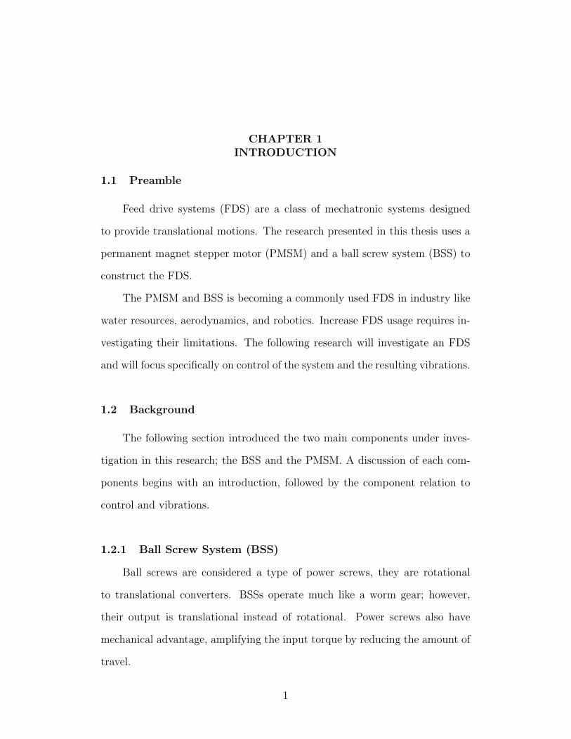
3.1.1 Adapted Ball Screw System Models
The block diagram in Figure 3–1 has a single input and a single output
for the BSS block. The BSS consist of four parts: the coupling, the ball screw,
the carriage, and the nut and screw interaction (NBSI) as shown in Figure
3–2. Each block has its own mathematical model.
Coupling Ball Screw NBSI CarriageInput Output
Figure 3–2: Block Diagram of BSS
Coupling
The coupling is the interface between the actuator and the ball screw.
An image of how the coupling connects the BSS to the PMSM is shown in
Figure 3–3. The coupling has mass, stiffness, and may have structural damping
[19]. However, the structural damping will be assumed to be zero for for this
research.
Figure 3–3: How a coupling connects the BSS to the PMSM.
13

The BSS model will combine the stiffness of the coupling, KC , with that
of the ball screw, KS. The stiffness of the ball screw and coupling will be
summed using theory for combining structural elements. Stiffness elements
can be added by taking the inverse of the individual summation of the inverse
stiffness values. The value of the new combined stiffness is given by:
KSC =
(1
KS
+1
KC
)−1
=KCKS
KC +KS
(3.1)
where KSC is the combined stiffness of the coupling and ball screw. Equation
3.1 could be used for both axial and torsional stiffness. KS depends on the lo-
cation of the carriage because the carriage is the only resistive force to counter
the motion of the ball screw causing twist. Calculating the stiffness becomes
more difficult requiring numerical analysis to obtain accurate results.
Quasi-static analysis is used to determine the stiffness elements of both
the ball screw and coupling. The ball screw can be modeled as a shaft and
hence the stiffness of shafts is given by:
KT =nGJ
L(3.2)
where KT is a generic torsional spring constant, n is the boundary condition
of the shaft ends, G is the modulus of rigidity, J is the moment of inertia of
the shaft, and L is the length of the shaft.
Ball Screw
14

The ball screw model was adapted by eliminating the carriage from the
model. The adaptation allows the ball screw model to be made of two com-
ponents: the ball bearings, and the ball screw, which can be seen in Figure
3–4.
Figure 3–4: FDB of ball screw
By neglecting the twist in the ball screw, the model now takes the follow-
ing form:
τinput = JSωS(t) + CBBωS(t) (3.3)
where τInput is the input torque applied from an external source, CBB is the
damping parameter of the ball screw, and KS is the stiffness of the ball screw.
A separate model is used to calculate the lateral modes. It is believed
that the lateral modes are the leading cause of vibrations in an FDS. Lateral
vibrations occur perpendicular to the BSS axis of rotation. Several modes can
be identified using the continuity equation for a simply supported beam:
15

f = nπ
√EI
mL(3.4)
where E is Youngs modulus, I is the moment of inertia of the beam, L is the
length, m is the mass per unit length, and n is the mode number.
Carriage
The ball screw is kinematically coupled to the motion of the carriage.
The kinematics of the carriage are coupled to the kinematics of the ball screw
through a constant γ:
γ =L
2π(3.5)
where L is the lead of the ball screw. The constant γ allows the rotational
motion of the ball screw to be mapped to the translational motion of the
carriage when there is no backlash.
The carriage model, which was developed from the free body diagram
(FBD) of the carriage as seen in Figure 3–5. The governing equation of motion
of the carriage could be obtained by applying a force balance as follows:
FC = MC x(t) + CLBx(t) (3.6)
where MC is the mass of the carriage, CLB is the damping coefficient of the
linear bearings, and FC is the force required to match the kinematics of the
16

carriage to the kinematics of the ball screw. The matching of kinematics,
between two systems, is referred to as kinematic coupling [20].
Kinematic coupling is not always valid because of the dynamics of other
components in the system. Specifically speaking about a BSS, axial forces can
lead to relative displacement between the translation of the carriage and the
rotation of the ball screw. The displacement comes from the axial force acting
in tension or compression on the ball screw.
Changes in acceleration are referred to as jerk. Jerk results in impact
forces being applied to the ball screw both in axial and torsional directions.
The reason the force acts in two directions is a result of the ball screw and
nut interaction. To reduce the effects of jerk in high speed operations, (the
focus of this research), the carriage needs to be designed from light-weight
components. The larger the carriage’s mass the greater the inertia, thus, the
greater the impact of jerk.
Figure 3–5: FDB of the carriage used to obtain the dynamic model.
Nut and Ball Screw Interaction (NBSI)
The NBSI is a complicated system to model. The system has ball bearing
traveling in groves along the helix of the ball screw. The exact helical groves
are mirrored inside the ball nut, as shown in Figure 3–6. The rotation of the
ball screw forces the ball bearing to contact the nut’s bearing groves. The
17

linear translational trajectory is maintained via the linear bearing guiding the
carriage.
The model adapted for the nut and ball screw interaction (NBSI) is a
static model. In order to ensure accuracy, careful consideration must be taken
into account when modeling a BSS to ensure accuracy. NBSI is very compli-
cated to model [21–24], for this reason a more conservative model has been
used [1, 3, 4]. NBSI has energy losses, thus, the governing equation is an effi-
ciency based formula:
ζ =FCL
τinput2π=FC
τγ(3.7)
where τinput is the input torque applied to the ball screw. The efficiency, ζ,
represents the ratio of input to energy transmitted from the input converted
into usable work. The loss of energy comes from the NBSI as a result of
contact between nut, ball bearing and screw as shown in Figure 3–6.
Figure 3–6: Example of interface between nut and screw through ball bearings[24].
The linear motion of the carriage results from restricting the carriage mo-
tion to one dimension. All other directions are limited by the linear bearing.
18

The linear bearings restrict the motion in all directions except axially.
3.1.2 Adapted Permanent Magnetic Stepper Motor Modeling
The block digram shown in Figure 3–1 illustrates a SISO system. How-
ever, PMSM are usually multiple input; single output (MISO). MISO systems
require more than one input to operate. A block diagram of a two phase
stepper motor as shown in Figure 3–7 has two inputs, one for each phase, but
has only one output a displacement, θ(t). Having multiple inputs causes the
PMSM to be more difficult to model and control than other electric motors.
Phase A
Phase B
Torque Convertor
Motor Mechanics
Input A Output
Input B
Figure 3–7: Block diagram of a PMSM.
Electric motors are composed of: rotor, stator, frame, and bearings. The
rotor rotates inside the frame of the motor and is supported by the bearing.
The stator is rigidly attached to the frame and remains motionless.
The actuation system used, for this research, is a PMSM. The PMSM
has many advantages and disadvantages associated with it (see Chapter 1).
The following section will discuss the basic operations of PMSM, followed by a
description of the model adopted from the literature. Figure 3–8 represents the
cross-section of a PMSM, where each tooth on the rotors has its own polarity.
Operation of a PMSM depends on the number of phases the PMSM con-
tains. The PMSM investigated in this research is a 2 phase motor with 200
steps per revolution. Each stator is an electromagnet with the ability to change
its polarity, and switch on or off. The rotor is a permanent magnet with teeth;
each tooth has the opposite polarity to adjacent tooth as shown in Figure 3–9.
19

Figure 3–8: General Schemcatic for 2 phase PMSM [1].
The PMSM motor requires individual phase inputs, which need to operate in
a specific sequence. The frequency of the pulses, and the number of pulses
governs the velocity and displacement, respectively.
Figure 3–9: Diagram of the teeth of the PMSM rotor and how they lock withthe stator.
Modeling a PMSM Electrical System
20

The circuit for the electromagnetic system is shown in Figure 3–10.
Coil Resistance
Ij(t)
Stator j
Supply
Figure 3–10: Circuit for single phase of PMSM.
The equation governing the interaction between the electrical elements of
the PMSM is given by:
V (t) = ε(θM) +RMI(t) + LM I(t) (3.8)
where V is potential difference across the phase, RM is the resistance phase,
LM is the inductance of the phase, and ε is the back electromotive force (EMF),
a function of the velocity of the PMSM rotor/shaft.
The back EMF, ε, created by the rotor, causing the stators to induce a
current from the changing magnetic field. The back EMF can be calculated
using:
ε = KM sin(φ+ nθ(t)
)θ(t) (3.9)
where KM is the motor constant, KM is the phase position, N is the number
of teeth on the rotor, and θ(t) is the rotors position. The motor constant will
be discussed in more detail in the next section.
Modeling of the PMSM’s Electro-Mechanical System
21

Shah [15] proposed a model for a stepper motor where the torque created
by the motor, τM could be determined using the following equations:
τM =n∑
j=0.5
(KMsin(φj +NθM(t)))Ij(t) (3.10)
where j refers to the specific phase, n is the total number of phases, and Ij(t)
is the current applied to the stator. The motor torque, τM , is the total torque
experienced by the PMSM shaft.
The motor constant was determined by assuming a linear relationship
between the torques and current of a phase [25]. For PMSM the holding
constant could be calculated by taking the quotient of the holding torque and
the current per phase. The motor constant, KM , allows the geometry and
electro-magnetic properties, between the stator and the rotor, to be simplified
into a single term:
KM =τHIR
(3.11)
where τH is the holding torque, and IR is the maximum rated current for the
PMSM.
Modeling of PMSM Mechanical System
The mathematical model for the mechanical system of the PMSM is de-
fined as:
τM = JM ωM(t) + CMωM(t) + τL (3.12)
where JM is the inertia of the rotor, CM is the damping coefficient, ωM is the
22

rotational velocity of the motor, τL is the external load attached to the motor
and τM is the applied torque from the motor. If there is no external load τL
can be removed from the equation.
3.2 Simulations Results
This section will discusses the final equation used for the simulations.
3.2.1 PMSM Simulation Results
Simulation of a PMSM motor requires the concatenation of equations 3.8
- 3.12. Unlike the BSS, simulation of the PMSM does not require rearranging
the models into sate space notation. The models discussed above focussed
on the physical construction of the PMSM. A PMSM, unlike a brushed DC
motor, requires more than one input in order to achieve motion. Figure 3–11
illustrates two methods for achieving motion of a PMSM. Position (b),(d), (f),
and (h), represent the PMSM full step operation on the PMSM. If position (a),
(c), (e), and (g) are injected into the sequence, yielding (a)(b)(c)(d)(e)(f)(g)
and (h), this method is referred to as half-stepping. The simulation results
were obtained using full stepping sequence.
A pulse function was developed to act as an experimental motor driver
for the PMSM, see Appendix A. The pulse function can be modified to give
the PMSM both halve. Unfortunately that is the limit of the pulse function.
Microstepping requires control over the current charging the circuit and thus
can not be controlled by the pulse generator.
The program to simulate the PMSM receives two inputs: time and di-
rection. Time is used to control the period of the phase and the direction
determined how phase B should respond. To keep the simulations simple the
signal for phase A and phase B are identical, they only have a phase difference
23

Figure 3–11: Demonstrates the required sequence for operation of a two phasePMSM.
shown in Figure 3–12. Figure 3–12 depicts how the pulse function is used to
simulate four steps of the PMSM. The first sequence is AB’, this phase exci-
tation corresponds to Figure 3–11(h). That means the rotor would now be in
the NW direction. The three remaining steps are AB, A’B, and A’B’. Each
of the remaining sequences corresponds the sequence in Figure 3–11 (b), (d),
and (f), receptively.
The pulse generator was designed to only deliver a unit value, see Ap-
pendix A. The reason Figure 3–12 amplitude is 24 Volts is because the poten-
tial able to be supplied and the data was collected after the voltage gain was
applied. Confirmation of the pulse generator functionality allows for several
assumption to be used in order to extract the final parameters required to
complete the PMSM simulation.
24

0 0.1 0.2 0.3 0.4 0.5−25
−20
−15
−10
−5
0
5
10
15
20
25
Time(s)
Vo
lta
ge
(V
)
Phase A
Phase B
Figure 3–12: Pulse frequency voltage delivered to the both phases.
Assumptions
There were several assumption utilized in the PMSM simulation. These
assumption are used in order to get preliminary results and ensure they are
comparable to the experimental data.
The assumption made are as follow:
1 A perfect chopping circuit can be implemented.
2 All electromagnetic properties in the system can be summed into a single
term, the motor constant and the response of the system related to the
rotational displacement is sinusoidal.
3 The damping experienced in the bearing, supporting the rotor behave
as a linear system.
25

4 The back EMF follows the model of equation 3.9.
Table 3–1: Parameters and values required for simulation of PMSM.
Coefficents Value UnitsJM 1.250 × 10⁻⁴ kg m2
L 1.639 × 10⁻⁶ HR 2.00 × 100 Ω
CMB 1.00 × 10⁻³ NmsKM 3.2 Nm/A
Methodolgy
The software used to conduct the simulation above was not used to con-
duct the following experiments, the first is to identify functionality of the
inputs. The code for this and all of the aforementioned code can be found
in Appendix A. In the beginning the proper sequence is delivered to the
phases, followed by an investigation of the phase coil responses to the input.
The torque will then be analyzed to identify the frequencies associated with
torque. Finally the displacement of the motor rotor will be observed.
Results and Discussion
The results for simulating the PMSM were obtained using the parameters in
Table 3–1.
Phase Response
Figure 3–13 shows the response obtained from an increasing pulse fre-
quency. As the pulse frequency increases the current no longer has the time to
reach its maximum value. After the frequency of the pulse crosses a frequency
of 98 Hz, the circuit no longer allows the coil circuit to charge to capacity.
The current of the coil is directly related to the output torque as defined in
26

equation 3.10. Therefore, if the current is not able to achieve the required
value to maintain synchronization, the motor will skip and stall.
Figure 3–13: Response of phase coil to increasing pulse frequency.
Increasing the input voltage allows the input pulse frequency to increase;
however, this results in the current exceeding the maximum current rating of
the motor.
In order to keep the current from exceeding the rated limit, a circuit called
a chopping circuit [26]. The chopping circuit restrict a circuit from exceeding
a given threshold. In addition it allows the fast response of a high potential
and still allows the PMSM to operate within specification. The result of the
same input signal to a PMSM with a chopping circuit can be seen in Figure
3–14.
The response of the phases may appear as a step response; however this
is not what is actually happening. Zooming in on the response yields that the
27

0 0.1 0.2 0.3 0.4 0.5−5
−4
−3
−2
−1
0
1
2
3
4
5
Time (s)
Cu
rre
nt
(A)
Figure 3–14: Response of phase coil to increasing pulse frequency with a chop-ping circuit.
system still response the same, the input has been amplified from 6 Volts to 24
Volts. By using the chopping circuit the coil model is not changed. However,
increasing the input decreases the amount of time required for the phase coil’s
current to reach the PMSM maximum allowable current.
With the available current for each phase, the developed torque is iden-
tified to that equation 3.10 can now be simulated. The developed torque is
going to be the torque that acts upon the PMSM rotor. Figure 3–15 shows
an example of the torque generated when a pulse frequency, starting at 0.8 Hz
and steadly increaing to 100 Hz, is applied to the PMSM.
The torque signal is a periodic signal that corresponds to the pulse fre-
quency. The spikes that occur every period are a result of the PMSM taking
28

0 5 10 15 20 25 30−1.5
−1
−0.5
0
0.5
1
1.5
2
2.5
Time (s)
To
rqu
e N
m
Figure 3–15: Sample data for the torque applied to the shaft of the PMSM
the next step. Closer inspection of the torque response reveals that all torques
respond in exactly the same way. The torque experienced by the rotor is zero,
then spikes before oscillating about zero before finally stopping at zero torque,
as shown in Figure 3–16. Another area of interest is the frequency of the os-
cillation about the zero torque position. This frequency is believed to be the
natural frequency of the PMSM, making this frequency disrupt the operations
of the PMSM.
Torque ripple is what occurs when a torque oscillates as a result of the
frequency being experienced by the rotor. The ripple refers to the vibrations,
which the PMSM exhibits in low speed operations. Figure 3–15 is the torque
data for an increase pulse frequency. As the frequency increase the torque
begins pulses become shorter and there is not enough time for developed torque
to reach zero before the next pulse appears. When to developed torque can
29

no longer oscillate before the next pulse initiates the torque ripple stop and
the vibrations they caused stop.
The minimum frequency required in order to avoid this phenomena was
shown to be 14 rad/s according to the data represented in Figure 3–15. It
should be noted that in order to simulate the PMSM the rotor dynamics need
to be applied, thus if an auxiliary load is applied overall natural frequency of
the new system will change.
0.8 1 1.2 1.4 1.6 1.8 2
−1.5
−1
−0.5
0
0.5
1
1.5
2
Time (s)
To
rqu
e N
m
Figure 3–16: Zoomed result of developed torque in order to identy the naturefrequency of the system.
Figure 3–15 demonstrates what happens to the torque signal when a pulse
signal with a frequency of 100 Hz is applied. If the pulse frequency increases
the torque no longer increases. The frequency which the torques are all pos-
itive is when the vibrations, caused by the reversing torque, are no longer
measurable. The frequency hereby known as the, operating frequency which
30

is defined as the frequency at which the motor can move at whatever length
of step without skipping. The back emf only begins to have a counter effect
after the PMSM no longer reaches a point of equilibrium, these results can
also be observed in the rotor response to the developed torque.
Rotor Displacement and Velocity
The rotor displacement was analyzed first for the response it had to work
at a frequency below the operating frequency. An investigation into the fre-
quency of the oscillation about the set point followed was conducted. This
was carried out in order to see if there was any correlation with frequency
developed from the developed torque.
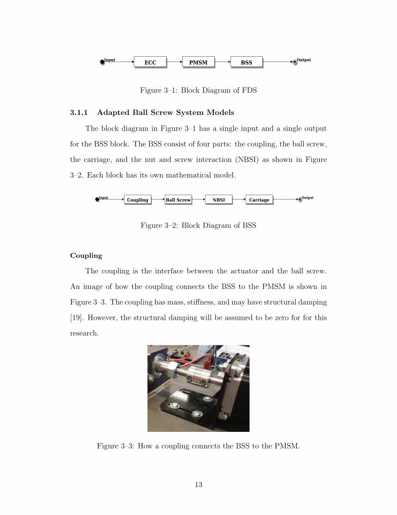
The rotor response, to pulse frequency below the operating frequency, can
be seen in Figure 3–17. As the pulse frequency increases from 1 Hz to 10 Hz
the response does not change, the only difference is the time which it takes for
the simulation to reach the final location.
Increasing the pulse frequency continues to reduce the transience of the
rotors rotation causing reduction of vibrations caused by torque ripple, as
shown in Figure 3–18.
The back-EMF has no practical effect on the PMSM until the velocity of
the system begins reaches above the to the therefore in order to get a more
accurate model of the actual rotational velocity of the the rotor a low pass
filter can be implemented to process the data collected for velocities under the
operating frequency as shown in Figure 3–19.
Maximum Pulse Frequency
31
0 0.5 1 1.5−5
0
5
Time (s)
Curr
ent (A
)
Phase A&B vs Time
0 0.5 1 1.50
1
2
3
4
Time (s)T
orq
ue N
/m
Torque vs. Time
0 0.5 1 1.50
10
20
30
40
Time (s)
θ (
radia
ns)
Angular Displacement vs. Time
0 0.5 1 1.50
20
40
60
80
Time (s)
ω (
rad/s
)
Angular Velocity vs. Time
Figure 3–17: Rotors displacement for varying frequency from 1 - 0.5.
32

0 2 4 6−4
−2
0
2
4
Time (s)
Curr
ent (A
)
Phase A&B vs Time
0 2 4 6−2
0
2
4
Time (s)T
orq
ue N
/m
Torque vs. Time
0 2 4 60
20
40
60
80
Time (s)
θ (
radia
ns)
Angular Displacement vs. Time
0 2 4 6−100
0
100
200
Time (s)
ω (
rad/s
)
Angular Velocity vs. Time
Figure 3–18: PMSM results for varying frequency from 0.1 - 0.01.
33
0 0.2 0.4 0.6 0.8−4
−2
0
2
4
Time (s)
Curr
ent (A
)
Phase A&B vs Time
0 0.2 0.4 0.6 0.8−4
−2
0
2
4
Time (s)T
orq
ue N
/m
Torque vs. Time
0 0.2 0.4 0.6 0.80
20
40
60
80
Time (s)
θ (
radia
ns)
Angular Displacement vs. Time
0 0.2 0.4 0.6 0.80
100
200
300
400
Time (s)
ω (
rad/s
)
Angular Velocity vs. Time
Figure 3–19: PMSM results for varying frequency from 0.01 - 0.001.
34
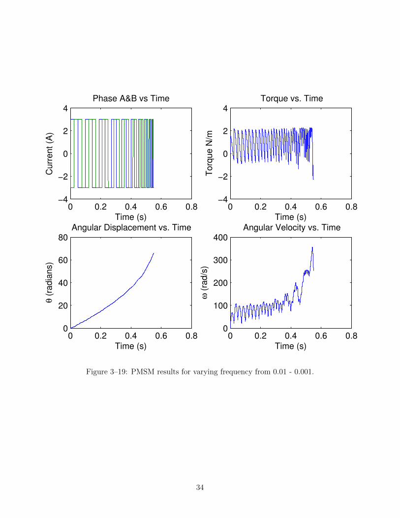
The maximum pulse frequency relates directly to the maximum velocity
the PMSM can achieve before losing synchronisation. When a PMSM ex-
periences a loss of the synchronizing the PMSM is said to have ”skipped”.
Depending on the velocity of the skipping, if the pulse frequency is too high
the rotor, of the PMSM, will not have enough time to reach the minimum
travel distance before the next step initates; This causes a constant oscillation
of the rotor with very minimal rotational displacement, see Figure 3–20.
The torque periodically varies from negative to positive, almost with a
zero mean value over a period. The rotor response to the torque leads to high
frequency vibration when the PMSM was allowed to reach steady state.
Damping Parameter Identification
All the parameter values used to simulate the PMSM can be justified with
some certainty except for the damping coefficient used for the ball bearing sup-
porting the rotor. Friction is a very difficult variable to model because it is
non linear, piecewise, and material dependent. Friction is almost always asso-
ciated with damping, and damping has little effect on the natural frequency
of a system, for this reason a range of damping coefficients were tested on the
simulation to demonstrate the effect of damping on the response of the PMSM
model as shown in Figure 3–21.
The damping parameter only effects the transient response and not the
frequency or the response time of the simulation itself. Only effecting the
transient decay time of the response allows the damping parameter to have
a large span of values without effecting the frequency response of the system
greatly.
35

0 0.02 0.04 0.06−4
−2
0
2
4
Time (s)
Curr
ent (A
)
Phase A&B vs Time
0 0.02 0.04 0.06−2
−1
0
1
2
Time (s)T
orq
ue N
/m
Torque vs. Time
0 0.02 0.04 0.060
0.1
0.2
0.3
0.4
Time (s)
θ (
radia
ns)
Angular Displacement vs. Time
0 0.02 0.04 0.06−20
0
20
40
60
Time (s)
ω (
rad/s
)
Angular Velocity vs. Time
Figure 3–20: PMSM results when failure occurs.
36

0.248 0.25 0.252 0.254 0.256 0.258 0.26 0.262
17.5
18
18.5
19
19.5
Time (s)
Dis
plac
emen
t (de
g)
Figure 3–21: Displacement simulation to observe the transience that happensfrom a single step.
37

3.3 Pre-processing Filter
The following section highlights the main contribution of this thesis, the
pre-processing filter (PPF). The PPF enables the PMSM, with any attached
load, to operate like a linear system, and enables the design of linear control
techniques to further improve the performance.
The PPF enables the velocity profile of the stepper motor to be deter-
mined based on the input signal. The input signal is then used to calculate the
pulse frequency required to operate the PMSM at a specific velocity mapped
to the pulse frequency (fP ). Figure 3–22 illustrates how the signal from the
feedback controller (FBC) is converted to a pulse frequency in order to input
the pulse frequency.
FBC
Encoder
PPFInput
SystemOutput
-
Figure 3–22: Block diagram used help visualize the functionality of the PPF.
The PPF was implemented by first using a block diagram to layout the
different constants and functions required for the PPF to operate. Figure 3–23
demonstrates how the program requires the use of several user inputs along
with a control signal. Those inputs are then routed to two functions: the
velocity mapping function and the ramping function.
Constants and Functions
The maximum velocity parameter and the control signal are used to cal-
culate the pulse frequency. The pulse frequency is modeled such that a linear
increase in the control signal corresponds to a linear increase in rotational
velocity. The equation used to calculate the is pulse frequency, fP , is:
38

Velocity Mapping Function
RampingFunction
s
Logic
¡ 500 0 50032767 0 32767
ωMAX
u(t)
Dead-Zone
fP
αRate
Figure 3–23: Process Flow Diagram for the PPF.
fP =KPPF (ωMAX)∣∣u(t)
∣∣ (3.13)
where KPPF is the gain used for specific PMSM’s and PPF configuration
and is determined experimentally, u(t) is the control signal, and ωMAX is the
maximum velocity also determined experimentally.
The ramping functions is more complicated than a simple mapping func-
tions. The ramping functions is calculated using the acceleration rate, αRate;
however, the actual value to ramp the pulse frequency at requires the change
in input signal, δu(t) which is mapped to the change in rotational velocity, δω
or α, of the PMSM. The equation used to calculate the pulse frequency step
size, δfsize, is:
δfsize =δu(t)
αRate
(3.14)
where αRate is the acceleration rate and δu(t) is the change in control signal.
The final parameter observed in Figure 3–23 is the PPF dead-zone. The
PPF dead-zone is a parameter that needs to be used in order to stop the
PMSM from operating a velocities too slow. When the PPF is receives a very
small control signal and is connected in a feedback configuration the system is
39

not able to stabilize and begins to oscillate about the setpoint at a frequency
equal to the that of the FBC. The reason for the instability is a result of
the feedback optical encoder. The resolution of the encoder is greater than
the precision of the PMSM thus each step results in a large overshoot of the
setpoint.
The PPF dead-zone is the applied to the velocity mapping function and
used to stop small signal from operating at these velocities. The final profile
for the mapping velocity function is shown in Figure 3–24. The deadzone
introduces a known linearity that eliminates the chatter about the setpoint;
however, the deadzone also decrease the precision of the PMSM.
−32767 0 32767− 67 0 3276767
Rot
atio
nal V
eloc
ity
ωMAX
Controller Signal
Dead-Zone
Figure 3–24: The velocity profile with both the dead-zone and velocity map-ping function concatenated.
There are many improvements and modifications that can be made to this
linear mapping program. The improvements will be discussed in the future
40

work section of Chapter 6. The remainder of the thesis will use the feedforward
controller(FFC) program to experimentally determine the constant values of
the PPF for two different systems and compare their results. Finally, linear
controllers will be implemented in series with the PPF and their performances
will be compared.
41

CHAPTER 4EXPERIMENTAL SETUP and METHODOLOGY
This chapter discusses the experimental setup and methodology used to
perform the experiments conducted in this thesis. The description of the ex-
perimental setup is presented first, followed by the methodology and procedure
used for the experiments.
4.1 Experimental Setup
There are three subsystems used to construct the experimental setup,
hereby referred to as the apparatus. The three subsystems are mechanical,
electrical, and control. Each of the three subsystems will be described, fol-
lowed by a section on data acquisition. Figure 4–1 illustrates the number of
components used to construct the FDS.
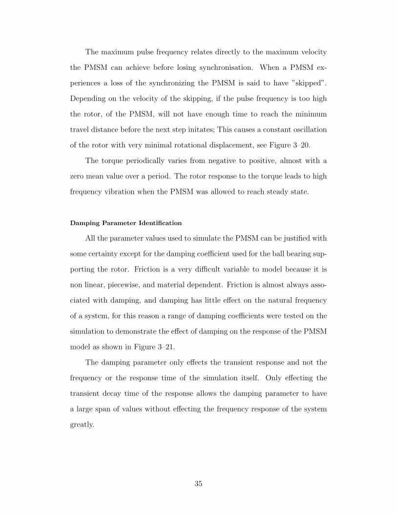
4.1.1 Mechanical
The mechanical subsystem is composed of the frame, the BSS, and the
PMSM as shown Figure 4–2. This subsection will discuss the design criteria
for each component followed by an explanation for the final design selection.
42

Figure 4–1: The experimental setup showing the particular components.
The Frame
The frame was designed to meet the following criteria:
• Level
In order to avoid the affects of gravity the system was to be completely
level. If the carriage is not completely level, and the setup is motionless
their would always be a constant force acting on the ball screw and
propagating throughout the rest of the system.
• Rigid
Testing for the sources of vibrations requires that all moving compo-
nents be mounted rigidly to the frame. If the components are not rigidly
mounted to the frame there will allow and unwanted vibrations.
• Adjustable
Not all workstations are level and may even be composed of multiple sur-
faces. Having the frame pegs adjustable ensures level operations. Steel
43
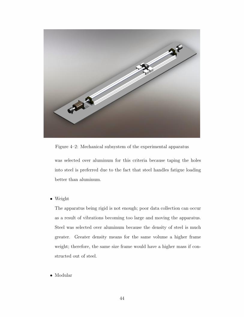
Figure 4–2: Mechanical subsystem of the experimental apparatus
was selected over aluminum for this criteria because taping the holes
into steel is preferred due to the fact that steel handles fatigue loading
better than aluminum.
• Weight
The apparatus being rigid is not enough; poor data collection can occur
as a result of vibrations becoming too large and moving the apparatus.
Steel was selected over aluminum because the density of steel is much
greater. Greater density means for the same volume a higher frame
weight; therefore, the same size frame would have a higher mass if con-
structed out of steel.
• Modular
44

When designing a system there are situation requiring the alteration of
the design. In order to alter the design the work piece must be easier
to work with. Steel was selected over aluminum because steel is less
subseptable to failure from repetitive use.
The frame final design was constructed out of steel because it fulfilled
more of the design criteria.
The Ball Screw System (BSS)
Design of the BSS is heavily dependent on the application of the BSS.
The main objective of this research was to investigate motion control and
vibrations. Motion control requires a large span of travel to investigate the
ramping abilities of a PMSM. Vibrations investigation requires that the ball
screw not be to large in diameter. If the diameter is too large, the system may
not be able to reach the velocities required to excite resonance and unbalanced
rotating vibrations.
The ball screw selected was an MSC ball screw; specifications can be seen
in Table 4–1. The nut was selected based on the selected ball screw because
the ball bearing inside the nut, must match-up with the grooves of the ball
screw. The exact specification of the ball screw can be seen in Table 4–2.
Table 4–1: Specification of the ball screw used in the experimental setup.
Ball Screw Parameter Value UnitsLead Width 20 mm
Length 1220 mmDiameter 20 mm
Ball Bearing Diameter 1.60 mm
45

Table 4–2: Specification of the nut screw used in the experimental setup.
Ball Nut Parameter Value UnitsNut Length 60 mmNut Width 40 mm
Flange Length 30 mmBall Bearing Diameter 1.60 mm
The carriage was not designed until the apparatus was completely assem-
bled. The carriage had a several design constraints influencing:
• Size
The first constraint was size. The length of the ball screw only allowed
for a 1000 mm of travel, minus the linear bearings and ball nut. In order
to maximize travel, the carriage had to be no greater then the size of
the linear bearing and ball nut, see Appendix B.
• Weight
By having the carriage lightweight a larger acceleration can be imple-
mented without slipping. Larger accelerations mean superior perfor-
mance when traveling smaller distances.
• Robust
The final constraint was being simple. The design was kept simple be-
cause of the precision the part required. Connecting four independent
components together requires extreme precision and accuracy.
The criteria mentioned above have led to the conclusion that wood was
used as the material for the carriage. Wood was forgiving, easy to work with,
46
cheap, and available.
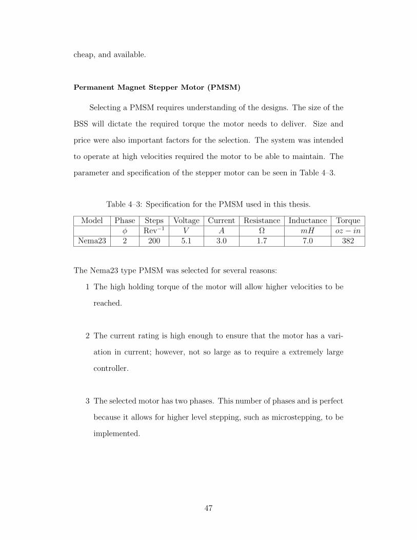
Permanent Magnet Stepper Motor (PMSM)
Selecting a PMSM requires understanding of the designs. The size of the
BSS will dictate the required torque the motor needs to deliver. Size and
price were also important factors for the selection. The system was intended
to operate at high velocities required the motor to be able to maintain. The
parameter and specification of the stepper motor can be seen in Table 4–3.
Table 4–3: Specification for the PMSM used in this thesis.
Model Phase Steps Voltage Current Resistance Inductance Torqueφ Rev−1 V A Ω mH oz − in
Nema23 2 200 5.1 3.0 1.7 7.0 382
The Nema23 type PMSM was selected for several reasons:
1 The high holding torque of the motor will allow higher velocities to be
reached.
2 The current rating is high enough to ensure that the motor has a vari-
ation in current; however, not so large as to require a extremely large
controller.
3 The selected motor has two phases. This number of phases and is perfect
because it allows for higher level stepping, such as microstepping, to be
implemented.
47
4 The final reason is because of the step size. Having a motor capable of
200 steps per revolution gives great accuracy especially if the mechani-
cal advantage of the ball screw is considered. Also from the research the
most predominant number of steps for stepper motors is 200.
4.1.2 Electrical
The Electrical assembly is made of three things:
Power Supplies
The power supply is a BK Precision 1672 supplying 3 amp of current for
and up to 90 watts of power. If more current is required the system can be
bridged for a total of 6 amps. The power supply is only used to power the SMD.
Stepper Driver
The stepper driver is a BL-TB6560 , SMD. The SMD was selected because
of its versatility. Ability to operate at multiple current levels is an excellent
advantage when it comes to validating models. Controlling the current allows
the testing of the parameters such as hold torque, to be tested varying multiple
parameters.
Ability to perform microstepping makes it possible to conduct future re-
search to further optimize the controller designs. The TB-6560 has the ability
to operate with four different stepping profiles: full, half, 18, and 1
16. This also
save the task of having to program the stepper motor sequence, freeing an
additional microcontroller.
The TB-6560 is simple to operate, only requiring the use of 3 digital pins
used to: activate or deactivate pin, clockwise or counter-clockwise pin, and a
step pin. The step pin receives a HIGH input, and takes a step, then until a
48

change occurs and the pin goes HIGH another step will not be taken.
4.1.3 Control
The controller is composed of three subsystems: the feedback controller,
the preprossesing filter, and the motor driver.
PPF Controller
Pre-processing filters was implemented on the on a ATmega328. The
ATmega328 uses an 8 Mhz single core processor is used calculate the mapping
velocity function, calculate the ramping function, store state data, and receive
signal through I2C protocols.
FBC
The FBC is the slowest of the three operating frequencies. This controller
can be designed using any method of controller requiring error as feedback.
For this research it was programmed with a slow refresh rate; the refresh rate
will be discussed more later in more detail. The controller used for this re-
search are:
• Proportional Controller (P)
• Proportional Derivate Controller (PD)
Two microcontrollers are controlling the system. More specifically a AT-
MEL328P is being used as the pre processing filter (PPF). The second con-
troller was an ATMEGA 2560 and was used as the feedback controller.
49

4.1.4 Data Acquisition
All of the data was collected using NI USB-6341. The NI USB-6431
is equipped with a 12 bit A/D. The DAQ is not used for control purposes
because of the delay caused by the serial information need to pass to the PC.
Although capable of controlling the system, predicting the resources allocation
is difficult. This is because of all the buffering required in order to operate
over serial communication as a protocol the system must do in order to relay
that information to the computer.
All of the data was collected using LabView, and was analyzed using Mat-
lab. The VI for the data collection program is located in Appendix A. The
only variable parameter was the collection frequency. The collection frequency
was created to ensure that the buffering of the NI USB-6341 does not become
congested with to much data.
Accelerometer
Accelerometer are Dytran PIEZO 3225F1 transducers. Two accelerome-
ters were used throughout this research. The first is a uni-axial accelerometer.
The second was a tri-axial accelerometer. There is very little difference be-
tween the two accelerometers; however, the tri-axial accelerometer can save
time by collecting three signals at once. The specification for the accelerome-
ters can be found in Table 4–4.
Table 4–4: Specification of the accelerometers used in the following disserta-tion.
Accererometer Value UnitsSensitivity 9.77 mV/gDiameter 1.00 × 101 mm
Max Frequency 10000 MHz
50

Optical Encoder
There were two optical encoders used: one to collect the data from the
PMSM, and the other to collect the displacement information of the ball screw.
The encoders are both identical quadrature encoders with resolutions of 600
ticks per revolution; however, when both encoder phases are used, the resolu-
tion increase to 2400 ticks per revolution, resulting in a resolution +/- 0.00262
radians
Table 4–5: Specification for Optical Encoder
Optical Encoder Value UnitsType Quadrature
Resolution 600 Pulses/RevDiameter 4.0 cm
All of the data collected was done through the use of a National Instru-
ments USB-6341. Theses data include: (a) the displacement data for the from
the optical encoder coupled to the PMSM, (b) the vibrations information was
also collected using the NI USB-6431.
4.2 Methodology and Experimental Procedures
The following section presents the experiments conducted in this the-
sis. The experiments have been placed into several categories: Experimetnal
Validation, Feedforward Parameter Extraction, Controller Design, and Vibra-
tions Analysis. Each category will begin with an introduction, followed by the
methodology and experiments related to that category.
Figure 4–3 contains a flow chart containing all of the different experi-
ments; however, because the experiments for both the FDS and the PMSM
are identical the flow chart can implemented on either system. All of the anal-
ysis and experiments are based of the validation of the experimental setup.
51

4.2.1 Experimental Validation of the Apparatus
Experimental validation was used to ensure that the data collected for all
of the experiments was accurate. Without validation there was no way to be
certain that the developed experiments are functioning properly, or that the
analyzed data is correct. The experimental validation section contains three
experiments: data acquisition validation, displacement validation, and veloc-
ity validations.
Data Acquisition Validation
Data acquisition validation was required to ensure that the NI-USB-6341
was recording the correct information. The experiments for the validation
involved recording the displacement of the PMSM for different collection fre-
quencies. The PMSM was stepped at every 0.5 seconds, the first experiments
were conducted for collection frequencies of 1 kHz, 333.3 Hz, and 166.7 Hz.
The final results were compared simultaneously in the same figure.
The second experiment was to compare the recorded response to the sim-
ulation result obtained in Chapter 3. The simulation were conducted using a
step size of 0.125 seconds, as was the experimental data and the two sets of
data were superimposed on the same figure and the results were discussed.
Displacement and FFC Validation
Displacement validation ensures that the all the collected data from the
optical encoder is functioning correctly. The FFC was used to validate the
displacement of the PMSM. A PMSM has 200 steps per revolution and one
revolution equates to 6.283 radians.
The displacement experiments were conducted by using the FFC to move
200 steps with a velocity of 1 rad/s to ensure no slipping occurred. The
52

experiment was then compared to the recorded value from the optical encoder.
At low velocities the PMSM 200 steps should equate to 6.283.
The FFC validation was conducted to determine the velocity threshold
for FFC operations. The experiment were conduct by ranging the velocity
from 1 rad/s to 60 rad/s and the result were reanalyzed to see if the FFC con-
tinued to function reliably in feed forward mode. When the recorded values
no longer match the value set by the FFC, the system can no longer operate
in FF mode. The result were concatenated onto a single figure to illustrate
the FFC operation thresholds.
Velocity Validation
Velocity validation is used to determine the whether the prescribed veloc-
ity setting of the FFC equals that of the optical encoder. The optical encoder
data contained displacement information. Extracting the velocity from the
displacement signal requires numerical differentiation. When the displace-
ment signal was differentiated there was significant amount of noise imposed
over the velocity signal. To eliminate the a noise fourth order Butterworth
filter was applied to the velocity signal and tuned until the velocity setpoint
could be identified. The velocity setpoints were then compared to the FFC’s
velocity. Several velocity setpoints were chosen ranging from 0 to 40 rad/s.
The relationship was identified through curve fitting and a correlation was
established so that the actual velocity could still be identified based on the
FFC’s input velocity.
53
4.2.2 Feedforward Parameter Identification
Feedforward Parameter Identification is a technique used to identify dif-
ferent characteristics of the PMSM and the FDS. The remainder of the ex-
periments in this thesis are all conducted using the PMSM and the FDS and
will hearby referred to as the systems. The FFC program was enhanced for
simplistic manipulation of: the maximum velocity and the acceleration, see
Appendix A. Tuning of these parameters allows the PMSM to be optimized
for specific applications.
Maximum Velocity
The maximum velocity is the largest rotational velocity the shaft of the
PMSM can achieve before slipping. Each PMSM will have a different maxi-
mum velocity because of the physical characteristics of the PMSM. PMSMs
are used to control and operate external loads attached to its shaft; the load
attached to the PMSM will also affect the maximum velocity [15].
Identifying the maximum velocity of the PMSM is important because
it is used to help design the PPF. The maximum velocity was also a great
measurement, which can be used when comparison of the systems performance.
There were several experiments conducted to identify the maximum velocity.
The first experiment involved localizing the maximum velocity by increasing
the velocity slowly at, acceleration rate of 2000, until the rotor of the PMSM
stalled and skipped. In order to better identify the velocities, Butterworth
filters were applied to the velocity signals of the systems.
The next experiments involved refining the newly hypothesized maximum
velocity for each system. This was achieved through decreasing the hypothe-
sized maximum velocity by 5% and tuning. When the velocity was obtained
from the previous experiments the final experiment was to confirm if a larger
54

velocity could be achieved by further increasing the acceleration rate.
Maximum Acceleration
The maximum acceleration governs the maximum rate that the velocity
can change. The maximum acceleration depends on the physical character-
istics of the PMSM and will change from a PMSM to a PMSM. Much like
the maximum velocity, the maximum acceleration will be affected by different
loads connected to the PMSM.
There was only one set of experiments conducted for identification of
the maximum velocity. The acceleration of the systems are determined by
identifying the maximum velocity jump the PMSM can achieve in a single
step. For this reason the units for the maximum acceleration are given as
rad/s/step.
Starting with an initial velocity of 0 rad/s the FFC was used in instan-
taneously jump from 0 to the maximum possible velocity. This maximum
velocity was identified through several trail and error experiments. Following
this the initial velocity was increased and the test was conducted again using
a new initial velocity. The initial velocity was ranged from 0 to 30 rad/s.
Following the experiments the results were tabulated. The difference between
the initial velocity and the maximum velocity was plotted against the initial
velocity and the results were analyzed.
4.2.3 Controller Design
The controller parameters were tuned manually. After which the per-
formance of the FSD and PMSM are compared using several criteria; fastest
response, minimum overshoot, settling time, and stability.
55

The controller implemented was used for precise positioning. The FDS
does not have unlimited travel making it difficult to conduct the experiments
using a velocity setpoint. There are four parameters used in the feedback con-
troller. Three of the parameter are gains; proportional, integral, and deriva-
tive. The final parameter is the feedback frequency. This frequency allows the
controller to decide how frequently to update the PPF. For this reason exper-
iments were conducted to determine the performance of the controller, and
PPF. However another dimension had been added to the analysis by allowing
a controller frequency to be variable.
PPF Parameter Identification
The PPF parameters need to be tuned just like the FFC parameters. The
PFF details were discussed previously in this chapter; however, identification
of the parameters has to be obtained experimentally.
The PPF is the linearization hardware allowing simple feedback con-
trollers to be implemented. The PPF is the heart of the control system, it
affects the performance of the entire system. The main parameters of interest
are identifying the minimum control value to achieve motion. Identification of
this parameter is required to help design the feedback controllers integral gain
and windup parameter. The controller will only function for values greater
then deadzone. If the control signal is not greater than the deadzone thresh-
old the system will not function. The tuning of the PPF requires the use
of another program, the manual input prepossessing filter (MIPPF), see Ap-
pendix A. This program allows the input value of the PPF to be manually
controlled. By having control of the controller signal the parameters for the
PPF can now be tested and tuned more efficiently.
56

The first set of experiments involved identification of the maximum veloc-
ity. The maximum velocity obtained from the FFPI experiment was used as
the initial velocity used to begin tuning the PPF. The testing was conducted
using the MIPPF’s maximum control signal. If the system reached maximum
velocity without stalling the PPF’s maximum velocity was increased; if the
system could not reach the PPF’s maximum velocity the setpoint was then
decreased until the PPF’s maximum velocity was obtained.
The acceleration rate was determined by first identifying the maximum
velocity. The systems were then set to an acceleration. To test for failure,
the MIPPF was used to operate the systems at their maximum input signal.
After the systems reached steady state, the MIPPF was then set from 30000
to -30000. By switching instantaneously from positive to negative, the accel-
eration can be fully tested. The responses were observed for failure. The trails
continued until the optimum acceleration rate was obtained.
After identifying the parameters for each system, the displacement data
was collected and the rotational velocity and acceleration were both extracted
and compared to the result from the feedfoward parameter identification ex-
periments.
Proportional Controller
A proportional controller was developed in order to test basic controller
performance. The proportional controller gain, KP , was ranged from 0 to 10
and the displacement was recorded.
After the experiments were conducted the analysis of the data consist-
ing of identifying the following parameters: time to peak tp, settling time, %
overshoot, and stability. The settling time and the time to peak were both
extracted from the raw displacement data collected. The setpoint was more
57

difficult to obtain because of the saturation limits of the systems. The max-
imum velocity and accelerations were reached by the systems quickly. When
this occurred the displacement acquired needs to be subtracted from the set-
point.
The setpoint in the data is not the actual setpoint used to calculate the
% overshoot of the experiment. The system behaves linearly; however based
on the configuration of the electrical system the system can only operate at
velocities under 60 rad/s. Reaching 60 rad/s using the current configuration
occurs very quickly. When the controller is saturated and the PMSM was
cruising at maximum velocity, the displacement made during this saturation
time is ignored giving a much more accurate representation of the % overshoot.
The final data collected from the proportional experiments was utilized
to assess the system stability. The system was considered unstable when the
PMSM would stall and skip.
Proportional Derivative Controller
The proportional derivative (PD) controller is a robust controller used to
allow greater performance by allowing the proportional gain to be set higher.
The derivative gain decrease the overshoot and oscillation caused by the high
proportional gain. The derivative gain uses the change in error to calculate
the addition to the controller output.
The experiment conducted using the PD controller allow for even greater
performance than the P controller could achieve alone. Observing the result
will help to determine if there is any benefit to adding the derivative gain.
58

Expe
rim
e ...
Dis
pVal
Velo
Val
FFCV
al
FFPI
Max
Vel
Max
Acc
VibI
nfo
PPFT
unin
gM
axVe
lPPF
Max
AccP
PF
Feed
back
...
Com
pari
son
P PD
Fig
ure
4–3:
Flo
wch
art
dem
onst
rati
ng
the
relian
ceof
each
exp
erim
ent
for
this
thes
is.
59

CHAPTER 5RESULTS and DISCUSSION
This chapter presents the results for the experiments conducted in this
thesis. The experiments are presented in the same order as described in Chap-
ter 4. Each experimental results will be followed by a detailed discussion. For
more detailed information into the methodology and procedures of the exper-
iments refer to Chapter 4.
5.1 Apparatus Validation
5.1.1 Data Acquisition Validation
The results of varying the sampling frequency of the data acquisition soft-
ware is shown in Figure 5–1. It was determined that when the data acquisition
software’s sampling frequency was set too high, a timing error begins to prop-
agate and leads to inaccurate results. Tuning the sampling frequency yielded
that a sampling frequency of 333 Hz stopped the timing issues and still main-
tained enough information to observe the forced input frequency.
5.1.2 Displacement Validation
The results of using the FFC to displace the PMSM’s rotor at an oper-
ating velocity of 1 rad/s are shown in Figure 5–3. For an FFC input of 200
steps, the optical encoder recorded a value of 1 revolution or 6.283 radians.
When the velocity was increased the same displacement of 6.283 radians con-
tinued to be observed until a velocity of 22.8 rad/s was reached. At a velocity
of 22.8 rad/s, the recorded value no longer matched that of the FFC. Figure
60

2.46 2.48 2.5 2.52 2.54 2.56 2.58
0.16
0.17
0.18
0.19
0.2
0.21
Time (second)
Dis
plac
emen
t (R
ad)
1 mS3 mS6 mS
Figure 5–1: Angular displacement profile for different sampling frequencies.
5–4 illustrates the PMSM’s feedforward reliability against rotational velocity.
As the operating velocity of the PMSM was increased beyond 22.8 rad/s, the
recorded response no longer consistently equaled 6.283 radian. As the velocity
was increased past 28.6 rad/s, the PMSM recorded displacement had a con-
stant error associated with it. The error between the input displacement and
the recorded displacement was always negative, implying that the PMSM’s
rotor overshot the displacement setpoint. Overshooting the setpoint is a re-
sult of the rotor’s inertia; the holding torque developed in the PMSM was not
enough to instantly stop the PMSM’s rotor in the desired location and caused
the PMSM to slip.
61

0 0.5 1 1.50
0.05
0.1
0.15
0.2
0.25
0.3
0.35
0.4
Time (s)
Dis
pla
ce
me
nt
(ra
ds)
Experimental
Simulation
Figure 5–2: Rotational displacement results versus simulations for samplingfrequency of 333 Hz.
5.1.3 Velocity Validation
The results of a velocity signal are shown in Figure 5–5. When the dis-
placement signal was differentated high frequency oscillations were observed
between 0.35-0.6 second. In order to identify the actual maximum velocity,
a fourth order butterworth filter was applied to the differentiated signal as
shown in Figure 5–6. An observation was made when applying the Butter-
worth filter to the signal: as the cut-off frequency of the butterworth filter was
decreased, the PMSM’s rotor dynamics became apparent.
Table 5–1 presents the data from multiple velocity setpoints and com-
pares them to the acquired velocity signal after a filter was applied. When the
difference was plotted against rotational velocity as in Figure 5–7, a non-linear
62

0 1 2 3 4 5 60
1
2
3
4
5
6
7
X: 3.292Y: 6.283
Time (s)
Dis
pla
ce
me
nt
(ra
d)
Figure 5–3: FFC displacement response at a velocity of 1 rad/s.
growth in error was observed as the velocity increased. When a polynomial fit
was applied to the sequence, an R2 value of 0.999. The equation of the line is:
ωActual(ωFFC) = (−103ω3FFC + 0.001ω2
FFC − 0.006ωFFC) − ωFFC (5.1)
Table 5–1: Result of velocity error for different target velocities.
FFC Setpoint (rad/sec) Experimental Value (rad/sec) Difference (rad/sec)0 0 02 1.99 10−4
5 4.99 10−3
10 9.97 0.0320 19.8 0.2530 29.5 0.5340 39.2 0.83
63

Rotational Velocity, (rad/s)
Feed
forw
ard
Co
ntr
oller
Ou
tco
me
Perfect
Unreliable
Fails
15 30 45
Figure 5–4: Illustration of the operating capabilities of the PMSM with respectto operating velocity.
At low velocities the difference between the FFC setpoint and the experi-
mental values was negligible. The negligible difference proves that the optical
encoder produced accurate results. The reason for the difference at high ve-
locities is a result of the computational time it takes the FFC to calculate the
velocity. The delay used to act as the velocity setpoint decreases as the ve-
locity increases; therefore, even though the velocity calculation take the same
amount of time, regardless of the velocity setpoint, the decrease in the delay
makes the calculation time affect the actual operating velocity.
5.2 Feedforward Parameter Identification
This section uses the feedforward controller to identify the maximum
velocity and the maximum acceleration the systems (PMSM and FDS) can
achieve. The details for the experimental methodology and procedures can be
found in Chapter 4 under the same section heading.
64

0 0.2 0.4 0.6 0.8 1 1.2 1.4 1.6−5
0
5
10
15
20
25
30
35
Time (second)
Velo
city (
rad
/s)
Figure 5–5: Differentiated displacement signal before being filtered.
5.2.1 The Maximum Velocity
PMSM
The results of the first maximum velocity experiment, using an acceler-
ation rate of 2000 and the velocity ramped from 30 rad/s to 100 rad/s, are
shown in Figure 5–8. From the plot it appears as though failure occurs at 55
rad/s. Note the large noise band of the signal. By applying the filter the noise
is removed.
The next experiments were conducted to further isolate the actual max-
imum velocity. By starting at 5 % below the estimated maximum velocity,
which was determined to be 56.7 rad/s. In order to determine the actual
velocity, a Butterworth filter was applied to these experiments as well. A
comparison of a filtered and unfiltered signal is shown in Figure 5–9.
65

0 0.2 0.4 0.6 0.8 1 1.2 1.4 1.6−5
0
5
10
15
20
25
30
35
X: 0.451Y: 29.47
Time (second)
Ve
lco
ity (
rad
/se
c)
Figure 5–6: Response of velocity profile for PMSM after applying a Butter-worth filter.
The velocity of 56.7 rad/s is the highest velocity the PMSM can achieve
before the affects of the back EMF and the damping cause the PMSM to
slip. Therefore, this is not an ideal operating velocity because any external
disturbance can lead to failure of the machine. For this reason, a more practical
value for the maximum velocity is needed. Choosing the maximum velocity
for feedforward operations was selected by taking 5% off the highest obtained
maximum velocity of 56.7 rad/s. The final velocity selected for the FFC was
in the velocity of 53.9 rad/s.
FDS
The maximum identifiable velocity is 62.85 rad/s. At this velocity the cur-
rent and power supply have been stretched to their limits and can no longer
handle inertial fluctuation or external disturbances. In order to achieve the
66

0 5 10 15 20 25 30 35 400
0.1
0.2
0.3
0.4
0.5
0.6
0.7
0.8
0.9
Velcoity (rad/s
Diffe
ren
ce
(ra
d/s
)
Figure 5–7: Difference between actual velocity versus FFC velocity.
velocity of 62.85 rad/s, the acceleration of PMSM had to be decreased. Unlike
the experiments conducted with the PMSM, the results of adding a load to
the PMSM’s shaft have been shown to greatly affect the acceleration of the
FDS. The practically selected maximum velocity for the FDS was 5% of the
absolute maximum velocity.
5.2.2 Maximum Acceleration
PMSM
The results for determining the maximum velocity the PMSM can achieve
from an intial starting velocity are shown in Table 5–2.
As the initial velocity of the PMSM is increased from 0 to 8 rad/s, it was
assumed that the maximum achievable velocity would also increase; however,
67
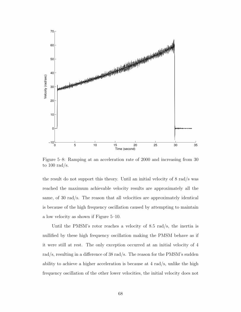
0 5 10 15 20 25 30 35−10
0
10
20
30
40
50
60
70
Time (second)
Velc
oity (
rad/s
ec)
Figure 5–8: Ramping at an acceleration rate of 2000 and increasing from 30to 100 rad/s.
the result do not support this theory. Until an initial velocity of 8 rad/s was
reached the maximum achievable velocity results are approximately all the
same, of 30 rad/s. The reason that all velocities are approximately identical
is because of the high frequency oscillation caused by attempting to maintain
a low velocity as shown if Figure 5–10.
Until the PMSM’s rotor reaches a velocity of 8.5 rad/s, the inertia is
nullified by these high frequency oscillation making the PMSM behave as if
it were still at rest. The only exception occurred at an initial velocity of 4
rad/s, resulting in a difference of 38 rad/s. The reason for the PMSM’s sudden
ability to achieve a higher acceleration is because at 4 rad/s, unlike the high
frequency oscillation of the other lower velocities, the initial velocity does not
68

0 5 10 15 20 25 30 350
10
20
30
40
50
60
70
Time (second)
Ve
lco
ity (
rad
/se
c)
Unfiltered
Filtered
Figure 5–9: Example of filtered signal superimposed on a non-filtered signal.
nullified the inertia but enhances it. The enhancement is due to the rotor’s
positive acceleration adding to the torque being implied to the rotor from the
new setpoint as shown in Figure 5–11.
Figure 5–12 represents the velocity difference acceleration versus the ini-
tial velocity. For the purposes of this project the initial velocity of 4 rad/s will
be ignored, and the remainder of the data will be interpreted. The parabolic
trajectory of the plot reveals a maximum at value of 16 rad/sec, and a min-
imum at an initial velocity of 27.5 rad/s. The acceleration rate ranged from
27.5 - 38 rad/s/step. For the practicality of this project, an acceleration of
27.5 rad/s/step was chosen because when in operation, the PMSM will poten-
tially sweep through all possible velocities thus leading to slipping and stalling.
69

Table 5–2: Results for dynamic velocity of PMSM
Initial Velocity rad/sec Maximum Velocity rad/sec Difference rad/sec0 30 304 42 386 32.5 26.58 32 24
8.5 33 24.59 35 2610 38 2812 42.6 30.616 48.2 32.220 50.0 3024 51.5 27.5
FDS
The results for the maximum acceleration of the FDS are shown in Table
5–3. The addition of an inertial load caused a different acceleration trend
as shown in Figure 5–13. The selection of acceleration was chosen to be 25
rad/s/step based on the minimum observed through experimentation.
Table 5–3: Results for dynamic velocity of PMSM
Initial Velocity rad/sec Maximum Velocity rad/sec Difference rad/sec0 40.5 40.54 41.5 37.58 42.5 34.512 44.5 32.516 45.5 29.520 48.4 28.424 51.0 27.028 53.1 25.132 55.0 23.0
5.3 Feedback Controller Results
This category of experiments presents the result from the chapter 4. The
section is divided into the 3 different experiments. Each experiment sections
70

0 0.5 1 1.5 2 2.5 30
0.05
0.1
0.15
0.2
0.25
Time (second)
Dis
pla
ce
me
nt
(Ra
d)
Figure 5–10: Results of stepping PMSM to demonstrate the effects of operatingat a low velocity.
is further divided into the results for the PMSM and the FDS.
5.3.1 PPF Tuning
PMSM
The results of tuning the PPF did not correlate with the FFPE values ob-
tained from the previous experiments. Both values were lower than the FFPE
values as a result of the PPF. Using a three stage controller caused timing
issues. These timing issues led to the discrepancy between the feedforward
parameters and the feedback parameters.
FDS
71

5.51 5.52 5.53 5.54 5.55 5.56
0
10
20
30
40
50
Time (second)
Ro
tatio
na
l V
elo
city (
rad
/s)
Figure 5–11: Data collected for acceleration experiments with an initial veloc-ity of the 4 rad/s.
Table 5–4: PPF parameters used for PMSM FBC.
PPF Value Measured VelocityAcceleration Rate 25 400 rad/s2
Maximum Velocity 80 58 rad/s
The result, for tuning of the FDS’s PPF parameters, are shown in Table
5–5. Although the parameter values changed, from the FFPI experiments, the
relationship between the PMSM and FDS parameter remained the same: the
maximum velocity increases and the acceleration decreases. Again the results
dropped from the results of the FFPI; however, the parameters maintain the
same relationship when compared to the PMSM parameters. The maximum
velocity is greater and the maximum acceleration is less.
72
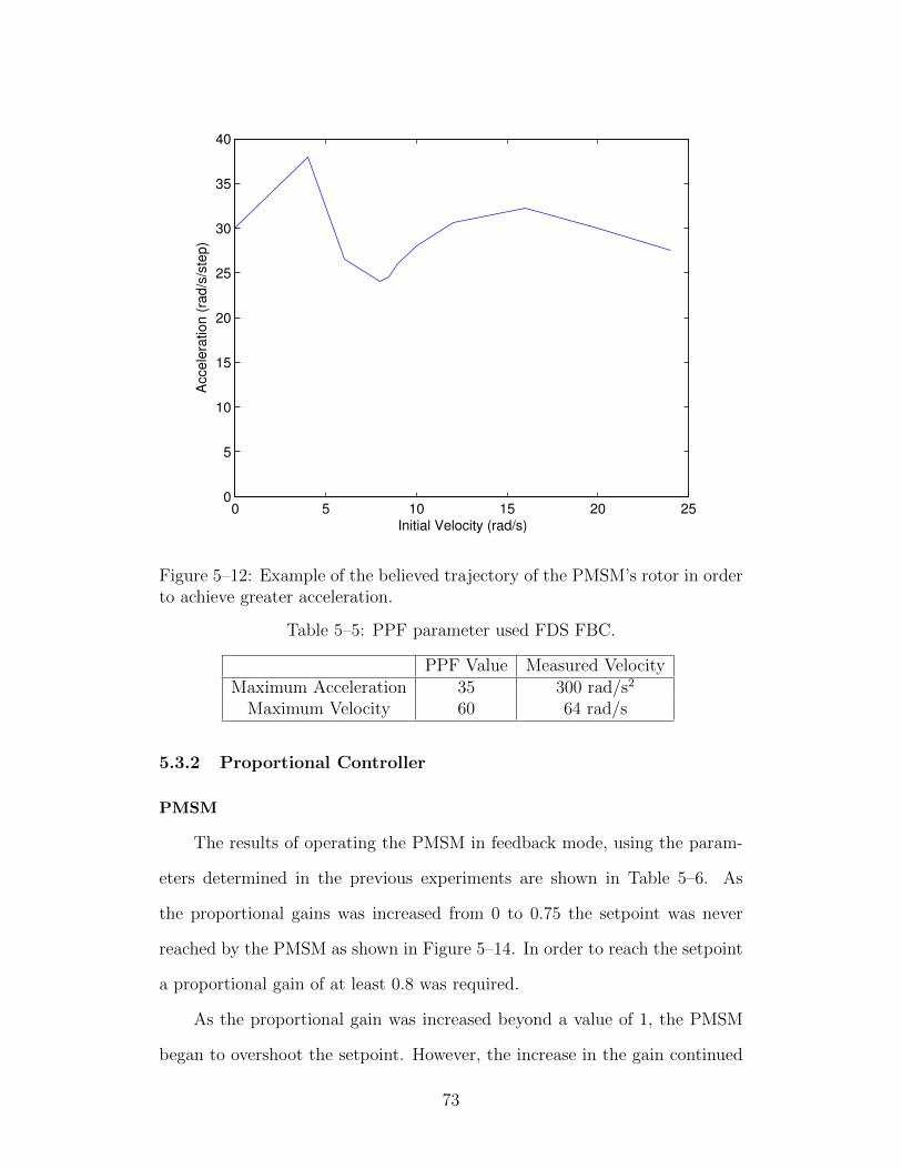
0 5 10 15 20 250
5
10
15
20
25
30
35
40
Initial Velocity (rad/s)
Acce
lera
tio
n (
rad
/s/s
tep
)
Figure 5–12: Example of the believed trajectory of the PMSM’s rotor in orderto achieve greater acceleration.
Table 5–5: PPF parameter used FDS FBC.
PPF Value Measured VelocityMaximum Acceleration 35 300 rad/s2
Maximum Velocity 60 64 rad/s
5.3.2 Proportional Controller
PMSM
The results of operating the PMSM in feedback mode, using the param-
eters determined in the previous experiments are shown in Table 5–6. As
the proportional gains was increased from 0 to 0.75 the setpoint was never
reached by the PMSM as shown in Figure 5–14. In order to reach the setpoint
a proportional gain of at least 0.8 was required.
As the proportional gain was increased beyond a value of 1, the PMSM
began to overshoot the setpoint. However, the increase in the gain continued
73

0 5 10 15 20 25 30 350
5
10
15
20
25
30
35
40
45
50
Initial Velocity (rad/s)
Acce
lera
tio
n (
rad
/s/s
tep
)
Figure 5–13: Results of FDS’s relationship between initial velocity and theacceleration.
to decrease the settling time. At a proportional gain of 10 the PMSM lost
synchronization and the PMSM stalls making any gain greater than 10 unsta-
ble. The instability is not a result of the maximum velocity and acceleration,
but the transient on the PMSM rotor and rapidly changing controller signal.
Decreasing the PPF’s parameters would allow the proportional gain to
increase; however, the response and performance of the PMSM would also de-
crease, thus, limiting the performance of the system. The PMSM performed
optimally at a gain of 7, having a settling time of 1.095 seconds.
FDS
The results of operating the FDS with a proportional controller are shown
in Table 5–7. The settling time performance was greater for the FDS because
74

Table 5–6: PMSM P Controller results.
Proportional Gain Tp Settling Time %overshoot Stable/Unstable0.8 NA 1.876 NA Stable1 NA 1.500 NA Stable
2.5 1.379 1.206 NA Stable3 1.278 1.175 NA Stable4 1.157 1.171 NA Stable5 1.130 1.122 NA Stable7 1.103 1.095 NA Stable10 1.080 1.059 NA Unstable
of the increased inertia the system had. The increased inertia resulted in a
damping effect, which caused the FDS to reach steady state faster and reduced
the amount of overshoot to zero for gains below 7. At a gain of 7 the FDS was
not unstable; however, the settling time of the FDS increased dramatically,
thus making the optial proportional gain for the FDS equal to 5.
Table 5–7: FDS Proportional controller results.
Proportional Gain Settling Time %Overshoot Stable/Unstable1 1.606 NA Stable
2.5 0.881 NA Stable3 0.758 NA Stable4 0.593 NA Stable5 0.519 NA Stable7 1.344 12% Marginally Stable10 1.429 22% Marginally Stable
5.3.3 Proportional Derivative Controller
PMSM
The results for multiple controller configuration can be found in Table
5–8. The added derivative terms for the PMSM did not improve performance
and caused the settling time to increase; however, as the gain was increased,
passed the stability limit of the PMSM’s proportional controller, the added
derivative controller resulted in decreased settling time then the proportional
75

0 5 10 15 200
10
20
30
40
50
60
Time (second)
Dis
pla
ce
me
nt(
radia
ns)
Figure 5–14: Results for PMSM displacement with proportional gain equal to0.3.
controller could achieve solely.
FDS
The results for the proportional derivative controller are shown in Table
5–9. The increased derivative gain resulted in an increased in settling time.
Unlike with the PMSM PD controller, the FDS remains stable for gain upto 10.
When Table 5–7 is compared to Table 5–9, it can be seen that there
is no advantage of running the system with a PD controller. The results
demonstrate how adding the derivative controller to the system causes the
settling time to increase. An increase in settling time means less performance
making the implementation of the PD controller on the FDS non beneficial.
76

Table 5–8: PMSM Proportional Derivative controller results.
Proportional Derivative Settling % Overshoot StableGain Gain Time Unstable
4 0.1 1.171 NA Stable4 1 1.190 NA Stable4 2 1.190 NA Stable4 5 1.204 NA Stable4 10 1.280 NA Stable4 30 NA NA Stable4 40 NA NA Unstable6 0.1 1.112 NA Stable6 1 1.112 NA Stable6 5 1.181 NA Stable6 10 1.259 NA Stable10 0.1 1.086 NA Stable10 1 1.091 NA Stable10 5 1.108 NA Stable10 10 1.110 NA Stable25 5 NA NA Unstable50 5 NA NA Unstable
Another observation comes from the fact that the method used to choose the
best controller.
77

Table 5–9: FDS Proportional Derivative controller results.
Proportional Derivative Settling %overshoot StableGain Gain Time Unstable
3 1 1.307 NA Stable3 2 1.324 NA Stable3 4 1.463 NA Stable3 10 1.487 NA Stable3 20 1.097 NA Stable7 1 1.115 NA Stable7 3 1.122 NA Stable7 6 1.122 NA Stable10 1 1.183 21% Stable10 5 1.085 NA Stable
78

CHAPTER 6CONCLUSION and FUTURE WORK
6.1 Conclusion
In this thesis, vibrations of a BSS were first reduced and experiments were
performed to measure some key parameters. It was concluded that the the
vibrations are caused by the PMSM operating at low velocities and the critical
velocity of the rotating ball screw. The critical velocity of the FDS was found
to be at a velocity of 74 rad/s, and the PMSM has a resonance frequency at
an operating velocity of 13 rad/s.
The models adapted from the literature identified the natural frequency of
the BSS to be 138 Hz and that of the PMSM 35 Hz. The resonant frequency of
the PMSM, also known as the resonant velocity, cannot be avoided unless the
controller sweeps over the velocity without quickly or through microstepping
the PMSM does not experience resonance and can function at all velocities.
The FDS including the motor drive system was designed and constructed
to validate the models as well as implementing feedback control. A PPF was
developed to allow the PMSM to be controlled with a signal input which
linearly correlates with the rotational velocity of the PMSM. The PPF is not
completely linear but is close enough for robust controllers, P and PD, to be
implemented.
The PPF was tuned for both the FDS and PMSM, having only a difference
of 9% for the maximum velocity and 25% difference for the acceleration. The
P and PD controller functioned using practically the same controller gains.
and PPF parameters, proving their robustness. The PD controller performed
79

better for operating the PMSM directly with no attached load because of the
low inertia of the shaft. The P controller outperformed that of the PD when
used on the FDS because of the damping effect caused by the addition of the
BSS.
6.2 Future Work
The following recommendation for future work are:
1. Investigate the effects of inertial loads on the system performance. Iden-
tification of the maximum velocity and acceleration for each load can
then be analyzed for a correlation.
2. Optimize the PPF by utilizing additional computations resources such
as microcontroller or PC. The increased computing power could allow
the performance of the linearization filter, PPF, to increase thus further
optimizing the PPF design.
80
REFERENCES
[1] C. E. Okwudire and Y. Altintas, “Hybrid modeling of ball screw driveswith coupled axial, torsional, and lateral dynamics,” Journal of Mechan-ical Design, vol. 131, no. 7, p. 071002, 2009.
[2] S. F, “Ball bearing screw and nut,” Nov. 10 1931. US Patent 1,831,080.
[3] M. Zaeh, T. Oertli, and J. Milberg, “Finite element modelling of ballscrew feed drive systems,” CIRP Annals-Manufacturing Technology,vol. 53, no. 1, pp. 289–292, 2004.
[4] C. Okwudire, Finite Element Modeling of Ballscrew Feed Drive Systemsfor Control Purposes. PhD thesis, University of British Columbia, 2005.
[5] Y. Liu, T. Zhao, and H. Zhang, “Hybrid dynamic modeling of a high-speed ball-screw drive system,” in Mechanic Automation and ControlEngineering (MACE), 2010 International Conference on, pp. 3049–3052,IEEE, 2010.
[6] Y. Zhou, F. Peng, and J. Chen, “Torsion vibration analysis of lead-screw feed drives with changeable table position and work-piece mass,”in Mechatronics and Automation, 2007. ICMA 2007. International Con-ference on, pp. 2194–2199, IEEE, 2007.
[7] K. Erkorkmaz and A. Kamalzadeh, “High bandwidth control of ball screwdrives,” CIRP Annals-Manufacturing Technology, vol. 55, no. 1, pp. 393–398, 2006.
[8] A. Kamalzadeh, Precision control of high speed ball screw drives. PhDthesis, University of Waterloo, 2008.
[9] M. Shams, M. Zarei-nejad, and M. Safdari, “Fuzzy sliding mode controlof a ball screw driven stage,” in Mechtronic and Embedded Systems andApplications, 2008. MESA 2008. IEEE/ASME International Conferenceon, pp. 369–374, IEEE, 2008.
[10] Y.-T. Shen, Y.-R. Hwang, and C.-S. Cheng, “A robust sliding mode con-troller design for a ball screw table driven by an air motor,” Journal ofmechanical science and technology, vol. 23, no. 11, pp. 3005–3012, 2009.
[11] Y. Li, J. Huo, X. Li, J. Wen, Y. Wang, and B. Shan, “An open-loop sinmicrostepping driver based on fpga and the co-simulation of modelsim and
81
82
simulink,” in 2010 International Conference on Computer, Mechatronics,Control and Electronic Engineering, vol. 6, pp. 223–227, 2010.
[12] A. Astarloa, U. Bidarte, A. Zuloaga, and I. de Alegria, “Reconfigurablemicrostepping control of stepper motors using fpga embedded ram,” inIndustrial Electronics Society, 2003. IECON’03. The 29th Annual Con-ference of the IEEE, vol. 3, pp. 2221–2226, IEEE, 2003.
[13] Z. Huang, L. Li, and D. Guo, “Design of stepping motor driving mod-ule for automatic microscope system,” in Anti-counterfeiting, Security,and Identification in Communication, 2009. ASID 2009. 3rd InternationalConference on, pp. 328–331, IEEE, 2009.
[14] C. Yodsanti and M. Konghirun, “Implementation of two-axis highly ac-curate position control of space-vector pwm based microstepping bipolardrive,” in Electrical Machines and Systems, 2008. ICEMS 2008. Interna-tional Conference on, pp. 1027–1031, IEEE, 2008.
[15] C. Shah, Sensorless Control of Stepper Motor Using Kalman Filter. PhDthesis, Cleveland State University, 2004.
[16] M. Bodson and J. Chiasson, “Application of nonlinear control methods tothe positioning of a permanent magnet stepper motor,” in Decision andControl, 1989., Proceedings of the 28th IEEE Conference on, pp. 531–532,IEEE, 1989.
[17] K.-H. Tsui, N. C. Cheung, and K.-W. Yuen, “Novel modeling and damp-ing technique for hybrid stepper motor,” Industrial Electronics, IEEETransactions on, vol. 56, no. 1, pp. 202–211, 2009.
[18] A. Morar, “Stepper motor model for dynamic simulation,” ActaElec-trotehnica, vol. 44, no. 2, pp. 117–122, 2003.
[19] J.-J. Sinou and L. Jzquel, “Mode coupling instability in friction-inducedvibrations and its dependency on system parameters including damping,”European Journal of Mechanics - A/Solids, vol. 26, no. 1, pp. 106 – 122,2007.
[20] S. Frey, A. Dadalau, and A. Verl, “Expedient modeling of ball screw feeddrives,” Production Engineering, vol. 6, no. 2, pp. 205–211, 2012.
[21] J. Z. Sobolewski, “Vibration of the ball screw drive,” Engineering FailureAnalysis, vol. 24, pp. 1–8, 2012.
[22] S. Fukada, B. Fang, and A. Shigeno, “Experimental analysis and simula-tion of nonlinear microscopic behavior of ball screw mechanism for ultra-precision positioning,” Precision Engineering, vol. 35, no. 4, pp. 650–668,2011.

83
[23] C. C. Wei, J. F. Lin, and J.-H. Horng, “Analysis of a ball screw witha preload and lubrication,” Tribology International, vol. 42, no. 11,pp. 1816–1831, 2009.
[24] D. Olaru, G. C. Puiu, L. C. Balan, and V. Puiu, “A new model to estimatefriction torque in a ball screw system,” in Product Engineering, pp. 333–346, Springer, 2005.
[25] M. Zribi and J. Chiasson, “Position control of a pm stepper motor byexact linearization,” Automatic Control, IEEE Transactions on, vol. 36,no. 5, pp. 620–625, 1991.
[26] J. Gautheron, “Power supply with chopping circuit,” May 24 1977. USPatent 4,025,862.

APPENDIX ACode
84

%%%This script is designed to take a single phase from a stepper motor with %%%out the torque constant. If this works the next step is to turn it into %%%a function this way it can be used to simulate multiple phases, while %%%still having control of the pulse generator. This script will import %%%other functions for generating the pulses.
clear all; clear; clc;
%%%System: V(t) = emf(w) + R*I(t) +L*dI(t)/dt
%%%Controller Parameters %E = setpoint-position;
%%%Constants R = 0.24; %Ohms L = 0.0015; %H - Henrys emf = 0; %V - Volts km = 2.4/4.5; %Torque Constant Jm = 1.5e-3; %Inertia J_s = 0.15; %Inertia of Screw n = 50; %Steps pre rev/4 this is the amount of teeth Cm = .01; %Damping Parameter
% Example: Euler's method for dI/dt = (1/L)*(V(t) - I(t)*R) V_g = 24; %represents the scaler multiple to increase input voltage dt = 0.0001;
M = 1; C_b = 10; K = 1e5; J_s = 15708; %kg*mm^2; C_s = 1e3; K_s = 1e5; zeta = .95; L_s = .02; %Lead of Screw in m
Conv = (2*pi())/L_s;
%%%Lambda represents the wave length of the pulse being sent to the phases %%%of the stepper motor. Since the control of these pulse is ultimately %%%what will control the velocity of the stepper motor, the PD controller %%%will eventually be the control over the wavelength.
%lamda = [0.1:-0.01:0.01];%(1:-.5:.5); %lamda2 = [0.01:0.01:.1]; %lamda = [lamda1 lamda2]; % for k = 1:10 % lamda(k) = 1;

function [ pulse ] = squareWaveFun( waveLength, dt, ON )
if ON==1 signal_length = waveLength; % length of signal in seconds amplitude = 1; % amplitude of wave %dt = 1e-10; % time increment in seconds time = 0:dt:signal_length-dt; % time samples in seconds % Define the rectangle signal timeseries pulse = sign(sin(2*pi*time/waveLength)).*ones(size(time))*amplitude; % Plot the timeseries %plot(time,pulse,'r-'); else signal_length = waveLength; amplitude = 0; time = 0:dt:signal_length-dt; pulse = sign(sin(2*pi*time/waveLength)).*ones(size(time))*amplitude;
end

%%%This script is designed to simulate the ball screw system and solve the %%%problem numerically. It eill take the exact models found within my %%%thesis just for the the BSS. The final idea may be to turn the BSS into %%%a function which can be called by the higher level overall simulater to %%%call upon.
clear clc clear all
%%%For simplicity Resaons the nut will be dervied first %%%F = M*d2xdt2+C*dxdt+K*x
M = 1; C_b = 10; K = 1e5; J_s = 15708; %kg*mm^2; C_s = 1e3; K_s = 1e5; zeta = .95; L = .02; %Lead of Screw in m
Conv = (2*pi())/L;
%%%Outputs theta_s = []; omega_s = []; alpha_s = []; x = []; v = []; a = [];
%%%Inputs Tau = 1e6; %Nmm for i=1:500000 Tau1(i) = 1e6; end for i=1:500000-1 Tau2(i) = 0; end Tau = [Tau1 Tau2];
%%%Initial Conditions theta_s(1) = 0; omega_s(1) = 0; %alpha_s(1) = 0; x(1) = 0; v(1) = 0; %a(1) = 0; x_test(1)=0; F(1) = 0;
%%%Timing Variables t = 100; %time of simulation in seconds

#include <Wire.h>
byte data[2]; byte* a; int test = 100; //unsigned int b[13] = 32769, 65535, 0 , 32769 , 39322 , 26214 , 45876 ,
19661, 52429 , 13107, 58984, 6555, 32768; //unsigned int b[8] = 32769, 65535 , 0 , 65535 , 0 , 65535 , 0 , 32769;
unsigned int z = 0; unsigned int b = z + 32768;
void setup() Wire.begin(4); Serial.begin(9600); long t=0; long t2; void loop()
t = micros(); userInput();
//delay(3000);
//for( int i = 0;i<sizeof(b)/2;i++ )
//byte* c = (byte*) &b[i]; byte* c = (byte*) &b; Serial.println(b); Wire.beginTransmission(4); // transmit to device #4 Wire.write( c , 2 ); // sends one byte Wire.endTransmission(); int p = 10000-(micros()-t); delayMicroseconds(p); //Serial.println(10000-(micros()-t)); //Serial.println(p); //
void userInput() if ( Serial.available() > 0 ) z = Serial.parseInt(); //z = linearTransformation(z); b = (unsigned int) (z + 32768); else b = b; //delay(20);

#include <Wire.h>
const int stepPin = 10; //white const int dirPin = 11; //brown const int disablePin = 12; //blue
//Stepper myStepper( stepsPerRevolution, 8,9,10,11 ); //StepperMotor Variables float input; float inputA; float rate; float start; float end; long stepperPulse; float C; float accLimiter;
//I2C Communication Variables byte i2CPort[2];
void setup()
//Serial.begin(115200);
Wire.begin(4); // join i2c bus with address #4 Wire.onReceive(receiveEvent); // register event
pinMode( stepPin, OUTPUT ); pinMode( dirPin, OUTPUT ); pinMode( disablePin, OUTPUT );
digitalWrite( disablePin,HIGH ); delay(500); digitalWrite( disablePin,LOW );
//User Inputs C = 75; accLimiter = 25;
//Initial Values input = 0; inputA = 0; start = 0; end = 0; stepperPulse = 0;
void loop()
updateMemory( &start, &end, &rate, &input, &inputA );

#include <Wire.h>
byte data[2];
byte* a;
int test = 100;
//unsigned int b[13] = 32769, 65535, 0 , 32769 , 39322 , 26214 , 45876 ,
19661, 52429 , 13107, 58984, 6555, 32768;
//unsigned int b[8] = 32769, 65535 , 0 , 65535 , 0 , 65535 , 0 , 32769;
unsigned int z = 0;
unsigned int b = z + 32768;
void setup()
Wire.begin(4);
Serial.begin(9600);
long t=0;
long t2;
void loop()
t = micros();
userInput();
//delay(3000);
//for( int i = 0;i<sizeof(b)/2;i++ )
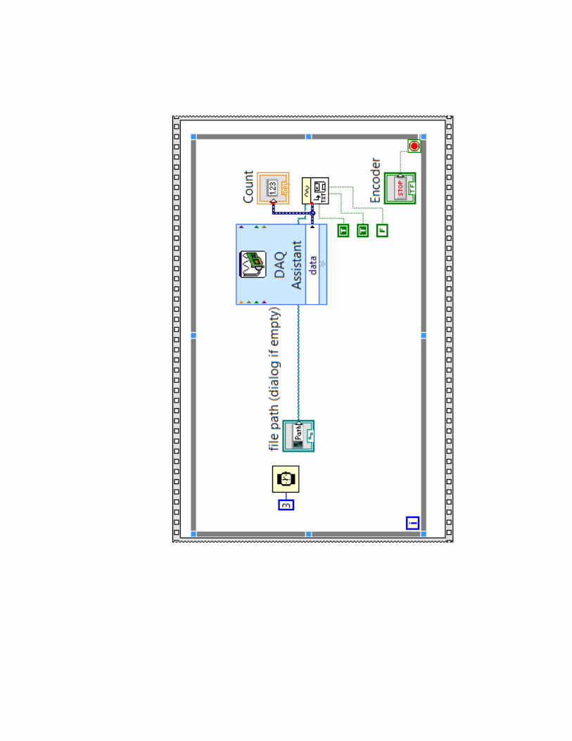

APPENDIX BDesign
92


APPENDIX CData Sheets
97

TB6560AHQ/AFG
2011-01-18 1
TOSHIBA BiCD Integrated Circuit Silicon Monolithic
TB6560AHQ, TB6560AFG PWM Chopper-Type Bipolar Driver IC for Stepping Motor Control
The TB6560AHQ/AFG is a PWM chopper-type stepping motor driver IC designed for sinusoidal-input microstep control of bipolar stepping motors. The TB6560AHQ/AFG can be used in applications that require 2-phase, 1-2-phase, 2W1-2-phase and 4W1-2-phase excitation modes. The TB6560AHQ/AFG is capable of low-vibration, high-performance forward and reverse driving of a two-phase bipolar stepping motor using only a clock signal.
Features • Single-chip motor driver for sinusoidal microstep control of
stepping motors • High output withstand voltage due to the use of BiCD process:
Ron (upper and lower sum) = TB6560AHQ: 0.6 Ω (typ.) TB6560AFG: 0.7 Ω (typ.)
• Forward and reverse rotation • Selectable phase excitation modes (2, 1-2, 2W1-2 and 4W1-2) • High output withstand voltage: VDSS = 40 V • High output current: IOUT = TB6560AHQ: 3.5 A (peak)
TB6560AFG: 2.5 A (peak) • Packages: HZIP25-P-1.27
HQFP64-P-1010-0.50 • Internal pull-down resistors on inputs: 100 kΩ (typ.) • Output monitor pin: MO current (IMO (max) = 1 mA) • Reset and enable pins • Thermal shutdown (TSD)
*: These ICs are highly sensitive to electrostatic discharge. When handling them, ensure that the environment is protected against electrostatic discharge. Ensure also that the ambient temperature and relative humidity are maintained at reasonable level.
TB6560AHQ
TB6560AFG
Weight HZIP25-P-1.27: 9.86 g (typ.) HQFP64-P-1010-0.50: 0.26 g (typ.)
*Solderability 1. Use of Sn-37Pb solder bath
*solder bath temperature = 230°C *dipping time = 5 seconds *number of times = once *use of R-type flux
2. Use of Sn-3.0Ag-0.5Cu solder bath *solder bath temperature = 245°C *dipping time = 5 seconds *the number of times = once *use of R-type flux

Warning:1、 ! 6560
.2、
、
Check the connection twice The Tbchipset can be damaged if the motor or thepower supply are not connected properlyDont apply a motor that its rated currentis more than 3A to this driver.
3 Do not set the current more than the motorrated current!
Tb6560 stepping motor driver V20
Photocouplers
Running Current
( )A 0.3 0.5 0.8 1 1.1 1.2 1.4 1.5 1.6 1.9 2 2.2 2.6 3
SW1 OFF OFF OFF OFF OFF ON OFF ON ON ON ON ON ON ON
SW2 OFF OFF ON ON ON OFF ON OFF OFF ON OFF ON ON ON
SW3 ON ON OFF OFF ON OFF ON ON OFF OFF ON ON OFF ON
S1 ON OFF ON OFF ON ON OFF ON OFF ON OFF ON OFF OFF
Stop Current
S2
20% ON
50% OFF
Excitation Mode
S3 S4
whole OFF OFF
half ON OFF
1/8 ON ON
1/16 OFF ON
Decay Setting
S5 S6
0% OFF OFF
25% ON OFF
50% OFF ON
100% ON ON
、 ,
、 ,
、
、
2 5V
3 CLK
4
CW5 EN
The normal input voltage is if it is more than 5V,than a series resistoris needed. this resistance is 1K case 12V and 2.4K case 24V.when pulse is applied to the stepping motor will rotate,and stop when there is none,and the motor driver will change its currentto the half mode as setting to hold the motor still.
Motor rotate clockwise when is low level and counterclockwise when
is high level.Motor is enable when is low level and disable when EN is high leve.
CW
1、 , 。6 input terminals can be connected as common anode or cathode
current
Note:
Step
Wiring Terminal symbol Description
+24V,GND Power positive and negative
A+,A- Motor phase A
B+,B- Motor phase B
CLK+,CLK- Pulse positive and negative
CW+,CW- Direction positive and negative
EN+,EN- Enable positive and negative