Embed Size (px)
Citation preview
Simulation and analysis of an individual-based model forgraph-structured plant dynamicsI
F. Campillo1,∗, N. Champagnat2
Abstract
We propose a stochastic individual-based model of graph-structured population, viewed
as a simple model of clonal plants. The dynamics is modeled in continuous time and
space, and focuses on the effects of the network structure of the plant on the growth
strategy of ramets. This model is coupled with an explicit advection-diffusion dynamics
for resources. After giving a simulation scheme of the model, the capacity of the model
to reproduce specific features of clonal plants, such as their efficiency to forage resources
and colonize an empty field by means of phalanx or guerrilla strategies, is numerically
studied. Next, we propose a large population approximation of the model for phalanx-
type populations, taking the form of an advection-diffusion partial differential equation
for population densities, where the influence of the local graph structure of the plant
takes the form of a nonlinear dependence in the gradient of resources.
Keywords: Markov process, individual-based model (IBM), clonal plant, asymptotic
analysis
1. Introduction
Individual-based models (IBMs) are in constant development in computational ecol-
ogy (DeAngelis and Gross, 1992; Dieckmann et al., 2000; Grimm and Railsback, 2005).
IThis work received support by the French national research agency (ANR) within the SYSCOMMproject ANR-08-SYSC-012.
∗Corresponding authorEmail addresses: [email protected] (F. Campillo), [email protected]
(N. Champagnat)1Address: MODEMIC project-team, INRIA/INRA, UMR MISTEA, 2 place Viala, 34060 Montpellier
Cedex 01, France.2Address: TOSCA project-team, INRIA Nancy – Grand Est, IECN, UMR 7502, Nancy-Universite,
Campus Scientifique, B.P. 70239, 54506 Vandœuvre-les-Nancy Cedex, France.
Preprint submitted to Ecological Modelling February 27, 2012
These models aim to represent the dynamics of populations, and in contrast with con-
ventional models where the population is represented as an aggregate state such as the
population size or the total biomass, they explicitly describe each individual as well as
each mechanism acting on these individuals. In this sense, conventional models corre-
spond to a macroscopic approach and IBMs to a microscopic one. Such a description
of an ecosystem at the scale of the individual usually rely on stochastic mechanisms
reflecting the interactions of the individual with its neighbors and its environment.
Among plant communities, those involving a clonal reproduction constitute an inter-
esting challenge in terms of modeling. In most clonal plants, growth can be processed hor-
izontally via the development of modified stems, rhizomes or stolons, connecting ramets
(Van Groenendael et al., 1996). Ramets are potentially autonomous new individuals and
possess aerial and belowground organs in order to sample and uptake resources, like wa-
ter, light, organic nutrients, nitrates or phosphorus (Van Groenendael et al., 1996; Klimes
et al., 1997). This network structure provides the ability to colonize space (Harper, 1981;
Hutchings, 1999), and allows the exchange of resources and information (Marshall, 1990;
Stuefer et al., 2004; Wijesinghe and Hutchings, 1997; Hutchings, 1999; Charpentier and
Stuefer, 1999; Klimes et al., 1997). In particular, this network structure implies strong
spatial constraints to the architecture of a clonal plant network that have tradition-
ally been classified along a gradient from phalanx to guerrilla strategies (Lovett-Doust,
1981). Phalanx strategies comprise clonal plants with dense network structures with
short spacers and resulting in an interrupted front of aggregated ramets with a slow ra-
dial propagation (Cheplick, 1997; Humphrey and Pike, 1998). On the contrary, guerrilla
strategies produce long and poorly ramified connections which favor space colonization.
The graph structure allows clonal plants to colonize space in order to locate the
most favorable areas in terms of resources (spatial colonization sensu Wildova et al.,
2007), and exploit the resources in these sites in order to favor the growth of new ramets
(potential descendants) in these areas (space occupation sensu Wildova et al., 2007).
Spatial structure of the interacting species should be therefore a key element of the
dynamics of plant communities.
IBMs generate spatial patterns and dynamics at the scale of plant communities from
local interactions between individuals, which are the processes involved in real commu-
2

nities. A sound model in plant ecology should be spatial and individually based. Two
main categories of IBMs can be distinguished: “realistic IBMs” which take into account
a large number of mechanisms, and “simple IBMs” which focus on a specific feature of
the ecosystem and neglect the others. The first category of models aims for realistic local
population structure, whereas the second category can be used to study the influence of
a specific feature of the ecosystem on large spatial scales.
For clonal plants, almost all the IBMs studied in the literature belong to the “real-
istic” category. Most of them are developed on spatial grids (square of hexagonal, for
example), representing the possible locations of each element of the plant (Dieckmann
et al., 1999; Kun and Oborny, 2003; Oborny, 1994; Oborny et al., 2000, 2001; Oborny
and Kun, 2002; Winkler and Klotz, 1997; Winkler et al., 1999; Winkler and Fischer,
2002; Winkler and Stocklin, 2002). Some models also rely on continuous space domains,
where individuals or plant elements can be located at any place in space (Herben and
Suzuki, 2002; Herben and Novoplansky, 2008). They belong to a larger class of mod-
els, well developed in the more general context of Plant Ecology (Bolker and Pacala,
1999; Dieckmann et al., 1999, 2000; Brown and Bolker, 2004; Bolker, 2004; Fournier and
Meleard, 2004; Birch and Young, 2006). Many of these models belong to the class of
simple models, because simple IBMs in continuous space and time are within the scope
of numerical and mathematical analysis on large spatial scales, whereas IBMs on grids
are much harder to study mathematically. These models have originally been developed
and studied for adaptive dynamics in evolutionary biology, where plants locations are re-
placed by individuals’ phenotypic quantitative characters (Metz et al., 1996; Dieckmann
and Law, 1996; Champagnat et al., 2006; Meleard and Tran, 2009; Champagnat and
Meleard, 2011).
IBMs are useful for studying local structures in plant communities, e.g. for devel-
opment or behavioral studies. However, they are of little practical help for studies at
the scale of a field, where one could want to study the competitive exclusion or coex-
istence of species (Bolker and Pacala, 1999), or simply compute long time statistics of
the model, like the mean, equilibrium relative abundance of species. A proficient answer
to such questions typically requires us to combine statistical and large time numerical
studies, and are hence out of reach of an IBM using usual numerical power (Mony et al.,
3

linksnodes
Figure 1: The plant is represented as a set of nodes connected by links. The nodes can be seen as ramets
and the links as rhizomes.
2012). For such problems, one typically uses partial differential equation (PDE) models
(El Hamidi et al., 2012), but usually no aspect of the local architecture of the plants is
included in the PDE.
The aim of this work is to construct a simple IBM in continuous space and time
for clonal plants, which can be numerically and mathematically studied at the scale of
a grassland, and which can make the link between realistic IBMs and PDE models on
large scales.
We chose to construct an IBM which focuses on the influence of the graph on the
horizontal growth strategy (rate of creation of new connections, new ramets, and the
location of new ramets) through a stochastic IBM in continuous time and space, coupled
with the graph structure of the plant. In view of the crucial influence of resources
exchange between ramets on the space colonization and the localization of favorable
areas, we couple our IBM with resources distributed over continuous space, following an
advection- diffusion deterministic dynamics. This model is tested in the framework of the
phalanx-guerrilla continuum of growth strategies, and we provide exact large population
approximations as partial differential equations for the local population density.
2. Dynamics of the plant and of the resources
At time t the clonal plant is represented as a set of nodes (ramets) that may be
connected by links (rhizomes or stolons), see Figure 1. In this simplified representation
of a clonal plant, ramets are represented by points in the plane, and connection by
straight lines between two ramets. All ramets and connections are assumed to be identical
4

in terms of demographic parameters and resource consumption. Age and growth are
neglected, and connections do not uptake resources or incorporate biomass. The influence
of other above ground and below ground aspects of the plant are not physically modelled.
They are only expressed through the birth and death parameters and the interaction with
resources described below.
The state of the nodes is described by the following finite measure:
νt =Nt∑i=1
δxit (1)
where xit ∈ R2 is position of the ith node and Nt total number of nodes; δx denotes
the Dirac measure centered on the point x. The measure νt describes the distribution
of nodes over the space D ⊂ R2 of spatial positions. We consider for simplicity D =
[x(1)min, x
(1)max] × [x(2)
min, x(2)max]. The measure νt is a counting measure: νt(D) is the total
number Nt of individuals and, for all subdomain B of D, νt(B) =∑Nti=1 1B(xit) is the
number of individuals in B.
For any node at position x we define the set of indices of the nodes connected to x:
J(t, x) ={i = 1 · · ·Nt ; x and xit are connected
}. (2)
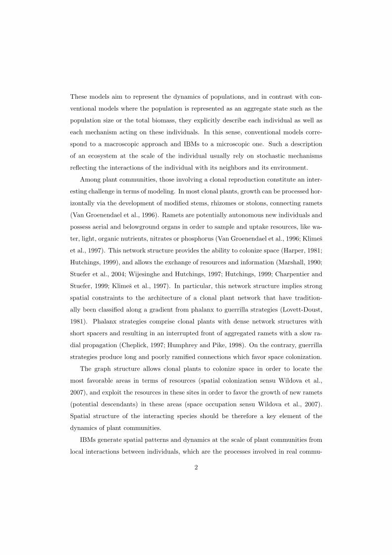
The plant grows in a resource landscape (see Figure 3). At each time t, this resource
landscape is represented by r(t, x) ∈ [0, rmax] the available resources at position x ∈ D.
The nodes accessing high levels of resources r(t, x) are more likely to give birth to new
nodes.
Birth and death rates
Each node of νt in position x may disappear at a death rate µ(t, x) and give birth to
a new node at a birth rate λ(t, x). These rates are per capita rates. Global death and
birth rates at population level are respectively:
λt =Nt∑i=1
λ(t, xit) , µt =Nt∑i=1
µ(t, xit) . (3a)
The global event rate is:
µt + λt . (3b)
5
Champagnat et al., 2006; Champagnat and Meleard, 2007;Meleard and Tran, 2009; Champagnat and Meleard, 2010)or for competition-colonization in population ecology (Bolkerand Pacala, 1997, 1999; Dieckmann et al., 1999, 2000;Dieckmann and Law, 2000; Law and Dieckmann, 2000;Fournier and Meleard, 2004; Birch and Young, 2006).
Our goal is to construct and analyze a “simple IBM”putting emphasis on one of the main features of clonalplants, believed to confer them an advantage for resourceexploitation and space colonization—their network struc-ture and the transfer of information and resources throughrhizomes or stolons. This graph structure allows clonalplants to localize favorable areas in terms of resources (Bell,1984, foraging), and can favor the growth of new rametsin these areas (Roiloa and Retuerto, 2006). This bothallows a better prospection of resources like water, light,organic or inorganic nutrients, and a better survival of de-scendants. In addition, ramets are able to share resourcesthrough links in the network (Stuefer et al., 2004; Wi-jesinghe and Hutchings, 1997; Hutchings, 1999, physiolog-ical integration). In particular, ramets located in areaswith few resources can benefit from resources stored byramets located in richer areas, transmitted through con-nections between ramets. In addition, translocation be-tween ramets also allows clonal plants to resist to otherstresses, like mechanical stress (Yu et al., 2008) or par-asitism (D’Hertefeldt and van der Putten, 1998). Themodel we study here concentrates on these phenomenaand their influence on the reproductive strategy. In par-ticular, several other known features of clonal plants arenot modeled, e.g. the specialization of ramets (Charpen-tier and Stuefer, 1999), the resource storage in rhizomesor stolons (Klimes et al., 1997), or the effects of the graphstructure on the growth of ramets and rhizomes or stolons.
The paper is organized as follows. In Section 2, we de-scribe the stochastic individual-based model, coupled withthe graph structure of the plant and a piecewise deter-ministic advection-diffusion model for resources. In Sec-tion 3, a partially “exact” Monte Carlo simulation schemeis described. Simulation results are discussed in Section 4.Large population approximations of the population arethen given in Section 5. Finally, several extensions of ourmodel are discussed in Section 6.
2. Dynamics of the plant and of the resources
At time t the clonal plant is represented as a set ofnodes (ramets) that may be connected by links (rhizomesor stolons), see Figure 1. The state of the nodes is de-scribed by the following finite measure:
νt =Nt�i=1
δxit
(1)
where xit ∈ R2 is position of the ith node and Nt to-
tal number of nodes; δx denotes the Dirac measure giv-ing mass 1 to the point x. The measure νt describes
linksnodes
Figure 1: The plant is represented as a set of nodes connected bylinks. The nodes can be seen as ramets and the links as rhizomes.
3.5 4 4.5 5 5.51
1.2
1.4
1.6
1.8
2
2.2
2.4
2.6
2.8
3
3.5 4 4.5 5 5.51
1.2
1.4
1.6
1.8
2
2.2
2.4
2.6
2.8
3
3.5 4 4.5 5 5.51
1.2
1.4
1.6
1.8
2
2.2
2.4
2.6
2.8
3
t1 t2 t3
3.5 4 4.5 5 5.51
1.2
1.4
1.6
1.8
2
2.2
2.4
2.6
2.8
3
3.5 4 4.5 5 5.51
1.2
1.4
1.6
1.8
2
2.2
2.4
2.6
2.8
3
t4 t5
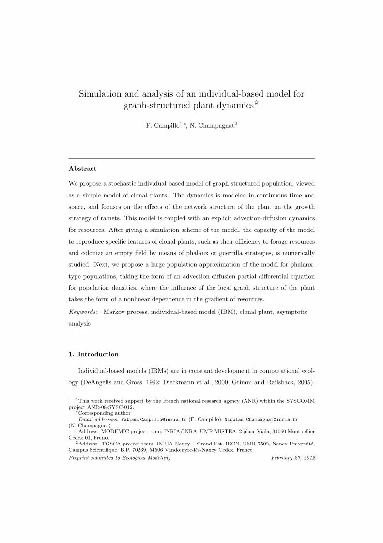
Figure 2: The nodes evolves in a resource landscape (black/white:high/low resource availability). The nodes accessing high levels ofresources are more likely to give birth to new nodes ( t1 → t2 →t3). Simultaneously the node and the link between this node andthe mother node are created. When a node disappears all the linksconnected with it simultaneously disappear ( t3 → t4).
the distribution of nodes over the space D ⊂ R2 of spa-tial positions. In this article, we consider for simplicityD = [x(1)
min, x(1)max]×[x(2)
min, x(2)max]. The measure νt is a count-
ing measure: the total mass νt(D) is the number Nt ofindividuals and νt(B) is the number of individuals in thesubdomain B of D.
For any node at position x we define the set of indicesof the nodes connected to x:
J(t, x) =�i = 1 · · ·Nt ; x and xi
t are connected�
. (2)
Note that the basic entities of our IBM are ramets and con-nections. In particular, we do not account for the growth oframets and rhizomes or stolons (except through the birthand death mechanisms described below).
The plant evolves in a resource landscape (see Figure3). At each time t, this resource landscape is representedby r(t, x) ∈ [0, rmax] the available resources at positionx ∈ D. The nodes accessing high levels of resources r(t, x)are more likely to give birth to new nodes.
First we describe the rates at which nodes disappearand give birth to new individuals, then we describe thedispersion kernel, and finally the dynamics of the resource.
2
Figure 2: The nodes evolve in a resource landscape (black/white: high/low resource availability). The
nodes accessing high levels of resources are more likely to give birth to new nodes ( t1 → t2 → t3).
Simultaneously the node and the link between this node and the mother node are created. When a node
disappears all the links connected with it simultaneously disappear ( t3 → t4).
0 2 4 6 8 100
1
2
3
4
5
6
7
8
9
10
Figure 3: Snapshot of the resource landscape r(t, x) ∈ [0, rmax] at a given time t. The resource dynamics
is modeled as an advection/diffusion transport equation (10) in interaction with the dynamics of the
nodes.
6

Basically, the per capita rates depend on the local availability of resources: we suppose
that the birth rate λ(t, x) is an increasing function of r(t, x) and the death rate is a
decreasing function of r(t, x). For example:
λ(t, x) = 1{|J(t,x)|≤Nmax}(λ0 + λ1 r(t, x)
), (4a)
µ(t, x) = µ0 + µ1 [rmax − r(t, x)] (4b)
where |J(t, x)| is the cardinal of the set J(t, x) and Nmax is the maximum number of con-
nections per node. In IBMs on hexagonal grids, one usually has Nmax = 6 or sometimes
less (for example, a ramet never has more than 3 connections in Oborny and Englert,
2012). Note that the continuous space formalism does not require any restriction on the
number of connections from a ramet (one could take Nmax = +∞). This would lead to
more realistic graph structures for sympodial species which display several buds develop-
ing from a ramet. Note that the local limitation of resources due to ramet consumption
(see below) prevents an excessive local growth of the number of connections and ramets
similar to competition processes between plants, and hence implicitely impose a limit on
the number of neighbors of each ramet.
When a node is added to the population, it is always linked with the mother node,
and the set of connections J(t, xit) corresponding to the mother node and the new node
are modified accordingly. In addition, when a node x is removed from population, all
connections to x are suppressed from all the sets J(t, xit) (see Figure 2).
Dispersion kernel
We have chosen to focus on the effects of the graph structure of the plant on its
horizontal growth strategy, and for simplicity, only on the choice of the position of a new
ramet relative to its “father ramet”, also called dispersion kernel.
A node at position x at time t gives birth to a new node at position y = x + v
according to the p.d.f. Dt,x(v). We propose the following distribution:
Dt,x(v) = f(κ, (dt,x, v)) g(‖v‖) (5)
where
7

0 2 4 6 8 100
1
2
3
4
5
6
7
8
9
10
Figure 3: Snapshot of the resource landscape r(t, x) ∈ [0, rmax] ata given time t. The resource dynamics is modeled as an advec-tion/diffusion transport equation (9) in interaction with the dynam-ics of the nodes.
Birth and death ratesEach node of νt in position x may disappear at a death
rate µ(t, x) and give birth to a new node at a birth rateλ(t, x). These rates are per capita rates. Global death andbirth rates at population level are respectively:
λt =Nt�i=1
λ(t, xit) , µt =
Nt�i=1
µ(t, xit) . (3a)
The global event rate is:
κt = µt + λt . (3b)
Basically, the per capita rates depend on the local avail-ability of resources: we suppose that the birth rate λ(t, x)is an increasing function of r(t, x) and the death rate isdecreasing function of r(t, x). For example:
λ(t, x) = λ0 + λ1 r(t, x) ,
µ(t, x) = µ0 + µ1 [rmax − r(t, x)] .(4)
These rates may account for many other mechanisms. Onecan limit the number of connections per node with thefollowing birth rate:
λ(t, x) = 1{|J(t,x)|≤Nmax} [λ0 + λ1 r(t, x)] . (5)
where |J(t, x)| is the cardinal of the set J(t, x) and Nmax isthe maximum number of connections per node. One canalso account for the fact that resources can be translocatedthrough connections. A possibility could be to includea dependence of λ with respect to the incoming flux ofresources in the ramet, given by�
i∈J(t,x)
(r(t, xit)− r(x)). (6)
(See also the discussion below.)
θ
g(|v|)
reference direction
node x
new node x + v
dt,xf(κ, θ)
−3 −2 −1 0 1 2 3
0,5
1
1,5
2
2,5new shoot angle p.d.f.
radians
p.d.
f.
f(κ, θ)
0 0.1 0.2 0.3 0.4 0.50
5
10
15new shoot lenght p.d.f.
(m)
leng
th p
.d.f.
g(�v�)
Figure 4: The dispersion kernel (7) is the product of the angle prob-ability density function f and the length probability density functiong. When �dt,x� = 0 then we can for example choose f(θ) = 1
2π(uniform distribution).
When a node is added to the population, it is alwayslinked with the mother node, and the set of connectionsJ(t, xi
t) corresponding to the mother node and the newnode are modified accordingly. In addition, when a nodex is removed from population, all connections to x aresuppressed from all the sets J(t, xi
t) (see Figure 2).
Dispersion kernelA node at position x at time t gives birth to a new
node at position y = x+ v according to the p.d.f. Dt,x(v).We propose the following distribution:
Dt,x(v) = f(�dt,x�, (dt,x, v)) g(�v�) (7)
where
(i) (dt,x, v) is the angle between a preferred direction ofreference dt,x and the direction of the new shoot v,f(a, θ) is a p.d.f. on [−π, π) for all a ≥ 0;
(ii) g(�v�) is the p.d.f. on the length �v� of the connec-tion (see Figure 4).
For f(a, θ) we can choose the Von Mises distributionwith a parameter that may depend on a or, if no direc-tion is preferred, the uniform distribution. In this lastcase, Dt,x(v) ∝ g(�v�). Note that, in the case wherethe preferred direction dt,x is 0, the angle (dt,x, v) is un-defined, so one should take the uniform distribution, i.e.f(0, θ) = 1/2π. For g(�v�), if we want to fix the length ofthe connection to �0 then we just let Dt,x(v) = δ�0 (�v�).
For the preferred direction of reference dt,x, we needto account for the fact that the ramet can “perceive” theresource map from the connections with other ramets, forexample because of resource translocations. One possiblechoice for dt,x is:
dt,x =1
|J(t, x)|�
i∈J(t,x)
r(t, xit)− r(t, x)
|xit − x|2 [xi
t − x]. (8)
3
Figure 4: The dispersion kernel (5) is the product of the angle probability density function f , the Von
Mises distribution, and the length probability density function g, the log-normal distribution.
(i) (dt,x, v) is the angle between a preferred “direction of reference” dt,x and the di-
rection of the new shoot v, f(κ, θ) is a p.d.f. on [−π, π) centered on the angle 0
and with concentration parameter κ. For f we choose the Von Mises distribution
(circular normal distribution) with location parameter 0 and a given concentra-
tion parameter. The concentration parameter may depend on ‖dt,x‖ and when
‖dt,x‖ = 0, f is chosen as the uniform distribution, i.e. κ = 0.
(ii) g(‖v‖) is the p.d.f. on the length ‖v‖ of the connection (see Figure 4); g is chosen
as the log-normal distribution.
The preferred direction of reference should capture the effect of the local graph struc-
ture of the plant on its horizontal growth. Through their foraging ability, plants are
able to explore space and preferentially develop ramets in favorable sites (Van Kleunen
and Fischer, 2001), resulting in a preferential directional growth. Such sites could be
here sites with the lowest densities of ramets (competitive avoidance sensu Novoplansky,
2009) or sites with the highest resource level. In our model, we assume that growth
takes place preferentially in the direction of higher resource level. However, since our
model couples plants and resources dynamics, areas with high resource densities and low
density of ramets are actually implicitely correlated.
The information about the spatial location of the neighbors of a node at position x8
at time t can be summarized by the vector
1|J(t, x)|
∑i∈J(t,x)
xit − x|xit − x|
. (6)
When there is single neighbor, this vector gives the direction of the connection between
the ramets and its “mother ramet”. When there are more neighbors, this is simply
the mean vector of the directions of each connections leaving the ramet. If one wants to
model a preferred direction of growth in unexplored directions, one should favor dispersal
in the opposite direction of this vector.
The information about the resource flow entering the ramet at x through connections
can be summarized by the (positive or negative) number
1|J(t, x)|
∑i∈J(t,x)
[r(t, xit)− r(t, x)]. (7)
This formula assumes that the flow of resources in a connection is proportional to the
resource difference between the two ramets. One could also assume that the flow is
proportional to the gradient of resources along the connection, leading to the formula
1|J(t, x)|
∑i∈J(t,x)
r(t, xit)− r(t, x)|xit − x|
. (8)
One could for example assume that the range of dispersal from the ramet is positively
influenced by one of these two resource flows.
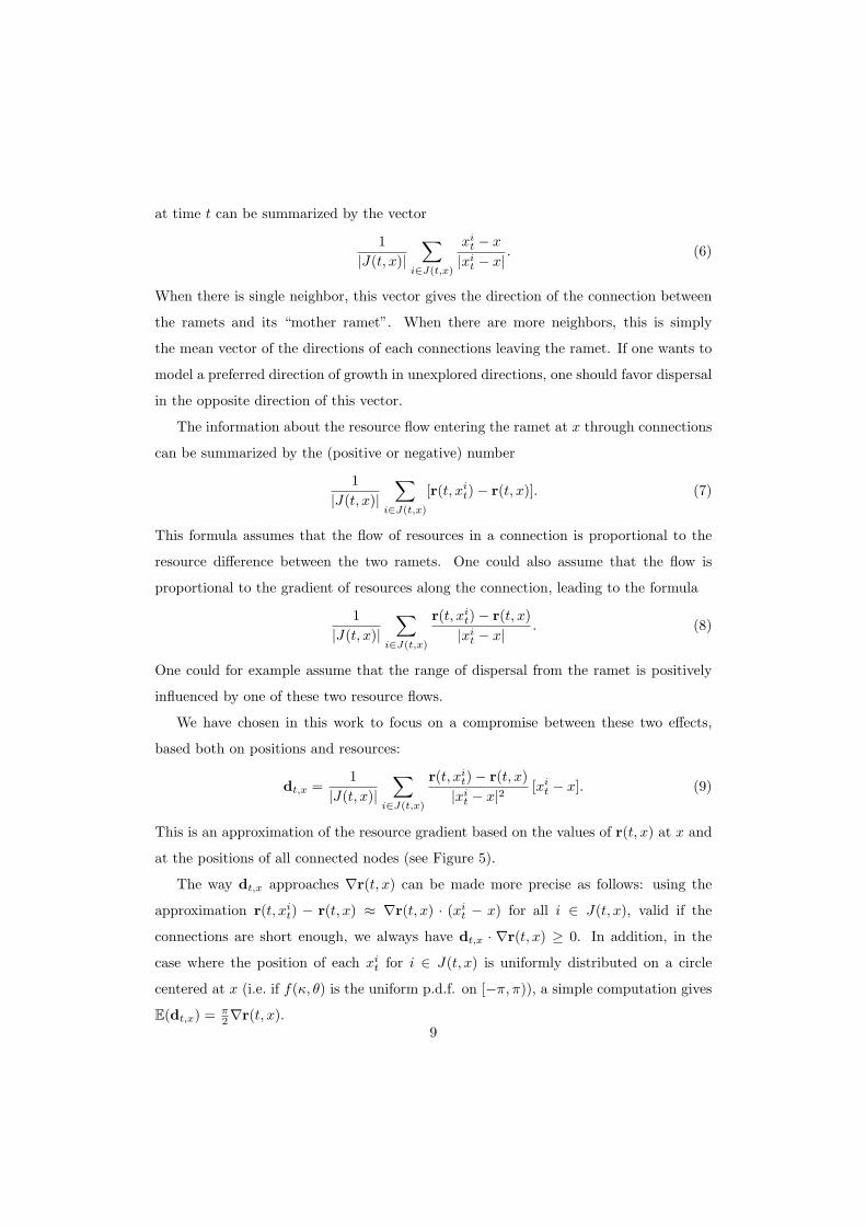
We have chosen in this work to focus on a compromise between these two effects,
based both on positions and resources:
dt,x =1
|J(t, x)|∑
i∈J(t,x)
r(t, xit)− r(t, x)|xit − x|2
[xit − x]. (9)
This is an approximation of the resource gradient based on the values of r(t, x) at x and
at the positions of all connected nodes (see Figure 5).
The way dt,x approaches ∇r(t, x) can be made more precise as follows: using the
approximation r(t, xit) − r(t, x) ≈ ∇r(t, x) · (xit − x) for all i ∈ J(t, x), valid if the
connections are short enough, we always have dt,x · ∇r(t, x) ≥ 0. In addition, in the
case where the position of each xit for i ∈ J(t, x) is uniformly distributed on a circle
centered at x (i.e. if f(κ, θ) is the uniform p.d.f. on [−π, π)), a simple computation gives
E(dt,x) = π2∇r(t, x).
9

4 4.2 4.4 4.6 4.8 5 5.2 5.4 5.6 5.8 60.5
1
1.5
2
2.5
x
x+v
Figure 5: A node in position x will give birth to a new node in position x + v in an approximation of
the gradient of the resources, see (9).
In order to keep the population inside the domain D we simply ignore the new node
y = x+ v when y 6∈ D.
Interactions between nodes and resources
The natural way to model resource concentration is as a density function r(t, x) over
the domain D. Coupling (discrete) individual dynamics with resource density dynamics
is a non-standard problem which requires a choice. We propose the following model:
∂t r(t, x) = div(a(x)∇r(t, x)
)+ b(x) · ∇r(t, x)− r(t, x)α
Nt∑i=1
Γxit(x) (10a)
with r(0, x) = r0(x) and
Γy(x) = exp(− 1
2σ2r|x− y|2) . (10b)
In the absence of plants, the resource concentration r(t, x) follows a classical advec-
tion/diffusion transport equation. The last term of (10a) represents the resource con-
sumption of the ramets. We assume a rate of resource intake proportional to the local
resource concentration during the whole lifetime of each ramet. In addition, we model
with the function Γ the fact that resource consumption is not local. The parameter σr
can then be interpreted as the mean range of roots of a ramet in the species.
The PDE (10) has to be coupled with appropriate boundary conditions. We assume
here that the boundary of the domain D is a natural boundary that cannot be crossed
10

by the plants, because of the absence of resources. This corresponds to the Dirichlet
boundary condition
r(t, x) = 0, ∀x ∈ ∂D .
Of course, other resource consumption models can be considered. For example, consump-
tion can be assumed to occur also at birth, leading to the following resource update at a
birth of a ramet at position y and time t:
r(t, x) = r(t−, x)(1− α′ Γy(x)
).
One could also take into account the degradation of plants at position y after its death
at time t by updating the resource concentration according to
r(t, x) = r(t−, x)(1 + α′′ Γy(x)
),
which corresponds to an instantaneous degradation of the plant.
3. Numerical approximation of the IBM
We now describe the simulation algorithm: starting from the state
νTk−1 =NTk−1∑i=1
δxiTk−1
at last event time Tk−1, we first sample the time of the next event (birth or death):
Tk = Tk−1 + S with S ∼ Exp(λTk−1 + µTk−1
)(11)
and λTk−1 and µTk−1 defined by (3a). The next event:
• is a birth event with probability
λTk−1/(λTk−1 + µTk−1) .
Then sample ı according to
{λ(Tk−1, xiTk−1
)/λTk−1 ; i = 1, . . . , NTk−1}
and v according to the p.d.f. DTk−1,xıTk−1
(v), finally let:
νTk = νTk−1 + δ(xıTk−1
+v)
and update the sets of connections J(Tk, x) accordingly;11
• is a death event with probability
µTk−1/(λTk−1 + µTk−1) .
Then sample ı according to
{µ(Tk−1, xiTk−1
)/µTk−1 ; i = 1, . . . , NTk−1},
let:
νTk = νTk−1 − δxıTk−1
and update the sets of connections J(Tk, x) accordingly.
Note that this algorithm is valid if the rates λ(t, xit) and µ(t, xit) are approximately
constant for t ∈ [Tk−1, Tk−1 + S). If it is not the case, we should make use of an
acceptance/rejection algorithm (Fournier and Meleard, 2004; Campillo and Joannides,
2009). In parallel, we should numerically integrate the PDE (10), for example with
implicit or explicit finite-difference schemes. In practice, if Tk − Tk−1 is small enough,
which is usually the case if the population is large, a single time step of the finite-
difference scheme is sufficient. Note also that, in order to compute the birth and death
rates λ and µ, one needs to interpolate the resource concentration at each ramet position
from the resource concentrations on the discretization grid. The algorithm is presented
in Algorithm 1.
Because the model contains no grid structure, this algorithm is particularly simple to
implement. The state of the process can be coded as a list of each individual’s location
and the labels of its neighbors.
Note also that this algorithm can be very costly when the population size is large, as
it requires us to compute the sums λ and µ at each time step. Another possibility is to
use an acceptance/rejection procedure (Fournier and Meleard, 2004) in order to replace
this sum by a random sampling of the individual to which the next event will apply.
The drawback is that some (and sometimes many) of these events may actually be void,
leading to an increase of the number of time steps in the simulation. In practice, there
is a significant gain of numerical cost for very large populations.
12

T0 ← 0, ν0, r(0, x) givenfor k = 0, 1, . . . do
compute the rates λ(Tk, x), µ(Tk, x), for x ∈ νTkλ←∑
x∈νTk λ(Tk, x), µ←∑x∈νTk µ(Tk, x)
Tk+1 ← Tk + S with S ∼ Exp(λ+ µ)if rand() < λ/(λ+ µ) then
sample x according to {λ(Tk, x)/λ;x ∈ νTk}sample v according to DTk,x(v)νTk+1 ← νTk + δx+v [birth]
elsesample x according to {µ(Tk, x)/µ;x ∈ νTk}νTk+1 ← νTk − δx [death]
end ifcompute r(Tk+1, x) [numerical approximation of (10)]
end for
Algorithm 1: Gillespie algorithm. Here we use the notation x ∈ νt instead of xi fori = 1 · · ·Nt.
4. Simulation
We simulated through this model the growth of two contrasted growth forms: guerril-
las and phalanx growth strategies (sensu Lovett-Doust, 1981) in a heterogeneous resource
concentration landscape. We implemented both types by suitably adjusting the param-
eters of the dispersion kernel in (5):
(i) if the p.d.f. f(κ, θ) of the shoot angle has a large concentration parameter and if the
p.d.f. g(‖v‖) favors large lengths, then the model will present the characteristics of
a guerrilla plant;
(ii) if the p.d.f. f(κ, θ) of the shoot angle has a small concentration parameter and if the
p.d.f. g(‖v‖) favors small lengths, then the model will present the characteristics
of a phalanx plant;
see Figure 6. Examples of resulting plant networks are presented in Figure 7 for the case
of a maximum number of Nmax = 3 connexions per node.
These preliminary simulation tests are run for very simple dynamics of resources: we
assume that there is no advection of resources over the land (b(x) = 0) and that the
diffusion coefficient of resources is constant (a(x) = σ2) in (10a). Since the colonization13
Gue
rrill
a
−3 −2 −1 0 1 2 3
0.5
1
1.5
2
2.5
3
3.5
link angle pdf
f(κ, θ)
0 0.01 0.02 0.03 0.04 0.05
−0.02
−0.01
0
0.01
0.02
0.03
shoot profile
shoots froma given node
2.5 3 3.5 4 4.5 5 5.5 66
6.5
7
7.5
8
8.5
9
9.5
plant dynamics
Pha
lanx
−3 −2 −1 0 1 2 30.1592
0.1592
0.1592
0.1592
0.1592
0.1592
0.1592
link angle pdf
f(κ, θ)
−0.05 −0.04 −0.03 −0.02 −0.01 0 0.01 0.02 0.03 0.04 0.05−0.05
−0.04
−0.03
−0.02
−0.01
0
0.01
0.02
0.03
0.04
0.05
shoot profile
shoots froma given node
2.5 3 3.5 4 4.5 5 5.5 66
6.5
7
7.5
8
8.5
9
9.5
plant dynamics
Figure 6: If the shoot angle p.d.f. f(a, θ) has a large variance (resp.small variance) and if the p.d.f. g(�v�) favors small lengths (resp.large lengths), then the model will present the characteristics of aphalanx growth strategy (resp. guerrilla growth strategy).
for the first point (because the plant grows along straightlines), but inefficient for the second point. Pure Phalanxstrategies are less efficient for the first point, but more effi-cient for the second point (as they grow in all directions).We explore a range of intermediate strategies simply byvarying the variance of the shoot angle distribution f . Asmall variance means that the plant grows nearly alongstraight lines and has a very small probability to changeits growth direction. A large variance corresponds to thecase where the graph structure has no influence on thepopulation dynamics, i.e. the case where f is the uniformdistribution on [0, 2π).
As expected, the simulations of Figure 8 show thatthere is an optimal tradeoff: when the shoot angle p.d.f.is not directive enough or too directive, the plant failsto reach areas with high level of resources; in intermedi-ate cases, the plant reaches these areas and reaches themrapidly.
4.4 4.5 4.6 4.7 4.8 4.9 57
7.1
7.2
7.3
7.4
7.5
7.6
3.8 3.82 3.84 3.86 3.88 3.9 3.92 3.94 3.96 3.98 47.5
7.52
7.54
7.56
7.58
7.6
7.62
7.64
7.66
7.68
7.7
guerilla phalanx
Figure 7: Typical graph patterns for the guerrilla and the phalanxcases. In Figure 9 we present an example where the number ofconnexions per node is limited.
5. Large population approximation of the IBM
Individual-based models are a convenient tool for mod-eling small-scale ecological systems. However, their simu-lation is often costly and can hardly provide relevant field-scale informations in reasonable computational time. Thisis typically the case for phalanx-type clonal plants, wherethe connection length is often short and the plant architec-ture is dense. In order to understand the global interactionbetween plants and resources, the search for simpler ap-proximation models is crucial.
One then typically seeks for partial differential equa-tions (PDE) governing the time dynamics of the popula-tion density over space, obtained in a limit of large pop-ulation. This has been done under various scalings of theindividual parameters for plants systems without networkstructure (Fournier and Meleard, 2004; Champagnat et al.,2006, 2008). Three main families of scalings were describedin the second paper: in the first scaling, space is unscaled,leading to a non-local integro-differential equation for thepopulation density; in the second one, space is scaled, andbirths and deaths are accelerated accordingly in order toobtain a limit, which takes the form of a local reaction-diffusion PDE; in the last scaling, births and deaths areeven more accelerated, leading to a stochastic reaction-diffusion PDE.
Because of the underlying network structure and theexplicit coupling with resource dynamics, these results donot apply directly to our IBM. Similar results can be ob-tained in network-structured populations (Campillo andChampagnat, 2010), but without explicit dynamics for theresources. The result we present here is a first attempt tofill this gap. A full mathematical proof is likely to be verytechnical because our model couples a stochastic, discretestructure for the population and a deterministic, contin-uous structure for resource concentrations. We leave thisproof as an open problem and only present and justifyour macroscopic model as a reasonable large populationapproximation of the IBM.
6
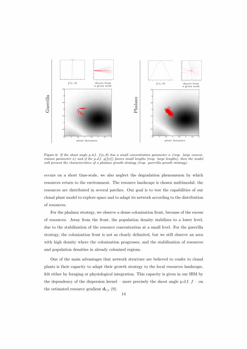
Figure 6: If the shoot angle p.d.f. f(κ, θ) has a small concentration parameter κ (resp. large concen-tration parameter κ) and if the p.d.f. g(‖v‖) favors small lengths (resp. large lengths), then the modelwill present the characteristics of a phalanx growth strategy (resp. guerrilla growth strategy).
occurs on a short time-scale, we also neglect the degradation phenomenon by which
resources return to the environment. The resource landscape is chosen multimodal: the
resources are distributed in several patches. Our goal is to test the capabilities of our
clonal plant model to explore space and to adapt its network according to the distribution
of resources.
For the phalanx strategy, we observe a dense colonization front, because of the excess
of resources. Away from the front, the population density stabilizes to a lower level,
due to the stabilization of the resource concentration at a small level. For the guerrilla
strategy, the colonization front is not as clearly delimited, but we still observe an area
with high density where the colonization progresses, and the stabilization of resources
and population densities in already colonized regions.
One of the main advantages that network structure are believed to confer to clonal
plants is their capacity to adapt their growth strategy to the local resources landscape,
felt either by foraging or physiological integration. This capacity is given in our IBM by
the dependency of the dispersion kernel – more precisely the shoot angle p.d.f. f – on
the estimated resource gradient dt,x (9).14
−3 −2 −1 0 1 2 3−0.8
−0.6
−0.4
−0.2
0
0.2
0.4
0.6
0.8
1
link angle pdf
0 0.2 0.4 0.6 0.8 1 1.2 1.4 1.6 1.8 20
5000
10000
15000
popu
latio
n si
ze
0
10
20
30
40
50
60
70
80
90
reso
urce
evo
lutio
n
−3 −2 −1 0 1 2 3
0.145
0.15
0.155
0.16
0.165
0.17
0.175link angle pdf
0 0.2 0.4 0.6 0.8 1 1.2 1.4 1.6 1.8 20
5000
10000
15000
popu
latio
n si
ze
0
10
20
30
40
50
60
70
80
90
reso
urce
evo
lutio
n
−3 −2 −1 0 1 2 3
0.1
0.12
0.14
0.16
0.18
0.2
0.22
0.24
link angle pdf
0 0.2 0.4 0.6 0.8 1 1.2 1.4 1.6 1.8 20
5000
10000
15000
popu
latio
n si
ze
0
10
20
30
40
50
60
70
80
90
reso
urce
evo
lutio
n
−3 −2 −1 0 1 2 3
0.05
0.1
0.15
0.2
0.25
0.3
0.35
0.4
0.45
0.5
link angle pdf
0 0.2 0.4 0.6 0.8 1 1.2 1.4 1.6 1.8 20
5000
10000
15000
popu
latio
n si
ze
0
10
20
30
40
50
60
70
80
90
reso
urce
evo
lutio
n
−3 −2 −1 0 1 2 3
0.1
0.2
0.3
0.4
0.5
0.6
link angle pdf
0 0.2 0.4 0.6 0.8 1 1.2 1.4 1.6 1.8 20
5000
10000
15000
popu
latio
n si
ze
0
10
20
30
40
50
60
70
80
90
reso
urce
evo
lutio
n
shoot angle p.d.f. f(θ) evolution of the population size (red)
and of the amount of resources (blue)
Figure 8: We assume that for all a > 0, f(a, θ) = f(θ) is the VonMises distribution with variance parameter κ. Taking different val-ues for this parameter (κ = 0, 0.1, 0.5, 2, 3) we plot, on the left,the corresponding shoot angle p.d.f. f(θ) and, on the right, the timeevolution of the size of the population (red) and of the total resource(blue); we suppose that there is no advection of resources (i.e. b ≡ 0in (9)). The simulation is done with the initial resource map ofFigure 3 with high resources spot on the north of the domain, a lessimportant spot in the south and 3 negligible spots (left, center andright), the initial plant is located on the left spot. In the first case,κ = 0, the plant explore all directions without any preference (uni-form distribution of the shoot angle): by chance the plant reachesthe north spot corresponding to the increase of population and thepopulation subsequently decreases. In the second case, κ = 0.1, theplant first reaches the south spot and then the north spot. In thethird case, κ = 0.5, the plant rapidly reaches the north spot andthen the south spot. In the fourth case, κ = 2, the plant need moretime to reach the two important spots. In the last case, the plantdoes not reach any resource spot and node population goes extinctrapidly.
5 5.5 6 6.5 7 7.5 83
3.5
4
4.5
5
5.5
6
4 4.5 5 5.5 6 6.5 72
2.5
3
3.5
4
4.5
5
Guerrilla Phalanx
n
Figure 9: Here the birth rate is adjusted so that each node can havea maximum of 3 connections (i.e. Nmax = 3 in (5)).
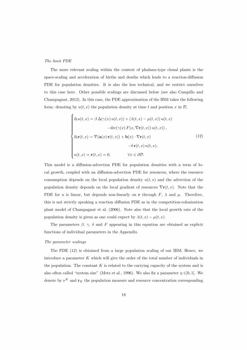
The limit PDEThe more relevant scaling within the context of phalanx-
type clonal plants is the space-scaling and acceleration ofbirths and deaths which leads to a reaction-diffusion PDEfor population densities. It is also the less technical, andwe restrict ourselves to this case here. Concerning otherpossible scalings, we refer to the discussion below (see alsoCampillo and Champagnat. 2010). In this case, the PDEapproximation of the IBM takes the following form: denot-ing by u(t, x) the population density at time t and positionx in D,
∂tu(t, x) = β ∆(γ(x) u(t, x)) + (λ(t, x)− µ(t, x)) u(t, x)−div(γ(x) F (x,∇r(t, x)) u(t, x)) ,
∂tr(t, x) = ∇(a(x) r(t, x)) + b(x) ·∇r(t, x)−δ r(t, x) u(t, x),
u(t, x) = r(t, x) = 0, ∀x ∈ ∂D.
(11)This model is a diffusion-advection PDE with a term oflocal growth for the population density coupled with andiffusion-advection PDE for resources, where the resourceconsumption depends on the local population density u(t, x)and the advection of the population density depends on thelocal gradient of resources ∇r(t, x). Note that the PDE foru is linear, but depends non-linearly on r through F , λ andµ. Therefore, this is not strictly speaking a reaction diffu-sion PDE as in the competition-colonization plant modelof Champagnat et al. (2006). Note also that the localgrowth rate of the population density is given as one couldexpect by λ(t, x)− µ(t, x).
The parameters β, γ, δ and F appearing in this equa-tion are obtained as explicit functions of individual param-eters. Before giving their expression, we first explain thescaling corresponding to this PDE and how it is obtained.
The parameter scalingsFix a parameter η ∈]0, 1[ and introduce a constant K
which will correspond to the order of the population size.This constant K is related to the carrying capacity of thesystem and is also often called “system size” (Metz et al.,
7
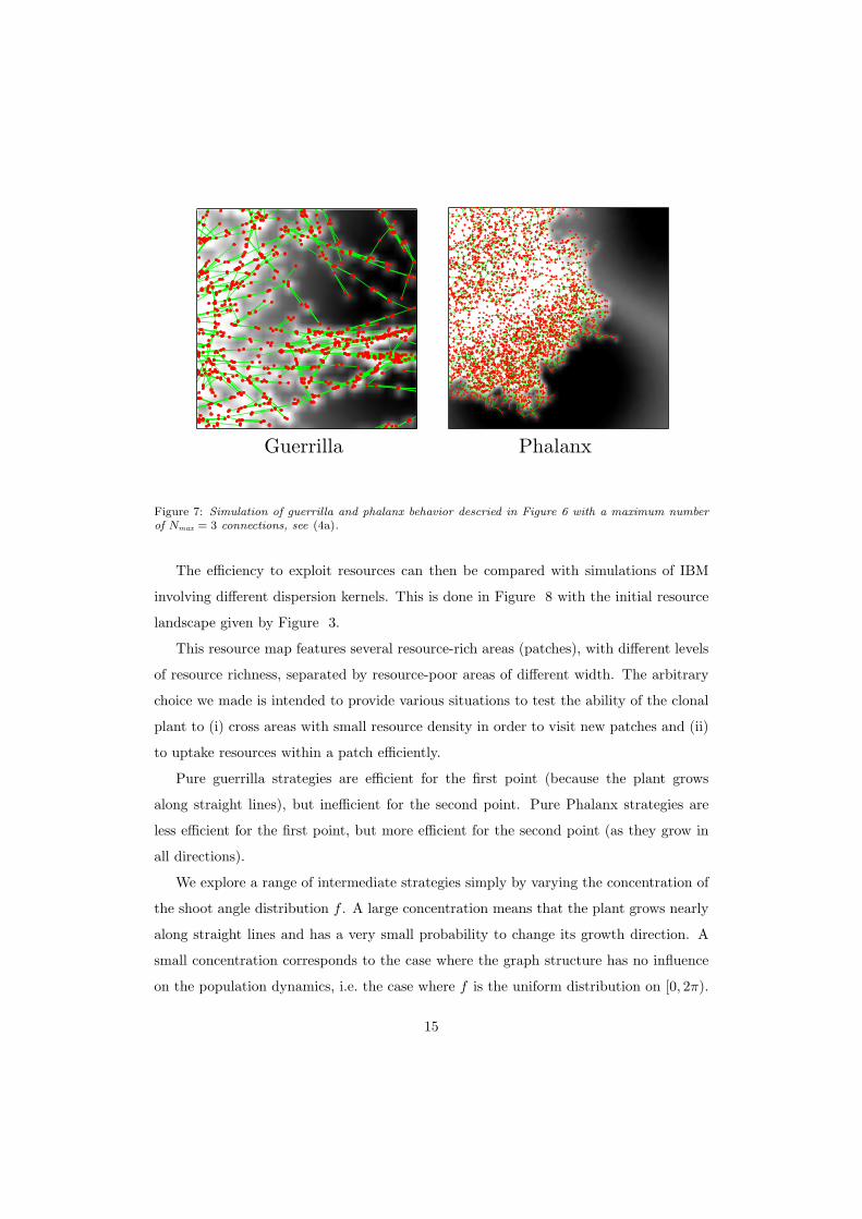
Figure 7: Simulation of guerrilla and phalanx behavior descried in Figure 6 with a maximum numberof Nmax = 3 connections, see (4a).
The efficiency to exploit resources can then be compared with simulations of IBM
involving different dispersion kernels. This is done in Figure 8 with the initial resource
landscape given by Figure 3.
This resource map features several resource-rich areas (patches), with different levels
of resource richness, separated by resource-poor areas of different width. The arbitrary
choice we made is intended to provide various situations to test the ability of the clonal
plant to (i) cross areas with small resource density in order to visit new patches and (ii)
to uptake resources within a patch efficiently.
Pure guerrilla strategies are efficient for the first point (because the plant grows
along straight lines), but inefficient for the second point. Pure Phalanx strategies are
less efficient for the first point, but more efficient for the second point (as they grow in
all directions).
We explore a range of intermediate strategies simply by varying the concentration of
the shoot angle distribution f . A large concentration means that the plant grows nearly
along straight lines and has a very small probability to change its growth direction. A
small concentration corresponds to the case where the graph structure has no influence
on the population dynamics, i.e. the case where f is the uniform distribution on [0, 2π).
15

As expected, the simulations of Figure 8 show that there is an optimal tradeoff: when
the shoot angle p.d.f. is not directive enough or too directive, the plant fails to reach
areas with high level of resources; in intermediate cases, the plant reaches these areas
and reaches them rapidly.
5. Large population approximation of the IBM
Individual-based models are a convenient tool for modelling small-scale ecological sys-
tems. However, their simulation is often costly and can hardly provide relevant field-scale
information in reasonable computational time. This is typically the case for phalanx-type
clonal plants, where the connection length is often short and the plant architecture is
dense. In order to understand the global interaction between plants and resources and to
speed up the computational time, the search for simpler approximation models is crucial.
It is natural to seek partial differential equations (PDE) (El Hamidi et al., 2012)
governing the time dynamics of the population density over space, obtained in a limit of
large population. This has been done under various scalings of the individual parameters
for plants systems without network structure (Fournier and Meleard, 2004; Champagnat
et al., 2006, 2008). Three main families of scalings were described in the second paper:
in the first scaling, space is unscaled, leading to a non-local integro- differential equation
for the population density; in the second one, space is scaled, and births and deaths are
accelerated accordingly in order to obtain a PDE with local reaction-diffusion; in the last
scaling, births and deaths are even more accelerated, leading to a stochastic reaction-
diffusion PDE.
Because of the underlying network structure and the explicit coupling with resource
dynamics, these results do not apply to our IBM. The result we present here is a first
attempt to fill this gap. This is a convergence theorem under appropriate parameter
scalings, so we insist on the fact that the limit is exact. We give in the Appendix an
argument justifying this convergence, but we do not provide a full proof, which would be
very technical because our model couples a stochastic, discrete structure for the popula-
tion and a deterministic, continuous structure for resource concentrations (see Campillo
and Champagnat, 2012, for a proof in a graph-structured IBM without resources).
16

−3 −2 −1 0 1 2 3−0.8
−0.6
−0.4
−0.2
0
0.2
0.4
0.6
0.8
1
link angle pdf
0 0.2 0.4 0.6 0.8 1 1.2 1.4 1.6 1.8 20
5000
10000
15000
popu
latio
n si
ze
0
10
20
30
40
50
60
70
80
90
reso
urce
evo
lutio
n
−3 −2 −1 0 1 2 3
0.145
0.15
0.155
0.16
0.165
0.17
0.175link angle pdf
0 0.2 0.4 0.6 0.8 1 1.2 1.4 1.6 1.8 20
5000
10000
15000
popu
latio
n si
ze
0
10
20
30
40
50
60
70
80
90
reso
urce
evo
lutio
n
−3 −2 −1 0 1 2 3
0.1
0.12
0.14
0.16
0.18
0.2
0.22
0.24
link angle pdf
0 0.2 0.4 0.6 0.8 1 1.2 1.4 1.6 1.8 20
5000
10000
15000
popu
latio
n si
ze
0
10
20
30
40
50
60
70
80
90
reso
urce
evo
lutio
n
−3 −2 −1 0 1 2 3
0.05
0.1
0.15
0.2
0.25
0.3
0.35
0.4
0.45
0.5
link angle pdf
0 0.2 0.4 0.6 0.8 1 1.2 1.4 1.6 1.8 20
5000
10000
15000
popu
latio
n si
ze
0
10
20
30
40
50
60
70
80
90re
sour
ce e
volu
tion
−3 −2 −1 0 1 2 3
0.1
0.2
0.3
0.4
0.5
0.6
link angle pdf
0 0.2 0.4 0.6 0.8 1 1.2 1.4 1.6 1.8 20
5000
10000
15000
popu
latio
n si
ze
0
10
20
30
40
50
60
70
80
90
reso
urce
evo
lutio
n
shoot angle p.d.f. f(θ) evolution of the population size (red)
and of the amount of resources (blue)
Figure 8: We assume that for all a > 0, f(a, θ) = f(θ) is the VonMises distribution with variance parameter κ. Taking different val-ues for this parameter (κ = 0, 0.1, 0.5, 2, 3) we plot, on the left,the corresponding shoot angle p.d.f. f(θ) and, on the right, the timeevolution of the size of the population (red) and of the total resource(blue); we suppose that there is no advection of resources (i.e. b ≡ 0in (9)). The simulation is done with the initial resource map ofFigure 3 with high resources spot on the north of the domain, a lessimportant spot in the south and 3 negligible spots (left, center andright), the initial plant is located on the left spot. In the first case,κ = 0, the plant explore all directions without any preference (uni-form distribution of the shoot angle): by chance the plant reachesthe north spot corresponding to the increase of population and thepopulation subsequently decreases. In the second case, κ = 0.1, theplant first reaches the south spot and then the north spot. In thethird case, κ = 0.5, the plant rapidly reaches the north spot andthen the south spot. In the fourth case, κ = 2, the plant need moretime to reach the two important spots. In the last case, the plantdoes not reach any resource spot and node population goes extinctrapidly.
5 5.5 6 6.5 7 7.5 83
3.5
4
4.5
5
5.5
6
4 4.5 5 5.5 6 6.5 72
2.5
3
3.5
4
4.5
5
Guerrilla Phalanx
n
Figure 9: Here the birth rate is adjusted so that each node can havea maximum of 3 connections (i.e. Nmax = 3 in (5)).
The limit PDEThe more relevant scaling within the context of phalanx-
type clonal plants is the space-scaling and acceleration ofbirths and deaths which leads to a reaction-diffusion PDEfor population densities. It is also the less technical, andwe restrict ourselves to this case here. Concerning otherpossible scalings, we refer to the discussion below (see alsoCampillo and Champagnat. 2010). In this case, the PDEapproximation of the IBM takes the following form: denot-ing by u(t, x) the population density at time t and positionx in D,
∂tu(t, x) = β ∆(γ(x) u(t, x)) + (λ(t, x)− µ(t, x)) u(t, x)−div(γ(x) F (x,∇r(t, x)) u(t, x)) ,
∂tr(t, x) = ∇(a(x) r(t, x)) + b(x) ·∇r(t, x)−δ r(t, x) u(t, x),
u(t, x) = r(t, x) = 0, ∀x ∈ ∂D.
(11)This model is a diffusion-advection PDE with a term oflocal growth for the population density coupled with andiffusion-advection PDE for resources, where the resourceconsumption depends on the local population density u(t, x)and the advection of the population density depends on thelocal gradient of resources ∇r(t, x). Note that the PDE foru is linear, but depends non-linearly on r through F , λ andµ. Therefore, this is not strictly speaking a reaction diffu-sion PDE as in the competition-colonization plant modelof Champagnat et al. (2006). Note also that the localgrowth rate of the population density is given as one couldexpect by λ(t, x)− µ(t, x).
The parameters β, γ, δ and F appearing in this equa-tion are obtained as explicit functions of individual param-eters. Before giving their expression, we first explain thescaling corresponding to this PDE and how it is obtained.
The parameter scalingsFix a parameter η ∈]0, 1[ and introduce a constant K
which will correspond to the order of the population size.This constant K is related to the carrying capacity of thesystem and is also often called “system size” (Metz et al.,
7
Figure 8: Let κ be the concentration parameter of the Von Mises distribution f . Taking different valuesfor this parameter (κ = 0, 0.1, 0.5, 2, 3) we plot, on the left, the corresponding shoot angle p.d.f. f(κ, θ)and, on the right, the time evolution of the size of the population (red) and of the total resource (blue);we suppose that there is no advection of resources (i.e. b ≡ 0 in (10)). The simulation is done with theinitial resource map of Figure 3 with high resources spot on the north of the domain, a less importantspot in the south and 3 negligible spots (left, center and right), the initial plant is located on the left spot.In the first case, κ = 0, the plant explore all directions without any preference (uniform distribution ofthe shoot angle): by chance the plant reaches the north spot corresponding to the increase of populationand the population subsequently decreases. In the second case, κ = 0.1, the plant first reaches the southspot and then the north spot. In the third case, κ = 0.5, the plant rapidly reaches the north spot andthen the south spot. In the fourth case, κ = 2, the plant needs more time to reach the two importantspots. In the last case, the plant does not reach any resource spot and node population goes extinctrapidly.
17
The limit PDE
The more relevant scaling within the context of phalanx-type clonal plants is the
space-scaling and acceleration of births and deaths which leads to a reaction-diffusion
PDE for population densities. It is also the less technical, and we restrict ourselves
to this case here. Other possible scalings are discussed below (see also Campillo and
Champagnat, 2012). In this case, the PDE approximation of the IBM takes the following
form: denoting by u(t, x) the population density at time t and position x in D,
∂tu(t, x) = β∆(γ(x)u(t, x)) + (λ(t, x)− µ(t, x))u(t, x)
−div(γ(x)F (x,∇r(t, x))u(t, x)) ,
∂tr(t, x) = ∇(a(x) r(t, x)) + b(x) · ∇r(t, x)
−δ r(t, x)u(t, x),
u(t, x) = r(t, x) = 0, ∀x ∈ ∂D.
(12)
This model is a diffusion-advection PDE for population densities with a term of lo-
cal growth, coupled with an diffusion-advection PDE for resources, where the resource
consumption depends on the local population density u(t, x) and the advection of the
population density depends on the local gradient of resources ∇r(t, x). Note that the
PDE for u is linear, but depends non-linearly on r through F , λ and µ. Therefore,
this is not strictly speaking a reaction diffusion PDE as in the competition-colonization
plant model of Champagnat et al. (2006). Note also that the local growth rate of the
population density is given as one could expect by λ(t, x)− µ(t, x).
The parameters β, γ, δ and F appearing in this equation are obtained as explicit
functions of individual parameters in the Appendix.
The parameter scalings
The PDE (12) is obtained from a large population scaling of our IBM. Hence, we
introduce a parameter K which will give the order of the total number of individuals in
the population. The constant K is related to the carrying capacity of the system and is
also often called “system size” (Metz et al., 1996). We also fix a parameter η ∈]0, 1[. We
denote by νK and rK the population measure and resource concentration corresponding
18
to the parameter K, and we scale νK as
νKt =1K
NKt∑i=1
δxit .
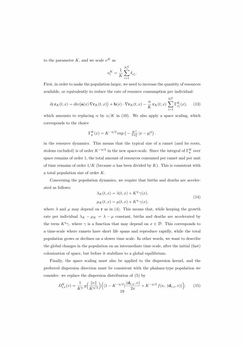
First, in order to make the population larger, we need to increase the quantity of resources
available, or equivalently to reduce the rate of resource consumption per individual:
∂t rK(t, x) = div(a(x)∇rK(t, x)
)+ b(x) · ∇rK(t, x)− α
KrK(t, x)
NKt∑i=1
ΓKxit(x), (13)
which amounts to replacing α by α/K in (10). We also apply a space scaling, which
corresponds to the choice
ΓKy (x) = K−η/2 exp(− Kη
2σ2r|x− y|2) .
in the resource dynamics. This means that the typical size of a ramet (and its roots,
stolons excluded) is of order K−η/2 in the new space-scale. Since the integral of ΓKy over
space remains of order 1, the total amount of resources consumed per ramet and per unit
of time remains of order 1/K (because α has been divided by K). This is consistent with
a total population size of order K.
Concerning the population dynamics, we require that births and deaths are acceler-
ated as follows:λK(t, x) = λ(t, x) +Kη γ(x),
µK(t, x) = µ(t, x) +Kη γ(x),(14)
where λ and µ may depend on r as in (4). This means that, while keeping the growth
rate per individual λK − µK = λ − µ constant, births and deaths are accelerated by
the term Kηγ, where γ is a function that may depend on x ∈ D. This corresponds to
a time-scale where ramets have short life spans and reproduce rapidly, while the total
population grows or declines on a slower time scale. In other words, we want to describe
the global changes in the population on an intermediate time scale, after the initial (fast)
colonization of space, but before it stabilizes to a global equilibrium.
Finally, the space scaling must also be applied to the dispersion kernel, and the
preferred dispersion direction must be consistent with the phalanx-type population we
consider: we replace the dispersion distribution of (5) by
DKt,x(v) =
1Kη
g( ‖v‖Kη/2
)((1−K−η/2)
(dt,x, v)2π
+K−η/2 f(κ, (dt,x, v))). (15)
19

The scaling of the p.d.f. g corresponds to the space scaling of K−η/2 which was used
above for the resource consumption kernel ΓK . The scaling of the p.d.f. f amounts to
a uniform dispersion direction with probability 1−K−η/2 and otherwise to a dispersion
direction around the preferred direction according to f . This corresponds to a population
with nearly no preferred direction, hence a phalanx-type population. Still, the small
probability K−η/2 for a dispersal along the preferred direction has an effect at large space-
scales on the global behavior of the population, corresponding to the term F (x,∇r(t, x))
in the limit PDE (12). This shows that even a small asymmetry in the dispersal direction
for each ramet can lead to a non-negligible global effect. Again, this global effect can be
explicitly expressed in terms of the individual parameters (see Appendix).
6. Discussion
The construction of a model in any scientific domain has to meet several contradictory
goals and must often be a compromise. The first goal is of course the faithfulness of its
results compared to the quantitative results of experiments, and as a consequence, the
details and precision that the model should include in all the relevant mechanisms. The
second goal is its practical interest in terms of prediction, description and analysis of the
phenomenon under study. In this respect, we can distinguish several major issues: the
number of parameters of the model, the difficulty of its numerical implementation, the
numerical cost of its simulation and the possibility of its mathematical analysis. The
tendency to build complicated models to describe natural phenomena has to be faced
with the problems of calibration of too many parameters compared with the amount of
data available, the arbitrary choices that must often be made in the details of the model,
and the numerical cost of its simulation, which can make statistical information or large
time behaviors out of reach.
The construction of a useful model requires to restrict to the significant factors in-
volved in the phenomenon. Of course, the notion of significant factors is highly dependent
of the goals of the study. In Ecology, depending on the spatial scale of the study, one may
prefer to use “realistic IBMs” which aims to describe realistic local population structures,
or “simple IBMs” which focus on a specific feature of the ecosystem and can be used
to study its influence on large space scales. For clonal plants, the first class of models
20

has received much more attention than the second one, and this work is an attempt to
construct a simple IBM for clonal plants which can be numerically and mathematically
studied at the scale of a grassland.
A simple IBM allowing to simulate the growth of two clonal plants
In this work, we presented a simple IBM for clonal plants in continuous time and
space, which can be numerically and mathematically studied on large space-scale. To
this aim, we chose a modelling compromise which consists in substantially simplifying
several aspects of the local architecture of the plant, while focusing on a single aspect: the
influence of the graph structure of the plant on its horizontal growth strategy. Our goal
was to model the influence of the network structure of the plant on its ability to colonize
space (Harper, 1981; Hutchings, 1999) through the exchange of resources and information
along connections (Marshall, 1990; Stuefer et al., 2004; Wijesinghe and Hutchings, 1997;
Hutchings, 1999; Charpentier and Stuefer, 1999; Klimes et al., 1997). This was done by
constructing a preferred horizontal growth direction based on the position and resources
of the neighbors of a ramet in the network. This preferred growth direction influences
the position of new ramets. Because of the importance of resources in the horizontal
growth strategy, we also included an explicit resource dynamics in the model taking the
form of an advection-diffusion partial differential equation.
Typical network architectures of clonal plants range from phalanx to guerrilla strate-
gies (Lovett-Doust, 1981). These strategies strongly influence the horizontal growth of
clonal plants, which in turn strongly influences their colonization and space occupation
abilities (Wildova et al., 2007). Based on a partly exact simulation scheme, as the exact
IBM scheme is coupled with an approximate resources dynamics, the numerical study
of our IBM was done in the context of the colonization of a land with an heterogeneous
and fragmented resource landscape. We proposed a possible parameterization of guerrilla
and phalanx strategies in our model, and we studied the efficiency of these strategies on
the speed of colonization and the resource consumption.
We observed a trade-off between exploration and exploitation inducing contrasted
colonization performance of plants. Space colonization depended on the species clonal
dispersal strategy. Guerilla species were the most efficient at exploring space as their
strategies enable them to colonize space and minimize competition within the clone21

(Lovett-Doust, 1981). These differences in the success of these two strategies are consis-
tent with previous studies (Humphrey and Pike, 1997).
The average distance between two connected ramets and the variance of the gap
between the actual and the preferred directions of growth appear to be particularly im-
portant traits for the plant efficiency. In our simple situation, we observed the existence
of an optimal resource consumption, intermediate between pure phalanx and pure guer-
rilla strategies. The importance of architectural trait in plant performances has been
a key question in clonal plant studies, especially studied through modelling approaches
(Winkler and Schmid, 1995; Wildova et al., 2007; Wong et al., 2011). In particular, an-
gles between branches have been shown to be a key element for determining the ability
of a plant to handle the trade-off between intraclonal competition and space coloniza-
tion (Bell, 1979; Kisljuk et al., 1996; Wong et al., 2011). The model of Smith and
Palmer (1976) demonstrated that a hexagonal architecture would maximize the centrifu-
gal spread and area colonized by the clonal fragment, while generating gaps within it.
Weak variation of this angle disfavors ramet superposition (Bell and Tomlinson, 1980).
Comparison with other classes of IBMs
IBMs on a grid are a convenient way to model the spatial constraints on the network
structure of a plant community without giving too much care to the underlying mecha-
nisms. For example, a spatial grid limits the local spatial density of ramets or spacers,
and the complexity of the network structure. This is probably an important reason for
the success of IBMs on grids for clonal plant modelling.
However, IBMs on grids also have some drawbacks: they can produce unrealistic
structures of the plant (particularly for sympodial species), the spatial constraints are
modelled in an arbitrary way, the numerical implementation of the model can be complex
due to the grid structure, and the models can be analyzed only via simulations.
IBMs in continuous space can answer several of the above mentioned drawbacks: the
absence of grid can solve the spatial artifacts of IBMs with grid; the spatial constraints
can be modelled as a direct consequence of the interaction between plants and resources;
the numerical implementation of the model is very simple and its numerical cost is good
(Section 3); finally, provided they are not too complicated, these models are amenable
to exact macroscopic approximations (Section 5).22

However, IBMs in continuous space also have drawbacks, among which: (i) the graph-
structure of the plant can be unrealistic, since a ramet can produce two very close new
ramets or the local ramet density could be very high; (ii) it is harder to include a realistic
interaction between ramets and resources, since resource concentrations are modelled as
continuous variables over continuous space, whereas individuals are discrete. This last
point is a major difficulty, since the structure of the root system, the mechanisms of
resource absorption by roots (including stolons) and the degradation of the plants are
very complex. We proposed a simple solution for this problem, probably unrealistic.
Still, one can hope that differences on the resource consumption mechanisms at the local
scale have a small influence on larger space-scale. This is supported by our mathematical
analysis in the Appendix, where the resource consumption profile of (10b) only influences
the global dynamics of the population through its mass and its standard deviation σr.
To our knowledge, the mechanism of resource consumption which we use is the first
one proposed in the context of a discrete population and a resource landscape over a
continuous space.
Our model belongs to the family of “simple IBMs”: the basic elements of the plants
are ramets and connections between ramets (rhizomes or stolons), and the above ground
and below ground aspects of the plant are not physically modelled. Of course, this
makes the model unrealistic concerning the local architecture of the plant. However,
our simulations show that our model is able to capture global features of the horizontal
growth of plants, such as guerrilla or phalanx growth strategies.
In addition, our model has a much smaller number of parameters than traditional
IBMs for clonal plants (5 parameters for birth and death rates: the minimal and maximal
birth and death rates and the maximum number of neighbors; 4 parameters for the
dispersal kernel). This makes our model much easier to calibrate than models giving
more details to the plant structure. One of the most promising approaches to calibrate
IBMs lies in the approximate Bayesian computation method (Hartig et al., 2010).
Our purpose was to construct a simple IBM that can be mathematically analized.
However, “realistic IBMs” are a key tool for studying local structures in plant commu-
nities, e.g. for development or behavioral studies. We can propose various extensions of
our model for future studies: (i) to account for unsuccessful exploration of space by the
23
stolon, one can add to the model a probability of actual birth of a new ramet, which
could depend on the local resource concentration; (ii) the birth and death rates (4) may
also depend on resource translocation between ramets (Stuefer et al., 2004), for example
through incoming flow like those defined in (7) or (8); (iii) one can consider external sup-
ply of resources, either with flux (Neumann) boundary conditions or source terms for the
resources PDE (10a); (iv) more generally all information on the plant architecture usu-
ally included in realistic IBMs could be easily translated in models on continuous space.
For example, one can attach variables to each ramet, like their size, age or biomass (for
example, resources attached to a ramet sensu Herben and Novoplansky, 2008), and let
the birth and death parameters depend on these variables. Internal or terminal ramets
could also be distinguished (Oborny and Englert, 2012). Spacers can also disconnect
at a given rate (Herben and Novoplansky, 2008), be characterized by an amount of re-
sources or biomass (physiological integration sensu Stuefer et al., 2004), or grow linearly
in continuous time, similarly as in most of the IBMs of clonal plants on grids.
Towards PDE models for various types of clonal plants
We proposed a PDE model which approaches the IBM when the population is large,
the births and deaths are fast and the size of ramets and spacers is small. This particular
scaling is relevant for clonal plants with phalanx strategies on large space-scales.
The derivation of such a result is usually only possible for “simple IBMs”, and much
easier for IBMs in continuous space. For particle systems on grids, similar results exist,
but usually under mixing assumptions (hence their name of hydrodynamic limits), like
fast motion of individuals (Durrett, 1995; Kipnis and Landim, 1999). Unfortunately,
such assumptions are totally irrelevant for IBMs of plant dynamics. The difficulty comes
from the fact that, without mixing assumptions, IBMs on grids remain influenced by the
geometry of the grid on large space scales (a celebrated example in a different context is
the Wulff crystal shape in statistical mechanics, see Cerf, 2006).
In the class of simple IBMs in continuous space, the first macroscopic results were
obtained using moment equations and their approximation by closure methods under
various space scalings (Bolker and Pacala, 1999; Dieckmann et al., 1999, 2000; Brown
and Bolker, 2004; Bolker, 2004). Afterwards, these results were improved with exact
convergence results to PDEs for population densities, using large space-scale and large24
population asymptotic (Fournier and Meleard, 2004; Champagnat et al., 2006; Campillo
and Joannides, 2009; Meleard and Tran, 2009). All these results were obtained in models
without network structure.
Our method, which makes the connection between IBMs with graph structure in
continuous space, and continuous PDE models, is new and shows how the local details
of the model can keep a non-trivial influence at larger space-scales. In addition, it can
be extended to other scalings of our IBM in the fashion of Champagnat et al. (2008) and
Campillo and Champagnat (2012), or to more complex interactions: (i) the birth, death
and dispersion parameters may also depend on the mean position of the neighbors of a
ramet (6) or on the flow of resources (7) or (8) entering a ramet; (ii) one can also scale
the population size without scaling space, by taking η = 0 in Section 5; in the limit,
the population densities solve a non-local PDE (as the network is unscaled), and must
be expressed also as a function of the age and parent position of a randomly sampled
individual (Campillo and Champagnat, 2012); (iii) our scaling can also be applied to
guerrilla-type strategies, for which the preferred growth direction has a strong influence;
in this case, the limit population density solves a pure advection (or transport) PDE, of
very different nature than the reaction-diffusion PDE obtained for phalanx strategies in
Section 5; (iv) one can also handle the case η = 1, where some demographic stochasticity
remains in the limit of large population, in the fashion of the Fleming-Viot process
(Etheridge, 2004; Champagnat et al., 2006).
Conclusion
By voluntary limiting ourselves to a simple individual-based model, we were able to
propose a precise asymptotic analysis that allowed us to approximate, at the scale of
the field, the IBM by a PDE system. This work is the first result that bridges the gap
between IBM and PDE in the context of clonal plant growth.
This scaling is especially valid for clonal plants with phalanx-type growth. Other
scalings can also be considered for guerrilla-type populations. This is an interesting per-
spective in terms of competition models between two species of clonal plants competing
for common resources. Depending on the scale of study or the species, it could be perti-
nent to consider hybrid models, where one species could be modelled in PDE terms and
the other species could be modelled in IBM terms.25

We believe that the dual representation of IBMs, by means of computer simulation
tools and of mathematical formalisms, will greatly expand in the future.
Appendix — Approximation argument for the limit PDE (12)
Equation (12) can be derived from the scaling described in Section 5 as follows:
we assume that the initial population state νK0 converges to some non-trivial measure
u0(x)dx on D, i.e. that the initial population size is of order K and is distributed over
space close to the population density u0(x). Now, assume that K is large and that at
some time t, the population state νKt is close to the density u(t, x), and consider some
test function φ over D. Then, the quantity At =∫Dφ(x) νKt (dx) changes on the time
interval [t, t+ dt] due to the following three effects:
• Each individual close to x ∈ D gives birth to a number λK(t, x) dt of individuals,
and a proportion µK(t, x) dt die. This gives a local change of the population density
(λK(t, x)− µK(t, x))u(t, x) dt, and a change of At given by∫D
φ(x) (λ(t, x)− µ(t, x))u(t, x) dx dt.
This gives the first-order change of At. Higher-order changes (i.e. changes involving
derivatives of φ) must also be taken into account.
• Among all the births from the individuals around x ∈ D, a proportion 1−K−η/2are located symmetrically around x at a distance K−η/2 ρ, where ρ is distributed
as g(ρ). Making a Taylor expansion of φ around x, the corresponding change of At
is given by
dt
∫D
dxλK(t, x)u(t, x)∫ 2π
0
dθ
2π
∫ +∞
0
g(ρ) dρ×
12 (ρK−η/2 vθ)′∇2 φ(x) (ρK−η/2 vθ),
where vθ = (cos θ, sin θ) is the unit vector of direction θ. Note that the first-order
term does not appear as it vanishes because of the symmetry of dispersions. Note
also that the scaling of λK in (14) has been chosen so that it exactly cancels the
scaling of the dispersion distance K−η/2ρ. Neglecting the smaller order terms, an
26

easy computation gives a change of At of∫ +∞0
ρ2 g(ρ) dρ4
∫D
∆φ(x) γ(x)u(t, x) dx dt.
• Among all the births from the individuals around x ∈ D, a proportion K−η/2
are located at x + K−η/2v, where v has distribution (5). Making again a Taylor
expansion of φ, we obtain a local change of At of
dt
∫D
K−η/2λK(t, x)u(t, x)∇φ(x) ·K−η/2〈vt,x〉 dx,
where 〈vt,x〉 is the mean of vt,x when v has distribution (5), in which dt,x has the
distribution of the preferred dispersion direction in the population around x. Of
course, this last distribution is unknown and must be computed (see below).
Putting together all the previous results, we obtain
dAtdt
=∫D
( R +∞0 ρ2 g(ρ) dρ
4 ∆φ(x) γ(x)u(t, x)
+ φ(x) (λ(t, x)− µ(t, x))u(t, x) +∇φ(x) 〈vt,x〉 γ(x)u(t, x))dx .
This is the weak formulation of the PDE (12), where we put
β =
∫ +∞0
ρ2 g(ρ) dρ4
,
F (x,∇r(t, x)) = 〈vt,x〉.
The fact that 〈vt,x〉 only depends on x and ∇r(t, x) will be justified below.
Before coming to the computation of F , we observe that the last term of the PDE (13)
for rK may be written as
−α rK(t, x)∫D
ΓKy (x)νK(dy).
Replacing νK(dy) with its limit u(t, y)dy and passing to the limit K → +∞ would
formally give the second equation of (12) with
δ =α√
2π σr
.
However, this requires a sufficient regularity for u(t, x) and a convergence of νKt (dy) to
u(t, y)dy such that space means of νKt over balls of diameter of the order of K−η/2 also27
converge to u(t, x). This is the place where a full mathematical proof requires a careful
analysis that we do not examine here.
Finally, we need to compute the distribution of the preferred dispersion direction over
the population close to a fixed x ∈ D at a fixed time t ≥ 0. We consider one of these
ramets chosen at random and call it RSI (Randomly Sampled Individual) at x, and we
divide the computation into several steps.
Scaled age distribution of a RSI
Because of the scaling of the death rate µK(t, x), the life span of the RSI is of order
K−η, and the position of its mother ramet is at a distance of order K−η/2 because of
the scaling of the p.d.f. g. Over these time and space scales, the population densities
and resource concentration can be assumed constant equal to u(t, x) and r(t, x). We call
scaled age of an individual at x at time t, its age multiplied by Kη.
In particular, the ramets alive at time t close to x appeared at an (approximately)
constant rate during a time length of order K−η. Since they die (approximately) at
constant rate Kηγ(x), the probability of survival of an individual born at time t− yK−ηis e−yγ(x). Since the birth rate of individuals close to x is approximately constant, we
deduce that the scaled age of a RSI at x is asymptotically distributed when K → +∞as an exponential random variable with parameter γ(x).
Number of living offsprings of a RSI
Conditionally on the age K−ηy (or the scaled age y) of a RSI at x, the birth rate at x
over the time interval [t−K−ηy, t] is (approximately) constant equal to Kηγ(x). There-
fore, the scaled age of all its offspring is distributed as a Poisson process of parameter
γ(x) on the interval [0, y]. In particular, the total number of offsprings is distributed as
a Poisson random variable with parameter yγ(x). Among them, some are already dead
at time t.
In order to compute the number of living neighbors of the RSI, we need to introduce an
additional conditioning on the number k of offspring of a RSI conditioned to have scaled
age y. We use the following feature of Poisson processes: conditionally of the number k
of offspring of the RSI, their scaled age are distributed as k independent and identically
distributed (i.i.d.) random variables with uniform distribution on [0, y]. In other words,28

conditionally on the age K−ηy of the RSI and the number of its children k, the ages
of its children are distributed as k i.i.d. random variable with uniform distribution on
[0,K−ηy].
Since they all die at (approximate) rate Kηγ(x), the survival probability of each is
1K−ηy
∫ K−ηy
0
e−Kηγ(x)sds =
1− e−yγ(x)yγ(x)
.
We denote by px,y the right-hand side of this equation. This leads to a number of living
children of the RSI with binomial distribution with parameters k and px,y.
Number of living neighbors of a RSI
Similarly, conditionally on the scaled age y of the RSI, its mother ramet is still alive
at time t with probability e−yγ(x).
Therefore, the number N of living neighbors of a RSI at x conditionally on A = y,
where A is the scaled age of the RSI, is distributed as
P(N = n | A = y) = e−y γ(x)∑
k≥n−1
e−y γ(x)(y γ(x))k
k!
(k
n− 1
)pn−1x,y (1− px,y)k−n+1
+ (1− e−y γ(x))∑k≥n
e−y γ(x)(y γ(x))k
k!
(k
n
)pnx,y(1− px,y)k−n,
for n ≥ 1 and
P(N = 0 | A = y) = (1− e−y γ(x))∑k≥0
e−y γ(x)(y γ(x))k
k!(1− px,y)k.
Denoting for convenience these quantities qx,y(n), we obtain the following distribution
for the number N of living neighbors of a RSI at x: for all n ≥ 0,
P(N = n) =∫ +∞
0
γ(x)e−y γ(x) qx,y(n) dy. (16)
Positions of the neighbors of a RSI
Neglecting the smaller-order terms in (15), we have
DKt,x ≈ 1
Kη g(‖v‖Kη/2
)(dt,x,v)
2π ,
which means that the direction of dispersal is (approximately) uniform for each birth.
This is also the case for the births from the RSI at x, as well as its mother ramet.
Therefore, the positions of all the neighbors of the RSI at x are i.i.d. and distributed as
x+K−η/2ρvθ, where ρ has p.d.f. g(ρ) and vθ = (cos θ, sin θ).29
Asymptotic distribution of dt,x
Since the length of connections is of order K−η/2, we can replace r(t, xit) − r(t, x)
with ∇r(t, x) · (xit − x) in the formula (9) for the preferred dispersion direction dt,x.
Therefore, conditionally on N = n ≥ 1, the preferred dispersion direction dt,x of a RSI
at x is distributed as1n
n∑i=1
(∇r(t, x) · vθi)vθi , (17)
where θ1, θ2, . . . are i.i.d. random variable uniformly distributed on [0, 2π).
Introducing θt,x such that ∇r(t, x) = ‖∇r(t, x)‖ vθt,x , and applying the rotation of
angle −θt,x to the vector (17) yields
1n
n∑i=1
cos(θ′i) vθ′i , (18)
where the θ′i are i.i.d. and uniformly distributed on [0, 2π).
Denoting by µ(w)dw the distribution of cos(θ)vθ for θ uniformly distributed on [0, 2π),
the distribution of the vector (18) is µ∗n(nw) dw, where µ∗n = µ ∗ . . . ∗ µ and ∗ denotes
the convolution operator. Therefore, a RSI at x at time t has the following distribution
for its preferred dispersal direction dt,x rotated of the angle −θt,x:
P(N = 0) δ0(dw) +∑n≥1
P(N = n)µ∗n(nw) dw
where P(N = n) is given by (16). Denoting by π(dw) the previous distribution, we finally
obtain
F (x,∇r(t, x)) = 〈vt,x〉 =∫
R2π(dw)
∫ 2π
0
dθ
∫ +∞
0
dρ ρ vθt,x+θ f(κ(‖w‖), (w, vθ)
)g(ρ) .
Note that the right-hand side only depends on x through the distribution of N , and on
∇r(t, x) through the angle θt,x.
Acknowledgment: We are very grateful to Cendrine Mony who gave us valuable advices
and comments on a preliminary version of this work.
References
Bell, A.D., 1979. The hexagonal branching pattern of rhizomes of Alpinia speciosa L. (Zingieraceae).Ann. Bot. 43, 209–223.
30

Bell, A. D., Tomlison, P. B., 1980. Adaptive architecture in rhizomatous plants. Bot. J. Linn. Soc. 80,125-160.
Birch, D. A., Young, W. R., 2006. A master equation for a spatial population model with pair interactions.Theoretical Population Biology 70 (1), 26–42.
Bolker B. M., 2004. Continuous-space models for population dynamics. In: I. Hansi and O. E. Gaggioti(Eds.), Ecology, Genetics and Evolution of Metapopulations, pp. 45–69. Elsevier Science, San Diego,CA.
Bolker, B. M., Pacala, S. W., 1999. Spatial moment equations for plant competition: understandingspatial strategies and the advantages of short dispersal. American Naturalist 153, 575–602.
Brown, D. H., Bolker, B. M., 2004. The effects of disease dispersal and host clustering on the epidemicthreshold in plants. Bulletin of Mathematical Biology 66, 341–371.
Campillo, F., Champagnat, N., 2012. Large population scalings for individual-based stochastic modelsof graph-structured populations, in preparation.
Campillo, F., Joannides, M., 2009. A spatially explicit Markovian individual-based model for terrestrialplant dynamics. ArXiv Mathematics e-prints (arXiv:0904.3632v1).
Cerf, R, 2006. The Wulff crystal in Ising and Percolation models. Lecture Notes in Mathematics 1878,Springer-Verlag, Berlin.
Champagnat, N., Ferriere, R., Meleard, S., 2006. Unifying evolutionary dynamics: from individualstochastic processes to macroscopic models. Theoretical Population Biology 69 (3), 297–321.
Champagnat, N., Ferriere, R., Meleard, S., 2008. From individual stochastic processes to macroscopicmodels in adaptive evolution. Stochastic Models 24, Suppl. 1, 2–44.
Champagnat, N., Meleard, S., 2011. Polymorphic evolution sequence and evolutionary branching. Prob-ability Theory and Related Fields 151 (1), 45–94.
Charpentier, A., Stuefer, J. F., 1999. Functional specialization of ramets in Scirpus maritimus. PlantEcology 141, 129–136.
Cheplick, G. P., 1997. Responses to severe competitive stress in a clonal plant: differences betweengenotypes. Oikos 79:581–591.
DeAngelis, D. L., Gross, L. J. (Eds.), 1992. Individual-based models and approaches in ecology: popu-lations, communities and ecosystems. Chapman and Hall.
Dieckmann, U., Herben, T., Law, R., 1999. Spatio-temporal processes in ecological communities. CWIQuarterly 12, 213–238.
Dieckmann, U., Law, R., May 1996. The dynamical theory of coevolution: a derivation from stochasticecological processes. Journal of Mathematical Biology 34 (5), 579–612.
Dieckmann, U., Law, R., Metz, J. A. J. (Eds.), 2000. The Geometry of Ecological Interactions: Simpli-fying Spatial Complexity. Cambridge University Press.
Durrett, R., 1995. Ten lectures on particle systems. In: Lectures on Probability Theory (Saint Flour,1993). Lecture Notes in Mathematics 1608, pp. 97–201. Springer-Verlag, Berlin.
El Hamidi, A., Garbey, M., Ali, N., 2012. On nonlinear coupled diffusions in competition systems.Nonlinear Analysis: Real World Applications 13(3), 1306–1318.
Etheridge, A. M., 2004. Survival and extinction in a locally regulated population. Annals of AppliedProbability 14 (1), 188–214.
Fournier, N., Meleard, S., 2004. A microscopic probabilistic description of a locally regulated populationand macroscopic approximations. Annals of Applied Probability 14, 1880–1919.
Grimm, V., Railsback, S. F., 2005. Individual-based Modeling and Ecology. Princeton University Press.Harper, J. L., 1981. The concept of the modular organism. In R. M. May (ed.), Theoretical ecology:
Principles and applications, 2nd edn. Sinauer, Sunderland: 53–77.Hartig, F., Calabrese, J. M., Reineking, B., Wiegand, T., Huth, A., 2011. Statistical inference for
stochastic simulation models – theory and application. Ecol. Lett. 14(8), 816–827.Herben, T., Novoplansky, A., 2008. Implications of self/non-self discrimination for spatial patterning of
clonal plants. Evol. Ecol. 22, 337–350.Herben, T., Suzuki, J.-I., 2002. A simulation study of the effects of architectural constraints and resource
translocation on population structure and competition in clonal plants. Evolutionary Ecology 15, 403–423.
Humphrey, L.D., Pyke, D.A., 1997. Clonal foraging in perennial wheatgrasses - A strategy for exploitingpatchy soil nutrients. Journal of Ecology, 85 (5), 601–610.
Humphrey, D.L., Pyke, D.A., 1998. Demographic and growth responses of a guerrilla and a phalanxperennial grass in competitive mixtures. Journal of Ecology 86 (5), 854–865.
Hutchings, M. J., 1999. Clonal plants as cooperative systems: benefits in heterogeneous environments.Plant Species Biology 14, 1–10.
31

Kisljuk, O.S., Kusnetzova, T.V., Agafonova, A.A., 1996. On the modeling of clone geometry in Asarumeuropaeum. J. Theor. Biol. 178, 399–404.
Kipnis, C., Landim, C., 1999. Scaling limits of interacting particle systems. Springer-Verlag, Berlin.Klimes, L., Klimesova, J., Hendriks, R. J. J., van Groenendael, J., 1997. Clonal plants architectures: a
comparative analysis of form and function. In: de Kroon, H., van Groenendale, J. (Eds.), The Ecologyand Evolution of Clonal Plants. Backhuys Publishers, Leiden, pp. 1–29.
Kun, A., Oborny, B., 2003. Survival and competition of clonal plant populations in spatially and tem-porally heterogeneous habitats. Community Ecology 4, 1–20.
Lovett-Doust L. 1981. Population dynamics and local specialization in a clonal perennial (Ranunculusrepens). Journal of Ecology 69: 743–755.
Marshall, C., 1990. Source–sink relations of interconnected ramets. In J. van Groenendael and H. deKroon (Eds.) Clonal Growth in Plants: Regulation and Function. SPB Academic Publishing, TheHague, pp. 23–41.
Meleard, S., Tran, V. C., 2009. Trait substitution sequence process and canonical equation for age-structured populations. Journal of Mathematical Biology 58 (6), 881–921.
Metz, J. A. J., Geritz, S. A. H., Meszena, G., Jacobs, F. J. A., van Heerwaarden, J. S., 1996. Adaptivedynamics, a geometrical study of the consequences of nearly faithful reproduction. In: Stochastic andspatial structures of dynamical systems (Amsterdam, 1995). Konink. Nederl. Akad. Wetensch. Verh.Afd. Natuurk. Eerste Reeks, 45. North-Holland, Amsterdam, pp. 183–231.
Mony, C., Garbey, M., Smaoui, M., Benot, M. L., 2012. Large Scale Parameter Study of an IndividualBased Model of Clonal Plant with Volunteer Computing. To appear in Ecological Modelling.
Novoplansky, A., 2009. Picking battles wisely: plant behaviour under competition. Plant Cell Environ.32, 726–741.
Oborny, B., 1994. Growth rules in clonal plants and environmental predictability – a simulation study.Journal of Ecology 82, 341–351.
Oborny, B., Czaran, T., Kun, A., 2001. Exploration and exploitation of resource patches by clonal growth:a spatial model on the effect of transport between modules. Ecological Modelling 141, 151–169.
Oborny, B., Englert, P., 2012. Plant growth and foraging for a patchy resource: A credit model. Toappear in Ecological Modelling.
Oborny, B., Kun, A., 2002. Fragmentation of clones: how does it influence dispersal and competitiveability? Evolutionary Ecology 15, 319–346.
Oborny, B., Kun, A., Czaran, T., Bokros, S., 2000. The effect of clonal integration on plant competitionfor mosaic habitat space. Ecology 81, 3291–3304.
Smith, A. P., Palmer, J. O. 1976, Vegetative reproduction and close packing in a successional plantspecies. Nature 261, 232–23.
Stuefer, J., Gomez, S., Van Molken, T., 2004. Clonal integration beyond resource sharing: implicationsfor defence signalling and desease transmission in clonal plant networks. Evolutionary Ecology 18,647—667.
van Groenendael, J.M., Klimes, L., Klimesova, J., Hendricks, R.J.J., 1996. Comparative ecology of clonalplants. Philos Trans. R. Soc. Lond. B 351, 1331–1339.
van Kleunen, M., Fischer, M., 2001. Adaptive evolution of plastic foraging responses in a clonal plant.Ecology 82(12), 3309–3319
Wijesinghe, D. K., Hutchings, M. J., 1997. The effects of spatial scale of environmental heterogeneity onthe growth of clonal plant: An experimental study with Glechoma hederacea. Journal of Ecology 85,17–28.
Wildova, R., Gough, L., Herben, T., Hershock, C., Goldberg, D., 2007. Architectural and growth traitsdiffer in effects on performance of clonal plants: an analysis using a field-parameterized simulationmodel. Oikos 116, 836–852.
Winkler, E., Fischer, M., 2002. The role of vegetative spread and seed dispersal for optimal life historiesof clonal plants: a simulation study. Evolutionary Ecology 15 (4-6), 1573–8477.
Winkler, E., Fischer, M., Schmid, B., 1999. Modelling the competitiveness of clonal plants by comple-mentary analytical and simulation approaches. Oikos 85, 217–233.
Winkler, E., Klotz, S., 1997. Clonal plant species in a dry-grassland community: A simulation study oflong-term population dynamics. Ecological Modelling 96 (1-3), 125 – 141.
Winkler, E. and Schmid, B., 1995. Clonal strategies of herbaceous plant species - a simulation study onpopulation growth and competition. Abstracta Bot., 19: 17-28.
Winkler, E., Stocklin, J., 2002. Sexual and vegetative reproduction of Hieracium pilosella L. undercompetition and disturbance: a grid-based simulation model. Annals of Botany 89, 525–536.
Wong, S., Anand, M., Bauch, C.T., 2011. Agent-based modelling of clonal plant propagation across
32

space: recapturing fairy rings and other real-world phenomena. Ecological Informatics 6: 127-135.
33