SIMULATION ANALYSES OF CONTINUOUS STIRRED TANK REACTOR

Jiri Vojtesek and Petr Dostal Faculty of Applied Informatics Tomas Bata University in Zlin

Nad Stranemi 4511, 760 05 Zlin, Czech Republic E-mail: {vojtesek,dostalp}@fai.utb.cz

KEYWORDS CSTR, Adaptive control, Polynomial approach, LQ, Recursive identification ABSTRACT

This paper presents simulation experiments on the continuous stirred tank reactor (CSTR) which is widely used equipment mainly in the chemical industry. The behaviour of these types of systems is usually nonlinear with other negative properties such as a time-delay or a non-minimum phase behaviour and simulation could help us with the understanding of them without making real experiments which could be dangerous, time or cost demanding. The simple iteration method and the Runge-Kutta’s method were used for solving of a steady-state and dynamics of the system. Used adaptive control is based on the recursive identification of an External Linear Model (ELM) as a representation of the originally nonlinear system. The polynomial approach together with the LQ approach gives sufficient control results although the system has negative control properties. INTRODUCTION

The simulation of the system on a computer enroll big boom nowadays when speed and availability of the computer technologies grows rapidly. On the contrary, the purchasing prise and running costs are relatively low. The computer simulation is usually connected with the mathematical model as a result of modeling procedure (Ingham et al. 2000). Material and heat balances are one way how to describe the system and relations between unknown quantities in the mathematical way. These balances are then represented by ordinary or partial differential equations depending on the type of systems. The Continuous Stirred Tank Reactor (CSTR) is typical equipment used in the industry for its good properties from control point of view. The CSTR belongs to the class of lumped parameters systems, a mathematical model of which is described by the set of ordinary differential equations (ODE). The simulation analysis of the system usually consists of steady-state and dynamic analyses (Ingham et al. 2000, Luyben 1989). The simple iteration method and Runge-Kutta’s method (Lyuben 1989) were used in the work for numerical solving of the steady-state and

dynamic analyses. These methods are well known, simple and Runge-Kutta’s method is fully implemented in the used mathematical software Matlab. Results from simulation experiments are then used for choosing of the control strategy and designing of the controller. The nonlinearity and negative control properties of the system should be overcome with the use of Adaptive control (Åström 1989). Adaptive approach used in this work is based the choice of an External Linear Model (ELM) parameters of which are recomputed recursively during the control (Bobal et al. 2005). The external delta models (Middleton and Goodwin 2004) were used for parameter estimation. Although delta models belong to the range of discrete models, parameters of these models approaches to their continuous-time counterparts up to some assumptions (Stericker and Sinha 1993). Ordinary recursive least squares method (Fikar and Mikles 1999) was used for parameter estimation during the control. A polynomial approach with one degree-of-freedom (1DOF) configuration used for the controller synthesis has satisfied basic control requirements and connected with the LQ control technique, it fulfills the requirements of stability, asymptotic tracking of the reference signal and compensation of disturbances (Kucera 1993). MODEL OF THE PLANT

As it is written above, the chemical process under consideration is the Continuous Stirred Tank Reactor (CSTR). The schematical representation of the CSTR is in Figure 1. We supposed that reactant is perfectly mixed and react to the final product with the concentration cA(t). The heat produced by the reaction is represented by the temperature of the reactant T(t). Furthermore we expect that volume, heat capacities and densities are constant during the control due to simplification. A mathematical model of this system is derived from the material and heat balances of the reactant and cooling. The resulted model is then set of two Ordinary Differential Equations (ODEs) (Gao et al. 2002):

( ) ( )

( )

4

1 0 2 1 3 0

1 0 1

1 c

aq

A c

AA A A

dT a T T a k c a q e T Tdt

dca c c k c

dt

⎛ ⎞⎜ ⎟= ⋅ − + ⋅ ⋅ + ⋅ ⋅ − ⋅ −⎜ ⎟⎜ ⎟⎝ ⎠

= ⋅ − − ⋅

(1)

Proceedings 22nd European Conference on Modelling andSimulation ©ECMS Loucas S. Louca, Yiorgos Chrysanthou,Zuzana Oplatková, Khalid Al-Begain (Editors)ISBN: 978-0-9553018-5-8 / ISBN: 978-0-9553018-6-5 (CD)

Where a1-4 are constants computed as

1 2 3 4; ; ;c pc a

p p c pc

c hq Ha a a aV c c V c

ρ

ρ ρ ρ

⋅ −−Δ= = = =

⋅ ⋅ ⋅ ⋅ (2)

variable t in previous equations denotes time, T is used for temperature of the reactant, V is volume of the reactor, cA represents concentration of the product, q and qc are volumetric flow rates of the reactant and cooling respectively. Indexes (·)0 denotes inlet values of the variables and (·)c is used for variables related to the cooling. The fixed values of the system are shown in Table 1 (Gao et al. 2002). The reaction rate, k1, is computed from Arrhenius law:

1 0 eE

R Tk k−⋅= ⋅ (3)

where k0 is reaction rate constant, E denotes an activation energy and R is a gas constant. As you can see, this reaction rate is nonlinear function of the temperature T and we can say, that this system is a nonlinear system with lumped parameters.

Figure 1: Continuous Stirred Tank Reactor

Table 1: Fixed parameters of the reactor

Reactant’s flow rate Reactor’s volume Reaction rate constant Activation energy to R Reactant’s feed temperature Reaction heat Specific heat of the reactant Specific heat of the cooling Density of the reactant Density of the cooling Feed concentration Heat transfer coefficient

q = 100 l.min-1 V = 100 l

k0 = 7.2·1010 min-1 E/R = 1·104 K

T0 = 350 K ΔH = -2·105 cal.mol-1

cp = 1 cal.g-1.K-1 cpc = 1 cal.g-1.K-1 ρ = 1·103 g.l-1 ρc = 1·103 g.l-1 cA0 = 1 mol.l-1

ha = 7·105 cal.min-1.K-1

STEADY-STATE AND DYNAMIC ANALYSES

The system is submitted to the steady-state and dynamic analyses to obtain information about the behaviour of the system.

Steady-state Analysis The steady-state analysis shows behaviour of the system in the steady-state, i.e. in t ∞ and results in optimal working point in the sense of maximal effectiveness and concentration yield. Mathematical meaning of the steady-state is that derivatives with respect to time variable are equal to zero, d(·)/dt = 0. The mathematical model (1) is then transferred to the set of two nonlinear equations:

4

4

1 0 2 1 3 0

1 3

1 0

1 1

1

1

c

c

aqs

A c

saq

c

s AA

a T a k c a q T e

T

a a q e

a cc

a k

⎛ ⎞⋅ + ⋅ ⋅ + ⋅ ⋅ ⋅⎜ − ⎟

⎜ ⎟⎝ ⎠=

⎛ ⎞+ ⋅ ⋅⎜ − ⎟

⎜ ⎟⎝ ⎠

⋅=

+

(4)

The simple iteration method was used for solving of this set of equation and the results are shown in figures. The steady-state analysis was done for different volumetric flow rate of the reactant q = <100; 200> in l.min-1 and different volumetric flow rate of the cooling qc = <20; 100> l.min-1.

100120

140160

180200

2040

6080

100

0.95

0.96

0.97

0.98

qc [l.min -1]

cs A [m

ol.l-1

]q [l.m

in-1 ]

Figure 2: Steady-state values of concentration cA for

different volumetric flow rates q and qc

100120

140160

180200

2040

6080

100

352

354

356

358

360

Ts [K]

qc [l.min -1]

q [l.min

-1 ]

Figure 3: Steady-state values of temperature T for

different volumetric flow rates q and qc

As it could be seen in previous figures, system has nonlinear behaviour as we expected from the mathematical model. We cannot choose the exact optimal working point from figures but from the practical and mainly cost point of view is eligible to choose volumetric flow rates as low as possible. The working point is then characterized by the pair of volumetric flow rates: 1 180 . 100 .cq l min q l min− −= = (5) The steady-state values of state variables T and are cA for this working point 1354.26 0.9620 .s s

AT K c mol l−= = (6) Dynamic Analysis This analysis means that we observe course of the state variables in time after the step change of some input variable. The step changes of volumetric flow rates q and qc are input variables in our case and the steady-statel values in Equation (6) are initial conditions for the set of ODE (1). The Runge-Kutta’s fourth order method was used for numerical solving of the set of ODE. Six step changes of each input variable (±80%, ±40%, ±20% of its value in working point (5)) were done and the results are shown in Figure 4 – Figure 7 . The output variables y1 and y2 represents difference between the actual value and the steady-state value of the variable: ( ) ( ) ( ) ( )1 2;s s

A Ay t T t T y t c t c= − = − (7)

0 5 10 15 20 25 30

-1.0

-0.5

0.0

0.5

1.0

1.5

2.0

2.5

3.0

-60%-40%-20%

+20%

+40%

y 1(t) [K

]

t [min]

+60%

Figure 4: Time response of the output y1 for various

step changes of the input volumetric flow rate of cooling Δqc

0 5 10 15 20 25 30

-0.010

-0.008

-0.006

-0.004

-0.002

0.000

0.002

0.004

y 2(t)

[mol

.l-1]

t [min]

-40%-60%

-20%

+20%

+40%

+60%

Figure 5: Time response of the output y2 for various

step changes of the input volumetric flow rate of cooling Δqc

Step responses in Figure 4 and Figure 5 show that the output temperature, y1, could be described by the first or the second order transfer function and the second order transfer function could be used as a description of the output – concentration cA represented by y2.

0 5 10 15 20 25 30

-1

0

1

2

3

4

y 1(t) [K

]

t [min]

-40%-60%

-20%

+20%

+40%

+60%

Figure 6: Time response of the output y1 for various step changes of the input volumetric flow rate of reactant Δq

0 5 10 15 20 25 30

-0.075

-0.050

-0.025

0.000

0.025

y 2(t) [m

ol.l-1

]

t [min]

-40%-60%

-20%

+20%

+40%

+60%

Figure 7: Time response of the output y2 for various

step changes of the input volumetric flow rate of reactant Δq

The second dynamic analysis for different step changes of the reactant’s flow rate results in similar responses as in the previous case – see Figure 6 and Figure 7. ADAPTIVE CONTROL

The input (control) variable is the change of the volumetric flow rate of the coolant and the output (controlled) variable is temperature of the reactant, i.e.

( ) ( ) [ ] ( ) ( ) [ ]100 %s

c c ssc

q t qu t y t T t T K

q−

= ⋅ = − (8)

External Linear Model(ELM) Although the original system has nonlinear behaviour, the External Linear Model (ELM) is used as a reprentation of the controlled system. The controlled output is shown in Figure 4 which means that the transfer function could be the second order transfer function with relative order one:

( )( )

( )( )

1 02

1 0

( )Y s b s b s b

G sU s a s s a s a

+= = =

+ + (9)

This transfer function fulfils the condition of properness deg degb a≤ . The ELM can be in continuous time or discrete time form. In this work, δ–model was used as an ELM. This model belongs to the class of discrete models but its properties are different from the classical discrete model in the Z-plain. If we want to convert Z-model to δ–model, we must introduce a new complex variable γ computed as (Mukhopadhyay et al. 1992)

( )11v v

zT z T

γα α

−=

⋅ ⋅ + − ⋅ (10)

We can obtain infinitely many models for optional parameter α from the interval 0 ≤ α ≤ 1 and a sampling period Tv, however a forward δ-model was used in this work which has γ operator computed via

10v

zT

α γ −= ⇒ = (11)

The differential equation for ELM in the form of (9) is

( ) ( ) ( )

( ) ( )1 0

1 0

1 2

1 2

y k a y k a y k

b u k b u kδ δ δ

δ δ

= − − − − +

+ − + − (12)

where yδ is the recomputed output to the δ-model:

2

( ) 2 ( 1) ( 2)( )

( 1) ( 2)( 1)

( 2) ( 2)( 1) ( 2)( 1)

( 2) ( 2)

v

v

v

y k y k y ky kT

y k y ky kT

y k y ku k u ku k

Tu k u k

δ

δ

δ

δ

δ

− − + −=

− − −− =

− = −

− − −− =

− = −

(13)

and Tv is a sampling period, the data vector is then

( ) ( ) ( )

( ) ( )1 1 , 2 ,

, 1 , 2

k y k y k

u k u kδ δ δ

δ δ

− = − − − −⎡⎣− − ⎤⎦

K

K

Τφ (14)

The vector of estimated parameters ( ) [ ]1 0 1 0

ˆ ' , ' , ' , 'k a a b bδ =Τθ (15)

can be computed from the ARX (Auto-Regressive eXtrogenous) model ( ) ( ) ( )1Ty k k kδ δ δ= ⋅ −θ ϕ (16)

by some of the recursive least squares methods. The parameters a’1, a’0, b’1 and b’0 are parameters of the delta model which are not identical to the parameters of the continuous-time model in Equation (9) but it was proofed for example in (Stericker and Sinha 1993) that parameters of polynomials a’(δ) and b’(δ) approach the parameters of the continuous-time model with decreasing value of the sampling period Tv. The Recursive Least-Squares (RLS) method is well-known and widely used for the parameter estimation (Fikar and Mikles, 1999). It could be modified with some kind of forgetting, exponential or directional (Kulhavy and Karny, 1984), because parameters of the

identified system can vary during the control which is typical for nonlinear systems and the use of some forgetting factor could result in better output response.

The RLS method with exponential forgetting is described by the set of equations:

( ) ( ) ( ) ( )( ) ( ) ( ) ( )( ) ( ) ( ) ( )

( ) ( ) ( ) ( ) ( ) ( ) ( )( ) ( ) ( ) ( )

( ) ( ) ( ) ( )

1

1 1

ˆ 1

1 1

1

1 11 11 1 1

ˆ ˆ 1

T

T

T

T

k y k k k

k k k k

k k k k

k k k kk k

k k k k k

k k k k

ε

γ

γ

λ λ

ε

−

= − ⋅ −

⎡ ⎤= + ⋅ − ⋅⎣ ⎦= ⋅ − ⋅

⎤− ⋅ ⋅ ⋅ −= − −⎡ ⎥⎣− − + ⋅ − ⋅ ⎥⎦

= − +

P

P

P PP P

P

L

L

ϕ θ

ϕ ϕ

ϕ

ϕ ϕϕ ϕ

θ θ

(17)

Several types of exponential forgetting can be used, e.g. RLS with constant exponential forgetting, RLS with increasing exp. forgetting etc. RLS with the changing exp. forgetting is used for parameter estimation here, where the changing forgetting factor λ1 is computed

( ) ( ) ( )21 1k K k kλ γ ε= − ⋅ ⋅ (18)

K is Equation (18) small number, in our case K = 0.001. Configuration of the Controller The configuration with one degree-of-freedom (1DOF) was used for the control system set-up. This form has a controller in the feedback part (see Figure 8).

v

-e u w y G Q

Figure 8: 1DOF control configuration

The block G in the Figure 8 represents the transfer function of the plant (9), w is the wanted value (reference signal), e stands for the control error (e = w - y), v is a disturbance, u is used for the control variable and y denotes the controlled output. Block Q is a transfer function of the controller which ensures stability, asymptotic tracking of the reference signal and load disturbance attenuation and it can be described by the polynomials in s-plain as

( ) ( )( )

q sQ s

s p s=

⋅ % (19)

where degrees of the polynomials are computed from ( ) ( ) ( ) ( )deg deg , deg deg 1q s a s p s a s= ≥ −% (20)

and parameters of the polynomials ( )p s% and q(s) are computed from a Diophantine equation (Kucera 1993): ( ) ( ) ( ) ( ) ( )a s s p s b s q s d s⋅ ⋅ + ⋅ =% (21) Polynomials a(s) and b(s) are known from the recursive identification and the polynomial d(s) on the right side of (21) is an optional stable polynomial. Roots of this polynomial are called poles of the closed-loop and their position affects quality of the control. This polynomial could be designed for example with the use of Pole-placement method (Vojtesek et al., 2004).

The method presented here uses Linear Quadratic (LQ) approach which is based on the minimization of the cost function

( ) ( ){ }2 2

0LQ LQ LQJ e t u t dtμ ϕ

∞

= ⋅ + ⋅∫ & (22)

where φLQ > 0 and μLQ ≥ 0 are weighting coefficients, e(t) is control error and ( )u t& denotes difference of the input variable. Polynomial d(s) in this case is

( ) ( ) ( )d s g s n s= ⋅ (23)

and polynomials n(s) and g(s) are computed from the spectral factorization

( )* * *

* *

LQ LQa f a f b b g g

n n a a

ϕ μ⋅ ⋅ ⋅ ⋅ + ⋅ ⋅ = ⋅

⋅ = ⋅ (24)

for control variable u(t) and disturbance v(t) from the ring of step functions f(s) = s. The resulted controller is strictly proper and the degree of d(s) is computed via

( )deg deg 2deg 1d g n a= ⋅ = + (25)

The transfer function of the controller in (19) is for this case

( ) ( )2

2 1 02

1 0

q s q s qQ s

s s p s p+ +

=⋅ + +

% (26)

and the polynomial d(s) is from (25) of the fifth degree. The parameters of n(s) and g(s) are computed from Equation (24) as

( )

2 2 20 0 1 0 2 0 1

22 1 3 1 0 3

2 20 0 1 0 1 0

, 2 ,

2 2 , ,

, 2 2

LQ LQ

LQ LQ

g b g g g a b

g g g a a g

n a n n a a

μ ϕ μ

ϕ ϕ

= = + +

= + − =

= = + −

(27)

The resultant controller works in continuous-time and in our case its structure corresponds to the structure of the real PID controller but its parameters vary according to the actual working point. Control simulation results Simulation experiments were done in the mathematical software Matlab, version 6.5.1. The sampling period was Tv = 0.3 min, the simulation time 1000 min and 5 different step changes were done during this time. The input variable u(t) was limited due to the physical realization to the bounds u(t) = <–80%; +80%>. The initial vector of parameters used for identification was

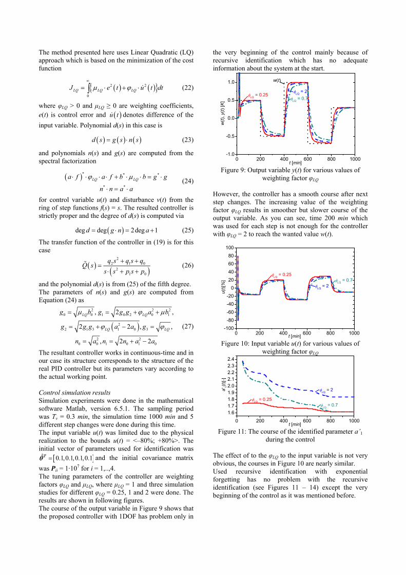
[ ]ˆ 0.1,0.1,0.1,0.1=Τθ and the initial covariance matrix was Pii = 1·107 for i = 1,..,4. The tuning parameters of the controller are weighting factors φLQ and μLQ, where μLQ = 1 and three simulation studies for different φLQ = 0.25, 1 and 2 were done. The results are shown in following figures. The course of the output variable in Figure 9 shows that the proposed controller with 1DOF has problem only in

the very beginning of the control mainly because of recursive identification which has no adequate information about the system at the start.

0 200 400 600 800 1000-1.0

-0.5

0.0

0.5

1.0 w(t)

φLQ = 0.7φLQ = 2

w(t)

, y(t)

[K]

t [min]

φLQ = 0.25

Figure 9: Output variable y(t) for various values of

weighting factor φLQ However, the controller has a smooth course after next step changes. The increasing value of the weighting factor φLQ results in smoother but slower course of the output variable. As you can see, time 200 min which was used for each step is not enough for the controller with φLQ = 2 to reach the wanted value w(t).

0 200 400 600 800 1000-100

-80-60-40-20

020406080

100

u(t)[

%]

t [min]

φLQ = 0.25

φLQ = 2φLQ = 0.7

Figure 10: Input variable u(t) for various values of

weighting factor φLQ

0 200 400 600 800 1000

1.61.71.81.92.02.12.22.32.4

a'1(t)

[-]

t [min]

φLQ = 0.25

φLQ = 2

φLQ = 0.7

Figure 11: The course of the identified parameter a’1

during the control The effect of to the φLQ to the input variable is not very obvious, the courses in Figure 10 are nearly similar. Used recursive identification with exponential forgetting has no problem with the recursive identification (see Figures 11 – 14) except the very beginning of the control as it was mentioned before.

0 200 400 600 800 1000

0.2

0.4

0.6

0.8

1.0

1.2

1.4a'

0(t)[-]

t [min]

φLQ = 0.25φLQ = 2

φLQ = 0.7

Figure 12: The course of the identified parameter a’0

during the control

0 200 400 600 800 1000

-0.034

-0.032

-0.030

-0.028

-0.026

-0.024

b'1(t)

[-]

t [min]

φLQ = 0.25φLQ = 2

φLQ = 0.7

Figure 13: The course of the identified parameter b’1

during the control

0 200 400 600 800 1000-0.05

-0.04

-0.03

-0.02

-0.01

b'0(

t)[-]

t [min]

φLQ = 0.25

φLQ = 2φLQ = 0.7

Figure 14: The course of the identified parameter b’0

during the control CONCLUSION

Paper shows simulation analysis of a continuous stirred tank reactor with ordinary exothermic reaction inside and cooling in the jacket. The mathematical model is constructed by two ordinary differential equations. The simple iteration method and Runge-Kutta’s method were used for numerical solving of steady-state and dynamic analyses. These analyses show mainly nonlinearity of the system and results in the choice of the second order transfer function with relative order one as ELM. Used adaptive control has good control results except for the very beginning of the control because of problems with recursive identification. The output responses after next step changes have smooth course without overshoots. The controller should be tuned via weighting factor φLQ where increasing value of this factor results in smoother but slower response. The used recursive least-squares method with exponential forgetting used for parameter estimation has no problem with the identification after initial “tuning” time. The next step which should follow after this simulation analyses is verification on the real system.

REFERENCES

Åström, K.J. a B. Wittenmark 1989. Adaptive Control. Addison Wesley, Reading, MA.

Bobal, V., Böhm, J., Fessl, J. Machacek, J (2005). Digital Self-tuning Controllers: Algorithms, Implementation and Applications. Advanced Textbooks in Control and Signal Processing. Springer-Verlag London Limited

Fikar, M., Mikles J. 1999. System Identification. STU Bratislava

Gao, R., O’dywer, A., Coyle, E. 2002. A Non-linear PID Controller for CSTR Using Local Model Networks. Proc. of 4th World Congress on Intelligent Control and Automation, Shanghai, P. R. China, 3278-3282

Ingham, J., Dunn, I. J., Heinzle, E., Přenosil, J. E. 2000. Chemical Engineering Dynamics. An Introduction to Modeling and Computer Simulation. Second, Completely Revised Edition, VCH Verlagsgesellshaft, Weinheim.

Kucera, V. 1993. Diophantine equations in control – A survey. Automatica, 29, 1361-1375

Kulhavý, R., Kárný, M. 1984. Tracking of slowly varying parameters by directional forgetting, In: Proc. 9th IFAC World Congress, vol. X, Budapest, 78-83.

Luyben, W. L. 1989. Process Modelling, Simulation and Control for Chemical Engineers. McGraw-Hill, New York.

Middleton, R.H., Goodwin, G.C. 2004 Digital Control and Estimation - A Unified Approach. Prentice Hall, Englewood Cliffs.

Mukhopadhyay, S., Patra, A.G., Rao, G.P. (1992). New class of discrete-time models for continuos-time systeme. International Journal of Control, vol.55, 1161-1187

Stericker, D.L., Sinha, N.K. 1993. Identification of continuous-time systems from samples of input-output data using the δ-operator. Control-Theory and Advanced Technology, vol. 9, 113-125

Vojtěšek, J., Dostál, P., Haber, R. 2004. Simulation and Control of a Continuous Stirred Tank Reactor. In: Proc. of Sixth Portuguese Conference on Automatic Control CONTROLO 2004. Faro. Portugal, p. 315-320.

ACKNOWLEDGMENT

This work was supported by the Ministry of Education of the Czech Rep. under grant No. MSM 7088352101. AUTHOR BIOGRAPHIES

JIRI VOJTESEK was born in Zlin, Czech Republic and studied at the Tomas Bata University in Zlin, where he got his master degree in chemical and process engineering in 2002. He has finished his Ph.D. focused

on Modern control methods for chemical reactors in 2007. His contact is vojtesek@fai.utb.cz.

PETR DOSTAL studied at the Technical University of Pardubice. He obtained his PhD. degree in Technical Cybernetics in 1979 and he became professor in Process Control in 2000. His research interest are

modeling and simulation of continuous-time chemical processes, polynomial methods, optimal, adaptive and robust control. You can contact him on email address dostalp@fai.utb.cz.